Pre-big bang bubbles from the gravitational instability of generic string vacua

Abstract

We formulate the basic postulate of pre-big bang cosmology as one of “asymptotic past triviality”, by which we mean that the initial state is a generic perturbative solution of the tree-level low-energy effective action. Such a past-trivial “string vacuum” is made of an arbitrary ensemble of incoming gravitational and dilatonic waves, and is generically prone to gravitational instability, leading to the possible formation of many black holes hiding singular space-like hypersurfaces. Each such singular space-like hypersurface of gravitational collapse becomes, in the string-frame metric, the usual big-bang $t=0$ hypersurface, i.e. the place of birth of a baby Friedmann universe after a period of dilaton-driven inflation. Specializing to the spherically-symmetric case, we review and reinterpret previous work on the subject, and propose a simple, scale-invariant criterion for collapse/inflation in terms of asymptotic data at past null infinity. Those data should determine whether, when, and where collapse/inflation occurs, and, when it does, fix its characteristics, including anisotropies on the big bang hypersurface whose imprint could have survived till now. Using Bayesian probability concepts, we finally attempt to answer some fine-tuning objections recently moved to the pre-big bang scenario.

I Introduction and general overview

Superstring theory (see [1] for a review) is the only presently known framework in which gravity can be consistently quantized, at least perturbatively. The well-known difficulties met in trying to quantize General Relativity (GR) –or its supersymmetric extensions– are avoided, in string theory, by the presence of a fundamental quantum of length [2] $\ell_{s}\sim(\alpha^{\prime})^{1/2}$. Thus, at distances shorter than $\ell_{s}$, string gravity is expected to be drastically different from –and in particular to be much “softer” than– General Relativity.

However, as was noticed since the early days of string theory [3], a conspicuous difference between string and Einstein gravity persists even at low energies (large distances). Indeed, a striking prediction of string theory is that its “gravitational sector” is richer than that of GR: in particular, all versions of string theory predict the existence of a scalar partner of the spin-two graviton, i.e. of the metric tensor $g_{\mu\nu}$, the so-called dilaton, $\phi$. This field plays a central rôle within string theory [1] since its present vacuum expectation value (VEV) $\phi_{\rm now}$ fixes the string coupling constant $g^{2}=e^{\phi_{\rm now}}$, and, through it, the present values of gauge and gravitational couplings. In particular, it fixes the ratio of $\ell_{s}$ to the Planck length $\ell_{P}\sim G^{1/2}$ by $\ell_{P}\sim g\,\ell_{s}$. The relation is such that gauge and gravitational couplings unify at the string energy scale, i.e. at $E\sim M_{s}\sim gM_{P}\sim(\alpha^{\prime})^{-1/2}\sim 3\times 10^{17}$ GeV. It thus seems that the string way to quantizing gravity forces this new particle/field upon us.

We believe that the dilaton represents an interesting prediction (an opportunity rather than a nuisance) whose possible existence should be taken seriously, and whose observable consequences should be carefully studied. Of course, tests of GR [4] put severe constraints on what the dilaton can do today. The simplest way to recover GR at late times is to assume [5] that $\phi$ gets a mass from supersymmetry-breaking non-perturbative effects. Another possibility might be to use the string-loop modifications of the dilaton couplings for driving $\phi$ toward a special value where it decouples from matter [6]. These alternatives do not rule out the possibility that the dilaton may have had an important rôle in the previous history of the universe. Early cosmology stands out as a particularly interesting arena where to study both the dynamical effects of the dilaton and those associated with the existence of a fundamental length in string theory.

In a series of previous papers [7], [8] a model of early string cosmology, in which the dilaton plays a key dynamical rôle, was introduced and developed: the so-called pre-big bang (PBB) scenario. One of the key ideas of this scenario is to use the kinetic energy of the dilaton to drive a period of inflation of the universe. The motivation is that the presence of a (tree-level coupled) dilaton essentially destroys[9] the usual inflationary mechanism [10]: instead of driving an exponential inflationary expansion, a (nearly) constant vacuum energy drives the string coupling $g=e^{\phi/2}$ towards small values, thereby causing the universe to expand only as a small power of time. If one takes seriously the existence of the dilaton, the PBB idea of a dilaton-driven inflation offers itself as one of the very few natural ways of reconciling string theory and inflation. Actually, the existence of inflationary solution in string cosmology is a consequence of its (T-) duality symmetries [11].

This paper develops further the PBB scenario by presenting a very general class of possible initial states for string cosmology, and by describing their subsequent evolution, via gravitational instability, into a multi-universe comprising (hopefully) sub-universes looking like ours. This picture generalizes, and makes more concrete, recent work [12], [13] about inhomogeneous versions of pre-Big Bang cosmology.

Let us first recall that an inflation driven by the kinetic energy of $\phi$ forces both the coupling and the curvature to grow during inflation [7]. This implies that the initial state must be very perturbative in two respects: i) it must have very small initial curvatures (derivatives) in string units and, ii) it must exhibit a tiny initial coupling $g_{i}=e^{\phi_{i}/2}\ll 1$. As the string coupling $g^{2}$ measures the strength of quantum corrections (i.e. plays the rôle of $\hbar$ in dividing the lagrangian: ${\cal L}=g^{-2}\,{\cal L}^{\prime}$), quantum (string-loop) corrections are initially negligible. Because of i), $\alpha^{\prime}$ corrections can also be neglected. In conclusion, dilaton-driven inflation must start from a regime in which the tree-level low-energy approximation to string theory is extremely accurate, something we may call an asymptotically trivial state.

In the present paper, we consider a very general class of such “past-trivial” states. Actually, perturbative string theory is well-defined only when one considers such classical states as background, or “vacuum”, configurations. For the sake of simplicity the set of string vacua that we consider are already compactified to four dimensions and are truncated to the gravi-dilaton sector (antisymmetric tensor and moduli being set to zero). Within these limitations, the set of all perturbative string vacua coincides with the generic solutions of the tree-level low-energy effective action [14]

$$S_{s}=\frac{1}{\alpha^{\prime}}\int d^{4}x\,\sqrt{G}\,e^{-\phi}[R(G)+G^{\mu\nu}\partial_{\mu}\phi\,\partial_{\nu}\phi]\,,$$ (1)

where we have denoted by $G_{\mu\nu}$ the string-frame ($\sigma$-model) metric. The generic solution is parametrized by 6 functions of three variables. These functions can be thought of classically as describing the two helicity$-2$ modes of gravitational waves, plus the helicity$-0$ mode of dilatonic waves. [Each mode being described by two real functions corresponding, e.g., to the Cauchy data $(\phi,\dot{\phi})$ at some initial time.] The same counting of the degrees of freedom in selecting string vacua can be obtained by considering all the marginal operators (i.e. all conformal-invariance-preserving continuous deformations) of the conformal field theory defining the quantized string in trivial space-time. We therefore envisage, as initial state, the most general past-trivial classical solution of (1), i.e. an arbitrary ensemble of incoming gravitational and dilatonic waves.

Our aim will be to show how such a stochastic bath of classical incoming waves (devoid of any ordinary matter) can evolve into our rich, complex, expanding universe. The basic mechanism we consider for turning such a trivial, inhomogeneous and anisotropic, initial state into a Friedmann-like cosmological universe is gravitational instability (and quantum particle production as far as heating up the universe is concerned [8]). We find that, when the initial waves satisfy a certain (dimensionless) strength criterion, they collapse (when viewed in the Einstein conformal frame) under their own weight. When viewed in the (physically most appropriate) string conformal frame, each gravitational collapse leads to the local birth of a baby inflationary universe blistering off the initial vacuum. Thanks to the peculiar properties of dilaton-driven inflation (i.e. the peculiar properties of collapse with the equation of state $p=\epsilon$), each baby universe is found to contain a large homogeneous patch of expanding space which might constitute the beginning of a local Big Bang. We then expect each of these ballooning patches of space to evolve into a quasi-closed Friedmann universe . This picture is sketched in Fig. 1 and Fig. 2. In order to study in detail this scenario, we focus, in this paper, on the technically simplest case containing nontrivial incoming waves able to exhibit gravitational instability: spherically symmetric dilatonic waves. This simple toy model seems to contain many of the key physical features we wish to study.

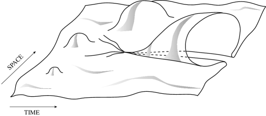
FIG. 1.: Symbolic sketch of the birth of many pre-big bang bubbles from the gravitational instability of a generic string vacuum made of a stochastic bath of classical incoming gravitational and dilatonic waves. Each local Einstein-frame collapse of sufficiently strong waves forms a cosmological-like space-like singularity hidden behind a black hole. The parts of those classical singularities where the string coupling grows inflate, when viewed in the string frame, and generate ballooning patches of space (here schematized as the stretching of one spatial dimension) which are expected to evolve into many separate quasi-closed Friedmann hot universes.

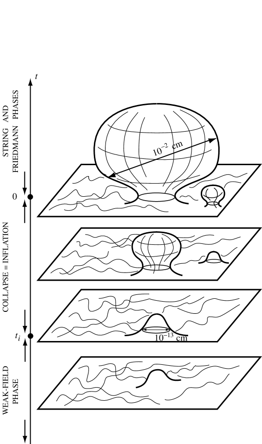
FIG. 2.: A representation of pre-big bang bubbles similar to that of Fig. 1, but in 2+1 dimensions. The different horizontal planes represent different instants in the evolution from the asymptotic trivial past to the Friedmann phase. Two inflationary bubbles characterized by two different initial horizon sizes (both large in string units) are shown to lead to Universes of very different homogeneity scale at the time at which the Hubble radius reaches string-scale values ($\ell_{s}={\cal O}(10^{-32}\,{\rm cm})$).

Before entering the technicalities of this model, let us clarify a few general methodological issues. One of the goals of theoretical cosmology is to “explain” the surprisingly rich and special structure of our universe. However, the concept of “explanation” is necessarily dependent on one’s prejudices and taste. We wish only to show here how, modulo an “exit” assumption [8], one can “explain” the appearance of a hot, expanding homogeneous universe starting from a generic classical inhomogeneous vacuum of string theory. We do not claim that this scenario solves all the cosmological “problems” that one may wish to address (e.g., we leave untouched here the monopole and gravitini problems). We do not try either to “explain” the appearance of our universe as a quantum fluctuation out of “nothing”. We content ourselves by assuming, as is standard in perturbative string theory, the existence of a classical vacuum and showing how gravitational instability can then generate some interesting qualitatively new structures akin to those of our universe. In particular, we find it appealing to “understand” the striking existence of a preferred rest frame in our universe, starting from a stochastic bath of waves propagating with the velocity of light and thereby exhibiting no clear split between space and time. We shall also address in this paper the question of the naturalness of our scenario. Recent papers [18], [19] have insisted on the presence of two large numbers among the parameters defining the PBB scenario. Our answer to this issue (which is, anayway, an issue of taste and not a scientifically well posed problem) is twofold: on the one hand, we point out that the two large numbers in question are classically undefined and therefore irrelevant when discussing the naturalness of a classical vacuum state; on the other hand, we show that the selection effects associated to asking any such “fine-tuning” question can render natural the presence of these very large numbers.

II Asymptotic null data for past-trivial string vacua

Motivated by the pre-Big Bang idea of an initial weak-coupling, low-curvature state we consider the tree-level (order $g^{-2}$) effective action for the gravitational sector of critical superstring theory, taken at lowest order in $\alpha^{\prime}$, Eq. (1). We set to zero the antisymmetric tensor field $B_{\mu\nu}$, and work directly in 4 dimensions (i.e., we assume that the gravitational moduli describing the 6 “internal dimensions” are frozen). Though the physical interpretation of our work is best made in terms of the original string (or $\sigma$-model) metric $G_{\mu\nu}$ appearing in Eq. (1), it will be technically convenient to work with the conformally related Einstein metric

$$g_{\mu\nu}=e^{-(\phi-\phi_{\rm now})}\,G_{\mu\nu}\,,\quad\quad 16\pi G=\alpha^{\prime}\,e^{\phi_{\rm now}}\,.$$ (2)

In the following, we will set $G=1$. In terms of the Einstein metric $g_{\mu\nu}$, the low-energy tree-level string effective action (1) reads

$$S=\frac{1}{16\pi}\int d^{4}x\,\sqrt{g}\,\left[{R}-\frac{1}{2}\partial_{\mu}\phi\,\partial^{\mu}\phi\right]\,.$$ (3)

The corresponding classical field equations are

$$R_{\mu\nu}=\frac{1}{2}\,\partial_{\mu}\phi\,\partial_{\nu}\phi\,,$$ (4)

$$\Box\,\phi\equiv\nabla^{\mu}\,\nabla_{\mu}\,\phi=0\,,$$ (5)

with Eq. (5) actually following from Eq. (4) thanks to the Bianchi identity. As explained in the Introduction, we consider a generic solution of these classical field equations admitting an asymptotically trivial past. Such an asymptotic “incoming” classical state should allow a description in terms of a superposition of ingoing gravitational and dilatonic waves. The work of Bondi, Sachs, Penrose [20] and many others in classical gravitation theory indicates that this incoming state should exhibit a regular past null infinity ${\cal I}^{-}$, and should be parametrizable by some asymptotic null data (i.e. conformally renormalized data on ${\cal I}^{-}$). In plain terms, this means the existence of suitable asymptotically Minkowskian coordinates $(x^{\mu})=(t,x,y,z)$ (which can then be used in the standard way to define polar coordinates $r,\theta,\varphi$ and the advanced time $v\equiv t+r\equiv t+(x^{2}+y^{2}+z^{2})^{1/2}$) such that the following expansions hold when $r\rightarrow\infty$, at fixed $v$, $\theta$ and $\varphi$:

$$\phi(x^{\lambda})=\phi_{0}+\frac{f(v,\theta,\varphi)}{r}+{o}\left(\frac{1}{r}\right)\,,$$ (6)

$$g_{\mu\nu}(x^{\lambda})=\eta_{\mu\nu}+\frac{f_{\mu\nu}(v,\theta,\varphi)}{r}+{o}\left(\frac{1}{r}\right)\,.$$ (7)

The null wave data on ${\cal I}^{-}$ are: the asymptotic dilatonic wave form $f(v,\theta,\varphi)$, and the two polarization components $f_{+}(v,\theta,\varphi)$, $f_{\times}(v,\theta,\varphi)$, of the asymptotic gravitational wave form $f_{\mu\nu}(v,\theta,\varphi)$ . [Introducing a local orthonormal frame ${\bf e}_{(1)}$, ${\bf e}_{(2)}$ on the sphere at infinity one usually defines $f_{+}=\frac{1}{2}(f_{(1)(1)}-f_{(2)(2)})$, $f_{\times}=f_{(1)(2)}$.] The other ${o}(1/r)$ pieces in the metric are gauge dependent, except for the “Bondi mass aspect” $m_{\infty}(v,\theta,\varphi)$ (defined below in a simple case) whose advanced-time derivative is related to the (direction-dependent) incoming energy fluxes:

$$\frac{\partial}{\partial v}\,m_{\infty}(v,\theta,\varphi)=\frac{1}{4}\,(\partial_{v}\,f)^{2}+\frac{1}{4}\,(\partial_{v}\,f_{+})^{2}+\frac{1}{4}\,(\partial_{v}\,f_{\times})^{2}\,+{\rm div.},$$ (8)

where ${\rm div.}$ denotes an angular divergence, $(\sin\theta)^{-1}\,\partial_{\theta}(\sin\theta D^{\theta})+\partial_{\varphi}D^{\varphi}$. Instead of the asymptotic wave forms $f$, $f_{+}$, $f_{\times}$ (which have the dimension of length), one can work with the corresponding “news functions”

$$N(v,\theta,\varphi)\equiv\partial_{v}\,f(v,\theta,\varphi)\ ,\ N_{+}\equiv\partial_{v}\,f_{+}\ ,\ N_{\times}\equiv\partial_{v}\,f_{\times}\,,$$ (9)

which are dimensionless, and whose squares give directly the incoming energy flux appearing on the R.H.S. of Eq. (8).

Before specializing this generic ingoing state, let us note [12], the existence of two important global symmetries of the classical field equations, (4) and (5). They are invariant both under global scale transformations, and under a constant shift of $\phi:ds^{\prime 2}=a^{2}ds^{2}$, $\phi^{\prime}=\phi+b$. [They are also invariant under local coordinate transformations.] In terms of asymptotic data (whose definition requires a specific “flat” normalization of the coordinates at past infinity), the global symmetry transformations read:

$$f(v,\theta,\varphi)\rightarrow f^{\prime}(v^{\prime},\theta,\varphi)=a\,f(v^{\prime}/a,\theta,\varphi)\,,$$ (10)

$$f_{+}(v,\theta,\varphi)\rightarrow f^{\prime}_{+}(v^{\prime},\theta,\varphi)=a\,f_{+}(v^{\prime}/a,\theta,\varphi)\,,$$ (11)

$$f_{\times}(v,\theta,\varphi)\rightarrow f^{\prime}_{\times}(v^{\prime},\theta,\varphi)=a\,f_{\times}(v^{\prime}/a,\theta,\varphi)$$ (12)

with $r\rightarrow r^{\prime}=ar$, $v\rightarrow v^{\prime}=av$, and

$$\phi_{0}\rightarrow\phi^{\prime}_{0}=\phi_{0}+b\,.$$ (13)

Note that the three dimensionless news functions (9) are numerically invariant under the scaling transformations: $N^{\prime}(v^{\prime},\theta,\varphi)=N(v,\theta,\varphi)$, etc. with $v^{\prime}=a\,v$.

As the full time evolution of string vacua depends only on the null data, it is a priori clear that the amplitude of the dimensionless news functions must play a crucial rôle in distinguishing “weak” incoming fields –that finally disperse again as weak outgoing waves– from “strong” incoming fields that undergo a gravitational instability. To study this difficult problem in more detail we turn in the next section to a simpler model with fewer degrees of freedom.

Before doing so, let us comment on the “classicality” of an “in state” defined by some news functions (9). The classical fields (6), (7) deviate less and less from a trivial background $(\phi_{0},\eta_{\mu\nu})$ as $r\rightarrow\infty$ (with fixed $v,\theta$ and $\varphi$). One might then worry that, sufficiently near ${\cal I}^{-}$, quantum fluctuations $\phi^{q}$, $h_{\mu\nu}^{q}$ might start to dominate over the classical deviations $\phi^{c}\equiv\phi(x)-\phi_{0}$, $h_{\mu\nu}^{c}\equiv g_{\mu\nu}-\eta_{\mu\nu}$. To ease this worry let us compute the mean number of quanta in the incoming waves (6), (7). Consider for simplicity the case of an incoming spherically symmetric dilatonic wave $\phi^{c}_{\rm in}=f(v)/r+o(1/r)$. Such an incoming wave has evidently the same mean number of quanta as the corresponding outgoing wave $\phi^{c}_{\rm out}$, with asymptotic behaviour $\phi_{\rm out}^{c}=-f(u)/r+o(1/r)$ , on ${\cal I}^{+}$ ($r\rightarrow\infty$, with $u\equiv t-r,\theta$ and $\varphi$ fixed). As is well known [21], a classical outgoing wave can be viewed, quantum mechanically, as a coherent state in the incoming Fock space defined by the oscillator decomposition of the quantum field $\widehat{\phi}$. Instead of parametrizing $\phi^{c}_{\rm out}$ by the waveform $f(u)$, one can parametrize it by an effective source $J(x^{\lambda})$ such that $\phi^{c}_{\rm out}(x)=\int d^{4}x^{\prime}\,P_{\rm ret}(x-x^{\prime})\,J(x^{\prime})$, where $P_{\rm ret}$ is the (action-normalized) retarded propagator of the field $\phi$. [We use a normalization such that $S=-\frac{1}{2}\,\phi\,P^{-1}\,\phi+J\,\phi$.] The mean number of quanta in the coherent state associated to a classical source $J(x)$ has been computed in [21] for the electromagnetic case, and in [22] for generic massless fields. It reads (with $p\,x\equiv\vec{p}\,\vec{x}-\omega\,t$)

$$\overline{n}=\frac{\pi}{\hbar}\,\int\frac{d^{4}p}{(2\pi)^{4}}\,\delta(p^{2})\,\widehat{J}(-p)\,{\cal R}\,\widehat{J}(p)\,,\quad\quad\widehat{J}(p)\equiv\int d^{4}x\,e^{-ipx}\,J(x)\,,$$ (14)

where ${\cal R}$ denotes the residue of the propagator of the corresponding field, defined such that the field equation $P^{-1}\,\phi=J$ reads $\Box\phi=-{\cal R}\,J$. [In the normalization of the present paper ${\cal R}=16\pi\,G$.] Inserting $J(x)=-(4\,G)^{-1}\,f(t)\,\delta^{(3)}(\vec{x})$ into Eq. (14) yields

$$\overline{n}=\frac{1}{2G\hbar}\,\int_{0}^{\omega}\frac{d\omega}{2\pi}\,\omega\,|\widehat{f}(\omega)|^{2}=\frac{1}{2G\hbar}\,\int_{0}^{\omega}\frac{d\omega}{2\pi}\,\frac{1}{\omega}\,|\widehat{N}(\omega)|^{2}\,,$$ (15)

where $\widehat{N}(\omega)\equiv\int dt\,e^{i\omega t}\,N(t)$ is the one-dimensional Fourier transform of the news function $N(t)=f^{\prime}(t)$. In order of magnitude, if we consider a pulse-like waveform $f(t)$, with characteristic duration $\Delta t\sim\ell_{c}$, and characteristic dimensionless news amplitude $N_{c}\sim f_{c}/\ell_{c}$, the corresponding mean number of quanta is

$$\overline{n}\sim\frac{N_{c}^{2}\,\ell_{c}^{2}}{\ell_{P}^{2}}=\frac{N_{c}^{2}\,\ell_{c}^{2}}{g^{2}\,\ell_{s}^{2}}\,.$$ (16)

In the present paper, we shall consider incoming news functions with amplitude $N_{c}\sim 1$ and scale of variation $\ell_{c}\gg\ell_{s}$. Moreover, in order to ensure a sufficient amount of inflation, the initial value of the string coupling $g^{2}=e^{\phi_{0}}$ has to be $\ll 1$. Therefore, Eq. (16) shows that such incoming states can be viewed as highly classical coherent states, made of an enormous number of elementary $\phi$-quanta: $\overline{n}\gg\!\!>1$. This quantitative fact clearly shows that there is no need to worry about the effect of quantum fluctuations, even near ${\cal I}^{-}$ where $\phi^{c}_{\rm in}\sim f(v)/r\rightarrow 0$. In the case of the negative-curvature Friedmann-dilaton solution this fact has been recently confirmed by an explicit calculation of scalar and tensor quantum fluctuations [23].

III Equations for a spherically symmetric pre-big bang

The simplest nontrivial model which can exhibit the transition between weak, stable data, and gravitationally unstable ones is the spherically-symmetric Einstein-dilaton system. The null wave data for this system comprise only an angle-independent asymptotic dilatonic wave form $f(v)$, corresponding to the dimensionless news function

$$N(v)=\partial_{v}\,f(v)\,.$$ (17)

The spherically symmetric Einstein-dilaton system has been thoroughly studied by many authors with the strongest analytic results appearing in papers by Christodoulou [24]–[26]. A convenient system of coordinates is the double null system, $(u,v)$, such that

$$\phi=\phi(u,v)\,,$$ (18)

$$ds^{2}=-\Omega^{2}(u,v)\,du\,dv+r^{2}(u,v)\,d\omega^{2}\,,$$ (19)

where $d\omega^{2}=d\theta^{2}+\sin^{2}\theta\,d\varphi^{2}$. The field equations are conveniently re-expressed in terms of the three functions $\phi(u,v)$, $r(u,v)$ and $m(u,v)$, where the local mass function $m(u,v)$ is defined by

$$1-\frac{2m}{r}\equiv g^{\mu\nu}\,(\partial_{\mu}r)\,(\partial_{\nu}r)=-\frac{4}{\Omega^{2}}\,\left(\frac{\partial r}{\partial u}\right)_{v}\,\left(\frac{\partial r}{\partial v}\right)_{u}\,.$$ (20)

One gets the following set of evolution equations for $m$, $r$ and $\phi$

$$2\left(\frac{\partial r}{\partial u}\right)_{v}\,\left(\frac{\partial m}{\partial u}\right)_{v}=\left(1-\frac{2m}{r}\right)\,\frac{r^{2}}{4}\,\left(\frac{\partial\phi}{\partial u}\right)_{v}^{2}\,,$$ (21)

$$2\left(\frac{\partial r}{\partial v}\right)_{u}\,\left(\frac{\partial m}{\partial v}\right)_{u}=\left(1-\frac{2m}{r}\right)\,\frac{r^{2}}{4}\,\left(\frac{\partial\phi}{\partial v}\right)^{2}_{u}\,,$$ (22)

$$r\,\frac{\partial^{2}r}{\partial u\partial v}=\frac{2m}{r-2m}\,\left(\frac{\partial r}{\partial u}\right)_{v}\,\left(\frac{\partial r}{\partial v}\right)_{u}\,,$$ (23)

$$r\,\frac{\partial^{2}\phi}{\partial u\partial v}+\left(\frac{\partial r}{\partial u}\right)_{v}\left(\frac{\partial\phi}{\partial v}\right)_{u}+\left(\frac{\partial r}{\partial v}\right)_{u}\left(\frac{\partial\phi}{\partial u}\right)_{v}=0\,.$$ (24)

This double-null evolution system is form-invariant under independent local reparametrizations of $u$ and $v$: $u^{\prime}=U(u)$, $v^{\prime}=V(v)$. To freeze this gauge freedom it is convenient to require that $u=v$ on the central worldline of symmetry $r=0$ (as long as it is a regular part of space-time), and that $v$ and $r$ asymptotically behave like ingoing Bondi coordinates on ${\cal I}^{-}$ (see below).

The quantity

$$\mu(u,v)\equiv\frac{2m(u,v)}{r}$$ (25)

plays a crucial rôle in the problem. Following [26], we shall sometimes call it the “mass ratio”. If $\mu$ stays everywhere below 1, the field configuration will not collapse but will finally disperse itself as outgoing waves at infinity. By contrast, if the mass ratio $\mu$ can reach anywhere the value 1, this signals the formation of an apparent horizon ${\cal A}$. The location of the apparent horizon is indeed defined by the equation

$${\cal A}:\quad\mu(u,v)=1\,.$$ (26)

The above statements are substantiated by some rigorous inequalities [26] stating that:

$$\left(\frac{\partial r}{\partial u}\right)_{v}<0\,,\quad\quad\quad\quad\quad\left(\frac{\partial m}{\partial v}\right)_{u}\geq 0\,,$$ (27)

$$\left(\frac{\partial r}{\partial v}\right)_{u}\,\left(1-\mu\right)\geq 0\,,\quad\quad\left(\frac{\partial m}{\partial u}\right)_{v}\,\left(1-\mu\right)\leq 0\,.$$ (28)

Thus, in weak-field regions ($\mu<1$), $(\partial_{v}r)_{u}>0$, while, as $\mu>1$, $(\partial_{v}r)_{u}<0$, meaning that the outgoing radial null rays (“photons”) emitted by the sphere $r={\rm const.}$ become convergent, instead of having their usual behaviour.

It has been shown long ago that the presence of trapped surfaces implies the existence of some (possibly weak) type of geometric singularity [27], [28]. In the case of the spherically symmetric Einstein-dilaton system, it has been possible to prove [25] that the presence of trapped surfaces (i.e. of an apparent horizon ${\cal A}$ (26), the boundary of the trapped region) implies the existence of a future space-like singular boundary ${\cal B}$ of space-time where the curvature blows up. Both ${\cal A}$ and ${\cal B}$ are “invisible” from future null infinity (${\cal I}^{+}$), being hidden behind an event horizon ${\cal H}$ (a null hypersurface). See Fig. 3.

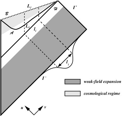
FIG. 3.: Schematic representation of the space-time generated by the collapse of a spherically symmetric pulse of dilatonic waves. An incoming pulse of scalar news $N(v)$, which grows by ${\cal O}(1)$ on an advanced-time scale $\ell_{i}$, collapses to a space-like singularity ${\cal B}$ after having formed an apparent horizon ${\cal A}$ hidden behind the event horizon ${\cal H}$. In the vicinity of ${\cal A}$ and ${\cal H}$, there is an abrupt transition between a weak-field region (dark shading) where the perturbation series (43)–(45) holds, and a strong-field one (light shading) where the cosmological-like expansion (130)–(131) holds.

One of our main purposes in this work is to give the conditions that the incoming dilatonic news function $N(v)$ must satisfy in order to create an apparent horizon, and thereby to lead to some localized gravitational collapse. Before addressing this problem let us complete the description of the toy model by re-expressing it in terms of the ingoing Bondi coordinates $(v,r)$. The metric can now be written in the form

$$ds^{2}=-\left(1-\frac{2m(v,r)}{r}\right)\,e^{2\beta(v,r)}\,dv^{2}+2e^{\beta(v,r)}\,dv\,dr+r^{2}\,d\omega^{2}\,,$$ (29)

and the field equations (21)–(24) become

$$r\,\left(\frac{\partial\beta}{\partial r}\right)_{v}=\frac{r^{2}}{4}\,\left(\frac{\partial\phi}{\partial r}\right)_{v}^{2}\,,$$ (30)

$$2\left(\frac{\partial m}{\partial r}\right)_{v}=\left(1-\frac{2m}{r}\right)\,\frac{r^{2}}{4}\,\left(\frac{\partial\phi}{\partial r}\right)^{2}_{v}\,,$$ (31)

$$2\left(\frac{\partial m}{\partial v}\right)_{r}=e^{-\beta}\,\frac{r^{2}}{2}\,\left[\left(\frac{\partial\phi}{\partial v}\right)_{r}^{2}+e^{\beta}\,\left(1-\frac{2m}{r}\right)\,\left(\frac{\partial\phi}{\partial r}\right)_{v}\,\left(\frac{\partial\phi}{\partial v}\right)_{r}\right]\,,$$ (32)

$$2\left[\frac{\partial^{2}\phi}{\partial v\partial r}+\frac{1}{r}\,\left(\frac{\partial\phi}{\partial v}\right)_{r}\right]+e^{\beta}\left(1-\frac{2m}{r}\right)\,\left(\frac{\partial^{2}\phi}{\partial r^{2}}\right)_{v}+{2e^{\beta}\over r}\,\left(1-\frac{m}{r}\right)\left(\frac{\partial\phi}{\partial r}\right)_{v}=0\,.$$ (33)

Eqs. (30), (31) imply:

$$\partial_{r}\left(e^{\beta(v,r)}\,(r-2m)\right)=e^{\beta(v,r)}\,.$$ (34)

In this coordinate system one can solve for the two functions $\beta(v,r)$ and $\mu(v,r)$ (or $m(v,r)$) by quadratures in terms of the third unknown function $\phi(v,r)$. Indeed, imposing that the coordinate system be asymptotically flat at ${\cal I}^{-}$ (i.e. that $\beta(v,r)\rightarrow 0$ as $r\rightarrow\infty$), one first finds from Eq. (30)

$$\beta(v,r)=-\int_{r}^{+\infty}\frac{dr^{\prime}}{r^{\prime}}\,F(v,r^{\prime})\,,$$ (35)

where

$$F(v,r)\equiv\frac{r^{2}}{4}\,\left(\frac{\partial\phi}{\partial r}\right)_{v}^{2}\,.$$ (36)

Eq. (31) can then be integrated to give

$$\mu(v,r)=\frac{\left[2m_{\infty}(v)-\int_{r}^{+\infty}dr^{\prime}\,F(v,r^{\prime})\,e^{\beta(v,r^{\prime})}\right]}{r\,e^{\beta(v,r)}}\,,$$ (37)

where the “integration constant”

$$m_{\infty}(v)\equiv\lim_{r\rightarrow\infty}m(v,r)$$ (38)

denotes the incoming Bondi mass. By the Bondi energy-flux formula (8), which is also the limiting form of (32) for $r\rightarrow\infty$, $m_{\infty}(v)$ is given in terms of the news function by

$$m_{\infty}(v)=\frac{1}{4}\int_{-\infty}^{v}dv^{\prime}\,N^{2}(v^{\prime})=\,\frac{1}{4}\int_{-\infty}^{v}dv^{\prime}\left(\frac{\partial f(v^{\prime})}{\partial v^{\prime}}\right)^{2}\,,$$ (39)

where we have inserted the asymptotic behaviour of $\phi$ on ${\cal I}^{-}$,

$$\phi(v,r)=\phi_{0}+\frac{f(v)}{r}+{o}\left(\frac{1}{r}\right)\,,$$ (40)

and assumed that $N(v)$ decays sufficiently fast as $v\rightarrow-\infty$ (i.e. near past time-like infinity). From Eqs. (35) and (37) we find the leading asymptotic behaviour of the metric coefficients to be

$$1-\frac{2m(v,r)}{r}=1-\frac{2m_{\infty}(v)}{r}+{o}\left(\frac{1}{r}\right)\,,$$ (41)

$$e^{\beta(v,r)}=1+{\cal O}\left(\frac{1}{r^{2}}\right)\,.$$ (42)

IV Data Strength criterion for gravitational instability

The purpose of this section is to outline the condition that the initial data, i.e. the wave form $f(v)$ or the news function $N(v)\equiv f^{\prime}(v)$, must satisfy in order to undergo, or not undergo, gravitational collapse. A lot of mathematical work has been done on this issue [24]–[26]. In particular, Refs. [24] and [26] gave two different “no collapse” criteria ensuring that the field configuration never collapses and finally disperses out as weak outgoing waves if some functional of the data is small enough. On the other hand, Ref. [25] gave a sufficient “collapse” criterion ensuring that the field configuration will collapse, if some functional of the data is large enough, thereby giving birth to a curvature singularity hidden behind a horizon. The problem with these nice and important mathematical results is threefold: (i) these criteria are sufficient but not necessary, so that they cannot answer our problem of finding (if possible) a sharp criterion distinguishing weak-field from strong-field data; (ii) the various measures of the “strength” of the data given in Refs. [24], [25] and [26] are quite unrelated to each other and do not point clearly toward any sharp “strength criterion”; and (iii) these criteria are not expressed in terms of the asymptotic null data $N(v)$.

Our aim here is not to compete with Refs. [24], [25], [26] on the grounds of mathematical rigour, but to complement these results by a non rigorous study which leads to the iterative computation of a sharp strength criterion, i.e. a functional ${\cal S}[f]$, such that data satisfying ${\cal S}<1$ finally disperse out at infinity, while data satisfying ${\cal S}>1$ are gravitationally unstable and partly collapse to form a singularity. We will then compare our strength functional ${\cal S}$ with the rigorous, but less explicit results of [25]. Note that the emphasis here is not on the question of whether the created singularity is hidden beyond a global event horizon when seen from outside, but rather on the quantitative criterion ensuring that past trivial data give birth to a space-like singularity which we shall later interpret as a budding pre-Big Bang cosmological universe.

A Perturbative analysis in the weak-field region

In view of the discussion of the previous section, the transition between “weak” and “strong” fields is sharply signaled by the appearance of an apparent horizon, i.e. of space-time points where $\mu\equiv 2m/r$ reaches the “critical” value 1. Therefore, starting from the weak-field region near ${\cal I}^{-}$, we can define the strength functional by computing $\mu(u,v)$ as a functional of the null incoming data and by studying if and when it can exceed the critical value. Specifically, we can set up a perturbation analysis of the Einstein-dilaton system in some weak-field domain connected to ${\cal I}^{-}$, and see for what data it suggests that $\mu$ will exceed somewhere the value 1. The expected domain of validity of such a weak-field expansion is sketched in Fig. 3.

The $(u,v)$ system, Eqs. (18) and (19), lends itself easily to a perturbative treatment in the strength of $\phi$. We think here of introducing a formal parameter, say $\lambda$, in the asymptotic data by $f(v)\rightarrow\lambda\,f(v)$ and of constructing the full solution $\phi(u,v)$, $r(u,v)$, $m(u,v)$, as a (formal) power series in $\lambda$ (or by some better iteration method):

$$\overline{\phi}(u,v) \equiv \phi(u,v)-\phi_{0}=\lambda\,\phi_{1}+\lambda^{3}\phi_{3}+\lambda^{5}\phi_{5}+\ldots\,,$$ (43)

$$r(u,v) = \frac{1}{2}\,(v-u)+\lambda^{2}\,r_{2}+\lambda^{4}\,r_{4}+\ldots\,,$$ (44)

$$m(u,v) = \lambda^{2}\,m_{2}+\lambda^{4}\,m_{4}+\ldots\,.$$ (45)

Indeed, knowing $\phi$ to order $\lambda^{2p-1}$ and $r$ to order $\lambda^{2p-2}$ we can use Eq. (21) or (22) to compute by quadrature $m$ to order $\lambda^{2p}$. We can then rewrite Eqs. (23), (24) as

$$\partial_{uv}(r\,\overline{\phi})=\omega\,r\,\overline{\phi}\,,\quad\quad\partial_{uv}\,r=\omega\,r\,,$$ (46)

where

$$\omega\equiv\frac{\mu}{1-\mu}\,\frac{\partial_{u}r\,\partial_{v}r}{r^{2}}\,,$$ (47)

and therefore the right-hand sides of Eqs. (46) are known to (relative) order $\lambda^{2p}$. Solving Eq. (46), then yields $\overline{\phi}$ and $r$ to the next order in $\lambda$ ($\lambda^{2p+1}$ and $\lambda^{2p}$, respectively). To be more explicit, Eqs. (46) are of the form

$$\partial_{uv}\,\psi(u,v)=\sigma(u,v)\,,$$ (48)

where the “source” $\sigma=\omega\psi$ is known at each order in $\lambda$ from the lower-order expression of $\mu$ and $\psi$, and where the “field” $\psi(u,v)$ is restricted to vanish on the central worldline of symmetry $v=u$ (where $r=0$, and $\overline{\phi}$ is regular in the weak-field domain). The generic Eq. (48) can then be solved by introducing the retarded Green function

$$G(u,v;u^{\prime},v^{\prime})=\theta(u-u^{\prime})\,\theta(v-v^{\prime})-\theta(v-u^{\prime})\,\theta(u-v^{\prime})\,,$$ (49)

$$\partial_{uv}\,G(u,v;u^{\prime},v^{\prime})=\delta(u-u^{\prime})\,\delta(v-v^{\prime})\,.$$ (50)

This is the unique Green function in the domain $v\geq u$, $v^{\prime}\geq u^{\prime}$ which vanishes at $v=u$, and whose support in the source point $(u^{\prime},v^{\prime})$ lies in the past of the field point $(u,v)$. The general solution of (48) can then be written as

$$\psi(u,v)=\psi_{\rm in}(u,v)+\int\int_{v^{\prime}\geq u^{\prime}}du^{\prime}\,dv^{\prime}\,G(u,v;u^{\prime},v^{\prime})\,\sigma(u^{\prime},v^{\prime})\,,$$ (51)

where $\psi_{\rm in}(u,v)$ is the free “incoming” field, satisfying $\partial_{uv}\,\psi_{\rm in}=0$ and vanishing when $v=u$, i.e.

$$\psi_{\rm in}(u,v)=g_{\rm in}(v)-g_{\rm in}(u)\,.$$ (52)

The incoming waveform $g_{\rm in}(v)$ is uniquely fixed by the incoming data on ${\cal I}^{-}$. For instance, for $r(u,v)$ asymptotic flatness gives $r_{\rm in}(u,v)=\frac{1}{2}\,(v-u)$ (we recall that in flat space $v=t+r$ and $u=t-r$), while for $\overline{\phi}(u,v)\equiv\phi(u,v)-\phi_{0}$ the asymptotic expansion (40) (in which $f(v)$ was supposed to vanish as $v\rightarrow-\infty$) yields $\overline{\phi}_{\rm in}(u,v)=2(f(v)-f(u))/(v-u)$.

In principle, this perturbative algorithm allows one to compute the mass ratio $\mu(u,v)=2m/r$ to any order in $\lambda$:

$$\mu(u,v)=\lambda^{2}\,\mu_{2}+\lambda^{4}\,\mu_{4}+\ldots\,.$$ (53)

Evidently, the convergence of this series becomes very doubtful when $\mu$ can reach values of order unity, which is precisely when an apparent horizon is formed. One would need some resummation technique to better locate the apparent horizon condition $\mu(v,u)=1$. However, we find interesting to have, in principle, a way of explicitly computing successive approximations to the possible location of an apparent horizon, starting only from the incoming wave data $f(v)$.

B Strength criterion at quadratic order

Let us compute explicitly the lowest-order approximation to (53) (we henceforth set $\lambda=1$ for simplicity). It is obtained by inserting the zeroth-order result $r_{0}(u,v)=\frac{1}{2}\,(v-u)$, and the first-order one for $\phi$

$$\overline{\phi}_{1}(u,v)=\phi_{1}(u,v)-\phi_{0}=\frac{f(v)-f(u)}{r_{0}}=\,\frac{2[f(v)-f(u)]}{v-u}$$ (54)

into Eq. (21) or (22). This yields (with $f^{\prime}(v)\equiv\partial f/\partial v$)

$$\left(\frac{\partial m_{2}}{\partial v}\right)_{u}=r_{0}^{2}\left(\frac{1}{2}\,\frac{\partial\phi_{1}}{\partial v}\right)^{2}=\frac{1}{4}\left[f^{\prime}(v)-\frac{f(v)-f(u)}{v-u}\right]^{2}\,,$$ (55)

$$\left(\frac{\partial m_{2}}{\partial u}\right)_{v}=-r_{0}^{2}\left(\frac{1}{2}\,\frac{\partial\phi_{1}}{\partial u}\right)^{2}=-\frac{1}{4}\left[f^{\prime}(u)-\frac{f(v)-f(u)}{v-u}\right]^{2}\,.$$ (56)

The compatibility of the two equations is easily checked, e.g. by using

$$\partial_{v}(r_{0}^{2}(\partial_{u}\phi_{1})^{2})=r_{0}\,\partial_{u}\phi_{1}\,\partial_{v}\phi_{1}=-\partial_{u}(r_{0}^{2}(\partial_{v}\phi_{1})^{2})\,,$$ (57)

which expresses the “conservation” of the $\phi$-energy tensor in the $(u,v)$ plane. Noting that $m(u,v)$ must vanish (by regularity of $r=0$ in the weak-field domain) at the center $v=u$ one gets, by quadrature, the following explicit result for $m_{2}$:

$$m_{2}(u,v)=\widetilde{m}(u,v)-\frac{1}{8}\ r_{0}\,\overline{\phi}_{1}^{2}\,,$$ (58)

where

$$\widetilde{m}(u,v)\equiv\frac{1}{4}\int_{u}^{v}f^{\prime 2}(x)\,dx\,.$$ (59)

Note that Eq. (58) decomposes $m_{2}(u,v)$ in a “conserved” piece $\widetilde{m}(u,v)=g(v)-g(u)$ (with $\partial_{uv}\widetilde{m}=0$) and a $\phi$-dependent one. This is an integrated form of the local “conservation” law (57) of the $\phi$-energy tensor. Using (58) one gets a very simple result for the quadratic approximation to the mass ratio $\mu=2m/r$, namely

$$\mu_{2}(u,v)=\frac{1}{v-u}\int_{u}^{v}dx\,f^{\prime 2}(x)-\left[\frac{f(v)-f(u)}{v-u}\right]^{2}\,.$$ (60)

Let us introduce a simple notation for the average of any function $g(x)$ over the interval $[u,v]$:

$$\langle g\rangle_{[u,v]}\equiv\langle g(x)\rangle_{x\in[u,v]}\equiv\frac{1}{v-u}\int_{u}^{v}dx\,g(x)\,.$$ (61)

Then the mass ratio, at quadratic order, can be simply written in terms of the scalar news function $N(v)\equiv f^{\prime}(v)$:

$$\mu_{2}(u,v) = \langle N^{2}\rangle_{[u,v]}-(\langle N\rangle_{[u,v]})^{2}\,,$$ (62)

$$= \langle(N(x)-\langle N\rangle_{[u,v]})^{2}\rangle_{x\in[u,v]}\,,$$ (63)

$$\equiv {\rm Var}\,(N(x))_{x\in[u,v]}\,,$$ (64)

where ${\rm Var}\,(g)_{[u,v]}$ denotes the “variance” of the function $g(x)$ over the interval $[u,v]$, i.e. the average squared deviation from the mean.

As indicated above, having obtained $\mu$ to second order, say $\mu_{2}=V(u,v)\equiv{\rm Var}\,(N)_{[u,v]}$, one can then proceed to compute $r$ and $\phi$ to higher orders. Namely, from Eq. (51)

$$2r(u,v)=v-u-G*\left[\frac{V(u,v)}{v-u}\right]+{\cal O}(\lambda^{4})\,,$$ (65)

$$(r\phi)(u,v)=f(v)-f(u)-G*\left[V(u,v)\,\frac{f(v)-f(u)}{(v-u)^{2}}\right]+{\cal O}(\lambda^{5})\,,$$ (66)

where the star denotes a convolution. Then, one can get from these results $m_{4}$, and thereby $\mu_{4}$, by simple quadratures. In the following we shall only use the quadratic approximation to $\mu$, though we are aware that when the initial data are strong enough to become gravitationally unstable, higher order contributions to $\mu$ are probably comparable to $\mu_{2}$.

Finally, at quadratic order, we can define the strength of some initial data simply as the supremum of the variance of the news over arbitrary intervals:

$${\cal S}_{2}=\sup\mu_{2}=\sup_{u,v\atop u\leq v}\,{\rm Var}(N(x))_{x\in[u,v]}\,.$$ (67)

At this order ${\cal S}_{2}<1$ means that $\mu_{2}(u,v)$ stays always below one, i.e. that no trapped region is created, and that the field is expected to disperse, while ${\cal S}_{2}>1$ signals the formation, somewhere, of trapped spheres, and therefore (by the results of [25]) the formation of a singularity. To be more exact we should actually define, in analogy with (67), a quantity ${\cal S}_{2p}=\sup\sum_{k=1}^{p}\mu_{2k}$, at any finite order in the weak field expansion, and state our collapse criterion as the inequality:

$${\cal S}_{2p}>C_{2p}\,,\quad\quad C_{2p}\stackrel{{\scriptstyle p\rightarrow\infty}}{{\rightarrow}}1\,.$$ (68)

In practice, even if we do not expect it to be quantitatively exact, we will use the criterion (68) with $p=1$, taking $C_{2}=1$, hoping that it will be qualitatively correct in capturing the features of the news function which are generically important for producing a gravitational collapse. Let us note that the functional ${\cal S}_{2}$ is (like $N$) dimensionless (and therefore scale invariant) and that it is nonlocal. We note also that it is invariant under a constant shift of $N$, $N(v)\rightarrow N(v)+a$, which corresponds to adding a linear drift in $f:f(v)\rightarrow f(v)+av+b$. Such a shift is (formally) equivalent, in view of Eq. (54), to a constant shift of $\phi_{0}\rightarrow\phi_{0}+2a$.

The non locality of ${\cal S}_{2}$ is physically interesting because it indicates that it is not the instantaneous level of the energy flux $N^{2}(v)$ which really matters, but rather the possibility of having a flux which varies by $\sim$ 100% over some interval of advanced time. This non locality defines also some characteristic scales associated with the collapse (when ${\cal S}_{2}>1$). Indeed, if, by causality, we consider increasing values of $v$, and define ${\cal S}_{2}(v)={\displaystyle\sup_{u,u\leq v}}{\rm Var}(N)_{[u,v]}$, the first value of $v$ for which ${\cal S}_{2}(v)$ exceeds $1$ defines an advanced characteristic time when the collapse occurs, and the corresponding maximizing interval $[u,v]$ defines a characteristic time scale of (in)homogeneity. [Note that $\mu_{2}(u,v)$, Eq. (64), vanishes when $u=v$, and vanishes also generally when $u\rightarrow-\infty$ if $N(u)$ tends to a limit at $-\infty$.]

Let us also mention that our strength functional (67) is superficially similar to the one recently introduced by Christodoulou [26] to characterize sufficiently weak (i.e. non collapsing) data. In the lowest order approximation his criterion measures the strength of the data by ${\cal V}=TV(N(x))$, where $TV$ denotes the total variation (i.e. essentially ${\cal V}=\int_{-\infty}^{+\infty}dv|N^{\prime}(v)|$). Like our variance, this is a measure of the variation of $N(v)$ with, however, a crucial difference. If ${\cal V}$ were a good criterion for measuring the strength of possibly strong data, we would conclude that a news function which oscillates with a very small amplitude for a very long time will be gravitationally unstable, while our criterion indicates that it will not, which seems physically more plausible. We hope that our strength functional (67) will suggest new gravitational stability theorems to mathematicians.

C Comparison with a collapse criterion of Christodoulou

To check the reasonableness of our quadratic strength criterion (67), (68) we have compared it with the rigorous, but only sufficient, collapse criterion of Christodoulou [25], and we have applied it to two simple exact solutions. Ref. [25] gives the following sufficient criterion on the strength of characteristic data considered at some finite retarded time $u$

$$\frac{2\Delta m}{\Delta r}\geq\left[\frac{r_{1}}{r_{2}}\,\log\left(\frac{r_{1}}{2\Delta r}\right)+\frac{6r_{1}}{r_{2}}-1\right]\,,$$ (69)

where $r_{1}\leq r_{2},r_{2}\leq 3r_{1}/2$, are two spheres, $\Delta r=r_{2}-r_{1}$ is the width of the “annular” region between the two spheres, and $\Delta m=m_{2}-m_{1}\equiv m(u,r_{2})-m(u,r_{1})$ is the mass “contained” between the two spheres, i.e. more precisely the energy flux through the outgoing null cone $u={\rm const.}$, between $r_{1}$ and $r_{2}$. Explicitly, from Eq. (31) in $(u,r)$ coordinates, we have

$$2\Delta m=\int_{r_{1}}^{r_{2}}dr\,\frac{r^{2}}{4}\,\left(1-\frac{2m}{r}\right)\,\left(\frac{\partial\phi}{\partial r}\right)^{2}_{u}\,.$$ (70)

We can approximately express this criterion in terms of the incoming null data $N(v)=f^{\prime}(v)$ if we assume that the outgoing cone $u={\rm const.}$ is in the weak-field domain, so that we can replace $\phi$ on the R.H.S. of Eq. (70) by $\phi=r^{-1}[f(u+2r)-f(u)]$. Then the L.H.S. of Eq. (69) becomes (at quadratic order)

$$\frac{2\Delta m}{\Delta r}=\frac{M(u,v_{2})-M(u,v_{1})}{v_{2}-v_{1}}$$ (71)

where

$$M(u,v)\equiv(v-u)\,{\rm Var}(N)_{[u,v]}\equiv\int_{u}^{v}dx\,{\left(N(x)-\langle N\rangle_{[u,v]}\right)}^{2}\,.$$ (72)

Therefore, in this approximation, the criterion of Ref. [25] becomes (with $v_{0}=u$)

$$\exists v_{0},v_{1},v_{2}:\quad\frac{M(v_{0},v_{2})-M(v_{0},v_{1})}{v_{2}-v_{1}}\geq C(v_{0},v_{1},v_{2})\,,$$ (73)

with the constraints $2v_{2}-3v_{1}\leq-v_{0}$, $v_{1}\leq v_{2}$, and the definition

$$C(v_{0},v_{1},v_{2})\equiv\frac{v_{1}-v_{0}}{v_{2}-v_{0}}\,\log\left(\frac{v_{1}-v_{0}}{2(v_{2}-v_{1})}\right)+\frac{6(v_{1}-v_{0})}{v_{2}-v_{0}}-1\,.$$ (74)

If $v_{0}$ is at the boundary of its allowed domain, i.e. if $v_{0}=3v_{1}-2v_{2}$, this criterion is fully compatible with ours since $C(v_{0},v_{1},v_{2})=3$ implying through Eq. (72)

$${\rm Var}(N)_{[v_{0},v_{2}]}\geq 1+\frac{2}{3}\,{\rm Var}(N)_{[v_{0},v_{1}]}\geq 1\,.$$ (75)

In the opposite case ($v_{0}$ large and negative) we think that the criterion (73) is also compatible, for generic news functions, with the general form suggested above, i.e.

$$\exists\,v_{1}^{\prime},v_{2}^{\prime}:\quad{\rm Var}(N)_{[v_{1}^{\prime},v_{2}^{\prime}]}=\langle N^{2}\rangle_{[v_{1}^{\prime},v_{2}^{\prime}]}-\langle N\rangle_{[v_{1}^{\prime},v_{2}^{\prime}]}^{2}\geq C_{2}\,,$$ (76)

with some positive constant $C_{2}$ of order unity. We first note that one should probably impose the physically reasonable condition that $N(v)$ decays sufficiently fast as $v\rightarrow-\infty$ (faster than $|v|^{-1/2}$) to ensure that the integrated incoming energy flux $\int_{-\infty}^{v_{0}}dv\,N^{2}(v)$ is finite. [This constraint freezes the freedom to shift $N(v)$ by a constant.]

When $-v_{0}$ is large, the question remains, however, to know how fast the function $N(v)$ decays when $v_{1}-v$ (for $v_{0}<v<v_{1}$) becomes much larger than $v_{2}-v_{1}$. Let us first consider the physically generic case where $N(v)$ decays in a reasonably fast manner, say faster than a power $|v|^{-\kappa}$ with $\kappa$ of order unity. Then choosing $v_{0}$ in the criterion (73) just large enough to allow one to neglect $N(v_{0})$ with respect to $N(v)$, say $(v_{1}-v_{0})\sim(v_{2}-v_{1})\times 10^{1/\kappa}$, corresponding to $N(v_{0})=0.1\,N(v_{1})$, the L.H.S. of Eq. (73) becomes approximately

$$\frac{2\Delta m}{\Delta r}\simeq\langle N^{2}\rangle_{[v_{1},v_{2}]}\,,$$ (77)

while the function $C$ on the R.H.S., which grows only logarithmically with $v_{0}$, becomes

$$C(v_{0},v_{1},v_{2})\simeq\log\left(\frac{v_{1}-v_{0}}{2(v_{2}-v_{1})}\right)+5\,.$$ (78)

Therefore, a function of the type $N_{\kappa}(v)\sim c\left[(v_{2}-v)/(v_{2}-v_{1})\right]^{-\kappa}$ (when $v\leq v_{1}<v_{2}$) with $c^{2}\,\raise 1.72218pt\hbox{$>$}\kern-6.99997pt\lower 2.6694pt\hbox{$\sim$}\,5+(\log 10)/\kappa$ will fullfil the criterion (73). To see whether this is compatible with our criterion (76) we have studied (analytically and numerically) the variance, over arbitrary intervals $[v_{1}^{\prime},v_{2}^{\prime}]$, of the function $N_{\kappa}(v)$. We found that the inequality (76) is satisfied for a constant $C_{2}^{(\kappa)}$ which is of order unity if $\kappa$ stays of order unity. [For instance, in the extreme case $\kappa=1/2$ corresponding to a logarithmically divergent incoming energy flux, we find $C_{2}^{(1/2)}\sim 0.2$]. We note, however, that if one considers extremely slow decays of $N(v)$, i.e. very small exponents $\kappa\rightarrow 0$ (completed by a faster decay, or an exact vanishing, before some large negative cutoff $v_{c}$ ), the constant $C^{(\kappa)}_{2}$ needed on the R.H.S. of the variance criterion (76) tends to zero. This signals a limitation of applicability of our simple variance criterion based only on the quadratic-order approximation $\mu=\mu_{2}+\mu_{4}+\cdots\simeq\mu_{2}$. Indeed, one can check that, in such an extreme situation $\mu_{2}$ is abnormally cancelled, while $\mu_{4}$ will be of order unity. However, we believe that for generic, non extremely slowly varying news functions, the simple “rule of thumb” (76) is a reasonable approximation to the (unknown) exact collapse criterion. To further check the reasonableness of our criterion (67) we turn our attention to some exact solutions.

D Exact solutions

A first exact, dynamical Einstein-dilaton solution is defined by a news function consisting of the simple step function

$$N(v)=p\,\theta(v)\,.$$ (79)

The corresponding solution has been independently derived by many authors [29]. Here, $p$ is a real parameter and the value $|p|=1$ defines the threshold for gravitational instability: no singularity occurs for $|p|<1$, while $|p|\geq 1$ causes the birth of singularity. The metric for this solution takes the form (note that $\Omega=1$)

$$ds^{2}=-du\,dv+r^{2}\,d\omega^{2}\,,$$ (80)

with the solutions for $\phi$, $r$ and $m$ given as follows:

$$\phi=0\,,\quad\quad r=\frac{1}{2}(v-u)\,,\quad\quad m=0\,,\quad\quad\mbox{ for $v<0$}\,,$$ (81)

while, for $v\geq 0$,

$$\phi(u,v)=-\log\left[\frac{(1-p)\,v-u}{(1+p)\,v-u}\right]\,,$$ (84)

$$r^{2}(u,v)=\frac{1}{4}\,\left[(1-p^{2})\,v^{2}-2v\,u+u^{2}\right]=\frac{1}{4}\,\left[(1-p)\,v-u\right]\,\left[(1+p)\,v-u\right]\,,$$

$$m(u,v)=-\frac{p^{2}\,u\,v}{8r}\,,$$

$$\mu(u,v)=-\frac{p^{2}\,u\,v}{\left[(1-p^{2})\,v^{2}-2v\,u+u^{2}\right]}\,.$$ (85)

Let us note that the perturbation-theory value of $\mu$ for $v>0$, is

$$\mu_{2}{(u,v)}={\rm Var}\,[p\,\theta(x)]_{[u,v]}=-\frac{p^{2}\,u\,v}{(v-u)^{2}}\,\theta(-u)\,.$$ (86)

The maximum value of $\mu_{2}$, reached for $u=-v$, is $p^{2}/4$. This shows that, as expected, the quadratic order criterion (67) is only valid as an order of magnitude, but is quantitatively modified by higher-order corrections. This example, and a related general theorem of Christodoulou [26], suggest that, if the exact criterion were of the type ${\cal S}_{2}=C_{2}$, the constant $C_{2}$ should equal $\frac{1}{4}$. (Note that this value is also compatible with the constant $C_{2}^{(1/2)}\sim 0.2$ appropriate to $|v|^{-1/2}$ decay.)

A second exact solution [30], [18] is a negative-curvature Friedmann-like homogeneous universe. It is defined by the following null data on ${\cal I}^{-}$ (for $v<0$)

$$f(v)=-\frac{\sqrt{3}}{v}\ ,\quad\quad N(v)=\frac{\sqrt{3}}{v^{2}}\,.$$ (87)

Here we view this solution as defined by incoming wave data in a flat Minkowski background. Actually the data are regular only in some advanced cone $v=T+R<0$, and blow up when $v=0$. Here, $T$ and $R=\sqrt{X^{2}+Y^{2}+Z^{2}}$ are usual Minkowski-like coordinates in the asymptotic past. In terms of such coordinates the exact solution reads (when $T^{2}-R^{2}<1$)

$$ds^{2}=\left[1-\frac{1}{(T^{2}-R^{2})^{2}}\right][-dT^{2}+dX^{2}+dY^{2}+dZ^{2}]\,,$$ (88)

$$\phi=-\sqrt{3}\,\log\left(\frac{T^{2}-R^{2}-1}{T^{2}-R^{2}+1}\right)\,.$$ (89)

Note that, for simplicity, we have set here $\phi_{0}=0$, and we have also set the length scale appearing in $f(v)=-\sqrt{3}\,\ell_{0}^{2}/v$ to $\ell_{0}=1$. We shall come back later to the cosmological significance of this solution. Let us only note here that, in terms of the null coordinates

$$u\equiv T-R\ ,\quad\quad v\equiv T+R\,,$$ (90)

the exact mass ratio reads

$$\mu(u,v)=\frac{u\,v\,(v-u)^{2}}{(u^{2}\,v^{2}-1)^{2}}\,,$$ (91)

while, starting from (87), one obtains

$$\mu_{2}{(u,v)}={\rm Var}(N)_{[u,v]}=\frac{(v-u)^{2}}{u^{3}\,v^{3}}\,.$$ (92)

One finds that a strength criterion of the form ${\displaystyle\sup_{u\leq v}}\ \mu_{2}(u,v)=C_{2}$ is first satisfied (as one increases $v$ from $-\infty$) when $v=v_{*2}$, with $u=u_{*2}$, where

$$v_{*2}=-\ell_{0}\left(\frac{4}{27C_{2}}\right)^{1/4}\ ,\quad\quad u_{*2}=3v_{*2}\,.$$ (93)

For $C_{2}$ of order 1, this is in qualitative agreement with the exact result that the apparent horizon is located at

$$u_{\cal A}=\frac{1}{v^{3}}\,,\quad\quad\quad r_{\cal A}=\frac{1}{2|v|^{3}}\,(1-v^{4})^{3/2}\,,$$ (94)

so that the apparent horizon and the singularity are first “seen” at $v_{*\,{\rm exact}}=-\ell_{0}$.

V Transition from the weak-field to the cosmological regime

The following general picture emerges from the previous sections: Let us consider as “in state” a generic classical string vacuum, which can be described as a superposition of incoming wave packets of gravitational and dilatonic fields. This “in state” can be nicely parametrized by three asymptotic ingoing, dimensionless news functions $N(v,\theta,\varphi)$, $N_{+}(v,\theta,\varphi)$, $N_{\times}(v,\theta,\varphi)$. When all the news stay always significantly below 1, this “in state” will evolve into a similar trivial “out state” made of outgoing wave packets. On the other hand, when the news functions reach values of order 1, and more precisely when some global measure of the variation of the news functions, similar to the variance (67), exceeds some critical value of order unity, the “in state” will become gravitationally unstable during its evolution and will give birth to one or several black holes, i.e. one or several singularities hidden behind outgoing null surfaces (event horizons). Seen from the outside of these black holes, the “out” string vacuum will finally look, like the “in” one, as a superposition of outgoing waves. However, the story is very different if we look inside these black holes and shift back to the physically more appropriate string conformal frame. First, we note that the structure of black hole singularities in Einstein’s theory (with matter satisfying $p<\epsilon$) is a matter of debate. The work of Belinsky, Khalatnikov and Lifshitz [31] has suggested the generic appearance of an oscillating space-like singularity. However, the consistency of this picture is unclear as the infinitely many oscillations keep space being as curved (and “turbulent” [32], [33]) as time. Happily, the basic gravitational sector of string theory is generically consistent with a much simpler picture. Indeed, it has been proven long ago by Belinsky and Khalatnikov [34] that adding a massless scalar field (which can be thought of as adding matter with $p=\epsilon$ as equation of state) drastically alters the BKL solution by ultimately quenching the oscillatory behaviour to end up with a much simpler, monotonic approach to a space-like singularity. When described in the string frame, the Einstein-frame collapse towards a space-like singularity will represent (if $\phi$ grows toward the singularity) a super-inflationary expansion of space. The picture is therefore that inside each black hole, the regions near the singularity where $\phi$ grows will blister off the initial trivial vacuum as many separate pre-Big Bangs. These inflating patches are surrounded by non-inflating, or deflating (decreases $\phi$) patches, and therefore globally look approximately closed Friedmann-Lemaître hot universes. This picture is sketched in Fig. 1 and Fig. 2. We expect such quasi-closed universes to recollapse in a finite, though very long, time (which is consistent with the fact that, seen from the outside, the black holes therein contained must evaporate in a finite time). To firm up this picture let us study in detail the appearance of the singularity in the simple toy model of Section III.

A Negative-curvature Friedmann-dilaton solution

We have already seen that in the toy model there is an infinitely extended incoming region where the fields are weak and can be described as perturbations upon the incoming background values $(g_{\mu\nu}^{0}=\eta_{\mu\nu},\phi_{0})$. One expects that the perturbation algorithm described in section IV A becomes unreliable when corrections become of order unity. In particular, one generically expects that the apparent horizon $\mu\equiv\frac{2m}{r}=1$ will roughly divide space-time in two domains: the perturbative incoming weak-field domain where $\mu(u,v)\ll 1$, and a strong-field domain where $\mu(u,v)\gg 1$. [Actually, we shall see below that the precise boundary of the domain of validity of perturbation theory may also depend on other quantities than just $\mu$.] This separation in two domains is represented in Fig. 3.

For guidance let us study in detail this separation in two domains in the case of the $k=-1$ Friedmann-dilaton solution [30], [18]. Let us first write explicitly the solution Eqs. (88) and (89) in $(u,v)$ coordinates

$$ds^{2}=-\Omega^{2}(u,v)\,du\,dv+r^{2}\,d\omega^{2}\,,\quad\quad\phi(u,v)=-\sqrt{3}\,\log\left[\frac{u\,v-1}{u\,v+1}\right]\,,$$ (95)

$$\Omega^{2}(u,v)=\left(1-\frac{1}{u^{2}\,v^{2}}\right)\,,\quad\quad r^{2}(u,v)=\frac{1}{4}\,\left(1-\frac{1}{u^{2}\,v^{2}}\right)\,(u-v)^{2}\,,$$ (96)

$$\mu(u,v)=\frac{u\,v\,(v-u)^{2}}{(u^{2}\,v^{2}-1)^{2}}\,,\quad\quad 1-\frac{2m}{r}=\frac{(u^{3}\,v-1)\,(u\,v^{3}-1)}{(u^{2}\,v^{2}-1)^{2}}\,.$$ (97)

The perturbative algorithm of section IV A gives

$$\phi(u,v) \simeq \frac{2\sqrt{3}}{u\,v}\,\left(1+\frac{1}{3}\frac{1}{u^{2}\,v^{2}}\right)\,,$$ (98)

$$r(u,v) \simeq \frac{1}{2}\,(v-u)\,\left(1-\frac{1}{2}\frac{1}{u^{2}\,v^{2}}\right)\,,$$ (99)

which agree with the expansions of Eqs. (96) and (97). One sees that perturbation theory is numerically valid up to, say, $uv\leq\sqrt{2}$, at which point there is an abrupt transition towards the cosmological singularity located at $uv=1$. Though the transition surface $uv\sim\sqrt{2}$ globally differs from the apparent horizon $\mu(u,v)=1$, we note that our criterion points out to a specific event $(u_{*2},v_{*2})$ on the apparent horizon ${\cal A}$ (the point where ${\cal A}$ is first “seen” from infinity) which lies, roughly, at the intersection of ${\cal A}$ and of the transition surface. This confirms that our criterion is able, at least in order of magnitude, to correctly pinpoint when and where one should shift from the perturbative regime to a different, cosmological-type description. In the case of the solution Eqs. (95)–(97), one sees better the cosmological nature of the strong-field domain by introducing the following coordinates

$$u=-e^{-\eta+\xi}=T-R\,,\quad\quad v=-e^{-\eta-\xi}=T+R\,,$$ (100)

satisfying the useful relations

$$-T=e^{-\eta}\,\cosh\xi\,,\quad\quad\quad R=e^{-\eta}\,\sinh\xi\,,$$ (101)

$$\partial_{u}=e^{\eta-\xi}\,(\partial_{\eta}-\partial_{\xi})\,,\quad\quad\partial_{v}=e^{\eta+\xi}\,(\partial_{\eta}+\partial_{\xi})\,,$$ (102)

$$e^{-2\eta}=u\,v\,,\quad\quad\quad\quad\quad\quad e^{2\xi}=\frac{u}{v}\,.$$ (103)

In terms of the coordinates $(\eta,\xi)$ the solution reads [30], [18]

$$ds^{2}=a^{2}(\eta)\left[-d\eta^{2}+d\xi^{2}+\sinh^{2}\xi\,d\omega^{2}\right]\,,$$ (104)

$$a^{2}(\eta)=4\cosh\eta\,\sinh(-\eta)\,,\quad\quad e^{-\phi}=\left(-\frac{\sinh\eta}{\cosh\eta}\right)^{\sqrt{3}}\,.$$ (105)

We note that the solution is regular in the domain $-\infty<\eta<0$, $0\leq\xi<+\infty$ (which corresponds to the past of the hyperboloid $T^{2}-R^{2}=1$ in Minkowski-like coordinates) and that a space-like singularity is reached at $\eta=0$ (i.e. $uv=T^{2}-R^{2}=1$). Let us also note the expressions

$$r^{2}(\xi,\eta)=a^{2}(\eta)\sinh^{2}\xi=4\cosh\eta\sinh(-\eta)\sinh^{2}\xi\,,$$ (106)

$$1-\frac{2m}{r}=\sinh^{2}\xi\,\left[\coth^{2}\xi-\coth^{2}2\eta\right]\,,$$ (107)

telling us that the apparent horizon is located at $2\eta=-\xi$. Near the singularity, $\eta\rightarrow 0^{-}$, the dilaton blows up logarithmically while the metric coefficients have the following power-law behaviours:

$$\phi\sim-\sqrt{3}\,\log(-\eta)\,,\quad\quad\Omega^{2}(\xi,\eta)\equiv a^{2}(\eta)\sim-4\eta\,,\quad\quad r^{2}(\xi,\eta)\sim-4\eta\sinh^{2}\xi\,.$$ (108)

Before leaving this example we wish to emphasize some features of it which appear to follow from its homogeneity and could be misleading for the general case. The singular boundary terminates, in this case, on ${\cal I}^{-}$, instead of on ${\cal I}^{+}$, as one generically expects. The apparent reason for this is the singularity in the flux at $v=0$ which creates a future boundary on ${\cal I}^{-}$. We believe that, in this case, a better description of physics is obtained by going to new non-Minkowskian coordinates of Milne’s type (see [12]) which automatically incorporate the singularity on ${\cal I}^{-}$. However, if one restricts oneself to more regular initial data, having a finite integrated energy flux (generalized pulse-like data), the singular boundary should never come back to ${\cal I}^{-}$. [At most, it could end at space-like infinity ${i}^{0}$, for non integrable total energy flux].

B Kasner-like behaviour of Einstein-dilaton singularities

Coming back to the generic case of an arbitrary Einstein-dilaton cosmological singularity, previous works [12] have shown that, in a suitable synchronous coordinate system (Gauss coordinates), the asymptotic behaviour of the string frame metric near the singularity reads (in any space-time dimension $D$)

$$ds_{S}^{2}\sim-dt_{S}^{2}+\sum_{a=1}^{D-1}(-t_{S})^{2\alpha_{a}(x)}(E_{i}^{a}(x)\,dx^{i})^{2}\,,$$ (109)

$$\phi(x,t)=\phi(x,0)+\sigma(x)\log(-t_{S})\,,$$ (110)

where $E_{i}^{a}(x)$ is some $(D-1)$-bein and where ($1\leq a\leq D-1$)

$$\sum_{a=1}^{D-1}\alpha_{a}^{2}=1\,,\quad\quad\sigma=\left(\sum_{a=1}^{D-1}\alpha_{a}\right)-1\,.$$ (111)

In the Einstein frame this asymptotic behaviour reads

$$ds_{E}^{2}\sim-dt_{E}^{2}+\sum_{a}(-t_{E})^{2\lambda_{a}(x)}(e_{i}^{a}(x)\,dx^{i})^{2}\,,$$ (112)

$$\phi(x,t)=\phi(x,0)+\gamma(x)\log(-t_{E})\,,$$ (113)

where $e_{i}^{a}(x)$ is proportional to $E_{i}^{a}(x)$ and where

$$\sum_{a=1}^{D-1}\lambda_{a}=1\,,\quad\quad\gamma=\pm\sqrt{2}\ \sqrt{1-\sum_{a=1}^{D-1}\lambda_{a}^{2}}\,.$$ (114)

The “Kasner” exponents, $\alpha_{a}$ in the string frame or $\lambda_{a}$ in the Einstein frame, can vary continuously along the singularity. The string parametrization is the most global one as it shows that $\alpha_{a}$ runs freely over a unit sphere in ${R}^{D-1}$ while the exponent for $e^{\phi}$ is a linear function of the “vector” $\alpha_{a}$. In the Einstein frame, the exponents $\lambda_{a}$ are restricted by the linear equality $\sum_{a}\lambda_{a}=1$ and the quadratic constraint $\sum_{a}\lambda_{a}^{2}\leq 1$. A convenient geometric representation of these constraints, when $D=4$, is to consider (in analogy with Mandelstam’s variables $s,t,u$) that the 3 $\lambda_{a}$’s represent, in some Euclidean plane, the orthogonal distances of a point $\Lambda$ from the three sides of an equilateral triangle (counted positively when $\Lambda$ is inside the triangle). The quadratic constraint then means that $\Lambda$ is restricted to stay inside the circle circumscribing the triangle. The sign ambiguity in Eq. (114) means that the parameter space is in fact a two-sided disk, namely the two faces of a coin circumscribed around the triangle. See Fig. 4.

The link between the two seemingly very different parameter spaces (the string-frame sphere parametrized by the $\alpha$’s and the Einstein-frame two-sided disk parametrized by the $\lambda$’s) is geometrically very simple: one obtains the disk by a stereographic projection of the sphere, from the projection center $(\alpha_{a}^{c})=(1,1,1)$ (outside the sphere) onto the plane dual to this center (i.e. the plane spanning the circle of tangency to the sphere of the straight lines issued from $\alpha^{c}$). Algebraically (in any-space-time dimension $D$)

$$\lambda_{a}=\frac{\alpha_{a}(D-2)-{\sigma}}{D-2-{\sigma}}\,,\quad\quad\gamma=\frac{\sqrt{2\,(D-2)}\,\sigma}{D-2-{\sigma}}\,,$$ (115)

FIG. 4.: Geometric representation of the Einstein-frame Kasner exponents $(\lambda_{1},\lambda_{2},\lambda_{3};\gamma)$ of Einstein-dilaton cosmological singularities. The three $\lambda$’s, such that $\sum_{a}\lambda_{a}=1$ are the orthogonal distances to the three sides of an equilateral triangle. The constraint $\gamma=\pm\sqrt{2}\,\sqrt{1-\sum_{a}\lambda^{2}_{a}}$ restricts the representative $\Lambda$ of $\lambda_{a}$ to stay on a two-sided disk circumscribed around the triangle. The pure-Einstein cases ($\gamma=0$) correspond to the circumscribing circle. In the spherically symmetric case ($\lambda_{2}=\lambda_{3}$), $\Lambda$ runs over a bissectrix of the triangle. The basic parameter $\alpha$ of Eqs. (118) and (128) runs over a full real line (shown folded on the right of the figure ) and is mapped to the bissectrix via horizontal lines.

where $\sigma\equiv(\sum_{a}\alpha_{a})-1$. Note that there is no sign ambiguity in the map $\alpha_{a}\rightarrow\lambda_{a}$. Coming back to the case $D=4$, as $\alpha_{a}$ runs over a unit sphere in ${R}^{3}$, $\lambda_{a}$ covers twice the disk circumbscribed to an equilateral triangle. Each side of the disk is the image, via the stereographic projection, of a polar ($\sigma>0$) or antipolar ($\sigma<0$) “cap” of the sphere. This geometrical picture of the link between the $\alpha$-sphere and the two-sided $\lambda$-disk in represented in Fig. 5. It is useful to keep in mind this geometrical picture because it shows clearly that one can continuously pass from one side of the disk to the other, i.e. the sign of the Einstein-frame “Kasner” exponent of $e^{\phi}\sim(-t_{E})^{\gamma(x)}$ can change as one moves along the singularity. Physically, this means a very striking inhomogeneity near the singularity: the patches where $\gamma(x)>0$ (decreasing $g^{2}=e^{\phi}$) will shrink (in string units) while only the patches where $\gamma(x)<0$ (growing $g^{2}$) can represent pre-Big Bangs. Finally, we note that Belinsky and Khalatnikov [34] have proven that, in the generic case, the Einstein-frame Kasner exponents $(\lambda_{1},\lambda_{2},\lambda_{3})$ must all be positive for the ultimate stable asymptotic approach to the singularity. This corresponds to $\Lambda$ being inside the triangle of Fig. 4, i.e. in the hatched region of Fig. 5. However, this generic restriction does not apply in the special case of our toy model as we explain below.

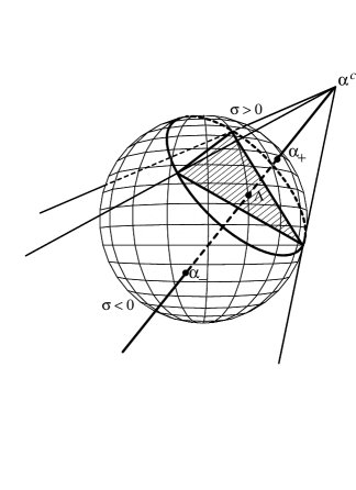
FIG. 5.: Geometrical representation of the link between the two-sided disk of Fig. 4 on which the Einstein-frame Kasner exponents $\lambda_{a}$ live, and the sphere, $\sum_{a}\alpha^{2}_{a}=1$, on which the string-frame Kasner exponents $(\alpha_{1},\alpha_{2},\alpha_{3})$ live. The map $\alpha_{a}\rightarrow\lambda_{a}$ is a stereographic projection, from the center $(\alpha_{a}^{c})=(1,1,1)$. The upper side of the disk comes from the projection of the polar cap $\sigma\equiv(\sum_{a}\alpha_{a})-1>0$ located on the same side as $\alpha^{c}$, while the lower side of the disk comes from projection of the antipolar cap $\sigma<0$. The points $\alpha_{+}$ on the polar cap, and $\alpha_{-}$ on the antipolar cap, are both projected on the same point $\Lambda$ of the disk. The tangents to the sphere issued from $\alpha^{c}$ touch the sphere along the circle limiting the disk (on which $\sigma=0$).

C Behaviour near the singularity in inhomogeneous, spherically symmetric solutions

Let us now restrict ourselves to our toy model and study its cosmological-like behaviour near the singularity. First, we note that spherical symmetry will impose that two of the metric Kasner exponents (those corresponding to the $\theta$ and $\varphi$ directions) must be equal, say $\lambda_{2}=\lambda_{3}$. Geometrically, this means that the Einstein-frame Kasner exponents run only over the intersection of the above two-sided disk with a bissectrix of the triangle. Second, we note that because of the vanishing, in spherical symmetry, of the crucial dreibein connection coefficient $\vec{e}_{1}\cdot(\nabla\times\vec{e}_{1})$, generically responsible for causing the expansion in the (radial) direction $1$ to oscillate as $t\rightarrow 0^{-}$ [31], a negative value of $\lambda_{1}$, corresponding to an expansion in the radial direction, is allowed as ultimate asymptotic behaviour. As a consequence, even the portion of the bissectrix outside the triangle is allowed as asymptotic state. We shall prove directly this fact below by constructing a consistent expansion near the singularity for $\lambda_{1}$ of any sign.

The mass-evolution equations (21), (22), together with Eqs. (27), (28) show that, starting from some regular event at the center, $r=0$, where $m=0$, the mass $m(u,v)$ will grow if we follow a outgoing characteristic (i.e. a null geodesic) $u=$ const. If this characteristic crosses the apparent horizon ${\cal A}$, Eqs. (27), (28) then show that $m(u,v)$ continues to grow within the trapped region ${\cal T}(2m/r>1)$ if one moves along either (future) outgoing or ingoing characteristics. This means that, within ${\cal T}$, $m(u,v)$ grows in all future directions. As the space-like singularity ${\cal B}$ lies in the future of ${\cal T}$, we see that the mass function will necessarily grow toward ${\cal B}$, and therefore, either will tend to a finite limit on ${\cal B}$, or it will tend monotonically to $+\infty$ as $r\rightarrow 0$ with fixed $v$ (or $u$). Motivated by the Kasner-like behaviours Eqs. (112) and (113) we expect the following generic asymptotic behaviour of $m$ on the singularity (here written in $(v,r)$ coordinates)

$$m(v,r)\sim C_{m}(v)\,\left({r\over\ell_{0}}\right)^{-\alpha^{2}(v)}\ \hbox{as}\ r\rightarrow 0\,,v\,\,\hbox{fixed}$$ (116)

with some real $v$-dependent exponent $\alpha^{2}(v)$. [Here $\ell_{0}$ denotes some convenient length scale.] It follows that $\mu=2m/r$ always tends to $+\infty$ on ${\cal B}$ (even when $m$ tends to a finite limit). This suggests that we can consistently compute the structure of the fields near ${\cal B}$ by using an “anti-weak-field” approximation scheme in which $\mu\gg 1$ (instead of the weak-field algorithm of section IV A where we used $\mu\ll 1$). The expected domain of validity of such an “anti-weak-field”, or “cosmological-like”, expansion is sketched in Fig. 3.

To leading order in this large-$\mu$ limit Eq. (31) yields

$$\frac{1}{4}\left(\frac{\partial\phi}{\partial\log r}\right)^{2}_{v}=-\left(\frac{\partial\log m}{\partial\log r}\right)_{v}\,,$$ (117)

from which we obtain the following asymptotic behaviour of $\phi$ on ${\cal B}$

$$\phi(r,v)\sim 2\alpha(v)\log r+C_{\phi}(v)\,.$$ (118)

We see now that the basic Kasner-like-exponent on ${\cal B}$ is half the coefficient of $\log r$ in $\phi(r,v)$ as $r\rightarrow 0$, with fixed $v$. The Kasner-like exponent of $m(v,r)$ is the square of that basic exponent. Moreover, the function $C_{m}(v)$ appearing in the asymptotic behaviour of $m(v,r)$ on the singularity is not independent from the functions $\alpha(v)$ and $C_{\phi}(v)$. Indeed, to leading order Eq. (32) reads

$$\frac{\partial\log m}{\partial v}=-\frac{1}{2}\,\frac{\partial\phi}{\partial\log r}\,\frac{\partial\phi}{\partial v}\,.$$ (119)

This relation is identically satisfied at order $r^{0}\,\log r$, and yields at order $r^{0}$

$$\frac{\partial\log C_{m}}{\partial v}=-\alpha(v)\,\frac{\partial C_{\phi}}{\partial v}\,.$$ (120)

Using now Eq. (30), written as

$$\left(\frac{\partial\beta}{\partial\log r}\right)_{v}=\left(\frac{1}{2}\,\frac{\partial\phi}{\partial\log r}\right)^{2}\,,$$ (121)

we further get the asymptotic behaviour of $\beta(v,r)$

$$\beta(v,r)\sim\alpha^{2}(v)\log r+C_{\beta}(v)\,.$$ (122)

Finally, it is easy to see that the asymptotic behaviour of the metric on ${\cal B}$ in $(v,r)$ coordinates

$$ds^{2}\sim\frac{2C_{m}(v)}{r}\,e^{2C_{\beta}(v)}\,\left({r\over\ell_{0}}\right)^{\alpha^{2}(v)}\,dv^{2}+2e^{C_{\beta}(v)}\,\left({r\over\ell_{0}}\right)^{\alpha^{2}(v)}\,dv\,dr+r^{2}\,d\omega^{2}\,,$$ (123)

is indeed of the expected Kasner form (112) by introducing the cosmological time

$$(-t)\sim r\,\left({r\over\ell_{0}}\right)^{\frac{1}{2}(\alpha^{2}(v)+1)}\,.$$ (124)

The transformed metric reads, to dominant order as $r\rightarrow 0$, i.e. $t\rightarrow 0^{-}$,

$$ds^{2}\sim -dt^{2}+C_{\rho}(v)\,(-t)^{2\lambda_{1}(v)}\,\left(dv+\frac{r\,e^{-C_{\beta}}\,dr}{2C_{m}}\right)^{2}$$ (126)

$$+C_{\omega}(v)\,(-t)^{2\lambda_{2}(v)}\,[d\theta^{2}+\sin^{2}\theta\,d\varphi^{2}]\,,$$

$$\phi\sim\gamma(v)\log(-t)\,,$$ (127)

$$\lambda_{1}(v)=\frac{\alpha^{2}(v)-1}{\alpha^{2}(v)+3}\,,\quad\quad\lambda_{2}(v)=\frac{2}{\alpha^{2}(v)+3}\,,\quad\quad\gamma(v)=\frac{4\alpha(v)}{\alpha^{2}(v)+3}\,.$$ (128)

The basic parameter $\alpha(v)$ runs over the real line $-\infty<\alpha<+\infty$. One easily checks that the relations (114) are satisfied. Some cases having a particular significance are illustrated in Fig. 4: When $\alpha=0$, one gets $(\lambda_{1},\lambda_{2},\lambda_{3})=\left(-\frac{1}{3},\frac{2}{3},\frac{2}{3}\right)$ and $\gamma=0$ which describes a Schwarzschild-like singularity (when viewed with a cosmological eye). When $\alpha=\pm 1$, one gets $(\lambda_{1},\lambda_{2},\lambda_{3})=\left(0,\frac{1}{2},\frac{1}{2}\right)$ and $\gamma=\pm 1$ which is locally similar to the scale-invariant solution [29] also described earlier. When $\alpha=\pm\sqrt{3}$, one gets $(\lambda_{1},\lambda_{2},\lambda_{3})=\left(\frac{1}{3},\frac{1}{3},\frac{1}{3}\right)$ and $\gamma=\pm 2/\sqrt{3}$ which describes an isotropic cosmological singularity of the type of the exact solution [30], [18] we discussed above. As illustrated in Fig. 4, when $\alpha$ runs over ${R}$ its image, defined by Eq. (128), runs twice over the bissectrix of the Mandelstam triangle (intersected with the circumbscribed disk). The only pure-Einstein case ($\gamma=0$) reached at finite $\alpha$ is the Schwarzschild-like case $\alpha=0$. In principle, another pure-Einstein behaviour occurs when $|\alpha|\rightarrow\infty$, leading to $(\lambda_{1},\lambda_{2},\lambda_{3})=(1,0,0)$ i.e. $ds^{2}\sim-dt^{2}+t^{2}\,d\rho^{2}+d\omega^{2}=-d\tau^{2}+d\xi^{2}+d\theta^{2}+\sin^{2}\theta\,d\varphi^{2}$. This would be an Einstein-cylinder-like universe. We believe, however, that $|\alpha(v)|$ will stay bounded $(|\alpha(v)|<\alpha_{M}<+\infty)$ as $v$ runs over ${\cal B}$ and that the only Einstein-like case will be crossed when $\alpha(v)$ changes along ${\cal B}$.

We have confirmed our asymptotic analysis of the structure of the singularity (based on the Ansätze (116), (118) and (122) in two ways. First, we have verified that it is consistent with the partial, but rigorous, results given in Ref. [26]. Namely, in $(u,v)$ coordinates, our Ansätze are compatible with the result that the function $r^{2}(u,v)$ is $C^{1}$ on ${\cal B}$ if we posit that the conformal factor behaves like $\Omega^{2}\sim r^{\alpha^{2}(v)-1}$ (while $m\sim r^{-\alpha^{2}(v)}$). A stronger check of our assumptions is obtained by going beyond the leading order approximation, thus extending some results of [12]. In analogy to section IV A, where we set up a complete perturbation algorithm in the weak-field domain, we have shown that, starting from the leading-order terms Eqs. (116), (118) and (122), containing 3 arbitrary “seed functions”, $\alpha(v)$, $C_{\phi}(v)$, $C_{\beta}(v)$ [from which $C_{m}(v)$ can be determined using Eq. (32)], it is possible to set-up an all-order iterative scheme generating a formal solution of the spherically symmetric Einstein-dilaton system in the strong-field, cosmological-like domain. Note that, $C_{\beta}(v)$ being a pure gauge function (it suffices to introduce $v^{\prime}=\int e^{C_{\beta}(v)}\,dv$ to gauge $C_{\beta}(v)$ away), the formal solution thus generated contains two physically arbitrary functions of $v$, which is indeed the freedom that should be present in a generic solution . Details of this scheme are given in Appendix A. We only mention here the general structure of the expansions so generated near the singularity, i.e. as $r\rightarrow 0$, with fixed $v$: (see Eq. (A35) in the appendix)

$$\phi(v,r)=\phi_{0}(v,r)+\sum_{n,m,l}a_{nml}^{(\phi)}\,r^{n(\alpha^{2}(v)+1)}\,r^{2m}\,P_{l}^{(\phi)}(\log r)\,,$$ (130)

$$\beta(v,r)=\beta_{0}(v,r)+\sum_{n,m,l}a_{nml}^{(\beta)}\,r^{n(\alpha^{2}(v)+1)}\,r^{2m}\,P_{l}^{(\beta)}(\log r)\,,$$

$$m(v,r)=m_{0}(v,r)+\sum_{n,m,l}a_{nml}^{({\rm m})}\,r^{n(\alpha^{2}(v)+1)}\,r^{2m}\,P_{l}^{({\rm m})}(\log r)\,.$$ (131)

Here $n,m,l$ are integers with $l\leq m$, $a_{nml}^{(\psi)}$ and the coefficients of the polynomials $P_{l}^{(\psi)}$ are functions of $v$, and $(\phi_{0},\beta_{0},m_{0})$ are the leading-order terms given by Eqs. (116), (118) and (122). This expansion actually contains two intertwined series: an expansion in powers of $x=r^{1+\alpha^{2}}$ and a more complicated series in $r^{2m}\,(\log r)^{l}$. The second expansion is linked to the $v$-gradients of the seed functions $\alpha(v)$, $C_{\phi}(v)$, $C_{\beta}(v)$, while the first expansion is present even in the simple “homogeneous” case where $\alpha$, $C_{\phi}$ and $C_{\beta}$ do not depend on $v$. The fact, exhibited by Eqs. (130)–(131), that the expansion in the homogeneous case proceeds along powers of $r^{\alpha^{2}+1}$ confirms a recent conjecture by Burko [35].

D Exact homogeneous cosmological solutions

Let us consider in more detail the “homogeneous” case where the seed functions $\alpha$, $C_{\phi}$ and $C_{\beta}$ have no spatial variation along the singularity. As it turns out, it is possible to resum exactly all the terms of the “homogeneous” expansion. Indeed, the analog of the Schwarzschild solution ($t$-independent, spherically symmetric solution) for the Einstein-dilaton system has been worked out analytically long ago by Just [36] (see also [37]), using the special gauge where $g_{00}\,g_{rr}=-1$. Contrary to the case of the Schwarzschild solution, this solution cannot be continuously extended (through a regular horizon) down to a cosmological singularity at $r=0$. However, it is easy to see that the following cosmological-like background (which is related to Just’s original solution by formally extending the radial variable $\overline{r}=l\,x$ “below” the curvature singularity at $\overline{r}=a$) is still a solution of the Einstein-dilaton system:

$$ds^{2} = l^{2}\left[\left(\frac{1-x}{x}\right)^{b}\,dt^{2}-\left(\frac{x}{1-x}\right)^{b}\,dx^{2}+x^{1+b}\,(1-x)^{1-b}\,d\omega^{2}\right]\,,$$ (132)

$$\phi = \pm\sqrt{1-b^{2}}\,\log\left(\frac{1-x}{x}\right)\,.$$ (133)

Here the (formerly radial) variable $x$ varies between $0$ and $1$ and is “time-like”, while the (formerly time) variable $t$ is “space-like”. The cosmological universe evolves from a Big Bang at $x=0$ to a Big Crunch at $x=1$. It has two arbitrary parameters, a scale parameter $l$, and the dimensionless $b$, $-1\leq b\leq 1$. Near the singularity at $x=0$, the link between $b$ and the parametrization used above is

$$\alpha=\mp\sqrt{\frac{1-b}{1+b}}\,,\quad\quad b=\frac{1-\alpha^{2}}{1+\alpha^{2}}\,.$$ (134)

Note that the behaviour near the other singularity at $x=1$ is obtained by changing the sign of $b$ and by changing $\alpha$ into $-1/\alpha$. Some cases of this homogeneous solution are of special significance: $b=1$ is Schwarzschild (with $x=r/2m$), $b=0$ belongs to the class of scale-invariant solutions [29] discussed above and $b=-1/2$ interpolates between a locally isotropic cosmological solution ($\alpha=\mp\sqrt{3}$) at $x=0$ and an anisotropic one ($\alpha=\pm 1/\sqrt{3}$) at $x=1$. Note that, in spite of the homogeneity and isotropy at $x=0$, the latter special solution differs from the (everywhere) homogeneous-isotropic solution described earlier.

E Discussion

Ideally, the two formal expansions we have constructed, the weak-field one Eqs. (43)–(45), and the strong-field one Eqs. (130)–(131), should match at some intermediate hypersurface, like the apparent horizon $2m/r=1$ which looks like a natural borderline between the two near domains. If this matching were analytically doable, it would determine all the (so-far) arbitrary “seed functions” of the strong-field scheme in terms of the unique arbitrary function of the weak-field one, namely the asymptotic waveform $f(v)$ (or, equivalently, the news $N(v)=f^{\prime}(v)$). However, it is clearly too naive to expect to perform this matching perturbatively: neither of the two expansions is expected to be convergent (they are probably only asymptotic). Even if they converge on some domain they probably both break down before reaching a possible overlap region where they might be matched. At this stage, we can only state that, in principle, all the seed functions of the strong-field scheme are some complicated non linear and non local functionals of $N(v)$. It would be particularly interesting to study the functional dependence of the Kasner exponent $\alpha(v)$ on $N(v)$. By causality (i.e. a domain of dependence argument) we know that $\alpha(v)$, at advanced time $v$, depends only on $N(v^{\prime})$ on the interval $v^{\prime}\leq v$. When starting from a generic $N(v)$ “of order unity”, we expect that the resulting $\alpha(v)$ will also be of order unity. A physically very important issue is the sign of $\alpha(v)$, i.e. the sign of $\gamma(v)$. Indeed $\alpha>0$ means a decreasing $\phi$, while $\alpha<0$ means that $\phi$ grows near ${\cal B}$. Let us note that, to lowest-order of weak-field perturbation theory, the value of $\phi(v,r)$ at the (regular) center ($r=0$) is

$$\lim_{r\rightarrow 0}\phi_{1}(v,r)=\lim_{r\rightarrow 0}\left[\phi_{i}+\frac{f(v)-f(v-2r)}{r}\right]=\phi_{i}+2f^{\prime}(v)=\phi_{i}+2N(v)\,.$$ (135)

Here $\phi_{i}$ denotes the background value at past infinity. From this result we expect that, if $N(v)$ is a simple Gaussian-like wave packet, $N(v)=A\exp\left[-(v-v_{i})^{2}/\ell_{i}^{2}\right]$, with a large enough dimensionless amplitude for leading to collapse, i.e. $|A|\gtrsim 1$, the local values of $\phi$ near the collapsing central region will, at first, grow if $A>0$, and decrease if $A<0$. In this simple case, we therefore expect $\alpha(v)$ to have the opposite sign of $A$ near the “central” region of ${\cal B}$, i.e. for $v\lesssim v_{i}$ where the gravitational instability sets in. But, further away on ${\cal B}$, i.e. for $v\gg v_{i}$, the sign of $\alpha(v)$ can change. We also expect that, as $v\rightarrow+\infty$, $\alpha(v)$ will tend to zero, corresponding to a Schwarzschild-like singularity (in the case of well localized incoming $N(v)$ packets). This conjectured link between the sign of $\alpha(v)$ and the sign of $N(v)$ is confirmed by the exact isotropic solution Eq. (95) (with a positive growing $N(v)=\sqrt{3}/v^{2}$, and $\alpha=-\sqrt{3}$), as well as by the scale invariant solution Eq. (84). Some numerical calculations [35] seem to confirm the general picture we propose (in particular the interesting possibility that the sign of $\alpha(v)$ changes several times on ${\cal B}$ as $v$ varies, before reaching a Schwarzschild-like asymptotic regime $|\alpha(v)|\rightarrow 0$ as $v\rightarrow+\infty$). We plan to study in more detail these issues in a future publication.

VI A Bayesian look at pre-Big Bang’s “fine-tuning”

From its inception [38] it was pointed out that a successful pre-Big Bang scenario must rely on a “reservoir” of inflationary $e$-folds during its perturbative phase. This is given by two small numbers, the initial curvature scale in string units, $H_{i}\ell_{s}$, and the initial string coupling constant $g_{i}^{2}=e^{\phi_{i}}\ll\!\!<1$. [In this section, the index $i$ is used for labelling “initial” quantities.] The need of large (or small) numbers has been recently discussed at length [18], [19] and used to criticize the naturalness of the PBB scenario. In particular, it was pointed out [18], [19] that, as soon as one goes beyond the simple spatially-flat, homogeneous cosmology framework, the total duration of the perturbative dilaton-driven phase is finite so that the resolution of the homogeneity/flatness problems requires

$$g_{i}=e^{\phi_{i}/2}<10^{-26}\,,\quad\quad\frac{L_{i}}{\ell_{s}}\gtrsim\frac{M_{s}}{H_{i}}>10^{19}\,.$$ (136)

Here, $L_{i}$ denotes the spatial homogeneity scale of the PBB universe at the beginning of its inflationary phase, and $H_{i}\gtrsim L_{i}^{-1}$ its time-curvature scale (Hubble parameter).

In this Section we shall systematically work with string-frame quantities, even when we refer to results discussed in previous sections in the Einstein frame. For instance, the time-scale $\ell_{i}$, characterizing the rate of variation of the news functions around the advanced time $v_{i}$ and leading to gravitational instability, is now (locally) measured in string units. In any case, we are essentially working with dimensionless ratios which are unit-independent: $(\ell_{i}/\ell_{s})_{S}=(\ell_{i}/\ell_{s})_{E}=g_{i}(\ell_{i}/\ell_{\rm Planck})_{E}$. We wish to emphasize here that, by combining our stochastic-like instability picture with a Bayesian approach to the a posteriori probability of being in a position of asking fine-tuning questions, the issue of the naturalness of the PBB scenario is drastically changed. By “Bayesian approach” we mean taking into account the selection effect that fine-tuning questions presuppose the existence of a scientific civilization. As emphasized long ago by Dicke [39] and Carter [40], civilization-related selection effects can completely change the significance of large numbers or of apparent coincidences. Linde and collaborators explored several aspects of the Dicke-Carter “anthropic principle” within the inflationary paradigm, and emphasized the necessity to weigh a posteriori probabilities by the physical volume of inflationary patches [41]. We shall here follow Vilenkin [42], and his “principle of mediocrity”, according to which the unnormalized a posteriori probability of a random scientific civilization to observe any values of the PBB parameters $g_{i}$, $L_{i}$ and $H_{i}$ is obtained by multiplying the corresponding a priori probability by the number of civilizations (over the whole of space and time) associated with the values $g_{i}$, $L_{i}$ and $H_{i}$: ${\cal N}_{civ}(g_{i},L_{i},H_{i})$.

A A priori and a posteriori probability distributions for $g_{i}$ and $H_{i}$

This approach can be applied to our case if we think of the initial past-trivial string vacuum as made of a more or less stochastic superposition of incoming waves (described by complicated news functions $N(v,\theta,\varphi)$, $N_{+}(v,\theta,\varphi)$, $N_{\times}(v,\theta,\varphi)$ having many bumps, troughs and ramps). This stochastic bath of incoming waves will generate a rough sea of dilatonic and gravitational fields. If the input dimensionless wave forms can reach values of order unity, we expect that the local conditions for gravitational instability will be satisfied at several places in space and time. This will give birth to an ensemble of bubbling baby universes, with a more or less random distribution of initial parameters $g_{i}$ and $H_{i}$, and with initial spatial homogeneity scales $L_{i}\gtrsim H_{i}^{-1}$. Indeed, the analysis of the previous sections has shown (in our toy model) that gravitational instability will set in on a spatio-temporal scale $\sim\ell_{i}$ when a rising wave of news function grows by ${\cal O}(1)$ on an advanced-time scale $\ell_{i}$. From our variance criterion Eq. (67), and the rough validity of weak-field perturbation theory nearly until the sharp transition to a cosmological-type behaviour, the work of the previous sections has shown that the initial, advanced-time scale $\ell_{i}$ is propagated via ingoing characteristics with little deformation down to the strong-field domain (see Fig. 3), where it appears as a spatial homogeneity scale, i.e.

$$L_{i}\sim\ell_{i}\,.$$ (137)

From the leading order result (135) we expect the local value of the Hubble parameter in the corresponding cosmological-like bubble to be

$$H_{i}\sim\sqrt{\dot{\phi}^{2}}\sim|N^{\prime}(v_{i})|\sim\frac{|N(v_{i})|}{\ell_{i}}$$ (138)

where $v_{i}$ denotes the advanced time at which the instability sets in. Combining (137) and (138) we get

$$H_{i}\,L_{i}\sim|N(v_{i})|\gtrsim 1\,.$$ (139)

These rough formulae show how, in principle, given the stochastic properties of the dimensionless news functions, one could deduce the distribution of $H_{i}$ and $L_{i}$, naturally constrained by $H_{i}\,L_{i}\gtrsim 1$. The corresponding distribution of $g_{i}$ is a priori independent from that of $\ell_{i}\sim L_{i}$, being linked to the presence of a slowly-varying (“DC”) component $N_{0}$ in $N(v)$ (by contrast to the local variations of $N(v)$ leading to instability): $N(v)=N_{0}+{\rm fluctuations}$. The DC component $N_{0}$ corresponds to ramps in $f(v)$, $f(v)=N_{0}\,v+f_{0}+{\rm fluctuations}$, i.e. to shifts of $\phi_{i}:\phi_{i}\rightarrow\phi_{i}+2N_{0}$. Finally, we can consider that the initial distribution of the news functions defines an a priori probability distribution for $g_{i}$, and $H_{i}$,

$$dp_{\rm prior}=w_{i}(g_{i},L_{i})\,dg_{i}\,dL_{i}\,,$$ (140)

with $H_{i}$ generically of order $L_{i}^{-1}$ (because $|N(v_{i})|\sim 1$ is the threshold for instability).

An important remark must be made here. The two basic parameters we are talking about, say $g_{i}$ and $L_{i}\sim H_{i}^{-1}$, precisely correspond to the two global symmetries, Eqs. (10)–(12) and Eq. (13), of the classical string vacua: a constant shift in $\phi$, and a global coordinate rescaling. If we consider that the initial state of string theory is classical (rather than quantum), these symmetries mean that no particular values for $\phi_{i}$ or $L_{i}$ are a priori preferred. One might even expect a “flat” distribution compatible with these global symmetries,

$$dp_{\rm prior}^{\rm classical\,flat}\propto\frac{dg_{i}}{g_{i}}\,\frac{dL_{i}}{L_{i}}\propto d\phi_{i}\,d\log L_{i}\,.$$ (141)

Evidently, the problem with such a flat distribution is that it is non-normalizable. Some cut-offs are needed to make sense of such a flat prior distribution but, while there are natural strong coupling/curvature cut-offs (the limits of validity of our approximation), it is not so easy to find natural small-curvature/coupling cut-offs. If we appeal to string theory for providing cut-offs for $g_{i}$ and $L_{i}$, arguably the prior distribution (140) should be determined by the conjectured basic symmetries of string theory, i.e. by $S$ and $T$-duality. $S$-duality suggests that one should work with the complex quantity $z=\frac{\theta}{2\pi}+i\,\frac{4\pi}{g^{2}}$ and require modular invariance in $z=x+iy$. This selects the Poincaré metric $ds^{2}=(dx^{2}+dy^{2})/y^{2}$ as being special, and thereby defines a preferred measure in the fundamental domain (key-hole region) of the $(x,y)$ plane: $d\mu=\sqrt{g}\,dx\,dy=dx\,dy/y^{2}=dx\,|dy^{-1}|$. Integrating out the angular variable $\theta$ over $0\leq\theta<2\pi$ (which is the correct key-hole range when $g^{2}<4\pi$, i.e. $y>1$) we end up with a preferred probability distribution for $g:dp(g)\propto dg^{2}\propto g\,dg$, considered in the weak-coupling region $g\lesssim 1$. A similar argument based on $T$-duality selects as preferred probability distribution for the spatial length scale $L:dp(L)\propto d\widehat{L}^{-2}\,\propto\widehat{L}^{-3}\,d\widehat{L}$ where $\widehat{L}\equiv L/\ell_{s}$ is considered in the weak-$\sigma$-model-coupling region $\widehat{L}\gtrsim 1$. In conclusion, this type of argument would suggest the following normalizable, factorized prior distribution

$$dp_{\rm prior}^{\rm S-T-dual}\propto(g_{i}\,dg_{i})\,\widehat{L}_{i}^{-3}\,d\widehat{L}_{i}\propto g_{i}\,dg_{i}\,\widehat{H}_{i}\,d\widehat{H}_{i}\,,$$ (142)

with $0<g_{i}\lesssim 1$, $0<\widehat{H}_{i}\equiv H_{i}/M_{s}=\widehat{L}_{i}^{-1}\lesssim 1$.

For the sake of generality, we wish to leave open the nature of the prior distribution, and thus consider the general class of prior probability distributions:

$$dp_{\rm prior}\propto g_{i}^{a}\,dg_{i}\,\widehat{H}_{i}^{b}\,d\widehat{H}_{i}\,,$$ (143)

with arbitrary powers $a$ and $b$.

Any given initial distribution, say (143), will generate a corresponding ensemble of PBB inflationary bubbles. We assume, as usual, the existence of a successful “exit” mechanism by which dilaton-driven inflation, with growing $g$ and $H$ finally “exits” into a standard hot Big Bang, i.e. a radiation-dominated Friedmann universe. Current ideas about how this might happen [43] assume that the Hubble parameter reaches values of order of the string mass $M_{s}$, i.e. $\widehat{H}_{s}=H_{s}/M_{s}\sim 1$, before the string coupling constant reaches values of order unity. If the opposite were true ($g\sim 1$ occurring before $\widehat{H}\sim 1$), it is likely that quantum fluctuations would take over before $H$ reaches the string scale, causing inhomogeneities to grow so large that the inflationary process “aborts” before a baby universe is born. In any event, we shall discard this possibility, assuming that the resulting cosmological universe would not evolve into anything able to harbour scientific civilizations.

After $\widehat{H}$ reaches $1$ at $g\ll 1$, the evolving universe is expected to be entering a so-called stringy De Sitter phase, i.e. a phase during which $\dot{\phi}$ and $H$ are constant and given by some fixed-point values of the order of $M_{s}$: $|\dot{\phi}|=x\,M_{s}$, and $|H|=y\,M_{s}$ with $x\sim y\sim 1$. [See [43] for some suggestions on how to implement this mechanism.] Only the ratio between $x$ and $y$ enters our present phenomenological discussion. In keeping with a notation used in previous papers on PBB phenomenology, we introduce the (positive) parameter $\beta$ by

$$|(\ln g)^{\cdot}|=\frac{1}{2}\,|\dot{\phi}|=\beta\,H={\rm const}\,.$$ (144)

One finally assumes that this stringy De Sitter-like phase ends when $g=e^{\phi/2}$ reaches values of order unity, causing the amplified vacuum fluctuations to reach the critical density. After this moment, $g$ should remain fixed at about its present value, either because of a nonperturbative $\phi$-dependent potential, or possibly because of the attractor mechanism of Ref. [6]. The fixing of $g$ marks the end of the stringy modifications to Einstein’s theory, and the beginning of standard Friedmann-like cosmology. As we assume that $g$ is attracted towards a unique fixed point, the resulting Friedmann universe will have no free parameter which could make it different from our universe, except for its initial homogeneity scale $L_{f}$, where the index $f$ refers to the final state of the stringy phase. Therefore, the number of civilizations in the resulting Friedmann universe will be proportional to its total volume, at least for the large enough (in fact, old enough) universes that can harbour life

$${\cal N}_{\rm civ}(g_{i},H_{i})\propto{\cal V}_{f}(g_{i},H_{i})\,\theta[{\cal V}_{f}-{\cal V}_{\min}]\,.$$ (145)

One assumes here, à la Dicke [39], that the time span during which civilizations can occur, being constrained by the lifetime of stars, is fixed. The minimum scale ${\cal V}_{\rm min}$ for a life-harbouring universe is not known precisely, though it corresponds probably to universes whose total lifetime before recollapse is a few billion years. In conclusion, the a posteriori probability for a random scientific civilization to ask fine-tuning questions about the values of $g_{i}$ and $H_{i}$ is

$$dp_{\rm post}\propto{\cal N}_{\rm civ}(g_{i},H_{i})\,dp_{\rm prior}\propto{\cal V}_{f}(g_{i},H_{i})\,\theta({\cal V}_{f}-{\cal V}_{\min})\,dp_{\rm prior}\,.$$ (146)

B Computation of the a posteriori probability distribution in 4 dimensions

The computation of the final volume ${\cal V}_{f}$ can be separated as

$${\cal V}_{f}=L_{f}^{3}=L_{i}^{3}\ \frac{{\cal V}_{1}}{{\cal V}_{i}}\ z_{s}^{3}\,.$$ (147)

Here, the index $i$ refers to the (cosmological) time $t_{i}$ of beginning of dilaton-driven inflation, the index 1 refers to the time $t_{1}$ of transition between dilaton-driven superinflation and a De Sitter-like phase, and $z_{s}=\exp\,(H\,(t_{2}-t_{1}))$ denotes the total expansion during the De Sitter phase. The ending $t_{2}$ of the De Sitter-like phase is assumed to take place whence $g_{2}\equiv g(t_{2})\sim{\cal O}(1)$.

Using the leading power-law behaviour of the cosmological evolution during the dilaton-driven phase, Eq. (109), and imposing that this phase ends when $H_{1}\sim(-t_{1})^{-1}\sim M_{s}$, one gets

$$\frac{{\cal V}_{1}}{{\cal V}_{i}}\simeq\left(\frac{t_{i}}{t_{s}}\right)^{-\Sigma\alpha}\simeq(\widehat{H}_{i})^{\Sigma\alpha}\,,$$ (148)

where $\Sigma\alpha\equiv\alpha_{1}+\alpha_{2}+\alpha_{3}$ is the sum of the string-frame Kasner exponents. The $\alpha$’s are negative (expansion) and are constrained by Eq. (111). In the result (148) we have neglected a factor of order unity linked to the fact that the dilaton-driven inflation is generically anisotropic ($\alpha_{1}\not=\alpha_{2}\not=\alpha_{3}$) and therefore that the various Hubble expansion rates will reach the string scale at slightly different times. We assume here that a nontrivial basin of attraction from anisotropic expansion toward an isotropic stringy De Sitter-like phase exists as it is the case in examples [43].

During the subsequent stringy De Sitter phase, the growth of $g$ is related, according to Eq. (144), to the spatial expansion by $g\propto a^{\beta}$ so that

$$z_{s}=\frac{a_{2}}{a_{1}}=\left(\frac{g_{2}}{g_{1}}\right)^{\frac{1}{\beta}}\sim g_{1}^{-\frac{1}{\beta}}\,,$$ (149)

where we used $g_{2}\sim 1$. On the other hand, $g_{1}=g(t_{1})$ is expressible, through the use of Eq. (110), giving the evolution of $g$ during the dilaton phase, as

$$e^{\phi_{1}-\phi_{i}}=\left(\frac{g_{1}}{g_{i}}\right)^{2}\simeq\left(\frac{t_{1}}{t_{i}}\right)^{\Sigma\alpha-1}\sim\widehat{H}_{i}^{\,\,\Sigma\alpha-1}\,.$$ (150)

Finally, we express, using $L_{i}\sim H_{i}^{-1}$, the volume at the beginning of standard cosmology in the form

$${\cal V}_{f}(g_{i},H_{i})\sim\widehat{H}_{i}^{-A}\,[g_{1}(g_{i},\widehat{H}_{i})]^{-3/\beta}\,\theta(1-g_{1})\,,$$ (151)

with

$$g_{1}(g_{i},\widehat{H}_{i})\sim g_{i}\,\widehat{H}_{i}^{-B}\,,$$ (152)

and where the exponents $A$ and $B$ are positive, and are given in terms of the $\alpha$’s by

$$A=3-\Sigma\alpha\,,\quad\quad B=\frac{1}{2}-\frac{1}{2}\ \Sigma\alpha\,.$$ (153)

If we assume, for illustration, an a priori distribution of values of $g_{i}$ and $\widehat{H}_{i}$ of the form (143), we get for the a posteriori probability distribution of $g_{i}$ and $\widehat{H}_{i}$

$$dp_{\rm post}\propto g_{i}^{a}\,\widehat{H}_{i}^{b-A}\,[g_{i}\,\widehat{H}_{i}^{-B}]^{-3/\beta}\,\theta(1-g_{1}(g_{i},\widehat{H}_{i}))\,\theta({\cal V}_{f}-{\cal V}_{\min})\,dg_{i}\,d\widehat{H}_{i}\,,$$ (154)

which can be written as

$$dp_{\rm post}\propto g_{1}^{\overline{a}}\,\widehat{H}_{i}^{-\overline{A}}\,\theta(1-g_{1})\,\theta({\cal V}_{f}-{\cal V}_{\min})\,dg_{1}\,d\widehat{H}_{i}\,.$$ (155)

In the last form we have expressed the measure $dp_{\rm post}$ in terms of the two independent variables $g_{1}$ and $\widehat{H}_{i}$ (this is convenient because of the constraint $g_{1}<1$ carried by the step function). The exponents $\overline{a}$ and $\overline{A}$ appearing there are

$$\overline{a}\equiv a-\frac{3}{\beta}\,,$$ (156)

$$\overline{A}=A-(a+1)\,B-b=3+\frac{1}{2}\,(a-1)\,(\Sigma\alpha)-\frac{1}{2}\,(a+1)-b\,.$$ (157)

The numerical values of the exponents $\overline{a}$ and $\overline{A}$ play a crucial rôle in determining the a posteriori plausibility of our universe having evolved from the seemingly “unnatural” values (136). Indeed, if $\overline{A}\geq 1$ the posterior probability distribution for $\widehat{H}_{i}$ is peaked, in a non integrable manner, at $\widehat{H}_{i}=0$. Therefore, if $\overline{A}\geq 1$, it is natural to expect (within the present scenario) that the initial homogeneous patch, whose gravitational instability led to our universe, be extremely large compared to the string scale [and that the value of $g_{i}=\widehat{H}_{i}^{B}\,g_{1}$ with $B>0$ and $g_{1}<1$ be correspondingly small]. Most scientific civilizations are bound to evolve in such universes.

Note that the duality-suggested values $a=1$ and $b=1$ of Eq. (143) lead to $\overline{A}=1$ (independently of the $\alpha$’s) for which such an a posteriori explanation works. From this point of view one can argue that, within string theory, it is “natural” to observe very small numbers such as in Eq. (136). The exponent $\overline{a}$ also plays an important rôle. Indeed, if $\overline{a}>-1$, i.e. if

$$\beta>\frac{3}{a+1}\,,$$ (158)

the a posteriori probability distribution for $g_{1}$ is integrable over its entire possible range $(0,1)$. This means that most scientific civilizations are expected to observe values $g_{1}={\cal O}(1)$, corresponding to a small number of $e$-folds during the stringy phase: $z_{s}\sim g_{1}^{-1/\beta}={\cal O}(1)$. This is a phenomenologically interesting case, because it means that various interesting physical phenomena taking place during the dilaton-driven phase (such as the quantum amplification of various fields) might leave observable imprints on cosmologically relevant scales. [A very long string phase would essentially iron out all signals coming from the dilaton phase.] It is interesting to note that, in the string-duality-inspired case (142), the great divide between a short stringy phase $(\overline{a}>-1)$, and a very long one ($\overline{a}\leq-1$, implying that $g_{1}$ is peaked in a non integrable manner at $g_{1}=0$), lies at $\beta=3/2$, which played already a special rôle in previous phenomenological studies [8].

Though the case $\overline{A}\geq 1$, $\overline{a}>-1$ appears as the conceptually most interesting case for the pre-Big Bang scenario, other civilization-related selection effects might also render the case $\overline{A}<1$ viable. In this case, the factors $\widehat{H}_{i}^{-\overline{A}}\,d\,\widehat{H}_{i}$ in Eq. (155) suggests that $\widehat{H}_{i}$ should be of order unity (i.e. $L_{i}\sim H_{i}^{-1}\sim\ell_{s}$). However, in such a case, one must take into account the factor $\theta({\cal V}_{f}-{\cal V}_{\min})$ (which could be neglected in the previous discussion). This factor means that scientific civilizations should a posteriori expect to find themselves in the smallest possible universe compatible with their appearance. This probably means that they should also expect to see inhomogeneities comparable to the Hubble scale, and to have appeared very late in the cosmological evolution, just before the universe recollapses. This seems to conflict with our observations. In conclusion, within this model, and limiting our discussion for simplicity to the class (143) with $a$ and $b$ integers, one finds the favorable situation $\overline{A}\geq 1$ realized (i.e. no a posteriori unnaturalness in observing very small $g_{i}$ and $\widehat{H}_{i}$) when either $a=0$ and $b\leq 2$, or $a=1$ and $b\leq 1$. However, if $a\geq 2$, i.e. if the a priori distribution function of $g_{i}$ vanishes faster than $g_{i}^{2}$ for $g_{i}\rightarrow 0$, the pre-Big Bang scenario has to face a naturalness problem. [This is the case for quantum fluctuations of $g_{i}$, as discussed at the end of the next subsection.]

C Computation of the a posteriori probability distribution in $D$ dimensions

Assuming that the results discussed so far are qualitatively correct in higher dimensions, we have generalized the above considerations to the case in which the initial string vacuum is extended to $d$ spatial dimensions (say $d=9$), and where, through gravitational instability, 3 of these dimensions are expanding and 6 are collapsing down to the string scale. This leads to introducing 4 special times: $t_{i}$ (beginning of dilaton phase), $t_{1}\sim-t_{s}$ (end of the dilaton-driven power-law evolution of space), $t_{2}$ (when the radius of curvature of the collapsing dimensions become ${\cal O}(\ell_{s})$), and $t_{3}$ (when $g_{3}={\cal O}(1)$). In this scenario there are two stringy De Sitter-like phases: a first one during which the 3 “external” dimensions grow exponentially $a\propto\exp\,(H_{1}\,t)$, while the $(d-3)$ “internal” ones shrink exponentially $\overline{a}\propto\exp\,(-\overline{H}_{1}\,t)$ (and while $\dot{\phi}=2\beta_{1}\,H_{1}=2\overline{\beta}_{1}\,\overline{H}_{1}$), and a second phase during which the $(d-3)$ string-scale-curved internal dimensions have frozen while the 3 external ones continue to grow exponentially $a\propto\exp\,(H_{2}\,t)$ (and while $\dot{\phi}=2\beta_{2}\,H_{2}$). This scenario gives a result of the same form as above, namely

$${\cal V}_{f}(g_{i},H_{i})\sim\widehat{H}_{i}^{-A}\,\left[g_{2}(g_{i},\widehat{H}_{i})\right]^{-3/\beta_{2}}\,\theta(1-g_{2})\,,$$ (159)

with

$$g_{2}(g_{i},\widehat{H}_{i})=g_{i}\,\widehat{H}_{i}^{-B}\,,$$ (160)

and where

$$A=d-3\alpha-(d-3)\,\overline{\alpha}+(1-\overline{\alpha})\,\overline{\beta}_{1}\left(\frac{3}{\beta_{1}}-\frac{d-3}{\overline{\beta}_{1}}\right)\,,$$ (161)

$$B=\frac{1}{2}-\frac{3}{2}\,\alpha-\frac{1}{2}\,(d-3)\,\overline{\alpha}+(1-\overline{\alpha})\,\overline{\beta}_{1}\,.$$ (162)

Here one has assumed for simplicity that, during the dilaton phase, the 3 external dimensions grow with the same exponent $\alpha<0$, i.e. proportionally to $(-t)^{\alpha}$, while the $(d-3)$ internal ones decrease with the same exponent $\overline{\alpha}>0$, proportionally to $(-t)^{\overline{\alpha}}$. Then, one can derive the analog of Eq. (155) with $g_{1}$ replaced by $g_{2}$ and with exponents

$$\overline{a}=a-\frac{3}{\beta_{2}}\,\quad\quad\overline{A}=A-(a+1)\,B-b\,.$$ (163)

Once more, $\overline{A}\geq 1$ leads to no fine-tuning and $\overline{a}>-1$ to a short string phase. We shall not attempt a complete phenomenological discussion of the range of values of $a$ and $b$ compatible with $\overline{A}\geq 1$. (This would imply exploring the parameter space of allowed values for the Kasner exponents $\alpha$ and $\overline{\alpha}$.) Let us only note here that the introduction of more spatial dimensions generically helps because $A$ (and $\overline{A}$) now contains the contribution $+d=+9$, say, instead of the previous $+3$. In this case, even distribution functions vanishing faster than $g_{i}^{2}$ (for $g_{i}\rightarrow 0$) can make very small values of $g_{i}$ be a posteriori preferred. The power-law enhancement brought by the volume factor ${\cal V}_{f}$ would be inadequate, however, for compensating an exponential suppression as $g_{i}\rightarrow 0$, say $\propto\exp\,(-c/g_{i}^{2})$. In particular, the a priori distribution of $g_{i}$ and $H_{i}$ cannot be the one expected (from the Lagrangian ${\cal L}\sim e^{-\phi}(\nabla\phi)^{2}\sim(\nabla g^{-1})^{2}$) for quantum fluctuations of $g$ on scales $L_{i}\sim H_{i}^{-1}$ around the trivial ground state. Indeed, this distribution vanishes for small $g_{i}$ and small $\widehat{H}_{i}$ as $\exp\,(-c\,g_{i}^{-2}\,\widehat{H}_{i}^{-2})$ with $c$ of order unity. This confirms the standard idea of the pre-Big Bang scenario, according to which the initial state should be a classical string vacuum, i.e. an arbitrary classical solution of the low-energy field equations.

VII Conclusion

We have proposed a new, concrete picture for the typical initial state of the Universe which can give rise to a cosmology of the so-called pre-big bang type. We conceived this state as a very generic, past-trivial string vacuum, i.e., classically, as the most general solution of the low-energy tree-level string action endowed with a perturbative region in the asymptotic past. Such states can be parametrized (in three spatial dimensions) by three dimensionless “news functions”: a scalar news $N(v,\theta,\varphi)$ and two helicity-2 news $N_{+}(v,\theta,\varphi)$ and $N_{\times}(v,\theta,\varphi)$. By studying the simple spherically symmetric tensor-scalar model we have argued that such a generic “in state” will be gravitationally unstable if (any of) the news functions varie(s) by something of order unity on some scale $\Delta v\sim\ell$. More precisely, in the spherically symmetric model, we found, at lowest order of perturbation theory, that the criterion for gravitational instability is given by the supremum over $v_{1}$ and $v_{2}$ of the variance of the function $N(x)$ over the interval $[v_{1},v_{2}]$, see Eq. (67). When this supremum exceeds a threshold of order unity, the wave packet “sent” between the retarded times $v_{1}$ and $v_{2}$ will become gravitationally unstable when, later, it becomes focussed at the center . We have verified that the infinite region between past infinity and such a center can be described by weak-field perturbation theory. Then, near the center, in a region of spatial extension $L_{i}\sim\Delta v\equiv v_{2}-v_{1}$, one can abruptly shift from a weak-field description to a cosmological one. One can then describe the further evolution of the patch $L_{i}$ by a complementary cosmological-like expansion of the type introduced by Belinsky, Khalatnikov and Lifshitz (BKL) and recently developed, for the PBB scenario, in [12]. We have proven to all orders of iteration (in our toy model) that the presence of the dilaton ensured the consistency of a (non oscillatory) BKL expansion in log-corrected powers of the distance to the future (space-like) singularity. This result confirms the smoothing behaviour of a dilaton-driven superinflationary evolution. In the string frame, gravitationally unstable patches of vacuum, with homogeneity scale $L_{i}$, will expand (if $\dot{\phi}>0$) into homogeneous patches on much larger scales. These blistering patches are surrounded by contracting regions where $\dot{\phi}<0$. Many such dilaton-driven pre-Big Bang inflationary bubbles, looking like closed universes, can blister off a generic past-trivial string vacuum. By taking into account the selection effects linked to the presence of scientific civilizations, we have shown that it can appear a posteriori probable to observe that our universe comes from a very large fluctuation $L_{i}\gg\ell_{s}$, with a very small $g_{i}$. In particular, we pointed out that string-dualities suggest an a priori distribution function for $g_{i}$ and $L_{i}$ which is phenomenologically encouraging in predicting a short, intermediate De Sitter-like stringy phase, and the a posteriori naturalness of observing $L_{i}\gg\ell_{s}$ and $g_{i}\ll 1$.

Our scenario contains new features that might suggest new observable signatures of the pre-Big Bang idea. In particular, we expect the dilaton-driven phase to be generically anisotropic. It will be interesting to study the possible fossils of this anisotropy, especially in the presence of a short string phase. Our work suggests also new types of criteria for the gravitational instability of the Einstein-plus-scalar system. Concentrating on some non cumulative measure of the variation of the news might lead to new theorems of the type of those of Ref. [25], [26].

One of the most interesting well-posed technical problems suggested by our work is the study of the link between the incoming news function and the spatial dependence (along the singularity) of the Kasner exponents. We hope to study this problem in the near future.

A

In this appendix we will establish the structure of the perturbative expansion near the singularity in the spherically symmetric model analysed in the text. We found it more convenient to use the $(v,r)$ coordinate system introduced in Sec. III. The field equations read

$$2\left[\frac{\partial^{2}\phi}{\partial v\partial r}+\frac{1}{r}\,\left(\frac{\partial\phi}{\partial v}\right)\right]+e^{\beta}\left(1-\frac{2m}{r}\right)\,\left(\frac{\partial^{2}\phi}{\partial r^{2}}\right)+{2e^{\beta}\over r}\,\left(1-\frac{m}{r}\right)\left(\frac{\partial\phi}{\partial r}\right)=0\,,$$ (A1)

$$\left(\frac{\partial\beta}{\partial r}\right)=\frac{r}{4}\,\left(\frac{\partial\phi}{\partial r}\right)^{2}\,,\quad\quad 2\left(\frac{\partial m}{\partial r}\right)=\left(1-\frac{2m}{r}\right)\,\frac{r^{2}}{4}\,\left(\frac{\partial\phi}{\partial r}\right)^{2}\,,$$ (A2)

Let us expand the different fields $(\phi,\beta,m)$ around the leading-order solutions (116), (118) and (122)

$$\phi_{0}(v,r) = C_{\phi}(v)+2\alpha(v)\,\log r\,,$$ (A3)

$$\beta_{0}(v,r) = C_{\beta}(v)+\alpha^{2}(v)\,\log r\,,$$ (A4)

$$m_{0}(v,r) = C_{m}(v)\,r^{-\alpha^{2}(v)}\,,$$ (A5)

and define the corrections to it $\overline{\phi},\overline{\beta}$ and $\overline{m}$ by

$$\phi(v,r) = \phi_{0}(v,r)+\overline{\phi}(v,r)\,,$$ (A6)

$$\beta(v,r) = \beta_{0}(v,r)+\overline{\beta}(v,r)\,,$$ (A7)

$$m(v,r) = m_{0}(v,r)\,(1+\overline{m}(v,r))\,.$$ (A8)

Introducing the variable $e^{\lambda}=r$, and denoting differentation with respect to $v$ by a prime, Eqs. (A1)–(A2) take the form:

$$\frac{\partial^{2}\overline{\phi}}{\partial\lambda^{2}} = S_{\phi}(v,\lambda)+L_{\phi}(v,\lambda)+{NL}_{\phi}(v,\lambda)\,,$$ (A9)

$$S_{\phi} = \frac{e^{-C_{\beta}}}{2C_{m}}\,\left[4\alpha^{\prime}\,(1+\lambda)\,e^{2\lambda}+2C_{\phi}^{\prime}\,e^{2\lambda}+2\alpha\,e^{C_{\beta}}\,e^{(\alpha^{2}+1)\,\lambda}\right]\,,$$ (A10)

$$L_{\phi} = \frac{e^{-C_{\beta}}}{C_{m}}\,\left[e^{2\lambda}\,\frac{\partial\overline{\phi}^{\prime}}{\partial\lambda}+e^{2\lambda}\,{\overline{\phi}^{\prime}}+\alpha\,\overline{\beta}\,e^{C_{\beta}}\,e^{(\alpha^{2}+1)\,\lambda}+\frac{e^{C_{\beta}}}{2}\,e^{(\alpha^{2}+1)\,\lambda}\,\left(\frac{\partial^{2}\overline{\phi}}{\partial\lambda^{2}}+\frac{\partial\overline{\phi}}{\partial\lambda}\right)\right]\,,$$ (A11)

$${NL}_{\phi} = \frac{1}{2C_{m}}\,\left[e^{(\alpha^{2}+1)\,\lambda}\,(e^{\overline{\beta}}-1)\,\left(\frac{\partial^{2}\overline{\phi}}{\partial\lambda^{2}}+\frac{\partial\overline{\phi}}{\partial\lambda}\right)-2C_{m}\,(e^{\overline{\beta}}-1)\,(1+\overline{m})\,\frac{\partial^{2}\overline{\phi}}{\partial\lambda^{2}}\,+\right.$$ (A13)

$$\left.2\alpha\,e^{(\alpha^{2}+1)\,\lambda}\,(e^{\overline{\beta}}-1-\overline{\beta})-2C_{m}\,\overline{m}\,\frac{\partial^{2}\overline{\phi}}{\partial\lambda^{2}}\right]\,;$$

$$\left(\frac{\partial\overline{\beta}}{\partial\lambda}\right)-\alpha\,\left(\frac{\partial\overline{\phi}}{\partial\lambda}\right)=S_{\beta}(v,\lambda)+L_{\beta}(v,\lambda)+{NL}_{\phi}(v,\lambda)\,,$$ (A14)

$$S_{\beta}=0=L_{\beta}\,,\quad\quad{NL}_{\phi}=\frac{1}{4}\,\left(\frac{\partial\overline{\phi}}{\partial\lambda}\right)^{2}\,;$$ (A15)

$$\left(\frac{\partial\overline{m}}{\partial\lambda}\right)+\alpha\,\left(\frac{\partial\overline{\phi}}{\partial\lambda}\right)=S_{m}(v,\lambda)+L_{m}(v,\lambda)+{NL}_{m}(v,\lambda)\,,$$ (A16)

$$S_{m}=\frac{\alpha^{2}\,e^{(\alpha^{2}+1)\,\lambda}}{2C_{m}}\,,\quad\quad L_{m}=\frac{\alpha\,e^{(\alpha^{2}+1)\,\lambda}}{2C_{m}}\,\left(\frac{\partial\overline{\phi}}{\partial\lambda}\right)\,,$$ (A17)

$${NL}_{m}=\frac{e^{(\alpha^{2}+1)\,\lambda}}{8C_{m}}\,\left(\frac{\partial\overline{\phi}}{\partial\lambda}\right)^{2}-\frac{1}{4}\,\left(\frac{\partial\overline{\phi}}{\partial\lambda}\right)^{2}-\alpha\,\overline{m}\,\left(\frac{\partial\overline{\phi}}{\partial\lambda}\right)-\frac{\overline{m}}{4}\,\left(\frac{\partial\overline{\phi}}{\partial\lambda}\right)^{2}\,.$$ (A18)

In the R.H.S.’s of Eqs. (A9), (A14) and (A16) we have indicated by $S$ the field-independent terms (“source terms”), by $L$ the terms that are linear in the fields, but subleading with respect to the L.H.S. in the limit $r\rightarrow 0$ ($\lambda\rightarrow-\infty$), while by $NL$ we refer to generic non-linear contributions.

By examining the source terms and the subleading linear terms, we see that they all contain either an explicit factor $e^{(\alpha^{2}+1)\,\lambda}\equiv r^{(\alpha^{2}+1)}$ or a factor $e^{2\lambda}\equiv r^{2}$. To keep track of the presence of these factors (which tend to zero at the singularity) let us introduce two formal bookkeeping parameters: $\sigma_{1}$ associated with each occurrence of $e^{(\alpha^{2}+1)\,\lambda}$ in $S$ and $L$ and, likewise, $\sigma_{2}$ associated with $e^{2\lambda}$. In the end we shall set $\sigma_{1}=\sigma_{2}=1$, but the introduction of these parameters will be useful to delineate the structure of the expansion of the fields near $r=0$.

Introducing the notation $\psi=(\overline{\phi},\overline{\beta},\overline{m})$, considered as a column matrix, and denoting $D_{\lambda}$ the following derivative operator with respect to $\lambda$,

$$D_{\lambda}=\left(\begin{array}[]{ccc}\partial_{\lambda}^{2}&0&0\\ -\alpha(v)\partial_{\lambda}&\partial_{\lambda}&0\\ +\alpha(v)\partial_{\lambda}&0&\partial_{\lambda}\end{array}\right)\,,$$ (A19)

we can rewrite Eqs. (A9), (A14) and (A16) in the compact matrix form:

$$D_{\lambda}\psi=\sigma_{1}\,S_{\psi}^{(1)}+\sigma_{2}\,S_{\psi}^{(2)}+\sigma_{1}\,L_{\psi}^{(1)}+\sigma_{2}\,L_{\psi}^{(2)}+{NL}_{\psi}\,.$$ (A20)

The nonlinear terms in (A20) depend linearly on $\sigma_{1}$ and $\sigma_{2}$: ${NL}_{\psi}(\psi,\partial_{\lambda}\psi,\partial_{\lambda}^{2}\psi,\sigma_{1},\sigma_{2})={NL}_{\psi}^{(0)}+\sigma_{1}\,{NL}_{\psi}^{(1)}+\sigma_{2}\,{NL}_{\psi}^{(2)}$. The differential matrix system (A20) can be rewritten as an integro-differential system by introducing the “retarded” Green function $G(\lambda,\lambda^{\prime})$, i.e. the unique inverse of $D_{\lambda}$ which vanishes when $\lambda^{\prime}>\lambda$

$$\psi=G*\left(\sigma_{1}\,S_{\psi}^{(1)}+\sigma_{2}\,S_{\psi}^{(2)}+\sigma_{1}\,L_{\psi}^{(1)}+\sigma_{2}\,L_{\psi}^{(2)}+{NL}_{\psi}\right)\,,$$ (A21)

where we indicate by $*$ the operation of integrating over $\lambda^{\prime}$. This choice of boundary conditions is imposed by consistency: We defined the background solution (A3)–(A5) as giving the asymptotic behaviour of $(\phi,\beta,m)$ when $r\rightarrow 0$, i.e. $\lambda\rightarrow-\infty$ . We must therefore require that the deviation field $\psi(\lambda)$ vanish when $\lambda\rightarrow-\infty$.

The system (A21) can be formally solved by successive iterations, leading to a solution $\psi$ in the form of a double power series in the bookkeeping parameters $\sigma_{1}$ and $\sigma_{2}$:

$$\psi=\sum_{n,m\geq 1}\sigma_{1}^{n}\,\sigma_{2}^{m}\,\psi_{nm}\,.$$ (A22)

For instance, the first order (in $\sigma_{1}$ and $\sigma_{2}$) corrections $\psi_{1}=\sigma_{1}\,\psi_{10}+\sigma_{2}\,\psi_{01}$, i.e. the next-to-leading-order terms in Eqs. (A6)–(A8), are obtained by neglecting the $L$ and $NL$ terms. They satisfy the equations

$$\frac{\partial^{2}\phi_{1}}{\partial\lambda^{2}}=S_{\phi}(v,\lambda)\,,$$ (A23)

$$\left(\frac{\partial\beta_{1}}{\partial\lambda}\right)-\alpha(v)\left(\frac{\partial\phi_{1}}{\partial\lambda}\right)=S_{\beta}(v,\lambda)\,,$$ (A24)

$$\left(\frac{\partial m_{1}}{\partial\lambda}\right)+\alpha(v)\left(\frac{\partial\phi_{1}}{\partial\lambda}\right)=S_{m}(v,\lambda)\,.$$ (A25)

The unique solution of this system which vanishes when $\lambda\rightarrow-\infty$ reads

$$\phi_{1}(v,\lambda) = \int^{\lambda}_{-\infty}d\lambda^{\prime}\,\int^{\lambda^{\prime}}_{-\infty}d\lambda^{\prime\prime}\,S_{\phi}(v,\lambda^{\prime\prime})=\int^{\lambda}_{-\infty}d\lambda^{\prime}\,(\lambda-\lambda^{\prime})\,S_{\phi}(v,\lambda^{\prime})\,,$$ (A26)

$$\beta_{1}(v,\lambda) = \alpha(v)\,\phi_{1}(v,\lambda)+\int^{\lambda}_{-\infty}d\lambda^{\prime}\,S_{\beta}(v,\lambda^{\prime})\,,$$ (A27)

$$m_{1}(v,\lambda) = -\alpha(v)\,\phi_{1}(v,\lambda)+\int^{\lambda}_{-\infty}d\lambda^{\prime}\,S_{m}(v,\lambda^{\prime})\,.$$ (A28)

The form of this solution defines the action $G*S\equiv\int d\lambda^{\prime}\,G(\lambda,\lambda^{\prime})\,S(\lambda^{\prime})$ of the retarded matrix Green function $G(\lambda,\lambda^{\prime})$ on any source term $S(\lambda^{\prime})=(S_{\phi}(\lambda^{\prime}),S_{\beta}(\lambda^{\prime}),S_{m}(\lambda^{\prime}))$. As a check on the consistency of the iteration method, note that, if one had not imposed any boundary conditions, the generic solution $\psi_{1}$ would have contained an arbitrary homogeneous solution $\psi_{\rm hom}$ (“zero mode”). However, it is easy to check that the addition of such a generic $\psi_{\rm hom}$ would be absorbable in suitable redefinitions of the “seed” functions $\alpha(v),C_{\phi}(v)$, $C_{\beta}(v)$, $C_{m}(v)$ entering the background solution Eqs. (A3)–(A5). Finally, the explicit form of the next-to-leading order solution (with $\sigma_{1}=\sigma_{2}=1$) is

$$\phi_{1}(v,\lambda) = \frac{\alpha}{(\alpha^{2}+1)^{2}\,C_{m}}\,{e^{(\alpha^{2}+1)\,\lambda}}\,+\frac{C_{\phi}^{\prime}\,e^{-C_{\beta}}}{4C_{m}}\,e^{2\lambda}+\frac{\alpha^{\prime}\,e^{-C_{\beta}}}{2C_{m}}\,\lambda\,e^{2\lambda}\,,$$ (A29)

$$\vrule width=0.0pt,height=18.0pt,depth=15.0pt\beta_{1}(v,\lambda) = \alpha\,\phi_{1}(v,\lambda)\,,$$ (A30)

$$m_{1}(v,\lambda) = -\alpha\,\phi_{1}(v,\lambda)+\frac{\alpha^{2}}{2(\alpha^{2}+1)C_{m}}\,{e^{(\alpha^{2}+1)\,\lambda}}\,.$$ (A31)

Note that the coefficients of the terms proportional to $e^{2\lambda}$ and $\lambda\,e^{2\lambda}$ contain derivatives with respect to $v$, hence they determine the inhomogeneous expansion near the singularity, while the terms proportional to $e^{(\alpha^{2}+1)\,\lambda}$ are present also in the purely homogeneous case.

Inserting the double power series expansion (A22) into (A20) or (A21) yields, for each contribution $\psi_{nm}$,

$$D_{\lambda}\psi_{nm}=s_{nm}\,,\quad\quad\psi_{nm}=G*s_{nm}\,,$$ (A32)

where the R.H.S. $s_{nm}$ plays, at each order, the rôle of an effective source term which is (in principle) known, being some algebraico-differential expression in the lower-order terms $\psi_{n^{\prime}m^{\prime}}$, with $n^{\prime}+m^{\prime}<n+m$. Let us make the inductive assumption that $s_{nm}$ is a sum of terms of the form

$$s_{nml}=e^{n\,(\alpha^{2}+1)\,\lambda}\,e^{2m\,\lambda}\,Q_{l}(\lambda)\,,$$ (A33)

with $l\leq m$, where $Q_{l}(\lambda)$ is a polynomial in $\lambda$ of order $l$. [Here, $n,m,l$ are all integers]. It is straightforward to check, from the explicit action (A26)–(A28) of the Green function on source terms, that the solution $\psi_{nml}$ corresponding to any term $s_{nml}$, Eq. (A33), in the R.H.S. of Eq. (A32) is again of the form

$$\psi_{nml}=G*s_{nml}=e^{n\,(\alpha^{2}+1)\,\lambda}\,e^{2m\,\lambda}\,\widetilde{Q}_{l}(\lambda)\,,$$ (A34)

where $\widetilde{Q}_{l}(\lambda)$ is another polynomial in $\lambda$, of the same order $l$. Examining the explicit form of the $L$ and $NL$ terms on the R.H.S. of Eqs. (A9), (A14) and (A16), one can then prove that the induction hypothesis consistently propagates at the next order in $n+m$ (still with the constraint $l\leq m$).

In conclusion, coming back to the variable $r$, we find that the inhomogeneous expansion near the singularity contains two intertwined series: an expansion in powers of $r^{(\alpha^{2}+1)}$ and one in powers of $r^{2}$ mixed with powers of $\log r$. The solution to all orders will be of the form:

$$\psi=\sum_{n,\,m,\,l\leq m}a_{nml}\,r^{n(\alpha^{2}+1)}\,r^{2m}\,P_{l}(\log r)\,,$$ (A35)

where $a_{nml}$, and the coefficients of the polynomial $P_{l}$, are functions of $v$ that in principle can be iteratively evaluated. As shown in Sec. V D, the full subseries $\sum_{n}a_{n00}\,r^{n\,(\alpha^{2}+1)}$ can be exactly summed in terms of the variable $x$ ($x\rightarrow 0^{+}$) such that $r^{2}=l^{2}\,x^{1+b}\,(1-x)^{1-b}$ with $b=(1-\alpha^{2})/(1+\alpha^{2})$ (see Eqs. (132), (133)). On the other hand, the terms with $m\neq 0$ are more complicated, as they contain more and more $v$-derivatives of $\alpha(v)$, $C_{\phi}(v)$ and $C_{\beta}(v)$ as $m$ increases. We note, in passing, that this monotonous increase of $v$-derivatives shows that the series in $m$ (and $l$) (inhomogeneous expansion) cannot be convergent for generic (non analytic) seed functions $\alpha(v)$, $C_{\phi}(v)$ and $C_{\beta}(v)$.

To complete the proof that the algorithm defining $\psi$ solves all the initial field equations (30)–(33), we finally need to check that the $\overline{m}(v,r)$ constructed above satisfies the constraint (32) involving $\partial m/\partial v$. Let us denote the quantity which must vanish as

$${\cal E}\equiv\frac{1}{m}\left\{2\left(\frac{\partial m}{\partial v}\right)_{r}-e^{-\beta}\,\frac{r^{2}}{2}\,\left[\left(\frac{\partial\phi}{\partial v}\right)_{r}^{2}+e^{\beta}\,\left(1-\frac{2m}{r}\right)\,\left(\frac{\partial\phi}{\partial r}\right)_{v}\,\left(\frac{\partial\phi}{\partial v}\right)_{r}\right]\right\}\,.$$ (A36)

It is easily checked that, when the other field equations (30), (31) and (33) are satisfied, ${\cal E}$ fulfills the following identity (which could also be derived from the Bianchi identities)

$$\frac{\partial{\cal E}}{\partial r}+A(v,r)\,{\cal E}\equiv 0\,,\quad\quad A(v,r)=\frac{r^{2}}{8\,m}\,\left(\frac{\partial\phi}{\partial r}\right)^{2}\,.$$ (A37)

Noting that the coefficient $A(v,r)$ is bounded near $r=0$ ($A(v,r)\sim r^{\alpha^{2}(v)}$), and that the relation (120) ensures the vanishing of ${\cal E}$ as $r\rightarrow 0$, we conclude from the identity (A37) (viewed as an ODE in $r$ with data given at $r=0$) that ${\cal E}$ vanishes everywhere.

REFERENCES

- [1] M.B. Green, J.H. Schwarz and E. Witten, Superstring theory (Cambridge University Press, Cambridge, 1987).
- [2] G. Veneziano, Quantum Strings and the Constants of Nature, in The Challenging Questions, Erice, 1989, ed. A. Zichichi, (Plenum Press, New York, 1990).
- [3] J. Scherk and J.H. Schwarz, Nucl. Phys. B81 (1974) 118.
- [4] T. Damour, Gravitation and Experiment, in Critical Problems in Physics, ed. by V.L. Fitch et al. (Princeton University Press, Princeton, 1997) pp. 147-166 [gr-qc/9711061]; T. Damour and G. Esposito-Farèse, Phys. Rev. D, in press [gr-qc/9803031].
- [5] T.R. Taylor and G. Veneziano, Phys. Lett. B213 (1988) 459.
- [6] T. Damour and A.M. Polyakov, Nucl. Phys. B423 (1994) 532 and Gen. Rel. Grav. 26 (1994) 1171; T. Damour and A. Vilenkin, Phys. Rev. D53 (1996) 2981.
- [7] G. Veneziano, Phys. Lett. B265, 287 (1991); M. Gasperini and G. Veneziano, Astropart. Phys. 1, 317 (1993); Mod. Phys. Lett. A8, 3701 (1993); Phys. Rev. D50, 2519 (1994).
- [8] An updated collection of papers on the pre-big bang scenario is available at http://www.to.infn.it/~gasperin/.
- [9] B.A. Campbell, A.D. Linde and K.A. Olive, Nucl. Phys. B355 (1991) 146; R. Brustein and P.J. Steinhardt, Phys. Lett. B302 (1993) 196.
- [10] For reviews of inflation, see A. Linde, Particle Physics and Inflationary Cosmology, (Harwood, 1990); E. W. Kolb and M. S. Turner, The Early Universe, (Addison-Wesley, Redwood City, Ca, 1990).
- [11] G. Veneziano, Ref. [7]; A. A. Tseytlin, Mod. Phys. Lett. A6 (1991) 1721; K. A. Meissner and G. Veneziano, Phys. Lett. B267 (1991) 33; Mod. Phys. Lett. A6 (1991) 3397; A. Sen, Phys. Lett. B271 (1991) 295; S. F. Hassan and A. Sen, Nucl. Phys. B375 (1992) 103; A.A. Tseytlin and C. Vafa, Nucl. Phys. B372 (1992) 443; M. Gasperini and G. Veneziano, Phys. Lett. B277 (1992) 256.
- [12] G. Veneziano, Phys. Lett. B406 (1997) 297; A. Buonanno, K.A. Meissner, C. Ungarelli and G. Veneziano, Phys. Rev. D57 (1998) 2543; J. Maharana, E. Onofri and G. Veneziano, JHEP 4 (1998) 4.
- [13] A. Feinstein, R. Lazkoz and M.A. Vazquez-Mozo, Phys. Rev. D56 (1997) 5166; J. D. Barrow and K. E. Kunze, Phys. Rev. D56 (1997) 741.
- [14] C. Lovelace, Phys. Lett. B135 (1984) 75; E.S. Fradkin and A.A. Tseytlin, Nucl. Phys. B261 (1985) 1; C.G. Callan, E.J. Martinec, M.J. Perry and D. Friedan, Nucl. Phys. B262 (1985) 593; A. Sen, Phys. Rev. Lett. 55 (1985) 1846.
- [15] V.P. Frolov, M.A. Markov and V.K. Mukhanov, Phys. Lett. B216 (1989) 272; Phys. Rev. D41 (1990) 383.
- [16] V.K. Mukhanov and R. Brandenberger, Phys. Rev. Lett. 68 (1992) 1969; R. Brandenberger, V.K. Mukhanov and A. Sornborger, Phys. Rev. D48 (1993) 1629.
- [17] L. Smolin, Class. Quant. Grav. 9 (1992) 173.
- [18] M.S. Turner and E.J. Weinberg, Phys. Rev. D56 (1997) 4604.
- [19] N. Kaloper, A. Linde and R. Bousso, Pre-Big-Bang Requires the Universe to be Exponentially Large From the Very Beginning, [hep-th/9801073].
- [20] H. Bondi, M.G.J. van der Burg and A.W.K. Metzner, Proc. Roy. Soc. Lond. A269 (1962) 21; R.K. Sachs, Proc. Roy. Soc. A270 (1962) 103; R. Penrose, Proc. Roy. Soc. Lond. A284 (1965) 159.
- [21] C. Itzykson and J.B. Zuber, Quantum Field Theory, (McGraw-Hill Book Company, New York, 1980), Chap. 4.
- [22] A. Buonanno and T. Damour, Effective action and tension renormalization for cosmic and fundamental strings, Phys. Lett. B, in press, [hep-th/9803025].
- [23] A. Ghosh, G. Pollifrone and G. Veneziano, Quantum Fluctuations in Open Pre-Big Bang Cosmology, CERN-TH/98-199, in preparation.
- [24] D. Christodoulou, Comm. Math. Phys. 105 (1986) 337.
- [25] D. Christodoulou, Comm. Pure Appl. Math. 54 (1991) 339.
- [26] D. Christodoulou, Comm. Pure Appl. Math. 56 (1993) 1131.
- [27] R. Penrose, Phys. Rev. Lett. 14 (1965) 57.
- [28] S.W. Hawking and R. Penrose, Proc. Roy. Soc. Lond. A314 (1970) 529.
- [29] P. S. Wesson, J. Math. Phys. 19 (1978) 2283; M. D. Roberts, Gen. Rel. Grav. 21 (1989) 907; R. A. Sussman, J. Math. Phys. 32 (1990) 223; D. Christodoulou, Ref. [26]; Y. Oshiro, K. Nakamura and A. Tomimatsu, Prog. Theor. Phys. 91 (1994) 1265.
- [30] E.J. Copeland, A. Lahiri and D. Wands, Phys. Rev. D50 (1994) 4868.
- [31] V.A. Belinskii and I.M. Khalatnikov, Sov. Phys. JETP 30 (1970) 1174; I.M. Khalatnikov and E.M. Lifshitz, Phys. Rev. Lett. 24 (1970) 76; V.A. Belinskii, E.M. Lifshitz and I.M. Khalatnikov, Sov. Phys. Uspekhi 13 (1971) 745.
- [32] A. A. Kirillov and A.A. Kochnev, Pis’ma Zh. Eksp. Teor. Fiz. 46 (1987) 345 (JETP Lett. 46 (1987) 435).
- [33] V.A. Belinskii, Pis’ma Zh. Eksp. Teor. Fiz. 56 (1992) 437 (JETP Lett. 56, (1992) 421).
- [34] V.A. Belinskii and I.M. Khalatnikov, Sov. Phys. JETP 36 (1973) 591.
- [35] L.M. Burko, The singularity in supercritical collapse of a spherical scalar field, [gr-qc/9803059].
- [36] K. Just, Z. Nat. 14 (1959) 751.
- [37] R. Coquereaux and G. Esposito-Farèse, Ann. Inst. H. Poincaré 52 (1990) 113; T. Damour and G. Esposito-Farèse, Class. Quant. Grav. 9 (1992) 2093.
- [38] G. Veneziano, Ref. [7].
- [39] R.H. Dicke, Nature 192 (1961) 440.
- [40] B. Carter, in I.A.U. Symposium 63: Confrontation of cosmological theories with observational data, ed. by M.S. Longair (Reidel, Dordrecht, 1974) p. 291.
- [41] A. Linde, Ref. 1 in [10] (particularly Chap. 10) and references therein; A.D. Linde and A. Mezhlumian, Phys. Lett. B 307 (1993) 25; A.D. Linde, D.A. Linde and A. Mezhlumian, Phys. Rev. D49 (1994) 1783; J. García-Bellido, A. Linde and D. Linde, Phys. Rev. D50 (1994) 730 (see especially the Appendix); J. García-Bellido and A. Linde, Phys. Rev. D51 (1995) 429.
- [42] A. Vilenkin, Phys. Rev. Lett. 74 (1995) 846.
- [43] M. Gasperini, M. Maggiore and G. Veneziano, Nucl. Phys. B494 (1997) 315; R. Brustein and R. Madden, Phys. Lett. B410 (1997) 110; Phys. Rev. D57 (1998) 712.