UTTG-10-98
UCLA-98-TEP-18
hep-th/9806224

M-Theory Five-brane Wrapped on Curves for Exceptional Groups
Elena Cáceres Department of Physics, University of California at Los Angeles Los Angeles, CA 90095-1547 USA e-mail: caceres@physics.ucla.edu and Pirjo Pasanen Theory Group, Department of Physics University of Texas at Austin Austin, TX 78712-1081 USA e-mail: ppasanen@physics.utexas.edu

We study the M-theory five-brane wrapped around the Seiberg-Witten curves for pure classical and exceptional groups given by an integrable system. Generically, the D4-branes arise as cuts that collapse to points after compactifying the eleventh dimension and going to the semiclassical limit, producing brane configurations of NS5- and D4-branes with $N=2$ gauge theories on the world volume of the four-branes. We study the symmetries of the different curves to see how orientifold planes are related to the involutions needed to obtain the distinguished Prym variety of the curve. This explains the subtleties encountered for the Sp($2n$) and SO($2n+1$). Using this method we investigate the curves for exceptional groups, especially G₂ and E₆, and show that unlike for classical groups taking the semiclassical ten dimensional limit does not reduce the cuts to D4-branes. For G₂ we find a genus two quotient curve that contains the Prym and has the right properties to describe the G₂ field theory, but the involutions are far more complicated than the ones for classical groups. To realize them in M-theory instead of an orientifold plane we would need another object, a kind of curved orientifold surface.

1 Introduction

In the last years, D-brane techniques have proven useful in helping to understand the strong coupling behavior of four dimensional gauge theories with $N=2$ [1, 2] and $N=1$ [3, 4, 5] supersymmetries; for a review and more comprehensive list of references see [6]. The $N=2$ supersymmetric Type IIA brane configurations consisting of NS five-branes and D4-branes can be understood as coming from the M-theory five-brane after compactification of one dimension [2]. The M5-brane world volume is given by ${{\sf I\kern-1.00006ptR}}^{4}\times\Sigma$, where $\Sigma$ is the Seiberg-Witten curve holomorphically embedded in ${{\sf I\kern-1.00006ptR}}^{4}$. N=2 theories with classical gauge groups and matter in the fundamental, symmetric and antisymmetric representations have been studied in this context [7, 8, 9]. Models with exceptional gauge groups and more general matter representations have not been discussed. Even though F-theory provides a framework where exceptional groups can be investigated at strong string coupling [10, 11] it is not clear whether generalized Chan-Paton factors can generate theories with D-branes and exceptional groups at weak coupling [12, 13].

Nevertheless, given that we know the Seiberg-Witten curves for exceptional groups from the integrable systems [14, 15] a natural question to ask is what happens if we wrap the M-theory brane on such a curve. The purpose of this paper is to investigate what those configurations will reproduce after compactification to ten dimensions. And if the brane description of $N=2$ gauge theories breaks down for the exceptional groups, to understand why.

Furthermore, finding a brane construction for SO groups with spinors would be specially interesting since Seiberg dual pairs containing spinors are known [16, 17] and they should correspond to some embedding in string theory. A natural way to combine these issues would be to investigate E₆ and its breaking to SO(10). Thus it would be important to understand gauge theories with exceptional groups within the brane context.

We start from a Seiberg-Witten curve for pure gauge groups, known from integrable Toda systems [14] and wrap a M5-brane around it. We investigate what parts of the curve will produce the NS5- and D4-branes in the ten dimensional limit. We obtain a well defined procedure for constructing brane diagrams, explaining some subtleties in the literature encountered especially for symplectic and odd orthogonal groups. Using these methods we can try to apply them to exceptional groups. We discuss how the configuration obtained from an exceptional curve after compactifying to ten dimensions is fundamentally different from the ones for classical groups and why it does not seem to give a world volume gauge theory. The reasons boil down to the fact that the branch cuts, which for classical groups will reduce to D4-branes in ten dimensions, will not do so for the exceptional groups. Also, for the unitary, orthogonal and symplectic groups the curve of genus = rank$(G)$ whose Jacobian is the distinguished Prym variety can easily be obtained as a quotient by ${{\sf Z\kern-3.99994ptZ}}_{2}$ involutions. These involutions can be naturally realized in the ten dimensional brane picture as projections by orientifold planes. For exceptional groups this is not possible.

We will focus on G₂ because it allows us to understand certain features unique to exceptional groups without being overly complicated. We are able to find the genus two subvariety of the G₂ curve that contains the Prym, but the symmetries involved cannot be described as orientifold planes in ten dimensions. Instead we find that we would need a new kind of object in M-theory, which seems to be a curved orientifold surface.

After reviewing some preliminaries we show in section 3 the relation between D4-branes and branch cuts of the Seiberg-Witten curves. In section 4 we investigate the role played by the symmetries of the curve and how they will help to determine the brane configurations in ten dimensions. In section 6 we apply the previous results to the G₂ and E₆ theories and state our conclusions in section 7.

2 Preliminaries

Four dimensional N=2 gauge theories arise in Type IIA context when we consider a five-brane with a world volume given by ${{\sf I\kern-1.00006ptR}}^{4}\times\Sigma$, where $\Sigma$ is the Seiberg-Witten Riemann surface embedded in a four dimensional space [18]. This picture can be reinterpreted in M-theory [2] by considering an eleventh dimension $x^{10}$, taken to be periodic: $x^{10}\sim x^{10}+2\pi R$. The Riemann surface is now embedded in ${{\sf I\kern-1.00006ptR}}^{3}\times S^{1}$. Taking the radius $R$ to zero, i.e. going to ten dimensions, the M-theory five-brane produces a Type IIA configuration of NS5- and D4-branes. The NS5-brane is the M5-brane on ${{\sf I\kern-1.00006ptR}}^{10}\times S^{1}$, whose world volume is located at a point in $S^{1}$ and thus spans a six dimensional manifold in ${{\sf I\kern-1.00006ptR}}^{10}$. The D4-brane is the M5-brane wrapped over $S^{1}$; its world volume projects to a five dimensional manifold.

The ten-dimensional brane configurations consist of D4-branes stretched in between NS5-branes and possibly some D6-branes and orientifold four- and six-planes, depending on the Riemann surface chosen. Following the standard conventions we will consider NS five-branes with world volume along $x^{0},x^{1}....x^{5}$ and located at $x^{7}=x^{8}=x^{9}=0$ and at an arbitrary value of $x^{6}$. The D4-branes O4-planes extend along $x^{0},x^{1},x^{2},x^{3},x^{6}$ but the four-branes are finite (of length $L_{6}$) in the $x^{6}$ direction. They live (classically) at a point in $x^{4},x^{5}$ and they are located at $x^{7}=x^{8}=x^{9}=0$. Orientifold six-planes and D6-branes extend along $x^{0},x^{1},x^{2},x^{3},x^{7},x^{8},x^{9}$.

$N=2$ supersymmetry demands that the four-dimensional space ${{\sf I\kern-1.00006ptR}}^{3}\times S^{1}$ where the Riemann surface $\Sigma$ lives on should be complex. Moreover, $\Sigma$ has to be holomorphically embedded in it with respect to coordinates $v$ and $t$, defined as

$$v = x^{4}+{\mathrm{i}}x^{5}$$

$$s = (x^{6}+{\mathrm{i}}x^{10})/R$$

$$t = \exp(-s).$$ (1)

The vector multiplets of the D4-brane world volume field theory originate from the chiral antisymmetric tensor field living on the M-theory five brane. If $\Sigma$ is a compact Riemann surface of genus $n$ the zero-modes of the antisymmetric tensor give $n$ abelian gauge fields. The low energy effective action of these fields is determined by the Seiberg-Witten differential $\lambda_{SW}$ and $\alpha$ and $\beta$-cycles of $\Sigma$. In particular, the couplings of the gauge fields are determined by the periods $\int_{\alpha}\lambda_{SW}$ and $\int_{\beta}\lambda_{SW}$, i.e. the Jacobian $J(\Sigma)$ of the Riemann surface.

There is a correspondence between Seiberg-Witten curves and integrable systems [19, 20, 14, 21, 22, 23]. In [14] Martinec and Warner showed that the relevant curve for a $N=2$ pure SYM theory with gauge group $G$ arises as the spectral curve of a periodic Toda lattice for the dual affine Lie algebra ${\bf g}^{\vee}$ of the group $G$. In a Toda system the powers $1/t$ of the spectral parameter appear at a grade related to the Coxeter number of the group, $h_{\bf g}$. Martinec and Warner observed that in the $N=2$ SYM theories the instanton generated term $\mu/t$ appears at a grade $2h_{\bf g}^{\vee}$, $h_{\bf g}^{\vee}$ being the dual Coxeter number. For non-simply laced groups $h_{\bf g}^{\vee}\neq{h_{\bf g}}$ and thus we should relate $N=2$ Yang Mills theories to the Toda curve for the corresponding dual affine algebra. For simply laced groups the distinction is irrelevant. The dual Coxeter numbers are listed in the following table: group $G$ SU($n$) SO($2n$) Sp($2n$) SO($2n+1$) G₂ E₆ $h_{\bf g}^{\vee}$ $n+1$ $2n-1$ $n+1$ $2n-2$ 4 12 In gauge theory the $\mu$ parameter sets the quantum scale: $\mu\sim{\Lambda}^{2{h_{\bf g}}^{\vee}}$, where $\Lambda$ is the energy scale of the theory.

The curves obtained in [14] and [15] are:

$$\begin{array}[]{rl}{\rm SU}(n):&t+\mu/t-(v^{n}+u_{2}v^{n-2}+\cdots+u_{n})=0\\ {\rm SO}(2n):&v^{2}(t+\mu/t)-(v^{2n}+u_{2}v^{2(n-1)}+\cdots+u_{2n-2}v^{2}+u_{2n})=0\\ {\rm SO}(2n+1):&v(t+\mu/t)-(v^{2n}+u_{2}v^{2(n-1)}+\cdots+u_{2n})=0\\ {\rm Sp}(2n):&(t+\mu/t)^{2}-v^{2}(v^{2n}+u_{2}v^{2(n-1)}+\cdots+u_{2n})=0\\ {\rm G}_{2}:&3(t-\mu/t)^{2}+2(t+\mu/t)[u_{2}v^{2}-3v^{4}]-v^{8}+2u_{2}v^{6}-u_{2}^{2}v^{4}+u_{6}v^{2}=0\\ {\rm E}_{6}:&x^{3}(t+\mu/t-u_{12})^{2}-2(t+\mu/t-u_{12})q_{15}(v)-\frac{1}{x^{3}}[q_{15}^{2}(v)-p_{10}^{2}(v)r_{10}(v)],\end{array}$$

where $u_{i}$ denotes the $i$:th order invariant of the group and $q_{15}(v),p_{10}(v)$ and $r_{10}(v)$ are polynomials of degrees 15, 10 and 10, respectively.

3 Branes and Branch Cuts

We want to identify what parts of the curves will produce the NS5- and D4-branes when we compactify to ten dimensions. To be more precise, we will also need to take a semiclassical limit to obtain the usual brane configurations. Recall that $\mu\sim\Lambda^{2{h_{\bf g}}^{\vee}}$. Thus from the four dimensional gauge theory point of view the classical limit $\Lambda\rightarrow 0$ implies taking $\mu\rightarrow 0$. On the other hand, in string theory the classical limit is obtained by letting the gauge coupling $g\rightarrow 0$ at the same time as $g_{s}\rightarrow 0$ and $L_{6}/l_{s}\rightarrow 0$. Since the radius of the eleventh dimension is $R_{10}=g_{s}l_{s}$ the semiclassical limit implies also taking $R_{10}\rightarrow 0$.

To see where the Type IIA branes originate from we consider a curve $\Sigma$ defined by equation $F(t,v)=0$. For simplicity we will first take $F$ to be of second order in $t$

$$F(t,v)=A(v)t^{2}+B(v)t+C(v)=0$$ (2)

It was argued in [2] that this curve represents two NS5-branes with $k$ D4-branes suspended in between them ($k$ being the degree of $B(v)$) and that the degrees of $A(v)$ and $C(v)$ give the number of semi-infinite D4-branes extending to the left and to the right of the leftmost and rightmost five brane respectively. Following this approach different suggestions for brane configurations of SO($n$) and Sp($2n$) groups were made [8, 7]. While this approach works well for SU($n$) there are some subtleties in the case of other gauge groups. We will show that from the M-theory point of view the D4-branes correspond to the branch cuts of $\Sigma$ viewed as a double cover (or $n$-fold cover if $F(t,v)$ is of degree $n$ in $t$) of the $v$-plane. The two sheets of the double cover form the two NS5-branes, connected by the branch cuts. In the $R_{10}\rightarrow 0$ limit this coincides with Witten’s description of the classical positions of the D4-branes. The subtleties encountered in the constructions of brane configurations for SO($n$) and Sp($2n$) groups [7, 8, 24, 25, 26] can be easily explained in this way.

By solving for $s$ in (2)

$$s=-R\log\left(-\frac{1}{2}B(v)\pm\frac{1}{2}\sqrt{B(v)^{2}-4A(v)C(v)}\,\right)$$ (3)

we see that the branch points of $s$ are located on the $v$-plane at $\Delta=B(v)^{2}-4A(v)C(v)=0$. If we go around any of the branch points we will find a discontinuity in the phase of $t$ (thus in $x^{10}$) whenever we cross a branch cut. Therefore, it is the cuts in the $v$ plane that produce the wrapping around the $x^{10}$ direction. This can be seen explicitly for example in Figures 2 ans 2

Figure 1: SU(4) real part. The moduli have been chosen so that all the branch points $p_{i}$ are located in the real $v$-axis $x^{4}$. The different types of lines represent the two sheets.

Figure 2: SU(4) imaginary part. The point in between $p_{4}$ and $p_{5}$ where $x^{10}$ jumps $2\pi$ is not a branch point but an artifact of the periodicity of $x^{10}$. For clarity, the plot is taken at small fixed imaginary part for $v$.

where we plot the real and imaginary parts of $s$ for SU(4), with $A(v)=1,\ C(v)=\mu$ and $B(v)=P_{4}(v;u_{i})$. For examples of other groups see Figures 4–8.

Figure 3: SO(4) real part.

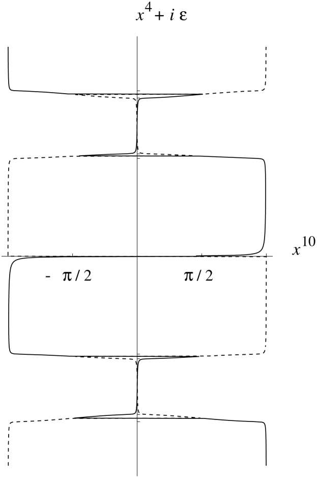
Figure 4: SO(4) imaginary part.

Figure 5: SO(5) with same values for the moduli as for SO(4) in Fig.4

Figure 6: SO(5) imaginary part.

Figure 7: Sp(4) real part. This is the same for both the two-fold and four-fold cover curves.

Figure 8: Sp(4) imaginary part for the two-fold cover curve.

We can now identify the number and position of the cuts of $\Sigma$ with the number and positions of the D4-branes. More precisely, it is the cuts in the semiclassical, ten dimensional limit $\mu\rightarrow 0$, $R_{10}\rightarrow 0$ that are the D4-branes. Therefore, a requirement to have well defined D4-branes in ten dimensions is that each branch cut collapses to a point. Again using SU($n$) as an example, we see that in the $\mu\rightarrow 0$ limit the discriminant $\Delta=B_{n+1}^{2}(v)-4\mu$ becomes a perfect square, each pair of branch points degenerates to a point, the branch cut disappears and we recover Witten’s description of the position of the D4-branes as the zeroes of $B_{n+1}(v)$. The same thing happens for all other classical groups as well. This can be seen by examining their $\Delta$’s listed in the following table: group $G$ $\Delta$ # cuts = $\frac{1}{2}$# b.p. genus of $\Sigma$ SU($n+1$) $B_{n+1}(v)^{2}-4\mu$ $n+1$ $n$ SO($2n$) $B_{n}(v^{2})^{2}-4\mu v^{4}$ $2n$ $2n-1$ SO($2n+1$) $B_{n}(v^{2})^{2}-4\mu v^{2}$ $2n$ $2n-1$ Sp($2n$) $B_{n}(v^{2})(v^{2}B_{n}(v^{2})-2\mu)$ $2n+1$ $2n$ However, as we will see in section 6 the behaviour of the exceptional curves in this limit is very different.

3.1 Multiple NS5-branes and product gauge groups

When $F(t,v)$ is of second order in $t$ identifying how the sheets combine to form NS5-branes was rather straightforward. The only subtlety being that the five branes should not “cross” each other in the $x^{6}$-direction at the branch points to avoid confusion on which brane is on the left and which on the right.

For higher number of NS5-branes the situation is more complicated: we can always determine the number of sheets and number of cuts, but trying to identify which sheets are connected by which cuts depends crucially on how we choose the phases at each cut. Take for example the three-fold cover curve that describes the product group ${\rm SU}(n)\times{\rm SU}(m)$ with bi-fundamental matter (see Fig. 9 for $n=m=2$):

$$t^{3}+t^{2}\left(B_{n}(v)+\frac{\mu_{m}}{\mu_{n}}\right)+t\left(B_{m}(v)\frac{\mu_{m}}{\mu_{n}}+\mu_{n}\right)+\frac{\mu_{m}^{2}}{\mu_{n}}=0,$$

here $\mu_{j}$ is the scale of SU($j$) gauge group.

Figure 9: SU(2)$\times$SU(2) with bi-fundamental matter

The branch points are still of second order (they connect only two sheets), but choosing the phases in a globally consistent way can be somewhat complicated. However, there is an additional piece of information we can use, namely the asymptotic behaviour of the sheets as $v\to\infty$. Looking at the curve for large, small and middle values of $t$ we see that they behave as $\ln v^{2},\ \ln v^{-2}$ and constant at large $v$. This means that the effective number of four-branes attached to each five-brane should be $2,-2$ and 0, respectively, where D4-branes on the left count as positive and on the right as negative. The classical limit now corresponds to taking $\mu_{n},\mu_{m}\to 0$ separately for each group. In other words we first decouple for example the second factor by $\frac{\mu_{n}}{\mu_{m}}\to\infty$, giving $\Delta\sim B_{n}(v)^{2}-4\mu_{n}$, and then take $\mu_{n}\to 0$ to localize the D4-branes at the zeroes of $B_{n}(v)$. Similarly for the SU($m$) factor. This reduces the curve to the usual ten dimensional brane configuration of a product of groups, studied for example in [27].

Before examining other gauge groups in detail we will discuss the role of the symmetries of the curves and how they will translate to orientifolds in the brane pictures.

4 Symmetries and Orientifolds

In most cases the curves given by the Toda-system have genus much higher than the rank of the group — only for SU($n+1$) with Lax-matrix in the fundamental representation do they agree. So in addition to finding the differential $\lambda_{SW}$, one needs to choose rank$(G)$ $\alpha$ and $\beta$-cycles and thus pick out the physically relevant rank$(G)$-dimensional subvariety of the Jacobian [14]. This sub-variety is called the preferred Prym. It is the same for all curves that correspond to the same gauge group, regardless of the representation of the Lax-matrix. Also, the curves have natural Weyl group actions acting on them. This induces symmetries on the cycles and differentials and therefore on the Jacobian. The preferred Prym variety is then the part of the Jacobian which corresponds to the reflection representation of the Weyl group.

For most gauge groups it is possible to find explicitly a genus $n$ curve for which the Jacobian is just the Prym variety. These curves are obtained from the original ones as quotients by certain symmetries, see for example [28] for explicit constructions. The physics of the $N=2$ SW gauge theory for the quotient curve is the same as the for the original curve.

It is natural to assume that the ten-dimensional brane picture should inherit the symmetries of the curve we wrap the M5-brane on. Because the symmetries originate from the Weyl group action we should see that action on the brane diagram. For SU($n+1$) this does not give us anything new: the curve already has genus $n$ and the Weyl group acts by permuting the D4-branes. But for other gauge groups we can use this to determine what the brane configuration should be.

The curves of orthogonal and symplectic groups have only ${{\sf Z\kern-3.99994ptZ}}_{2}$ symmetries. The SO($2n$) and Sp($2n$) curves (2) are both invariant under the involutions

$$\sigma_{1} : \quad v\to-v$$ (4)

$$\sigma_{2} : \quad t\to\mu/t.$$

Sp($2n$) has also an additional symmetry

$$\sigma_{3}:\quad t\to-t.$$

SO($2n+1$) curve on the other hand is left invariant only under $\sigma_{2}$ and the combination $\sigma_{1}\sigma_{3}$. If we rescale $t$ by

$$t=\sqrt{\mu}\exp[-(x^{6}+{\mathrm{i}}x^{10})/R\,]$$ (5)

we see that $\sigma_{2}$ corresponds to $x^{6}\to-x^{6},\ x^{10}\to-x^{10}$ and $\sigma_{3}$ to a shift in $x^{10}$ coordinate: $x^{10}\to x^{10}+{\mathrm{i}}\pi R$. These symmetries can be implemented to the ten dimensional brane diagrams by adding an orientifold [29]. There are two possibilities: either an O4-plane acting on the coordinates as

$$O4:\quad(x^{4},x^{5},x^{7},x^{8},x^{9},x^{10})\to(-x^{4},-x^{5},-x^{7},-x^{8},-x^{9},-x^{10})$$ (6)

or an O6-plane

$$O6:\quad(x^{4},x^{5},x^{6},x^{10})\to(-x^{4},-x^{5},-x^{6},-x^{10}).$$ (7)

The action of the O6 in the $v$ and $s$ coordinates is exactly the combined symmetry $\sigma_{1}\sigma_{2}$, whereas the O4 acts only as $\sigma_{1}$. With only two NS5-branes there is not much difference whether we will us an O4 or an O6, but with more then two NS5-branes there are problems associated to the charge of the O4 — it should change sign whenever the orientifold passes a five-brane [29]. Moreover, if we require that the orientifold projection should be equivalent to taking the quotient with respect to all the symmetries of the curve we find that the O6 is more natural.

4.1 Orientifold planes in M-theory

The reason why the O6 symmetries are related to the symmetries of the curves becomes more clear when we look at their eleven dimensional origin — they are certain types of singularities in M-theory [30, 32, 31]. Away from the singularity the complex structure of these spaces can be given by

$$xy=\mu v^{2k},$$ (8)

where $2k$ is the RR-charge of the orientifold and $\mu$ the parameter that sets the gauge theory scale: $\mu\sim\Lambda^{2h^{\vee}_{\bf g}}$; $x,y\sim\Lambda^{2h^{\vee}_{\bf g}+k}$. When the charge $2k$ is negative (8) describes a complex structure of the Atiyah-Hitchin space. The interpretation for the positive charge is less clear. Recall that adding to the gauge theory hypermultiplets in the fundamental representation corresponds to modifying the singularity structure by introducing $D6$-branes:

$$xy=\Lambda^{2h^{\vee}_{\bf g}}v^{2k-N_{f}}\prod_{i}^{N_{f}}(v-m_{i}).$$ (9)

Thus the positively charged O6 resembles $k$ D6-branes stuck in the origin, but with a singularity that can not be resolved.

The gauge theory curves of classical groups can now be described by the following equations:

$$\begin{array}[]{rll}{\rm SU}(n+1):&x+y-P_{n+1}(v)=0,&2k=0\\ {\rm SO}(2n):&x+y-P_{2n}(v^{2})=0,&2k=4\\ {\rm SO}(2n+1):&x+y-P_{2n}(v^{2})=0,&2k=2\\ {\rm Sp}(2n):&(x+y)^{2}-P_{2n}(v^{2})=0,&2k=-2\\ \end{array}$$ (10)

After using (8) to solve for $x$ and defining $y=tv^{k}$ we get the curves listed in (2). Note that here the SO($2n+1$) curve is symmetric under $v\to-v$, only the scaling of $y$ changes that. Also, the charge of the orientifold is not absolutely determined. For SO($2n+1$) we could as well have written $2k=4$ and $x+y-vP_{2n}(v^{2})=0$.

5 Orthogonal and Symplectic Groups

The brane diagram for SO($2n$) is easily determined. As we have seen, the symmetries of the curve are exactly those of O6. The ten dimensional configuration of branes consists of two NS5-branes, an orientifold six-plane in the origin and $2n$ D4-branes symmetrically on each side of $x^{6}$-axis. In addition, we see from Figure 4 that the NS5-branes extend to infinity in the $x^{4}$ due to bending caused by the orientifold. Those can be interpreted as two semi-infinite D4-branes on each side, located at $x^{4}=0$. The O6-plane effectively mods out all the symmetries, leaving only the physically significant part. In the original curve ${\cal C}_{{\rm SO}(2n)}:v^{2}(t+\mu/t)+P_{2n}(v^{2})=0$ this amounts to defining new variables $u=v(t-\mu/t)$ and $\xi=v^{2}$, giving the genus $n$ surface where the Prym lives:

$${\cal C}^{\prime}_{{\rm SO}(2n)}:\quad\xi u^{2}=P_{n}(\xi)^{2}-4\mu\xi^{2}.$$ (11)

Note that we can not wrap the M-theory five-brane directly on this reduced curve and still get the same world volume gauge theory. The reason is that to get the correct gauge group we need the orientifold to project out part of the Chan-Paton factors.

The SO($2n+1$) is a bit more complicated. As mentioned in the previous section, there are two equivalent descriptions: one with O6 of charge $2k=2$ and ${\cal C}_{{\rm SO}(2n+1)}:v(t+\mu/t)-P_{2n}(v^{2})=0$ and the other with a charge 4 orientifold and slightly different polynomial ${\cal C}_{{\rm SO}(2n+1)}:v^{2}(t+\mu/t)-vP_{2n}(v^{2})=0$. The former would describe a brane diagram with one semi-infinite D4-brane on each side of the five-branes at $v=0$ and nothing between them. The latter has also an extra D4-brane sitting on top of the orientifold, extending all the way to plus and minus infinity. So effectively this is the same as the SO($2n$) configuration but with one D4 in the origin $v=0$, between the five-branes, making it a total of $2n+1$ D4-branes. This is the configuration suggested also in [8]. In both cases, as for SO($2n$), the semi-infinite branes do not represent matter but are a result of the bending of the M5-brane in the presence of the orientifold. The genus $n$ quotient curve is very similar to that of SO($2n$):

$${\cal C}^{\prime}_{{\rm SO}(2n+1)}:\quad\xi y^{2}=P_{n}(\xi)^{2}-4\mu\xi,$$ (12)

where $y=t-\mu/t$ and $\xi=v^{2}$.

The Sp($2n$) curve differs from the curves of all other classical groups in that it is of fourth order in $t$, meaning that we should have a brane configuration with four NS5-branes. However, looking at the symmetries of and restricting to the physically significant part we can argue that only two NS5-branes are needed in ten dimensions.

Recall that the curve had an additional symmetry $\sigma_{3}:t\to-t$. Because this leaves the curve intact the effective period of $x_{10}$ is $2\pi\tilde{R}=\pi R$. Therefore instead of $t$ we should use

$$\tilde{t}=\mu\exp(-(x^{6}+{\mathrm{i}}x^{10})/\tilde{R})=t^{2}$$

as the variable of the curve. This gives

$${\tilde{t}}+\mu^{2}/{\tilde{t}}+2\mu-v^{2}P_{2n}=0,$$ (13)

where the remaining symmetries $\sigma_{1}$ and $\sigma_{2}$ can be realized as the action of an O6. Taking the quotient with respect to these gives the genus $n$ curve:

$${\cal C}^{\prime}_{{\rm Sp}(2n)}:\quad r^{2}=\xi P_{n}(\xi)(\xi P_{n}(\xi)-4\mu),$$

where $r={\tilde{t}}-\mu^{2}/{\tilde{t}}$. This curve is hyperelliptic, unlike the one we started from.

Solving the Sp($2n$) curve (2) for $\tilde{t}$ we get,

$$\tilde{t}=\frac{1}{2}\left[v^{2}P_{n}(v^{2})-2\mu\pm v\sqrt{P_{n}(v^{2})(v^{2}P_{n}(v^{2})-4\mu)}\,\right].$$

The point at $v=0$ is not a branch point. Even though there is only one solution at that point, $\tilde{t}=-\mu$, going around it does not produce a jump in the phase. This implies that there is no wrapping around the $x_{10}$ direction and therefore no D4-brane. At this point the curve is singular since $\partial F(v,\tilde{t})/\partial v|_{v=0}=\partial F(v,\tilde{t})/\partial\tilde{t}|_{\tilde{t}=-\mu}=0$. Thus, the two sheets will be connected at $v=0$ but this does not correspond to a dynamical D4-brane but to a singularity of the curve. But there are still $2n+1$ branch cuts. The one on the middle (see Fig. 8) comes from the factor $(v^{2}P_{n}(v^{2})-2\mu)$ and will in the $\mu\to 0$ limit collapse to a D4-brane stuck in the origin. This differs from the straightforward interpretation of the zeroes of the polynomials as the positions of the branes, which would give either $2n+2$ D4-branes, none of them at the origin, or $2n$ branes plus two branes on the origin. For the latter case, however, one needs to take a curve that does not come from the integrable system [8].

As for SO($2n+1$) we could have gotten the two-fold cover curve (13) for Sp($2n$) directly from the M-theory curves (10) by choosing a differently charged orientifold $2k=-4$ and another polynomial $x+y-P_{2n}(v^{2})+2\mu v^{-2}=0$. But then $x$ and $y$ would scale like $\Lambda^{2h^{\vee}_{g}-2}$ and we would need to introduce the term $2\mu v^{-2}$ by hand. Therefore we think that the Sp($2n$) curves in M-theory must be of second order in $x,y$ and consequently of fourth order in $t$, but the corresponding ten-dimensional brane diagram can be described with only two NS5-branes.

6 Branes and the Curves for G₂ and E₆

Now we can proceed to wrap the M-theory five brane on the Toda curve of exceptional groups and use the techniques developed in the previous sections to investigate what happens in the ten dimensional limit. We will study G₂ in detail and after that make brief comments on E₆.

6.1 G₂

The G₂ curve is

$${\cal C}_{{\rm G}_{2}}:\quad 3[t+\mu/t]^{2}+2v^{2}A_{2}(v^{2})[t+\mu/t]-v^{2}B_{6}(v^{2})-12\mu=0,$$ (14)

where $A_{2}(v^{2})=u_{2}-3v^{2}$ and $B_{6}(v^{2})=v^{6}-2u_{2}v^{4}+u_{2}^{2}v^{2}-u_{6}$. It has genus 11 and it is of fourth order in $t$. Unlike for Sp($2n$) there apparently is no symmetry that would allow us to find a two fold cover curve which is equivalent from the ten dimensional point of view. To see this, we first find the quotient curve ${\cal C}^{\prime}_{{\rm G}_{2}}$ that contains the Prym variety.

The obvious symmetries of ${\cal C}_{{\rm G}_{2}}$ are $\sigma_{1}$ and $\sigma_{2}$ in (4). We could obtain a double cover curve by taking the quotient with respect to these, but the resulting curve has genus one — too small to contain the Prym. There is a third symmetry though:

$$\sigma_{\mathrm{G}}:\quad t+\mu/t\to-[t+\mu/t+\frac{2}{3}v^{2}A_{2}(v^{2})].$$ (15)

Therefore, good variables are the ones invariant under the combined action of $\sigma_{1}$, $\sigma_{2}$ and $\sigma_{\mathrm{G}}$:

$$\xi=v^{2},\quad z=v[t+\mu/t+\frac{1}{3}v^{2}A_{2}(v^{2})].$$ (16)

They give a genus two curve [28]

$${\cal C}^{\prime}_{{\rm G}_{2}}:\quad 9z^{2}-\xi\left(3\xi B_{3}(\xi)+\xi^{2}{A_{1}}^{2}(\xi)+36\mu\right)=0$$ (17)

which is hyperelliptic even when the original curve was not. This curve is not the same as the hyperelliptic curve proposed for G₂ in [33, 34], whose physical validity was later questioned in [35]. Furthermore, it can be checked that the discriminant of the reduced curve $\Delta_{{\cal C}^{\prime}}$ is the same as the quantum discriminant $\Delta_{q}$ of G₂ field theory calculated in [35]:

$$\Delta_{q} =\mu\Delta_{-}^{2}\Delta_{+}^{2}$$ (18)

$$\Delta_{\pm} =-4u_{6}{u_{2}}^{3}+27{u_{6}}^{2}\mp 32{u_{2}}^{4}\sqrt{\mu}\pm 216u_{2}u_{6}\sqrt{\mu}-144{u_{2}}^{2}\mu\mp 6912\mu^{3/2}.$$

It does differ from the discriminant of the original four-fold cover curve ${\cal C}_{{\rm G}_{2}}$

$$\Delta_{{\cal C}}=\mu({u_{6}}^{2}-16{u_{2}}^{2}\mu)\Delta_{-}^{3}\Delta_{+}^{3}$$

by a prefactor, which was argued in [35] to correspond to an unphysical singularity.

In the previous section we saw that for Sp($2n$) the original spectral curve is also of fourth order in $t$ but it has a symmetry $t\to-t$ which allows us to define $\tilde{t}=t^{2}$. This is equal to a rescaling of the period of the eleventh coordinate $x^{10}$ and thus will not show in the ten dimensional brane diagram. Clearly, considering the symmetries of the G₂ curve, no scaling of $x^{10}$ will able us to find a two fold cover equivalent to (14). So if we want to construct a brane diagram for this theory it would have to originate from the four fold cover curve ${\cal C}_{{\rm G}_{2}}$ and therefore have four NS5-branes. We are going to investigate whether such a configuration makes sense and if it does not, why. Also, we want to understand how it would differ from the brane configurations for product gauge groups.

The branch points of the curve are located at the zeroes of

$$P_{8}(v)=3B_{6}(v)v^{2}+A_{2}(v)^{2}v^{4}+36\mu=0$$ (19)

and $v^{2}[3B_{6}(v)+2v^{2}A_{2}(v)^{2}\pm 2A_{2}(v)\sqrt{P_{8}(v)}\,]=0$, which is equivalent to

$$v^{2}P_{6}^{\pm}(v)=v^{2}[B_{6}(v)\pm 4\sqrt{\mu}\,A_{2}(v)]=0.$$ (20)

Note that as for Sp($2n$) the $v=0$ is not a branch point but a singularity of the curve. The two sets of branch points have very different characteristics. The global behavior of the cuts is a complicated issue. Fortunately, for our purposes it suffices to study some general features.

We now solve (14) for $t$ as a function of $v$ and label the sheets $t_{1},t_{2},t_{3}$ and $t_{4}$. For any point $v_{0}$ satisfying $P_{8}(v_{0})=0$ we see that $t_{1}(v_{0})=t_{2}(v_{0})$ and $t_{3}(v_{0})=t_{4}(v_{0})$. Therefore, for each pair of branch points coming from (19) there will be one tube connecting the $t_{1}$ and $t_{2}$ sheets and a second tube connecting the $t_{3}$ and $t_{4}$ sheets at the same value of $v=v_{0}$, giving a total of eight cuts (see Figure 10).

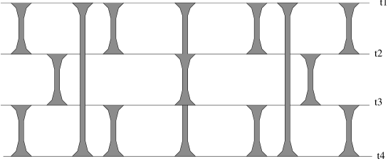
Figure 10: G₂ curve as a four fold cover of the $v$ plane.

The branch points satisfying (20) give rise to six branch cuts that join either $t_{1}$ and $t_{4}$ ( $P_{6}^{-}(v)=0$) or $t_{2}$ and $t_{3}$ ( $P_{6}^{+}(v)=0$ ). Unlike the previous case each cut corresponds to only one tube joining a pair of sheets.

If we identify the cuts with D4-branes we immediately see why this configuration is different from a product group: for product groups the positions of branes between different pairs of NS5-branes are not related. The D4-branes between the $k^{th}$ and the $(k+1)^{th}$ NS5-branes are free to move independently of the position of the branes between the $(k+1)^{th}$ and the $(k+2)^{th}$ NS5-brane. For the G₂ four fold cover for any value of the moduli the branch cuts between $t_{1}$ and $t_{2}$ have to be located at the same $(x^{4},x^{5})$ position as the cuts connecting $t_{3}$ and $t_{4}$. A similar thing happens for the brane configuration of SO($2n$) with matter in the symmetric representation [9], as a result of the orientifold six-plane in the middle. Moreover, because G₂ has only two moduli the positions of $P_{8}$-cuts depend in some way on the positions of the cuts that originate from $P_{6}^{\pm}$. Even classically, if we follow the prescription of identifying the number of branes with zeroes of the polynomials, we run into trouble. We would obtain a configuration with four NS5-branes, three D4-branes in the outermost columns and eight in the middle one. Seemingly, this describes a theory with ${\rm Sp}(2)\times{\rm SO}(8)\times{\rm Sp}(2)$ gauge group, but the curve only contains two moduli and one scale, $\mu$, and therefore can not describe a product gauge group.

A serious complication is that not all the cuts collapse to points when we go to ten dimensions, which was the requirement of having a well defined classical ten dimensional limit. All the cuts coming from the polynomials $P^{\pm}_{6}$ (20) and one cut from (19) have the desired behaviour when $\mu\to 0$, but the remaining three cuts do not. Therefore it seems that starting from the curve (14) it is not possible to get a ten dimensional brane configuration with G₂ field theory on the world volume.

If we try to construct a curve such that at least the discriminant would have same zeroes as the discriminant of the G₂ field theory, and also would have a well defined ten dimensional limit we will also encounter problems. For example, consider

$$2A_{2}(v^{2})v^{2}(t+\mu/t)-B_{6}(v^{2})=0,$$ (21)

which amounts to sending the outermost NS5-branes to infinity. The branch points are at $P_{6}^{-}P_{6}^{+}=0$ and the discriminant of the curve is $({u_{6}}^{2}-16{u_{2}}^{2}\mu)\Delta_{-}\Delta_{+}$. Now the cuts will collapse to points, creating a brane configuration with two NS5-branes and six four branes between them, four semi-infinite D4-branes on each side (two of them located at $v=0$) and an O6 in the middle. The semi-infinite branes do not generate hypermultiplets since there are no free moduli associated to any of them. The discriminant is the correct G₂ discriminant, modulo an unphysical factor, but we cannot obtain the G₂ Prym from it. The Jacobians of the new curve and ${\cal C}_{{\rm G}_{2}}$ can not be the the same because there is no way of getting the correct genus two curve from (21) by taking the quotient with respect to the symmetries — ${\cal C}^{\prime}_{{\rm G}_{2}}$ in (17) depends only on the polynomial $P_{8}(v)$, not on $P_{6}^{\pm}$. Therefore, even if this brane configuration does have some of the characteristics of a G₂ it can not contain all the information needed. We interpret these findings as an indication that it is not possible to have a weakly coupled Type IIA brane configuration that will reproduce a G₂ gauge theory.

Nevertheless, in the spirit of our previous examples we would like to implement the symmetries directly in M-theory to isolate the physically significant part of the curve. In order to get the correct gauge groups in the D4 world-volume gauge theory one has to project out part of the Chan-Paton degrees of freedom. For all other groups we have studied so far these projections were equivalent to modding out the symmetries of the curve, to find the genus $n$ part that contains the Prym. For G₂ the symmetries $\sigma_{1}$ and $\sigma_{2}$ can be realized as an O6, but since this gives a curve with genus one instead of two, it is not enough. We would need to implement also the new symmetry (15).

The transformation $\sigma_{\mathrm{G}}$ does square to identity, but it does not admit an interpretation as an orientifold plane in terms of the coordinates $t$ and $v$. In order to realize this symmetry we would need not an orientifold plane but a more complicated object in M-theory, which would live in the invariant locus $t+\mu/t+\frac{1}{3}v^{2}A_{2}(v)=0$ of the transformation $\sigma_{\rm G}$. This seems to be a kind of curved orientifold surface. After a coordinate transformation to $z$ defined in (16) $\sigma_{\rm G}$ reads $\frac{z}{v}\to-\frac{z}{v}$, which is the symmetry of an ordinary orientifold plane. However, after this transformation the O6 plane which corresponds to symmetries $\sigma_{1},\sigma_{2}$ will turn into a curved surface. It would be interesting to see if it is possible to construct a M-theory background, like the Atiyah-Hitchin space for O6, that would realize all the symmetries $\sigma_{2},\sigma_{2}$ and $\sigma_{\rm G}$ simultaneously.

6.2 E₆

The E₆ curve presents many of the characteristics seen in G₂. It is a genus 34 curve that can be realized as a four-fold cover of the $v$-plane (2). The branch cuts of the curve have the same behavior as in the G₂ case. Namely, they do not collapse to points when compactifying ten dimensions and thus will not describe D4-branes in this limit.

One of our original motivations was to examine the breaking of exceptional groups to get matter in the spinor representation. It is perfectly possible to take a curve, write the invariants $u_{i}$ of the bigger group in terms of the moduli of the group that it breaks into (for explicit construction for $E_{6}\to SO(10)\times U(1)$ see [37]) and recover in some limit of the moduli space a new curve which describes a group with a specific matter content. Unfortunately, as we have argued, there is no guarantee that the resulting curve will have a good limit in weakly coupled Type IIA theory.

For E₆ it is not known if a genus six curve that contains the Prym-Tjurin [28, 38] variety can be constructed explicitly. Thus, we can only speculate that even more complicated object than a curved orientifold would be needed in M-theory in order to obtain this subvariety.

7 Conclusions

We have seen that in the brane configurations for classical groups we can generically identify D4-branes with branch cuts of the Seiberg-Witten curve $\Sigma$. The need to introduce O6 or O4-planes to the brane configuration can be understood as the symmetries that have to be quotioned out in order to obtain the physically significant curve that has the Prym variety as its Jacobian.

We found several ways how the G₂ Toda curve differs from those of the classical groups. It does not have a well defined classical ten dimensional limit that would reduce the cuts to D4-branes. We think it is not possible to find a brane configuration in weakly coupled Type IIA string theory which would describe a G₂ field theory on the D4 world-volume. The situation for E₆ is similar and even more complicated.

Moreover, the symmetries of the G₂ curve can not be realized as orientifold planes. Instead we would need, in addition to an O6 plane, a curved orientifold surface. It would be interesting to see if it is possible to construct an M-theory background that would realize all the symmetries of G₂ simultaneously.

Acknowledgements

We would like to thank Eric D’Hoker, Jacques Distler and Sergey Cherkis for useful conversations and comments. E.C. thanks the Theory Group of UT Austin and P.P. the TEP Group in UCLA for their hospitality. The work of P.P. is supported by NSF grant PHY-9511632 and the Robert A. Welch Foundation and the work of E.C. by NSF PHY-9531023.

References

- [1] A. Hanany and E. Witten, Type IIB Superstrings, BPS Monopoles, and Three-Dimensional Gauge Dynamics, Nucl. Phys. B492 (1997) 152, hep-th/9611230.
- [2] E. Witten, Solutions of Four-Dimensional Field Theories Via M Theory, Nucl. Phys. B500 (1997) 3, hep-th/9703166
- [3] J. L. F. Barbón, Rotated Branes and Duality, Phys. Lett. 402B (1997) 59, hep-th/9703051
- [4] E. Witten, Branes and the Dynamics of QCD, Nucl. Phys. B507 (1997) 658, hep-th/9706109
- [5] S. Elitzur, A. Giveon, D. Kutasov, E. Rabinovici, A. Schwimmer, Brane Dynamics and N=1 Supersymmetric Gauge Theory , Nucl. Phys. B505 (1997) 202, hep-th/9704104
- [6] A. Giveon and D. Kutasov, Brane Dynamics and Gauge Theory , hep-th/9802067
- [7] K. Landsteiner, E. Lopez and D.A. Lowe, N=2 Supersymmetric Gauge Theories, Branes and Orientifolds, Nucl. Phys. B507 (1997) 197, hep-th/9705199
- [8] A. Brandhuber, J. Sonnenschein, S. Theisen and S. ‘Yankielowicz, M Theory and Seiberg-Witten Curves: Orthogonal and Symplectic Groups, Nucl. Phys. B504 (1997) 175, hep-th/9705232
- [9] K. Landsteiner and E. Lopez, New Curves from Branes, Nucl. Phys. B516 (1998) 273, hep-th/9708118
- [10] K. Dasgupta, S. Mukhi, F-theory at constant coupling, Phys. Lett. B385B (1996) 125, hep-th/9606044
- [11] A. Johansen, A comment on BPS states in F-theory in 8 dimensions, Phys. Lett. B395B (1997) 36, hep-th/9608186
- [12] M. Gaberdiel, B. Zwiebach, Exceptional Groups from Open Strings, Nucl. Phys. B518 (1998) 151, hep-th/970913
- [13] M. Gaberdiel, B. Zwiebach, Tensor Constructions of Open String Theories 1: Foundations, Nucl. Phys. B505 (1997) 569, hep-th/9705038
- [14] E. Martinec and N. P. Warner, Integrable Systems and Supersymmetric Gauge Theory, Nucl. Phys. B4 (5) 9199697, hep-th/9709161
- [15] W. Lerche and N. P. Warner, Exceptional SW Geometry from ALE Fibrations, Phys. Lett. 423B (1998) 79, hep-th/9608183
- [16] P. Pouliot, Chiral Duals of Non-Chiral SUSY Gauge Theories, Phys. Lett. 359BB (1995) 108, hep-th/9507018
- [17] M. Berkooz, P. Cho, P. Kraus, M.J. Strassler, Dual Descriptions of SO(10) SUSY Gauge Theories with Arbitrary Numbers of Spinors and Vectors, Phys. Rev. DD56 (1997) 7166, hep-th/9705003
- [18] A. Klemm, W. Lerche, P. Mayr, C. Vafa, N. Warner, Self-dual Strings and N=2 Supersymmetric Field Theory, Nucl. Phys. B477 (1996) 746, hep-th/9604034
- [19] H. Itoyama and A. Morozov Integrability and Seiberg-Witten theory: Curves and Periods Authors: H. Itoyama, A. Morozov, Nucl. Phys. B477 (1996) 855, hep-th/9511126
- [20] A.Gorsky, I.Krichever, A.Marshakov, A.Mironov, A.Morozov, Integrability and Seiberg-Witten Exact Solution , Phys. Lett. 355B (1995) 466, hep-th/9505035
- [21] E. J. Martinec and N. P. Warner, Integrability and N=2 Gauge Theory : A Proof, hep-th/9511052
- [22] E. D’Hoker and D.H. Phong, Calogero-Moser Systems in Seiberg-Witten Theory, Nucl. Phys. B513 (1998) 405, hep-th/9709053
- [23] R. Donagi and E. Witten, Supersymmetric Yang-Mills Systems And Integrable Systems, Nucl. Phys. B460 (1996) 299, hep-th/9510101
- [24] C. Ahn, K. Oh, R. Tatar Sp(N) Gauge Theories and M Theory Fivebrane, hep-th/9708127
- [25] C. Ahn, K. Oh, R. Tatar, M Theory Interpretation for Strong Coupling Dynamics of SO(N) Gauge Theories, Phys. Lett. 416B (1998) 75, hep-th/9709096
- [26] C. Ahn, K. Oh and R. Tatar, Comments on SO/SP Gauge Theories from Brane Configurations with an O(6) Plane, hep-th/9803197
- [27] J. Erlich, A. Naqvi and L. Randall, The Coulomb Branch of N=2 Supersymmetric Product Group Theories from Branes, hep-th/9801108
- [28] R. Donagi, Seiberg-Witten integrable systems, alg-geom/9705010
- [29] N. Evans, C.V. Johnson and A.D. Shapere, Orientifolds, Branes, and Duality of 4D Gauge Theories, Nucl. Phys. B505 (1997) 251, hep-th/9703210
- [30] N. Seiberg, IR Dynamics on Branes and Space-Time Geometry , Phys. Lett. 384B (1996) 81, hep-th/9606017
- [31] A. Sen, A Note on Enhanced Gauge Symmetries in M- and String Theory, J.High Energy Phys.9 (1997) 001, hep-th/9707123
- [32] N. Seiberg and E. Witten, Gauge Dynamics and Compactification to Three Dimensions, hep-th/9607163
- [33] M. Alishahiha, F. Ardalan, F. Mansouri, The Moduli Space of the Supersymmetric G(2) Yang-Mills Theory , Phys. Lett. 381B (1996) 446, hep-th/9512005
- [34] U. H. Danielsson and B. Sundborg, Exceptional Equivalences in N=2 Supersymmetric Yang-Mills Theory, Phys. Lett. 370B (1996) 83, hep-th/9511180
- [35] K. Landsteiner, J. M. Pierre and S. B. Giddings, On the Moduli Space of N = 2 Supersymmetric Gauge Theory , Phys. Rev. D55 (1997) 2367, hep-th/9609059
- [36] K. Ito, Picard-Fuchs Equations and Prepotential in N=2 Supersymmetric Yang-Mills Theory , Phys. Lett. 406B (1997) 54, hep-th/9703180
- [37] W. Lerche and N. P. Warner, Polytopes and Solitons in Integrable N=2 Supersymmetric Landau-Ginzburg Theories, Nucl. Phys. B358 (1991) 571
- [38] V. Kanev, Spectral Curves, Simple Lie Algebras and Prym-Tjurin Varieties , Proceedings of Symposia in Pure Mathematics, Vol. 49 (1989) 627