IASSNS-HEP-98/60

PUPT-1802

hep-th/9806214

Tachyons and Black Hole Horizons in Gauge Theory

Daniel Kabat¹ and Gilad Lifschytz²

¹School of Natural Sciences

Institute for Advanced Study

Princeton, New Jersey 08540, U.S.A.

kabat@ias.edu

²Department of Physics

Joseph Henry Laboratories

Princeton University

Princeton, New Jersey 08544, U.S.A.

gilad@puhep1.princeton.edu

Any probe which crosses the horizon of a black hole should be absorbed. In M(atrix) theory, for 0-brane probes of Schwarzschild black holes, we argue that the relevant absorption mechanism is a tachyon instability which sets in at the horizon. We give qualitative arguments, and some quantitative large-$N$ calculations, in support of this claim. The tachyon instability provides an attractive mechanism for infalling matter to be captured and thermalized by a Schwarzschild black hole.

June 1998

1 Introduction

It is natural to ask what M(atrix) theory [1] has to say about the physics of Schwarzschild black holes. Several groups have investigated this subject [2, 3, 4, 5, 6, 7, 8, 9, 10, 11, 12, 13]. By modeling the black hole as a Boltzmann gas of 0-branes, several key properties such as the entropy – mass relationship and the Hawking temperature have been derived, up to numerical coefficients of order unity.

But the defining property of a black hole in classical gravity is the existence of an event horizon. In this paper we address the question of how a horizon manifests itself in M(atrix) theory. One’s first thought – that the size of the horizon is given by the range of eigenvalues of the matrices ${\bf X}_{i}$ – cannot be correct, since this range is expected to diverge in the large $N$ limit for all states in M(atrix) theory.

In a scattering experiment the horizon area of a black hole can be measured from its absorption cross section. In the context of M(atrix) theory this reflects the fact that a probe 0-brane should be absorbed by the black hole once it crosses the horizon.

For Schwarzschild black holes in M(atrix) theory our proposal is that the mechanism responsible for this absorption is a tachyon instability: the probe 0-brane sees the horizon as a critical radius, at which strings stretched between the probe and the black hole become tachyonic. This provides a precise prescription for identifying the horizon in M(atrix) theory.

At a qualitative level, one can see that a state in gauge theory that gives rise to such a tachyon region will have the features expected of a black hole. Suppose a probe enters the tachyon region. Then the tachyons will start to condense, so the probe will be captured with very high probability. Moreover, the tachyonic modes couple to all the other degrees of freedom which make up the initial state, and the energy released as the tachyon condenses is available to be redistributed among all these degrees of freedom. Thus within the gauge theory we see that infalling matter gets absorbed and quickly thermalized when it enters a region with a tachyon instability. This is all directly analogous to the behavior expected of matter falling into a black hole.

Although our treatment will focus on 11-dimensional Schwarzschild black holes, we expect the discussion of tachyon instability to apply more generally to the horizon of non-extremal D-brane black holes, as well as to non-extremal black holes in the context of anti de Sitter space [14].

Extremal black holes must behave somewhat differently, however. A supersymmetric probe of an extremal black hole should still be absorbed when it reaches the horizon, but the mechanism cannot be a tachyon instability. In section 3 we will give a brief discussion of string pair creation as a possible mechanism in the extremal case.

An outline of this paper is as follows. In section 2 we review some facts about Schwarzschild black holes in M(atrix) theory and absorption mechanisms in D-brane scattering. In section 3 we argue that a tachyon instability, if present, would have the features expected of a Schwarzschild horizon in M(atrix) theory. In section 4 we study the tachyon instability for several explicit M(atrix) configurations. Although we cannot directly study black hole states, the examples we consider are sufficient to show that tachyons are indeed present in M(atrix) theory, in regions which can plausibly be associated with Schwarzschild horizons. Section 5 contains some conclusions.

2 Preliminaries

We review some relevant results concerning Schwarzschild black holes in M(atrix) theory and absorption mechanisms in D-brane scattering.

2.1 Schwarzschild black holes in M(atrix) theory

The most general object in M(atrix) theory is a collection of 0-branes with some strings stretching between them. The only truly stable states are the gravitons, but a black hole can be thought of as a long lived quasi-stable state. A Schwarzschild black hole has negative heat capacity, unlike any state in SYM. But in terms of light cone variables a black hole actually has a positive heat capacity if the number of non-compact dimensions is six or larger [3]. This makes it possible to be described using SYM.

Another feature of gravity that is relevant for black holes is that one can’t put an arbitrary amount of energy in a bounded region. The upper limit for a given region is the black hole mass with the horizon area chosen appropriately. In M(atrix) theory we can see a similar effect. Fix the size of the matrices at $N\times N$, and choose some volume with typical length $L$. We want to see if there is a limit on the SYM energy, with the restriction that the object is contained within the designated volume. This is easy to see at the classical level of the SYM. For the moment let us define the size to be at most the volume occupied by the eigenvalues of the matrices (which are not necessarily simultaneously diagonalizable). Now take nine diagonal matrices with some distribution of eigenvalues $-L<\lambda<L$. This state has zero energy. The most general configuration with these eigenvalues can be obtained by acting with different unitary matrices on each of the original nine matrices. As the magnitude of each entry of a unitary matrix is smaller than 1, there is a limit on the entries of the resulting nine matrices. Then it is clear that the energy $\sim{\rm Tr}[{\bf X}_{i},{\bf X}_{j}]^{2}$ is bounded.

Currently the best understood model for Schwarzschild black holes is at the so-called BFKS point, that is when $N\sim S$ [2]. At this point the temperature of the SYM is so low that quantum fluctuations are of the same order as thermal fluctuations. To go beyond this point, to $N\gg S$, requires a fully quantum mechanical treatment of the system. Following [2], one can model black holes with entropy $\sim N$ as follows. The basic ingredient is a state that has some expectation value for the matrices, $B_{i}=<{\bf X}_{i}>$ (this is referred to as the background). The SYM energy of this state is identified with the light-cone energy of the black hole, and the volume of the state is the volume of the black hole (we will come back to what we mean by volume of the state). The background and its fluctuations (which are modeled as a gas of N particles) contribute to the entropy and energy of the state. In fact most papers deal only with the thermodynamics of these fluctuations.

For the entropy to come out correctly it is crucial that the statistics of the fluctuations be that of distinguishable particles. This issue is somewhat subtle. If all the background matrices commute (so that they can be simultaneously diagonalized) then there is a residual gauge symmetry that permutes the diagonal elements, which makes the statistics that of identical particles. In this case the entropy is very small. To see this take a gas of free identical particles in $d$ dimensions. The assumed kinematics is that each particle has momentum $p_{\perp}\sim 1/R_{S}$ set by the uncertainty principle and mass $m=1/R$, where $R_{S}$ is the Schwarzschild radius and $R$ is the radius of the null circle. The volume of the gas is $V=\left(R_{S}\right)^{d}=N$ at the BFKS point. The energy of the gas is then $E\sim NR/R_{S}^{2}$. For a gas of $N$ distinguishable particles in $d$ space dimensions the entropy is

$$S=N\log\left[V\left(\frac{4\pi mE}{dN}\right)^{d/2}\right]+\frac{dN}{2}$$ (1)

This entropy is indeed $\sim N$. If the particles are identical then the volume $V$ would be replaced with $V/N$ and there would be very little entropy.

If the background matrices do not commute (which means that there is a coherent state of strings stretched between different 0-branes) then we no longer have the residual gauge symmetry discussed above and thus do not have identical particles. The factor $1/N$ will not appear and the entropy will be order $N$. But the parameter which breaks the statistics symmetry is continuous, and it is not entirely clear at what value the effective statistics actually changes. For instance, if the energy in the fluctuations is much larger than the energy of the background then it is not clear why the above analysis should apply.

Another issue is how to measure the size of a state. Clearly it cannot simply be the volume occupied by the 0-branes (although this will provide an upper bound) since, according to the holographic principle, this is expected to grow with $N$ even for a graviton [2]. The most physical measure of the size of a state is through scattering experiments. For a black hole, in particular, it is natural to use the absorption cross-section as a definition of the horizon size. So before applying this definition to M(atrix) black holes we briefly review absorption mechanisms in D-brane scattering.

2.2 Absorption in D-brane scattering

In D-brane scattering there are two mechanisms which contribute to the imaginary part of the phase shift and lead to absorption.

The first mechanism is string creation. When two D-branes have non-zero relative velocity, there is an amplitude to pair create two oppositely-oriented open strings stretched between them. Since velocity is T-dual to an electric field on the D-brane worldvolume, and open strings carry electric charge, this is dual to the phenomenon of pair production in an electric field [15].

In the scattering amplitude, string creation arises as follows. The one-loop eikonal phase shift for D0 – D0 scattering has the form ($b$ is the impact parameter and $v$ is the relative velocity) [16]

$$\delta(b,v)\sim\int_{0}^{\infty}\frac{ds}{s}e^{-b^{2}s/2\pi\alpha^{\prime}}\frac{f(s,v)}{\sin sv}$$ (2)

At $sv=n\pi$ the integrand has poles which contribute an imaginary part to the phase shift. The outgoing wavefunction of the scattered 0-brane is multiplied by $e^{i\delta}$. Significant string creation is possible only for $b<\sqrt{v\alpha^{\prime}}$, since for large $b$ the imaginary part is exponentially suppressed, ${\sl Im}\,\delta\sim e^{-b^{2}/v\alpha^{\prime}}$. This effect can be clearly seen in the SYM truncation of the one-loop amplitude, where the norm of the outgoing wavefunction is [16, 17]

$$|\psi|^{2}=\tanh^{8}\left(\frac{b^{2}}{4\alpha^{\prime}v}\right)\,.$$ (3)

Of course for string creation to be possible there must be enough kinetic energy in the first place. So we see that there are two requirements for significant string creation to be possible,

$$b<2\sqrt{v\alpha^{\prime}}\qquad\hbox{\rm and}\qquad b<2\pi\alpha^{\prime}{m_{s}\over 2g_{s}}v^{2}\,.$$ (4)

The second condition is the more stringent one when the relative velocity is small.

The second mechanism for absorption we refer to as tachyon instability [18]. While there is always a term $e^{-b^{2}s}$ in the integrand for the phase shift, it could happen that for large $s$ the function $f(s,v)$ behaves like $e^{+c^{2}s}$. In eikonal scattering this happens when the oscillator ground state energy of the stretched string is negative. Then for $b<c$ the proper time integral for the phase shift diverges. But by analytically continuing one sees that what actually happens is the phase shift acquires an imaginary part.

Once a tachyon instability develops, the tachyon field will tend to condense. In a sense this condensation can be viewed as string creation, since a coherent state of stretched strings is produced (the strings just happen to have negative energy). But this picture of tachyons as stretched strings can be somewhat misleading in M(atrix) theory. In the context of SYM calculations the tachyon instability arises when the (mass)² matrix for the off-diagonal elements has a negative eigenvalue. Of course the full potential ${\rm Tr}[{\bf X}_{i},{\bf X}_{j}]^{2}$ has a quartic piece that stabilizes the tachyon field at some finite value. When the tachyons condense, they lower the energy of the original configuration. They do this by making the off-diagonal elements larger, which naively means that additional strings are being added to the configuration. But after the tachyons condense, one can rediagonalize the matrices. One finds that the final configuration can be reinterpreted as having fewer stretched strings present than the initial state. Related phenomena have been discussed in string theory [19, 20].

In view of this ambiguity, we will use the term ‘string creation’ only in reference to the pair production of open strings with positive energy arising from poles in the integrand. A point which will be important is that, even if no tachyon is present, string creation is enhanced when $c^{2}$ is positive. This is because the requirements for string creation (4) are relaxed to have the form

$$b<\sqrt{4\alpha^{\prime}v+c^{2}}\qquad\hbox{\rm and}\qquad b<2\pi\alpha^{\prime}\left({m_{s}\over 2g_{s}}v^{2}+c\right)$$ (5)

Thus string creation becomes possible for a wider range of impact parameters when $c^{2}$ is positive.

3 Horizons in gauge theory

An essential feature of classical black holes is that they have an event horizon. That is, there is a region of spacetime from which one cannot escape back to future infinity. This means that classically once an object enters the horizon it will be absorbed with certainty.

We want to understand how this happens in gauge theory. In principle given the wave function of a black hole state in the gauge theory we could compute its absorption cross-section. This absorption could arise from one or both of the mechanisms discussed above. We first discuss Schwarzschild black holes, then briefly discuss the extremal case.

3.1 Schwarzschild black holes

To mimic the black hole, we expect absorption to set in at a relatively sharp radius, which should not depend on the nature of the probe. In particular the absorption cross section should be approximately independent of the incoming probe momentum. As we will see, this is a non-trivial requirement.

We first consider string creation as a possible mechanism, and ask whether string creation by gas of 0-branes (treated as distinguishable particles) can be responsible for absorption by a Schwarzschild black hole at the BFKS point. The criterion is that if we send in a probe 0-brane with transverse momentum $p_{\perp}$ at an impact parameter smaller than the Schwarzschild radius it should be absorbed. This depends on the mean free path of a 0-brane in the gas of 0-branes making up the black hole. The mean free path is given by

$$d=\frac{1}{n\sigma}$$ (6)

where $n$ is the number density of the gas and $\sigma$ is the absorption cross-section. To estimate $\sigma$ we use the string creation conditions (4). If the velocity is large then the absorption radius $b\sim\sqrt{v}$ and hence $\sigma\sim p_{\perp}^{4}$, while at small velocity $b\sim v^{2}$ so $\sigma\sim p_{\perp}^{16}$. The key point is that the probability of string creation vanishes as the relative velocity goes to zero.

The condition for absorption is that the mean free path be smaller than the Schwarzschild radius, $d<R_{S}$. Using the BFKS density $n\sim 1/l_{p}^{9}$ this translates into a lower bound on the transverse momentum of the probe. For large black holes it is the $\sigma\sim p_{\perp}^{16}$ estimate which controls the bound: a probe must have

$$p_{\perp}>(R_{S})^{-1/16}$$ (7)

in Planck units to be absorbed. This is rather unsatisfactory. It would indicate that a Schwarzschild black hole with radius $10^{38}l_{p}\sim 1.6{\rm km}$ can only absorb particles with momenta larger than $4\times 10^{-3}m_{p}\sim 10^{16}{\rm GeV}$.

This seems to rule out pure string creation as a mechanism for absorption by the black hole. But one can consider the following hybrid mechanism. Recall from (5) that, even if no tachyon develops, string creation is enhanced when the oscillator ground state energy of a stretched string is negative. Basically this makes the string lighter so it is easier to pair produce them. One could imagine that this enhances string creation to the point where it is responsible for absorption by the black hole.

Such an effect is very plausibly present in non-extremal M(atrix) black holes, as our examples in section 4 will show. But given that negative oscillator ground state energies are present and seem to play a significant role, it is natural to imagine that a full-blown tachyon instability might be present. So let us look more closely at the tachyon instability as an absorption mechanism.

Once a probe 0-brane enters the tachyon region, the tachyon mode will start to condense and roll down its potential. In the process it acquires kinetic energy. But the tachyon field is coupled non-linearly to the other degrees of freedom making up the black hole via the ${\rm Tr}[{\bf X}_{i},{\bf X}_{j}]^{2}$ interaction, so this energy is available for distribution among all black hole degrees of freedom. This is the process of absorbing and thermalizing the new matter that fell into the black hole.

One might worry that the probe 0-brane will leave the unstable region before the tachyon condenses. The time scale for the tachyon to start rolling down the potential is $t_{0}\sim 1/\sqrt{-m_{tachyon}^{2}}$. Unless the probe just grazes the horizon, in order not to be captured it must have a velocity of at least $v\sim R_{s}/t_{0}$. At such large velocities our quasistatic treatment of the background isn’t reliable, although we note that at very high velocities string creation could be an important effect. One also might worry that the energy which is released by tachyon condensation could eject one of the other 0-branes from the black hole. But this is very unlikely at large $N$, when there are many degrees of freedom present that can share the energy.

Of course 0-branes do escape from the black hole as Hawking particles [10]. It would be interesting to understand how the tachyon instability affects this process. Suppose a particular 0-brane is liberated, in that the strings connecting it to the rest of the black hole happen to fluctuate to zero (either thermally or quantum mechanically). If this happens inside the tachyon region, then it is still classically almost impossible for the 0-brane to escape the black hole. It is as if the 0-branes have to tunnel out of the tachyon region in order to escape.

Note that the tachyon instability does not depend sensitively on the relative velocity of the probe and target – it is an effective absorption mechanism even if the probe has zero velocity. The tachyon instability does depend crucially on the structure of the target, however, and it is plausible that it could distinguish graviton states (which do not have horizons) from Schwarzschild black holes (which do), even though holography dictates that both gravitons and black holes in a sense grow with $N$.

We feel that these properties make a tachyon instability an attractive mechanism for absorption by a Schwarzschild black hole. It seems natural to associate the tachyon region with the size of the black hole horizon. To make this plausible, we must show that tachyon instabilities can arise in macroscopically large regions in M(atrix) theory. We will do this in section 4 through consideration of some explicit examples.

3.2 Extremal black holes

When a D-brane is used to probe an extremal black hole, absorption should still set in at the horizon. But the physical mechanism for absorption must be different from the Schwarzschild case, since a (supersymmetric) probe can’t develop a tachyon instability.

An explicit example of such a system was studied in ref. [21]. These authors used a D1-brane to probe an extremal black hole with three charges, D1, D5, and momentum. One observation they made is that the horizon should be identified with the origin of the Coulomb branch of the probe gauge theory. They studied geodesic motion on this moduli space, and argued that certain geodesics which fall in towards $\rho=0$ are a signal of eventual absorption by the black hole.

Unlike Schwarzschild black holes, the mechanism responsible for absorption at the horizon of an extremal black hole cannot be a tachyon instability. Instead the mechanism is more plausibly one of string pair creation. Consider geodesic motion of a probe towards the origin of moduli space. The probe must have some non-zero velocity $v$. Then sufficiently close to the origin string creation will become possible and the moduli space approximation will break down. String creation gives rise to an absorptive part of the scattering amplitude, and can lead to capture of the probe by the black hole (in gauge theory terms a transition from the Coulomb to the Higgs branch). As discussed above, string pair creation has a slow rate of thermalization, since no energy is released in the process. But this is consistent with the black hole being extremal.

4 Examples of tachyon regions

In this section we calculate the tachyon instability region (TIR) in some explicit M(atrix) configurations. Ideally we would perform this calculation for states corresponding to gravitons and Schwarzschild black holes. But our lack of precise knowledge of these wavefunctions forces us to turn to some simpler examples, which we nonetheless feel point out some general features of the TIR. Our purpose is to make it plausible that tachyons are present in M(atrix) theory, in macroscopic regions that can be associated with Schwarzschild black holes.

The general calculational framework is as follows. We choose an $N\times N$ target configuration $B_{i}$, and place a 0-brane probe at a position $b_{i}$. This corresponds to a background in M(atrix) theory

$$<{\bf X}_{i}>=\left[\begin{array}[]{cc}B_{i}&0\\ 0&b_{i}\end{array}\right]\,.$$

The covariant gauge-fixed action of the M(atrix) quantum mechanics is [23]

$${\cal S} = \frac{1}{g_{YM}^{2}}\int dt\,{\rm Tr}\left(D_{t}{\bf X}_{i}D_{t}{\bf X}_{i}+\frac{1}{2}[{\bf X}_{i},{\bf X}_{j}]^{2}+i\Psi_{a}D_{t}\Psi_{a}-\Psi_{a}\gamma_{ab}^{i}[{\bf X}_{i},\Psi_{b}]\right)$$

$$\qquad\qquad+{\cal L}_{\hbox{\small gauge fixing}}+{\cal L}_{\hbox{\small ghost}}\,.$$

Expanding the action around the background to quadratic order gives the following (mass)² matrices for the off-diagonal degrees of freedom connecting the probe to the target (see for example [27]).

$$M^{2}_{\rm YM} = \left[\begin{array}[]{cc}\sum_{k}\left(B_{k}-b_{k}\right)^{2}&-2\partial_{t}\left(B_{j}-b_{j}\right)\\ \vskip 2.84526pt\cr 2\partial_{t}\left(B_{i}-b_{i}\right)&\hskip 2.84526pt\delta_{ij}\sum_{k}\left(B_{k}-b_{k}\right)^{2}+2[B_{i},B_{j}]\end{array}\right]$$ (10)

$$M^{2}_{\rm fermi} = \sum_{i}(B_{i}-b_{i})^{2}\otimes{\hbox to0.0pt{1\hss}\hskip 1.6pt\hbox{1}}_{16\times 16}+i\partial_{t}\left(B_{i}-b_{i}\right)\otimes\gamma^{i}+{1\over 2}[B_{i},B_{j}]\otimes\gamma^{ij}$$

$$M^{2}_{\rm ghost} = \sum_{i}(B_{i}-b_{i})^{2}$$

We want to identify the probe positions which give rise to at least one negative (mass)² eigenvalue. Clearly $M^{2}_{\rm ghost}$ is positive definite so we do not need to worry about the ghosts. As long as the background is static $M^{2}_{\rm fermi}$ is also the square of a Hermitian matrix and hence is positive definite. So tachyons do not arise in the fermion sector and we can ignore them as well.

This leaves the Yang-Mills degrees of freedom. If the background is time independent then $A_{0}$ does not mix with ${\bf X}_{i}$, and we only need to consider the following $9N\times 9N$ (mass)² matrix for the ${\bf X}_{i}$ degrees of freedom.

$$\left(M^{2}\right)_{ij}=\delta_{ij}\sum_{k}\left(B_{k}-b_{k}\right)^{2}+2[B_{i},B_{j}]$$ (11)

Even if the background does depend on time, dropping $A_{0}$ in this way sets a lower bound on the size of the region with tachyons: given an $n\times n$ Hermitian matrix with smallest eigenvalue $\lambda_{\rm min}$, deleting one row and one column of the matrix produces a new $(n-1)\times(n-1)$ matrix whose smallest eigenvalue is larger than $\lambda_{\rm min}$ [24]. So for the rest of the paper we will only analyze the mass matrix (11).

More generally, in situations where the target must be treated quantum mechanically, we can promote (11) to an operator equation. That is, we can promote the classical background $B_{i}$ to a $u(N)$-valued quantum operator ${\bf X}_{i}$, and write

$$\left(M^{2}\right)_{ij}=\delta_{ij}\sum_{k}\left({\bf X}_{k}-b_{k}\right)^{2}+2[{\bf X}_{i},{\bf X}_{j}]$$ (12)

where $[\cdot,\cdot]$ denotes the commutator in $u(N)$. A tachyon instability is present if the expectation value $<\psi|M^{2}|\psi>$ has a negative eigenvalue. This can be regarded as a proposal for defining the quantum horizon radius operator for a Schwarzschild M(atrix) black hole.

4.1 An $N=2$ example

We start by considering the case $N=2$. This is mainly a warm-up to illustrate some properties of the TIR. An interesting feature which will emerge is that the TIR does not have to be connected.

We consider backgrounds of the following form, involving two 0-branes and some stretched strings.

$${\bf X}_{1}(t) = a_{1}(t)\sigma^{3}$$ (13)

$${\bf X}_{2}(t) = a_{2}(t)\sigma^{1}$$ (14)

The $\sigma^{i}$ are Pauli matrices. In general the operators $a_{1}(t)$, $a_{2}(t)$ obey Heisenberg equations of motion, but for illustrative purposes we will assume that there is some classical time-independent background

$$B_{1} = a_{1}\sigma^{3}$$ (15)

$$B_{2} = a_{2}\sigma^{1}$$ (16)

that approximates the properties of the state we are interested in. The constants $a_{1}$, $a_{2}$ which appear in the background can be thought of as suitable time averages of quantum expectation values.

The mass matrix for the bosons has the form

$$M^{2}=\left(\begin{array}[]{cc}C&2D\\ -2D&C\end{array}\right)$$

where $C$ and $D$ are $2\times 2$ matrices.

$$C = (a_{1}^{2}+a_{2}^{2}+b_{1}^{2}+b_{2}^{2}){\hbox to0.0pt{1\hss}\hskip 1.6pt\hbox{1}}+2a_{1}b_{1}\sigma^{3}+2a_{2}b_{2}\sigma^{1}$$ (17)

$$D = 2ia_{1}a_{2}\sigma^{2}$$ (18)

We want to find the region in $(b_{1},b_{2})$ space where the probe has a tachyon instability, i.e. where $M^{2}$ has a negative eigenvalue. The boundary of this region can be found by looking for zeroes of the determinant. Without loss of generality we assume $a_{2}^{2}>a_{1}^{2}$, and find that the tachyon region is

$$0\leq b_{1}^{2}\leq\sqrt{12a_{1}^{2}a_{2}^{2}+4(a_{2}^{2}-a_{1}^{2})b_{2}^{2}}-a_{2}^{2}-b^{2}_{2}+a_{1}^{2}$$ (19)

$${\rm max}\left(0,a_{2}^{2}-a_{1}^{2}-\sqrt{12}a_{1}a_{2}\right)\leq b_{2}^{2}\leq a_{2}^{2}-a_{1}^{2}+\sqrt{12}a_{1}a_{2}$$ (20)

The maximum of $b_{1}^{2}$ is

$${\rm max}\left(\frac{3a_{1}^{2}a_{2}^{2}}{a_{2}^{2}-a_{1}^{2}},\sqrt{12}a_{1}a_{2}-a_{2}^{2}+a_{1}^{2}\right)$$ (21)

If $a_{1}=a_{2}$ then there is a tachyonic instability in a disk of radius $b^{2}=\sqrt{12}a_{1}^{2}$. If $a_{2}^{2}-a_{1}^{2}-\sqrt{12}a_{1}a_{2}>0$ then there are two distinct regions in which there is a tachyonic instability. If $a_{2}^{2}\gg a_{1}^{2}$ then the TIR consists of two regions, each roughly a circle of radius $\sim a_{1}$, centered at $(0,a_{2})$ and $(0,-a_{2})$.

To look more precisely at the imaginary part, let us compute the phase shift of a 0-brane scattered from this configuration. To simplify things we will take the impact parameter $b$ to be in the $x^{3}$ direction (and not as before in directions $x^{1}\,x^{2}$), and give the probe 0-brane velocity $v$ in direction $x^{4}$. In this case there is still string creation and a tachyonic instability so this simple example serves to illustrate the general case. Diagonalizing the (mass)² matrices (10) leads to the one-loop phase shift

$$\delta(b,v) = \int\frac{ds}{s}\,e^{-(b^{2}+a_{1}^{2}+a_{2}^{2})s}\frac{1}{\sin sv}\,(4+2\cosh 4a_{1}a_{2}s+2\cos 2sv$$

$$\qquad\qquad\qquad\qquad\qquad-8\cos sv\cosh 2a_{1}a_{2}s)$$

and there is a tachyonic instability for $b^{2}<4a_{1}a_{2}-a_{1}^{2}-a_{2}^{2}$. Notice that there is no tachyon in the fermionic sector (the last term in equation(4.1)). From equation (4.1) the norm of the outgoing wave function of the scattered 0-brane can be computed to give

$$|\psi_{out}|=\frac{(\cosh\frac{\pi r^{2}}{v}-\cosh\frac{\pi c}{v})^{4}}{8\cosh^{6}\frac{\pi r^{2}}{2v}(\cosh\frac{\pi r^{2}}{v}+\cosh\frac{2\pi c}{v})}$$ (23)

where we have put $r^{2}=b^{2}+a_{1}^{2}+a_{2}^{2}$ and $c=2a_{1}a_{2}$. Let us look at equation (23). If $a_{2}=0$ then we are reduced to scattering one 0-brane from two other 0-branes with the usual answer of $\tanh^{8}\left(\pi b^{2}/v\right)$. In the small $v$ limit if $r^{2}<4a_{1}a_{2}$ the norm of the wave function is $\sim 0$. Furthermore, even for small $v$ and $r^{2}$ outside tachyonic region, if $r^{2}-4a_{1}a_{2}\sim v$ then the norm of the wave function is $\sim 1/4$ signaling the enhancement of string creation close to (but outside) a TIR.

4.2 Spherical membranes

The next set of examples we consider are spherical membranes [25, 26, 27, 28]. A round spherical membrane of radius $r$ can be described in M(atrix) theory by setting

$$B_{i}=\left\{\begin{array}[]{ll}{2\over N}rJ_{i}&i=1,2,3\\ 0&{\rm otherwise}\end{array}\right.$$ (24)

The sphere is centered at the origin and extends in the directions $x^{1}\,x^{2}\,x^{3}$. The matrices $J_{i}$ are generators of $SU(2)$ in the $N$-dimensional representation, normalized to satisfy

$$[J_{i},J_{j}]=i\epsilon_{ijk}J_{k}\qquad\sum_{i}J_{i}^{2}={N^{2}-1\over 4}\,{\hbox to0.0pt{1\hss}\hskip 1.6pt\hbox{1}}\,.$$

We take the radius of the membrane to be much larger than the Planck length, so that this background can be treated semiclassically. The M(atrix) equations of motion imply that the membrane starts to collapse. Eventually it will fall through its Schwarzschild radius and form a black hole. But black hole formation seems out of reach of the semiclassical approximation, so we will study the membrane only when it is at its initial (maximal) radius, with ${dr\over dt}=0$. This is feasible at large $N$ because the time to collapse increases linearly with $N$ (the formula is given in [27]).

The M(atrix) background (24) is a good approximation to a well-behaved state which is present in the full M-theory. It corresponds to a fundamental membrane, which has a degenerate horizon. In accord with this, we will verify that the region with tachyons for these matrices vanishes in the large $N$ limit. This does provide evidence for the hypothesis that the TIR should be associated with the size of the horizon.

We place a probe at a position $b_{i}$, which we take for simplicity to be non-zero only in the first three coordinates. Inserting the membrane background (24) into the (mass)² matrix (11), one finds that the non-trivial eigenvalues come from the $3N\times 3N$ block

$$\left(M^{2}\right)_{ij}=\left(r^{2}\left(1-1/N^{2}\right)+|b|^{2}\right)\delta_{ij}{\hbox to0.0pt{1\hss}\hskip 1.6pt\hbox{1}}_{N\times N}-{4\over N}rb\cdot J\delta_{ij}+i{8r^{2}\over N^{2}}\epsilon_{ijk}J_{k}$$

where the indices $i,j,k=1,2,3$.

Finding the exact eigenvalues of this matrix is a difficult problem. But, at leading order in $1/N$, one can proceed as if the different SU(2) generators commute. Treating the $J_{i}$’s as if they were numbers, and diagonalizing, one finds that the lowest eigenvalue comes from an $N\times N$ block given by

$$-{4\over N}rb\cdot J-{8r^{2}\over N^{2}}\sqrt{J_{1}^{2}+J_{2}^{2}+J_{3}^{2}}\,.$$

In turn diagonalizing this block, one finds that the smallest eigenvalue of $M^{2}$ is

$$\lambda_{\rm min}=\left(|b|-r(1-1/N)\right)^{2}-2r^{2}/N^{2}$$

where we dropped terms of order $1/N^{3}$. So the smallest eigenvalue is negative if the probe is located in the region

$$r\left(1-1/N\right)-\sqrt{2}r/N\,<\,|b|\,<\,r\left(1-1/N\right)+\sqrt{2}r/N\,.$$

That is, tachyons are present in a region which is centered at roughly the radius of the sphere, $|b|\approx r$, and extends in either direction to form a shell of thickness $\sim r/N$. In the large $N$ limit the region with tachyons disappears. This is in accord with our expectations, since the fundamental membrane of M-theory has a degenerate horizon.

The closely related example of a 0-brane probing a toroidal membrane was studied in [29, 30].

4.3 Gaussian Random Matrices

To motivate this final example, we observe that a precise understanding of the relationship between M(atrix) theory tachyons and Schwarzschild black hole horizons would require finding the black hole wavefunction $\psi_{\rm hole}({\bf X}_{1},\ldots,{\bf X}_{9})$. Then we could compute the expectation value of the (mass)² matrix

$$<M^{2}>=\int d^{\,9}{\bf X}\,\psi_{\rm hole}^{*}({\bf X})M^{2}\psi_{\rm hole}({\bf X})$$

and find its lowest eigenvalue as a function of the position of the probe. If our proposed identification is correct, the lowest eigenvalue should become negative when the probe is exactly at the Schwarzschild radius.

In attempting this, we are hampered by our poor understanding of the black hole wavefunction. Although many of its properties have been discussed in the literature [2, 3, 4, 5, 6, 7, 8, 10, 11, 12], it is not understood precisely enough to make a calculation of $<M^{2}>$ possible. Nonetheless, several general properties which the wavefunction of a Schwarzschild black hole should satisfy are clear.

1. At the BFKS point the wavefunction should have support on matrices ${\bf X}_{i}$ whose eigenvalues fall within a finite range. The range of the eigenvalues is presumably of order the Schwarzschild radius.

2. A Schwarzschild black hole is spherically symmetric, so the wavefunction should be invariant under $SO(9)$ rotations ${\bf X}_{i}\rightarrow R_{ij}{\bf X}_{j}$.

3. The gauge symmetry of M(atrix) theory requires that the wavefunction be invariant under unitary transformations ${\bf X}_{i}\rightarrow U^{\dagger}{\bf X}_{i}U$.

Our strategy is to compute the distribution of eigenvalues of $M^{2}$, not with respect to the true probability distribution given by solving M(atrix) theory

$$P({\bf X}_{1},\ldots,{\bf X}_{9})=\psi^{*}_{\rm hole}({\bf X})\psi_{\rm hole}({\bf X}),$$

but rather with respect to the Gaussian probability distribution

$$P({\bf X}_{1},\ldots,{\bf X}_{9})={\rm const.}\,\,\,{\rm exp}\left(-{1\over 2\sigma^{2}}{\rm Tr}\sum_{i}{\bf X}_{i}^{2}\right)\,.$$

We regard the width of the Gaussian $\sigma$ as a freely adjustable parameter.

The Gaussian ensemble in fact satisfies the general properties expected of a black hole listed above. The fact that the ensemble is $SO(9)\times U(N)$ invariant is obvious. Also, for large $N$ the distribution of eigenvalues of any one of the matrices ${\bf X}_{i}$ is given by a Wigner semicircle

$$\rho(\lambda)={1\over 2\pi N\sigma^{2}}\sqrt{4N\sigma^{2}-\lambda^{2}}\,.$$ (25)

The large-$N$ limit is taken with the ’t Hooft coupling $\sigma^{2}_{\rm eff}\equiv N\sigma^{2}$ held fixed, so that the eigenvalues of the matrices ${\bf X}_{i}$ all lie within the finite interval

$$-2\sigma_{\rm eff}\leq\lambda\leq 2\sigma_{\rm eff}\,.$$ (26)

Since the Gaussian ensemble has some key features of a Schwarzschild black hole, we expect that studying the tachyon region in the Gaussian ensemble will point out some of the qualitative effects which would be present in a more realistic M(atrix) theory calculation. Indeed, an optimist could even hope to use the Gaussian ensemble as a reasonable variational approximation to the true black hole wavefunction at the BFKS point [31].

The practical advantage of Gaussian ensembles is that they are relatively easy to work with. Although we have not managed to find the exact region with tachyons in the Gaussian ensemble, we are able to put strict bounds on it as follows. Write the (mass)² matrix as a sum of two pieces.

$$M^{2} = A+B$$

$$A_{ij} \equiv \delta_{ij}\sum_{k}{\bf X}_{k}^{2}+2[{\bf X}_{i},{\bf X}_{j}]$$

$$B_{ij} \equiv \delta_{ij}\left(|b|^{2}-2\sum_{k}b_{k}{\bf X}_{k}\right)$$

First we study the eigenvalue distribution of the matrix $A$, which corresponds to placing the probe at the origin (setting $b=0$). It is convenient to work with dimensionless eigenvalues ${\tilde{\lambda}}$ defined by ${\tilde{\lambda}}=\lambda/\sigma^{2}_{\rm eff}$. We introduce the resolvent

$${\cal R}_{A}({\tilde{\lambda}})={\sigma^{2}_{\rm eff}\over 9N}\,{\rm Tr}\langle{1\over\sigma^{2}_{\rm eff}{\tilde{\lambda}}-A}\rangle\,.$$

The normalized distribution of eigenvalues $\rho_{A}({\tilde{\lambda}})$ can be obtained from the resolvent via

$$\rho_{A}({\tilde{\lambda}})=-{1\over\pi}{\rm Im}\,{\cal R}_{A}({\tilde{\lambda}}+i\epsilon)$$

as a consequence of the identity ${1\over x+i\epsilon}={\rm P.V.}{1\over x}-i\pi\delta(x)$. In the appendix we show that the resolvent, computed at leading order in $1/N$, satisfies the following cubic equation.

$$73{\tilde{\lambda}}{\cal R}_{A}^{3}+584{\cal R}_{A}^{2}+9(9-{\tilde{\lambda}}){\cal R}_{A}+9=0$$ (27)

Of the three solutions to this equation, only one has a negative imaginary part. Solving for ${\cal R}_{A}$ and extracting the imaginary part gives the eigenvalue distribution shown in Fig. 1. As can be seen from the graph, the lowest eigenvalue of $A$ is

$$\lambda_{A}^{\rm min}\approx-8.0\sigma^{2}_{\rm eff}\,.$$ (28)

The key fact is that the lowest eigenvalue is negative.

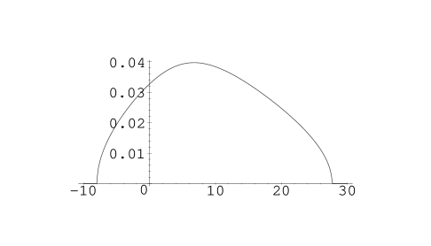
Figure 1: The eigenvalue distribution $\rho_{A}({\tilde{\lambda}})$. Equivalently, the density of stretched string states vs. (mass)² for a probe at the center of a Gaussian ensemble.

The distribution of eigenvalues of the matrix $B$ can be obtained starting from the Wigner semicircle (25). It is given by

$$\rho_{B}({\tilde{\lambda}})={1\over 8\pi{\tilde{b}}^{2}}\sqrt{16{\tilde{b}}^{2}-\left({\tilde{\lambda}}-{\tilde{b}}^{2}\right)^{2}}$$

where the dimensionless probe position ${\tilde{b}}$ is defined by ${\tilde{b}}=|b|/\sigma_{\rm eff}$. Note that the eigenvalues of $B$ lie in the interval

$${\tilde{b}}^{2}-4{\tilde{b}}\,\leq\,{\tilde{\lambda}}_{B}\,\leq\,{\tilde{b}}^{2}+4{\tilde{b}}\,.$$ (29)

Having found the spectra of $A$ and $B$ separately, the lowest eigenvalue of $M^{2}=A+B$ can be bounded by

$$\lambda_{A}^{\rm min}+\lambda_{B}^{\rm min}\,\leq\,\lambda_{M^{2}}^{\rm min}\,\leq\,\lambda_{A}^{\rm min}+\lambda_{B}^{\rm max}\,.$$ (30)

If $b=0$, so the probe is located at the origin, then the matrix $B$ vanishes, and the eigenvalue distribution of $M^{2}$ is given in Fig. 1: a probe 0-brane placed at the center of a Gaussian ensemble has many tachyonic modes. As $|b|$ increases the eigenvalues of $M^{2}$ tend to increase, and eventually a critical radius is reached at which there are no more tachyons. Applying the inequality (30) to the results (28), (29) we can say that the smallest eigenvalue of $M^{2}$ lies in the range

$${\tilde{b}}^{2}-4{\tilde{b}}-8.0\,\leq\,{\tilde{\lambda}}_{M^{2}}^{\rm min}\,\leq\,{\tilde{b}}^{2}+4{\tilde{b}}-8.0\,.$$ (31)

It then follows that the critical tachyon radius, at which the smallest eigenvalue of $M^{2}$ vanishes, lies somewhere in the interval $1.47<{\tilde{b}}_{\rm crit}<5.47$. Restoring units, this reads

$$1.47\sigma_{\rm eff}<|b|_{\rm crit}<5.47\sigma_{\rm eff}\,.$$

Recall from (26) that the largest eigenvalue of the matrices ${\bf X}_{i}$ is $2\sigma_{\rm eff}$. So we see that the tachyon instability sets in at roughly the same radius as the size of the object defined by its range of eigenvalues.

5 Conclusions

We have argued that the horizon of a Schwarzschild black hole (or more precisely, a trapped surface) is seen by a 0-brane probe in M(atrix) theory as a critical radius at which a tachyon develops. This gives an interesting picture of the process by which such a black hole is formed. One starts with a collection of 0-branes located far from each other. With the right initial momenta they will approach each other and some string creation will take place. If enough strings are created then a tachyon region will form. If the size of the tachyon region is $\gg l_{p}$ then a macroscopic black hole has been created. If another 0-brane approaches the black hole, it will be absorbed when it enters the tachyon region. In the absorption process the tachyon rolls down its potential and, via its couplings to the other 0-branes making up the black hole, thermalizes the infalling matter.

Since we do not have good control over the wavefunction of a Schwarzschild black hole, we cannot conclusively show that it has a tachyon region. But by analyzing some examples where a tachyon instability arises in M(atrix) theory, we showed that the TIR has reasonable properties to be an indicator for a Schwarzschild horizon. We gave examples which have macroscopic tachyon regions, even in the large $N$ limit. We also studied membrane states, where the TIR vanishes at large $N$.

The most interesting example we analyzed was the tachyon instability for Gaussian random matrices. In this large-$N$ calculation we showed that the size of the tachyon region is roughly the same as the spread of 0-brane positions. It is conceivable that the Gaussian ensemble is a good variational approximation to the true wavefunction of a Schwarzschild black hole at the BFKS point. At least in the non-supersymmetric case, Gaussians have been shown to give a fairly good approximation for large-$N$ Yang-Mills quantum mechanics [32]. The crucial test of this idea is to include the fermions and compute the mass of a typical state in the Gaussian ensemble [31].

We expect that much of our discussion of tachyon instabilities can be carried over to other non-extremal black holes built out of D-branes. And given the conjectured relation between finite temperature SYM and black holes in AdS space [14], our proposal suggests that the phenomenon of tachyon instability can also be used as a gauge theory indicator for the horizon of a non-extremal AdS black hole.

Acknowledgements

We are grateful to Constantin Bachas, Misha Fogler, Anton Kapustin, Igor Klebanov, Samir Mathur, Steve Shenker, and Lenny Susskind for valuable discussions. The work of DK is supported in part by the Department of Energy under contract DE-FG02-90ER40542 and by a Hansmann Fellowship. The work of GL is supported by the NSF under grant PHY-91-57482.

Appendix A Gaussian Random Matrices

In this appendix we review some techniques of random matrix theory, and derive the cubic equation (27) satisfied by the resolvent ${\cal R}_{A}$.

The standard reference on random matrix theory is the book by Mehta [33]. The methods we will use were explained to us by Misha Fogler. Although we are not sure of original references similar methods appear in the literature in [34].

To introduce the method, we start by considering a single $N\times N$ Hermitian matrix ${\bf X}$ chosen at random from the probability distribution

$$P({\bf X})={\rm const.}\,\,\,\exp\left(-{1\over 2\sigma^{2}}{\rm Tr}({\bf X}^{2})\right)\,.$$

We are interested in finding the ensemble average of the Green’s function

$$G(\lambda)={1\over\lambda-{\bf X}}\,.$$

$G(\lambda)$ can be expanded in perturbation theory, in terms of a ‘propagator’ $G_{0}={1\over\lambda}{\hbox to0.0pt{1\hss}\hskip 1.6pt\hbox{1}}$ and an ‘interaction’ ${\bf X}$, as

$$G=G_{0}+G_{0}{\bf X}G_{0}+G_{0}{\bf X}G_{0}{\bf X}G_{0}+\cdots\,.$$

To compute $<G>$ we must contract the ${\bf X}$ matrices in all possible ways using the two-point function

$$<{\bf X}_{ab}{\bf X}_{cd}>=\sigma^{2}\delta_{ad}\delta_{bc}\,.$$

We take the large $N$ limit holding the ’t Hooft coupling $\sigma^{2}_{\rm eff}=N\sigma^{2}$ fixed. Then the diagrams which contribute to $<G>$ at leading order in $1/N$ are the rainbow diagrams, in which ${\bf X}$ propagators do not cross. The same set of diagrams appear in the solution of large-$N$ QCD in 1+1 dimensions [35]. They can be summed by setting

$$<G>=G_{0}+G_{0}\Sigma<G>$$

where the amputated, 1PI (with respect to $G_{0}$) self-energy satisfies

$$\Sigma = \kern 6.0pt\mathop{\vbox{\halign{#\cr\kern 3.0pt\cr$\braceld\leaders\vrule height=0.39998pt,depth=0.0pt\hfill\bracerd$\crcr\kern 5.0pt\nointerlineskip\cr$\hfil\displaystyle{\kern-6.0pt{\bf X}<G>{\bf X}\kern-6.0pt}\hfil$\crcr}}}\kern 6.0pt$$

$$= \sigma^{2}{\hbox to0.0pt{1\hss}\hskip 1.6pt\hbox{1}}_{N\times N}\,{\rm Tr}<G>$$

Combining these two equations yields a quadratic equation satisfied by the resolvent ${\cal R}\equiv{\sigma_{\rm eff}\over N}{\rm Tr}<G>$. Working in terms of the dimensionless quantity ${\tilde{\lambda}}=\lambda/\sigma_{\rm eff}$ the resolvent satisfies

$${\cal R}^{2}-{\tilde{\lambda}}{\cal R}+1=0\,.$$

Taking the appropriate solution to this equation, one finds that ${\cal R}({\tilde{\lambda}})$ has a negative imaginary part for $-2\leq{\tilde{\lambda}}\leq 2$, and that the distribution of eigenvalues of ${\bf X}$ is

$$\rho({\tilde{\lambda}})=-{1\over\pi}{\rm Im}\,{\cal R}({\tilde{\lambda}}+i\epsilon)={1\over 2\pi}\sqrt{4-{\tilde{\lambda}}^{2}}\,.$$

This is Wigner’s semicircle distribution (25), written in terms of ${\tilde{\lambda}}$.

Next we consider a slightly more involved example, which has many of the features of the full problem. Let ${\bf X}$ and ${\bf Y}$ be two independent Hermitian matrices chosen at random from identical Gaussian distributions. To determine the eigenvalues of the commutator $i[{\bf X},{\bf Y}]$ we introduce as before

$$G(\lambda) = {1\over\lambda-i[{\bf X},{\bf Y}]}$$

$$<G> = G_{0}+G_{0}\Sigma<G>$$

The 1PI self-energy is given by

$$\Sigma = \kern 6.0pt\mathop{\vbox{\halign{#\cr\kern 3.0pt\cr$\braceld\leaders\vrule height=0.39998pt,depth=0.0pt\hfill\bracerd$\crcr\kern 5.0pt\nointerlineskip\cr$\hfil\displaystyle{\kern-6.0pt{\bf X}<{\bf Y}G{\bf Y}>{\bf X}\kern-6.0pt}\hfil$\crcr}}}\kern 6.0pt+\kern 6.0pt\mathop{\vbox{\halign{#\cr\kern 3.0pt\cr$\braceld\leaders\vrule height=0.39998pt,depth=0.0pt\hfill\bracerd$\crcr\kern 5.0pt\nointerlineskip\cr$\hfil\displaystyle{\kern-6.0pt{\bf Y}<{\bf X}G{\bf X}>{\bf Y}\kern-6.0pt}\hfil$\crcr}}}\kern 6.0pt$$

$$= \sigma^{2}{\hbox to0.0pt{1\hss}\hskip 1.6pt\hbox{1}}_{N\times N}{\rm Tr}<{\bf X}G{\bf X}>+\sigma^{2}{\hbox to0.0pt{1\hss}\hskip 1.6pt\hbox{1}}_{N\times N}{\rm Tr}<{\bf Y}G{\bf Y}>$$

The quantities appearing on the right hand side in turn satisfy

$$<{\bf X}G{\bf X}> = \kern 6.0pt\mathop{\vbox{\halign{#\cr\kern 3.0pt\cr$\braceld\leaders\vrule height=0.39998pt,depth=0.0pt\hfill\bracerd$\crcr\kern 5.0pt\nointerlineskip\cr$\hfil\displaystyle{\kern-6.0pt{\bf X}<G>{\bf X}\kern-6.0pt}\hfil$\crcr}}}\kern 6.0pt+\kern 6.0pt\mathop{\vbox{\halign{#\cr\kern 3.0pt\cr$\braceld\leaders\vrule height=0.39998pt,depth=0.0pt\hfill\bracerd$\crcr\kern 5.0pt\nointerlineskip\cr$\hfil\displaystyle{\kern-6.0pt{\bf X}<G>{\bf X}\kern-6.0pt}\hfil$\crcr}}}\kern 6.0pt<{\bf Y}G{\bf Y}>\kern 6.0pt\mathop{\vbox{\halign{#\cr\kern 3.0pt\cr$\braceld\leaders\vrule height=0.39998pt,depth=0.0pt\hfill\bracerd$\crcr\kern 5.0pt\nointerlineskip\cr$\hfil\displaystyle{\kern-6.0pt{\bf X}<G>{\bf X}\kern-6.0pt}\hfil$\crcr}}}\kern 6.0pt$$

$$= \sigma^{2}{\hbox to0.0pt{1\hss}\hskip 1.6pt\hbox{1}}_{N\times N}{\rm Tr}<G>+\sigma^{4}<{\bf Y}G{\bf Y}>\left({\rm Tr}<G>\right)^{2}$$

$$<{\bf Y}G{\bf Y}> = \kern 6.0pt\mathop{\vbox{\halign{#\cr\kern 3.0pt\cr$\braceld\leaders\vrule height=0.39998pt,depth=0.0pt\hfill\bracerd$\crcr\kern 5.0pt\nointerlineskip\cr$\hfil\displaystyle{\kern-6.0pt{\bf Y}<G>{\bf Y}\kern-6.0pt}\hfil$\crcr}}}\kern 6.0pt+\kern 6.0pt\mathop{\vbox{\halign{#\cr\kern 3.0pt\cr$\braceld\leaders\vrule height=0.39998pt,depth=0.0pt\hfill\bracerd$\crcr\kern 5.0pt\nointerlineskip\cr$\hfil\displaystyle{\kern-6.0pt{\bf Y}<G>{\bf Y}\kern-6.0pt}\hfil$\crcr}}}\kern 6.0pt<{\bf X}G{\bf X}>\kern 6.0pt\mathop{\vbox{\halign{#\cr\kern 3.0pt\cr$\braceld\leaders\vrule height=0.39998pt,depth=0.0pt\hfill\bracerd$\crcr\kern 5.0pt\nointerlineskip\cr$\hfil\displaystyle{\kern-6.0pt{\bf Y}<G>{\bf Y}\kern-6.0pt}\hfil$\crcr}}}\kern 6.0pt$$

$$= \sigma^{2}{\hbox to0.0pt{1\hss}\hskip 1.6pt\hbox{1}}_{N\times N}{\rm Tr}<G>+\sigma^{4}<{\bf X}G{\bf X}>\left({\rm Tr}<G>\right)^{2}$$

Other terms which could appear on the right hand side either vanish identically or are subleading in $1/N$. This system of equations can be combined into a single cubic equation for ${\cal R}={\sigma^{2}_{\rm eff}\over N}{\rm Tr}<G>$. In terms of ${\tilde{\lambda}}\equiv\lambda/\sigma^{2}_{\rm eff}$, it reads

$${\tilde{\lambda}}{\cal R}^{3}+{\cal R}^{2}-{\tilde{\lambda}}{\cal R}+1=0\,.$$

Choosing the appropriate solution to this equation, one finds that the eigenvalue distribution of $i[{\bf X},{\bf Y}]$ is symmetric about zero, and is non-vanishing only for ${\tilde{\lambda}}$ between $\pm{1\over 2}\sqrt{22+10\sqrt{5}}$.

Finally, we turn to the spectrum of the matrix

$$A_{ij}=\delta_{ij}\sum_{k}{\bf X}_{k}^{2}+2[{\bf X}_{i},{\bf X}_{j}]$$

where the ${\bf X}_{i}$ are independent, identically distributed $N\times N$ Gaussian random matrices. We let $i,j=1,\ldots,d$ so that $A$ is an $Nd\times Nd$ matrix. As above we set

$$G(\lambda) = {1\over\lambda-A}$$

$$<G> = G_{0}+G_{0}\Sigma<G>$$

where now $G_{0}={1\over\lambda}{\hbox to0.0pt{1\hss}\hskip 1.6pt\hbox{1}}_{Nd\times Nd}$. The self-energy is given by

$$\Sigma_{ij}=\kern 6.0pt\mathop{\vbox{\halign{#\cr\kern 3.0pt\cr$\braceld\leaders\vrule height=0.39998pt,depth=0.0pt\hfill\bracerd$\crcr\kern 5.0pt\nointerlineskip\cr$\hfil\displaystyle{\kern-6.0pt{\bf X}_{k}{\bf X}\kern-6.0pt}\hfil$\crcr}}}\kern 6.0pt{}_{k}\delta_{ij}+<\kern 6.0pt\mathop{\vbox{\halign{#\cr\kern 3.0pt\cr$\braceld\leaders\vrule height=0.39998pt,depth=0.0pt\hfill\bracerd$\crcr\kern 5.0pt\nointerlineskip\cr$\hfil\displaystyle{\kern-6.0ptA_{ik}G_{kl}A\kern-6.0pt}\hfil$\crcr}}}\kern 6.0pt{}_{lj}>$$

where the contractions in the second term mean that the two outermost ${\bf X}_{i}$’s which appear in $A_{ik}$, $A_{lj}$ are to be contracted. This equation can be simplified somewhat by making use of $SO(d)$ invariance, which implies that we can set

$$G_{ij}={1\over d}\delta_{ij}G_{kk}\qquad\Sigma_{ij}={1\over d}\delta_{ij}\Sigma_{kk}\,.$$

Then one has

$$\Sigma_{ij} = \kern 6.0pt\mathop{\vbox{\halign{#\cr\kern 3.0pt\cr$\braceld\leaders\vrule height=0.39998pt,depth=0.0pt\hfill\bracerd$\crcr\kern 5.0pt\nointerlineskip\cr$\hfil\displaystyle{\kern-6.0pt{\bf X}_{k}{\bf X}\kern-6.0pt}\hfil$\crcr}}}\kern 6.0pt{}_{k}\delta_{ij}+{1\over d}<\kern 6.0pt\mathop{\vbox{\halign{#\cr\kern 3.0pt\cr$\braceld\leaders\vrule height=0.39998pt,depth=0.0pt\hfill\bracerd$\crcr\kern 5.0pt\nointerlineskip\cr$\hfil\displaystyle{\kern-6.0ptA_{ik}G_{ll}A\kern-6.0pt}\hfil$\crcr}}}\kern 6.0pt{}_{kj}>$$

$$= Nd\sigma^{2}\delta_{ij}{\hbox to0.0pt{1\hss}\hskip 1.6pt\hbox{1}}_{N\times N}+{9d-8\over d^{2}}\sigma^{2}\delta_{ij}{\hbox to0.0pt{1\hss}\hskip 1.6pt\hbox{1}}_{N\times N}{\rm Tr}<{\bf X}_{k}G_{ll}{\bf X}_{k}>\,.$$

The quantity appearing on the right hand side in turn satisfies

$$<{\bf X}_{k}G_{ll}{\bf X}_{k}> = \kern 6.0pt\mathop{\vbox{\halign{#\cr\kern 3.0pt\cr$\braceld\leaders\vrule height=0.39998pt,depth=0.0pt\hfill\bracerd$\crcr\kern 5.0pt\nointerlineskip\cr$\hfil\displaystyle{\kern-6.0pt{\bf X}_{k}<G_{ll}>{\bf X}\kern-6.0pt}\hfil$\crcr}}}\kern 6.0pt{}_{k}+\kern 6.0pt\mathop{\vbox{\halign{#\cr\kern 3.0pt\cr$\braceld\leaders\vrule height=0.39998pt,depth=0.0pt\hfill\bracerd$\crcr\kern 5.0pt\nointerlineskip\cr$\hfil\displaystyle{\kern-6.0pt{\bf X}_{k}<G_{lm}>A\kern-6.0pt}\hfil$\crcr}}}\kern 6.0pt\kern-5.0pt\kern 6.0pt\mathop{\vbox{\halign{#\cr\kern 3.0pt\cr$\braceld\leaders\vrule height=0.39998pt,depth=0.0pt\hfill\bracerd$\crcr\kern 5.0pt\nointerlineskip\cr$\hfil\displaystyle{\kern-6.0pt\kern 5.0pt{}_{mn}<G_{nl}>{\bf X}\kern-6.0pt}\hfil$\crcr}}}\kern 6.0pt{}_{k}$$

$$+\kern 6.0pt\mathop{\vbox{\halign{#\cr\kern 3.0pt\cr$\braceld\leaders\vrule height=0.39998pt,depth=0.0pt\hfill\bracerd$\crcr\kern 5.0pt\nointerlineskip\cr$\hfil\displaystyle{\kern-6.0pt{\bf X}_{k}<G_{lm}><A\kern-6.0pt}\hfil$\crcr}}}\kern 6.0pt{}_{mn}G_{no}\kern 6.0pt\mathop{\vbox{\halign{#\cr\kern 3.0pt\cr$\braceld\leaders\vrule height=0.39998pt,depth=0.0pt\hfill\bracerd$\crcr\kern 5.0pt\nointerlineskip\cr$\hfil\displaystyle{\kern-6.0ptA_{op}><G_{pl}>{\bf X}\kern-6.0pt}\hfil$\crcr}}}\kern 6.0pt{}_{k}$$

$$= d\sigma^{2}{\hbox to0.0pt{1\hss}\hskip 1.6pt\hbox{1}}_{N\times N}{\rm Tr}<G_{kk}>+\sigma^{4}{\hbox to0.0pt{1\hss}\hskip 1.6pt\hbox{1}}_{N\times N}\left({\rm Tr}<G_{kk}>\right)^{2}$$

$$+{9d-8\over d^{3}}\sigma^{4}<{\bf X}_{k}G_{ll}{\bf X}_{k}>\left({\rm Tr}<G_{mm}>\right)^{2}$$

There is a unique choice of contractions which contribute at leading order in $1/N$, since the ${\bf X}$ propagators cannot cross and the expectation value of an odd number of ${\bf X}_{i}$’s vanishes. The second equality is most easily obtained with the help of $SO(d)$ invariance.

This set of equations can be combined into a single cubic equation satisfied by the resolvent ${\cal R}_{A}={\sigma^{2}_{\rm eff}\over Nd}{\rm Tr}<G>$. In terms of $\tilde{\lambda}={\lambda\over\sigma^{2}_{\rm eff}}$ the equation reads

$$(9d-8){\tilde{\lambda}}{\cal R}_{A}^{3}+(9d-8)(d-1){\cal R}_{A}^{2}+d(d-{\tilde{\lambda}}){\cal R}_{A}+d=0\,.$$

Setting $d=9$, this is the result (27) given in the text.

References

- [1] T. Banks, W. Fischler, S. Shenker, and L. Susskind, M Theory As A Matrix Model: A Conjecture, hep-th/9610043.
- [2] T. Banks, W. Fischler, I. R. Klebanov, and L. Susskind, Schwarzschild Black Holes from Matrix Theory, hep-th/9709091.
- [3] I. R. Klebanov and L. Susskind, Schwarzschild Black Holes in Various Dimensions from Matrix Theory, hep-th/9709108.
- [4] E. Halyo, Six Dimensional Schwarzschild Black Holes in M(atrix) Theory, hep-th/9709225.
- [5] G. Horowitz and E. Martinec, Comments on Black Holes in Matrix Theory, hep-th/9710217.
- [6] M. Li, Matrix Schwarzschild Black Holes in Large N limit, hep-th/9710226.
- [7] S. Das, S. Mathur, S. Rama, and P. Ramadevi, Boosts, Schwarzschild Black Holes and Absorption cross-sections in M theory, hep-th/9711003.
- [8] T. Banks, W. Fischler, I. Klebanov, and L. Susskind, Schwarzschild Black Holes in Matrix Theory II, hep-th/9711005.
- [9] H. Liu and A.A. Tseytlin, Statistical mechanics of D0-branes and Black hole thermodynamics, hep-th/9712063.
- [10] T. Banks, W. Fischler, and I. Klebanov, Evaporation of Schwarzschild Black Holes in Matrix Theory, hep-th/9712236.
- [11] N. Ohta and J.-G. Zhou, Euclidean Path Integral, D0-Branes and Schwarzschild Black Holes in Matrix Theory, hep-th/9801023.
- [12] M. Li and E. Martinec, Probing Matrix Black Holes, hep-th/9801070.
- [13] D. Lowe, Statistical Origin of Black Hole Entropy, hep-th/9802173.
-
[14]
J. Maldacena, The Large N Limit of Superconformal field theories
and supergravity, hep-th/9711200;
N. Itzhaki, J. Maldacena, J. Sonnenschein, and S. Yankielowicz, Supergravity and the Large Limit of Theories With Sixteen Supercharges, hep-th/9802042. - [15] C. Bachas and M. Porrati, Phys. Lett. B296 (1992) 77.
- [16] C. Bachas, D-brane dynamics, Phys. Lett. B374 (1996) 37, hep-th/9511043.
- [17] M. Douglas, D. Kabat, P. Pouliot, and S. Shenker, D-branes and Short Distances in String Theory, hep-th/9608024.
- [18] T. Banks and L. Susskind, Brane-Antibrane Forces, hep-th/9511194.
- [19] E. Gava, K. Narain, and M. Sarmadi, On the Bound States of and -Branes, hep-th/9704006.
- [20] A. Sen, Tachyon Condensation on the Brane Antibrane System, hep-th/9805170.
- [21] M. Douglas, J. Polchinski, and A. Strominger, Probing Five-Dimensional Black Holes with D-Branes, hep-th/9703031.
- [22] J. Maldacena, Probing near extremal black holes with D-branes, hep-th/9705053v3. See section 3 of the revised version.
- [23] M. Claudson and M. Halpern, Supersymmetric Ground State Wavefunctions, Nucl. Phys. B250 (1985) 689.
- [24] See I. Gradshteyn and I. Ryzhik, Table of Integrals, Series, and Products, 4th ed. (Academic Press, 1980), section on norms.
-
[25]
J. Goldstone, unpublished; J. Hoppe, MIT Ph.D. thesis
(1982);
J. Hoppe, in Proc. Int. Workshop on Constraint’s Theory and Relativistic Dynamics, G. Longhi and L. Lusanna, eds. (World Scientific, 1987). - [26] B. de Wit, J. Hoppe and H. Nicolai, Nucl. Phys. B305 [FS 23] (1988) 545.
- [27] D. Kabat and W. Taylor, Spherical Membranes in M(atrix) Theory, hep-th/9711078.
- [28] S.-J. Rey, Gravitating M(atrix) Q-Balls, hep-th/9711081.
- [29] O. Aharony and M. Berkooz, Membrane Dynamics in M(atrix) Theory, hep-th/9611215.
- [30] G. Lifschytz and S. Mathur, Supersymmetry and Membrane Interactions in M(atrix) Theory, hep-th/9612087.
- [31] D. Kabat and G. Lifschytz, in preparation.
- [32] M. Engelhardt and S. Levit, Variational Master Field for Large- Interacting Matrix Models – Free Random Variables on Trial, hep-th/9609216.
- [33] M. L. Mehta, Random Matrices, 2nd ed. (Academic Press, 1991).
-
[34]
A. Pandey, Ann. Phys. 134, 110 (1981);
T. A. Brody, J. Flores, J. B. French, P. A. Mello, A. Pandey, and S. S. M. Wong, Rev. Mod. Phys. 53, 385 (1981);
E. Brezin and A. Zee, Phys. Rev. E49, 2588 (1994). -
[35]
G. ’t Hooft, Nucl. Phys. B75 (1974) 461;
S. Coleman, Aspects of Symmetry (Cambridge, 1985), p. 378.