Non-Abelian Stokes Theorem for Loop Variables
Associated with Nontrivial Loops

Abstract

The non-abelian Stokes theorem for loop variables associated with nontrivial loops (knots and links) is derived. It is shown that a loop variable is in general different from unity even if the field strength vanishes everywhere on the surface surrounded by the loop.

1 Introduction

As is well known, the Stokes theorem is remarkable for its generality : the formula

$$\int_{\partial M}\omega=\int_{M}d\omega$$ (1)

is valid for any $(d+1)$-dimensional oriented manifold $M$ with the boundary $\partial M$, where $\omega$ is a $d$-form on $M$. It should be noted that $\omega$ and $M$ in $(1\cdot 1)$ can be replaced with a $p$-form and a $(p+1)$-chain with $p\leq d$, respectively. Its usefulness manifests in the following formula of electromagnetism :

$$\int_{\partial\sigma}a_{\mu}(x)dx^{\mu}=\frac{1}{2}\int\int_{\sigma}f_{\mu\nu}(x)dx^{\mu}\wedge dx^{\nu},$$ (2)

$$f_{\mu\nu}(x)=\partial_{\mu}a_{\nu}(x)-\partial_{\nu}a_{\mu}(x),$$ (3)

where $\sigma,a_{\mu}(x)$ and $f_{\mu\nu}(x)$ are a two-dimensional oriented surface in the spacetime, the electromagnetic potential and the electromagnetic field strength, respectively.
On the other hand, if we consider the non-Abelian gauge potential

$$A_{\mu}(x)=A^{a}_{\mu}(x)T^{a},\hskip 14.22636ptT^{a}:\mbox{\rm generator of the gauge group},$$ (4)

and the field strength

$$F_{\mu\nu}(x)=\partial_{\mu}A_{\nu}(x)-\partial_{\nu}A_{\mu}(x)-ig[A_{\mu}(x),A_{\nu}(x)],$$ (5)

with $g$ being the gauge coupling constant, we have $\int_{\partial\sigma}A_{\mu}(x)dx^{\mu}=\frac{1}{2}\int\int_{\sigma}\bigl{\{}\partial_{\mu}A_{\nu}(x)-\partial_{\nu}A_{\mu}(x)\bigl{\}}dx^{\mu}\wedge dx^{\nu}\neq\frac{1}{2}\int\int_{\sigma}F_{\mu\nu}(x)dx^{\mu}\wedge dx^{\nu}.$ We see that a line integral of the gauge potential cannot be converted to a surface integral of the field strength in non-Aberian gauge theory.

An important variable of the non-Abelian gauge field theory is the loop variable $(\gamma)$ defined by[1]rf:5

$$\left.\begin{array}[]{l}(\gamma)=P_{\kappa}e^{ig\int_{0}^{1}d\kappa A_{\mu}(x(\kappa))\frac{dx^{\mu}(\kappa)}{d\kappa}},\\ \\ P_{\kappa}:\hskip 8.53581pt\kappa\mbox{\rm-ordering},\\ \end{array}\right.$$ (6)

where the loop $\gamma$ is parametrized by the parameter $\kappa$ as $\gamma=\{x(\kappa)|0\leq\kappa\leq 1\}$. Under the gauge transformation

$$A_{\mu}(x)\rightarrow{A^{{}^{\prime}}}_{\mu}(x)=h(x)A_{\mu}(x)h^{-1}(x)+\frac{i}{g}h(x)\partial_{\mu}h^{-1}(x),$$ (7)

the loop variable $(\gamma)$ transforms as

$$(\gamma)\rightarrow h(x(0))(\gamma)h^{-1}(x(0)),$$ (8)

where the point $x(0)$ is the starting point of $\gamma$, which should coincide with the end point $x(1)$. When the loop $\gamma$ is trivial,i.e., unknotted and unlinked, the loop variable $(\gamma)$ is equal to the following quantity :

$$[S]\equiv P_{t}e^{ig\int_{0}^{1}dt\int_{0}^{1}ds{\mathcal{F}_{\mu\nu}}(x(s,t))\frac{\partial x^{\mu}(s,t)}{\partial s}\frac{\partial x^{\nu}(s,t)}{\partial t}},$$

$${\mathcal{F}_{\mu\nu}}(x)=w(x)F_{\mu\nu}(x)w^{-1}(x),$$ (9)

$$P_{t}\hskip 8.53581pt:\hskip 14.22636ptt\mbox{\rm-ordering},$$

where $w(x)$ is a unitary matrix depending on a path from $x(0,0)$ to $x(s,t)$ and the boundary $\partial S$ of the simply connected surface $S=\{x(s,t)|(s,t)\in\Sigma\}$, $\Sigma=\{(s,t)|0\leq s,t\leq 1\}$, is assumed to be equal to the loop $\gamma$. The $x(0)=x(1)$ in (1$\cdot$6) sould coincide with the $x(0,0)$ in (1$\cdot$9). The equality

$$(\gamma)=[S],\hskip 14.22636pt\gamma=\partial S$$ (10)

is called the non-Abelian Stokes theorem(NAST).[6]rf:15 For a given loop $\gamma$, there exist many surfaces satisfying $\partial S=\gamma$, which are continuously deformable to each other. It was shown that the Bianchi identity

$$\left.\begin{array}[]{l}[D_{\rho},F_{\mu\nu}]+[D_{\mu},F_{\nu\rho}]+[D_{\nu},F_{\rho\mu}]=0,\\ \\ D_{\rho}=\partial_{\rho}-igA_{\rho},\\ \end{array}\right.$$ (11)

guarantees the invariance of $[S]$ under continuous deformations of $S$.[15] In other words, for the variation

$$x(s,t)\rightarrow x(s,t)+\delta x(s,t),$$ (12)

with the property

$$\delta x(s,t)=0,\hskip 5.69054pt(s,t)\in\partial\Sigma,$$ (13)

we have

$$\delta[S]=0.$$ (14)

In the above, we have stated the NAST (1$\cdot$10) under the assumption that the loop $\gamma$ is trivial and surrounds the simply connected surface $S$. If the loop $\gamma$ is nontrivial and the surface $S$ is not simply connected, the parameter space $\Sigma$ must be chosen more complicated than the above $\{(s,t)|0\leq s,t\leq 1\}$. The purpose of the present paper is to explore how the NAST should be modified when the loop $\gamma$ is a knot or a link. We shall find that rather simple applications of the knot theory[16, 17] leads us to the NAST in such cases. We shall also find that the loop variable $(\gamma)$ can be different from unity even if the field strength $F_{\mu\nu}(x)$ vanishes at every point on the surface $S$.

This paper is organized as follows. In §2, we obtain the NAST for the case that the loop is a trefoil knot. After obtaining the NAST for a Hopf link in §3, we discuss the NAST for an arbitrary loop in §4. The final section, §5, is devoted to summary.

2 NAST for a trefoil knot

Before considering the general case, we discuss in the present and the next sections loop variables associated with some simple but nontrivial loops. Assuming that the loops$\subset$R${}^{3}\subset$spacetime, we begin with the case of a trefoil knot.

2.1 Surfaces surrounded by a trefoil knot

The first task to be done is to find an oriented surface whose boundary is ambient isotopic, i.e., continuously deformable in R³, to a trefoil knot shown in Fig.1. There exists a standerd method called the Seifert algorithm to construct surfaces with desired properties.

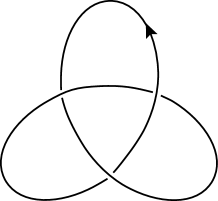
Figure 1: A trefoil knot.

It is not difficult to recognize that the surfaces $S$, $S^{\prime}$ and $S^{\prime\prime}$ in Fig.2 are three such examples.

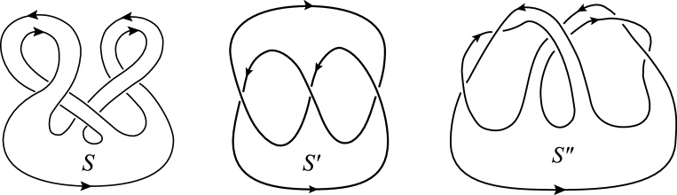
Figure 2: Seifert surfaces for loops ambient isotopic to a trefoil knot.

The surface $S$ is said to be of the Seifert standard form. It is clear that the surface $S$ is homeomorphic to the surface $\Sigma$ of Fig.3 : there exist a continuous bijection $x:\Sigma\rightarrow S$ and $x^{-1}$ : $S\rightarrow\Sigma$ is also continuous. As is explained in §4, a surface whose boundary coincides with a given link is called the Seifert surface of the link. surface $S$ is homeomorphic to the surface $\Sigma$ of Fig.3 : there exist a continuous bijection $x:\Sigma\rightarrow S$ and $x^{-1}$ : $S\rightarrow\Sigma$ is also continuous. As is explained in §4, a surface whose boundary coincides with a given link is called the Seifert surface of the link.

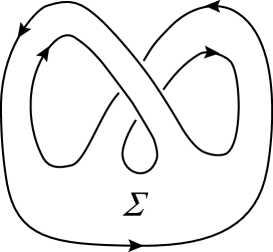
Figure 3: The parameter space for a Seifert surface of a trefoil knot.

We are allowed to regard the surface $S$ an oriented surface in the spacetime satisfying $\partial S=\gamma$ and assume $S=\{x(s,t)|(s,t)\in\Sigma\}$. Here the surface $\Sigma$ plays the role of the parameter space which was necessary in the description of the NAST in §1. Our procedure can be stated as follows. We first choose the parameter space $\Sigma$ to be of the allowed simplest structure. The surface $S$ embedded in the spacetime is given as $S=x(\Sigma)$, where the mapping $x$ may cause some twists and linkings of bands.

2.2 Decomposition of $\Sigma$ into simply connected surfaces

Although there are many ways to decompose the surface $\Sigma$ into some simply connected surfaces, we adopt the manner shown in Fig.4.

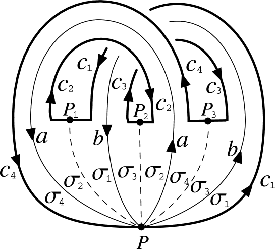
Figure 4: A decomposition of the parameter space into simply connected surfaces.

The surfaces $\sigma_{i},\hskip 2.84526pti=1,2,3,4$, in Fig.4 satisfying $\Sigma=\bigcup_{i=1}^{4}\sigma_{i}$ correspond to the surfaces $S_{i},i=1,2,3,4$, in the spacetime, respectively :

$$S=\bigcup_{i=1}^{4}S_{i},\hskip 5.69054ptS_{i}=x(\sigma_{i}).$$ (15)

Similarly the portions $c_{i}$, $i=1,2,3,4,$ of the boundary of $\Sigma$ correspond to those of the trefoil knot $\gamma$ in the spacetime :

$$\gamma=\gamma_{4}\circ\gamma_{3}\circ\gamma_{2}\circ\gamma_{1},\hskip 14.22636pt\gamma=x(c_{i}).$$ (16)

The points $P_{i-1}$ and $P_{i}$ denote the starting and the end points of $c_{i}$, $i=1,2,3,4,$ $P_{0}\equiv P_{4}\equiv P$,respectively. The curves $a$ and $b$ are two independent elements of the first homology group of $\Sigma$.We have thus decomposed the surface $\Sigma$ into four simply connected surfaces $\sigma_{i},\hskip 5.69054pti=1,2,3,4,$ with the help of $a,b,d_{1},d_{2}$ and $d_{3}$, where $d_{i}$ is a curve starting at $P_{i}$ and ending at $P$.

2.3 Derivation of NAST

The surface $\sigma_{1}$ is surrounded by the boundary $\overline{b}\circ d_{1}\circ c_{1}$, where $\overline{b}$ is $b$ with the orientation reversed. Since the surface $\sigma_{1}$ is simply connected, we can apply the NAST of §1 with $S=S_{1}=x(\sigma_{1})$ and $\gamma=\partial S_{1}=\overline{B}\circ D_{1}\circ\gamma_{1}=x(\overline{b}\circ d_{1}\circ c_{1})$, where $\overline{B}$ and $D_{i}$ are defined by

$$\overline{B}=x(\overline{b}),\hskip 14.22636ptD_{i}=x(d_{i}).$$ (17)

We then have

$$[S_{1}]=(\overline{B})(D_{1})(\gamma_{1}),$$ (18)

where $[*]$ and $(*)$ are defined in analogous manners to $(1\cdot 9)$ and $(1\cdot 6)$, respectively. From $(2\cdot 4)$, we obtain

$$(\gamma_{1})=(D_{1})^{-1}(B)[S_{1}],$$ (19)

where we have made use of the relation $(\overline{B})=(B)^{-1}$. Similarly we have

$$\left.\begin{array}[]{l}(A)(D_{2})(\gamma_{2})(\overline{D_{1}})=[S_{2}],\\ \\ (B)(D_{3})(\gamma_{3})(\overline{D_{2}})=[S_{3}],\\ \\ (\overline{A})(\gamma_{4})(\overline{D_{3}})=[S_{4}],\\ \end{array}\right.$$ (20)

yielding

$$\left.\begin{array}[]{l}(\gamma_{2})=(D_{2})^{-1}(A)^{-1}[S_{2}](D_{1}),\\ \\ (\gamma_{3})=(D_{3})^{-1}(B)^{-1}[S_{3}](D_{2}),\\ \\ (\gamma_{4})=(A)[S_{4}](D_{3}),\\ \end{array}\right.$$ (21)

with

$$A=x(a).$$ (22)

Recalling that the loop variable $(\gamma)$ is given by

$$(\gamma)=(\gamma_{4})(\gamma_{3})(\gamma_{2})(\gamma_{1}),$$ (23)

and that the trivial loops $a$ and $b$ surround simply connected domains $\sigma_{a}$ and $\sigma_{b}$, respectively $(\partial\sigma_{a}=a$, $\partial\sigma_{b}=b)$, we are led to

$$\left.\begin{array}[]{l}(\gamma)=[S_{a}][S_{4}][S_{b}]^{-1}[S_{3}][S_{a}]^{-1}[S_{2}][S_{b}][S_{1}],\\ \\ \hskip 17.07164pt\equiv[[S]]\\ \end{array}\right.$$ (24)

where $S_{a}$ and $S_{b}$ are given by

$$S_{a}=x(\sigma_{a}),\hskip 5.69054ptS_{b}=x(\sigma_{b}).$$ (25)

The l.h.s. of (2$\cdot$10) concerns a contour integral of the non-Abelian gauge potential $A_{\mu}(x)$, while the r.h.s of (2$\cdot$10) with surface integrals of field strength. Eq. (2$\cdot$10) should be regarded as the NAST in the case that the loop $\gamma$ is a trefoil knot.

Some comments are in order.
(a) It is possible to think of a surface $\widetilde{S}$ which satisfies $\partial\widetilde{S}=\gamma$ and is oriented but cannot be continuously deformed to the above considered $S$. As will be discussed in §4, it can be shown that $[[S]]$ equals $[[\widetilde{S}]]$.
(b) Although the r.h.s. of (2$\cdot$10) may seem to depend on the choice of closed curves $a$ and $b$ on $\Sigma$, it is not the case : the r.h.s. of (2$\cdot$10) does not vary under small deformations of $a$ and $b$. This fact can be understood through the observations

$$\left.\begin{array}[]{l}\delta_{a}\bigl{(}[S_{a}]^{-1}[S_{2}]\bigl{)}=\delta_{a}\bigl{(}(D_{2})(\gamma_{2})(D_{1})^{-1}\bigl{)}=0,\\ \\ \delta_{b}\bigl{(}[S_{b}][S_{1}]\bigl{)}=\delta_{b}\bigl{(}(D_{1})(\gamma_{1})\bigl{)}=0,\end{array}\right.$$ (26)

etc., where $\delta_{a}$ and $\delta_{b}$ imply small deformations of $a$ and $b$, respectively.
(c) Eq. (2$\cdot$10) can be rewritten as follows :

$$\left.\begin{array}[]{l}(\gamma)={}^{g_{4}}[S_{4}]\hskip 5.69054pt{}^{g_{3}}[S_{3}]\hskip 5.69054pt{}^{g_{2}}[S_{2}]\hskip 5.69054pt{}^{g_{1}}[S_{1}]\hskip 5.69054pt[\xi]\\ \\ \hskip 17.07164pt=[\xi]\hskip 5.69054pt{}^{h_{4}}[S_{4}]\hskip 5.69054pt{}^{h_{3}}[S_{3}]\hskip 5.69054pt{}^{h_{2}}[S_{2}]\hskip 5.69054pt{}^{h_{1}}[S_{1}],\\ \end{array}\right.$$ (27)

with

$$[\xi]=[S_{a}][S_{b}]^{-1}[S_{a}]^{-1}[S_{b}],$$ (28)

$$\left.\begin{array}[]{l}{}^{g_{i}}[S_{i}]=g_{i}[S]g_{i}^{-1},\hskip 8.53581pt{}^{h_{i}}[S_{i}]=h_{i}[S_{i}]h_{i}^{-1},\\ \\ g_{1}=[\xi],\hskip 8.53581ptg_{2}=[S_{a}][S_{b}]^{-1}[S_{a}]^{-1},\\ \\ g_{3}=[S_{a}][S_{b}]^{-1},\hskip 8.53581ptg_{4}=[S_{a}],\\ \\ h_{1}=1,\hskip 8.53581pth_{2}=[S_{b}]^{-1},\hskip 8.53581pth_{3}=[S_{b}]^{-1}[S_{a}],\\ \\ h_{4}=[S_{b}]^{-1}[S_{a}][S_{b}].\\ \end{array}\right.$$ (29)

(d)The parameter space of the type of Fig.3 can be used for loops other than the trefoil knot. For example, the figure eight knot shown in Fig.5(a) has the Seifert surface of Fig.5(b), which is homeomorphic to the $\Sigma$ of Fig.3.

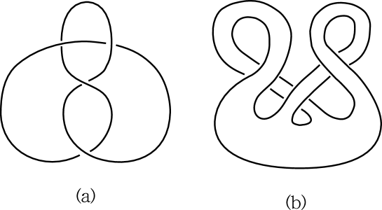
Figure 5: (a)A figure eight knot, (b)A Seifert surfaces of a loop ambient isotopic to a figure eight knot.

(e) In the Abelian case, Eq. $(2\cdot 10)$ reduces to $(\gamma)=[S_{4}][S_{3}][S_{2}][S_{1}]=[S]$.

2.4 Example

We consider the case that the loop $\gamma$ is the boundary of the surface $S^{\prime\prime\prime}$ shown in Fig.6, which is a deformed version of $S^{\prime\prime}$ of Fig.2.

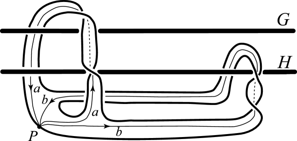
Figure 6: A deformed version of $S^{\prime\prime}$ of Fig.2.

We assume that $F_{\mu\nu}(x)$ does not vanish only in the neighbourhoods of the lines $G$ and $H$. Especially, we assume

$$F_{\mu\nu}(x)=0,\hskip 8.53581ptx\in S^{\prime\prime\prime}.$$ (30)

Then we have in general

$$[S_{a}]\neq 1,\hskip 8.53581pt[S_{b}]\neq 1,\hskip 8.53581pt\bigl{[}[S_{a}],[S_{b}]\bigl{]}\neq 0,$$ (31)

and

$$(\gamma)=[\xi]\neq 1.$$ (32)

We thus see that a round trip along a trefoil knot $\gamma$ can cause some physical effects even if $\gamma$ surrounds an area on which $F_{\mu\nu}(x)$ vanishes. To be more specific, we consider the case that the gauge group is $SU(2)$ and that the $T^{a}$ in (1$\cdot$4) belongs to the fundamental representation. Then we can assume

$$[S_{a}]=e^{\mbox{\it i{$A\cdot\sigma$}}},\hskip 8.53581pt[S_{b}]=e^{\mbox{\it i{$B\cdot\sigma$}}}$$ (33)

where $\sigma$$=(\sigma_{1},\sigma_{2},\sigma_{3})$ with $\sigma_{1},\sigma_{2},\sigma_{3}$ being Pauli matrices, and A and B are three dimensional real vectors. Defining K by

$$[\xi]=e^{\mbox{\it i{$K\cdot\sigma$}}},$$ (34)

the formula for the Wilson loop $W(\gamma)\equiv\mbox{\rm tr}(\gamma)$ is given by

$$W(\gamma)=2\cos K=2\bigl{[}1-2(\sin\varphi\sin\alpha\sin\beta)^{2}\bigl{]},$$ (35)

$$\alpha=|\mbox{\bf A}|,\hskip 8.53581pt\beta=|\mbox{\bf B}|,\hskip 8.53581pt\cos\varphi=\frac{\mbox{\bf A}\cdot\mbox{\bf B}}{\alpha\beta},\hskip 8.53581ptK=|\mbox{\bf K}|.$$ (36)

We have thus explicitly seen that the loop variable $(\gamma)$ and the Wilson loop $W(\gamma)$ are nontrivial if $\alpha$, $\beta$ as well as $\varphi$ are not equal to an integer multiple of $\pi$.

3 NAST for a Hopf link

We next investigate the NAST in the case that the loop $\gamma$ consists of some connected components. The simplest case is a Hopf link which consists of two connected components $\gamma_{1}$ and ${\gamma_{2}}^{\prime}$ as is shown in Fig.7(a) :

$$\gamma={\gamma_{2}}^{\prime}\circ\gamma_{1}.$$ (37)

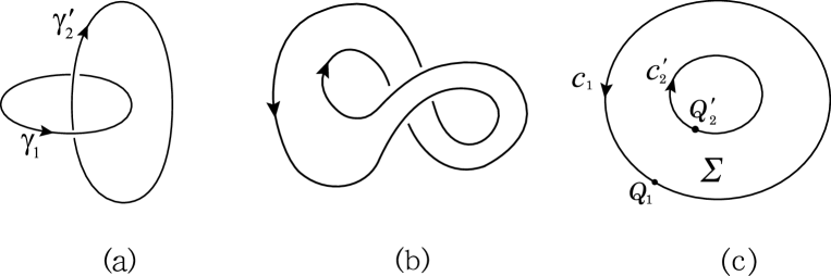
Figure 7: (a)A Hopf link, (b)A Seifert surfaces of a loop ambient isotopic to a Hopf link, (c)The parameter space for a Seifert surface of a Hopf link.

One of the Seifert surfaces of $\gamma$ is given in Fig.7(b), which is homeomorphic to the doubly connected surface $\Sigma$ of Fig.7(c) satisfying $\partial\Sigma={c_{2}}^{\prime}\circ c_{1}$. We are allowed to assume

$$\gamma_{1}=x(c_{1}),\hskip 8.53581pt{\gamma_{2}}^{\prime}=x({c_{2}}^{\prime}),$$ (38)

where $x$ is the mapping from $\Sigma$ to the spacetime. The simply connected surfaces $\sigma_{1}$ and ${\sigma_{2}}^{\prime}$ are surrounded by $c_{1}$ and $\overline{{c_{2}}^{\prime}}$, respectively. They are related to $\Sigma$ by

$$\Sigma=\sigma_{1}-{\sigma_{2}}^{\prime}.$$ (39)

If we set $S_{1}=x(\sigma_{1})$, ${S_{2}}^{\prime}=x({\sigma_{2}}^{\prime})$ and $S=x(\Sigma)$, we have

$$S=S_{1}-{S_{2}}^{\prime}.$$ (40)

Supposing that the loop $c_{1}({c_{2}}^{\prime})$ starts and ends at the point $Q_{1}({Q_{2}}^{\prime})$ and denoting a path from $Q_{1}$ to ${Q_{2}}^{\prime}$ by $d$, we define $D$ by $D=x(d)$. Now the NAST of §1 yields the following relations :

$$\left.\begin{array}[]{l}(\gamma_{1})=[S_{1}],\\ \\ (\overline{{\gamma_{2}}^{\prime}})=[{S_{2}}^{\prime}],\\ \\ (D)^{-1}({\gamma_{2}}^{\prime})(D)(\gamma_{1})=[S].\\ \end{array}\right.$$ (41)

We see that the NAST for the loop variable

$$(\gamma)=({\gamma_{2}}^{\prime})(\gamma_{1})$$ (42)

is given by

$$(\gamma)=\{S_{1};{S_{2}}^{\prime}\},$$ (43)

where $\{S_{1};{S_{2}}^{\prime}\}$ is defined by

$$\{S_{1};{S_{2}}^{\prime}\}=[{S_{2}}^{\prime}]^{-1}[S_{1}].$$ (44)

We see that the simple result $(\gamma)=[S]$, (1$\cdot$10), for a trivial loop is violated also in this example.

If we consider the case that the parameter space $\Sigma$ is $\mu$-ply connected as is shown in Fig.8, we are led to

$$(\gamma)=\{S_{1};{S_{2}}^{\prime},{S_{3}}^{\prime},\cdots{S_{\mu}}^{\prime}\}$$ (45)

where $(\gamma)$ and $\{S_{1};{S_{2}}^{\prime},{S_{3}}^{\prime},\cdots{S_{\mu}}^{\prime}\}$ are defined by

$$(\gamma)=({\gamma_{\mu}}^{\prime})\cdots({\gamma_{3}}^{\prime})({\gamma_{2}}^{\prime})(\gamma_{1}),$$ (46)

$$\{S_{1};{S_{2}}^{\prime},{S_{3}}^{\prime},\cdots{S_{\mu}}^{\prime}\}=[{S_{\mu}}^{\prime}]^{-1}\cdots[{S_{3}}^{\prime}]^{-1}[{S_{2}}^{\prime}]^{-1}[S_{1}].$$ (47)

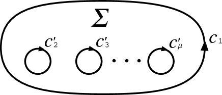
Figure 8: The parameter space of a link with $\mu$ connected components.

4 NAST for general links

In §2 and §3, we have considered the case of the simplest but nontrivial examples of knots and links. In this section we shall obtain the NAST for a loop variable associated with a general link.

4.1 Preliminaries[16, 17]

Let us consider a compact orientable surface $F$ and a link $L$ in $\mbox{\bf R}^{3}$. We say that $F$ is a Seifert surface of $L$ if the boundary of $F$ is equal to $L$ : $\partial F=L$. When a Seifert surface consists of some connected components, we can make a connected Seifert surface by the procedure of the connected sum which does not violate the relation $\partial F=L$. So, if necessary, we can assume that the Seifert surface is connected. The following theorem was discovered more than sixty years ago .
Theorem A. Any oriented link has a Seifert surface.

If $F$ is a Seifert surface of a link $L$, the surface $F^{\prime}$ obtained by the following procedure is also a Seifert surface of $L$ :

$$F^{\prime}=(F-E_{0}-E_{1})\cup h(S^{1}\times[0,1]),$$ (48)

where $E_{0}$ and $E_{1}$ are two disks inside $F$ satisfying $E_{0}\cap E_{1}=\phi$ and $h(S^{1}\times[0,1])$ is a handle to be attached to the surface $F-E_{0}-E_{1}$ along $\partial E_{0}=h(S^{1}\times\{0\})$ and $\partial E_{1}=h(S^{1}\times\{1\})$. If the handle $h(S^{1}\times[0,1])$ is attached on one side of $F-E_{0}-E_{1}$, the orientation of $F^{\prime}$ is naturally induced from that of $F$. For the above $F$ and $F^{\prime}$, we say that $F^{\prime}$ is obtained from $F$ by a 1-surgery. Conversely we say that $F$ is obtained from $F$ by a 0-surgery. The genus of a connected orientable surface $F$ is given by

$$g(F)=\frac{1}{2}\bigl{(}2-\chi(F)-\mu\bigl{)},$$ (49)

where $\mu$ is the number of the boundary components of $F$ and $\chi(F)$ is the Euler characteristic of $F$. We easily see

$$g(F^{\prime})=g(F)+1.$$ (50)

We then understand that, for a prescribed link, there are many Seifert surfaces with various values of genus. Among them a surface with the smallest genus is called the minimum Seifert surface. If two surfaces $F$ and $F^{\prime}$ are obtained by some steps of 0-and/or 1-surgeries from each other, they are said to be stably equivalent to each other. It can be seen that a 1-surgery of the surface $F$ is equivalent to attaching the closed surface $\overline{E_{0}}\cup h(S^{1}\times[0,1])\cup\overline{E_{1}}$ to $F$, where $\overline{E}$ is equal to $E$ with the orientation reversed. We have

$$[\overline{E_{0}}\cup h(S^{1}\times[0,1])\cup\overline{E_{1}}]=1$$ (51)

since the surface $\overline{E_{0}}\cup h(S^{1}\times[0,1])\cup\overline{E_{1}}$ is homeomorphic to a sphere and we know [sphere]=1. Furthermore there exists the following remarkable theorem.
Theorem B. Any two connected Seifert surfaces of an oriented link are stably equivalent to each other.

The genus $g(L)$ of a link $L$ is defined by $g(L)=g(F)$, where $g(F)$ is the genus of the minimum Seifert surface $F$ of $L$. As was stated in the above, we can assume that $F$ is connected. We here cite the classification theorem of surfaces.
Theorem C. Any connected orientable surface with boundaries is homeomorphic to one of $T(g,\mu)$, $g=0,1,2,\cdots,$ $\mu=1,2,3,\cdots,$ where $T(g,\mu)$ is given in Fig.9.

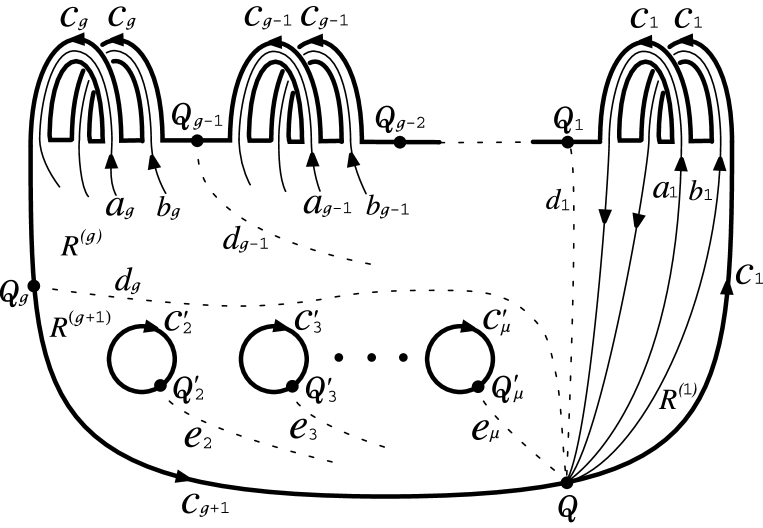
Figure 9: $T(g,\mu)$.

We note that $T(0,1)$ is a disk and that $T(1,1)$ and $T(0,\mu)$, $\mu\geq 2$, are given by Fig.3 and Fig.8, respectively.

4.2 Derivation of NAST for a general link

Suppose that a link $\gamma$ with the genus $g$ consists of $\mu$ connected components. We adopt one of the minimum Seifert surface of $\gamma$ and denote it by $S$. Then the surface $S$ can be expressed as

$$S=\{x(s,t)|(s,t)\in\Sigma\},\hskip 8.53581pt\Sigma=T(g,\mu),$$ (52)

where $x$ is, as in the previous sections, a continuous mapping from the parameter space $\Sigma$ to the spacetime. The curves $a_{i}$, $b_{i}$, $i=1,2,\cdots,g,$ and $e_{\alpha}$, $\alpha=2,3,\cdots,\mu$, in Fig.9 are helpful for the discussion of the loop variable $(\gamma)$. We assume that the link $\gamma$ is ordered as

$$\left.\begin{array}[]{l}\gamma=x(\partial\Sigma)\\ \\ \hskip 8.53581pt={\gamma_{\mu}}^{\prime}\circ{\gamma_{\mu-1}}^{\prime}\circ\cdots\circ{\gamma_{3}}^{\prime}\circ{\gamma_{2}}^{\prime}\circ\gamma_{g+1}\circ\gamma_{g}\circ\cdots\circ\gamma_{2}\circ\gamma_{1}\\ \end{array}\right.$$ (53)

with $\gamma_{i}$ and ${\gamma_{\alpha}}^{\prime}$ given by

$$\left.\begin{array}[]{l}\gamma_{i}=x(c_{i}),\hskip 8.53581pti=1,2,\cdots,g+1,\\ \\ {\gamma_{\alpha}}^{\prime}=x({c_{\alpha}}^{\prime}),\hskip 8.53581pt\alpha=2,3,\cdots,\mu,\\ \end{array}\right.$$ (54)

where the curves $c_{i}$ and ${c_{\alpha}}^{\prime}$ constitute the boundary of $\Sigma$ : $\partial\Sigma={c_{\mu}}^{\prime}\circ{c_{\mu-1}}^{\prime}\circ\cdots\circ{c_{3}}^{\prime}\circ{c_{2}}^{\prime}\circ c_{g+1}\circ c_{g}\circ\cdots\circ c_{2}\circ c_{1}$. With the help of the auxiliary curves $d_{i}$ $(i=1,2,\cdots,g)$ starting at $Q_{i}$ and ending at $Q$, the surface $\Sigma$ is devided into $g+1$ areas. The areas surrounded by $d_{1}\circ c_{1}$, $d_{i}\circ c_{i}\circ\overline{d}_{i-1}$ $(i=2,3,\cdots,g)$ and ${c_{\mu}}^{\prime}\circ\cdots\circ{c_{3}}^{\prime}\circ{c_{2}}^{\prime}\circ c_{g+1}\circ\overline{d_{g}}$ are denoted by $R_{1}$, $R_{i}$ $(i=2,3,\cdots,g)$ and $R_{g+1}$, respectively. We then have

$$\left.\begin{array}[]{l}\partial R_{1}=d_{1}\circ c_{1},\\ \\ \partial R_{i}=d_{i}\circ c_{i}\circ\overline{d_{i-1}},\hskip 8.53581pti=2,3,\cdots,g,\\ \\ \partial R_{g+1}={c_{\mu}}^{\prime}\circ\cdots\circ{c_{3}}^{\prime}\circ{c_{2}}^{\prime}\circ c_{g+1}\circ\overline{d_{g}}.\\ \end{array}\right.$$ (55)

We see that the method of §2 (§3) can be applied to $x(R_{i})$ and $x(\partial R_{i})$, $i=1,2,\cdots,g$, $(i=g+1)$. Defining $S^{(i)}$ by

$$S^{(i)}=x(R_{i}),\hskip 8.53581pti=1,2,\cdots,g,g+1,$$ (56)

and dividing $S^{(i)}$, $i=1,2,\cdots,g$, into four areas,

$$S^{(i)}=\bigcup_{k=1}^{4}S^{(i)}_{k},$$ (57)

as in §2, we have

$$(D_{1})(\gamma_{1})=[[S^{(1)}]],$$ (58)

$$(D_{i})(\gamma_{i})(D_{i-1})^{-1}=[[S^{(i)}]],\hskip 8.53581pti=2,3,\cdots,g,$$ (59)

where $D_{i}$ and $[[S^{(i)}]]$ are defined by

$$D_{i}=x(d_{i}),$$ (60)

$$[[S^{(i)}]]=[S_{a_{i}}][S_{4}^{(i)}][S_{b_{i}}]^{-1}[S_{3}^{(i)}][S_{a_{i}}]^{-1}[S_{2}^{(i)}][S_{b_{i}}][S_{1}^{(i)}].$$ (61)

We also have

$$({\gamma_{\mu}}^{\prime})({\gamma_{\mu-1}}^{\prime})\cdots({\gamma_{2}}^{\prime})(\gamma_{g+1})(D_{g})^{-1}=\{S^{g+1};{S_{2}}^{\prime},{S_{3}}^{\prime},\cdots,{S_{\mu}}^{\prime}\},$$ (62)

where the r.h.s. is defined in a similar manner to (3$\cdot$11). From (4$\cdot$6), (4$\cdot$11), (4$\cdot$12) (4$\cdot$15), we finally obtain

$$(\gamma)=\{S^{g+1};{S_{2}}^{\prime},{S_{3}}^{\prime},\cdots,{S_{\mu}}^{\prime}\}[[S^{(g)}]][[S^{(g-1)}]]\cdots[[S^{(2)}]][[S^{(1)}]],$$ (63)

which is the NAST for a general link with the $\gamma$ ordered by (4$\cdot$6). If the ordering of $\gamma$ is different from that of (4$\cdot$6), the r.h.s. of (4$\cdot$16) must be replaced by an expression in which the ordering of $[[*]]$’s and $\{*\}$’s is changed.

4.3 Independance of $(\gamma)$ on the choice of S

We are left with the problem to show that the r.h.s. of (4$\cdot$16) is independent of the choice of the Seifert surface $S$. With the help of the theorem B, it can be seen that the problem is reduced to show the equality

$$[x(\Sigma)]=[x(\Sigma_{1})].$$ (64)

Here the parameter space $\Sigma$ and $\Sigma_{1}$ are those shown in Fig.10, $\Sigma_{1}$ being obtained from $\Sigma$ through a 1-surgery.

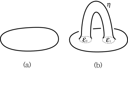
Figure 10: (a)$\Sigma$, (b)$\Sigma_{1}=(\Sigma$ with a handle attached).

The r.h.s. of (4$\cdot$17) is somewhat symbolical since the surface $\Sigma_{1}$ is not simply connected. Its meaning becomes unambiguous only after an indication of the ordering is given. Just as in the case of Eq.(4$\cdot$1), the surface $\Sigma_{1}$ can be regarded to consist of two disks $\overline{\varepsilon_{0}}$ and $\overline{\varepsilon_{1}}$, a handle $\eta$ and the surface $\Sigma$ : $\Sigma_{1}=(\overline{\varepsilon_{0}}\cup\eta\cup\overline{\varepsilon_{1}})\cup\Sigma$. The ordering for $[x(\Sigma_{1})]$ can be prescribed by

$$[x(\Sigma_{1})]=[x(\overline{\varepsilon_{0}}\cup\eta\cup\overline{\varepsilon_{1}})][x(\Sigma)].$$ (65)

Since the first factor of the r.h.s. of (4$\cdot$18) is equal to 1 as was explained below (4$\cdot$4), we are led to (4$\cdot$17).

5 Summary

In this paper we have sought the NAST for loop variables associated with nontrivial loops. It turned out that the case of the trefoil knot (Fig.1) is of fundamental importance and constitutes the building block of the general case. The NAST for this case is given by (2$\cdot$10), where the quantities $[S_{a}]$and $[S_{b}]$ appear in addition to $[S_{i}]$, $i=1,2,3,4$. Another expression of the NAST is given by (2$\cdot$13), in which the factor $[\xi]$ defined by (2$\cdot$14) appears. Thanks to the deformation invariance of $[S]$, (1$\cdot$14), and the theorem B of §4, the result does not depend on the choice of a Seifert surface of the trefoil knot. The structure of the NAST for the case of the figure eight knot (Fig.5) is the same as that of the trefoil knot since the parameter space for these two cases can be chosen homeomorphic to each other. We have seen, in sharp contrast to the Abelian case, that the loop variable $(\gamma)$ can be different from unity even if the field strength vanishes evrywhere on the surface surrounded by the loop $\gamma$. We expect that the above fact might cause some interesting physical effects.

The NAST for a generic link of genus $g$ consisting of $\mu$ connected components was simply expressed with the help of the quantities $[[*]]$ and $\{*\}$ defined by (4$\cdot$14) and (3$\cdot$11), respectively.

References

- [1] K. Wilson,Phys. Rev. D10 (1974),2445.
- [2] T. T. Wu and C. N. Yang, Phys. Rev. D12 (1975), 3845.
- [3] C. N. Yang, Phys. Rev. Lett. 33 (1974), 445.
- [4] A. M. Polyakov, Nucl. Phys. B164 (1979), 171.
- [5] C. H. Mo, P. Scharbach and T. S. Tsun, Ann. of Phys.166 (1986), 396.
- [6] L. Schlesinger, Math. Annalen 99 (1927), 413.
- [7] M. B. Halpern, Phys. Rev. D19 (1979), 517.
- [8] Y. Aref’eva, Theor. Math. Phys. 43 (1980), 353.
- [9] N. E. Bralić, Phys. Rev. D22 (1980), 3090.
- [10] P. M. Fishbane, S. Gasiorowicz and P. Kaus, Phys. Rev. D24 (1981), 2324.
- [11] L. Diósi, Phys. Rev. D27 (1983), 2552.
- [12] Yu. A. Simonov, Sov. J. Nucl. Phys. 50 (1989), 134.
- [13] B. Broda, in Advanced Electromagnetism: Foundations, Theory and Applications, ed. T. Barrett and D. Grimes (World Sci. Publ. Co, Singapore, 1995).
- [14] D. Diakonov and V. Petrov, hep-th/9606104.
- [15] M. Hirayama and S. Matsubara, Prog. Theor. Phys. 99 (1998), 691.
- [16] C. Livingston, Knot Theory (Mathematical Association of America , Washington, 1993).
- [17] S. Suzuki, Introduction to Knot Theory (Saiensu Co., Tokyo, 1991) (in Japanese).