We consider quantum dynamical systems whose degrees of freedom are described by $N\times N$ matrices, in the planar limit $N\to\infty$. Examples are gauge theories and the M(atrix)-theory of strings. States invariant under $U(N)$ are ‘closed strings’, modelled by traces of products of matrices. We have discovered that the $U(N)$-invariant operators acting on both open and closed string states form a remarkable new Lie algebra which we will call the heterix algebra. (The simplest special case, with one degree of freedom, is an extension of the Virasoro algebra by the infinite-dimensional general linear algebra.) Furthermore, these operators acting on closed string states only form a quotient algebra of the heterix algebra. We will call this quotient algebra the cyclix algebra. We express the Hamiltonian of some gauge field theories (like those with adjoint matter fields and dimensionally reduced pure QCD models) as elements of this Lie algebra. Finally, we apply this cyclix algebra to establish an isomorphism between certain planar matrix models and quantum spin chain systems. Thus we obtain some matrix models solvable in the planar limit; e.g., matrix models associated with the Ising model, the XYZ model, models satisfying the Dolan-Grady condition and the chiral Potts model. Thus our cyclix Lie algebra describes the dynamical symmetries of quantum spin chain systems, large-$N$ gauge field theories, and the M(atrix)-theory of strings.

PACS: 11.25.Hf, 11.15.Pg, 02.20.Sv, 75.10.Jm.

I Introduction

The string is emerging as a verstile concept in physics, second only to the notion of a particle in its usefulness. The instantaneous configuration of a string can be thought of roughly as a curve in space, with an energy proportional to its length. The curve may be closed, or open with some extra degrees of freedom stuck at its endpoints. The string is being intensely studied as the fundamental object in the quantum theory of gravity and perhaps even the unified theory of all forces of nature.

The modern notion of a relativistic string theory originated in attempts to understand hadron dynamics, in the sixties and early seventies. However, it is now established that Quantum Chromodynamics (QCD) is the fundamental theory of strong interactions: the hadrons are not elementary particles but instead are bound states of quarks and gluons. In spite of this, attempts to understand hadron dynamics in terms of strings have not altogether ceased. Many features of hadron dynamics which originally prompted people to construct the string theory still do not have a satisfactory explanation. For example the squares of the masses of hadrons increase linearly with their angular momenta, a characteristic property of strings. Indeed, it seems very plausible that there is a version of string theory which is equivalent to QCD but that directly describes hadrons. (Such a theory has been constructed in two dimensions [1].) Since the gluon degrees of freedom are represented by matrices, this suggests that at least this type of string can be thought of as made of more elementary entities described by products of matrices. Connections to non-commutative geometry are also natural as suggested in Ref.[2].

Meanwhile in recent years the strings that appear in theories of quantum gravity have also come to be seen as made of more elemental objects (‘string bits’ [3, 4]) again described by matrices [5, 6]. Indeed the underlying mathematical structures have much in common with earlier work on QCD with some extra symmetries (such as supersymmetry) added. These M(atrix)-theories are thought to describe not only string-like excitations but also M(embranes) and are collectively known as the M-theory. The underlying symmetries and geometrical significance of this theory still remain M(ysterious).

Both of the above applications of string theory involve fundamental degrees of freedom represented by $N\times N$ matrices. In both cases the limit $N\to\infty$ is important, as it simplifies many issues. There are in fact many inequivalent ways of letting $N$ go to infinity, the simplest one is the so-called planar large-$N$ limit. It is called as such because it was originally [7] constructed by summing Feynman diagrams which have planar topology. (Other limits such as the double scaling limit which gives the continuum string theory are of interest as well.) We view this planar limit as a linear approximation to the general large-$N$ limit discussed in Ref. [8].

Thus, the understanding of the quantum matrix models is of fundamental importance to modern theoretical physics. The two great challenges of theoretical physics — that of understanding hadron dynamics and that of developing a quantum theory of gravity — are both intertwined with the dynamics of quantum matrix models.

We have discovered the fundamental dynamical symmetry of matrix models in the large-$N$ limit: it is a remarkable new Lie algebra which we will call the heterix algebra. It is thus the algebra of symmetries that will help us solve both of the two great problems of theoretical physics. In addition, we will find a connection to a third branch of theoretical physics: we can understand the solvability of quantum spin chain models within the formalism of the heterix algebra.

The outline of this paper is as follows. In Section II, we will introduce heterix algebra axiomatically. We will also discuss aspects of its structure such as its Cartan subalgebra and root vectors. In particular, we will show that this Lie algebra is an extension of another Lie algebra by $gl_{+\infty}$ [9]. In Section III, we will study the simplest heterix algebra in which there is only one degree of freedom. It will turn out that the non-commutative algebra is simplified to the Virasoro algebra. Thus our algebra can be viewed as a generalization of the Virasoro algebra. In Section IV, we will show that gauge invariant observables in the planar large-$N$ limit can be formulated in terms of the elements of this algebra. Moreover, closed string bit states in the this large-$N$ limit provide a representation for this Lie algebra. However, this representation is not faithful and thus there are many relations among some elements of this algebra. We will quotient out these relations and get another Lie algebra — the cyclix algebra [10].

In Section V, we will discuss the applications of the cyclix algebra to various gauge field theories, which, in the planar large-$N$ limit, are multi-matrix models. In Section VI, we will construct more tractable multi-matrix models with the aid of quantum spin chain models. In addition, we will find that we can understand the solvability of quantum spin chain models within the formalism of the cyclix algebra.

II The Heterix Lie Algebra

In this section we will give a self-contained definition of a certain Lie algebra, which we will call the heterix algebra. In a latter section we will see that closed string operators provide a representation for this algebra, albeit an unfaithful one. The defining representation in this section is on the combined state space of open and closed strings and is, of course, faithful.

Define a complex vector space ${\cal T}_{op}$ of finite linear combinations of orthogonal states of an open string: $s^{L}=s^{l_{1}l_{2}\cdots l_{d}}$. This is just the space of all tensors (with no particular symmetry properties) on the complex vector space $C^{\Lambda}$:

$${\cal T}_{op}=\oplus_{r=1}^{\infty}\otimes^{r}C^{\Lambda}.$$ (1)

This vector space should be thought of as the space of states of an open string propagating in a discrete model of space-time with $\Lambda$ points. In addition define ${\cal T}_{c}$ of finite linear combinations of orthogonal states $\Psi^{(K)}=\Psi^{(k_{1}\cdots k_{c})}$ labelled by cyclically symmetric indices. Thus ${\cal T}_{c}$ is the space of cyclically symmetric tensors on $C^{\Lambda}$ and should be viewed as the space of states of a closed string propagating in discretized space. Our Lie algebra will be defined by the commutators of some operators on the total space of closed and open strings ${\cal T}={\cal T}_{c}\oplus{\cal T}_{op}$. Thus $\cal T$ has an orthogonal basis $\{\Psi^{(K)},s^{L}\}$ as $(K)$ ranges over (non-empty) equivalence classes of cyclically symmetric sequences and $L$ over all non-empty sequences. Typical open and closed string states are illustrated in Fig. 1. (The reader can compare Figs. 1(a) and (b) with Figs. 1(a) and (b) in an accompanying paper [11].)

Figure 1: (a) A typical open string state $s^{L}$ in detail. There is a series of 6 indices $l_{1}$, $l_{2}$, …, and $l_{6}$. Each index is represented by a solid bead. These solid beads are connected by thick lines (in contrast with the thin lines in latter figures). The arrow indicates the direction of the integer sequence $L$. (b) An open string state in brief. The beads are omitted. They will be consistently omitted in all ensuing brief figures. The integer sequence is represented by the letter $L$. The length of the line does not indicate the number of indices the line carries. (c) A typical closed string state $\Psi^{(K)}$ with 5 indices in detail. There is a series of indices $k_{1}$, $k_{2}$, …, and $k_{5}$. Notice the cyclic symmetry of this state. (d) A closed string state in brief. The state is represented by the equivalence class $(K)$, but in the figure we simply label the state as $K$. The size of the circle does not indicate the number of indices the circle carries.

Now let us introduce some operators that act on these states. Define the operator $\tilde{f}^{(I)}_{(J)}$ by its action on ${\cal T}$ as follows:

$$\tilde{f}^{(I)}_{(J)}\Psi^{(K)}=\delta^{K}_{(J)}\Psi^{(I)}\;\mbox{and}\;\tilde{f}^{(I)}_{(J)}s^{L}=0.$$ (2)

This operator just converts the closed string state $\Psi^{(K)}$ to $\Psi^{(I)}$, with a multiplicative factor which is the number of cyclic permutations of $K$ that is equal to $J$. It gives zero if there are no such permutations or if it acts on an open string state. Clearly $\tilde{f}^{(I)}_{(J)}$ is a finite rank operator. The operator $\tilde{f}^{(I)}_{(J)}$ is shown pictorially in Fig. 2. Also shown in the same figure is the action of $\tilde{f}^{(I)}_{(J)}$ on $\Psi^{(K)}$.

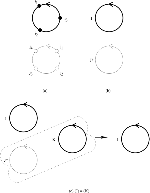
Figure 2: (a) A detailed diagrammatic representation of a typical $\tilde{f}^{(I)}_{(J)}$. The upper circle represents $(I)$, whereas the lower circle represents $(J)$. In this example, there are 3 indices in $I$ and 4 indices in $J$. An index in $I$ is represented by a solid bead, whereas an index in $J$ is represented by a hollow bead. Moreover, the solid beads are joined by thick lines, while the hollow ones are joined by thin lines. Note the sequence $J$ is put in the clockwise instead of the anti-clockwise direction. (b) $\tilde{f}^{(I)}_{(J)}$ in brief. An asterisk is added to $J$ to signify the fact that $J$ is in the anti-clockwise direction. (c) The action of $\tilde{f}^{(I)}_{(J)}$ on $\Psi^{(K)}$. The dotted lines connect the line segments to be ‘annihilated’ together. The figure on the right of the arrow is the resultant closed string state.

In addition let us define the operator $\gamma^{I}_{J}$ by its actions on closed strings —

$$\gamma^{I}_{J}\Psi^{(K)}=\delta^{K}_{(J)}\Psi^{(I)}+\sum_{K_{1}K_{2}=(K)}\delta^{K_{1}}_{J}\Psi^{(IK_{2})}$$ (3)

— and on open strings as shown:

$$\gamma^{I}_{J}s^{L}=\delta^{L}_{J}s^{I}+\sum_{L_{1}L_{2}=L}\delta^{L_{1}}_{J}s^{IL_{2}}+\sum_{L_{1}L_{2}=L}\delta^{L_{2}}_{J}s^{L_{1}I}+\sum_{L_{1}L_{2}L_{3}=L}\delta^{L_{2}}_{J}s^{L_{1}IL_{3}}.$$ (4)

Clearly, it is the direct sum of an operator $g^{I}_{J}$ acting on closed strings and $\sigma^{I}_{J}$ acting on open strings: $\gamma^{I}_{J}=g^{I}_{J}\oplus\sigma^{I}_{J}$. $\sigma^{I}_{J}$ has been defined in a previous paper [11]. These operators are not finite rank, unlike the $\tilde{f}^{(I)}_{(J)}$; indeed they are not even bounded.

Let us describe Eq.(3) in words. Regard $(K)$ as a circle of points labelled by positive integers. If $J$ has more indices than $K$, then the action of $\gamma^{I}_{J}$ on $\Psi^{(K)}$ gives zero. When $J$ is shorter than $K$, each segment of $K$ that is identical to $J$, is replaced with $I$ and then a sum over all the resultant terms is taken. This is done even if some of the segments agreeing with $J$ overlap partially with each other. If $J$ does not overlap with any segment of $K$, then we get zero.

Next, consider the case when the length of $J$ is the same as that of $K$, i.e., $\#(J)=\#(K)=c$. Then we get zero if no cyclic permutaion of $J$ agrees with $K$; otherwise, we replace $K$ with $I$ and multiply $\Phi^{(I)}$ by the number of cyclic permutataions of $K$ that agree with $J$.

Eq.(3) is illustrated in Fig. 3. Using the identities in Appendix A, Eq.(3) can be rewritten as

$$\gamma^{I}_{J}\Psi^{(K)}=\delta^{K}_{(J)}\Psi^{(I)}+\sum_{A}\delta^{K}_{(JA)}\Psi^{(IA)}.$$ (5)

This form is more convenient for some calculations.

We can understand Eq.(4) analogously. Again, if $J$ is longer than $K$, we get zero. Otherwise, each segment of $K$ that agrees with $J$ is replaced with $I$ and a sum over all such resultants is taken. The first term represents the situation when $J$ is identical to $K$; the second when J agrees with the beginning of $K$; the third when $J$ agrees with the end of $K$; the last term, which is the ‘generic’ one, describes the situation when $J$ agrees with some segment in the middle of $K$. Of course we get zero if there is no segment of $K$ that agrees with $J$. Eq.(4) is depicted in Fig. 5.

The reader can notice from the figures an analogy between the action of our operators on states and the action of some viruses on DNA molecules.

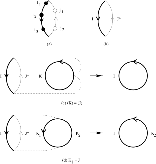
Figure 3: (a) A typical $\gamma^{I}_{J}$. There are 3 indices in $I$ and 2 indices in $J$. Note that $J$ is in reverse. (b) A concise representation of $\gamma^{I}_{J}$. Again an asterisk is added to $J$ to signify the fact that $J$ is put in reverse. (c) and (d) The action of $\gamma^{I}_{J}$ on $\Psi^{(K)}$. Only the first two terms of Eq.(3) are shown.

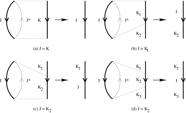
Figure 4: (a) to (d) The action of $\gamma^{I}_{J}$ on $s^{L}$ (c.f. Fig 8 in an accompanying paper [11]). Only the first four terms are shown.

Altogether, $\{\tilde{f}^{(I)}_{(J)},\gamma^{I}_{J}\}$ is a linearly independent set of operators. This fact, the proof of which can be found in Appendix B, is of some importance, as we will define a Lie algebra with this set as a basis soon. The operators $g^{I}_{J}$ acting on closed string states alone do not form a linearly independent set, however. We will derive some relations among them in a latter section.

The product of two operators $\tilde{f}^{(I)}_{(J)}\tilde{f}^{(K)}_{(L)}$ is a finite linear combination of such operators. Moreover, the $\tilde{f}^{(I)}_{(J)}$’s are linearly independent so that they span an associative algebra $\tilde{\mathit{F}}_{\Lambda}$. Their commutators span a Lie algebra which we will also call $\tilde{\mathit{F}}_{\Lambda}$. However the product $\gamma^{I}_{J}\gamma^{K}_{L}$ cannot be written in general as a finite linear combination of the $\gamma$’s and $\tilde{f}$’s. A proof of this statement can be found in Appendix C.

Nevertheless, it is a remarkable fact that the commutators of any two string-like operators defined above can in fact be written as finite linear combinations of themselves. In fact we see, by a straightforward (but tedious) computation, that the commutator between two $\gamma$’s reads

$$\left[\gamma^{I}_{J},\gamma^{K}_{L}\right]=\delta^{K}_{J}\gamma^{I}_{L}+\sum_{J_{1}J_{2}=J}\delta^{K}_{J_{2}}\gamma^{I}_{J_{1}L}+\sum_{K_{1}K_{2}=K}\delta^{K_{1}}_{J}\gamma^{IK_{2}}_{L}$$ (22)

$$+\sum_{\begin{array}[]{l}J_{1}J_{2}=J\\ K_{1}K_{2}=K\end{array}}\delta^{K_{1}}_{J_{2}}\gamma^{IK_{2}}_{J_{1}L}+\sum_{J_{1}J_{2}=J}\delta^{K}_{J_{1}}\gamma^{I}_{LJ_{2}}+\sum_{K_{1}K_{2}=J}\delta^{K_{2}}_{J}\gamma^{K_{1}I}_{L}$$

$$+\sum_{\begin{array}[]{l}J_{1}J_{2}=J\\ K_{1}K_{2}=K\end{array}}\delta^{K_{2}}_{J_{1}}\gamma^{K_{1}I}_{LJ_{2}}+\sum_{J_{1}J_{2}J_{3}=J}\delta^{K}_{J_{2}}\gamma^{I}_{J_{1}LJ_{3}}+\sum_{K_{1}K_{2}K_{3}=K}\delta^{K_{2}}_{J}\gamma^{K_{1}IK_{3}}_{L}$$

$$+\sum_{\begin{array}[]{l}J_{1}J_{2}=J\\ K_{1}K_{2}=K\end{array}}\delta^{K_{1}}_{J_{2}}\delta^{K_{2}}_{J_{1}}\tilde{f}^{(I)}_{(L)}+\sum_{\begin{array}[]{l}J_{1}J_{2}J_{3}=J\\ K_{1}K_{2}=K\end{array}}\delta^{K_{1}}_{J_{3}}\delta^{K_{2}}_{J_{1}}\tilde{f}^{(I)}_{(J_{2}L)}$$

$$+\sum_{\begin{array}[]{l}J_{1}J_{2}=J\\ K_{1}K_{2}K_{3}=K\end{array}}\delta^{K_{1}}_{J_{2}}\delta^{K_{3}}_{J_{1}}\tilde{f}^{(IK_{2})}_{(L)}$$

$$+\sum_{\begin{array}[]{l}J_{1}J_{2}J_{3}=J\\ K_{1}K_{2}K_{3}=K\end{array}}\delta^{K_{1}}_{J_{3}}\delta^{K_{3}}_{J_{1}}\tilde{f}^{(IK_{2})}_{(J_{2}L)}-(I\leftrightarrow K,J\leftrightarrow L).$$

Moreover, the commutators between a $\gamma$ and an $\tilde{f}$, and between two $\tilde{f}$’s, are

$$\left[\gamma^{I}_{J},\tilde{f}^{(K)}_{(L)}\right]=\delta^{K}_{(J)}\tilde{f}^{(I)}_{(L)}+\sum_{K_{1}K_{2}=(K)}\delta^{K_{1}}_{J}\tilde{f}^{(IK_{2})}_{(L)}-\delta^{I}_{(L)}\tilde{f}^{(K)}_{(J)}-\sum_{L_{1}L_{2}=(L)}\delta^{I}_{L_{2}}\tilde{f}^{(K)}_{(L_{1}J)}$$ (23)

and

$$\left[\tilde{f}^{(I)}_{(J)},\tilde{f}^{(K)}_{(L)}\right]=\delta^{K}_{(J)}\tilde{f}^{(I)}_{(L)}-\delta^{I}_{(L)}\tilde{f}^{(K)}_{(J)}$$ (24)

respectively. The proof of the above three equations will be relegated to Appendix D. Some terms in Eq.(22) are depicted in Figs. 5 to 7. Illustrated in Fig. 8 are the two Lie algebraic relations Eqs.(23) and (24). Let us call the Lie algebra with the basis $\{\tilde{f}^{(I)}_{(J)},\gamma^{I}_{J}\}$ and the above commutation relations the heterix algebra, $\hat{\Gamma}_{\Lambda}$.

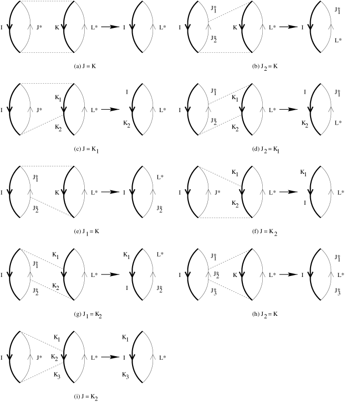
Figure 5: Diagrammatic representations of the first 9 terms on the R.H.S. of Eq.(22).

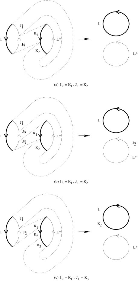
Figure 6: Diagrammatic representations of the tenth to twelfth terms on the R.H.S. of Eq.(22).

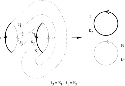
Figure 7: Diagrammatic representations of the thirteenth term on the R.H.S. of Eq.(22).

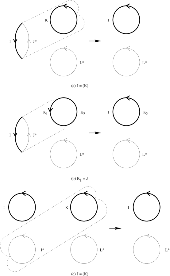
Figure 8: Diagrammatic representations of the R.H.S. of Eqs.(23) and (24). Only the first two terms and the first term are depicted in these two equations respectively.

Let us explore the structure of the heterix algebra. Fist of all, we see from Eq.(23) that $\tilde{\mathit{F}}_{\Lambda}$ is a proper ideal of the cyclix algebra. Next, consider the subspace ${\cal H}$ spanned by all vectors of the forms $\gamma^{I}_{I}$ and $\tilde{f}^{(I)}_{(I)}$, where $I$ is an arbitrary finite integer sequence of integers between 1 and $\Lambda$ inclusive. It turns out that ${\cal H}$ is a Cartan subalgebra of the heterix algebra. (The proof can be found in Appendix E.) In addition, we have the following special cases of Eq.(23) and (24):

$$\left[\gamma^{I}_{I},\tilde{f}^{(K)}_{(L)}\right]=\left(\delta^{K}_{(I)}+\sum_{K_{1}K_{2}=(K)}\delta^{K_{1}}_{I}-\delta^{I}_{(L)}-\sum_{L_{1}L_{2}=(L)}\delta^{I}_{L_{1}}\right)\tilde{f}^{(K)}_{(L)}$$ (25)

and

$$\left[\tilde{f}^{(I)}_{(I)},\tilde{f}^{(K)}_{(L)}\right]=\left(\delta^{K}_{(I)}-\delta^{I}_{(L)}\right)\tilde{f}^{(K)}_{(L)}.$$ (26)

Therefore, every $\tilde{f}^{(K)}_{(L)}$ is a root vector of the cyclix algebra with respect to the subalgebra ${\cal H}$.

Suppose we define some operators as follows:

$$l^{I}_{J} \equiv \gamma^{I}_{J}-\sum_{i=1}^{\Lambda}\gamma^{iI}_{iJ}-\tilde{f}^{(I)}_{(J)}\mbox{; and}$$

$$r^{I}_{J} \equiv \gamma^{I}_{J}-\sum_{j=1}^{\Lambda}\gamma^{Ij}_{Jj}-\tilde{f}^{(I)}_{(J)}.$$ (27)

The actions of these operators on ${\cal T}$ are:

$$l^{I}_{J}s^{K} = \delta^{K}_{J}s^{I}+\sum_{K_{1}K_{2}=K}\delta^{K_{1}}_{J}s^{IK_{2}};$$

$$l^{I}_{J}\Psi^{(K)} = 0;$$

$$r^{I}_{J}s^{K} = \delta^{K}_{J}s^{I}+\sum_{K_{1}K_{2}=K}\delta^{K_{2}}_{J}s^{K_{1}I}\mbox{; and}$$

$$r^{I}_{J}\Psi^{(K)} = 0.$$ (28)

Hence they act only on the open string states: $l^{I}_{J}$ and $r^{I}_{J}$ are precisely the operators defined in a previous paper [11] on open strings. From the results of that paper, we deduce that the algebra consisting of finite linear combinations of $l^{I}_{J}$’s, $\hat{L}^{\prime}_{\Lambda}$, is a subalgebra of the heterix algebra. Similarly, the algebra consisting of finite linear combinations of $r^{I}_{J}$’s, $\hat{R}^{\prime}_{\Lambda}$, is also a subalgebra of the cyclix algebra.

Now define

$$f^{I}_{J} \equiv \gamma^{I}_{J}-\sum_{i=1}^{\Lambda}\gamma^{iI}_{iJ}-\sum_{j=1}^{\Lambda}\gamma^{Ij}_{Jj}\sum_{i,j=1}^{\Lambda}\gamma^{iIj}_{iJj}-\tilde{f}^{(I)}_{(J)}+\sum_{i=1}^{\Lambda}\tilde{f}^{(iI)}_{(iJ)}$$ (29)

$$= l^{I}_{J}-\sum_{j=1}^{\Lambda}l^{Ij}_{Jj}$$

$$= r^{I}_{J}-\sum_{i=1}^{\Lambda}r^{iI}_{iJ}.$$

Its action on ${\cal T}$ reads

$$f^{I}_{J}s^{K} = \delta^{K}_{J}s^{I}\mbox{; and}$$

$$f^{I}_{J}\Psi^{(K)} = 0.$$ (30)

Hence this $f^{I}_{J}$ also act only on open strings; it too was introduced in Ref. [11]. The algebra consisting of finite linear combinations of $f^{I}_{J}$’s, $F^{\prime}_{\Lambda}$, is a subalgebra of $\hat{L}^{\prime}_{\Lambda}$, $\hat{R}^{\prime}_{\Lambda}$ and the heterix algebra. We deduce from Eqs.(2), (3), (4) and (30) that

$$\left[\gamma^{I}_{J},f^{K}_{L}\right]=\delta^{K}_{J}f^{I}_{L}+\sum_{K_{1}K_{2}=K}\delta^{K_{1}}_{J}f^{IK_{2}}_{L}+\sum_{K_{1}K_{2}=K}\delta^{K_{2}}_{J}f^{K_{1}I}_{L}$$

$$+\sum_{K_{1}K_{2}K_{3}=K}\delta^{K_{2}}_{J}f^{K_{1}IK_{3}}_{L}-\delta^{I}_{L}f^{K}_{J}-\sum_{L_{1}L_{2}=L}\delta^{I}_{L_{1}}f^{K}_{JL_{2}}$$

$$-\sum_{L_{1}L_{2}=L}\delta^{I}_{L_{2}}f^{K}_{L_{1}J}-\sum_{L_{1}L_{2}L_{3}=L}\delta^{I}_{L_{2}}f^{K}_{L_{1}JL_{3}}\mbox{; and}$$

$$\left[\tilde{f}^{(I)}_{(J)},f^{K}_{L}\right]=0.$$ (31)

In particular,

$$\left[\gamma^{I}_{I},f^{K}_{L}\right] = \left(\delta^{K}_{I}+\sum_{K_{1}K_{2}=K}\delta^{K_{1}}_{I}+\sum_{K_{1}K_{2}=K}\delta^{K_{2}}_{I}+\sum_{K_{1}K_{2}K_{3}=K}\delta^{K_{2}}_{I}\right.$$

$$\left.-\delta^{I}_{L}-\sum_{L_{1}L_{2}=L}\delta^{I}_{L_{1}}-\sum_{L_{1}L_{2}=L}\delta^{I}_{L_{2}}-\sum_{L_{1}L_{2}L_{3}=L}\delta^{I}_{L_{2}}\right)f^{K}_{L}\mbox{; and}$$

$$\left[\tilde{f}^{(I)}_{(I)},f^{K}_{L}\right] = 0.$$ (32)

Thus every $f^{K}_{L}$ is also a root vector with respect to the Cartan subalgebra ${\cal H}$. In fact, a root vector with respect to ${\cal H}$ is either of the form $\tilde{f}^{(K)}_{(L)}$ or $f^{K}_{L}$. The proof of this assertion can be found in Appendix F. Hence every root space is one-dimensional.

The reader can refer to Ref. [11] for a more detailed discussion of the Lie algebraic relations among the $f$’s, $l$’s, $r$’s and $\gamma$’s. Also shown in detail in the same article are various diagrammatic representations of $f$’s, $l$’s, $r$’s, and the Lie algebraic relations pertaining to them.

Now let us consider various quotient algebras from the heterix algebra. Since $\tilde{\mathit{F}}_{\Lambda}$ is a proper ideal, we can make the set of all cosets $\gamma^{I}_{J}+\tilde{\mathit{F}}_{\Lambda}$ into a quotient algebra. This quotient algebra is nothing but the centrix algebra $\hat{\Sigma}_{\Lambda}$ [11] defined previosly. The union of $\hat{L}^{\prime}_{\Lambda}$ and $\hat{R}^{\prime}_{\Lambda}$, the multix algebra $\hat{M}^{\prime}_{\Lambda}$ [11], is another proper ideal, thus we can make the set of all cosets $\gamma^{I}_{J}+\hat{M}^{\prime}_{\Lambda}$ and $\tilde{f}^{(I)}_{(J)}+\hat{M}^{\prime}_{\Lambda}$ a quotient algebra as well. Note that every operator in $\hat{M}^{\prime}_{\Lambda}$ acts on ${\cal T}_{c}$ to produce 0. We conjecture that ${\cal T}_{c}$ provides a faithful representation for the quotient algebra of all cosets $\gamma^{I}_{J}+\hat{M}^{\prime}_{\Lambda}$ and $\tilde{f}^{(I)}_{(J)}+\hat{M}^{\prime}_{\Lambda}$. As we will see in the next section, the corresponding $\Lambda=1$ quotient algebra is precisely the Virasoro algebra without any central extension. Therefore the quotient algebra with $\Lambda>1$ can be regarded as a generalization of the Virasoro algebra.

The Lie bracket of the subalgebra $\tilde{\mathit{F}}_{\Lambda}$ is given by Eq.(24). If we rescale each vector by defining

$$f^{(I)}_{(J)}\equiv\frac{\tilde{f}^{(I)}_{(J)}}{\sqrt{\delta^{I}_{(I)}\delta^{J}_{(J)}}},$$ (33)

then the Lie bracket between two $f^{(I)}_{(J)}$’s is similar to that in Eq.(24), except that the delta function there with the generic form $\delta^{I}_{(J)}$ should be replaced with another delta function such that this new delta function yields simply 1 if $(I)=(J)$, and remains 0 otherwise. Then there is a one-to-one correspondence between each $f^{(I)}_{(J)}$ and each complex matrix $(a_{ij})_{i,j}\in Z_{+}$ such that all but one $a_{ij}$ is nonzero, and that nonzero entry is 1. Thus the Lie algebras $\tilde{\mathit{F}}_{\Lambda}$, for any $\Lambda$ are all isomorphic to $gl_{+\infty}$, the inductive limit of the general linear algebras. $gl_{+\infty}$ and the Kac-Moody algebra associated with it were thoroughly studied, and their properties can be found in, e.g., Kac’s work [9].

III The special case $\Lambda=1$

Let us consider the cyclix algebra for the simplest special case $\Lambda=1$ : this is useful as it will connect our Lie algebra with more familiar algebras such as the Virasoro algebra. Then all the sequences are repetitions of the number $1$ some numbers of times. We can simplify the notations and write $\Psi^{(K)}$ as $\Psi^{(\#(K))}$, $s^{K}$ as $s^{\#(K)}$, $\gamma^{I}_{J}$ as $\gamma^{\#(I)}_{\#(J)}$ and $\tilde{f}^{(I)}_{(J)}$ as $\tilde{f}^{(\#(I))}_{(\#(J))}$. We can deduce from Eqs.(2), (3) and (4) that the actions of $\tilde{f}^{(a)}_{(b)}$ and $\gamma^{a}_{b}$, where $a$ and $b$ are the number of integers in the various sequences, on $\Psi^{(c)}$ and $s^{c}$, where $c$ is also a positive integer, is given by

$$\tilde{f}^{(a)}_{(b)}\Psi^{(c)} = c\delta^{c}_{b}\Psi^{(a)};$$ (34)

$$\tilde{f}^{(a)}_{(b)}s^{c} = 0;$$ (35)

$$\gamma^{a}_{b}\Psi^{(c)} = c\theta(b\leq c)\Psi^{(a+c-b)}\mbox{; and}$$ (36)

$$\gamma^{a}_{b}s^{c} = (c-b+1)\theta(b\leq c)s^{a+c-b}.$$ (37)

where $\theta(\mbox{{\em condition}})$ is 1 if the condition holds, and 0 otherwise. The Lie brackets for the $\Lambda=1$ cyclix algebra are

$$\left[\gamma^{a}_{b},\gamma^{c}_{d}\right] = \theta(c\leq b)\left[2\gamma^{a+c-1}_{b+d-1}+2\gamma^{a+c-2}_{b+d-2}+\cdots+2\gamma^{a+1}_{b+d-c+1}\right.$$ (38)

$$\left.+(b-c+1)\gamma^{a}_{b+d-c}\right]+\theta(2\leq c\leq b)\left[\tilde{f}^{(a+c-2)}_{(b+d-2)}+2\tilde{f}^{(a+c-3)}_{(b+d-3)}\right.$$

$$\left.+\cdots+(c-1)\tilde{f}^{(a)}_{(b+d-c)}\right]+\theta(b<c)\left[2\gamma^{a+c-1}_{b+d-1}+2\gamma^{a+c-2}_{b+d-2}\right.$$

$$\left.+\cdots+2\gamma^{a+c-b+1}_{d+1}+(c-b+1)\gamma^{a+c-b}_{d}\right]+\theta(2\leq b<c)\left[\tilde{f}^{(a+c-2)}_{(b+d-2)}\right.$$

$$\left.+\tilde{f}^{(a+c-3)}_{(b+d-3)}+\cdots+(b-1)\tilde{f}^{(a+c-d)}_{(b)}\right]$$

$$-(a\leftrightarrow c,b\leftrightarrow d);$$

$$\left[\gamma^{a}_{b},\tilde{f}^{(c)}_{(d)}\right]=c\theta(b\leq c)\tilde{f}^{(a+c-b)}_{(d)}-d\theta(a\leq d)\tilde{f}^{(c)}_{(b+d-a)}$$ (39)

and

$$\left[\tilde{f}^{(a)}_{(b)},\tilde{f}^{(c)}_{(d)}\right]=b\delta^{c}_{b}\tilde{f}^{(a)}_{(d)}-a\delta^{a}_{d}\tilde{f}^{(c)}_{(b)}.$$ (40)

These three equations can be deduced from Eqs.(22), (23) and (24) respectively.

The Cartan subalgebra ${\cal H}$ is now spanned by vectors of the forms $\gamma^{a}_{a}$ and $\tilde{f}^{(a)}_{(a)}$. A root vector reads $\tilde{f}^{(c)}_{(d)}$ or $f^{c}_{d}=\gamma^{c}_{d}-2\gamma^{c+1}_{d+1}+\gamma^{c+2}_{d+2}-\tilde{f}^{(c)}_{(d)}+\tilde{f}^{(c+1)}_{(d+1)}$. The expression for $f^{c}_{d}$ can be deduced from Eq.(29). The eigenequations are

$$\left[\gamma^{a}_{a},\tilde{f}^{(c)}_{(d)}\right] = \left(c\theta(a\leq c)-d\theta(a\leq d)\right)\tilde{f}^{(c)}_{(d)};$$

$$\left[\tilde{f}^{(a)}_{(a)},\tilde{f}^{(c)}_{(d)}\right] = a\left(\delta^{c}_{a}-\delta^{a}_{d}\right)\tilde{f}^{(c)}_{(d)};$$

$$\left[\gamma^{a}_{a},f^{c}_{d}\right] = \left(\theta(a\leq c)(c-a+1)-\theta(a\leq d)(d-a+1)\right)f^{c}_{d}\mbox{; and}$$ (41)

$$\left[\tilde{f}^{(a)}_{(a)},f^{c}_{d}\right] = 0.$$ (42)

Let us consider the quotient algebra of all cosets $\gamma^{a}_{b}+\hat{M}^{\prime}_{1}$ and $\tilde{f}^{(a)}_{(b)}+\hat{M}^{\prime}_{1}$. In the rest of this section and in the accompanying appendices, we will write $\gamma^{a}_{b}+\hat{M}^{\prime}_{1}$ and $\tilde{f}^{(a)}_{(b)}+\hat{M}^{\prime}_{1}$ simply as $g^{a}_{b}$ and $\tilde{f}^{(a)}_{(b)}$ respectively. ${\cal T}_{c}$ still provides a representation for this quotient algebra — the actions of $g^{a}_{b}$ and $\tilde{f}^{(a)}_{(b)}$ on ${\cal T}_{c}$ are still described by Eqs.(34) and (36). However, there is now a relation among $\tilde{f}$’s and $g$’s:

$$\tilde{f}^{(a)}_{(b)}=g^{a}_{b}-g^{a+1}_{b+1}.$$ (43)

Hence,

$$g^{a}_{b}=\left\{\begin{array}[]{ll}-\tilde{f}^{(a)}_{(b)}-\tilde{f}^{(a-1)}_{(b-1)}-\cdots-\tilde{f}^{(a-b+1)}_{(1)}+g^{a-b+1}_{1}&\mbox{if $a\geq b$; and}\\ -\tilde{f}^{(a)}_{(b)}-\tilde{f}^{(a-1)}_{(b-1)}-\cdots-\tilde{f}^{(1)}_{(b-a+1)}+g^{1}_{b-a+1}&\mbox{if $a<b$.}\end{array}\right.$$ (44)

A simplification brought about by setting $\Lambda$ to 1 is that we can write a basis for the quotient algebra easily. Indeed, the set of all $\tilde{f}^{(a)}_{(b)}$’s, $g^{1}_{b}$’s and $g^{a}_{1}$’s where $a$ and $b$ are arbitrary positive integers form a basis for the $\Lambda=1$ quotient algebra. The proof of this statement will be given in Appendix G. The same proof also shows that ${\cal T}_{c}$ provides not only a representation, but also a faithful representation for this quotient algebra. From Eq.(39), we deduce that the subspace $\tilde{\mathit{F}}_{1}^{\prime}$ spanned by all the vectors of the form $\tilde{f}^{(c)}_{(d)}$ form a proper ideal of this quotient algebra.

The set of all $\tilde{f}^{(a)}_{(a)}$’s, where $a$ is arbitrary, and $g^{1}_{1}$ form a basis for a Cartan subalgebra. The proof of this statement will be seen in Appendix H. In addition, since $\tilde{\mathit{F}}_{1}^{\prime}$ is a proper ideal of the quotient algebra, the same proof reveals that any root vector with respect to this Cartan subalgebra must be a linear combination of a number of $\tilde{f}^{(a)}_{(b)}$’s. Therefore all root vectors are of the form $\tilde{f}^{(c)}_{(d)}$’s with $c\neq d$. The corresponding eigenequations, which can be deduced from Eqs.(25) and (26), are

$$\left[g^{1}_{1},\tilde{f}^{(c)}_{(d)}\right]=\left(c-d\right)\tilde{f}^{(c)}_{(d)}$$ (45)

and

$$\left[\tilde{f}^{(a)}_{(a)},\tilde{f}^{(c)}_{(d)}\right]=a\left(\delta^{c}_{a}-\delta^{a}_{d}\right)\tilde{f}^{(c)}_{(d)}.$$ (46)

As $\tilde{\mathit{F}}_{1}^{\prime}$ is a proper ideal of this $\Lambda=1$ quotient algebra, we can form yet another quotient algebra of cosets of the form $v+\tilde{\mathit{F}}_{1}^{\prime}$ where $v$ is an arbitrary vector of the previous quotient algebra. This new quotient algebra is spanned by the cosets $g^{a}_{1}+\tilde{\mathit{F}}_{\Lambda}$ and $g^{1}_{b}+\tilde{\mathit{F}}_{1}^{\prime}$, where $a$ and $b$ run over all positive integers. It is a straightforward matter to show that the following Lie brackets are true:

$$\left[g^{a}_{1}+\tilde{\mathit{F}}_{1}^{\prime},g^{c}_{1}+\tilde{\mathit{F}}_{1}^{\prime}\right] = (c-a)\left(g^{a+c-1}_{1}+\tilde{\mathit{F}}_{1}^{\prime}\right);$$

$$\left[g^{a}_{1}+\tilde{\mathit{F}}_{1}^{\prime},g^{1}_{d}+\tilde{\mathit{F}}_{1}^{\prime}\right] = \left\{\begin{array}[]{ll}(2-a-d)\left(g^{a-d+1}_{1}+\tilde{\mathit{F}}_{1}^{\prime}\right)&\mbox{if $d\leq a$, or}\\ (2-a-d)\left(g^{1}_{d-a+1}+\tilde{\mathit{F}}_{1}^{\prime}\right)&\mbox{if $a\leq d$; and}\end{array}\right.$$ (49)

$$\left[g^{1}_{b}+\tilde{\mathit{F}}_{1}^{\prime},g^{1}_{d}+\tilde{\mathit{F}}_{1}^{\prime}\right] = (b-d)\left(g^{1}_{b+d-1}+\tilde{\mathit{F}}_{1}^{\prime}\right).$$ (50)

Let us define

$$L_{a}=\left\{\begin{array}[]{ll}-g^{a+1}_{1}+\tilde{\mathit{F}}_{1}^{\prime}&\mbox{if $a\geq 0$, and}\\ -g^{1}_{1-a}+\tilde{\mathit{F}}_{1}^{\prime}&\mbox{if $a\leq 0$.}\end{array}\right.$$ (51)

Note that the $L$ here is not an integer sequence. Then Eq.(50) becomes

$$\left[L_{a},L_{b}\right]=(a-b)L_{a+b}.$$ (52)

The reader can notice at once that this is the Lie algebraic relation of the Virasoro algebra without any central element [13]. Consequently, the $\Lambda=1$ quotient algebra of all cosets $\gamma^{a}_{b}$ and $\tilde{f}^{(a)}_{(b)}$ can be regarded as an extension of the Virasoro algebra by an algebra isomorphic to $gl_{+\infty}$. The quotient algebras $\gamma^{I}_{J}+\hat{M}^{\prime}_{\Lambda}+\tilde{\mathit{F}}_{\Lambda}$ for $\Lambda>1$ can then be regarded as generalizations of the Virasoro algebra, as stated in the previous section.

IV Canonical Realization

We have presented the operators acting on strings somewhat abstractly in the last section. Although the diagrammatic descriptions give the definitions of the operators a natural motivation, it would be better to have a more direct derivation of these relations in terms of more familiar operators such as those satisfying Canonical Commutation Relations.

Let us define some bosonic operators which satisfy the Canonical Commutation Relations:

$$[a^{\mu_{1}}_{\mu_{2}}(k_{1}),a^{\dagger\mu_{3}}_{\mu_{4}}(k_{2})] = \delta_{k_{1}k_{2}}\delta^{\mu_{1}}_{\mu_{4}}\delta^{\mu_{3}}_{\mu_{2}};$$

$$[a^{\mu_{1}}_{\mu_{2}}(k_{1}),a^{\mu_{3}}_{\mu_{4}}(k_{2})] = 0\mbox{; and}$$

$$[a^{\dagger\mu_{1}}_{\mu_{2}}(k_{1}),a^{\dagger\mu_{3}}_{\mu_{4}}(k_{2})] = 0;$$ (53)

These operators create and annihilate ‘gluons’, the most fundamental entities in our theory. The name ‘gluons’ comes from the application our theory to regularized QCD, in which case these operators act on gluons. The indices $\mu,\nu$ and $\upsilon=1,2,\ldots,N$ label a quantum number we will call ‘color’. In this context, $\Lambda$ is the possible number of distinct quantum states of a gluon excluding color. These quantum states are denoted by the numbers 1, 2, …, $\Lambda$.

We identify the closed string states with a ring of gluons:

$$\Psi^{(K)}|0\rangle\equiv N^{-c/2}a^{\dagger\upsilon_{2}}_{\upsilon_{1}}(k_{1})a^{\dagger\upsilon_{3}}_{\upsilon_{2}}(k_{2})\cdots a^{\dagger\upsilon_{1}}_{\upsilon_{c}}(k_{c})|0\rangle,$$ (54)

where $c=\#(K)$. (The summation convention for color indices is implicit in the above and following expressions.) A factor of $N^{-c/2}$ is inserted so that the state has a finite norm in the large-$N$ limit. (Now the beads and connecting lines in Fig. 1(c) acquire some extra meanings — a solid bead represents a creation operator. Two beads connected by a line represents that the two corresponding creation operators share a common color index. This index is being summed over.)

We will now look at the operators which can map the above single glueball states to linear combinations of such states. In general they could also create states with several glueballs but their amplitudes are suppressed by terms of order at least $1\over N$: this fact is rather well known [3] and is a reflection in the Hamiltonian formalism of the planarity of Feynman diagrams in perturbation theory [7]. As an alternative to reading the relevant papers cited above, the reader can also consult and adapt an argument in a paper by one of us [14], where an operator in the large-$N$ limit is shown to propagate a single meson state to a linear combination of single meson states only.

There are two classes of such operators:

$$\tilde{f}^{(I)}_{(J)} \equiv N^{-(a+b)/2}a^{\dagger\mu_{2}}_{\mu_{1}}(i_{1})a^{\dagger\mu_{3}}_{\mu_{2}}(i_{2})\cdots a^{\dagger\mu_{1}}_{\mu_{a}}(i_{a})$$ (55)

$$a^{\nu_{b}}_{\nu_{1}}(j_{b})a^{\nu_{b-1}}_{\nu_{b}}(j_{b-1})\cdots a^{\nu_{1}}_{\nu_{2}}(j_{1}).$$

and

$$\gamma^{I}_{J} \equiv N^{-(a+b-2)/2}a^{\dagger\mu_{2}}_{\mu_{1}}(i_{1})a^{\dagger\mu_{3}}_{\mu_{2}}(i_{2})\cdots a^{\dagger\nu_{b}}_{\mu_{a}}(i_{a})$$ (56)

$$a^{\nu_{b-1}}_{\nu_{b}}(j_{b})a^{\nu_{b-2}}_{\nu_{b-1}}(j_{b-1})\cdots a^{\mu_{1}}_{\nu_{1}}(j_{1}).$$

These operators can act on a gluon segment of a glueball. (Now Figs. 2 and 3 can be regarded as illustrations of these operators. The solid beads represent creation operators, whereas the hollow beads represent annihilation operators. A connecting line, regardless of thickness, symbolizes the fact that the two corresponding operators share a common color index, and this index is being summed over.)

In the large-$N$ limit, such operators propagate single glueball states to linear combinations of single glueball states:

$$\tilde{f}^{(I)}_{(J)}\Psi^{(K)}=\delta^{K}_{(J)}\Psi^{(I)}$$

and

$$\gamma^{I}_{J}\Psi^{(K)}=\delta^{K}_{(J)}\Psi^{(I)}+\sum_{K_{1}K_{2}=(K)}\delta^{K_{1}}_{J}\Psi^{(IK_{2})}.$$

These are just the formulae (Eqs.(2) and (3)) we had in the previous section. Thus we have a representation of the Lie algebra of the last section on glueball states.

The representation we have obtained is however not faithful: we are only considering closed string states here. To emphasize this fact we will denote the operator acting on closed string states alone by $g^{I}_{J}$. (We would have a faithful representation if we included the open string states as well, but in this paper we will not consider them.) Indeed, using Eqs.(3) and (2), the reader can show that the following relations hold:

$$\tilde{f}^{(I)}_{(J)} = g^{I}_{J}-\sum_{k=1}^{\Lambda}g^{Ik}_{Jk}$$

$$\tilde{f}^{(I)}_{(J)} = g^{I}_{J}-\sum_{k=1}^{\Lambda}g^{kI}_{kJ}$$

$$\tilde{f}^{(I)}_{(J)} = g^{I_{2}I_{1}}_{J}-\sum_{k=1}^{\Lambda}g^{I_{2}I_{1}k}_{Jk}\;\mbox{if $I_{1}I_{2}=I$;}$$

$$\tilde{f}^{(I)}_{(J)} = g^{I_{2}I_{1}}_{J}-\sum_{k=1}^{\Lambda}g^{kI_{2}I_{1}}_{kJ}\;\mbox{if $I_{1}I_{2}=I$;}$$

$$\tilde{f}^{(I)}_{(J)} = g^{I}_{J_{2}J_{1}}-\sum_{k=1}^{\Lambda}g^{Ik}_{J_{2}J_{1}k}\;\mbox{if $J_{1}J_{2}=J$;}$$

$$\tilde{f}^{(I)}_{(J)} = g^{I}_{J_{2}J_{1}}-\sum_{k=1}^{\Lambda}g^{kI}_{kJ_{2}J_{1}}\;\mbox{if $J_{1}J_{2}=J$;}$$

$$\tilde{f}^{(I)}_{(J)} = g^{I_{2}I_{1}}_{J_{2}J_{1}}-\sum_{k=1}^{\Lambda}g^{I_{2}I_{1}k}_{J_{2}J_{1}k}\;\mbox{if $I_{1}I_{2}=I$ and $J_{1}J_{2}=J$; and}$$

$$\tilde{f}^{(I)}_{(J)} = g^{I_{2}I_{1}}_{J_{2}J_{1}}-\sum_{k=1}^{\Lambda}g^{kI_{2}I_{1}}_{kJ_{2}J_{1}}\;\mbox{if $I_{1}I_{2}=I$ and $J_{1}J_{2}=J$}.$$ (57)

These relations are generalizations of Eq.(43).

The quotient of the heterix algebra by the kernel of this representation was called the cyclix algebra [10] $\hat{C}_{\Lambda}$. As have been stated in a previous section, we conjecture that $\hat{C}_{\Lambda}=\hat{\Gamma}_{\Lambda}/\hat{M}^{\prime}_{\Lambda}$. The results in Section III shows that this conjecture is true for $\Lambda=1$.

V Application to Gauge Field Theory

We are going to apply the cyclix algebra to physical models which can be formulated as matrix models in the large-$N$ limit. In this section, we will concentrate on gauge field theories in the large-$N$ limit. We will find that we can express the physical observables of these theories in terms of the elements of the cyclix algebra. (Indeed, we will see in a future paper [15] that closed superstring models and M-theory can be formulated in terms of the supersymmetric generalization of the cyclix algebra in a similar manner.) However, they will look complicated. In the next section, we will construct multi-matrix models integrable in the large-$N$ limit associated with integrable quantum spin chain models satisfying the periodic boundary condition. Studying the ways these multi-matrix models are solved can shed light on how the more complicated gauge field theories are solved.

In this section we will let the regulator $\Lambda\to\infty$, so that the momentum indices will take an infinite number of values. In order that the previous discussions of our algebra apply directly here, we will need to regularize the field theory such that the momentum variables can take only a finite number $\Lambda$ of distinct values. But this is mostly a technicality, since we will only talk of field theories without divergences for which the limit $\Lambda\to\infty$ should exist: dimensional reductions of gauge theory to 1+1 dimesnions. The deeper problem of describing renormalizable field theories this way is being studied.

The first gauge field model is a (1+1)-dimensional SU($N$) gauge theory coupled to bosonic matter in the adjoint representation. This model has been studied by Dalley and Klebanov [16] in detail and so we will only give a brief account here. Let $g$ be the strong coupling constant, $\alpha$ and $\beta$ be ordinary spacetime indices, $A_{\alpha}$ be a gauge potential and $\phi$ be a scalar field in the adjoint representation of the gauge group $U(N)$. Both $\phi$ and $A_{\alpha}$ are $N\times N$ Hermitian matrix fields. (We can regard both $A_{\alpha}$ and $\phi$ as describing the gluons of a Yang-Mills theory in three dimensions, dimensionally reduced to 1+1 dimensions.) Let the covariant derivative $D_{\alpha}\phi=\partial_{\alpha}\phi+{\rm i}[A_{\alpha},\phi]$ and the Yang-Mills field $F_{\alpha\beta}=\partial_{\alpha}A_{\beta}-\partial_{\beta}A_{\alpha}+{\rm i}[A_{\alpha},A_{\beta}]$. Lastly, let $m$ be the mass of a boson and $g$ be the gauge field coupling strength. Then the Minkowski space action is

$$S=\int d^{2}x\,{\rm Tr}\left[\frac{1}{2}D_{\alpha}\phi D^{\alpha}\phi-\frac{1}{2}m^{2}\phi^{2}-\frac{1}{4g^{2}}F_{\alpha\beta}F^{\alpha\beta}\right].$$ (58)

We then transform the Minkowski coordinates to light-cone coordinates, and choose the light-cone gauge $A_{-}=(A_{0}-A_{3})/\sqrt{2}=0$. Then $A_{+}$ is not dynamical and can be eliminated by the constrained equations. We canonically quantize the adjoint matter field:

$$\phi^{\mu}_{\nu}(x^{+}=0)=\frac{1}{\sqrt{2\pi}}\int_{0}^{\infty}\frac{dk^{+}}{\sqrt{2k^{+}}}\left[a^{\mu}_{\nu}(k^{+}){\rm e}^{-{\rm i}k^{+}x^{-}}+a^{\dagger\mu}_{\nu}(k^{+}){\rm e}^{{\rm i}k^{+}x^{-}}\right]$$ (59)

where $\mu$ and $\nu$ are color indices. The creation and annihilation operators satisfy the Canonical Commutation Relation Eq.(53). One of the constraints dictate that the Hilbert space on which the creation and annihilation operators act be spanned by color singlet states:

$$N^{-c/2}{\rm Tr}\left[a^{\dagger}(k_{1}^{+})\cdots a^{\dagger}(k_{c}^{+})\right]|0\rangle.$$ (60)

Eq.(60) is exactly in the form of a single glueball state $\Psi^{(K)}|0\rangle$ defined in Eq.(54). Thus the creation operator can be interpreted as a creation operator for a gluon. Furthermore, We can obtain the light-cone momentum and energy in terms of the elements of the cyclix algebra:

$$P^{+} = \int_{0}^{\infty}dk\;kg^{k}_{k}\mbox{; and}$$ (61)

$$P^{-} = \frac{1}{2}m^{2}\int_{0}^{\infty}\frac{dk}{k}g^{k}_{k}+\frac{g^{2}N}{4\pi}\int_{0}^{\infty}\frac{dk}{k}Cg^{k}_{k}$$ (62)

$$+\frac{g^{2}N}{8\pi}\int_{0}^{\infty}\frac{dk_{1}dk_{2}dk_{3}dk_{4}}{\sqrt{k_{1}k_{2}k_{3}k_{4}}}\left\{A\delta(k_{1}+k_{2}-k_{3}-k_{4})g^{k_{1}k_{2}}_{k_{3}k_{4}}\right.$$

$$+B\delta(k_{1}-k_{2}-k_{3}-k_{4})g^{k_{1}}_{k_{2}k_{3}k_{4}}$$

$$+\left.B\delta(k_{1}+k_{2}+k_{3}-k_{4})g^{k_{1}k_{2}k_{3}}_{k_{4}}\right\}$$

where

$$A = \frac{(k_{2}-k_{1})(k_{4}-k_{3})}{(k_{1}+k_{2})^{2}}-\frac{(k_{3}+k_{1})(k_{4}+k_{2})}{(k_{4}-k_{2})^{2}};$$

$$B = \frac{(k_{1}+k_{4})(k_{3}-k_{2})}{(k_{3}+k_{2})^{2}}+\frac{(k_{3}+k_{4})(k_{1}-k_{2})}{(k_{1}+k_{2})^{2}}\mbox{; and}$$

$$C = \int_{0}^{k}dp\frac{(k+p)^{2}}{p(k-p)^{2}}.$$

This adjoint matter model can be used to study glueball spectrum [17]. Consider next a (3+1)-dimensional QCD model with only gluons and no quarks. If we apply the dimensional reduction to it, we will obtain an effective Yang-Mills model in 1+1 dimensions with 2 adjoint matter fields $\phi_{1}$ and $\phi_{2}$, which are constant multiples of transverse gluon fields. Rewrite the adjoint matter fields in the helicity basis

$$\phi_{\pm}=\frac{\phi_{1}\pm{\rm i}\phi_{2}}{\sqrt{2}},$$ (63)

and canonically quantize $\phi_{\pm}$:

$$\phi^{\mu}_{\pm\nu}(x^{+}=0)=\frac{1}{\sqrt{2\pi}}\int_{0}^{\infty}\frac{dk^{+}}{\sqrt{2k^{+}}}\left[a^{\mu}_{\nu}(k^{+},\pm){\rm e}^{-{\rm i}k^{+}x^{-}}+a^{\dagger\mu}_{\nu}(k^{+},\pm){\rm e}^{{\rm i}k^{+}x^{-}}\right].$$ (64)

Then the light-front momentum and energy are

$$P^{+} = \int_{0}^{\infty}dk\;k\sum_{j=+,-}g^{k,j}_{k,j}\mbox{; and}$$

$$P^{-} = \frac{m_{\mbox{ind}}^{2}}{2}\int_{0}^{\infty}\frac{dk}{k}g^{k,+}_{k,+}+\frac{g^{2}}{8\pi}\int_{0}^{\infty}\frac{dk_{1}dk_{2}dk_{3}dk_{4}}{\sqrt{k_{1}k_{2}k_{3}k_{4}}}\delta(k_{1}+k_{2}-k_{3}-k_{4})\cdot$$ (65)

$$\left\{(D[k_{1},k_{2},k_{3}]-1)g^{k_{3},+;k_{4},-}_{k_{1},-;k_{2},+}+(-E[k_{1},k_{2},k_{3}]-1)g^{k_{3},+;k_{4},+}_{k_{1},+;k_{2},+}\right.$$

$$\left.+(D[k_{1},k_{2},k_{3}]-E[k_{1},k_{2},k_{3}]+2)g^{k_{3},+;k_{4},-}_{k_{1},+;k_{2},-}\right\}$$

$$+\frac{g^{2}}{8\pi}\int_{0}^{\infty}\frac{dk_{1}dk_{2}dk_{3}dk_{4}}{\sqrt{k_{1}k_{2}k_{3}k_{4}}}\delta(k_{1}+k_{2}+k_{3}-k_{4})\cdot$$

$$\left\{(F[k_{1},k_{2},k_{3}]+1)(g^{k_{1},+;k_{2},-;k_{3},+}_{k_{4},+}+g^{k_{3},+;k_{2},-;k_{1},+}_{k_{4},+}+g^{k_{4},+}_{k_{1},+;k_{2},-;k_{3},+}\right.$$

$$+g^{k_{4},+}_{k_{3},+;k_{2},-;k_{1},+})$$

$$+(F[k_{1},k_{2},k_{3}]-1)(g^{k_{3},-;k_{2},-;k_{1},+}_{k_{4},-}+g^{k_{1},+;k_{2},-;k_{3},-}_{k_{4},-}+g^{k_{4},+}_{k_{3},+;k_{2},+;k_{1},-}$$

$$\left.+g^{k_{4},+}_{k_{1},-;k_{2},+;k_{3},+})\right\}$$

$$+(\mbox{positive helicity}\leftrightarrow\mbox{negative helicity})$$

where

$$E[x_{1},x_{2},x_{3}] = \frac{(x_{1}+x_{3})(x_{1}+2x_{2}-x_{3})}{(x_{1}-x_{3})^{2}};$$

$$D[x_{1},x_{2},x_{3}] = E[x_{2},-x_{3},-x_{1}]\mbox{; and}$$

$$F[x_{3},x_{2},x_{1}] = E[x_{3},x_{1},-x_{2}],$$

and $m_{\mbox{ind}}$ is the induced mass due to normal-ordering the creation and annihilation operators.

The various algebras described in this paper can also be modified to study supersymmetric models with fermionic adjoint matter fields. Not long ago there were studies on $d>2$ noncritical superstrings using a matrix model [18]. The superfields were presented as matrices. Canonical quantization yielded a number of operators satisfying various canonical commutation and anticommutation relations. The Hilbert space on which these operators acted were composed of closed strings of bosonic and fermionic creation operators. The terms in the supercharge operators could be written in a way analogous to the gluonic operators, except that there were fermionic operators in addition to bosonic operators, which are the only operators present in the gluonic operators defined in Eq.(56). The various algebras described in this paper can be generalized to superalgebras [15] to study this noncritical superstring model. A closely related model is a supersymmetric Yang-Mills theory with a fermionic matter field [16, 19]. Moreover, these superalgebras can also be employed to study M-theory, which is being conjectured as a matrix model [5].

VI Solvable Matrix And Spin Chain Models

Now that we have learnt how to formulate gauge field theories in the large-$N$ limit in the language of the cyclix algebra, let us turn to integrable periodic quantum spin chain models and the associated, more tractable multi-matrix models. Understanding the properties of these solvable matrix models may shed new light on the mathematics of the more difficult gauge field theories.

Consider the Hamiltonian of a matrix model in the form of the linear combination $H=\sum_{IJ}h^{J}_{I}g^{I}_{J}$ where $h^{J}_{I}\neq 0$ only if $I$ and $J$ have the same number of indices. (This means that the ‘parton number’ is conserved. Note that the gauge field theories described in the previous section are not of this type.) Such linear combinations form a subalgebra of the cyclix algebra. Let us call this $\hat{C}^{0}_{\Lambda}$.

There is an isomorphism between multi-matrix models whose Hamiltonians are in $\hat{C}^{0}_{\Lambda}$ and periodic quantum spin chains. Consider a spin chain with $c$ sites. At any site $p=1,2$, …, or $c$ there is a variable $i_{p}$ called spin that describes the quantum state of that site, and that can take the value 1, 2, …, or $\Lambda$. We impose the periodic boundary condition. We will show that a subspace of these states, namely, the states with zero total momentum, provides a (non-faithful) representation of the algebra $\hat{C}^{0}_{\Lambda}$.

A basis of states is given by the set of states of the form $|k_{1}k_{2}\ldots k_{c}\rangle$. Define the operator $X^{i}_{j}(p)$ by its action on these collective spin chain states by the formula

$$X^{i}_{j}(p)|k_{1}k_{2}\ldots k_{c}\rangle\equiv\delta^{k_{p}}_{j}|k_{1}k_{2}\ldots k_{p-1}ik_{p+1}\ldots k_{c}\rangle.$$ (66)

(Those who are familiar with the theory of the Hubbard model can notice at once that $X^{i}_{j}(p)$ is the Hubbard operator at the site $p$, which is conventionally written as $X^{ij}_{p}$ [20].) Furthermore, we impose the periodic boundary condition $X^{i}_{j}(p+c)=X^{i}_{j}(p)$. It can be verified that if $I$ and $J$ have the same length $a\leq c$, then

$$r_{c}(g^{I}_{J})\equiv\sum_{p=1}^{c}X^{i_{1}}_{j_{1}}(p)X^{i_{2}}_{j_{2}}(p+1)\cdots X^{i_{a}}_{j_{a}}(p+a-1)$$ (67)

satisfies the commutation relations of the algebra $\hat{C}^{0}_{\Lambda}$. If we further define $r_{c}(g^{I}_{J})=0$ for $a>c$, we will have a representation $r_{c}$ of $\hat{C}^{0}_{\Lambda}$. The cyclically symmetric states of the matrix model correspond to the states of the periodic spin chain with zero total momentum. The representation is not faithful as it is sets all generators of length $a$ greater than the number of spins $c$ to zero; if we take spin chains of all possible lengths, we will get a faithful representation.

We are now ready to associate the matrix model which the Hamiltonian $H=\sum_{IJ}h^{J}_{I}g^{I}_{J}$ is in $\hat{C}^{0}_{\Lambda}$, with the quantum spin chain with the Hamiltonian

$$H^{{\rm spin}}=\sum_{IJ}h^{J}_{I}\sum_{p=1}^{c}X^{i_{1}}_{j_{1}}(p)X^{i_{2}}_{j_{2}}(p+1)\cdots X^{i_{a}}_{j_{a}}(p+a-1).$$ (68)

Therefore, matrix models conserving the parton number correspond to quantum spin systems with interactions involving neighborhoods of spins at the sites $p$, $p+1$, …, and $p+a-1$.

Recall that a convenient way of solving spin chain systems [21] is via the Bethe ansatz. This ansatz is applicable whenever the spin wave S-matrix satisfies the Yang-Baxter equation, in which case we say that the spin chain system is integrable. Then this integrable spin chain system yield an integrable multi-matrix model.

Let us look at the simplest example, the quantum Ising spin chain [22, 23]. The Hamiltonian $H^{\rm spin}_{\rm Ising}$ of this model is

$$H^{\rm spin}_{\rm Ising}(\tau,\lambda)=\sum_{p=1}^{c}\tau^{z}(p)+\lambda\sum_{p=1}^{c}\tau^{x}(p)\tau^{x}(p+1).$$ (69)

Here $\lambda$ is a constant, and $\tau^{x,y,z}_{p}$ are Pauli matrices at site $p$. Two Pauli matrices at different sites (i.e., with different subscripts) commute with each other. Let us rewrite the Ising spin chain as a two-matrix model. We set the quantum state 1 for a boson in the matrix model to correspond to the spin-up state in the Ising spin chain, and the quantum state 2 to correspond to the spin-down state. Since

$$\tau^{z}_{p}=X^{1}_{1}(p)-X^{2}_{2}(p),\;\tau^{x}_{p}+{\rm i}\tau^{y}_{p}=2X^{1}_{2}(p)\;\mbox{and}\;\tau^{x}_{p}-{\rm i}\tau^{y}_{p}=2X^{2}_{1}(p),$$ (70)

we obtain the corresponding element in $\hat{C}^{0}_{2}$:

$$H^{\rm matrix}_{\rm Ising}=H_{0}+\lambda V$$ (71)

where

$$H_{0} = g^{1}_{1}-g^{2}_{2}\mbox{; and}$$

$$V = \lambda\left[g^{22}_{11}+g^{21}_{12}+g^{12}_{21}+g^{11}_{22}\right].$$ (72)

This is a two-matrix model with the Hamiltonian

$$H^{\rm matrix}_{\rm Ising} = {\rm tr}[a^{{\dagger}}(1)a(1)-a^{{\dagger}}(2)a(2)]+{\lambda\over N}{\rm tr}\left[a^{{\dagger}}(2)a^{{\dagger}}(2)a(1)a(1)\right.$$ (73)

$$+a^{{\dagger}}(2)a^{{\dagger}}(1)a(2)a(1)+a^{{\dagger}}(1)a^{{\dagger}}(2)a(1)a(2)$$

$$\left.+a^{{\dagger}}(1)a^{{\dagger}}(1)a(2)a(2)\right].$$

Our results, along with known results of the Ising spin chain [23], give the spectrum of this matrix model in the large $N$ limit:

$$E(n_{p},c,\lambda)=-2\sum_{p=-c}^{c}\Bigg{(}1+2\lambda\cos\big{[}{2\pi p\over 2c+1}\big{]}+\lambda^{2}\Bigg{)}^{1/2}n_{p}$$ (74)

where $c$ is any positive integer and $n_{p}=0$ or 1. Also, we must impose the condition $\sum_{p=-c}^{c}n_{p}p=0$ to get cyclically symmetric states. Let us underscore that the matrix model defined by the Hamiltonian $H^{{\rm matrix}}_{\rm Ising}$ in Eqs.(72) or (73) is an integrable matrix model in the large-$N$ limit.

Eq.(74) manifests the self-duality of the Ising model:

$$E(n_{p},c,\lambda)=\lambda E(n_{p},c,\frac{1}{\lambda}).$$ (75)

Indeed, under the operator dual transformation

$$\tilde{\tau}^{x}(p) \equiv \tau^{z}(p)\tau^{z}(p+1)\;\mbox{and}$$

$$\tilde{\tau}^{z}(p) \equiv \tau^{x}(1)\tau^{x}(2)\cdots\tau^{x}(p),$$ (76)

the Hamiltonian is changed to

$$H^{\rm spin}_{\rm Ising}(\tilde{\tau},\lambda)=\sum_{p=1}^{c}\tilde{\tau}^{x}(p)\tilde{\tau}^{x}(p+1)+\lambda\sum_{p=1}^{c}\tilde{\tau}^{z}(p).$$ (77)

Since $\tilde{\tau}^{x}(p)$’s and $\tilde{\tau}^{z}(p)$’s satisfy the same algebra as $\tau^{x}(p)$’s and $\tau^{z}(p)$’s,

$$H^{\rm spin}_{\rm Ising}(\tilde{\tau},\lambda)=\lambda H^{\rm spin}_{\rm Ising}(\tau,\frac{1}{\lambda}),$$ (78)

i.e., the Ising model is self-dual.

It is possible to understand the solvability of the Ising model in terms of the Dolan-Grady conditions [24, 25] and the Onsager algebra. Let us digress to summarize this method. Suppose we have a system whose hamiltonian can be written as

$$H=H_{0}+V$$ (79)

with the two terms in the hamiltonian satisfying the Dolan-Grady conditions:

$$[H_{0},[H_{0},[H_{0},V]]]=16[H_{0},V],$$ (80)

and

$$[V,[V,[V,H_{0}]]]=16[V,H_{0}].$$ (81)

Then we can construct operators satisfying an infinite-dimensional Lie algebra

$$[A_{m},A_{n}]=4G_{m-n},\;[G_{m},A_{n}]=2A_{n+m}-2A_{n-m},\;\mbox{and}\;[G_{m},G_{n}]=0$$ (82)

by the following recursion relations:

$$A_{0}=H_{0},\;A_{1}=V,\;A_{n+1}-A_{n-1}=\frac{1}{2}[G_{1},A_{n}],$$

$$G_{1}=\frac{1}{4}[A_{1},A_{0}],\;\mbox{and}\;G_{n}=\frac{1}{4}[A_{n},A_{0}].$$ (83)

This Lie algebra is called the Onsager Lie algebra. It is known to be isomorphic to an infinite direct sum of $su(2)$ algebras. In particular, the system will admit an infinite number of conserved quantities [26]:

$$Q_{m}=-\frac{1}{2}\left(A_{m}+A_{-m}+\lambda A_{m+1}+\lambda A_{-m+1}\right).$$ (84)

Thus any such system should be integrable.

In the case of the Ising model we choose $H_{0}$ and $V$ as above. The Lie brackets of the $g^{I}_{J}$ then allow us to verify easily that the first of the Dolan-Grady conditions is satisfied. This, together with the self-duality of the Ising model, guarantee that the other Dolan-Grady condition is satisfied also. (Eq.(81) could also be verified directly. The only caveat is that as the operators act on closed string states only, we have to treat all $\tilde{f}$’s as linear combinations of $g$’s in order for Eq.(81) to hold true.) Moreover we see that the Onsager algebra is a subalgebra of our algebra $\hat{C}^{0}_{\Lambda}$: all the conserved quantities are just linear combinations of our $g^{I}_{J}$ and $\tilde{f}^{I}_{J}$. This suggests that there may be other models that are integrable by this method: we need to identify pairs of elements in our algebra that satisfy the Dolan-Grady conditions.

We can transcribe other integrable quantum spin chain models with the periodic boundary condition to integrable matrix models in the large-$N$ limit. Some examples are listed below:

• a generalization of the Ising model [26]. The Hamiltonian is

  $$H^{\rm spin}_{\rm GI}=\sum_{p=1}^{c}\tau^{z}_{p}+\lambda\sum_{p=1}^{c}[\tau^{x}_{p}\tau^{x}_{p+1}+v\{\tau^{x}_{p}\tau^{y}_{p+1}-\tau^{y}_{p}\tau^{x}_{p+1}\}],$$ (85)

  where $\lambda$ and $v$ are constants. The corresponding Hamiltonian in the matrix model is

  $$H^{\rm matrix}_{\rm GI} = g^{1}_{1}-g^{2}_{2}+\lambda\left[g^{22}_{11}+(1-2iv)g^{21}_{12}+(1+2iv)g^{12}_{21}+g^{11}_{22}\right].$$ (86)

  This model satisfies the Dolan-Grady conditions and hence is integrable using the Onsager subalgebra.

• the XYZ model [27]. This is a generalization of the Ising model in another direction. It doesnt satisfy the Dolan-Grady condition, but is integrable by methods using the Yang-Baxter equation. The Hamiltonian is

  $$H^{{\rm spin}}_{{\rm XYZ}}=\sum_{p=1}^{c}\tau^{z}_{p}\tau^{z}_{p+1}-\lambda\sum_{p=1}^{c}\left[\tau_{p}^{x}\tau^{x}_{p+1}+v\tau^{y}_{p}\tau^{y}_{p+1}\right].$$ (87)

  The corresponding Hamiltonian in the matrix model is

  $$H^{{\rm matrix}}_{{\rm XYZ}} = g^{11}_{11}-g^{12}_{12}-g^{21}_{21}+g^{22}_{22}-$$ (88)

  $$\lambda\left[(1-v)(g^{22}_{11}+g^{11}_{22})+(1+v)(g^{21}_{12}+g^{12}_{21})\right].$$

• the chiral Potts model [28]. This is a model in which the number of quantum states available for a site is not restricted to 2 but is any finite positive integer. The Hamiltonian is

  $$H^{{\rm spin}}_{{\rm CP}}=\sum_{p=1}^{c}\sum_{k=1}^{\Lambda-1}[\tilde{\alpha}_{k}Q_{p}^{k}+\lambda\alpha_{k}P_{p}^{k}P^{\Lambda-k}_{p+1}],$$ (89)

  where

  $$\alpha_{k}=\frac{{\rm e}^{{\rm i}\phi(\frac{2k}{n}-1)}}{\sin\frac{\pi k}{n}},\;\tilde{\alpha}_{k}=\frac{{\rm e}^{{\rm i}\varphi(\frac{2k}{n}-1)}}{\sin\frac{\pi k}{n}},\;\cos\varphi=\lambda\cos\phi,\;\omega={\rm e}^{\frac{2\pi{\rm i}}{n}},$$

  $$\sigma_{j}=\left(\begin{array}[]{ccccc}1&0&0&\ldots&0\\ 0&\omega&0&\ldots&0\\ 0&0&\omega^{2}&\ldots&0\\ &&\ldots&&\\ 0&0&0&\ldots&\omega^{n-1}\end{array}\right),$$

  and

  $$\Gamma_{j}=\left(\begin{array}[]{cccccc}0&0&0&\ldots&0&1\\ 1&0&0&\ldots&0&0\\ 0&1&0&\ldots&0&0\\ &&&\ldots&&\\ 0&0&0&\ldots&1&0\end{array}\right).$$ (91)

  This model is exactly solvable by the Yang-Baxter method. The Hamiltonian of the associated solvable multi-matrix model is

  $$H^{\rm matrix}_{\rm CP}=\sum_{k=1}^{\Lambda-1}\left[\tilde{\alpha}_{k}\sum_{j=1}^{\Lambda}\omega^{k(j-1)}g^{j}_{j}+\lambda\alpha_{k}\sum_{j_{1},j_{2}=1}^{\Lambda}g^{j_{1}+k,j_{2}-k}_{j_{1},j_{2}}\right]$$ (92)

  where $j_{1}+k$ should be replaced with $j_{1}+k-\Lambda$ if $j_{1}+k>\Lambda$ and $j_{2}-k$ should be replaced with $j_{2}+\Lambda-k$ if $j_{2}-k\leq 0$ in $g^{j_{1}+k,j_{2}-k}_{j_{1},j_{2}}$ in the above equation.

Acknowledgments

We thank O. T. Turgut for discussions in an early stage of this work. S. G. R. thanks the I.H.E.S., where part of this work was done, for hospitality. We were supported in part by funds provided by the U.S. Department of Energy under grant DE-FG02-91ER40685.

Appendix

Appendix A Notation for Multi-Indices

Much of our work involves manipulating tensors carrying multiple indices. For the convenience of the reader, we give here a summary of the notations used in this paper for multi-indices. We have attempted to match the notations with our other papers [10, 11] and to make this Appendix self-contained. More details can be found in another paper [11].

We will use lower case Latin letters such as $i,j,i_{1}$ and $j_{2}$ to denote indices which are positive integers 1, 2, …, and $\Lambda$. Here $\Lambda$ itself is a fixed positive integer, denoting the number of degrees of freedom of gluons. A non-empty sequence of indices $i_{1}i_{2}i_{3}\ldots i_{a}$ will be denoted by the corresponding uppercase letter $I$. The length of the sequence $I$ will be denoted by $\#(I)$.

A capital letter $I$ denotes a non-empty sequence of indices $i_{1}i_{2}\cdots i_{a}$, each taking values from the set $\{1,2,\cdots\Lambda\}$. The length $\#(I)$ of $I$ is just the number of elements in the sequence. Two sequences are equal if they have the same entries. Concatenation of two sequences will be denoted by

$$IJ=i_{1}i_{2}\ldots i_{a}j_{1}j_{2}\ldots j_{b}.$$

In particular,

$$Ij=i_{1}i_{2}\ldots i_{a}j,$$ (93)

when only a single index is added at the end.

The Kronecker symbol has the obvious definition:

$$\delta^{I}_{J}\equiv\left\{\begin{array}[]{ll}1&\mbox{if $I=J$; or}\\ 0&\mbox{if $I\neq J$.}\\ \end{array}\right\}.$$

Thus,

$$\sum_{I_{1}I_{2}=I}X^{I_{1}}Y^{I_{2}}_{K}\equiv\sum_{I_{1}I_{2}}\delta_{I}^{I_{1}I_{2}}X^{I_{1}}Y^{I_{2}}_{K},$$ (94)

where $X^{I_{1}}$ is a function dependent on $I_{1}$ and $Y^{I_{2}}_{K}$ is another function dependent on $I_{2}$ and $K$, denotes the sum over all the ways in which a given index $I$ can be split into two nonempty subsequences $I_{1}$ and $I_{2}$. If there is no way to split $I$ as required, then the sum simply yields 0.

We define $(I)$ to be the equivalence class of all cyclic permutations of $I$. In fact $(I)$ can be viewed as a discrete model for a closed loop, or closed string. The corresponding Kronecker delta function is defined by the following relation:

$$\delta^{I}_{(J)}\equiv\delta^{I}_{J}+\sum_{J_{1}J_{2}=J}\delta^{I}_{J_{2}J_{1}}.$$ (95)

Eq.(95) means that the delta function returns the number of different cyclic permutations of $J$ such that each permuted sequence is identical with $I$. Thus $\delta^{I}_{(J)}$ can take any non-negative integer as its value, not just 0 or 1. The reader can verify from this definition that

$$\delta^{I}_{(J)}=\delta^{J}_{(I)}$$ (96)

Next, the expression

$$\sum_{(I)}X^{I},$$

where $X^{I}$ is dependent on the equivalence class $(I)$, i.e., $X^{I}=X^{J}$ if $(I)=(J)$, means that all possible distinct equivalence classes $(I)$ are summed. Note that each equivalence class appears only once in the sum. In all cases of interest to us, it turns out that there are only a finite number of $(I)$’s such that $f(I)\neq 0$.

Now we can introduce the formula that defines the following summation:

$$\sum_{I_{1}I_{2}\cdots I_{n}=(I)}X^{I_{1},I_{2},\ldots,I_{n}}\equiv\sum_{I_{1},I_{2},\ldots,I_{n}}\delta^{I_{1}I_{2}\cdots I_{n}}_{(I)}X^{I_{1},I_{2},\ldots,I_{n}}.$$ (97)

In words, in Eq.(97) we sum over all distinct ways of cyclically permuting $I$, and then all distinct sets of $n$ non-empty sequences $I_{1}$, $I_{2}$, …, $I_{n}$ (but note that within a particular set of $I_{1}$, $I_{2}$, …, $I_{n}$, some of the sequences can be identical) such that $I_{1}I_{2}\cdots I_{n}$ is the same as this permuted sequence. This equation, together with Eq.(96), then leads to

$$\delta^{I_{1}I_{2}\cdots I_{n}}_{(I)}=\sum_{I^{\prime}_{1}I^{\prime}_{2}\cdots I^{\prime}_{n}=(I)}\delta^{I_{1}}_{I^{\prime}_{1}}\delta^{I_{2}}_{I^{\prime}_{2}}\cdots\delta^{I_{n}}_{I^{\prime}_{n}}.$$ (98)

A direct consequence of Eq.(98) is

$$\delta^{I_{1}I_{2}\cdots I_{n}}_{(I)}=\delta^{I_{2}I_{3}\cdots I_{n}I_{1}}_{(I)}.$$

In addition, the reader can verify from Eq.(97) together with Eqs.(94), (95) and (96) that

$$\sum_{I_{1}I_{2}\cdots I_{n}=(I)} = \sum_{I_{1},I_{2},\ldots,I_{n}}\left(\delta^{I_{1}I_{2}\cdots I_{n}}_{I}+\sum_{I_{11}I_{12}=I_{1}}\delta^{I_{12}I_{2}I_{3}\cdots I_{n}I_{11}}_{I}+\delta^{I_{2}I_{3}\cdots I_{n}I_{1}}_{I}\right.$$ (99)

$$+\sum_{I_{21}I_{22}=I_{2}}\delta^{I_{22}I_{3}\cdots I_{n}I_{1}I_{21}}_{I}+\cdots+\delta^{I_{n}I_{1}I_{2}\cdots I_{n-1}}_{I}$$

$$\left.+\sum_{I_{n1}I_{n2}=I_{n}}\delta^{I_{n2}I_{1}I_{2}\cdots I_{n-1}I_{n1}}_{I}\right).$$

Appendix B Linear Independence of String-Like Operators

In this appendix, we are going to show that the set of all $\tilde{f}^{(I)}_{(J)}$’s defined by Eq.(2) and all $\gamma^{I}_{J}$’s defined by Eqs.(3) and (4) is linearly independent. This can be proved by ad absurdum as follows. Assume on the contrary that the set is linearly dependent. Then there exists an equation

$$\sum_{p=1}^{r}\alpha_{p}\tilde{f}^{(I_{p})}_{(J_{p})}+\sum_{p=r+1}^{s}\alpha_{p}\gamma^{I_{p}}_{J_{p}}=0$$ (100)

such that $r$ and $s$ are positive integers with $r\leq s$ ($r=s$ means that the second sum vanishes), and all $\alpha_{p}$’s for $p=1$, 2, …, and $s$ are non-zero complex constants. In addition, in the above equation either $(I_{p})\neq(I_{q})$ or $(J_{p})\neq(J_{q})$ if $1\leq p\leq r$, $1\leq q\leq r$ and $p\neq q$, and either $I_{p}\neq I_{q}$ or $J_{p}\neq J_{q}$ if $r+1\leq p\leq s$, $r+1\leq q\leq s$ and $p\neq q$.

Assume that $s>r$. We can assume without loss of generality that

1. $J_{r+1}=J_{r+2}=\cdots=J_{r+x}$;

2. $J_{r+1}\neq J_{r+x+1}$, $J_{r+1}\neq J_{r+x+2}$, …, and $J_{r+1}\neq J_{s}$; and

3. $\#(J_{r+1})\leq\#(J_{p})$ for all $p=r+1,r+2$, …, and $s$

for some integer $x$ such that $r<x\leq s$. Consider the action of the L.H.S. of Eq.(100) on $s^{J_{r+1}}$. We get

$$\left(\sum_{p=1}^{r}\alpha_{p}\tilde{f}^{(I_{p})}_{(J_{p})}+\sum_{p=r+1}^{s}\alpha_{p}\gamma^{I_{p}}_{J_{p}}\right)s^{J_{r+1}}=\sum_{p=r+1}^{r+x}\alpha_{p}s^{I_{p}}.$$ (101)

Combining Eqs.(100) and (101) yields

$$\sum_{p=r+1}^{r+x}\alpha_{p}s^{I_{p}}=0,$$

which is impossible because $s^{I_{r}}$, $s^{I_{r+1}}$, …, $s^{I_{r+x}}$ are linearly independent. Therefore, $s=r$ and Eq.(100) can be simplified to

$$\sum_{p=1}^{r}\alpha_{p}\tilde{f}^{(I_{p})}_{(J_{p})}=0.$$ (102)

Again we can assume without loss of generality that

1. $(J_{1})=(J_{2})=\cdots=(J_{y})$; and

2. $(J_{1})\neq(J_{y+1})$, $(J_{1})\neq(J_{y+2}),\ldots,$ and $(J_{1})\neq(J_{r})$

for some integer $y$ such that $1\leq y\leq r$. Consider the action of the L.H.S. of Eq.(102) on $\tilde{f}^{(I_{1})}_{(J_{1})}$:

$$\left(\sum_{p=1}^{r}\alpha_{p}\tilde{f}^{(I_{p})}_{(J_{p})}\right)\Psi^{(I_{1})}_{(J_{1})}=\sum_{p=1}^{y}\delta^{J_{1}}_{(J_{1})}\alpha_{p}\Psi^{(I_{p})}.$$

However, the R.H.S. of this equation is impossible to vanish because $\Psi^{(I_{1})}$, $\Psi^{(I_{2})}$, …, $\Psi^{(I_{y})}$ are linearly independent. Thus the set of all $\tilde{f}^{(I)}_{(J)}$’s together with all $\gamma^{I}_{J}$’s is linearly independent. Q.E.D.

Appendix C Multiplication of Two String-Like Operators

The assertion that the product $\gamma^{I}_{J}\gamma^{K}_{L}$ cannot be written in general as a finite linear combination of $\gamma$’s and $\tilde{f}$’s can be proved by contradiction as follows. Consider the case when $\Lambda=1$. Let $\gamma^{a}_{b}=\gamma^{11\ldots 1}_{11\ldots 1}$, where the number 1 shows up $a$ times in the superscript and $b$ times in the subscript of $\gamma$. Moreover, let $\Psi^{(c)}=\Psi^{(11\ldots 1)}$, where the number 1 shows up $c$ times, and $s^{d}=s^{11\ldots 1}$, where the number 1 shows up $d$ times.

Assume that $\gamma^{1}_{1}\gamma^{1}_{1}=\sum_{p=1}^{r}\alpha_{p}\gamma^{p}_{p}+\sum_{q=1}^{s}\beta_{q}\tilde{f}^{(q)}_{(q)}$, where $\alpha_{1}$, $\alpha_{2}$, …, $\alpha_{r}$, $\beta_{1}$, $\beta_{2}$, …, and $\beta_{s}$ are non-zero complex numbers for some positive integers $r$ and $s$. Then from the equations $\gamma^{1}_{1}\gamma^{1}_{1}(s^{1})=\gamma^{1}_{1}(\gamma^{1}_{1}s^{1})=1^{2}s^{1}$, $\gamma^{1}_{1}\gamma^{1}_{1}(s^{2})=\gamma^{1}_{1}(\gamma^{1}_{1}s^{1})=2^{2}s^{1}$, …, and $\gamma^{1}_{1}\gamma^{1}_{1}(s^{r})=\gamma^{1}_{1}(\gamma^{1}_{1}s^{1})=r^{2}s^{1}$, we deduce that $\alpha_{1}=1$ and $\alpha_{2}=\alpha_{3}=\cdots=\alpha_{r}=2$. Hence $\gamma^{1}_{1}\gamma^{1}_{1}=\gamma^{1}_{1}+2\sum_{p=2}^{r}\gamma^{p}_{p}+\sum_{q=1}^{s}\beta_{q}\tilde{f}^{(q)}_{(q)}$. However, $\gamma^{1}_{1}\gamma^{1}_{1}(s^{r+1})=(r+1)^{2}s^{r+1}$ and $\gamma^{1}_{1}+2\sum_{p=2}^{r}\gamma^{p}_{p}+\sum_{q=1}^{s}\beta_{q}\tilde{f}^{(q)}_{(q)}(s^{r+1})=(r^{2}+2r-1)s^{r+1}$, leading to a contradiction.

Thus we assume instead $\gamma^{1}_{1}\gamma^{1}_{1}=\sum_{q=1}^{s}\beta_{q}\tilde{f}^{(q)}_{(q)}$ where the $\beta_{q}$’s are non-zero complex numbers. However, $\gamma^{1}_{1}\gamma^{1}_{1}(\Psi^{(s+1)})=(s+1)^{2}\Psi^{(s+1)}$ whereas $\sum_{q=1}^{s}\beta_{q}\tilde{f}^{(q)}_{(q)}\Psi^{(s+1)}=0$, leading to a contradiction, too. Consequently, it is impossible to write $\gamma^{1}_{1}\gamma^{1}_{1}$ as a finite linear combination of $\gamma$’s and $\tilde{f}$’s.

This proof can be easily generalized to the case $\Lambda>1$. Q.E.D.

Appendix D The Commutation Relations of the String-Like Operators

What we need to do is to show that the three equations satisfy

$$[\gamma^{I}_{J},\gamma^{K}_{L}]\Psi^{(P)} = \gamma^{I}_{J}(\gamma^{K}_{L}\Psi^{(P)})-\gamma^{K}_{L}(\gamma^{I}_{J}\Psi^{(P)});$$ (103)

$$[\gamma^{I}_{J},\tilde{f}^{(K)}_{(L)}]\Psi^{(P)} = \gamma^{I}_{J}(\tilde{f}^{(K)}_{(L)}\Psi^{(P)})-\tilde{f}^{(K)}_{(L)}(\gamma^{I}_{J}\Psi^{(P)});$$ (104)

$$[\tilde{f}^{(I)}_{(J)},\tilde{f}^{(K)}_{(L)}]\Psi^{(P)} = \tilde{f}^{(I)}_{(J)}(\tilde{f}^{(K)}_{(L)}\Psi^{(P)})-\tilde{f}^{(K)}_{(L)}(\tilde{f}^{(I)}_{(J)}\Psi^{(P)});$$ (105)

$$[\gamma^{I}_{J},\gamma^{K}_{L}]s^{M} = \gamma^{I}_{J}(\gamma^{K}_{L}s^{M})-\gamma^{K}_{L}(\gamma^{I}_{J}s^{M});$$ (106)

$$[\gamma^{I}_{J},\tilde{f}^{(K)}_{(L)}]s^{M} = \gamma^{I}_{J}(\tilde{f}^{(K)}_{(L)}s^{M})-\tilde{f}^{(K)}_{(L)}(\gamma^{I}_{J}s^{M});\;\mbox{and}$$ (107)

$$[\tilde{f}^{(I)}_{(J)},\tilde{f}^{(K)}_{(L)}]s^{M} = \tilde{f}^{(I)}_{(J)}(\tilde{f}^{(K)}_{(L)}s^{M})-\tilde{f}^{(K)}_{(L)}(\tilde{f}^{(I)}_{(J)}s^{M}).$$ (108)

for any integer sequences $I$, $J$, $K$, $L$, $M$ and $P$. Eqs.(107) and (108) are trivially true. That Eq.(24) satisfies Eq.(105) is also straightforward. What is remaining is whether Eq.(23) satisfies Eq.(104), and Eq.(22) satisfies Eqs.(106) and (103).

Consider Eq.(23). The action of the Lie bracket operator on the L.H.S. of this equation on $\Psi^{(P)}$, where $P$ is arbitrary, can be evaluated using Eqs.(5) and (2), and we get

$$[\gamma^{I}_{J},\tilde{f}^{(K)}_{(L)}]\Psi^{(P)} = \sum_{(Q)}\left(\delta^{I}_{(Q)}\delta^{K}_{(J)}\delta^{P}_{(L)}+\sum_{A}\delta^{IA}_{(Q)}\delta^{K}_{(JA)}\delta^{P}_{(L)}\right.$$ (109)

$$-\left.\delta^{K}_{(Q)}\delta^{I}_{(L)}\delta^{P}_{(J)}-\sum_{A^{\prime}}\delta^{K}_{(Q)}\delta^{IA^{\prime}}_{(L)}\delta^{P}_{(JA^{\prime})}\right)\Psi^{(Q)}.$$

On the other hand, the action of the operators on the R.H.S. of Eq.(23) (let us call this linear combination of operators $g\tilde{f}^{I,K}_{J,L}$) on $\Psi^{(P)}$ is

$$g\tilde{f}^{I,K}_{J,L}\Psi^{(P)} = \sum_{(Q)}\left(\delta^{K}_{(J)}\delta^{I}_{(Q)}\delta^{P}_{(L)}+\sum_{K_{1}K_{2}=(K)}\delta^{K_{1}}_{J}\delta^{IK_{2}}_{(Q)}\delta^{P}_{(L)}\right.$$ (110)

$$\left.-\delta^{I}_{(L)}\delta^{K}_{(Q)}\delta^{P}_{(J)}-\sum_{L_{1}L_{2}=(L)}\delta^{I}_{L_{2}}\delta^{K}_{(Q)}\delta^{P}_{(L_{1}J)}\right)\Psi^{(Q)}.$$

The R.H.S of Eqs.(109) and (110) can be seen to the same by using the delta function defined in Eq.(95).

Let us determine the correctness of Eq.(22). The properties of the delta functions discussed in Appendix A will be extensively used. To verify Eq.(106), consider the action of the Lie bracket operator on the L.H.S. of Eq.(22) on $s^{P}$, where $P$ is arbitrary:

$$\left[\gamma^{I}_{J},\gamma^{K}_{L}\right]s^{P}=\sum_{Q}\left(\delta^{I}_{Q}\delta^{K}_{J}\delta^{P}_{L}+\sum_{C}\delta^{I}_{Q}\delta^{CK}_{J}\delta^{P}_{CL}+\sum_{D}\delta^{I}_{Q}\delta^{KD}_{J}\delta^{P}_{LD}\right.$$ (111)

$$+\sum_{C,D}\delta^{I}_{Q}\delta^{CKD}_{J}\delta^{P}_{CLD}+\sum_{A}\delta^{AI}_{Q}\delta^{K}_{AJ}\delta^{P}_{L}+\sum_{A,C}\delta^{AI}_{Q}\delta^{CK}_{AJ}\delta^{P}_{CL}$$

$$+\sum_{A,D}\delta^{AI}_{Q}\delta^{KD}_{AJ}\delta^{P}_{LD}+\sum_{A,C,D}\delta^{AI}_{Q}\delta^{CKD}_{AJ}\delta^{P}_{CLD}+\sum_{B}\delta^{IB}_{Q}\delta^{K}_{JB}\delta^{P}_{L}$$

$$+\sum_{B,C}\delta^{IB}_{Q}\delta^{CK}_{JB}\delta^{P}_{CL}+\sum_{B,D}\delta^{IB}_{Q}\delta^{KD}_{JB}\delta^{P}_{LD}+\sum_{B,C,D}\delta^{IB}_{Q}\delta^{CKD}_{JB}\delta^{P}_{CLD}$$

$$+\sum_{A,B}\delta^{AIB}_{Q}\delta^{K}_{AJB}\delta^{P}_{L}+\sum_{A,B,C}\delta^{AIB}_{Q}\delta^{CK}_{AJB}\delta^{P}_{CL}+\sum_{A,B,D}\delta^{AIB}_{Q}\delta^{KD}_{AJB}\delta^{P}_{LD}$$

$$+\left.\sum_{A,B,C,D}\delta^{AIB}_{Q}\delta^{CKD}_{AJB}\delta^{P}_{CLD}\right)s^{Q}-(I\leftrightarrow K,J\leftrightarrow L).$$

After a tedious calculation (for more details on the intermediate steps, please see Ref. [14]), Eq.(111) leads to

$$\left[\gamma^{I}_{J},\gamma^{K}_{L}\right]s^{P}=$$ (118)

$$\sum_{Q}\left\{\delta^{K}_{J}(\delta^{I}_{Q}\delta^{P}_{L}+\sum_{E}\delta^{EI}_{Q}\delta^{P}_{EL}+\sum_{F}\delta^{IF}_{Q}\delta^{P}_{LF}+\sum_{E,F}\delta^{EIF}_{Q}\delta^{P}_{ELF})\right.$$

$$+\sum_{J_{1}J_{2}=J}\delta^{K}_{J_{2}}(\delta^{I}_{Q}\delta^{P}_{J_{1}L}+\sum_{E}\delta^{EI}_{Q}\delta^{P}_{EJ_{1}L}+\sum_{F}\delta^{IF}_{Q}\delta^{P}_{J_{1}LF}$$

$$+\sum_{E,F}\delta^{EIF}_{Q}\delta^{P}_{EJ_{1}LF})+\sum_{K_{1}K_{2}=K}\delta^{K_{1}}_{J}(\delta^{IK_{2}}_{Q}\delta^{P}_{L}+\sum_{E}\delta^{EIK_{2}}_{Q}\delta^{P}_{EL}$$

$$+\sum_{F}\delta^{IK_{2}F}_{Q}\delta^{P}_{LF}+\sum_{E,F}\delta^{EIK_{2}F}_{Q}\delta^{P}_{ELF})+\sum_{J_{1}J_{2}=J}\delta^{K}_{J_{1}}(\delta^{I}_{Q}\delta^{P}_{LJ_{2}}$$

$$+\sum_{E}\delta^{EI}_{Q}\delta^{P}_{ELJ_{2}}+\sum_{F}\delta^{IF}_{Q}\delta^{P}_{LJ_{2}F}+\sum_{E,F}\delta^{EIF}_{Q}\delta^{P}_{ELJ_{2}F})$$

$$+\sum_{K_{1}K_{2}=K}\delta^{K_{2}}_{J}(\delta^{K_{1}I}_{Q}\delta^{P}_{L}+\sum_{E}\delta^{EK_{1}I}_{Q}\delta^{P}_{EL}+\sum_{F}\delta^{K_{1}IF}_{Q}\delta^{P}_{LF}$$

$$+\sum_{E,F}\delta^{EK_{1}IF}_{Q}\delta^{P}_{ELF})+\sum_{\begin{array}[]{l}J_{1}J_{2}=J\\ K_{1}K_{2}=K\end{array}}\delta^{K_{1}}_{J_{2}}(\delta^{IK_{2}}_{Q}\delta^{P}_{J_{1}L}+\sum_{E}\delta^{EIK_{2}}_{Q}\delta^{P}_{EJ_{1}L}$$

$$+\sum_{F}\delta^{IK_{2}F}_{Q}\delta^{P}_{J_{1}LF}+\sum_{E,F}\delta^{EIK_{2}F}_{Q}\delta^{P}_{EJ_{1}LF})+\sum_{\begin{array}[]{l}J_{1}J_{2}=J\\ K_{1}K_{2}=K\end{array}}\delta^{K_{2}}_{J_{1}}(\delta^{K_{1}I}_{Q}\delta^{P}_{LJ_{2}}$$

$$+\sum_{E}\delta^{EK_{1}I}_{Q}\delta^{P}_{ELJ_{2}}+\sum_{F}\delta^{K_{1}IF}_{Q}\delta^{P}_{LJ_{2}F}+\sum_{E,F}\delta^{EK_{1}IF}_{Q}\delta^{P}_{ELJ_{2}F})$$

$$+\sum_{J_{1}J_{2}J_{3}=J}\delta^{K}_{J_{2}}(\delta^{I}_{Q}\delta^{P}_{J_{1}LJ_{3}}+\sum_{E}\delta^{EI}_{Q}\delta^{P}_{EJ_{1}LJ_{3}}$$

$$+\sum_{F}\delta^{IF}_{Q}\delta^{P}_{J_{1}LJ_{3}F}+\sum_{E,F}\delta^{EIF}\delta^{P}_{EJ_{1}LJ_{3}F})+\sum_{K_{1}K_{2}K_{3}=K}\delta^{K_{2}}_{J}(\delta^{K_{1}IK_{3}}_{Q}\delta^{P}_{L}$$

$$+\sum_{E}\delta^{EK_{1}IK_{3}}_{Q}\delta^{P}_{EL}+\sum_{F}\delta^{K_{1}IK_{3}F}_{Q}\delta^{P}_{LF}+\sum_{E,F}\delta^{EK_{1}IK_{3}F}_{Q}\delta^{P}_{ELF})$$

$$\left.+\Gamma_{1}\right\}s^{Q}-(I\leftrightarrow K,J\leftrightarrow L)$$

where

$$\Gamma_{1} = \delta^{IK}_{Q}\delta^{P}_{JL}+\sum_{E}\delta^{EIK}_{Q}\delta^{P}_{EJL}+\sum_{F}\delta^{IFK}_{Q}\delta^{P}_{JFL}+\sum_{G}\delta^{IKG}_{Q}\delta^{P}_{JLG}$$ (119)

$$+\sum_{E,F}\delta^{EIFK}_{Q}\delta^{P}_{EJFL}+\sum_{F,G}\delta^{IFKG}_{Q}\delta^{P}_{JFLG}+\sum_{E,G}\delta^{EIKG}_{Q}\delta^{P}_{EJLG}$$

$$+\sum_{E,F,G}\delta^{EIFKG}_{Q}\delta^{P}_{EJFLG}+(I\leftrightarrow K,J\leftrightarrow L)$$

If we substitute Eq.(118) without $\Gamma_{1}$ into Eq.(111), we will obtain exactly the action of operators on the R.H.S. of Eq.(23) on $s^{P}$. $\Gamma_{1}$ is reproduced when $I$ and $K$ are interchanged with $J$ and $L$ respectively in Eq.(119) and so it is cancelled. Consequently, Eq.(106) is indeed satisfied.

Now let us verify Eq.(103). Consider the Lie bracket operator on the L.H.S. of Eq.(22) on $\Psi^{(P)}$, where $P$ is again arbitrary. We then obtain

$$\left[\gamma^{I}_{J},\gamma^{K}_{L}\right]\Psi^{(P)} = \sum_{(Q)}\left(\delta^{I}_{(Q)}\delta^{K}_{(J)}\delta^{P}_{(L)}+\sum_{A}\delta^{IA}_{(Q)}\delta^{K}_{(JA)}\delta^{P}_{(L)}+\sum_{B}\delta^{I}_{(Q)}\delta^{KB}_{(J)}\delta^{P}_{(LB)}\right.$$ (120)

$$\left.+\sum_{A,B}\delta^{IA}_{(Q)}\delta^{KB}_{(JA)}\delta^{P}_{(LB)}\right)\Psi^{(Q)}-(I\leftrightarrow K,J\leftrightarrow L).$$

The first three summations on the R.H.S. of this equation can be turned into the following expressions:

$$\delta^{I}_{(Q)}\delta^{K}_{(J)}\delta^{P}_{(L)} = \delta^{K}_{J}\delta^{I}_{(Q)}\delta^{P}_{(L)}+\sum_{\begin{array}[]{l}J_{1}J_{2}=J\\ K_{1}K_{2}=K\end{array}}\delta^{K_{1}}_{J_{2}}\delta^{K_{2}}_{J_{1}}\delta^{I}_{(Q)}\delta^{P}_{(L)};$$ (123)

$$\sum_{A}\delta^{IA}_{(Q)}\delta^{K}_{(JA)}\delta^{P}_{(L)} = \sum_{K_{1}K_{2}=K}\delta^{K_{1}}_{J}\delta^{IK_{2}}_{(Q)}\delta^{P}_{(L)}+\sum_{K_{1}K_{2}=K}\delta^{K_{2}}_{J}\delta^{IK_{1}}_{(Q)}\delta^{P}_{(L)}$$ (126)

$$+\sum_{K_{1}K_{2}K_{3}=K}\delta^{K_{2}}_{J}\delta^{K_{1}IK_{3}}_{(Q)}\delta^{P}_{(L)}$$

$$+\sum_{\begin{array}[]{l}J_{1}J_{2}=J\\ K_{1}K_{2}K_{3}=K\end{array}}\delta^{K_{1}}_{J_{2}}\delta^{K_{3}}_{J_{1}}\delta^{IK_{2}}_{(Q)}\delta^{L}_{(L)}\mbox{; and}$$

$$\sum_{B}\delta^{I}_{(Q)}\delta^{KB}_{(J)}\delta^{P}_{(LB)} = \sum_{J_{1}J_{2}=J}\delta^{K}_{J_{2}}\delta^{I}_{(Q)}\delta^{P}_{(J_{1}L)}+\sum_{J_{1}J_{2}=J}\delta^{K}_{J_{1}}\delta^{I}_{(Q)}\delta^{P}_{(J_{2}L)}$$ (129)

$$+\sum_{J_{1}J_{2}J_{3}=J}\delta^{K}_{J_{2}}\delta^{I}_{(Q)}\delta^{P}_{(J_{1}LJ_{3})}$$

$$+\sum_{\begin{array}[]{l}J_{1}J_{2}J_{3}=J\\ K_{1}K_{2}=K\end{array}}\delta^{K_{1}}_{J_{3}}\delta^{K_{2}}_{J_{1}}\delta^{I}_{(Q)}\delta^{P}_{(J_{2}L)}.$$

The fourth summation is more complicated. This can be manipulated to be:

$$\sum_{A,B}\delta^{IA}_{(Q)}\delta^{KB}_{(JA)}\delta^{P}_{(LB)}=\delta^{K}_{J}\sum_{C}\delta^{IC}_{(Q)}\delta^{P}_{(LC)}+\sum_{J_{1}J_{2}=J}\sum_{C}\delta^{K}_{J_{1}}\delta^{IC}_{(Q)}\delta^{P}_{(LJ_{2}C)}$$ (143)

$$+\sum_{K_{1}K_{2}=K}\sum_{C}\delta^{K_{1}}_{J}\delta^{IK_{2}C}_{(Q)}\delta^{P}_{(LC)}+\sum_{J_{1}J_{2}=J}\sum_{C}\delta^{K}_{J_{2}}\delta^{IC}_{(Q)}\delta^{P}_{(J_{1}LC)}$$

$$+\sum_{K_{1}K_{2}=K}\sum_{C}\delta^{K_{2}}_{J}\delta^{K_{1}IC}_{(Q)}\delta^{P}_{(LC)}+\sum_{\begin{array}[]{l}J_{1}J_{2}=J\\ K_{1}K_{2}=K\end{array}}\delta^{K_{2}}_{J_{1}}\delta^{IK_{1}}_{(Q)}\delta^{P}_{(J_{2}L)}$$

$$+\sum_{\begin{array}[]{l}J_{1}J_{2}=J\\ K_{1}K_{2}=K\end{array}}\delta^{K_{1}}_{J_{2}}\delta^{IK_{2}}_{(Q)}\delta^{P}_{(J_{1}L)}+\sum_{\begin{array}[]{l}J_{1}J_{2}=J\\ K_{1}K_{2}=K\end{array}}\sum_{C}\delta^{K_{1}}_{J_{2}}\delta^{IK_{2}C}_{(Q)}\delta^{P}_{(J_{1}LC)}$$

$$+\sum_{\begin{array}[]{l}J_{1}J_{2}=J\\ K_{1}K_{2}=K\end{array}}\sum_{C}\delta^{K_{2}}_{J_{1}}\delta^{K_{1}IC}_{(Q)}\delta^{P}_{(LJ_{2}C)}$$

$$+\sum_{J_{1}J_{2}J_{3}=J}\sum_{C}\delta^{K}_{J_{2}}\delta^{IC}_{(Q)}\delta^{P}_{(J_{1}LJ_{3}C)}$$

$$+\sum_{K_{1}K_{2}K_{3}=K}\sum_{C}\delta^{K_{2}}_{J}\delta^{K_{1}IK_{3}C}_{(Q)}\delta^{P}_{(LC)}$$

$$+\sum_{(Q)}\sum_{\begin{array}[]{l}J_{1}J_{2}J_{3}=J\\ K_{1}K_{2}K_{3}=K\end{array}}\delta^{K_{1}}_{J_{3}}\delta^{K_{3}}_{J_{1}}\delta^{IK_{2}}_{(Q)}\delta^{P}_{(J_{2}L)}+\Gamma_{2}$$

where

$$\Gamma_{2} = \sum_{\begin{array}[]{l}P_{1}P_{2}=(P)\\ Q_{1}Q_{2}=(Q)\end{array}}\delta^{I}_{Q_{1}}\delta^{K}_{Q_{2}}\delta^{P_{1}}_{L}\delta^{P_{2}}_{J}+\sum_{\begin{array}[]{l}P_{1}P_{2}P_{3}=(P)\\ Q_{1}Q_{2}Q_{3}=(Q)\end{array}}\delta^{K}_{Q_{1}}\delta^{I}_{Q_{2}}\delta^{P_{1}}_{Q_{3}}\delta^{P_{2}}_{L}\delta^{P_{3}}_{J}$$ (154)

$$+\sum_{\begin{array}[]{l}P_{1}P_{2}P_{3}=(P)\\ Q_{1}Q_{2}Q_{3}=(Q)\end{array}}\delta^{I}_{Q_{1}}\delta^{K}_{Q_{2}}\delta^{P_{1}}_{Q_{3}}\delta^{P_{2}}_{J}\delta^{P_{3}}_{L}$$

$$+\sum_{\begin{array}[]{l}P_{1}P_{2}P_{3}P_{4}=(P)\\ Q_{1}Q_{2}Q_{3}Q_{4}=(Q)\end{array}}\delta^{I}_{Q_{1}}\delta^{K}_{Q_{3}}\delta^{P_{1}}_{J}\delta^{P_{3}}_{L}\delta^{P_{2}}_{Q_{2}}\delta^{P_{4}}_{Q_{4}}.$$

If we substitute Eqs.(123), (126), (129) and (143) without $\Gamma_{2}$ into Eq.(120), we will obtain exactly the action of the operators on the R.H.S. of Eq.(22) on $\Psi^{(P)}$. $\Gamma_{2}$ is reproduced when $I$ and $K$ are interchanged with $J$ and $L$ respectively in Eq.(154) and so it is cancelled. Hence Eq.(103) is also satisfied. Consequently, Eq.(22) is true. Q.E.D.

Appendix E Cartan Subalgebra of the Heterix Algebra

First of all, it is obvious that ${\cal H}$ is abelian. A fortiori, ${\cal H}$ is nilpotent. To proceed on, let us digress and state the following two lemmas:

Lemma 1

Let

$$\left[\gamma^{I}_{I},\gamma^{K}_{L}\right] = \sum_{k=1}^{p}\alpha^{N_{k}}_{M_{k}}\gamma^{M_{k}}_{N_{k}}+\sum_{k=p+1}^{q}\alpha^{N_{k}}_{M_{k}}\tilde{f}^{(M_{k})}_{(N_{k})};$$

$$\left[\gamma^{I}_{I},\tilde{f}^{(K)}_{(L)}\right] = \sum_{k=1}^{q}\alpha^{N_{k}}_{M_{k}}\tilde{f}^{(M_{k})}_{(N_{k})};$$

$$\left[\tilde{f}^{(I)}_{(I)},\gamma^{K}_{L}\right] = \sum_{k=1}^{q}\alpha^{N_{k}}_{M_{k}}\tilde{f}^{(M_{k})}_{(N_{k})}\mbox{; and}$$

$$\left[\tilde{f}^{(I)}_{(I)},\tilde{f}^{(K)}_{(L)}\right] = (\delta^{K}_{(I)}-\delta^{I}_{(L)})\tilde{f}^{(K)}_{(L)}$$

where $p$ and $q$ are finite non-negative integers such that $q\geq p$, $M_{k}$’s and $N_{k}$’s are positive integer sequences such that $\gamma^{M_{k}}_{N_{k}}\neq\gamma^{M_{k}^{\prime}}_{N_{k}^{\prime}}$ and $\tilde{f}^{(M_{k})}_{(N_{k})}\neq\tilde{f}^{(M_{k}^{\prime})}_{(N_{k}^{\prime})}$ for $k\neq k^{\prime}$, and $\alpha^{N_{k}}_{M_{k}}$’s are non-zero numerical coefficients. Then

$$\#(M_{k})-\#(N_{k})=\#(K)-\#(L)$$

for every $k=1,2,\ldots,p$ or $q$.

This lemma can be proved by using Eqs.(22), (23) and (24) with $J=I$.

Lemma 2

With the same assumptions as in the previous lemma, we have

$$\#(M_{k})+\#(N_{k})\geq\#(K)+\#(L)$$

for every $k=1,2,\ldots,p$ or $q$.

This lemma can also be proved by using the same equations with $J=I$.

Let $r$ and $s$ be positive integers such that $s\geq r$. We are now ready to show for arbitrary non-zero complex numbers $\xi^{L_{i}}_{K_{i}}$’s where $i=1,2,\ldots,s$ and arbitrary integer sequences $L_{i}$’s and $K_{i}$’s such that $\gamma^{K_{i}}_{L_{i}}\neq\gamma^{K_{i}^{\prime}}_{L_{i}^{\prime}}$ and $\tilde{f}^{(K_{i})}_{(L_{i})}\neq\tilde{f}^{(K_{i}^{\prime})}_{(L_{i}^{\prime})}$ for $i\neq i^{\prime}$, and $K_{i}\neq L_{i}$ for at least one $i$ in $\{1,2,\ldots,r\}$ that there exisits a sequence $I$ such that

$$[\gamma^{I}_{I},\sum_{i=1}^{r}\xi^{L_{i}}_{K_{i}}\gamma^{K_{i}}_{L_{i}}+\sum_{i=r+1}^{s}\xi^{L_{i}}_{K_{i}}\tilde{f}^{(K_{i})}_{(L_{i})}]$$

does not belong to ${\cal H}$. Indeed, let $j$ be an integer such that

1. $K_{j}\neq L_{j}$;

2. $\#(K_{j})-\#(L_{j})\geq\#(K_{i})-\#(L_{i})$ for all $i=1,2,\ldots$ and $r$; and

3. $\#(K_{j})+\#(L_{j})\leq\#(K_{i})+\#(L_{i})$ for any $i=1,2,\ldots$ or $r$ such that $\#(K_{j})-\#(L_{j})=\#(K_{i})-\#(L_{i})$.

If $\#(K_{j})\geq\#(L_{j})$, then consider

$$\left[\gamma^{K_{j}}_{K_{j}},\sum_{i=1}^{r}\xi^{L_{i}}_{K_{i}}\gamma^{K_{i}}_{L_{i}}+\sum_{i=r+1}^{s}\xi^{L_{i}}_{K_{i}}\tilde{f}^{(K_{i})}_{(L_{i})}\right]=$$ (158)

$$\xi^{L_{j}}_{K_{j}}\gamma^{K_{j}}_{L_{j}}+\xi^{L_{j}}_{K_{j}}\left(\sum_{k=2}^{p_{j}}\alpha^{N_{jk}}_{M_{jk}}\gamma^{M_{jk}}_{N_{jk}}+\sum_{k=p_{j}+1}^{q_{j}}\alpha^{N_{jk}}_{M_{jk}}\tilde{f}^{(M_{jk})}_{(N_{jk})}\right)$$

$$+\sum_{\begin{array}[]{l}i=1\\ i\neq j\end{array}}^{r}\xi^{L_{i}}_{K_{i}}\left(\sum_{k=1}^{p_{i}}\alpha^{N_{ik}}_{M_{ik}}\gamma^{M_{ik}}_{N_{ik}}+\sum_{k=p_{i}+1}^{q_{i}}\alpha^{N_{ik}}_{M_{ik}}\tilde{f}^{(M_{ik})}_{(N_{ik})}\right)$$

$$+\sum_{i=r+1}^{s}\xi^{L_{i}}_{K_{i}}\sum_{k=1}^{q^{\prime}_{i}}\alpha^{N_{ik}}_{M_{ik}}\tilde{f}^{(M_{ik})}_{(N_{ik})}$$

where we have set $\alpha^{N_{j1}}_{M_{j1}}=1$, and each $p_{i}$, $q_{i}$ for $i=1,2,\ldots,r$ and $q^{\prime}_{i}$ for $i=r+1,2,\ldots,s$ are dependent on $i$. Let us assume that

$$\gamma^{M_{ik}}_{N_{ik}}=\gamma^{K_{i}}_{L_{i}}$$ (159)

for some $i\in\{1,2,\ldots,r\}$ but $i\neq j$ and $k\in\{1,2,\ldots,p_{i}\}$. Then $\#(M_{ik})=\#(K_{j})$ and $\#(N_{ik})=\#(L_{j})$. By Lemmas 1 and 2, we get $\#(K_{i})=\#(K_{j})$ and $\#(L_{i})=\#(L_{j})$. However, we also know that $K_{i}\neq K_{j}$ or $L_{i}\neq L_{j}$ and so there is no $k\in\{1,2,\ldots,p_{i}\}$ such that Eq.(159) holds. This is a contradiction and so we conclude that

$$\gamma^{M_{ik}}_{N_{ik}}\neq\gamma^{K_{i}}_{L_{i}}$$

for all $i\in\{1,2,\ldots,r\}$ but $i\neq j$ and $k\in\{1,2,\ldots,p_{i}\}$. From Eq.(158), we deduce that

$$[\gamma^{K_{j}}_{K_{j}},\sum_{i=1}^{r}\xi^{L_{i}}_{K_{i}}\gamma^{K_{i}}_{L_{i}}+\sum_{i=r+1}^{s}\xi^{L_{i}}_{K_{i}}\tilde{f}^{(K_{i})}_{(L_{i})}]$$

does not belong to ${\cal H}$. Similarly, if $\#(K_{j})\leq\#(L_{j})$, then

$$[\gamma^{L_{j}}_{L_{j}},\sum_{i=1}^{r}\xi^{L_{i}}_{K_{i}}\gamma^{K_{i}}_{L_{i}}+\sum_{i=1}^{s}\xi^{L_{i}}_{K_{i}}\tilde{f}^{(K_{i})}_{(L_{i})}]$$

does not belong to ${\cal H}$. Consequently,

$$\sum_{i=1}^{r}\xi^{L_{i}}_{K_{i}}\gamma^{K_{i}}_{L_{i}}+\sum_{i=r+1}^{s}\xi^{L_{i}}_{K_{i}}\tilde{f}^{(K_{i})}_{(L_{i})}$$

does not belong to the normalizer (see Humphreys [12] for the definition of a normalizer) of ${\cal H}$ if $r\neq 0$ and $K_{i}\neq L_{i}$ for at least one $i=1,2,\leq r$.

Now, consider

$$\sum_{i=1}^{r}\xi^{L_{i}}_{K_{i}}\gamma^{K_{i}}_{K_{i}}+\sum_{i=r+1}^{s}\xi^{L_{i}}_{K_{i}}\tilde{f}^{(K_{i})}_{(L_{i})}$$

where $r$ is a non-negative integer and $s$ a positive integer, $\xi^{L_{i}}_{K_{i}}$’s are complex constants and $\tilde{f}^{(K_{i})}_{(L_{i})}\neq\tilde{f}^{(K_{i}^{\prime})}_{(L_{i}^{\prime})}$ for $i\neq i^{\prime}$, and $(K_{i})\neq(L_{i})$ for at least one $i\in\{r+1,r+2,\ldots,s\}$. We may well assume without loss of generality that $(K_{r+1})\neq(L_{r+1})$. Then

$$\left[\tilde{f}^{(K_{r+1})}_{(K_{r+1})},\sum_{i=1}^{r}\xi^{L_{i}}_{K_{i}}\gamma^{K_{i}}_{K_{i}}+\sum_{i=r+1}^{s}\xi^{L_{i}}_{K_{i}}\tilde{f}^{(K_{i})}_{(L_{i})}\right]$$

does not belong to ${\cal H}$, too. As a result, the normalizer of ${\cal H}$ is ${\cal H}$ itself. It is therefore that ${\cal H}$ is a Cartan subalgebra of the heterix algebra. Q.E.D.

Appendix F Root Vectors of the Heterix Algebra

Since the set of all $\tilde{f}^{(K)}_{(L)}$’s is linearly independent and the root for which $\tilde{f}^{(K)}_{(L)}$ is a root vector is distinct from the root for which $\tilde{f}^{(K^{\prime})}_{(L^{\prime})}$, where $(K)\neq(K^{\prime})$ or $(L)\neq(L^{\prime})$, is a root vector, every root vector which is a finite linear combination of $\tilde{f}^{(K)}_{(L)}$’s only must be a constant multiple of one $\tilde{f}^{(K)}_{(L)}$ only. Hence we only need to show that if a root vector is of the form

$$f=\sum_{P,Q}a^{Q}_{P}\gamma^{P}_{Q}+\sum_{(P),(Q)}b^{(Q)}_{(P)}\tilde{f}^{(P)}_{(Q)}$$

where a finite but non-zero number of $a^{Q}_{P}$’s are non-zero, and a finite number of $b^{(Q)}_{(P)}$’s are non-zero as well, then $f$ must be a constant multiple of a $f^{K}_{L}$.

Indeed, let

$$\left[\gamma^{M}_{M},f\right] = \lambda_{M}f\mbox{; and}$$

$$\left[\tilde{f}^{(M)}_{(M)},f\right] = \lambda_{(M)}f$$

where each $\lambda_{M}$ and each $\lambda_{(M)}$ are complex constants for any integer sequence $M$. Since

$$\left[\tilde{f}^{(M)}_{(M)},f\right]\in\tilde{\mathit{F}}_{\Lambda}$$

but $f\not\in\tilde{\mathit{F}}_{\Lambda}$, $\lambda_{(M)}=0$ for any $(M)$. Now obtain an expression for $\lambda_{M}$ starting with the equation

$$[\gamma^{M}_{M},f]s^{K}=\lambda_{M}fs^{K}$$ (160)

as follows. From Eq.(4), we deduce that

$$\sigma^{P}_{Q}s^{J} = \sum_{I}\left(\delta^{J}_{Q}\delta^{P}_{I}+\sum_{J_{1}J_{2}=J}\delta^{J_{2}}_{Q}\delta^{J_{1}P}_{I}+\sum_{J_{1}J_{2}=J}\delta^{J_{1}}_{Q}\delta^{PJ_{2}}_{I}\right.$$

$$\left.\sum_{J_{1}J_{2}J_{3}=J}\delta^{J_{2}}_{Q}\delta^{J_{1}PJ_{3}}_{I}\right)s^{I}.$$

Therefore,

$$\left[\sigma^{M}_{M},f\right]s^{K}=$$ (208)

$$\sum_{I,P,Q}\left(\delta^{M}_{I}\delta^{K}_{Q}\delta^{P}_{M}+\sum_{K_{1}K_{2}=K}\delta^{M}_{I}\delta^{K_{2}}_{Q}\delta^{K_{1}P}_{M}+\sum_{K_{1}K_{2}=K}\delta^{M}_{I}\delta^{K_{1}}_{Q}\delta^{PK_{2}}_{M}\right.$$

$$+\sum_{K_{1}K_{2}K_{3}=K}\delta^{M}_{I}\delta^{K_{2}}_{Q}\delta^{K_{1}PK_{3}}_{M}+\sum_{I_{1}I_{2}=I}\delta^{M}_{I_{2}}\delta^{K}_{Q}\delta^{P}_{I}+\sum_{\begin{array}[]{l}I_{1}I_{2}=I\\ K_{1}K_{2}=K\end{array}}\delta^{M}_{I_{2}}\delta^{K_{2}}_{Q}\delta^{K_{1}P}_{I}$$

$$+\sum_{\begin{array}[]{l}I_{1}I_{2}=I\\ K_{1}K_{2}=K\end{array}}\delta^{M}_{I_{2}}\delta^{K_{1}}_{Q}\delta^{PK_{2}}_{I}+\sum_{\begin{array}[]{l}I_{1}I_{2}=I\\ K_{1}K_{2}K_{3}=K\end{array}}\delta^{M}_{I_{2}}\delta^{K_{2}}_{Q}\delta^{K_{1}PK_{3}}_{I}$$

$$+\sum_{I_{1}I_{2}=I}\delta^{M}_{I_{1}}\delta^{K}_{Q}\delta^{P}_{I}+\sum_{\begin{array}[]{l}I_{1}I_{2}=I\\ K_{1}K_{2}=K\end{array}}\delta^{M}_{I_{1}}\delta^{K_{2}}_{Q}\delta^{K_{1}P}_{I}+\sum_{\begin{array}[]{l}I_{1}I_{2}=I\\ K_{1}K_{2}=K\end{array}}\delta^{M}_{I_{1}}\delta^{K_{1}}_{Q}\delta^{PK_{2}}_{I}$$

$$+\sum_{\begin{array}[]{l}I_{1}I_{2}=I\\ K_{1}K_{2}K_{3}=K\end{array}}\delta^{M}_{I_{1}}\delta^{K_{2}}_{Q}\delta^{K_{1}PK_{3}}_{I}+\sum_{I_{1}I_{2}I_{3}=I}\delta^{M}_{I_{2}}\delta^{K}_{Q}\delta^{P}_{I}$$

$$+\sum_{\begin{array}[]{l}I_{1}I_{2}I_{3}=I\\ K_{1}K_{2}=K\end{array}}\delta^{M}_{I_{2}}\delta^{K_{2}}_{Q}\delta^{K_{1}P}_{I}+\sum_{\begin{array}[]{l}I_{1}I_{2}I_{3}=I\\ K_{1}K_{2}=K\end{array}}\delta^{M}_{I_{2}}\delta^{K_{1}}_{Q}\delta^{PK_{2}}_{I}$$

$$\left.+\sum_{\begin{array}[]{l}I_{1}I_{2}I_{3}=I\\ K_{1}K_{2}K_{3}=K\end{array}}\delta^{M}_{I_{2}}\delta^{K_{2}}_{Q}\delta^{K_{1}PK_{3}}_{I}\right)a^{Q}_{P}s^{I}$$

$$-\sum_{I,P,Q}\left(\delta^{P}_{I}\delta^{K}_{M}\delta^{M}_{Q}+\sum_{K_{1}K_{2}=K}\delta^{P}_{I}\delta^{K_{2}}_{M}\delta^{K}_{Q}+\sum_{K_{1}K_{2}=K}\delta^{P}_{I}\delta^{K_{1}}_{M}\delta^{K}_{Q}\right.$$

$$+\sum_{K_{1}K_{2}K_{3}=K}\delta^{P}_{I}\delta^{K_{2}}_{M}\delta^{K}_{Q}+\sum_{I_{1}I_{2}=I}\delta^{P}_{I_{2}}\delta^{K}_{M}\delta^{K}_{I_{1}Q}+\sum_{\begin{array}[]{l}I_{1}I_{2}=I\\ K_{1}K_{2}=K\end{array}}\delta^{P}_{I_{2}}\delta^{K_{2}}_{M}\delta^{K}_{I_{1}Q}$$

$$+\sum_{\begin{array}[]{l}I_{1}I_{2}=I\\ K_{1}K_{2}=K\end{array}}\delta^{P}_{I_{2}}\delta^{K_{1}}_{M}\delta^{K}_{I_{1}Q}+\sum_{\begin{array}[]{l}I_{1}I_{2}=I\\ K_{1}K_{2}K_{3}=K\end{array}}\delta^{P}_{I_{2}}\delta^{K_{2}}_{M}\delta^{K}_{I_{1}Q}$$

$$+\sum_{I_{1}I_{2}=I}\delta^{P}_{I_{1}}\delta^{K}_{M}\delta^{K}_{QI_{2}}+\sum_{\begin{array}[]{l}I_{1}I_{2}=I\\ K_{1}K_{2}=K\end{array}}\delta^{P}_{I_{1}}\delta^{K_{2}}_{M}\delta^{K}_{QI_{2}}+\sum_{\begin{array}[]{l}I_{1}I_{2}=I\\ K_{1}K_{2}=K\end{array}}\delta^{P}_{I_{1}}\delta^{K_{1}}_{M}\delta^{K}_{QI_{2}}$$

$$+\sum_{\begin{array}[]{l}I_{1}I_{2}=I\\ K_{1}K_{2}K_{3}=K\end{array}}\delta^{P}_{I_{1}}\delta^{K_{2}}_{M}\delta^{K}_{QI_{2}}+\sum_{I_{1}I_{2}I_{3}=I}\delta^{P}_{I_{2}}\delta^{K}_{M}\delta^{K}_{I_{1}QI_{3}}$$

$$+\sum_{\begin{array}[]{l}I_{1}I_{2}I_{3}=I\\ K_{1}K_{2}=K\end{array}}\delta^{P}_{I_{2}}\delta^{K_{2}}_{M}\delta^{K}_{I_{1}QI_{3}}+\sum_{\begin{array}[]{l}I_{1}I_{2}I_{3}=I\\ K_{1}K_{2}=K\end{array}}\delta^{P}_{I_{2}}\delta^{K_{1}}_{M}\delta^{K}_{I_{1}QI_{3}}$$

$$\left.+\sum_{\begin{array}[]{l}I_{1}I_{2}I_{3}=I\\ K_{1}K_{2}K_{3}=K\end{array}}\delta^{P}_{I_{2}}\delta^{K_{2}}_{M}\delta^{K}_{I_{1}QI_{3}}\right)a^{Q}_{P}s^{I}.$$

As a result, we can combine Eqs.(160) and (208) together to obtain an equation which is too long to be written down here for any integer sequences $I$, $K$ and $M$.

Let us find an $a^{S}_{R}$ in $f$ such that $R\neq S$, $a^{S}_{R}\neq 0$, $a^{S_{1}}_{R_{1}}=a^{S_{2}}_{R_{2}}=0$ for all $R_{1}$’s, $S_{1}$’s, $R_{2}$’s and $S_{2}$’s such that $R_{1}R_{2}=R$ and $S_{1}S_{2}=S$, and $a^{S_{2}}_{R_{2}}=0$ for all $R_{2}$’s and $S_{2}$’s such that $R_{1}R_{2}R_{3}=R$ and $S_{1}S_{2}S_{3}=S$ for some $R_{1}$, $R_{3}$, $S_{1}$ and $S_{3}$. The reader can easily convince himself or herself that such an $a^{S}_{R}$ always exists. Let us choose $I=R$ and $K=S$ in Eq.(208). Then when we combine Eqs.(160) and (208), we get

$$\lambda_{M} = \delta^{R}_{M}+\sum_{R_{1}R_{2}=R}\delta^{R_{1}}_{M}+\sum_{R_{1}R_{2}=R}\delta^{R_{2}}_{M}+\sum_{R_{1}R_{2}R_{3}=R}\delta^{R_{2}}_{M}$$ (209)

$$-\delta^{M}_{S}-\sum_{S_{1}S_{2}=S}\delta^{M}_{S_{1}}-\sum_{S_{1}S_{2}=S}\delta^{M}_{S_{2}}-\sum_{S_{1}S_{2}S_{3}=S}\delta^{M}_{S_{2}}.$$

Therefore, we obtain after some manipulation that

$$\lambda_{M}-\sum_{j=1}^{{\Lambda}}\lambda_{Mj}-\sum_{i=1}^{{\Lambda}}\lambda_{iM}+\sum_{i,j=1}^{{\Lambda}}\lambda_{iMj}=\delta^{R}_{M}-\delta^{M}_{S}.$$

This means

$$\left[f^{R}_{R},f\right] \neq 0\mbox{; and}$$

$$\left[f^{S}_{S},f\right] \neq 0.$$

Thus $f\in F^{\prime}_{\Lambda}$. Since we know that every $f^{K}_{L}$ is a root vector, and the set of all $f^{K}_{L}$’s is linearly independent, $f=f^{K}_{L}$ for some $K$ and $L$. Q.E.D.

Appendix G A Basis for a $\Lambda=1$ Quotient Lie Algebra

We are going to prove that the set of all $\tilde{f}^{(a)}_{(b)}$, $g^{1}_{b}$ and $g^{a}_{1}$ where $a$ and $b$ are arbitrary positive integers form a basis for the quotient algebra of all cosets $\gamma^{a}_{b}$ and $\tilde{f}^{(a)}_{(b)}$. Indeed, consider the equation

$$\sum_{a,b=1}^{\infty}\alpha^{(b)}_{(a)}\tilde{f}^{(a)}_{(b)}+\sum_{d=1}^{\infty}\alpha^{d}g^{1}_{d}+\sum_{c=2}^{\infty}\alpha_{c}g^{c}_{1}=0$$ (210)

where only a finite number of the $\alpha$’s are non-zero. Let $n$ be an integer such that for all $a$’s and $b$’s such that $\alpha^{(b)}_{(a)}\neq 0$, we have $n>b$ and for all $d$’s such that $\alpha^{d}\neq 0$, we have $n>d$ also. Then

$$\left(\sum_{a,b=1}^{\infty}\alpha^{(b)}_{(a)}\tilde{f}^{(a)}_{(b)}+\sum_{d=1}^{\infty}\alpha^{d}g^{1}_{d}+\sum_{c=2}^{\infty}\alpha_{c}g^{c}_{1}\right)\Psi^{(n)}=$$

$$\sum_{d=1}^{\infty}n\alpha^{d}\Psi^{(n-d+1)}+\sum_{c=2}^{\infty}n\alpha_{c}\Psi^{(n+c-1)}.$$

For the R.H.S of this equation to vanish, we need $\alpha^{d}=0$ and $\alpha_{c}=0$ for all $c$’s and $d$’s. Hence Eq.(210) becomes

$$\sum_{a,b=1}^{\infty}\alpha^{(b)}_{(a)}\tilde{f}^{(a)}_{(b)}=0.$$

Then

$$\sum_{a,b=1}^{\infty}\alpha^{(b)}_{(a)}\tilde{f}^{(a)}_{(b)}\Psi^{(e)}=\sum_{a=1}^{\infty}e\alpha^{(e)}_{(a)}\Psi^{(a)}$$

for any positive integer $e$. Thus $\alpha^{(e)}_{(a)}=0$ also for any positive $a$ and $e$. Consequently, the set of all $\tilde{f}^{(a)}_{(b)}$’s, $g^{1}_{b}$’s and $g^{a}_{1}$’s where $a$ and $b$ are arbitrary integers is linearly independent. Q.E.D.

Appendix H Cartan Subalgebra of a $\Lambda=1$ Quotient Lie Algebra

This can be seen as follows. From the results of Section II, we know that the subspace spanned by all $\tilde{f}^{(a)}_{(a)}$’s and $g^{1}_{1}$ forms an abelian subalgebra. Moreover, consider a vector $v$ of the form

$$v=\sum_{a,b=1}^{\infty}\alpha^{(b)}_{(a)}\tilde{f}^{(a)}_{(b)}+\sum_{d=2}^{\infty}\alpha^{d}g^{1}_{d}+\sum_{c=2}^{\infty}\alpha_{c}g^{c}_{1}$$

where only a finite number of the $\alpha$’s not equal to 0, and where $\alpha^{(a)}_{(a)}=0$ for all $a=1,2,\cdots,\infty$. If all the $\alpha^{d}$’s and $\alpha_{c}$’s vanish, then choose a particular $a_{0}$ such that there exists a $b$ with $\alpha^{(b)}_{(a_{0})}\neq 0$. Then

$$\left[\tilde{f}^{(a_{0})}_{(a_{0})},v\right] = \sum_{b=1}^{\infty}a_{0}\alpha^{(b)}_{(a_{0})}\tilde{f}^{(a_{0})}_{(b)}-\sum_{a=1}^{\infty}a_{0}\alpha^{(a_{0})}_{(a)}\tilde{f}^{(a)}_{(a_{0})}$$

$$\neq 0.$$

Hence $v$ does not commute with the subspace spanned by all $\tilde{f}^{(a)}_{(a)}$’s and $g^{1}_{1}$. If there exists at least one non-zero $\alpha^{d}$ or $\alpha_{c}$, set $m$ to be the maximum of all $a$’s and $b$’s such that $\alpha^{(b)}_{(a)}\neq 0$. Then $\alpha^{(b^{\prime})}_{(a^{\prime})}=0$ if either $b^{\prime}$ or $a^{\prime}>m$. Use Eq.(43) to rewrite each $g^{1}_{d}$ and $g^{c}_{1}$ such that $\alpha^{d}\neq 0$ and $\alpha_{c}\neq 0$ as

$$g^{1}_{d}=\tilde{f}^{(1)}_{(d)}+\tilde{f}^{(2)}_{(d+1)}+\cdots+\tilde{f}^{(m)}_{(m+d-1)}+g^{m+1}_{d+m}$$

and

$$g^{c}_{1}=\tilde{f}^{(c)}_{(1)}+\tilde{f}^{(c+1)}_{(2)}+\cdots+\tilde{f}^{(m+c-1)}_{(m)}+g^{c+m}_{m+1}.$$

Then

$$v=\sum_{a,b=1}^{\infty}\alpha^{\prime(b)}_{(a)}\tilde{f}^{(a)}_{(b)}+\sum_{d=2}^{\infty}\alpha^{d}g^{m+1}_{d+m}+\sum_{c=2}^{\infty}\alpha_{c}g^{c+m}_{m+1}$$

where

$$\alpha^{\prime(b)}_{(a)}=\left\{\begin{array}[]{ll}\alpha^{(b)}_{(a)}+\alpha_{a-b+1}&\mbox{if $a>b$; and}\\ \alpha^{(b)}_{(a)}+\alpha^{b-a+1}&\mbox{if $b>a$.}\end{array}\right.$$

It is possible for $\alpha^{\prime(b)}_{(a)}\neq 0$ only if $b\leq m$ or $a\leq m$. If $\alpha^{\prime(b_{0})}_{(a_{0})}\neq 0$ for a particular pair of numbers $b_{0}$ and $a_{0}$, then

$$\left[\tilde{f}^{(b_{0})}_{(b_{0})},v\right] \neq 0\;\mbox{if $b_{0}\leq m$; or}$$

$$\left[\tilde{f}^{(a_{0})}_{(a_{0})},v\right] \neq 0\;\mbox{if $a_{0}\leq m$}$$

because

$$\left[\tilde{f}^{(b_{0})}_{(b_{0})},\sum_{d=2}^{\infty}\alpha^{d}g^{m+1}_{d+m}\right] = 0\mbox{; and}$$

$$\left[\tilde{f}^{(b_{0})}_{(b_{0})},\sum_{c=2}^{\infty}\alpha_{c}g^{c+m}_{m+1}\right] = 0$$

if $b_{0}\leq m$, and

$$\left[\tilde{f}^{(a_{0})}_{(a_{0})},\sum_{d=2}^{\infty}\alpha^{d}g^{m+1}_{d+m}\right] = 0\mbox{; and}$$

$$\left[\tilde{f}^{(a_{0})}_{(a_{0})},\sum_{c=2}^{\infty}\alpha_{c}g^{c+m}_{m+1}\right] = 0$$

if $a_{0}\leq m$. If all $\alpha^{\prime(b)}_{(a)}$’s vanish, then

$$v=\sum_{d=2}^{\infty}\alpha^{d}g^{m+1}_{d+m}+\sum_{c=2}^{\infty}\alpha_{c}g^{c+m}_{m+1}$$

and so

$$\left[\tilde{f}^{(m+1)}_{(m+1)},v\right]=\sum_{d=2}^{\infty}(m+1)\alpha^{d}\tilde{f}^{(m+1)}_{(d+m)}-\sum_{c=2}^{\infty}(m+1)\alpha_{c}\tilde{f}^{(c+m)}_{(m+1)}\neq 0.$$

Q.E.D.

References

- [1] S. G. Rajeev, Int. J. Mod. Phys. A 9, 5583 (1994).
- [2] S. G. Rajeev, Phys. Lett. B 209 53 (1988); Syracuse 1989, Proc., 11th Annual Montreal-Rochester-Syracuse-Toronto Meeting, p.78; Phy. Rev. D 42 2779 (1990); Phy. Rev. D 44 1836 (1991); G. Ferretti and S. G. Rajeev, Phys. Lett. B 244, 265 (1990).
- [3] C. B. Thorn, Phys. Rev. D 20, 1435 (1979).
- [4] O. Bergman and C. B. Thorn, Phys. Rev. D 52, 5980 (1995) and Phys. Rev. Lett. 76, 2214.
- [5] T. Banks, W. Fischler, S. H. Shenkar and L. Susskind, Phys. Rev. D55, 5112 (1997); T. Banks, e-print hep-th/9710231; D. Bigatti and L. Susskind, e-print hep-th/9712072.
- [6] T. Eguchi and H. Kawai, Phys. Rev. Lett. 48 1063 (1982).
- [7] G. ’t Hooft, Nucl. Phys. B 72, 461 (1974); E. Witten, Nucl. Phys. B 160, 57 (1979).
- [8] S. G. Rajeev and O. T. Turgut, J. Math. Phys. 37, 637 (1996).
- [9] V. G. Kac, Infinite Dimensional Lie Algebras (Third Edition), Cambridge University Press (1990), p.112. is also mentioned by, for example, V. G. Kac and D. H. Peterson in Lectures on the Infinite Wedge-Representation and the MKP Hierarchy, Système dynamiques nonlińeaires: intégrabilité et comportement qualitatif, Sem. Math. Sup. 102, (Press Univ. Montréal, Montreal, Que. 1986).
- [10] C.-W. H. Lee and S. G. Rajeev, Phys. Rev. Lett. 80, 2285 (1998).
- [11] C.-W. H. Lee and S. G. Rajeev, e-print hep-th/9712090, to be published in Nucl. Phys. B.
- [12] J. E. Humphreys, Introduction to Lie Algebras And Representation Theory, Springer-Verlag (1972).
- [13] P. Goddard and D. Olive, Int. J. Mod. Phys. A 1, 303 (1986).
- [14] C.-W. H. Lee, Ph.D. thesis, in preparation.
- [15] C.-W. H. Lee and S. G. Rajeev, to be published.
- [16] S. Dalley and I. R. Klebanov, Phys. Rev. D 47, 2517 (1993).
- [17] F. Antonuccio and S. Dalley, Nucl. Phys. B 461, 275 (1996).
- [18] A. Hashimoto and I. R. Klebanov, Mod. Phys. Lett. A 10, 2639 (1995)
- [19] D. Kutasov, Nucl. Phys. B 414, 33 (1994).
- [20] P.-A. Bares, G. Blatter and M. Ogata, Phy. Rev. B 44, 130 (1991).
- [21] C. Gómez, M. Ruiz-Altaba and G. Sierra, Quantum Groups in Two-dimensional Physics, Cambridge University Press (1996).
- [22] L. Onsager, Phys. Rev. 65, 117 (1944); E. Fradkin and L. Susskind, Phys. Rev. D 17, 2637 (1978).
- [23] J. B. Kogut, Rev. Mod. Phys. 51, 659 (1979).
- [24] L. Dolan and M. Grady, Phys. Rev. D 25, 1587 (1982).
- [25] B. Davies, J. Math. Phys. 32, 2945 (1991).
- [26] A. Honecker, Ph.D. thesis, e-print hep-th/9503104.
- [27] R. J. Baxter, Exactly Solved Models in Statistical Mechanics, Academic Press, London (1982).
- [28] H. Au-Yang, B. M. McCoy, J. H. H. Perk, S. Tang and M. L. Yan, Phys. Lett. A 123, 219 (1987); H. Au-Yang, R. J. Baxter and J. H. H. Perk, Phys. Lett. A 128 138 (1988); Ph. Christe and M. Henkel, Introduction to Conformal Invariance and its Applications to Critical Phenomena, Lecture Notes in Physics m16 (Springer-Verlag, 1993).