New Instanton Solutions at Finite Temperature INLO-PUB-7/98

Abstract

We discuss the newly found exact instanton solutions at finite temperature with a non-trivial Polyakov loop at infinity. They can be described in terms of monopole constituents and we discuss in this context an old result due to Taubes how to make out of monopoles configurations with non-trivial topological charge, with possible applications to abelian projection.

1 Introduction

We consider periodic instantons on ${\rm I\kern-1.79993ptR}^{3}\times S^{1}$, also called calorons, with the Polyakov loop at spatial infinity non-trivial. We restrict ourselves here to SU(2) periodic instantons with unit topological charge. They have been discussed first in the context of finite temperature field theory [1, 2], where the period (${\cal{T}}$) is the inverse temperature in euclidean field theory. The eigenvalues of the Polyakov loop, in the periodic gauge ($A_{\mu}(x+{\cal{T}})=A_{\mu}(x)$),

$${\cal{P}}=e^{2\pi i\vec{\omega}\cdot\vec{\tau}}=\lim_{|\vec{x}|\rightarrow\infty}P\,\exp(\int_{0}^{\cal{T}}A_{0}(\vec{x},x_{0})dx_{0})$$ (1)

($P$ stands for path-ordering, $\tau_{i}$ are the Pauli matrices), are characterised by $\omega\equiv|\vec{\omega}|$. A non-trivial value, ${\cal{P}}\neq\pm 1$, will modify the vacuum fluctuations and thereby leads to a non-zero vacuum energy density as compared to ${\cal{P}}$ trivial. It was on the basis of this observation that calorons with ${\cal{P}}\neq\pm 1$ were deemed irrelevant in the infinite volume limit [2]. It should be emphasised though, that the semi-classical one-instanton calculation is no longer considered a reliable approximation. At finite temperature $A_{0}$ can be seen to play the role of a Higgs field and in a strongly interacting environment one could envisage regions with this Higgs field pointing predominantly in a certain direction, and nevertheless having at infinity a trivial Higgs field. Given a finite density of periodic instantons, in an infinite volume solutions with non-trivial Higgs field (in some average sense) may well have a role to play in QCD.

2 Calorons with non-trivial Polyakov loop

We have constructed the new caloron solutions as a time-periodic array of instantons, suitably twisted in colour space. Due to this twist the ’t Hooft ansatz [3], on which the caloron solution with ${\cal{P}}=1$ was based [1], can no longer be used and one needs the full apparatus of the Atiyah-Drinfeld-Hitchin-Manin (ADHM) [4] formalism. For the study of BPS monopoles Nahm has developed a more general formalism [5]. We exploited the fact that these methods can be related by Fourier transformation, allowing us to find remarkably simple expressions [6]. (See also ref. [7].)

We introduce $\bar{\omega}\equiv{\scriptstyle{{1\over 2}}}-\omega$ and without loss of generality we take $\omega\in[0,{\scriptstyle{{1\over 2}}}]$. The solutions are described in terms of two radii $r$ and $s$, defined by

$$r^{2}={\scriptstyle{{1\over 2}}}{\rm tr}(\vec{x}\cdot\vec{\tau}+2\pi\omega\rho^{2}\bar{q}\hat{\omega}\cdot\vec{\tau}q)^{2},\quad s^{2}={\scriptstyle{{1\over 2}}}{\rm tr}(\vec{x}\cdot\vec{\tau}-2\pi\bar{\omega}\rho^{2}\bar{q}\hat{\omega}\cdot\vec{\tau}q)^{2}.$$ (2)

The parameter $q\in{SU(2)}$ defines the orientation of the solution relative to ${\cal{P}}$. By a combined rotation and global gauge transformation one can arrange $q=1$ and $\hat{\omega}=\hat{e}_{3}$, which will be assumed henceforth. Likewise, the classical scale invariance of the self-duality equations can be used to set ${\cal{T}}=1$. In the periodic gauge we find, with $\bar{\eta}_{\mu\nu}^{a}$ the well-known anti-selfdual ’t Hooft tensor [8],

$$A_{\mu}=\frac{i}{2}\bar{\eta}^{3}_{\mu\nu}\tau_{3}\partial_{\nu}\log\phi+\frac{i}{2}\phi{\rm Re}\left((\bar{\eta}^{1}_{\mu\nu}-i\bar{\eta}^{2}_{\mu\nu})(\tau_{1}+i\tau_{2})(\partial_{\nu}+4\pi i\omega\delta_{\nu,0})\tilde{\chi}\right)+\delta_{\mu,0}2\pi i\omega\tau_{3},$$ (3)

where $x_{0}=x_{4}=t$. This is expressed in terms of one real ($\phi(x)$) and one complex function ($\tilde{\chi}(x)$), defined by

$$\phi(x)=\psi/\hat{\psi},\quad\tilde{\chi}=\frac{\pi\rho^{2}}{\psi}\left\{e^{-2\pi ix_{0}}s^{-1}\sinh(4\pi s\omega)+r^{-1}\sinh(4\pi r\bar{\omega})\right\}.$$ (4)

where the positive periodic functions $\psi(x)$ and $\hat{\psi}(x)$ read

$$\hskip-17.07164pt\psi=-\cos(2\pi x_{0})+\cosh(4\pi r\bar{\omega})\cosh(4\pi s\omega)+\frac{(r^{2}\!+\!s^{2}\!+\!\pi^{2}\rho^{4})}{2rs}\sinh(4\pi r\bar{\omega})\sinh(4\pi s\omega)$$

$$\hskip 85.35826pt\,+\pi\rho^{2}\left\{s^{-1}\sinh(4\pi s\omega)\cosh(4\pi r\bar{\omega})+r^{-1}\sinh(4\pi r\bar{\omega})\cosh(4\pi s\omega)\right\},$$ (5)

$$\hskip-17.07164pt\hat{\psi}=-\cos(2\pi x_{0})+\cosh(4\pi r\bar{\omega})\cosh(4\pi s\omega)+\frac{(r^{2}\!+\!s^{2}\!-\!\pi^{2}\rho^{4})}{2rs}\sinh(4\pi r\bar{\omega})\sinh(4\pi s\omega).$$ (6)

Translational invariance has been used such as to fix the center of mass of the solution. We easily read off the field at spatial infinity, $A_{\mu}=2\pi i\vec{\omega}\cdot\vec{\tau}\delta_{\mu,0}$, responsible for the non-trivial (for $\omega\bar{\omega}\neq 0$) value of ${\cal{P}}$. Furthermore, we note that $\hat{\psi}(x)$ has an isolated zero at the origin. It gives rise to a gauge singularity, required to give the solution non-zero topological charge. For $\omega=0$ our solution reduces to that of Harrington and Shepard [1], since in that case $\tilde{\chi}=1-\phi^{-1}$, and $A_{\mu}(x)=\frac{i}{2}\bar{\eta}^{a}_{\mu\nu}\tau_{a}\partial_{\mu}\log\phi(x)$.

The self-duality of our solution is less evident from eq. (3), but follows from the general formalism. Quite remarkable though, is the simple expression for the action density

$$-{\scriptstyle{{1\over 2}}}{\rm tr}F_{\mu\nu}^{2}(x)=-{\scriptstyle{{1\over 2}}}\partial_{\mu}^{2}\partial_{\nu}^{2}\log\psi.$$ (7)

Its maximum occurs at $x_{0}=0$, and since it is a total derivative one can express the action in terms of a surface integral at spatial infinity, leading to the required result of $8\pi^{2}$.

The parameters of the solution are the position, the scale and orientation, eight in total. For ${\cal{P}}=\pm 1$ the solution has spherical symmetry and the orientation is related to a global gauge transformation. For ${\cal{P}}\neq\pm 1$, the solution has axial symmetry and only the azimuthal angle is related to a global gauge transformation (in the unbroken ${U(1)}$ gauge group that leaves ${\cal{P}}$ invariant). The number of gauge invariant parameters is therefore seven for ${\cal{P}}\neq\pm 1$ and five for ${\cal{P}}=\pm 1$.

For small $\rho$ the caloron approaches the ordinary single instanton solution, with no dependence on $\omega$, as $\rho\rightarrow 0$ is equivalent to ${\cal{T}}\rightarrow\infty$. Finite size effects set in when the size of the instanton becomes of the order of the compactification length ${\cal{T}}$, i.e. when the caloron bites in its own tail. This occurs at roughly $\rho={\scriptstyle{{1\over 2}}}{\cal{T}}$. At this point, for $\omega\bar{\omega}\neq 0$ (i.e. ${\cal{P}}\neq\pm 1$), two lumps are formed, whose separation grows as $\pi\rho^{2}/{\cal{T}}$ (cf. eq. (2)). At large $\rho$ the solution spreads out over the entire circle in the euclidean time direction and becomes static in the limit $\rho\rightarrow\infty$. So for large $\rho$ the lumps are well separated, see fig. 1. When far apart, they become spherically symmetric. As they are static and self-dual they are necessarily BPS monopoles [9].

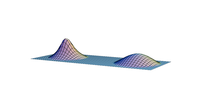
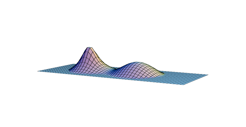
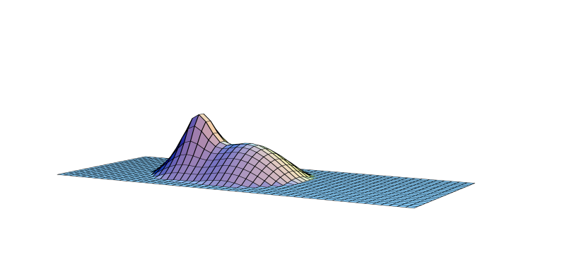
Figure 1: Shown are caloron profiles for $\omega=0.125$ (${\cal{T}}=1$), with $\rho=0.8,1.2,1.6$ (from left to right). This illustrates the growing separation of the two lumps with $\rho$. Once the constituents are separated, the lumps are spherically symmetric and do not change their shape upon further separation. Vertically is plotted the action density at $x_{0}=0$, on equal logarithmic scales for all profiles. They were cut off at an action density below $1/e^{2}$.

We will show below that in this limit they have unit, but opposite, magnetic charges and that the two lumps have spatial scales proportional to respectively $1/\bar{\omega}$ and $1/\omega$. This results in monopole masses of respectively $16\pi^{2}\bar{\omega}/{\cal{T}}$ and $16\pi^{2}\omega/{\cal{T}}$ for the two lumps. For $\omega=0$ or $\omega={\scriptstyle{{1\over 2}}}$, the second lump is absent and the solution is spherically symmetric. This is the Harrington-Shepard caloron [1], which was shown already by Rossi [10] to become the standard BPS monopole (after a singular gauge transformation) in the limit of large $\rho$.

3 Topological charge from monopoles

Apparently our solution provides an example of gauge fields with unit topological charge built out of monopole fields. We will argue this to be much more general than implied by our solution. Let us recall briefly some old arguments by Taubes [11]. Non-trivial ${SU(2)}$ monopole fields are classified by the winding number of maps from $S^{2}$ to $SU(2)/U(1)\!\sim\!S^{2}$, where ${U(1)}$ is the unbroken gauge group. We consider at this point configurations at a fixed time $t$, $\Psi=\{A_{\mu}(\vec{x})\}$. In the sector where the net winding vanishes, we study a one-parameter family of configurations, $\Psi_{t}=\{A_{\mu}(\vec{x},t)\}$ (the parameter can, but need not, be seen as the time $t$). When this configuration is made out of monopoles with opposite charges, in a suitable gauge the isospin orientations behave as shown in fig. 2, sufficiently far from the core of both monopoles. We rotate only one of the monopoles around the axis connecting them. The fields of two monopoles will in general no longer cancel when brought together, despite the fact that the long range abelian components do cancel. The non-contractible loop is now constructed by letting $t$ affect a full rotation.

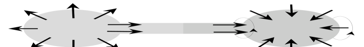
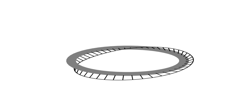
Figure 2: The non-contractible loop is constructed from two oppositely charged monopoles by rotating one of them, as indicated on the left. On the right is a closed monopole line, rotating its frame when completing the circle.

Taubes describes this by creating a monopole anti-monopole pair, bringing them far apart, rotating one of them over a full rotation and finally bringing them together to annihilate. The four dimensional configuration constructed this way is topologically non-trivial. Since an anti-monopole travelling forward in time is a monopole travelling backwards in time, we can describe this as a closed monopole line (or loop). It represents a topologically non-trivial configuration when the monopole makes a full rotation while moving along the closed monopole line (see fig. 2). The non-trivial topology is just the Hopf fibration. Here it is more natural to see $S^{1}$ as the base manifold and $S^{2}$ as the fibre, which rotates (twists) while moving along the circle formed by the closed monopole line. The only topological invariant available to characterise this homotopy type is precisely the Pontryagin index. The long range fields are abelian and cannot contribute to the topological charge. For our calorons the contribution to the topological charge density is indeed localised to the monopole core regions [6].

To inspect more closely the monopole content of our calorons we choose $\rho/{\cal{T}}$ large, such that the monopoles are well separated and static. For $\omega\bar{\omega}\neq 0$, outside the core of both monopole constituents, i.e. $r\bar{\omega}>1$ and $s\omega>1$, we have $\phi=\phi_{0}+{\cal{O}}(e^{-8\pi\,{\rm min}(s\omega,r\bar{\omega})})$ and $\tilde{\chi}=\tilde{\chi}_{0}\left(1+{\cal{O}}(e^{-8\pi\,{\rm min}(s\omega,r\bar{\omega})})\right)$, with

$$\phi_{0}=\frac{r+s+\pi\rho^{2}}{r+s-\pi\rho^{2}},\quad\tilde{\chi}_{0}=\frac{4\pi\rho^{2}}{(r+s+\pi\rho^{2})^{2}}\left\{re^{-4\pi r\bar{\omega}}e^{-2\pi ix_{0}}+se^{-4\pi s\omega}\right\}.$$ (8)

Substituting this in eq. (3) we find the solution to be time independent and abelian, up to exponential correction

$$A_{\mu}=\frac{i}{2}\tau_{3}\bar{\eta}_{\mu\nu}\partial_{\nu}\log\phi_{0},\quad E_{k}=\frac{i}{2}\tau_{3}\partial_{k}\partial_{3}\log\phi_{0},\quad B_{k}=\frac{i}{2}\tau_{3}\left(\partial_{k}\partial_{3}\log\phi_{0}-\delta_{k3}\partial_{j}^{2}\log\phi_{0}\right).$$ (9)

Self-duality, $\vec{E}=\vec{B}$, requires $\log\phi_{0}$ to be harmonic. Note that $\phi_{0}^{-1}$ vanishes on the line for $-2\pi\rho^{2}\omega\leq x_{3}\leq 2\pi\rho^{2}\bar{\omega}$ and $x_{1}=x_{2}=0$ and one finds $\partial_{j}^{2}\log\phi_{0}=-4\pi\delta(x_{1})\delta(x_{2})\chi_{\omega}(x_{3})$ (with $\chi_{\omega}(x_{3})=1$ where $\phi_{0}^{-1}=0$ and 0 elsewhere). The term $-\frac{i}{2}\tau_{3}\delta_{k3}\partial_{j}^{2}\log\phi_{0}$ in the expression for the magnetic field corresponds precisely to the Dirac string singularity, carrying the return flux. Ignoring this return flux, which in the full theory is absent, we find $\partial_{k}E_{k}=\partial_{k}B_{k}=\frac{i}{2}\tau_{3}\partial_{3}\partial_{j}^{2}\log\phi_{0}=2\pi i\tau_{3}(\delta_{3}(\vec{s})-\delta_{3}(\vec{r}))$. It remains to identify the rotation of one of the monopoles so as to guarantee the topologically non-trivial nature of the configuration. Inspecting the behaviour near the core region of the monopoles, gives the factorisation $\tilde{\chi}_{0}=\chi^{(1)}(r)+e^{-2\pi ix_{0}}\chi^{(2)}(s)$. While one of the monopoles has a static core, the other has a time dependent phase rotation - equivalent to a (gauge) rotation - precisely of the type required to form a non-contractible loop, as the phase makes a full rotation when closing by the periodic boundary conditions in the time direction.

Although interpreting $A_{0}$ as the Higgs field $\Phi$ allows one to introduce monopoles in pure gauge theory, there are some subtle differences, which form the basis of somewhat improper terminology. In the Higgs model one has $B_{i}\!=\!D_{i}\Phi$ and $E_{i}\!=\!-\partial_{0}A_{i}$ for the $A_{0}\!=\!0$ gauge. In pure gauge theory it makes, however, no sense to separate $D_{i}\Phi\!=\!D_{i}A_{0}$ from $\partial_{0}A_{i}$. Gauge invariance requires that they occur in the combination $F_{i0}\!=\!D_{i}A_{0}\!-\!\partial_{0}A_{i}$. The electric field is necessarily quantised as soon as we interpret $A_{0}$ as the Higgs field. It is thus misleading to talk about a dyon, for which the electric charge is not quantised [13]. Dyons in pure gauge theories can be obtained only after adding a $\theta$ term to the lagrangian [14]. It is interesting to note that in the Higgs model the construction of the non-contractible loop generates an electric charge due to the (gauge) rotation along the closed monopole line, when interpreting the loop parameter as time. The electric charge is proportional to the rate of rotation and can vary along the monopole line. However, integrated along a closed monopole line the charge is fixed and proportional to the number of rotations, which hence plays the role of a winding number. In pure gauge theory this winding can not be read off (for $\theta=0$) from the long range field components, but for both cases the fields in the core are responsible for the Pontryagin number.

4 Abelian projection, monopoles and instantons

Monopoles appear in the context of ’t Hooft’s abelian projection [12] as (gauge) singularities. In order to include the non-trivial topological charge, important for fermion zero modes, breaking of the axial $U(1)$ symmetry [8] and presumably for chiral symmetry breaking, as we have seen one needs to keep some information on the behaviour near the core of these monopoles. In lattice gauge theory abelian projection was implemented by the so-called maximal abelian gauge [15], in order to extract the monopole content of the theory. For a review see ref. [16]. Recently it was found that after abelian projection, instantons contain closed monopole lines [17]. In the light of Taubes’s construction this was to be expected, as emphasised in ref. [18]. What is minimally required, is a frame associated to each monopole, whose rotation is a topological invariant for closed monopole lines. Such closed monopole lines can shrink, but one will be left over with what represents an instanton. It would be interesting to build a hybrid model based on the instanton liquid [19] and monopoles [20].

To conclude, it is sensible to take the monopole content of instantons serious in the broader context sketched here. Our gauge invariant method of investigating the monopoles inside an instanton is somewhat destructive (but reversible). First we heat the instanton just a little. Then we add a non-trivial value of the Polyakov loop at infinity, without disturbing the instanton significantly (true for ${\cal{T}}$ sufficiently large). Now we have to squeeze (or heat) it hard. Out come the two constituent monopoles, in a direction determined by the choice we have made for the Polyakov loop at infinity (which does not change under heating). The new caloron solutions can be studied on the lattice by taking all links in the time direction, at the spatial boundary of the lattice, equal to $U_{0}=\exp(2\pi i\vec{\omega}\cdot\vec{\tau}/N_{0})$ (in lattice units ${\cal{T}}$ equals $N_{0}$). One can look for solutions using improved cooling [21] (to prevent calorons to disappear due to scaling violations). When interested in seeing the monopole constituents one may just as well take the time direction to be one lattice spacing ($N_{0}=1$). The lattice study of ref. [22] is interesting in this perspective.

References

- [1] B.J. Harrington and H.K. Shepard, Phys. Rev. D17 (1978) 2122; D18 (1978) 2990.
- [2] D.J. Gross, R.D. Pisarski and L.G. Yaffe, Rev. Mod. Phys. 53 (1983) 43.
- [3] G. ’t Hooft, as quoted in R. Jackiw, C. Nohl, C. Rebbi, Phys. Rev. D15 (1977) 1642.
- [4] M.F. Atiyah, N.J. Hitchin, V.G. Drinfeld, Yu. I. Manin, Phys. Lett. 65 A (1978) 185.
- [5] W. Nahm, Phys. Lett. 90B (1980) 413.
- [6] T.C. Kraan and P. van Baal, Phys. Lett. B428 (1998) 268 (hep-th/9802049); Periodic Instantons with non-trivial Holonomy, hep-th/9805168.
- [7] K. Lee and C. Lu, SU(2) calorons and magnetic monopoles, hep-th/9802108.
- [8] G. ’t Hooft, Phys. Rev. D14 (1976) 3432.
- [9] E.B. Bogomol’ny, Yad. Fiz. 24 (1976) 861; Sov. J. Nucl. 24 (1976) 449; M.K. Prasad and C.M. Sommerfield, Phys. Rev. Lett. 35 (1975) 760.
- [10] P. Rossi, Nucl. Phys. B149 (1979) 170.
- [11] C. Taubes, Morse theory and monopoles: topology in long range forces, in: Progress in gauge field theory, eds. G. ’t Hooft et al, (Plenum Press, New York, 1984) p. 563.
- [12] G. ’t Hooft, Nucl. Phys. B190[FS3] (1981) 455; Physica Scripta 25 (1982) 133.
- [13] B. Julia and A. Zee, Phys. Rev. D11 (1975) 2227.
- [14] E. Witten, Phys. Lett. 86B (1979) 283.
- [15] A.S. Kronfeld, G. Schierholz and U.J. Wiese, Nucl. Phys. B293 (1987) 461.
- [16] M. Polikarpov, Nucl.Phys. B(Proc. Suppl.)53 (1997) 134 (hep-lat/9609020).
- [17] M.N. Chernodub and F.V. Gubarev, JETP Lett. 62 (1995) 100 (hep-th/9506026); A. Hart and M. Teper, Phys.Lett. B372(1996) 261 (hep-lat/9511016); V. Bornyakov and G. Schierholz, Phys. Lett. B384(1996)190 (hep-lat/9605019).
- [18] P. van Baal, Nucl. Phys. B(Proc. Suppl.) 63A-C (1998) 126 (hep-lat/9709066).
- [19] T. Schäfer and E. Shuryak, Rev. Mod. Phys. 70 (1998) 323 (hep-ph/9610451).
- [20] J. Smit and A. van der Sijs, Nucl. Phys. B355 (1991) 603.
- [21] M. García Pérez, e.a., Nucl.Phys. B413(1994)535-553 (hep-lat/9309009).
- [22] M.L. Laursen and G. Schierholz, Z. Phys. C38 (1988) 501.