INLO-PUB-5/98

Abstract: We present the detailed derivation of the charge one periodic instantons - or calorons - with non-trivial holonomy for ${SU(2)}$. We use a suitable combination of the Nahm transformation and ADHM techniques. Our results rely on our ability to compute explicitly the relevant Green’s function in terms of which the solution can be conveniently expressed. We also discuss the properties of the moduli space, ${\rm I\kern-1.79993ptR}^{3}\times S^{1}\times$ Taub-NUT/$Z_{2}$ and its metric, relating the holonomy to the Taub-NUT mass parameter. We comment on the monopole constituent description of these calorons, how to retrieve topological charge in the context of abelian projection and possible applications to QCD.

1 Introduction

Instantons [1] and Bogomolny-Prasad-Sommerfield (BPS) monopoles [2] possess remarkable properties. They exist as exact solutions with arbitrary charges and with an action or energy, proportional to their integer charge. Therefore the multi-charge solutions can be seen as built from constituents of unit charge. Indeed, for BPS monopoles the absence of an interaction energy can be understood - for large separation - as a cancellation between the electro-magnetic and scalar interactions [3, 4].

Instantons are self-dual solutions with finite action. For non-compact manifolds, the solutions must approach vacua in the non-compact directions. Due to the topology of the base manifold, these vacua can be non-trivial and can give rise to extra parameters for these self-dual solutions. For periodic instantons on ${\rm I\kern-1.79993ptR}^{3}\times S^{1}$, also called calorons, the vacuum label is given by the eigenvalues of the Polyakov loop (holonomy) around $S^{1}$ at spatial infinity. Equivalently, one may consider this vacuum as the background field on which the solution is superposed. In this respect, they are very similar to monopole solutions in broken gauge theories, a non-trivial vacuum generally breaking the gauge symmetry.

Calorons can be seen to have as constituents BPS monopoles [5, 6] ($N$ for $SU(N)$), as follows from Nahm’s work [7]. The constituents are such that the net magnetic and electric charge of the caloron vanishes. Unlike for the ordinary multi-monopoles, the BPS constituents are hence of opposite charge, and thus have an attractive electro-magnetic interaction. Nevertheless, also here exact solutions exist with an action that does not depend on the parameters, though the solutions become static only for large separations. In order to have this non-trivial situation the Polyakov loop at spatial infinity has to be non-trivial, breaking the gauge invariance spontaneously. The eigenvalues of this Polyakov loop uniquely fix the masses of the constituent monopoles. Their separation - not surprisingly - is related to the scale parameter of the caloron solution.

In this paper we study periodic ${SU(2)}$ instantons with topological charge one and arbitrary holonomy [8]. Its purpose is to provide the necessary details for this construction. Central to our success in providing explicit and relatively simple new solutions is the construction of the relevant Green’s function. In the context of the Nahm transformation, introduced here as the Fourier transform of the Atiyah-Drinfeld-Hitchin-Manin (ADHM) data [1], this can be reduced to a quantum mechanical problem on the circle with a piecewise constant potential and well-defined delta function singularities related to the holonomy. We find compact expressions for the gauge field and action density of the solution and investigate the properties of the caloron. The moduli space is described in terms of the constituent monopoles, which in our approach appear as explicit lumps in the action density. Furthermore, we relate the constituent monopole nature of these instantons to work by Taubes in which he showed how to make gauge configurations with non-trivial topological charge out of monopole fields [9].

Independently, the recent work in ref. [10] has taken the constituent monopole description [5, 6, 7] as the starting point, suitably superposing two BPS monopole solutions to form a caloron solution.

Periodic instantons have been discussed first in the context of finite temperature field theory [11, 12], where the period (${\cal{T}}$) is the inverse temperature in euclidean field theory. A non-trivial value of the Polyakov loop will modify the vacuum fluctuations and thereby leads to a non-zero vacuum energy density as compared to a trivial Polyakov loop. It was on the basis of this observation that calorons with non-trivial holonomy were deemed irrelevant in the infinite volume limit [12]. It should be emphasised though, that the semi-classical one-instanton calculation is no longer considered a reliable approximation. At finite temperature $A_{0}$ can be seen to play the role of a Higgs field and in a strongly interacting environment one could envisage regions with this Higgs field pointing predominantly in a certain direction, and nevertheless having at infinity a trivial Higgs field. Given a finite density of periodic instantons, in an infinite volume solutions with non-trivial holonomy (in some average sense) may well have a role to play.

In our construction of the charge one caloron with non-trivial Polyakov loop, we pick a particular gauge. In the periodic gauge, the spatial components of the vacuum connection at infinity can be gauged to zero. The $A_{0}$ component can only be gauged to a constant, e.g.$A_{0}=2\pi i{\vec{\omega}}\cdot{\vec{\tau}}$ (with $\tau_{a}$ the Pauli matrices), when the total magnetic charge is vanishing. This connection has obviously a non-trivial Polyakov loop at infinity

$${\cal{P}}(\vec{x})=P\,\exp(\int_{0}^{\cal{T}}A_{0}(\vec{x},x_{0})dx_{0})\rightarrow e^{2\pi i\vec{\omega}\cdot\vec{\tau}}$$ (1)

($P$ stands for path-ordering). Alternatively, connections on ${\rm I\kern-1.79993ptR}^{3}\times S^{1}$ can be formulated by embedding them in ${\rm I\kern-1.79993ptR}^{4}$ and demanding periodicity modulo gauge transformations. Gauging with a non-periodic gauge transformation $g(\vec{x},x_{0})=e^{2\pi ix_{0}\vec{\omega}\cdot\vec{\tau}}$, starting from the periodic gauge with zero $A_{i}$ and constant $A_{0}=2\pi i\vec{\omega}\cdot\vec{\tau}$ at infinity, sets all gauge fields to zero at infinity. In that case we have

$$A_{\mu}(\vec{x},x_{0}+{\cal{T}})=e^{2\pi i\vec{\omega}\cdot\vec{\tau}}A_{\mu}(\vec{x},x_{0})e^{-2\pi i\vec{\omega}\cdot\vec{\tau}},$$ (2)

with ${\cal{T}}$ the period in the imaginary time direction, i.e. the inverse temperature. Clearly, $e^{2\pi i\vec{\omega}\cdot\vec{\tau}}\equiv g_{0}({\vec{x}})$ is the transition function or cocycle. Using the proper expression for the Polyakov loop along a path traversing the boundary between coordinate patches [13],

$${\cal{P}}(\vec{x})=P\,\exp(\int_{0}^{\cal{T}}A_{0}(\vec{x},x_{0})dx_{0})g_{0}(\vec{x}),$$ (3)

we find the same value for the holonomy in this gauge, the holonomy at infinity now solely being carried by the cocycle $g_{0}({\vec{x}})$. It is in this so-called “algebraic” gauge that we will calculate the generalised caloron solutions.

The charge $k$ instantons on ${\rm I\kern-1.79993ptR}^{4}$ are given by the ADHM construction [1]. The Nahm transformation forms a modification of this approach, initially introduced by Nahm to study BPS monopoles [14, 15]. Later developments culminated in the Nahm duality transformation on generalised tori, which forms a powerful tool for studying self-dual connections. Also caloron solutions can be treated along these lines [7]. The Nahm transformation is outlined in section 2. We summarise in section 3 the details of the ADHM formalism necessary for our construction of the caloron in section 4. We make it evident how the two approaches are related by Fourier transformation. By relying on the ADHM construction we profit from the vast knowledge on multi-instanton calculus within this formalism. Section 4 forms the calculational core of this paper, in which we derive the gauge potential and a particularly simple expression for the action density. The various properties and symmetries of the caloron are unraveled in section 5. In section 6 we describe the moduli space of the caloron. In section 7 we discuss the relation to Taubes’s work, abelian projection [16] and possible applications to QCD.

2 The Nahm transformation

We will consider a $U(n)$ bundle $E$ with self-dual gauge connection $A_{\mu}$ on a four manifold $M={\rm I\kern-1.79993ptR}^{4}/H$, with instanton number $k$. Here $H$ is a subgroup of translation symmetries under which the physics is invariant. When $H$ is a four dimensional lattice, $M$ will be the four torus [17]. Other four manifolds are obtained by taking appropriate limits [18]. We demand the gauge potential to be invariant modulo gauge transformations under the action of $H$.

An essential ingredient in Nahm’s construction [15] is to add a curvature free abelian connection, $-2\pi iz_{\mu}dx_{\mu}$, to the gauge field and to study the Weyl operator

$$D_{z}(A)=\sigma_{\mu}D^{\mu}_{z}(A),\quad D^{\dagger}_{z}(A)=-{\bar{\sigma}}_{\mu}D_{z}^{\mu}(A),\quad D^{\mu}_{z}(A)=\partial_{\mu}+A_{\mu}-2\pi iz_{\mu}.$$ (4)

$\sigma_{\mu}=(1_{2},i\vec{\tau})$ and ${\bar{\sigma}}_{\mu}=\sigma^{\dagger}_{\mu}=(1_{2},-i\vec{\tau})$ are unit quaternions. As compared to usual conventions [17, 18], we replaced $z$ by $-z$ to facilitate matching with the ADHM construction. When $A$ is without flat factors (WFF, meaning that the vector bundle $E$ does not split in $E^{\prime}\oplus L$ for any flat line bundle $L$), then $D_{z}(A)$ will have a trivial kernel [19]. For such gauge fields $G_{z}(x,y)=(D^{\dagger}_{z}(A)D_{z}(A))^{-1}$ is well-defined. The index theorem [20, 21] shows that there are $k$ normalisable zero modes of the Weyl operator $D^{\dagger}_{z}(A)$, for each value of $z\in\hat{M}={\rm I\kern-1.79993ptR}^{4}/\hat{H}$, $\hat{H}=\{z\in{\rm I\kern-1.79993ptR}^{4}|z\cdot y\in{\rm Z\!\!Z},\,\forall y\in H\}$, cf. ref. [18]. We can therefore define a $U(k)$ connection on the space $\hat{M}$,

$$\hat{A}^{ij}_{\mu}(z)=\int_{M}dx~{}\psi_{z}^{i\dagger}(x)\frac{\partial}{\partial z_{\mu}}\psi_{z}^{j}(x),$$ (5)

where $\psi^{i}_{z}(x),~{}i=1,\ldots,k$ form an orthonormal basis for the Nahm bundle $\hat{E}$ of fermionic zero modes. This is called the Nahm transformed connection.

The Weitzenböck identity [19] states

$$D^{\dagger}_{z}(A)D_{z}(A)=-(D_{z}^{\mu}(A)D_{z}^{\mu}(A)+{\scriptstyle{{1\over 2}}}\bar{\eta}_{\mu\nu}F^{\mu\nu}(x)).$$ (6)

where $\bar{\eta}_{\mu\nu}=\bar{\eta}^{a}_{\mu\nu}\sigma_{a}={\bar{\sigma}}_{[\mu}\sigma_{\nu]}$ is the anti-selfdual and $\eta_{\mu\nu}=\eta^{a}_{\mu\nu}\sigma_{a}=\sigma_{[\mu}{\bar{\sigma}}_{\nu]}$ the self-dual  ’t Hooft tensor [22] (note that in our conventions time is labeled by $x_{0}$ rather than $x_{4}$, and to conform with anti-selfduality of $\bar{\eta}$ we define $\epsilon_{1230}=1$). As $F$ is self-dual, the second term will vanish, and hence $D^{\dagger}_{z}(A)D_{z}(A)$ and $G_{z}(x,y)$ commute with the quaternions. This has profound consequences for the curvature associated to the Nahm connection. One finds [18]

$$\hat{F}_{\mu\nu}(z)=8\pi^{2}\int_{M\times M}dxdy\,\psi_{z}^{\dagger}(x)G_{z}(x,y)\eta_{\mu\nu}\psi_{z}(y)$$ (7)

$$\qquad+4\pi i\int_{\partial M\times M}dS_{\lambda}(x)\,dy\,\frac{\partial}{\partial z_{\left[\mu\right.}}\psi_{z}^{\dagger}(x)\sigma_{\lambda}\bar{\sigma}_{\left.\nu\right]}G_{z}(x,y)\psi_{z}(y),$$

where $\psi_{z}$ denotes the matrix with the zero modes $\psi^{i}_{z}$ as columns. Here we used that $G$ commutes with the quaternions. The first term is clearly self-dual. The boundary term shows possible deviations from self-duality, which occur at the points $z$ for which the zero modes do not decay exponentially in the non-compact directions. In these directions the connection necessarily approaches a vacuum for the action to be finite. These vacua are labeled by the eigenvalues of the Polyakov loops ${\cal{P}}_{i}=P\exp\int_{C_{i}}A_{\mu}dx_{\mu}$ along the circles $C_{i}$ corresponding to the compact directions. In the case that $e^{2\pi iz}$ becomes equal to one of these eigenvalues, the component of $A_{\mu}-2\pi iz_{\mu}$ along $C_{i}$ in eq. (4) will develop a zero eigenvalue when approaching infinity. This gives rise to a surviving boundary term in eq. (7) and as a result a deviation from self-duality, precisely for these specific points. As the deviations occur in single points, they will be expressible in delta functions. Hence, $\hat{F}_{\mu\nu}$ is self-dual almost everywhere. For the non-compact directions $\mu$, the $z_{\mu}$ dependence of $\psi_{z}(x)$ is a plane wave factor, and hence $\hat{A}$ is $z_{\mu}$ independent. Note that the $U(k)$ symmetry in the space of zero modes associated to $A$ is mapped onto a gauge symmetry for $\hat{A}$. On the other hand, gauge transformations on $A$ leave $\hat{A}$ unchanged.

For the four torus $T^{4}$ the boundary terms are absent and instantons are mapped onto instantons. It can be shown, using the family index theorem, that under this Nahm transformation a $U(n)$ connection with topological charge $k$ is mapped onto a $U(k)$ connection with topological charge $n$. The Nahm transformation on $T^{4}$ squares to the identity [17]. More explicitly, the dual Weyl operator $\hat{D}^{\dagger}_{x}(\hat{A})=-{\bar{\sigma}}_{\mu}(\hat{\partial}_{\mu}+\hat{A}_{\mu}-2\pi ix_{\mu})$ has $n$ zero modes

$$\hat{D}^{\dagger}_{x}(\hat{A})\hat{\psi}_{x}^{i}(z)=0,\quad i=1,\ldots,n$$ (8)

in terms of which the original connection $A_{\mu}(x)$ is reconstructed

$$A^{ij}_{\mu}(x)=\int_{\hat{M}}dz~{}\hat{\psi}^{\dagger i}_{x}(z)\frac{\partial}{\partial x_{\mu}}\hat{\psi}_{x}^{j}(z).$$ (9)

This suggests to use the Nahm transformation in the construction of self-dual connections on modified tori, in situations when one can explicitly find the dual connection $\hat{A}$. Generally one expects this to be feasible when the Nahm transformed bundle is simpler than the original, in particular when $\hat{M}$ is of lower dimension than $M$. Another simplification arises for the case of topological charge $k=1$, since in that case the Nahm connection $\hat{A}$ is abelian. Because of the boundary terms, the second Nahm transformation will have to be modified by properly handling the singularities. The extreme case is $M={\rm I\kern-1.79993ptR}^{4},~{}H=0$, where the dual manifold $\hat{M}$ is just a point and the pair formed by the dual Weyl operator and singularities reduce to matrices which precisely give the ADHM data [7, 18, 19, 23]. The Nahm transformation on ${\rm I\kern-1.79993ptR}^{4}/H$ encompasses the ADHM construction.

We will now consider the Nahm transformation for calorons (using the classical scale invariance of the self-duality equations, we can choose ${\cal{T}}=1$ such that $H={\rm Z\!\!Z}$) and monopoles in the BPS limit ($H={\rm I\kern-1.79993ptR}$). For the latter, $A_{0}$ is interpreted as the Higgs field. Thus we can unify these two cases by considering them as connections on ${\rm I\kern-1.79993ptR}^{3}\times S^{1}$. The connections for ${\rm I\kern-1.79993ptR}^{3}\times S^{1}$ are topologically classified according to their behaviour at the boundary, $S^{2}\times S^{1}$. We give a short summary of the classification presented in ref. [12].

For the action to be finite, it is necessary that the connections go to a vacuum at spatial infinity. Generally, gauge vacua are labeled by the conjugacy classes of representations of maps of the first homotopy group to the gauge group [19]. For $S^{2}\times S^{1}$, we can characterise each vacuum by a gauge equivalence class of an element of the gauge group. Using a gauge transformation, this element can be chosen diagonal. The vacuum at infinity is related to the holonomy along the $S^{1}$ (or Polyakov loop), eq. (1) in the periodic gauge. The difference of a closed Wilson loop evaluated along two curves $C$ and $C^{\prime}$ is related with the flux through the surface swept out by the curves interpolating between $C$ and $C^{\prime}$. Hence, at spatial infinity where the curvature vanishes, a small deformation of the path $C$ around which the holonomy is measured does not influence ${\cal{P}}({\vec{x}})$. Only the homotopy of $C$ is important, and the holonomy at spatial infinity is a topological invariant. Therefore, at spatial infinity the eigenvalues of ${\cal{P}}({\vec{x}})$ become constants

$${\cal{P}}({\vec{x}})\rightarrow V(\hat{x})\exp[2\pi i\,{\rm diag}(\mu_{1},\cdots,\mu_{n})]V^{-1}(\hat{x}),\quad\sum_{i}\mu_{i}=0,$$ (10)

and we have, up to an $\hat{x}$ dependent gauge transformation $V$,

$$A_{0}=2\pi i\,{\rm diag}(\mu_{1},\cdots,\mu_{n})-i\,{\rm diag}(k_{1},\cdots,k_{n})/2r+{\cal{O}}(r^{-2}),\quad\sum_{i}k_{i}=0.$$ (11)

The gauge transformation $V$ induces a map from $S^{2}$ to the factor group $G/H_{\infty}$, with $H_{\infty}$ the isotropy group of $\exp[2\pi i\,{\rm diag}(\mu_{1},\cdots,\mu_{n})]$. For $SU(n)$ these maps $V(\hat{x})\rightarrow SU(n)/H_{\infty}$ are classified according to the fundamental group of $H_{\infty}$. Generically, $H_{\infty}$ consists of several $U(1)$ and $SU(N),\,N>1$ subgroups. Each $U(1)$ gives rise to a monopole winding number, related to the integers $k_{i}$.

The other topological quantum number is related to the homotopy class of the map $\partial M=S^{2}\times S^{1}\rightarrow SU(N)$ which occurs in the gauge transformation connecting the behaviour near the origin to that at infinity, which is classified by the instanton number $k\in\pi_{3}(SU(n))={\rm Z\!\!Z}$. Gauge connections on ${\rm I\kern-1.79993ptR}^{3}\times S^{1}$ are therefore classified by $\mu_{i}$, $k_{i}$ and $k$. We will consider the situation where the net magnetic charges of the solution vanish, $k_{i}=0$. For non-zero $k_{i}$ the situation is as for the (static) BPS monopoles, where the dimension of the space of fermionic zero modes depends on $z$. The jumps occur exactly where $z=\mu_{i}$, according to the Callias-Bott-Seeley theorem [21] (the situation of non-maximal symmetry breaking, where two or more $\mu_{i}$ coincide, is more involved).

For a periodic instanton with no net magnetic charges the fermionic zero modes are associated to the instanton winding number $k$ in the usual way. Hence, the rank of the Nahm transformed gauge potential is $k$ and as the ${\vec{z}}$ dependence of the fermionic zero modes is that of a plane wave, $\psi_{z_{0},\vec{z}}(x)=e^{2\pi i\vec{x}\cdot\vec{z}}\psi_{z_{0},\vec{0}}(x)$, one finds $\hat{A}$ to be ${\vec{z}}$ independent. The dual space $\hat{M}$ is an interval on the real line, with coordinate $z_{0}\equiv z$. For monopoles, this interval is $[\mu_{1},\mu_{n}]$ (when we order $\mu_{i}\leq\mu_{i+1}$). For calorons $z$ is the coordinate on the dual circle and $\hat{A}$ is periodic. The Nahm transformed curvature reduces to

$$\hat{F}_{0i}(z)={\frac{d}{dz}}\hat{A}_{i}+[\hat{A}_{0},\hat{A}_{i}],\quad\hat{F}_{ij}(z)=[\hat{A}_{i},\hat{A}_{j}].$$ (12)

Using the self-duality of the first term in eq. (7), and the fact that the second term of this equation is zero almost everywhere, except for possible delta function singularities at $z=\mu_{i}$ one finds

$${\frac{d}{dz}}\hat{A}_{i}+[\hat{A}_{0},\hat{A}_{i}]+{\scriptstyle{{1\over 2}}}\epsilon_{ijk}[\hat{A}_{j},\hat{A}_{k}]=\sum_{i}\alpha_{i}\delta(z-\mu_{i}).$$ (13)

These are the celebrated Nahm equations. Any $\hat{A}_{\mu}(z)$ obeying the Nahm equation of the right dimensionalities and singularity structure gives rise to a BPS monopole or caloron. For monopoles this is generally proven using twistor methods [15, 24], but for ${SU(2)}$ monopoles there exist direct proofs of the equivalence, without an intermediate twistor step [25]. For calorons the construction was formulated in ref. [7] and the twistor method for these periodic instantons was given in ref. [5], but a relation with existence theorems or a full circle reciprocity proof as it exists for monopoles and for instantons on ${\rm I\kern-1.79993ptR}^{4}$ and $T^{4}$ seems not to be present.

For the $k=1$ ${SU(2)}$ caloron, $\hat{A}_{\mu}$ is a ${U(1)}$ connection on the circle with 2 singularities corresponding to the holonomy. Note that here $\mu_{2}=-\mu_{1}=\omega$, with $\omega\equiv|\vec{\omega}|\in[0,{\scriptstyle{{1\over 2}}}]$. The magnetic components of $\hat{F}$ vanish and hence non-zero values and singularities are only assumed by the electric components $\hat{F}_{0i}$. By the Nahm equations $\hat{A}$ is forced to be piecewise constant. We will give the explicit ADHM construction for these calorons and show among other things that all aspects suggested in ref. [7] arise automatically.

3 The ADHM construction

We first summarise the ADHM construction [1, 26] for charge $k$ ${SU(2)}$ instantons on ${\rm I\kern-1.79993ptR}^{4}$. Generalisation to higher groups is well-known but will detract one from the simplicity of our construction. The ADHM data consist of a quaternionic row vector $\lambda=(\lambda_{1},\cdots,\lambda_{k})$ and a quaternionic, symmetric $k\times k$ matrix $B$ ($\lambda_{m}\equiv\lambda^{\mu}_{m}\sigma_{\mu}$ and $B_{m,n}\equiv B^{\mu}_{m,n}\sigma_{\mu}$, with $\lambda_{m}^{\mu}\in{\rm I\kern-1.79993ptR}$ and $B_{m,n}^{\mu}=B_{n,m}^{\mu}\in{\rm I\kern-1.79993ptR}$). These objects are comprised in

$$\Delta(x)=\left(\!\!\begin{array}[]{c}\lambda\\ B-x\end{array}\!\!\right).$$ (14)

Here, the quaternion $x\equiv x_{\mu}\sigma_{\mu}$ denotes the position variable and a $k\times k$ unit matrix is implicit in our notation. For later use, we define $\Delta\equiv\Delta(x=0)$. The ADHM gauge potential is given by

$$A_{\mu}(x)=v^{\dagger}(x)\partial_{\mu}v(x),$$ (15)

where $v(x)$ is a $(k+1)$ dimensional quaternionic vector, the normalised solution to

$$\Delta^{\dagger}(x)v(x)=0.$$ (16)

For this construction to give a self-dual potential $A_{\mu}$, $\Delta(x)$ has to satisfy the ADHM constraints. These demand that $\Delta^{\dagger}(x)\Delta(x)$ be real quaternionic (i.e. commutes with the quaternions) and invertible. It is sufficient for this to hold at $x=0$, i.e., $\Delta^{\dagger}\Delta=B^{\dagger}B+\lambda^{\dagger}\lambda$ must be real quaternionic and invertible. Furthermore $(B-x)$ should have a trivial kernel, except for $k$ values of $x$, where $v(x)$ and, as a consequence, $A_{\mu}(x)$ are singular. This can be shown to be a gauge singularity and implements the non-triviality of the bundle and reflects the topological nature of these solutions.

This construction gives all instantons on ${\rm I\kern-1.79993ptR}^{4}$. The following transformations

$$\lambda\rightarrow\lambda T^{-1},~{}B\rightarrow TBT^{-1},~{}T\in O(k),$$ (17)

$$\lambda\rightarrow g\lambda,\quad g\in{SU(2)},$$

both leave the quadratic ADHM constraint untouched. The first does not change $A_{\mu}(x)$, whereas the second induces a global gauge transformation. Local gauge transformations arise from the $U(2)$ symmetry $v(x)\rightarrow v(x)g(x)$ in the solution space of eq. (16). One must divide out these symmetries in order to obtain all gauge inequivalent solutions. This reduces the dimension of the space of gauge inequivalent solutions to $8k(-3)$, depending on whether or not the global gauge degrees of freedom are included as moduli. Considering the $g$ as moduli, the moduli space is an $8k$ dimensional hyperKähler manifold [19].

Many aspects featuring in the construction above have their counterparts in the Nahm transformation. The reality constraint is similar to the vanishing of the imaginary quaternions in the Weitzenböck formula, which leads to the self-duality of the Nahm connection. The symmetries in the ADHM construction can be traced back to the triviality of the gauge action in the Nahm transformation and the unitary symmetry of the fermionic zero modes. We define two matrix inverses, the analogues of the Green’s functions,

$$f_{x}=(\Delta(x)^{\dagger}\Delta(x))^{-1}\in{\rm I\kern-1.79993ptR}^{k\times k},\quad G_{x}=((B-x)^{\dagger}(B-x))^{-1}\in{\rm I\!H}^{k\times k},$$ (18)

and a scalar function

$$\phi(x)=1+\lambda G_{x}\lambda^{\dagger}.$$ (19)

These Green’s functions $f_{x}$ and $G_{x}$ are related, as can be seen from the expansion of $f_{x}$ in terms of $G_{x}$,

$$f_{x}=(G_{x}^{-1}+\lambda^{\dagger}\lambda)^{-1}=G_{x}-G_{x}\lambda^{\dagger}\sum_{n=0}^{\infty}(-\lambda G_{x}\lambda^{\dagger})^{n}\lambda G_{x}=G_{x}-\phi^{-1}(x)G_{x}\lambda^{\dagger}\lambda G_{x},$$ (20)

Acting on eq. (20) with $\lambda^{\dagger}$ on the right and/or with $\lambda$ on the left, yields

$$G_{x}\lambda^{\dagger}=\phi(x)f_{x}\lambda^{\dagger},\quad\phi(x)=(1-\lambda f_{x}\lambda^{\dagger})^{-1}.$$ (21)

To solve for $v(x)$ in eq. (16), we introduce (a matrix of spinors) $u(x)$, and obtain

$$v(x)=\phi^{-{\scriptstyle{{1\over 2}}}}(x)\left(\!\!\begin{array}[]{c}-1\\ u(x)\end{array}\!\!\right),\quad u(x)=(B^{\dagger}-x^{\dagger})^{-1}\lambda^{\dagger},$$ (22)

where $\phi(x)=1+\lambda G_{x}\lambda^{\dagger}=1+u^{\dagger}(x)u(x)$ accounts for the normalisation of $v(x)$. In terms of these quantities, the gauge potential reads

$$A_{\mu}(x)={\scriptstyle{{1\over 2}}}\phi^{-1}(x)(u^{\dagger}(x)\partial_{\mu}u(x)-\partial_{\mu}u^{\dagger}(x)u(x)).$$ (23)

To show that the connection is indeed self-dual is best seen from using $F=dA+A\wedge A$, where $A=A_{\mu}dx_{\mu}$ and $F={\scriptstyle{{1\over 2}}}F_{\mu\nu}dx_{\mu}\wedge dx_{\nu}$. With $A=v^{\dagger}(x)dv(x)$ one finds

$$F=dv^{\dagger}(x)\wedge dv(x)-dv^{\dagger}(x)v(x)\wedge v^{\dagger}(x)dv(x)=dv^{\dagger}(x)(1-v(x)\!\otimes\!v^{\dagger}(x))dv(x).$$ (24)

As $1-v(x)\!\otimes\!v^{\dagger}(x)$ is the projection on the orthogonal complement of the kernel of $\Delta^{\dagger}(x)$ (since $\Delta^{\dagger}(x)v(x)=0$), we can use that $1-v(x)\otimes v^{\dagger}(x)=\Delta(x)f_{x}\Delta^{\dagger}(x)$. Substituting this in the expression for $F$ and using that $\Delta^{\dagger}(x)dv(x)=-dx_{\mu}\frac{\partial\Delta^{\dagger}(x)}{\partial x_{\mu}}v(x)=dx^{\dagger}(b^{\dagger}v(x))$ ($dx\equiv\sigma_{\mu}dx_{\mu}$, $b^{\dagger}v(x)\equiv\phi^{-{\scriptstyle{{1\over 2}}}}(x)u(x)$), we find [26]

$$F=(v^{\dagger}(x)b)dx\wedge f_{x}dx^{\dagger}(b^{\dagger}v(x)).$$ (25)

The crucial observation is now that the quadratic ADHM constraint implies that $f_{x}$ commutes with the quaternions and that $dx\wedge dx^{\dagger}=\eta_{\mu\nu}dx_{\mu}\wedge dx_{\nu}$, much like in the Nahm transformation where the Weitzenböck identity, eq. (6), guarantees that $D_{z}^{\dagger}(A)D_{z}(A)$ commutes with the quaternions. We thus find [23]

$$F_{\mu\nu}(x)=2\phi^{-1}(x)u^{\dagger}(x)\eta_{\mu\nu}f_{x}u(x),$$ (26)

which is self-dual due to the self-duality of $\eta_{\mu\nu}=\sigma_{[\mu}{\bar{\sigma}}_{\nu]}$.

In the case at hand, eq. (23) is of little practical use as it stands. We therefore rearrange it such that we can express $A_{\mu}$ in terms of evaluations of the Green’s function $f_{x}$. Using $\partial_{\mu}(B^{\dagger}-x^{\dagger})^{-1}=(B^{\dagger}-x^{\dagger})^{-1}{\bar{\sigma}}_{\mu}(B^{\dagger}-x^{\dagger})^{-1}=(B-x)G_{x}{\bar{\sigma}}_{\mu}(B-x)G_{x}$, we get

$$A_{\mu}(x)=\phi^{-1}(x)~{}\lambda G_{x}{\bar{\eta}}_{\mu\nu}(B-x)_{\nu}G_{x}\lambda^{\dagger}.$$ (27)

We substitute $G_{x}\lambda^{\dagger}=\phi(x)f_{x}\lambda^{\dagger}$, eq. (21), and noting that

$$\partial_{\nu}f_{x}^{-1}=\partial_{\nu}G_{x}^{-1}=-2(B-x)_{\nu},\quad(\partial_{\mu}f_{x}^{-1})f_{x}=-f_{x}^{-1}\partial_{\mu}f_{x},$$ (28)

we arrive at the following compact result for the gauge potential (see also ref. [27])

$$A_{\mu}(x)={\scriptstyle{{1\over 2}}}\phi(x)\partial_{\nu}\left(\lambda{\bar{\eta}}_{\mu\nu}f_{x}\lambda^{\dagger}\right),$$ (29)

using once again that $f_{x}$ commutes with the quaternions. When ${\bar{\eta}}_{\mu\nu}$ is moved through $\lambda$, one finds an expression for $A_{\mu}$ in terms of (derivatives of) “expectation values” of the Green’s function $f_{x}$.

$$A_{\mu}(x)={\scriptstyle{{1\over 2}}}\phi(x)\sigma_{\alpha}{\bar{\eta}}_{\mu\nu}\bar{\sigma}_{\beta}\partial_{\nu}\phi_{\alpha\beta},$$ (30)

where

$$\phi_{\alpha\beta}(x)=\phi_{\beta\alpha}(x)=(\lambda_{\alpha}f_{x}\lambda_{\beta}^{t}).$$ (31)

At this point we can make contact with the well-known ’t Hooft ansatz [28]. This forms a subclass of the ADHM construction with $\lambda$ real ($\lambda_{m}=\sigma_{0}\rho_{m}$) and $B_{m,n}=\delta_{m,n}y_{m}$ diagonal, corresponding to $k$ instantons with scales $\rho_{m}$ at positions $y_{m}$. This $5k$ dimensional family trivially satisfies the ADHM constraints. In this simpler situation the gauge potential can be written even in terms of a single scalar potential $\phi(x)=1+\sum_{k}\rho_{k}^{2}/|x-y_{k}|^{2}$ as $A_{\mu}(x)={\scriptstyle{{1\over 2}}}{\bar{\eta}}_{\mu\nu}\partial_{\nu}\log\phi(x)$, since $\phi_{00}(x)=1-\phi^{-1}(x)$.

For the action density, the following expression can be found in the literature [29, 23]

$${\rm tr}F^{2}_{\mu\nu}(x)=-\partial^{2}_{\mu}\partial^{2}_{\nu}\log\det f_{x}.$$ (32)

This expression is regular everywhere. We can rewrite eq. (32) using eq. (20) and eq. (28) as

$${\rm tr}F^{2}_{\mu\nu}(x)=-{\scriptstyle{{1\over 2}}}\partial^{2}_{\mu}\partial^{2}_{\nu}\log\det G_{x}+\partial^{2}_{\mu}\partial^{2}_{\nu}\log\phi(x).$$ (33)

The factor ${\scriptstyle{{1\over 2}}}$ is due to $G_{x}$ being considered as a quaternionic and $f_{x}$ as a real $k\times k$ matrix. For the ’t Hooft ansatz, $\partial^{2}_{\mu}\log\det G_{x}$ vanishes, except for delta functions at $x=y_{k}$, and we retrieve the known result [28], ${\rm tr}F^{2}_{\mu\nu}=\partial^{2}_{\mu}\partial^{2}_{\nu}\log\phi(x)$, which is indeed singular at these points (inadvertently in sect. 2 of ref. [8], ${\rm tr}F_{\mu\nu}^{2}$ was given with the wrong sign).

4 The construction of the caloron

In this section we describe the ADHM construction of caloron solutions with non-trivial holonomy. This will be a two-step process. Crucial will be the interpretation of the ADHM data as the Fourier coefficients of the Weyl operator in the Nahm transformation. In our strategy, we build the caloron as an infinite, periodic (gauge-twisted) chain of instantons. It will be shown how we can realise this within the ADHM construction, by solving the quadratic constraint on the ADHM data. To find $A_{\mu}(x)$ we use again a Fourier transform to construct $\hat{f}_{x}(z,z^{\prime})$, the Green’s function of an ordinary second order differential equation, which allows for the determination of $\phi_{\alpha\beta}(x)=(\lambda_{\alpha}f_{x}\lambda_{\beta}^{t})$, see eq. (30).

The boundary conditions $A_{\mu}(x+{\cal{T}})=e^{2\pi i\vec{\omega}\cdot\vec{\tau}}A_{\mu}(x)e^{-2\pi i\vec{\omega}\cdot\vec{\tau}}$ are satisfied when

$$u_{k}(x+{\cal{T}})=u_{k-1}(x)\exp(-2\pi i\vec{\omega}\cdot\vec{\tau}),$$ (34)

as is seen from eq. (23). This is implemented by the periodicity constraints

$$\lambda_{k+1}=e^{2\pi i\vec{\omega}\cdot\vec{\tau}}\lambda_{k},\quad B(x+{\cal{T}})_{m,n}=B(x)_{m-1,n-1},$$ (35)

where $B(x)=B-x$. It now follows that

$$B_{m+1,n+1}=B_{m,n}+{\cal{T}}\delta_{m,n},$$ (36)

the inhomogeneous part of which is solved by having $\ldots,-2{\cal{T}},-{\cal{T}},0,{\cal{T}},2{\cal{T}},\ldots$ on the diagonal of $B$. We still have to determine the remainder of $B$, called $\hat{A}$ (anticipating its interpretation as Nahm connection), that contains its off-diagonal entries. In order to satisfy eq. (35), $\hat{A}$ has to be of a convolutive type $\hat{A}_{m,n}=\hat{A}_{m-n}$, such that

$$\lambda_{k}=e^{2\pi ik\vec{\omega}\cdot\vec{\tau}}\zeta,\quad\zeta=\rho q,\quad B_{m,n}={\cal{T}}m\delta_{m,n}+\hat{A}_{m-n}.$$ (37)

Here $\zeta$ is an arbitrary quaternion. Its length $\rho=|\zeta|$ is the scale parameter of the caloron. The ${SU(2)}$ element $q=\zeta/\rho$ describes its combined spatial and gauge orientation. The diagonal of $\hat{A}_{m,n}$ is necessarily constant, $\hat{A}^{\rm diag}_{m,n}\equiv\xi$, and plays the role of the position of the caloron. The ADHM data can now be readily interpreted as describing a periodic array of instantons, with temporal spacing ${\cal{T}}$ and relative gauge orientation $e^{2\pi i\vec{\omega}\cdot\vec{\tau}}$, with off-diagonal terms to account for the non-linear constraints. To simplify notations, we use the scale invariance of the self-duality equations to set ${\cal{T}}=1$. On dimensional grounds one can easily reinstate the proper ${\cal{T}}$ dependence when required.

When we perform the Fourier transformation, $B$ will be transformed into a Weyl operator, $\lambda$ and $\lambda^{\dagger}\lambda$ into delta function singularities and $u(x)$ into a spinor (to be more precise a $2\times 2$ matrix with as columns $\hat{\psi}_{x}^{i}$, cmp. sect. 2):

$$\sum_{m,n}B_{m,n}(x)e^{2\pi i(mz-nz^{\prime})}=\frac{\delta(z-z^{\prime})}{2\pi i}\hat{D}_{x}(z^{\prime}),\quad\hat{D}_{x}(z)=\sigma_{\mu}D_{x}^{\mu}(z)={\frac{d}{dz}}+\hat{A}(z)-2\pi ix,$$

$$\sum_{m}\lambda_{m}e^{2\pi imz}=\hat{\lambda}(z),\quad\hat{\lambda}(z)=(P_{+}\delta(z-\omega)+P_{-}\delta(z+\omega))\zeta,\quad P_{\pm}={\scriptstyle{{1\over 2}}}(1\pm\hat{\omega}\cdot\vec{\tau}),$$

$$\sum_{m}\lambda^{\dagger}_{m}\lambda_{n}e^{2\pi i(mz-nz^{\prime})}=\hat{\lambda}^{\dagger}(z^{\prime})\hat{\lambda}(z)=\delta(z-z^{\prime})\hat{\Lambda}(z),\quad\hat{\Lambda}(z)=\bar{\zeta}\hat{\lambda}(z)=\hat{\lambda}^{\dagger}(z)\zeta,$$

$$\sum_{m}u_{m}(x)e^{2\pi imz}=\hat{\psi}_{x}(z).$$ (38)

All these objects are defined on $S^{1}$, or more appropriately from the Nahm perspective, on ${\rm I\kern-1.79993ptR}^{4}/\hat{H}={\rm I\kern-1.79993ptR}^{4}/({\rm I\kern-1.79993ptR}^{3}\times{\rm Z\!\!Z})$. Note that $\hat{A}(z)=\sigma_{\mu}\hat{A}_{\mu}(z)=2\pi i\sum_{m}\exp(2\pi imz)\hat{A}_{m}$, such that from the symmetry of $\hat{A}_{m,n}$ (implying $\hat{A}_{m}=\hat{A}_{-m}$) it follows that $\hat{A}_{\mu}(z)$ is imaginary such that the differential operator $\hat{D}_{x}(x)$ is exactly the dual Weyl operator $\hat{D}_{x}(\hat{A})$ introduced in sect. 2 (to agree with the notation there we have - unlike in ref. [8] - included a factor $2\pi i$ in our definitions). Combining these features, we can interpret the Fourier transform of the ADHM construction as the inverse (or second) Nahm transformation.

The symmetries in the ADHM construction for periodic instantons lead to a $U(1)$ gauge symmetry for $\hat{A}_{\mu}(z)$. In order for eq. (17) to preserve the periodicity constraint eq. (35), $T$ has to be of a convolutive type, $T_{m,n}=T_{m-n}$. Defining the periodic function $\hat{g}(z)=\sum_{m}\exp(2\pi imz)T_{m}$ and using the fact that $T$ is orthogonal ($T^{-1}_{m,n}=T_{n-m}$ and $\sum_{k}T_{k+n}T_{k}=\delta_{n,0}$), one concludes that $\hat{g}(z)\in U(1)$. A gauge transformation with $\hat{g}(z)$ leaves $\hat{A}_{i}(z)$ invariant and transforms $\hat{A}_{0}(z)$ to $\hat{A}_{0}(z)-d\log\hat{g}(z)/dz$. Note that $\hat{A}_{0}(z)$ can be gauged away, apart from a constant (as the Polyakov loop is gauge invariant). Hence we may choose $\hat{A}_{0}(z)=2\pi i\xi_{0}$.

To implement the quadratic ADHM constraint after Fourier transformation we note that any complex $2\times 2$ matrix $W$ can be decomposed as $W=W_{\mu}\sigma_{\mu}$ and that $[W,\sigma_{\mu}]=0$ can be implemented by requiring ${\Im m}W=0$, provided we define ${\Im m}W\equiv{\scriptstyle{{1\over 2}}}[W-\tau_{2}W^{t}\tau_{2}]$. Also note that ${\Re e}W\equiv{\scriptstyle{{1\over 2}}}[W+\tau_{2}W^{t}\tau_{2}]={\scriptstyle{{1\over 2}}}{\rm tr}~{}W=W_{0}$. Thus, the quadratic ADHM constraint can be formulated as

$${\Im m}(\hat{D}_{x}^{\dagger}(z)\hat{D}_{x}(z)+4\pi^{2}\hat{\Lambda}(z))=0.$$ (39)

From the Weitzenböck formula $\hat{D}^{\dagger}_{x}(z)\hat{D}_{x}(z)=-(\hat{D}_{x}^{\mu}(z)\hat{D}_{x}^{\mu}(z)+{\scriptstyle{{1\over 2}}}{\bar{\eta}}_{\mu\nu}\hat{F}_{\mu\nu})$ (cmp. eq. (6)) we find

$${\frac{d}{dz}}\hat{A}(z) = {\scriptstyle{{1\over 2}}}{\bar{\eta}}_{\mu\nu}\hat{F}_{\mu\nu}(z)=-{\Im m}\hat{D}^{\dagger}_{x}(z)\hat{D}_{x}(z)=4\pi^{2}{\Im m}\hat{\Lambda}(z)$$ (40)

$$= 2\pi^{2}(\bar{\zeta}\hat{\omega}\cdot\vec{\tau}\zeta)(\delta(z-\omega)-\delta(z+\omega)),$$

using eq. (39) and $\hat{F}_{ij}(z)=0$. This leads to [30]

$$\hat{A}(z)=\sigma_{\mu}\hat{A}_{\mu}(z)=2\pi i[\xi+\pi(\bar{\zeta}\hat{\omega}\cdot\vec{\sigma}\zeta)\Theta_{\omega}(z)],$$ (41)

where (see fig. 1)

$$\Theta_{\omega}(z)=(\chi_{[-\omega,\omega]}(z)-2\omega).$$ (42)

Here $\chi_{[a,b]}(z)=1$ if $z\in[a,b]$ and 0 elsewhere, properly defined on the circle. We have arranged $2\pi i\xi=\int dz~{}\hat{A}(z)$, such that $B(x)$ has a single zero mode for $x=\xi$, to agree with the interpretation of $\xi$ as the position (centre of mass) of the caloron. Fourier transforming back, we retrieve the matrix representation of $B(x)$

$$B_{m,n}(x)=(m+\xi-x)\delta_{m,n}+\bar{\zeta}\hat{\omega}\cdot\vec{\sigma}\zeta\frac{\sin(2\pi(m-n)\omega)}{m-n}(1-\delta_{m,n}).$$ (43)

The moduli space is thus parametrised by the caloron position $\xi$ and by its scale and orientation $\zeta=\rho q$, with $\xi_{0}\in S^{1}$, $\vec{\xi}\in{\rm I\kern-1.79993ptR}^{3}$, $\rho\in{\rm I\kern-1.79993ptR}^{+}$ and $q\in{SU(2)}$.

Figure 1: The function $\Theta_{\omega}(z)$.

We end this first step in the construction by noting that the delta function singularities arise precisely as predicted by the general properties of the Nahm transformation, discussed in section 2 and that $\hat{A}(z)$ constructed in this section solves the Nahm equations, whereby we have found all self-dual solutions for ${\rm I\kern-1.79993ptR}^{3}\times S^{1}$.

For the second step we have to find the Green’s function $f_{x}$. For further notational simplification we absorb $\xi$ by a translation (we have already used the scale invariance to fix ${\cal{T}}=1$) such that after a Fourier transformation the definition of $f_{x}$, eq. (18), can be cast into a differential equation for $\hat{f}_{x}(z,z^{\prime})\equiv\sum_{n,m}f_{x}^{m,n}e^{2\pi i(mz-nz^{\prime})}$

$$\left\{\!\!\left(\!\frac{1}{2\pi i}{\frac{d}{dz}}\!-\!x_{0}\right)^{\!\!2}\!\!+\!s^{2}\chi_{[-\omega,\omega]}(z)\!+\!r^{2}\chi_{[\omega,1-\omega]}(z)\!+\!\frac{\rho^{2}}{2}(\delta(z\!\!-\!\!\omega)\!+\!\delta(z\!\!+\!\!\omega))\!\right\}\!\!\hat{f}_{x}(z,z^{\prime})=\delta(z-z^{\prime}).$$ (44)

Here, the radii $r$ and $s$ are given by

$$r^{2}={\scriptstyle{{1\over 2}}}{\rm tr}(\vec{x}\cdot\vec{\tau}+2\pi\omega\rho^{2}\bar{q}\hat{\omega}\cdot\vec{\tau}q)^{2},\quad s^{2}={\scriptstyle{{1\over 2}}}{\rm tr}(\vec{x}\cdot\vec{\tau}-2\pi\bar{\omega}\rho^{2}\bar{q}\hat{\omega}\cdot\vec{\tau}q)^{2},\quad(\bar{\omega}={\scriptstyle{{1\over 2}}}-\omega),$$ (45)

and can be interpreted as the respective centre of mass radii of the two constituent monopoles of the caloron. Note that $\bar{q}\hat{\omega}\cdot\vec{\tau}q$ shows how global gauge rotations are to be correlated to spatial rotations so as to keep the holonomy unchanged. We will come back to this in the next section. The symmetries of $\Delta^{\dagger}(x)\Delta(x)$ imply for the Green’s function $\hat{f}_{x}(z,z^{\prime})$ the following relations,

$$\hat{f}_{x}(z,z^{\prime})=\hat{f}_{x}(-z,-z^{\prime})^{*}=\hat{f}_{x}(-z^{\prime},-z)=\hat{f}_{x}(z^{\prime},z)^{*}.$$ (46)

In particular we have $\hat{f}_{x}(\omega,\omega)=\hat{f}_{x}(-\omega,-\omega)\in{\rm I\kern-1.79993ptR}$ and $\hat{f}_{x}(\omega,-\omega)=\hat{f}_{x}(-\omega,\omega)^{*}$. The Green’s function is that of ordinary quantum mechanics on a circle with a piecewise constant potential and delta function singularities of strength ${\scriptstyle{{1\over 2}}}\rho^{2}$ at the jumping points $z=\pm\omega$. It can thus be constructed in the usual straightforward (but tedious) method of matching the value of the Green’s function and its derivative (up to the appropriate jumps) at $z=\pm\omega$ and $z=z^{\prime}$. The result reads

$$\hat{f}_{x}(z,z^{\prime})=\chi_{[-\omega,\omega]}(z^{\prime})\left(\chi_{[-\omega,\omega]}(z)\hat{f}^{d}_{x}(z,z^{\prime},r,s,\omega)+\chi_{[\omega,1-\omega]}(z)\hat{f}^{o}_{x}(z,z^{\prime},r,s,\omega)\right)+$$

$$\quad~{}\,\chi_{[\omega,1-\omega]}(z^{\prime})\left(\chi_{[\omega,1-\omega]}(z)\hat{f}^{d}_{x}(z\!-\!{\scriptstyle{{1\over 2}}},z^{\prime}\!-\!{\scriptstyle{{1\over 2}}},s,r,\bar{\omega})+\chi_{[-\omega,\omega]}(z)\hat{f}^{o}_{x}(z^{\prime},z,r,s,\omega)^{*}\right).$$ (47)

In the following the diagonal component $\hat{f}^{d}_{x}(z,z^{\prime})$ is only defined strictly for $z,z^{\prime}\in[-\omega,\omega]$ and the off-diagonal component $\hat{f}^{o}_{x}(z,z^{\prime})$ only for $z\in[\omega,1-\omega]$ and $z^{\prime}\in[-\omega,\omega]$. For $z$ or $z^{\prime}$ outside of these intervals, one first has to map back to the interval $[-\omega,1-\omega]$, using periodicity.

$$\hskip-19.91692pt\hat{f}^{d}_{x}(z,z^{\prime},r,s,\omega)=e^{2\pi ix_{0}(z-z^{\prime})}\pi(rs\psi)^{-1}\Big{\{}e^{-2\pi ix_{0}{\rm sign}(z-z^{\prime})}r\sinh(2\pi s|z\!-\!z^{\prime}|)$$

$$\qquad\qquad~{}~{}-s^{-1}\cosh(2\pi s(z\!+\!z^{\prime}))\left[\pi\rho^{2}r\cosh(4\pi r\bar{\omega})+{\scriptstyle{{1\over 2}}}(r^{2}\!-\!s^{2}\!+\!\pi^{2}\rho^{4})\sinh(4\pi r\bar{\omega})\right]$$

$$\qquad+s^{-1}\cosh(2\pi s(2\omega\!-\!|z\!-\!z^{\prime}|))\left[\pi\rho^{2}r\cosh(4\pi r\bar{\omega})+{\scriptstyle{{1\over 2}}}(r^{2}\!+\!s^{2}\!+\!\pi^{2}\rho^{4})\sinh(4\pi r\bar{\omega})\right]$$

$$\hskip 122.34692pt+\sinh(2\pi s(2\omega\!-\!|z\!-\!z^{\prime}|))\left[r\cosh(4\pi r\bar{\omega})+\pi\rho^{2}\sinh(4\pi r\bar{\omega})\right]\Big{\}},$$

$$\hskip-19.91692pt\hat{f}^{o}_{x}(z,z^{\prime},r,s,\omega)=e^{2\pi ix_{0}(z-z^{\prime})}\pi(rs\psi)^{-1}\Big{\{}\pi\rho^{2}\sinh(2\pi r(1\!-\!z-\!\omega))\sinh(2\pi s(z^{\prime}\!+\!\omega))$$ (48)

$$~{}\,+r\cosh(2\pi r(z\!-\!1\!+\!\omega))\sinh(2\pi s(z^{\prime}\!+\!\omega))-s\sinh(2\pi r(z\!-\!1+\!\omega))\cosh(2\pi s(z^{\prime}\!+\!\omega))$$

$$+e^{-2\pi ix_{0}}\Big{[}s\sinh(2\pi r(z\!-\!\omega))\cosh(2\pi s(z^{\prime}\!-\!\omega))-r\cosh(2\pi r(z\!-\!\omega))\sinh(2\pi s(z^{\prime}\!-\!\omega))$$

$$\quad\hskip 210.55022pt-\pi\rho^{2}\sinh(2\pi r(z\!-\!\omega))\sinh(2\pi s(z^{\prime}\!-\!\omega))\Big{]}\Big{\}},$$

where we have introduced the scalar function

$$\psi=-\cos(2\pi x_{0})+\cosh(4\pi r\bar{\omega})\cosh(4\pi s\omega)+\frac{(r^{2}\!+\!s^{2}\!+\!\pi^{2}\rho^{4})}{2rs}\sinh(4\pi r\bar{\omega})\sinh(4\pi s\omega)$$

$$\qquad\qquad+\pi\rho^{2}\left(s^{-1}\sinh(4\pi s\omega)\cosh(4\pi r\bar{\omega})+r^{-1}\sinh(4\pi r\bar{\omega})\cosh(4\pi s\omega)\right).$$ (49)

In particular,

$$\hat{f}_{x}(\omega,-\omega)=\pi(rs\psi)^{-1}e^{4\pi ix_{0}\omega}\left\{e^{-2\pi ix_{0}}r\sinh(4\pi s\omega)+s\sinh(4\pi r\bar{\omega})\right\},$$ (50)

$$\hat{f}_{x}(\omega,\omega)\!=\!\pi(rs\psi)^{-1}\Big{\{}s\sinh(4\pi r\bar{\omega})\cosh(4\pi s\omega)\!+\!r\sinh(4\pi s\omega)\cosh(4\pi r\bar{\omega})$$

$$\hskip 227.62204pt+\pi\rho^{2}\sinh(4\pi r\bar{\omega})\sinh(4\pi s\omega)\Big{\}}.$$

and (see eq. (21))

$$\phi(x)=(1-\lambda f_{x}\lambda^{\dagger})^{-1}=(1-\rho^{2}\hat{f}_{x}(\omega,\omega))^{-1}\equiv\psi/\hat{\psi},$$ (51)

where

$$\hat{\psi}=-\cos(2\pi x_{0})+\cosh(4\pi r\bar{\omega})\cosh(4\pi s\omega)+\frac{(r^{2}\!+\!s^{2}\!-\!\pi^{2}\rho^{4})}{2rs}\sinh(4\pi r\bar{\omega})\sinh(4\pi s\omega).$$ (52)

We now use eqs. (30-31) to determine $A_{\mu}$. The scalar functions $\phi_{\alpha\beta}$ are all defined in terms of $\hat{f}_{x}(\omega,\pm\omega)$. To get compact expressions, we introduce the complex function

$$\chi=\rho^{2}\hat{f}_{x}(\omega,-\omega)=e^{4\pi ix_{0}\omega}\frac{\pi\rho^{2}}{\psi}\left\{e^{-2\pi ix_{0}}s^{-1}\sinh(4\pi s\omega)+r^{-1}\sinh(4\pi r\bar{\omega})\right\}.$$ (53)

We choose $\vec{\omega}$ in the $z-$direction and $q=1$, which can always be achieved by performing a suitable gauge and spatial rotation. We find for those functions $\phi_{\alpha\beta}$ that are non-zero

$$\phi_{00}={\scriptstyle{{1\over 2}}}(1-\phi^{-1}+{\rm Re}\chi),\quad\phi_{33}={\scriptstyle{{1\over 2}}}(1-\phi^{-1}-{\rm Re}\chi),\quad\phi_{03}=\phi_{30}={\scriptstyle{{1\over 2}}}{\rm Im}\chi,$$ (54)

such that with the use of eq. (30) (for a matrix $W$, ${\rm Re}W\equiv{\scriptstyle{{1\over 2}}}(W+W^{\dagger})$)

$$A_{\mu}=\frac{i}{2}\bar{\eta}^{3}_{\mu\nu}\tau_{3}\partial_{\nu}\log\phi+\frac{i}{2}\phi{\rm Re}\left((\bar{\eta}^{1}_{\mu\nu}-i\bar{\eta}^{2}_{\mu\nu})(\tau_{1}+i\tau_{2})\partial_{\nu}\chi\right).$$ (55)

For $\omega=0$ this reduces to the Harrington-Shepard solution of the caloron with trivial holonomy, since in that case $\chi=1-\phi^{-1}$.

The self-duality of eq. (55) follows from eq. (26), but has also been checked numerically. In the asymptotic regime of large distances $|\vec{x}|$,

$$\hat{f}_{x}(z,z^{\prime})\approx\frac{\pi}{|\vec{x}|}e^{-2\pi{|\vec{x}|}|z-z^{\prime}|+2\pi ix_{0}(z-z^{\prime})},$$ (56)

(with $|z-z^{\prime}|$ the obvious distance function on the circle) from which it follows that $A_{\mu}$ tends to zero at spatial infinity. The holonomy at spatial infinity is then fully carried by the cocycle, and equals $e^{2\pi i\vec{\omega}\cdot\vec{\tau}}$ as required. The non-trivial holonomy becomes even more transparant in the periodic gauge by performing a gauge transformation $g(x)=e^{-2\pi ix_{0}\vec{\omega}\cdot\vec{\tau}}$. This yields

$$A_{\mu}^{\rm per}=\frac{i}{2}\bar{\eta}^{3}_{\mu\nu}\tau_{3}\partial_{\nu}\log\phi+\frac{i}{2}\phi{\rm Re}\left((\bar{\eta}^{1}_{\mu\nu}-i\bar{\eta}^{2}_{\mu\nu})(\tau_{1}+i\tau_{2})(\partial_{\nu}+4\pi i\omega\delta_{\nu,0})\tilde{\chi}\right)+\delta_{\mu,0}2\pi i\omega\tau_{3},$$ (57)

where

$$\tilde{\chi}\equiv e^{-4\pi ix_{0}\omega}\chi=\frac{\pi\rho^{2}}{\psi}\left\{e^{-2\pi ix_{0}}s^{-1}\sinh(4\pi s\omega)+r^{-1}\sinh(4\pi r\bar{\omega})\right\}.$$ (58)

In this gauge we immediately read off the constant background field at spatial infinity, $A^{\rm per}_{\mu}=2\pi i\vec{\omega}\cdot\vec{\tau}\delta_{\mu,0}$, responsible for the holonomy in the periodic gauge. This concludes the construction of the caloron solution.

To use eq. (32) for the action density we have to regularise the determinant, which for calorons diverges. However, $\partial_{\mu}\log\det f_{x}$ turns out to be finite. With the help of eq. (28) we find

$$\partial_{\mu}\log\det f_{x}=\partial_{\mu}{\rm Tr}\,\log f_{x}=\frac{1}{\pi i}{\rm Tr}\,\hat{D}^{\mu}_{x}f_{x}=\frac{1}{\pi i}\int_{S^{1}}dz~{}\lim_{z^{\prime}\rightarrow z}\hat{D}^{\mu}_{x}(z)\hat{f}_{x}(z,z^{\prime}),$$ (59)

where ${\rm Tr}$ denotes the Hilbert space trace. We use point-splitting to define

$$\lim_{z^{\prime}\rightarrow z}{\frac{d}{dz}}\hat{f}_{x}(z,z^{\prime})\equiv{\scriptstyle{{1\over 2}}}\left(\lim_{\epsilon\downarrow 0}{\frac{d}{dz}}\hat{f}_{x}(z+\epsilon,z^{\prime})+\lim_{\epsilon\downarrow 0}{\frac{d}{dz}}\hat{f}_{x}(z-\epsilon,z^{\prime})\right)\Bigg{|}_{z^{\prime}=z},$$ (60)

in accordance with the Fejér theorem for the convergence of Fourier series, see e.g. ref. [31]. Careful inspection shows that

$${\rm Tr}\,\hat{D}^{\mu}_{x}f_{x}=-\pi i\partial_{\mu}\log\psi,$$ (61)

leading to the following miraculously simple result

$$-{\rm tr}F_{\mu\nu}^{2}(x)=\partial_{\mu}^{2}\partial_{\nu}^{2}\log\det f_{x}=-\partial_{\mu}^{2}\partial_{\nu}^{2}\log\psi.$$ (62)

Note that $\psi$ is positive definite and smooth, despite its appearance. The same applies for eq. (62). The action density $-{\scriptstyle{{1\over 2}}}{\rm tr}F_{\mu\nu}^{2}(x)$ takes its maximal value at $x_{0}=0$. We have verified eq. (62) numerically, using eq. (55). Since the action density is a total derivative, one can express the total action in terms of a surface integral at spatial infinity. Using that $\partial_{\mu}^{2}\log\psi=4\pi/|\vec{x}|+{\cal{O}}(|\vec{x}|^{-4})$, one easily verifies that for the topological charge

$$k=-\frac{1}{8\pi^{2}}\int{\rm tr}F\wedge F=-\frac{1}{16\pi^{2}}\int d_{4}x~{}{\rm tr}F^{2}_{\mu\nu}(x)=1.$$ (63)

In the appendix we give the expression for the Green’s function $G_{x}$, from which it follows that

$$\partial_{\mu}^{2}\partial_{\nu}^{2}\log\det G_{x}=-{\scriptstyle{{1\over 2}}}\partial_{\mu}^{2}\partial_{\nu}^{2}\log\hat{\psi},$$ (64)

in accordance with eq. (33) and eq. (51).

5 Properties of the caloron solution

We first discuss the issue of orientations in colour and real space. In general only the center $Z_{2}$ of the group of global gauge transformations will leave the gauge potential invariant. The framing - embedding of the solution in colour space - is in general not invariant under global gauge rotations. For non-trivial holonomy ($\omega\bar{\omega}\neq 0$, or ${\cal{P}}\neq\pm 1$ at infinity), also the holonomy is not invariant under such global gauge rotations, except for a $U(1)$ subgroup generated by $\hat{\omega}\cdot\vec{\tau}$, which in the monopole terminology generates the unbroken gauge symmetry. For each choice of the holonomy - which can not change under continuous deformations - we have a separate caloron parameter space. We note that the spatial orientation is given by the preferred axis that appears in the formula for the action density and in the definition of the two radii $r$ and $s$, eq. (45). The action density has an axial symmetry around $\hat{a}$ defined through

$$\hat{a}\cdot\vec{\tau}=\bar{q}\hat{\omega}\cdot\vec{\tau}q=\bar{\zeta}\hat{\omega}\cdot\vec{\tau}\zeta/\rho^{2}.$$ (65)

When $q$ is part of the $U(1)$ subgroup generated by $\hat{\omega}\cdot\vec{\tau}$, it does not affect the orientation of the solution, and indeed can be pulled through in eq. (37), to be identified with the global gauge invariance of eq. (17) associated to this residual $U(1)$. The dimension of the moduli space of gauge inequivalent solutions at fixed holonomy, including the position of the caloron described by $\xi_{\mu}$, is thus 7 for non-trivial and 5 for trivial holonomy. A global residual $U(1)$ gauge transformation (or a global $SU(2)$ gauge transformation in case of trivial holonomy), however, does change the framing of the solutions and the moduli space of framed calorons is 8 dimensional. Including these global gauge degrees of freedom will reveal the hyperKähler structure of the moduli space, to be discussed in the next section.

Since a global gauge transformation leaves $\hat{a}$ invariant, we can best describe the parameters of the solutions for the choice where $\hat{\omega}=\hat{e}_{3}$, i.e. $\hat{\omega}$ is pointing in the positive $x_{3}-$direction. Due to the residual gauge group, to any point on the two sphere defined by the symmetry axes of the caloron solution, a full $U(1)$ can be associated. This gives the Hopf fibration of $S^{3}=SU(2)$ over $S^{2}$, the fiber being $U(1)$. Using Euler angles we may choose the parametrisation

$$q=e^{-i\Upsilon\frac{\tau_{3}}{2}}e^{i(\frac{\pi}{2}-\theta)\frac{\tau_{2}}{2}}e^{-i\varphi\frac{\tau_{1}}{2}},\quad 0\leq\Upsilon\leq 4\pi,\quad 0\leq\varphi\leq 2\pi,\quad 0\leq\theta\leq\pi,$$ (66)

which leads, for $\hat{\omega}=\hat{e}_{3}$, to the axis of axial symmetry $\hat{a}=(\cos\theta,\sin\theta\sin\varphi,\sin\theta\cos\varphi).$ The variable $\Upsilon$ describes the residual $U(1)$ gauge group generated by $\tau_{3}(=\hat{\omega}\cdot\vec{\tau})$. With $q=q_{\mu}\sigma_{\mu}$ ($|q|=1$) we can introduce the Maurer-Cartan one-forms

$${\Sigma}_{i}=2\eta^{i}_{\mu\nu}q_{\mu}dq_{\nu},\quad d\Sigma_{i}={\scriptstyle{{1\over 2}}}\epsilon_{ijk}\Sigma_{j}\wedge\Sigma_{k}.$$ (67)

In terms of the Euler angles these read

$$\begin{array}[]{l}\Sigma_{1}=\cos\Upsilon\sin\theta d\varphi-\sin\Upsilon d\theta,\\ \Sigma_{2}=\sin\Upsilon\sin\theta d\varphi+\cos\Upsilon d\theta,\\ \Sigma_{3}=d\Upsilon+\cos\theta d\varphi.\\ \end{array}$$ (71)

$\omega=0$                                                        $\omega=0.25$

Figure 2: Time evolution of the caloron solution. During one period (${\cal{T}}=1$), we plot the “energy” as a function of time, $E(t)\equiv-\frac{1}{16\pi^{2}}\int_{{\rm I\kern-1.25995ptR}^{3}}{\rm tr}F^{2}$, for $\rho=0.1,0.2,0.3,0.5,1.0,2.0$. For small values of $\rho$, the caloron is short-lived and instanton-like, whereas for large values, $\rho>1$, the profile flattens and the caloron becomes static and monopole-like.

In order to visualise the caloron solution, we use eq. (62). A time-slice of the caloron shows that it generically consists of two lumps. In fig. 2 we study the time dependence for various values of $\rho$. For small $\rho$ the caloron approaches the ordinary single instanton solution, with no dependence on $\omega$, as $\rho\rightarrow 0$ is equivalent to ${\cal{T}}\rightarrow\infty$. Finite size effects set in when the size of the instanton becomes of the order of the compactification length ${\cal{T}}$, i.e. when the caloron bites in its own tail. This occurs at roughly $\rho={\scriptstyle{{1\over 2}}}{\cal{T}}$. At this point, for $\omega\bar{\omega}\neq 0$ (i.e. the holonomy ${\cal{P}}\neq\pm 1$), two lumps are formed, whose separation grows as $\pi\rho^{2}/{\cal{T}}$ (cf. eq. (45)). At large $\rho$ the solution spreads out over the entire circle in the euclidean time direction and becomes static in the limit $\rho\rightarrow\infty$. So for large $\rho$ the lumps are well separated, see fig. 3. When far apart they become spherically symmetric. As they are static and self-dual they are necessarily BPS monopoles.

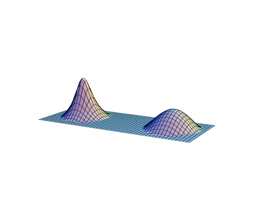
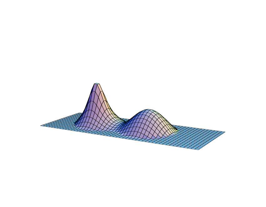
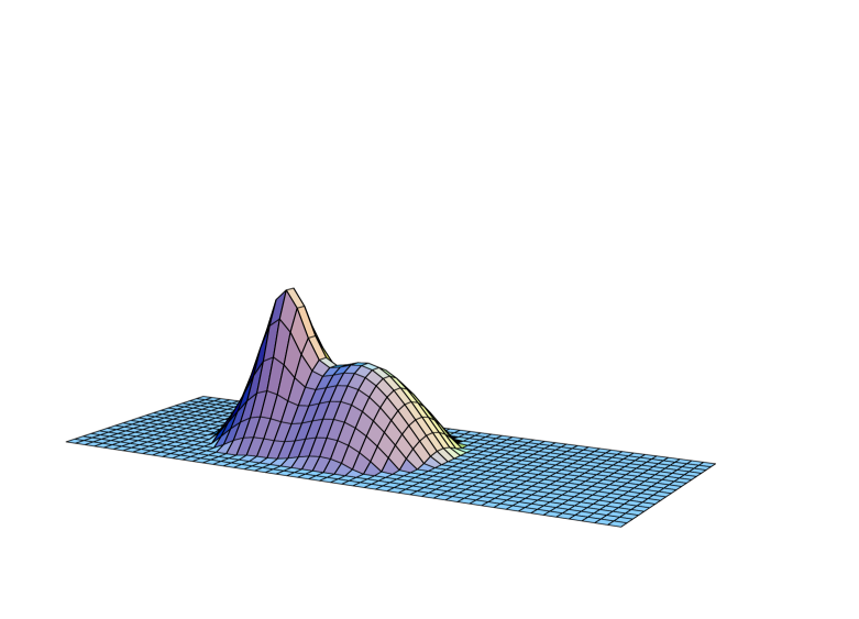
Figure 3: Shown are caloron profiles for $\omega=0.125$ (${\cal{T}}=1$), with $\rho=0.8,1.2,1.6$ (from bottom to top). This illustrates the growing separation of the two lumps with $\rho$. Once the constituents are separated, the lumps are spherically symmetric and do not change their shape upon further separation. Vertically is plotted the action density at $x_{0}=0$, on equal logarithmic scales for all profiles. They were cut off at an action density below $1/e^{2}$.

One can show in this limit that they have unit, but opposite, magnetic charges and that the two lumps have spatial scales proportional to respectively $1/\bar{\omega}$ and $1/\omega$ (see sect. 7). Their action densities (or energy densities in this static limit) scale with $\bar{\omega}^{4}$ and $\omega^{4}$. After integration, this results in monopole masses of respectively $16\pi^{2}\bar{\omega}/{\cal{T}}$ and $16\pi^{2}\omega/{\cal{T}}$ for the two lumps, their mass ratio is therefore $\bar{\omega}/\omega$. The total energy, simply obtained by addition, indeed conforms with the unit topological charge of the solution. For $\omega=0$ or $\omega={\scriptstyle{{1\over 2}}}$, the second lump is absent and the solution is spherically symmetric. For generic $\omega$, the solution has only an axial symmetry around the axis $\hat{a}$ connecting the two lumps. For $\omega={\scriptstyle{{1\over 4}}}$, the lumps are equally sized, and the solution has a mirror symmetry in the plane perpendicular to $\hat{a}$, see fig. 4.

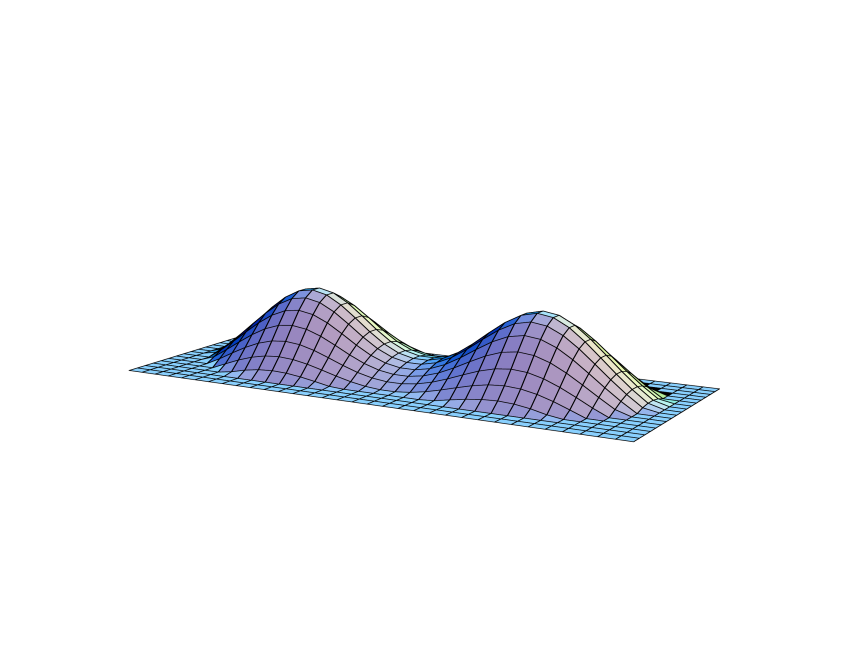
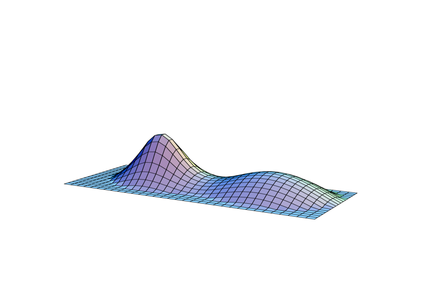
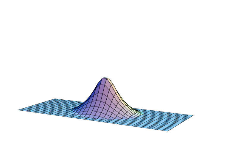
Figure 4: Profiles for calorons at $\omega\!=\!0$, 0.125, 0.25 (from left to right) with $\rho={\cal{T}}=1$. The axis connecting the lumps, separated by a distance $\pi$ (for $\omega\neq 0$), corresponds to the direction of $\hat{a}$. The other direction indicates the distance to this axis, making use of the axial symmetry of the solutions. The mass ratio of the two lumps is approximately $\omega/\bar{\omega}$, i.e. zero (no second lump), a third and one (equal masses), for the respective values of $\omega$. Vertically is plotted the action density at $x_{0}=0$, on equal logarithmic scales for all profiles. They were cut off at an action density below $1/e$.

These aspects can be readily retrieved by inspecting eq. (55), and in particular eq. (62), for the limit of large $\rho$ and realising that $r$ and $s$ are the centre off mass radii of the constituent monopoles. If $\rho$ is small, the caloron is best described in terms of the instanton picture, whereas for large $\rho$ the two-monopole picture is more appropriate. For the constituent picture of oppositely charged BPS monopoles to be correct, the field has to behave like a magnetic (and electric) dipole at large distances. Indeed one easily finds that the field strength decays as $1/|\vec{x}|^{3}$ for distances much larger than $\pi\rho^{2}/{\cal{T}}$. Note that for $\omega=0$ we have the standard Harrington-Shepard caloron [11], which in the limit of large $\rho$ was already shown by Rossi [32] to become the standard BPS monopole (after a singular gauge transformation).

Interpreting the Nahm data (eq. (41)) as the juxtaposition of two sub-intervals of lengths $2\omega$ and $2\bar{\omega}$ respectively, with constant Nahm connections $\hat{A}(z)$, leads to a more indirect way of understanding the composite nature of the caloron. Indeed, $\hat{A}=0$ gives the standard BPS-monopole, adding a constant merely translates the solution in space. Thus, each interval gives rise to a BPS monopole on ${\rm I\kern-1.79993ptR}^{3}\times S^{1}$, and we can in a good approximation add the two connections corresponding to the two sub-intervals. The $\rho^{2}$ dependence of $\hat{A}(z)$ explains the large separation of the constituent lumps for large $\rho$. As the lengths of the intervals are given by the asymptotic Higgs vacuum expectation value of the corresponding monopoles, the mass ratio $\bar{\omega}/\omega$ of the lumps is easily explained by noting that the mass of a BPS monopole is proportional to the Higgs vacuum expectation value. The above interpretation underlies the approach taken in ref. [10]. The expression for the gauge potential given there is precisely the sum alluded to above, plus gauge-like terms and gauge transformations required for glueing them together.

6 The moduli space

The moduli space ${\cal{M}}$ of the caloron solutions has as its coordinates $\xi$ and $\zeta$. We should include the global gauge degrees of freedom ($SU(2)$ for trivial and $U(1)$ for non-trivial holonomies), so as to make the solution space hyperKähler. The moduli space of these so-called framed calorons is a product of the base manifold ${\rm I\kern-1.79993ptR}^{3}\times S^{1}$, parametrised by $\xi$ and the (Taub-NUT) space parametrised by $\zeta$, forming the non-trivial part of the moduli space and describing the relative coordinates of the two constituent monopoles, quite similar to that for the two-monopole moduli space [33]. It should be noted that $\zeta\rightarrow-\zeta$, corresponding to the center of the $SU(2)$, leaves $A_{\mu}(x)$ invariant, such that we have to mod-out this symmetry to obtain the space of framed calorons.

The metric on this space is given by the Riemannian metric on the gauge theory configuration space, restricted to the space of solutions. The metric is then given by ($g_{M}^{\mu\nu}=\delta^{\mu\nu}$ being the flat metric on $M={{\rm I\kern-1.79993ptR}^{3}\times S^{1}}$)

$$g_{\cal{M}}(Z,Z^{\prime})=\int_{M}g_{M}^{\mu\nu}{\rm tr}\left(Z^{\dagger}_{\mu}(x)Z^{\prime}_{\nu}(x)\right).$$ (72)

with $Z_{\mu}$ and $Z^{\prime}_{\mu}$ two vectors tangent to the space of caloron solutions. The gauge structure requires them to be transverse to gauge deformations, thereby satisfying the background (or Coulomb) gauge condition

$$D^{\mu}\!(A)Z_{\mu}=0.$$ (73)

The requirement that $A_{\mu}+Z_{\mu}$ is self-dual leads to the so-called deformation equations

$$D_{[\mu}Z_{\nu]}={\scriptstyle{{1\over 2}}}\epsilon_{\mu\nu\alpha\beta}D_{[\alpha}Z_{\beta]},$$ (74)

and in the algebraic gauge we have to require in addition (see eq. (2))

$$Z_{\mu}(x+1)=e^{2\pi i\vec{\omega}\cdot\vec{\tau}}Z_{\mu}(x)e^{-2\pi i\vec{\omega}\cdot\vec{\tau}}.$$ (75)

The tangent vectors (zero modes) can be found by varying the caloron solution with respect to the coordinates $\xi$ and $\zeta$, which will automatically satisfy the deformation equation eq. (74) and periodicity eq. (75), but generally one has to apply an infinitesimal gauge transformation $\Phi$, compatible with eq. (75), to transform to the Coulomb gauge, eq. (73). Hence,

$$Z^{r}_{\mu}=\delta_{r}A_{\mu}+D_{\mu}\Phi^{r},$$ (76)

where the label $r$ indicates the parameters (or coordinates) of the moduli space. For the metric (eq. (72)) to exist, zero modes should of course be normalisable.

For instantons on ${\rm I\kern-1.79993ptR}^{4}$, the zero modes can be determined within the ADHM formalism [29]. Thus one can calculate the metric in terms of the ADHM data. This reflects the fact that the Nahm transformation (and the ADHM construction) is a hyperKähler isometry [19, 17]. We have

$$\delta\Delta=\left(\begin{array}[]{c}\delta\lambda\\ \delta B\end{array}\right)\equiv\left(\begin{array}[]{c}c\\ Y\end{array}\right)=C,$$ (77)

and for the calorons, in addition periodicity (eq. (75)) requires

$$Y_{m,n}=Y_{m-1,n-1},\quad c_{m+1}=e^{2\pi i\vec{\omega}\cdot\vec{\tau}}c_{m}.$$ (78)

In terms of the deformation $C$ of the ADHM data, the zero mode reads [29]

$$Z_{\mu}=v^{\dagger}(x)C{\bar{\sigma}}_{\mu}f_{x}u(x)\phi^{-{\scriptstyle{{1\over 2}}}}(x)-\phi^{-{\scriptstyle{{1\over 2}}}}(x)u^{\dagger}(x)f_{x}\sigma_{\mu}C^{\dagger}v(x).$$ (79)

and

$$D^{\mu}Z_{\mu}(x)=\phi^{-1}u^{\dagger}(x)f_{x}\sigma_{\mu}\left(C^{\dagger}\Delta(x)-\Delta^{\dagger}(x)C\right)\bar{\sigma}_{\mu}f_{x}u(x).$$ (80)

(Note that for $W=W_{\mu}\sigma_{\mu}$, $\sigma_{\mu}W\bar{\sigma}_{\mu}=4W_{0}=2{\rm tr}W$.) Combining the deformation of the quadratic ADHM constraint (as the ${\Im m}$ part) with the Coulomb gauge condition (as the ${\Re e}$ part), imposes

$$(\Delta^{\dagger}(x)C)=(\Delta^{\dagger}(x)C)^{t}.$$ (81)

To satisfy the Coulomb gauge condition, the ${\Re e}$ part of this equation being equivalent to

$${\rm tr}(\Delta^{\dagger}(x)C-C^{\dagger}\Delta(x))=0,$$ (82)

one has only the $T$ invariance of eq. (17) available (i.e. the $U(1)$ gauge invariance of $\hat{A}$), since a global gauge rotation would distort the framing. We write $T\in O(k)$ as $T=\exp(-\delta X)$, with $\delta X^{t}=-\delta X$. Like $T$, also $\delta X$ has to satisfy $\delta X_{m,n}=\delta X_{m-n}$, and can be interpreted as the Fourier coefficients of a gauge function $\delta\hat{g}(z)$ on the circle. We now write the zero modes $C$ in ADHM language as a variation of $\Delta$ plus a compensating gauge transformation,

$$C=\delta\Delta+\delta_{X}\Delta,\quad\delta_{X}\Delta=\left(\begin{array}[]{c}\lambda\delta X\\ \left[B,\delta X\right]\end{array}\right).$$ (83)

Inserting this in eq. (82) we find

$${\rm tr}\left((\delta\Delta^{\dagger})\Delta-\Delta^{\dagger}\delta\Delta-2\delta X\Lambda+\left[B^{\dagger},\delta X\right]B-B^{\dagger}\left[B,\delta X\right]\right)=0,$$ (84)

where we used that $\left[\Lambda,\delta X\right]=0$, since the gauge symmetry (described by $\delta X$) is abelian. After Fourier transformation, with $\delta(z-z^{\prime})\delta\hat{X}(z)=\sum_{m,n}X_{m,n}(x)e^{2\pi i(mz-nz^{\prime})}$, this equation reads

$$-\frac{1}{4\pi^{2}}\frac{d^{2}\delta\hat{X}(z)}{dz^{2}}+|\zeta|^{2}(\delta(z-\omega)+\delta(z+\omega))\delta\hat{X}(z)=\frac{i}{2}\rho^{2}(\delta(z-\omega)-\delta(z+\omega))\hat{\omega}\cdot\vec{\Sigma},$$ (85)

using that with the help of the Maurer-Cartan one-forms, eq. (67), we can write

$${\rm tr}\left((\delta\zeta\bar{\zeta}-\zeta\delta\bar{\zeta})\hat{\omega}\!\cdot\!\vec{\sigma}\right)=4\hat{\omega}^{a}\eta^{a}_{\mu\nu}\zeta_{\mu}\delta\zeta_{\nu}=2\rho^{2}\hat{\omega}\cdot\vec{\Sigma}.$$ (86)

The solution to the differential equation for $\delta\hat{X}(z)$ gives the infinitesimal gauge transformations needed to go to Coulomb gauge. One finds

$$\delta\hat{X}(z)=-2\pi^{2}i\rho^{2}\hat{\omega}\cdot\vec{\Sigma}(1+8\pi^{2}\omega\bar{\omega}\rho^{2})^{-1}\int_{0}^{z}\Theta_{\omega}(z^{\prime})dz^{\prime}$$ (87)

which is a zig-zag wave (see fig. 5), vanishing at $2z\in{\rm Z\!\!Z}$ and taking its extremal values at $z=\pm\omega$,

$$\delta\hat{X}_{\omega}\equiv\pm\delta\hat{X}(\pm\omega)=-4i\pi^{2}\omega\bar{\omega}\rho^{2}\hat{\omega}\cdot\vec{\Sigma}(1+8\pi^{2}\omega\bar{\omega}\rho^{2})^{-1},$$ (88)

Note that for the variations with respect to the caloron position, $\xi$, no compensating gauge transformation is needed.

Figure 5: The function $\int^{z}_{0}\Theta_{\omega}(z^{\prime})dz^{\prime}$.

In order to evaluate the metric, eq. (72), it is sufficient to compute $g_{\cal{M}}(Z,Z)$ for $Z$ related to an arbitrary deformation of the moduli parameters, as determined by $C$ in eq. (83) and eq. (87). For this we employ the following relation due to Osborn [29]

$${\rm tr}(Z^{\dagger}_{\mu}(x)Z^{\phantom{\dagger}}_{\mu}(x))=-{\scriptstyle{{1\over 2}}}\partial^{2}\,{\rm tr}\,{\rm Tr}\,\left(C^{\dagger}(2-\Delta(x)f_{x}\Delta^{\dagger}(x))Cf_{x}\right)$$ (89)

$$\hskip 81.09052pt=-{\scriptstyle{{1\over 2}}}\partial^{2}\,{\rm tr}\,{\rm Tr}\,\left(2(c^{\dagger}c+Y^{\dagger}Y)f_{x}-(c^{\dagger}\lambda+Y^{\dagger}B(x))f_{x}(\lambda^{\dagger}c+B^{\dagger}(x)Y)f_{x}\right),$$

which is derived from eq. (79), making use of eq. (81). We introduce the Fourier transforms $\hat{c}(z)\equiv\sum_{m}\exp(2\pi imz)c_{m}$ and $\hat{Y}(z)$, with $\delta(z-z^{\prime})\hat{Y}(z)=\sum_{m,n}e^{2\pi i(mz-nz^{\prime})}Y_{m,n}$, such that

$$\hat{c}(z) = \delta\hat{\lambda}(z)+\hat{\lambda}(z)\delta\hat{X}(z)=P_{+}\delta(z-\omega)(\delta\zeta+\zeta\delta\hat{X}_{\omega})+P_{-}\delta(z+\omega)(\delta\zeta-\zeta\delta\hat{X}_{\omega}),$$

$$\quad\hat{Y}(z) = \frac{1}{2\pi i}\left(\delta\hat{A}(z)+{\frac{d}{dz}}\delta\hat{X}(z)\right)$$ (90)

$$= \delta\xi+\pi\left(\delta\bar{\zeta}\hat{\omega}\cdot\vec{\sigma}\zeta+\bar{\zeta}\hat{\omega}\cdot\vec{\sigma}\delta\zeta-\rho^{2}\hat{\omega}\cdot\vec{\Sigma}(1+8\pi^{2}\omega\bar{\omega}|\zeta|^{2})^{-1}\right)\Theta_{\omega}(z).$$

We may use the special structure of $\hat{c}(z)$ and $\hat{\lambda}(z)$ (eq. (38)) - formed out of the combinations $\delta(z\mp\omega)P_{\pm}$, with $P_{\pm}^{2}=P_{\pm}$ and $P_{\pm}P_{\mp}=0$ - to deduce

$$\hat{c}^{\dagger}(z)\hat{c}(z^{\prime})\!=\!\delta(z-z^{\prime})\hat{c}^{\dagger}(z)\!<\!\hat{c}\!>,\quad\hat{c}^{\dagger}(z)\hat{\lambda}(z^{\prime})\!=\!\delta(z-z^{\prime})\hat{c}^{\dagger}(z)\!<\!\hat{\lambda}\!>,\quad<\!h\!>\equiv\!\!\int_{S^{1}}\!h(z)dz.$$ (91)

For calorons, this allows us to turn Osborn’s equation into

$${\rm tr}(Z^{\dagger}_{\mu}(x)Z^{\phantom{\dagger}}_{\mu}(x))=-\partial^{2}\int_{S_{1}}dz~{}{\rm tr}\left(\left[\hat{Y}^{\dagger}(z)\hat{Y}(z)+\hat{c}^{\dagger}(z)<\!\hat{c}\!>\right]\hat{f}_{x}(z,z)\right)$$ (92)

$$\hskip 85.35826pt+{\scriptstyle{{1\over 2}}}\partial^{2}\int_{S^{1}}dzdz^{\prime}~{}{\rm tr}\left([\hat{\cal{C}}(z)+\hat{\cal{Y}}_{x}(z)]\hat{f}_{x}(z,z^{\prime})[\hat{\cal{Y}}_{x}^{\dagger}(z^{\prime})+\hat{\cal{C}}^{\dagger}(z^{\prime})]\hat{f}_{x}(z^{\prime},z)\right),$$

with

$$\hat{\cal{Y}}_{x}(z)=(2\pi i)^{-1}\hat{Y}^{\dagger}(z)\hat{D}_{x}(z),\quad\hat{\cal{C}}(z)=\hat{c}^{\dagger}(z)<\!\hat{\lambda}\!>.$$ (93)

When integrating over space-time, the $\partial_{0}^{2}$ part does not contribute due to periodicity. The integral is therefore reduced to a boundary term at spatial infinity, $|\vec{x}|\rightarrow\infty$. In this limit $\rho^{2}$ can be neglected and the two radii $r$ and $s$ in eq. (45) become equal. In particular in this limit the potential in eq. (44) equals $|\vec{x}|^{2}$, independent of $z$. From this one concludes that asymptotically $\hat{f}_{x}(z,z^{\prime})$ becomes a function of $z-z^{\prime}$ and therefore that $\hat{D}_{x}(z)\hat{f}_{x}(z,z^{\prime})\hat{D}^{\dagger}_{x}(z^{\prime})=4\pi^{2}\delta(z-z^{\prime})+{\cal{O}}(r^{-1})$. This can also be deduced from the asymptotic form of $\hat{f}_{x}(z,z^{\prime})$ in eq. (56), which implies $\hat{f}_{x}(z,z)=\pi/r+{\cal{O}}(r^{-2})$. Thus $\int_{S^{1}}dz^{\prime}~{}{\rm tr}[\hat{\cal{Y}}_{x}(z)\hat{f}_{x}(z,z^{\prime})\hat{\cal{Y}}_{x}(z^{\prime})\hat{f}_{x}(z,z^{\prime})]$ $={\rm tr}[\hat{Y}^{\dagger}(z)\hat{Y}(z)\hat{f}_{x}(z,z)]$, to be combined with the first term in eq. (92). Using eq. (91), we also have $\int_{S^{1}}dz^{\prime}~{}{\rm tr}[\hat{\cal{C}}(z)\hat{f}_{x}(z,z^{\prime})\hat{\cal{C}}^{\dagger}(z^{\prime})\hat{f}_{x}(z,z^{\prime})]\!=$ ${\rm tr}[<\!\hat{c}^{\dagger}\!><\!\hat{\lambda}\!><\!\hat{\lambda}^{\dagger}\!>\hat{c}(z)\hat{f}^{2}_{x}(z,z)]={\cal{O}}(r^{-2})$, and $2\pi i\int_{S^{1}}dz^{\prime}~{}{\rm tr}[\hat{\cal{Y}}(z)\hat{f}_{x}(z,z^{\prime})\hat{\cal{C}}^{\dagger}(z^{\prime})\hat{f}_{x}(z,z^{\prime})]\!=$ $\sum_{s=\pm}{\rm tr}[\hat{Y}^{\dagger}(z)D_{x}(z)f_{x}(z,s\omega)<\!\hat{\lambda}^{\dagger}\!><\!\hat{c}\!>P_{s}f_{x}(s\omega,z)]$, which after integration over $z$ is ${\cal{O}}(r^{-2})$. Only those terms that are ${\cal{O}}(r^{-1})$ will contribute and we obtain the following remarkably simple result

$$g_{\cal{M}}(Z,Z)=2\pi^{2}{\rm tr}(<\hat{Y}^{\dagger}\hat{Y}>+2<\hat{c}^{\dagger}><\hat{c}>).$$ (94)

Inserting eq. (6) gives the metric (we put $\hat{\omega}=\hat{e}_{3}$)

$$ds^{2}=2\pi^{2}\left\{2d\xi_{\mu}d\xi^{\mu}\!+\!(1\!+\!8\pi^{2}\omega\bar{\omega}\rho^{2})\left(4d\rho^{2}\!+\!\rho^{2}\left(\Sigma^{2}_{1}\!+\!\Sigma^{2}_{2}\right)\right)\!+\!\rho^{2}(1\!+\!8\pi^{2}\omega\bar{\omega}\rho^{2})^{-1}\Sigma^{2}_{3}\right\}.$$ (95)

The first part describes the flat metric of the base manifold ${\rm I\kern-1.79993ptR}^{3}\times S^{1}$, the remainder forms the non-trivial part of the metric. They separate because $\int\Theta_{\omega}(z)dz=0$, see eq. (42).

We introduce a “radial” coordinate $X$ and “mass” parameter $M$

$$X^{2}=8\pi^{2}\rho^{2},\quad M^{-2}={16\omega\bar{\omega}},$$ (96)

and rewrite the non-trivial part of the moduli space metric as

$$ds^{2}=\left(1+\frac{X^{2}}{16M^{2}}\right)\left(dX^{2}+{\scriptstyle{{1\over 4}}}X^{2}(\Sigma^{2}_{1}+\Sigma^{2}_{2})\right)+{\scriptstyle{{1\over 4}}}X^{2}\left(1+\frac{X^{2}}{16M^{2}}\right)^{-1}\Sigma^{2}_{3}.$$ (97)

This metric is the Taub-NUT metric [34] as given in [35]. It is a self-dual Einstein manifold [36, 37] and is hyperKähler [33, 38]. The latter property is inherited from the hyperKähler structure of the base manifold ${\rm I\kern-1.79993ptR}^{3}\times S^{1}$, preserved by the self-duality equations [19]. Therefore, the ${SU(2)}$ moduli space for calorons becomes

$${\cal{M}}_{\rm framed}=({\rm I\kern-1.79993ptR}^{3}\times S^{1})\times{\rm Taub}\!-\!{\rm NUT}/Z_{2}.$$ (98)

Note that $Z_{2}$ corresponds with $\zeta=q=\pm 1$, i.e. the center of the SU(2) gauge group. With $\zeta\rightarrow-\zeta$ leaving the gauge fields unchanged, this gives rise to an orbifold singularity (at $\zeta\!=\!0$) and $({\rm I\kern-1.79993ptR}^{3}\!\times\!S^{1})\!\times\!{\rm Taub}\!-\!{\rm NUT}$ is a double cover of ${\cal{M}}_{\rm framed}$.

For small $\rho$ or $\omega$, when $X^{2}/M^{2}\rightarrow 0$, the metric becomes that of ${\rm I\kern-1.79993ptR}^{4}$, since ${\scriptstyle{{1\over 4}}}(\Sigma^{2}_{1}+\!\Sigma_{2}^{2}+\!\Sigma_{3}^{2})$ (see eq. (67)) is the metric on the unit three-sphere. With $\rho\rightarrow 0$ corresponding to ${\cal{T}}\rightarrow\infty$, this describes the moduli space of a charge one instanton on ${\rm I\kern-1.79993ptR}^{4}$, whereas for $\omega=0$ we have the standard Harrington-Shepard caloron moduli space. In both cases this is parametrised by the scale and ${SU(2)}$ group orientation (to make the moduli space hyperKähler) and ${\cal{M}}_{\rm framed}={\rm I\kern-1.79993ptR}^{4}\!\times\!{\rm I\kern-1.79993ptR}^{4}/Z_{2}$, see ref. [19, 39].

For large $\rho$ (i.e. large $X$), or equivalently for ${\cal{T}}\rightarrow 0$, Taub-NUT space is a squashed $S^{3}$, that is $S^{2}\times S^{1}$, with $S^{1}$ a non-trivial (Hopf) fibration over $S^{2}$. This is best studied by introducing a radial coordinate $R$ through $X^{2}=8MR$, which brings the Taub-NUT metric to the form [36]

$$ds^{2}=\left(1+\frac{2M}{R}\right)(dR^{2}+R^{2}(d\theta^{2}+\sin^{2}\theta d\phi^{2}))+4M^{2}\left(1+\frac{2M}{R}\right)^{-1}(d\Upsilon+\cos\theta d\phi)^{2},$$ (99)

also familiar from the (spatial part of the) Kaluza-Klein monopole solution [40]. Since $\Upsilon\in[0,4\pi]$ we read-off from the asymptotic form of the metric that the compactification radius equals $4M$. At large $\rho$, ${\cal{M}}_{\rm framed}$ is therefore of the form $({\rm I\kern-1.79993ptR}^{3}\!\times\!S^{1})\!\times\!({\rm I\kern-1.79993ptR}^{3}\!\times^{\prime}\!S^{1})/Z_{2}$. It is natural to view this as the product space of two single BPS monopole moduli spaces. The first ${\rm I\kern-1.79993ptR}^{3}$ represents the centre of mass and the second the relative coordinates. The first $S^{1}$ corresponds to $x_{0}$ and can be seen as a global $U(1)$. The other gives the relative $U(1)$ orientation on which the $Z_{2}$ acts. This $Z_{2}$ does not act on the positions, as the monopoles have in general different masses and are hence not identical objects. A similar description is valid for the ${SU(2)}$ two-monopole moduli space, see ref. [41, 33]. At large separations its metric is precisely of the Taub-NUT form, but with a negative mass parameter $M$, as was shown by Manton [42], using the asymptotic form of the interactions. The complete metric was constructed by Atiyah and Hitchin (see ref. [33]) in terms of elliptic integrals, using its symmetries and hyperKähler structure.

Finally it is interesting to note that the moduli space of an $SU(3)$ monopole with maximal symmetry breaking to $U(1)\!\times\!U(1)$ and charges $(1,1)$ (see ref. [43, 44]) is Taub-NUT with a positive mass parameter, as for the caloron. This is not surprising, as its Nahm data are precisely those of the caloron. For an $SU(3)$ monopole with maximal symmetry breaking there are two sub-intervals $[\mu_{1},\mu_{2}]$ and $[\mu_{2},\mu_{3}]$. On each sub-interval, $\hat{A}$ has dimension one and is therefore constant, due to the Nahm equations. The matching at $\mu_{2}$, implied by the delta function singularity, is of the correct form (defining ${\scriptstyle{{1\over 2}}}\rho^{2}$), and implies we can identify $\mu_{1}$ with $\mu_{3}$ (defining ${\cal{T}}$) with correct matching as well. As the metric can be formulated in terms of the Nahm data, we would indeed expect the metric to be the same.

7 Discussion

The interpretation of the ADHM data for a periodic instanton as the Fourier coefficients of the Nahm transformed Weyl operator extends naturally to higher charges and other gauge groups [45]. For charge one calorons in $SU(N)$ the determination of the Green’s function remains a problem of quantum mechanics on the circle with a piecewise constant potential (on $N$ sub-intervals, separated by delta functions). Also our formalism to compute the metric on the moduli space can be generalised. Due to the relation with the ADHM approach, one may wonder [6] if there is some advantage in obtaining monopole solutions from the calorons by sending certain scales to infinity - in the limit of which the solution becomes static and constituents separate. For higher charges the Nahm bundle is no longer abelian and the construction is more complicated. For generalisations to further compactifications, e.g. ${\rm I\kern-1.79993ptR}^{2}\times T^{2}$ and ${\rm I\kern-1.79993ptR}\times T^{3}$ (see ref. [18]), note that the ’t Hooft ansatz [28] diverges when summing over more than one direction. This will correspond to all holonomies trivial and one may well have no solutions in that case. A dramatic particular example of a non-existence proof for charge one instantons is $T^{4}$, see ref. [17], a situation where indeed an existence proof of Taubes [46] does not hold.

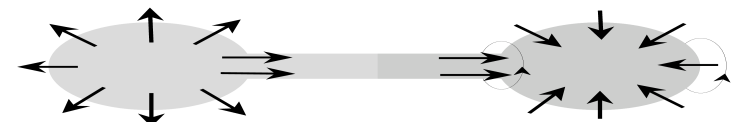
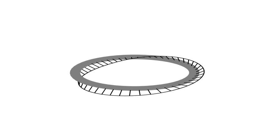
Figure 6: The non-contractible loop is constructed from two oppositely charged monopoles by rotating one of them, as indicated on the left. On the right is a closed monopole line, rotating its frame when completing the circle.

We now recall briefly Taubes’s arguments for building gauge fields with topological charge one out of monopole fields [9, 47]. Although his construction was within the standard model with a genuine Higgs field, the same argument applies to the caloron case, using $A_{0}$ as the Higgs field. As we saw in sect. 2 (eqs. (10,11)), non-trivial ${SU(2)}$ monopole fields can be classified by the winding number $k_{1}=-k_{2}$ of maps from $S^{2}$ to $SU(2)/U(1)\sim S^{2}$. We consider at this point configurations at a fixed time $t$, $\Psi=\{A_{\mu}(\vec{x})\}$. In the sector where the net winding vanishes, we study a one-parameter family of configurations, $\Psi_{t}=\{A_{\mu}(\vec{x},t)\}$ (the parameter can, but need not, be seen as the time $t$). When this configuration is made out of monopoles with opposite charges, in a suitable gauge the isospin orientations behave as shown in fig. 6, sufficiently far from the core of both monopoles. We note that the arrows match in the “throat” of the configuration. This remains true if we rotate only one of the monopoles around the axis of the throat. Clearly, the net magnetic winding remains zero, but the fields of two monopoles will no longer cancel when brought together, despite the fact that the long range abelian components do cancel. The non-contractible loop is now constructed by letting $t$ affect a full rotation.

Taubes describes this by creating a monopole anti-monopole pair, bringing them far apart, rotating one of them over a full rotation and finally bringing them together to annihilate. The four dimensional configuration constructed this way is topologically non-trivial. Since an anti-monopole travelling forward in time is a monopole travelling backwards in time, we can describe the same as a closed monopole line (or loop). It represents a topologically non-trivial configuration when the monopole makes a full rotation while moving along the closed monopole line (see fig. 6). The non-trivial topology discussed by Taubes [9] ($\pi_{1}(M_{0}(S^{2};S^{2}))={\rm Z\!\!Z}$) is just the Hopf fibration, except that now it is more natural to see $S^{1}$ as the base manifold and $S^{2}$ as the fibre, which rotates (twists) while moving along the circle formed by the closed monopole line . The only topological invariant available to characterise this homotopy type is precisely the Pontryagin index.

We mentioned that the short range components of the fields can not be fully cancelled due to the non-trivial “twist” along the monopole line, so they have to be responsible for the Pontryagin index. Indeed, in the computation of the total topological charge of our configurations as the integral over $\partial_{\mu}^{2}\partial_{\nu}^{2}\log\psi$ (eq. (63)), the massive component of the field gives rise to

$$\psi=2e^{4\pi(r\bar{\omega}+s\omega)}(1+{\cal{O}}(|\vec{x}|^{-1}))=2e^{2\pi|\vec{x}|}(1+{\cal{O}}(|\vec{x}|^{-1})),\quad\partial_{\mu}^{2}\log\psi=4\pi/|\vec{x}|+{\cal{O}}(|\vec{x}|^{-4}),$$ (100)

and thus yields the surviving boundary term, but at the same time does not contribute to the action density, since $\partial_{\mu}^{2}|\vec{x}|^{-1}=0$.

We now inspect more closely the monopole content of our calorons. For this we choose $\rho/{\cal{T}}$ large, such that the monopoles are well separated and static. We have two world lines of monopoles running in opposite directions (due to their opposite charges), closed due to the periodic boundary conditions. At smaller separations the solutions are far from static, with the attractive force driving the constituents together, after which they annihilate. In that case the world lines form a single closed monopole line, as mentioned above. It should be noted though, that for small $\rho/{\cal{T}}$ the constituents become rather extended. Nevertheless, such closed monopole lines are characterised by rotation of the local monopole field over precisely one full rotation when completing the circle, since our solution has unit topological charge. It prevents the field from decaying to the trivial configuration. It is this “twist” that provides the closed monopole line its stability.

Before continuing, we observe that the calorons are given in a singular gauge, as is usual for the ADHM construction. The function $\hat{\psi}$ (eq. (52)) has an isolated zero at $x=0$. This can be traced to the zero-mode in $B-x$, responsible for the non-trivial topology of the solution. This singularity is easily seen to be removed by a gauge transformation, locally of the form $x/|x|$ (viewing $x$ as a quaternion). We now assume that $\omega\bar{\omega}\neq 0$ and consider the region outside the core of both monopoles, i.e. $r\bar{\omega}>1$ and $s\omega>1$. In this region

$$\phi = \frac{r+s+\pi\rho^{2}}{r+s-\pi\rho^{2}}+{\cal{O}}(e^{-8\pi\,{\rm min}(s\omega,r\bar{\omega})}),$$ (101)

$$\tilde{\chi} = \frac{4\pi\rho^{2}}{(r+s+\pi\rho^{2})^{2}}\left\{re^{-4\pi r\bar{\omega}}e^{-2\pi ix_{0}}+se^{-4\pi s\omega}\right\}\left(1+{\cal{O}}(e^{-8\pi\,{\rm min}(s\omega,r\bar{\omega})})\right).$$

Substituting this in eq. (57) we find the solution to be time independent and abelian, up to exponential correction

$$A_{0}=\frac{i}{2}\tau_{3}\partial_{3}\log\phi,\quad A_{k}=\frac{i}{2}\tau_{3}\epsilon_{kj3}\partial_{j}\log\phi,$$ (102)

$$E_{k}=F_{k0}=\frac{i}{2}\tau_{3}\partial_{k}\partial_{3}\log\phi,\quad B_{k}=\epsilon_{kij}\partial_{i}A_{j}=\frac{i}{2}\tau_{3}\left(\partial_{k}\partial_{3}\log\phi-\delta_{k3}\partial_{j}^{2}\log\phi\right).$$

For convenience we rotate $\hat{a}$ to $\hat{e}_{3}$. Self-duality, $\vec{E}\!=\!\vec{B}$, requires $\log\phi$ to be harmonic. We first note that when neglecting the exponential corrections, $\phi^{-1}$ vanishes on the interval $-2\pi\rho^{2}\omega\leq x_{3}\leq 2\pi\rho^{2}\bar{\omega}$ at $x_{1}\!=\!x_{2}\!=\!0$ (we denote the characteristic function on this interval by $\chi_{\omega}(x_{3})$). A careful analysis reveals $\partial_{j}^{2}\log\phi\!=\!-4\pi\delta(x_{1})\delta(x_{2})\chi_{\omega}(x_{3})$ (that it vanishes away from the zeros of $\phi^{-1}$ follows by a direct computation). The term $-\frac{i}{2}\tau_{3}\delta_{k3}\partial_{j}^{2}\log\phi$ in the expression for the magnetic field corresponds precisely to the Dirac string singularity, carrying the return flux. One finds that $\partial_{k}E_{k}\!=\!\partial_{k}B_{k}\!=\!\frac{i}{2}\tau_{3}\partial_{3}\partial_{j}^{2}\log\phi\!=\!2\pi i\tau_{3}(\delta_{3}(\vec{s})\!-\!\delta_{3}(\vec{r}))$, when ignoring this return flux, which in the full theory is absent [48] (indeed as noted before $\phi^{-1}$ has only an isolated zero at $x=0$, corresponding to a gauge singularity).

Finally, to confirm our expectations it remains to identify the rotation of one of the monopoles so as to guarantee the topologically non-trivial nature of the configuration. Inspecting the behaviour in the core region of the monopoles, described by $\tilde{\chi}$ in eq. (101), gives the following factorisation

$$\tilde{\chi}=\chi^{(1)}(r)+e^{-2\pi ix_{0}}\chi^{(2)}(s).$$ (103)

While one of the monopoles has a static core, the other has a time dependent phase rotation - equivalent to a (gauge) rotation - precisely of the type required to form a non-contractible loop, as the phase makes a full rotation when closing by the periodic boundary conditions in the time direction.

Although interpreting $A_{0}$ as the Higgs field allows one to introduce monopoles in pure gauge theory, there are some subtle differences. In the static limit the BPS equations imply $F_{i0}=D_{i}A_{0}$ and we would be tempted to call the solution a dyon. In the Higgs model dyons are constructed by taking $A_{0}$ proportional to the Higgs field $\Phi$ [2, 49]. By a time dependent gauge transformation $A_{0}$ can be gauged to zero. This gauge transformation is generated by $A_{0}$, precisely the unbroken generator, as $A_{0}$ is proportional to the Higgs field. The resulting electric field is now given by $\partial_{0}A_{i}$ and is not quantised. In the abelian Higgs model $B_{i}=D_{i}\Phi$ and $E_{i}=-\partial_{0}A_{i}$. In pure gauge theory it makes, however, no sense to separate $D_{i}\Phi=D_{i}A_{0}$ from $\partial_{0}A_{i}$. Gauge invariance requires that they occur in the combination $F_{i0}=D_{i}A_{0}-\partial_{0}A_{i}$. The electric field is necessarily fixed and quantised as soon as we interpret $A_{0}$ as the Higgs field. Nevertheless, we can consider dyons also in pure gauge theories, but for this we have to add a term proportional to $\theta F\tilde{F}$ to the lagrangian [50]. The electric charge is now proportional to $\theta$, so no longer quantised. But, unlike in the Higgs model, it is the same for all monopoles.

We note that in the Higgs model the construction of the non-contractible loop generates an electric charge due to the (gauge) rotation along the closed monopole line, when interpreting the loop parameter as time. The electric charge is proportional to the rate of rotation and can vary along the monopole line. However, integrated along a closed monopole line the charge is fixed and proportional to the number of rotations, which hence plays the role of a winding number. In pure gauge theory this winding can not be read off from the long range field components, but for both cases the fields in the core are responsible for the Pontryagin number (an abelian field can not contribute to this topological charge).

There is a natural context in which the analogy with the Higgs model is more precise. For this we have to add time as a fifth dimension, such that four dimensional space is compactified on a circle. In the limit of zero compactification radius (${\cal{T}}\rightarrow 0$) our solutions become genuine monopoles and can obtain dyonic charges in the sense of Julia and Zee [49]. It is in this context that Taub-NUT metric describes the scattering of oppositely charged monopoles on ${\rm I\kern-1.79993ptR}^{3}\times S^{1}$, in exactly the same way as the Atiyah-Hitchin metric describes the scattering of like-charged monopoles on ${\rm I\kern-1.79993ptR}^{3}$ [51, 33].

Monopoles appear also in the context of ’t Hooft’s abelian projection [16] as (gauge) singularities. The lesson we have learned from the above analysis is that in order to include the non-trivial topological charge, important for fermion zero modes, breaking of the axial $U(1)$ symmetry [22] and presumably for chiral symmetry breaking, one needs to keep some information on the behaviour near the core of these monopoles. This allows one to combine the attractiveness of the dual superconductor picture of confinement [52] in terms of monopole degrees of freedom, with the success of the instanton liquid model [53]. There have been many attempts to make an effective monopole model for the long range confining properties of QCD, see e.g. ref. [54]. Also there have been many studies in lattice gauge theory, using the idea of abelian projection implemented by the so-called maximal abelian gauge [55], in order to extract the monopole content of the theory. It was observed that the string tension is saturated by the monopole fields [56]. More recently it was found that after abelian projection instantons contain closed monopole lines [57]. As emphasised in ref. [58], in the light of Taubes’s construction this was to be expected. Here we have shown in more detail how one can make fields with non-zero topological charge out of monopole degrees of freedom, with as example the well defined setting of calorons with non-trivial Polyakov loop. What is minimally required is a frame associated to each monopole, whose rotation is a topological invariant for closed monopole lines. Such closed monopole lines can shrink, but one will be left over with what represents an instanton. It would be interesting to build a hybrid model based on the instanton liquid and monopoles, and see how successful it is in capturing the appropriate phenomenology.

To conclude, it is sensible to take the monopole content of instantons serious in the broader context sketched here. Our gauge invariant method of investigating the monopoles inside an instanton is somewhat destructive (but reversible). First we heat the instanton just a little. Then we add a non-trivial value of the Polyakov loop at infinity, without disturbing the instanton significantly (true for ${\cal{T}}$ sufficiently large). Now we have to squeeze (or heat) it hard. Out come the two constituent monopoles, in a direction determined by the choice we have made for the Polyakov loop at infinity (which does not change under heating). The new caloron solutions can be studied on the lattice by taking all links in the time direction, at the spatial boundary of the lattice, equal to $U_{0}=\exp(2\pi i\vec{\omega}\cdot\vec{\tau}/N_{0})$ (in lattice units ${\cal{T}}$ equals $N_{0}$). One can look for solutions using improved cooling [59] (to prevent calorons to disappear due to scaling violations). When interested in seeing the monopole constituents one may just as well take the time direction to be one lattice spacing ($N_{0}=1$). The lattice study of ref. [60] hints at regular monopole solutions in pure gauge theory, although with a vanishing electric component, not what we would expect for our constituents.

Appendix

In this appendix we present the result for the Green’s function $G_{x}=(B^{\dagger}(x)B(x))^{-1}$, which after Fourier transformation satisfies the equation

$$\left\{\!\!\left(\!\frac{1}{2\pi i}{\frac{d}{dz}}\!-\!x_{0}\right)^{\!\!2}\!\!+\!s^{2}\chi_{[-\omega,\omega]}(z)\!+\!r^{2}\chi_{[\omega,1-\omega]}(z)\!-\!\frac{\rho^{2}}{2}\hat{\omega}\!\cdot\!\vec{\tau}(\delta(z\!\!-\!\!\omega)\!-\!\delta(z\!\!+\!\!\omega))\!\right\}\!\!\hat{G}_{x}(z,z^{\prime})=\delta(z-z^{\prime}),$$ (104)

with $r$ and $s$ given as in eq. (45). Its solution is given by

$$\hskip-14.22636pt\hat{G}_{x}(z,z^{\prime})=\chi_{[-\omega,\omega]}(z^{\prime})\left(\chi_{[-\omega,\omega]}(z)\hat{G}^{d}_{x}(z,z^{\prime},r,s,\omega)+\chi_{[\omega,1-\omega]}(z)\hat{G}^{o}_{x}(z,z^{\prime},r,s,\omega)\right)$$ (105)

$$\hskip-2.84526pt+\chi_{[\omega,1\!-\!\omega]}(z^{\prime}))\left(\chi_{[\omega,1-\omega]}(z)\hat{G}^{d}_{x}({\scriptstyle{{1\over 2}}}\!-\!z,{\scriptstyle{{1\over 2}}}\!-\!z^{\prime},s,r,\bar{\omega})^{*}\!+\!\chi_{[-\omega,\omega]}(z)\hat{G}^{o}_{x}(\!z^{\prime},z,r,s,\omega)^{*}\right).$$

Like for $\hat{f}_{x}$ the diagonal component $\hat{G}^{d}_{x}(z,z^{\prime})$ is only defined strictly for $z,z^{\prime}\in[-\omega,\omega]$ and the off-diagonal component $\hat{G}^{o}_{x}(z,z^{\prime})$ only for $z\in[\omega,1\!-\!\omega]$ and $z^{\prime}\in[-\omega,\omega]$. For $z$ or $z^{\prime}$ outside of these intervals, one first has to map back to the interval $[-\omega,1\!-\!\omega]$, using periodicity.

$$\hskip-14.22636pt\hat{G}^{d}_{x}(z,z^{\prime},r,s,\omega)=e^{2\pi ix_{0}(z-z)}\pi(rs\hat{\psi})^{-1}\Big{\{}e^{-2\pi ix_{0}{\rm sign}(z-z^{\prime})}r\sinh(2\pi s|z\!-\!z^{\prime}|)$$ (106)

$$\qquad+s^{-1}\sinh(4\pi r\bar{\omega})\Big{[}\pi s\rho^{2}\hat{\omega}\cdot\vec{\tau}\sinh(2\pi s(z+z^{\prime}))\!+\!{\scriptstyle{{1\over 2}}}(s^{2}\!-\!r^{2}\!+\!\pi^{2}\rho^{4})\cosh(2\pi s(z\!+\!z^{\prime}))$$

$$\qquad+\!{\scriptstyle{{1\over 2}}}(s^{2}\!+\!r^{2}\!-\!\pi^{2}\rho^{4})\cosh(2\pi s(2\omega\!-\!|z\!-\!z^{\prime}|))\Big{]}\!+\!r\cosh(4\pi r\bar{\omega})\sinh(2\pi s(2\omega\!-\!|z\!-\!z^{\prime}|))\Big{\}},$$

$$\hskip-14.22636pt\hat{G}^{o}_{x}(z,z^{\prime},r,s,\omega)=e^{2\pi ix_{0}(z-z^{\prime})}\pi(rs\hat{\psi})^{-1}\Big{\{}\pi\rho^{2}\hat{\omega}\cdot\vec{\tau}\sinh(2\pi r(1\!-\!z-\!\omega))\sinh(2\pi s(z^{\prime}\!+\!\omega))$$

$$\qquad+\!r\cosh(2\pi r(z\!-\!1\!+\!\omega))\sinh(2\pi s(z^{\prime}\!+\!\omega))-s\sinh(2\pi r(z\!-\!1+\!\omega))\cosh(2\pi s(z^{\prime}\!+\!\omega))$$

$$\qquad e^{-2\pi ix_{0}}\Big{[}s\sinh(2\pi r(z\!-\!\omega))\cosh(2\pi s(z^{\prime}\!-\!\omega))-r\cosh(2\pi r(z\!-\!\omega))\sinh(2\pi s(z^{\prime}\!-\!\omega))$$

$$\hskip 170.71652pt+\pi\rho^{2}\hat{\omega}\cdot\vec{\tau}\sinh(2\pi r(z\!-\!\omega))\sinh(2\pi s(z^{\prime}\!-\!\omega))\Big{]}\Big{\}}.$$

In particular,

$$\hat{G}_{x}(\omega,-\omega)=\pi(rs\hat{\psi})^{-1}e^{4\pi ix_{0}\omega}\left\{e^{-2\pi ix_{0}}r\sinh(4\pi s\omega)+s\sinh(4\pi r\bar{\omega})\right\},$$ (107)

$$\hat{G}_{x}(\pm\omega,\pm\omega)\!=\!\pi(rs\hat{\psi})^{-1}\Big{\{}s\sinh(4\pi r\bar{\omega})\cosh(4\pi s\omega)\!+\!r\sinh(4\pi s\omega)\cosh(4\pi r\bar{\omega})$$

$$\hskip 221.93158pt\pm\pi\rho^{2}\hat{\omega}\!\cdot\!\vec{\tau}\sinh(4\pi r\bar{\omega})\sinh(4\pi s\omega)\Big{\}}.$$

which can be used to verify eq. (51) as derived from eq. (19), and eq. (64).

References

• [1] M.F. Atiyah, N.J. Hitchin, V.G. Drinfeld, Yu. I. Manin, Phys. Lett. 65 A (1978) 185.
• [2] E.B. Bogomol’ny, Yad. Fiz. 24 (1976) 861; Sov. J. Nucl. 24 (1976) 449; M.K. Prasad and C.M. Sommerfield, Phys. Rev. Lett. 35 (1975) 760.
• [3] N.S. Manton, Nucl. Phys. B126 (1977) 525.
• [4] C. Montonen and D. Olive, Phys. Lett. 72B (1977) 117.
• [5] H. Garland and M.K. Murray, Commun. Math. Phys. 120 (1988) 335.
• [6] K. Lee and P. Yi, Phys. Rev. D56 (1997) 3711 (hep-th/9702107).
• [7] W. Nahm, Self-dual monopoles and calorons, in: Lect. Notes in Physics. 201, eds. G. Denardo, e.a. (1984) p. 189.
• [8] T.C. Kraan and P. van Baal, Exact T-duality between calorons and Taub-NUT spaces, Phys. Lett. B428 (1998) 268 (hep-th/9802049).
• [9] C. Taubes, Morse theory and monopoles: topology in long range forces, in: Progress in gauge field theory, eds. G. ’t Hooft et al, (Plenum Press, New York, 1984) p. 563.
• [10] K. Lee, Instantons and magnetic monopoles on $R^{3}\times S^{1}$ with arbitrary simple gauge groups, hep-th/9802012; K. Lee and C. Lu, SU(2) calorons and magnetic monopoles, hep-th/9802108.
• [11] B.J. Harrington and H.K. Shepard, Phys. Rev. D17 (1978) 2122; ibid. D18 (1978) 2990.
• [12] D.J. Gross, R.D. Pisarski and L.G. Yaffe, Rev. Mod. Phys. 53 (1983) 43.
• [13] P. van Baal, Twisted boundary conditions: a non-perturbative probe for pure non-abelian gauge theories, (Ph.D. thesis, Utrecht, July 1984).
• [14] W. Nahm, Phys. Lett. 90B (1980) 413.
• [15] W. Nahm, All self-dual multimonopoles for arbitrary gauge groups, CERN preprint TH-3172 (1981), published in Freiburg ASI 301 (1981); The construction of all self-dual multimonopoles by the ADHM method, in: β€œMonopoles in quantum field theory”, eds. N. Craigie, e.a. (World Scientific, Singapore, 1982), p.87.
• [16] G. ’t Hooft, Nucl. Phys. B190[FS3] (1981) 455; Physica Scripta 25 (1982) 133.
• [17] P.J. Braam and P. van Baal, Commun. Math. Phys. 122 (1989) 267.
• [18] P. van Baal, Nucl. Phys. B(Proc. Suppl.) 49 (1996) 238 (hep-th/9512223).
• [19] S.K. Donaldson and P.B. Kronheimer, The Geometry of Four-Manifolds, (Clarendon Press, Oxford, 1990).
• [20] M.F. Atiyah, I.M. Singer, Ann. Math. 93 (1971) 119.
• [21] C. Callias, Commun. Math. Phys. 62 (1978) 213; R. Bott and R. Seeley, Commun. Math. Phys. 62 (1978) 235.
• [22] G. ’t Hooft, Phys. Rev. D14 (1976) 3432.
• [23] E. Corrigan and P. Goddard, Ann. Phys. (N.Y.) 154 (1984) 253.
• [24] N.J. Hitchin, Commun. Math. Phys. 89 (1983) 145; J. Hurtubise and M.K. Murray, Commun. Math. Phys. 122 (1989) 35.
• [25] H. Nakajima, Monopoles and Nahm’s Equations, in β€œEinstein metrics and Yang-Mills connections”, Sanda, 1990, eds. T. Mabuchi and S. Mukai, (Dekker, 1993, New York).
• [26] M.F. Atiyah, Geometry of Yang-Mills fields, Fermi lectures, (Scuola Normale Superiore, Pisa, 1979).
• [27] E.F. Corrigan, D.B. Fairlie, S. Templeton and P. Goddard, Nucl. Phys. B140 (1978) 31.
• [28] G. ’t Hooft, unpublished, quoted in R. Jackiw, C. Nohl, C. Rebbi, Phys. Rev. D15 (1977) 1642; R. Rajaraman, Solitons and Instantons, (North-Holland, Amsterdam, 1982).
• [29] H. Osborn, Ann. Phys. (N.Y.) 135 (1981) 373.
• [30] T.C. Kraan, Nahm’s transformation and instantons on $R^{3}\times S^{1}$, poster presented at the 2nd DRSTP symposium, Dalfsen, The Netherlands, 5-6 June, 1997 (unpublished).
• [31] E.T. Whitakker and G.N. Watson, A course in modern analysis, (Cambridge Univ. Press, 1927) p. 169.
• [32] P. Rossi, Nucl. Phys. B149 (1979) 170.
• [33] M.F. Atiyah and N.J. Hitchin, The Geometry and Dynamics of Magnetic Monopoles, (Princeton Univ. Press, 1988).
• [34] E.T. Newman, T. Unti and L. Tamburino, J. Math. Phys. 4 (1963) 915.
• [35] S. Hawking, in: General Relativity, an Einstein centenary survey, eds. S. Hawking and W. Israel, (Cambridge Univ. Press, 1979) p. 774.
• [36] S. Hawking, Phys. Lett 60A (1977) 81.
• [37] T. Eguchi and A.T. Hanson, Phys. Lett. 74B (1978) 249; G. Gibbons and C. Pope, Commun. Math. Phys. 66 (1979) 267.
• [38] N.J. Hitchin, A. Karlhede, U. LindstrΓΆm and M. Roček, Commun. Math. Phys. 108 (1987) 535.
• [39] J.P. Gauntlett and J.A. Harvey, S-Duality and the Spectrum of Magnetic Monopoles in Heterotic String Theory, hep-th/9407111.
• [40] R. Sorkin, Phys. Rev. Lett. 51 (1983) 87; D. Gross and M.Perry, Nucl. Phys. B226 (1983) 29.
• [41] G.W. Gibbons and N.S. Manton, Nucl. Phys. B274 (1986) 183.
• [42] N.S. Manton, Phys. Lett. 154B (1985) 397 [Err. 157B (1985) 475].
• [43] S.A. Connell, The dynamics of the SU(3) charge (1,1) magnetic monopole (1991), ftp://maths.adelaide.edu.au/pure/murray/oneone.tex, unpublished preprint.
• [44] J.P. Gauntlett and D.A. Lowe, Nucl. Phys. B472 (1996) 194 (hep-th/9601085); K. Lee, E.J. Weinberg and P. Yi, Phys. Lett. B376 (1996) 97 (hep-th/9601097).
• [45] K. Lee and P. Yi, Dyons in $N=4$ supersymmetric theories and three-pronged strings, hep-th/9804174.
• [46] C. Taubes, J. Diff. Geom. 19 (1984) 517.
• [47] C. Taubes, Commun. Math. Phys. 86 (1982) 257, 299.
• [48] G. ’t Hooft, Nucl. Phys. B79 (1974) 276; A.M. Polyakov, JETP Lett. 20 (1974) 194.
• [49] B. Julia and A. Zee, Phys. Rev. D11 (1975) 2227.
• [50] E. Witten, Phys. Lett. 86B (1979) 283.
• [51] N. Manton, Phys. Lett. 110B (1982) 54.
• [52] G. ’t Hooft, in: β€œHigh Energy Physics”, EPS conference, Palermo, 1975, ed. A. Zichichi (Editrice Compositori, Bologna, 1976); S. Mandelstam, Phys. Rept. 23C (1976) 245
• [53] E. Shuryak, Phys. Rep. 264 (1996) 357; T. SchΓ€fer and E. Shuryak, Rev. Mod. Phys. 70 (1998) 323 (hep-ph/9610451).
• [54] J. Smit and A. van der Sijs, Nucl. Phys. B355 (1991) 603.
• [55] A.S. Kronfeld, G. Schierholz and U.J. Wiese, Nucl. Phys. B293 (1987) 461.
• [56] T. Suzuki and I. Yotsuyanagi, Phys.Rev. D42 (1990) 4257; M. Polikarpov, Nucl.Phys. B(Proc. Suppl.)53 (1997) 134 (hep-lat/9609020), and ref. therein.
• [57] M.N. Chernodub and F.V. Gubarev, JETP Lett. 62 (1995) 100 (hep-th/9506026); A. Hart and M. Teper, Phys.Lett. B372(1996) 261 (hep-lat/9511016); V. Bornyakov and G. Schierholz, Phys. Lett. B384(1996)190 hep-lat/9605019); R.C. Brower, K.N. Orginos and Ch.-I. Tan, Phys. Rev. D55 (1997) 6313 (hep-th/9610101)
• [58] P. van Baal, Nucl. Phys. B(Proc. Suppl.) 63A-C (1998) 126 (hep-lat/9709066).
• [59] M. GarcΓ­a PΓ©rez, A. GonzΓ‘lez-Arroyo, J. Snippe and P. van Baal, Nucl.Phys. B413(1994)535-553 (hep-lat/9309009).
• [60] M.L. Laursen and G. Schierholz, Z. Phys. C38 (1988) 501.