Quantum and string shape fluctuations
in the dual Monopole Nambu–Jona–Lasinio model with dual Dirac strings

Abstract

The magnetic monopole condensate is calculated in the dual Monopole Nambu–Jona–Lasinio model with dual Dirac strings suggested in Refs.[1,2] as a functional of the dual Dirac string shape. The calculation is carried out in the tree approximation in the scalar monopole–antimonopole collective excitation field. The integration over quantum fluctuations of the dual–vector monopole–antimonopole collective excitation field around the Abrikosov flux line and string shape fluctuations are performed explicitly. We claim that there are important contributions of quantum and string shape fluctuations to the magnetic monopole condensate.

Institut für Kernphysik, Technische Universität Wien,
Wiedner Hauptstr. 8-10, A-1040 Vienna, Austria

1 Introduction

In Refs.[1,2] there has been suggested the dual Monopole Nambu–Jona–Lasinio (MNJL) model with dual Dirac strings as a continuum analogy of Compact Quantum Electrodynamics (CQED) which is defined for lattices as nonlinear $U\,(1)$ gauge theory. It has a confining phase like QCD [3] and realizes confinement of “color” electric charges. Thereby, the investigation of CQED should help us to understand quark confinement. As has been shown in Ref.[4] the nonperturbative vacuum of CQED behaves like an effective dual superconductor with magnetic monopoles. Due to magnetic monopoles the electric flux between quarks rearranges and looks like the field produced by a dual Dirac string. As a result quarks interact via a linearly rising potential [5,6] that realizes quark confinement [7,8] and spontaneous breaking of chiral symmetry (SB$\chi$S) [8].

The NJL model [9] can be regarded as some kind of relativistic extension of the BCS (Bardeen–Cooper–Schrieffer) theory of superconductivity [10]. It also possesses a nonperturbative vacuum with a ground state of the same kind as in a superconductor in the superconducting phase. The latter has been the promoting idea of Refs.[1,2] to put the NJL–model to the foundation of a continuum space–time model realizing non–perturbative phenomena of CQED.

The MNJL–model is based on the Lagrangian, invariant under “color” magnetic $U(1)$ symmetry, of massless magnetic monopoles, self–coupled through local four–monopole interaction [1,2]:

$${\cal L}(x)=\bar{\chi}(x)i\gamma^{\mu}\partial_{\mu}\chi(x)+G[\bar{\chi}(x)\chi(x)]^{2}-G_{1}[\bar{\chi}(x)\gamma_{\mu}\chi(x)][\bar{\chi}(x)\gamma^{\mu}\chi(x)],$$ (1.1)

where $\chi(x)$ is a massless magnetic “color” monopole field, $G$ and $G_{1}$ are positive phenomenological constants responsible for the magnetic monopole condensation and the dual–“color” vector field mass, respectively.

The magnetic monopole condensation accompanies the creation of massive magnetic monopoles $\chi_{M}(x)$ with mass $M$, $\bar{\chi}\chi$–collective excitations with quantum numbers of scalar Higgs meson field $\sigma$ with mass $M_{\sigma}=2\,M$ and a massive dual–vector field $C_{\mu}$ with mass $M_{C}$ defined as [1,2]:

$$M^{2}_{C}=\frac{g^{2}}{2G_{1}}-\frac{g^{2}}{8\pi^{2}}[J_{1}(M)+M^{2}J_{2}(M)],$$ (1.2)

where $J_{1}(M)$ and $J_{2}(M)$ are quadratically and logarithmically divergent integrals [1,2]

$$J_{1}(M) = \int\frac{d^{4}k}{\pi^{2}i}\frac{1}{M^{2}-k^{2}}=\Lambda^{2}-M^{2}{\ell n}\Bigg{(}1+\frac{\Lambda^{2}}{M^{2}}\Bigg{)},$$

$$J_{2}(M) = \int\frac{d^{4}k}{\pi^{2}i}\frac{1}{(M^{2}-k^{2})^{2}}={\ell n}\Bigg{(}1+\frac{\Lambda^{2}}{M^{2}}\Bigg{)}-\frac{\Lambda^{2}}{M^{2}+\Lambda^{2}}.$$ (1.3)

Here $\Lambda$ is the ultra–violet cut–off. The mass of the massive magnetic monopole field $\chi_{M}(x)$ obeys the gap–equation [1,2]:

$$M=-2G<\bar{\chi}(0)\chi(0)>=\frac{GM}{2\pi^{2}}J_{1}(M).$$ (1.4)

After the integration over magnetic monopole degrees of freedom the effective Lagrangian containing quarks, antiquarks and the fields of scalar $\sigma$ and dual–vector $C_{\mu}$ collective excitations reads

$${\cal L}_{\rm eff}(x) = \frac{1}{4}F_{\mu\nu}(x)F^{\mu\nu}(x)+\frac{1}{2}M^{2}_{C}C_{\mu}(x)C^{\mu}(x)$$ (1.5)

$$+ \frac{1}{2}\partial_{\mu}\sigma(x)\partial^{\mu}\sigma(x)-\frac{1}{2}M^{2}_{\sigma}\sigma^{2}(x)\Bigg{[}1+\kappa\frac{\sigma(x)}{M_{\sigma}}\Bigg{]}^{2}$$

$$+ {\cal L}_{\rm free~{}quark}(x),$$

The coupling constants $g$ and $\kappa$ are related by the constraint

$$\frac{g^{2}}{12\pi^{2}}J_{2}(M)=\frac{\kappa^{2}}{8\pi^{2}}\,J_{2}(M)=1$$ (1.6)

or $\kappa^{2}=2g^{2}/3$ [1,2].

${\cal L}_{\rm free~{}quark}(x)$ is the kinetic term for the quark and antiquark,

$${\cal L}_{\rm free~{}quark}(x)=-\sum_{i=q,\bar{q}}m_{i}\int d{\tau}\Bigg{(}\frac{dX^{\mu}_{i}(\tau)}{d\tau}\frac{dX^{\nu}_{i}(\tau)}{d\tau}g_{\mu\nu}\Bigg{)}^{1/2}\delta^{(4)}(x-X_{i}(\tau)).$$ (1.7)

We consider quark and antiquark as classical point–like particles with masses $m_{q}=m_{\bar{q}}=m$, electric charges $Q_{q}=-Q_{\bar{q}}=Q$, and trajectories $X^{\nu}_{q}(\tau)$ and $X^{\nu}_{\bar{q}}(\tau)$, respectively. The field strength $F^{\mu\nu}(x)$ is defined [1,2] as $F^{\mu\nu}(x)={\cal E}^{\mu\nu}(x)-{{}^{*}}dC^{\mu\nu}(x)$, where $dC^{\mu\nu}(x)=\partial^{\mu}C^{\nu}(x)-\partial^{\nu}C^{\mu}(x)$, and ${{}^{*}}dC^{\mu\nu}(x)$ is the dual version, i.e., ${{}^{*}}dC^{\mu\nu}(x)=\frac{1}{2}\varepsilon^{\mu\nu\alpha\beta}dC_{\alpha\beta}(x)\,(\varepsilon^{0123}=1)$.

The “color” electric field strength ${\cal E}^{\mu\nu}(x)$, induced by a dual Dirac string, is defined following [1,2] as

$${\cal E}^{\mu\nu}(x)=Q\int\!\!\!\int d\tau d\sigma\Bigg{(}\frac{\partial X^{\mu}}{\partial\tau}\frac{\partial X^{\nu}}{\partial\sigma}-\frac{\partial X^{\nu}}{\partial\tau}\frac{\partial X^{\mu}}{\partial\sigma}\Bigg{)}\delta^{(4)}(x-X),$$ (1.8)

where $X^{\mu}=X^{\mu}(\tau,\sigma)$ represents the position of a point on the world sheet swept by the string. The sheet is parametrized by the internal coordinates ${-\infty}<\tau<{\infty}$ and $0\leq\sigma\leq\pi$, so that $X^{\mu}(\tau,0)=X^{\mu}_{-Q}(\tau)$ and $X^{\mu}(\tau,\pi)=X^{\mu}_{Q}(\tau)$ represent the world lines of an antiquark and a quark [1,2,5]. Within the definition Eq.(1.8) the tensor field ${\cal E}^{\mu\nu}(x)$ satisfies identically the equation of motion, $\partial_{\mu}F^{\mu\nu}(x)=J^{\nu}(x)$. The electric quark current $J^{\nu}(x)$ is defined as

$$J^{\nu}(x)=\sum_{i=q,\bar{q}}Q_{i}\int d\tau\frac{dX^{\nu}_{i}(\tau)}{d\tau}\delta^{(4)}(x-X_{i}(\tau)).$$ (1.9)

Hence, the inclusion of a dual Dirac string in terms of ${\cal E}^{\mu\nu}(x)$ defined by Eq.(1.8) satisfies completely the electric Gauss law of Dirac^′s extension of Maxwell ${}^{\prime}\,$s electrodynamics.

As has been shown in Refs.[1,2] the vacuum expectation values of time–ordered products of densities expressed in terms of the massless–monopole field, i.e., the magnetic monopole Green function

$$G\,(x_{1},\ldots,x_{n})=<{0}|{\rm T}(\bar{\chi}(x_{1})\Gamma_{1}\chi(x_{1})\ldots\bar{\chi}(x_{n})\,\Gamma_{n}\chi\,(x_{n}))|{0}>_{\rm conn.}\,,$$ (1.10)

where $\Gamma_{i}(i=1,\ldots,n)$ are the Dirac matrices, are given by [1,2]

$$G(x_{1},\ldots,x_{n})=<{0}|{\rm T}(\bar{\chi}(x_{1})\Gamma_{1}\chi(x_{1})\ldots\bar{\chi}(x_{n})\Gamma_{n}\chi(x_{n}))|{0}>_{\rm conn.}=$$

$$=^{(M)}\!<{0}|{\rm T}\Big{(}\bar{\chi}_{M}(x_{1})\Gamma_{1}\chi_{M}(x_{1})\ldots\bar{\chi}_{M}(x_{n})\Gamma_{n}\chi_{M}(x_{n})$$

$$\times\;e^{\displaystyle i\int d^{4}x\{-g\bar{\chi}_{M}(x)\gamma^{\nu}\chi_{M}(x)C_{\nu}(x)-\kappa\bar{\chi}_{M}(x)\chi_{M}(x)\sigma(x)+{\cal L}_{\rm int}[\sigma(x)]\}}\Big{)}|{0}>^{(M)}_{\rm conn.}.$$ (1.11)

Here $|{0}\!>^{(M)}$ is the wave-function of the nonperturbative vacuum of the MNJL–model in the condensed phase and $|{0}\!>$ the wave-function of the noncondensed perturbative vacuum. ${\cal L}_{\rm int}[\sigma(x)]$ describes self–interactions of the $\sigma$–field:

$${\cal L}_{\rm int}[\sigma(x)]=-\kappa\,M_{\sigma}\,\sigma^{3}(x)-\frac{1}{2}\,\sigma^{4}(x).$$ (1.12)

The self–interactions ${\cal L}_{\rm int}[\sigma(x)]$ provide $\sigma$–field loop contributions and can be dropped out in the tree $\sigma$–field approximation accepted in Refs. [1,2]. In the tree $\sigma$–field approximation the r.h.s. of Eq.(1) acquires the form

$$G(x_{1},\ldots,x_{n})=<{0}|{\rm T}(\bar{\chi}(x_{1})\Gamma_{1}\chi(x_{1})\ldots\bar{\chi}(x_{n})\Gamma_{n}\chi(x_{n}))|{0}>_{\rm conn.}=$$

$$=^{(M)}\!<{0}|{\rm T}\Big{(}\bar{\chi}_{M}(x_{1})\Gamma_{1}\chi_{M}(x_{1})\ldots\bar{\chi}_{M}(x_{n})\Gamma_{n}\chi_{M}(x_{n})$$

$$\times\;e^{\displaystyle i\int d^{4}x\Big{\{}-g\bar{\chi}_{M}(x)\gamma^{\nu}\chi_{M}(x)C_{\nu}(x)-\kappa\bar{\chi}_{M}(x)\chi_{M}(x)\sigma(x)\}}\Big{)}|{0}>^{(M)}_{\rm conn.}.$$ (1.13)

The tree $\sigma$–field approximation can be justified keeping massive magnetic monopoles very heavy, i.e. $M\gg M_{C}$. This corresponds to the London limit $M_{\sigma}=2\,M\gg M_{C}$ in the dual Higgs model with dual Dirac strings [11].

In Ref.[2] Eq.(1) has been applied to the computation of the magnetic monopole condensate $<\!\bar{\chi}(x)\chi(x);{\cal E}\!>$ in dependence of the dual Dirac string shape represented by the electric string tensor ${\cal E}^{\mu\nu}(x)$ Eq.(1.8). The magnetic monopole condensate $<\!\bar{\chi}(x)\chi(x);{\cal E}\!>$ has been calculated in the tree $\sigma$–field approximation neglecting the fluctuations of the dual–vector field $C_{\mu}$ around the Abrikosov flux line which satisfies the equation

$$(\Box+M^{2}_{C})C^{\nu}[{\cal E}(x)]=-\partial_{\mu}{{}^{*}{\cal E}}^{\mu\nu}(x),$$ (1.14)

and takes the form

$$C^{\nu}[{\cal E}(x)]=-\int d^{4}x^{\prime}\Delta(x-x^{\prime},M_{C})\partial^{\prime}_{\mu}{{}^{*}{\cal E}}^{\mu\nu}(x^{\prime}\,),$$ (1.15)

where $\Delta(x-x^{\prime},M_{C})$ is the Green function

$$\Delta(x-x^{\prime},M_{C})=\int\frac{d^{4}k}{(2\pi)^{4}}\frac{e^{\displaystyle-ik\cdot(x-x^{\prime}\,)}}{M^{2}_{C}-k^{2}-i0}.$$ (1.16)

In this paper we will calculate the magnetic monopole condensate $<\!\bar{\chi}(x)\chi(x);{\cal E}\!>$ in the tree $\sigma$–field approximation but taking into account quantum fluctuations of the dual–vector field $C_{\mu}$ around the Abriksov flux line $C^{\nu}[{\cal E}(x)]$. An important role of such fluctuations for the formation of the interquark potential has been pointed out in Ref. [12] within a dual Higgs model with dual Dirac strings.

This paper is organized as follows: In Sect.2 we calculate the magnetic monopole condensate in the tree $\sigma$–field approximation and explicitly integrate out quantum fluctuations of the dual–vector field $C_{\mu}$ around the Abrikosov flux line. In Sect.3 we calculate the contibution of the string shape fluctuations to the magnetic monopole condensate. In the Conclusion we discuss the obtained results.

2 Quantum dual–vector field fluctuations

In the tree $\sigma$–field approximation we determine the magnetic monopole condensate $<\!\bar{\chi}(x)\chi(x);{\cal E}\!>$ following [1] as

$$<\bar{\chi}(x)\chi(x);{\cal E}>-<\bar{\chi}(0)\chi(0)>=^{(M)}\!<{0}|{\rm T}\Big{(}\bar{\chi}_{M}(x)\chi_{M}(x)$$

$$\times\;e^{\displaystyle i\int d^{4}z\Big{\{}-g\bar{\chi}_{M}(z)\gamma^{\nu}\chi_{M}(z)C_{\nu}(z)-\kappa\bar{\chi}_{M}(z)\chi_{M}(z)\sigma(z)\}}\Big{)}|{0}>^{(M)}_{\rm conn.},$$ (2.1)

where the r.h.s. of Eq.(2) should vanish at $C_{\mu}=\sigma=0$.

The time ordering operator and vacuum wave–function act on the massive magnetic monopole fields $\chi_{M}$ and the fields of collective excitations $\sigma$ and $C_{\mu}$.

The calculation of vacuum expectation values of time–ordered products of the dual–vector fields is convenient to perform by means of the path integral method

$$<\bar{\chi}(x)\chi(x);{\cal E}>-<\bar{\chi}(0)\chi(0)>=\frac{1}{Z}\int{\cal D}C_{\mu}e^{\displaystyle i\int d^{4}z\,{\cal L}_{\rm eff}[C_{\mu}(z)]}\,{}^{(M)}\!<{0}|{\rm T}\Big{(}\bar{\chi}_{M}(x)\chi_{M}(x)$$

$$\times\;e^{\displaystyle i\int d^{4}z\Big{\{}-g\bar{\chi}_{M}(z)\gamma^{\nu}\chi_{M}(z)C_{\nu}(z)-\kappa\bar{\chi}_{M}(z)\chi_{M}(z)\sigma(z)\}}\Big{)}|{0}>^{(M)}_{\rm conn.},$$ (2.2)

where $Z$ is a normalization factor determined as

$$Z=\int{\cal D}C_{\mu}e^{\displaystyle i\int d^{4}z\,{\cal L}_{\rm eff}[C_{\mu}(z)]}.$$ (2.3)

The effective Lagrangian ${\cal L}_{\rm eff}[C_{\mu}(z)]$ is defined by the part of the effective Lagrangian Eq.(1.5) related to the $C_{\mu}$–field:

$${\cal L}_{\rm eff}[C_{\mu}(z)]=\frac{1}{4}F_{\mu\nu}(z)F^{\mu\nu}(z)+\frac{1}{2}M^{2}_{C}C_{\mu}(z)C^{\mu}(z).$$ (2.4)

In order to integrate out quantum fluctuations of the dual–vector field $C_{\mu}$ around the shape of the Abrikosov flux line we split the $C_{\mu}$–field into a classical field $C_{\mu}[{\cal E}(z)]$ induced by the Dirac string and quantum fluctuations $c_{\mu}(z)$ around that classical background. [12]:

$$C_{\mu}(z)=C_{\mu}[{\cal E}(z)]+c_{\mu}(z),$$ (2.5)

where $C_{\mu}[{\cal E}(z)]$ satisfies Eq.(1.14), and $c_{\mu}(z)$ are the fluctuations of the dual–vector field having a vanishing vacuum expectation value $<c_{\mu}(z)>=0$. Substituting the decomposition Eq.(2.5) in the Lagrangian Eq.(2.4) we arrive at the Lagrangian of the quantum fields $c_{\mu}(x)$ fluctuating around the Abrikosov flux line.

$${\cal L}_{\rm eff}[C_{\mu}(z)]={\cal L}_{\rm string}(z)+\frac{1}{2}\,c_{\mu}(z)\Big{[}(\Box+M^{2}_{C})\,g^{\mu\nu}-\partial^{\mu}\partial^{\nu}\Big{]}\,c_{\nu}(z),$$ (2.6)

where we have used Eq.(1.14). The Lagrangian of the dual Dirac string ${\cal L}_{\rm string}(z)$ is defined [5,11–13]

$$\int d^{4}z{\cal L}_{\rm string}(z)=\frac{1}{4}\,M^{2}_{C}\int\int d^{4}zd^{4}y{\cal E}_{\mu\alpha}(z)\Delta^{\alpha}_{\nu}(z-y,M_{C}){\cal E}^{\mu\nu}(y),$$ (2.7)

where $\Delta^{\alpha}_{\nu}(z-y,M_{C})=(g^{\alpha}_{\nu}+2\partial^{\alpha}\partial_{\nu}/M^{2}_{C})\Delta(z-y;M_{C})$.

Since the Lagrangian Eq.(2.5) is Gaussian with respect to the $c_{\mu}$–field, we are able to integrate out the $c_{\mu}$–field exactly.

Integrating over the $c_{\mu}$–field we reduce $<\bar{\chi}(x)\chi(x);{\cal E}>$ to the form:

$$<\bar{\chi}(x)\chi(x);{\cal E}>-<\bar{\chi}(0)\chi(0)>=^{(M)}\!<{0}|{\rm T}\Big{(}\bar{\chi}_{M}(x)\chi_{M}(x)\,$$

$$\times\;e^{\displaystyle-i\,\frac{1}{2}\,g^{2}\int\!\!\!\int d^{4}zd^{4}y\,[\bar{\chi}_{M}(z)\gamma^{\mu}\chi_{M}(z)]\,D_{\mu\nu}(z-z^{\prime},M_{C})\,[\bar{\chi}_{M}(z^{\prime}\,)\gamma^{\nu}\chi_{M}(z^{\prime}\,)]}$$

$$\times\;e^{\displaystyle i\int d^{4}z\{-g\bar{\chi}_{M}(z)\gamma^{\nu}\chi_{M}(z)C_{\nu}[{\cal E}(z)]-\kappa\bar{\chi}_{M}(z)\chi_{M}(z)\sigma(z)\}}\Big{)}|{0}>^{(M)}_{\rm conn.},$$ (2.8)

where $D_{\mu\nu}(z-z^{\prime},M_{C})$ is the Green function of the free $c_{\mu}$–field: $D_{\mu\nu}(z-z^{\prime},M_{C})=(g_{\mu\nu}+\partial_{\mu}\partial_{\nu}/M^{2}_{C})\,\Delta(z-z^{\prime},M_{C})$. Since herein we consider dual Dirac strings as classical objects the contribution of the Lagrangian of the dual Dirac strings ${\cal L}_{\rm string}(z)$ cancels out.

The integration over $\sigma$–field degrees of freedom in the tree approximation we perform following [2]. This yields

$$<\bar{\chi}(x)\chi(x);{\cal E}>-<\bar{\chi}(0)\chi(0)>=-\frac{\kappa^{2}}{4M^{3}}\,<\bar{\chi}(0)\chi(0)>\,^{(M)}\!<{0}|{\rm T}\Big{(}\bar{\chi}_{M}(x)\chi_{M}(x)$$

$$\times\;e^{\displaystyle-i\frac{1}{2}g^{2}\int\!\!\!\int d^{4}zd^{4}z^{\prime}[\bar{\chi}_{M}(z)\gamma^{\mu}\chi_{M}(z)]\,D_{\mu\nu}(z-z^{\prime};M_{C})\,[\bar{\chi}_{M}(z^{\prime}\,)\gamma^{\nu}\chi_{M}(z^{\prime}\,)]}$$

$$\times\;e^{\displaystyle-i\,g\int d^{4}z\,[\bar{\chi}_{M}(z)\gamma^{\nu}\chi_{M}(z)]\,C_{\nu}[{\cal E}(z)]}\Big{)}|{0}>^{(M)}_{\rm conn.},$$ (2.9)

For the calculation of the vacuum expectation value in the r.h.s of Eq.(2) we assume that the massive magnetic monopole fields $\chi_{M}(x)$ are almost on–mass shell. It is valid due to a very large mass of the monopole fields. In this case the transfer momenta are small compared with the mass of the dual–vector field $M_{C}$. By virtue these assumptions we can reduce the four–monopole interaction in Eq.(2) to a point–like interaction.

$$<\bar{\chi}(x)\chi(x);{\cal E}>-<\bar{\chi}(0)\chi(0)>=-\frac{\kappa^{2}}{4M^{3}}\,<\bar{\chi}(0)\chi(0)>\,^{(M)}\!<0|{\rm T}\Big{(}\bar{\chi}_{M}(x)\chi_{M}(x)$$

$$\times\;e^{\displaystyle-i\int d^{4}z\Bigg{\{}\frac{g^{2}}{2M^{2}_{C}}[\bar{\chi}_{M}(z)\gamma^{\mu}\chi_{M}(z)]^{2}+g\,[\bar{\chi}_{M}(z)\gamma^{\nu}\chi_{M}(z)]\,C_{\nu}[{\cal E}(z)]\Bigg{\}}}\Big{)}|0>^{(M)}_{\rm conn.}.$$ (2.10)

Thus, since $M\gg M_{C}$ the vacuum averaging over the massive magnetic monopole fields can be represented by the momentum integrals [2] related to the magnetic monopole diagrams depicted in Fig. 1 and Fig. 2:

$${}^{(M)}\!<0|{\rm T}\Big{(}\bar{\chi}_{M}(x)\chi_{M}(x)$$

$$\times\;e^{\displaystyle-i\int d^{4}z\Bigg{\{}\frac{g^{2}}{2M^{2}_{C}}[\bar{\chi}_{M}(z)\gamma^{\mu}\chi_{M}(z)]^{2}+g\,[\bar{\chi}_{M}(z)\gamma^{\nu}\chi_{M}(z)]\,C_{\nu}[{\cal E}(z)]\Bigg{\}}}\Big{)}|0>^{(M)}_{\rm conn.}=$$

$$=-\frac{1}{16\pi^{2}}\int\frac{d^{4}k}{\pi^{2}i}{\rm tr}\Bigg{\{}\frac{1}{M-\hat{k}+g\hat{C}[{\cal E}(x)]}-\frac{1}{M-\hat{k}}\Bigg{\}}$$

$$-\frac{1}{16\pi^{2}}\int\frac{d^{4}k}{\pi^{2}i}{\rm tr}\Bigg{\{}\frac{1}{M-\hat{k}+g\hat{C}[{\cal E}(x)]}\frac{1}{M-\hat{k}+g\hat{C}[{\cal E}(x)]}\gamma_{\mu_{1}}\Bigg{\}}$$

$$\times\sum^{\infty}_{n=1}\Bigg{(}\frac{g^{2}}{2M^{2}_{C}}\Bigg{)}^{n}\Bigg{(}\frac{1}{16\pi^{2}}\Bigg{)}^{(n-1)}\int\frac{d^{4}k_{1}}{\pi^{2}i}{\rm tr}\Bigg{\{}\frac{1}{M-\hat{k}_{1}+g\hat{C}[{\cal E}(x)]}\gamma_{\mu_{1}}\frac{1}{M-\hat{k}_{1}+g\hat{C}[{\cal E}(x)]}\gamma_{\mu_{2}}\Bigg{\}}$$

$$\ldots\int\frac{d^{4}k_{n-1}}{\pi^{2}i}{\rm tr}\Bigg{\{}\frac{1}{M-\hat{k}_{n-1}+g\hat{C}[{\cal E}(x)]}\gamma_{\mu_{n-1}}\frac{1}{M-\hat{k}_{n-1}+g\hat{C}[{\cal E}(x)]}\gamma_{\mu_{n}}\Bigg{\}}$$

$$\times\;\frac{1}{16\pi^{2}}\int\frac{d^{4}k_{n}}{\pi^{2}i}{\rm tr}\Bigg{\{}\gamma_{\mu_{n}}\frac{1}{M-\hat{k}_{n}+g\hat{C}[{\cal E}(x)]}\Bigg{\}}+\dots.$$ (2.11)

The first term in the r.h.s. of Eq.(2) has been calculated in Ref.[2] at the neglect of quantum fluctuations of the dual–vector field $C_{\mu}$, whereas the second term is fully due to these fluctuations. We calculate the second term keeping leading divergent contributions as it is accepted in the MNJL–model [1,2]. The ellipses denote the contribution of the diagrams depicted in Fig. 2b. This contribution is less important with respect to the contribution of the diagrams in Fig. 2a and below we adduce the result of the calculationof these diagrams without comments. The vacuum expectation value Eq.(2) amounts to

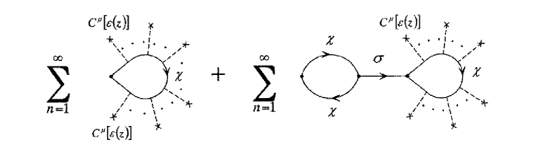
Figure 1: Magnetic monopole diagrams describing the magnetic monopole condensate around the dual Dirac string without fluctuations of the dual–vector field.

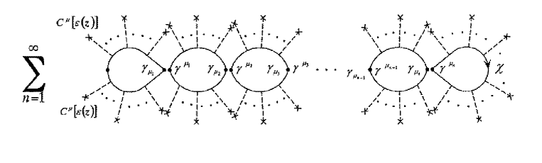
(a)

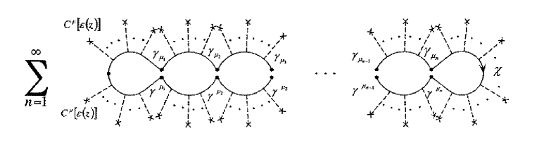
(b)

Figure 2: Magnetic monopole diagramms describing the contributions to the magnetic monopole condensate caused by the quantum fluctuations of the $C_{\mu}$–field.

$${}^{(M)}\!<0|{\rm T}\Big{(}\bar{\chi}_{M}(x)\chi_{M}(x)$$

$$\times\;e^{\displaystyle-i\int d^{4}z\Bigg{\{}\frac{g^{2}}{2M^{2}_{C}}[\bar{\chi}_{M}(z)\gamma^{\mu}\chi_{M}(z)]^{2}+g\,[\bar{\chi}_{M}(z)\gamma^{\nu}\chi_{M}(z)]\,C_{\nu}[{\cal E}(z)]\Bigg{\}}}\Big{)}|0>^{(M)}_{\rm conn.}=$$

$$=-\frac{M}{8\pi^{2}}\,g^{2}\,C_{\mu}[{\cal E}(x)]C^{\mu}[{\cal E}(x)]+\frac{M}{4\pi^{2}}\Bigg{\{}-\frac{g^{2}}{8\pi^{2}}[J_{1}(M)+M^{2}J_{2}(M)]\Bigg{\}}$$

$$\times\;\frac{g^{2}}{2M^{2}_{C}}\sum^{\infty}_{n=1}\Bigg{\{}\frac{1}{M^{2}_{C}}\frac{g^{2}}{16\pi^{2}}[J_{1}(M)+M^{2}J_{2}(M)]\Bigg{\}}^{(n-1)}C_{\mu}[{\cal E}(x)]C^{\mu}[{\cal E}(x)]\,=$$

$$=-\frac{M}{24\pi^{2}}\,\frac{\displaystyle M^{2}_{C}+\frac{g^{2}}{2G_{1}}}{\displaystyle M^{2}_{C}-\frac{g^{2}}{6G_{1}}}\,g^{2}\,C_{\mu}[{\cal E}(x)]C^{\mu}[{\cal E}(x)].$$ (2.12)

Here we have used the definitions of $M^{2}_{C}$ given by Eq.(1.2).

Thus, integrating out explicitly quantum fluctuations of the dual–vector field $C_{\mu}$ around the Abrikosov flux line and taking into account the contribution of the scalar field $\sigma$ in the tree approximation we obtain the magnetic monopole condensate in dependence on the shape of a dual Dirac string in the form:

$$<\bar{\chi}(x)\chi(x);{\cal E}>=<\bar{\chi}(0)\chi(0)>$$

$$\times\;\Bigg{\{}1-\frac{\kappa^{2}G_{1}}{1024\pi^{4}}\,\frac{<\bar{\chi}(0)\chi(0)>}{M^{3}}+\frac{\displaystyle M^{2}_{C}+\frac{g^{2}}{2G_{1}}}{\displaystyle M^{2}_{C}-\frac{g^{2}}{6G_{1}}}\,\frac{\kappa^{2}}{96\pi^{2}}\,\frac{1}{M^{2}}\,g^{2}\,C_{\mu}[{\cal E}(x)]C^{\mu}[{\cal E}(x)]\Bigg{\}}.$$ (2.13)

The second term in the braces of Eq.(2) is the result of the calculation of the diagrams in Fig. 2b. It may be seen that quantum fluctuations of a dual–vector field around the Abrikosov flux line give a substantial contribution to the magnetic monopole condensate. In order to retain the agreement with the results obtained within CQED [14] which testify the suppression of the magnetic monopole condensate in the region close to a dual Dirac string we have to impose the constraint $M^{2}_{C}>g^{2}/6G_{1}$.

3 Dual Dirac string shape fluctuations

The string shape fluctuations we define following [13,15] by $X^{\mu}\to X^{\mu}+\eta^{\mu}(X)$, where $\eta^{\mu}(X)$ describes fluctuations around the fixed surface $S$ swept by the shape $\Gamma$ and obeys the constraint $\eta^{\mu}(X)|_{\partial S}=0$ [13,15] at the boundary $\partial S$ of the surface $S$.

The magnetic monopole condensate defined by Eq.(2) and averaged over string shape fluctuations reads

$$<\bar{\chi}(x)\chi(x);{\cal E}>-<\bar{\chi}(0)\chi(0)>\Bigg{[}1-\frac{\kappa^{2}G_{1}}{1024\pi^{4}}\,\frac{<\bar{\chi}(0)\chi(0)>}{M^{3}}\Bigg{]}=$$

$$<\bar{\chi}(0)\chi(0)>\frac{\displaystyle M^{2}_{C}+\frac{g^{2}}{2G_{1}}}{\displaystyle M^{2}_{C}-\frac{g^{2}}{6G_{1}}}\,\frac{\kappa^{2}}{96\pi^{2}}\,\frac{1}{M^{2}}\,\frac{1}{Z_{\rm shape}}\int{\cal D}\eta_{\mu}\,e^{\displaystyle i\,\delta{\cal S}_{\rm N}[\eta]}\,g^{2}\,C_{\nu}\{\eta(x)\}C^{\nu}\{\eta(x)\},$$ (3.1)

where $Z_{\rm shape}$ is a normalization factor determined as

$$Z_{\rm shape}=\int{\cal D}\eta_{\mu}e^{\displaystyle i\,\delta{\cal S}_{\rm N}[\eta]}$$ (3.2)

and $\delta{\cal S}_{\rm N}[\eta]$ has been calculated in Ref.[13]:

$$\delta\,{\cal S}_{\rm N}[\eta]=\int\!\!\!\int d^{4}x\,d^{4}y\,\eta_{\alpha}(x)\,{\displaystyle O}^{\alpha\beta}(x-y)\,\eta_{\beta}(y)+\int d^{4}x\,\eta_{\alpha}(x)\,{\displaystyle O}^{\alpha}(x).$$ (3.3)

The operators ${\displaystyle O^{\alpha\beta}(x-y)}$ and ${\displaystyle O^{\alpha}(x)}$ are given by

$${\displaystyle O}^{\alpha\beta}(x-y) = ~{}~{}\frac{1}{2}\,\delta^{(4)}(x-y)\,{\cal E}_{\mu\nu}(x)\,\frac{\partial^{2}}{\partial x_{\alpha}\partial x_{\beta}}\,\Sigma^{\nu\mu}(x)$$

$$+\frac{1}{4}\,M^{2}_{C}\,{\cal E}_{\mu\nu}(x)\,\frac{\partial^{2}}{\partial x_{\alpha}\partial x_{\beta}}\,{\Delta^{\nu}}_{\lambda}(x-y;M_{C})\,{\cal E}^{\lambda\mu}(y)$$

$$-{\displaystyle{\overleftarrow{\frac{\partial}{\partial x_{\mu}}}}}\,\delta^{(4)}(x-y)\,{\cal E}_{\mu\nu}(x)\,\Sigma^{\alpha\beta}(x)\,{\displaystyle{\overrightarrow{\frac{\partial}{\partial y_{\nu}}}}}$$

$$+{\displaystyle{\overleftarrow{\frac{\partial}{\partial x_{\mu}}}}}\,{\cal E}_{\mu\nu}(x)\,\frac{\partial}{\partial x_{\beta}}\Sigma^{\nu\alpha}(x)\,\delta^{(4)}(x-y)$$

$$-\frac{1}{2}\,M^{2}_{C}\,{\displaystyle{\overleftarrow{\frac{\partial}{\partial x_{\mu}}}}}\,{\cal E}_{\mu\nu}(x)\,\frac{\partial}{\partial x_{\beta}}{\Delta^{\alpha}}_{\lambda}(x-y;M_{C})\,{\cal E}^{\lambda\nu}(y)$$

$$+\delta^{(4)}(x-y)\,\frac{\partial}{\partial x_{\alpha}}\Sigma^{\beta\mu}(x)\,{\cal E}_{\mu\nu}(x)\,{\displaystyle{\overrightarrow{\frac{\partial}{\partial y_{\nu}}}}}$$

$$+\frac{1}{2}\,M^{2}_{C}\,{\displaystyle{\overleftarrow{\frac{\partial}{\partial x_{\mu}}}}}{\cal E}_{\mu\nu}(x)\,\frac{\partial}{\partial x_{\beta}}{\Delta^{\nu}}_{\lambda}(x-y;M_{C})\,{\cal E}^{\lambda\alpha}(y)$$

$$-\frac{1}{4}\,M^{2}_{C}\,{\displaystyle{\overleftarrow{\frac{\partial}{\partial x_{\mu}}}}}\,{\cal E}_{\mu\lambda}(x)\,\Delta^{\alpha\beta}(x-y;M_{C})\,{\cal E}^{\lambda\nu}(y)\,{\displaystyle{\overrightarrow{\frac{\partial}{\partial y^{\nu}}}}}$$

$$-\frac{1}{4}\,M^{2}_{C}\,{\displaystyle{\overleftarrow{\frac{\partial}{\partial x^{\mu}}}}}\,g^{\alpha\beta}\,{\cal E}^{\mu\lambda}(x)\,\Delta_{\lambda\rho}(x-y;M_{C})\,{\cal E}^{\rho\nu}(y)\,{\displaystyle{\overrightarrow{\frac{\partial}{\partial y^{\nu}}}}}$$

$$+\frac{1}{4}\,M^{2}_{C}\,{\displaystyle{\overleftarrow{\frac{\partial}{\partial x_{\mu}}}}}\,{\cal E}^{\mu\lambda}(x)\,\Delta_{\lambda\beta}(x-y;M_{C})\,{\cal E}^{\alpha\nu}(y)\,{\displaystyle{\overrightarrow{\frac{\partial}{\partial y^{\nu}}}}}$$

$$+\frac{1}{4}\,M^{2}_{C}\,{\displaystyle{\overleftarrow{\frac{\partial}{\partial x^{\mu}}}}}\,{\cal E}^{\mu\beta}(x)\,{\Delta^{\alpha}}_{\lambda}(x-y;M_{C})\,{\cal E}^{\lambda\nu}(y)\,{\displaystyle{\overrightarrow{\frac{\partial}{\partial y^{\nu}}}}},$$

$${\displaystyle O}^{\alpha}(x) = ~{}~{}{\cal E}_{\mu\nu}(x)\,\frac{\partial}{\partial x_{\alpha}}\Sigma^{\nu\mu}(x)+\frac{1}{2}\,{\cal E}_{\mu\nu}(x)\,\frac{\partial}{\partial x_{\mu}}\Sigma^{\nu\alpha}(x)-\frac{1}{2}\,{\cal E}_{\mu\nu}(x)\,\frac{\partial}{\partial x_{\mu}}\Sigma^{\alpha\nu}(x),$$ (3.4)

where $\Sigma^{\nu\mu}(x)$ is determined by

$$\Sigma^{\nu\mu}(x)=\frac{1}{2}\,M^{2}_{C}\,\int d^{4}z\,{\Delta^{\mu}}_{\lambda}(x-z;M_{C})\,{\cal E}^{\lambda\nu}(z).$$ (3.5)

Using Eqs.(1.8) and (1.15) we determine $g^{2}\,C_{\mu}\{\eta(x)\}C^{\mu}\{\eta(x)\}$ as follows:

$$g^{2}\,C_{\mu}\{\eta(x)\}C^{\mu}\{\eta(x)\}=$$

$$=g^{2}Q^{2}\int\!\!\!\int d{{}^{*}\sigma}^{\lambda\mu}(X)d{{}^{*}\sigma}_{\rho\mu}(Y)\frac{\partial}{\partial x^{\lambda}}\Delta(x-X-\eta(X))\frac{\partial}{\partial x_{\rho}}\Delta(x-Y-\eta(Y)).$$ (3.6)

The changes of the surface elements $\sigma^{\lambda\mu}(X)$ and $d\sigma_{\rho\mu}(Y)$ caused by the shifts $X\to X+\eta(X)$ and $Y\to Y+\eta(Y)$ have not been taken into account in the r.h.s. of Eqs.(3), since they vanish for the straight string. Indeed, the integration over the $\eta$–field we perform following [13,14] for fluctuations around the shape of the static straight string with the length $L$ tracing out the rectangular surface $S$ with the time–side $T$. In this case the electric field strength ${\cal E}_{\mu\nu}(x)$ does not depend on time and reads

$$\vec{\cal E}(\vec{x}\,)=\vec{e}_{z}\,Q\,\delta(x)\,\delta(y)\,\Bigg{[}\theta\Bigg{(}z-\frac{1}{2}\,L\Bigg{)}-\theta\Bigg{(}z+\frac{1}{2}\,L\Bigg{)}\Bigg{]},$$ (3.7)

where at $\vec{X}_{q}=(0,0,\frac{1}{2}\,L)$ and $\vec{X}_{\bar{q}}=(0,0,-\frac{1}{2}\,L)$ quark and antiquark are placed, respectively. Then the unit vector $\vec{e}_{z}$ is directed along the $z$–axis and $\theta(z)$ is the Heaviside–step–function. The field strength Eq.(3.7) induces the dual–vector potential

$$<\vec{C}(\vec{x}\,)>=-\,i\,Q\,\int\frac{d^{3}k}{4\,\pi^{3}}\,\frac{\vec{k}\times\vec{e}_{z}}{k_{z}}\,\frac{1}{M^{2}_{C}+\vec{k}^{\,2}}\,\sin\Bigg{(}\frac{k_{z}L}{2}\Bigg{)}\,e^{i\,\vec{k}\cdot\vec{x}}.$$ (3.8)

Allowing only fluctuations in the plane perpendicular to the string world–sheet, i.e. setting $\eta_{t}(t,z)=\eta_{z}(t,z)=0$ [13,14], we arrive at the fluctuation action $\delta\,{\cal S}_{\rm N}[\eta_{x},\eta_{y}]$

$$\delta\,{\cal S}_{\rm N}[\eta_{x},\eta_{y}]=$$ (3.9)

$$=\int\limits^{T/2}_{-T/2}dt\int\limits^{T/2}_{-T/2}dt^{\prime}\int\limits^{L/2}_{-L/2}dz\int\limits^{L/2}_{-L/2}dz^{\prime}\Bigg{[}\frac{\partial\eta_{x}(t,z)}{\partial t}\,O_{1}(t,z|t^{\prime},z^{\prime}\,)\,\frac{\partial\eta_{x}(t^{\prime},z^{\prime}\,)}{\partial t^{\prime}}$$

$$-\frac{\partial\eta_{x}(t,z)}{\partial z}\,O_{2}(t,z|t^{\prime},z^{\prime}\,)\,\frac{\partial\eta_{x}(t^{\prime},z^{\prime}\,)}{\partial z^{\prime}}+\eta_{x}(t,z)\,O_{3}(t,z|t^{\prime},z^{\prime}\,)\,\eta_{x}(t^{\prime},z^{\prime}\,)+(x\leftrightarrow y)\Bigg{]},$$

where the operators $O_{i}$ ($i=1,2,3$) are defined by

$$O_{1}(t,z|t^{\prime},z^{\prime}\,)=Q^{2}\int\frac{d^{2}k_{\perp}}{64\pi^{4}}\int\limits^{\infty}_{-\infty}\!\!\!\int\limits^{\infty}_{-\infty}dk_{0}dk_{z}\,{\displaystyle e^{\displaystyle-ik_{0}(t-t^{\prime})+ik_{z}(z-z^{\prime})}}\frac{\displaystyle M^{2}_{C}+k^{2}_{z}+\frac{1}{2}\,\vec{k}^{\,2}_{\perp}}{\displaystyle M^{2}_{C}-k^{2}_{0}+k^{2}_{z}+\vec{k}^{\,2}_{\perp}},$$

$$O_{2}(t,z|t^{\prime},z^{\prime}\,)=Q^{2}\int\frac{d^{2}k_{\perp}}{64\pi^{4}}\int\limits^{\infty}_{-\infty}\!\!\!\int\limits^{\infty}_{-\infty}dk_{0}dk_{z}\,{\displaystyle e^{\displaystyle-ik_{0}(t-t^{\prime})+ik_{z}(z-z^{\prime})}}\frac{\displaystyle M^{2}_{C}-k^{2}_{0}+\frac{1}{2}\,\vec{k}^{\,2}_{\perp}}{\displaystyle M^{2}_{C}-k^{2}_{0}+k^{2}_{z}+\vec{k}^{\,2}_{\perp}},$$

$$O_{3}(t,z|t^{\prime},z^{\prime}\,)=\delta(t-t^{\prime}\,)\,\delta(z-z^{\prime}\,)\,Q^{2}\int\frac{d^{2}k_{\perp}\vec{k}^{\,2}_{\perp}}{16\pi^{3}}\int\limits^{\infty}_{-\infty}\frac{dk_{z}}{k_{z}}\,\sin\Bigg{(}\frac{k_{z}L}{2}\Bigg{)}\,\cos(k_{z}z)\,$$

$$\times\frac{M^{2}_{C}+k^{2}_{z}}{M^{2}_{C}+\vec{k}^{\,2}_{\perp}+k^{2}_{z}}-Q^{2}\int\frac{d^{2}k_{\perp}\vec{k}^{\,2}_{\perp}}{64\pi^{4}}\int\limits^{\infty}_{-\infty}\!\!\!\int\limits^{\infty}_{-\infty}dk_{0}dk_{z}\,{\displaystyle e^{\displaystyle-ik_{0}(t-t^{\prime}\,)+ik_{z}(z-z^{\prime})}}$$

$$\hskip 144.54pt\times\frac{M^{2}_{C}-k^{2}_{0}+k^{2}_{z}}{M^{2}_{C}-k^{2}_{0}+\vec{k}^{\,2}_{\perp}+k^{2}_{z}}.$$ (3.10)

The linear terms in the $\eta$–field expansion do not appear, since only the components $\Sigma_{tz}(x)$ and $\Sigma_{zt}(x)$ survive in Eq.(3) for the static string strained along the $z$–axis.

The fluctuating fields $\eta_{i}(t,z)$, where $i=x,y$, should obey the boundary conditions $\eta_{i}(t,z)|_{\partial S}=0$, which for the rectangular surface read [13,14]

$$\eta_{i}(t,z)|_{\partial S}=\eta_{i}(\pm T/2,z)=\eta_{i}(t,\pm L/2)=\eta_{i}(\pm T/2,\pm L/2)=0.$$ (3.11)

The integration over the $\eta$–fields should be performed with the weight

$$\frac{1}{Z_{\rm shape}}\int\!\!\!\int{\cal D}\eta_{x}{\cal D}\eta_{y}\,{\displaystyle e^{\displaystyle i\delta\,{\cal S}_{\rm N}[\eta_{x},\eta_{y}]}},$$ (3.12)

where the measure of the integration reads

$${\cal D}\eta_{x}{\cal D}\eta_{y}=\prod_{-T/2\leq t\leq T/2}\prod_{-L/2\leq z\leq L/2}d\eta_{x}(t,z)\,d\eta_{y}(t,z).$$ (3.13)

Before the integration over the $\eta$–fields we can make some simplifications of the $\Delta$–functions. For this aim we suggest to integrate out $\vec{k}_{\perp}$ keeping only the main divergent contributions as it is accepted in our effective approach [1,2]. In the region $-L/2\leq z\leq L/2$ this reduces the operators $O_{i}$ ($i=1,2,3$) to the expressions

$$O_{1}(t,z|t^{\prime},z^{\prime}\,)=O_{2}(t,z|t^{\prime},z^{\prime}\,)=\frac{Q^{2}\Lambda^{2}_{\perp}}{32\pi}\,\delta(t-t^{\prime}\,)\,\delta(z-z^{\prime}\,),$$

$$O_{3}(t,z|t^{\prime},z^{\prime}\,)=\frac{Q^{2}\Lambda^{2}_{\perp}}{16\pi}\,\Bigg{(}-\frac{\partial^{2}}{\partial t^{2}}+\frac{\partial^{2}}{\partial z^{2}}\Bigg{)}\,\delta(t-t^{\prime}\,)\,\delta(z-z^{\prime}\,),$$ (3.14)

where $\Lambda_{\perp}$ is the cut–off in the plane perpendicular to the world–sheet of the string. The fluctuation action becomes

$$\delta\,{\cal S}_{\rm N}[\eta_{x},\eta_{y}]=-\frac{3Q^{2}\Lambda^{2}_{\perp}}{32\pi}\int\limits^{T/2}_{-T/2}dt\int\limits^{L/2}_{-L/2}dz[\eta_{x}(t,z)\,(-\Delta)\,\eta_{x}(t,z)+(x\leftrightarrow y)],$$ (3.15)

where $\Delta$ is the Laplace operator in 2–dimensional space–time

$$\Delta=-\frac{\partial^{2}}{\partial t^{2}}+\frac{\partial^{2}}{\partial z^{2}}$$ (3.16)

The common factor $Q^{2}\Lambda^{2}_{\perp}/8\pi$ can be removed by the renormalization of the $\eta$–fields, and the action of the fluctuations becomes

$$\delta\,{\cal S}_{\rm N}[\eta_{x},\eta_{y}]=-\int\limits^{T/2}_{-T/2}dt\int\limits^{L/2}_{-L/2}dz\Bigg{[}\eta_{x}(t,z)\,\Bigg{(}-\frac{\Delta}{M^{2}_{C}}\Bigg{)}\,\eta_{x}(t,z)+(x\leftrightarrow y)\Bigg{]}.$$ (3.17)

The factor $1/M^{2}_{C}$ is introduced by dimensional considerations. We have used the mass of the dual–vector field, since the Abrikosov flux line is localized in the region of order of $O(1/M_{C})$ in the $xy$–plane. Of course, the final result does not depend on the parameter making the operator $\Delta$ dimensionless.

For a static dual Dirac string and after the renormalization of the $\eta$–fields the scalar product $g^{2}\,C_{\mu}\{\eta(x)\}C^{\mu}\{\eta(x)\}$ amounts to

$$g^{2}\,C_{\mu}\{\eta(x)\}C^{\mu}\{\eta(x)\}=g^{2}Q^{2}\int\!\!\!\int\frac{d^{3}k}{4\pi^{3}}\frac{d^{3}q}{4\pi^{3}}\frac{k_{x}q_{x}+k_{y}q_{y}}{k_{z}q_{z}}\sin\Bigg{(}\frac{k_{z}L}{2}\Bigg{)}\,\sin\Bigg{(}\frac{q_{z}L}{2}\Bigg{)}\,\frac{1}{M^{2}_{C}+\vec{k}^{\,2}}\,$$

$$\times\;\frac{1}{M^{2}_{C}+\vec{q}^{\,2}}\;e^{\displaystyle i\,(\vec{k}+\vec{q})\cdot\vec{x}}\;e^{\displaystyle i\,\sqrt{\frac{8\pi}{3}}\frac{1}{Q}\frac{2}{M_{C}\Lambda_{\perp}}[(k_{x}+q_{x})\eta_{x}(t,z)+(k_{y}+q_{y})\eta_{y}(t,z)]}.$$ (3.18)

Thus, in the static dual Dirac string approximation Eq.(3) reads

$$<\bar{\chi}(x)\chi(x);{\cal E}>-<\bar{\chi}(0)\chi(0)>\Bigg{[}1-\frac{\kappa^{2}G_{1}}{1024\pi^{4}}\,\frac{<\bar{\chi}(0)\chi(0)>}{M^{3}}\Bigg{]}=$$ (3.19)

$$=<\bar{\chi}(0)\chi(0)>\frac{\displaystyle M^{2}_{C}+\frac{g^{2}}{2G_{1}}}{\displaystyle M^{2}_{C}-\frac{g^{2}}{6G_{1}}}\,\frac{\kappa^{2}}{96\pi^{2}}\,\frac{1}{M^{2}}\,$$

$$\times\;g^{2}Q^{2}\int\!\!\!\int\frac{d^{3}k}{4\pi^{3}}\frac{d^{3}q}{4\pi^{3}}\frac{k_{x}q_{x}+k_{y}q_{y}}{k_{z}q_{z}}\sin\Bigg{(}\frac{k_{z}L}{2}\Bigg{)}\,\sin\Bigg{(}\frac{q_{z}L}{2}\Bigg{)}\,\frac{1}{M^{2}_{C}+\vec{k}^{\,2}}\,\frac{1}{M^{2}_{C}+\vec{q}^{\,2}}\,e^{\displaystyle i\,(\vec{k}+\vec{q})\cdot\vec{x}}$$

$$\times\;\frac{1}{Z_{\rm shape}}\int{\cal D}\eta_{x}{\cal D}\eta_{y}\,\exp-i\int\limits^{T/2}_{-T/2}dt^{\prime}\int\limits^{L/2}_{-L/2}dz^{\prime}\Bigg{[}\eta_{x}(t^{\prime},z^{\prime}\,)\,\Bigg{(}-\frac{\Delta}{M^{2}_{C}}\Bigg{)}\,\eta_{x}(t^{\prime},z^{\prime}\,)$$

$$-\sqrt{\frac{8\pi}{3}}\frac{1}{Q}\frac{2}{M_{C}\Lambda_{\perp}}\,(k_{x}+q_{x})\delta(t-t^{\prime}\,)\,\delta(z-z^{\prime}\,)\,\eta_{x}(t^{\prime},z^{\prime}\,)+(x\leftrightarrow y)\Bigg{]}.$$

Integrating over the $\eta$–fields we get

$$<\bar{\chi}(x)\chi(x);{\cal E}>-<\bar{\chi}(0)\chi(0)>\Bigg{[}1-\frac{\kappa^{2}G_{1}}{1024\pi^{4}}\,\frac{<\bar{\chi}(0)\chi(0)>}{M^{3}}\Bigg{]}=$$

$$=<\bar{\chi}(0)\chi(0)>\frac{\displaystyle M^{2}_{C}+\frac{g^{2}}{2G_{1}}}{\displaystyle M^{2}_{C}-\frac{g^{2}}{6G_{1}}}\,\frac{\kappa^{2}}{96\pi^{2}}\,\frac{1}{M^{2}}\,$$

$$\times\;g^{2}Q^{2}\int\!\!\!\int\frac{d^{3}k}{4\pi^{3}}\frac{d^{3}q}{4\pi^{3}}\frac{\vec{k}_{\perp}\cdot\vec{q}_{\perp}}{k_{z}q_{z}}\sin\Bigg{(}\frac{k_{z}L}{2}\Bigg{)}\,\sin\Bigg{(}\frac{q_{z}L}{2}\Bigg{)}\,\frac{1}{M^{2}_{C}+\vec{k}^{\,2}}\,\frac{1}{M^{2}_{C}+\vec{q}^{\,2}}\,e^{\displaystyle i\,(\vec{k}+\vec{q})\cdot\vec{x}}$$

$$\times\;\exp\Bigg{\{}\displaystyle-i\frac{8\pi}{3}\frac{(\vec{k}_{\perp}+\vec{q}_{\perp})^{2}}{Q^{2}\Lambda^{2}_{\perp}}\int\limits^{\infty}_{-\infty}\!\!dt^{\prime}\int\limits^{L/2}_{-L/2}\!\!dz^{\prime}\delta(t-t^{\prime})\delta(z-z^{\prime}\,)\Delta^{-1}\delta(t-t^{\prime})\delta(z-z^{\prime}\,)\Bigg{\}},$$ (3.20)

where $\vec{k}_{\perp}\cdot\vec{q}_{\perp}=k_{x}q_{x}+k_{y}q_{y}$.

In the integrand the Green function $\Delta^{-1}\delta(t-t^{\prime})\,\delta(z-z^{\prime}\,)$ should be calculated at certain boundary conditions. For the open dual Dirac string the calculations should be performed using Dirichlet boundary conditions [13,14]. Since in this case $\delta(z-z^{\prime}\,)$ is given by

$$\delta(z-z^{\prime}\,)=\frac{2}{L}\sum^{\infty}_{n=-\infty}\sin\Bigg{(}\frac{2\pi n}{L}z\Bigg{)}\,\sin\Bigg{(}\frac{2\pi n}{L}z^{\prime}\,\Bigg{)},$$ (3.21)

the Green function $\Delta^{-1}\delta(t-t^{\prime})\,\delta(z-z^{\prime}\,)$ is defined

$$\Delta^{-1}\delta(t-t^{\prime})\,\delta(z-z^{\prime}\,)=\frac{2}{L}\sum^{\infty}_{n=-\infty}\int\limits^{\infty}_{-\infty}\frac{d\omega}{2\pi}\frac{\displaystyle e^{\displaystyle-i\omega(t-t^{\prime}\,)}}{\displaystyle\omega^{2}-\frac{4\pi^{2}n^{2}}{L^{2}}}\sin\Bigg{(}\frac{2\pi n}{L}z\Bigg{)}\,\sin\Bigg{(}\frac{2\pi n}{L}z^{\prime}\,\Bigg{)}.$$ (3.22)

Using Eq.(3.22) we reduce Eq.(3) to the expression

$$<\bar{\chi}(x)\chi(x);{\cal E}>-<\bar{\chi}(0)\chi(0)>\Bigg{[}1-\frac{\kappa^{2}G_{1}}{1024\pi^{4}}\,\frac{<\bar{\chi}(0)\chi(0)>}{M^{3}}\Bigg{]}=$$

$$=<\bar{\chi}(0)\chi(0)>\frac{\displaystyle M^{2}_{C}+\frac{g^{2}}{2G_{1}}}{\displaystyle M^{2}_{C}-\frac{g^{2}}{6G_{1}}}\,\frac{\kappa^{2}}{96\pi^{2}}\,\frac{1}{M^{2}}\,$$

$$\times\;g^{2}Q^{2}\int\!\!\!\int\frac{d^{3}k}{4\pi^{3}}\frac{d^{3}q}{4\pi^{3}}\frac{\vec{k}_{\perp}\cdot\vec{q}_{\perp}}{k_{z}q_{z}}\sin\Bigg{(}\frac{k_{z}L}{2}\Bigg{)}\,\sin\Bigg{(}\frac{q_{z}L}{2}\Bigg{)}\,\frac{1}{M^{2}_{C}+\vec{k}^{\,2}}\,\frac{1}{M^{2}_{C}+\vec{q}^{\,2}}\,e^{\displaystyle i\,(\vec{k}+\vec{q})\cdot\vec{x}}$$

$$\times\;\exp\Bigg{\{}\displaystyle-i\frac{8\pi}{3}\frac{(\vec{k}_{\perp}+\vec{q}_{\perp})^{2}}{Q^{2}\Lambda^{2}_{\perp}}\frac{2}{L}\sum^{\infty}_{n=-\infty}\int\limits^{\infty}_{-\infty}\frac{d\omega}{2\pi}\frac{1}{\displaystyle\omega^{2}-\frac{4\pi^{2}n^{2}}{L^{2}}}\sin^{2}\Bigg{(}\frac{2\pi n}{L}z\Bigg{)}\Bigg{\}}.$$ (3.23)

By applying the Wick rotation $\omega\to i\omega$ we obtain the magnetic monopole condensate in the form

$$<\bar{\chi}(x)\chi(x);{\cal E}>-<\bar{\chi}(0)\chi(0)>\Bigg{[}1-\frac{\kappa^{2}G_{1}}{1024\pi^{4}}\,\frac{<\bar{\chi}(0)\chi(0)>}{M^{3}}\Bigg{]}=$$

$$=<\bar{\chi}(0)\chi(0)>\frac{\displaystyle M^{2}_{C}+\frac{g^{2}}{2G_{1}}}{\displaystyle M^{2}_{C}-\frac{g^{2}}{6G_{1}}}\,\frac{\kappa^{2}}{96\pi^{2}}\,\frac{1}{M^{2}}\,$$

$$\times\;\int\!\!\!\int\frac{d^{3}k}{2\pi^{2}}\frac{d^{3}q}{2\pi^{2}}\frac{\vec{k}_{\perp}\cdot\vec{q}_{\perp}}{k_{z}q_{z}}\sin\Bigg{(}\frac{k_{z}L}{2}\Bigg{)}\,\sin\Bigg{(}\frac{q_{z}L}{2}\Bigg{)}\,\frac{1}{M^{2}_{C}+\vec{k}^{\,2}}\,\frac{1}{M^{2}_{C}+\vec{q}^{\,2}}\,e^{\displaystyle i\,(\vec{k}+\vec{q})\cdot\vec{x}}$$

$$\times\;\exp\Bigg{\{}\displaystyle-\frac{1}{2}\frac{(\vec{k}_{\perp}+\vec{q}_{\perp})^{2}}{\Lambda^{2}_{\perp}}\,\varphi(z)\Bigg{\}},$$ (3.24)

where we have used the Dirac quantization condition $g\,Q=2\pi$ and denoted

$$\varphi(z)=\frac{4}{3}\frac{g^{2}}{\pi}\,\frac{2}{L}\sum^{\infty}_{n=-\infty}\int\limits^{\infty}_{-\infty}\frac{d\omega}{2\pi}\frac{1}{\displaystyle\omega^{2}+\frac{4\pi^{2}n^{2}}{L^{2}}}\sin^{2}\Bigg{(}\frac{2\pi n}{L}z\Bigg{)}.$$ (3.25)

The function $\varphi(z)$ is defined by a divergent series. Therefore, it should be regularized. The regularization of this function we perform in the Appendix. As it is shown the regularized $\varphi(z)$–function equals to zero for any $z$ ranging the values from the interval $-L/2\leq zL/2$. Thus, below we set $\varphi(z)=0$ and get

$$<\bar{\chi}(x)\chi(x);{\cal E}>-<\bar{\chi}(0)\chi(0)>\Bigg{[}1-\frac{\kappa^{2}G_{1}}{1024\pi^{4}}\,\frac{<\bar{\chi}(0)\chi(0)>}{M^{3}}\Bigg{]}=$$

$$=<\bar{\chi}(0)\chi(0)>\frac{\displaystyle M^{2}_{C}+\frac{g^{2}}{2G_{1}}}{\displaystyle M^{2}_{C}-\frac{g^{2}}{6G_{1}}}\,\frac{\kappa^{2}}{96\pi^{2}}\,\frac{1}{M^{2}}\,$$

$$\times\;\int\!\!\!\int\frac{d^{3}k}{2\pi^{2}}\frac{d^{3}q}{2\pi^{2}}\frac{\vec{k}_{\perp}\cdot\vec{q}_{\perp}}{k_{z}q_{z}}\sin\Bigg{(}\frac{k_{z}L}{2}\Bigg{)}\,\sin\Bigg{(}\frac{q_{z}L}{2}\Bigg{)}\,\frac{1}{M^{2}_{C}+\vec{k}^{\,2}}\,\frac{1}{M^{2}_{C}+\vec{q}^{\,2}}\,e^{\displaystyle i\,(\vec{k}+\vec{q})\cdot\vec{x}}.$$ (3.26)

For a sufficiently long string the main contributions to the integrals over $k_{z}$ and $q_{z}$ come from the momenta $|k_{z}|\sim 2/L$ and $|q_{z}|\sim 2/L$. These values are small compared with $M^{2}_{C}$ and can be neglected in the denominators. This reduces the r.h.s. of Eq.(3) to the form

$$<\bar{\chi}(x)\chi(x);{\cal E}>-<\bar{\chi}(0)\chi(0)>\Bigg{[}1-\frac{\kappa^{2}G_{1}}{1024\pi^{4}}\,\frac{<\bar{\chi}(0)\chi(0)>}{M^{3}}\Bigg{]}=$$

$$=<\bar{\chi}(0)\chi(0)>\frac{\displaystyle M^{2}_{C}+\frac{g^{2}}{2G_{1}}}{\displaystyle M^{2}_{C}-\frac{g^{2}}{6G_{1}}}\,\frac{\kappa^{2}}{96\pi^{2}}\,\frac{1}{M^{2}}\,\Bigg{[}\int\limits^{\infty}_{-\infty}\frac{dk_{z}}{k_{z}}\sin\Bigg{(}\frac{k_{z}L}{2}\Bigg{)}\cos(k_{z}z)\Bigg{]}^{2}$$

$$\times\;\int\!\!\!\int\frac{d^{2}k_{\perp}}{2\pi^{2}}\frac{d^{2}q_{\perp}}{2\pi^{2}}\,\frac{\displaystyle(\vec{k}_{\perp}\cdot\vec{q}_{\perp})}{(M^{2}_{C}+\vec{k}^{\,2}_{\perp})(M^{2}_{C}+\vec{q}^{\,2}_{\perp})}\,e^{\displaystyle i\,(\vec{k}_{\perp}+\vec{q}_{\perp})\cdot\vec{x}_{\perp}}.$$ (3.27)

where $\vec{x}_{\perp}=(x,y)$. Taking into account that $z$ is in the interval $-L/2\leq z\leq L/2$ we simplify Eq.(3) as follows

$$<\bar{\chi}(x)\chi(x);{\cal E}>-<\bar{\chi}(0)\chi(0)>\Bigg{[}1-\frac{\kappa^{2}G_{1}}{1024\pi^{4}}\,\frac{<\bar{\chi}(0)\chi(0)>}{M^{3}}\Bigg{]}=$$

$$=<\bar{\chi}(0)\chi(0)>\frac{\displaystyle M^{2}_{C}+\frac{g^{2}}{2G_{1}}}{\displaystyle M^{2}_{C}-\frac{g^{2}}{6G_{1}}}\,\frac{\kappa^{2}}{96\pi^{2}}\,\frac{1}{M^{2}}\int\!\!\!\int\frac{d^{2}k_{\perp}}{2\pi}\frac{d^{2}q_{\perp}}{2\pi}\,\frac{\displaystyle(\vec{k}_{\perp}\cdot\vec{q}_{\perp})\,e^{\displaystyle i\,(\vec{k}_{\perp}+\vec{q}_{\perp})\cdot\vec{x}_{\perp}}}{[M^{2}_{C}+\vec{k}^{\,2}_{\perp}][M^{2}_{C}+\vec{q}^{\,2}_{\perp}]}$$ (3.28)

We can represent the r.h.s. of Eq.(3) in the more convenient form

$$<\bar{\chi}(x)\chi(x);{\cal E}>-<\bar{\chi}(0)\chi(0)>\Bigg{[}1-\frac{\kappa^{2}G_{1}}{1024\pi^{4}}\,\frac{<\bar{\chi}(0)\chi(0)>}{M^{3}}\Bigg{]}=$$

$$=-<\bar{\chi}(0)\chi(0)>\frac{\displaystyle M^{2}_{C}+\frac{g^{2}}{2G_{1}}}{\displaystyle M^{2}_{C}-\frac{g^{2}}{6G_{1}}}\,\frac{\kappa^{2}}{96\pi^{2}}\,\frac{1}{M^{2}}\Bigg{[}{\bigtriangledown}_{\displaystyle\vec{x}_{\perp}}\int\frac{d^{2}k_{\perp}}{2\pi}\,\frac{\displaystyle e^{\displaystyle i\,\vec{x}_{\perp}\cdot\vec{k}_{\perp}}}{M^{2}_{C}+\vec{k}^{\,2}_{\perp}}\Bigg{]}^{2},$$ (3.29)

where ${\bigtriangledown}_{\displaystyle\vec{x}_{\perp}}$ is the gradiant with respect to $\vec{x}_{\perp}$.

Integrating over directions of the vector $\vec{k}_{\perp}$ and taking the gradient we get

$$<\bar{\chi}(x)\chi(x);{\cal E}>-<\bar{\chi}(0)\chi(0)>\Bigg{[}1-\frac{\kappa^{2}G_{1}}{1024\pi^{4}}\,\frac{<\bar{\chi}(0)\chi(0)>}{M^{3}}\Bigg{]}=$$

$$=-<\bar{\chi}(0)\chi(0)>\frac{\displaystyle M^{2}_{C}+\frac{g^{2}}{2G_{1}}}{\displaystyle M^{2}_{C}-\frac{g^{2}}{6G_{1}}}\,\frac{\kappa^{2}}{96\pi^{2}}\,\frac{1}{M^{2}}\Bigg{[}\int^{\infty}_{0}\frac{dkk^{2}J_{1}(kr)}{M^{2}_{C}+k^{2}}\Bigg{]}^{2},$$ (3.30)

where $J_{1}(uk)$ is a Bessel function and $r=|\vec{x}_{\perp}|$. The integral over $k$ can be calculated explicitly and reads

$$\int^{\infty}_{0}\frac{dkk^{2}J_{1}(kr)}{M^{2}_{C}+k^{2}}=\frac{2M^{2}_{C}}{r}\int^{\infty}_{0}\frac{dkkJ_{0}(kr)}{(M^{2}_{C}+k^{2})^{2}}=M_{C}K_{1}(M_{C}r),$$ (3.31)

where $K_{1}(M_{C}r)$ is a McDonald function.

Thus, the magnetic condensate averaged over quantum dual–vector field and string shape fluctuations reads

$$<\bar{\chi}(x)\chi(x);{\cal E}>=$$

$$=<\bar{\chi}(0)\chi(0)>\Bigg{[}1-\frac{\kappa^{2}G_{1}}{1024\pi^{4}}\,\frac{<\bar{\chi}(0)\chi(0)>}{M^{3}}-\frac{\displaystyle M^{2}_{C}+\frac{g^{2}}{2G_{1}}}{\displaystyle M^{2}_{C}-\frac{g^{2}}{6G_{1}}}\,\frac{\kappa^{2}}{96\pi^{2}}\,\frac{M^{2}_{C}}{M^{2}}\,K^{2}_{1}(M_{C}r)\Bigg{]}.$$ (3.32)

It may be seen that due to the constraint $M^{2}_{C}>g^{2}/6G_{1}$ the magnetic monopole condensate at distances close to the string $r\to 0$ becomes suppressed. For $r\to 0$ the McDonald function $K_{1}(M_{C}r)$ behaves like $K_{1}(M_{C}r)\to 1/M_{C}r$. However, we have to emphasize that in such a model like the MNJL model [1,2] and a dual Higgs model [11] the region of distances close to the string is restricted by the constraint $r\geq 1/\Lambda_{\perp}$, where $\Lambda_{\perp}$ is the cut–off in plane perperdicular to the world–sheet of a dual Dirac string [2,5,11–13]. Due to Nambu [5] $1/\Lambda_{\perp}$ should be understood as a thickness of a string. Following [5,11] this cut–off $\Lambda_{\perp}$ should be identified with the mass of the $\sigma$–meson, , i.e. $\Lambda_{\perp}=M_{\sigma}=2\,M$. As has been shown in Ref.[11] this choice makes next–to–leading order corrections in large $M_{\sigma}$ expansion to the string tension logarithmically small compared with the leading order contribution. Thus, the McDonald function $K_{1}(M_{C}r)$ is restricted from above as $K_{1}(M_{C}r)\leq 2M/M_{C}$. Since the value of the condensate can be either negative or zero, we can impose the constraint

$$1-\frac{\displaystyle M^{2}_{C}+\frac{g^{2}}{2G_{1}}}{\displaystyle M^{2}_{C}-\frac{g^{2}}{6G_{1}}}\,\frac{\kappa^{2}}{24\pi^{2}}\geq 0,$$ (3.33)

where we have neglected the contribution of the term of order $O(1/M^{3})$. Using the relation $\kappa^{2}=2\,g^{2}/3$ we bring up Eq.(3.33) to the form

$$M^{2}_{C}\geq\frac{g^{2}}{6G_{1}}\,\frac{\displaystyle 1+\frac{g^{2}}{12\pi^{2}}}{\displaystyle 1-\frac{g^{2}}{36\pi^{2}}}.$$ (3.34)

This relation agrees with the inequality $M^{2}_{C}>g^{2}/6G_{1}$ for any $g^{2}/36\pi^{2}<1$.

At distances far from the string $r\to\infty$ the contribution of the string is exponentially suppressed as $e^{\textstyle-2\,M_{C}r}$ due to the Meissner effect, and the magnetic monopole condensate tends to the magnitude of the order parameter, i.e. $<\bar{\chi}(0)\chi(0)>$. A similar influence of an electric flux tube, being an analogy to a dual Dirac string in CQED, on the magnitude of the magnetic monopole condensate has been observed within CQED [15].

4 Conclusion

The investigation of the magnetic monopole condensate around a dual Dirac string has shown that the integration over quantum fluctuations of the dual–vector field $C_{\mu}$ around the shape of the Abrikosov flux line leads to a substantial non–positive defined contribution. The former might change the result obtained in Ref.[2] concerning the suppression of the magnetic monopole condensate at distances close to the dual Dirac string. In order to retain this suppression obtained in CQED [14] we have to impose the contraint $M^{2}_{C}>g^{2}/6G_{1}$. Since the coupling constant $G_{1}$ is arbitrary, the mass of the dual–vector field $M^{2}_{C}$ is left arbitrary to the same extent. Due to the constraint $M^{2}_{C}>g^{2}/6G_{1}$ the contribution of quantum dual–vector field fluctuations to the magnetic monopole condensate decreases at distances far from the string, where the influence of the string is exponentially suppressed due to the Meissner effect. At infinitely large distances the magnitude of the magnetic monopole condensate tends to the magnitude of the order parameter, i.e., $<\bar{\chi}(0)\chi(0)>$. The integration over string shape fluctuations can be performed analytically only for the fluctuations around the shape of the static straight string of length $L$. The contribution of the string shape fluctuations smoothes the suppression of the magnetic monopole condensate at distances close to the string and retains the exponential decrease at distances far from the string.

Appendix. Regularization of the $\varphi(z)$–function

The function $\varphi(z)$ represented Eq.(3.25) is defined by a divergent expression. Therefore, it is requested to regularize it. For the regularization of $\varphi(z)$ we introduce an arbitrary infra–red parameter $\mu$ as follows

$$\varphi(z)\to\varphi(z)_{\rm R}=\frac{4}{3}\,\frac{g^{2}}{\pi}\,\frac{2}{L}\sum^{\infty}_{n=-\infty}\,\int\limits^{\infty}_{-\infty}\,\frac{d\omega}{2\pi}\frac{1}{\displaystyle\omega^{2}+\frac{4\pi^{2}n^{2}}{L^{2}}+\mu^{2}}\,\sin^{2}\Bigg{(}\frac{2\pi n}{L}z\Bigg{)}.$$

The next step of the regularization is to apply the following integral representation:

$$\varphi(z)_{\rm R}=\lim_{\mu\to 0}\,\frac{4}{3}\,\frac{g^{2}}{\pi}\,\frac{2}{L}\sum^{\infty}_{n=0}\,\int\limits^{\infty}_{-\infty}\,\frac{dt}{2\pi}\,e^{\displaystyle-i2\pi nt/L}\int\limits^{\infty}_{-\infty}\int\limits^{\infty}_{-\infty}\,\frac{d\omega dp_{z}}{2\pi}\,\frac{e^{\displaystyle ip_{z}t}}{\displaystyle\omega^{2}+p^{2}_{z}+\mu^{2}}[1-\cos(2p_{z}z)].$$

It is easy to show that integrating over $t$ and $p_{z}$ we return to Eq.(A.1).

Then, it is convenient to decompose the integrals into two parts

$$\varphi(z)_{\rm R}=\varphi^{(1)}(z)_{\rm R}-\varphi^{(2)}(z)_{\rm R},$$

where we have denoted

$$\varphi^{(1)}(z)_{\rm R}=\frac{4}{3}\frac{g^{2}}{\pi}\,\frac{2}{L}\sum^{\infty}_{n=0}\,\int\limits^{\infty}_{-\infty}\frac{dt}{2\pi}\,e^{\displaystyle-i2\pi nt/L}\int\limits^{\infty}_{-\infty}\,\int\limits^{\infty}_{-\infty}\frac{d\omega dp_{z}}{2\pi}\,\frac{e^{\displaystyle ip_{z}t}}{\displaystyle\omega^{2}+p^{2}_{z}+\mu^{2}},$$

$$\varphi^{(2)}(z)_{\rm R}=\frac{4}{3}\frac{g^{2}}{\pi}\,\frac{2}{L}\sum^{\infty}_{n=0}\int\limits^{\infty}_{-\infty}\,\frac{dt}{2\pi}\,e^{\displaystyle-i2\pi nt/L}\,\int\limits^{\infty}_{-\infty}\,\int\limits^{\infty}_{-\infty}\frac{d\omega dp_{z}}{2\pi}\,\frac{e^{\displaystyle ip_{z}t}}{\displaystyle\omega^{2}+p^{2}_{z}+\mu^{2}}\cos(2p_{z}z)=$$

$$=\frac{2}{3}\frac{g^{2}}{\pi}\,\frac{2}{L}\sum^{\infty}_{n=0}\int\limits^{\infty}_{-\infty}\,\frac{dt}{2\pi}\,e^{\displaystyle-i2\pi nt/L}\,\int\limits^{\infty}_{-\infty}\int\limits^{\infty}_{-\infty}\,\frac{d\omega dp_{z}}{2\pi}\frac{e^{\displaystyle ip_{z}(t+2z)}+\,e^{\displaystyle ip_{z}(t-2z)}}{\displaystyle\omega^{2}+p^{2}_{z}+\mu^{2}}.$$

Now let us perform a summation over index $n$ which gives

$$\varphi^{(1)}(z)_{\rm R}=\frac{4}{3}\frac{g^{2}}{\pi}\,\frac{2}{L}\int\limits^{\infty}_{-\infty}\frac{dt}{4\pi i}\,\frac{e^{\displaystyle i\pi t/L}}{\displaystyle\sin(\pi t/L)}\int\limits^{\infty}_{-\infty}\int\limits^{\infty}_{-\infty}\frac{d\omega dp_{z}}{2\pi}\,\frac{e^{\displaystyle ip_{z}t}}{\displaystyle\omega^{2}+p^{2}_{z}+\mu^{2}},$$

$$\varphi^{(2)}(z)_{\rm R}=\frac{2}{3}\frac{g^{2}}{\pi}\,\frac{2}{L}\int\limits^{\infty}_{-\infty}\frac{dt}{4\pi i}\,\frac{e^{\displaystyle i\pi t/L}}{\displaystyle\sin(\pi t/L)}\int\limits^{\infty}_{-\infty}\,\int\limits^{\infty}_{-\infty}\frac{d\omega dp_{z}}{2\pi}\frac{e^{\displaystyle ip_{z}(t+2z)}+e^{\displaystyle ip_{z}(t-2z)}}{\displaystyle\omega^{2}+p^{2}_{z}+\mu^{2}}.$$

It is convenient to proceed to polar coordinates in the plane $(\omega,p_{z})$ and perform the integration over the azimuthal angle:

$$\varphi^{(1)}(z)_{\rm R}=\frac{4}{3}\frac{g^{2}}{\pi}\,\frac{2}{L}\int\limits^{\infty}_{-\infty}\frac{dt}{4\pi i}\,\frac{e^{\displaystyle i\pi t/L}}{\displaystyle\sin(\pi t/L)}\int\limits^{\infty}_{0}\frac{dp\,p\,J_{0}(pt)}{\displaystyle p^{2}+\mu^{2}},$$

$$\varphi^{(2)}(z)_{\rm R}=\frac{2}{3}\frac{g^{2}}{\pi}\,\frac{2}{L}\,\int\limits^{\infty}_{-\infty}\frac{dt}{4\pi i}\,\frac{e^{\displaystyle i\pi t/L}}{\displaystyle\sin(\pi t/L)}\,\int\limits^{\infty}_{0}\frac{dp\,p}{\displaystyle p^{2}+\mu^{2}}[J_{0}(p(t+2z))+J_{0}(p(t-2z))],$$

where $J_{0}(x)$ is a Bessel function. Since the Bessel functions in the integrands of Eqs.(A.8) and (A.9) are even under the transformation $t\to-t$, the integrals become

$$\varphi^{(1)}(z)_{\rm R}=\frac{4}{3}\frac{g^{2}}{\pi}\,\frac{2}{L}\int\limits^{\infty}_{-\infty}\frac{dt}{4\pi}\,\int\limits^{\infty}_{0}\frac{dp\,p\,J_{0}(pt)}{\displaystyle p^{2}+\mu^{2}},$$

$$\varphi^{(2)}(z)_{\rm R}=\frac{2}{3}\frac{g^{2}}{\pi}\,\frac{2}{L}\int\limits^{\infty}_{-\infty}\frac{dt}{4\pi}\,\int\limits^{\infty}_{0}\frac{dp\,p}{\displaystyle p^{2}+\mu^{2}}[J_{0}(p(t+2z))+J_{0}(p(t-2z))].$$

The dependence of $z$ can be removed by the shifts $t+2z\to t$ and $t-2z\to t$:

$$\varphi^{(1)}(z)_{\rm R}=\varphi^{(2)}(z)_{\rm R}=\frac{4}{3}\frac{g^{2}}{\pi}\,\frac{2}{L}\int\limits^{\infty}_{-\infty}\frac{dt}{4\pi}\,\int\limits^{\infty}_{0}\frac{dp\,p\,J_{0}(pt)}{\displaystyle p^{2}+\mu^{2}},$$

As the integral over $t$ equals to

$$\int\limits^{\infty}_{-\infty}dt\,p\,J_{0}(pt)=2,$$

the functions $\varphi^{(1)}(z)_{\rm R}$ and $\varphi^{(2)}(z)_{\rm R}$ are defined by the integral over $p$:

$$\varphi^{(1)}(z)_{\rm R}=\varphi^{(2)}(z)_{\rm R}=\frac{2}{3}\frac{g^{2}}{\pi^{2}}\,\frac{2}{L}\int\limits^{\infty}_{0}\frac{dp}{\displaystyle p^{2}+\mu^{2}}=\frac{g^{2}}{3\pi}\,\frac{2}{L\mu}.$$

Substituting Eq.(A.13) in Eq.(A.3) we get

$$\varphi(z)_{\rm R}=0.$$

Thus, the regularized version of the $\varphi(z)$–function vanishes for all $z\in[-L/2,L/2]$.

References

[1]
M. Faber, A. N. Ivanov , W. Kainz and N. I. Troitskaya,
Z. Phys. C74 (1997) 721.
[2]
M. Faber, A. N. Ivanov , W. Kainz and N. I. Troitskaya,
Phys. Lett. B386 (1996) 198.
[3]
P. Becher and H. Joos, Z. Phys. C15 (1982) 343.
[4]
V. Singh, D. Browne and R. Haymaker, Phys. Rev. D47 (1993) 1715
[5]
Y. Nambu, Phys. Rev. D10 (1974) 4246
[6]
M. Faber, W. Kainz, A. N. Ivanov and N. I. Troitskaya,
Phys. Lett. B344 (1995) 143 and references therein
[7]
A. N. Ivanov, N. I. Troitskaya, M. Faber, M. Schaler and M. Nagy, Phys.
Lett. B336 (1994) 555.
[8]
A. N. Ivanov, N. I. Troitskaya, M. Faber, M. Schaler and M. Nagy, Nuovo
Cim. A107 (1994) 1667.
[9]
Y. Nambu and G. Jona – Lasinio: Phys. Rev. 122 (1961)
345; ibid. 124 (1961) 246.
[10]
J. Bardeen, L. N. Cooper and J. R. Schrieffer:
Phys. Rev. 106 (1957) 162; ibid. 108 (1957) 1175.
[11]
M. Faber, A. N. Ivanov , W. Kainz and N. I. Troitskaya,
Nucl. Phys. B475 (1996) 73.
[12]
M. Faber, A. N. Ivanov, N. I. Troitskaya and M. Zach,
Phys. Lett. B400 (1997) 145.
[13]
M. Faber, A. N. Ivanov, N. I. Troitskaya and M. Zach,
Phys. Lett. B409 (1997) 331.
[14]
M. Zach, M. Faber, W. Kainz and P. Skala,
Phys. Lett. B358 (1995) 325.
[15]
M. Lücher, K. Symanzik and P. Weisz,
Nucl.Phys. B173 (1980) 365;
M. Lüscher,
Nucl. Phys. B180 (1981) 317.