Graded Parafermions

J. M. Camino , A.V. Ramallo and J. M. Sánchez de Santos

Departamento de Física de Partículas,

Universidad de Santiago

E-15706 Santiago de Compostela, Spain.

ABSTRACT

A graded generalization of the $Z_{k}$ parafermionic current algebra is constructed. This symmetry is realized in the ${\rm osp}(1|2)/U(1)$ coset conformal field theory. The structure of the parafermionic highest-weight modules is analyzed and the dimensions of the fields of the theory are determined. A free field realization of the graded parafermionic system is obtained and the structure constants of the current algebra are found. Although the theory is not unitary, it presents good reducibility properties.

US-FT-7/98 May 1998

hep-th/9805160

1 Introduction

There is no doubt of the importance of symmetries in quantum field theory. Indeed, the identification of the various invariances of a system is a fundamental step in the understanding of its dynamics. In two-dimensional Conformal Field Theory (CFT) the symmetries are generated by primary operators which, together with the energy-momentum tensor, generate the chiral algebra of the model [1]. The Hilbert space of the theory can be described by means of the representation theory of the chiral algebra, which determines the dimensions of the fields, the selection rules and, generally speaking, the correlation functions of the theory.

The parafermionic symmetry is generated by non-local currents which obey fractional statistics [2]. In the CFT context, the parafermions were introduced in ref. [3], as a generalization of the Ising model. These CFTs possess a $Z_{k}$ symmetry and describe self-dual critical points in statistical mechanics. An important observation made in ref. [3] is that the $Z_{k}$ parafermionic system can be regarded as the $su(2)/U(1)$ coset model [4], $k$ being the level of the affine $su(2)$ algebra. This fact can be used to construct generalized parafermions based on arbitrary Lie algebras [5]. Some other aspects of the parafermionic symmetry have been studied in refs. [6]-[13].

In this paper we construct a graded generalization of the $Z_{k}$ parafermions. In our system, apart from the currents with integer charges introduced in ref. [3] (which we shall consider as Grassmann even), we shall have additional currents with half-integer charges and odd Grassmann parity. These Grassmann parities are a crucial ingredient in our construction. Actually, depending on their relative Grassmann character, an extra sign can appear in the generalized exchange relation obeyed by the currents. We will see that, making use of very general arguments, one can find the dimensions of the currents and the general form of the parafermionic algebra. After examining in detail these results, it is not hard to conclude that the graded parafermionic symmetry is related to the ${\rm osp}(1|2)$ affine Lie superalgebra [14, 15]. This relation is similar to the one that exists between the $Z_{k}$ parafermions and the $su(2)$ current algebra, i.e. our graded parafermionic model can be obtained by modding out in the ${\rm osp}(1|2)$ Kac-Moody symmetry the dependence on the Cartan subalgebra. This process generates the ${\rm osp}(1|2)/U(1)$ coset CFT, from which an explicit realization of the parafermionic algebra can be easily obtained.

The organization of this paper is the following. In section 2 we shall characterize in general terms the graded parafermionic symmetry and we will identify it with the one realized in the ${\rm osp}(1|2)/U(1)$ coset theory. From this identification we will be able to determine the central charge of the model. In section 3 we shall analyze the structure of the Hilbert space of the theory. We will obtain in this section the generalized (anti)commutation relations satisfied by the mode operators of the currents in the different charge sectors of the theory. This study will serve us to determine the conformal dimensions of the fields associated to the highest-weight parafermionic modules.

In section 4 we will present a free field realization of the parafermionic currents. This realization is based on the one proposed in ref. [16] for the ${\rm osp}(1|2)$ current algebra and worked out in detail in ref. [17] (see also refs. [18, 19]). In particular, this free field representation and the results of ref. [17] will be used to compute some correlation functions of the parafermionic fields. The structure constants of the parafermionic current algebra are determined in section 5. We will combine in this analysis explicit calculations performed by using the free field realization of the currents and consistency conditions imposed by the associativity of the operator product algebra. Some details of these calculations are given in appendix A. The final expression for the structure constants is remarkably simple and generalizes the one found in ref. [3] for the $Z_{k}$ parafermions. Finally, in section 6 we summarize our results and explore some possible directions of future work.

2 The Graded Parafermionic Algebra

Let us consider a two dimensional Conformal Field Theory and let us concentrate on the holomorphic sector of the theory. We shall say that the theory is endowed with a parafermionic algebra if there exists a set of fractional spin currents $\psi_{l}$, labelled by a charge quantum number $l$. These currents are primary fields that obey a generalized fractional statistics, i.e. when they are exchanged in a radially ordered product the latter is multiplied by a root of unity. This behaviour is a generalization of that of ordinary bosons and fermions. Moreover, under multiplication the parafermionic currents behave additively with respect to their charges, i.e. by multiplying $\psi_{l}$ and $\psi_{l^{\prime}}$ the current $\psi_{l+l^{\prime}}$ is generated.

In what follows we shall study a system in which the parafermionic currents are graded according to a ${\rm Z}\kern-3.8pt{\rm Z}\kern 2.0pt_{2}$ Grassmann quantum number. In order to determine which currents are Grassmann even and which ones are Grassmann odd, we require these Grassmann parity assignations to be compatible with the multiplication rule $\psi_{l}\,\psi_{l^{\prime}}\sim\psi_{l+l^{\prime}}$. This compatibility condition induces a ${\rm Z}\kern-3.8pt{\rm Z}\kern 2.0pt_{2}$ grading on the charges of the currents. The simplest way to incorporate this grading is by considering charges that are, in general, half-integers, i.e. we shall deal with currents $\psi_{l}$ with $2l\in{\rm Z}\kern-3.8pt{\rm Z}\kern 2.0pt$. The fields $\psi_{l}$ with $l$ integer (half-integer) will be considered Grassmann even(odd). If $2l\in{\rm Z}\kern-3.8pt{\rm Z}\kern 2.0pt$ we define the function $\epsilon(l)$ as:

$$\epsilon(l)\,=\,2(l-[\,l\,])\,,$$ (2.1)

where $[\,l\,]$ represents the integer part of $l$, i.e.:

$$[\,l\,]\,=\,\cases{l&if $l\in{\rm Z}\kern-3.8pt{\rm Z}\kern 2.0pt$\cr\cr l-{1\over 2}&if $l\in{\rm Z}\kern-3.8pt{\rm Z}\kern 2.0pt+{1\over 2}$.}$$ (2.2)

Notice that $\epsilon(l)$ is zero (one) if $l$ is integer (half-integer) and, therefore, $\epsilon(l)$ represents the Grassmann parity of the current $\psi_{l}$.

The graded nature of the $\psi_{l}$ currents is reflected in the generalized statistics that they obey. In fact, let $R(\,\psi_{l}(z)\psi_{l^{\prime}}(w)\,)$ denote the radial-ordered product of the two currents $\psi_{l}(z)$ and $\psi_{l^{\prime}}(w)$. When $|z|\,>\,|w|$ the value of $R(\,\psi_{l}(z)\psi_{l^{\prime}}(w)\,)$ is equal to $\psi_{l}(z)\psi_{l^{\prime}}(w)$. In general, we shall require that:

$$R(\,\psi_{l}(z)\psi_{l^{\prime}}(w)\,)\,=\,(-1)^{\epsilon(l)\,\epsilon(l^{\prime})}\,\,{\rm exp}\,\Bigl{[}\,{2ll^{\prime}\pi\over k}\,i\,\Bigr{]}\,R(\,\psi_{l^{\prime}}(w)\psi_{l}(z)\,)\,,$$ (2.3)

where $k$ is a positive integer. Notice that when both $l$ and $l^{\prime}$ are integers, eq. (2.3) is the relation satisfied by the $Z_{k}$ parafermionic currents of Zamolodchikov and Fateev [3]. Eq. (2.3) can also be written as:

$$(z-w)^{{2l\,l^{\prime}\over k}}\,R(\,\psi_{l}(z)\psi_{l^{\prime}}(w)\,)\,=\,(-1)^{\epsilon(l)\,\epsilon(l^{\prime})}\,\,(w-z)^{{2l\,l^{\prime}\over k}}\,R(\,\psi_{l^{\prime}}(w)\psi_{l}(z)\,)\,.$$ (2.4)

It is interesting to point out that, in order to obtain eq. (2.3) from eq. (2.4), we have to put in the latter $w-z\,=\,e^{i\pi}\,(z-w)$.

The currents $\psi_{l}$ are primary fields with respect to the energy-momentum tensor $T$ of the theory. This condition implies the following Operator Product Expansion (OPE) :

$$T(z)\,\psi_{l}(w)\,=\,{\Delta_{l}\over(z-w)^{2}}\,\psi_{l}(w)\,+\,{\partial\psi_{l}(w)\over z-w}\,\,,$$ (2.5)

where $\Delta_{l}$ is the conformal weight of the current $\psi_{l}$. The values of these weights determine the leading singularity in the OPE of two currents. Indeed, we must have:

$$\psi_{l}(z)\psi_{l^{\prime}}(w)\,=\,(\,z\,-\,w\,)^{\Delta_{l+l^{\prime}}\,-\,\Delta_{l}\,-\,\Delta_{l^{\prime}}}\,\Bigl{[}\,C_{l,l^{\prime}}\,\psi_{l+l^{\prime}}(w)\,+\,\cdots\,\Bigr{]}\,,$$ (2.6)

where $C_{l,l^{\prime}}$ are constants to be determined. The exchange relation (2.3) implies the following equation for these constants:

$${C_{l,l^{\prime}}\over C_{l^{\prime},l}}\,=\,(-1)^{\epsilon(l)\,\epsilon(l^{\prime})}\,\,{\rm exp}\,\Bigl{[}\,{2ll^{\prime}\pi\over k}\,i\,\Bigr{]}\,\,{\rm exp}\,\Bigl{[}\,i\pi\,(\Delta_{l+l^{\prime}}\,-\,\Delta_{l}\,-\,\Delta_{l^{\prime}}\,)\,\Bigr{]}\,,$$ (2.7)

which fixes the symmetry properties of the $C_{l,l^{\prime}}$’s. If, in particular, we take $l=l^{\prime}$, the left-hand side of eq. (2.7) is equal to one and, as a consequence, we get:

$$2\Delta_{l}\,-\,\Delta_{2l}\,=\,{2\,l^{2}\over k}\,+\,\epsilon(l)\,.$$ (2.8)

We shall regard eq. (2.8) as a relation whose fulfillment determines the values of the weights $\Delta_{l}$. Notice that the charge $l$ can take positive and negative values. We are going to require that $\psi_{l}$ and $\psi_{-l}$ have the same conformal weight, namely:

$$\Delta_{-l}\,=\,\Delta_{l}\,.$$ (2.9)

Moreover, the field $\psi_{0}$ should be identified with the unit operator and, therefore, we must have $\Delta_{0}\,=\,0$. With these conditions it is not difficult to find a solution for eq. (2.8):

$$\Delta_{l}\,=\,[\,|l|+{1\over 2}\,]\,-\,{l^{2}\over k}\,.$$ (2.10)

Again, for integer charges, we recover the set of conformal weights found in ref. [3]. As in [3], the conformal dimension vanishes for $l=k$, i.e.:

$$\Delta_{k}\,=\,0\,.$$ (2.11)

Therefore, we should identify the currents $\psi_{\pm k}$ with the unit operator. Based on this observation, we can restrict the charge $l$ to the range $l\,=-k+{1\over 2},\,\cdots\,,0,\cdots,k-{1\over 2}\,\,$ $(2l\in{\rm Z}\kern-3.8pt{\rm Z}\kern 2.0pt$) and, thus, we are going to have $4k-1$ currents ( $2k-1$ “bosonic” and $2k$ “fermionic”). It is also interesting to point out that the $\Delta_{l}$’s satisfy the following periodicity relation:

$$\Delta_{k-l}\,=\,\Delta_{l}\,,\,\,\,\,\,\,\,\,\,\,\,\,\,\,\,\,\,\,\,{\rm for}\,\,\,0\,\leq\,l\,\leq\,k\,.$$ (2.12)

Once the values of the conformal weights $\Delta_{l}$ are known, the OPEs (2.6) among the different currents can be written as:

$$\psi_{l}(z)\,\psi_{l^{\prime}}(w)\, = \,{C_{l,l^{\prime}}\over(z-w)^{{2\,l\,l^{\prime}\over k}\,+\,\epsilon(l)\,\epsilon(l^{\prime})}}\,\Bigl{[}\,\psi_{l+l^{\prime}}\,(w)\,+\,\cdots\,\Bigr{]}\,,\,\,\,\,\,\,\,\,\,\,\,\,l+l^{\prime}\,<\,k\,,$$

$$\psi_{l}(z)\,\psi_{-l^{\prime}}(w)\, = \,{C_{l,-l^{\prime}}\over(z-w)^{{2\,l^{\prime}\,(k-l)\over k}\,+\,\epsilon(l)\,\epsilon(l^{\prime})}}\,\Bigl{[}\,\psi_{l-l^{\prime}}\,(w)\,+\,\cdots\,\Bigr{]}\,,\,\,\,\,\,\,\,\,\,\,\,\,l^{\prime}\,<\,l\,,$$ (2.13)

$$\psi_{l}(z)\,\psi_{-l^{\prime}}(w)\, = \,{C_{l,-l^{\prime}}\over(z-w)^{{2\,l\,(k-l^{\prime})\over k}\,+\,\epsilon(l)\,\epsilon(l^{\prime})}}\,\Bigl{[}\,\psi_{l-l^{\prime}}\,(w)\,+\,\cdots\,\Bigr{]}\,,\,\,\,\,\,\,\,\,\,\,\,\,l^{\prime}\,>\,l\,.$$

In order to determine completely the parafermionic current algebra it would remain to obtain the value of the structure constants $C_{l,l^{\prime}}$. This task will be performed in section 5 by means of a free field realization of the algebra. In the present section we shall limit ourselves to derive some general properties of these constants. First of all, in order to fix uniquely the values of the $C_{l,l^{\prime}}$’s, we must adopt a normalization condition for the currents. We shall normalize the $\psi_{l}$ operators in such a way that:

$$\psi_{l}(z)\,\psi_{-l}(w)\,=\,{1\over(z-w)^{{2\,l\,(k-l)\over k}\,+\,\epsilon(l)}}\,+\,\cdots\,,\,\,\,\,\,\,\,\,\,\,\,\,\,\,\,\,\,\,\,\,\,\,\,\,\,\,\,\,\,\,\,\,l\,\geq\,0\,.$$ (2.14)

Moreover, by using the values (2.10) in eq. (2.7), one can easily obtain the following symmetry properties of the structure constants:

$$C_{l,l^{\prime}}\,=\,(\,-1\,)^{|\,l+\,l^{\prime}\,|\,-\,|\,l\,|\,-\,|\,l^{\prime}\,|}\,\,C_{l^{\prime},l}\,.$$ (2.15)

As we mentioned above, in order to be more explicit we must find an explicit realization of the algebra under consideration. This realization can be found by relating our system with some coset theory constructed from a CFT based on a Kac-Moody (super)algebra. We are now going to argue that our graded parafermions are realized as the coset ${\rm osp}(1|2)/{\rm U}(1)$. The osp$(1|2)$ current algebra is generated by three bosonic currents $J_{\pm}$ and $H$ (which close an su$(2)$ algebra) together with two fermionic operators $j_{\pm}$. The $H$ current corresponds to the Cartan subalgebra. This last operator can be realized in terms of the derivative of a scalar field $\varphi$. The dependence of $J_{\pm}$ and $j_{\pm}$ on the Cartan field $\varphi$ can be derived from their $H$-charges ($\pm 1$ and $\pm{1\over 2}$, respectively). After extracting this $\varphi$ dependence from $J_{\pm}$ and $j_{\pm}$ we get some operators, which we shall identify with $\psi_{\pm 1}$ and $\psi_{\pm{1\over 2}}$, respectively:

$$J_{\pm}\, = \,\sqrt{k}\,\psi_{\pm 1}\,e^{\pm i\sqrt{{2\over k}}\,\varphi}\,,$$

$$H\, = \,i\,\sqrt{{k\over 2}}\partial\varphi\,,$$ (2.16)

$$j_{\pm}\, = \,\sqrt{2k}\,\psi_{\pm{1\over 2}}\,e^{\pm{i\over\sqrt{2k}}\,\varphi}\,.$$

The factors $\sqrt{k}$ and $\sqrt{2k}$ appearing in the first and third equations in (2.16) are included to fulfill the normalization condition (2.14) (we are adopting the conventions of ref. [17] for the osp$(1|2)$ currents). Notice that now the positive integer $k$ is identified with the level of the osp$(1|2)$ current algebra. The energy-momentum tensor $T^{J}$ of the osp$(1|2)$ theory can be obtained by means of the Sugawara construction. The corresponding expression is given by:

$$T^{J}(z)\,=\,{1\over 2k+3}\, :\,[\,2\,(H(z))^{2}\,+\,J^{+}(z)\,J^{-}(z)\,+\,J^{-}(z)\,J^{+}(z)\,$$ (2.17)

$$-\,{1\over 2}\,j^{+}(z)\,j^{-}(z)\,+\,{1\over 2}\,j^{-}(z)\,j^{+}(z)\,]:\,\,,$$

where the double dots denote normal-ordering. By construction, the currents $J_{\pm}$, $H$ and $j_{\pm}$ are primary fields with dimension one with respect to $T^{J}$. The parafermionic energy-momentum tensor $T$ can be obtained by subtracting the contribution of the field $\varphi$ from $T^{J}$. By substituting eq. (2.16) in eq. (2.17), one can verify that:

$$T^{J}\,=\,T\,-\,{1\over 2}\,(\,\partial\varphi\,)^{2}\,,$$ (2.18)

i.e. the $\varphi$ field contributes to $T^{J}$ as a free scalar field without background charge. From eq. (2.18) one can readily obtain the dimensions of the exponentials of $\varphi$ appearing in eq. (2.16) and, thus, the dimensions of $\psi_{\pm 1}$ and $\psi_{\pm{1\over 2}}$. The result is:

$$\Delta(\,\psi_{\pm 1}\,)\,=\,1\,-\,{1\over k}\,\,,\,\,\,\,\,\,\,\,\,\,\,\,\,\,\,\,\,\,\,\,\,\,\Delta(\,\psi_{\pm{1\over 2}}\,)\,=\,1\,-\,{1\over 4k}\,\,,$$ (2.19)

which, indeed, coincide with the values given in eq. (2.10). This result confirms our identification of the parafermionic theory and the ${\rm osp}(1|2)/{\rm U}(1)$ coset. Moreover, as the conformal anomaly of the ${\rm osp}(1|2)$ current algebra is $2k/(2k+3)$, we can get the central charge of the parafermionic theory by subtracting the contribution of the Cartan boson $\varphi$:

$$c\,=\,-{3\over 2k+3}\,.$$ (2.20)

Notice that, as $k$ is a positive integer, $c$ is always negative. Actually, the ${\rm osp}(1|2)$ theory is not unitary [17] and, thus, we do not expect the ${\rm osp}(1|2)/{\rm U}(1)$ coset to be free of negative norm states. However, as we shall check in next section, the Hilbert space of our graded parafermionic system has a representation theory with good truncation properties which is, in many senses, similar to the one of the ordinary $Z_{k}$ parafermions.

From the OPEs of the ${\rm osp}(1|2)$ currents and the relation (2.16), we can obtain the first values of the structure constants of the algebra. These values are:

$$C_{{1\over 2},{1\over 2}}\,= \,{1\over\sqrt{k}}\,,\,\,\,\,\,\,\,\,\,\,\,\,\,\,\,\,\,\,\,C_{-{1\over 2},-{1\over 2}}\,=\,-{1\over\sqrt{k}}\,,$$

$$C_{1,-{1\over 2}}\,= \,-{1\over\sqrt{k}}\,,\,\,\,\,\,\,\,\,\,\,\,\,\,\,\,\,\,\,\,C_{-1,{1\over 2}}\,=\,-{1\over\sqrt{k}}\,.$$ (2.21)

In principle, by using the associativity condition of the algebra, one could get the values of the structure constants from the values given in eq. (2.21). However, we shall not follow this approach here. Instead, we shall postpone the determination of the constants $C_{l,l^{\prime}}$ until section 5, where, in addition to the associativity condition, we shall make use of a free field representation of the algebra.

To finish this section, let us obtain a relation which will be very useful in section 3. Let us write the first two terms of the OPEs $\psi_{{1\over 2}}\,(z)\,\psi_{-{1\over 2}}\,(w)$ and $\psi_{1}\,(z)\,\psi_{-1}\,(w)$ as:

$$\psi_{{1\over 2}}\,(z)\,\psi_{-{1\over 2}}\,(w)\, = \,(z-w)^{{1\over 2k}-2}\,+\,(z-w)^{{1\over 2k}}\,\,{\cal O}^{({1\over 2})}\,(w)\,+\,\cdots\,,$$

$$\psi_{1}\,(z)\,\psi_{-1}\,(w)\, = \,(z-w)^{{2\over k}-2}\,+\,(z-w)^{{2\over k}}\,\,{\cal O}^{(1)}\,(w)\,+\,\cdots\,.$$ (2.22)

In eq. (2.22), ${\cal O}^{({1\over 2})}$ and ${\cal O}^{(1)}$ are dimension-two operators whose explicit expression we do not know. However, these operators contribute to the finite part of the product of currents appearing in the Sugawara expression of $T^{J}$. Indeed, making use of eqs. (2.16) and (2.22) one can evaluate $T^{J}$ and, after comparing the result with eq. (2.18), one concludes that:

$${\cal O}^{(1)}\,-\,{\cal O}^{({1\over 2})}\,=\,{2k+3\over 2k}\,\,T\,,$$ (2.23)

which is the relation we wanted to obtain.

3 Parafermionic Hilbert Space

In this section we are going to analyze the structure of the Hilbert space of the parafermionic theory introduced in the previous section. First of all, it is clear that the charge structure of the model induces a decomposition of its Hilbert space $\cal H$. Let us denote by $p$ and $\bar{p}$ the left and right charges respectively and let ${\cal H}_{(p,\bar{p})}$ be the subspace of $\cal H$ with the indicated values of the charges . The Hilbert space $\cal H$ splits into a direct sum of the type:

$${\cal H}\,=\,\oplus\,{\cal H}_{(p,\bar{p})}\,.$$ (3.1)

As is well-known, in CFT there is a one-to-one correspondence between states in the Hilbert space and operators. Therefore, we shall consider $\cal H$ also as the field space of the theory and eq. (3.1) will be regarded as the decomposition of the space of fields according to the different charge sectors of the theory.

Notice that the left and right charges $p$ and $\bar{p}$ of the parafermionic current $\psi_{l}$ are $p=\,2l$ and $\bar{p}\,=\,0$ (i.e. $\psi_{l}\,\in\,{\cal H}_{(2l,0)}$, see ref. [3] for details). The so-called mutual locality exponent $\gamma$ of two fields is defined as the phase, in units of $2\pi$, that is generated when we circle one field around the other inside a correlation function. The charges of the fields determine the value of $\gamma$ [3]. Indeed, let $\phi_{(p_{1},\bar{p}_{1})}$ and $\phi_{(p_{2},\bar{p}_{2})}$ be two arbitrary fields ($\phi_{(p_{i},\bar{p}_{i})}\,\in\,{\cal H}_{(p_{i},\bar{p}_{i})}$). Their mutual locality exponent is given by:

$$\gamma\,\Bigl{(}\,\phi_{(p_{1},\bar{p}_{1})}\,,\,\phi_{(p_{2},\bar{p}_{2})}\,\Bigr{)}\,=\,-{1\over 2k}\,[\,p_{1}\,p_{2}\,-\,\bar{p}_{1}\,\bar{p}_{2}\,]\,,\,\,\,\,\,\,\,\,\,\,\,\,\,\,\,\,{\rm mod}\,\,{\rm Z}\kern-3.8pt{\rm Z}\kern 2.0pt\,.$$ (3.2)

Notice that $\gamma$ is defined modulo ${\rm Z}\kern-3.8pt{\rm Z}\kern 2.0pt$ and it does not change if any of the $p_{i}$ or $\bar{p}_{i}$ is shifted by $2k$. It is also important to point out that $\gamma\,\Bigl{(}\,\phi_{(p_{1},\bar{p}_{1})}\,,\,\phi_{(p_{2},\bar{p}_{2})}\,\Bigr{)}$ determines the non-local part of the OPE $\phi_{(p_{1},\bar{p}_{1})}(z)\,\,\phi_{(p_{2},\bar{p}_{2})}(w)$. Let us check this fact in the case of the parafermionic currents. Indeed, as $\psi_{l}\,\in\,{\cal H}_{(2l,0)}$), we have:

$$\gamma\,\Bigl{(}\,\psi_{l}\,,\,\psi_{l^{\prime}}\,\Bigr{)}\,=\,-{2ll^{\prime}\over k}\,,$$ (3.3)

in agreement with the parafermionic OPEs (2.13). Notice that if $\phi_{(p,\bar{p})}\,\in\,{\cal H}_{(p,\bar{p})}$, then $\psi_{l}\,\phi_{(p,\bar{p})}\,\in\,{\cal H}_{(p+2l,\bar{p})}$. Moreover, from eq. (3.2) one has:

$$\gamma\,\Bigl{(}\,\psi_{l}\,,\,\phi_{(p,\bar{p})}\,\Bigr{)}\,=\,-{lp\over k}\,,$$ (3.4)

and, therefore, it is clear that the currents $\psi_{1}$ and $\psi_{-1}$ act on the fields $\phi_{(l,\bar{l})}$ according to the general operator expansion:

$$\psi_{\pm 1}\,(z)\,\phi_{(l,\bar{l})}\,(0)\,=\,\sum_{m\,=\,-\infty}^{+\infty}\,\,z^{\mp{l\over k}\,+\,m-1}\,A_{\pm{l\over k}-m}^{(\pm)}\,\phi_{(l,\bar{l})}\,(0)\,.$$ (3.5)

It is clear from our previous discussion that :

$$A_{\pm{l\over k}-m}^{(\pm)}\,\phi_{(l,\bar{l})}\,\in\,{\cal H}_{l\pm 2,\bar{l}}\,.$$ (3.6)

Furthermore, if $h$ is the (holomorphic) conformal weight of the field $\phi_{(l,\bar{l})}$, one easily concludes from eq. (2.19) that the dimensions of the fields appearing on the right-hand side of eq. (3.5) are:

$$\Delta\,\Bigl{(}\,A_{\pm{l\over k}-m}^{(\pm)}\,\phi_{(l,\bar{l})}\,\Bigr{)}\,=\,h\,+\,m\,-\,{1\pm l\over k}\,\,.$$ (3.7)

Similarly, the action of the currents $\psi_{{1\over 2}}$ and $\psi_{-{1\over 2}}$ on the fields $\phi_{(l,\bar{l})}$ is given by:

$$\psi_{\pm{1\over 2}}\,(z)\,\phi_{(l,\bar{l})}\,(0)\,=\,\sum_{m\,=\,-\infty}^{+\infty}\,\,z^{\mp{l\over 2k}\,+\,m-1}\,B_{\pm{l\over 2k}-m}^{(\pm)}\,\phi_{(l,\bar{l})}\,(0)\,,$$ (3.8)

where now:

$$B_{\pm{l\over 2k}-m}^{(\pm)}\,\phi_{(l,\bar{l})}\,\in\,{\cal H}_{l\pm 1,\bar{l}}\,,\,\,\,\,\,\,\,\,\,\,\,\,\,\,\,\,\,\,\,\Delta\,\Bigl{(}\,B^{(\pm)}_{\pm{l\over 2k}-m}\,\,\phi_{(l,\bar{l})}\,\Bigr{)}\,=\,h\,+\,m\,-\,{1\pm 2l\over 4k}\,.$$ (3.9)

The action of the mode operators on the different fields can be represented as a contour integral. Indeed, it follows from eqs. (3.5) and (3.8) that one can write:

$$A^{(\pm)}_{\pm{l\over k}+m}\,\phi_{(l,\bar{l})}(0)\, = \,\oint_{C}\,{dz\over 2\pi i}\,z^{\pm{l\over k}+m}\,\psi_{\pm 1}\,(z)\,\phi_{(l,\bar{l})}(0)\,\,,$$

$$B^{(\pm)}_{\pm{l\over 2k}+m}\,\phi_{(l,\bar{l})}(0)\, = \,\oint_{C}\,{dz\over 2\pi i}\,z^{\pm{l\over 2k}+m}\,\psi_{\pm{1\over 2}}\,(z)\,\phi_{(l,\bar{l})}(0)\,\,.$$ (3.10)

This representation will be very useful in what follows.

The mode operators of eqs. (3.5) and (3.8) satisfy a series of generalized (anti)commutation relations which we are now going to derive. These relations define what is called a $Z$ algebra in the mathematical literature. Exploiting this algebra we will be able to uncover the general structure of the representation theory of the graded parafermionic model. In order to obtain these $Z$ algebra relations we follow closely the method of ref. [3]. Let us consider the integrals:

$$\oint_{C_{1}}\,{dz_{1}\over 2\pi i}\,\oint_{C_{2}}\,{dz_{2}\over 2\pi i}\,\,R\,\Bigl{(}\,\psi_{{1\over 2}}\,(z_{1})\,\psi_{-{1\over 2}}\,(z_{2})\,\Bigr{)}\,z_{1}^{{l\over 2k}+n}\,\,z_{2}^{-{l\over 2k}+m+1}\,(\,z_{1}\,-\,z_{2}\,)^{-{2k+1\over 2k}}\,\,\phi_{(l,\bar{l})}(0)\,.$$ (3.11)

where $n$ and $m$ are integers. The powers of $z_{1}$ and $z_{2}$ have been chosen to make the integrand in (3.11) single valued. We first evaluate the integrals in (3.11) along contours $C_{1}$ and $C_{2}$ such that $|\,z_{1}\,|\,>\,|\,z_{2}\,|$, i.e. such that $C_{2}$ lies inside $C_{1}$. In this case, the radial ordering does not modify the order in which the fields are written in eq. (3.11). The term $(\,z_{1}\,-\,z_{2}\,)^{-{2k+1\over 2k}}$ can be expanded in powers of $z_{2}/z_{1}$ by using the equation:

$$(\,1\,-\,x\,)^{\lambda}\,=\,\sum_{r=0}^{+\infty}\,{\cal D}_{\lambda}^{(r)}\,x^{r}\,,$$ (3.12)

where the coefficients ${\cal D}_{\lambda}^{(r)}$ are given by:

$${\cal D}_{\lambda}^{(r)}\,=\,{\Gamma\,(\,r\,-\,\lambda\,)\over r!\,\Gamma\,(\,-\lambda\,)}\,=\,{(-1)^{r}\over r!}\,\,\prod_{j=0}^{r-1}\,(\,\lambda\,-\,j\,)\,.$$ (3.13)

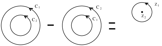
Figure 1: Diagrammatic representation of the contour manipulation needed to obtain the generalized (anti)commutation relations of the mode operators.

Making use of eqs. (3.12) and (3.10), the integral (3.11) can be computed for the class of contours considered. Obviously, we could apply the same procedure when the contour $C_{1}$ lies inside $C_{2}$. Notice that in this case the radial ordering reverses the order in which the fields are multiplied in (3.11). Actually, the radially ordered product can be computed by means of the relation (2.4). As shown in figure 1, the difference between the integrals (3.11), evaluated for the two types of contours described above, gives rise to an integral in which $z_{1}$ is integrated along a small contour centered around $z_{2}$. The value of this last integral can be obtained by making use of the parafermionic OPEs (2.22). The final result of the calculation is the following algebraic relation satisfied by the modes of $\psi_{{1\over 2}}$ and $\psi_{-{1\over 2}}$:

$$\sum_{r=0}^{+\infty}\,{\cal D}_{-{2k+1\over 2k}}^{(r)}\, \Bigl{[}\,B^{(+)}_{{l-1\over 2k}\,+\,n-r-1}\,\,B^{(-)}_{-{l\over 2k}\,+\,m+r+1}\,\,-\,\,B^{(-)}_{-{l+1\over 2k}\,+\,m-r}\,\,B^{(+)}_{{l\over 2k}\,+\,n+r}\,\,\Bigr{]}\,=\,$$ (3.14)

$$=\,{1\over 2}\,(\,{l\over 2k}\,+\,n\,)\,\,(\,{l\over 2k}\,+\,n\,-\,1\,)\,\delta_{n+m,0}\,+\,{\cal O}^{({1\over 2})}_{n+m}\,\,.$$

Similarly, we could get the relation verified by the modes of $\psi_{1}$ and $\psi_{-1}$. The result is:

$$\sum_{r=0}^{+\infty}\,{\cal D}_{-{k+2\over k}}^{(r)}\, \Bigl{[}\,A^{(+)}_{{l-2\over k}\,+\,n-r-1}\,\,A^{(-)}_{-{l\over k}\,+\,m+r+1}\,\,+\,\,A^{(-)}_{-{l+2\over k}\,+\,m-r}\,\,A^{(+)}_{{l\over k}\,+\,n+r}\,\,\Bigr{]}\,=\,$$ (3.15)

$$=\,{1\over 2}\,(\,{l\over k}\,+\,n\,)\,\,(\,{l\over k}\,+\,n\,-\,1\,)\,\delta_{n+m,0}\,+\,{\cal O}^{(1)}_{n+m}\,\,.$$

In eqs. (3.14) and (3.15), ${\cal O}^{({1\over 2})}_{n}$ and ${\cal O}^{(1)}_{n}$ are the modes of the operators appearing on the right-hand side of eq. (2.22), namely:

$${\cal O}^{(\alpha)}_{n}\,=\,\oint\,\,{dz\over 2\pi i}\,\,z^{n+1}\,{\cal O}^{(\alpha)}(z)\,\,,\,\,\,\,\,\,\,\,\,\,\,\,\,\,\,\,\,\,\,\,\,\,\,\,\,\,\,\,\,\,\,\,\,\,\,\,\,\,\,\,\,\,\alpha\,=\,{1\over 2}\,,\,1\,.$$ (3.16)

Before extracting some consequences from eqs. (3.14) and (3.15), let us write down some other $Z$-algebraic relations obtained by applying the technique just described. First of all, from the integrals:

$$\oint_{C_{1}}\,{dz_{1}\over 2\pi i}\,\oint_{C_{2}}\,{dz_{2}\over 2\pi i}\,\,R\,\Bigl{(}\,\psi_{\pm{1\over 2}}\,(z_{1})\,\psi_{\pm{1\over 2}}\,(z_{2})\,\Bigr{)}\,z_{1}^{\pm{l\over 2k}+n}\,\,z_{2}^{\pm{l\over 2k}+m}\,(\,z_{1}\,-\,z_{2}\,)^{{1\over 2k}}\,\,\phi_{(l,\bar{l})}(0)\,,$$ (3.17)

we get:

$$\sum_{r=0}^{+\infty}\,{\cal D}_{{1\over 2k}}^{(r)}\,\Bigl{[}\,B^{(\pm)}_{{1\pm l\over 2k}\,+\,n-r}\,\,B^{(\pm)}_{\pm{l\over 2k}\,+\,m+r}\,\,+\,\,B^{(\pm)}_{{1\pm l\over 2k}\,+\,m-r}\,\,B^{(\pm)}_{\pm{l\over 2k}\,+\,n+r}\,\,\Bigr{]}\,=\,\pm\,{1\over\sqrt{k}}\,A^{(\pm)}_{\pm{l\over k}\,+\,n+m}\,.$$ (3.18)

Similarly, if we consider the integrals:

$$\oint_{C_{1}}\,{dz_{1}\over 2\pi i}\,\oint_{C_{2}}\,{dz_{2}\over 2\pi i}\,\,R\,\Bigl{(}\,\psi_{\pm 1}\,(z_{1})\,\psi_{\mp{1\over 2}}\,(z_{2})\,\Bigr{)}\,z_{1}^{\pm{l\over k}+n}\,\,z_{2}^{\mp{l\over 2k}+m}\,(\,z_{1}\,-\,z_{2}\,)^{-{1\over k}}\,\,\phi_{(l,\bar{l})}(0)\,,$$ (3.19)

the following relation is obtained:

$$\sum_{r=0}^{+\infty}\,{\cal D}_{-{1\over k}}^{(r)}\,\Bigl{[}\,A^{(\pm)}_{-{1\mp l\over k}\,+\,n-r}\,\,B^{(\mp)}_{\mp{l\over 2k}\,+\,m+r}\,\,-\,\,B^{(\mp)}_{-{2\pm l\over 2k}\,+\,m-r}\,\,A^{(\pm)}_{\pm{l\over k}\,+\,n+r}\,\,\Bigr{]}\,=\,-{1\over\sqrt{k}}\,B^{(\pm)}_{\pm{l\over 2k}\,+\,n+m}\,.$$ (3.20)

Notice that, in order to evaluate the right-hand side of eqs. (3.18) and (3.20), the values of the structure constants (2.21) are needed.

The primary fields of the parafermionic algebra are those that satisfy a certain highest-weight condition. Let us denote them by $\Phi^{l,\bar{l}}_{l,\bar{l}}$, where $l$ and $\bar{l}$ refer respectively to the holomorphic and antiholomorphic quantum numbers. All the fields in the parafermionic module are obtained as descendants of the $\Phi^{l,\bar{l}}_{l,\bar{l}}$’s. The highest-weight conditions satisfied by $\Phi^{l,\bar{l}}_{l,\bar{l}}$ are:

$$B^{(+)}_{{l\over 2k}\,+\,n}\,\,\Phi^{l,\,\bar{l}}_{l,\,\bar{l}}\,=\,A^{(+)}_{{l\over k}\,+\,n}\,\,\Phi^{l,\,\bar{l}}_{l,\,\bar{l}}\,=\,0\,,\,\,\,\,\,\,\,\,\,\,\,\,\,\,\,\,\,\,\,\,\,\,\,\,\,\,\,\,\,\,\,\,\,\,\,\,\,\,\,\,n\geq 0\,,$$

$$B^{(-)}_{-{l\over 2k}\,+\,n\,+1}\,\,\Phi^{l,\,\bar{l}}_{l,\,\bar{l}}\,=\,A^{(-)}_{-{l\over k}\,+\,n\,+1}\,\,\Phi^{l,\,\bar{l}}_{l,\,\bar{l}}\,=\,0\,,\,\,\,\,\,\,\,\,\,\,\,\,\,\,\,\,\,\,\,\,n\geq 0\,,$$ (3.21)

together with analogous antiholomorphic relations. Notice that the requirement (3.21) implies that the dimensions of the fields belonging to the module constructed by acting on $\Phi^{l,\bar{l}}_{l,\bar{l}}$ with “creation” operators are bounded from below.

The algebraic relations (3.14) and (3.15) for $n=m=0$ determine the dimensions of the primary fields. Indeed, applying in this case eqs. (3.14) and (3.15) to $\Phi^{l,\bar{l}}_{l,\bar{l}}$, we see that the left-hand side of the resulting equations vanish as a consequence of the highest-weight conditions (3.21). Moreover, by subtracting these two equations we generate on the right-hand side the energy-momentum tensor due to eq. (2.23). Taking into account that the zero mode of the energy-momentum tensor acts diagonally on the field $\Phi^{l,\bar{l}}_{l,\bar{l}}$ and its eigenvalue is precisely the conformal dimension $h_{l}$ of $\Phi^{l,\bar{l}}_{l,\bar{l}}$, one gets:

$$h_{l}\,=\,{l(2k-3l)\over 4k(2k+3)}\,\,.$$ (3.22)

It will be argued in section 4 that, from the analysis of the three-point functions of the model, the values of the highest-weight charges are restricted to the range $l\leq k$. From now on in this section, we shall assume that $l$ satisfies this condition. It is important to notice that the dimensions $h_{l}$ in eq. (3.22) can become negative within this range of values of $l$ (recall that the theory we are dealing with is not unitary).

In the remaining of this section we shall suppress, for notational simplicity, the dependence of the fields on the antiholomorphic quantum numbers and so, for example, we shall write $\Phi_{l}^{l}$ instead of $\Phi^{l,\bar{l}}_{l,\bar{l}}$. All the fields in the parafermionic module can be obtained by applying the mode operators to $\Phi_{l}^{l}$. Let us determine the conformal dimensions of the fields generated in this way. First of all, we consider the fields

$$\Phi^{l}_{l+n}\,=\,B^{(+)}_{{l+n-1\over 2k}\,-1}\,\cdots\,B^{(+)}_{{l+1\over 2k}\,-1}\,B^{(+)}_{{l\over 2k}\,-1}\,\Phi^{l}_{l}\,,$$ (3.23)

where $n\geq 0\,\,,\,\,n\in{\rm Z}\kern-3.8pt{\rm Z}\kern 2.0pt$. Notice that $\Phi^{l}_{l+n}\,\in\,{\cal H}_{(\,l+n,\bar{l}\,)}$. The dimension of $\Phi^{l}_{l+n}$ can be computed from (3.9) and the result is:

$$h^{l}_{l+n}\,\equiv\,\Delta\,(\,\Phi^{l}_{l+n}\,)\,=\,h_{l}\,+\,{n\over 4k}\,(\,4k\,-\,2l\,-\,n\,)\,.$$ (3.24)

Similarly, we can define the fields $\Phi^{l}_{l-n}$:

$$\Phi^{l}_{l-n}\,=\,B^{(-)}_{-{l-n+1\over 2k}}\,\cdots\,B^{(-)}_{-{l-1\over 2k}\,}\,B^{(-)}_{-{l\over 2k}}\,\Phi^{l}_{l}\,,$$ (3.25)

where, again, $n$ is a non-negative integer and now $\Phi^{l}_{l-n}\,\in\,{\cal H}_{(\,l-n,\bar{l}\,)}$. The calculation of the conformal weight in this case gives:

$$h^{l}_{l-n}\,\equiv\,\Delta\,(\,\Phi^{l}_{l-n}\,)\,=\,h_{l}\,+\,{n\over 4k}\,(\,2l\,-\,n\,)\,.$$ (3.26)

In a parafermionic highest-weight module the descendant fields have dimensions which, in general, do not differ by an integer. Actually, in our case, the fields whose conformal weights have different fractional part belong to a finite subset, which can be selected by restricting appropriately the range of values of the charge. Indeed, let $h_{m}^{l}$ be the dimension of $\Phi^{l}_{m}$. For $m\geq l$ ($m\leq l$), $h_{m}^{l}$ is given by eq. (3.24) (eq. (3.26) respectively). In principle, $m$ can be any integer. However, it is easy to verify from eqs. (3.24) and (3.26) that:

$$h_{m+2k}^{l} = h_{m}^{l}\,+\,k-m\,,\,\,\,\,\,\,\,\,\,\,\,\,\,\,\,\,\,\,m\geq l\,,$$

$$h_{m-2k}^{l} = h_{m}^{l}\,+\,m-k\,,\,\,\,\,\,\,\,\,\,\,\,\,\,\,\,\,\,\,m\leq l\,,$$ (3.27)

i.e. shifting the charge by $2k$ ($-2k$) in eq. (3.24) (eq. (3.26)), the corresponding dimension is shifted by an integer. Therefore, in the determination of the values of $h_{m}^{l}$ modulo ${\rm Z}\kern-3.8pt{\rm Z}\kern 2.0pt$, we can restrict $m$ to the range $l-2k\leq m\leq 2k+l$. Actually, the upper limit of the previous interval can be refined, since it is straightforward to check from eqs. (3.24) and (3.26) that:

$$h_{2k+l-r}^{l}\,=\,h^{l}_{l-r}\,+\,k-l\,,\,\,\,\,\,\,\,\,\,\,\,\,\,\,\,\,\,\,0\leq r\leq 2l\,.$$ (3.28)

Eq. (3.28) implies that we can take $l-2k\leq m\leq 2k-l$. Moreover, the values of $h_{m}^{l}$ for $l-2k\leq m\leq-l$ differ by an integer from the $h_{m}^{l}$’s for $l\leq m\leq 2k-l$, namely:

$$h_{-l-r}^{l}=h_{2k-l-r}^{l}\,+\,l-k\,,\,\,\,\,\,\,\,\,\,\,\,\,\,\,\,\,\,\,\,\,\,\,\,\,\,\,\,\,\,0\leq r\leq 2k-2l\,.$$ (3.29)

Taken together, eqs. (3.27)-(3.29) imply that $m$ can be restricted to the range $-l\leq m\leq 2k-l$ with $m-l\in{\rm Z}\kern-3.8pt{\rm Z}\kern 2.0pt$. The corresponding dimensions can be written as:

$$h^{l}_{m}\,=\,\cases{h_{l}\,+\,{(l-m)(l+m)\over 4k}&if $-l\,\leq\,m\leq\,l$\cr\cr h_{l}\,+\,{(m-l)(4k-l-m)\over 4k}&if $l\,<\,m\leq\,2k-l$.}$$ (3.30)

The analysis we have just done shows that all the fields obtained by acting with the mode operators on $\Phi_{l}^{l}$ have dimensions that differ by integers from the values written in eq. (3.30). Let us now define:

$$\hat{h}^{l}_{m}\,=\,{l(l+1)\over 2(2k+3)}\,-\,{m^{2}\over 4k}\,.$$ (3.31)

Then eq. (3.30) can be put as:

$$h^{l}_{m}\,=\,\cases{\hat{h}^{l}_{m}&if $-l\,\leq\,m\leq\,l$\cr\cr\hat{h}^{l}_{m}\,+\,m-l&if $l\,<\,m\leq\,2k-l$.}$$ (3.32)

In next section we shall interpret $\hat{h}^{l}_{m}$ in terms of the primary fields of the osp$(1|2)$ current algebra. This interpretation, together with eq. (3.32), will allow us to give an explicit free field representation of the operators $\Phi_{m}^{l}$, which, making use of the results of ref. [17], can be used to compute the correlation functions of the parafermionic theory.

4 Free Field Representation

In order to find an explicit free field realization of the graded parafermionic symmetry, let us consider again its realization in the osp$(1|2)/U(1)$ coset CFT. According to eq. (2.16), the generating parafermions $\psi_{\pm 1}$ and $\psi_{\pm{1\over 2}}$ are obtained by extracting the Cartan dependence from the osp$(1|2)$ currents. This factorization can be neatly done in the framework of a free field realization of the osp$(1|2)$ CFT, such as the one proposed in ref. [16] and further developed in refs. [17, 19]. Indeed, after some redefinitions of the fields considered in ref. [17], one can put the osp$(1|2)$ currents in the form given in eq. (2.16). The parafermionic currents are realized in terms of two scalar fields $\varphi_{1}$ and $\varphi_{2}$ and a pair of conjugate anticommuting ghost fields $\eta$ and $\xi$. The scalar fields $\varphi_{1}$ and $\varphi_{2}$ are normalized in such a way that their OPE is given by:

$$\varphi_{i}(z)\,\varphi_{j}(w)\,=\,-\delta_{ij}\,{\rm log}\,(z-w)\,,$$ (4.1)

whereas the fields $\eta$ and $\xi$ satisfy:

$$\eta(z)\,\xi(w)\,=\,\xi(z)\,\eta(w)\,=\,{1\over z-w}\,\,,$$ (4.2)

and their dimensions are:

$$\Delta(\eta)\,=\,1\,,\,\,\,\,\,\,\,\,\,\,\,\,\,\,\,\,\,\,\,\,\,\,\Delta(\xi)\,=\,0\,.$$ (4.3)

In terms of the free fields, the energy-momentum tensor $T$ can be obtained, through the Sugawara construction, as in eqs. (2.17) and (2.18). Its explicit expression is:

$$T\,=\,-{1\over 2}\,(\partial\varphi_{1})^{2}\,-{1\over 2}\,(\partial\varphi_{2})^{2}\,-\,{i\over 2\sqrt{2k+3}}\,\partial^{2}\,\varphi_{2}\,-\,\eta\partial\xi\,.$$ (4.4)

It is a simple exercise to check that the central charge obtained from eq. (4.4) coincides with the one written in eq. (2.20). Moreover, in terms of $\varphi_{1}$, $\varphi_{2}$, $\eta$ and $\xi$, the basic parafermionic currents $\psi_{\pm 1}$ and $\psi_{\pm{1\over 2}}$ are given by:

$$\psi_{1}\, = \,\Bigl{[}\,{1\over\sqrt{2}}\,\partial\varphi_{1}\,+\,{i\over 2}\,\sqrt{{2k+3\over k}}\,\partial\varphi_{2}\,+{1\over 2\sqrt{k}}\,\eta\xi\,\Bigr{]}\,e^{\sqrt{{2\over k}}\varphi_{1}}\,,$$

$$\psi_{{1\over 2}}\, = \,\Bigl{[}\,\bigl{(}\,{1\over 2}\,\partial\varphi_{1}\,+\,{i\over 2}\,\sqrt{{2k+3\over 2k}}\,\partial\varphi_{2}\,\bigr{)}\,\xi\,-\,{1\over 2\sqrt{2k}}\,\partial\xi\,+\,{1\over\sqrt{2k}}\,\eta\,\Bigr{]}\,e^{{1\over\sqrt{2k}}\varphi_{1}}\,,$$

$$\psi_{-{1\over 2}}\, = \,\Bigl{[}\,\bigl{(}\,-{1\over 2}\,\partial\varphi_{1}\,+\,{i\over 2}\,\sqrt{{2k+3\over 2k}}\,\partial\varphi_{2}\,\bigr{)}\,\xi\,+\,{4k+3\over 2\sqrt{2k}}\,\partial\xi\,-\,{1\over\sqrt{2k}}\,\eta\,\Bigr{]}\,e^{-{1\over\sqrt{2k}}\varphi_{1}}\,,$$

$$\psi_{-1}\, = \,\Bigl{[}\,-{1\over\sqrt{2}}\,\partial\varphi_{1}\,+\,{i\over 2}\,\sqrt{{2k+3\over k}}\,\partial\varphi_{2}\,+{1\over 2\sqrt{k}}\,\eta\xi\,+{k+1\over\sqrt{k}}\,\xi\partial\xi\,\Bigr{]}\,e^{-\sqrt{{2\over k}}\varphi_{1}}\,.$$ (4.5)

The graded nature of the currents $\psi_{\pm 1}$ and $\psi_{\pm{1\over 2}}$ is manifest from their representation in eq. (4.5). After a short calculation it may be verified that $\psi_{\pm 1}$ and $\psi_{\pm{1\over 2}}$ are primary fields of the Virasoro algebra and that their dimensions are given by eq. (2.19). Moreover, it is easy to check that they indeed satisfy the parafermionic algebra of eq. (2.13) with the structure constants given by eq. (2.21). From the expressions given in eq. (4.5), one can generate all the other parafermionic currents of the model and get the structure constants of the algebra. This will be done in section 5.

The factorization of the Cartan degrees of freedom in the osp$(1|2)$ theory can also be performed on the primary fields of the model [17]. Let $G_{m}^{l}$ be an osp$(1|2)$ primary field corresponding to a value $l/2$ of the isospin and to a $H$-charge equal to $m/2$. According to the osp$(1|2)$ representation theory [14], the isospin of the finite-dimensional representations can take any positive integer or half-integer value and the difference between the Cartan eigenvalue and the isospin can be integer or half-integer. This implies that both $l$ and $m$ in $G_{m}^{l}$ are integers. Moreover [14], in an osp$(1|2)$ multiplet, $m$ can take values in the range $-l\leq m\leq l$. After extracting the Cartan dependence of $G_{m}^{l}$, one gets:

$$G_{m}^{l}\,=\,\Phi_{m}^{l}\,\,exp[\,i{m\over\sqrt{2k}}\,\,\varphi\,]\,,$$ (4.6)

where $\Phi_{m}^{l}$ is an operator which only depends on the fields of the osp$(1|2)/U(1)$ coset. The explicit expression of $\Phi_{m}^{l}$ for $-l\,\leq\,m\leq l$ is:

$$\Phi^{l}_{m}\,=\,\cases{exp\,[\,{m\over\sqrt{2k}}\,\,\varphi_{1}\,+\,{il\over\sqrt{2k+3}}\,\,\varphi_{2}\,]&if $l-m\in 2\,{\rm Z}\kern-3.8pt{\rm Z}\kern 2.0pt$\cr\cr\xi\,exp\,[\,{m\over\sqrt{2k}}\,\,\varphi_{1}\,+\,{il\over\sqrt{2k+3}}\,\varphi_{2}\,]&if $l-m\in 2\,{\rm Z}\kern-3.8pt{\rm Z}\kern 2.0pt\,+\,1\,$.}$$ (4.7)

Notice that the Grassmann character of $\Phi_{m}^{l}$ depends on whether $l-m$ is even or odd. From eqs. (4.7) and (4.4), it is immediate to find the conformal dimensions of the $\Phi_{m}^{l}$’s. The result of the calculation is:

$$\Delta(\,\Phi_{m}^{l}\,)\,=\,{l(l+1)\over 2(2k+3)}\,-\,{m^{2}\over 4k}\,=\,\hat{h}^{l}_{m}\,,$$ (4.8)

where $\hat{h}^{l}_{m}$ is the same as in eq. (3.31). In view of the result displayed in eq. (3.32), one is tempted to identify the fields (4.7) with the $\Phi_{m}^{l}$’s defined in eq. (3.25) for $-l\,\leq\,m\leq l$. Indeed, the operators (4.7) for $m=l$ verify the highest-weight conditions (3.21). Moreover, acting with the $\psi_{-{1\over 2}}$ current on the highest-weight field is equivalent, in the osp$(1|2)$ theory, to a multiplication by $j_{-}$ and, as shown in ref. [17], the different components of the $G_{m}^{l}$ operator are generated in this way. Alternatively, one can generate directly the form of the $\Phi_{m}^{l}$’s by using the explicit expressions of $\psi_{\pm{1\over 2}}$ and $\Phi_{l}^{l}$, given in eqs. (4.5) and (4.7) respectively. As the result of this calculation one can prove that, indeed, for $-l\,\leq\,m\leq l$, the expressions of $\Phi_{m}^{l}$ displayed in eq. (4.7) are recovered. For $m>l$ one obtains that $\Phi_{m}^{l}$ contains an exponential, such as the one in eq. (4.7), multiplied by a polynomial in the derivatives of the fields of dimension $m-l$. Notice that this representation of the $\Phi_{m}^{l}$’s for $m>l$ is in agreement with the dimensions written in eq. (3.32) for this case.

The relation (4.6) between operators of the osp$(1|2)$ and parafermionic theories allows one to express the correlation functions of the latter in terms of the vacuum expectation values of the former. Actually, from eq. (4.6) one obtains the following general result:

$$\langle\,\,\Phi_{m_{1},\bar{m}_{1}}^{l_{1},\bar{l}_{1}}\,(z_{1},\bar{z}_{1})\,\,\cdots\,\,\Phi_{m_{n},\bar{m}_{n}}^{l_{n},\bar{l}_{n}}\,(z_{n},\bar{z}_{n})\,\,\rangle\, = \,\prod_{i<j}^{n}\,(\,z_{i}\,-\,z_{j}\,)^{-{m_{i}m_{j}\over 2k}}\,(\,\bar{z}_{i}\,-\,\bar{z}_{j}\,)^{-{\bar{m}_{i}\bar{m}_{j}\over 2k}}\,\times$$

$$\times \langle\,\,G_{m_{1},\bar{m}_{1}}^{l_{1},\bar{l}_{1}}\,(z_{1},\bar{z}_{1})\,\,\cdots\,\,G_{m_{n},\bar{m}_{n}}^{l_{n},\bar{l}_{n}}\,(z_{n},\bar{z}_{n})\,\,\rangle\,.$$

As the Cartan degrees of freedom only contribute in eq. (LABEL:scinco) with factors which are powers of the coordinates, it is clear that the selection rules of the osp$(1|2)$ theory are inherited in the parafermionic model. These selection rules have been studied in detail in ref. [17]. Actually, by studying the operator product algebra of the osp$(1|2)$ CFT, it was demonstrated in ref. [17] that only those isospins lower or equal than $k/2$ are coupled ($k$ being the level of the osp$(1|2)$ Kac-Moody algebra). This result implies that, as was advanced around eq. (3.22), the charges $l$ of the highest-weight parafermionic fields $\Phi_{l}^{l}$ are restricted by the condition:

$$l\,\leq\,k\,.$$ (4.10)

Moreover, the analysis of ref. [17] can be used to get some highly non-trivial results in the parafermionic theory. Let us see, as an example, what is the value of the vacuum expectation value of the product of three highest-weight parafermionic fields. First of all, let us introduce the notation:

$${\cal S}_{l}\,\equiv\,\Phi_{l,l}^{l,l}\,,$$ (4.11)

and let the ${\cal S}_{l}$ fields be normalized in such a way that their two-point function is given by:

$$\langle\,\,{\cal S}_{l_{1}}\,(z_{1},\bar{z}_{1})\,\,{\cal S}_{l_{2}}^{\,\dagger}\,(z_{2},\bar{z}_{2})\,\,\rangle\,=\,\delta_{l_{1},l_{2}}\,\,|\,z_{1}\,-\,z_{2}\,|^{-4h_{l_{1}}}\,.$$ (4.12)

Then, on general grounds, we can write the non-vanishing correlator involving three operators of the type (4.11) as:

$$\langle\,\,{\cal S}_{l_{1}}\,(z_{1},\bar{z}_{1})\,\,{\cal S}_{l_{2}}\,(z_{2},\bar{z}_{2})\,\,{\cal S}_{l_{1}+l_{2}}^{\,\dagger}\,(z_{3},\bar{z}_{3})\,\,\rangle\, = \,{\cal C}_{l_{1},l_{2}}\,\,|\,z_{1}\,-\,z_{2}\,|^{2(\,h_{l_{1}+l_{2}}-h_{l_{1}}-h_{l_{2}}\,)}\,\,\times$$

$$\times \,|\,z_{1}\,-\,z_{3}\,|^{2(\,h_{l_{2}}-h_{l_{1}}-h_{l_{1}+l_{2}}\,)}\,\,|\,z_{2}\,-\,z_{3}\,|^{2(\,h_{l_{1}}-h_{l_{2}}-h_{l_{1}+l_{2}}\,)}\,,$$

where ${\cal C}_{l_{1},l_{2}}$ are constants whose value can be obtained from the three-point functions of the osp$(1|2)$ CFT. By using the results of ref. [17], one gets:

$$\bigl{[}\,{\cal C}_{l_{1},l_{2}}\,\bigr{]}^{2}\,\,=\,{\Gamma\Bigl{(}\,{k+2\over 2k+3}\,\Bigr{)}\over\Gamma\Bigl{(}\,{k+1\over 2k+3}\,\Bigr{)}}\,\,\,\,{\Gamma\Bigl{(}\,{k+2+l_{1}+l_{2}\over 2k+3}\,\Bigr{)}\,\,\Gamma\Bigl{(}\,{k+1-l_{1}\over 2k+3}\,\Bigr{)}\,\,\Gamma\Bigl{(}\,{k+1-l_{2}\over 2k+3}\,\Bigr{)}\over\Gamma\Bigl{(}\,{k+1-l_{1}-l_{2}\over 2k+3}\,\Bigr{)}\,\,\Gamma\Bigl{(}\,{k+2+l_{1}\over 2k+3}\,\Bigr{)}\,\,\Gamma\Bigl{(}\,{k+2+l_{2}\over 2k+3}\,\Bigr{)}}\,\,.$$ (4.14)

It is possible to realize the parafermionic algebra in terms of three scalar fields. This realization can be found by representing the $\eta$ and $\xi$ fields by means of a new scalar field $\varphi_{3}$:

$$\eta\,=\,e^{i\varphi_{3}}\,,\,\,\,\,\,\,\,\,\,\,\,\,\,\,\,\,\,\,\,\,\,\,\xi\,=\,e^{-i\varphi_{3}}\,.$$ (4.15)

It can be readily proved that $\eta$ and $\xi$, as given by eq. (4.15), do indeed satisfy the OPE (4.2) if $\varphi_{3}$ is normalized in such a way that eq. (4.1) also holds for $i,j=3$. Moreover, the energy-momentum tensor is:

$$T\,=\,-{1\over 2}\,(\partial\varphi_{1})^{2}\,-{1\over 2}\,(\partial\varphi_{2})^{2}\,-{1\over 2}\,(\partial\varphi_{3})^{2}\,-\,{i\over 2\sqrt{2k+3}}\,\partial^{2}\,\varphi_{2}\,-\,{i\over 2}\,\partial^{2}\,\varphi_{3}\,.$$ (4.16)

Making use of eq. (4.15), one can compute the normal ordered products involving the $\eta$ and $\xi$ fields which appear in the expression (4.5) of the parafermionic currents. After some algebra one finds the form of $\psi_{\pm 1}$ and $\psi_{\pm{1\over 2}}$ as a function of $\varphi_{1}$, $\varphi_{2}$ and $\varphi_{3}$:

$$\psi_{1}\, = \,\Bigl{[}\,{1\over\sqrt{2}}\,\partial\varphi_{1}\,+\,{i\over 2}\,\sqrt{{2k+3\over k}}\,\partial\varphi_{2}\,+\,{i\over 2\sqrt{k}}\,\partial\varphi_{3}\,\Bigr{]}\,e^{\sqrt{{2\over k}}\varphi_{1}}\,,$$

$$\psi_{{1\over 2}}\, = \,\Bigl{[}\,{1\over 2}\,\partial\varphi_{1}\,+\,{i\over 2}\,\sqrt{{2k+3\over 2k}}\,\partial\varphi_{2}\,+\,{i\over 2\sqrt{2k}}\,\partial\varphi_{3}\,\Bigr{]}\,e^{{1\over\sqrt{2k}}\varphi_{1}\,-\,i\varphi_{3}}\,+\,\,{1\over\sqrt{2k}}\,e^{{1\over\sqrt{2k}}\varphi_{1}\,+\,i\varphi_{3}}\,,$$

$$\psi_{-{1\over 2}}\, = \,\Bigl{[}\,-{1\over 2}\,\partial\varphi_{1}\,+\,{i\over 2}\,\sqrt{{2k+3\over 2k}}\,\partial\varphi_{2}\,-{i\over 2}\,{4k+3\over\sqrt{2k}}\,\partial\varphi_{3}\,\Bigr{]}\,e^{-{1\over\sqrt{2k}}\varphi_{1}\,-\,i\varphi_{3}}\,-\,{1\over\sqrt{2k}}\,e^{-{1\over\sqrt{2k}}\varphi_{1}\,+\,i\varphi_{3}}\,,$$

$$\psi_{-1}\, = \,\Bigl{[}\,-{1\over\sqrt{2}}\,\partial\varphi_{1}\,+\,{i\over 2}\,\sqrt{{2k+3\over k}}\,\partial\varphi_{2}\,+\,{i\over 2\sqrt{k}}\,\partial\varphi_{3}\,\Bigr{]}\,e^{-\sqrt{{2\over k}}\varphi_{1}}\,-\,{k+1\over\sqrt{k}}\,e^{-\sqrt{{2\over k}}\varphi_{1}-2i\varphi_{3}}\,.$$

Eq. (LABEL:sttres) will be particularly useful to obtain the expression of the $\psi_{l}$’s for $|l|\,>\,1$ and, as a consequence, to find the general form of the structure constants $C_{l,l^{\prime}}$, which characterize the graded parafermionic algebra (2.6). The determination of these constants will be the subject of section 5.

5 Structure Constants

Let us, first of all, introduce some machinery which we shall need later on in this section. We shall work in the fully bosonized representation of eq. (LABEL:sttres). In order to deal with compact expressions for the currents, we shall adopt a vector notation $\vec{\varphi}\,=\,(\,\varphi_{1},\varphi_{2},\varphi_{3}\,)$ for the fields. The following three-dimensional vectors:

$$\vec{A}\,=\,(\,\sqrt{{k\over 2}}\,,\,{i\over 2}\,\sqrt{2k+3}\,,\,{i\over 2}\,)\,,\,\,\,\,\,\,\,\,\,\,\,\,\,\,\,\,\,\,\,\vec{B}\,=\,(-\sqrt{{k\over 2}}\,,\,{i\over 2}\,\sqrt{2k+3}\,,\,{i\over 2}\,)\,,$$

$$\vec{a}\,=\,(\,\sqrt{{2\over k}}\,,\,0\,,\,0\,)\,,\,\,\,\,\,\,\,\,\,\,\,\,\,\,\,\,\,\,\,\,\,\,\,\,\,\,\,\,\,\,\,\,\,\,\,\,\,\,\,\,\,\,\,\,\,\,\,\vec{b}\,=\,(\,0\,,\,0\,,\,2i\,)\,,$$ (5.1)

will become relevant in our discussion. The components of $\vec{\varphi}$ along the vectors (5.1) will appear in our representation of the parafermionic currents.

The so-called Faá di Bruno (FdB) polynomials [20] are defined as:

$$P_{l}\,(\,\partial f\,)\,=\,e^{-f}\,\partial^{\,l}(\,e^{f}\,)\,,$$ (5.2)

where $f$ is a function and $l$ is a positive integer. Notice that the $P_{l}\,(\,\partial f\,)$’s are polynomials in the derivatives of $f$. The first FdB’s can be easily obtained from (5.2):

$$P_{0}\,=\,1\,,\,\,\,\,\,\,\,\,\,\,\,\,\,\,\,\,\,\,\,P_{1}\,=\,\partial f\,,\,\,\,\,\,\,\,\,\,\,\,\,\,\,\,\,\,\,\,P_{2}\,=\,(\,\partial f\,)^{2}\,+\,\partial^{2}\,f\,.$$ (5.3)

In general, these polynomials can be computed iteratively by using the relation:

$$P_{l+1}(\partial f)\,=\,\partial f\,P_{l}(\partial f)\,+\,\partial\,\Bigl{(}\,P_{l}(\partial f)\,\Bigr{)}\,,$$ (5.4)

which follows easily from eq. (5.2). The FdB polynomials play an important rôle in the theory of integrable hierarchies [21]. Their relevance in the free field representation of the parafermionic algebra was first pointed out in ref. [11]. In our case, we are going to argue that the general expression of the positively charged currents $\psi_{l}$ and $\psi_{l+{1\over 2}}$ with $l\in{\rm Z}\kern-3.8pt{\rm Z}\kern 2.0pt$ and $l\geq 0$ is given by:

$$\psi_{l}\, = \,{1\over N_{l}}\,P_{l}\,(\,\vec{A}\cdot\partial\vec{\varphi}\,)\,\,e^{\,l\vec{a}\cdot\vec{\varphi}}\,,$$

$$\psi_{l+{1\over 2}}\, = \,{1\over N_{l+{1\over 2}}}\,\Bigl{[}\,P_{l+1}\,(\,\vec{A}\cdot\partial\vec{\varphi}\,)\,\,e^{\,{1\over 2}\,[\,(2l+1)\vec{a}\,-\,\vec{b}\,]\,\cdot\,\vec{\varphi}}\,+\,\,P_{l}\,(\,\vec{A}\cdot\partial\vec{\varphi}\,)\,\,e^{\,{1\over 2}\,[\,(2l+1)\vec{a}\,+\,\vec{b}\,]\,\cdot\,\vec{\varphi}}\,\Bigr{]}\,,$$ (5.5)

$$\,\,\,\,\,\,\,\,\,\,\,\,\,\,\,\,\,\,\,\,\,\,\,\,\,\,\,\,\,\,\,\,\,\,\,\,\,\,\,\,\,\,\,\,\,\,\,\,\,\,\,\,\,\,\,\,\,\,\,\,(\,l\in{\rm Z}\kern-3.8pt{\rm Z}\kern 2.0pt\,\,,\,\,l\geq 0\,)$$

where $N_{l}$ and $N_{l+{1\over 2}}$ are normalization constants to be determined. We shall choose these constants to be positive. Indeed, the representation given in eq. (LABEL:sttres) for $\psi_{{1\over 2}}$ and $\psi_{1}$ coincides with the one in eq. (5.5) if we take $N_{1/2}\,=\,\sqrt{2k}$ and $N_{1}\,=\,\sqrt{k}$. In general, the form of the ansatz (5.5) can be inductively obtained by calculating the OPEs of the currents given in (5.5) with $\psi_{1}$ . Moreover, it is an easy exercise to verify that the dimensions of the operators (5.5) agree with the ones given in eq. (2.10).

The OPEs involving FdB polynomials and exponentials can be computed in a very systematic way. In appendix A we have detailed the general procedure that one must follow. In particular, the method of appendix A applied to the OPE of two positively charged parafermionic currents, represented as in eq. (5.5), leads to the result:

$$\psi_{l}(z)\,\psi_{l^{\prime}}(w)\, = \,(\,1\,+\,\epsilon(l)\,\epsilon(l^{\prime})\,)\,{N_{l+l^{\prime}}\over N_{l}\,N_{l^{\prime}}}\,\,{\psi_{l+l^{\prime}}(w)\over(z-w)^{{2ll^{\prime}\over k}\,+\,\epsilon(l)\,\epsilon(l^{\prime})}}\,+\,\cdots\,,$$ (5.6)

$$\,\,\,\,\,\,\,\,\,\,\,\,\,\,\,\,\,\,\,\,\,\,\,\,\,\,\,\,\,\,\,\,\,\,\,\,\,\,\,\,\,\,\,\,\,\,\,\,\,\,\,\,\,\,\,\,\,\,\,\,(\,l\,,\,\,l^{\prime}\geq 0\,)$$

where the function $\epsilon(l)$ has been defined in eq. (2.1). Eq. (5.6) does indeed confirm the correctness of our ansatz (5.5). Moreover, from eq. (5.6) we obtain the value of the structure constants for the products of two currents with positive charge in terms of the (up to now) unknown normalization constants $N_{l}$, namely:

$$C_{l,l^{\prime}}\,=\,(\,1\,+\,\epsilon(l)\,\epsilon(l^{\prime})\,)\,{N_{l+l^{\prime}}\over N_{l}\,N_{l^{\prime}}}\,\,,\,\,\,\,\,\,\,\,\,\,\,\,\,\,(\,l\,\,,\,\,l^{\prime}\geq 0\,)\,.$$ (5.7)

In order to determine the $C_{l,l^{\prime}}$’s (at least for $l,l^{\prime}\geq 0$), we must first know the $N_{l}$’s. These normalization constants are fixed by requiring the condition written down in eq. (2.14), which involves the currents with negative charge. In principle, the form of the $\psi_{-l}$’s for $l>0$ can be determined from the expression of $\psi_{-{1\over 2}}$ and $\psi_{-1}$ (see eq. (LABEL:sttres)). It turns out, however, that the expressions found are increasingly more complicated and it is far from obvious to get their general form. Let us illustrate this point with the first examples:

$$\psi_{-{1\over 2}}\, = \,{1\over N_{{1\over 2}}}\,\Bigl{[}\,[\,\vec{B}\,-\,(k+1)\,\vec{b}\,]\,\cdot\,\partial\vec{\varphi}\,\,e^{\,-{1\over 2}\,(\,\vec{a}\,+\,\vec{b}\,)\cdot\,\vec{\varphi}}\,\,-\,e^{\,-{1\over 2}\,(\,\vec{a}\,-\,\vec{b}\,)\,\cdot\,\vec{\varphi}}\,\Bigr{]}\,,$$

$$\psi_{-1}\, = \,{1\over N_{1}}\,\Bigl{[}\,\,\vec{B}\,\cdot\,\partial\vec{\varphi}\,\,e^{\,-\vec{a}\cdot\,\vec{\varphi}}\,\,-\,(k+1)\,e^{\,-(\vec{a}\,+\,\vec{b}\,)\,\cdot\,\vec{\varphi}}\,\Bigr{]}\,,$$

$$\psi_{-{3\over 2}}\, = \,{1\over N_{{3\over 2}}}\,\Bigl{[}\,[\,\vec{B}\,\cdot\partial\vec{\varphi}\,\vec{C}\,\cdot\partial\vec{\varphi}\,+\,\vec{B}\,\cdot\partial^{2}\vec{\varphi}\,-\,{1\over 2}\,(k+1)\,\vec{b}\,\cdot\partial^{2}\vec{\varphi}\,+$$

$$+ \,{1\over 2}\,(k+1)\,\vec{b}\,\cdot\partial\vec{\varphi}\,\vec{b}\,\cdot\partial\vec{\varphi}\,]\,e^{\,-{1\over 2}\,(\,3\vec{a}\,+\,\vec{b}\,)\,\cdot\,\vec{\varphi}}\,-\,\vec{B}\,\cdot\partial\vec{\varphi}\,e^{\,-{1\over 2}\,(\,3\vec{a}\,-\,\vec{b}\,)\,\,\cdot\,\vec{\varphi}}\,\,\,\Bigr{]}\,,$$

$$\psi_{-2}\, = \,{1\over N_{2}}\,\Bigl{[}\,[\,\vec{B}\,\cdot\partial\vec{\varphi}\,\vec{B}\,\cdot\partial\vec{\varphi}\,+\,\vec{B}\,\cdot\partial^{2}\vec{\varphi}\,]\,e^{\,-2\vec{a}\,\cdot\,\vec{\varphi}}\,-\,2(k+1)\,(\,\vec{B}\,-\vec{b})\cdot\partial\vec{\varphi}\,e^{\,-(2\vec{a}\,+\,\vec{b}\,)\cdot\,\vec{\varphi}}\,\,\,\Bigr{]}\,.$$

In eq. (LABEL:ouno) we have rewritten $\psi_{-{1\over 2}}$ and $\psi_{-1}$ in the more compact notation which makes use of the vectors (5.1). Of course, the different complexity of the parafermionic currents with positive and negative charge is an artifact of our particular free field realization. Indeed, one could represent the osp$(1|2)$ currents in such a way that the rôles of the positive and negative charges are interchanged and, as a consequence, the negatively charged parafermions would have a simple general form of the type given in eq. (5.5). The problem here is that, in order to normalize the currents as in eq. (2.14), we need to know the form of both types of currents. Fortunately, only some part of $\psi_{-l}$ contributes to the leading term of the normalization OPE. When $l$ is a positive integer, this part is easy to characterize. Indeed, the leading contribution to the right-hand side of eq. (2.14) is a c-number and, therefore, the only terms of the negatively charged currents that are relevant are the ones that have an exponential factor of the type $exp[-l\,\vec{a}\cdot\vec{\varphi}\,]$ (see eq. (5.5)). It is easy to see that for $l\in{\rm Z}\kern-3.8pt{\rm Z}\kern 2.0pt$ this type of term always appears in $\psi_{-l}$ and has the form:

$$\psi_{-l}\,=\,{1\over N_{l}}\,P_{l}(\,\vec{B}\cdot\partial\vec{\varphi}\,)\,e^{\,-l\vec{a}\,\cdot\,\vec{\varphi}}\,+\,\cdots\,\,,\,\,\,\,\,\,\,\,\,\,\,\,\,\,\,\,\,(\,l\in{\rm Z}\kern-3.8pt{\rm Z}\kern 2.0pt\,\,,\,\,l\geq 0\,)\,.$$ (5.9)

The presence of the term (5.9) in $\psi_{-l}$ can be verified in the expressions of $\psi_{-1}$ and $\psi_{-2}$ written in eq. (LABEL:ouno) and it is not hard to prove it in general. By applying the methods of appendix A, we can now compute the leading term of the OPE $\psi_{l}(z)\,\psi_{l^{\prime}}(w)$ and determine the value of $N_{l}$ for $l\in{\rm Z}\kern-3.8pt{\rm Z}\kern 2.0pt$. The result one arrives at is rather simple:

$$(\,N_{l}\,)^{2}\,=\,{k!\,l!\over(k-l)!}\,\,,\,\,\,\,\,\,\,\,\,\,\,\,\,\,\,\,\,(\,l\in{\rm Z}\kern-3.8pt{\rm Z}\kern 2.0pt\,\,,\,\,l\geq 0\,)\,.$$ (5.10)

If we knew the normalization constants $N_{l+{1\over 2}}$ for the half-integer currents, we would be able to write the general form of the $C_{l,l^{\prime}}$ constants for $l,l^{\prime}>0$. However, the direct calculation of $N_{l+{1\over 2}}$ is very difficult due to our failure in finding the general form of the term in $\psi_{-l-{1\over 2}}$ that contributes to its normalization. In the case of the structure constants $C_{l,l^{\prime}}$ that involve both positive and negative charges, the situation is even worse and only some particular cases can be computed directly. Some of these constants are:

$$C_{l,-{1\over 2}}\, = \,-l\,\,{N_{l-{1\over 2}}\over N_{l}\,N_{{1\over 2}}}\,,\,\,\,\,\,\,\,\,\,\,\,\,\,\,\,\,\,\,\,\,\,\,\,\,\,\,\,\,\,\,\,\,\,\,\,\,\,\,\,\,\,\,\,\,\,\,\,\,\,\,\,\,\,\,\,C_{l+{1\over 2},-{1\over 2}}\,=\,2(\,k-l\,)\,\,{N_{l}\over N_{l+{1\over 2}}\,N_{{1\over 2}}}\,,$$

$$C_{l,-1}\, = \,l(\,k-l+1\,)\,\,{N_{l-1}\over N_{l}\,N_{1}}\,,\,\,\,\,\,\,\,\,\,\,\,\,\,\,\,\,\,\,\,\,\,\,\,\,\,\,\,\,\,\,\,\,\,\,C_{l+{1\over 2},-1}\,=\,l(\,k-l\,)\,\,{N_{l-{1\over 2}}\over N_{l+{1\over 2}}\,N_{1}}\,.$$ (5.11)

$$\,\,\,\,\,\,\,\,\,\,\,\,\,\,\,\,\,\,\,\,\,\,\,\,\,\,\,\,\,\,\,\,\,\,\,\,\,\,\,\,\,\,\,\,\,\,\,\,\,\,\,(\,l\in{\rm Z}\kern-3.8pt{\rm Z}\kern 2.0pt\,\,,\,\,l\geq 0\,)$$

Remarkably, the knowledge of the explicit results (5.7), (5.10) and (5.11) is enough to obtain the full set of structure constants. Let us explain how this can be done by using the associativity condition of the parafermionic algebra. Let us consider the three-point correlator $\langle\,\psi_{m_{1}}(z_{1})\,\psi_{m_{2}}(z_{2})\,\psi_{m_{3}}(z_{3})\,\rangle$ which, due to charge conservation, is only non-vanishing if $m_{1}+m_{2}+m_{3}\,=\,0$. The dependence of this correlator on the coordinates is fixed by conformal invariance. This coordinate dependence can be compared with the one that is obtained by making use of the parafermionic OPEs (2.6). These OPEs can be computed in two different forms, that differ in the way in which we associate the currents. By comparing these two results with the exact value of the correlator, we obtain the following condition for the structure constants:

$$C_{m_{1},m_{2}+m_{3}}\,C_{m_{2},m_{3}}\,=\,C_{m_{1},m_{2}}\,C_{m_{1}+m_{2},m_{3}}\,\,,\,\,\,\,\,\,\,\,\,\,\,\,\,\,\,\,\,\,\,\,\,\,\,(\,m_{1}+m_{2}+m_{3}\,=\,0\,)\,.$$ (5.12)

Let us consider now eq. (5.12) for $m_{1}\,=\,l_{2}-l_{1}$, $m_{2}\,=\,l_{1}$ and $m_{3}\,=\,-l_{2}$ with $l_{1},l_{2}\geq 0$ and $l_{2}\geq l_{1}$. In this case, eq. (5.12) reduces to:

$$C_{l_{1},-l_{2}}\,=\,C_{l_{2}-l_{1},l_{1}}\,\,,\,\,\,\,\,\,\,\,\,\,\,\,\,\,\,\,\,\,(\,l_{2}\geq l_{1}\geq 0\,)\,.$$ (5.13)

In order to obtain eq. (5.13) we have taken into account that, according to eqs. (2.14) and (2.15), one has:

$$C_{l,-l}\,=\,(-1)^{\epsilon(l)}\,C_{-l,l}\,=\,1\,\,,\,\,\,\,\,\,\,\,\,\,\,\,\,\,\,\,\,\,(\,l\geq 0\,)\,.$$ (5.14)

Notice that eq. (5.13) relates some structure constants involving positive and negative charges to the $C_{l_{1},l_{2}}$’s for $l_{1},l_{2}\geq 0$. In particular, as $C_{l_{1},l_{2}}\,\geq\,0$ for $l_{1},l_{2}\geq 0$ (see eq. (5.7) and recall that the normalization constants are always positive), eq. (5.13) implies that $C_{l_{1},-l_{2}}\,\geq\,0$ for $l_{2}\geq l_{1}\geq 0$.

The condition (5.12) can be used to determine the behaviour of the structure constants $C_{l_{1},l_{2}}$ when the signs of both charges $l_{1}$ and $l_{2}$ are reversed. In general, due to the equivalence between the positive and negative charge sectors of the theory, $C_{l_{1},l_{2}}$ and $C_{-l_{1},-l_{2}}$ could differ at most by a sign. Accordingly, let us put:

$$C_{-l_{1},-l_{2}}\,=\,\sigma(l_{1},l_{2})\,C_{l_{1},l_{2}}\,,$$ (5.15)

where $\sigma(l_{1},l_{2})$ is a sign which can be determined by using the associativity condition. Indeed, let us take in eq. (5.12) $m_{1}\,=\,-l_{1}$, $m_{2}\,=\,-l_{2}$ and $m_{3}\,=\,l_{1}+l_{2}$, with $l_{1},l_{2}\geq 0$. Using again eq. (5.14), we get:

$$C_{-l_{1},-l_{2}}\,=\,(-1)^{\epsilon(l_{2})}\,C_{-l_{2},l_{1}+l_{2}}\,\,,\,\,\,\,\,\,\,\,\,\,\,\,\,\,\,\,\,\,(\,l_{1}\,,\,l_{2}\,\geq 0\,)\,,$$ (5.16)

which, after taking eqs. (5.13) and (5.15) into account, reduces to the following equation for $\sigma(l_{1},l_{2})$:

$$\sigma(l_{1},l_{2})\,=\,(-1)^{\epsilon(l_{2})}\sigma(l_{2},-l_{1}-l_{2})\,.$$ (5.17)

In order to solve eq. (5.17), we assume that $\sigma(l_{1},l_{2})$ only depends on the integer or half-integer nature of $l_{1}$ and $l_{2}$ and is a symmetric function of its arguments. Adopting the ansatz:

$$\sigma(l_{1},l_{2})\,=\,(-1)^{\alpha(\epsilon(l_{1})+\epsilon(l_{2}))\,+\,\beta\epsilon(l_{1})\epsilon(l_{2})}\,,$$ (5.18)

one easily gets that eq. (5.17) is solved if $\beta\,=\,\alpha-1$. This solution can be completely determined by looking at some particular cases of $l_{1}$ and $l_{2}$. So, for example, it is clear from eq. (2.21) that $\sigma(\,{1\over 2},{1\over 2}\,)\,=-1$ and $\sigma(\,1,-{1\over 2}\,)\,=\,+1$. These values are reproduced by our solution if $\alpha\,=\,0$. Thus, one has:

$$C_{-l_{1},-l_{2}}\,=\,(-1)^{\epsilon(l_{1})\epsilon(l_{2})}C_{l_{1},l_{2}}\,.$$ (5.19)

The behaviour of eq. (5.19) can be checked in some other particular cases in which the structure constants can be computed directly. This verification gives support to the hypothesis we have assumed in the derivation of eq. (5.19). On the other hand, notice that eq. (5.19) gives the structure constants involving two negative charges in terms of the constants for two positive charges. It is also possible to relate the constants $C_{l_{1},-l_{2}}$ for $l_{1}\,>l_{2}\,\geq\,0$ (i.e. the case not included in eq. (5.13)) to the constants given in eq. (5.7). This can be achieved by combining our previous relations. First of all, if $l_{1}\,>l_{2}\,\geq\,0$, eq. (2.15) allows one to write:

$$C_{l_{1},-l_{2}}\,=\,(-1)^{\epsilon(l_{2})}\,C_{-l_{2},l_{1}}\,\,,\,\,\,\,\,\,\,\,\,\,\,\,\,\,\,\,\,\,(\,l_{1}\,>l_{2}\,\geq\,0\,)\,.$$ (5.20)

Moreover, by using eq. (5.19) on the right-hand side of eq. (5.20), one arrives at:

$$C_{l_{1},-l_{2}}\,=\,(-1)^{\epsilon(l_{2})\,(\,\epsilon(l_{1})\,+\,1\,)}\,C_{l_{2},-l_{1}}\,\,,\,\,\,\,\,\,\,\,\,\,\,\,\,\,\,\,\,\,(\,l_{1}\,>l_{2}\,\geq\,0\,)\,.$$ (5.21)

Finally, by employing the relation (5.13), we can write:

$$C_{l_{1},-l_{2}}\,=\,(-1)^{\epsilon(l_{2})\,(\,\epsilon(l_{1})\,+\,1\,)}\,C_{l_{1}-l_{2},l_{2}}\,\,,\,\,\,\,\,\,\,\,\,\,\,\,\,\,\,\,\,(\,l_{1}>l_{2}\geq 0\,)\,.$$ (5.22)

Notice that the right-hand side of eq. (5.22) can be evaluated by means of eq. (5.7). Taken together, eqs. (5.13) and (5.22) give the structure constants for the product of a current of positive charge and a current of negative charge in terms of the $C_{l_{1},l_{2}}$’s with $l_{1},l_{2}\geq 0$. Let us write this result as:

$$C_{l_{1},-l_{2}}\,=\,\cases{C_{l_{2}-l_{1},l_{1}}&if $l_{2}\,\geq\,l_{1}\,\geq 0$\cr\cr(-1)^{\epsilon(l_{2})\,(\,\epsilon(l_{1})\,+\,1\,)}\,C_{l_{1}-l_{2},l_{2}}&if $l_{1}\,>\,l_{2}\,\geq 0\,.$}$$ (5.23)

Eqs. (5.23) and (5.19) reduce the problem of the determination of the structure constants to the evaluation of the right-hand side of eq. (5.7), i.e. to the calculation of the normalization constants $N_{l}$. Recall that we have found a partial answer to this problem (see eq. (5.10)). It remains to compute the normalization constants corresponding to the currents with half-integer charge. It turns out that the relations we have found allow one to express these constants in terms of the ones written in eq. (5.10). Let us, first of all, substitute in eq. (5.13) $l_{1}\,=\,{1\over 2}$ and $l_{2}=l$ with $l>0$. Eq. (5.13) reduces in this case to:

$$C_{{1\over 2},-l}\,=\,C_{l-{1\over 2},{1\over 2}}\,\,,\,\,\,\,\,\,\,\,\,\,\,\,\,\,\,\,\,(\,l>0\,\,,\,\,l\in{\rm Z}\kern-3.8pt{\rm Z}\kern 2.0pt\,)\,.$$ (5.24)

On the other hand, the right-hand side of eq. (5.24) can be computed by means of eq. (5.7) and the result is:

$$C_{l-{1\over 2},{1\over 2}}\,=\,2\,{N_{l}\over N_{l-{1\over 2}}\,N_{1\over 2}}\,\,,\,\,\,\,\,\,\,\,\,\,\,\,\,\,\,\,\,(\,l>0\,\,,\,\,l\in{\rm Z}\kern-3.8pt{\rm Z}\kern 2.0pt\,)\,,$$ (5.25)

whereas, after using eqs. (2.15) and (5.19), the constant appearing on the left-hand side of eq. (5.24) can be reduced to one of the cases of eq. (5.11), namely:

$$C_{{1\over 2},-l}\,=\,-C_{l,-{1\over 2}}\,=\,l\,{N_{l-{1\over 2}}\over N_{l}\,N_{{1\over 2}}}\,\,,\,\,\,\,\,\,\,\,\,\,\,\,\,\,\,\,\,(\,l>0\,\,,\,\,l\in{\rm Z}\kern-3.8pt{\rm Z}\kern 2.0pt\,)\,.$$ (5.26)

By substituting eqs. (5.25) and (5.26) in eq. (5.24), we find:

$$(\,N_{l-{1\over 2}}\,)^{2}\,=\,{2\over l}\,(\,N_{l}\,)^{2}\,\,,\,\,\,\,\,\,\,\,\,\,\,\,\,\,\,(\,l\in{\rm Z}\kern-3.8pt{\rm Z}\kern 2.0pt\,,\,l>0\,)\,,$$ (5.27)

which is the announced relation. From eqs. (5.10) and (5.27), we can write the general expression of $N_{l}$ for arbitrary $l$:

$$(\,N_{l}\,)^{2}\,=\,(\,1\,+\,\epsilon(l)\,)\,{k!\,[\,l\,]!\over[\,k-l\,]!}\,.$$ (5.28)

In eq. (5.28) the brackets denote integer part (as in eq. (2.2)). It is now immediate to find the structure constants. Indeed, after substituting eq. (5.28) on the right-hand side of eq. (5.7), we find the simple expression:

$$C_{l,l^{\prime}}^{2}\,=\,{[\,l\,+\,l^{\prime}\,]!\,[\,k\,-\,l\,]!\,[\,k\,-\,l^{\prime}\,]!\over k!\,[\,l\,]!\,[\,l^{\prime}\,]!\,[\,k\,-\,l\,-\,l^{\prime}\,]!}\,\,,\,\,\,\,\,\,\,\,\,\,\,\,\,\,\,\,\,\,\,\,\,\,\,\,\,\,\,\,\,\,(\,l\,,\,l^{\prime}\geq 0\,)\,.$$ (5.29)

Several remarks concerning eq. (5.29) are in order. First of all, it is worthwhile to point out that we must take the positive sign of the square root when computing $C_{l,l^{\prime}}$ from eq. (5.29) (recall that $C_{l,l^{\prime}}\,\geq\,0$ for $l,l^{\prime}\,\geq\,0$). Secondly, although eqs. (5.29), (5.23) and (5.19) have been obtained in an indirect way by means of a chain or arguments based on eq. (5.12), their predictions can be successfully compared with the results of direct calculations such as the ones written in eq. (5.11). Moreover, it is interesting to stress the differences and similarities between our result and the one corresponding to the $Z_{k}$ parafermions. It is clear from the comparison of eqs. (5.29), (5.23) and (5.19) and the values given in ref. [3] for the structure constants that, when the charges are integer, our results coincide with those of ref. [3]. Indeed, if $l,l^{\prime}\,\in{\rm Z}\kern-3.8pt{\rm Z}\kern 2.0pt$, one can eliminate the integer part symbol from the right-hand side of eq. (5.29) and, on the other hand, all minus signs in eqs. (5.19) and (5.23) and (2.15) disappear. On the contrary, when any of the charges is half-integer, our eq. (5.29) differs from the result of ref. [3] and minus signs, which reflect the graded nature of our system, do appear in some of the structure constants.

6 Concluding Remarks

In this paper we have formulated a graded generalization of the parafermionic symmetry. By means of simple first-principle arguments we have been able to determine the general form of the algebra and, in particular, the conformal dimensions of the parafermionic currents. The results of this general analysis allowed us to identify the graded parafermionic system with the osp$(1|2)/U(1)$ CFT. By using this identification we have been able to prove the existence of a graded extension of the parafermionic symmetry and, actually, we have found a free field realization. The central charge $c$ of the model can be easily obtained from its osp$(1|2)/U(1)$ representation. The fact that $c<0$ implies that the theory cannot be unitary.

The parafermionic Hilbert space can be represented as a direct sum of highest-weight modules. The modes of the currents satisfy generalized (anti)commutation relations on this Hilbert space which determine the conformal dimensions of the operators of the field space of the model. The free field representation of our system can be used to obtain the structure constants of the current algebra, a highly non-trivial result which is a generalization of the one in ref. [3].

The ordinary parafermions were introduced in ref. [3] as a generalization of the Ising model and, in general, they describe self-dual critical points in $Z_{k}$ statistical systems. It would be desirable to have a similar interpretation for the CFT constructed in this paper. Notice that, although our model is very similar to the $Z_{k}$ parafermionic system, there exist substantial differences between them. First of all, there is the unitarity issue. Secondly, the set of conformal weights written in eq. (3.30) and those corresponding to the $Z_{k}$ parafermions are very different as a consequence of the different definitions of the highest-weight modules. Indeed, in our case, the highest-weight conditions (3.21) involve both the bosonic $A^{(\pm)}$ and the fermionic $B^{(\pm)}$ mode operators, whereas, on the contrary, only the $A^{(\pm)}$’s are used to define the highest-weight primary fields of the $Z_{k}$ parafermionic theory. Despite these difficulties, our system displays many good properties from the representation theory point of view and, for this reason, we believe that the symmetry studied could be important in the characterization of some critical statistical mechanics models.

There are some other interesting aspects of the graded parafermionic system which were not considered here. Let us mention some of them. First of all, we could compute the characters of the theory which, according to its representation as an osp$(1|2)/U(1)$ coset, are nothing but string functions of the osp$(1|2)$ affine superalgebra [22]. In the framework of the free field realization we could, in principle, develop a BRST formalism for the study of these characters, similar to the one constructed in ref. [12] for the $su(2)$ case. Moreover, one could analyze more general coset constructions involving the osp$(1|2)$ superalgebra. The parafermionic theory we have studied in this paper is just a particular example of these coset theories. However, in analogy with what happens in the $su(2)$ case, it might be that the graded parafermions are the building blocks of the osp$(1|2)$ coset models. Finally, it would be important to find out if the osp$(1|2)$ parafermions admit integrable deformations, similar to the ones that the $su(2)$ theory has [23]. In case of affirmative answer we would find new families of massive integrable two-dimensional theories.

7 Acknowledgments

We are grateful to I. P. Ennes and J. L. Miramontes for useful discussions and a critical reading of the manuscript. This work was supported in part by DGICYT under grant PB96-0960, by CICYT under grant AEN96-1673 and by the European Union TMR grant ERBFMRXCT960012.

APPENDIX A

In this appendix we are going to develop a method which allows the computation of OPEs of FdB polynomials and exponentials in a rather systematic way. Let us consider two operators $O_{1}(\,z\,)$ and $O_{2}(\,w\,)$, which have the generic form:

$$O_{1}(\,z\,)\, = \,P_{l_{1}}\,(\,\vec{A}_{1}\,\cdot\,\partial\vec{\varphi}\,(\,z\,)\,)\,e^{\vec{a}_{1}\,\cdot\,\vec{\varphi}\,(\,z\,)}\,,$$

$$O_{2}(\,w\,)\, = \,P_{l_{2}}\,(\,\vec{A}_{2}\,\cdot\,\partial\vec{\varphi}\,(\,z\,)\,)\,e^{\vec{a}_{2}\,\cdot\,\vec{\varphi}\,(\,z\,)}\,,$$

where $P_{l_{1}}$ and $P_{l_{2}}$ are FdB polynomials (defined in eq. (5.2)) and $\vec{A}_{1}$, $\vec{A}_{2}$, $\vec{a}_{1}$ and $\vec{a}_{2}$ are constant vectors. Our aim is to give an expression of the OPE $O_{1}(\,z\,)\,O_{2}(\,w\,)$. Recall (see eq. (5.2)) that the FdB polynomials are defined through the derivative of an exponential. Let us start our calculation by carrying out a point-splitting procedure, which distinguishes the coordinates of the fields where the derivative acts from the others. Therefore, instead of the expressions (LABEL:apauno), we shall consider the following bilocal representation of $O_{1}$ and $O_{2}$:

$$O_{1}(\,z\,)\, = \,\partial_{z_{2}}^{l_{1}}\,\Bigl{[}\,e^{(\,\vec{a}_{1}\,-\,\vec{A}_{1}\,)\,\cdot\,\vec{\varphi}\,(\,z_{1}\,)\,+\,\vec{A}_{1}\,\cdot\,\vec{\varphi}\,(\,z_{2}\,)}\,\Bigr{]}\,,$$

$$O_{2}(\,w\,)\, = \,\partial_{w_{2}}^{l_{2}}\,\Bigl{[}\,e^{(\,\vec{a}_{2}\,-\,\vec{A}_{2}\,)\,\cdot\,\vec{\varphi}\,(\,w_{1}\,)\,+\,\vec{A}_{2}\,\cdot\,\vec{\varphi}\,(\,w_{2}\,)}\,\Bigr{]}\,.$$ (A.3)

In eq. (A.3) (and in what follows) it is implicitly understood that after the derivatives are performed one must take the coincidence limit $z_{1}\rightarrow z_{2}\rightarrow z$ and $w_{1}\rightarrow w_{2}\rightarrow w$ (although this limit will no be indicated explicitly). The obvious advantage of eq. (A.3) with respect to our original expressions (LABEL:apauno) is that the expansion of the product of two bilocal operators (A.3) reduces to the OPE (of the derivatives) of two exponentials. Actually, let $F(z,w)$ be the function:

$$F(z,w)\,=\,(\,z_{1}\,-\,w_{1}\,)^{\alpha_{11}}\,(\,z_{1}\,-\,w_{2}\,)^{\alpha_{12}}\,(\,z_{2}\,-\,w_{1}\,)^{\alpha_{21}}\,(\,z_{2}\,-\,w_{2}\,)^{\alpha_{22}}\,,$$ (A.4)

where the $\alpha_{ij}$’s are the following scalar products:

$$\alpha_{11}\, = \,-(\,\vec{a}_{1}\,-\,\vec{A}_{1}\,)\,\cdot\,(\,\vec{a}_{2}\,-\,\vec{A}_{2}\,)\,,\,\,\,\,\,\,\,\,\,\,\,\,\,\,\,\,\,\,\,\,\,\,\,\,\,\,\,\,\,\,\,\,\,\,\,\,\,\,\,\,\alpha_{12}\,=\,-(\,\vec{a}_{1}\,-\,\vec{A}_{1}\,)\,\cdot\,\vec{A}_{2}\,,$$

$$\alpha_{21}\, = -\vec{A}_{1}\,\cdot\,(\,\vec{a}_{2}\,-\,\vec{A}_{2}\,)\,,\,\,\,\,\,\,\,\,\,\,\,\,\,\,\,\,\,\,\,\,\,\,\,\,\,\,\,\,\,\,\,\,\,\,\,\,\,\,\,\,\,\,\,\,\,\,\,\,\,\,\,\,\,\,\,\,\,\,\,\,\,\,\,\alpha_{22}\,=\,-\vec{A}_{1}\,\cdot\,\vec{A}_{2}\,.$$

By using the well-known rules for the computation of OPEs of exponentials of scalar fields, we immediately get:

$$O_{1}(\,z\,)\,O_{2}(\,w\,)\,=\,\partial_{z_{2}}^{l_{1}}\,\,\partial_{w_{2}}^{l_{2}}\,\,\Bigl{[}\,F(z,w)\,e^{(\,\vec{a}_{1}\,-\,\vec{A}_{1}\,)\,\cdot\,\vec{\varphi}\,(\,z_{1}\,)\,+\,\vec{A}_{1}\,\cdot\,\vec{\varphi}\,(\,z_{2}\,)\,+\,(\,\vec{a}_{2}\,-\,\vec{A}_{2}\,)\,\cdot\,\vec{\varphi}\,(\,w_{1}\,)\,+\,\vec{A}_{2}\,\cdot\,\vec{\varphi}\,(\,w_{2}\,)}\,\Bigr{]}\,.$$

(A.6)

In order to get the final result we must evaluate the derivatives and then take the $z_{1}\rightarrow z_{2}\rightarrow z$ and $w_{1}\rightarrow w_{2}\rightarrow w$ limits. We shall use Leibnitz’s rule, which, for the $l^{{\rm th}}$ derivative of the product of two functions $f$ and $g$, can be written as:

$$\partial^{l}\,(\,f\,g\,)\,=\,\sum_{r=0}^{l}\,{l\choose r}\,\partial^{r}\,f\,\partial^{l-r}\,g\,.$$ (A.7)

Let us write the coincidence limit of the derivatives of the function $F$ as:

$$\partial_{z_{2}}^{r}\,\,\partial_{w_{2}}^{s}\Bigl{[}\,F(z,w)\,\,\Bigr{]}\,=\,{1\over(z-w)^{\vec{a}_{1}\,\cdot\,\vec{a}_{2}}}\,\,{a_{rs}\over(\,z\,-\,w\,)^{r+s}}\,,$$ (A.8)

where the $a_{rs}$ are c-numbers and the coordinate dependence is fixed by the exponents $\alpha_{ij}$ of eq. (LABEL:apacuatro). (Notice that the sum of the $\alpha_{ij}$’s is $-\vec{a}_{1}\,\cdot\,\vec{a}_{2}$). Making use of these results, we can write:

$$O_{1}(\,z\,)\,O_{2}(\,w\,)\, = \,{1\over(z-w)^{\vec{a}_{1}\,\cdot\,\vec{a}_{2}}}\,\,\sum_{r=0}^{l_{1}}\,\sum_{s=0}^{l_{2}}\,\,{l_{1}\choose r}\,{l_{2}\choose s}\,{a_{rs}\over(\,z\,-\,w\,)^{r+s}}\times$$

$$\times \,P_{l_{1}-r}\,(\,\vec{A}_{1}\,\cdot\,\partial\vec{\varphi}\,(\,z\,)\,)\,\,P_{l_{2}-s}\,(\,\vec{A}_{2}\,\cdot\,\partial\vec{\varphi}\,(\,w\,)\,)\,e^{\vec{a}_{1}\,\cdot\,\vec{\varphi}\,(\,z\,)\,+\,\vec{a}_{2}\,\cdot\,\vec{\varphi}\,(\,w\,)}\,.$$

In order to obtain eq. (LABEL:apaocho) it is essential to realize that the derivatives of the exponentials in eq. (A.6) can be organized again as FdB polynomials. In this way, we get on the right-hand side of eq. (LABEL:apaocho) products of operators of the same type as in eq. (LABEL:apauno). The constants $a_{rs}$ can be obtained by evaluating explicitly the derivatives of $F$. In view of the form of $F$ (eq. (A.4)), this calculation reduces to the computation of the derivatives of powers. One gets:

$$a_{rs}\,=\,(-1)^{s}\,\,\sum_{n=0}^{r}\,\,\sum_{m=0}^{s}\,\,{r\choose n}\,{s\choose m}\,{\Gamma(\,\alpha_{21}+1\,)\,\Gamma(\,\alpha_{12}+1\,)\,\Gamma(\,\alpha_{22}+1\,)\over\Gamma(\,\alpha_{21}-n+1)\,\Gamma(\,\alpha_{12}-m+1\,)\,\Gamma(\,\alpha_{22}+m+n-r-s+1\,)}\,.$$

(A.10)

Let us illustrate our method in the case of the expansion of the product of two currents $\psi_{l_{1}}(z)$ and $\psi_{l_{2}}(w)$, where $l_{1}$ and $l_{2}$ are positive integers. The free-field expression of the currents $\psi_{l_{1}}(z)$ and $\psi_{l_{2}}(w)$ is given in the first equation in (5.5). Apart from the normalization constants $N_{l_{1}}$ and $N_{l_{2}}$, $\psi_{l_{1}}(z)$ and $\psi_{l_{2}}(w)$ are of the form (LABEL:apauno) with:

$$\vec{A}_{1}\,=\,\vec{A}_{2}\,=\,\vec{A}\,,\,\,\,\,\,\,\,\,\,\,\,\,\,\,\,\vec{a}_{1}\,=\,l_{1}\,\vec{a}\,,\,\,\,\,\,\,\,\,\,\,\,\,\,\,\,\vec{a}_{2}\,=\,l_{2}\,\vec{a}\,,$$ (A.11)

where the vectors $\vec{A}$ and $\vec{a}$ have been defined in eq. (5.1). It is straightforward to compute the value of the scalar products $\alpha_{ij}$ in this case. The result is:

$$\alpha_{11}\, = l_{1}\,+\,l_{2}\,+1\,-\,{2l_{1}l_{2}\over k}\,,\,\,\,\,\,\,\,\,\,\,\,\,\,\,\,\,\,\,\,\,\,\,\,\,\,\,\,\,\,\,\,\,\,\,\,\,\,\,\,\,\alpha_{12}\,=\,-l_{1}-1\,,$$

$$\alpha_{21}\, = -l_{2}-1\,,\,\,\,\,\,\,\,\,\,\,\,\,\,\,\,\,\,\,\,\,\,\,\,\,\,\,\,\,\,\,\,\,\,\,\,\,\,\,\,\,\,\,\,\,\,\,\,\,\,\,\,\,\,\,\,\,\,\,\,\,\,\,\,\,\,\,\,\,\,\,\,\,\alpha_{22}\,=\,1\,.$$

Moreover, the sum (A.10), which gives the value of $a_{rs}$, can be easily obtained since it truncates. One gets:

$$a_{rs}\,=\,{(-1)^{r}\over l_{1}!l_{2}!}\,(\,l_{1}+s-1\,)!\,(\,l_{2}+r-1\,)!\,(\,l_{1}l_{2}-rs\,)\,.$$ (A.13)

Substituting eq. (A.13) in our general expression (LABEL:apaocho), we get:

$$\psi_{l_{1}}(z)\,\psi_{l_{2}}(w)\, = \,{1\over N_{l_{1}}N_{l_{2}}}\,{1\over(z-w)^{{2l_{1}l_{2}\over k}}}\,\sum_{r=0}^{l_{1}}\,\sum_{s=0}^{l_{2}}\,\,{l_{1}\choose r}\,{l_{2}\choose s}\,{(-1)^{r}\over l_{1}!l_{2}!}\,(\,l_{1}+s-1\,)!\,(\,l_{2}+r-1\,)!\,\times$$ (A.14)

$$\times\,{(\,l_{1}l_{2}-rs\,)\over(z-w)^{r+s}}\,\,P_{l_{1}-r}\,(\,\vec{A}\,\cdot\,\partial\vec{\varphi}\,(\,z\,)\,)\,\,P_{l_{2}-s}\,(\,\vec{A}\,\cdot\,\partial\vec{\varphi}\,(\,w\,)\,)\,e^{l_{1}\vec{a}\,\cdot\,\vec{\varphi}\,(\,z\,)\,+\,l_{2}\vec{a}\,\cdot\,\vec{\varphi}\,(\,w\,)}\,,$$

$$\,\,\,\,\,\,\,\,\,\,\,\,\,\,\,\,\,\,\,\,\,\,\,\,\,\,\,\,\,\,\,\,(\,l_{1}\,,\,l_{2}\,\geq 0\,\,\,\,\,l_{1}\,,\,l_{2}\,\in{\rm Z}\kern-3.8pt{\rm Z}\kern 2.0pt\,)$$

The right-hand side of eq. (A.14) should match the first equation in (2.13). It is clear that, in order to compare these two equations, we must expand in Taylor series the fields evaluated at $z$ on the right-hand side of eq. (A.14). A priori, it is not obvious that the leading singularity of the OPE (A.14) coincides with the one displayed in eq. (2.13). Actually, this coincidence only takes place if all the anomalous terms, present on the right-hand side of eq. (A.14), cancel. This cancelation is a highly non-trivial fact and is a consequence of the following identity satisfied by the FdB polynomials:

$$\sum_{r={\rm max}(0,p-l_{2})}^{l_{1}}\,\,\sum_{s={\rm max}(0,p-r)}^{l_{2}}\,\,{l_{1}\choose r}\,{l_{2}\choose s}\,{(-1)^{r}\over l_{1}!l_{2}!}\,(\,l_{1}+s-1\,)!\,(\,l_{2}+r-1\,)!\,\times$$

$$\times\,{(\,l_{1}l_{2}-rs\,)\over(r+s-p)!}\,\,\partial^{r+s-p}\,P_{l_{1}-r}\,(\,\vec{A}\,\cdot\,\partial\vec{\varphi}\,(\,w\,)\,)\,\,P_{l_{2}-s}\,(\,\vec{A}\,\cdot\,\partial\vec{\varphi}\,(\,w\,)\,)\,=\,$$

$$=\,\,\delta_{p,0}\,P_{l_{1}+l_{2}}\,(\,\vec{A}\,\cdot\,\partial\vec{\varphi}\,(\,w\,)\,)\,,\,\,\,\,\,\,\,\,\,\,\,\,\,\,\,\,\,\,\,\,\,\,\,\,\,\,\,\,\,\,\,\,(\,l_{1}\,,\,l_{2}\,\geq 0\,\,\,\,\,l_{1}\,,\,l_{2}\,\in{\rm Z}\kern-3.8pt{\rm Z}\kern 2.0pt\,)\,.$$ (A.15)

Eq. (A.15) can be verified by direct calculation (by making use of the explicit form of the FdB polynomials). Notice that the terms on the left-hand side of eq. (A.15) are precisely the ones generated when the FdB polynomials on the right-hand side of eq. (A.14) are expanded in Taylor series (i.e. one does not need to expand the exponential in order to cancel the anomalies). Therefore, the OPE of two currents can be written as:

$$\psi_{l_{1}}(z)\,\psi_{l_{2}}(w)\, = \,{1\over N_{l_{1}}N_{l_{2}}}\,\,{P_{l_{1}+l_{2}}\,(\,\vec{A}\,\cdot\,\partial\vec{\varphi}\,(\,w\,)\,)\,\,e^{(l_{1}+l_{2})\,\vec{a}\,\cdot\,\vec{\varphi}\,(\,w\,)\,}\over(z-w)^{{2l_{1}l_{2}\over k}}}\,+\,\cdots\,\,=$$ (A.16)

$$=\,{N_{l_{1}+l_{2}}\over N_{l_{1}}N_{l_{2}}}\,\psi_{l_{1}+l_{2}}\,(w)\,+\,\cdots\,,$$

$$\,\,\,\,\,\,\,\,\,\,\,\,\,\,\,\,\,\,\,\,\,\,\,\,\,\,\,\,\,\,\,\,(\,l_{1}\,,\,l_{2}\,\geq 0\,\,\,\,\,l_{1}\,,\,l_{2}\,\in{\rm Z}\kern-3.8pt{\rm Z}\kern 2.0pt\,)$$

a result which agrees with that written in eq. (5.6). In the case in which the charges $l_{1}$ and/or $l_{2}$ are positive half-integers, the corresponding OPEs can be computed in a similar way. In this case we must also use the second equation in (5.5). It can be checked that the anomaly cancelation also takes place in this case, again as a consequence of the identity (A.15). The general result of these OPEs has been written in eq. (5.6).

The method just described can also be employed to compute the normalization constants $N_{l}$ (see eq. (5.10)) and other structure constants (such as the ones in eq. (5.11)).

References

• [1] For a review see, for example, S. Ketov, “Conformal Field Theory”, (World Scientific, Singapore, 1995) and P. Di Francesco, P. Mathieu and D. Sénéchal, Conformal Field Theory, (Springer-Verlag, New York, 1997).
• [2] L. Kadanoff and H. Ceva, Phys. Rev. B3 (1971) 3918; E. Fradkin and L. Kadanoff, Nucl. Phys. B170 (1980)1.
• [3] A. B. Zamolodchikov and V. A. Fateev, Sov. Phys. JEPT 62 (1985) 215.
• [4] P. Goddard, A. Kent and D. Olive, Phys. Lett. B152 (1985) 88; Comm. Math. Phys. 103 (1986) 105.
• [5] D. Gepner, Nucl. Phys. B290 [FS20] (1987) 10.
• [6] A. B. Zamolodchikov and V. A. Fateev, Sov. Phys. JEPT 63 (1986) 913; Theor. Math. Phys. 71 (1987) 451.
• [7] D. Gepner and Z. Qiu, Nucl. Phys. B285 [FS19] (1987) 423.
• [8] J. Lykken, Nucl. Phys. B313 (1989) 473.
• [9] G. V. Dunne, I. G. Halliday and P. Suranyi, Nucl. Phys. B325 (1989) 526.
• [10] D. Nemeschansky, Nucl. Phys. B363 (1989) 665.
• [11] A. Bilal, Phys. Lett. B226 (1989) 272.
• [12] J. Distler and Z. Qiu, Nucl. Phys. B336 (1990) 533.
• [13] C. Ahn, S. Chung and S. H. Tye, Nucl. Phys. B365 (1991) 191.
• [14] A. Pais and V. Rittenberg, J. Math. Phys. 16 (1975) 2063; M. Scheunert, W. Nahm and V. Rittenberg, J. Math. Phys. 18 (1977) 155.
• [15] For a review on general aspects of Lie superalgebras see M. Scheunert, “The Theory of Lie Superalgebras”, Lect. Notes in Math. 716, (Springer-Verlag, Berlin, 1979) and L. Frappat, P. Sorba and A. Sciarrino, “Dictionary on Lie Superalgebras”, hep-th/9607161.
• [16] M. Bershadsky and H. Ooguri, Phys. Lett. B229 (1989) 374.
• [17] I. P. Ennes, A. V. Ramallo and J. M. Sánchez de Santos, Phys. Lett. B389 (1996) 485; Nucl. Phys. B491 [PM] (1997) 574.
• [18] I. P. Ennes and A. V. Ramallo, Nucl. Phys. B502 [PM] (1997) 671.
• [19] I. P. Ennes, P. Ramadevi, A. V. Ramallo and J. M. Sánchez de Santos, “Duality in osp$(1|2)$ Conformal Field Theory and link invariants”, hep-th/9709068 (in press in Int. J. Mod. Phys.).
• [20] M. Faá di Bruno, Quart. Jour. Pure Appl. Math. 1 (1857) 359.
• [21] see L. A. Dickey, “Soliton equations and Hamiltonian systems”, (World Scientific, Singapore, 1991).
• [22] V. Kac and D. Peterson, Adv. in Math. 53 (1984) 125.
• [23] V. A. Fateev, Int. J. Mod. Phys. A6 (1991) 2109.