DPNU-98-17

hep-th/9805035

May 1998

Abstract

A new formula for the composite Higgs boson mass is given, based on the Ward-Takahashi identity and the Schwinger-Dyson(SD) equation. In this formula the dominant asymptotic solution of the SD equation yields a correct answer, in sharp contrast to the Partially Conserved Dilatation Current(PCDC) approach where the sub- and sub-sub-dominant solutions should be taken into account carefully. In the gauged Nambu-Jona-Lasinio model we find $M_{H}\simeq\sqrt{2}M$ for the composite Higgs boson mass $M_{H}$ and the dynamical mass of the fermion $M$ in the case of the constant gauge coupling(with large cut off), which is consistent with the PCDC approach and the renormalization-group approach. As to the case of the running gauge coupling, we find $M_{H}\simeq 2\sqrt{(A-1)/(2A-1)}M$, where $A\equiv 18C_{2}/(11N_{c}-2N_{f})$ with $C_{2}$ being the quadratic Casimir of the fermion representation. We also discuss a straightforward application of our formula to QCD(without 4-Fermi coupling), which yields $M_{\sigma}\sim\sqrt{2}M_{dyn}$, with $M_{\sigma}$ and $M_{dyn}$ being the light scalar(“$\sigma$-meson”) mass and mass of the constituent quark, respectively.

The Nambu-Jona-Lasinio(NJL) model [1], which is not renormalizable in 4 dimensions, is familiar to us as an example of model for the dynamical symmetry breaking. The Gauged Nambu-Jona-Lasinio(GNJL) model has been studied vigorously [2, 3] and is known to be renormalizable in 4 dimensions [4]. Phenomenologically, it has been applied to the Top Mode Standard Model(TMSM) [5]. Unfortunately, however, it has been complicated to calculate the composite Higgs boson mass in this model by the approach based on the Schwinger-Dyson(SD) equation. Namely, the previous manner to estimate the composite Higgs boson mass [6] was based on the Partially Conserved Dilatation Current (PCDC) relation [7], where we needed inevitably to know the vacuum energy in the broken phase by way of the Cornwall-Jackiw-Tomboulis(CJT) potential [8]. The PCDC relation is [7]

$$M_{H}^{2}=-16\frac{d_{\theta}E}{d_{\sigma}^{2}f_{\pi}^{2}},$$ (1)

where $E$, $d_{\sigma}$ and $d_{\theta}$ are the vacuum energy, the scale dimension of $\sigma$ and that of the trace of the energy-momentum tensor, respectively. In the GNJL model, we know $d_{\theta}=2d_{\sigma}$ and $d_{\sigma}=2-\sqrt{1-\lambda/\lambda_{c}}$ [9], where $\lambda\equiv 3C_{2}\alpha/4\pi$ and $\lambda_{c}=1/4$, with $g$ and $C_{2}$ being the gauge coupling constant and the quadratic Casimir of the fundamental representation, respectively.

In this manner, the result based on the full non-linear SD equation yields $M_{H}\simeq\sqrt{2}M$ [6, 10], while the linearized solution does $M_{H}\simeq 2M$ for $\lambda\ll 1$ [6]. It implies that the usual bifurcation method [11] does not work in this method. Besides the SD approach, on the other hand, we can obtain the same result as that of the full non-linear one, $M_{H}\simeq\sqrt{2}M$, by the renormalization-group(RG) approach [12, 10]. In the RG approach, of course, we need not know the vacuum energy in the broken phase. Thus, it would be natural to seek another method without using the vacuum energy even in the SD approach.

In this paper, we derive a formula for the composite Higgs boson mass based on the Ward-Takahashi (WT) identity by using the technique of Ref. [13]. Then, we obtain analytically the same result as the RG approach in the case of the constant gauge coupling and new result for the running gauge coupling. Finally, we simply apply our method to the light scalar meson (“$\sigma$ meson”) in the QCD.

Let us consider the $SU(N_{c})$-gauged NJL model, with $U(1)_{L}\times U(1)_{R}$ chiral symmetry for simplicity:

$${\cal L} = \bar{\psi}(i\hbox to0.0pt{\hbox to5.30904pt{\hfil/\hfil}\hss}\partial-g\hbox to0.0pt{\hbox to7.50002pt{\hfil/\hfil}\hss}A)\psi+\frac{G}{2N_{c}}\left[(\bar{\psi}\psi)^{2}+(\bar{\psi}i\gamma_{5}\psi)^{2}\right]-\frac{1}{2}\mbox{tr}(F_{\mu\nu}F^{\mu\nu})$$ (2)

$$\to \bar{\psi}(i\hbox to0.0pt{\hbox to5.30904pt{\hfil/\hfil}\hss}\partial-g\hbox to0.0pt{\hbox to7.50002pt{\hfil/\hfil}\hss}A)\psi-\bar{\psi}(\sigma+i\gamma_{5}\pi)\psi-\frac{N_{c}}{2G}(\sigma^{2}+\pi^{2})-\frac{1}{2}\mbox{tr}(F_{\mu\nu}F^{\mu\nu}),$$ (3)

where we have used the auxiliary field method, $\sigma\propto\bar{\psi}\psi$ and $\pi\propto\bar{\psi}i\gamma_{5}\psi$, and $\psi$ belongs to the fundamental representation of $SU(N_{c})$, and $g$ and $G$ are the gauge coupling and the 4-Fermi coupling, respectively. Following Ref. [13], we consider the partition function including the source terms for the composite bosons from the beginning, which yields desired WT identities. Let us consider the following partition function:

$$Z[\eta,\bar{\eta},J_{A_{\mu}},J_{\sigma},J_{\pi}] \equiv \int{\cal D}\psi{\cal D}\bar{\psi}{\cal D}A_{\mu}{\cal D}\sigma{\cal D}\pi\exp\left(i\int dx^{4}{\cal L}+{\cal L}_{sourse}\right),$$ (4)

$${\cal L}_{sourse} \equiv \bar{\psi}\eta+\bar{\eta}\psi+J_{A_{\mu}}A_{\mu}+J_{\sigma}\sigma+J_{\pi}\pi.$$ (5)

Then, we easily obtain the chiral WT identity as follows:

$$\partial_{\mu}\langle\bar{\psi}\gamma^{\mu}\gamma_{5}\psi\rangle_{J}+i\langle\bar{\eta}\gamma_{5}\psi\rangle_{J}+i\langle\bar{\psi}\gamma_{5}\eta\rangle_{J}+2i\langle J_{\sigma}\pi\rangle_{J}-2i\langle J_{\pi}\sigma\rangle_{J}=0.$$ (6)

In the usual way, we define the effective action $\Gamma[\bar{\psi},\psi,A_{\mu},\sigma,\pi]$ by the Legendre transformation of $W[J]$, where $W[J]$ is the generating functional for the connected Green function $(iW[J]\equiv\ln Z[J])$. After we rewrite Eq. (6) in terms of $\Gamma[\bar{\psi},\psi,A_{\mu},\sigma,\pi]$, $\psi$, $\bar{\psi}$, $\sigma$ and $\pi$, we take the derivative with respect to $\psi$ and $\bar{\psi}$. By taking the Fourier transformation, we obtain the WT identity for the axial-vector vertex as follows:

$$q_{\mu}\Gamma_{5}^{\mu}(p+q,p) = iS_{f}^{-1}(p+q)\gamma_{5}+i\gamma_{5}S_{f}^{-1}(p)$$ (7)

$$-2\frac{\delta^{3}\Gamma[\bar{\psi},\psi,A_{\mu},\sigma,\pi]}{\delta\psi\delta\bar{\psi}\delta\sigma}(p+q,p)\pi(q)+2\frac{\delta^{3}\Gamma[\bar{\psi},\psi,A_{\mu},\sigma,\pi]}{\delta\psi\delta\bar{\psi}\delta\pi}(p+q,p)\sigma(q).$$

On the other hand, by definition of $f_{\pi}$, the decay constant of NG boson, it is well-known [14] that the following relation holds in the limit of $q^{\mu}\to 0$ :

$$q_{\mu}\Gamma_{5}^{\mu}(p+q,p)=iS_{f}^{-1}(p+q)\gamma_{5}+i\gamma_{5}S_{f}^{-1}(p)+\chi_{\pi}(p,q)f_{\pi}\qquad(q^{\mu}\to 0),$$ (8)

where $\Gamma_{5}^{\mu}(p+q,p)$ is the proper axial-vector vertex and $\chi_{\pi}(p,q)$ is the amputated Bethe-Salpeter(BS) amplitude defined by $\chi_{\pi}(p,q)\equiv S_{f}^{-1}(p+q){\cal F.T.}\langle 0|\mbox{T}\psi(x)\bar{\psi}(0)|\pi(q)\rangle S_{f}^{-1}(p)$. Comparing Eq. (7) with Eq. (8), we obtain

$$f_{\pi} = 2Z^{-1/2}_{\pi}(0)\langle\sigma\rangle,$$ (9)

$$\chi_{\pi}(p,0) = 2\gamma_{5}\frac{\Sigma(p)}{f_{\pi}},$$ (10)

where we used $iS_{f}^{-1}(p)\equiv\hbox to0.0pt{\hbox to5.03125pt{\hfil/\hfil}\hss}p-\Sigma(p)$ and $\langle\pi\rangle=0$ and $\pi=Z_{\pi}^{1/2}\pi_{R}$. Notice that in Eq. (7) the proper axial-vector vertex is directly obtained by the Legendre transformation.

In addition to these relations, we can derive the WT identity for the composite boson propagator by differentiating Eq. (6) with respect to $J_{\sigma}$ and $J_{\pi}$ :

$$\partial_{\mu}^{x}\langle\bar{\psi}(x)\gamma^{\mu}\gamma_{5}\psi(x)\sigma(y)\pi(z)\rangle_{J=0}+2i\langle\pi(x)\pi(z)\rangle_{J=0}\delta(x-y)-2i\langle\sigma(x)\sigma(y)\rangle_{J=0}\delta(x-z)=0.$$ (11)

After taking the Fourier transformation of (11), multiplying it by $\frac{\delta^{2}\Gamma[\bar{\psi},\psi,A_{\mu},\sigma,\pi]}{\delta\sigma\delta\sigma}$ and $\frac{\delta^{2}\Gamma[\bar{\psi},\psi,A_{\mu},\sigma,\pi]}{\delta\pi\delta\pi}$ and taking $q^{\mu}\to 0$ limit, we obtain the composite Higgs boson mass as

$$Z_{\sigma}^{-1}(0)M_{H}^{2}(0) = -\frac{Z_{\pi}^{1/2}(0)f_{\pi}}{2}\frac{\delta^{3}\Gamma[\bar{\psi},\psi,A_{\mu},\sigma,\pi]}{\delta\sigma\delta\pi\delta\pi}(0,0,0)$$ (12)

$$= -\langle\sigma\rangle\Gamma_{\sigma,\pi,\pi}(0,0,0),$$ (13)

where we used Eq. (9), and $Z_{\sigma}^{-1}(p)M_{H}^{2}(p)$ is defined through the $\sigma$-propagator $D_{\sigma}^{-1}(p)=\frac{\delta^{2}\Gamma[\bar{\psi},\psi,A_{\mu},\sigma,\pi]}{\delta\sigma\delta\sigma}(p)\equiv Z_{\sigma}^{-1}(p)(p^{2}-M_{H}^{2}(p))$ and $\Gamma_{\sigma,\pi,\pi}(0,0,0)\equiv\frac{\delta^{3}\Gamma[\bar{\psi},\psi,A_{\mu},\sigma,\pi]}{\delta\sigma\delta\pi\delta\pi}(0,0,0)$. Since Eq. (13) is derived through WT identity alone, Eq. (13) holds generally even in other models. In fact, we can easily confirm it in the linear-$\sigma$ model or the Standard Model(SM) at tree level. Thus, we may consider Eq. (13) as a generalization of the tree level relation in these models.

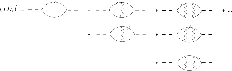
Figure 1: Insertion of $\sigma$ into the fermion propagator in the expression of the composite boson propagator $D_{\pi}^{-1}(0)$. The solid line, the doted external line, the wave line and the prime sign represent the full fermion propagator $S_{f}$, the composite boson $\pi$, the gluon propagator and insertion of $\sigma$ at zero momentum into the fermion propagator, respectively. Notice that insertion of $\sigma$ into the gluon propagator is in higher order of the $1/N_{c}$-expansion.

Now we come to evaluation of $\Gamma_{\sigma,\pi,\pi}(0,0,0)$. It is rather difficult to obtain non-perturbatively the 3-point vertex $\Gamma_{\sigma,\pi,\pi}(0,0,0)$ in general case. Fortunately, in the GNJL model we can easily estimate this 3-point vertex by using the non-perturbative propagator of $\pi$. The propagator of the composite boson in the GNJL model was obtained by Appelquist, Terning and Wijewardhana [15], whose technique was based on the resummation of the Taylor series around zero momentum of the composite boson under certain approximations. Recently, Gusynin and Reenders have given analytically the composite boson propagator in other approach without using the resummation [16]. As far as we discuss $\Gamma_{\sigma,\pi,\pi}(0,0,0)$, however, the resummation technique is enough. We obtain the 3-point vertex $\Gamma_{\sigma,\pi,\pi}(0,0,0)$ by insertion of $\sigma$ with zero momentum into the fermion propagator in the expression of $iD_{\pi}^{-1}(0)$, which consists of the ladder graphs, (see Fig. 1). Notice that insertion of $\sigma$ into the gluon propagator is similar to the vacuum polarization graph and is in higher-order of the $1/N_{c}$-expansion. By using the resummation technique, we find that $\Gamma_{\sigma,\pi,\pi}(0,0,0)$ is graphically equal to Fig. 2 at $1/N_{c}$-leading order.

Figure 2: The 3-point vertex $\Gamma_{\sigma,\pi,\pi}(0,0,0)$. The solid line with shaded blob and the doted external line represent the full fermion propagator $S_{f}$ and the composite bosons $\sigma,\pi$, respectively, while $\Gamma_{\sigma}$ and $\chi_{\pi}$ represent the $\sigma$-vertex ($\Gamma_{\sigma}(p)=\frac{d\Sigma(p)}{d\sigma}$ [4] ) and the $\pi$-vertex at zero momentum, respectively.

Thus, $\Gamma_{\sigma,\pi,\pi}(0,0,0)$ is written by

$$\Gamma_{\sigma,\pi,\pi}(0,0,0) = -2N_{c}Z_{\pi}^{-1}(0)\times$$ (14)

$$\int\frac{d^{4}p}{(2\pi)^{4}i}\mbox{tr}\left[\frac{1}{\hbox to0.0pt{\hbox to5.03125pt{\hfil/\hfil}\hss}p-\Sigma(p)}\frac{2\gamma_{5}\Sigma(p)}{f_{\pi}}\frac{1}{\hbox to0.0pt{\hbox to5.03125pt{\hfil/\hfil}\hss}p-\Sigma(p)}\frac{2\gamma_{5}\Sigma(p)}{f_{\pi}}\frac{1}{\hbox to0.0pt{\hbox to5.03125pt{\hfil/\hfil}\hss}p-\Sigma(p)}\frac{d\Sigma(p)}{d\sigma}\right]$$

$$= -2N_{c}Z_{\pi}^{-1}(0)\frac{1}{\pi^{2}}\int dxx\frac{\Sigma^{3}(x)\frac{d\Sigma(x)}{d\sigma}}{f_{\pi}^{2}(x+\Sigma^{2}(x))^{2}}\qquad(x=-p^{2}).$$ (15)

As is well-known, $f_{\pi}$ is estimated by the Pagels-Stokar(PS) formula [17]:

$$f_{\pi}^{2}=\frac{N_{c}}{2\pi^{2}}\int dxx\frac{\Sigma^{2}(x)-\frac{x}{4}\frac{d\Sigma^{2}(x)}{dx}}{(x+\Sigma^{2}(x))^{2}}.$$ (16)

Combining Eq. (13) with Eqs. (15) and (16), we finally obtain the formula for the composite Higgs boson mass as follows:

$$\frac{M_{H}^{2}}{4}=\int dxx\frac{\Sigma^{3}(x)\frac{d\Sigma(x)}{d\sigma}\langle\sigma\rangle}{(x+\Sigma^{2}(x))^{2}}\left/\int dxx\frac{\Sigma^{2}(x)-\frac{x}{4}\frac{d\Sigma^{2}(x)}{dx}}{(x+\Sigma^{2}(x))^{2}}\right.,$$ (17)

where we used $Z_{\pi}(0)\simeq Z_{\sigma}(0)$ up to ${\cal O}(M/\Lambda)$ due to the chiral symmetry and defined $M_{H}\equiv M_{H}(0)$. Of course, we can easily extend this result to the $SU(N_{f})_{L}\times SU(N_{f})_{R}$-symmetric GNJL model or TMSM. Note that Eq. (17) reproduces the well-known NJL result $M_{H}^{2}=4\sigma^{2}$ in the pure NJL limit($\Sigma(x)=\sigma$).

In the case of the constant gauge coupling, we know the solution of the SD equation with one gluon exchange graph as [3]

$$\Sigma(x) \simeq M\left(\frac{x}{M^{2}}\right)^{\frac{-1+\sqrt{1-\lambda/\lambda_{c}}}{2}},$$ (18)

$$\sigma = \Sigma(\Lambda^{2})+\Lambda^{2}\Sigma^{\prime}(\Lambda^{2}),$$ (19)

where the bifurcation method [11] is used and the infrared mass $M$ is defined by $\Sigma(M^{2})=M$. From Eqs. (18) and (19) the composite Higgs boson mass is obtained as

$$\frac{M_{H}^{2}}{2M^{2}}\simeq 1+\left(\frac{M^{2}}{\Lambda^{2}}\right)^{1-\sqrt{1-\lambda/\lambda_{c}}},$$ (20)

where we used $\frac{d\Sigma(x)}{d\sigma}\simeq(x/\Lambda^{2})^{\frac{-1+\sqrt{1-\lambda/\lambda_{c}}}{2}}$ [4] and assumed $M_{H}^{2}(0)\simeq M_{H}^{2}(M^{2})\simeq M_{H}^{2}(M_{H}^{2})$. Eq. (20) yields $M_{H}\simeq\sqrt{2}M$ in the limit of $\Lambda\to\infty(\lambda\neq 0)$, which is the same result as that obtained by Shuto, Tanabashi and Yamawaki through the PCDC relation [6]. Eq. (20) also agrees with the RG analysis [12, 10] for a small gauge coupling $(1-\sqrt{1-\lambda/\lambda_{c}}\simeq\frac{\lambda}{2\lambda_{c}})$. In Ref. [10], Carena and Wagner also obtained the same result as Eq. (20) by estimating the curvature of the effective potential in terms of the solution of the SD equation. However, both methods [6, 10] essentially depend on the sub- and sub-sub-dominant solutions in the asymptotic expansion of the SD equation. The coefficient of the dominant term is obtained uniquely in various linearized methods, like the bifurcation method, the manner of replacing the mass function in the denominator of the SD equation by a constant mass, i.e., ($x+\Sigma^{2}(x)\to x+m^{2}$) and the power expansion for the SD equation, etc.. On the other hand, coefficients of the sub-, or sub-sub-dominant term are quite different depending on the linearized methods. (Compare Ref. [4] with Ref. [10]). On the contrary, in our method the dominant solution of the SD equation already gives the desirable answer without using the sub- and sub-sub-dominant terms, and hence our formula (17) is more convenient than the previous ones.

In the case of the running coupling, the solution of the SD equation is [9]

$$\Sigma(x)\simeq M\left(\frac{\ln x/\Lambda_{QCD}^{2}}{\ln M^{2}/\Lambda_{QCD}^{2}}\right)^{-A/2},$$ (21)

where we used the usual improved ladder calculation [18] and $\sigma\simeq\Sigma(\Lambda^{2})$ and $A\equiv 18C_{2}/(11N_{c}-2N_{f})$. Thus, we can obtain the composite Higgs mass in the GNJL model as follows:

$$\frac{M_{H}^{2}}{2M^{2}}\simeq\frac{2(A-1)}{2A-1}\left(\ln M^{2}/\Lambda_{QCD}^{2}\right)^{A}\frac{\left(\ln M^{2}/\Lambda_{QCD}^{2}\right)^{-2A+1}-\left(\ln\Lambda^{2}/\Lambda_{QCD}^{2}\right)^{-2A+1}}{\left(\ln M^{2}/\Lambda_{QCD}^{2}\right)^{-A+1}-\left(\ln\Lambda^{2}/\Lambda_{QCD}^{2}\right)^{-A+1}}.$$ (22)

This result is also consistent with RGE analysis at $1/N_{c}$-leading order. In the limit of $\Lambda\to\infty$, Eq. (22) gives $M_{H}=2\sqrt{(A-1)/(2A-1)}M$, which coincides with $M_{H}\simeq\sqrt{2}M$ of Eq. (20) in the limit of $A\to\infty$ (non-running limit).

Even if we consider pure QCD, i.e., the pure gauge limit of the GNJL model(without 4-Fermi coupling), we can obtain the same relation as Eq. (17) by repeating the previous derivation of the WT identity for the bi-local fields $\sigma\propto\bar{\psi}\psi$ and $\pi^{a}\propto\bar{\psi}i\gamma_{5}T^{a}\psi$. The solution of the SD equation is obtained as follows [14]:

$$\Sigma(x)\simeq\frac{C}{x}\left(\ln x/\Lambda_{QCD}^{2}\right)^{A/2-1}\qquad(x\gg\Lambda_{QCD}^{2}),$$ (23)

where the coefficient of $C$ is equal to $M_{dyn}\mu^{2}(\ln\mu^{2}/\Lambda_{QCD}^{2})^{-A/2+1}$ under the condition of $M_{dyn}=\Sigma(\mu^{2})$ at the renormalization point $\mu$ and $M_{dyn}$ is the constituent quark mass $(M_{dyn}\sim 320\mbox{MeV})$. Now, we divide the integrations in Eq. (17) into the infrared part$(\int_{0}^{\mu^{2}})$ and the asymptotic one$(\int_{\mu^{2}}^{\Lambda^{2}})$ and define $I_{infra}+I$ for the integration of the numerator and $J_{infra}+J$ for that of the denominator, where $I/M_{dyn}^{4}$ and $J/M_{dyn}^{2}$ are numerically equal to 0.22 and 0.44 for $\mu=$ 1 GeV and $\Lambda_{QCD}\sim$ 200 MeV, respectively. Thus, we find that $J_{infra}$ gives the same order contributions as that of $J$ to the decay constant $f_{\pi}$ in contrast to the case of the GNJL model with a small gauge coupling. It is very difficult to estimate the infrared correction of $J_{infra}$ without assumptions. We simply assume that the mass function depends linearly on $x$ in the infrared region as $\Sigma(x)\simeq\frac{M_{dyn}-\Sigma(0)}{\mu^{2}}x+\Sigma(0)\quad(0\leq x\leq\mu^{2}).$ We find $\Sigma(0)\sim$ 100 MeV, provided that the PS formula including the correction of $J_{infra}$ gives $f_{\pi}=93$ MeV. Then, we obtain $M_{\sigma}^{2}\sim 2.1\times M_{dyn}^{2}$ by using Eq. (17). This result is not changed for $N_{f}=2\sim 5$.

In summary, a new formula for the composite Higgs boson mass (17) was derived from the WT identity. In the GNJL model, the dominant solution of the SD equation gives the desirable answer consistent with the previous calculations [6, 12, 10]. Thus, our method is more convenient than the manner based on the PCDC relation which depends on the sub- and sub-sub-dominant terms. By using the formula of Eq. (17), the same analytical result (20) as that from the RGE analysis was obtained easily in the case of the constant gauge coupling. If the running coupling effects are taken into account, the new relation of $M_{H}\simeq 2\sqrt{(A-1)/(2A-1)}M$ is obtained for the GNJL model in the SD approach.

Our approach may also be applied to QCD. By using our formula naively, we obtain the scalar meson mass as $M_{\sigma}\sim\sqrt{2}M_{dyn}$, i.e., around 500 MeV, where the decay constant is estimated by the PS formula. It is consistent with the light scalar $\sigma$ meson, whose mass is 400-1200 MeV in Particle Data Group [19] and is recently estimated to be 400-600 MeV [20]. Of course, $f_{\pi}$ may be estimated by other approach instead of the PS formula, for instance, by the ladder exact approach [21], which, however, would not change significantly the relation of $M_{\sigma}\sim\sqrt{2}M_{dyn}$ in QCD.

A problem would be to clarify the relation between our formula and the PCDC relation, both of which yield similar results at least numerically. Actually, our Higgs mass formula of Eq. (17) does not look like a simple modification of the PCDC relation of Eq. (1). This will be studied in future work.

The author is very grateful to K. Yamawaki for helpful discussions and reading this manuscript carefully. Thanks are also due to M. Sugiura and V. A. Miransky for discussions.

References

[1] Y. Nambu and G. Jona-Lasinio, Phys. Rev. 122 (1961)
345.
[2] W. A. Bardeen, C. N. Leung and S. T. Love,
Phys. Rev. Lett. 56 (1986) 1230;
C. N. Leung, S. T. Love and W. A. Bardeen, Nucl. Phys. B273
(1986) 649.
[3] K.-I. Kondo, H. Mino, and K. Yamawaki,
Phys. Rev. D39 (1989) 2430;
K. Yamawaki,
in Proc. Johns Hopkins Workshop on Current Problems in Particle
Theory 12, Baltimore, June 8-10, 1988,
edited by G. Domokos and S. Kovesi-Domokos
(World Scientific Pub. Co. , Singapore 1988);
T. Appelquist, M. Soldate, T. Takeuchi and L. C. R. Wijewardhana,
ibid..
[4] K.-I. Kondo, M. Tanabashi, and K. Yamawaki, Prog.
Theor. Phys. 89 (1993) 1249; M. Harada, Y. Kikukawa, T. Kugo,
and H. Nakano, Prog. Theor. Phys. 92 (1994) 1161.
[5] V. A. Miransky, M. Tanabashi and K. Yamawaki,
Phys. Lett. B221(1989)177 ; Mod. Phys. Lett. A4(1989)1043;
Y. Nambu, Enrico Fermi Institute Report No. 89-08, 1989
(unpublished); in Proceedings of the 1989 Workshop
on Dynamical Symmetry Breaking, edited by T. Muta and K. Yamawaki
(Nagoya University, Nagoya, Japan, 1990);
W. A. Bardeen, C. T. Hill, and M. Lindner, Phys. Rev. D41(1990)1647.
[6] S. Shuto, M. Tanabashi and K. Yamawaki, in
Proceedings of the 1989 Workshop on
Dynamical Symmetry Breaking, Nagoya, Dec. 21-23, 1989,
edited by T. Muta and K. Yamawaki
(Nagoya University, Nagoya, Japan, 1990).
[7] V. P. Gusynin and V. A. Miransky, Phys. Lett. B198
(1987) 79.
[8] J. M. Cornwall, R. Jackiw, and E. Tomboulis,
Phys. Rev. D10 (1974) 2428;
For a recent review, R. W. Haymaker, Riv. Nuovo Cim. 14 (1991) 1.
[9] V. A. Miransky and K. Yamawaki, Mod. Phys. Lett.
A4(1989)129.
[10] M. Carena and C. E. M. Wagner, Phys. Lett. B285 (1992) 277.
[11] D. Atkinson, J. Math. Phys. 28 (1987) 2494.
[12] W. A. Bardeen and S. T. Love, Preprint
FERMILAB-PUB-91/233-T.
[13] Shen Kun and Q. Zhongping, Phys. Rev. D45
(1992) 3877; K. Shen and Y. P. Kuang, Phys. Rev. D57 (1998) 6386.
[14] See, for example,
V. A. Miransky, Dynamical Symmetry Breaking
in Quantum Field Theories (World Scientific Pub. Co. , Singapore 1993).
[15] T. Appelquist, J. Terning and
L. C. R. Wijewardhana, Phys. Rev. D44 (1991) 871.
[16] V. P. Gusynin and M. Reenders, Phys. Rev. D57 (1998)
6356.
[17] H. Pagels and S. Stokar, Phys. Rev. D20 (1979) 2947.
[18] V. A. Miransky, Sov. J. Nucl. Phys. 38
(1983) 280; K. Higashijima, Phys. Rev. D29 (1984) 1228.
[19] Particle Data Group, Phys. Rev. D54 (1996) 1.
[20] M. Harada, F. Sannino and J. Schechter,
Phys. Rev. D54 (1996) 1991; S. Ishida, M. Ishida,
H. Takahashi, T. Ishida, K. Takamatsu and T. Tsuru,
Prog. Theor. Phys. 95 (1996) 745; S. Ishida, T. Ishida,
M. Ishida, K. Takamatsu and T. Tsuru,
Prog. Theor. Phys. 98 (1997) 1005; M. D. Scadron,
hep-ph/9710317; V. Elias, A. H. Fariborz, F. Shi and T. G. Steele,
Nucl. Phys. A633 (1998) 279.
[21] K.-I. Aoki, M. Bando, T. Kugo, M. G. Mitchard and
H. Nakatani, Prog. Theor. Phys. 84 (1990) 683;
T. Kugo and M. G. Mitchard, Phys. Lett. B286 (1992) 355.