We use a gauge-invariant regularization procedure, called split dimensional regularization, to evaluate the quark self-energy $\rm\Sigma(p)$ and quark-quark-gluon vertex function $\rm\Lambda_{\mu}(p^{\prime},p)$ in the Coulomb gauge, $\rm\vec{\bigtriangledown}\cdot\vec{A}^{a}=0$. The technique of split dimensional regularization was designed to regulate Coulomb-gauge Feynman integrals in non-Abelian theories. The technique which is based on two complex regulating parameters, $\omega$ and $\sigma$, is shown to generate a well-defined set of Coulomb-gauge integrals. A major component of this project deals with the evaluation of four-propagator and five-propagator Coulomb integrals, some of which are nonlocal. It is further argued that the standard one-loop BRST identity relating $\Sigma$ and $\Lambda_{\mu}$, should by rights be replaced by a more general BRST identity which contains two additional contributions from ghost vertex diagrams. Despite the appearance of nonlocal Coulomb integrals, both $\Sigma$ and $\Lambda_{\mu}$ are local functions which satisfy the appropriate BRST identity. Application of split dimensional regularization to two-loop energy integrals is briefly discussed.

Permanent address: On leave from the Department of Mathematics and Statistics, University of Guelph, Guelph, Ontario NIG 2W1.
E-mails: G.Leibbrandt@damtp.cam.ac.uk – mthgeorg@mail.cern.ch

CERN–TH/97–174

DAMTP–97–46

July 1997

1 Introduction

In our first test of the technique of split dimensional regularization, we evaluated the Yang-Mills self-energy to one loop and verified the appropriate BRST identity [1]. In this article, we present a second test of split dimensional regularization, also in the Coulomb gauge, by calculating the quark self-energy and quark-quark-gluon vertex functions. Our rationale for concentrating on one-loop calculations at this stage is very simple: we want to make sure that split dimensional regularization is capable of regulating unambiguously all one-loop integrals in the Coulomb gauge, before tackling the infamous divergences at two loops and beyond.

The Coulomb gauge has been highly successful in both electrostatics and quantum electrodynamics, especially in the treatment of bound-state problems [2]. By contrast, its application to non-Abelian models has been marred by the persistent appearance of ambiguous Coulomb-gauge Feynman integrals. It was Schwinger [3] who first noticed that the transition from a classical Hamiltonian to a quantum Hamiltonian led to instantaneous Coulomb-interaction terms. These terms, subsequently labelled $\rm V_{1}+V_{2}$-terms by Christ and Lee [4], are caused by the operator ordering problem, and arise whenever we convert a classical system to a quantum system. The principal problem with these new $\rm V_{1}+V_{2}$-terms is their nonlocality, foreshadowing potential difficulties in evaluating Feynman integrals.

A review of the historical development of the Coulomb gauge in the framework of Yang-Mills theory can be found in Ref. [2] and will not be repeated here. Suffice it to say, however, that the nonlocal $\rm V_{1}+V_{2}$-terms of Christ and Lee lead in general to momentum integrals containing two types of divergences: (a) ordinary UV divergences, related to the structure of space-time, and (b) new divergences, arising from the integration over the energy variable $\rm dq_{0}$, where $\rm d^{4}q\equiv dq_{0}~{}d^{3}\vec{q}$. Hence the name energy-integrals [5, 6]. It is the divergences from the energy-integrals that cause the notorious ambiguities in the Coulomb gauge, especially at two and three loops. To compound the issue, standard dimensional regularization is not powerful enough to consistently regulate the two types of infinities mentioned above, as first pointed out by Doust and Taylor [7, 8].

In 1996, we introduced a radically different method, called split dimensional regularization, for regulating Feynman integrals in the Coulomb gauge and applied it to the one-loop gluon self-energy $\rm\Pi^{ab}_{\mu\nu}$ [1, 9, 10]. The new technique employs two complex-dimensional parameters $\omega$ and $\sigma$, replacing the measure $\rm d^{4}q=dq_{0}~{}d^{3}\vec{q}$ by

$$\rm d^{2(\omega+\sigma)}q=d^{2\sigma}q_{0}~{}d^{2\omega}\vec{q}~{},$$ (1)

where the limits $\sigma\to(1/2)^{+}$, and $\omega\to(3/2)^{+}$ are to be taken after all integrations have been completed. Application of this procedure to the gluon self-energy $\rm\Pi^{ab}_{\mu\nu}(p)$ leads to the following results [1]:

• $\rm\Pi^{ab}_{\mu\nu}$ is local and nontransverse in the Coulomb gauge.

• Ghosts play a significant role, despite the physical nature of the Coulomb gauge.

• The BRST identity contains a nonvanishing ghost diagram, but is rigorously satisfied.

Encouraging as this initial result may be, it would be foolhardy to assume that split dimensional regularization can regulate not only the remaining one-loop integrals in the Coulomb gauge, but two- and three-loop integrals as well. After all, it is well known how annoyingly unpredictable noncovariant gauges may be at times! For this reason, we have decided to proceed with the investigation of one-loop diagrams, computing both the quark self-energy and quark-quark-gluon vertex function.
The latter is particularly challenging, since it contains for the first time, Coulomb-gauge integrals with five propagators.

The paper is organized as follows. In Section 2, we review the Feynman rules in the Coulomb gauge, and evaluate the quark self-energy $\Sigma$(p) using split dimensional regularization. The quark-quark-gluon vertex function $\rm\Lambda_{\mu}(p^{\prime},p)$ is calculated in Section 3. In Section 4, we illustrate the technique of split dimensional regularization for more complicated Coulomb-gauge integrals: for a massless four-propagator integral containing the instantaneous Coulomb-interaction propagators $\rm(\vec{q}^{2})^{-1}$ and $\rm[(\vec{q}+\vec{q})^{2}]^{-1}$, and for a massive five-propagator integral with propagators $\rm(\vec{q}^{2})^{-1}$ and $\rm[(\vec{q}-\vec{k})^{2}]^{-1}$. In Section 5, we examine the ghost contributions to the BRST identity and verify the latter. Implications of the technique of split dimensional regularization for two-loop energy integrals are discussed in Section 6. The highlights of our calculation are summarized in Section 7. The Appendix contains a partial list of integrals needed for the determination of $\Sigma$(p) and $\rm\Lambda_{\mu}(p^{\prime},p)$.

2 Feynman rules and computation of quark self-energy

2.1 Review of Feynman rules [11,12,13]

In Yang-Mills theory, with the Lagrangian density

$$\rm L^{\prime}=L-\frac{1}{2\alpha}({\it F}^{ab}_{\mu}A^{b\mu})^{2}~{},\alpha\equiv gauge~{}parameter,~{}\alpha\to 0~{},$$ (2)

where

$$F{\rm{}^{ab}_{\mu}}\!\! \equiv \!\!\rm(\partial_{\mu}-\frac{n\cdot\partial}{n^{2}}n_{\mu})\delta^{ab}~{},~{}~{}~{}~{}~{}\mu=0,1,2,3~{},$$

$$F{\rm{}^{ab}_{\mu}A^{\mu b}}\!\! = \!\!\rm\vec{\bigtriangledown}\cdot\vec{A}^{a}~{},~{}~{}~{}~{}~{}n_{\mu}\equiv(n_{0},\vec{n})=(1,\vec{0}),n^{2}=1~{},$$

$$\rm L\!\! = \!\!\rm-\frac{1}{4}(F^{a}_{\mu\nu})^{2}+(J^{c}_{\mu}+\bar{\omega}^{a}{\it F}^{ac}_{\mu})D^{cb\mu}\omega^{b}-\frac{1}{2}gf^{abc}K^{a}\omega^{b}\omega^{c}~{},$$

$$\rm F^{a}_{\mu\nu}\!\! = \!\!\rm\partial_{\mu}A^{a}_{\nu}-\partial_{\nu}A^{a}_{\mu}+gf^{abc}A^{b}_{\mu}A^{c}_{\nu}~{},$$

$$\rm D^{ab}_{\mu}\!\! = \!\!\rm\delta^{ab}\partial_{\mu}+gf^{abc}A^{c}_{\mu}~{},$$

the noncovariant Coulomb gauge is given by

$$\rm\vec{\bigtriangledown}\cdot\vec{A}^{a}(x)=0~{};$$ (3)

$\rm A^{a}_{\mu}$ is a massless gauge field, g the gauge coupling constant, $\rm f^{abc}$ are group structure constants, and $\rm a=1,...,N^{2}-1$, for SU(N); $\rm\omega^{a},\bar{\omega}^{a}$ represent ghost, anti-ghost fields respectively, while $\rm K^{a}$ and $\rm J^{a}_{\mu}$ denote external sources. The quantities $\rm J^{a}_{\mu},\omega^{a}$ and $\rm\bar{\omega}^{a}$ are anti-commuting.

In the Coulomb gauge, the Lagrangian density L^′ leads to the following gauge boson propagator [1]:

$$\rm G^{ab}_{\mu\nu}({\it q})=\frac{-i\delta^{ab}}{(2\pi)^{4}(q^{2}+i\varepsilon)}\left[g_{\mu\nu}-\left(\frac{n^{2}q_{\mu}q_{\nu}-q\cdot n(q_{\mu}n_{\nu}+q_{\nu}n_{\mu})}{-\vec{q}^{2}}\right)\right]~{},~{}~{}~{}~{}~{}\varepsilon>0~{},$$ (4)

while the three-gluon vertex is given by

$$\rm V^{abc}_{\mu\nu\rho}(p,{\it q},r)\!\! = \!\!\rm gf^{abc}(2\pi)^{4}\delta^{4}(p+q+r)[g_{\mu\nu}(p-q)_{\rho}$$ (5)

$$+ \!\!\rm g_{\nu\rho}(q-r)_{\mu}+g_{\rho\mu}(r-p)_{\nu}]~{},$$

and the scalar ghost propagator by

$$\rm G^{ab}_{ghost}=\frac{i\delta^{ab}}{(2\pi)^{4}\vec{q}^{2}}~{}.$$ (6)

2.2 Quark self-energy

The unintegrated expression for the quark self-energy in Minkowski space reads (cf. Fig. 1)

$$\rm\Sigma^{Coul}(p)\!\! = \!\!\rm\frac{4ig^{2}}{3}\int\frac{d^{4}q}{(2\pi)^{4}(q^{2}+i\varepsilon)}\gamma_{\nu}\frac{1}{(\not{p}-\not{\it q}-m+i\varepsilon)}\gamma_{\mu}$$ (7)

$$\!\!\rm\left[g^{\mu\nu}-\left(\frac{n^{2}q^{\mu}q^{\nu}-q\cdot n(q^{\mu}n^{\nu}+q^{\nu}n^{\mu})}{-\vec{\it q}^{2}}\right)\right],~{}n_{\mu}=(1,0,0,0),\varepsilon>0~{},$$

where m is the quark mass; the generators $\rm T^{a}_{\alpha\beta}$ have already been multiplied out. Expression (7) leads to trivial covariant integrals, and to noncovariant Coulomb-gauge integrals involving the factor $\rm 1/\vec{q}^{2}$. By performing a Wick rotation and applying split dimensional regularization to all Coulomb integrals, we may derive the following formulas in Euclidean space:

$$\rm div \!\!\rm\int\frac{dq}{[(p-q)^{2}+m^{2}]\vec{q}^{2}}=2I^{*}~{},~{}~{}~{}dq\equiv\frac{d^{2(\sigma+\omega)}{\it q}}{(2\pi)^{2(\sigma+\omega)}}~{},$$ (8a)

$$\rm div \!\!\rm\int\frac{dq~{}{\it q}_{i}}{[(p-q)^{2}+m^{2}]\vec{q}^{2}}=\frac{2}{3}p_{i}I^{*}~{},~{}~{}~{}i=1,2,3,$$ (8b)

$$\rm div \!\!\rm\int\frac{dq}{q^{2}[(p-q)^{2}+m^{2}]\vec{q}^{2}}=\frac{-2}{p^{2}+m^{2}}I^{*}~{},$$ (8c)

$$\rm div \!\!\rm\int\frac{dq~{}{\it q}_{i}{\it q}_{j}}{q^{2}[(p-q)^{2}+m^{2}]\vec{q}^{2}}=\frac{1}{3}\delta_{ij}I^{*}~{},$$ (8d)

where

$$\rm I^{*} \equiv \rm div\int\frac{d^{2\omega}\vec{\it q}}{(2\pi)^{2\omega}}\int\frac{d^{2\sigma}{\it q}_{4}}{(2\pi)^{2\sigma}}\frac{1}{q^{2}(q+p)^{2}}~{},$$ (9)

$$= \rm divergent~{}part~{}of~{}\frac{\Gamma(2-\omega-\sigma)(p^{2})^{\omega+\sigma-2}}{(4\pi)^{\omega+\sigma}}~{},$$

$$= \rm\frac{\Gamma(2-\omega-\sigma)}{(4\pi)^{2}}~{},~{}~{}\omega\to(3/2)^{+}~{},\sigma\to(1/2)^{+}~{}.$$

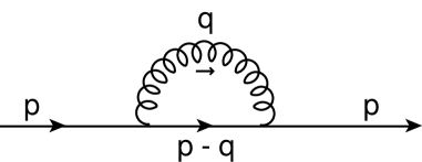
Figure 1: Quark self-energy graph. Solid lines denote quarks, curly lines gluons.

Executing the required integrations in Eq. (7), we obtain

$$\rm\Sigma^{Coul}(p)=\frac{1}{3\pi}\alpha_{s}(\not{p}-4m)\Gamma(2-\omega-\sigma)~{},$$ (10)

with $\rm\alpha_{s}\equiv\bar{g}^{2}/4\pi~{},g\equiv\bar{g}\mu^{2-\omega-\sigma}$, and $\mu$ being the mass scale. We see that the result in Eq. (10) is strictly local, despite the appearance of nonlocal integrals such as Eq. (8c).

3 Quark-quark-gluon vertex

The quark-quark-gluon vertex function $\rm\Lambda_{\mu}(p^{\prime},p)$ consists of the QED-like quark-quark-gluon vertex, $\rm\Gamma^{1}_{\mu}(p^{\prime},p)$, and the non-Abelian quark-quark-gluon vertex, $\rm\Gamma^{2}_{\mu}(p^{\prime},p)$:

$$\rm\Lambda_{\mu}(p^{\prime},p)=\Gamma^{1}_{\mu}(p^{\prime},p)+\Gamma^{2}_{\mu}(p^{\prime},p)~{}.$$ (11)

$\Gamma^{1}_{\mu}$ (Fig. 2) is the easier one to compute, containing as it does only the single noncovariant factor $\rm 1/\vec{q}^{2}$. Thus,

$$\rm\Gamma^{1}_{\mu}(p^{\prime},p)\!\! = \rm\!\!\frac{ig^{2}}{6(2\pi)^{4}}\int\frac{d^{4}q~{}\gamma_{\rho}~{}(\not{p}^{\prime}-\not{\it q}+m)\gamma_{\mu}(\not{p}-\not{\it q}+m)\gamma_{\sigma}}{q^{2}[(p^{\prime}-q)^{2}-m^{2}][(p-q)^{2}-m^{2}]}$$ (12)

$$\!\!\rm\cdot\left[g^{\rho\sigma}-\left(\frac{n^{2}{\it q}^{\rho}n^{\sigma}-q\cdot n({\it q}^{\sigma}n^{\rho}+{\it q}^{\rho}n^{\sigma})}{-\vec{\it q}^{2}}\right)\right]~{},$$

where the i$\varepsilon$-terms in the covariant propagators have been omitted for clarity. The divergent component of $\Gamma^{1}_{\mu}$ is, again, amazingly simple:

$$\rm\Gamma^{1}_{\mu}(p^{\prime},p)=\frac{\alpha_{s}}{24\pi}\gamma_{\mu}\Gamma(2-\omega-\sigma),~{}\omega\to(3/2)^{+},\sigma\to(1/2)^{+}~{}.$$ (13)

In deriving this answer, we have made use of the formulas listed in the Appendix. Notice in particular the nonlocal integrals there.

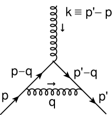
Figure 2: QED-like quark-quark-gluon vertex graph.

Computation of the non-Abelian vertex function $\rm\Gamma^{2}_{\mu}(p^{\prime},p)$ in Fig. 3,

$$\rm\Gamma^{2}_{\mu}(p^{\prime},p)\!\! = \!\!\rm\frac{i3g^{2}}{2(2\pi)^{4}}\int\frac{d^{4}q\gamma_{\sigma}(\not{p}+\not{\it q}+m)\gamma_{\nu}}{q^{2}(k-q)^{2}[(p+q)^{2}-m^{2}]}\cdot\{g^{\rho\sigma}+\frac{1}{\vec{q}^{2}}[n^{2}q^{\rho}q^{\nu}-q\cdot n(q^{\rho}n^{\nu}+q^{\nu}n^{\rho})]\}$$ (14)

$$\!\!\rm\cdot\left\{g^{\lambda\sigma}+\frac{1}{(\vec{k}-\vec{\it q})^{2}}[n^{2}(k-q)^{\lambda}(k-q)^{\sigma}-n\cdot(k-{\it q})[(k-{\it q})^{\lambda}n^{\sigma}+(k-q)^{\sigma}n^{\lambda}]]\right\}$$

$$\!\!\rm\cdot[-(k+q)_{\lambda}g_{\mu\rho}+(2q-k)_{\mu}g_{\rho\lambda}+(2k-{\it q})_{\rho}g_{\mu\lambda}]~{},k\equiv p^{\prime}-p~{},$$

is complicated by the presence of the two noncovariant factors $\rm 1/\vec{q}^{2}$ and $\rm 1/(\vec{k}-\vec{q})^{2}$, and the necessity of having to evaluate for the first time five-propagator integrals (see Section 4 for details). In fact, determination of the pole parts of these five-propagator integrals in the Coulomb gauge took as long as the rest of the calculation.

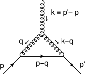
Figure 3: Non-Abelian quark-quark-gluon vertex graph.

Despite the presence of explicitly nonlocal integrals in the evaluation of $\rm\Gamma^{2}_{\mu}$, Eq. (14), the final expression turns out to be strictly local:

$$\rm\Gamma^{2}_{\mu}(p^{\prime},p)=\frac{-3\alpha_{s}}{8\pi}\gamma_{\mu}\Gamma(2-\omega-\sigma)~{},$$ (15)

so that

$$\rm\Lambda_{\mu}(p^{\prime},p)=\frac{-\alpha_{s}}{3\pi}\gamma_{\mu}\Gamma(2-\omega-\sigma)\left|{}^{\alpha\to(1/2)^{+}}_{\omega\to(3/2)^{+}}\right.~{}.$$ (16)

4 Procedure for noncovariant four-propagator and five-propagator integrals

In this section, we shall demonstrate our procedure for Coulomb-gauge integrals containing precisely two noncovariant factors of the form $\rm 1/\vec{q}^{2}$ and $\rm 1/(\vec{k}-\vec{q})^{2}$. We shall first tackle the four-propagator integral, then continue with the five-propagator case, consisting of three covariant and two noncovariant propagators.

4.1 The four-propagator integral

Application of split dimensional regularization to the Euclidean-space integral I,

$$\rm I=\int\frac{d^{2(\omega+\sigma)}{\it q}}{(2\pi)^{2(\omega+\sigma)}}\frac{1}{q^{2}(q+p)^{2}\vec{q}^{2}(\vec{q}+\vec{p})^{2}}~{},$$ (17)

yields [14]

$$\rm I\!\! = \!\!\rm\int^{1}_{0}dx\int^{x}_{0}dG\int^{1-x+G}_{G}dy\int^{\infty}_{0}dAA^{3}\int\frac{d^{2\omega}\vec{q}}{(2\pi)^{2\omega}}\int\frac{d^{2\sigma}q_{4}}{(2\pi)^{2\sigma}}$$

$$\!\!\rm\cdot exp\{-A[\vec{q}^{2}+2y\vec{q}\cdot\vec{p}+y\vec{p}^{2}+xq_{4}^{2}+2Gq_{4}p_{4}+Gp_{4}^{2}]\}~{},$$

$$= \!\!\rm\frac{\pi^{\omega+\sigma}}{(2\pi)^{2(\omega+\sigma)}}\int^{1}_{0}dx\int^{x}_{0}dG\int_{G}^{1-x+G}dy\int^{\infty}_{0}dAA^{3-\omega-\sigma}x^{-\sigma}~{}.$$

$$\!\!\rm\cdot exp\{-A[(y-y^{2})\vec{p}^{2}+G(1-G/x)p_{4}^{2}]\}~{},$$

$$= \!\!\rm\frac{\pi^{\omega+\sigma}\Gamma(4-\omega-\sigma)}{(2\pi)^{2(\omega+\sigma)}}\int^{1}_{0}dxx^{-\sigma}\int^{x}_{0}dG\int^{1-x+G}_{G}dyH^{\omega+\sigma-4}~{},$$ (19)

with

$$\rm H(x,G,y)\equiv y(1-y)\vec{p}^{2}+G(1-G/x)p_{4}^{2}~{}.$$ (20)

In order to be able to integrate over y, G and x in Eq. (19), we need to pinpoint all possible singularities in parameter space. To this effect, we observe that the integral I diverges for H = 0, i.e. for the following two cases [1]:

$$\rm Case~{}1: \!\!\rm H\to 0,~{}if~{}y=0~{}and~{}G=0~{};$$ (21a)

$$\rm Case~{}2: \!\!\rm H\to 0,~{}if~{}y=1~{}and~{}G=x~{}.$$ (21b)

Since H approaches zero linearly in Eq. (20), we may drop the terms proportional to $\rm y^{2}$ and G² in Case 1, so that

$$\rm H\to H^{(1)}_{0}=y\vec{p}^{2}+Gp_{4}^{2}~{}.$$ (22a)

Similarly, setting $\rm 1-y\equiv Y$, and $\rm x-G\equiv t$ in Case 2, we may drop the terms proportional to Y² and t², in which case

$$\rm H\to H_{0}^{(2)}=(1-y)\vec{p}^{2}+(x-G)p_{4}^{2}~{}.$$ (22b)

Accordingly, both $\rm H_{0}^{(1)}$ and $\rm H^{(2)}_{0}$ contribute to the pole part of I:

$$\rm I=\frac{\pi^{\omega+\sigma}\Gamma(2-\omega-\sigma)}{(2\pi)^{2(\omega+\sigma)}}\int^{1}_{0}dxx^{-\sigma}\int^{x}_{0}dG\int^{1-x+G}_{G}dy(H_{0}^{(1)}+H_{0}^{(2)})^{\omega+\sigma-4}+Finite~{}Terms~{},$$ (23)

or, since

$$\rm[\int dy(...)]_{{\phantom{Sum}}^{\rm y=1}_{\rm G=x}}=[\int dy(...)]_{{\phantom{Sum}}^{\rm y=0}_{\rm G=0}}~{},$$ (24)

$$\rm I=\frac{2\Gamma(4-\omega-\sigma)}{(4\pi)^{2}}\int^{1}_{0}dxx^{-\sigma}\int^{x}_{0}dG\int^{1-x+G}_{G}dy~{}[~{}H_{0}^{(1)}~{}]^{\omega+\sigma-4}+F.T.$$ (25)

Hence,

$$\rm I \rm=\displaystyle\frac{2\Gamma(4-\omega-\sigma)}{(4\pi)^{2}}\int^{1}_{0}dxx^{-\sigma}\int^{x}_{0}dGG^{\omega+\sigma-3}+F.T.~{},$$ (26)

$$\rm=\displaystyle\frac{2\Gamma(4-\omega-\sigma)}{(4\pi)^{2}p^{2}\vec{p}^{2}}\Gamma(\omega+\sigma-2)\int^{1}_{0}dxx^{\omega-2}+F.T.~{},$$ (27)

or, finally

$$\rm div\int\frac{d^{4}q}{(2\pi)^{4}}\frac{1}{q^{2}(q+p)^{2}\vec{p}^{2}(\vec{q}+\vec{p})^{2}}=\frac{-4\Gamma(2-\omega-\sigma)}{p^{2}\vec{p}^{2}(4\pi)^{2}}\left|{\begin{array}[]{l}{\scriptstyle\sigma\to(1/2)^{+}}\\ \\ {\scriptstyle\omega\to(3/2)^{+}}\\ \end{array}}~{},\right.$$ (28)

which is the result previously given in Table A.1 of Ref. [1]. Notice that the above noncovariant integral has both a three-dimensional and a four-dimensional nonlocality.

4.2 The five-propagator integral

We now turn our attention to the massive five-propagator integral I in Euclidean space,

$$\rm I=\int\frac{d^{4}q}{(2\pi)^{4}}\frac{{\it q}_{i}}{q^{2}(q-k)^{2}[(p+q)^{2}+m^{2}]\vec{q}^{2}(\vec{q}-\vec{k})^{2}}~{},k\equiv p^{\prime}-p,~{}i=1,2,3~{},$$ (29)

which is seen to possess two noncovariant and three covariant propagators. Employing a special parametrization [14], we may re-write I as

$$\rm I=\left\{\int^{1}_{0}dx\int^{x}_{0}dG\int^{1-x+G}_{G}dy\int^{x-G}_{0}dv\right\}\int^{\infty}_{0}dAA^{4}\int\frac{d^{4}q}{(2\pi)^{4}}~{}{\it q}_{i}~{}e^{-E}~{},$$ (30)

where:

$$\rm E\!\! = \!\!\rm Ax(q_{4}+r_{4})^{2}+A(\vec{q}+\vec{r})^{2}+AZ~{},$$

$$\rm r_{i}\!\! = \!\!\rm vp_{i}-yk_{i}~{},~{}~{}~{}~{}r_{4}=x^{-1}(vp_{4}-Gk_{4})~{},~{}~{}~{}~{}i=1,2,3~{},$$ (31)

$$\rm Z \!\!= \!\!\rm v[p^{2}+m^{2}+2Gp_{4}k_{4}/x-v\vec{p}^{2}+2y\vec{p}\cdot\vec{k}]+y(1-y)\vec{k}^{2}+G(x-G)k_{4}^{2}/x-v^{2}p_{4}^{2}/x~{},$$

so that

$$\rm I=\{...\}\int^{\infty}_{0}dAA^{4}e^{-AZ}\int d^{3}\vec{q}~{}{\it q}_{i}~{}e^{-A(\vec{q}+\vec{r})^{2}}\int d{\it q}_{4}~{}e^{-Ax(q_{4}+r_{4})^{2}}~{}.$$

Defining

$$\rm Q_{i}\equiv{\it q}_{i}+r_{i}~{},~{}~{}~{}~{}~{}Q_{4}\equiv{\it q}_{4}+r_{4}~{},~{}~{}~{}~{}~{}i=1,2,3~{},$$

and implementing split dimensional regularization, we find that

$$\rm I\!\! = \!\!\rm\{...\}\int^{\infty}_{0}dAA^{4}e^{-AZ}\int\frac{d^{2\omega}\vec{Q}}{(2\pi)^{2\omega}}(Q_{i}-r_{i})~{}e^{-A\vec{Q}^{2}}\int\frac{d^{2\sigma}Q_{4}}{(2\pi)^{2\sigma}}~{}e^{-AxQ_{4}^{2}}~{},$$ (32)

$$= \!\!\rm\{...\}\frac{\pi^{\omega+\sigma}}{(2\pi)^{2(\omega+\sigma)}}\int^{\infty}_{0}dAA^{4-\omega-\sigma}(-r_{i})x^{-\sigma}e^{-AZ}~{},$$

$$= \!\!\rm\frac{-\Gamma(5-\omega-\sigma)}{(4\pi)^{\omega+\sigma}}\int^{1}_{0}dxx^{-\sigma}\int^{x}_{0}dG\int^{1-x+G}_{G}dy\int^{x-G}_{0}dv(vp_{i}-yk_{i})Z^{\omega+\sigma-5}~{},$$ (33)

where we have made use of the following formulas:

$$\displaystyle\int \!\!\!\!\!\!\rm d^{2\omega}\vec{Q}~{}exp(-A\vec{Q}^{2})=\pi^{\omega}A^{-\omega}~{},A>0~{};$$

$$\displaystyle\int \!\!\!\!\!\!\rm d^{2\omega}\vec{Q}~{}Q_{i}~{}exp(-A\vec{Q}^{2})=0~{},i=1,2,3~{};$$

$$\displaystyle\int \!\!\!\!\!\!\rm d^{2\sigma}Q_{4}~{}exp(-AxQ_{4}^{2})=\pi^{\sigma}(Ax)^{-\sigma}~{};$$

$$\displaystyle\int^{\infty}_{0} \!\!\!\rm dAA^{4-\omega-\sigma}~{}exp(-AZ)=\Gamma(5-\omega-\sigma)Z^{\omega+\sigma-5}~{}.$$

We re-iterate that $\vec{\rm Q}$ is defined over 2$\omega$-dimensional complex space, and Q₄ over 2$\sigma$-dimensional complex space.

Our next task is to extract the pole part from the integral in Eq. (33), by locating the singularities of the integrand in four-dimensional parameter space. Proceeding as in Section 4.1, we see that Z in Eq. (31) vanishes for the following sets of integration parameters:

• $$\rm Z\!\! \to \!\!\rm 0,~{}if~{}v=0,~{}y=0,~{}G=0,~{}in~{}which~{}case$$

  $$\rm Z\!\! \to \!\!\rm Z^{(1)}_{0}=v(p^{2}+m^{2})+y\vec{k}^{2}+Gk_{4}^{2}~{}.$$ (35)

• $$\rm Z\!\! \to \!\!\rm 0,~{}if~{}v=0,~{}y=1,~{}G=x,~{}in~{}which~{}case$$

  $$\rm Z\!\! \to \!\!\rm Z_{0}^{(2)}=v(p^{2}+m^{2}+2p\cdot k)+(1-y)\vec{k}^{2}+(x-G)k_{4}^{2}~{}.$$ (36)

  To obtain $\rm Z^{(2)}_{0}$ in Eq. (36), it is convenient to introduce new parameters $\rm Y\equiv 1-y$, and $\rm t\equiv x-G$, so that

  $$\rm Z\to 0,~{}if~{}v=0,Y=0,t=0~{},$$ (37a)

  and

  $$\rm Z^{(2)}_{0}=v(\bar{p}^{2}+m^{2})+Y\vec{k}^{2}+tk_{4}^{2}~{},~{}\bar{p}^{2}\equiv p^{2}+2p\cdot k~{},$$ (37b)

  which is analogous to $\rm Z^{(1)}_{0}$ in Eq. (35).

Accordingly, the total expression for I in Eq. (33) reads:

$$\rm I\!\! = \!\!\rm\frac{-\Gamma(5-\omega-\sigma)}{(4\pi)^{\omega+\sigma}}\int^{1}_{0}dxx^{-\sigma}\int^{x}_{0}dG\int^{1-x+G}_{G}dy\int^{x-G}_{0}dv(vp_{i}-yk_{i})$$ (38)

$$\!\!\rm\cdot[(Z^{(1)}_{0})^{\omega+\sigma-5}+(Z_{0}^{(2)})^{\omega+\sigma-5}]~{}.$$

The divergent part of the contribution from $\rm Z^{(1)}_{0}$, at v = 0, y = 0, G = 0, can be shown to vanish.

To derive the pole contribution from $\rm Z^{(2)}_{0}$, we replace the parameters {x,G,y,v} by {x,t,Y,v}, whence

$$\rm\int^{1}_{0}dx\int^{x}_{0}dG\int^{1-x+G}_{G}dy\int^{x-G}_{0}dv=-\int^{1}_{0}dx\int^{x}_{0}dt\int^{t}_{1+t-x}dY\int^{t}_{0}dv~{},$$ (39)

and

$$\rm I\!\! = \!\!\rm\frac{\Gamma(5-\omega-\sigma)}{(4\pi)^{\omega+\sigma}}\int^{1}_{0}dxx^{-\sigma}\int^{x}_{0}dt\int^{t}_{1+t-x}dY\int^{t}_{0}dv(vp_{i}+Yk_{i}-k_{i})$$ (40)

$$\!\!\rm\cdot[v(\bar{p}^{2}+m^{2})+Y\vec{k}^{2}+tk_{4}^{2}]^{\omega+\sigma-5}~{}.$$

Since the integration proportional to $\rm(vp_{i}+Yk_{i})$ leads to a finite value, Eq. (40) reduces to the expression

$$\rm I\!\! = \!\!\rm\frac{-k_{i}\Gamma(5-\omega-\sigma)}{(4\pi)^{\omega+\sigma)}}(\bar{p}^{2}+m^{2})^{\omega+\sigma-3}\int^{1}_{0}dxx^{-\sigma}\int^{x}_{0}dt\int^{t}_{1+t-x}dY$$ (41)

$$\!\!\rm\cdot\int^{t}_{0}\frac{dv}{[v+(\bar{p}^{2}+m^{2})^{-1}(Y\vec{k}^{2}+tk_{4}^{2})]^{5-\omega-\sigma}}~{},$$

or, eventually, to

$$\rm div \!\!\rm\int\frac{d^{4}q~{}{\it q}_{i}}{(2\pi)^{4}q^{2}(q-k)^{2}[({\it q}+p)^{2}+m^{2}]\vec{q}^{2}(\vec{q}-\vec{k})^{2}}$$ (42)

$$\!\!\rm=\frac{-2k_{i}I^{*}}{k^{2}\vec{k}^{2}[(p+k)^{2}+m^{2}]}~{},\sigma\to(1/2)^{+},\omega\to(3/2)^{+}~{},$$

where $\rm I^{*}\equiv\Gamma(2-\omega-\sigma)/(4\pi)^{2}$. The above integral is seen to be nonlocal in both $\vec{\rm k}^{2}$ and k².

The method described here is applicable to all four- and five-propagator cases. Particularly challenging is the basic five-propagator integral, whose pole part consists of two distinct terms, namely

$$\rm div \!\!\rm\int\frac{d^{4}q}{(2\pi)^{4}q^{2}(q-k)^{2}[(p+k)^{2}+m^{2}]\vec{q}^{2}(\vec{q}-\vec{k})^{2}}$$ (43)

$$\!\!\rm=\frac{-2I^{*}}{k^{2}\vec{k}^{2}}\left(\frac{1}{p^{2}+m^{2}}+\frac{1}{(p+k)^{2}+m^{2}}\right)~{}.$$

5 BRST identity in the Coulomb gauge

It remains to convince ourselves that $\Sigma$(p) and $\Lambda_{\mu}$ in Eqs. (10) and (16) satisfy the appropriate one-loop BRST identity. In order to do that, however, we have to know what the ‘appropriate identity’ really is. The expression usually quoted in the literature has the structure

$$\rm(p^{\prime}-p)^{\mu}\Lambda_{\mu}(p^{\prime},p)=-\Sigma(p^{\prime})+\Sigma(p)~{},$$ (44)

and the question is: does this identity also hold in the Coulomb gauge, where ghosts are known to play a significant role? The answer to this question, surprisingly, is no.

According to Taylor, the correct BRST identity also involves ghost contributions, $\rm G_{1}(p^{\prime},p)$ and $\rm G_{2}(p^{\prime},p)$, and is given by [15, 16]

$$\rm(p^{\prime}-p)^{\mu}\Lambda_{\mu}(p^{\prime},p)+G_{1}(p^{\prime},p)+G_{2}(p^{\prime},p)=-\Sigma(p^{\prime})+\Sigma(p)~{}.$$ (45)

The corresponding ghost diagrams are depicted in Figs. 4a and 4b, with solid lines denoting quarks of mass m, curly lines gauge bosons, and with broken lines representing ghosts; $q$ is the internal momentum, as before, and p,p^′ are external momenta. It remains to compute the functions $\rm G_{1},G_{2}$.

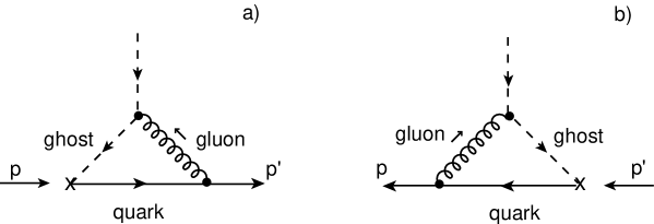
Figure 4: (a) Ghost contribution [15] to the IPI three-point function, with broken lines representing ghost particles. (b) Mirror image of the ghost diagram depicted in Fig. 4a.

The ghost diagram depicted in Fig. 4a leads in Minkowski space [15] to the expression $\rm G_{1}(p^{\prime},p)$,

$$\rm G_{1}(p^{\prime},p)\!\! = \!\!\rm[factors]~{}\int\frac{d^{4}q}{(2\pi)^{4}}\frac{1}{[(q-k)^{2}+i\varepsilon]}\left[-\delta_{ij}+\frac{(q-k)_{i}(q-k)_{j}}{(\vec{q}-\vec{k})^{2}}\right]$$ (46)

$$\!\!\rm\cdot\frac{1}{\vec{q}^{2}}{\it q}_{i}\gamma_{j}\frac{1}{(\not{p}+\not{\it q}-m+i\varepsilon)}(\not{p}-m),\varepsilon>0,k\equiv p^{\prime}-p~{}.$$

Applying the technique of split dimensional regularization to all Coulomb-gauge integrals, and utilizing the formulas in the Appendix, we find that the divergent part of G₁ is zero, i.e.

$$\rm divG_{1}(p^{\prime},p)=0~{}.$$ (47a)

A similar result may be established from Fig. 4b for G₂:

$$\rm divG_{2}(p^{\prime},p)=0~{}.$$ (47b)

In summary, neither G₁ nor G₂ contributes to the BRST identity in Eq. (45), which is obviously satisfied by $\Sigma(p)$ and $\Lambda_{\mu}(p^{\prime},p)$. After completion of this work, we discovered that an identity closely resembling the identity in Eq. (45) had been studied by Muzinich and Paige [11] and, more recently, by Newton [17] using a new approach.

6 Genuine energy integrals at two loops

The purpose of this section is to discuss briefly the application of split dimensional regularization at the two-loop level [18, 19]. In particular, we would like to know to what extent the new Coulomb-gauge technique is capable of regulating both the divergences from the notorious two-loop energy integrals [5, 6, 7, 8], as well as the ordinary UV divergences. The safest way of getting at least a partial answer to this question is to embark on an explicit two-loop calculation and then see what happens to the ambiguous energy integrals. A program of this kind has recently been initiated by the author, but the final results won’t be available for at least a year or two. In the meantime, we shall confine ourselves to a few general remarks.

Our first comment deals with the measure $\rm d^{4}q~{}d^{4}k$ of a two-loop integral. Applying rule (1) for one-dimensional integrals, we employ exactly two complex-dimensional parameters $\omega$ and $\sigma$, thus replacing the measure by

$$\rm d^{2(\omega+\sigma)}q~{}d^{2(\omega+\sigma)}k=d^{2\sigma}q_{0}~{}d^{2\omega}\vec{q}~{}d^{2\sigma}k_{0}~{}d^{2\omega}\vec{k}~{};$$ (48)

the limits $\sigma\to(1/2)^{+}$, and $\omega\to(3/2)^{+}$ are taken after all integrations have been executed.

Next, a general two-loop Coulomb-gauge integral is expected to give rise to simple and double poles, proportional to $\Gamma(2-(\omega+\sigma))$ and $[\Gamma(2-(\omega+\sigma))]^{2}$, respectively; notice that $\omega$ and $\sigma$ appear additively.

We now turn our attention to a typical energy integral, such as [7]

$$\rm I=\int\frac{dq_{0}}{2\pi}\int\frac{dk_{0}}{2\pi}\,\frac{k_{0}}{(k_{0}^{2}-\vec{k}^{2}+i\epsilon)}\,\frac{q_{0}}{(q_{0}^{2}-\vec{q}^{2}+i\epsilon)}\,,\qquad\epsilon>0,$$ (49)

which occurs for the first time at two loops. According to Doust and Taylor [6, 7, 8], standard dimensional regularization is incapable of handling the ambiguities in integrals like (49). In order to treat (49), Doust and Taylor use a special regularization, called $\theta$-regularization, which assigns to (49) a particular value, such as $1/12$. Our approach to this problem is somewhat different: by applying split dimensional regularization to a certain two-loop integral, we hope to regulate both its ordinary UV divergences, as well as the ambiguities from its energy integrals. However, before discussing a specific example, we shall briefly indicate how energy integrals such as (49) arise in practice.

Let us consider the two-loop Yang-Mills self-energy in the Coulomb gauge, specifically the sunset diagram (it possesses overlapping divergences). The amplitude for this challenging diagram reads as follows (we employ the notation of Ref. [20]):

$$\rm\Pi^{af}_{\mu\nu}(p)=\frac{1}{3!}\int\!\!\int\frac{d^{4}q~{}d^{4}k}{(2\pi)^{8}}\,V^{abcd}_{\mu\lambda\sigma\rho}\,G^{dg}_{\rho\alpha}(q)\,G^{ch}_{\sigma\beta}(p-k-q)\,G^{be}_{\lambda\xi}(k)\,V^{ghef}_{\alpha\beta\xi\nu}~{},$$ (50)

where $\rm G^{ab}_{\mu\nu}(q)$ represents the gluon propagator in the Coulomb gauge, Eq. (4), and

$$\rm V^{abcd}_{\mu\lambda\sigma\rho}\!\! = \!\!\rm-ig^{2}[f^{abe}f^{cde}(\delta_{\mu\sigma}\delta_{\lambda\rho}-\delta_{\mu\rho}\delta_{\lambda\sigma})$$ (51)

$$\quad\rm+\,f^{ace}f^{bde}(\delta_{\mu\lambda}\delta_{\sigma\rho}-\delta_{\mu\rho}\delta_{\lambda\sigma})+f^{ade}f^{cbe}(\delta_{\mu\sigma}\delta_{\lambda\rho}-\delta_{\mu\lambda}\delta_{\sigma\rho})]$$

denotes the four-gluon vertex of zero-loop order. Reduction of the integrand yields, in Euclidean space,

$$\rm\Pi^{af}_{\mu\nu}(p)\!\! = \!\rm(coeff.)\,\delta^{af}g^{4}\int\!\!\int\frac{d^{4}q~{}d^{4}k}{q^{2}k^{2}(p-k-q)^{2}}M_{\mu\sigma\lambda\rho\alpha\xi\beta\nu}$$ (52)

$$\!\!\times\ \rm[A_{\rho\alpha\lambda\xi}(q,k;n)+B_{\rho\alpha\lambda\xi}(q,k;n)]\,C_{\sigma\beta}(q,k;p,n)~{},$$

where:

$$\rm M_{\mu\sigma\lambda\rho\alpha\xi\beta\nu}\!\! = \rm 3\delta_{\mu\sigma}\delta_{\lambda\rho}\,(2\delta_{\alpha\xi}\delta_{\beta\nu}-\delta_{\alpha\nu}\delta_{\beta\xi}-\delta_{\alpha\beta}\delta_{\xi\nu})$$ (53)

$$\!\!\!\!\!+\,3\delta_{\mu\rho}\delta_{\lambda\sigma}\,(2\delta_{\alpha\nu}\delta_{\beta\xi}-\delta_{\alpha\xi}\delta_{\beta\nu}-\delta_{\alpha\beta}\delta_{\xi\nu})$$

$$\!\!\!\!\!+\,3\delta_{\mu\lambda}\delta_{\sigma\rho}\,(2\delta_{\alpha\beta}\delta_{\xi\nu}-\delta_{\alpha\xi}\delta_{\beta\nu}-\delta_{\alpha\nu}\delta_{\beta\xi})~{};$$

$$\rm A_{\rho\alpha\lambda\xi}(q,k;n)\!\! = \rm\delta_{\rho\alpha}\delta_{\lambda\xi}-\frac{k\cdot n\,\delta_{\rho\alpha}n_{\lambda}k_{\xi}}{\vec{k}^{2}}-\frac{k\cdot n\,\delta_{\rho\alpha}n_{\xi}k_{\lambda}}{\vec{k}^{2}}-\frac{q\cdot n\,\delta_{\lambda\xi}n_{\rho}q_{\alpha}}{\vec{q}^{2}}$$ (54)

$$\!\rm-~{}\frac{q\cdot n\,\delta_{\lambda\xi}n_{\alpha}q_{\rho}}{\vec{q}^{2}}+\frac{q\cdot n\,k\cdot n\,(n_{\rho}q_{\alpha}+n_{\alpha}q_{\rho})(n_{\lambda}k_{\xi}+n_{\xi}k_{\lambda})}{\vec{q}^{2}\vec{k}^{2}}~{};$$

$$\rm C_{\sigma\beta}=\delta_{\sigma\beta}+\left(\frac{n^{2}R_{\sigma}R_{\beta}-R\cdot n\,(R_{\sigma}n_{\beta}+R_{\beta}n_{\sigma})}{-\vec{R}^{2}}\right)~{},\qquad R_{\sigma}\equiv(p-k-q)_{\sigma}~{};$$ (55)

$\rm B_{\rho\alpha\lambda\xi}$ consists of four terms, but is not required for our purposes. Substitution of expressions (53)-(55) into Eq. (52) leads to three kinds of integrals: (i) covariant integrals, (ii) noncovariant Coulomb-gauge integrals, and finally, (iii) noncovariant Coulomb-gauge energy integrals. At present, we are only interested in extracting a few integrals in category (iii).

To locate a $k_{0}$ energy integral, for instance, we multiply the seventh term in $\rm M_{\mu\sigma\lambda\rho\alpha\xi\beta\nu}$ by the second term in $\rm A_{\rho\alpha\lambda\xi}$, and then contract the resulting expression with the $\rm n^{2}R_{\sigma}R_{\beta}$-term in $\rm C_{\sigma\beta}$. Thus,

$$\rm T_{\mu\nu}^{(1)}\!\! = \!\!\rm(6\delta_{\mu\lambda}\delta_{\sigma\rho}\delta_{\alpha\beta}\delta_{\xi\nu})\left[\frac{-k\cdot n\,\delta_{\rho\alpha}n_{\lambda}k_{\xi}}{\vec{k}^{2}}\right]\left(\frac{n^{2}R_{\sigma}R_{\beta}}{-\vec{R}^{2}}\right)~{},$$ (56)

$$= \!\!\rm\frac{6\,k\cdot n\,R^{2}n_{\mu}k_{\nu}}{\vec{k}^{2}\vec{R}^{2}}~{},$$

so that the corresponding integral from Eq. (52) reads

$$\rm I_{\mu\nu}^{(1)}\equiv n_{\mu}\int\frac{d^{4}q~{}d^{4}k~{}k\cdot n~{}k_{\nu}}{q^{2}k^{2}\vec{k}^{2}(\vec{p}-\vec{k}-\vec{q})^{2}}~{},$$ (57)

or, in Minkowski-space,

$$\rm I_{\mu\nu}^{(1)}=(\dots)n_{\mu}\int\frac{d^{4}q}{(q^{2}+i\epsilon)}\int\frac{d^{3}\vec{k}}{\vec{k}^{2}(\vec{p}-\vec{k}-\vec{q})^{2}}\int\frac{dk_{0}~{}k_{0}\,k_{\nu}}{(k^{2}+i\epsilon)}~{},\qquad k\cdot n=k_{0}\,,$$ (58)

leading to the $k_{0}$ energy integral

$$\rm\int\frac{dk_{0}~{}k_{0}}{(k_{0}^{2}-\vec{k}^{2}+i\epsilon)}~{}.$$ (59)

Similarly, multiplying the fourth term in $\rm M_{\mu\sigma\lambda\rho\alpha\xi\beta\nu}$ by the fourth term in $\rm A_{\rho\alpha\lambda\xi}$, and contracting with $\rm n^{2}R_{\sigma}R_{\beta}$ in $\rm C_{\sigma\beta}$, we find that

$$\rm T_{\mu\nu}^{(2)}\equiv 6\,q\cdot n\,R^{2}n_{\mu}q_{\nu}/(\vec{q}^{2}\vec{R}^{2})~{}.$$ (60)

The corresponding integral contains a $q_{0}$ energy integral of the form

$$\rm\int\frac{dq_{0}~{}q_{0}}{(q_{0}^{2}-\vec{q}^{2}+i\epsilon)}~{}.$$ (61)

To conclude this section, we shall illustrate how split dimensional regularization handles energy integrals like (49),

$$\rm I=\int\frac{dq_{0}}{2\pi}\int\frac{dk_{0}}{2\pi}\,\frac{k_{0}}{(k_{0}^{2}-\vec{k}^{2}+i\epsilon)}\,\frac{q_{0}}{(q_{0}^{2}-\vec{q}^{2}+i\epsilon)}\,,\qquad\epsilon>0,$$ (62)

which corresponds to the integral (1.3) in Doust [7]. Defining first $k_{0}$ and $q_{0}$ each over $2\sigma$-dimensional space (and labeling them $K_{\mu}$ and $Q_{\mu}$, respectively), and then defining $\rm\vec{k}$ and $\rm\vec{q}$ each over $2\omega$-dimensional space (labeling them $\vec{K}$ and $\vec{Q}$, respectively), we may rewrite (62) as

$${\rm I}_{M}=\int\frac{d^{2\sigma}Q}{(2\pi)^{2\sigma}}\int\frac{d^{2\sigma}K}{(2\pi)^{2\sigma}}\,\frac{K_{\mu}}{(K^{2}-\vec{K}^{2}+i\epsilon)}\,\frac{Q_{\mu}}{(Q^{2}-\vec{Q}^{2}+i\epsilon)}\,,\qquad\epsilon>0;$$ (63)

$K^{2}$ and $Q^{2}$ denote the squares of the $2\sigma$-dimensional vectors $K_{\mu}$ and $Q_{\mu}$, respectively, while $\vec{K}^{2}$ and $\vec{Q}^{2}$ are the squares of the $2\omega$-dimensional vectors $\vec{K}$ and $\vec{Q}$, i.e. the squares of the original 3-vectors $\rm\vec{k}$ and $\rm\vec{q}$. Wick-rotating ${\rm I}_{M}$ to Euclidean space, we obtain

$${\rm I}_{E}=\int\frac{d^{2\sigma}Q}{(2\pi)^{2\sigma}}\int\frac{d^{2\sigma}K}{(2\pi)^{2\sigma}}\,\frac{K_{\mu}}{(K^{2}+\vec{K}^{2})}\,\frac{Q_{\mu}}{(Q^{2}+\vec{Q}^{2})}~{}.$$ (64)

Since each one of the integrals in (64) is now well defined, we may apply standard dimensional regularization to get

$$\int\frac{d^{2\sigma}Q}{(2\pi)^{2\sigma}}\frac{Q_{\mu}}{(Q^{2}+\vec{Q}^{2})}\ =0\,,\qquad\int\frac{d^{2\sigma}K}{(2\pi)^{2\sigma}}\frac{K_{\mu}}{(K^{2}+\vec{K}^{2})}\ =0\,,$$ (65)

so that $\rm I=0$. Consequently, in split dimensional regularization, the ambiguous energy integral (62), or (49), has the value zero.

7 Conclusion

In this paper we have carried out a second test of split dimensional regularization by evaluating to one loop the pole parts of the quark self-energy $\rm\Sigma(p)$, and the quark-quark-gluon vertex $\rm\Lambda_{\mu}(p^{\prime},p)$. The technique of split dimensional regularization was specifically designed to regulate Feynman integrals in the noncovariant Coulomb gauge $\rm\vec{\bigtriangledown}\cdot\vec{A}^{a}(x)=0$. Its most important single feature is the use of two complex parameters, $\omega$ and $\sigma$, which permit us to regulate the divergences of certain energy-integrals.

The results in this paper may be summarized as follows.

1. Split dimensional regularization enables us to compute unambiguously all relevant one-loop integrals in the Coulomb gauge. This comment applies especially to the noncovariant four- and five-propagator integrals appearing in the vertex function $\rm\Lambda_{\mu}(p^{\prime},p)$ (Section 4).

2. The conventional BRST identity in Eq. (44) should by rights be replaced by the general BRST identity in Eq. (45). The latter contains two new functions, G₁ and G₂, which correspond to the ghost vertex diagrams shown in Figs. 4a and 4b, respectively. An explicit calculation of $\rm G_{1}(p^{\prime},p)$ and $\rm G_{2}(p^{\prime},p)$ reveals, however, that the pole parts of these functions are actually zero.

3. Computation of $\rm\Gamma^{1}_{\mu}(p^{\prime},p)$ and $\rm\Gamma^{2}_{\mu}(p^{\prime},p)$ involves several complicated Coulomb-gauge integrals, some of which turn out to be nonlocal. Nevertheless, both $\Gamma_{\mu}^{1}$ and $\Gamma^{2}_{\mu}$ are strictly local and respect, together with $\Sigma$(p), the correct BRST identity in Eq. (45).

4. Although ghosts generally play an important role in the Coulomb gauge, they do not contribute explicitly to the BRST identity relating $\Lambda_{\mu}$ and $\Sigma$(p).

Appendix

The following Coulomb-gauge Feynman integrals, defined over 2($\omega+\sigma$)-dimensional complex Euclidean space, are useful in the evaluation of $\Sigma$(p), $\Gamma^{1}_{\mu}$ and $\Gamma^{2}_{\mu}$ in Eqs. (10), (13) and (15), respectively. We employ the abbreviations

$$\rm dq\equiv d^{3}\vec{q}dq_{4}/(2\pi)^{4}~{},$$

and

$$\rm I^{*}\equiv\frac{\Gamma(2-\omega-\sigma)}{(4\pi)^{2}}\left|{\begin{array}[]{l}{\scriptstyle\sigma\to(1/2)^{+}}\\ \\ {\scriptstyle\omega\to(3/2)^{+}}\\ \end{array}}~{}.\right.$$

$$\rm div \!\!\rm\int\frac{dq~{}{\it q}_{i}{\it q}_{j}q_{4}}{q^{2}[(q+p)^{2}+m^{2}]\vec{q}^{2}}=-\frac{1}{6}p_{4}\delta_{ij}I^{*}~{},$$

$$\rm div \!\!\rm\int\frac{dq~{}q_{4}^{3}}{q^{2}[(q+p)^{2}+m^{2}]\vec{q}^{2}}=-\frac{3}{2}p_{4}I^{*}~{},$$

$$\rm div \!\!\rm\int\frac{dq~{}{\it q}_{i}{\it q}_{j}q_{4}^{2}}{(q+p)^{2}\vec{q}^{2}(\vec{q}+\vec{p})^{2}}=\delta_{ij}\left(\frac{2}{15}\vec{p}^{2}+\frac{2}{3}p_{4}^{2}\right)I^{*}-2p_{i}p_{j}\left(\frac{1}{5}+p_{4}^{2}/(\vec{p}^{2})\right)I^{*}~{},$$

$$\rm div \!\!\rm\int\frac{dq}{(p^{\prime}+q)^{2}[(q+p)^{2}+m^{2}]\vec{q}^{2}}=0~{},$$

$$\rm div \!\!\rm\int\frac{dq~{}{\it q}_{i}q_{4}}{(p^{\prime}+q)^{2}[(p+q)^{2}+m^{2}]\vec{q}^{2}}=0~{},i=1,2,3~{},$$

$$\rm div \!\!\rm\int\frac{dq}{[(p^{\prime}+q)^{2}+m^{2}][(p+q)^{2}+m^{2}]\vec{q}^{2}}=0~{},$$

$$\rm div \!\!\rm\int\frac{dq~{}{\it q}_{i}{\it q}_{j}}{[(p^{\prime}+q)^{2}+m^{2}][(p+q)^{2}+m^{2}]\vec{q}^{2}}=\frac{1}{3}\delta_{ij}I^{*}~{},$$

$$\rm div \!\!\rm\int\frac{dq}{q^{2}(p^{\prime}+q)^{2}[(p+q)^{2}+m^{2}]\vec{q}^{2}}=\frac{-2I^{*}}{(p^{\prime})^{2}(p^{2}+m^{2})}~{},$$

$$\rm div \!\!\rm\int\frac{dq~{}{\it q}_{i}{\it q}_{j}}{q^{2}(p^{\prime}+q)^{2}[(p+q)^{2}+m^{2}]\vec{q}^{2}}=0~{},$$

$$\rm div \!\!\rm\int\frac{dq~{}{\it q}_{i}{\it q}_{j}}{q^{2}[(p^{\prime}+q)^{2}+m^{2}][(p+q)^{2}+m^{2}]\vec{q}^{2}}=0~{},$$

$$\rm div \!\!\rm\int\frac{dq}{q^{2}[(p+q)^{2}+m^{2}](\vec{q}+\vec{p}^{\prime})^{2}\vec{q}^{2}}=\frac{-2I^{*}}{(\vec{p}^{\prime})^{2}(p^{2}+m^{2})}~{},$$

$$\rm div \!\!\rm\int\frac{dq~{}{\it q}_{i}}{q^{2}[(p+q)^{2}+m^{2}](\vec{q}+\vec{p}^{\prime})^{2}\vec{q}^{2}}=0~{},$$

$$\rm div \!\!\rm\int\frac{dq~{}{\it q}_{i}q_{4}}{q^{2}[(p+q)^{2}+m^{2}](\vec{q}+\vec{p}^{\prime})^{2}\vec{q}^{2}}=0~{},$$

$$\rm div \!\!\rm\int\frac{dq~{}{\it q}_{i}q_{j}}{q^{2}(p^{\prime}+q)^{2}[(p+q)^{2}+m^{2}](\vec{q}+\vec{p}^{\prime})^{2}\vec{q}^{2}}=\frac{-2p^{\prime}_{i}p^{\prime}_{j}I^{*}}{(p^{\prime})^{2}(\vec{p}^{\prime})^{2}[(p-p^{\prime})^{2}+m^{2}]}~{}.$$

References

• [1] G. Leibbrandt and J. Williams, Nucl. Phys. B475 (1996) 469.
• [2] G. Leibbrandt, Noncovariant Gauges, World Scientific Publishing Co., 1994.
• [3] J. Schwinger, Phys. Rev. 127 (1962) 324.
• [4] N.H. Christ and T.D. Lee, Phys. Rev. D22 (1980) 939.
• [5] H. Cheng and Er-Cheng Tsai, Phys. Rev. D36 (1987) 3196.
• [6] J.C. Taylor, in Physical and Non-standard Gauges, eds. P. Gaigg, W. Kummer and M. Schweda, Lecture Notes in Physics, Vol. 361 (Springer, Berlin, 1990) p. 137.
• [7] P.J. Doust, Ann. Phys. (NY) 177 (1987) 169.
• [8] P.J. Doust and J.C. Taylor, Phys. Lett. B197 (1987) 232.
• [9] G. Leibbrandt, in MRST ’96. Proc. Eighteenth Annual Montréal–Rochester–Syracuse
Toronto Meeting, 9–10 May, 1996; Toronto, Canada (World Scientific, Singapore) pp. 1–7.
• [10] G. Leibbrandt, Split dimensional regularization in the Coulomb gauge. XXVIII International Conference on High Energy Physics, Warsaw, Poland, July 25–31, 1996 (World Scientific, Singapore, 1997), Vol. II, pp. 1639–1641.
• [11] I.J. Muzinich and F.E. Paige, Phys. Rev. D21 (1980) 1151.
• [12] J. Frenkel and J.C. Taylor, Nucl. Phys. B109 (1976) 439.
• [13] R.N. Mohapatra, Phys. Rev. D4 (1971) 378.
• [14] The author is indebted to his student, J. Williams, for providing him with this particularly convenient parametrization.
• [15] The author is grateful to Professor J.C. Taylor for alerting him about the existence [16] of the ghost contributions $\rm G_{1}(p^{\prime},p)$ and $\rm G_{2}(p^{\prime},p)$ in Eq. (45), and for explaining to him their graphical representation in terms of ‘ordinary’ Feynman diagrams.
• [16] J.C. Taylor, Nucl. Phys. B33 (1971) 436.
• [17] C. Newton, private communication (1997).
• [18] W. Lucha, F.F. Schöberl, D. Gromes, Phys. Rep. 200 (1991) 127.
• [19] W. Kummer and W. Mödritsch, Z. Phys. C66 (1995) 225; W. Kummer, W. Mödritsch and A. Vairo, Z. Phys. C72 (1996) 653.
• [20] G. Leibbrandt and S.-L. Nyeo, J. Math. Phys. 27 (1986) 627.