Type IIB Orientifolds, F-theory, Type I Strings on Orbifolds
and Type I - Heterotic Duality

Abstract

We consider six and four dimensional ${\cal N}=1$ supersymmetric orientifolds of Type IIB compactified on orbifolds. We give the conditions under which the perturbative world-sheet orientifold approach is adequate, and list the four dimensional ${\cal N}=1$ orientifolds (which are rather constrained) that satisfy these conditions. We argue that in most cases orientifolds contain non-perturbative sectors that are missing in the world-sheet approach. These non-perturbative sectors can be thought of as arising from D-branes wrapping various collapsed 2-cycles in the orbifold. Using these observations, we explain certain “puzzles” in the literature on four dimensional orientifolds. In particular, in some four dimensional orientifolds the “naive” tadpole cancellation conditions have no solution. However, these tadpole cancellation conditions are derived using the world-sheet approach which we argue to be inadequate in these cases due to appearance of additional non-perturbative sectors. The main tools in our analyses are the map between F-theory and orientifold vacua and Type I-heterotic duality. Utilizing the consistency conditions we have found in this paper, we discuss consistent four dimensional chiral ${\cal N}=1$ Type I vacua which are non-perturbative from the heterotic viewpoint.

I Introduction

In ten dimensions there are five consistent string theories. The first four, Type IIA, Type IIB, $E_{8}\otimes E_{8}$ heterotic and ${\mbox{Spin}}(32)/{\bf Z}_{2}$ heterotic, are theories of oriented closed strings. The last one, Type I, is a theory of both unoriented closed and open strings. Perturbatively, these five theories are apparently different. In recent years, however, a unified picture has emerged, where the five string theories appear as different regimes of an underlying theory related via a web of conjectured dualities in ten and lower dimensions. Most of these dualities are intrinsically non-perturbative, and often shed light on non-perturbative phenomena in one theory by mapping them to perturbative phenomena in another theory.

As to the perturbative formulation, the four oriented closed string theories are relatively well understood. Conformal field theory and modular invariance serve as guiding principles for perturbative model building in closed string theories. Type I, however, still remains the least understood string theory even perturbatively. This is in part due to lack of modular invariance, which is necessary for perturbative consistency of oriented closed string theories.

In the past years various unoriented closed plus open string vacua have been constructed using orientifold techniques. Type IIB orientifolds are generalized orbifolds that involve world-sheet parity reversal along with geometric symmetries of the theory. The orientifold procedure results in an unoriented closed string theory. Consistency then generically requires introducing open strings that can be viewed as starting and ending on D-branes [1]. In particular, Type I compactifications on toroidal orbifolds can be viewed as Type IIB orientifolds with a certain choice of the orientifold projection. Global Chan-Paton charges associated with D-branes manifest themselves as a gauge symmetry in space-time. D-branes (as well as orientifold planes) are coherent states [2, 3] built from a superposition of an infinite tower of closed string oscillators acting on the momentum and/or winding states.

To ensure that a given orientifold model gives rise to a consistent string theory it is necessary to make sure that the underlying conformal field theory satisfies certain self-consistency requirements. However, conformal field theories on world-sheets with boundaries (ultimately present in an open sting theory) are still poorly understood. To circumvent these difficulties some techniques have been developed in the past (see, e.g., [2, 3, 4, 5, 6]). The idea is to implement factorization of loop amplitudes (to ensure, say, consistency of closed-to-open string transitions), generalized GSO projections (to guarantee correct spin-statistics relation in space-time), and (at the last step) tadpole cancellation (which is required for finiteness). In this approach space-time anomaly cancellation is expected to be guaranteed by the world-sheet consistency of the theory, just as in oriented closed string theories.

These techniques have been (rather) successfully applied to the construction of six dimensional ${\cal N}=1$ space-time supersymmetric orientifolds of Type IIB compactified on orbifold limits of K3 (that is, toroidal orbifolds $T^{4}/{\bf Z}_{N}$, $N=2,3,4,6$). In particular, the ${\bf Z}_{2}$ orbifold case [7, 8] has been studied in detail. This construction was subsequently generalized to other orbifold limits of K3 (namely, ${\bf Z}_{N}$ with $N=3,4,6$) in Refs [9, 10]. These orientifold models contain more than one tensor multiplet in their massless spectra, and, therefore, describe six dimensional vacua which are non-perturbative from the heterotic viewpoint.

It is natural to expect that these orientifold constructions should be generalizable to the cases of four dimensional ${\cal N}=1$ space-time supersymmetric orientifolds of Type IIB on orbifold limits of Calabi-Yau three-folds (that is, toroidal orbifolds $T^{4}/G$ with $SU(3)$ holonomy). Understanding such compactifications is extremely desirable as according to the conjectured Type I-heterotic duality [11] certain non-perturbative heterotic phenomena are expected to have perturbative Type I origins. In particular, non-perturbative dynamics of heterotic NS 5-branes under this duality is mapped to (at least naively) perturbative dynamics of Type I D5-branes.

The first example of a four dimensional ${\cal N}=1$ Type I vacuum was constructed in Ref [12] as an orientifold of Type IIB on a ${\bf Z}_{2}\otimes{\bf Z}_{2}$ toroidal orbifold. This model has enhanced gauge symmetries from D5-branes which are non-perturbative from the heterotic viewpoint. This vacuum is non-chiral, however. To obtain chiral vacua it is natural to try other orbifold groups. The first example of a chiral ${\cal N}=1$ Type I vacuum in four dimensions was constructed in Ref [13] via an orientifold of Type IIB on the $Z$-orbifold. This vacuum contains no D5-branes, and it was shown to be dual to a perturbative heterotic vacuum in Ref [14]. (Other examples of such Type I vacua have been constructed in Refs [15, 16] via orientifolds of Type IIB on ${\bf Z}_{7}$ and ${\bf Z}_{3}\otimes{\bf Z}_{3}$ orbifolds.)

Subsequently, the first four dimensional chiral ${\cal N}=1$ Type I vacuum which is non-perturbative from the heterotic viewpoint was constructed in Ref [16] via an orientifold of Type IIB on a ${\bf Z}_{6}$ orbifold. This model has D5-branes giving rise to enhanced gauge symmetries which are non-perturbative from the heterotic viewpoint.

In Ref [17] an attempt was made to extend the work in Refs [12, 13, 15, 16] to the four dimensional ${\bf Z}_{N}\otimes{\bf Z}_{M}$ orbifold cases. However, a bothersome puzzle was encountered: in some of the models the tadpole cancellation conditions (derived using the perturbative orientifold approach, namely, via a straightforward generalization of the six dimensional tadpole cancellation conditions of Refs [7, 8, 9, 10]) allowed for no solutions. This, at least at the first sight, seems surprising as Type IIB compactifications on those orbifolds are well defined, and so should be the corresponding orientifolds. This clearly indicates that a better understanding of the orientifold construction is desirable. This is precisely the subject to which this paper is devoted.

We consider six and four dimensional ${\cal N}=1$ supersymmetric orientifolds of Type IIB compactified on orbifold limits of K3 and Calabi-Yau three-folds, respectively. We study conditions necessary for world-sheet consistency of Type IIB orientifolds, that is, the conditions under which perturbative orientifold approach is adequate. We argue that in most cases orientifolds contain sectors which are non-perturbative (i.e., these sectors have no world-sheet description). These sectors can be thought of as arising from D-branes wrapping various collapsed 2-cycles in the orbifold. In particular, we argue that such non-perturbative states are present in the “anomalous” models of Ref [17] (as well as in other examples of this type recently discussed in Ref [18]). This resolves the corresponding “puzzles”. Moreover, we point out certain world-sheet consistency conditions in four dimensional cases (which are automatically satisfied in the six dimensional cases studied in Refs [7, 8, 9, 10] so their relevance cannot be appreciated in those constructions) which indicate that the only four dimensional orientifolds that have perturbative description are those of Type IIB compactified on the ${\bf Z}_{2}\otimes{\bf Z}_{2}$ [12], ${\bf Z}_{3}$ [13], ${\bf Z}_{7}$ [15], ${\bf Z}_{3}\otimes{\bf Z}_{3}$ and ${\bf Z}_{6}$ [16], and ${\bf Z}_{2}\otimes{\bf Z}_{2}\otimes{\bf Z}_{3}$ [19] orbifolds. In particular, none of the other models considered in Refs [17, 18] have perturbative orientifold description, and even in the models with all tadpoles cancelled the massless spectra given in Refs [17, 18] miss certain non-perturbative states.

The main tool in our analyses is the interplay between different string theories via the web of dualities. The relations between Type IIB orientifolds, Type I, heterotic and F-theory are schematically depicted in Fig.1. Our goal in this paper is to understand Type I compactifications and Type IIB orientifolds, and, in particular, the relation between them (which is link “b” in Fig. 1). In most cases, none of the above descriptions are completely perturbative. Nonetheless, by combining various approaches together, we are able to get much of the qualitative as well as some quantitative properties of Type I compactifications and Type IIB orientifolds. On the other hand, by studying orientifolds in various dimensions, one can obtain non-trivial information about F-theory and non-perturbative heterotic string vacua. In the following we summarize some of the important points in this approach.
$\bullet$ Type I-heterotic duality [11] (which is link “c” in Fig. 1) is crucial in checking the consistency of the models that do have perturbative heterotic duals. (To be precise, these are orientifolds which only contain D9-branes but no D5-branes. The ${\bf Z}_{3}$ [13], ${\bf Z}_{7}$ [15] and ${\bf Z}_{3}\otimes{\bf Z}_{3}$ [16] cases are examples of such orientifolds.) These checks are largely based on the observations of Ref [14] (as well as Refs [15, 16]). Moreover, we are able to determine the non-perturbative states that appear in the orientifold approach by studying the perturbative spectrum of the heterotic dual. This will be discussed in section IX.
$\bullet$ Having established the map between some orientifolds and their perturbative heterotic duals, one can use orientifold construction (with both D9- and D5-branes) as a tool to understand non-perturbative heterotic string vacua. This will be discussed in section X.
$\bullet$ The map [20] between F-theory [21] and orientifolds (which is link “a” in Fig. 1) is an invaluable tool for understanding the qualitative features of the non-perturbative states in Type IIB orientifolds (even in cases where perturbative heterotic duals do not exist). In particular, one can identify the non-perturbative states in the orientifold approach as arising from D-branes wrapping various collapsed two cycles in the orbifold. This will be discussed in section V and section VIII.
$\bullet$ By studying various orientifolds in six (and four) dimensions, one can obtain certain non-trivial information about Calabi-Yau three-fold (and four-fold) geometry along the lines of Refs [22, 23]. In section VIII, we will show that the six-dimensional ${\bf Z}_{N}$ orientifolds ($N=2,3,4,6$) [7, 8, 9, 10] are equivalent to F-theory compactifications on certain elliptically fibered Calabi-Yau three-folds, which can be regarded as extended Voisin-Borcea orbifolds [24, 25] (see Fig.2). Similarly, the four-dimensional ${\bf Z}_{2}\otimes{\bf Z}_{2}$ orientifold [12] is dual to F-theory compactification on a Borcea four-fold [25].
$\bullet$ Finally, the duality between F-theory and heterotic vacua (which is link “d” in Fig. 1) turns out to be useful in understanding certain aspects of Type I compactifications on K3. This will be discussed in details in section VIII.

The remainder of this paper is organized as follows. In section II we review some facts in conformal field theory of orbifolds and set up our notations. In section III we derive world-sheet consistency conditions for orientifolds of Type IIB on non-geometric conformal field theory orbifolds. In section IV we classify six and four dimensional orientifolds that satisfy this constraint. In section V we give F-theory interpretation of the consistency condition derived in section III. In section VI we extend these analyses to orientifolds of Type IIB on geometric conformal field theory orbifolds. In section VII we discuss six dimensional orientifolds of Refs [9, 10] and their possible generalizations to four dimensions. In particular, we point out that there are two distinct choices for the orientifold projection in six dimensions, whereas in four dimensions there is only one such choice. This is basically the reason why there are subtleties in attempting to generalize the tadpole cancellation conditions of Refs [9, 10] to four dimensions. In section VIII we give various F-theory checks for our arguments in section VII. We also discuss F-theory duals of six and four dimensional orientifolds. In section IX we review the four dimensional Type I-heterotic duality map studied in Ref [14]. In section X we demonstrate how to use this map to construct consistent four dimensional chiral ${\cal N}=1$ Type I vacua which are non-perturbative from the heterotic viewpoint. In section XI we explain the “puzzles” encountered in the literature (in particular, in Refs [17, 18]) on four dimensional orientifolds and point out which of these have perturbative description. In section XII we summarize the main conclusions of this paper. We also point out some directions for future research. Some of the details are relegated to appendices. As an aside, in appendix D we construct F-theory duals of six dimensional CHL compactifications. Although various sections are interrelated, most of them are rather self-contained and can be read separately.

II Preliminaries

In this section we review some well-known facts in conformal field theory of orbifolds. This will serve the purpose of setting up our notations and conventions, as well as emphasizing certain points which will be important in the subsequent sections.

Consider a free closed string propagating in space-time. Its world-sheet is a cylinder parametrized by a time-like coordinate $\sigma^{0}$ and a space-like coordinate $\sigma^{1}$. Let the circumference of the string be $2\pi$. Then we have the identification $\sigma^{1}=\sigma^{1}+2\pi$. Due to this identification one must specify periodicity conditions under $\sigma^{1}\rightarrow\sigma^{1}+2\pi$ for all the fields on the world-sheet.

Instead of working with $\sigma^{0}$ and $\sigma^{1}$, it is convenient to introduce the holomorphic and anti-holomorphic coordinates $z\equiv\exp(i(\sigma^{0}+\sigma^{1}))$ and ${\overline{z}}\equiv\exp(i(\sigma^{0}-\sigma^{1}))$, respectively. Then the left- and right-moving fields on the world-sheet depend only on $z$ and ${\overline{z}}$, respectively.

A Twist Fields

Let $\phi_{v}(z)$ be a single free left-moving complex world-sheet boson with the monodromy

$$\partial\phi_{v}(z{\mbox{e}}^{2\pi i})=\exp(-2\pi iv)\partial\phi_{v}(z)~{},$$ (1)

where $0<v<1$. This monodromy implies that a twist field $\sigma_{v}(z)$ is located at the origin such that

$$i\partial\phi_{v}(z)\sigma_{v}(0)\sim z^{-v}\tau_{v}(0)+\cdots~{},$$ (2)

$$i\partial\phi_{v}^{\dagger}(z)\sigma_{v}(0)\sim z^{v-1}\tau_{v}^{\prime}(0)+\cdots~{},$$ (3)

where $\phi_{v}^{\dagger}$ is the Hermitean conjugate of $\phi_{v}$, and $\tau_{v},\tau_{v}^{\prime}$ are the excited twist fields. The basic twist fields $\sigma_{v}$ has conformal dimension $v(1-v)/2$.

Next, consider a single free right-moving complex world-sheet boson ${\overline{\phi}}_{u}({\overline{z}})$ with the monodromy

$${\overline{\partial}}{\overline{\phi}}_{u}({\overline{z}}{\mbox{e}}^{-2\pi i})=\exp(+2\pi iu){\overline{\partial}}{\overline{\phi}}_{u}({\overline{z}})~{},$$ (4)

where $0<u<1$. This monodromy implies that a twist field ${\overline{\sigma}}_{u}({\overline{z}})$ is located at the origin such that

$$i{\overline{\partial}}{\overline{\phi}}_{u}({\overline{z}}){\overline{\sigma}}_{u}(0)\sim{\overline{z}}^{-u}{\overline{\tau}}_{u}(0)+\cdots~{},$$ (5)

$$i{\overline{\partial}}{\overline{\phi}}^{\dagger}_{u}({\overline{z}}){\overline{\sigma}}_{u}(0)\sim{\overline{z}}^{u-1}{\overline{\tau}}^{\prime}_{u}(0)+\cdots~{},$$ (6)

where ${\overline{\phi}}_{u}^{\dagger}$ is the Hermitean conjugate of ${\overline{\phi}}_{u}$, and ${\overline{\tau}}_{u},{\overline{\tau}}_{u}^{\prime}$ are the excited twist fields. The basic twist fields ${\overline{\sigma}}_{u}$ has conformal dimension $u(1-u)/2$.

The twist fields $\sigma_{v}$ and ${\overline{\sigma}}_{v}$ are identical. (By this we mean that $\sigma_{v}(x)={\overline{\sigma}}_{v}(x)$, where $x$ is an arbitrary complex number.) The twist fields $\sigma_{v}$ and ${\overline{\sigma}}_{1-v}$, on the other hand, are different except for $v=1/2$.

There are two inequivalent ways of combining the above left- and right-moving fields into a world-sheet boson.
$\bullet$ (i) Let $\phi_{v}(\sigma^{0},\sigma^{1})=\phi_{v}(z)+{\overline{\phi}}_{v}^{\dagger}({\overline{z}})$. This field has the following periodicity condition: $\phi_{v}(\sigma^{0},\sigma^{1}+2\pi)=\exp(-2\pi iv)\phi_{v}(\sigma^{0},\sigma^{1})$. The twisted ground state is given by $\sigma_{v}|0\rangle_{L}\otimes{\overline{\sigma}}_{v}|0\rangle_{R}$, where $|0\rangle_{L}$ and $|0\rangle_{R}$ are the left- and right-moving conformal ground states, respectively. Note that the twisted ground state in this case is left-right symmetric.
$\bullet$ (ii) Let ${\widetilde{\phi}}_{v}(\sigma^{0},\sigma^{1})=\phi_{v}(z)+{\overline{\phi}}_{1-v}({\overline{z}})$. This field has the same periodicity condition as the field $\phi_{v}(\sigma^{0},\sigma^{1})$: $\phi_{v}(\sigma^{0},\sigma^{1}+2\pi)=\exp(-2\pi iv)\phi_{v}(\sigma^{0},\sigma^{1})$. However, the twisted ground state is now given by $\sigma_{v}|0\rangle_{L}\otimes{\overline{\sigma}}_{1-v}|0\rangle_{R}$. Note that the twisted ground state in this case is left-right asymmetric unless $v=1/2$.

Here we note that in case (i) the complexification for the left- and right-movers is opposite. That is, $\phi_{v}(z)=\phi^{1}(z)+i\phi^{2}(z)$, while ${\overline{\phi}}_{v}({\overline{z}})={\overline{\phi}}^{1}({\overline{z}})-i{\overline{\phi}}^{2}({\overline{z}})$, where $\phi^{1}(z),\phi^{2}(z)$ are left-moving real world-sheet bosons, and ${\overline{\phi}}^{1}({\overline{z}}),{\overline{\phi}}^{2}({\overline{z}})$ are their right-moving counterparts. On the other hand, in case (ii) the complexification for the left- and right-movers is the same: $\phi_{v}(z)=\phi^{1}(z)+i\phi^{2}(z)$, while ${\overline{\phi}}_{1-v}({\overline{z}})={\overline{\phi}}^{1}({\overline{z}})+i{\overline{\phi}}^{2}({\overline{z}})$.

B “Symmetric” vs. “Asymmetric” Orbifolds

So far we have considered a single complex world-sheet boson. Now let us discuss toroidal orbifolds which lead to Calabi-Yau $d$-folds ($d=2,3$). First consider the following orbifold: ${\cal M}_{d}=T^{2d}/G$, where $G=\{g_{a}|a=1,\dots,{\mbox{dim}}(G)\}$ is the orbifold group. Let the twisted ground states in all of the $g_{a}$ twisted sectors be left-right symmetric as in case (i) above. We will refer to such orbifolds as “symmetric” orbifolds. Next, let us consider the following orbifold: ${\widetilde{\cal M}}_{d}=T^{2d}/{\widetilde{G}}$, where ${\widetilde{G}}=\{{\widetilde{g}}_{a}|a=1,\dots,{\mbox{dim}}({\widetilde{G}})\}$ is the orbifold group. Let the twisted ground states in all of the ${\widetilde{g}}_{a}$ twisted sectors be left-right asymmetric as in case (ii) above. (The ${\bf Z}_{2}$ twisted sectors, however, are automatically left-right symmetric.) We will refer to such orbifolds as “asymmetric” orbifolds.

Throughout this paper we will assume that ${\cal M}_{d}$ (${\widetilde{\cal M}}_{d}$) are orbifold “limits” of Calabi-Yau $d$-folds with $SU(d)$ holonomy. Let $z_{s}$, $s=1,\dots,d$, be complex coordinates parametrizing $T^{2d}$. The Calabi-Yau condition implies that $G$ (${\widetilde{G}}$) must preserve the holomorphic $d$-form $dz_{1}\wedge\dots\wedge dz_{d}$ on ${\cal M}_{d}$ (${\widetilde{\cal M}}_{d}$), so that $g_{a}$ (${\widetilde{g}}_{a}$) must act as $d\times d$ matrices on $dz_{s}$ such that $\det(g_{a})=1$ ($\det({\widetilde{g}}_{a})=1$).

Here we note that the “asymmetric” orbifolds ${\widetilde{\cal M}}_{d}$ are the “geometric” orbifolds. That is, they correspond to conformal field theory realizations of geometric quotients of the form $T^{2d}/{\widetilde{G}}$. On the other hand, the “symmetric” orbifolds ${\cal M}_{d}$ do not have an analogous geometric interpretation. They are conformal field theory constructions, and when referred to as ${\cal M}_{d}=T^{2d}/G$ orbifolds they should not be literally understood as geometric quotients. Rather, one has to bear in mind the action of the twists $g_{a}$ on left- and right-moving components of the conformal fields $z_{s}$.

The relation between the “symmetric” ${\cal M}_{d}$ and “asymmetric” ${\widetilde{\cal M}}_{d}$ orbifolds is that they are “mirror pairs”. Thus, for $d=2$ they give rise to K3 surfaces (for $G\approx{\widetilde{G}}\approx{\bf Z}_{N}$, $N=2,3,4,6$) ${\cal M}_{2}$ and ${\widetilde{\cal M}}_{2}$ which are related by a mirror transform of K3. For $d=3$ they give rise to mirror Calabi-Yau three-folds with the Hodge numbers interchanged: $(h^{1,1},h^{2,1})=({\widetilde{h}}^{2,1},{\widetilde{h}}^{1,1})$. As an example consider the $Z$-orbifold generated by the following twist: $gz_{s}=\omega z_{s}$ ($s=1,2,3$), where $\omega=\exp(2\pi i/3)$. The “asymmetric” $Z$-orbifold has the Hodge numbers $({\widetilde{h}}^{1,1},{\widetilde{h}}^{2,1})=(36,0)$, which are the same as for the familiar geometric $Z$-orbifold. The “symmetric” $Z$-orbifold has the Hodge numbers $(h^{1,1},h^{2,1})=(0,36)$, which are those of the manifold mirror to the geometric $Z$-orbifold.

Here we should point out that the terminology “symmetric” and “asymmetric” orbifolds, which we are using here, is non-standard. In particular, the standard orbifolds in Refs [26] are the geometric, that is, “asymmetric” orbifolds in our terminology. We will always use quotation marks when referring to “symmetric” and “asymmetric” orbifolds (as well as “symmetric” and “asymmetric” orientifolds - see below) as a reminder to avoid confusion.

C Torus

For our purposes in the subsequent sections it will suffice to examine the untwisted sector contributions of the bosonic world-sheet degrees of freedom $z_{s}$ into the closed string one-loop vacuum amplitude.

First, consider the one-loop vacuum amplitude for Type IIB compactified on ${\cal M}_{d}$. The closed string world-sheet is a compact Riemann surface of genus one, i.e., a two-torus. The complex structure of this two-torus is described by one complex parameter $\tau=\tau_{1}+i\tau_{2}$. (The one-loop vacuum amplitude is independent of the Kähler structure of this two-torus as a consequence of conformal invariance.) The untwisted sector contributions of the bosonic world-sheet degrees of freedom $z_{s}$ into the torus amplitude are given by (here we drop all the fermionic world-sheet degrees of freedom as well as the bosonic world-sheet degrees of freedom corresponding to non-compact coordinates, and the light-cone gauge is adapted throughout):

$${\cal T}={1\over{\mbox{dim}}(G)}\sum_{a=1}^{{\mbox{{dim}}}(G)}{\cal T}_{a}={1\over{\mbox{dim}}(G)}\sum_{a=1}^{{\mbox{{dim}}}(G)}{\mbox{Tr}}\left(g_{a}q^{L_{0}}{\overline{q}}^{{\overline{L}}_{0}}\right)~{}.$$ (7)

Here $q\equiv\exp(2\pi i\tau)$; $L_{0}$ and ${\overline{L}}_{0}$ are the left- and right-moving Hamiltonians, respectively; the trace is over the untwisted sector states corresponding to $z_{s}$ (oscillator excitations as well as momenta and windings).

Here we are considering left-right symmetric orbifolds ${\cal M}_{d}$. Then the operator $g_{a}$ (as it appears in Eq (7)) is given by:

$$g_{a}=\prod_{s=1}^{d}\exp\left({2\pi i\phi_{as}}[M_{sL}-M_{sR}]\right)~{}.$$ (8)

Here we are writing each $g_{a}$ in its own diagonal basis. The phases $\exp({2\pi i\phi_{as}})$ are eigenvalues of $g_{a}$ (that is, in the diagonal basis $g_{a}={\mbox{diag}}(\exp({2\pi i\phi_{a1}}),\dots,\exp({2\pi i\phi_{ad}}))$ with $\prod_{s=1}^{d}\exp({2\pi i\phi_{as}})=1$, which follows from the condition $\det(g_{a})=1$). The operators $M_{sL}$ and $M_{sR}$ are the left- and right-moving generators of infinitesimal rotations in the $z_{s}$ plane. The important point here is the Lorentzian signature for the left- and right-moving contributions (i.e., the minus sign in front of $M_{sR}$ in Eq (8)). This is required by modular invariance of the complete torus amplitude which also includes twisted sector states. The fact that in Eq (8) we must have $M_{sL}-M_{sR}$ (and not $M_{sL}+M_{sR}$) can also be seen as follows: since the orbifold is left-right symmetric, all the left-right symmetric states must be invariant under the action of $g_{a}$, i.e., the corresponding operator $g_{a}=1$ on left-right symmetric states, hence Eq (8). Appendix A provides more detail concerning this point.

The torus amplitude for Type IIB compactified on ${\widetilde{\cal M}}_{d}$ is given by Eq (7) with $g_{a}$ replaced by ${\widetilde{g}}_{a}$. In its diagonal basis the operator ${\widetilde{g}}_{a}$ is given by

$${\widetilde{g}}_{a}=\prod_{s=1}^{d}\exp\left({2\pi i\phi_{as}}[M_{sL}+M_{sR}]\right)~{}.$$ (9)

Note the Euclidean signature for the left- and right-moving contributions.

D World-Sheet Parity

Consider Type IIB compactification on ${\cal M}_{d}$ (${\widetilde{\cal M}}_{d}$). Let us confine our attention to Type IIB compactifications with zero NS-NS antisymmetric tensor $B_{ij}$ ($i=1,\dots,2d$) backgrounds. The physical spectrum of Type IIB string theory compactified on ${\cal M}_{d}$ (${\widetilde{\cal M}}_{d}$) with $B_{ij}=0$ is left-right symmetric. Thus, we can attempt to gauge the world-sheet parity symmetry generated by $\Omega$ that interchanges left- and right-movers.

Instead of gauging $\Omega$ we can consider a more general class of orientifolds corresponding to gauging $\Omega JI^{F_{L}}$, where: $J$ is a symmetry of ${\cal M}_{d}$ (${\widetilde{\cal M}}_{d}$) such that $J^{2}=1$; $J$ acts left-right symmetrically on ${\cal M}_{d}$ (${\widetilde{\cal M}}_{d}$); $I\equiv\det(J)$ (see below); $F_{L}$ is the operator that flips the sign of the left-moving Ramond (R) sector states but leaves the right-moving Ramond sector states and all the Neveu-Schwarz (NS) sector states unaffected. Then for $\Omega JI^{F_{L}}$ orientifolds of Type IIB on ${\cal M}_{d}$ we have the following orientifold group: ${\cal O}=\{g_{a},\Omega J_{a}I^{F_{L}}|a=1,\dots,{\mbox{dim}}(G)\}$, where $J_{a}\equiv Jg_{a}$. The orientifold group for $\Omega JI^{F_{L}}$ orientifolds of Type IIB on ${\widetilde{\cal M}}_{d}$ is defined similarly.

It is important to understand what are the allowed choices of $J$. Type IIB compactification on ${\cal M}_{d}$ (${\widetilde{\cal M}}_{d}$) results in a $10-2d$ dimensional theory with ${\cal N}=2$ space-time supersymmetry. After orientifolding we should have ${\cal N}=1$ space-time supersymmetry. This implies that $J$ must preserve complex structure on ${\cal M}_{d}$ (${\widetilde{\cal M}}_{d}$), so that $J$ must act as a $d\times d$ matrix on $dz_{s}$. That is, $J$ must act on $dz_{s}$ as an $SU(d)\otimes{\bf Z}_{2}$ matrix (such that $J^{2}=1$).

Before we end this section let us make two comments.
$\bullet$ For “symmetric” orbifolds ${\cal M}_{d}$ the twisted ground states are left-right symmetric. Thus, the world-sheet parity operator $\Omega$ in this case is defined to interchange left- and right-moving oscillators and momenta. However, it does not affect the twisted ground states.
$\bullet$ On the other hand, for “asymmetric” orbifolds ${\widetilde{\cal M}}_{d}$ the twisted ground states are left-right asymmetric (except for ${\bf Z}_{2}$ twisted sectors). Thus, the world-sheet parity operator $\Omega$ (defined as in the case of “symmetric” orbifolds ${\cal M}_{d}$) is not a symmetry of the theory in this case. At least naively, therefore, it must always be accompanied by an operator that interchanges the left- and right-moving ground states. We will discuss this issue in detail in sections VI, VII and VIII.

III “Symmetric” Type IIB Orientifolds

In this section we consider “symmetric” Type IIB orientifolds, i.e., orientifolds of Type IIB compactified on “symmetric” orbifolds ${\cal M}_{d}$. Here we derive a condition necessary for consistent world-sheet description of “symmetric” Type IIB orientifolds to exist.

A Klein Bottle

Next, consider the one-loop vacuum amplitude for the $\Omega JI^{F_{L}}$ orientifold of Type IIB (compactified on ${\cal M}_{d}$). We are still interested only in the closed untwisted sector contributions of the bosonic world-sheet degrees of freedom $z_{s}$. For the sake of simplicity we will assume that $J$ and $g_{a}$ act homogeneously on $z_{s}$, i.e., without shifts. It is not difficult to see that the following argument can be repeated even if $J$ and $g_{a}$ act inhomogeneously on $z_{s}$. The conclusions, however, do not depend on whether $J$ and $g_{a}$ include shifts (since the argument intrinsically depends only on how $J$ and $g_{a}$ act on $dz_{s}$). Since we are not looking at world-sheet fermions, the $I^{F_{L}}$ factor in $\Omega JI^{F_{L}}$ will be irrelevant in the following. (Also, $\Omega|\Psi_{L},\Psi_{R}\rangle=\pm|\Psi_{R},\Psi_{L}\rangle$ with the positive and negative signs corresponding to the NS-NS and R-R sectors, respectively. These signs will be of no relevance in the following discussion either.) The corresponding one-loop vacuum amplitude for the orientifold theory reads ${\cal T}/2+{\cal K}$, where ${\cal K}$ is the Klein bottle contribution:

$${\cal K}={1\over 2{\mbox{dim}}(G)}\sum_{a=1}^{{\mbox{{dim}}}(G)}{\cal K}_{a}={1\over 2{\mbox{dim}}(G)}\sum_{a=1}^{{\mbox{{dim}}}(G)}{\mbox{Tr}}\left(\Omega J_{a}q^{L_{0}}{\overline{q}}^{{\overline{L}}_{0}}\right)~{}.$$ (10)

Let us first consider the oscillator contributions. (Note that oscillator contributions and momentum plus winding contributions factorize.) The presence of the $\Omega$ projection in the Klein bottle amplitude implies that only left-right symmetric states contribute. The discussion in section II (see Eq (8)) implies that left-right symmetric oscillator excitations do not contribute any non-trivial phase into $J_{a}$. That is, (in the diagonal basis for $J_{a}$) $J_{a}|\Psi_{L},\Psi_{R}\rangle=|\Psi_{L},\Psi_{R}\rangle$ for a left-right symmetric state with $\Psi_{L}=\Psi_{R}$. Thus, the oscillator contributions to ${\cal K}_{a}$ are given by $1/\eta^{2d}(q{\overline{q}})$, and are independent of $a$.

Next, consider the momentum and winding contributions. For Type IIB on $T^{2d}$ the left- and right-moving momenta $(p_{L},p_{R})$ corresponding to $z_{s}$ span an even self-dual Lorentzian lattice $\Gamma^{2d,2d}$. Here we are considering Type IIB compactifications with zero NS-NS antisymmetric tensor $B_{ij}$ backgrounds. We can therefore write the left- and right-moving momenta in $\Gamma^{2d,2d}$ as

$$p_{L,R}={1\over 2}m_{i}{\tilde{e}}^{i}\pm n^{i}e_{i}\equiv p\pm w~{}.$$ (11)

Here $m_{i}$ and $n^{i}$ are integers; $e_{i}$ are constant vielbeins; $e_{i}\cdot e_{j}=G_{ij}$ is the constant background metric on $T^{2d}$; $e_{i}\cdot{\tilde{e}}^{j}={\delta_{i}}^{j}$. Note that the windings $w\in\Lambda$, and the momenta $p\in{\widetilde{\Lambda}}/2$, where $\Lambda$ is the lattice spanned by the vectors $e_{i}n^{i}$ ($n^{i}\in{\bf Z}$), and ${\widetilde{\Lambda}}$ is the lattice dual to $\Lambda$. Instead of describing the momentum states as $|p_{L},p_{R}\rangle$, we can use the $|p,w\rangle$ basis. This is convenient as the action of $g_{a}\in G$ on $|p,w\rangle$ is simply given by $g_{a}|p,w\rangle=|g_{a}p,g_{a}w\rangle$. The action of $\Omega$ on $p_{L}$ and $p_{R}$ reads: $\Omega p_{L}=p_{R}$, $\Omega p_{R}=p_{L}$. This implies $\Omega p=p$, $\Omega w=-w$.

The momentum and winding contributions to ${\cal K}_{a}$ are given by (our normalization convention is $\langle p,w|p^{\prime},w^{\prime}\rangle=\delta_{pp^{\prime}}\delta_{ww^{\prime}}$):

$$\sum_{p\in{1\over 2}{\widetilde{\Lambda}},w\in\Lambda}q^{{1\over 2}(p+w)^{2}}{\overline{q}}^{{1\over 2}(p-w)^{2}}\langle p,w|\Omega J_{a}|p,w\rangle=$$ (12)

$$\sum_{p\in{1\over 2}{\widetilde{\Lambda}}(J_{a})}(q{\overline{q}})^{{1\over 2}p^{2}}\sum_{w\in\Lambda(RJ_{a})}(q{\overline{q}})^{{1\over 2}w^{2}}~{}.$$ (13)

Here ${\widetilde{\Lambda}}(J_{a})\subset{\widetilde{\Lambda}}$ is the lattice dual to $\Lambda(J_{a})\subset\Lambda$, where $\Lambda(J_{a})$ is the sublattice of $\Lambda$ invariant under the action of $J_{a}$. Similarly, $\Lambda(RJ_{a})\subset\Lambda$ is the sublattice of $\Lambda$ invariant under the action of $RJ_{a}$. (Its dual lattice will be denoted by ${\widetilde{\Lambda}}(RJ_{a})\subset{\widetilde{\Lambda}}$.) The appearance of $R$, which acts as $Rz_{s}=-z_{s}$, in $\Lambda(RJ_{a})$ is due to the non-trivial action of $\Omega$ on windings.

Combining the oscillator contributions with those of momenta and windings, we have the following expression for ${\cal K}_{a}$:

$${\cal K}_{a}={1\over\eta^{2d}({\mbox{e}}^{-2\pi t})}\sum_{p\in{1\over 2}{\widetilde{\Lambda}}(J_{a})}\exp(-\pi tp^{2})\sum_{w\in\Lambda(RJ_{a})}\exp(-\pi tw^{2})~{}.$$ (14)

Here we have introduced $t\equiv 2\tau_{2}$.

B Cylinder with Two Cross-Caps

Under the modular transformation $t\rightarrow 1/t$ the Klein bottle turns into a cylinder with two cross-caps as its boundaries. The Klein bottle amplitude is a one-loop unoriented closed string amplitude. The cylinder with two cross-caps corresponds to a tree-level amplitude for closed strings propagating between the boundary states describing the cross-caps. These boundary states cannot be arbitrary but must correspond to coherent closed string states (built from a superposition of an infinite tower of closed string oscillator and momentum plus winding states) [2, 3] (also see, e.g., Refs [4, 5]). The consistency therefore requires the Klein bottle (i.e., loop-channel amplitude) upon $t\rightarrow 1/t$ transformation agree with the cylinder with two cross-caps (i.e., tree-channel amplitude). This constraint is often referred to as (loop-tree) factorization condition.

The cross-cap boundary states describe the familiar orientifold planes. (Similarly, other boundary states describe D-branes). The orientifold planes arise due to the action of the orientifold group elements $\Omega J_{a}$. We will refer to the corresponding cross-cap boundary states as $|C_{a}\rangle$.

The most general expression for the tree-channel amplitude corresponding to the cylinder with two cross-caps, call it ${\widetilde{\cal K}}$, has the following form:

$${\widetilde{\cal K}}=\sum_{a,b}\sum_{|s\rangle}D_{ab}\langle C_{a}|\exp\left(-\pi t(L_{0}+{\overline{L}}_{0})\right)|s\rangle\langle s|C_{b}\rangle~{}.$$ (15)

Here the sum runs over all the (untwisted) closed string states $|s\rangle$. The matrix $D_{ab}$ must be Hermitean for ${\widetilde{\cal K}}$ must be real. Moreover, neither $D_{ab}$ nor $|C_{a}\rangle$ can depend upon the “proper time” $t$.

To see what are the cross-cap boundary states $|C_{a}\rangle$ we must perform the modular transformation $t\rightarrow 1/t$ on the Klein bottle amplitude ${\cal K}$. Let ${\widetilde{\cal K}}=(1/2{\mbox{dim}}(G))\sum_{a}{\widetilde{\cal K}}_{a}$ be the resulting tree-channel amplitude. The contributions ${\widetilde{\cal K}}_{a}$ are obtained from ${\cal K}_{a}$ via $t\rightarrow 1/t$:

$${\widetilde{\cal K}}_{a}={(\sqrt{t})^{-2d}\over\eta^{2d}({\mbox{e}}^{-2\pi t})}\left((2\sqrt{t})^{d(J_{a})}V(J_{a})\right)\sum_{{\widetilde{p}}\in 2\Lambda(J_{a})}\exp(-\pi t{\widetilde{p}}^{2})\left({(\sqrt{t})^{d(RJ_{a})}\over V(RJ_{a})}\right)\sum_{{\widetilde{w}}\in{\widetilde{\Lambda}}(RJ_{a})}\exp(-\pi t{\widetilde{w}}^{2})~{}.$$ (16)

Here $d(J_{a})$ and $d(RJ_{a})$ are the numbers of dimensions of the lattices $\Lambda(J_{a})$ and $\Lambda(RJ_{a})$, whereas $V(J_{a})$ and $V(RJ_{a})$ are the volumes of their unit cells.

The important point about Eq (16) is presence of extra factors of $\sqrt{t}$. They cancel if and only if $d(J_{a})+d(RJ_{a})=2d$ for all $a$. Suppose this condition is not satisfied. Then it is impossible to rewrite Eq (16) in the form of Eq (15). We therefore conclude that the orientifold consistency requires the following constraint be satisfied:

$$\forall a~{}d(J_{a})+d(RJ_{a})=2d~{}.$$ (17)

Subject to this condition, Eq (16) can be rewritten in the form of Eq (15) with $D_{ab}=(1/2{\mbox{dim}}(G))\delta_{ab}$, and

$$|C_{a}\rangle=\left[{2^{d(J_{a})}V(J_{a})\over{V(RJ_{a})}}\right]^{1\over 2}\sum_{{\widetilde{p}}\in 2\Lambda(J_{a})}\sum_{{\widetilde{w}}\in{\widetilde{\Lambda}}(RJ_{a})}\sum_{\bf n}\zeta_{\bf n}V_{L}({\bf n})V_{R}({\bf n})|{\widetilde{w}},{\widetilde{p}}\rangle~{}.$$ (18)

Here $V_{L}({\bf n})$ and $V_{R}({\bf n})$ are strings of the left- and right-moving (untwisted sector) oscillator creation operators. These strings are labeled by the occupation number vector ${\bf n}$ (which is infinite dimensional). Note that both $V_{L}({\bf n})$ and $V_{R}({\bf n})$ are labeled by the same occupation number vector ${\bf n}$, so that the corresponding oscillator states are left-right symmetric. $|{\widetilde{w}},{\widetilde{p}}\rangle$ denotes a state of momentum ${\widetilde{w}}$ and winding ${\widetilde{p}}$. The coefficients $\zeta_{\bf n}$ are pure phases ($|\zeta_{\bf n}|=1$) whose precise values are not relevant here.

C World-Sheet Consistency Condition

Next, we would like to rewrite the condition (17) in a more convenient form. Consider any given $J_{a}$ in its diagonal basis: $J_{a}={\mbox{diag}}(\lambda_{a1},\dots,\lambda_{ad})$, where $\lambda_{as}$ are the eigenvalues of the matrix $J_{a}$ when acting on $dz_{s}$ complex coordinates. Let $n_{\pm}(J_{a})$ be the numbers of eigenvalues $\lambda_{as}=\pm 1$, respectively. Then the dimension $d(J_{a})$ of the lattice $\Lambda(J_{a})$ is given by $d(J_{a})=2n_{+}(J_{a})$, which follows from the definition of $\Lambda(J_{a})$ being the sublattice of $\Lambda$ invariant under $J_{a}$. Similarly, the dimension $d(RJ_{a})$ of the lattice $\Lambda(RJ_{a})$ is given by $d(RJ_{a})=2n_{-}(J_{a})$. This can be seen by noting that in the diagonal basis $RJ_{a}={\mbox{diag}}(-\lambda_{a1},\dots,-\lambda_{ad})$. Thus, $d(J_{a})+d(RJ_{a})=2d$ if and only if $n_{+}(J_{a})+n_{-}(J_{a})=d$, i.e., all the eigenvalues of $J_{a}$ are either $+1$ or $-1$. This implies that $J_{a}^{2}=1$. We can therefore rewrite the condition (17) as follows:

$$\forall a~{}J^{2}_{a}=1~{},~{}{\mbox{or, equivalently}},~{}Jg_{a}=g_{a}^{-1}J~{}.$$ (19)

This constraint is necessary for world-sheet consistency of the orientifold. In the next section we will classify six and four dimensional orientifolds that satisfy Eq (19).

IV 6D and 4D “Symmetric” Type IIB Orientifolds

In this section we classify six and four dimensional “symmetric” Type IIB orientifolds that satisfy the world-sheet consistency constraint (19) derived in section II.

A 6D Orientifolds

Consider Type IIB compactifications on orbifold limits of K3: ${\cal M}_{2}=T^{4}/{\bf Z}_{N}$ ($N=2,3,4,6$). Let $z_{1}$ and $z_{2}$ be complex coordinates on ${\cal M}_{2}$. Then we can write the action of the orbifold group $G=\{g^{k}|k=0,1,\dots,N-1\}\approx{\bf Z}_{N}$ as follows:

$$gz_{1}=\omega z_{1}~{},~{}~{}~{}gz_{2}=\omega^{-1}z_{2}~{},$$ (20)

where $\omega=\exp(2\pi i/N)$.

The world-sheet consistency condition (19) implies that

$$Jg=g^{-1}J~{}.$$ (21)

Let us first consider the case $G\approx{\bf Z}_{2}$. Eq (21) then implies that $J$ and $g$ commute (since $g^{2}=1$ in this case). Consider the action of $J$ on $dz_{1}$ and $dz_{2}$. We will represent it as a $2\times 2$ matrix. Note that in these notations $g=-{\bf 1}$, where ${\bf 1}$ is a $2\times 2$ identity matrix. There are only three inequivalent choices for $J$ that satisfy $J^{2}=1$ condition:
$\bullet$ $J={\bf 1}$;
$\bullet$ $J=-{\bf 1}$;
$\bullet$ $J={\vec{\alpha}}\cdot{\vec{\sigma}}$.
Here ${\vec{\sigma}}=({\sigma}_{1},{\sigma}_{2},{\sigma}_{3})$; ${\sigma}_{1},{\sigma}_{2},{\sigma}_{3}$ are the Pauli matrices; ${\vec{\alpha}}$ is a unit 3-vector: ${\vec{\alpha}}^{2}=1$. (When acting on $z_{1}$ and $z_{2}$ (instead of $dz_{1}$ and $dz_{2}$), $J$ can also include shifts. We will not list them here for brevity since they are not difficult to classify.) The first two choices of $J$ given above lead to various orientifolds of Type IIB on the ${\bf Z}_{2}$ orbifold limit of K3 [7, 8, 27, 28]. We will discuss the models corresponding to the third choice in section VIII.

Next, let us consider the cases $G\approx{\bf Z}_{N}$, $N=3,4,6$. In these cases we must have non-trivial $J$ to satisfy Eq (21). For simplicity we can assume that $T^{4}=T^{2}\otimes T^{2}$, and $z_{1},z_{2}$ are complex coordinates parametrizing these 2-tori. Then it is not difficult to show that (in the basis where $g$ is defined as in Eq (20)) the most general $J$ that satisfies Eq (21) is given by:

$$Jz_{1}=\eta z_{2}+b~{},~{}~{}~{}Jz_{2}=\eta^{-1}z_{1}-\eta^{-1}b~{}.$$ (22)

Here $\eta=\pm\omega^{m}$, $m=0,1,\dots,N-1$. Note that $J$ interchanges the two $T^{2}$’s which therefore must be identical. The shift $b$ is fixed under the action of $g$ on $T^{2}$, i.e., $(1-\omega)b\sim 0$ (where the identification is modulo a lattice shift on $T^{2}$). For a given $N$ all choices of $\eta$ and $b$ lead to the same orientifold (see section VIII), so we can take $\eta=1$ and $b=0$. Then $Jz_{1}=z_{2}$, $Jz_{2}=z_{1}$. (If we write $J$ as a $2\times 2$ matrix, then $J={\sigma}_{1}$.) We give the spectra of the resulting models in section VIII.

B 4D Orientifolds

The discussion of the previous subsection can be readily generalized to orientifolds of Type IIB compactifications on orbifold limits of Calabi-Yau three-folds: ${\cal M}_{3}=T^{6}/G$, where $G=\{g_{a}|a=1,\dots,{\mbox{dim}}(G)\}$ is the orbifold group. Here we assume that ${\cal M}_{3}$ has $SU(3)$ holonomy. We can classify all possible orbifold groups $G$ compatible with this requirement. For the following discussion it is going to be irrelevant whether $J$ and $g_{a}$ act with or without shifts on $z_{1},z_{2},z_{3}$, so we will confine our attention to the actions of $J$ and $g_{a}$ on $dz_{1},dz_{2},dz_{3}$. We will mainly concentrate on Abelian orbifolds and briefly consider some non-Abelian orbifolds at the end of this section.

For Abelian orbifolds the possible choices of $G$ can be divided in two categories: (i) $G\approx{\bf Z}_{N}$; (ii) $G\approx{\bf Z}_{N}\otimes{\bf Z}_{M}(\not\approx{\bf Z}_{NM})$.

Next, we list all possible choices in each of these categories that are compatible with the $SU(3)$ holonomy condition. (For the orbifold ${\cal M}_{3}=T^{6}/G$ to be consistent, the action of $G$ must be a symmetry of $T^{6}$. In particular, this requirement guarantees that the number of fixed points (or two-tori) $n_{a}$ in the $g_{a}$ twisted sector is a positive integer.)
$\bullet$ (i) $G\approx{\bf Z}_{N}$. Let $g$ be the generator of this ${\bf Z}_{N}$. Then we have the following choices for $g$ (where we write $g$ as a diagonal $3\times 3$ matrix acting on $dz_{1},dz_{2},dz_{3}$):
${\bf Z}_{3}$: $g={\mbox{diag}}(\omega,\omega,\omega)$, $\omega=\exp(2\pi i/3)$;
${\bf Z}_{7}$: $g={\mbox{diag}}(\omega,\omega^{2},\omega^{4})$, $\omega=\exp(2\pi i/7)$;
${\bf Z}_{4}$: $g={\mbox{diag}}(\omega,\omega,\omega^{2})$, $\omega=\exp(2\pi i/4)$;
${\bf Z}_{6}$: $g={\mbox{diag}}(\omega,\omega,\omega^{4})$, $\omega=\exp(2\pi i/6)$;
${\bf Z}_{6}^{\prime}$: $g={\mbox{diag}}(\omega,\omega^{2},\omega^{3})$, $\omega=\exp(2\pi i/6)$;
${\bf Z}_{8}$: $g={\mbox{diag}}(\omega,\omega^{2},\omega^{5})$, $\omega=\exp(2\pi i/8)$;
${\bf Z}_{8}^{\prime}$: $g={\mbox{diag}}(\omega,\omega^{3},\omega^{4})$, $\omega=\exp(2\pi i/8)$;
${\bf Z}_{12}$: $g={\mbox{diag}}(\omega,\omega^{4},\omega^{7})$, $\omega=\exp(2\pi i/12)$;
${\bf Z}_{12}^{\prime}$: $g={\mbox{diag}}(\omega,\omega^{5},\omega^{6})$, $\omega=\exp(2\pi i/12)$.
$\bullet$ (ii) $G\approx{\widetilde{\bf Z}}_{N}\otimes{\widetilde{\bf Z}}_{M}(\not\approx{\bf Z}_{NM})$. (For later convenience we put tilde sign on the ${\widetilde{\bf Z}_{N}}$ and ${\widetilde{\bf Z}}_{M}$ subgroups to distinguish them from the $G\approx{\bf Z}_{N}$ cases considered in category (i).) Let $g$ and $h$ be the generators of the ${\widetilde{\bf Z}_{N}}$ and ${\widetilde{\bf Z}}_{M}$ subgroups, respectively. Let us write $g$ and $h$ as a diagonal $3\times 3$ matrices acting on $dz_{1},dz_{2},dz_{3}$:

$$g={\mbox{diag}}(\omega,\omega^{-1},1)~{},~{}~{}~{}h={\mbox{diag}}(1,\eta,\eta^{-1})~{}.$$ (23)

Where $\omega=\exp(2\pi i/N)$ and $\eta=\exp(2\pi i/M)$. Then we have the following choices for $N$ and $M$:
${\widetilde{\bf Z}}_{2}\otimes{\widetilde{\bf Z}}_{2}$;
${\widetilde{\bf Z}}_{2}\otimes{\widetilde{\bf Z}}_{4}(\supset{\bf Z}_{4})$;
${\widetilde{\bf Z}}_{2}\otimes{\widetilde{\bf Z}}_{6}(\supset{\bf Z}_{6}^{\prime})$;
${\widetilde{\bf Z}}_{3}\otimes{\widetilde{\bf Z}}_{3}(\supset{\bf Z}_{3})$;
${\widetilde{\bf Z}}_{3}\otimes{\widetilde{\bf Z}}_{6}(\supset{\bf Z}_{3},{\bf Z}_{6},{\bf Z}_{6}^{\prime})$;
${\widetilde{\bf Z}}_{6}\otimes{\widetilde{\bf Z}}_{6}(\supset{\bf Z}_{3},{\bf Z}_{6},{\bf Z}_{6}^{\prime})$;
${\widetilde{\bf Z}}_{4}\otimes{\widetilde{\bf Z}}_{4}(\supset{\bf Z}_{4})$;
${\widetilde{\bf Z}}_{2}\otimes{\widetilde{\bf Z}}^{\prime}_{6}(\supset{\bf Z}_{3},{\bf Z}_{6})$.
In brackets we have indicated the subgroups of ${\widetilde{\bf Z}}_{N}\otimes{\widetilde{\bf Z}}_{M}$ that have already appeared in category (i). In the last case of ${\widetilde{\bf Z}}_{2}\otimes{\widetilde{\bf Z}}^{\prime}_{6}$ the generators $g$ and $h$ of the ${\widetilde{\bf Z}}_{2}$ and ${\widetilde{\bf Z}}^{\prime}_{6}$ subgroups cannot be written as in Eq (23). These generators are given by:

$$g={\mbox{diag}}(-1,-1,1)~{},~{}~{}~{}h={\mbox{diag}}(\omega,-\omega,-\omega)~{},$$ (24)

where $\omega=\exp(2\pi i/3)$. Note that ${\widetilde{\bf Z}}^{\prime}_{6}={{\bf Z}}_{6}$, where ${{\bf Z}}_{6}$ has already appeared in category (i).

Next, let us solve the constraint (19) for $J$ for each of the above two categories.
$\bullet$ (i) For $G\approx{\bf Z}_{N}$ this condition reads:

$$g^{-1}=JgJ~{}.$$ (25)

Here we note that ${\mbox{Tr}}(g^{-1})={\mbox{Tr}}(JgJ)={\mbox{Tr}}(gJ^{2})={\mbox{Tr}}(g)$. Thus, Eq (25) implies that such $J$ exists only if ${\mbox{Tr}}(g)$ is a real number. None of the $G\approx{\bf Z}_{N}$ cases in category (i) satisfy this requirement, so the consistency condition (19) for orientifolds of Type IIB on these $G\approx{\bf Z}_{N}$ orbifolds is not satisfied.
$\bullet$ (ii) In all the cases $G\approx{\widetilde{\bf Z}}_{N}\otimes{\widetilde{\bf Z}}_{M}(\not\approx{\bf Z}_{NM})$, with the only exception of $G\approx{\widetilde{\bf Z}}_{2}\otimes{\widetilde{\bf Z}}_{2}$, $G$ contains a subgroup which appears in category (i). This implies that the only case for which the constraint (19) can be satisfied is $G\approx{\widetilde{\bf Z}}_{2}\otimes{\widetilde{\bf Z}}_{2}$. The two generators $g$ and $h$ in this case must commute with $J$. This gives four inequivalent solutions (where we are writing $J$ as a $3\times 3$ matrix acting on $dz_{1},dz_{2},dz_{3}$):
$\bullet$ $J={\mbox{diag}}(1,1,1)$;
$\bullet$ $J={\mbox{diag}}(1,1,-1)$;
$\bullet$ $J={\mbox{diag}}(1,-1,-1)$;
$\bullet$ $J={\mbox{diag}}(-1,-1,-1)$.
(When acting on $z_{1},z_{2},z_{3}$ (instead of $dz_{1},dz_{2},dz_{3}$), $J$ can also include shifts. As in the six dimensional case, these shifts are not difficult to classify, so we will not list them here for brevity.) The above choices of $J$ lead to orientifolds discussed in Ref [12].

For brevity we will not consider all possible non-Abelian orbifolds $T^{6}/G$ with $SU(3)$ holonomy, but confine our discussion to the following two examples: $G\approx D_{N}$ (non-Abelian dihedral group), and $G\approx T$ (non-Abelian tetrahedral group).
$\bullet$ $G\approx D_{N}$ ($N=3,4,6$). The dihedral group $D_{N}$ has two generators $g$ and $r$. Here $g$ is the generator of the ${\bf Z}_{N}\subset D_{N}$, and $r$ is the generator of ${\bf Z}_{2}\subset D_{N}$ (where ${\bf Z}_{2}\not\subset{\bf Z}_{N}$). Note that $g$ and $r$ do not commute: $rg=g^{-1}r$. Up to equivalent representations we have:

$$gdz_{1}=dz_{1}~{},~{}~{}~{}gdz_{2}=\omega dz_{2}~{},~{}~{}~{}gdz_{3}=\omega^{-1}dz_{3}~{},$$ (26)

$$rdz_{1}=-dz_{1}~{},~{}~{}~{}rdz_{2}=dz_{3}~{},~{}~{}~{}rdz_{3}=dz_{2}~{}.$$ (27)

Here $\omega=\exp(2\pi i/N)$. We have the following allowed choices: $N=3,4,6$.
$\bullet$ $G\approx T$. The tetrahedral group $T$ has two generators $g$ and $r$. Here $g$ is the generator of the ${\bf Z}_{3}\subset T$, and $r$ is the generator of ${\bf Z}_{2}\subset T$. Note that $g$ and $r$ do not commute: $rg=gr^{\prime}$, $r^{\prime}g=grr^{\prime}$. Here $r^{\prime}$ is the generator of ${\bf Z}_{2}^{\prime}\subset T$. The two generators $r$ and $r^{\prime}$ commute, and together generate the subgroup ${\bf Z}_{2}\otimes{\bf Z}_{2}^{\prime}\subset T$. Up to equivalent representations we have:

$$gdz_{1}=dz_{2}~{},~{}~{}~{}gdz_{2}=dz_{3}~{},~{}~{}~{}gdz_{3}=dz_{1}~{},$$ (28)

$$rdz_{1}=-dz_{1}~{},~{}~{}~{}rdz_{2}=-dz_{2}~{},~{}~{}~{}rdz_{3}=dz_{3}~{}.$$ (29)

Let us see whether the constraint (19) is satisfied for these orbifolds.
$\bullet$ For $G\approx D_{N}$ the constraint (19) can be summarized by the following three equations:

$$g^{-1}=JgJ~{},~{}~{}~{}Jr=rJ~{},~{}~{}~{}(Jgr)^{2}=1~{}.$$ (30)

Let us assume that the first two of these equations are satisfied and check if the third one is compatible with this assumption. We have: $(Jgr)^{2}=JgrJgr=JgJrgr=g^{-2}\not=1$ (where we have used $rgr=g^{-1}$). We therefore conclude that the consistency condition (19) for orientifolds of Type IIB on these $G\approx D_{N}$ orbifolds is not satisfied.
$\bullet$ For $G\approx T$ the constraint (19) can be summarized by the same equations (30) as in the $D_{N}$ case. As in the $D_{N}$ case, let us assume that the first two of these equations are satisfied and check if the third one is compatible with this assumption. We have: $(Jgr)^{2}=JgrJgr=JgJrgr=r^{\prime}r\not=1$ (where we have used $rg=gr^{\prime}$). We therefore conclude that the consistency condition (19) for orientifolds of Type IIB on this $G\approx T$ orbifold is not satisfied.
It is not difficult to show that the constraint (19) is not satisfied for any other non-Abelian orbifold (such as $G\approx D_{N}\otimes{\bf Z}_{N}$, $N=3,4,6$, and $G\approx T\otimes{\bf Z}_{3}$) with $SU(3)$ holonomy.

Thus, the only choice of ${\cal M}_{3}=T^{6}/G$ that satisfies the constraint (19) is $G\approx{\widetilde{\bf Z}}_{2}\otimes{\widetilde{\bf Z}}_{2}$. The corresponding solutions for $J$ have been given above.

Here we note that in the cases $G\approx{\widetilde{\bf Z}}_{N}\otimes{\widetilde{\bf Z}}_{M}(\not\approx{\bf Z}_{NM})$ we can have discrete torsion. This only affects the twisted sectors of the orbifold, but not the untwisted sector. Since the world-sheet consistency condition (19) was derived by examining only the untwisted sector contributions, the conclusions of this section are independent of whether we have discrete torsion.

V F-theory Interpretation

The results of section IV may at first appear surprising as the number of orientifolds that satisfy the world-sheet consistency condition (19) is very limited. This may raise the question of whether the consistency condition (19) is indeed necessary. In this section we give F-theory [21] interpretation of this condition. We will first consider six dimensional orientifolds, and then generalize our discussion to four dimensional cases.

A 6D Orientifolds

Consider an $\Omega J(-1)^{F_{L}}$ orientifold of Type IIB on ${\cal M}_{2}=T^{4}/{\bf Z}_{N}$ ($N=2,3,4,6$), where in the diagonal basis $J={\mbox{diag}}(-1,+1)$, so that only D7-branes can be present in the open string sector. (Here we are writing $J$ as a $2\times 2$ matrix acting on $dz_{1}$ and $dz_{2}$.) The only assumption we will make about $J$ is that $J$ and $g$ (where $g$ is the generator of ${\bf Z}_{N}$) form a group. This is necessary for the set ${\cal O}=\{g^{k},\Omega J_{k}(-1)^{F_{L}}|k=0,\dots,N-1\}$ to form a group. (Here $J_{k}\equiv Jg^{k}$.) In particular, we will not assume that $J$ satisfies Eq (19).

Note that $J$ reverses the sign of the holomorphic 2-form $dz_{1}\wedge dz_{2}$ on ${\cal M}_{2}$. Following Refs [20], we can map this orientifold to (a limit of) F-theory on a Calabi-Yau three-fold ${\cal X}_{3}$ defined as

$${\cal X}_{3}=(T^{2}\otimes{\cal M}_{2})/X~{},$$ (31)

where $X=\{1,S\}\approx{\bf Z}_{2}$, and $S$ acts as $Sz_{0}=-z_{0}$ on $T^{2}$ ($z_{0}$ is a complex coordinate on $T^{2}$), and as $J$ on ${\cal M}_{2}$. Note that ${\cal X}_{3}$ is an elliptically fibered Calabi-Yau three-fold with the base ${\cal B}_{2}={\cal M}_{2}/B$, where $B\equiv\{1,J\}\approx{\bf Z}_{2}$.

From this viewpoint, six dimensional $\Omega J(-1)^{F_{L}}$ orientifolds are described as F-theory compactifications, which were studied in detail in Refs [31], on Calabi-Yau three-folds ${\cal X}_{3}$. Such Calabi-Yau three-folds are known as the Voisin-Borcea orbifolds [24, 25]. (The action of $J$ on ${\cal M}_{2}$ is known as a Nikulin involution [30] of K3.) Since ${\cal M}_{2}=T^{4}/{\bf Z}_{N}$, the resulting Voisin-Borcea orbifold ${\cal X}_{3}=(T^{2}\otimes T^{4})/{\cal G}$, where ${\cal G}=\{g^{k},S_{k}|k=0,\dots,N-1\}$, and $S_{k}\equiv Sg^{k}$. The generators $S$ and $g$ of the ${\bf Z}_{2}\subset{\cal G}$ and ${\bf Z}_{N}\subset{\cal G}$ subgroups have the following action on $dz_{0},dz_{1},dz_{2}$:

$$Sdz_{0}=-dz_{0}~{},~{}~{}~{}Sdz_{1}=Jdz_{1}~{},~{}~{}~{}Sdz_{2}=Jdz_{2}~{},$$ (32)

$$gdz_{0}=dz_{0}~{},~{}~{}~{}gdz_{1}=\omega dz_{1}~{},~{}~{}~{}gdz_{2}=\omega^{-1}dz_{2}~{},$$ (33)

where $\omega=\exp(2\pi i/N)$.

The map between the orientifold and F-theory descriptions is as follows. The untwisted sector in F-theory corresponds to the untwisted closed string sector of the orientifold. The $g^{k}$, $k=1,\dots,N-1$, twisted sectors in F-theory correspond to the twisted closed string sectors of the orientifold. The $S_{k}$ twisted sectors of F-theory (are supposed to) correspond to the open string sectors of the orientifold.

Let us examine these $S_{k}$ twisted sectors in more detail. In the diagonal basis $S_{k}={\mbox{diag}}(-1,-\rho_{k},\rho^{-1}_{k})$, where $|\rho_{k}|=1$.

First consider the case $\rho_{k}=1$ (which for our purposes here is equivalent to the case $\rho_{k}=-1$). Then $(S_{k})^{2}=1$ which implies that $J_{k}^{2}=1$. In this case $S_{k}={\mbox{diag}}(-1,-1,1)$, and the set of points ${\cal F}_{k}$ fixed under the action of $S_{k}$ is a one complex dimensional submanifold of the base ${\cal B}_{2}$. This implies that the orientifold description of the states in the $S_{k}$ twisted sectors in F-theory is given by open strings stretched between the corresponding D7-branes whose transverse directions lie in ${\cal F}_{k}$ $\subset{\cal B}_{2}$ [20].

Next, let us focus on the cases $\rho_{k}\not=\pm 1$, which implies that $(S_{k})^{2}\not=1$, i.e., $J_{k}^{2}\not=1$. The fixed point set is now discrete. The corresponding states in F-theory are no longer described (in the orientifold language) in terms of open strings stretched between D7-branes. Instead, they are more appropriately viewed as F-theory seven-branes wrapping the collapsed two-cycles (corresponding to the fixed points in the base). Locally this corresponds to having D7-branes with ${\bf C}/{\bf Z}_{N}$ ($N=3,4,6$) singularities in their world-volumes. These states are non-perturbative from the orientifold viewpoint, and cannot be described in conformal field theory.

Let us try to understand in more detail why such states do not have (perturbative) orientifold description. Open strings required to describe these states would have to have boundary conditions which are neither Neumann (N) nor Dirichlet (D) but mixed. Such boundary conditions can be written as follows:

$$\left.\left(\cos(\pi v_{s})\partial_{\sigma}z_{s}-\sin(\pi v_{s})\partial_{\tau}z_{s}\right)\right|_{\sigma=0}=0~{},$$ (34)

$$\left.\left(\cos(\pi u_{s})\partial_{\sigma}z_{s}-\sin(\pi u_{s})\partial_{\tau}z_{s}\right)\right|_{\sigma=\pi}=0~{},$$ (35)

where $\sigma$ and $\tau$ are the space-like and time-like world-sheet coordinates, and $v_{s}=m_{s}/N$, $u_{s}=n_{s}/N$ ($m_{s},n_{s}\in{\bf Z}$). It is not difficult to see that the $z_{s}$ oscillators for the above boundary conditions are moded as $\pm(v_{s}-u_{s})~{}(\mbox{mod}~{}1)$ (and, therefore, can be fractional yet different from $1/2$). Note that for $v_{s}=u_{s}=0$ we have NN boundary conditions in the $z_{s}$ direction. The corresponding open strings have momenta in this direction but no windings, and the oscillators are integer moded. For $v_{s}=u_{s}=1/2$ we have DD boundary conditions in the $z_{s}$ direction. The corresponding open strings have windings in this direction but no momenta, and the oscillators are also integer moded. For $v_{s}=0$, $u_{s}=1/2$ and $v_{s}=1/2$, $u_{s}=0$ we have ND and DN boundary conditions, respectively. The corresponding open strings have no momenta or windings, and half odd integer moded oscillators. In all the other cases, however, we have mixed boundary conditions. In particular, in the cases $v_{s}=u_{s}\not=0,1/2$ we have open strings with no momenta or windings, and integer moded oscillators. Such open string sectors pose no problem at the tree level, but at the one-loop level we run into a difficulty. The contribution of such states into the annulus partition function would be proportional to $1/\eta^{4}({\mbox{e}}^{-2\pi t})$ not accompanied by a momentum or winding sum. After the transformation $t\rightarrow 1/t$ we will therefore have uncompensated factor of $1/(\sqrt{t})^{4}$ in complete analogy with the discussion of section III. This poses a problem since upon the transformation $t\rightarrow 1/t$ the annulus (that is, open string loop) amplitude turns into a tree-channel amplitude that describes closed strings propagating between two boundary states. Normally, these would be D-branes. Here, however, we see that we cannot construct the boundary states due to the extra factor of $1/(\sqrt{t})^{4}$ in the tree-channel amplitude. The reason is that the open strings with mixed boundary conditions simply do not end on D-branes: it is not difficult to see (by solving equations (34) and (35) as discussed in appendix B) that an open string endpoint (for a mixed boundary condition) is not stuck on a rigid manifold but rather it harmonically oscillates around a fixed point. This is not necessarily inconsistent as far as physics is concerned. In fact, F-theory provides a non-perturbative framework for describing such “breathing” boundary states. On the other hand, there is no consistent world-sheet, i.e., perturbative description of these phenomena within the orientifold approach. The sectors with mixed boundary conditions were also recognized (from a somewhat different viewpoint) in Ref [29] where they were referred to as “twisted (open) strings”.

The above discussion has the implication that unless $S_{k}^{2}=1$, or, equivalently, unless $J_{k}^{2}=1$, the world-sheet, i.e., the orientifold description does not capture all the sectors of the theory. In particular, the D-brane picture is no longer applicable unless the condition $J^{2}_{k}=1$ is satisfied. This is the same condition as derived in section III from a world-sheet approach, namely, Eq (19). There, however, we looked at the untwisted contributions into the Klein bottle amplitude and found that the cross-cap states could not be constructed. In the F-theory description we looked at the $S_{k}$ twisted sectors that turn out to correspond to open strings stretched between D7-branes if and only if $J^{2}_{k}=1$. Alternatively, we can examine the action of the twists $S_{k}$ in the untwisted sector in F-theory. The set of points ${\cal F}_{k}$ fixed under $S_{k}$ then would have to correspond to the space transverse to the orientifold 7-planes [20]. This, however, cannot be the case unless $S_{k}^{2}=1$ (which follows from the previous discussion). Thus, F-theory provides a geometric setting for understanding the world-sheet consistency condition derived in section III.

The above discussion has the following implications. Perturbative world-sheet description requires the condition (19) be satisfied. On the other hand, other six-dimensional orientifolds of Type IIB on (symmetric) orbifolds ${\cal M}_{2}=T^{4}/{\bf Z}_{N}$ are not necessarily inconsistent. In particular, the $\Omega J(-1)^{F_{L}}$ orientifolds (where $J$ reverses the sign of the holomorphic two-form on ${\cal M}_{2}$) have a non-perturbative description via F-theory regardless of whether (19) is satisfied.

B 4D Orientifolds

Consider an $\Omega J(-1)^{F_{L}}$ orientifold of Type IIB on ${\cal M}_{3}=T^{6}/G$, where in the diagonal basis $J={\mbox{diag}}(-1,+1,+1)$. (Here we are writing $J$ as a $3\times 3$ matrix acting on $dz_{1},dz_{2},dz_{3}$.) As before, the orbifold group $G=\{g_{a}|a=1,\dots,{\mbox{dim}}(G)\}$. The orientifold group is given by ${\cal O}=\{g_{a},\Omega J_{a}(-1)^{F_{L}}|a=1,\dots,{\mbox{dim}}(G)\}$, where $J_{a}=Jg_{a}$.

Note that $J$ reverses the sign of the holomorphic 3-form $dz_{1}\wedge dz_{2}\wedge dz_{3}$ on ${\cal M}_{3}$. Following Refs [20], we can map this orientifold to (a limit of) F-theory on a Calabi-Yau four-fold ${\cal X}_{3}$ defined as

$${\cal X}_{4}=(T^{2}\otimes{\cal M}_{3})/X~{},$$ (36)

where $X=\{1,S\}\approx{\bf Z}_{2}$, and $S$ acts as $Sz_{0}=-z_{0}$ on $T^{2}$ ($z_{0}$ is a complex coordinate on $T^{2}$), and as $J$ on ${\cal M}_{3}$. Note that ${\cal X}_{4}$ is an elliptically fibered Calabi-Yau four-fold with the base ${\cal B}_{3}={\cal M}_{2}/B$, where $B\equiv\{1,J\}\approx{\bf Z}_{2}$.

So far the story for the 4D orientifolds has been the same as for the 6D orientifolds. In four dimensions, however, there is a new ingredient: three-branes. On general grounds it is known [32] that to cancel space-time anomaly in F-theory on a Calabi-Yau four-fold ${\cal X}_{4}$ one needs $\chi/24$ three-branes, where $\chi$ is the Euler characteristic of ${\cal X}_{4}$.

Let us try to understand the map between the $\Omega J(-1)^{F_{L}}$ orientifold and F-theory in more detail. Note that we can write ${\cal X}_{4}=(T^{2}\otimes T^{6})/{\cal G}$, where ${\cal G}=\{g_{a},S_{a}|a=1,\dots,{\mbox{dim}}(G)\}$, and $S_{a}\equiv Sg_{a}$. As in six dimensions, the untwisted sector in F theory corresponds to the untwisted closed string sector of the orientifold. Also, the $g_{a}$ ($g_{a}\not=1$) twisted sectors in F-theory correspond to the twisted closed string sectors of the orientifold. What we need to understand is what corresponds to the $S_{a}$ twisted sectors in F-theory on the orientifold side.

In the diagonal basis $S_{a}=(-1,-\rho_{a},\rho^{\prime}_{a},(\rho_{a}\rho^{\prime}_{a})^{-1})$, where $|\rho_{a}|=|\rho^{\prime}_{a}|=1$. Here we have the following possibilities.
$\bullet$ $\rho_{a}=\rho^{\prime}_{a}=1$. Then we have D7-branes without any singularities.
$\bullet$ $\rho_{a}=1$, $\rho^{\prime}_{a}=-1$. Then we have D7-branes with ${\bf C}^{2}/{\bf Z}_{2}$, i.e., $A_{1}$ singularities in their world-volumes. These are equivalent to perturbative (from the orientifold viewpoint) D3-branes.
$\bullet$ $\rho_{a}=1$, $\rho^{\prime}_{a}\not=\pm 1$. Then we have D7-branes with ${\bf C}^{2}/{\bf Z}_{N}$ ($N=3,4,6$), i.e., $A_{N-1}$ singularities in their world-volumes. These states are non-perturbative from the orientifold viewpoint.
$\bullet$ $\rho_{a}\not=\pm 1$, $\rho^{\prime}_{a}=1$. Then we have D7-branes with ${\bf C}/{\bf Z}_{N}$ ($N=3,4,6$) singularities in their world-volumes. These states have already appeared in six dimensional cases, and are non-perturbative from the orientifold viewpoint.
$\bullet$ $\rho_{a},\rho^{\prime}_{a}\not=\pm 1$. Then we have D7-branes with ${\bf C}^{2}/\Gamma$ ($\Gamma\subset G$, $\Gamma\not\approx{\bf Z}_{2}$) singularities in their world-volumes. These states are non-perturbative from the orientifold viewpoint. They should also have a description as F-theory three-branes, at least for certain choices of $\Gamma$.
All the other cases are equivalent (for our purposes here) to the previous possibilities.

The above analysis implies that unless $S_{a}^{2}=1$, which is equivalent to $J^{2}_{a}=1$, the states in the $S_{a}$ twisted sectors do not have perturbative orientifold description. Thus, as in six dimensions, we have recovered the world-sheet consistency condition (19) in four dimensional cases from F-theory viewpoint. Here we have only analyzed the $S_{a}$ twisted sectors of F-theory. The analysis of the untwisted sector parallels that in six dimensions, and the same constraint can be obtained by requiring that we have perturbatively well defined orientifold planes.

It would be important to understand F-theory compactifications on Calabi-Yau four-folds defined in Eq (36). Orbifold compactifications (some examples of F-theory compactifications on orbifold Calabi-Yau four-folds were studied in Ref [33]) might be under greater control than more generic four dimensional compactifications of F-theory which are rather involved [32, 34] (also see, e.g., Refs [35]). One might expect, at least naively, that all of the models with ${\cal X}_{4}$ as in Eq (36) have gauge groups which are products of $SO(8)$’s: the singularity in the fibre is always of $D_{4}$ type. If this were the case all of these models would be non-chiral. However, here we need to take into account that unlike in six dimensions (where specifying the Calabi-Yau three-fold is enough to determine the massless spectrum) F-theory compactifications on Calabi-Yau four-folds require specification of additional data [34], and the question of whether a given model is chiral requires a more careful examination. We will encounter an example of necessity for specifying such additional data in section VIII.

C Comments

The analyses of the previous subsection indicate that the perturbative orientifold description is inadequate unless the world-sheet consistency condition (19) is satisfied for otherwise it misses the corresponding sectors which are non-perturbative. This may at first appear surprising as the underlying conformal field theory is well defined, and one does not expect non-perturbative effects to arise unless the conformal field theory goes bad. We believe this point deserves further clarification to which we now turn.

By now it has been well appreciated that the geometric and conformal field theory orbifolds are not the same. Geometric orbifolds are singular spaces which should, at least classically, lead to enhanced gauge symmetries and, perhaps, some other non-perturbative effects in string theory. On the other hand, the description of string theory on conformal field theory orbifolds is non-singular, and no enhanced gauge symmetries are expected. The resolution of this discrepancy is the following [37]. Quantum geometry can modify the classical picture and move the theory away from the singular point in the moduli space. This is realized via non-zero value of twisted sector $B$-fields corresponding to the blow-up modes of the orbifold. Thus, for zero values of these twisted sector modes the conformal field theory description would be inadequate due to the singularity.

In F-theory all the $B$-fields (including those coming from the twisted sectors) must be zero [21]. The orbifold there then corresponds to the true geometric orbifold with real singularities. This is why it is not surprising that we see effects in F-theory that have no perturbative description in orientifolds. On the other hand, for the perturbative orientifold description to be adequate we must work with the conformal field theory orbifolds with non-zero twisted $B$-fields turned on. Let us see what the implications of this fact are for the orientifold consistency. First consider the case of $T^{4}/{\bf Z}_{2}$. In Ref [37] it was shown that the twisted $B$-field must be $1/2$ in this case (where the normalization convention is such that the $B$-field is defined up to an integer). Taking into account the discrete symmetry of the ${\bf Z}_{N}$ orbifold it is reasonable to believe that in $g^{k}$ twisted sectors the $B$-field takes values $k/N$ (where $g$ is the generator of ${\bf Z}_{N}$) [36]. Note that the $B$-field is odd under the action of the orientifold reversal $\Omega$. Under its action, therefore, the $B$-field in the $g^{k}$ twisted sector changes the sign: $\Omega B=-B=-k/N=(N-k)/N~{}({\mbox{mod}}~{}1)$. For the left-right symmetric orbifolds considered in section III, $\Omega$ maps $g^{k}$ twisted sector to itself, yet it changes the $B$-field from its $g^{k}$ twisted value to the $g^{N-k}$ twisted value. Thus, for consistency $\Omega$ should be accompanied by $J$ such that $J^{2}=1$, and $J$ maps $g^{k}$ twisted sector to $g^{N-k}$ twisted sector (but leaves the $B$-field unchanged). But this implies that

$$Jg^{k}J^{-1}=g^{N-k}~{}.$$ (37)

This is precisely the world-sheet consistency constraint (19) derived in section III. Here we looked at the ${\bf Z}_{N}$ cases, but the generalization to an arbitrary (Abelian) group $G$ should be clear (as one can consider ${\bf Z}_{N}$ subgroups of $G$).

The above discussion implies that to have non-singular conformal field theory description to start with it is necessary to turn on the twisted $B$-fields, but then the constraint (19) must be satisfied or else orientifolding is not a symmetry of the theory. On the other hand, if we turn off the twisted $B$-fields then the constraint (19) need not be satisfied, but the perturbative description is no longer adequate and one needs to appeal to F-theory. Thus, (“symmetric” Type IIB) orientifolds do not seem to provide us with a “free lunch”. This calls for caution when dealing with orientifolds.

Finally, we would like to make the following remark. We derived the world-sheet consistency condition (19) in section III without any reference to F-theory or the argument of this subsection based on the twisted $B$-field. On the other hand, the connection between orientifolds and F-theory in the light of the classical vs. quantum geometry argument of Ref [37] indicates that we may view the results of section III and this section as (albeit, perhaps, indirect) evidence for extending the conclusions of Ref [37] about the presence of non-zero twisted $B$-fields in conformal field theory orbifolds to more general cases (e.g., ${\bf Z}_{N}$).

VI “Asymmetric” Type IIB Orientifolds

In the previous section we saw that the perturbative orientifold description captured only the sectors of the theory that correspond to the following elements of the orientifold group ${\cal O}=\{g_{a},\Omega J_{a}I^{F_{L}}|a=1,\dots,{\mbox{dim}}(G)\}$ ($J_{a}=Jg_{a}$): (i) the $g_{a}$ twisted sectors corresponding to closed string sectors (including the untwisted sector); (ii) the $\Omega J_{a}I^{F_{L}}$ twisted sectors with $J_{a}^{2}=1$ corresponding to open string sectors where open strings are stretched between D-branes. However, the perturbative orientifold description is inadequate for the $\Omega J_{a}I^{F_{L}}$ twisted sectors with $J_{a}^{2}\not=1$.

At least naively, we expect similar conclusions to hold in the case of “asymmetric” Type IIB orientifolds, that is, orientifolds of Type IIB compactified on “asymmetric” orbifolds ${\widetilde{\cal M}}_{d}$. However, there are additional subtleties arising in “asymmetric” Type IIB orientifolds, and this section is devoted to understanding precisely these new issues.

A Klein Bottle

Consider the one-loop vacuum amplitude for the $\Omega JI^{F_{L}}$ orientifold of Type IIB compactified on ${\widetilde{\cal M}}_{d}$. (We will denote the orientifold group as ${\widetilde{\cal O}}=\{{\widetilde{g}}_{a},\Omega{\widetilde{J}}_{a}I^{F_{L}}|a=1,\dots,{\mbox{dim}}({\widetilde{G}})\}$, where ${\widetilde{J}}_{a}\equiv J{\widetilde{g}}_{a}$.) For now let us concentrate on the closed untwisted sector contributions of the bosonic world-sheet degrees of freedom $z_{s}$. As in section III, for the sake of simplicity we will assume that $J$ and ${\widetilde{g}}_{a}$ act homogeneously on $z_{s}$, i.e., without shifts. The Klein bottle contribution is given by:

$${\cal K}={1\over 2{\mbox{dim}}({\widetilde{G}})}\sum_{a=1}^{{\mbox{{dim}}}({\widetilde{G}})}{\cal K}_{a}={1\over 2{\mbox{dim}}({\widetilde{G}})}\sum_{a=1}^{{\mbox{{dim}}}({\widetilde{G}})}{\mbox{Tr}}\left(\Omega{\widetilde{J}}_{a}q^{L_{0}}{\overline{q}}^{{\overline{L}}_{0}}\right)~{}.$$ (38)

Let us first consider the oscillator contributions. (Note that oscillator contributions and momentum plus winding contributions factorize.) The presence of the $\Omega$ projection in the Klein bottle amplitude implies that only left-right symmetric states contribute. The discussion in section II (see Eq (9)) implies that the oscillator contribution into ${\cal K}_{a}$ is given by $\prod_{s=1}^{d}X^{0}_{2\varphi_{as}}(q{\overline{q}})$. Here the phases $\exp(2\pi i\varphi_{as})$ are eigenvalues of ${\widetilde{J}}_{a}$ (that is, in the diagonal basis ${\widetilde{J}}_{a}={\mbox{diag}}(\exp(2\pi i\varphi_{a1}),\dots,\exp(2\pi i\varphi_{ad}))$). The characters $X^{0}_{u}$, $u\not=0$, are defined in appendix A. The character $X^{0}_{0}$ is defined as $X^{0}_{0}\equiv\eta^{-2}$. (Note that $X^{0}_{u}=X^{0}_{u+1}$.) Next, consider the momentum and winding contributions. It is the same as in the case of “symmetric” orientifolds, and is given by Eq (13). Combining the oscillator contributions with those of momenta and windings, we have the following expression for ${\cal K}_{a}$:

$${\cal K}_{a}=\prod_{s=1}^{d}X^{0}_{2\varphi_{as}}({\mbox{e}}^{-2\pi t})\sum_{p\in{1\over 2}{\widetilde{\Lambda}}({\widetilde{J}}_{a})}\exp(-\pi tp^{2})\sum_{w\in\Lambda(R{\widetilde{J}}_{a})}\exp(-\pi tw^{2})~{}.$$ (39)

Here (and in the following subsection) we are using some of the same notations as in section III.

B Cylinder with Two Cross-Caps

Under the modular transformation $t\rightarrow 1/t$ the Klein bottle turns into a cylinder with two cross-caps as its boundaries. Let ${\widetilde{\cal K}}=(1/2{\mbox{dim}}({\widetilde{G}}))\sum_{a}{\widetilde{\cal K}}_{a}$ be the resulting tree-channel amplitude. The contributions ${\widetilde{\cal K}}_{a}$ are obtained from ${\cal K}_{a}$ via $t\rightarrow 1/t$:

$${\widetilde{\cal K}}_{a}= \prod_{s=1}^{d}X^{2\varphi_{as}}_{0}({\mbox{e}}^{-2\pi t})\xi(\varphi_{as})$$ (41)

$$\left((2\sqrt{t})^{d({\widetilde{J}}_{a})}V({\widetilde{J}}_{a})\right)\sum_{{\widetilde{p}}\in 2\Lambda({\widetilde{J}}_{a})}\exp(-\pi t{\widetilde{p}}^{2})\left({(\sqrt{t})^{d(R{\widetilde{J}}_{a})}\over V(R{\widetilde{J}}_{a})}\right)\sum_{{\widetilde{w}}\in{\widetilde{\Lambda}}(R{\widetilde{J}}_{a})}\exp(-\pi t{\widetilde{w}}^{2})~{}.$$

Here $\xi(\varphi_{as})=(\sqrt{t})^{-2}$ if $2\varphi_{as}\in{\bf Z}$, and $\xi(\varphi_{as})=2|\sin(2\pi\varphi_{as})|$ otherwise.

As in the case of “symmetric” orientifolds we must make sure that there are no overall factors of $\sqrt{t}$ in ${\widetilde{\cal K}}_{a}$ or else we will not have perturbatively well defined cross-cap boundary states. We therefore conclude that the orientifold consistency requires the following constraint be satisfied:

$$\forall a~{}d({\widetilde{J}}_{a})+d(R{\widetilde{J}}_{a})=2n_{+-}({\widetilde{J}}_{a})~{}.$$ (42)

Here $n_{+-}({\widetilde{J}}_{a})=n_{+}({\widetilde{J}}_{a})+n_{-}({\widetilde{J}}_{a})$, where $n_{\pm}({\widetilde{J}}_{a})$ are the numbers of ${\widetilde{J}}_{a}$ eigenvalues equal $\pm 1$, respectively. On the other hand, the dimension $d({\widetilde{J}}_{a})$ of the lattice $\Lambda({\widetilde{J}}_{a})$ is given by $d({\widetilde{J}}_{a})=2n_{+}({\widetilde{J}}_{a})$, which follows from the definition of $\Lambda({\widetilde{J}}_{a})$ being the sublattice of $\Lambda$ invariant under ${\widetilde{J}}_{a}$. Similarly, the dimension $d(R{\widetilde{J}}_{a})$ of the lattice $\Lambda(R{\widetilde{J}}_{a})$ is given by $d(R{\widetilde{J}}_{a})=2n_{-}({\widetilde{J}}_{a})$. Thus, the world-sheet consistency condition (42) is always satisfied for “asymmetric” Type IIB orientifolds.

C Twisted Sectors

The analysis in the previous subsections indicates that the untwisted closed string sector does not pose any (obvious) problems for “asymmetric” orientifold consistency from the world-sheet viewpoint. Next, let us examine whether twisted sectors require any additional constraints. Suppose there are ${\bf Z}_{2}$ twisted closed string sectors. These are left-right symmetric, and it is not difficult to see that their contributions to the Klein bottle amplitude (at least at the level of the present analysis) do not pose any problem for constructing perturbatively consistent cross-cap boundary states. The story with twisted sectors other than the ${\bf Z}_{2}$ twisted sectors, however, is quite different.

Let ${\widetilde{g}}_{a}\in{\widetilde{G}}$ such that ${\widetilde{g}}^{2}_{a}\not=1$. The ground state in the ${\widetilde{g}}_{a}$ twisted sector is left-right asymmetric, and the world-sheet parity operator $\Omega$ by itself is not a symmetry of the theory. To flip the ground state $\sigma_{{\widetilde{g}}_{a}}|0\rangle_{L}\otimes{\overline{\sigma}}_{{\widetilde{g}}_{a}^{-1}}|0\rangle_{R}$ to $\sigma_{{\widetilde{g}}_{a}^{-1}}|0\rangle_{L}\otimes{\overline{\sigma}}_{{\widetilde{g}}_{a}}|0\rangle_{R}$, $\Omega$ must be accompanied by an operator $J$ (more precisely, we must also include $I^{F_{L}}$, where, as before, $I\equiv\det(J)$), where: $J$ is a symmetry of ${\widetilde{\cal M}}_{d}$ such that $J^{2}=1$; $J$ acts left-right symmetrically on ${\widetilde{\cal M}}_{d}$; $J$ maps the ${\widetilde{g}}_{a}$ twisted sector into its inverse ${\widetilde{g}}_{a}^{-1}$ twisted sector. (The need for such $J$ was recognized in Ref [28].) The latter statement implies that

$$\forall a~{}J{\widetilde{g}}_{a}J^{-1}={\widetilde{g}}_{a}^{-1}~{},~{}{\mbox{or, equivalently}},~{}{\widetilde{J}}_{a}^{2}=1~{}.$$ (43)

Note that this constraint is the same as the world-sheet consistency constraint (19) we derived for “symmetric” orientifolds in section III. In section IV we saw that solution to this constraint for six dimensional orientifolds exist only in two cases: (i) ${\widetilde{G}}\approx{\bf Z}_{2}$ (and the corresponding solutions for $J$ were given in subsection A of section IV); (ii) ${\widetilde{G}}\approx{\bf Z}_{N}$ ($N=3,4,6$), and the most general solution for $J$ was given in Eq (22). Here we note that in case (ii) the “asymmetric” orientifold models (for all choices of $J$) are the same as the corresponding “symmetric” orientifold models (i.e., the $\Omega J(-1)^{F_{L}}$ orientifold of Type IIB on ${\cal M}_{2}=T^{4}/{\bf Z}_{N}$ with $J$ given by Eq (22)). We discuss these models in section VIII. As to the four dimensional orientifolds, in section IV we found that solutions to the constraint (43) exist only for ${\widetilde{G}}\approx{\widetilde{\bf Z}}_{2}\otimes{\widetilde{\bf Z}}_{2}$ (and the corresponding solutions for $J$ were given in subsection B of section IV).

VII Other Orientifold Constructions

“Asymmetric” orientifolds of Type IIB on orbifolds ${\widetilde{\cal M}}_{d}=T^{2d}/{\widetilde{G}}$ have been extensively studied in the literature.

In six dimensions we have the following known examples with ${\cal N}=1$ space-time supersymmetry.
$\bullet$ Orientifolds of Type IIB on the ${\bf Z}_{2}$ orbifold limit of K3, i.e., ${\widetilde{\cal M}}_{2}={\cal M}_{2}=T^{4}/{\bf Z}_{2}$ [7, 8] (also see Refs [27, 28]). (The models of Refs [7, 8] have been studied in the context of Type I-heterotic duality [11] in Ref [38]. The F-theory realizations of these models have been discussed in Refs [39] (also see Refs [40, 41]).)
$\bullet$ “Asymmetric” orientifolds of Type IIB on the ${\bf Z}_{N}$ ($N=3,4,6$) orbifold limits of K3, i.e., ${\widetilde{\cal M}}_{2}=T^{4}/{\bf Z}_{N}$ [9, 10]. (These models have been discussed in the context of Type I-heterotic duality in Ref [22], and attempts have been made to construct their F-theory [22, 41, 29] and M-theory [22, 29] realizations.)

In four dimensions the following ${\cal N}=1$ space-time supersymmetric examples have been constructed. (Here we are using the notations of subsection B of section IV.)
$\bullet$ Orientifolds of Type IIB on a ${\widetilde{\bf Z}}_{2}\otimes{\widetilde{\bf Z}}_{2}$ orbifold [12]. (The “symmetric” and “asymmetric” orientifolds in this case coincide.) These models have been obtained by generalizing the tadpole cancellation conditions of Refs [7, 8] for six dimensional ${\bf Z}_{2}$ orientifolds.
$\bullet$ “Asymmetric” orientifolds of Type IIB on the ${\bf Z}_{3}$ orbifold [13]. (This model has been discussed in the context of Type I-heterotic duality in Ref [14].)
$\bullet$ “Asymmetric” orientifolds of Type IIB on ${\bf Z}_{7}$, ${\widetilde{\bf Z}}_{3}\otimes{\widetilde{\bf Z}}_{3}$ and ${\bf Z}_{6}$ orbifolds [15, 16]. (The ${\bf Z}_{7}$ and ${\widetilde{\bf Z}}_{3}\otimes{\widetilde{\bf Z}}_{3}$ models have been discussed in the context of Type I-heterotic duality in Refs [15] and [16] (also see Ref [42]), respectively.)
$\bullet$ “Asymmetric” orientifolds of Type IIB on ${\bf Z}_{6}^{\prime}$, ${\widetilde{\bf Z}}_{2}\otimes{\widetilde{\bf Z}}_{6}$, ${\widetilde{\bf Z}}_{3}\otimes{\widetilde{\bf Z}}_{6}$, ${\widetilde{\bf Z}}_{6}\otimes{\widetilde{\bf Z}}_{6}$, ${\widetilde{\bf Z}}_{2}\otimes{\widetilde{\bf Z}}_{4}$ and ${\widetilde{\bf Z}}_{4}\otimes{\widetilde{\bf Z}}_{4}$ orbifolds [17]. (In Ref [17] it was found impossible to cancel all tadpoles in the ${\widetilde{\bf Z}}_{2}\otimes{\widetilde{\bf Z}}_{4}$ and ${\widetilde{\bf Z}}_{4}\otimes{\widetilde{\bf Z}}_{4}$ cases, which would render these orientifolds inconsistent. We will discuss these cases in more detail in section XI.)
$\bullet$ “Asymmetric” orientifolds of Type IIB on ${\bf Z}_{4}$, ${\bf Z}_{8}$, ${\bf Z}_{8}^{\prime}$, ${\bf Z}_{12}$ and ${\bf Z}_{12}^{\prime}$ orbifolds [18]. (In Ref [18] it was found impossible to cancel all tadpoles in the ${\bf Z}_{4}$, ${\bf Z}_{8}$, ${\bf Z}_{8}^{\prime}$, and ${\bf Z}_{12}^{\prime}$ cases, which would render these orientifolds inconsistent. We will discuss these cases in more detail in section XI.)
The models of Refs [13, 15, 16, 17, 18] (also see Ref [43]) have been obtained by generalizing the tadpole cancellation conditions of Refs [9, 10] for six dimensional “asymmetric” orientifolds of Type IIB on ${\bf Z}_{N}$ ($N=3,4,6$) orbifolds.

The results of section VI raise certain issues concerning some of the above examples, namely those of Refs [9, 10, 13, 15, 16, 17, 18]. In the remainder of this section we elaborate on these issues. We will first focus on orientifolds of Type IIB on ${\bf Z}_{N}$ ($N=3,4,6$) limits of K3: ${\widetilde{\cal M}}_{2}=T^{4}/{\bf Z}_{N}$. These cases have been discussed in Refs [9, 10]. We will then discuss four dimensional cases studied in Refs [13, 15, 16, 17, 18].

A 6D Orientifolds

Let us consider “asymmetric” orientifolds of Type IIB on ${\widetilde{\cal M}}_{2}=T^{4}/{\bf Z}_{N}$, $N=3,4,6$. In Refs [9, 10] the orientifold action was assumed to be $\Omega J^{\prime}$ (here we use prime to avoid confusion with $J$ discussed throughout this paper) where $J^{\prime}$ acts as follows [28]: (i) in the untwisted sector it acts as identity; (ii) in ${\widetilde{g}}^{k}$ twisted sectors ($k\not=0$) it acts only on ground states $\sigma_{k}|0\rangle_{L}\otimes{\overline{\sigma}}_{N-k}|0\rangle_{R}$, and takes the $\sigma_{k}|0\rangle_{L}\otimes{\overline{\sigma}}_{N-k}|0\rangle_{R}$ ground state to the $\sigma_{N-k}|0\rangle_{L}\otimes{\overline{\sigma}}_{k}|0\rangle_{R}$ ground state in the ${\widetilde{g}}^{N-k}$ twisted sector. (Here ${\widetilde{g}}$ is the generator of the orbifold group ${\widetilde{G}}\approx{\bf Z}_{N}$.) Such $J^{\prime}$ would solve the problem pointed out in subsection C of section VI. However, such $J^{\prime}$ is not a symmetry of the operator product expansions (OPEs) in the ${\bf Z}_{N}$ ($N\not=2$) orbifold conformal field theory (which was pointed out in Ref [28]). (This can be seen by considering the action of $J^{\prime}$ on an OPE $V_{k}V_{N-k}\sim V_{0}$, where $V_{k}$, $V_{N-k}$, $V_{0}$ are vertex operators of states in the ${\widetilde{g}}^{k}$ twisted sector, ${\widetilde{g}}^{N-k}$ twisted sector, and untwisted sector, respectively.) That is, $J^{\prime}$ is not a symmetry of the ${\bf Z}_{N}$ orbifold conformal field theory. (Attempts to understand $J^{\prime}$ have also been made in Refs [22, 29].)

Note that the models of Refs [9, 10] are free of gravitational and gauge anomalies. On the other hand, the fact that $J^{\prime}$ is not a symmetry of the underlying orbifold conformal field theory raises the question about consistency of such a construction. In the following we will argue that a consistent description does exist provided that we are away from the orbifold conformal field theory points.

For illustrative purposes we will first consider a specific example: “asymmetric” orientifold of Type IIB on ${\widetilde{\cal M}}_{2}=T^{4}/{\bf Z}_{3}$, and then we will generalize our discussion to other cases. The quotient ${\widetilde{\cal M}}_{2}=T^{4}/{\bf Z}_{3}$ corresponds to an orbifold limit of K3 whose Hodge number $h^{1,1}=20$. The untwisted sector contributes 2 into $h^{1,1}$. The ${\widetilde{g}}$ twisted sector and its inverse ${\widetilde{g}}^{-1}$ twisted sector therefore contribute 18 into $h^{1,1}$. On the other hand, there are 9 fixed points under the action of the ${\bf Z}_{3}$ twist. This implies that each fixed point contributes 2 into $h^{1,1}$. Let us now consider blowing up the orbifold singularities. The blow-ups correspond to inserting two-spheres at fixed points. Each ${\bf P}^{1}$ has Hodge number $h^{1,1}=1$. We therefore conclude that blowing up requires inserting 2 ${\bf P}^{1}$’s per fixed point.

Now consider orientifolding Type IIB on such a blown-up orbifold K3 (which is no longer singular but smooth). Let $\Omega$ be the world-sheet parity operator corresponding to orientifolding Type IIB on a generic smooth K3. (This $\Omega$ is the same as that in the case of “symmetric” Type IIB orientifolds.) Then we have (at least) two inequivalent choices for orientifolding Type IIB on blown-up ${\widetilde{\cal M}}_{2}=T^{4}/{\bf Z}_{3}$: (i) we can simply orientifold by $\Omega$; (ii) we can orientifold by $\Omega J^{\prime}$, where $J^{\prime}$ permutes the 2 ${\bf P}^{1}$’s at each of the nine fixed points. In case (ii) the action of $J^{\prime}$ has the same effect as that of $J^{\prime}$ (which mapped the ${\widetilde{g}}$ twisted sector to the ${\widetilde{g}}^{-1}$ twisted sector) discussed above except that the latter was not a symmetry of the orbifold conformal field theory, whereas the former is a symmetry of the blown-up (that is, smooth) K3. Note that the action of $J^{\prime}$ on the blown-up K3 only affects the ${\bf P}^{1}$’s at fixed points in the “twisted” sectors but has no effect on the “untwisted” sector. (The action of $J^{\prime}$ on blown-up orbifold K3 was recognized in Ref [28] from a slightly different, although, we believe, equivalent viewpoint.)

Let us consider case (ii) in more detail. (We will discuss case (i) in the next subsection.) This would correspond to orientifolds discussed in Refs [9, 10] for blown-up K3. Since at the orbifold conformal field theory point $J^{\prime}$ is not a symmetry of the theory, we can view the orientifolds of Refs [9, 10] in the context of blown-up K3 as discussed above. This construction, however, does not correspond to free-field conformal field theory approach. Any analyses along the lines of sections III and VI, therefore, become exceedingly difficult. On the other hand, the action of $\Omega J^{\prime}$ maps states in the ${\widetilde{g}}$ “twisted” sector to the ${\widetilde{g}}^{-1}$ “twisted” sector, so these “twisted” sector states should not contribute into the Klein bottle amplitude. Also, here we do not expect any additional states coming from the $\Omega J^{\prime}{\widetilde{g}}^{k}$ ($k=1,2$) twisted sectors as the latter are not well defined. That is, we expect that such sectors are simply absent in such an orientifold construction. (We will give more evidence supporting this conclusion from the F-theory viewpoint in section VIII. Absence of $\Omega J^{\prime}{\widetilde{g}}^{k}$ “twisted” sectors in orientifolds of Refs [9, 10] was also recognized in Ref [29] from a somewhat different viewpoint.) Thus, we expect the “naive” tadpole cancellation conditions derived in Refs [9, 10] to produce models free of gravitational and gauge anomalies without adding any extra states. On the other hand, the spectra of the models of Refs [9, 10] were worked out at the orbifold conformal field theory points. These spectra have certain enhanced gauge symmetries. Since the above construction involves blowing up the orbifold singularities, we, at least naively, might expect that these gauge symmetries might be reduced after blow-ups are performed. There are, however, certain quantitative features that must be robust: first, the number of tensor multiplets $T$ and the number of hypermultiplets $H_{c}$ (the latter are neutral) in the closed string sectors must be the same everywhere in the moduli space. Also, we always have $T+H_{c}=21$. On the other hand, in the open string sectors the number of vector multiplets ${\widetilde{V}}$ and the number of hypermultiplets ${\widetilde{H}}_{o}$ must obey the rule that ${\widetilde{H}}_{o}-{\widetilde{V}}$ is the same everywhere in the moduli space. This follows from the fact that in six dimensions there is no superpotential, and Higgsing cannot affect ${\widetilde{H}}_{o}-{\widetilde{V}}$.

The above considerations lead us to the conclusion that the “asymmetric” $\Omega J^{\prime}$ orientifold of Type IIB on blown-up ${\widetilde{\cal M}}_{2}=T^{4}/{\bf Z}_{3}$ as described above has $T=10$, $H_{c}=11$, and ${\widetilde{H}}_{o}-{\widetilde{V}}=-28$ as can be deduced from the “naive” spectrum presented in Refs [9, 10]. We can push this a bit further if we compactify this model on $T^{2}$ to four dimensions. Then after Higgsing we can deduce the number of $U(1)$ vector multiplets $V$ and the number of neutral hypermultiplets $H_{o}$ descending from six dimensions (i.e., not taking into account the extra 2 vector multiplets coming from $T^{2}$). From the spectrum given in Refs [9, 10], we obtain the following data: $V=8$ and $H_{o}=4$. Now assuming that there is a heterotic dual of this model (which would ultimately have to be non-perturbative due to the fact that $T\not=1$), we can further use Type IIA-heterotic duality to deduce the Calabi-Yau three-fold on which Type IIA would produce this spectrum. The Hodge numbers of this Calabi-Yau three-fold would have to be given by $h^{1,1}=T+V+2=20$, $h^{2,1}=H-1=14$, where $H=H_{c}+H_{o}$. Such a Calabi-Yau three-fold does exist: it is one of the Voisin-Borcea orbifolds discussed in section V. (This Voisin-Borcea orbifold has $(r,a,\delta)=(11,9,0)$. See section VIII for notation.) Since it is an elliptically fibered Calabi-Yau three-fold, we expect that Type IIA on this three-fold is dual to F-theory on the same three-fold further compactified on $T^{2}$. This in turn implies that there must exist F-theory dual of the above orientifold model directly in six dimensions (that is, F-theory compactified on the Calabi-Yau three-fold with Hodge numbers $(h^{1,1},h^{2,1})=(20,14)$ must be dual to the above orientifold model). In section VIII and appendix C we will give an explicit map of this orientifold model to F-theory.

We can generalize the above discussion to the “asymmetric” orientifolds of Type IIB on $T^{4}/{\bf Z}_{4}$ and $T^{4}/{\bf Z}_{6}$ presented in Refs [9, 10]. In the ${\bf Z}_{4}$ case we have the ${\widetilde{g}}$ and ${\widetilde{g}}^{3}$ twisted sectors with 4 fixed points in each, plus the ${\widetilde{g}}^{2}$ twisted sector with 10 fixed points. After blowing-up, the ${\widetilde{g}}$ and ${\widetilde{g}}^{3}$ “twisted” sectors together contain four fixed points with 2 ${\bf P}^{1}$’s per fixed point. The ${\widetilde{g}}^{2}$ “twisted” sector (which is left-right symmetric for it is a ${\bf Z}_{2}$ twisted sector) contains 10 fixed points with only 1 ${\bf P}^{1}$ per fixed point. Now consider $\Omega J^{\prime}$ orientifold of Type IIB on this blown-up orbifold with the following action of $J^{\prime}$: it acts as identity in the “untwisted” and ${\bf Z}_{2}$ “twisted” sectors; it permutes 2 ${\bf P}^{1}$’s at each fixed point in the ${\bf Z}_{4}$ “twisted” sectors. Then we have $T=5$, $H_{c}=16$. (Here we are closely following the discussion of Ref [22].) From the corresponding spectrum given in Refs [9, 10] we deduce that ${\widetilde{H}}_{o}-{\widetilde{V}}=112$. In fact, one can Higgs the gauge group completely in this model. Thus, we have $V=0$, $H_{o}=112$, and $H=128$. Upon further compactification on $T^{2}$ the corresponding Type IIA dual would have to be given by a compactification on the Calabi-Yau three-fold with Hodge numbers $(h^{1,1},h^{2,1})=(7,127)$. Here we note that this is not a Voisin-Borcea orbifold.

One can consider the ${\bf Z}_{6}$ case similarly. After blowing up the ${\bf Z}_{6}$ “twisted” sectors together contain 1 fixed point with 2 ${\bf P}^{1}$’s per fixed point, the ${\bf Z}_{3}$ “twisted” sectors together contain 5 fixed point with 2 ${\bf P}^{1}$’s per fixed point, and the ${\bf Z}_{2}$ “twisted” sector contains 6 fixed points with only 1 ${\bf P}^{1}$ per fixed point. Now consider $\Omega J^{\prime}$ orientifold of Type IIB on this blown-up orbifold with the following action of $J^{\prime}$: it acts as identity in the “untwisted” and ${\bf Z}_{2}$ “twisted” sectors; it permutes 2 ${\bf P}^{1}$’s at each fixed point in the ${\bf Z}_{6}$ and ${\bf Z}_{3}$ “twisted” sectors. Then we have $T=7$, $H_{c}=14$. From the corresponding spectrum given in Refs [9, 10] we deduce that ${\widetilde{H}}_{o}-{\widetilde{V}}=56$. In fact, one can Higgs the gauge group completely in this model. Thus, we have $V=0$, $H_{o}=56$, and $H=70$. Upon further compactification on $T^{2}$ the corresponding Type IIA dual would have to be given by a compactification on the Calabi-Yau three-fold with Hodge numbers $(h^{1,1},h^{2,1})=(9,69)$. Here we note that, just as in the ${\bf Z}_{4}$ case, this is not a Voisin-Borcea orbifold.

At first it might appear surprising that the Type IIA duals in the ${\bf Z}_{4}$ and ${\bf Z}_{6}$ cases would have to correspond to compactifications on Calabi-Yau three-folds that are not among the Voisin-Borcea orbifolds since from the map of Refs [20] between the orientifold and F-theory descriptions (which we discussed in section V) one expects the F-theory duals of Type IIB orientifolds to be elliptically fibered Calabi-Yau three-folds of the Voisin-Borcea type. This is, however, correct only if the corresponding three-fold on the F-theory side is non-singular (or can be blown up to a smooth Calabi-Yau three-fold). We will explain this point in detail in section VIII. Here for completeness we note that the Type IIA dual of the ${\bf Z}_{2}$ model of Refs [7, 8] is given by a compactification on the Calabi-Yau three-fold with Hodge numbers $(h^{1,1},h^{2,1})=(3,243)$. This is not among Voisin-Borcea orbifolds either. We will put off the discussion of this issue until section VIII and turn to Type I compactifications on K3 in the next subsection.

B Type I on K3

In the previous subsection we pointed out two possibilities for orientifolding Type IIB on (blown-up) ${\widetilde{\cal M}}_{2}=T^{4}/{\bf Z}_{N}$ ($N=3,4,6$). There we discussed $\Omega J^{\prime}$ orientifolds in detail. In this subsection we will consider $\Omega$ orientifolds. These always contain only one tensor multiplet, and are equivalent to Type I compactifications on K3 (which in this case is blown-up ${\widetilde{\cal M}}_{2}$). Just as in “symmetric” orientifolds of Type IIB on ${\cal M}_{2}=T^{4}/{\bf Z}_{N}$ ($N=3,4,6$) (in which case orientifolding amounts to gauging $\Omega$), here we expect extra sectors, namely, $\Omega{\widetilde{g}}^{k}$ sectors ($k=1,\dots,N-1$) to contribute into the massless spectrum. Unless ${\widetilde{g}}^{2k}=1$, these sectors are non-perturbative from the orientifold viewpoint in complete parallel with our discussion in section V. One way to see that these sectors are important is as follows.

Type I on K3 is expected to be dual to heterotic on K3. For example, consider a perturbative heterotic compactification on the ${\bf Z}_{3}$ orbifold limit of K3. The twisted sectors in such a model contribute states charged under the unbroken gauge group (which is a subgroup of $SO(32)$). On the other hand, in the corresponding Type I model all the matter charged under the gauge group (which is the same as on the heterotic side) comes from the 99 open string sector, that is, from the sector corresponding to open strings stretched between D9-branes. (The tadpole cancellation conditions in the Type I model imply that there are no D5-branes in the compactification of Type I on the ${\bf Z}_{3}$ orbifold limit of K3 [9, 10]). The 99 open string sector gives rise to the same gauge group and the matter content as the untwisted sector on the heterotic side (provided that the gauge bundle, that is, the action of the ${\bf Z}_{3}$ twist on the Chan-Paton charges on the Type I side and on the ${\mbox{Spin}}(32)/{\bf Z}_{2}$ lattice on the heterotic side is the same). Thus, perturbative orientifold approach to Type I misses the charged matter fields that arise in the twisted sectors of the heterotic dual. These states are necessary for cancellation of (gravitational and gauge) anomalies in six dimensions. We, therefore, conclude that the orientifold approach is inadequate in this case. In section VIII we will discuss the F-theory description of Type I on K3 which will enable us to understand the non-perturbative (from the orientifold viewpoint) origin of these extra states.

C 4D Orientifolds

In this section we will consider four dimensional “asymmetric” orientifolds of Type IIB compactified on ${\widetilde{\cal M}}_{3}=T^{6}/{\widetilde{G}}$ (which we will assume to have $SU(3)$ holonomy). In Type IIB compactifications on ${\widetilde{\cal M}}_{3}$ orbifolds we have two (possible) types of twisted sectors:
$\bullet$ (i) ${\widetilde{g}}_{a}$ twisted sectors where in the diagonal basis ${\widetilde{g}}_{a}={\mbox{diag}}(\rho_{a},\rho_{a}^{-1},1)$;
$\bullet$ (ii) ${\widetilde{g}}_{a}$ twisted sectors where in the diagonal basis ${\widetilde{g}}_{a}={\mbox{diag}}(\rho_{a},\rho_{a}^{\prime},(\rho_{a}\rho_{a}^{\prime})^{-1})$ with $\rho_{a},\rho_{a}^{\prime},(\rho_{a}\rho_{a}^{\prime})\not=1$.
The first type of sectors may or may not be present in a given ${\widetilde{\cal M}}_{3}$ orbifold. The second type of sectors is always present in Abelian ${\widetilde{\cal M}}_{3}$ orbifolds with $SU(3)$ holonomy (except for the ${\widetilde{\bf Z}}_{2}\otimes{\widetilde{\bf Z}}_{2}$ case).

Let us first consider non-Abelian orbifolds. In some non-Abelian orbifolds (such as $D_{N}$ orbifolds, $N=3,4,6$) there are no twisted sectors of type (ii). So naively one might hope that the situation in such cases will be similar to the six dimensional orientifolds considered in subsection A: we could a priori attempt to include $J^{\prime}$ in the orientifold projection. However, as recently pointed out in Ref [44], additional complications arise in non-Abelian cases. Here we will review the discussion in Ref [44].

Instead of being most general, we will focus on the case of $D_{N}$ orbifolds ($N=3,4,6$). (The generalization to other non-Abelian cases should be clear.) Thus, consider Type IIB on ${\widetilde{\cal M}}_{3}=(T^{2}\otimes T^{2}\otimes T^{2})/{\widetilde{G}}$ where ${\widetilde{G}}\approx D_{N}$ (non-Abelian dihedral group), and the action of ${\widetilde{G}}$ on the complex coordinates $z_{i}$ ($i=1,2,3$) on ${\widetilde{\cal M}}_{3}$ is given by ($\omega=\exp(2\pi i/N)$):

$${\widetilde{g}}z_{1}=z_{1}~{},~{}~{}~{}{\widetilde{g}}z_{2}=\omega z_{2}~{},~{}~{}~{}{\widetilde{g}}z_{3}=\omega^{-1}z_{3}~{},$$ (44)

$$rz_{1}=-z_{1}~{},~{}~{}~{}rz_{2}=z_{3}~{},~{}~{}~{}rz_{3}=z_{2}~{},$$ (45)

where ${\widetilde{g}},r$ are the generators of $D_{N}$. Note that ${\widetilde{g}}$ and $r$ do not commute: $r{\widetilde{g}}={\widetilde{g}}^{-1}r$.

Now consider the $\Omega J$ orientifold of this theory where $Jz_{i}=-z_{i}$. The orientifold group is ${\cal O}=\{{\widetilde{g}}^{k},r{\widetilde{g}}^{k},\Omega J{\widetilde{g}}^{k},\Omega Jr{\widetilde{g}}^{k}|k=0,\dots,N-1\}$. Note that $(Jr{\widetilde{g}}^{k})^{2}=1$, and the set of points in ${\widetilde{\cal M}}_{3}$ fixed under the action of $Jr{\widetilde{g}}^{k}$ has real dimension two. This implies that there are $N$ kinds of orientifold 7-planes corresponding to the elements $\Omega Jr{\widetilde{g}}^{k}$. Note, however, that due to non-commutativity between ${\widetilde{g}}$ and $r$ (and, therefore, between different $Jr{\widetilde{g}}^{k}$), these orientifold 7-planes (as well as the corresponding D7-branes) are mutually non-local. This implies that this orientifold does not have a world-sheet description. In this case we appear to have no choice but to invoke the F-theory description via the map of Refs [20]. Note that appearance of mutually non-local D-branes is a generic feature of orientifolds of Type IIB on non-Abelian toroidal orbifolds.

Next, let us consider Abelian ${\widetilde{\cal M}}_{3}$ orbifolds (with $SU(3)$ holonomy). As we already mentioned above, twisted sectors of type (ii) are always present in such cases. After blowing up we have one ${\bf P}^{1}$ per fixed point in such sectors. This implies that in these sectors the action of $J^{\prime}$ (that acts as identity in untwisted sectors, and maps the ${\widetilde{g}}_{a}$ “twisted” sector to the ${\widetilde{g}}_{a}^{-1}$ “twisted” sector) would not be well defined. That is, in type (ii) sectors we can orientifold by $\Omega$ but not by $\Omega J^{\prime}$ (after blow-ups). We will give evidence for correctness of this statement from the F-theory viewpoint in section VIII. We therefore (at least a priori) expect additional non-perturbative (from the orientifold viewpoint) contributions coming from the $\Omega{\widetilde{g}}_{a}$ sectors. Since such ${\widetilde{g}}_{a}$ twisted sectors are always present in Abelian ${\widetilde{\cal M}}_{3}$ orbifolds with $SU(3)$ holonomy (except for the ${\widetilde{\bf Z}}_{2}\otimes{\widetilde{\bf Z}}_{2}$ case), we conclude that orientifolds of Type IIB on Abelian ${\widetilde{\cal M}}_{3}$ orbifolds (other than the ${\widetilde{\bf Z}}_{2}\otimes{\widetilde{\bf Z}}_{2}$ orbifold), at least naively, are always expected to receive non-perturbative contributions from the corresponding $\Omega{\widetilde{g}}_{a}$ sectors.

Let us now consider twisted sectors of type (i). These have the structure given by twisted sectors of ${\widetilde{\cal M}}_{2}\otimes T^{2}$ (where ${\widetilde{\cal M}}_{2}$ is an orbifold limit of K3) projected to ${\widetilde{G}}$ invariant states. Thus, in the “twisted” sectors (other than the ${\bf Z}_{2}$ “twisted” sectors) descending from those in the ${\widetilde{\cal M}}_{2}$ orbifold after the appropriate blow-ups we have (at least) two different choices for the orientifold projection: $\Omega$ and $\Omega J^{\prime}$. Here $J^{\prime}$ acts in the same way as in six dimensional orientifolds discussed in subsection B. In the first case we a priori expect additional non-perturbative (from the orientifold viewpoint) contributions coming from the $\Omega{\widetilde{g}}_{a}$ sectors. In the second case such contributions would be absent just as in the six dimensional models discussed in subsection A. However, it is not difficult to see that the $\Omega J^{\prime}$ orientifold projection in the twisted sectors of type (i) is not consistent with the choice of the $\Omega$ projection in the twisted sectors of type (ii). To see this define the operator $J^{\prime}$ as follows:

$$J^{\prime}|{\widetilde{g}}_{a}\rangle=|{\widetilde{g}}^{\epsilon_{a}}_{a}\rangle~{},$$ (46)

where $\epsilon_{a}=\pm 1$. (Note that in ${\bf Z}_{2}$ twisted sectors both choices $\epsilon_{a}=\pm 1$ are equivalent.) We must require that $\epsilon_{a}=+1$ in the ${\widetilde{g}}_{a}$ twisted sectors of type (ii). Let ${\widetilde{g}}_{c}={\widetilde{g}}_{a}{\widetilde{g}}_{b}$ where $a\not=b\not=c\not=a$. To have a consistent action of $J^{\prime}$, we must assume that

$$J^{\prime}|{\widetilde{g}}_{a}{\widetilde{g}}_{b}\rangle=|{\widetilde{g}}^{\epsilon_{a}}_{a}{\widetilde{g}}_{b}^{\epsilon_{b}}\rangle~{}.$$ (47)

This, in particular, implies that $\epsilon_{c}=\epsilon_{a}=\epsilon_{b}$. Note that $a,b,c$ are arbitrary here, so we conclude that all $\epsilon_{a}=+1$ if $J^{\prime}$ acts trivially in the twisted sectors of type (ii). In section XI we will present additional evidence that the above constraint is indeed necessary.

Thus, in four dimensions “asymmetric” Type IIB orientifolds do not seem to provide us with a “free lunch” either. In section IX, however, using Type I-heterotic duality as a guiding principle we will be able to circumvent difficulties with these additional states in “asymmetric” orientifolds of Type IIB on certain Abelian ${\widetilde{\cal M}}_{3}$ orbifolds, which in turn will lead us to the construction of chiral ${\cal N}=1$ vacua in four dimensions that are non-perturbative from the heterotic viewpoint. In other cases we can map the corresponding orientifold models to F-theory compactifications on Calabi-Yau four-folds which provide additional (albeit, sometimes limited) insight into the structure of four dimensional orientifolds. We will discuss this map in section VIII. We will see that in most cases one has to be careful as non-perturbative contributions are crucial. Examples of such models will be discussed in section XI.

Let us summarize the above discussion. In four dimensional orientifolds of Type IIB on Abelian ${\widetilde{\cal M}}_{3}$ orbifolds the orientifold projection must be $\Omega J$ (where $J$ is a geometric symmetry of ${\widetilde{\cal M}}_{3}$) in all twisted sectors. This, in particular, implies that all orbifold singularities, except for the ${\bf Z}_{2}$ singularities, must be blown up (or else $\Omega J$ is not a symmetry of the theory). If $J=1$, then the orientifold corresponds to a Type I compactification on blown up ${\widetilde{\cal M}}_{3}$ (${\bf Z}_{2}$ singularities need not be blown up). We, therefore, expect non-perturbative states to appear in the sectors of the form $\Omega{\widetilde{g}}_{a}$ (where ${\widetilde{g}}^{2}_{a}\not=1$). The “naive” tadpole calculation (which is a generalization of the corresponding calculation in six dimensional cases of orientifolds of Type IIB on $T^{4}/{\bf Z}_{N}$) is performed (at the orbifold conformal field theory point) as though the orientifold projection is accompanied by $J^{\prime}$ (which is not a symmetry of the underlying orbifold conformal field theory). This, in particular, implies that in the “naive” tadpole calculation there are no contributions coming from the ${\widetilde{g}}_{a}$ twisted sectors with ${\widetilde{g}}^{2}_{a}\not=1$. Note that in the case of the $\Omega$ orientifold of Type IIB on (blown up) ${\widetilde{\cal M}}_{3}$, the massless closed string sector states are given by $h^{1,1}+h^{2,1}$ chiral neutral supermultiplets, where $(h^{1,1},h^{2,1})$ are the Hodge numbers of ${\widetilde{\cal M}}_{3}$.

Before we conclude this section, the following comments are in order. Both “symmetric” ${\cal M}_{2}$ and “asymmetric” ${\widetilde{\cal M}}_{2}$ orbifolds after the appropriate blow-ups give rise to smooth K3 surfaces. This implies that these two cases can be treated in the same way for both $\Omega$ and $\Omega J^{\prime}$ orientifold projections. On the other hand, “symmetric” ${\cal M}_{3}$ and “asymmetric” ${\widetilde{\cal M}}_{3}$ orbifolds are mirror pairs, so their orientifolds (generically) are not the same.

VIII Map to F-Theory

In this section we discuss “asymmetric” Type IIB orientifolds from the F-theory viewpoint. We will first consider six dimensional orientifolds, and then generalize our discussion to four dimensional cases.

A Voisin-Borcea Orbifolds

From the discussion in section V it is clear that F-theory realizations of orientifold vacua in six dimensions are related to F-theory compactifications on Voisin-Borcea orbifolds. We will therefore review some facts about these Calabi-Yau three-folds which will prove useful later. Let ${\cal W}_{2}$ be a K3 surface (which is not necessarily an orbifold) which admits an involution $J$ such that it reverses the sign of the holomorphic two-form $dz_{1}\wedge dz_{2}$ on ${\cal W}_{2}$. Consider the following quotient:

$${\cal Y}_{3}=(T^{2}\otimes{\cal W}_{2})/Y~{},$$ (48)

where $Y=\{1,S\}\approx{\bf Z}_{2}$, and $S$ acts as $Sz_{0}=-z_{0}$ on $T^{2}$ ($z_{0}$ being a complex coordinate on $T^{2}$), and as $J$ on ${\cal W}_{2}$. This quotient is a Calabi-Yau three-fold with $SU(3)$ holonomy which is elliptically fibered over the base ${\cal B}_{2}={\cal W}_{2}/B$, where $B=\{1,J\}\approx{\bf Z}_{2}$.

Nikulin gave a classification [30] of possible involutions of K3 surfaces in terms of three invariants $(r,a,\delta)$ (for a physicist’s discussion, see, e.g., [45, 31]). The result of this classification is plotted in Fig.2 according to the values of $r$ and $a$. The open and closed circles correspond to the cases with $\delta=0$ and $\delta=1$, respectively. (The cases denoted by “$\otimes$” are outside of Nikulin’s classification, and we will discuss them shortly.) In the case $(r,a,\delta)=(10,10,0)$ the base ${\cal B}_{2}$ is an Enriques surface, and the corresponding ${\cal Y}_{3}$ has Hodge numbers $(h^{1,1},h^{2,1})=(11,11)$. In all the other cases the Hodge numbers are given by:

$$h^{1,1}=5+3r-2a~{},$$ (49)

$$h^{2,1}=65-3r-2a~{}.$$ (50)

For $(r,a,\delta)=(10,10,0)$ the ${\bf Z}_{2}$ twist $S$ is freely acting (that is, it has no fixed points). For $(r,a,\delta)=(10,8,0)$ the fixed point set of $S$ consists of two curves of genus 1. The base ${\cal B}_{2}$ in this case is ${\bf P}^{2}$ blown up at 9 points. In all the other cases the fixed point set of $S$ consists of one curve of genus $g$ plus $k$ rational curves where

$$g={1\over 2}(22-r-a)~{},$$ (51)

$$k={1\over 2}(r-a)~{}.$$ (52)

Note that except for the cases with $a=22-r$, $r=11,\dots,20$, the mirror pair of ${\cal Y}_{3}$ is given by the Voisin-Borcea orbifold ${\widetilde{\cal Y}}_{3}$ with ${\widetilde{r}}=20-r$, ${\widetilde{a}}=a$. Under the mirror transform we have: ${\widetilde{g}}=f$, ${\widetilde{f}}=g$, where $f=k+1$.

In the cases $a=22-r$, $r=11,\dots,20$, the mirror would have to have ${\widetilde{r}}=20-r$ and ${\widetilde{a}}=a={\widetilde{r}}+2$, where ${\widetilde{r}}=0,\dots,9$. We have depicted these cases in Fig.1 using “$\otimes$” symbol. In particular, we have plotted cases with $a=r+2$, $r=0,\dots,10$. (The reason for including $r=10$ will become clear in a moment.) The Hodge numbers for these cases are still given by Eqs (49) and (50) (which follows from their definition as mirror pairs of the cases with $a=22-r$, $r=11,\dots,20$). (This is true for $a=r+2$, $r=0,\dots,9$. Extrapolation to $r=10$ is motivated by the fact that in this case we get $(h^{1,1},h^{2,1})=(11,11)$ which is the same as for $(r,a,\delta)=(10,10,0)$.) The question that arises in the above extrapolation of mirror symmetry for Voisin-Borcea orbifolds is whether the corresponding Calabi-Yau three-folds (denoted by “$\otimes$” symbol in Fig.1) indeed exist. To answer this question we will first consider compactifications of F-theory on known Voisin-Borcea orbifolds.

F-theory compactification on ${\cal Y}_{3}$ with $(r,a,\delta)\not=(10,10,0)$ or $(10,8,0)$ gives rise to the following massless spectrum in six dimensions. The number of tensor multiplets is $T=r-1$. The number of neutral hypermultiplets is $H=22-r$. The gauge group is $SO(8)\otimes SO(8)^{k}$. There are $g$ adjoint hypermultiplets of the first $SO(8)$. There are no hypermultiplets charged under the other $k$ $SO(8)$’s. Under mirror symmetry $g$ and $f=k+1$ are interchanged. Thus, the vector multiplets in the adjoint of $SO(8)^{k}$ are traded for $g-1$ hypermultiplets in the adjoint of the first $SO(8)$. That is, gauge symmetry turns into global symmetry and vice-versa. We can push this a bit further to understand what F-theory compactifications on Calabi-Yau three-folds with $a=r+2$, $r=1,\dots,10$, would give. The number of tensor multiplets is $T=r-1$. There are $H=22-r$ neutral hypermultiplets. In addition there are $g=10-r$ hypermultiplets transforming as adjoints under a global $SO(8)$ symmetry. There are no gauge bosons, however. It is not difficult to verify that this massless spectrum is free of gravitational anomalies in six dimensions.

Let us try to understand these examples better. For $a=r+2$, $r=0,\dots,10$, the Hodge numbers are given by $(h^{1,1},h^{2,1})=(r+1,61-5r)$. Let us use the above spectrum to see what the four dimensional Type IIA duals of F-theory compactifications on these three-folds would be upon further compactification on $T^{2}$. It is not difficult to check that the Type IIA duals would have to correspond to compactifications on Calabi-Yau three-folds with Hodge numbers $({\hat{h}}^{1,1},{\hat{h}}^{2,1})=(r+1,301-29r)$, $r=1,\dots,10$. These two sets of Hodge numbers coincide only for $r=10$ (in which case we have a smooth Calabi-Yau three-fold). For all the other values of $r$ they differ, however. At first this might appear surprising as F-theory compactified on a Calabi-Yau three-fold times $T^{2}$ is expected to be dual to Type IIA compactified on the same Calabi-Yau three-fold. This is correct if the three-fold on the F-theory side is non-singular (or can be blown up to a smooth Calabi-Yau three-fold). If, however, the three-fold on the F-theory side is singular (and cannot be blown up to a smooth one) this need not be the case. From these considerations we get a hint that the three-folds with Hodge numbers $(h^{1,1},h^{2,1})=(r+1,61-5r)$ ($r=1,\dots,9$), if they exist, should be singular. On the other hand, existence of these Calabi-Yau three-folds would prompt us to assume that there must exist (smooth) Calabi-Yau three-folds with Hodge numbers $({\hat{h}}^{1,1},{\hat{h}}^{2,1})=(r+1,301-29r)$ ($r=1,\dots,9$). Moreover, we would be led to the following statement:

F-theory on $${\cal Y}_{3} (h^{1,1},h^{2,1})=(r+1,61-5r)$$ with is equivalent to (53)

$${\mbox{F-theory on ${\widehat{\cal Y}}_{3}$ with $({\hat{h}}^{1,1},{\hat{h}}^{2,1})=(r+1,301-29r)$ ($r=1,\dots,9$)}}~{}.$$ (54)

In the following we present evidence for correctness of these assumptions. Note that for $r=2$ we get $({\hat{h}}^{1,1},{\hat{h}}^{2,1})=(3,243)$, which is known to exist. For $r=6$ we get $({\hat{h}}^{1,1},{\hat{h}}^{2,1})=(7,127)$. This Calabi-Yau three-fold has been recently constructed in Ref [23]. Also, in Ref [46] it was shown that orientifolds of Type IIB on $T^{4}/{\bf Z}_{4}$ and $T^{4}/{\bf Z}_{6}$ are on the same moduli as orientifolds of Type IIB on $T^{4}/{\bf Z}_{2}$ with non-zero NS-NS antisymmetric tensor backgrounds. The latter orientifolds do not involve $J^{\prime}$ (see section VII for details) in the orientifold projection. Thus, they can be explicitly constructed at the orbifold conformal field theory points. As pointed out in Ref [46] (just as in the case of the original orientifolds of Type IIB on $T^{4}/{\bf Z}_{4}$ and $T^{4}/{\bf Z}_{6}$ [22]), their F-theory duals must correspond to compactifications on elliptic Calabi-Yau three-folds with Hodge numbers $({\hat{h}}^{1,1},{\hat{h}}^{2,1})=(7,127)$ and $({\hat{h}}^{1,1},{\hat{h}}^{2,1})=(9,69)$, respectively.

First, let us consider the case $r=0$, $a=2$. The Hodge numbers are $(h^{1,1},h^{2,1})=(1,61)$. It is not difficult to check that the “symmetric” $T^{6}/G$ orbifold with $G\approx{\widetilde{\bf Z}}_{2}\otimes{\widetilde{\bf Z}}_{4}$ (see section IV for details) and no discrete torsion has these Hodge numbers. This is not a geometric orbifold, but it can be constructed as a conformal field theory orbifold, and the corresponding Calabi-Yau three-fold should exist. (Here we note that this is a mirror manifold of the “asymmetric” $T^{6}/{\widetilde{G}}$ orbifold with ${\widetilde{G}}\approx{\widetilde{\bf Z}}_{2}\otimes{\widetilde{\bf Z}}_{4}$ and no discrete torsion which corresponds to $r=20$, $a=2$, and has Hodge numbers $(h^{1,1},h^{2,1})=(61,1)$.) This three-fold, however, would be singular as the Kähler moduli required for blow-ups are missing.

Next, consider the case $r=2$, $a=4$. We have $(h^{1,1},h^{2,1})=(3,51)$ and $({\hat{h}}^{1,1},{\hat{h}}^{2,1})=(3,243)$. The first of these Calabi-Yau three-folds is nothing but the orbifold $T^{6}/({\widetilde{\bf Z}}_{2}\otimes{\widetilde{\bf Z}}_{2})$ with discrete torsion. (The $T^{6}/({\widetilde{\bf Z}}_{2}\otimes{\widetilde{\bf Z}}_{2})$ orbifold without discrete torsion has Hodge numbers $(h^{1,1},h^{2,1})=(51,3)$.) This Calabi-Yau is indeed singular [47]. On the other hand, using the map of Refs [20] between F-theory and orientifolds (discussed in section V) it is not difficult to see that F-theory on $T^{6}/({\widetilde{\bf Z}}_{2}\otimes{\widetilde{\bf Z}}_{2})$ with discrete torsion should be dual to an orientifold which is T-dual of the ${\bf Z}_{2}$ model of Refs [7, 8] (see the next subsection for details). On the other hand, upon further compactification on $T^{2}$ the latter model is dual to Type IIA on the Calabi-Yau three-fold with Hodge numbers $({\hat{h}}^{1,1},{\hat{h}}^{2,1})=(3,243)$ [38]. This supports our assumption that F-theory on a (singular) Calabi-Yau threefold with Hodge numbers $(h^{1,1},h^{2,1})=(r+1,61-5r)$ ($r=1,\dots,9$) is the same as F-theory on a (smooth) Calabi-Yau threefold with Hodge numbers $({\hat{h}}^{1,1},{\hat{h}}^{2,1})=(r+1,301-29r)$ ($r=1,\dots,9$).

Note that for $r=6$ and $r=8$ we have $({\hat{h}}^{1,1},{\hat{h}}^{2,1})=(7,127)$ and $({\hat{h}}^{1,1},{\hat{h}}^{2,1})=(9,69)$, respectively. These are the Hodge numbers of Calabi-Yau three-folds compactification on which would be dual to the ${\bf Z}_{4}$ and ${\bf Z}_{6}$ orientifold models of Refs [9, 10] further compactified on $T^{2}$ [22]. Then we should be able to map the these ${\bf Z}_{4}$ and ${\bf Z}_{6}$ orientifold models to F-theory on Calabi-Yau three-folds with Hodge numbers $(h^{1,1},h^{2,1})=(7,31)$ and $(h^{1,1},h^{2,1})=(9,21)$, respectively. We present the details of this map in appendix C. There we also give the map between the ${\bf Z}_{3}$ model of Refs [9, 10] and F-theory. The explicit construction of $r=6$, $a=8$ and $r=8$, $a=10$ cases in appendix C gives more evidence in favor of the existence of $(h^{1,1},h^{2,1})=(r+1,61-5r)$ and $({\hat{h}}^{1,1},{\hat{h}}^{2,1})=(r+1,301-29r)$ Calabi-Yau manifolds.

B Explicit 6D Examples

In this subsection we discuss explicit six dimensional examples of “asymmetric” Type IIB orientifolds that do not suffer from presence of additional non-perturbative states discussed above. Here we present such examples from the F-theory viewpoint. Some of the details of explicitly mapping the corresponding orientifold models to their F-theory duals are relegated to appendix C.

$\bullet$ Let ${\widetilde{\cal M}}_{2}=(T^{2}\otimes T^{2})/{\bf Z}_{2}$, where the generator ${\widetilde{g}}$ of ${\bf Z}_{2}$ acts on $z_{s}$ (that is, complex coordinates parametrizing the 2-tori) as ${\widetilde{g}}z_{s}=-z_{s}$, $s=1,2$. Consider the $\Omega J(-1)^{F_{L}}$ orientifold of Type IIB on this ${\widetilde{\cal M}}_{2}$, where $Jz_{1}=-z_{1}$, $Jz_{2}=z_{2}$. The F-theory dual of this orientifold is given by F-theory on the Calabi-Yau three-fold $(T^{2}\otimes T^{2}\otimes T^{2})/({\bf Z}_{2}\otimes{\bf Z}_{2})$, where the generators $S$ and ${\widetilde{g}}$ of the two ${\bf Z}_{2}$ subgroups act as follows ($z_{0}$ parametrizes the first $T^{2}$):

$${\widetilde{g}}z_{0}=z_{0}~{},~{}~{}~{}{\widetilde{g}}z_{1}=-z_{1}~{},~{}~{}~{}{\widetilde{g}}z_{2}=-z_{2}~{},$$ (55)

$$Sz_{0}=-z_{0}~{},~{}~{}~{}Sz_{1}=-z_{1}~{},~{}~{}~{}Sz_{2}=z_{2}~{}.$$ (56)

First consider the case with no discrete torsion between ${\widetilde{g}}$ and $S$. The corresponding Hodge numbers are $(h^{1,1},h^{2,1})=(51,3)$. In this case we have (in the notations of the previous subsection for Nikulin’s classification) $r=18,a=4$. This model has $T=17$ tensor multiplets and $H_{c}=4$ hypermultiplets in the closed string sector, whereas the open string sector gives rise to gauge group $SO(8)^{8}$ with no charged matter. This model is T-dual of the model obtained via orientifolding Type IIB on ${\widetilde{\cal M}}_{2}$ by $\Omega{\hat{J}}$ where ${\hat{J}}=1$ in the untwisted sector, while ${\hat{J}}=-1$ in the twisted sector [40, 41]. Such an action of ${\hat{J}}$ is equivalent to nothing but introducing discrete torsion between $\Omega$ and ${\widetilde{g}}$.
Next, consider the case with discrete torsion between ${\widetilde{g}}$ and $S$. The corresponding Hodge numbers are $(h^{1,1},h^{2,1})=(3,51)$. In this case we have (this is one of the cases depicted as $\otimes$ in Fig.1) $r=2,a=4$. This model has $T=1$ tensor multiplets and $H_{c}=20$ hypermultiplets in the closed string sector, whereas the open string sector gives rise to 8 hypermultiplets transforming as adjoints under a global $SO(8)$ symmetry. This model is T-dual of the model obtained via orientifolding Type IIB on ${\widetilde{\cal M}}_{2}$ by $\Omega$ (i.e., there is no discrete torsion between $\Omega$ and ${\widetilde{g}}$), which is the ${\bf Z}_{2}$ orientifold model of Refs [7, 8].

$\bullet$ Let ${\widetilde{\cal M}}_{2}$ be the same as in the above example. Consider the $\Omega J(-1)^{F_{L}}$ orientifold of Type IIB on this ${\widetilde{\cal M}}_{2}$, where $Jz_{1}=z_{2}$, $Jz_{2}=z_{1}$. The F-theory dual is given by a compactification on a Calabi-Yau three-fold with Hodge numbers $(h^{1,1},h^{2,1})=(21,9)$ if there is no discrete torsion between $J$ and ${\widetilde{g}}$, and $(h^{1,1},h^{2,1})=(9,21)$, otherwise. Note that the cases with and without discrete torsion are related by mirror symmetry. In the case $(h^{1,1},h^{2,1})=(21,9)$ we have $r=12,a=10$. In the closed string sector we have $T=11$ tensor multiplets and $H_{c}=10$ hypermultiplets. In the open string sector we have $SO(8)^{2}$ gauge group with no charged matter. In the case $(h^{1,1},h^{2,1})=(9,21)$ we have $r=8,a=10$. In the closed string sector we have $T=7$ tensor multiplets and $H_{c}=14$ hypermultiplets. In the open string sector we have 2 hypermultiplets transforming as adjoints under a global $SO(8)$ symmetry.

$\bullet$ Let ${\widetilde{\cal M}}_{2}$ be the same as in the above example but with the restriction that each of the 2-tori factorize as products of two identical circles: $T^{2}=S^{1}\otimes S^{1}$. Let $J$ act as follows: $J$ permutes the two circles that make up the first $T^{2}$; it acts as a reflection on one of the two circles that make up the second $T^{2}$, while leaving the other circle untouched. The corresponding Hodge numbers are $(h^{1,1},h^{2,1})=(31,7)$ if there is no discrete torsion between $J$ and ${\widetilde{g}}$, and $(h^{1,1},h^{2,1})=(7,31)$, otherwise. Note that the cases with and without discrete torsion are related by mirror symmetry. In the case $(h^{1,1},h^{2,1})=(31,7)$ we have $r=14,a=8$. In the closed string sector we have $T=13$ tensor multiplets and $H_{c}=8$ hypermultiplets. In the open string sector we have $SO(8)^{4}$ gauge group with no charged matter. In the case $(h^{1,1},h^{2,1})=(7,31)$ we have $r=6,a=8$. In the closed string sector we have $T=5$ tensor multiplets and $H_{c}=16$ hypermultiplets. In the open string sector we have 4 hypermultiplets transforming as adjoints under a global $SO(8)$ symmetry.

$\bullet$ Let ${\widetilde{\cal M}}_{2}=(T^{2}\otimes T^{2})/{\bf Z}_{3}$, where the generator ${\widetilde{g}}$ of ${\bf Z}_{3}$ acts on $z_{s}$ as ${\widetilde{g}}z_{1}=\omega z_{1}$, ${\widetilde{g}}z_{2}=\omega^{-1}z_{2}$ ($\omega=\exp(2\pi i/3)$). Consider the $\Omega J(-1)^{F_{L}}$ orientifold of Type IIB on this ${\widetilde{\cal M}}_{2}$, where $J$ is given by Eq (22). It is not difficult to show that the corresponding Hodge numbers are the same (that is, the model is the same) for all choices of $\eta,b$, so for simplicity we can take $\eta=1$, $b=0$. We have $(h^{1,1},h^{2,1})=(15,15)$, which corresponds to the Voisin-Borcea orbifold with $(r,a,\delta)=(10,10,1)$. At generic points this model contains $T=9$ tensor multiplets, $H=16$ hypermultiplets, and $V=4$ $U(1)$ vector multiplets [31]. At orbifold points we get gauge symmetry enhancement to $SO(8)$. The charged matter consists of one adjoint hypermultiplet of $SO(8)$ (hence ${\cal N}=2$ global supersymmetry in the gauge, that is, open string sector). The uncharged matter (in the closed string sector) is $T=9$ tensor multiplets and $H=12$ hypermultiplets.

$\bullet$ Let ${\widetilde{\cal M}}_{2}=(T^{2}\otimes T^{2})/{\bf Z}_{N}$, $N=4,6$, where the generator ${\widetilde{g}}$ of ${\bf Z}_{N}$ acts on $z_{s}$ as ${\widetilde{g}}z_{1}=\omega z_{1}$, ${\widetilde{g}}z_{2}=\omega^{-1}z_{2}$ ($\omega=\exp(2\pi i/N)$). Consider the $\Omega J(-1)^{F_{L}}$ orientifold of Type IIB on this ${\widetilde{\cal M}}_{2}$, where $J$ is given by Eq (22). It is not difficult to show that the corresponding Hodge numbers are the same for all choices of $\eta,b$, so we can take $\eta=1$, $b=0$. We have $(h^{1,1},h^{2,1})=(21,9)$ if there is no discrete torsion between $J$ and $g^{N/2}$, and $(h^{1,1},h^{2,1})=(9,21)$, otherwise. We have discussed this model above.

$\bullet$ Let ${\widetilde{\cal M}}_{2}=(T^{2}\otimes T^{2})/{\bf Z}_{3}$, where the generator ${\widetilde{g}}$ of ${\bf Z}_{3}$ acts on $z_{s}$ as ${\widetilde{g}}z_{1}=\omega z_{1}$, ${\widetilde{g}}z_{2}=\omega^{-1}z_{2}$ ($\omega=\exp(2\pi i/3)$). Consider the $\Omega JJ^{\prime}(-1)^{F_{L}}$ orientifold of Type IIB on this ${\widetilde{\cal M}}_{2}$, where $J$ acts as $Jz_{1}=-z_{1}$, $Jz_{2}=z_{2}$, and the action of $J^{\prime}$ was discussed in subsection A of section VII. We have $(h^{1,1},h^{2,1})=(20,14)$ (see appendix C for details), which corresponds to the Voisin-Borcea orbifold with $r=11,a=9$. At orbifold points we have the following massless spectrum. There are $T=10$ tensor multiplets and $H_{c}=11$ hypermultiplets in the closed string sector. The open string sector gives rise to $SO(8)\otimes SO(8)$ with one hypermultiplet transforming in the adjoint of the first $SO(8)$, and no matter charged under the second $SO(8)$. This model is on the same moduli as the ${\bf Z}_{3}$ orientifold model of Refs [9, 10]. In particular, it is “T-dual” of the latter.

$\bullet$ Let ${\widetilde{\cal M}}_{2}=(T^{2}\otimes T^{2})/{\bf Z}_{4}$, where the generator ${\widetilde{g}}$ of ${\bf Z}_{3}$ acts on $z_{s}$ as ${\widetilde{g}}z_{1}=\omega z_{1}$, ${\widetilde{g}}z_{2}=\omega^{-1}z_{2}$ ($\omega=\exp(2\pi i/4)$). Consider the $\Omega JJ^{\prime}(-1)^{F_{L}}$ orientifold of Type IIB on this ${\widetilde{\cal M}}_{2}$, where $J,J^{\prime}$ act as in the previous example. We have $(h^{1,1},h^{2,1})=(41,5)$ if there is no discrete torsion between $J$ and ${\widetilde{g}}^{2}$, and $(h^{1,1},h^{2,1})=(7,31)$, otherwise (see appendix C for details). The case with $(h^{1,1},h^{2,1})=(41,5)$ corresponds to $r=16,a=6$. In this model there are $T=15$ tensor multiplets and $H_{c}=6$ hypermultiplets in the closed string sector. The open string sector gives rise to $SO(8)^{6}$ gauge group with no charged matter. The model with $(h^{1,1},h^{2,1})=(7,31)$ has been discussed above. This model is “T-dual” to the ${\bf Z}_{6}$ orientifold model of Refs [9, 10].

$\bullet$ Let ${\widetilde{\cal M}}_{2}=(T^{2}\otimes T^{2})/{\bf Z}_{6}$, where the generator ${\widetilde{g}}$ of ${\bf Z}_{6}$ acts on $z_{s}$ as ${\widetilde{g}}z_{1}=\omega z_{1}$, ${\widetilde{g}}z_{2}=\omega^{-1}z_{2}$ ($\omega=\exp(2\pi i/6)$). Consider the $\Omega JJ^{\prime}(-1)^{F_{L}}$ orientifold of Type IIB on this ${\cal M}_{2}$, where $J,J^{\prime}$ act as in the previous example. We have $(h^{1,1},h^{2,1})=(31,7)$ if there is no discrete torsion between $J$ and ${\widetilde{g}}^{3}$, and $(h^{1,1},h^{2,1})=(9,21)$, otherwise (see appendix C for details). We have discussed these models above. Note that the $(h^{1,1},h^{2,1})=(9,21)$ model is “T-dual” to the ${\bf Z}_{6}$ orientifold model of Refs [9, 10].

As an aside, in appendix D we present two (singular) Calabi-Yau three-folds with $SU(2)$ holonomy. F-theory compactifications on these manifolds are dual to CHL heterotic strings (with ${\cal N}=2$ supersymmetry) in six dimensions.

C Type I on K3

As we already discussed in the previous section, in “asymmetric” $\Omega$ orientifolds of Type IIB on ${\widetilde{\cal M}}_{2}=T^{4}/{\bf Z}_{N}$, $N=2,3,4,6$, which correspond to Type I compactifications on K3, we expect additional non-perturbative (from the orientifold viewpoint) contributions from the $\Omega{\widetilde{g}}^{k}$ sectors, $k=1,\dots,N-1$, $2k\not=N$. To understand the structure of these sectors we can attempt to map these orientifolds to F-theory. In doing so some care is required. Thus, consider K3 as a $T^{2}$ fibration over ${\bf P}^{1}$. Naively, T-duality will map the $\Omega$ orientifold to the $\Omega J(-1)^{F_{L}}$ orientifold, where $J$ reverses the sign of the complex coordinate $z_{1}$ on $T^{2}$ while leaving the complex coordinate $z_{2}$ of the base ${\bf P}^{1}$ unaffected. However, this is only correct if the singularities in the fibre are invariant under the action of $J$. This is the case for ${\widetilde{\cal M}}_{2}=(T^{2}\otimes T^{2})/{\bf Z}_{2}$ and ${\widetilde{\cal M}}_{2}=(T^{2}\otimes T^{2})/{\bf Z}_{4}$, but does not hold for ${\widetilde{\cal M}}_{2}=(T^{2}\otimes T^{2})/{\bf Z}_{3}$ and ${\widetilde{\cal M}}_{2}=(T^{2}\otimes T^{2})/{\bf Z}_{6}$. In the last two cases the fibration is modified by the action of T-duality, and one ends up with K3 surfaces which are not orbifold K3’s. For this reason we will use T-duality in the fibre only for the ${\bf Z}_{2}$ and ${\bf Z}_{4}$ cases, and then use a different approach to analyze the other two cases.

In the case of the ${\bf Z}_{2}$ orbifold limit of K3 we already know the answer: if there is no discrete torsion between $J$ and ${\widetilde{g}}$ (the generator of the ${\bf Z}_{2}$ twist on K3), then this corresponds to F-theory on the Calabi-Yau three-fold with Hodge numbers $(51,3)$. (This model has $T=17$ tensor multiplets.) If there is discrete torsion between $J$ and ${\widetilde{g}}$, then the Hodge numbers are $(3,51)$. This model corresponds to Type I compactification on K3, and the number of tensor multiplets is $T=1$.

In the ${\bf Z}_{4}$ case we also consider two cases. Suppose there is no discrete torsion between $J$ and ${\widetilde{g}}^{2}$ (where ${\widetilde{g}}$ is the generator of the ${\bf Z}_{2}$ twist on K3). Then the Hodge numbers are $(61,1)$. This model has $T=19$ tensor multiplets. On the other hand, if there is discrete torsion between $J$ and ${\widetilde{g}}^{2}$, then the Hodge numbers can be computed to be $(3,51)$, just as in the ${\bf Z}_{2}$ case.

Let us try to understand the other two cases, namely, Type I compactifications on the ${\bf Z}_{3}$ and ${\bf Z}_{6}$ orbifold limits of K3. To do this let us consider Type I on K3$\otimes T^{2}$. (Let the complex coordinate parametrizing this new $T^{2}$ be $z_{3}$.) Then to map to F-theory we can T-dualize this extra $T^{2}$. The resulting compactification of F-theory is that on K3$\otimes$K3, where the first K3 is obtained by orbifolding $T^{2}\otimes T^{2}$ by ${\bf Z}_{2}$ whose generator $S$ acts on the corresponding complex coordinates $z_{0}$ and $z_{3}$ as $Sz_{0,3}=-z_{0,3}$. The second K3 is the original K3 we compactified Type I on to begin with. This K3 is given by $T^{2}\otimes T^{2}$ orbifolded by ${\bf Z}_{N}$ whose generator ${\widetilde{g}}$ acts accordingly on the corresponding complex coordinates $z_{1},z_{2}$.

The Euler characteristic of K3$\otimes$K3 is $\chi=24^{2}$. Thus, we need 24 three-branes to cancel the space-time anomaly. However, we have a choice of where to place the three-branes: (i) we can keep them in the bulk; from the heterotic viewpoint these correspond to small instantons, while from the Type I viewpoint these correspond to dynamical five-branes (made of some number of D5-branes); (ii) alternatively, we can “dissolve” them into the seven-branes; from the heterotic (Type I) viewpoint this corresponds to embedding a certain gauge bundle into ${\mbox{Spin}}(32)/{\bf Z}_{2}$ ($SO(32)$). The corresponding instantons are no longer point-like (at generic points). Thus, we see that we need to specify additional data in F-theory. The total number of instantons must be 24 to cancel the anomaly. If we embed all of them in the gauge bundle, then we get a perturbative heterotic vacuum. On the other hand, perturbative Type I vacuum (from the orientifold viewpoint) does not correspond to such an embedding. Thus, in the ${\bf Z}_{2}$ model of Refs [7, 8] it is not difficult to see that only 16 instantons are embedded into $SO(32)$. The other 8 are dynamical five-branes (corresponding to NS 5-branes on the heterotic side). Each of these is made of 4 D5-branes. Here two pairings take place: one due to the $\Omega$ projection, and the other one due to the ${\bf Z}_{2}$ orbifold projection.

Let us consider the ${\bf Z}_{3}$ example for illustrative purposes. Let us choose the gauge bundle in the following fashion. The action of the orbifold group on the Chan-Paton factors can be described in terms of $16\times 16$ matrices $\gamma_{k}$, $k=0,\dots,N-1$. (We have chosen to work with $16\times 16$ matrices for we are not counting the orientifold images of the D9-branes.) Let us choose

$$\gamma_{1}={\mbox{diag}}(\omega~{}(4~{}{\mbox{times}}),~{}\omega^{2}~{}(4~{}{\mbox{times}}),~{}1~{}(8~{}{\mbox{times}}))~{},$$ (57)

where $\omega=\exp(2\pi i/3)$. This choice of the gauge bundle corresponds to embedding 24 instantons in $SO(32)$ (that is, it would lead to a perturbative heterotic model). Thus, we do not have any five-branes on the Type I side. In fact, the tadpole cancellation conditions derived in the orientifold approach tell us that there are no D5-branes in this model, and, moreover, all the untwisted and twisted tadpoles cancel with this choice of the gauge bundle [9, 10]. (See subsection A of section VII for a related discussion.) The “naive” orientifold approach, however, would give us an inadequate answer for the massless spectrum. In six dimensional terms, the closed string sector gives rise to $T=1$ tensor multiplet, and $H_{c}=20$ hypermultiplets. The open string sector (99 sector in the Type I language) gives rise to gauge bosons in the $U(8)\times SO(16)$ subgroup of $SO(32)$, plus 1 hypermultiplet in $({\bf 28},{\bf 1})$ and $({\bf 8},{\bf 16})$ irreps of the unbroken gauge group. This matches (as far as the charges under the non-Abelian subgroup of the unbroken gauge group goes) the heterotic massless spectrum except for the twisted sector massless states that the latter possesses: there are 9 hypermultiplets in the $({\bf 28},{\bf 1})$ irrep on the heterotic side. (The multiplicity 9 comes from the number of fixed points in the twisted sectors.) These states are non-perturbative from the orientifold viewpoint as they cannot be viewed as 99 open string states. Let us use the F-theory picture to see the non-perturbative origin of these states from the orientifold viewpoint. After T-dualizing we have seven-branes only (as the three-branes have been “dissolved” into the gauge bundle). The $S$ twisted sector in F-theory gives rise to the T-duals of 99 sector in the Type I description. However, in F-theory we also see the states that arise in the $S{\widetilde{g}}$ and $S{\widetilde{g}}^{2}$ twisted sectors. These correspond to D7-branes with ${\bf C}^{2}/{\bf Z}_{3}$ (that is, $A_{2}$) singularities in their world-volumes. These states are clearly non-perturbative from the orientifold viewpoint, and are precisely the 9 hypermultiplets in $({\bf 28},{\bf 1})$ of $U(8)\times SO(16)$. We cannot ignore these states in Type I compactification on $T^{4}/{\bf Z}_{3}$ as the gauge and gravitational anomalies do not cancel unless they are taken into account.

We end this subsection with the following remark. Suppose we start from Type I on K3 (with only one tensor multiplet). Let K3 be a $T^{2}$ fibration over ${\bf P}^{1}$. Then we can attempt to T-dualize the fibre $T^{2}$. The net result should be an $\Omega J(-1)^{F_{L}}$ orientifold of Type IIB on a mirror K3^′ where $J$ is Nikulin’s involution that reverses the sign of the holomorphic 2-form on K3^′ [50]. From the F-theory viewpoint this corresponds to a compactification on a Voisin-Borcea orbifold. Note that the integer $r$ for such Voisin-Borcea orbifolds must ultimately be equal 2 since the number of tensor multiplets is given by $T=r-1$, and we have $T=1$. We thus conclude that these Voisin-Borcea orbifolds must be within the following set:
$\bullet$ $r=2$, $a=4$, $(h^{1,1},h^{2,1})=(3,51)$. This is a ${\bf Z}_{2}\otimes{\bf Z}_{2}$ orbifold with discrete torsion.
$\bullet$ $(r,a,\delta)=(2,0,0)$. This is a $T^{2}$ fibration over ${\bf F}_{4}$.
$\bullet$ $(r,a,\delta)=(2,2,0)$. This is a $T^{2}$ fibration over ${\bf F}_{0}$.
$\bullet$ $(r,a,\delta)=(2,2,1)$. This is a $T^{2}$ fibration over ${\bf F}_{1}$.
(Here ${\bf F}_{n}$ are Hirzebruch surfaces.)

Note that only the first of the above cases corresponds to a toroidal orbifold. Thus, as we already mentioned in the beginning of this subsection, starting from an orbifold K3 (say, $(T^{2}\otimes T^{2})/{\bf Z}_{3}$) we may end up with a mirror K3^′ which is not a (geometric) toroidal orbifold.

D 4D Orientifolds

We start our discussion by considering the F-theory dual of the $\Omega$ orientifold of Type IIB on ${\widetilde{\cal M}}_{3}=T^{6}/({\widetilde{\bf Z}}_{2}\otimes{\widetilde{\bf Z}}_{2})$ constructed in Ref [12]. For simplicity we can take $T^{6}=T^{2}\otimes T^{2}\otimes T^{2}$. Let $z_{i}$ ($i=1,2,3$) be the complex coordinates parametrizing these three 2-tori. Then the action of the orbifold group ${\widetilde{G}}=\{1,R_{1},R_{2},R_{3}\}\approx{\widetilde{\bf Z}}_{2}\otimes{\widetilde{\bf Z}}_{2}$ is given by: $R_{i}z_{j}=-(-1)^{\delta_{ij}}z_{j}$. (Note that $R_{3}=R_{1}R_{2}$. Also, if there is no discrete torsion between the generating elements $R_{1}$ and $R_{2}$ then the Hodge numbers of this three-fold are given by $(h^{1,1},h^{2,1})=(51,3)$.) The orientifold group is given by ${\cal O}=\{1,R_{1},R_{2},R_{3},\Omega,\Omega R_{1},\Omega R_{2},\Omega R_{3}\}$. This model contains 32 D9-branes and three sets of D5-branes with 32 D5-branes in each set. The locations of D5_i-branes are given by points in the $z_{i}$ complex plane.

We can T-dualize this model so that instead of D9- and D5-branes we have D3- and D7-branes. Then we can map this orientifold model to F-theory via the map of Refs [20]. Here we would like to identify the Calabi-Yau four-fold corresponding to the F-theory dual. Following our discussion in sections V and VIII it is not difficult to see that the four-fold is an orbifold $(T^{2}\otimes T^{2}\otimes T^{2}\otimes T^{2})/({\bf Z}_{2}\otimes{\bf Z}_{2}\otimes{\bf Z}_{2})$, where the first $T^{2}$ is the fibre $T^{2}$, the other three $T^{2}$’s are those of the original Calabi-Yau three-fold, the first two ${\bf Z}_{2}$’s act as above, and the third ${\bf Z}_{2}$ (whose generator will be denoted by $S$) acts as follows: $Sz_{0}=-z_{0}$, $Sz_{1}=-z_{1}$, $Sz_{2,3}=z_{2,3}$. Here $z_{0}$ is the complex coordinate parametrizing the first $T^{2}$, and we have chosen $S$ to act non-trivially on $z_{1}$ without loss of generality.

The question that we need to address here is whether there is any discrete torsion between the generators $S$ and $R_{1,2}$. This is a non-trivial issue since in the six dimensional ${\bf Z}_{2}$ model of Refs [7, 8] the choice of discrete torsion in mapping to F-theory was crucial (see subsection B of this section for details). Here our discussion will be brief as the details are not difficult to reconstruct. Before giving the answer to the above question, we will discuss a class of Calabi-Yau four-folds (to which the four-fold under consideration belongs) known as the Borcea four-folds [25].

Consider $($K3$\otimes$K3$)/{\bf Z}_{2}$ where ${\bf Z}_{2}$ acts as an involution labelled by $(r_{1},a_{1},\delta_{1})$ on the first K3, and as an involution labelled by $(r_{2},a_{2},\delta_{2})$ on the second K3. This quotient is a (singular) Calabi-Yau four-fold with $SU(4)$ holonomy. Its Euler number is given by [25]

$${1\over 24}\chi=12+{1\over 4}(r_{1}-10)(r_{2}-10)~{}.$$ (58)

Now consider F-theory compactified on such a four-fold. The space-time anomaly can be cancelled via introducing three-branes if and only if $\chi/24$ is a non-negative integer (or else supersymmetry appears to be broken [32]).

Let us return to the orbifold $(T^{2}\otimes T^{2}\otimes T^{2}\otimes T^{2})/({\bf Z}_{2}\otimes{\bf Z}_{2}\otimes{\bf Z}_{2})$. It is not difficult to show that if there is no discrete torsion between any of the generating elements $S,R_{1},R_{2}$, then this orbifold is a Borcea four-fold with $r_{1}=r_{2}=18$ and $a_{1}=a_{2}=4$. The Euler number in this case is given by $\chi/24=28$, and we need to introduce 28 three-branes to cancel the space-time anomaly. This compactification for a specific distribution of three-branes corresponds to the T-dual of the orientifold model of Ref [12] discussed above. In this T-dual model we have 32 D3-branes. These correspond to 4 dynamical three-branes. Each of these is made of 8 D3-branes. Here three pairings take place: one due to the $\Omega$ projection, and the other two due to the $R_{1}$ and $R_{2}$ orbifold projections. The rest of the three-branes, namely, 24 three-branes, are “dissolved” into the seven-branes. There are three kinds of seven-branes (different kinds of seven-branes are intersecting at right angles). 8 three-branes are “dissolved” into each kind of seven-branes, which corresponds to embedding a certain gauge bundle into the seven-brane gauge group. In fact, the embedding here is the same as in the six dimensional ${\bf Z}_{2}$ case discussed in subsection C of section VIII. Namely, from the six dimensional viewpoint (which is applicable here as all the twisted sectors look six dimensional subject to additional orbifold projections) we are embedding 16 instantons into the gauge group for each kind of seven-branes. From the four dimensional viewpoint these correspond to 8 three-branes “dissolved” into each kind of seven-branes. The pairing here is due to the additional orbifold projection in the four dimensional case compared with the six dimensional case.

It is not difficult to show that the $(T^{2}\otimes T^{2}\otimes T^{2}\otimes T^{2})/({\bf Z}_{2}\otimes{\bf Z}_{2}\otimes{\bf Z}_{2})$ orbifold with non-trivial discrete torsion between any of the generating elements $S,R_{1},R_{2}$ is equivalent to the Borcea four-fold with $r_{1}=18$, $r_{2}=2$ and $a_{1}=a_{2}=4$. The Euler number in this case is given by $\chi/24=-4$. This implies that the space-time anomaly cannot be cancelled in this case via introducing three-branes. This, in particular, explains the “puzzle” found in $\Omega$ orientifold of Type IIB on ${\widetilde{\cal M}}_{3}=T^{6}/({\widetilde{\bf Z}}_{2}\otimes{\widetilde{\bf Z}}_{2})$ with discrete torsion between the generating elements $R_{1}$ and $R_{2}$ (in this case ${\widetilde{\cal M}}_{3}$ has the Hodge numbers $(h^{1,1},h^{2,1})=(3,51)$): it is impossible to cancel all the tadpoles in the corresponding orientifold model [51]. Here F-theory provides a simple geometric explanation of this fact.

Note that the ${\widetilde{\bf Z}}_{2}\otimes{\widetilde{\bf Z}}_{2}$ four dimensional example discussed above is the only one that satisfies the world-sheet consistency conditions (19) and (43). Next, we would like to discuss other cases. In particular, from the F-theory viewpoint we will give evidence for the assertion made in subsection C of section VII that $\Omega J^{\prime}$ action is not well defined in sectors twisted by orbifold elements ${\widetilde{g}}_{a}={\mbox{diag}}(\rho_{a},\rho^{\prime}_{a},(\rho_{a}\rho^{\prime}_{a})^{-1})$ with $\rho_{a},\rho^{\prime}_{a},(\rho_{a}\rho^{\prime}_{a})\not=1$. (Here we are considering orientifolds of Type IIB on ${\widetilde{M}}_{3}=T^{6}/{\widetilde{G}}$ where ${\widetilde{G}}=\{{\widetilde{g}}_{a}|a=1,\dots{\mbox{dim}}({\widetilde{G}})\}$, and ${\widetilde{\cal M}}_{3}$ has $SU(3)$ holonomy. Recall that the action of $J^{\prime}$ was defined to map the ${\widetilde{g}}_{a}$ twisted sector to the ${\widetilde{g}}^{-1}_{a}$ twisted sector where ${\widetilde{g}}_{a}^{2}\not=1$.)

Instead of being most general here, for illustrative purposes we will consider a special class of cases, namely, orientifolds of Type IIB on ${\widetilde{\cal M}}_{3}=T^{6}/{\bf Z}_{N}$ where ${\widetilde{\cal M}}_{3}$ has $SU(3)$ holonomy. (Here $N$ can be $3,7,4,6,8,12$. See subsection B of section IV for details.) Let ${\widetilde{g}}$ be the generator of the orbifold group ${\widetilde{G}}=\{{\widetilde{g}}^{k}|k=0,\dots,N-1\}$. The action of ${\widetilde{g}}$ on the complex coordinates $z_{i}$ ($i=1,2,3$) parametrizing ${\widetilde{\cal M}}_{3}$ is given by ${\widetilde{g}}z_{1}=\omega z_{1}$, ${\widetilde{g}}z_{2}=\omega^{p}z_{2}$, ${\widetilde{g}}z_{3}=\omega^{-p-1}z_{3}$ where $\omega=\exp(2\pi i/N)$, and $p\in\{1,\dots,N-2\}$. Suppose we intend to orientifold Type IIB on such ${\widetilde{\cal M}}_{3}$ so that the orientifold projection is given by $\Omega{J}J^{\prime}(-1)^{F_{L}}$ where $J$ reverses the sign of one of the complex coordinates $z_{i}$, and leaves the other two unaffected. We also need to specify the action of $J^{\prime}$. It acts as identity in the untwisted and ${\bf Z}_{2}$ twisted sectors, and in other twisted sectors it acts only on ground states by mapping the ${\widetilde{g}}^{k}$ twisted ground state to the inverse ${\widetilde{g}}^{-k}$ twisted ground state (just as in subsection A of section VII). In the following we are going to argue that such an action is not well defined if the ${\widetilde{g}}^{k}$ twist has fixed points in $T^{6}$.

To see this, let us assume that $J^{\prime}$ acts non-trivially in the ${\widetilde{g}}$ and ${\widetilde{g}}^{-1}$ twisted sectors. By construction the ${\widetilde{g}}$ twist has fixed points in $T^{6}$ but no fixed 2-tori. We can use the map of Refs [20] to map this orientifold to F-theory. Here F-theory is compactified on a Calabi-Yau four-fold defined as

$${\widetilde{\cal X}}_{4}=(T^{2}\otimes{\widetilde{\cal M}}_{3})/X~{},$$ (59)

where $X=\{1,S\}\approx{\bf Z}_{2}$, and $S$ acts as $Sz_{0}=-z_{0}$ on $T^{2}$ ($z_{0}$ is a complex coordinate on $T^{2}$), and as ${J}J^{\prime}$ on ${\widetilde{\cal M}}_{3}$. Let us see what the contribution of ${\widetilde{g}}$ and ${\widetilde{g}}^{-1}$ twisted sectors into the Hodge numbers $h^{1,1}$ and $h^{2,1}$ of ${\widetilde{\cal X}}_{4}$ would look like for such an action of $X$. (Note that ${\widetilde{g}}$ and ${\widetilde{g}}^{-1}$ twisted sectors in the Calabi-Yau three-fold ${\widetilde{\cal M}}_{3}$ contribute only to $h^{1,1}$ but not to $h^{2,1}$. The corresponding combined contribution of both ${\widetilde{g}}$ and ${\widetilde{g}}^{-1}$ twisted sectors into $h^{1,1}$ of ${\widetilde{\cal M}}_{3}$ is simply given by the number of fixed points for the twist ${\widetilde{g}}$. This number is given by $(4\sin^{2}(\pi/N))(4\sin^{2}(\pi p/N))(4\sin^{2}(\pi(p+1)/N))$. Since there is no contribution to $h^{2,1}$ in ${\widetilde{\cal M}}_{3}$, the corresponding contribution in ${\widetilde{\cal X}}_{4}$ can only be present for $h^{1,1}$ and $h^{2,1}$.) It is not difficult to see that each fixed point (in ${\widetilde{\cal M}}_{3}$) of the twist ${\widetilde{g}}$ would contribute one half into either $h^{1,1}$ or $h^{2,1}$ of ${\widetilde{\cal X}}_{4}$ provided that $J^{\prime}$ acts non-trivially as described above. This is clearly inconsistent, so we conclude that the action of $J^{\prime}$ must be trivial in twisted sectors where the corresponding twists have fixed points.

The above discussion clearly implies that $\Omega J^{\prime}$ action is not well defined in sectors twisted by orbifold elements ${\widetilde{g}}_{a}={\mbox{diag}}(\rho_{a},\rho^{\prime}_{a},(\rho_{a}\rho^{\prime}_{a})^{-1})$ with $\rho_{a},\rho^{\prime}_{a},(\rho_{a}\rho^{\prime}_{a})\not=1$ (for Calabi-Yau three-folds). That is, in such sectors we are forced to consider $\Omega$ projection which in turn (as it should be clear from our previous discussions) is well defined only after we blow up the orbifold singularities (except in the ${\bf Z}_{2}$ twisted sectors). As a result of the above discussion we, at least naively, expect non-perturbative (form the orientifold viewpoint) states arising in the $\Omega{\widetilde{g}}_{a}$ “twisted” sectors for if ${\widetilde{g}}_{a}^{2}\not=1$.

Here we can ask whether such non-perturbative contributions can be absent in a given orientifold model so that the “naive” perturbative approach to the orientifold gives the correct massless spectrum. Here we observe that we are forced to blow up the orbifold singularities. In this process it is conceivable that all the non-perturbative states become heavy due to existence of an appropriate superpotential. We will explore this possibility in the next section.

E An Explicit Map

In this subsection we discuss a map between orientifolds of Type IIB on ${\widetilde{\cal M}}_{3}$ and F-theory. For the $\Omega{J}(-1)^{F_{L}}$ orientifolds where in the diagonal basis ${J}={\mbox{diag}}(-1,+1,+1)$ this map is straightforward. Suppose, however, we would like to find the map for the $\Omega$ orientifolds. These orientifolds contain either only D9- or both D9- and D5-branes. Thus, we have to “T-dualize” to obtain a setup with D7- and D3-branes.

Just as in the case of K3 discussed in subsection C of this section, “T-dualizing” is subtle. In particular, starting with a toroidal orbifold ${\widetilde{\cal M}}_{3}$ which is a $T^{2}$ fibration over a base ${\cal B}_{2}$ we can attempt to T-dualize the fibre $T^{2}$ but the resulting space need not be a toroidal orbifold. In particular, this is the case if the orbifold group ${\widetilde{G}}$ contains elements of odd order only (i.e., $\not\exists~{}{\bf Z}_{2}\in{\widetilde{G}}$). There are three cases like this: the ${\bf Z}_{3}$, ${\bf Z}_{7}$ and ${\widetilde{\bf Z}}_{3}\otimes{\widetilde{\bf Z}}_{3}$ orbifolds. Fortunately, these are precisely the cases (for they do not contain any D5-branes) which have perturbative heterotic duals [14, 15, 16]. Type I-heterotic duality (which we discuss in section IX) suffices to understand these orientifolds quite fully, so the map to F-theory (which does not appear to be so simple) is not necessary in these cases.

Let us therefore consider cases where ${\widetilde{G}}$ contains at least one ${\bf Z}_{2}$ subgroup. It turns out that the map to F-theory in these cases is quite simple. The approach that we would like to pursue here is that instead of T-dualizing in the fibre $T^{2}$ of ${\widetilde{\cal M}}_{3}$ we can T-dualize all six coordinates of ${\widetilde{\cal M}}_{3}$. This operation is well defined and should not involve any subtleties. The D9-branes T-dualize into D3-branes, and D5-branes (which are present since $\exists~{}{\bf Z}_{2}\in{\widetilde{G}}$) T-dualize into D7-branes. This setup is now straightforward to map to F-theory via the map of Refs [20].

IX ${\cal N}=1$ $D=4$ Type I - Heterotic Duality

As we already noted, there are three cases, namely, the ${\bf Z}_{3}$, ${\bf Z}_{7}$ and ${\bf Z}_{3}\otimes{\bf Z}_{3}$ orbifold cases, where the $\Omega$ orientifold does not contain D5-branes. Under Type I-heterotic duality, D5-branes map to heterotic NS 5-branes which are non-perturbative objects. Absence of D5-branes, therefore, indicates that the dual heterotic vacuum should be perturbative. Thus, we can use this observation to learn about the expected non-perturbative states (coming from $\Omega{\widetilde{g}}_{a}$ sectors in Type I) by identifying them with presumably perturbative states on the heterotic side.

This approach was originally taken in Ref [14] where the Type I-heterotic duality matching was studied for the ${\bf Z}_{3}$ case of Ref [13]. It was subsequently extended to the ${\bf Z}_{7}$ and ${\bf Z}_{3}\otimes{\bf Z}_{3}$ cases in Refs [15, 16]. Here we will briefly review the duality matching for the ${\bf Z}_{3}$ case as it will be important for understanding the subtleties pointed out in the previous sections as well as for constructing consistent orientifold models discussed in the next section. (Here we concentrate on the ${\bf Z}_{3}$ example as it is the simplest out of the three cases. The ${\bf Z}_{7}$ and ${\widetilde{\bf Z}}_{3}\otimes{\widetilde{\bf Z}}_{3}$ cases work out similarly. All the details can be found in Refs [15, 16].)

Let us start with the Type I ${\bf Z}_{3}$ orbifold model. There are 32 D9-branes in this model, and the action of the orbifold group on the D9-brane Chan-Paton charges is described by $16\times 16$ Chan-Paton matrices $\gamma_{k}$ (corresponding to ${\widetilde{g}}^{k}$ ($k=0,1,2$) elements of the orbifold group), where we have chosen to work with $16\times 16$ matrices for we are not counting the orientifold images of D9-branes. The tadpole cancellation conditions [13, 15, 16] uniquely fix the Chan-Paton matrices (up to equivalent representations):

$$\gamma_{1}={\mbox{diag}}(\exp(2\pi i/3)~{}(6~{}{\mbox{times}}),~{}\exp(-2\pi i/3)~{}(6~{}{\mbox{times}}),~{}1~{}(4~{}{\mbox{times}}))~{}.$$ (60)

The gauge group is $U(12)\otimes SO(8)$, and the massless spectrum of this model is given in Table I.

Next, let us consider the heterotic dual of this Type I model. We start from ${\mbox{Spin}}(32)/{\bf Z}_{2}$ heterotic string and compactify on $T^{6}/{\bf Z}_{3}$. The choice of the gauge bundle is the same as in the Type I case, i.e., the ${\bf Z}_{3}$ twists are accompanied by shifts in the ${\mbox{Spin}}(32)/{\bf Z}_{2}$ lattice with the corresponding Wilson lines given by the same $16\times 16$ matrices (in the $SO(32)$ basis) as the Chan-Paton matrices $\gamma_{k}$. The gauge group of this model is also $U(12)\otimes SO(8)$, and its massless spectrum is given in Table II.

The matching between the massless spectra of these two models is almost precise: the only discrepancy is that in the heterotic model we have extra twisted states charged under the non-Abelian gauge group. These are the 27 spinors $T_{\alpha\beta\gamma}$ of $SO(8)$. These states are clearly non-perturbative from the Type I viewpoint (as perturbatively it is not possible to obtain spinorial representations from D-branes). We identify these states with the expected $\Omega{\widetilde{g}}^{k}$ states which are non-perturbative from the orientifold viewpoint. Fortunately, however, these states do not play any role at low energies as they decouple from the massless spectrum due to the following effect.

The point here is that there are perturbative superpotentials on both Type I and heterotic sides [14] (here we are interested in the general structure of the lowest order non-vanishing terms):

$${\cal W}_{I}= \lambda\epsilon_{abc}{\mbox{Tr}}(Q_{a}Q_{b}\Phi_{c})+...~{},$$ (61)

$${\cal W}_{H}= \lambda^{\prime}\epsilon_{abc}{\mbox{Tr}}(Q_{a}Q_{b}\Phi_{c})+$$ (63)

$$\Lambda_{(\alpha\alpha^{\prime}\alpha^{\prime\prime})(\beta\beta^{\prime}\beta^{\prime\prime})(\gamma\gamma^{\prime}\gamma^{\prime\prime})}{\mbox{Tr}}(S_{\alpha\beta\gamma}T_{\alpha^{\prime}\beta^{\prime}\gamma^{\prime}}T_{\alpha^{\prime\prime}\beta^{\prime\prime}\gamma^{\prime\prime}})+...~{}.$$

(The notation can be found in Tables I and II.) Note that the coupling $\Lambda_{(\alpha\alpha^{\prime}\alpha^{\prime\prime})(\beta\beta^{\prime}\beta^{\prime\prime})(\gamma\gamma^{\prime}\gamma^{\prime\prime})}\not=0$ if and only if $\alpha=\alpha^{\prime}=\alpha^{\prime\prime}$ or $\alpha\not=\alpha^{\prime}\not=\alpha^{\prime\prime}\not=\alpha$, and similarly for the $\beta$- and $\gamma$-indices. This follows from the orbifold space group selection rules. Here we note that the couplings $\Lambda_{(\alpha\alpha^{\prime}\alpha^{\prime\prime})(\beta\beta^{\prime}\beta^{\prime\prime})(\gamma\gamma^{\prime}\gamma^{\prime\prime})}$ with $\alpha\not=\alpha^{\prime}\not=\alpha^{\prime\prime}\not=\alpha$, and similarly for the $\beta$- and $\gamma$-indices, are exponentially suppressed in the limit of large volume of the compactification manifold, whereas the couplings $\Lambda_{(\alpha\alpha\alpha)(\beta\beta\beta)(\gamma\gamma\gamma)}$ are not. This is because the corresponding $S_{\alpha\beta\gamma}$ and $T_{\alpha\beta\gamma}$ fields are coming from the same fixed point in the latter case, whereas in the former case they are sitting at different fixed points so that upon taking them apart (in the limit of large volume of the orbifold) their coupling becomes weak.

Here we immediately observe that upon the singlets $S_{\alpha\beta\gamma}$ (which are the 27 blow-up modes of the ${\bf Z}_{3}$ orbifold with non-standard embedding) acquiring vevs (to cancel the Fayet-Iliopoulos D-term generated by the anomalous $U(1)$), the states $T_{\alpha\beta\gamma}$, that transform in the irrep $({\bf 1},{\bf 8}_{s})(+2)$ of $U(12)\otimes SO(8)$, become heavy and decouple from the massless spectrum. Thus, after blowing up the orbifold singularities on the heterotic side we can match the massless spectra of these two models.

We see that the original trouble with not having perturbative (from the orientifold viewpoint) control over the expected extra $\Omega{\widetilde{g}}^{k}$ states in the Type I model has evaporated and we can trust the “naive” orientifold answer. The crucial check here is the Type I-heterotic duality which can be readily utilized since the heterotic model is perturbative. In fact, the above “perturbative” matching is very natural from the following point of view. Thus, the tree-level relation between Type I and heterotic dilatons in $D$ space-time dimensions [13] (which follows from the conjectured Type I-heterotic duality in ten dimensions [11]) reads:

$$\phi_{H}={{6-D}\over 4}\phi_{I}-{{D-2}\over 16}\log(\det(g_{I}))~{}.$$ (64)

Here $g_{I}$ is the internal metric of the Type I compactification space, whereas $\phi_{I}$ and $\phi_{H}$ are the Type I and heterotic dilatons, respectively. From this one can see that (in four dimensions) there always exists a region in the moduli space where both Type I and heterotic string theories are weakly coupled, and there we can rely on perturbation theory.

As we will see in the next section, observations concerning (weak-weak) Type I-heterotic duality in four dimensions [14, 15, 16] which we reviewed in this section, will be crucial for consistency checks of other four dimensional ${\cal N}=1$ Type I models which are non-perturbative from the heterotic viewpoint.

X ${\cal N}=1$ $D=4$ Non-Perturbative Heterotic Vacua

Having established that the non-perturbative states are “harmless” in the orientifolds of Type IIB on four dimensional ${\bf Z}_{3}$, ${\bf Z}_{7}$ and ${\widetilde{\bf Z}}_{3}\otimes{\widetilde{\bf Z}}_{3}$ orbifolds, it is natural to consider possible generalizations to cases with D5-branes by combining these orbifolds with other twists which are also well defined perturbatively. For example, we know that the six dimensional ${\bf Z}_{2}$ model of Refs [7, 8] is perturbatively well defined. So, perhaps, by combining this ${\bf Z}_{2}$ twist with one of the above twists we can obtain an orientifold model where all the naively expected non-perturbative states actually decouple along the lines of the previous subsection. If so, the “naive” orientifold rules would produce a well defined vacuum. Such a vacuum would be non-perturbative from the heterotic viewpoint (since it contains D5-branes) and would provide insight into non-perturbative dynamics of heterotic NS 5-branes which are otherwise very difficult to deal with.

In moving along these lines some care is required. Let us first note that the ${\bf Z}_{7}$ twist cannot be combined with any other twist to yield an ${\cal N}=1$ model. So we are left with ${\bf Z}_{3}$ and ${\widetilde{\bf Z}}_{3}\otimes{\widetilde{\bf Z}}_{3}$ orbifolds. Here we will consider the ${\bf Z}_{3}$ orbifold in combination with other twists. (We will discuss the cases with the ${\bf Z}_{3}$ and ${\widetilde{\bf Z}}_{3}\otimes{\widetilde{\bf Z}}_{3}$ subgroup in the next section.) From our discussion in subsection C of section VII it is clear that we should confine our attention to Abelian orbifolds. There are only three Abelian orbifolds (other than ${\bf Z}_{3}$ itself) that contain ${\bf Z}_{3}$ as a subgroup: ${\bf Z}_{6}(\approx{\widetilde{\bf Z}}_{2}\otimes{\bf Z}_{3})$, ${\widetilde{\bf Z}}_{2}\otimes{\widetilde{\bf Z}}_{6}^{\prime}(\approx{\widetilde{\bf Z}}_{2}\otimes{\widetilde{\bf Z}}_{2}\otimes{\bf Z}_{3})$ and ${\bf Z}_{12}(\approx{\widetilde{\bf Z}}_{4}\otimes{\bf Z}_{3})$ (see subsection B of section IV for details).

Let us first consider the ${\bf Z}_{6}$ case. Let ${\widetilde{g}}$ be the generator of ${\bf Z}_{6}$. Consider the ${\widetilde{g}}^{2}$ and ${\widetilde{g}}^{4}$ (that is, the ${\bf Z}_{3}$ twisted sectors). These are the same as in the ${\bf Z}_{3}$ model discussed in the previous section except that we have to project onto ${\widetilde{\bf Z}}_{2}$ invariant states. It is not difficult to check that upon performing this projection, the superpotential ${\cal W}_{H}$ in (63) reduces in such a way that all the ${\widetilde{\bf Z}}_{2}$ invariant twisted sector states $T_{\alpha\beta\gamma}$ still decouple upon the ${\widetilde{\bf Z}}_{2}$ invariant blow-up modes $S_{\alpha\beta\gamma}$ (there are 15 of such modes) acquiring vevs. Next, consider the ${\widetilde{g}}$ and ${\widetilde{g}}^{5}$ (that is, the ${\bf Z}_{6}$ twisted sectors). It is not difficult to see that the three fixed points in these sectors are the same three of the 15 fixed points in the ${\bf Z}_{3}$ twisted sectors. Their blow up modes are therefore also identical. This implies that once the ${\bf Z}_{3}$ singularities are blown up all the non-perturbative states in the $\Omega{\widetilde{g}}$ and $\Omega{\widetilde{g}}^{5}$ sectors should decouple just as is the case for the non-perturbative states in the $\Omega{\widetilde{g}}^{2}$ and $\Omega{\widetilde{g}}^{4}$ sectors. Finally, the ${\widetilde{g}}^{3}$ twisted sector is a ${\widetilde{\bf Z}}_{2}$ twisted sector so that all the states in the $\Omega{\widetilde{g}}^{3}$ sector have a perturbative description.

Thus, we conclude that upon blowing up the orbifold singularities (except for the ${\widetilde{\bf Z}}_{2}$ singularities which are “harmless”), all the non-perturbative (from the orientifold viewpoint) states should decouple in this model. We can therefore use the “naive” tadpole cancellation conditions to compute the spectrum of this model. The ${\bf Z}_{6}$ orientifold was first constructed in Ref [16]. Its massless spectrum is summarized in Table III. Note that the non-Abelian gauge anomaly cancels in this model. This cancellation is rather non-trivial as the model is chiral. This model contains D5-branes so the corresponding heterotic dual is non-perturbative. This is the first known example of a non-perturbative chiral ${\cal N}=1$ heterotic vacuum in four dimensions.

It is not difficult to see that the above discussion straightforwardly generalizes to the ${\widetilde{\bf Z}}_{2}\otimes{\widetilde{\bf Z}}_{6}^{\prime}$ case. Here we can also use the “naive” orientifold approach to construct the corresponding model.

Finally, let us consider the ${\bf Z}_{12}$ case. Naively, one might expect that the arguments in the ${\bf Z}_{6}$ case concerning blowing up orbifold singularities apply in this case as well, and all the non-perturbative states must decouple. This is, however, not completely clear. The point is that in this case we expect non-perturbative contributions in the ${\widetilde{\bf Z}}_{4}$ twisted sector. Blowing up orbifold singularities in the ${\bf Z}_{3}$, ${\bf Z}_{6}$ and ${\bf Z}_{12}$ twisted sectors need not result in decoupling of non-perturbative states in the ${\widetilde{\bf Z}}_{4}$ twisted sector (the latter has fixed 2-tori instead of fixed points). Here Type I-heterotic duality is not very helpful as the corresponding heterotic dual is non-perturbative. However, in the next section we will perform another test for all of the models discussed in this section and we will argue that in the ${\bf Z}_{12}$ model some non-perturbative states do not decouple from the massless spectrum after blowing up the orbifold singularities. This model, therefore, is non-perturbative from the orientifold viewpoint. On the other hand, the same test will confirm that the ${\bf Z}_{6}$ and ${\widetilde{\bf Z}}_{2}\otimes{\widetilde{\bf Z}}_{6}^{\prime}$ models are indeed perturbative.

XI Other Models

In this section we discuss the rest of Abelian orbifolds. We start with a resolution of the following (longstanding) “puzzle”. Namely, in the orientifolds of Type IIB on the ${\widetilde{\bf Z}}_{2}\otimes{\widetilde{\bf Z}}_{4}$ and ${\widetilde{\bf Z}}_{4}\otimes{\widetilde{\bf Z}}_{4}$ [17] and ${\bf Z}_{4}$, ${\bf Z}_{8}$, ${\bf Z}^{\prime}_{8}$ and ${\bf Z}^{\prime}_{12}$ [18] orbifolds the tadpole cancellation conditions have no solution. The resolution of this “puzzle” is that in all of these orientifolds there are additional non-perturbative contributions coming from the $\Omega{\widetilde{g}}_{a}$ twisted sectors as we explained in sections VII and VIII. For illustrative purposes we will discuss the ${\bf Z}_{4}$ model in detail, and only briefly discuss other models of this type.

A “Anomalous” Models

Consider “asymmetric” Type IIB orientifolds where the orientifold projection is given by $\Omega$ (so that $J=1$), and the orbifold ${\widetilde{\cal M}}_{3}=T^{6}/{\widetilde{G}}$ (where ${\widetilde{G}}=\{{\widetilde{g}}_{a}|a=1,\dots,{\mbox{dim}}({\widetilde{G})}\}$ is Abelian) contains twisted sectors of the form ${\widetilde{g}}_{a}={\mbox{diag}}(-1,\rho_{a},-\rho^{-1}_{a})$, where $\rho_{a}\not=\pm 1$. Let $z_{i}$ be the complex coordinates on ${\widetilde{\cal M}}_{3}$ in the diagonal basis of ${\widetilde{g}}_{a}$ so that ${\widetilde{g}}_{a}z_{1}=-z_{1}$, ${\widetilde{g}}_{a}z_{2}=\rho_{a}z_{2}$, ${\widetilde{g}}_{a}z_{3}=-\rho^{-1}_{a}z_{3}$. Consider now the tree-channel amplitude corresponding to a cylinder with two cross-caps (which is obtained via the modular transformation $t\rightarrow 1/t$ from the Klein bottle amplitude). This amplitude is given by Eq (41). (More precisely, Eq (41) gives the contribution corresponding to the untwisted sector contribution to the Klein bottle amplitude). Note that in the cases under consideration the lattice ${\widetilde{\Lambda}}(R{\widetilde{J}}_{a})={\widetilde{\Lambda}}(R{\widetilde{g}}_{a})$ is non-trivial and consists of momenta in the $z_{1}$ direction only. (On the other hand, the winding lattice ${\Lambda}({\widetilde{J}}_{a})={\Lambda}({\widetilde{g}}_{a})$ is trivial, i.e., it consists of the origin only.) This implies that we have “momentum flow” through the corresponding cross-caps in the $z_{1}$ direction. Thus, we must introduce D-branes such that the corresponding open strings have Dirichlet boundary conditions in the $z_{1}$ direction. In the other two complex directions $z_{2}$ and $z_{3}$, however, these open strings would have to have twisted (i.e., mixed) boundary conditions (see subsection A of section V for details). Such branes are not perturbative from the orientifold viewpoint as we discussed at length in section V. In this case these boundary states would correspond to D5-branes wrapping collapsed ${\bf P}^{1}$’s of the orbifold (i.e., these are D5-branes with ${\bf C}/{\bf Z}_{N}$ singularities in their world-volumes). We therefore arrive at the conclusion that “asymmetric” Type IIB orientifolds do not have perturbative description if the orbifold group ${\widetilde{G}}$ (which here we assume to be Abelian) contains elements of the form

$${\widetilde{g}}_{a}={\mbox{diag}}(-1,\rho_{a},-\rho^{-1}_{a})~{},~{}~{}~{}\rho_{a}\not=\pm 1~{}.$$ (65)

In fact, the above resolves the following “puzzle”. In the $\Omega$ orientifold of Type IIB on $T^{6}/{\bf Z}_{4}$ (where the generator of the orbifold group is defined as ${\widetilde{g}}z_{1}=-z_{1}$, ${\widetilde{g}}z_{2}=iz_{2}$, ${\widetilde{g}}z_{3}=iz_{3}$) it is impossible to cancel all the tadpoles. The tadpole that is impossible to cancel is precisely the one that contains (in the tree-channel) the sum over momenta in the $z_{1}$ direction as discussed above. Other tadpoles can be cancelled by a proper choice of the orbifold action on the Chan-Paton charges. The latter is described via $16\times 16$ (here we choose not to count the orientifold images of D9- and D5-branes) matrices $\gamma_{{\widetilde{g}}^{k}}$ and ${\widetilde{\gamma}}_{{\widetilde{g}}^{k}}$ ($k=1,2,3$) corresponding to D9- and D5-branes, respectively. The following choice is consistent with the ${\bf Z}_{2}$ model of Ref [7, 8] (note that ${\bf Z}_{2}\subset{\widetilde{G}}\approx{\bf Z}_{4}$, where ${\bf Z}_{2}$ acts as in the six dimensional model of Ref [7, 8]):

$$\gamma_{\widetilde{g}}={\widetilde{\gamma}}_{\widetilde{g}}= {\mbox{diag}}(\exp(\pi i/4)~{}(4~{}{\mbox{times}}),\exp(-\pi i/4)~{}(4~{}{\mbox{times}}),$$ (67)

$$\exp(3\pi i/4)~{}(4~{}{\mbox{times}}),\exp(-3\pi i/4)~{}(4~{}{\mbox{times}}))~{}.$$

The perturbative (from the orientifold viewpoint) massless spectrum of this model is given in Table IV. That is, we purposefully ignore the non-perturbative states expected to arise in the $\Omega{\widetilde{g}}$ and $\Omega{\widetilde{g}}^{3}$ sectors (which is related to the fact that some of the tadpoles have not been cancelled).

Here we encounter an inconsistency. The massless spectrum in Table IV has non-Abelian gauge anomaly: the 99 and 55 sectors possess $[SU(8)\otimes SU(8)]_{99}$ and $[SU(8)\otimes SU(8)]_{55}$ non-Abelian gauge anomalies, respectively, whereas the 59 sector is anomaly free. (Recall that the $M(M-1)/2$ dimensional antisymmetric representation of $SU(M)$ contributes as much as $M-4$ fundamentals of $SU(M)$ into the non-Abelian gauge anomaly.) Thus, ignoring the non-perturbative contributions from the sectors of the type (65) leads (in this particular model) to an apparent space-time inconsistency.

Similar remarks apply to the ${\bf Z}_{8}$, ${\bf Z}^{\prime}_{8}$ and ${\bf Z}^{\prime}_{12}$ cases. Also, the ${\widetilde{\bf Z}}_{2}\otimes{\widetilde{\bf Z}}_{4}$ and ${\widetilde{\bf Z}}_{4}\otimes{\widetilde{\bf Z}}_{4}$ orbifolds contain ${\bf Z}_{4}$ as a subgroup, so the fact that in the corresponding orientifold models there always are leftover tadpoles [17] is not surprising: these models too lack perturbative orientifold description as there are non-perturbative contributions from the corresponding sectors.

B Other Non-Perturbative Cases

In the previous subsection we have asserted that if an Abelian orbifold group ${\widetilde{G}}$ contains elements of type (65) then the corresponding orientifold ought to include non-perturbative (from the orientifold viewpoint) sectors. This is readily observed in the ${\widetilde{\bf Z}}_{2}\otimes{\widetilde{\bf Z}}_{4}$, ${\widetilde{\bf Z}}_{4}\otimes{\widetilde{\bf Z}}_{4}$, ${\bf Z}_{4}$, ${\bf Z}_{8}$, ${\bf Z}^{\prime}_{8}$ and ${\bf Z}^{\prime}_{12}$ cases where perturbatively there remain some uncanceled tadpoles. However, there are other cases that contain such elements, yet all the tadpoles can be cancelled. These are the cases with the orbifold groups ${\bf Z}_{6}^{\prime}$, ${\widetilde{\bf Z}}_{2}\otimes{\widetilde{\bf Z}}_{6}$, ${\widetilde{\bf Z}}_{3}\otimes{\widetilde{\bf Z}}_{6}$, ${\widetilde{\bf Z}}_{6}\otimes{\widetilde{\bf Z}}_{6}$ [17] and ${\bf Z}_{12}$ [18]. Also, in these models the massless (open string) spectra computed using the “naive” tadpole cancellation conditions are free of non-Abelian gauge anomalies [17, 18]. Naively this appears to be in contradiction with some of the conclusions of the previous subsection. However, the issue here seems to be more subtle. We will discuss these subtleties in the ${\bf Z}_{6}^{\prime}$ case. Generalization to other cases should be clear.

Let us consider the ${\bf Z}_{6}^{\prime}$ case in more detail. Let ${\widetilde{g}}$ be the generator of ${\bf Z}_{6}^{\prime}$. The perturbative (from the orientifold viewpoint) massless spectrum of this model is given in Table V. Note that this spectrum is free of non-Abelian gauge anomalies. Nonetheless, in the following we will argue that this spectrum is incomplete.

According to our discussion in subsection C of section VII we expect non-perturbative (from the orientifold viewpoint) states arising in the $\Omega{\widetilde{g}}^{k}$ sectors with $k=1,5$ and $k=2,4$. In fact, we can deduce the extra states in the $\Omega{\widetilde{g}}^{2}$ plus $\Omega{\widetilde{g}}^{4}$ sectors from the fact that the latter are the same as in the Type I compactification on $(T^{4}/{\bf Z}_{3})\otimes T^{2}$ with the same gauge bundle (which is perturbative from the heterotic viewpoint) as in subsection C of section VIII. More precisely, these states must be further projected to those invariant with respect to the ${\bf Z}_{2}$ twist. It is not difficult to work out the quantum numbers of these states. In particular, we expect the following states (arising in the $\Omega{\widetilde{g}}^{2}$ plus $\Omega{\widetilde{g}}^{4}$ sectors) charged under the 99 gauge group (which is $U(4)\otimes U(4)\otimes U(8)$): $9({\bf 6},{\bf 1},{\bf 1})$, $9({\bf 1},{\bf 6},{\bf 1})$, $6({\bf 4},{\overline{\bf 4}},{\bf 1})$ and $3({\overline{\bf 4}},{\bf 4},{\bf 1})$. (For the sake of simplicity we have suppressed the $U(1)$ charges.) The multiplicities of these states come from the fixed points in the ${\bf Z}_{3}$ twisted sectors (or, more precisely, their linear combinations with respect to the ${\bf Z}_{2}$ twist). Note that these states give non-zero contributions into non-Abelian gauge anomalies for the $SU(4)\otimes SU(4)$ subgroups. This implies that the $\Omega{\widetilde{g}}$ plus $\Omega{\widetilde{g}}^{5}$ sectors (which are also expected to give rise to additional non-perturbative states) also contribute to the non-Abelian gauge anomalies so that the total anomaly cancels. Note that we cannot reliably compute these states as the corresponding heterotic string sectors are non-perturbative (from the heterotic viewpoint). An important observation here is that the $\Omega{\widetilde{g}}^{2}$ plus $\Omega{\widetilde{g}}^{4}$ sector states must be included (as including only the $\Omega{\widetilde{g}}$ plus $\Omega{\widetilde{g}}^{5}$ sector states would result in an anomalous model). This confirms our assertion in subsection C of section VII that the orientifold projection must be the same in all twisted sectors (which in this case corresponds to the $\Omega$ projection which after the required blow-ups results in Type I compactification on the corresponding Calabi-Yau three-fold). In the next subsection we will perform an independent check for the conclusion of this subsection that the perturbative orientifold approach to the ${\bf Z}_{6}^{\prime}$ model misses relevant non-perturbative states. It is not difficult to see that the same conclusions extend to the ${\widetilde{\bf Z}}_{2}\otimes{\widetilde{\bf Z}}_{6}$, ${\widetilde{\bf Z}}_{3}\otimes{\widetilde{\bf Z}}_{6}$, ${\widetilde{\bf Z}}_{6}\otimes{\widetilde{\bf Z}}_{6}$ and ${\bf Z}_{12}$ cases. Note that these models are examples of orientifolds where non-perturbative (from the orientifold viewpoint) states come in such combinations so that they do not contribute into non-Abelian gauge anomalies (and this is precisely the reason why all the “naive” tadpoles are cancelled).

C Another Check

The above discussion implies that the ${\bf Z}_{6}^{\prime}$, ${\widetilde{\bf Z}}_{2}\otimes{\widetilde{\bf Z}}_{6}$, ${\widetilde{\bf Z}}_{3}\otimes{\widetilde{\bf Z}}_{6}$, ${\widetilde{\bf Z}}_{6}\otimes{\widetilde{\bf Z}}_{6}$, ${\widetilde{\bf Z}}_{2}\otimes{\widetilde{\bf Z}}_{4}$ and ${\widetilde{\bf Z}}_{4}\otimes{\widetilde{\bf Z}}_{4}$ cases of Ref [17], as well as the ${\bf Z}_{8}$, ${\bf Z}^{\prime}_{8}$, ${\bf Z}^{\prime}_{12}$ and ${\bf Z}_{12}$ cases of Ref [18] should be non-perturbative from the orientifold viewpoint. On the other hand, the only cases that can be treated perturbatively in the orientifold framework should be the ${\widetilde{\bf Z}}_{2}\otimes{\widetilde{\bf Z}}_{2}$ [12], ${\bf Z}_{3}$ [13], ${\bf Z}_{7}$ [15], ${\widetilde{\bf Z}}_{3}\otimes{\widetilde{\bf Z}}_{3}$ and ${\bf Z}_{6}$ [16] and ${\widetilde{\bf Z}}_{2}\otimes{\widetilde{\bf Z}}_{6}^{\prime}$ [19] cases. The arguments presented up till now all indicate that this must be the case. On the other hand, due to a rather involved (and intertwined) nature of these arguments it would be desirable to perform a simple yet independent check for perturbative consistency of these models. Fortunately, such a check can be performed.

Here we observe that the question of whether an orientifold of Type IIB on a given orbifold contains extra non-perturbative states is really a local question as far as the geometry is concerned. That is, we should be able to test this issue in a local framework where the “compactification” space is non-compact. This is because the question of whether there are non-perturbative states in a given orbifold model depends on local considerations of whether there are states coming from sectors corresponding to certain D-branes wrapping various collapsed 2-cycles at orbifold singularities. This observation can be utilized in the framework recently discussed in Ref [44].

Thus, consider the $\Omega J$ orientifold of Type IIB on ${\widetilde{\cal W}}_{3}={\bf C}^{3}/{\widetilde{G}}$ where ${\widetilde{G}}$ is any of the above (Abelian) orbifold groups, and the action of $J$ is given by $Jz_{i}=-z_{i}$ ($z_{i}$, $i=1,2,3$, are the complex coordinates parametrizing ${\bf C}^{3}$). This orientifold contains orientifold 3-planes and an arbitrary number of D3-branes. If the orbifold group contains a ${\bf Z}_{2}$ subgroup, then there also are present the corresponding orientifold 7-planes which are accompanied by 8 of the corresponding D7-branes. Here we can ask whether such an orientifold model is consistent, in particular, if all the tadpoles can be cancelled. Here we will skip all the details as the corresponding calculations are completely analogous to those discussed in Ref [44], and will simply state the answer. The details can be found in Ref [52].

It is not difficult to show that the “naive” tadpole cancellation conditions have a solution (which is unique in each of the following cases) only for the ${\widetilde{\bf Z}}_{2}\otimes{\widetilde{\bf Z}}_{2}$ ${\bf Z}_{3}$, ${\bf Z}_{7}$, ${\widetilde{\bf Z}}_{3}\otimes{\widetilde{\bf Z}}_{3}$, ${\bf Z}_{6}$ and ${\widetilde{\bf Z}}_{2}\otimes{\widetilde{\bf Z}}_{6}^{\prime}$ cases. On the other hand, in all of the ${\bf Z}_{6}^{\prime}$, ${\widetilde{\bf Z}}_{2}\otimes{\widetilde{\bf Z}}_{6}$, ${\widetilde{\bf Z}}_{3}\otimes{\widetilde{\bf Z}}_{6}$, ${\widetilde{\bf Z}}_{6}\otimes{\widetilde{\bf Z}}_{6}$, ${\widetilde{\bf Z}}_{2}\otimes{\widetilde{\bf Z}}_{4}$, ${\widetilde{\bf Z}}_{4}\otimes{\widetilde{\bf Z}}_{4}$, ${\bf Z}_{8}$, ${\bf Z}^{\prime}_{8}$, ${\bf Z}^{\prime}_{12}$ and ${\bf Z}_{12}$ cases there are left-over uncanceled tadpoles (that is, the tadpole cancellation conditions do not have a solution). This is precisely due to the fact that in these models there are extra non-perturbative states which are not captured by the “naive” perturbative orientifold construction. This test is a very non-trivial piece of evidence for correctness of our previous discussions.

XII Summary and Remarks

Let us summarize some of the main conclusions of the previous discussions.
$\bullet$ Orientifolds of Type IIB on non-geometric (“symmetric”) toroidal orbifolds always contain non-perturbative (from the orientifold viewpoint) sectors. The appropriate framework for considering such orientifolds is F-theory.
$\bullet$ In six dimensions there are two choices for the orientifold projection in Type IIB on geometric (“asymmetric”) orbifolds. The first one (once the appropriate blow-ups are performed) corresponds to Type I compactifications on K3 (which have only one tensor multiplet in the massless spectrum) with certain choices of the gauge bundle. These models contain non-perturbative (from the orientifold viewpoint) sectors except for the case of $T^{4}/{\bf Z}_{2}$. The second choice of the orientifold projection leads to the models of Refs [9, 10] with more than one tensor multiplets. These models can be checked to be consistent away from the orbifold conformal field theory points from various points of view (including the map to F-theory).
$\bullet$ The story with ${\cal N}=1$ orientifolds of Type IIB on geometric (“symmetric”) orbifolds $T^{6}/{\widetilde{G}}$ is more involved, however. First, (unlike the six dimensional cases) there is only one consistent choice of the orientifold projection. This choice corresponds to Type I compactifications on Calabi-Yau three-folds obtained by appropriately blowing up the corresponding orbifolds $T^{6}/{\widetilde{G}}$. Such compactifications generically contain non-perturbative (from the orientifold viewpoint) sectors. An obvious exception is the ${\widetilde{\bf Z}}_{2}\otimes{\widetilde{\bf Z}}_{2}$ model of Ref [12] which has perturbative orientifold description. More non-trivial examples are ${\bf Z}_{3}$ [13], ${\bf Z}_{7}$ [15], ${\widetilde{\bf Z}}_{3}\otimes{\widetilde{\bf Z}}_{3}$ and ${\bf Z}_{6}$ [16] and ${\widetilde{\bf Z}}_{2}\otimes{\widetilde{\bf Z}}_{6}^{\prime}$ [19] cases. In these models the expected non-perturbative states decouple from the massless spectrum after blow-ups which can be explicitly checked using Type I-heterotic duality along the lines of Ref [14] (and also Refs [15, 16]).
$\bullet$ The other four dimensional examples, namely, the ${\bf Z}_{6}^{\prime}$, ${\widetilde{\bf Z}}_{2}\otimes{\widetilde{\bf Z}}_{6}$, ${\widetilde{\bf Z}}_{3}\otimes{\widetilde{\bf Z}}_{6}$, ${\widetilde{\bf Z}}_{6}\otimes{\widetilde{\bf Z}}_{6}$, ${\widetilde{\bf Z}}_{2}\otimes{\widetilde{\bf Z}}_{4}$ and ${\widetilde{\bf Z}}_{4}\otimes{\widetilde{\bf Z}}_{4}$ cases discussed in Ref [17], as well as the ${\bf Z}_{8}$, ${\bf Z}^{\prime}_{8}$, ${\bf Z}^{\prime}_{12}$ and ${\bf Z}_{12}$ cases discussed in Ref [18] appear to suffer from non-perturbative (from the orientifold viewpoint) contributions to the massless spectrum. The “naive” orientifold approach used in Refs [17, 18] to study these cases is therefore inadequate.
$\bullet$ The ${\bf Z}_{6}$ model of Ref [16] is the first known example of a consistent chiral ${\cal N}=1$ supersymmetric four dimensional vacuum which is non-perturbative from the heterotic viewpoint. Another example of such a vacuum is the ${\widetilde{\bf Z}}_{2}\otimes{\widetilde{\bf Z}}_{6}^{\prime}$ model of Ref [19]. An example of a consistent non-chiral ${\cal N}=1$ supersymmetric four dimensional vacuum is the ${\widetilde{\bf Z}}_{2}\otimes{\widetilde{\bf Z}}_{2}$ model of Ref [12]. The ${\bf Z}_{3}$ model of Ref [13], the ${\bf Z}_{7}$ model of Ref [15], as well as the ${\widetilde{\bf Z}}_{3}\otimes{\widetilde{\bf Z}}_{3}$ model of Ref [16] are chiral but correspond to perturbative heterotic compactifications.
$\bullet$ Orientifolds of Type IIB on non-Abelian orbifolds with $SU(3)$ holonomy contain mutually non-local orientifold planes and D-branes and, therefore, are non-perturbative from the orientifold viewpoint. The appropriate framework for considering such orientifolds is F-theory.

Next, we would like to outline some directions for future study.
$\bullet$ It is clear from our previous discussions that four dimensional orientifolds should be viewed as Type I compactifications on smooth (except for possible ${\bf Z}_{2}$ orbifold singularities) Calabi-Yau three-folds with certain choices of the gauge bundle. It is therefore conceivable that a more geometric approach to Type I compactifications could be useful, in particular, in determining which choices of the gauge bundle correspond to perturbative orientifolds for a given Calabi-Yau three-fold.
$\bullet$ Given the consistent four dimensional perturbative orientifolds of Type IIB on the ${\widetilde{\bf Z}}_{2}\otimes{\widetilde{\bf Z}}_{2}$, ${\bf Z}_{3}$, ${\bf Z}_{7}$, ${\widetilde{\bf Z}}_{3}\otimes{\widetilde{\bf Z}}_{3}$, ${\bf Z}_{6}$ and ${\widetilde{\bf Z}}_{2}\otimes{\widetilde{\bf Z}}_{6}^{\prime}$ orbifolds, it would be interesting to extend the recent results of Ref [46] in six dimensions to four dimensional orientifolds with non-trivial NS-NS antisymmetric tensor backgrounds. (Such compactifications in the ${\bf Z}_{3}$ case were briefly discussed in Ref [13].)
$\bullet$ Finally, it would be interesting to write down all ${\cal N}=1$ gauge theories from orientifolds in the context of the setup recently discussed in Ref [44] such that the orientifolds are perturbatively well defined. This would provide a list of additional four dimensional gauge theories that possess certain nice properties in the large $N$ limit. Also, as suggested in Ref [44], it would be interesting to understand tadpole (and anomaly) free ${\cal N}=0$ orientifolds that would also possess such properties.

A Chiral Bosons

Consider a single free left-moving complex boson with the monodromy

$$\partial\phi_{v}(ze^{2\pi i})=e^{-2\pi iv}\partial\phi_{v}(z)~{},~{}~{}~{}0\leq v<1~{}.$$ (A1)

The field $\partial\phi_{v}(z)$ has the following mode expansion

$$i\partial\phi_{v}(z)= \delta_{v,0}pz^{-1}+(1-\delta_{v,0})\sqrt{v}\,b_{v}z^{-v-1}+$$ (A3)

$$\sum_{n=1}^{\infty}\{{\sqrt{n+v}}\,b_{n+v}z^{-n-v-1}+{\sqrt{n-v}}\,d^{\dagger}_{n-v}z^{n-v-1}\}~{}.$$

Here $b^{\dagger}_{r}$ and $d^{\dagger}_{s}$ are creation operators, and $b_{r}$ and $d_{s}$ are annihilation operators. The quantization conditions read

$$[b_{r},b^{\dagger}_{r^{\prime}}]=\delta_{rr^{\prime}},~{}~{}~{}[d_{s},d^{\dagger}_{s^{\prime}}]=\delta_{ss^{\prime}},~{}~{}~{}[x^{\dagger},p]=[x,p^{\dagger}]=i,~{}~{}~{}\mbox{others vanish}.$$ (A4)

The Hamiltonian $H_{v}$ and angular momentum operator $M_{v}$ are given by

$$H_{v} = \delta_{v,0}pp^{\dagger}+(1-\delta_{v,0})vb^{\dagger}_{v}b_{v}+\sum_{n=1}^{\infty}\{(n+v)b^{\dagger}_{n+v}b_{n+v}+(n-v)d^{\dagger}_{n-v}d_{n-v}\}+$$ (A6)

$${v(1-v)\over{2}}-{1\over{12}}~{},$$

$$M_{v} = \delta_{v,0}i(xp^{\dagger}-x^{\dagger}p)-(1-\delta_{v,0})b^{\dagger}_{v}b_{v}-\sum_{n=1}^{\infty}\{b^{\dagger}_{n+v}b_{n+v}-d^{\dagger}_{n-v}d_{n-v}\}~{}.$$ (A7)

Note that the vacuum energy is ${1\over{2}}v(1-v)-{1\over{12}}$.

The operator $M_{v}$ is the generator of $U(1)$ rotations. The corresponding characters read ($v+u\not=0$):

$$X^{v}_{u}= \mbox{Tr}(q^{H_{v}}g(u))=\mbox{Tr}(q^{H_{v}}\exp(2\pi iuM_{v}))=$$ (A9)

$$q^{{v(1-v)\over{2}}-{1\over{12}}}(1-(1-\delta_{v,0})q^{v}e^{-2\pi iu})^{-1}\prod_{n=1}^{\infty}(1-q^{n+v}e^{-2\pi iu})^{-1}(1-q^{n-v}e^{2\pi iu})^{-1}~{}.$$

Under the generators of modular transformations the characters (A9) transform as

$$X^{v}_{u} \stackrel{{\scriptstyle S}}{{\rightarrow}} (2\sin(\pi u)\delta_{v,0}+[2\sin(\pi v)]^{-1}\delta_{u,0}+(1-\delta_{vu,0})e^{-2\pi i(v-1/2)(u-1/2)})X^{u}_{-v}~{},$$ (A10)

$$X^{v}_{u} \stackrel{{\scriptstyle T}}{{\rightarrow}} e^{2\pi i({{v(1-v)}\over 2}-{1\over{12}})}X^{v}_{u-v}~{}.$$ (A11)

Next, consider a single free right-moving complex boson with the monodromy

$${\overline{\partial}}{\overline{\phi}}_{v}({\overline{z}}e^{-2\pi i})=e^{+2\pi iv}{\overline{\partial}}{\overline{\phi}}_{v}({\overline{z}})~{},~{}~{}~{}0\leq v<1~{}.$$ (A12)

The field ${\overline{\partial}}{\overline{\phi}}_{v}({\overline{z}})$ has the same mode expansion as the field $\partial\phi_{v}(z)$ (after replacing all left-moving quantities by their right-moving counterparts). The corresponding characters read ($v+u\not=0$):

$${\overline{X}}^{v}_{u}= \mbox{Tr}({\overline{q}}^{{\overline{H}}_{v}}{\overline{g}}(u))=\mbox{Tr}({\overline{q}}^{{\overline{H}}_{v}}\exp(-2\pi iu{\overline{M}}_{v}))=$$ (A14)

$${\overline{q}}^{{v(1-v)\over{2}}-{1\over{12}}}(1-(1-\delta_{v,0}){\overline{q}}^{v}e^{2\pi iu})^{-1}\prod_{n=1}^{\infty}(1-{\overline{q}}^{n+v}e^{2\pi iu})^{-1}(1-{\overline{q}}^{n-v}e^{-2\pi iu})^{-1}~{}.$$

Note that ${\overline{X}}^{v}_{u}$ is complex conjugate of $X^{v}_{u}$. The modular transformations for the characters ${\overline{X}}^{v}_{u}$ are therefore given by Eqs (A10) and (A11) with all the quantities (including the phases) replaced by their complex conjugates.

Now consider an orbifold model where we have the following ground state in the twisted sector: $\sigma_{v}|0\rangle_{L}\otimes{\overline{\sigma}}_{\overline{v}}|0\rangle_{R}$. Following the discussion in section II, we have two possibilities: ${\overline{v}}=v$ (“symmetric” orbifolds), and ${\overline{v}}=1-v$ (“asymmetric” orbifolds). One of the twisted sector characters that enter the partition function is (up to a constant) given by $X^{v}_{0}{\overline{X}}^{\overline{v}}_{0}$. Under $S$ modular transformation this (up to a constant) is mapped to an untwisted sector character $X^{0}_{1-v}{\overline{X}}^{0}_{1-{\overline{v}}}$. From this it is not difficult to see that the twist operator $g(v,{\overline{v}})$ in the untwisted sector is given by

$$g(v,{\overline{v}})=g(v){\overline{g}}({\overline{v}})=\exp\left(2\pi i(vM_{v}-{\overline{v}}M_{\overline{v}})\right)~{}.$$ (A15)

Thus, for “symmetric” orbifolds the left- and right-moving contributions enter with the Lorentzian signature, whereas for the “asymmetric” orbifolds the left- and right-moving contributions enter with the Euclidean signature, as we pointed out in section II.

B Boundary Conditions

Consider a single free complex world-sheet boson $\phi(\sigma,\tau)$ with the following boundary conditions:

$$\left.\left(\cos(\pi v_{1})\partial_{\sigma}\phi-\sin(\pi v_{1})\partial_{\tau}\phi\right)\right|_{\sigma=0}=0~{},$$ (B1)

$$\left.\left(\cos(\pi v_{2})\partial_{\sigma}\phi-\sin(\pi v_{2})\partial_{\tau}\phi\right)\right|_{\sigma=\pi}=0~{},$$ (B2)

where $\sigma$ and $\tau$ are the space-like world-sheet coordinates, respectively. Without loss of generality we can assume that $0\leq v_{1},v_{2},v<1$, where $v\equiv v_{2}-v_{1}$. Then the mode expansion for $\phi(\sigma,\tau)$ is given by:

$$\phi(\sigma,\tau)= x+2(p\tau+w\sigma)-i\sum_{n=1}^{\infty}\left\{{\sqrt{n+v-1}}\,b_{n+v-1}\cos\left[(n+v-1)\sigma+\pi v_{1}\right]{\mbox{e}}^{-i(n+v-1)\tau}\right.$$ (B4)

$$\left.+{\sqrt{n-v}}\,d^{\dagger}_{n-v}\cos\left[(n-v)\sigma-\pi v_{1}\right]{\mbox{e}}^{i(n-v)\tau}\right\}~{}.$$

Here $b_{n+v-1},d_{n-v}$ are the annihilation operators, while $b^{\dagger}_{n+v-1},d^{\dagger}_{n-v}$ are the creation operators. The momenta $p$ and windings $w$ cannot be arbitrary but satisfy the following conditions: $w=0$ if $v_{1}=v_{2}=0$; $p=0$ if $v_{1}=v_{2}=1/2$; and $p=0$, $w=0$ in all the other cases. The physical interpretation of these conditions is the familiar concept of momenta and/or windings not flowing through the boundaries in the tree-channel amplitude.

The D-brane picture arises for the Dirichlet boundary conditions. Thus, for instance, if $v_{1}=v_{2}=1/2$ then we have DD boundary conditions, and each endpoint of the string (at $\sigma=0$ and $\sigma=\pi$) is stuck at the same position at all times $\tau$. We therefore have D-brane interpretation: D-branes are space-time defects on which open strings can start and end. If, however, we have $v_{1}=v_{2}\not=0,1/2$ then the end-points harmonically oscillate around some fixed points in the corresponding space-like direction. This implies that there is no D-brane interpretation for such boundary conditions.

C Some Voisin-Borcea Orbifolds

In this section we provide some detail concerning the $\Omega JJ^{\prime}(-1)^{F_{L}}$ orientifolds discussed in subsection B of section VIII. Thus, consider the $\Omega JJ^{\prime}(-1)^{F_{L}}$ orientifold of Type IIB on ${\widetilde{\cal M}}_{2}=(T^{2}\otimes T^{2})/{\bf Z}_{N}$, $N=3,4,6$ where $J$ acts as $Jz_{1}=-z_{1}$, $Jz_{2}=z_{2}$, and the action of $J^{\prime}$ was discussed in subsection A of section VII. The corresponding Voisin-Borcea orbifold is given by $(T^{2}\otimes T^{2}\otimes T^{2})/({\bf Z}_{2}\otimes{\bf Z}_{N})$. The generator $S$ of the ${\bf Z}_{2}$ twist acts as follows: $Sz_{0}=-z_{0}$, $Sz_{1}=-z_{1}$, $Sz_{2}=z_{2}$. The generator ${\widetilde{g}}$ of the ${\bf Z}_{N}$ twist has the following action: ${\widetilde{g}}z_{0}=z_{0}$, ${\widetilde{g}}z_{1}=\omega z_{1}$, ${\widetilde{g}}z_{2}=\omega^{-1}z_{2}$, where $\omega=\exp(2\pi i/N)$. In the ${\widetilde{g}}^{k}$, $k=1,\dots,N-1$, $2k\not=N$, the $S$ twist is accompanied by the action of $J^{\prime}$. This interchanges ${\widetilde{g}}^{k}$ and ${\widetilde{g}}^{N-k}$ twisted sectors. That is, states from these sectors combine together into linear combinations that are invariant under the action of the orbifold. Note that there are not $Sg^{k}$ twisted sectors with $k=1,\dots,N-1$, $2k\not=N$. In the ${\widetilde{g}}^{N/2}$ twisted sector (for even $N$) we can have discrete torsion.

Let us consider each case in a bit more detail. We will give the contributions from each sector into the Hodge numbers $(h^{1,1},h^{2,1})$.
$\bullet$ $N=3$:
Untwisted: (3,1); ${\widetilde{g}}\oplus{\widetilde{g}}^{2}$: (9,9); $S$: (8,4);
Total: (20,14).
$\bullet$ $N=4$, without discrete torsion:
Untwisted: (3,1); ${\widetilde{g}}\oplus{\widetilde{g}}^{3}$: (4,4); ${\widetilde{g}}^{2}$: (10,0); $S$: (12,0); $S{\widetilde{g}}^{2}$: (12,0);
Total: (41,5).
$\bullet$ $N=4$, with discrete torsion:
Untwisted: (3,1); ${\widetilde{g}}\oplus{\widetilde{g}}^{3}$: (4,4); ${\widetilde{g}}^{2}$: (0,10); $S$: (0,12); $S{\widetilde{g}}^{2}$: (0,4);
Total: (7,31).
$\bullet$ $N=6$, without discrete torsion:
Untwisted: (3,1); ${\widetilde{g}}\oplus{\widetilde{g}}^{5}$: (1,1); ${\widetilde{g}}^{2}\oplus{\widetilde{g}}^{4}$: (5,5); ${\widetilde{g}}^{3}$: (6,0); $S$: (8,0); $S{\widetilde{g}}^{3}$: (8,0);
Total: (31,7).
$\bullet$ $N=6$, with discrete torsion:
Untwisted: (3,1); ${\widetilde{g}}\oplus{\widetilde{g}}^{5}$: (1,1); ${\widetilde{g}}^{2}\oplus{\widetilde{g}}^{4}$: (5,5); ${\widetilde{g}}^{3}$: (0,6); $S$: (0,4); $S{\widetilde{g}}^{3}$: (0,4);
Total: (9,21).

D F-theory Duals of 6D CHL Strings

CHL heterotic strings in six dimensions are heterotic vacua with ${\cal N}=2$ supersymmetry and the rank of the gauge group (coming from the right-moving world-sheet degrees of freedom) which is $r_{L}=12$ or $8$. In contrast, the Narain (that is, toroidal) compactifications of heterotic string yield ${\cal N}=2$ supersymmetric vacua with $r_{L}=20$. In the latter case the we have a dual Type IIA compactification, namely, on K3. This in turn is dual to F-theory on K3$\otimes T^{2}$. The Hodge numbers $(h^{1,1},h^{2,1})$ for this Calabi-Yau three-fold are $(h^{1,1},h^{2,1})=(21,21)$. Note that this manifold has $SU(2)$ holonomy.

We can ask what would be the F-theory duals of CHL strings with $r_{L}=12$ and $8$. It is not difficult to see that these must be F-theory compactifications on Calabi-Yau three-folds with $SU(2)$ holonomy and the Hodge numbers $(h^{1,1},h^{2,1})=(r_{L}+1,r_{L}+1)=(13,13)$ and $(9,9)$, respectively. In the following we present explicit construction of these three-folds.

$\bullet$ Consider the following quotient: ${\cal W}=(T^{2}\otimes T^{2}\otimes T^{2})/{\bf Z}_{2}$. Let the complex coordinates corresponding to the three $T^{2}$’s be $z_{1},z_{2},z_{3}$. Then the generator $R$ of ${\bf Z}_{2}$ acts as follows: $Rz_{1}=-z_{1}$, $Rz_{2}=z_{3}$, $Rz_{3}=z_{2}$. It is not difficult to see that this Calabi-Yau three-fold has $SU(2)$ holonomy and the Hodge numbers $(h^{1,1},h^{2,1})=(9,9)$.

$\bullet$ Consider the following quotient: ${\cal W}=(T^{2}\otimes S^{1}\otimes S^{1}\otimes S^{1}\otimes S^{1})/{\bf Z}_{2}$. Then the generator $R$ of ${\bf Z}_{2}$ acts as follows. It reverses the sign of the complex coordinate on $T^{2}$, permutes the first two circles, reverses the sign of the real coordinate on the third circle, and leaves the fourth circle unaffected. It is not difficult to see that this Calabi-Yau three-fold has $SU(2)$ holonomy and the Hodge numbers $(h^{1,1},h^{2,1})=(13,13)$.

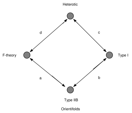
FIG. 1.: The relations between Type IIB orientifolds, Type I, heterotic and F-theory.

FIG. 2.: Open circles and dots represent the original Voisin–Borcea orbifolds. The line of $\otimes$’s corresponds to the extension discussed in section VIII.

Sector	Field	$SU(12)\otimes SO(8)\otimes U(1)$	Comments
Closed
Untwisted	$\phi_{ab}$	$9({\bf 1},{\bf 1})(0)_{L}$	$a,b=1,2,3$
Closed
Twisted	$S_{\alpha\beta\gamma}$	$27({\bf 1},{\bf 1})(0)_{L}$	$\alpha,\beta,\gamma=1,2,3$
Open	$Q_{a}$	$3({\bf 12},{\bf 8}_{v})(-1)_{L}$
	$\Phi_{a}$	$3({\overline{\bf 66}},{\bf 1})(+2)_{L}$	$a=1,2,3$

TABLE I.: The massless spectrum of the Type I ${\bf Z}_{3}$ orbifold model with $N=1$ space-time supersymmetry and gauge group $SU(12)\otimes SO(8)\otimes U(1)$ discussed in section IX. The gravity, dilaton and gauge supermultiplets are not shown.

Sector	Field	$SU(12)\otimes SO(8)\otimes U(1)$	Comments
	$\phi_{ab}$	$9({\bf 1},{\bf 1})(0)_{L}$	$a,b=1,2,3$
Untwisted	$Q_{a}$	$3({\bf 12},{\bf 8}_{v})(-1)_{L}$
	$\Phi_{a}$	$3({\overline{\bf 66}},{\bf 1})(+2)_{L}$
Twisted	$S_{\alpha\beta\gamma}$	$27({\bf 1},{\bf 1})(-4)_{L}$	$\alpha,\beta,\gamma=1,2,3$
	$T_{\alpha\beta\gamma}$	$27({\bf 1},{\bf 8}_{s})(+2)_{L}$

TABLE II.: The massless spectrum of the heterotic ${\bf Z}_{3}$ orbifold model with $N=1$ space-time supersymmetry and gauge group $SU(12)\otimes SO(8)\otimes U(1)$ discussed in section IX. The gravity, dilaton and gauge supermultiplets are not shown.

Sector	$[SU(6)\otimes SU(6)\otimes SU(4)\otimes U(1)^{3}]^{2}$	$(H_{1},H_{2},H_{3})_{-1}$	$(H_{1},H_{2},H_{3})_{-1/2}$
Closed
Untwisted	$5({\bf 1},{\bf 1},{\bf 1};{\bf 1},{\bf 1},{\bf 1})(0,0,0;0,0,0)_{L}$
Closed
${\bf Z}_{3}$ Twisted	$15({\bf 1},{\bf 1},{\bf 1};{\bf 1},{\bf 1},{\bf 1})(0,0,0;0,0,0)_{L}$
Closed
${\bf Z}_{6}$ Twisted	$3({\bf 1},{\bf 1},{\bf 1};{\bf 1},{\bf 1},{\bf 1})(0,0,0;0,0,0)_{L}$
Closed
${\bf Z}_{2}$ Twisted	$11({\bf 1},{\bf 1},{\bf 1};{\bf 1},{\bf 1},{\bf 1})(0,0,0;0,0,0)_{L}$
	$({\bf 15},{\bf 1},{\bf 1};{\bf 1},{\bf 1},{\bf 1})(+2,0,0;0,0,0)_{L}$	$(+1,0,0)$	$(+{1\over 2},-{1\over 2},-{1\over 2})$
	$({\bf 15},{\bf 1},{\bf 1};{\bf 1},{\bf 1},{\bf 1})(+2,0,0;0,0,0)_{L}$	$(0,+1,0)$	$(-{1\over 2},+{1\over 2},-{1\over 2})$
	$({\bf 1},\overline{\bf 15},{\bf 1};{\bf 1},{\bf 1},{\bf 1})(0,-2,0;0,0,0)_{L}$	$(+1,0,0)$	$(+{1\over 2},-{1\over 2},-{1\over 2})$
	$({\bf 1},\overline{\bf 15},{\bf 1};{\bf 1},{\bf 1},{\bf 1})(0,-2,0;0,0,0)_{L}$	$(0,+1,0)$	$(-{1\over 2},+{1\over 2},-{1\over 2})$
	$(\overline{\bf 6},{\bf 1},\overline{\bf 4};{\bf 1},{\bf 1},{\bf 1})(-1,0,-1;0,0,0)_{L}$	$(+1,0,0)$	$(+{1\over 2},-{1\over 2},-{1\over 2})$
	$(\overline{\bf 6},{\bf 1},\overline{\bf 4};{\bf 1},{\bf 1},{\bf 1})(-1,0,-1;0,0,0)_{L}$	$(0,+1,0)$	$(-{1\over 2},+{1\over 2},-{1\over 2})$
Open $99$	$({\bf 1},{\bf 6},{\bf 4};{\bf 1},{\bf 1},{\bf 1})(0,+1,+1;0,0,0)_{L}$	$(+1,0,0)$	$(+{1\over 2},-{1\over 2},-{1\over 2})$
	$({\bf 1},{\bf 6},{\bf 4};{\bf 1},{\bf 1},{\bf 1})(0,+1,+1;0,0,0)_{L}$	$(0,+1,0)$	$(-{1\over 2},+{1\over 2},-{1\over 2})$
	$({\bf 6},\overline{\bf 6},{\bf 1};{\bf 1},{\bf 1},{\bf 1})(+1,-1,0;0,0,0)_{L}$	$(0,0,+1)$	$(-{1\over 2},-{1\over 2},+{1\over 2})$
	$(\overline{\bf 6},{\bf 1},{\bf 4};{\bf 1},{\bf 1},{\bf 1})(-1,0,+1;0,0,0)_{L}$	$(0,0,+1)$	$(-{1\over 2},-{1\over 2},+{1\over 2})$
	$({\bf 1},{\bf 6},\overline{\bf 4};{\bf 1},{\bf 1},{\bf 1})(0,+1,-1;0,0,0)_{L}$	$(0,0,+1)$	$(-{1\over 2},-{1\over 2},+{1\over 2})$
	$({\bf 1},{\bf 1},{\bf 1};{\bf 15},{\bf 1},{\bf 1})(0,0,0;+2,0,0)_{L}$	$(+1,0,0)$	$(+{1\over 2},-{1\over 2},-{1\over 2})$
	$({\bf 1},{\bf 1},{\bf 1};{\bf 15},{\bf 1},{\bf 1})(0,0,0;+2,0,0)_{L}$	$(+1,0,0)$	$(+{1\over 2},-{1\over 2},-{1\over 2})$
	$({\bf 1},{\bf 1},{\bf 1};{\bf 1},\overline{\bf 15},{\bf 1})(0,0,0;0,-2,0)_{L}$	$(+1,0,0)$	$(+{1\over 2},-{1\over 2},-{1\over 2})$
	$({\bf 1},{\bf 1},{\bf 1};{\bf 1},\overline{\bf 15},{\bf 1})(0,0,0;0,-2,0)_{L}$	$(0,+1,0)$	$(-{1\over 2},+{1\over 2},-{1\over 2})$
	$({\bf 1},{\bf 1},{\bf 1};\overline{\bf 6},{\bf 1},\overline{\bf 4})(0,0,0;-1,0,-1)_{L}$	$(+1,0,0)$	$(+{1\over 2},-{1\over 2},-{1\over 2})$
	$({\bf 1},{\bf 1},{\bf 1};\overline{\bf 6},{\bf 1},\overline{\bf 4})(0,0,0;-1,0,-1)_{L}$	$(0,+1,0)$	$(-{1\over 2},+{1\over 2},-{1\over 2})$
Open $55$	$({\bf 1},{\bf 1},{\bf 1};{\bf 1},{\bf 6},{\bf 4})(0,0,0;0,+1,+1)_{L}$	$(+1,0,0)$	$(+{1\over 2},-{1\over 2},-{1\over 2})$
	$({\bf 1},{\bf 1},{\bf 1};{\bf 1},{\bf 6},{\bf 4})(0,0,0;0,+1,+1)_{L}$	$(0,+1,0)$	$(-{1\over 2},+{1\over 2},-{1\over 2})$
	$({\bf 1},{\bf 1},{\bf 1};{\bf 6},\overline{\bf 6},{\bf 1})(0,0,0;+1,-1,0)_{L}$	$(0,0,+1)$	$(-{1\over 2},-{1\over 2},+{1\over 2})$
	$({\bf 1},{\bf 1},{\bf 1};\overline{\bf 6},{\bf 1},{\bf 4})(0,0,0;-1,0,+1)_{L}$	$(0,0,+1)$	$(-{1\over 2},-{1\over 2},+{1\over 2})$
	$({\bf 1},{\bf 1},{\bf 1};{\bf 1},{\bf 6},\overline{\bf 4})(0,0,0;0,+1,-1)_{L}$	$(0,0,+1)$	$(-{1\over 2},-{1\over 2},+{1\over 2})$
	$({\bf 6},{\bf 1},{\bf 1};{\bf 6},{\bf 1},{\bf 1})(+1,0,0;+1,0,0)_{L}$	$(+{1\over 2},+{1\over 2},0)$	$(0,0,-{1\over 2})$
	$({\bf 1},{\bf 6},{\bf 1};{\bf 1},{\bf 1},{\bf 4})(0,+1,0;0,0,+1)_{L}$	$(+{1\over 2},+{1\over 2},0)$	$(0,0,-{1\over 2})$
Open $59$	$({\bf 1},{\bf 1},{\bf 4};{\bf 1},{\bf 6},{\bf 1})(0,0,+1;0,+1,0)_{L}$	$(+{1\over 2},+{1\over 2},0)$	$(0,0,-{1\over 2})$
	$(\overline{\bf 6},{\bf 1},{\bf 1};{\bf 1},{\bf 1},\overline{\bf 4})(-1,0,0;0,0,-1)_{L}$	$(+{1\over 2},+{1\over 2},0)$	$(0,0,-{1\over 2})$
	$({\bf 1},\overline{\bf 6},{\bf 1};{\bf 1},\overline{\bf 6},{\bf 1})(0,-1,0;0,-1,0)_{L}$	$(+{1\over 2},+{1\over 2},0)$	$(0,0,-{1\over 2})$
	$({\bf 1},{\bf 1},\overline{\bf 4};\overline{\bf 6},{\bf 1},{\bf 1})(0,0,-1;-1,0,0)_{L}$	$(+{1\over 2},+{1\over 2},0)$	$(0,0,-{1\over 2})$

TABLE III.: The massless spectrum of the type I ${\bf Z}_{6}$ orbifold model with $N=1$ space-time supersymmetry and gauge group $[SU(6)\otimes SU(6)\otimes SU(4)\otimes U(1)^{3}]^{2}$ discussed in section X. The $H$-charges in both the $-1$ picture and the $-1/2$ picture for states in the open string sector are also given. The gravity, dilaton and gauge supermultiplets are not shown.

Sector	$[SU(8)\otimes SU(8)\otimes U(1)^{2}]^{2}$	$(H_{1},H_{2},H_{3})_{-1}$	$(H_{1},H_{2},H_{3})_{-1/2}$
Closed	$6({\bf 1},{\bf 1},{\bf 1};{\bf 1},{\bf 1},{\bf 1})(0,0,0;0,0,0)_{L}$
Untwisted
Closed	$16({\bf 1},{\bf 1},{\bf 1};{\bf 1},{\bf 1},{\bf 1})(0,0,0;0,0,0)_{L}$
${\bf Z}_{4}$ Twisted
Closed	$16({\bf 1},{\bf 1},{\bf 1};{\bf 1},{\bf 1},{\bf 1})(0,0,0;0,0,0)_{L}$
${\bf Z}_{2}$ Twisted
	$({\bf 8},\overline{\bf 8};{\bf 1},{\bf 1})(+1,-1;0,0)_{L}$	$(+1,0,0)$	$(+{1\over 2},-{1\over 2},-{1\over 2})$
	$(\overline{\bf 28},{\bf 1};{\bf 1},{\bf 1})(-2,0;0,0)_{L}$	$(+1,0,0)$	$(+{1\over 2},-{1\over 2},-{1\over 2})$
	$({\bf 1},{\bf 28};{\bf 1},{\bf 1})(0,+2;0,0)_{L}$	$(+1,0,0)$	$(+{1\over 2},-{1\over 2},-{1\over 2})$
Open $99$	$({\bf 8},\overline{\bf 8};{\bf 1},{\bf 1})(+1,-1;0,0)_{L}$	$(0,+1,0)$	$(-{1\over 2},+{1\over 2},-{1\over 2})$
	$(\overline{\bf 28},{\bf 1};{\bf 1},{\bf 1})(-2,0;0,0)_{L}$	$(0,+1,0)$	$(-{1\over 2},+{1\over 2},-{1\over 2})$
	$({\bf 1},{\bf 28};{\bf 1},{\bf 1})(0,+2;0,0)_{L}$	$(0,+1,0)$	$(-{1\over 2},+{1\over 2},-{1\over 2})$
	$({\bf 8},{\bf 8};{\bf 1},{\bf 1})(+1,+1;0,0)_{L}$	$(0,0,+1)$	$(-{1\over 2},-{1\over 2},+{1\over 2})$
	$(\overline{\bf 8},\overline{\bf 8};{\bf 1},{\bf 1})(-1,-1;0,0)_{L}$	$(0,0,+1)$	$(-{1\over 2},-{1\over 2},+{1\over 2})$
	$({\bf 1},{\bf 1};{\bf 8},\overline{\bf 8})(0,0;+1,-1)_{L}$	$(+1,0,0)$	$(+{1\over 2},-{1\over 2},-{1\over 2})$
	$({\bf 1},{\bf 1};\overline{\bf 28},{\bf 1})(0,0;-2,0)_{L}$	$(+1,0,0)$	$(+{1\over 2},-{1\over 2},-{1\over 2})$
	$({\bf 1},{\bf 1};{\bf 1},{\bf 28})(0,0;0,+2)_{L}$	$(+1,0,0)$	$(+{1\over 2},-{1\over 2},-{1\over 2})$
Open $55$	$({\bf 1},{\bf 1};{\bf 8},\overline{\bf 8})(0,0;+1,-1)_{L}$	$(0,+1,0)$	$(-{1\over 2},+{1\over 2},-{1\over 2})$
	$({\bf 1},{\bf 1};\overline{\bf 28},{\bf 1})(0,0;-2,0)_{L}$	$(0,+1,0)$	$(-{1\over 2},+{1\over 2},-{1\over 2})$
	$({\bf 1},{\bf 1};{\bf 1},{\bf 28})(0,0;0,+2)_{L}$	$(0,+1,0)$	$(-{1\over 2},+{1\over 2},-{1\over 2})$
	$({\bf 1},{\bf 1};{\bf 8},{\bf 8})(0,0;+1,+1)_{L}$	$(0,0,+1)$	$(-{1\over 2},-{1\over 2},+{1\over 2})$
	$({\bf 1},{\bf 1};\overline{\bf 8},\overline{\bf 8})(0,0;-1,-1)_{L}$	$(0,0,+1)$	$(-{1\over 2},-{1\over 2},+{1\over 2})$
	$(\overline{\bf 8},{\bf 1};\overline{\bf 8},{\bf 1})(-1,0;-1,0)_{L}$	$(+{1\over 2},+{1\over 2},0)$	$(0,0,-{1\over 2})$
Open $59$	$({\bf 1},{\bf 8};{\bf 1},{\bf 8})(0,+1;0,+1)_{L}$	$(+{1\over 2},+{1\over 2},0)$	$(0,0,-{1\over 2})$
	$({\bf 8},{\bf 1};{\bf 1},{\overline{\bf 8}})(+1,0;0,-1)_{L}$	$(+{1\over 2},+{1\over 2},0)$	$(0,0,-{1\over 2})$
	$({\bf 1},{\overline{\bf 8}};{\bf 8},{\bf 1})(0,-1;+1,0)_{L}$	$(+{1\over 2},+{1\over 2},0)$	$(0,0,-{1\over 2})$

TABLE IV.: The perturbative (from the orientifold viewpoint) massless spectrum of the four dimensional ${\cal N}=1$ space-time supersymmetric orientifold of Type IIB on $T^{6}/{\bf Z}_{4}$ orbifold discussed in section XI. The gauge group is $[U(8)\otimes U(8)]_{99}\otimes[U(8)\otimes U(8)]_{55}$. The $H$-charges in both the $-1$ picture and the $-1/2$ picture for states in the open string sectors are also given. The gravity, dilaton and gauge supermultiplets are not shown.

Sector	$[SU(4)\otimes SU(4)\otimes SU(8)\otimes U(1)^{3}]^{2}$	$(H_{1},H_{2},H_{3})_{-1}$	$(H_{1},H_{2},H_{3})_{-1/2}$
Closed
Untwisted	$4({\bf 1},{\bf 1},{\bf 1};{\bf 1},{\bf 1},{\bf 1})(0,0,0;0,0,0)_{L}$
Closed
${\bf Z}_{3}$ Twisted	$18({\bf 1},{\bf 1},{\bf 1};{\bf 1},{\bf 1},{\bf 1})(0,0,0;0,0,0)_{L}$
Closed
${\bf Z}_{6}$ Twisted	$12({\bf 1},{\bf 1},{\bf 1};{\bf 1},{\bf 1},{\bf 1})(0,0,0;0,0,0)_{L}$
Closed
${\bf Z}_{2}$ Twisted	$12({\bf 1},{\bf 1},{\bf 1};{\bf 1},{\bf 1},{\bf 1})(0,0,0;0,0,0)_{L}$
	$(\overline{\bf 4},{\bf 1},{\bf 8};{\bf 1},{\bf 1},{\bf 1})(-1,0,+1;0,0,0)_{L}$	$(0,0,+1)$	$(-{1\over 2},-{1\over 2},+{1\over 2})$
	$({\bf 1},{\bf 4},\overline{\bf 8};{\bf 1},{\bf 1},{\bf 1})(0,+1,-1;0,0,0)_{L}$	$(0,0,+1)$	$(-{1\over 2},-{1\over 2},+{1\over 2})$
	$({\bf 4},\overline{\bf 4},{\bf 1};{\bf 1},{\bf 1},{\bf 1})(+1,-1,0;0,0,0)_{L}$	$(0,0,+1)$	$(-{1\over 2},-{1\over 2},+{1\over 2})$
	$({\bf 4},{\bf 1},{\bf 8};{\bf 1},{\bf 1},{\bf 1})(+1,0,+1;0,0,0)_{L}$	$(0,+1,0)$	$(-{1\over 2},+{1\over 2},-{1\over 2})$
	$({\bf 1},\overline{\bf 4},\overline{\bf 8};{\bf 1},{\bf 1},{\bf 1})(0,-1,-1;0,0,0)_{L}$	$(0,+1,0)$	$(-{1\over 2},+{1\over 2},-{1\over 2})$
Open $99$	$({\bf 6},{\bf 1},{\bf 1};{\bf 1},{\bf 1},{\bf 1})(-2,0,0;0,0,0)_{L}$	$(0,+1,0)$	$(-{1\over 2},+{1\over 2},-{1\over 2})$
	$({\bf 1},{\bf 6},{\bf 1};{\bf 1},{\bf 1},{\bf 1})(0,+2,0;0,0,0)_{L}$	$(0,+1,0)$	$(-{1\over 2},+{1\over 2},-{1\over 2})$
	$({\bf 1},{\bf 1},{\bf 28};{\bf 1},{\bf 1},{\bf 1})(0,0,+2;0,0,0)_{L}$	$(+1,0,0)$	$(+{1\over 2},-{1\over 2},-{1\over 2})$
	$({\bf 1},{\bf 1},\overline{\bf 28};{\bf 1},{\bf 1},{\bf 1})(0,0,-2;0,0,0)_{L}$	$(+1,0,0)$	$(+{1\over 2},-{1\over 2},-{1\over 2})$
	$({\bf 4},{\bf 4},{\bf 1};{\bf 1},{\bf 1},{\bf 1})(+1,+1,0;0,0,0)_{L}$	$(+1,0,0)$	$(+{1\over 2},-{1\over 2},-{1\over 2})$
	$(\overline{\bf 4},\overline{\bf 4},{\bf 1};{\bf 1},{\bf 1},{\bf 1})(-1,-1,0;0,0,0)_{L}$	$(+1,0,0)$	$(+{1\over 2},-{1\over 2},-{1\over 2})$
	$({\bf 1},{\bf 1},{\bf 1};\overline{\bf 4},{\bf 1},{\bf 8})(0,0,0;-1,0,+1)_{L}$	$(0,0,+1)$	$(-{1\over 2},-{1\over 2},+{1\over 2})$
	$({\bf 1},{\bf 1},{\bf 1};{\bf 1},{\bf 4},\overline{\bf 8})(0,0,0;0,+1,-1)_{L}$	$(0,0,+1)$	$(-{1\over 2},-{1\over 2},+{1\over 2})$
	$({\bf 1},{\bf 1},{\bf 1};{\bf 4},\overline{\bf 4},{\bf 1})(0,0,0;+1,-1,0)_{L}$	$(0,0,+1)$	$(-{1\over 2},-{1\over 2},+{1\over 2})$
	$({\bf 1},{\bf 1},{\bf 1};{\bf 4},{\bf 1},{\bf 8})(0,0,0;+1,0,+1)_{L}$	$(0,+1,0)$	$(-{1\over 2},+{1\over 2},-{1\over 2})$
	$({\bf 1},{\bf 1},{\bf 1};{\bf 1},\overline{\bf 4},\overline{\bf 8})(0,0,0;0,-1,-1)_{L}$	$(0,+1,0)$	$(-{1\over 2},+{1\over 2},-{1\over 2})$
Open $55$	$({\bf 1},{\bf 1},{\bf 1};{\bf 6},{\bf 1},{\bf 1})(0,0,0;-2,0,0)_{L}$	$(0,+1,0)$	$(-{1\over 2},+{1\over 2},-{1\over 2})$
	$({\bf 1},{\bf 1},{\bf 1};{\bf 1},{\bf 6},{\bf 1})(0,0,0;0,+2,0)_{L}$	$(0,+1,0)$	$(-{1\over 2},+{1\over 2},-{1\over 2})$
	$({\bf 1},{\bf 1},{\bf 1};{\bf 1},{\bf 1},{\bf 28})(0,0,0;0,0,+2)_{L}$	$(+1,0,0)$	$(+{1\over 2},-{1\over 2},-{1\over 2})$
	$({\bf 1},{\bf 1},{\bf 1};{\bf 1},{\bf 1},\overline{\bf 28})(0,0,0;0,0,-2)_{L}$	$(+1,0,0)$	$(+{1\over 2},-{1\over 2},-{1\over 2})$
	$({\bf 1},{\bf 1},{\bf 1};{\bf 4},{\bf 4},{\bf 1})(0,0,0;+1,+1,0)_{L}$	$(+1,0,0)$	$(+{1\over 2},-{1\over 2},-{1\over 2})$
	$({\bf 1},{\bf 1},{\bf 1};\overline{\bf 4},\overline{\bf 4},{\bf 1})(0,0,0;-1,-1,0)_{L}$	$(+1,0,0)$	$(+{1\over 2},-{1\over 2},-{1\over 2})$
	$({\bf 4},{\bf 1},{\bf 1};{\bf 4},{\bf 1},{\bf 1})(+1,0,0;+1,0,0)_{L}$	$(+{1\over 2},+{1\over 2},0)$	$(0,0,-{1\over 2})$
	$({\bf 1},{\bf 4},{\bf 1};{\bf 1},{\bf 1},{\bf 8})(0,+1,0;0,0,+1)_{L}$	$(+{1\over 2},+{1\over 2},0)$	$(0,0,-{1\over 2})$
Open $59$	$({\bf 1},{\bf 1},{\bf 8};{\bf 1},{\bf 4},{\bf 1})(0,0,+1;0,+1,0)_{L}$	$(+{1\over 2},+{1\over 2},0)$	$(0,0,-{1\over 2})$
	$(\overline{\bf 4},{\bf 1},{\bf 1};{\bf 1},{\bf 1},\overline{\bf 8})(-1,0,0;0,0,-1)_{L}$	$(+{1\over 2},+{1\over 2},0)$	$(0,0,-{1\over 2})$
	$({\bf 1},\overline{\bf 4},{\bf 1};{\bf 1},\overline{\bf 4},{\bf 1})(0,-1,0;0,-1,0)_{L}$	$(+{1\over 2},+{1\over 2},0)$	$(0,0,-{1\over 2})$
	$({\bf 1},{\bf 1},\overline{\bf 8};\overline{\bf 4},{\bf 1},{\bf 1})(0,0,-1;-1,0,0)_{L}$	$(+{1\over 2},+{1\over 2},0)$	$(0,0,-{1\over 2})$

TABLE V.: The perturbative (from the orientifold viewpoint) massless spectrum of the four dimensional ${\cal N}=1$ space-time supersymmetric orientifold of Type IIB on $T^{6}/{\bf Z}_{6}^{\prime}$ orbifold discussed in section XI. The gauge group is $[U(4)\otimes U(4)\otimes U(8)]_{99}\otimes[U(4)\otimes U(4)\otimes U(8)]_{55}$. The $H$-charges in both the $-1$ picture and the $-1/2$ picture for states in the open string sectors are also given. The gravity, dilaton and gauge supermultiplets are not shown.

REFERENCES

- [1] J. Polchinski, Phys. Rev. Lett. 75 (1995) 4724.
- [2] C.G. Callan, C. Lovelace, C.R. Nappi, S.A. Yost, Nucl. Phys. B293 (1987) 83; Nucl. Phys. B308 (1988) 221.
- [3] J. Polchinski and Y. Cai, Nucl. Phys. B296 (1988) 91.
- [4] N. Ishibashi and T. Onogi, Nucl. Phys. B318 (1989) 239.
-
[5]
D.C. Dunbar, Nucl. Phys. B319 (1989) 72;
Z. Bern and D.C. Dunbar, Nucl. Phys. B319 (1989) 104. -
[6]
S.M. Roy and V. Singh, Phys. Rev. D35 (1987) 1939;
Phys. Rev. D36 (1987) 1827;
P.Horava, Nucl. Phys. B327 (1989) 461; Phys. Lett. B231 (1989) 251;
J. Dai, R.G. Leigh and J. Polchinski, Mod. Phys. Lett. A4 (1989) 2073;
R.G. Leigh, Mod. Phys. Lett. A4 (1989) 2767. -
[7]
G. Pradisi and A. Sagnotti, Phys. Lett. B216 (1989) 59;
M. Bianchi and A. Sagnotti, Phys. Lett. B247 (1990) 517; Nucl. Phys. B361 (1991) 539. - [8] E.G. Gimon and J. Polchinski, Phys. Rev. D54 (1996) 1667, hep-th/9601038.
- [9] E.G. Gimon and C.V. Johnson, Nucl. Phys. B477 (1996) 715, hep-th/9604129.
- [10] A. Dabholkar and J. Park, Nucl. Phys. B477 (1996) 701, hep-th/9604178.
- [11] J. Polchinski and E. Witten, Nucl. Phys. B460 (1996) 525, hep-th/9510169.
- [12] M. Berkooz and R.G. Leigh, Nucl. Phys. B483 (1997) 187, hep-th/9605049.
- [13] C. Angelantonj, M. Bianchi, G. Pradisi, A. Sagnotti and Ya.S. Stanev, Phys. Lett. B385 (1996) 96, hep-th/9606169.
- [14] Z. Kakushadze, Nucl. Phys. B512 (1998) 221, hep-th/9704059.
- [15] Z. Kakushadze and G. Shiu, Phys. Rev. D56 (1997) 3686, hep-th/9705163.
- [16] Z. Kakushadze and G. Shiu, hep-th/9706051.
- [17] G. Zwart, hep-th/9708040.
- [18] G. Aldazabal, A. Font, L.E. Ibáñez and G. Violero, hep-th/9804026.
- [19] Z. Kakushadze, hep-th/9804110.
- [20] A. Sen, Phys. Rev. D55 (1997) 7345, hep-th/9702165; hep-th/9709159.
- [21] C. Vafa, Nucl. Phys. B469 (1996) 403, hep-th/9602022.
- [22] E.G. Gimon and C.V. Johnson, Nucl. Phys. B479 (1996) 285, hep-th/9606176.
- [23] P. Berglund and E.G. Gimon, hep-th/9803168.
- [24] C. Voisin, in: Journeés de Géométrie Algébrique d’Orsay, eds. A. Beauville et al., Astérisque, vol. 218 (Soc. Math. France, 1993) 273-323.
- [25] C. Borcea, in: Mirror Manifolds II, eds. B.R. Greene and S.-T. Yau (International Press and AMS, 1997) 717-743.
- [26] L. Dixon, J. Harvey, C. Vafa and E. Witten, Nucl. Phys. B261 (1985) 678; Nucl. Phys. B274 (1986) 285.
- [27] A. Dabholkar and J. Park, Nucl. Phys. B472 (1996) 207, hep-th/9602030.
- [28] J. Polchinski, Phys. Rev. D55 (1997) 6423, hep-th/9606165.
- [29] J.D. Blum, Nucl. Phys. B486 (1997) 34, hep-th/9608053.
- [30] V.V. Nikulin, in: Proc. ICM (Berkeley, 1986) 654-671.
- [31] D.R. Morrison and C. Vafa, Nucl. Phys. B473 (1996) 74, hep-th/9602114; Nucl. Phys. B476 (1996) 437, hep-th/9603161.
- [32] S. Sethi, C. Vafa and E. Witten, Nucl. Phys. B480 (1996) 213, hep-th/9606122.
- [33] R. Gopakumar and S. Mukhi, Nucl. Phys. B479 (1996) 260, hep-th/9607057.
-
[34]
R. Friedman, J. Morgan and E. Witten, Commun. Math. Phys.
187 (1997),
hep-th/9701162;
M. Bershadsky, A. Johansen, T. Pantev and V. Sadov, Nucl. Phys. B505 (1997) 165, hep-th/9701165. -
[35]
See, e.g.,
I. Brunner and R. Schimmrigk, Phys. Lett. B387 (1996) 750, hep-th/9606148;
A. Klemm, B. Lian, S.-S. Roan and S.-T. Yau, hep-th/9701021;
K. Mohri, hep-th/9701147;
R. Friedman, J. Morgan and E. Witten, alg-geom/9707004; alg-geom/9709029;
M. Bershadsky and V. Sadov, hep-th/9703194;
A. Grassi, alg-geom/9704008;
M. Bershadsky, T.-M. Chiang, B.R. Greene, A. Johansen and C.I. Lazaroiu, hep-th/9712023;
G. Curio and R.Y. Donagi, hep-th/9801058;
R. Donagi, hep-th/9802093; hep-th/9802094. - [36] M.R. Douglas and G. Moore, hep-th/9603167.
- [37] P.S. Aspinwall, Phys. Lett. B357 (1995) 329, hep-th/9507012.
- [38] M. Berkooz, R.G. Leigh, J. Polchinski, J.H. Schwarz, N. Seiberg and E. Witten, Nucl. Phys. B475 (1996) 115, hep-th/9605184.
- [39] A. Sen, Nucl. Phys. B489 (1997) 139, hep-th/9611186; Nucl. Phys. B498 (1997) 135, hep-th/9702061.
- [40] J. Blum and A. Zaffaroni, Phys. Lett. B387 (1996) 71, hep-th/9607019.
- [41] A. Dabholkar and J. Park, Phys. Lett. B394 (1997) 302, hep-th/9607041.
- [42] G. Aldazabal, A. Font, L.E. Ibáñez, A.M. Uranga and G. Violero, hep-th/9706158.
- [43] D. O’Driscoll, hep-th/9801114.
- [44] Z. Kakushadze, hep-th/9803214.
- [45] P.S. Aspinwall, Nucl. Phys. B460 (1996) 57, hep-th/9510142.
- [46] Z. Kakushadze, G. Shiu and S.-H.H. Tye, hep-th/9803141.
- [47] C. Vafa and E. Witten, J. Geom. Phys. 15 (1995) 189, hep-th/9409188.
-
[48]
S. Chaudhuri, G. Hockney and J.D. Lykken, Phys. Rev. Lett. 75 (1995) 2264,
hep-th/9505054;
S. Chaudhuri and J. Polchinski, Phys. Rev. D52 (1995) 7168, hep-th/9506048. -
[49]
I. Antoniadis, C. Bachas, C. Fabre, H. Partouche and T.R. Taylor,
Nucl. Phys. B489 (1997) 160, hep-th/9608012;
I. Antoniadis, H. Partouche and T.R. Taylor, Nucl. Phys. Proc. Suppl. 61A (1998) 58, hep-th/9706211. - [50] A. Sen and S. Sethi, Nucl. Phys. B499 (1997) 45, hep-th/9703157.
- [51] C. Angelantonj and G. Pradisi, preprint ROM2F-97/41, unpublished.
- [52] Z. Kakushadze, hep-th/9804184.