N=8 gaugings revisited :
an exhaustive classification^∗†
Francesco Cordaro¹, Pietro Fré¹, Leonardo Gualtieri¹,
Piet Termonia¹, and Mario Trigiante²

¹ Dipartimento di Fisica Teorica, Universitá di Torino, via P. Giuria 1, I-10125 Torino,
Istituto Nazionale di Fisica Nucleare (INFN) - Sezione di Torino, Italy
² Department of Physics, University of Wales Swansea, Singleton Park,
Swansea SA2 8PP, United Kingdom

Abstract

In this paper we reconsider, for $N=8$ supergravity, the problem of gauging the most general electric subgroup. We show that admissible theories are fully characterized by a single algebraic equation to be satisfied by the embedding ${\cal G}_{gauge}\rightarrow SL(8,{\rm I\kern-1.61993ptR})\subset E_{7(7)}$. The complete set of solutions to this equation contains $36$ parameters. Modding by the action of $SL(8,{\rm I\kern-1.61993ptR})$ conjugations that yield equivalent theories all continuous parameters are eliminated except for an overall coupling constant and we obtain a discrete set of orbits. This set is in one–to–one correspondence with $36$ Lie subalgebras of $SL(8,{\rm I\kern-1.61993ptR})$, corresponding to all possible real forms of the $SO(8)$ Lie algebra plus a set of contractions thereof. By means of our analysis we establish the theorem that the N=8 gaugings constructed by Hull in the middle eighties constitute the exhaustive set of models. As a corollary we show that there exists a unique $7$–dimensional abelian gauging. The corresponding abelian algebra is not contained in the maximal abelian ideal of the solvable Lie algebra generating the scalar manifold $E_{7(7)}/SU(8)$  ^∗ Supported in part by EEC under TMR contract ERBFMRX-CT96-0045
^† Supported in part by EEC under TMR contract ERBFMRXCT960012, in which M. Trigiante is associated to Swansea University

1 Introduction

Supergravity theory was developed in the late seventies and in the early eighties in a completely independent way from string theory. Yet it has proved to encode a surprising wealth of non perturbative information about the various superstrings and the candidate microscopic theory that unifies all of them: M–theory. [1, 2] Most prominent about the features of supergravity models that teach us something about non perturbative string states is the U–duality group, namely the isometry group of the scalar sector whose discrete subgroup $U(\mathchoice{\hbox{\cmss Z\kern-3.99994ptZ}}{\hbox{\cmss Z\kern-3.99994ptZ}}{\lower 0.9pt\hbox{\cmsss Z\kern-2.79996ptZ}}{\lower 1.2pt\hbox{\cmsss Z\kern-2.79996ptZ}})$ is believed to be an exact symmetry of the non–perturbative string spectrum [1]. This viewpoint has been successfully applied to the construction of BPS saturated $p$–brane solutions that provide the missing partners of perturbative string states needed to complete U–duality multiplets [3, 4]. In particular in space–time dimension $D=4$ an active study has been performed of BPS $0$–branes, namely extremal black–holes, for extended supergravities with $2\leq N\leq 8$ [5, 6, 7, 8]. These non–perturbative quantum states are described by classical solutions of the ungauged version of supergravity which in the first two years after the second string revolution [1, 2] has been the focus of attention of string theorists. Ungauged supergravity corresponds to the case where the maximal symmetric solution is Minkowski space $M^{Mink}_{D}$ and furthermore no field in the theory is charged with respect to the vector fields, in particular the graviphotons.

Another aspect of supergravity that has recently received renewed attention is its gauging. Gauged supergravity corresponds to the situation where the maximal symmetric solution is not necessarily Minkowski space but can also be anti–de Sitter space $AdS_{D}$ and where fields are charged with respect to the vectors present in the theory, in particular the graviphotons (for a review see [9]). In gauged supergravity three modifications occur:

1. A subgroup $G_{gauge}\subset G_{elect}\subset U$ is gauged, namely becomes a local symmetry. $G_{elect}$ is by definition the subgroup of the U–duality group that maps the set of electric field strengths into itself without mixing them with the magnetic ones. As a consequence U–duality is classically broken and only its discrete part $U(\mathchoice{\hbox{\cmss Z\kern-3.99994ptZ}}{\hbox{\cmss Z\kern-3.99994ptZ}}{\lower 0.9pt\hbox{\cmsss Z\kern-2.79996ptZ}}{\lower 1.2pt\hbox{\cmsss Z\kern-2.79996ptZ}})$ can survive non–perturbatively.

2. The supersymmetry transformation rules are modified through the addition of non–derivative terms that depend only on the scalar fields and that are usually named the fermion shifts $\Sigma_{A}^{i}(\phi)$. Namely we have:

   $$\delta\mbox{fermion}^{i}=\dots\,+\,\Sigma_{A}^{i}(\phi)\,\epsilon^{A}$$ (1)

3. A scalar potential ${\cal V}(\phi)$ is generated that is related to the fermion shifts by a bilinear Ward identity [10]

   $$\delta_{A}^{B}\,{\cal V}(\phi)\,=\,\Sigma_{A}^{i}(\phi)\,\Sigma^{Bj}(\phi)\,M_{ij}$$ (2)

   where $M_{ij}$ is a suitable constant matrix depending on the specific supergravity model considered and where the lower and upper capital latin indices $A,B,\dots$ enumerate the left and right chiral projection of the supersymmetry charges, respectively.

Recently it has been verified [11, 7, 12] that one can construct $Mp$–brane and $Dp$–brane solutions of either D=11 [13, 14] or type IIB D=10 supergravity [15] with the following property: near the horizon their structure is described by a gauged supergravity theory in dimension $d=p+2$ and the near horizon geometry [16] is:

$${\cal M}^{h}=AdS_{p+2}\,\times\,{M}_{D-p-2}$$ (3)

$AdS_{p+2}$ being a notation for anti–de Sitter space and ${M}_{D-p-2}$ denoting an Einstein manifold in the complementary dimensions. Hence near the horizon one has a Kaluza–Klein expansion on ${M}_{D-p-2}$ whose truncation to zero–modes is gauged supergravity, the extension $N$ being decided by the number of Killing spinors admitted by ${M}_{D-p-2}$ and the group $G_{gauge}$ that is gauged being related to the isometry group $G_{iso}$ of this manifold. For instance the simplest example of $M2$ brane flows at the horizon to the geometry

$${\cal M}^{h}=AdS_{4}\,\times\,{S}^{7}$$ (4)

and in that region it is described by the $SO(8)$ gauging of $N=8$ supergravity, namely the de Wit and Nicolai theory [17]. Furthermore, as it is extensively discussed in recent literature one finds a duality between Kaluza–Klein supergravity yielding the gauged model and the conformal field theory on the world volume describing the microscopic degrees of freedom of the quantum brane.

In view of this relation an important problem that emerges is that of determining the precise relation between the various possible gaugings of the same ungauged supergravity theory and the near horizon geometry of various branes. In this paper we do not attempt to solve such a problem but we have it as a clear motivation for our revisitation of the problem we actually address: the classification of all possible gaugings for $N=8$ supergravity.

Another reason for revisiting the gauging problem comes from the lesson taught us by the $N=2$ case. In [18], extending work of [19], we discovered that $N=2$ supersymmetry can be spontaneously broken to $N=1$ when the following conditions are met:

• The scalar manifold of supergravity, which is generically given by the direct product ${\cal SK}\otimes{\cal QK}$ of a special Kähler manifold with a quaternionic one, is a homogeneous non–compact coset manifold ${\cal G}/{\cal H}$

• Some translational abelian symmetries of ${\cal G}/{\cal H}$ are gauged.

The basic ingredient in deriving the above result is the Alekseevskian description [20] of the scalar manifold ${\cal SK}\otimes{\cal QK}$ in terms of solvable Lie algebras, a Kähler algebra ${\cal K}$ for the vector multiplet sector ${\cal SK}$ and a quaternionic algebra ${\cal Q}$ for the hypermultiplet sector ${\cal QK}$. By means of this description the homogeneous non compact coset manifold ${\cal G}/{\cal H}$ is identified with the solvable group manifold $\exp[Solv]$ where

$$Solv={\cal K}\,\oplus\,{\cal Q}$$ (5)

and the translational symmetries responsible for the supersymmetry breaking are identified with suitable abelian subalgebras

$${\cal T}\,\subset\,Solv$$ (6)

An obvious observation that easily occurs once such a perspective is adopted is the following one: for all extended supergravities with $N\geq 3$ the scalar manifold is a homogeneous non–compact coset manifold ${\cal G}/{\cal H}$. Hence it was very tempting to extend the solvable Lie algebra approach to such supergravity theories, in particular to the maximal extended ones in all dimensions $4\leq D\leq 10$. This is what was done in the series of three papers [21, 22, 8]. Relying on a well established mathematical theory which is available in standard textbooks (for instance [23]), every non–compact homogeneous space ${\cal G}/{\cal H}$ is a solvable group manifold and its generating solvable Lie algebra $Solv\left({\cal G}/{\cal H}\right)$ can be constructed utilizing roots and Dynkin diagram techniques. This fact offers the so far underestimated possibility of introducing an intrinsic algebraic characterization of the supergravity scalars. In relation with string theory this yields a group–theoretical definition of Ramond and Neveu–Schwarz scalars. In the case of $N=8$ supergravity the scalar coset manifold $E_{7(7)}/SU(8)$ is generated by a solvable Lie algebra with the following structure:

$$Solv(E_{7(7)})={\cal H}_{7}\oplus\Phi^{+}(E_{7})$$ (7)

where ${\cal H}_{7}$ is the Cartan subalgebra and where $\Phi^{+}(E_{7})$ is the $63$ dimensional positive part of the $E_{7}$ root space. As shown in [22] this latter admits the decomposition:

$$\Phi^{+}(E_{7})=\Phi^{+}(E_{2})\oplus{\rm I\kern-1.79993ptD}^{+}_{2}\oplus{\rm I\kern-1.79993ptD}^{+}_{3}\oplus{\rm I\kern-1.79993ptD}^{+}_{4}\oplus{\rm I\kern-1.79993ptD}^{+}_{5}\oplus{\rm I\kern-1.79993ptD}^{+}_{6}$$ (8)

where $\Phi^{+}(E_{2})$ is the one–dimensional root space of the U–duality group in $D=9$ and ${\rm I\kern-1.79993ptD}^{+}_{r+1}={\cal A}_{r+2}$ the maximal abelian ideal of the U–duality solvable Lie algebra in $D=10-r-1$ dimensions. In particular for the $N=8,D=4$ theory the maximal abelian ideal of the solvable Lie algebra is:

$$\begin{array}[]{rclcl}\mbox{max. abel. ideal}&\rightarrow&{\cal A}_{7}&\equiv&{\rm I\kern-1.79993ptD}^{+}_{6}\subset Solv(E_{7(7)})\cr\mbox{dim}{\cal A}_{7}&=&27&\hbox{}\hfil&\hbox{}\cr\end{array}$$ (9)

Therefore, relying on the experience gained in the context of the $N=2$ case in [22] we have considered the possible gauging of an abelian subalgebra ${\cal A}_{gauge}$ within this maximal abelian ideal. In this context by maximal we refer to the property of having maximal dimension. It was reasonable to expect that such a gauging might produce a spontaneous breaking of supersymmetry with flat directions just as it happened in the lower supersymmetry example. The basic consistency criterion to gauge an $n$–dimensional subgroup of the translational symmetries is that we find at least $n$ vectors which are inert under the action of the proposed subalgebra. Indeed the set of vectors that can gauge an abelian algebra (being in its adjoint representation) must be neutral under the action of such an algebra. In [22], applying this criterion we found that the gaugeable subalgebra of the maximal abelian ideal is $7$–dimensional.

$$7=\mbox{dim}{\cal A}_{gaugeable}\,\subset\,{\cal A}_{7}\,\subset\,Solv(E_{7(7)})$$ (10)

Yet this was only a necessary but not sufficient criterion for the existence of the gauging. So whether translationally isometries of the solvable Lie algebra could be gauged was not established in [22].

The present paper provides an answer to this question and the answer is negative. Namely, we derive an algebraic equation that yields a necessary and sufficient condition for $N=8$ gaugings and we obtain the complete set of its solutions. This leads to an exhaustive classifications of all gauged $N=8$ supergravities. The set we obtain coincides with the set of gauged models obtained more than ten years ago by Hull [24] whose completeness was not established, so far. In the classification there appears a unique abelian gauging and in this case the gauged Lie algebra is indeed $7$–dimensional. However this abelian algebra, named $CSO(1,7)$ in Hull’s terminology is not contained in the maximal abelian ideal ${\cal A}_{7}$ since one of its elements belongs to ${\rm I\kern-1.79993ptD}_{5}^{+}$.

So a question that was left open in [22] is answered by the present paper.

Having established the result we present in this paper the next step that should be addressed is the study of critical points for all the classified gaugings, their possible relation with $p$–brane solutions and with partial supersymmetry breaking possibly in $AdS_{4}$, rather than in Minkowski space. Such a program will be undertaken elsewhere.

The rest of the paper is devoted to proving the result we have described.

2 N=8 Gauged Supergravity

In this section we summarize the structure of gauged N=8 supergravity and we pose the classification problem we have solved.

2.1 The bosonic lagrangian

According to the normalizations of [25] and [8] the bosonic Lagrangian of gauged N=8 supergravity has the following form:

$$\begin{array}[]{ccl}{\cal L}&=&\sqrt{-g}\,\Bigl{(}2\,R[g]+\frac{1}{4}\,\mbox{Im}\,{\cal N}_{\Lambda\Sigma,\Delta\Pi}\,{\cal F}^{\Lambda\Sigma|\mu\nu}\,{\cal F}^{\Delta\Pi}_{\mu\nu}+\frac{1}{4}\mbox{Re}\,{\cal N}_{\Lambda\Sigma,\Delta\Pi}\,{\cal F}^{\Lambda\Sigma}_{\mu\nu}\,{\cal F}^{\Delta\Pi}_{\rho\sigma}\,\epsilon^{\mu\nu\rho\sigma}\cr&\hbox{}\hfil&+\frac{2}{3}\,g_{ij}(\phi)\,\partial_{\mu}\phi^{i}\,\partial^{\mu}\phi^{j}-{\cal V}(\phi)\,\Bigr{)}\end{array}$$ (11)

The $28$ 1–forms $A^{\Lambda\Sigma}_{\mu}\,dx^{\mu}=-A^{\Sigma\Lambda}_{\mu}\,dx^{\mu}$ transform in the $28$ antisymmetric representation of the electric subgroup $SL(8,{\rm I\kern-1.79993ptR})\,\subset\,E_{7(7)}$. We have labeled these vector fields with a pair of antisymmetric indices , each of them ranging on $8$ values: $\Lambda,\Sigma,\Delta,\Pi,...=1,\dots,8$. Other fields of $N=8$ supergravity are, besides the vierbein 1–form $V^{a}$ (yielding the metric $g_{\mu\nu})$, the gravitino 1-form $\psi_{A}=\gamma_{5}\psi_{A}$ and the dilatino 0–form $\chi_{ABC}=\gamma_{5}\chi_{ABC}$ (anti-symmetric in $ABC$). The latin indices carried by the fermionic fields also range on $8$ values $A,B,C,..=1,\dots,8$ but they transform covariantly under the compensating subgroup $SU(8)\subset E_{7(7)}$ rather then under $SL(8,{\rm I\kern-1.79993ptR})$. Furthermore we use the convention that raising and lowering the $SU(8)$ indices also changes the chirality projection of the fermion fields so that $\psi^{A}=-\gamma_{5}\psi^{A}$ and $\chi^{ABC}=-\gamma_{5}\chi^{ABC}$.

The spectrum is completed by the $70$ scalars $\phi^{i}$ that can be identified with any set of coordinates for the non–compact coset manifold $E_{7(7)}/SU(8)$. As emphasized in [8, 22, 21] the best parametrization of the scalar sector is provided by the solvable coordinates, namely by the parameters of the solvable group to which the non–compact coset manifold is metrically equivalent. This has been shown to be the case for the construction of BPS black–hole solutions of ungauged supergravity and it will prove to be the case in the analysis of the potentials for gauged supergravity models. Yet at the level of the present paper, whose aim is an exhaustive classification of the possible gaugings , the choice of a coordinate system on $E_{7(7)}/SU(8)$ is irrelevant: we never need to specify it in our reasoning.

The only object which we need to manipulate is the coset representative ${\rm I\kern-1.79993ptL}(\phi)$ parametrizing the equivalence classes of $E_{7(7)}/SU(8)$. Just to fix ideas and avoiding the subtleties of the solvable decomposition we can think of ${\rm I\kern-1.79993ptL}(\phi)$ as the exponential of the $70$–dimensional coset ${\rm I\kern-1.79993ptK}$ in the orthogonal decomposition:

$$E_{7(7)}=SU(8)\,\oplus\,{\rm I\kern-1.79993ptK}$$ (12)

In practice this means that we can write:

$${\rm I\kern-1.79993ptL}(\phi)=\exp\left(\matrix{0&\phi^{EFGH}\cr\phi_{ABCD}&0}\right)=\left(\matrix{u^{\Lambda\Xi}{}_{AB}&v^{\Lambda\Xi CD}\cr v_{\Delta\Gamma AB}&u_{\Delta\Gamma}{}^{CD}}\right)\,$$ (13)

where the $70$ parameters $\phi_{ABCD}$ satisfy the self–duality condition :

$$\phi_{ABCD}=\frac{1}{4!}\varepsilon_{ABCDEFGH}\phi^{EFGH}$$ (14)

As it is well known, the interaction structure of the theory is fully encoded in the following geometrical data:

1. The symplectic geometry of the scalar coset manifold $E_{7(7)}/SU(8)$

2. The choice of the gauge group ${\cal G}_{gauge}\,\subset\,SL(8,{\rm I\kern-1.79993ptR})\,\subset\,E_{7(7)}$

In this paper we focus on the second item of the this list. But before doing this we recollect some information on $g_{ij}$, ${\cal N}_{\Lambda\Sigma,\Delta\Pi}$ and ${\cal V}(\phi)$, that are determined by these two items.

Let us first recall that $g_{ij}$ appearing in the scalar field kinetic term of the lagrangian (11) is the unique $E_{7(7)}$ invariant metric on the scalar coset manifold.

The period matrix ${\cal N}_{\Lambda\Sigma,\Delta\Pi}$ has the following general expression holding true for all symplectically embedded coset manifolds [26]:

$${\cal N}_{\Lambda\Sigma,\Delta\Pi}=h\cdot f^{-1}$$ (15)

The complex $28\times 28$ matrices $f,h$ are defined by the $Usp(28,28)$ realization ${\rm I\kern-1.79993ptL}_{Usp}\left(\phi\right)$ of the coset representative which is related to its $Sp(56,{\rm I\kern-1.79993ptR})$ counterpart ${\rm I\kern-1.79993ptL}_{Sp}(\phi)$ through a Cayley transformation, as displayed in the following formula [27]:

$${\rm I\kern-1.79993ptL}_{Usp}\left(\phi\right) = \frac{1}{\sqrt{2}}\left(\matrix{f+{\rm i}h&\overline{f}+{\rm i}\overline{h}\cr f-{\rm i}h&\overline{f}-{\rm i}\overline{h}\cr}\right)$$

$$\equiv {\cal C}\,{\rm I\kern-1.79993ptL}_{Sp}\left(\phi\right){\cal C}^{-1}$$

$${\rm I\kern-1.79993ptL}_{Sp}(\phi) \equiv \exp\left[\phi^{i}\,T_{i}\right]\,=\,\left(\matrix{A(\phi)&B(\phi)\cr C(\phi)&D(\phi)\cr}\right)$$

$${\cal C} \equiv \frac{1}{\sqrt{2}}\,\left(\matrix{{\rm 1\kern-3.50006pt1}&{\rm i}\,{\rm 1\kern-3.50006pt1}\cr{\rm 1\kern-3.50006pt1}&-\,{\rm i}\,{\rm 1\kern-3.50006pt1}\cr}\right)$$ (16)

The coset representative ${\rm I\kern-1.79993ptL}$ as defined by (13) is in the $Usp(28,28)$ representation. As explained in [8] there are actually four bases where the $56\times 56$ matrix ${\rm I\kern-1.79993ptL}(\phi)$ can be written:

1. The $SpD(56)$–basis

2. The $UspD(28,28)$–basis

3. The $SpY(56)$–basis

4. The $UspY(28,28)$–basis

corresponding to two cases where ${\rm I\kern-1.79993ptL}$ is symplectic real ($SpD(56)$,$SpY(56)$) and two cases where it is pseudo–unitary symplectic ($UspD(56)$,$UspY(56)$). This further distinction in a pair of subcases corresponds to choosing either a basis composed of weights or of Young tableaux. By relying on (13) we have chosen to utilize the $UspY(28,28)$–basis which is directly related to the $SU(8)$ indices carried by the fundamental fields of supergravity. However, for the description of the gauge generators the Dynkin basis is more convenient. We can optimize the advantages of both bases introducing a mixed one where the coset representative ${\rm I\kern-1.79993ptL}$ is multiplied on the left by the constant matrix ${\cal S}$ performing the transition from the pseudo–unitary Young basis to the real symplectic Dynkin basis. Explicitly we have:

$$\left(\matrix{u^{AB}\cr v_{AB}\cr}\right) = {\cal S}\,\left(\matrix{W^{i}\cr W^{i+28}\cr}\right)(i,1,\dots\,28)$$

where

$${\cal S} = \left(\matrix{{\bf S}&{\bf 0}\cr{\bf 0}&{\bf S^{\star}}\cr}\right)\,{\cal C}=\frac{1}{\sqrt{2}}\left(\matrix{{\bf S}&{\rm i}\,{\bf S}\cr{\bf S^{\star}}&-{\rm i}\,{\bf S^{\star}}\cr}\right)$$

the $28\times 28$ matrix ${\bf S}$ being unitary:

$${\bf S}^{\dagger}{\bf S} = {\rm 1\kern-3.50006pt1}$$ (19)

The explicit form of the $U(28)$ matrix ${\bf S}$ was given in section 5.4 of [8] while the weights of the $E_{7(7)}$ ${\bf 56}$ representation are listed in table 1.

Table 1: Weights of the ${\bf 56}$ representation of $E_{7(7)}$:

Weight	$q^{\ell}$		Weight	$q^{\ell}$
name	vector		name	vector
${\vec{W}}^{(1)}\,=\,$	$\{2,3,4,5,3,3,1\}$		${\vec{W}}^{(2)}\,=\,$	$\{2,2,2,2,1,1,1\}$
${\vec{W}}^{(3)}\,=\,$	$\{1,2,2,2,1,1,1\}$		${\vec{W}}^{(4)}\,=\,$	$\{1,1,2,2,1,1,1\}$
${\vec{W}}^{(5)}\,=\,$	$\{1,1,1,2,1,1,1\}$		${\vec{W}}^{(6)}\,=\,$	$\{1,1,1,1,1,1,1\}$
${\vec{W}}^{(7)}\,=\,$	$\{2,3,3,3,1,2,1\}$		${\vec{W}}^{(8)}\,=\,$	$\{2,2,3,3,1,2,1\}$
${\vec{W}}^{(9)}\,=\,$	$\{2,2,2,3,1,2,1\}$		${\vec{W}}^{(10)}\,=\,$	$\{2,2,2,2,1,2,1\}$
${\vec{W}}^{(11)}\,=\,$	$\{1,2,2,2,1,2,1\}$		${\vec{W}}^{(12)}\,=\,$	$\{1,1,2,2,1,2,1\}$
${\vec{W}}^{(13)}\,=\,$	$\{1,1,1,2,1,2,1\}$		${\vec{W}}^{(14)}\,=\,$	$\{1,2,2,3,1,2,1\}$
${\vec{W}}^{(15)}\,=\,$	$\{1,2,3,3,1,2,1\}$		${\vec{W}}^{(16)}\,=\,$	$\{1,1,2,3,1,2,1\}$
${\vec{W}}^{(17)}\,=\,$	$\{2,2,2,2,1,1,0\}$		${\vec{W}}^{(18)}\,=\,$	$\{1,2,2,2,1,1,0\}$
${\vec{W}}^{(19)}\,=\,$	$\{1,1,2,2,1,1,0\}$		${\vec{W}}^{(20)}\,=\,$	$\{1,1,1,2,1,1,0\}$
${\vec{W}}^{(21)}\,=\,$	$\{1,1,1,1,1,1,0\}$		${\vec{W}}^{(22)}\,=\,$	$\{1,1,1,1,1,0,0\}$
${\vec{W}}^{(23)}\,=\,$	$\{3,4,5,6,3,4,2\}$		${\vec{W}}^{(24)}\,=\,$	$\{2,4,5,6,3,4,2\}$
${\vec{W}}^{(25)}\,=\,$	$\{2,3,5,6,3,4,2\}$		${\vec{W}}^{(26)}\,=\,$	$\{2,3,4,6,3,4,2\}$
${\vec{W}}^{(27)}\,=\,$	$\{2,3,4,5,3,4,2\}$		${\vec{W}}^{(28)}\,=\,$	$\{2,3,4,5,3,3,2\}$
${\vec{W}}^{(29)}\,=\,$	$\{1,1,1,1,0,1,1\}$		${\vec{W}}^{(30)}\,=\,$	$\{1,2,3,4,2,3,1\}$
${\vec{W}}^{(31)}\,=\,$	$\{2,2,3,4,2,3,1\}$		${\vec{W}}^{(32)}\,=\,$	$\{2,3,3,4,2,3,1\}$
${\vec{W}}^{(33)}\,=\,$	$\{2,3,4,4,2,3,1\}$		${\vec{W}}^{(34)}\,=\,$	$\{2,3,4,5,2,3,1\}$
${\vec{W}}^{(35)}\,=\,$	$\{1,1,2,3,2,2,1\}$		${\vec{W}}^{(36)}\,=\,$	$\{1,2,2,3,2,2,1\}$
${\vec{W}}^{(37)}\,=\,$	$\{1,2,3,3,2,2,1\}$		${\vec{W}}^{(38)}\,=\,$	$\{1,2,3,4,2,2,1\}$
${\vec{W}}^{(39)}\,=\,$	$\{2,2,3,4,2,2,1\}$		${\vec{W}}^{(40)}\,=\,$	$\{2,3,3,4,2,2,1\}$
${\vec{W}}^{(41)}\,=\,$	$\{2,3,4,4,2,2,1\}$		${\vec{W}}^{(42)}\,=\,$	$\{2,2,3,3,2,2,1\}$
${\vec{W}}^{(43)}\,=\,$	$\{2,2,2,3,2,2,1\}$		${\vec{W}}^{(44)}\,=\,$	$\{2,3,3,3,2,2,1\}$
${\vec{W}}^{(45)}\,=\,$	$\{1,2,3,4,2,3,2\}$		${\vec{W}}^{(46)}\,=\,$	$\{2,2,3,4,2,3,2\}$
${\vec{W}}^{(47)}\,=\,$	$\{2,3,3,4,2,3,2\}$		${\vec{W}}^{(48)}\,=\,$	$\{2,3,4,4,2,3,2\}$
${\vec{W}}^{(49)}\,=\,$	$\{2,3,4,5,2,3,2\}$		${\vec{W}}^{(50)}\,=\,$	$\{2,3,4,5,2,4,2\}$
${\vec{W}}^{(51)}\,=\,$	$\{0,0,0,0,0,0,0\}$		${\vec{W}}^{(52)}\,=\,$	$\{1,0,0,0,0,0,0\}$
${\vec{W}}^{(53)}\,=\,$	$\{1,1,0,0,0,0,0\}$		${\vec{W}}^{(54)}\,=\,$	$\{1,1,1,0,0,0,0\}$
${\vec{W}}^{(55)}\,=\,$	$\{1,1,1,1,0,0,0\}$		${\vec{W}}^{(56)}\,=\,$	$\{1,1,1,1,0,1,0\}$

2.2 The supersymmetry transformation rules

To complete our illustration of the bosonic lagrangian we discuss the scalar potential ${\cal V}(\phi)$. This cannot be done without referring to the supersymmetry transformation rules because of its crucial relation with the so called fermion shifts that appear in such rules and that are the primary objects determined by the choice of the gauge algebra.

Since the $N=8$ theory has no matter multiplets the fermions are just, as already remarked, the ${\bf 8}$ spin $3/2$ gravitinos and the ${\bf 56}$ spin $1/2$ dilatinos. The two numbers ${\bf 8}$ and ${\bf 56}$ have been written boldfaced since they also single out the dimensions of the two irreducible $SU(8)$ representations to which the two kind of fermions are respectively assigned, namely the fundamental and the three times antisymmetric:

$$\psi_{\mu|A}\,\leftrightarrow\,\mbox{$\begin{array}[]{|c|}\hline\cr\stackrel{{\scriptstyle}}{{A}}\cr\hline\cr\end{array}$}\,\equiv\,{\bf 8}\quad;\quad\chi_{ABC}\,\leftrightarrow\,\mbox{$\begin{array}[]{|c|}\hline\cr\stackrel{{\scriptstyle}}{{A}}\cr\hline\cr\stackrel{{\scriptstyle}}{{B}}\cr\hline\cr\stackrel{{\scriptstyle}}{{C}}\cr\hline\cr\end{array}$}\,\equiv\,{\bf 56}$$ (20)

Following the conventions and formalism of [28], [27], [8] the fermionic supersymmetry transformation rules of are written as follows:

$$\delta\psi_{A\mu} = \nabla_{\mu}\epsilon_{A}+\,\frac{\sqrt{3}}{4\,\sqrt{2}}T^{-}_{AB|\rho\sigma}\,\gamma^{\rho\sigma}\,\gamma_{\mu}\,\epsilon^{B}+S_{AB}\,\gamma_{\mu}\,\epsilon^{B}\,+\cdots$$

$$\delta\chi_{ABC} = aP_{ABCD|i}\,\partial_{\mu}\phi^{i}\,\gamma^{\mu}\,\epsilon^{D}+b\,T^{-}_{[AB|\rho\sigma}\,\gamma^{\rho\sigma}\epsilon_{C]}+\Sigma^{D}_{ABC}\,\epsilon_{D}\cdots$$ (21)

where $a,b$ are numerical coefficients fixed by superspace Bianchi identities, $T^{-}_{AB|\mu\nu}$ is the antiselfdual part of the graviphoton field strength, $P_{ABCD|i}$ is the vielbein of the scalar coset manifold completely antisymmetric in $ABCD$ and satisfying the same pseudoreality condition as our choice of the scalars $\phi_{ABCD}$:

$$P_{ABCD}=\frac{1}{4!}\epsilon_{ABCDEFGH}\overline{P}^{EFGH}.$$ (22)

and $S_{AB}$,$\Sigma^{D}_{ABC}$ are the fermion shifts that, as we will see later, determine the potential ${\cal V}(\phi)$.

What we need is the explicit expression of these objects in terms of the coset representatives. For the graviphoton such an expression is gauging independent and coincides with that appearing in the case of ungauged supergravity. On the other hand, for the scalar vielbein and the fermion shifts, their expression involves the choice of the gauge group and can be given only upon introduction of the gauged Maurer Cartan equations. Hence we first recall the structure of the graviphoton and then we turn our attention to the second kind of items entering the transformation rules that are the most relevant ones for our discussion.

2.2.1 The graviphoton field strength

We introduce the multiplet of electric and magnetic field strengths according to the standard definitions of [25],[9] [29]:

$${\vec{V}}_{\mu\nu}\equiv\left(\matrix{F^{\Lambda\Sigma}_{\mu\nu}\cr G_{\Delta\Pi|\mu\nu}\cr}\right)$$ (23)

where

$$G_{\Delta\Pi|\mu\nu} = -\mbox{Im}{\cal N}_{\Delta\Pi,\Lambda\Sigma}\,{\widetilde{F}}^{\Lambda\Sigma}_{\mu\nu}-\mbox{Re}{\cal N}_{\Delta\Pi,\Lambda\Sigma}\,{F}^{\Lambda\Sigma}_{\mu\nu}$$

$${\widetilde{F}}^{\Lambda\Sigma}_{\mu\nu} = \frac{1}{2}\,\epsilon_{\mu\nu\rho\sigma}\,F^{\Lambda\Sigma|\rho\sigma}$$ (24)

The $56$–component field strength vector ${\vec{V}}_{\mu\nu}$ transforms in the real symplectic representation of the U–duality group $E_{7(7)}$. We can also write a column vector containing the $28$ components of the graviphoton field strengths and their complex conjugate:

$${\vec{T}}_{\mu\nu}\equiv\left(\matrix{T^{\phantom{\mu\nu}|AB}_{\mu\nu}\cr T_{\mu\nu|AB}\cr}\right)\quad T^{|AB}_{\mu\nu}=\left(T_{\mu\nu|AB}\right)^{\star}$$ (25)

in which the upper and lower components transform in the canonical Young basis of $SU(8)$ for the ${\overline{\bf 28}}$ and ${\bf 28}$ representation respectively.

The relation between the graviphoton field strength vectors and the electric magnetic field strength vectors involves the coset representative in the $SpY(56)$ representation and it is the following one:

$${\vec{T}}_{\mu\nu}=-{\cal C}\,\,\hbox{$\vrule height=6.45831pt,width=0.4pt,depth=0.0pt\kern-3.00003pt{\rm C}$}\,{\rm I\kern-1.79993ptL}_{SpY}^{-1}(\phi)\,{\vec{V}}_{\mu\nu}$$ (26)

The matrix

$$\,\hbox{$\vrule height=6.45831pt,width=0.4pt,depth=0.0pt\kern-3.00003pt{\rm C}$}=\left(\matrix{{\bf 0}&{\rm 1\kern-3.50006pt1}\cr-{\rm 1\kern-3.50006pt1}&{\bf 0}}\right)$$ (27)

is the symplectic invariant matrix. Eq.(26) reveal that the graviphotons transform under the $SU(8)$ compensators associated with the $E_{7(7)}$ rotations. It is appropriate to express the upper and lower components of $\vec{T}$ in terms of the self–dual and antiself–dual parts of the graviphoton field strengths, since only the latters enter (21)
These components are defined as follows:

$$T^{+|AB}_{\mu\nu} = \frac{1}{2}\left(T^{|AB}_{\mu\nu}+\frac{{\rm i}}{2}\,\epsilon_{\mu\nu\rho\sigma}g^{\rho\lambda}g^{\sigma\pi}\,T^{|AB}_{\lambda\pi}\right)$$

$$T^{-}_{AB|\mu\nu} = \frac{1}{2}\left(T_{AB|\mu\nu}-\frac{{\rm i}}{2}\,\epsilon_{\mu\nu\rho\sigma}g^{\rho\lambda}g^{\sigma\pi}\,T_{AB|\lambda\pi}\right)$$ (28)

As shown in [8] the following equalities hold true:

$$T_{\mu\nu}^{\phantom{\mu\nu}|AB} = T^{+|AB}_{\mu\nu}$$

$$T_{\mu\nu|AB} = T^{-}_{\mu\nu|AB}$$ (29)

and we can simply write:

$${\vec{T}}_{\mu\nu}\equiv\left(\matrix{T^{+|AB}_{\mu\nu}\cr T^{-}_{\mu\nu|AB}\cr}\right)$$ (30)

2.2.2 The gauged Maurer Cartan equations and the fermion shifts

As it is well known (see for instance the lectures [9]) the key ingredient in the gauging of an extended supergravity theory is provided by the gauged left-invariant 1–forms on the coset manifold. This notion is applied to the present case in the following way.

First note that in the $UspY(28,28)$ basis we have chosen the coset representative (13) satisfies the following identities:

$$u^{\Pi\Delta}{}_{AB}u^{AB}{}_{\Lambda\Sigma}-v^{\Pi\Delta AB}v_{AB\Lambda\Sigma} = \delta^{\Pi\Delta}_{\Lambda\Sigma}\,,$$

$$u^{\Pi\Delta}{}_{AB}v^{AB\Lambda\Sigma}-v^{\Pi\Delta AB}u_{AB}{}^{\Lambda\Sigma} = 0\,,$$ (31)

$$u^{AB}{}_{\Lambda\Sigma}u^{\Lambda\Sigma}{}_{CD}-v^{AB\Lambda\Sigma}v_{\Lambda\Sigma CD} = \delta^{AB}_{CD}\,,$$

$$u^{AB}{}_{\Lambda\Sigma}v^{\Lambda\Sigma CD}-v^{AB\Lambda\Sigma}u_{\Lambda\Sigma}{}^{CD} = 0\,,$$ (32)

and the inverse coset representative is given by:

$${\rm I\kern-1.79993ptL}^{-1}=\left(\matrix{u^{AB}{}_{\Lambda\Sigma}&-v^{AB\Delta\Gamma}\cr-v_{CD\Lambda\Sigma}&u_{CD}{}^{\Delta\Gamma}}\right)\,.$$ (33)

where, by raising and lowering the indices, complex conjugation is understood.

Secondly recall that in our basis the generators of the electric subalgebra $SL(8,{\rm I\kern-1.79993ptR})\,\subset\,E_{7(7)}$ have the following form

$$G_{\alpha}=\left(\matrix{q^{\Lambda\Sigma}{}_{\Pi\Delta}(\alpha)&p^{\Lambda\Sigma\Psi\Xi}(\alpha)\cr p_{\Delta\Gamma\Pi\Delta}(\alpha)&q_{\Lambda\Sigma}{}^{\Psi\Xi}(\alpha)}\right)$$ (34)

where the matrices $q$ and $p$ are real and have the following form

$$q^{\Lambda\Sigma}{}_{\Pi\Delta} = 2\delta^{[\Lambda}{}_{[\Pi}q^{\Sigma]}{}_{\Delta]}={2\over 3}\delta^{[\Lambda}{}_{[\Pi}q^{\Sigma]\Gamma}{}_{\Delta]\Gamma}\,,$$

$$p_{\Delta\Gamma\Pi\Omega} = {1\over 24}\varepsilon_{\Delta\Gamma\Pi\Omega\Lambda\Sigma\Psi\Xi}p^{\Lambda\Sigma\Psi\Xi}\,.$$ (35)

The index $\alpha=1,\dots\,63$ in (34) spans the adjoint representation of $SL(8,{\rm I\kern-1.79993ptR})$ according to some chosen basis and we can freely raise and lower the greek indices $\Lambda,\Sigma,...$ because of the reality of the representation.

Next let us introduce the fundamental item in the gauging construction. It is the $28\times 63$ constant embedding matrix:

$${\bf{\cal E}}\equiv e_{\Lambda\Sigma}^{\alpha}$$ (36)

transforming under $SL(8,{\rm I\kern-1.79993ptR})$ as its indices specify, namely in the tensor product of the adjoint with the antisymmetric ${\bf 28}$ and that specifies which generators of $SL(8,{\rm I\kern-1.79993ptR})$ are gauged and by means of which vector fields in the $28$–dimensional stock. In particular, using this matrix ${\cal E}$, one write the gauge 1–form as:

$$A\equiv A^{\Lambda\Sigma}e_{\Lambda\Sigma}^{\alpha}G_{\alpha}$$ (37)

The main result in the present paper will be the determination of the most general form and the analysis of the embedding matrix $e_{\Lambda\Sigma}^{\alpha}$. In terms of the gauge 1–form $A$ and of the coset representative ${\rm I\kern-1.79993ptL}(\phi)$ we can write the gauged left–invariant 1–form:

$$\Omega={\rm I\kern-1.79993ptL}^{-1}dL+g{\rm I\kern-1.79993ptL}^{-1}A{\rm I\kern-1.79993ptL}\,$$ (38)

which belongs to the $E_{7(7)}$ Lie algebra in the $UspY(28,28)$ representation and defines the gauged scalar vielbein $P^{ABEF}$ and the $SU(8)$ connection $Q^{\phantom{D}B}_{D}$:

$$\Omega=\,\left(\matrix{2\delta^{[A}_{[C}\,Q^{\phantom{D}B]}_{D]}&P^{ABEF}\cr P_{CDGH}&-2\delta^{[E}_{[G}\,Q^{F]}_{\phantom{F}H]}\cr}\right)$$ (39)

Because of its definition the 1–form $\Omega$ satisfies gauged Maurer Cartan equations:

$$d\Omega+\Omega\wedge\Omega=g\big{[}F^{\Lambda\Sigma}-\big{(}\sqrt{2}(u^{\Lambda\Sigma}{}_{AB}+v_{\Lambda\Sigma AB})\overline{\psi}^{A}\wedge\psi^{B}+{\rm h.c.}\big{)}\big{]}e_{\Lambda\Sigma}^{\alpha}{\rm I\kern-1.79993ptL}^{-1}G_{\alpha}{\rm I\kern-1.79993ptL}\,,$$ (40)

with $F^{\Lambda\Sigma}$ the supercovariant field strength of the vectors $A^{\Lambda\Sigma}$. Let us focus on the last factor in eq.(40):

$${\bf U}_{\alpha}\,\equiv\,{\rm I\kern-1.79993ptL}^{-1}G_{\alpha}{\rm I\kern-1.79993ptL}=\left(\matrix{\cal A(\alpha)&\cal B(\alpha)\cr\overline{\cal B}(\alpha)&\overline{\cal A}(\alpha)}\right)\,$$ (41)

Since ${\bf U}_{\alpha}$ is an $E_{7(7)}$ Lie algebra element, for each gauge generator $G_{\alpha}$ we necessarily have:

$${\cal A}^{AB}_{\phantom{AB}CD}(\alpha) = \frac{2}{3}\,\delta^{[A}_{[C}\,{\cal A}^{B]M}_{\phantom{B]M}D]M}$$

$${\cal B}^{ABFG}(\alpha) = {\cal B}^{[ABFG]}(\alpha)$$ (42)

Comparing with eq.(40) we see that the scalar field dependent $SU(8)$ tensors multiplying the gravitino bilinear terms are the following ones:

$$T^{A}{}_{BCD} \equiv (u^{\Omega\Sigma}{}_{CD}+v_{\Omega\Sigma CD})\,e^{\alpha}_{\Omega\Sigma}\,{\cal A}^{AM}{}_{BM}(\alpha)$$

$$Z_{CD}^{ABEF} \equiv (u^{\Omega\Sigma}{}_{CD}+v_{\Omega\Sigma CD})\,e^{\alpha}_{\Omega\Sigma}\,{\cal B}^{ABEF}(\alpha)$$ (43)

As shown in the original papers by de Wit and Nicolai [17] (or Hull [24]) and reviewed in [28], closure of the supersymmetry algebra and hence existence of the corresponding gauged supergravity models is obtained if and only if the following $T$–identities are satisfied:

$$T^{A}{}_{BCD} = T^{A}{}_{[BCD]}+\frac{2}{7}\delta^{A}_{[C}T^{M}{}_{D]MB}$$ (44)

$$Z^{CD}_{ABEF} = \frac{4}{3}\delta^{[C}{}_{[A}T^{D]}{}_{BEF]}$$ (45)

Eq.s (44) and (45) have a clear group theoretical meaning. Namely, they state that both the $T^{A}{}_{BCD}$ tensor and the $Z_{CD}^{ABEF}$ tensor can be expressed in basis spanned by two irreducible $SU(8)$ tensors corresponding to the 420 and 36 representations respectively:

$${\stackrel{{\scriptstyle\circ}}{{{}^{\phantom{A}}T^{A}}}}_{BCD}\,\equiv\,\epsilon^{AI_{1}\dots I_{7}}\,\mbox{$\begin{array}[]{l}{\begin{array}[]{|c|c|}\hline\cr\stackrel{{\scriptstyle}}{{I_{1}}}&\stackrel{{\scriptstyle}}{{B}}\cr\hline\cr\stackrel{{\scriptstyle}}{{I_{2}}}&\stackrel{{\scriptstyle}}{{C}}\cr\hline\cr\stackrel{{\scriptstyle}}{{I_{3}}}&\stackrel{{\scriptstyle}}{{D}}\cr\hline\cr\end{array}}\cr{\begin{array}[]{|c|}\hline\cr\stackrel{{\scriptstyle}}{{I_{4}}}\cr\hline\cr\end{array}}\cr{\begin{array}[]{|c|}\hline\cr\stackrel{{\scriptstyle}}{{I_{5}}}\cr\hline\cr\end{array}}\cr{\begin{array}[]{|c|}\hline\cr\stackrel{{\scriptstyle}}{{I_{6}}}\cr\hline\cr\end{array}}\cr{\begin{array}[]{|c|}\hline\cr\stackrel{{\scriptstyle}}{{I_{7}}}\cr\hline\cr\end{array}}\cr\end{array}$ }\,\equiv\,{\bf 420}\,\qquad;\qquad{\stackrel{{\scriptstyle\circ}}{{T}}}_{DB}\,\equiv\,\mbox{$\begin{array}[]{|c|c|}\hline\cr\stackrel{{\scriptstyle}}{{D}}&\stackrel{{\scriptstyle}}{{B}}\cr\hline\cr\end{array}$}\,\equiv\,{\bf 36}$$

To see this let us consider first eq. (44). In general a tensor of type $T^{A}{}_{B[CD]}$ would have $8\times 8\times 28$ components and contain several irreducible representations of $SU(8)$. However, as a consequence of eq. (44) only the representations 420, 28 and 36 can appear. (see fig. $1$). In addition, since the $\cal A$ tensor, being in the adjoint of $SU(8)$, is traceless also the $T$-tensor appearing in (44) is traceless: $T^{A}{}_{ABC}=0$. Combining this information with eq.(44) we obtain

$$T^{M}{}_{[AB]M}=0,$$ (46)

Eq. (46) is the statement that the 28 representation appearing in fig. $1$ vanishes so that the $T^{A}{}_{B[CD]}$ tensor is indeed expressed solely in terms of the irreducible tensors (2.2.2).

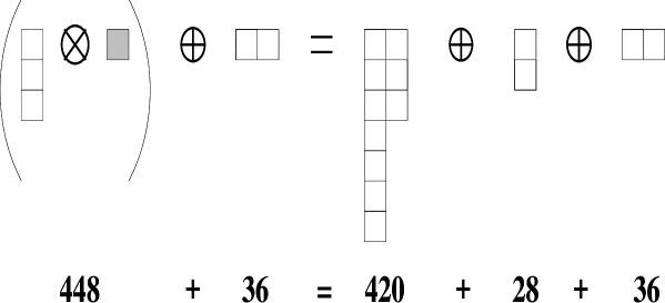
Figure 1: Decomposition in irreducible representations of a tensor of type $T^{A}{}_{BCD}$

A similar argument can be given to interpret the second $T$–identity (45). A tensor of type $Z_{[CD]}^{[ABEF]}$ contains, a priori, $70\times 28$ components and contains the irreducible representations 1512, 420 and 28 (see fig. 2). Using eq.(45) one immediately sees that the representations 1512 and 28 must vanish and that the surviving 420 is proportional through a fixed coefficient to the 420 representations appearing in the decomposition of the $T^{A}{}_{B[CD]}$ tensor.

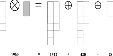
Figure 2: Decomposition in irreducible representations of a tensor of type $Z^{CD}_{ABEF}$

In view of this discussion, the $T$–identities can be rewritten as follows in the basis of the independent irreducible tensors

$${\stackrel{{\scriptstyle\circ}}{{{}^{\phantom{A}}T^{A}}}}{}_{BCD} = T^{A}{}_{[BCD]}$$

$${\stackrel{{\scriptstyle\circ}}{{T}}}_{AB} = T^{M}{}_{AMB}$$ (47)

The irreducible tensors 420 and 36 can be identified, through a suitable coefficient fixed by Bianchi identities, with the fermion shifts appearing in the supersymmetry transformation rules (21):

$$\Sigma^{A}_{BCD}\,=\,\sigma{\stackrel{{\scriptstyle\circ}}{{{}^{\phantom{A}}T^{A}}}}_{BCD}\quad;\quad S_{DB}\,=\,s\,{\stackrel{{\scriptstyle\circ}}{{T}}}_{DB}$$ (48)

2.2.3 The Ward identity and the potential

Finally, according to a general mechanism present in all extended supergravities [10] the scalar potential is defined by the following supersymmetry Ward identity:

$$-{\cal V}\,\delta^{A}_{B}\,=\,S_{AM}\,S^{BM}\,-\,\Sigma_{A}^{PQR}\,\Sigma^{B}_{PQR}$$ (49)

which, as shown by de Wit and Nicolai [17] is satisfied if and only if the ratio between the two constants in eq. (48) is:

$$\frac{s^{2}}{\sigma^{2}}\,=\,\frac{18}{49}$$ (50)

3 Algebraic characterization of the gauge group embedding $G_{gauge}\longrightarrow SL(8,{\rm I\kern-1.79993ptR})$

As we have seen in the previous section the existence of gauged supergravity models relies on a peculiar pair of identities to be satisfied by the $T$–tensors. Therefore a classification of all possible gaugings involves a parametrization of all $SL(8,{\rm I\kern-1.79993ptR})$ subalgebras that lead to satisfied $T$–identities. Since the $T$–tensors are scalar field dependent objects it is not immediately obvious how such a program can be carried through. On the other hand since the problem is algebraic in nature (one looks for all Lie subalgebras of $SL(8,{\rm I\kern-1.79993ptR})$ fulfilling a certain property) it is clear that it should admit a completely algebraic formulation. It turns out that such an algebraic formulation is possible and actually very simple. We will show that the $T$–identities imposed on the $T$–tensors are nothing else but a single algebraic equation imposed on the embedding matrix ${\cal E}$ introduced in eq.(36). This is what we do in the present section.

To begin with we recall a general and obvious constraint to be satisfied by ${\cal E}$ which embeds a subalgebra of the $SL(8,{\rm I\kern-1.79993ptR})$ Lie algebra into its ${\bf 28}$ irreducible representation. As it was already stressed in [22], the vectors should be in the coadjoint representation of the gauge group. Hence under reduction to $G_{gauge}\subset SL(8,{\rm I\kern-1.79993ptR})$ we must obtain the following decomposition of the entire set of the electric vectors:

$${\bf 28}\stackrel{{\scriptstyle G_{gauge}}}{{\rightarrow}}{\bf coadj}{G_{gauge}}\oplus{\cal R}$$ (51)

where ${\cal R}$ denotes the subspace of vectors not entering the adjoint representation of $G_{gauge}$ which is not necessarily a representation of $G_{gauge}$ itself.

Next in order to reduce the field dependent $T$–identities to an algebraic equation on ${\cal E}$ we introduce the following constant tensors:

$$t^{(1)}_{\Omega\Sigma}{}^{\Pi\Gamma}{}_{\Delta\Lambda} \equiv \sum_{\alpha}e^{\alpha}_{\Omega\Sigma}\,q^{\Pi\Gamma}{}_{\Delta\Lambda}(\alpha)\,,\,$$

$$t^{(2)}_{\Omega\Sigma}{}^{\Pi\Gamma\Delta\Lambda} \equiv \sum_{\alpha}e^{\alpha}_{\Omega\Sigma}\,p^{\Pi\Gamma\Delta\Lambda}(\alpha)\,.$$ (52)

In terms of $t^{(1)}$ and $t^{(2)}$ the field dependent $T$-tensor is rewritten as

$$T^{A}{}_{BCD}=(u^{\Omega\Sigma}{}_{CD}+v_{\Omega\Sigma CD})\big{[}\,t^{(1)}_{\Omega\Sigma}{}^{\Pi\Gamma}{}_{\Delta\Lambda}\,(u^{AM}{}_{\Pi\Gamma}\,u^{\Delta\Lambda}{}_{BM}-v^{AM\Phi\Gamma}\,v_{\Delta\Lambda BM})\,\,$$

$$+t^{(2)}_{\Omega\Sigma}{}^{\Pi\Gamma\Delta\Lambda}\,(u^{AM}{}_{\Pi\Gamma}\,v^{\Delta\Lambda}{}_{BM}-v^{AM\Phi\Gamma}\,u_{\Delta\Lambda BM})\,\big{]}\,.$$ (53)

Then we can state our main result as the following

Theorem 3.1

The field dependent $T$-identities are fully equivalent to the following algebraic equation:

$$t^{(1)}_{\Omega\Sigma}{}^{\Pi\Gamma}{}_{\Delta\Lambda}+t^{(1)}_{\Delta\Lambda}{}^{\Pi\Gamma}{}_{\Omega\Sigma}+t^{(2)}_{\Pi\Gamma}{}^{\Delta\Lambda}{}^{\Omega\Sigma} = 0\,,$$

Proof 3.1

-

We have to show that the field dependent $T$-identities (44) and (45) are fully equivalent to the algebraic expression (LABEL:lt-id). So we begin with one direction of the proof

1. Proof that (LABEL:lt-id) implies (44) and (45)

   Summing three times (LABEL:lt-id) with permuted indices, one finds

   $$t^{(2)}_{\Omega\Sigma}{}^{\Pi\Gamma}{}^{\Delta\Lambda}+t^{(2)}_{\Delta\Lambda}{}^{\Pi\Gamma}{}^{\Omega\Sigma}-t^{(2)}_{\Pi\Gamma}{}^{\Delta\Lambda}{}^{\Omega\Sigma}=0\,.$$ (55)

   ¿From eq.s (LABEL:lt-id), (55) one finds that

   $$(u^{AB}{}_{\Omega\Sigma}+v^{AB\Omega\Sigma})e_{\Omega\Sigma}^{\alpha}{\cal B}_{CDEF}={2\over 3}\delta^{[A}{}_{[B}T^{C]}{}_{D]GH}+{2\over 3}\delta^{[A}{}_{[G}T^{C]}{}_{H]BD}$$ (56)

   Since ${\cal B}_{CDEF}$ is antisymmetric in $CDEF$, one has

   $$(u^{AB}{}_{\Omega\Sigma}+v^{AB\Omega\Sigma})e_{\Omega\Sigma}^{\alpha}{\cal B}_{CDEF} = \frac{4}{3}\delta^{[A}{}_{[B}T^{C]}{}_{DGH]}\,,$$

   $${2\over 3}\delta^{[A}{}_{[B}T^{C]}{}_{D]GH}+{2\over 3}\delta^{[A}{}_{[G}T^{C]}{}_{H]BD} = \frac{4}{3}\delta^{[A}{}_{[B}T^{C]}{}_{DGH]}\,.$$ (57)

   The first of the above equations coincides with eq. (45). From the second one, taking suitable contractions, as explained in [17], one obtains eq. (44). This shows that (LABEL:lt-id) implies both eq.s (44) and (45).

2. Proof that (44) and (45) imply (LABEL:lt-id)

   If we use (44) to rewrite the following expression

   $${2\over 3}\delta^{[A}{}_{[B}T^{C]}{}_{D]GH}+{2\over 3}\delta^{[A}{}_{[G}T^{C]}{}_{H]BD}=$$

   $$=\left[{2\over 3}\delta^{[A}{}_{[B}T^{C]}{}_{D]GH}\right]_{\left[DGH\right]}+\left[{2\over 3}\delta^{[A}{}_{[G}T^{C]}{}_{H]BD}\right]_{\left[HBD\right]}+$$

   $$+\left[{4\over 21}\delta^{[A}{}_{[B}\delta^{[C}{}_{|G}T^{M}{}_{HM|D]}\right]_{\left[GH\right]}+\left[{4\over 21}\delta^{[A}{}_{[G}\delta^{[C}{}_{|B}T^{M}{}_{DM|H]}\right]_{\left[BD\right]}$$ (58)

   we can easily verify that it is antisymmetric in the indices $GDBH$. Indeed the last two terms cancel, while the sign in front of the first two terms is reversed upon interchanging $B$ and $G$. This means that

   $${2\over 3}\delta^{[A}{}_{[B}T^{C]}{}_{D]GH}+{2\over 3}\delta^{[A}{}_{[G}T^{C]}{}_{H]BD}=\frac{4}{3}\delta^{[A}{}_{[B}T^{C]}{}_{DGH]}$$ (59)

   So, because of equation (45), we have:

   $${2\over 3}\delta^{[A}{}_{[B}T^{C]}{}_{D]GH}+{2\over 3}\delta^{[A}{}_{[G}T^{C]}{}_{H]BD}=(u^{AB}{}_{\Omega\Sigma}+v^{AB\Omega\Sigma})e_{\Omega\Sigma}^{\alpha}{\cal B}_{CDEF}$$ (60)

   By inserting the expressions of $T$ and $\cal B$ in terms of the $t$’s into equation (60) and collecting the coefficients the independent scalar–field components, we retrieve equation (LABEL:lt-id).

   This concludes our proof.

4 Solution of the algebraic $t$–identity

The algebraic $t$–identity (LABEL:lt-id) is a linear equation imposed on the embedding matrix ${\cal E}$. We have solved it by means of a computer program and we have found the 36–parameter solution displayed in tables 3, 4,5, 6,7,8,9,10, 11. In order to explain the content of these tables we have to describe our notations and our construction in more detail.

4.1 Embedding of the electric group

The first information we need to specify is the explicit embedding of the electric subalgebra $SL(8,{\rm I\kern-1.79993ptR})$ into the U–duality algebra $E_{7(7)}$. For this latter we adopt the conventions and notations of [8].

4.1.1 The $E_{7(7)}$ algebra: roots and weights

We consider the standard $E_{7}$ Dynkin diagram (see fig. $3$) and we name $\alpha_{i}$ ($i=1,\dots,7$) the corresponding simple roots.

Figure 3: $E_{7}$ Dynkin diagram and root labeling

Having fixed this basis, each $E_{7(7)}$ root is intrinsically identified by its Dynkin labels, namely by its integer valued components in the simple root basis.

Having identified the roots, the next step we need is the construction of the real fundamental representation $SpD(56)$ of our U–duality Lie algebra $E_{7(7)}$. For this we need the corresponding weight vectors ${\vec{W}}$.

A particularly relevant property of the maximally non–compact real sections of a simple complex Lie algebra is that all its irreducible representations are real. $E_{7(7)}$ is the maximally non compact real section of the complex Lie algebra $E_{7}$, hence all its irreducible representations $\Gamma$ are real. This implies that if an element of the weight lattice ${\vec{W}}\,\in\,\Lambda_{w}$ is a weight of a given irreducible representation ${\vec{W}}\in\Gamma$ then also its negative is a weight of the same representation: $-{\vec{W}}\in\Gamma$. Indeed changing sign to the weights corresponds to complex conjugation.

According to standard Lie algebra lore every irreducible representation of a simple Lie algebra  $\vrule height=6.45831pt,width=0.4pt,depth=0.0pt\kern-3.00003pt{\rm G}$ is identified by a unique highest weight ${\vec{W}}_{max}$. Furthermore all weights can be expressed as integral non–negative linear combinations of the simple weights ${\vec{W}}_{\ell}\,(\ell=1,...,r=\mbox{rank}(\,\hbox{$\vrule height=6.45831pt,width=0.4pt,depth=0.0pt\kern-3.00003pt{\rm G}$}))$, whose components are named the Dynkin labels of the weight. The simple weights ${\vec{W}}_{i}$ of  $\vrule height=6.45831pt,width=0.4pt,depth=0.0pt\kern-3.00003pt{\rm G}$ are the generators of the dual lattice to the root lattice and are defined by the condition:

$$\frac{2({\vec{W}}_{i}\,,\,{\vec{\alpha}}_{j})}{({\vec{\alpha}}_{j}\,,\,{\vec{\alpha}}_{j})}=\delta_{ij}$$ (61)

In the simply laced $E_{7(7)}$ case, the previous equation simplifies as follows

$$({\vec{W}}_{i}\,,\,{\vec{\alpha}}_{j})=\delta_{ij}$$ (62)

where ${\vec{\alpha}}_{j}$ are the the simple roots. Using the Dynkin diagram of $E_{7(7)}$ (see fig. $3$) from eq.(62) we can easily obtain the explicit expression of the simple weights.

The Dynkin labels of the highest weight of an irreducible representation $\Gamma$ give the Dynkin labels of the representation. Therefore the representation is usually denoted by $\Gamma[n_{1},...,n_{r}]$. All the weights ${\vec{W}}$ belonging to the representation $\Gamma$ can be described by $r$ integer non–negative numbers $q^{\ell}$ defined by the following equation:

$${\vec{W}}_{max}-{\vec{W}}=\sum_{\ell=1}^{r}q^{\ell}{\vec{\alpha}}_{\ell}$$ (63)

where $\alpha_{\ell}$ are the simple roots. According to this standard formalism the fundamental real representation $SpD(56)$ of $E_{7(7)}$ is $\Gamma[1,0,0,0,0,0,0]$ and the expression of its weights in terms of $q^{\ell}$ is given in table 1, the highest weight being ${\vec{W}}^{(51)}$.

We can now explain the specific ordering of the weights we have adopted.

First of all we have separated the $56$ weights in two groups of $28$ elements so that the first group:

$${\vec{\Lambda}}^{(n)}={\vec{W}}^{(n)}\quad n=1,...,28$$ (64)

are the weights for the irreducible 28 dimensional representation of the electric subgroup $SL(8,{\rm I\kern-1.79993ptR})\subset E_{7(7)}$. The remaining group of $28$ weight vectors are the weights for the transposed representation of the same group that we name ${\bf\overline{28}}$.

Secondly the $28$ weights ${\vec{\Lambda}}$ have been arranged according to the decomposition with respect to the T–duality subalgebra $SO(6,6)\subset E_{7}(7)$: the first $16$ correspond to R–R vectors and are the weights of the spinor representation of $SO(6,6)$ while the last $12$ are associated with N–S fields and correspond to the weights of the vector representation of $SO(6,6)$.

4.1.2 The matrices of the fundamental 56 representation

Equipped with the weight vectors we can now proceed to the explicit construction of the ${\bf SpD(56)}$ representation of $E_{7(7)}$. In our construction the basis vectors are the $56$ weights, according to the enumeration of table 1. What we need are the $56\times 56$ matrices associated with the $7$ Cartan generators $H_{{\vec{\alpha}}_{i}}$ ($i=1,\dots,7$) and with the $126$ step operators $E^{\vec{\alpha}}$ that are defined by:

$$\left[SpD_{56}\left(H_{{\vec{\alpha}}_{i}}\right)\right]_{nm} \equiv \langle{\vec{W}}^{(n)}|\,H_{{\vec{\alpha}}_{i}}\,|{\vec{W}}^{(m)}\rangle$$

$$\left[SpD_{56}\left(E^{{\vec{\alpha}}}\right)\right]_{nm} \equiv \langle{\vec{W}}^{(n)}|\,E^{{\vec{\alpha}}}\,|{\vec{W}}^{(m)}\rangle$$ (65)

Let us begin with the Cartan generators. As a basis of the Cartan subalgebra we use the generators $H_{\vec{\alpha}_{i}}$ defined by the commutators:

$$\left[E^{{\vec{\alpha}}_{i}},E^{-{\vec{\alpha}}_{i}}\right]\,\equiv\,H_{\vec{\alpha}_{i}}$$ (66)

In the $SpD(56)$ representation the corresponding matrices are diagonal and of the form:

$$\langle{\vec{W}}^{(p)}|\,H_{\vec{\alpha}_{i}}\,|{\vec{W}}^{(q)}\rangle\,=\,\left({\vec{W}}^{(p)},{\vec{\alpha}_{i}}\right)\delta_{p\,q}\quad;\quad(p,q\,=\,1,...,56)$$ (67)

The scalar products

$$\left({\vec{\Lambda}}^{(n)}\,\cdot\,{\vec{h}},-{\vec{\Lambda}}^{(m)}\,\cdot\,{\vec{h}}\right)\,=\,\left({\vec{W}}^{(p)}\,\cdot\,{\vec{h}}\right)\quad;\quad(n,m=1,...,28\,;\,p=1,...,56)$$ (68)

are to be understood in the following way:

$${\vec{W}}^{(p)}\,\cdot\,{\vec{h}}\,=\,\sum_{i=1}^{7}\left({\vec{W}}^{(p)},{\vec{\alpha}_{i}}\right)h^{i}$$ (69)

Next we construct the matrices associated with the step operators. Here the first observation is that it suffices to consider the positive roots. Because of the reality of the representation, the matrix associated with the negative of a root is just the transposed of that associated with the root itself:

$$E^{-\alpha}=\left[E^{\alpha}\right]^{T}\,\leftrightarrow\,\langle{\vec{W}}^{(n)}|\,E^{-{\vec{\alpha}}}\,|{\vec{W}}^{(m)}\rangle\,=\,\langle{\vec{W}}^{(m)}|\,E^{{\vec{\alpha}}}\,|{\vec{W}}^{(n)}\rangle$$ (70)

The method we have followed to obtain the matrices for all the positive roots is that of constructing first the $56\times 56$ matrices for the step operators $E^{\vec{\alpha}_{\ell}}\,(\ell=1,...,7)$ associated with the simple roots and then generating all the others through their commutators. The construction rules for the $SpD(56)$ representation of the six operators $E^{\alpha_{\ell}}\,(\ell\neq 5)$ are:

$$\ell\,\neq\,5\quad\,\Biggl{\{}\matrix{\langle{\vec{W}}^{(n)}|\,E^{\vec{\alpha}_{\ell}}\,|{\vec{W}}^{(m)}\rangle&=&\delta_{{\vec{W}}^{(n)},{\vec{W}}^{(m)}+{\vec{\alpha}}_{\ell}}&;&n,m=1,\dots,28\cr\langle{\vec{W}}^{(n+28)}|\,E^{\vec{\alpha}_{\ell}}\,|{\vec{W}}^{(m+28)}\rangle&=&-\delta_{{\vec{W}}^{(n+28)},{\vec{W}}^{(m+28)}+{\vec{\alpha}}_{\ell}}&;&n,m=1,\dots,28\cr}$$ (71)

The six simple roots ${\vec{\alpha}_{\ell}}$ with $\ell\neq 5$ belong also to the the Dynkin diagram of the electric subgroup SL(8,IR). Thus their shift operators have a block diagonal action on the 28 and ${\bf\overline{28}}$ subspaces of the $SpD(56)$ representation that are irreducible under the electric subgroup. From eq.(71) we conclude that:

$$\ell\,\neq\,5\quad\,SpD_{56}\left(E^{{\vec{\alpha}}_{\ell}}\right)=\left(\matrix{A[{{\vec{\alpha}}_{\ell}}]&{\bf 0}\cr{\bf 0}&-A^{T}[{{\vec{\alpha}}_{\ell}}]\cr}\right)$$ (72)

the $28\times 28$ block $A[{{\vec{\alpha}}_{\ell}}]$ being defined by the first line of eq.(71).

On the contrary the operator $E^{\vec{\alpha}_{5}}$, corresponding to the only root of the $E_{7}$ Dynkin diagram that is not also part of the $A_{7}$ diagram is represented by a matrix whose non–vanishing $28\times 28$ blocks are off–diagonal. We have

$$SpD_{56}\left(E^{{\vec{\alpha}}_{5}}\right)=\left(\matrix{{\bf 0}&B[{{\vec{\alpha}}_{5}}]\cr C[{{\vec{\alpha}}_{5}}]&{\bf 0}\cr}\right)$$ (73)

where both $B[{{\vec{\alpha}}_{5}}]=B^{T}[{{\vec{\alpha}}_{5}}]$ and $C[{{\vec{\alpha}}_{5}}]=C^{T}[{{\vec{\alpha}}_{5}}]$ are symmetric $28\times 28$ matrices. More explicitly the matrix $SpD_{56}\left(E^{{\vec{\alpha}}_{5}}\right)$ is given by:

$$\langle{\vec{W}}^{(n)}|\,E^{\vec{\alpha}_{5}}\,|{\vec{W}}^{(m+28)}\rangle\,=\,\langle{\vec{W}}^{(m)}|\,E^{\vec{\alpha}_{5}}\,|{\vec{W}}^{(n+28)}\rangle$$

$$\langle{\vec{W}}^{(n+28)}|\,E^{\vec{\alpha}_{5}}\,|{\vec{W}}^{(m)}\rangle\,=\,\langle{\vec{W}}^{(m+28)}|\,E^{\vec{\alpha}_{5}}\,|{\vec{W}}^{(n)}\rangle$$ (74)

with

$$\begin{array}[]{rcrcrcrcrcr}\langle{\vec{W}}^{(7)}|\,E^{\vec{\alpha}_{5}}\,|{\vec{W}}^{(44)}\rangle&=&-1&\hbox{}\hfil&\langle{\vec{W}}^{(8)}|\,E^{\vec{\alpha}_{5}}\,|{\vec{W}}^{(42)}\rangle&=&1&\hbox{}\hfil&\langle{\vec{W}}^{(9)}|\,E^{\vec{\alpha}_{5}}\,|{\vec{W}}^{(43)}\rangle&=&-1\\ \langle{\vec{W}}^{(14)}|\,E^{\vec{\alpha}_{5}}\,|{\vec{W}}^{(36)}\rangle&=&1&\hbox{}\hfil&\langle{\vec{W}}^{(15)}|\,E^{\vec{\alpha}_{5}}\,|{\vec{W}}^{(37)}\rangle&=&-1&\hbox{}\hfil&\langle{\vec{W}}^{(16)}|\,E^{\vec{\alpha}_{5}}\,|{\vec{W}}^{(35)}\rangle&=&-1\\ \langle{\vec{W}}^{(29)}|\,E^{\vec{\alpha}_{5}}\,|{\vec{W}}^{(6)}\rangle&=&-1&\hbox{}\hfil&\langle{\vec{W}}^{(34)}|\,E^{\vec{\alpha}_{5}}\,|{\vec{W}}^{(1)}\rangle&=&-1&\hbox{}\hfil&\langle{\vec{W}}^{(49)}|\,E^{\vec{\alpha}_{5}}\,|{\vec{W}}^{(28)}\rangle&=&1\\ \langle{\vec{W}}^{(50)}|\,E^{\vec{\alpha}_{5}}\,|{\vec{W}}^{(27)}\rangle&=&-1&\hbox{}\hfil&\langle{\vec{W}}^{(55)}|\,E^{\vec{\alpha}_{5}}\,|{\vec{W}}^{(22)}\rangle&=&-1&\hbox{}\hfil&\langle{\vec{W}}^{(56)}|\,E^{\vec{\alpha}_{5}}\,|{\vec{W}}^{(21)}\rangle&=&1\\ \end{array}$$ (75)

In this way we have completed the construction of the $E^{{\vec{\alpha}}_{\ell}}$ operators associated with simple roots. For the matrices associated with higher roots we just proceed iteratively in the following way. As usual we organize the roots by height :

$${\vec{\alpha}}=n^{\ell}\,{\vec{\alpha}}_{\ell}\quad\rightarrow\quad\mbox{ht}\,{\vec{\alpha}}\,=\,\sum_{\ell=1}^{7}n^{\ell}$$ (76)

and for the roots $\alpha_{i}+\alpha_{j}$ of height $\mbox{ht}=2$ we set:

$$SpD_{56}\left(E^{\alpha_{i}+\alpha_{j}}\right)\equiv\left[SpD_{56}\left(E^{\alpha_{i}}\right)\,,\,SpD_{56}\left(E^{\alpha_{i}}\right)\right]\quad;\quad i<j$$ (77)

Next for the roots of $\mbox{ht}=3$ that can be written as $\alpha_{i}+\beta$ where $\alpha_{i}$ is simple and $\mbox{ht}\,\beta\,=\,2$ we write:

$$SpD_{56}\left(E^{\alpha_{i}+\beta}\right)\equiv\left[SpD_{56}\left(E^{\alpha_{i}}\right)\,,\,SpD_{56}\left(E^{\beta}\right)\right]$$ (78)

Obtained the matrices for the roots of $\mbox{ht}=3$ one proceeds in a similar way for those of the next height and so on up to exhaustion of all the $63$ positive roots.

This concludes our description of the algorithm by means of which our computer program constructed all the $133$ matrices spanning the $E_{7(7)}$ Lie algebra in the $SpD(56)$ representation. A fortiori, if we specify the embedding we have the matrices generating the electric subgroup $SL(8,{\rm I\kern-1.79993ptR})$.

4.1.3 The $SL(8,{\rm I\kern-1.79993ptR})$ subalgebra

The Electric $Sl(8,{\rm I\kern-1.79993ptR})$ subalgebra is identified in $E_{7(7)}$ by specifying its simple roots $\beta_{i}$ spanning the standard $A_{7}$ Dynkin diagram. The Cartan generators are the same for the $E_{7(7)}$ Lie algebra as for the $SL(8,{\rm I\kern-1.79993ptR})$ subalgebra and if we give $\beta_{i}$ every other generator is defined. The basis we have chosen is the following one:

$$\begin{array}[]{ccccccc}\beta_{1}&=&\,\alpha_{2}+2\alpha_{3}+3\alpha_{4}+2\alpha_{5}+2\alpha_{6}+\alpha_{7}&;&\beta_{2}&=&\alpha_{1}\cr\beta_{3}&=&\,\alpha_{2}&;&\beta_{4}&=&\alpha_{3}\cr\beta_{5}&=&\,\alpha_{4}&;&\beta_{6}&=&\alpha_{6}\cr\beta_{7}&=&\,\alpha_{7}&\hbox{}\hfil&\hbox{}\hfil&\hbox{}\hfil&\hbox{}\hfil\cr\end{array}$$ (79)

The complete set of positive roots of $SL(8{\rm I\kern-1.79993ptR})$ is then composed of $28$ elements that we name $\rho_{i}$ ($i=1,\dots,28$) and that are enumerated according to our chosen order in table 2.

Table 2: The choice of the order of the $SL(8,{\rm I\kern-1.79993ptR})$ roots:

$\rho_{1}\,\equiv\,$	$\beta_{2}$
$\rho_{2}\,\equiv\,$	$\beta_{2}+\beta_{3}$
$\rho_{3}\,\equiv\,$	$\beta_{2}+\beta_{3}+\beta_{4}$
$\rho_{4}\,\equiv\,$	$\beta_{2}+\beta_{3}+\beta_{4}+\beta_{5}$
$\rho_{5}\,\equiv\,$	$\beta_{2}+\beta_{3}+\beta_{4}+\beta_{5}+\beta_{6}$
$\rho_{6}\,\equiv\,$	$\beta_{3}$
$\rho_{7}\,\equiv\,$	$\beta_{3}+\beta_{4}$
$\rho_{8}\,\equiv\,$	$\beta_{3}+\beta_{4}+\beta_{5}$
$\rho_{9}\,\equiv\,$	$\beta_{3}+\beta_{4}+\beta_{5}+\beta_{6}$
$\rho_{10}\,\equiv\,$	$\beta_{4}$
$\rho_{11}\,\equiv\,$	$\beta_{4}+\beta_{5}$
$\rho_{12}\,\equiv\,$	$\beta_{4}+\beta_{5}+\beta_{6}$
$\rho_{13}\,\equiv\,$	$\beta_{5}$
$\rho_{14}\,\equiv\,$	$\beta_{5}+\beta_{6}$
$\rho_{15}\,\equiv\,$	$\beta_{6}$
$\rho_{16}\,\equiv\,$	$\beta_{1}+\beta_{2}+\beta_{3}+\beta_{4}+\beta_{5}+\beta_{6}+\beta_{7}$
$\rho_{17}\,\equiv\,$	$\beta_{2}+\beta_{3}+\beta_{4}+\beta_{5}+\beta_{6}+\beta_{7}$
$\rho_{18}\,\equiv\,$	$\beta_{3}+\beta_{4}+\beta_{5}+\beta_{6}+\beta_{7}$
$\rho_{19}\,\equiv\,$	$\beta_{4}+\beta_{5}+\beta_{6}+\beta_{7}$
$\rho_{20}\,\equiv\,$	$\beta_{5}+\beta_{6}+\beta_{7}$
$\rho_{21}\,\equiv\,$	$\beta_{6}+\beta_{7}$
$\rho_{22}\,\equiv\,$	$\beta_{1}$
$\rho_{23}\,\equiv\,$	$\beta_{1}+\beta_{2}$
$\rho_{24}\,\equiv\,$	$\beta_{1}+\beta_{2}+\beta_{3}$
$\rho_{25}\,\equiv\,$	$\beta_{1}+\beta_{2}+\beta_{3}+\beta_{4}$
$\rho_{26}\,\equiv\,$	$\beta_{1}+\beta_{2}+\beta_{3}+\beta_{4}+\beta_{5}$
$\rho_{27}\,\equiv\,$	$\beta_{1}+\beta_{2}+\beta_{3}+\beta_{4}+\beta_{5}+\beta_{6}$
$\rho_{28}\,\equiv\,$	$\beta_{7}$

Hence the $63$ generators of the $SL(8,{\rm I\kern-1.79993ptR})$ Lie algebra are:

$$\begin{array}[]{ccc}\mbox{The 7 Cartan generators}&C_{i}=H_{\alpha_{i}}&i=1,\dots,7\cr\mbox{The 28 positive root generators}&E^{\rho_{i}}&i=1,\dots,28\cr\mbox{The 28 negative root generators}&E^{-\rho_{i}}&i=1,\dots,28\cr\end{array}$$ (80)

and since the $56\times 56$ matrix representation of each $E_{7(7)}$ Cartan generator or step operator was constructed in the previous subsection it is obvious that it is in particular given for the subset of those that belong to the $SL(8,{\rm I\kern-1.79993ptR})$ subalgebra. The basis of this matrix representation is provided by the weights enumerated in table 1.

In this way we have concluded our illustration of the basis in which we have solved the algebraic $t$–identity. The result is the $28\times 63$ matrix:

$${\cal E}(h,\ell)\,\longrightarrow\,e^{\alpha}_{W}(h,\ell)$$ (81)

where the index $W$ runs on the $28$ negative weights of table 1, while the index $\alpha$ runs on all the $SL(8,{\rm I\kern-1.79993ptR})$ generators according to eq. (80). The matrix ${\cal E}(h,p)$ depends on $36$ parameters that we have named:

$$\begin{array}[]{cc}h_{i}&i=1,\dots,8\cr\ell_{i}&i=1,\dots,28\cr\end{array}$$ (82)

and its entries are explicitly displayed in tables 3, 4,5, 6,7,8,9,10, 11 as we have already stressed at the beginning of this section. The distinction between the $h_{i}$ parameters and the $\ell_{i}$ parameters has been drawn in the following way:

• The $8$ parameters $h_{i}$ are those that never multiply a Cartan generator

• The $28$ parameters $\ell_{i}$ are those that multiply at least one Cartan generator.

In other words if we set all the $\ell_{i}=0$ the gauge subalgebra $G_{gauge}\subset SL(8,{\rm I\kern-1.79993ptR})$ is composed solely of step operators while if you switch on also the $\ell_{i}$.s then some Cartan generators appear in the Lie algebra. This distinction will be very useful in classifying the independent solutions.

5 Classification of gauged $N=8$ supergravities

Equipped with the explicit solution of the $t$–identity encoded in the embedding matrix ${\cal E}$ we can now address the complete classification of the gauged supergravity models. As already anticipated in the introduction our result is that the complete set of possible theories coincides with the gaugings found by Hull [24] (together with the ones simply outlined by Hull [24]) in the middle of the eighties and correspond to all possible non–compact real forms of the $SO(8)$ Lie algebra plus a number of Inonu–Wigner contractions thereof. Since Hull’s method to obtain these gaugings was not based on an exhaustive analysis the doubt existed whether his set of theories was complete or not. Our analysis shows that in fact it was. Furthermore since our method is constructive it provides the means to study in a systematic way the features of all these models. In this section we derive such a result.

We have to begin our discussion with two observations:

1. The solution of $t$–identities encoded in the matrix ${\cal E}(h,\ell)$ is certainly overcomplete since we are still free to conjugate any gauge algebra $G_{gauge}$ with an arbitrary finite element of the electric group $g\,\in\,SL(8,{\rm I\kern-1.79993ptR})$: $G^{\prime}_{gauge}=g\,G_{gauge}\,g^{-1}$ yields a completely physically equivalent gauging as $G_{gauge}$. This means that we need to consider the $SL(8,{\rm I\kern-1.79993ptR})$ transformations of the matrix ${\cal E}(h,\ell)$ defined as:

   $$\forall\,g\,\in\,SL(8,{\rm I\kern-1.79993ptR})\,:\,g\cdot{\cal E}(h,\ell)\equiv D_{28}(g^{-1})\,{\cal E}(h,\ell)\,D_{63}(g)$$ (83)

   where $D_{28}(g)$ and $D_{63}(g)$ denote the matrices of the ${\bf 28}$ and the ${\bf 63}$ representation respectively. If two set of parameters $\{h,\ell\}$ and $\{h^{\prime},\ell^{\prime}\}$ are related by an $SL(8,{\rm I\kern-1.79993ptR})$ conjugation, in the sense that:

   $$\exists g\,\in\,SL(8,{\rm I\kern-1.79993ptR})\,:\,{\cal E}(h^{\prime},\ell^{\prime})=g\cdot{\cal E}(h,\ell)$$ (84)

   then the theories described by $\{h,\ell\}$ and $\{h^{\prime},\ell^{\prime}\}$ are the same theory. In other words what we need is the space of orbits of $SL(8,{\rm I\kern-1.79993ptR})$ inequivalent embedding matrices.

2. Possible theories obtained by choosing a set of $\{h,\ell\}$ parameters are further restricted by the constraints that

   • The selected generators of $SL(8,{\rm I\kern-1.79993ptR})$ should close a Lie subalgebra $G_{gauge}$

   • The selected vectors (=weights, see table 1) should transform in the coadjoint representation $Coadj\left(G_{gauge}\right)$

In view of these observations a natural question we should pose is the following one: is there a natural way to understand why the number of parameters on which the embedding matrix depends is, a part from an immaterial overall constant, precisely 35?. The answer is immediate and inspiring. Because of point 2) in the above list of properties the $28$ linear combinations of $SL(8,{\rm I\kern-1.79993ptR})$ generators:

$$T_{W}\equiv e_{W}^{\phantom{W}\alpha}\left(h,\ell\right)\,G_{\alpha}$$ (85)

must span the adjoint representation of a $28$–dimensional subalgebra $G_{gauge}(h,\ell)$ of the $SL(8,{\rm I\kern-1.79993ptR})$ algebra.

Naming ${\cal G}_{gauge}(h,\ell)$ the corresponding Lie subgroup, because of its very definition we have that the matrix ${\cal E}(h,\ell)$ is invariant under transformations of ${\cal G}_{gauge}(h,\ell)$ :

$$\forall\,\gamma\,\in\,{\cal G}_{gauge}(h,\ell\,\subset\,SL(8,{\rm I\kern-1.79993ptR}):\quad\gamma\,\cdot\,{\cal E}(h,\ell)={\cal E}(h,\ell)$$ (86)

Comparing eq.(86) with eq.(83) we see that having fixed a matrix ${\cal E}(h,\ell)$ and hence an algebra ${\cal G}_{gauge}(h,\ell)$, according to point 1) of the above discussion we can obtain a $35$–dimensional orbit of equivalent embedding matrices:

$${\cal E}\left(h^{\prime}(\mu),\ell^{\prime}(\mu)\right)\,\equiv\,g(\mu)\,\cdot\,{\cal E}(h,\ell)\quad\mbox{where}\quad g(\mu)\,\in\,\frac{SL(8,{\rm I\kern-1.79993ptR})}{{\cal G}_{gauge}(h,\ell)}$$ (87)

Hence, $35=63-28$ is the dimension of the coset manifold ${SL(8,{\rm I\kern-1.79993ptR})}/{{\cal G}_{gauge}(h,\ell)}$ and ${\cal E}\left(h^{\prime}(\mu),\ell^{\prime}(\mu)\right)$ is the embedding matrix for the family of conjugated, isomorphic, Lie algebras:

$${\cal G}_{gauge}\left(h^{\prime}(\mu),\ell^{\prime}(\mu)\right)\,=g^{-1}(\mu)\,{{\cal G}_{gauge}(h,\ell)}\,g(\mu)$$ (88)

An essential and a priori unexpected conclusion follows from this discussion.

Proposition 5.1

The gauged $N=8$ supergravity models cannot depend on more than a single continuous parameter (=coupling constant), even if they correspond to gauging a multidimensional abelian algebra

Proof 5.1

-

Since the explicit solution of the algebraic $t$–identities has produced an embedding matrix ${\cal E}(h,\ell)$ depending on no more than $36$–parameters, then the only continuous parameter which is physically relevant is the overall proportionality constant. The remaining $35$–parameters can be reabsorbed by $SL(8,{\rm I\kern-1.61993ptR})$ conjugations according to eq.(88)

In other words what we have found is that the space of orbits we are looking for is a discrete space. The classifications of gauged supergravity models is just a classification of gauge algebras a single coupling constant being assigned to each case. This is considerably different from other supergravities with less supersymmetries, like the $N=2$ case. There gauging a group $G_{gauge}$ involves as many coupling constants as there are simple factors in $G_{gauge}$. So in those cases not only we have a much wider variety of possible gauge algebras but also we have lagrangians depending on several continuous parameters. In the $N=8$ case supersymmetry constraints the theory in a much stronger way. We want to stress that this is an yield of supersymmetry and not of Lie algebra theory. It is the algebraic $t$–identity, enforced by the closure of Bianchi identities, that admits a general solution depending only on $36$–parameters. If the solution depended on $35+m$ parameters then we might have introduced $m$ relevant continuous parameters into the Lagrangian.

Relying on these observations we are left with the problem of classifying the orbit space already knowing that it is composed of finite number of discrete elements. Orbits are characterized in terms of invariants, so we have to ask ourselves what is the natural invariant associated with the embedding matrix ${\cal E}(h,\ell)$. The answer is once again very simple. It is the signature of the Killing–Cartan 2–form for the resulting gauge algebra ${\cal G}_{gauge}(h,\ell)$. Consider the $28$ generators (85) and define:

$$\begin{array}[]{rcl}\eta_{W_{1}W_{2}}\left(h,\ell\right)&\equiv&\mbox{Tr}\,\left(T_{W_{1}}\,T_{W_{1}}\right)\cr\hbox{}\hfil&=&e_{W_{1}}^{\phantom{W_{1}}\alpha}\left(h,\ell\right)\,e_{W_{2}}^{\phantom{W_{1}}\beta}\left(h,\ell\right)\,\mbox{Tr}\,\left(G_{\alpha}\,G_{\beta}\right)\cr\hbox{}\hfil&=&e_{W_{1}}^{\phantom{W_{1}}\alpha}\left(h,\ell\right)\,e_{W_{2}}^{\phantom{W_{1}}\beta}\left(h,\ell\right)\,B_{\alpha\beta}\cr\end{array}$$ (89)

where the trace $Tr$ is taken over any representation and the constant matrix $B_{\alpha\beta}\equiv\mbox{Tr}\,\left(G_{\alpha}\,G_{\beta}\right)$ is the Killing–Cartan 2–form of the $SL(2,{\rm I\kern-1.79993ptR})$ Lie algebra. The $28\times 28$ matrix is the Killing–Cartan 2–form of the gauge algebra $G_{gauge}$. As it is well known from general Lie algebra theory, by means of suitable changes of bases inside the same Lie algebra the matrix $\eta_{W_{1}W_{2}}\left(h,\ell\right)$ can be diagonalized and its eigenvalues can be reduced to be either of modulus one or zero. What cannot be done since it corresponds to an intrinsic characterization of the Lie algebra is to change the signature of $\eta_{W_{1}W_{2}}\left(h,\ell\right)$, namely the ordered set of $28$ signs (or zeros) appearing on the principal diagonal when $\eta_{W_{1}W_{2}}\left(h,\ell\right)$ is reduced to diagonal form. Hence what is constant throughout an $SL(8,{\rm I\kern-1.79993ptR})$ orbit is the signature. Let us name $\Sigma\left(\mbox{orbit}\right)$ the $28$ dimensional vector characterizing the signature of an orbit:

$$\Sigma\left(\mbox{orbit}\right)\,\equiv\,\mbox{signature}\,\left[\eta_{W_{1}W_{2}}\left(h^{\prime}(\mu),\ell^{\prime}(\mu)\right)\,\right]$$ (90)

¿From our discussion we conclude that

Proposition 5.2

The classification of gauged N=8 models has been reduced to the classification of the signature vectors $\Sigma\left(\mbox{orbit}\right)$ of eq.(90)

The procedure to calculate $\Sigma\left(\mbox{orbit}\right)$ associated with an orbit $\eta_{W_{1}W_{2}}\left(h^{\prime}(\mu),\ell^{\prime}(\mu)\right)\,$ is that of choosing the representative $\left(h^{\prime}(\mu_{0}),\ell^{\prime}(\mu_{0})\right)$ for which the corresponding matrix $\eta_{W_{1}W_{2}}\bigl{(}h^{\prime}(\mu_{0}),$ $\ell^{\prime}(\mu_{0})\bigr{)}\,$ is diagonal and then to evaluate the signs of the diagonal elements. In principle finding the appropriate $h^{\prime}(\mu_{0}),\ell^{\prime}(\mu_{0})$ could be a difficult task since we are supposed to diagonalize a $28\times 28$ matrix. However our choice of coordinates on the parameter space is such that our task becomes very simple. Using the results of tables 3, 4,5, 6,7,8,9,10, 11 we can calculate the matrix $\eta_{W_{1}W_{2}}\left(h,\ell\right)\,$ and for generic values of $h_{i}$ and $\ell_{i}$ we find that all of its $28\times 28$ entries are non vanishing; yet setting $\ell_{i}=0$ the matrix becomes automatically diagonal and we get:

$$\begin{array}[]{rlcccccccl}\eta\left(h,\ell=0\right)\,=&\mbox{diag}\Bigl{\{}&-{h_{7}}\,{h_{8}},&{h_{1}}\,{h_{6}},&{h_{2}}\,{h_{6}},&-{h_{3}}\,{h_{6}}&,{h_{4}}\,{h_{6}},&-{h_{5}}\,{h_{6}},&{h_{1}}\,{h_{2}},&\hbox{}\cr\hbox{}\hfil&\hbox{}&-{h_{1}}\,{h_{3}},&{h_{1}}\,{h_{4}},&-{h_{1}}\,{h_{5}},&-{h_{2}}\,{h_{5}},&{h_{3}}\,{h_{5}},&-{h_{4}}\,{h_{5}},&{h_{2}}\,{h_{4}},&\hbox{}\cr\hbox{}\hfil&\hbox{}&-{h_{2}}\,{h_{3}},&-{h_{3}}\,{h_{4}},&{h_{1}}\,{h_{7}},&{h_{2}}\,{h_{7}},&-{h_{3}}\,{h_{7}},&{h_{4}}\,{h_{7}},&-{h_{5}}\,{h_{7}},&\hbox{}\cr\hbox{}\hfil&\hbox{}&{h_{6}}\,{h_{7}},&-{h_{1}}\,{h_{8}},&-{h_{2}}\,{h_{8}},&{h_{3}}\,{h_{8}},&-{h_{4}}\,{h_{8}},&{h_{5}}\,{h_{8}},&-{h_{6}}\,{h_{8}}&\Bigr{\}}\cr\end{array}$$ (91)

Hence all possible signatures $\Sigma\left(orbit\right)$ are obtained by assigning to the parameters $h_{i}$ the values $1,-1,0$ in all possible ways. Given an $h$ vector constructed in this way we have then to check that the corresponding $28$ generators (85) close a Lie subalgebra and accept only those for which this happens. Clearly such an algorithm can be easily implemented by means of a computer program. The result is provided by a table of $SL(8,{\rm I\kern-1.79993ptR})$ Lie subalgebras identified by a corresponding acceptable $h$–vector. This result is displayed in the table that follows (see eq.(92)). In this table in addition to the $h$–vector that identifies it we have displayed the signature of the Killing–Cartan form by writing the numbers $n_{+}$,$n_{-}$,$n_{0}$ of its positive, negative and zero eigenvalues. In addition we have also written the actual dimension of the gauge algebra namely the number of generators that have a non–vanishing representations or correspondingly the number of gauged vectors that are gauged (=paired to a non vanishing generator):

$$\begin{array}[]{|c|c|c|c|c|c|}\hline\cr\mbox{Algebra}&{n_{+}}&{n_{-}}&{n_{0}}&\{h_{1},h_{2},h_{3},h_{4},h_{5},h_{6},h_{7}\}&\mbox{dimension}\cr\hline\cr\hline\cr SO(8)&28&0&0&\{1,1,-1,1,-1,1,1,-1\}&28\cr SO(1,7)&21&7&0&\{1,1,-1,1,-1,1,1,1\}&28\cr SO(2,6)&16&12&0&\{-1,1,-1,1,-1,1,1,1\}&28\cr SO(3,5)&13&15&0&\{-1,-1,-1,1,-1,1,1,1\}&28\cr SO(4,4)&12&16&0&\{-1,-1,1,1,-1,1,1,1\}&28\cr SO(5,3)&13&15&0&\{-1,-1,1,-1,-1,1,1,1\}&28\cr SO(6,2)&16&12&0&\{-1,-1,1,-1,1,1,1,1\}&28\cr SO(7,1)&21&7&0&\{-1,-1,1,-1,1,-1,1,1\}&28\cr\hline\cr CSO(1,7)&0&0&28&\{0,0,0,0,0,0,0,1\}&7\cr CSO(2,6)&1&0&27&\{-1,0,0,0,0,0,0,1\}&13\cr CSO(3,5)&3&0&25&\{-1,-1,0,0,0,0,0,1\}&18\cr CSO(4,4)&6&0&22&\{-1,-1,1,0,0,0,0,1\}&22\cr CSO(5,3)&10&0&18&\{-1,-1,1,-1,0,0,0,1\}&25\cr CSO(6,2)&15&0&13&\{-1,-1,1,-1,1,0,0,1\}&27\cr CSO(7,1)&21&0&7&\{-1,-1,1,-1,1,-1,0,1\}&28\cr\hline\cr CSO(1,1,6)&0&1&27&\{1,0,0,0,0,0,0,1\}&13\cr CSO(1,2,5)&1&2&25&\{1,-1,0,0,0,0,0,1\}&18\cr CSO(2,1,5)&1&2&25&\{1,1,0,0,0,0,0,1\}&18\cr CSO(1,3,4)&3&3&22&\{1,-1,1,0,0,0,0,1\}&22\cr CSO(2,2,4)&2&4&22&\{1,1,1,0,0,0,0,1\}&22\cr CSO(3,1,4)&3&3&22&\{1,1,-1,0,0,0,0,1\}&22\cr CSO(1,4,3)&6&4&18&\{1,-1,1,-1,0,0,0,1\}&25\cr CSO(2,3,3)&4&6&18&\{1,1,1,-1,0,0,0,1\}&25\cr CSO(3,2,3)&4&6&18&\{1,1,-1,-1,0,0,0,1\}&25\cr CSO(4,1,3)&6&4&18&\{1,1,-1,1,0,0,0,1\}&25\cr CSO(1,5,2)&10&5&13&\{1,-1,1,-1,1,0,0,1\}&27\cr CSO(2,4,2)&7&8&13&\{1,1,1,-1,1,0,0,1\}&27\cr CSO(3,3,2)&6&9&13&\{1,1,-1,-1,1,0,0,1\}&27\cr CSO(4,2,2)&7&8&13&\{1,1,-1,1,1,0,0,1\}&27\cr CSO(5,1,2)&10&5&13&\{1,1,-1,1,-1,0,0,1\}&27\cr CSO(1,6,1)&15&6&7&\{1,-1,1,-1,1,-1,0,1\}&28\cr CSO(2,5,1)&11&10&7&\{1,1,1,-1,1,-1,0,1\}&28\cr lCSO(3,4,1)&9&12&7&\{1,1,-1,-1,1,-1,0,1\}&28\cr CSO(4,3,1)&9&12&7&\{1,1,-1,1,1,-1,0,1\}&28\cr CSO(5,2,1)&11&10&7&\{1,1,-1,1,-1,-1,0,1\}&28\cr CSO(6,1,1)&15&6&7&\{1,1,-1,1,-1,1,0,1\}&28\cr\hline\cr\hline\cr\end{array}$$ (92)

By restricting the matrix $e_{W}^{\phantom{W}\alpha}$ to the parameters $h_{i}$ we can immediately write the correspondence between the vectors ${\vec{W}}^{(28+i)}$ and the generators of the gauge algebra that applies to all the gaugings we have classified above. For the reader’s convenience this correspondence is summarized in the following table, where it suffices to substitute the corresponding values of $h_{i}$ to obtain the generators of each gauge algebra expressed as linear combinations of the $56$ positive and negative root step operators of $SL(8,{\rm I\kern-1.79993ptR})$.

Electric	Gauge
vector	generator
${\vec{W}}^{(35)}\,\leftrightarrow\,$	$h_{2}E_{-\beta_{2}}-h_{1}E_{\beta_{2}}$
${\vec{W}}^{(36)}\,\leftrightarrow\,$	$h_{3}E_{-\beta_{2}-\beta_{3}}+h_{1}E_{\beta_{2}+\beta_{3}}$
${\vec{W}}^{(37)}\,\leftrightarrow\,$	$h_{4}E_{-\beta_{2}-\beta_{3}-\beta_{4}}-h_{1}E_{\beta_{2}+\beta_{3}+\beta_{4}}$
${\vec{W}}^{(38)}\,\leftrightarrow\,$	$h_{5}E_{-\beta_{2}-\beta_{3}-\beta_{4}-\beta_{5}}+h_{1}E_{\beta_{2}+\beta_{3}+\beta_{4}+\beta_{5}}$
${\vec{W}}^{(30)}\,\leftrightarrow\,$	$h_{6}E_{-\beta_{2}-\beta_{3}-\beta_{4}-\beta_{5}-\beta_{6}}-h_{1}E_{\beta_{2}+\beta_{3}+\beta_{4}+\beta_{5}+\beta_{6}}$
${\vec{W}}^{(45)}\,\leftrightarrow\,$	$-h_{7}E_{-\beta_{2}-\beta_{3}-\beta_{4}-\beta_{5}-\beta_{6}-\beta_{7}}+h_{1}E_{\beta_{2}+\beta_{3}+\beta_{4}+\beta_{5}+\beta_{6}+\beta_{7}}$
${\vec{W}}^{(51)}\,\leftrightarrow\,$	$h_{1}E_{-\beta_{1}}+h_{8}E_{\beta_{1}}$
${\vec{W}}^{(52)}\,\leftrightarrow\,$	$h_{2}E_{-\beta_{1}-\beta_{2}}+h_{8}E_{\beta_{1}+\beta_{2}}$
${\vec{W}}^{(53)}\,\leftrightarrow\,$	$h_{3}E_{-\beta_{1}-\beta_{2}-\beta_{3}}-h_{8}E_{\beta_{1}+\beta_{2}+\beta_{3}}$
${\vec{W}}^{(54)}\,\leftrightarrow\,$	$h_{4}E_{-\beta_{1}-\beta_{2}-\beta_{3}-\beta_{4}}+h_{8}E_{\beta_{1}+\beta_{2}+\beta_{3}+\beta_{4}}$
${\vec{W}}^{(55)}\,\leftrightarrow\,$	$h_{5}E_{-\beta_{1}-\beta_{2}-\beta_{3}-\beta_{4}-\beta_{5}}-h_{8}E_{\beta_{1}+\beta_{2}+\beta_{3}+\beta_{4}+\beta_{5}}$
${\vec{W}}^{(56)}\,\leftrightarrow\,$	$h_{6}E_{-\beta_{1}-\beta_{2}-\beta_{3}-\beta_{4}-\beta_{5}-\beta_{6}}+h_{8}E_{\beta_{1}+\beta_{2}+\beta_{3}+\beta_{4}+\beta_{5}+\beta_{6}}$
${\vec{W}}^{(29)}\,\leftrightarrow\,$	$-h_{7}E_{-\beta_{1}-\beta_{2}-\beta_{3}-\beta_{4}-\beta_{5}-\beta_{6}-\beta_{7}}-h_{8}E_{\beta_{1}+\beta_{2}+\beta_{3}+\beta_{4}+\beta_{5}+\beta_{6}+\beta_{7}}$
${\vec{W}}^{(43)}\,\leftrightarrow\,$	$-h_{3}E_{-\beta_{3}}-h_{2}E_{\beta_{3}}$
${\vec{W}}^{(42)}\,\leftrightarrow\,$	$-h_{4}E_{-\beta_{3}-\beta_{4}}+h_{2}E_{\beta_{3}+\beta_{4}}$
${\vec{W}}^{(39)}\,\leftrightarrow\,$	$-h_{5}E_{-\beta_{3}-\beta_{4}-\beta_{5}}-h_{2}E_{\beta_{3}+\beta_{4}+\beta_{5}}$
${\vec{W}}^{(31)}\,\leftrightarrow\,$	$-h_{6}E_{-\beta_{3}-\beta_{4}-\beta_{5}-\beta_{6}}+h_{2}E_{\beta_{3}+\beta_{4}+\beta_{5}+\beta_{6}}$
${\vec{W}}^{(46)}\,\leftrightarrow\,$	$h_{7}E_{-\beta_{3}-\beta_{4}-\beta_{5}-\beta_{6}-\beta_{7}}-h_{2}E_{\beta_{3}+\beta_{4}+\beta_{5}+\beta_{6}+\beta_{7}}$
${\vec{W}}^{(44)}\,\leftrightarrow\,$	$h_{4}E_{-\beta_{4}}+h_{3}E_{\beta_{4}}$
${\vec{W}}^{(40)}\,\leftrightarrow\,$	$h_{5}E_{-\beta_{4}-\beta_{5}}-h_{3}E_{\beta_{4}+\beta_{5}}$
${\vec{W}}^{(32)}\,\leftrightarrow\,$	$h_{6}E_{-\beta_{4}-\beta_{5}-\beta_{6}}+h_{3}E_{\beta_{4}+\beta_{5}+\beta_{6}}$
${\vec{W}}^{(47)}\,\leftrightarrow\,$	$-h_{7}E_{-\beta_{4}-\beta_{5}-\beta_{6}-\beta_{7}}-h_{3}E_{\beta_{4}+\beta_{5}+\beta_{6}+\beta_{7}}$
${\vec{W}}^{(41)}\,\leftrightarrow\,$	$-h_{5}E_{-\beta_{5}}-h_{4}E_{\beta_{5}}$
${\vec{W}}^{(33)}\,\leftrightarrow\,$	$-h_{6}E_{-\beta_{5}-\beta_{6}}+h_{4}E_{\beta_{5}+\beta_{6}}$
${\vec{W}}^{(48)}\,\leftrightarrow\,$	$h_{7}E_{-\beta_{5}-\beta_{6}-\beta_{7}}-h_{4}E_{\beta_{5}+\beta_{6}|\beta_{7}}$
${\vec{W}}^{(34)}\,\leftrightarrow\,$	$h_{6}E_{-\beta_{6}}+h_{5}E_{\beta_{6}}$
${\vec{W}}^{(49)}\,\leftrightarrow\,$	$-h_{7}E_{-\beta_{6}-\beta_{7}}-h_{5}E_{\beta_{6}+\beta_{7}}$
${\vec{W}}^{(50)}\,\leftrightarrow\,$	$h_{7}E_{-\beta_{7}}-h_{6}E_{\beta_{7}}$

5.1 Comparison with Hull’s results and description of the algebras

We can now compare the results we have obtained with those obtained twelve years ago by Hull [24] and verify that the set of gaugings he had obtained by his own method did exhaust the set of possible N=8 theories. The names we have given to the algebras we have retrieved in our exhaustive search are the same names of his own algebras, since the two sets coincide.

To illustrate this one–to-one correspondence we briefly recall Hull’s method of construction and we describe the theories he obtained in addition to de Wit–Nicolai theory [17]: this latter corresponds to gauging the maximal compact subalgebra of $SL(8,{\rm I\kern-1.79993ptR})$ which is $SO(8)$ and whose generators have the form $E_{\beta}-E_{-\beta}$, $\beta$ ranging on all the positive roots of $SL(8,{\rm I\kern-1.79993ptR})$. This was the first gauging to be studied at the beginning of the eighties. Later Hull found a new class of non–compact gaugings of the $N=8$ theory consistent with the field dependent T–identities. These new gauge algebras $K_{\xi}(p,q),\,p+q=8$ were obtained from $SO(8)$ through the conjugation of the latter by means of a one–parameter $SL(8,{\rm I\kern-1.79993ptR})$ transformation $E(t)$ generated by a suitable Cartan generator $H_{(p,q)}$. For all the possible choices of the integers $(p,q)\,\,p+q=8$, $H_{(p,q)}$ is defined as the Cartan generator associated with the simple weight $\lambda_{p}$ corresponding to $\beta_{p}$ and therefore it commutes with the $SL(p,{\rm I\kern-1.79993ptR})$ and $SL(q,{\rm I\kern-1.79993ptR})$ subalgebras of $SL(8,{\rm I\kern-1.79993ptR})$ described by the root systems $\{\gamma_{1}\}=\{\beta_{1},\dots,\beta_{p-1}\}$ and $\{\gamma_{2}\}=\{\beta_{p+1},\dots,\beta_{7}\}$ respectively. Therefore the conjugation through $E(t)=Exp(-tH_{(p,q)})$ leaves the subgroups $SO(p)\otimes SO(q)\subset SO(8)$ invariant while it acts non trivially on the remaining $p\times q$ generators in the ${\bf(p,q)}$ of the form $E_{\beta}-E_{-\beta}$, in which $\beta$ varies on the positive roots containing $\beta_{p}$. As far as the vector fields are concerned, the $28$ electric vectors decompose with respect to $SO(p)\otimes SO(q)$ in the following way:

$${\bf 28}\rightarrow Adj(SO(p))+Adj(SO(q))+{\bf(p,q)}$$ (93)

Let $a,b,c$ ($a<0$) be the eigenvalues of $H_{(p,q)}$ on $Adj(SO(p))$, $Adj(SO(q))$ and ${\bf(p,q)}$ respectively. Applying the transformation $E(t)$ to the vector fields as well yields the following grading of the electric vectors (up to a redefinition of the coupling constant):

$$A^{AB}_{\mu} \equiv \{A^{p}_{\mu},A^{q}_{\mu},A^{(p,q)}_{\mu}\}\rightarrow\{A^{p}_{\mu},\xi A^{q}_{\mu},\sqrt{\xi}A^{(p,q)}_{\mu}\}$$

$$\xi\, = \,e^{(a-b)t}\,\,\,\,\,\sqrt{\xi}=e^{(a-c)t}$$ (94)

This grading can be transferred from the vector fields $A^{AB}_{\mu}$ to the corresponding $SO(8)$ generators $T^{AB}$. The combined action of the conjugation by means of $E(t)$ and of the aforementioned grading on the $SO(8)$ algebra yields an algebra $K_{\xi}(p,q)$, which, once $t$ is extended analytically to complex values, is different from $SO(8)$. In particular $K_{\xi}(p,q)$ has the following form:

$$K_{\xi}(p,q)\,:\,\,\cases{$SO(8)$&$\xi=1$\cr SO(p,q)&$\xi=-1$\cr CSO(p,q)\equiv SO(p)\oplus{\bf(p,q)}_{nil}&$\xi=0$}$$ (95)

where ${\bf(p,q)}_{nil}$ consists of the shift operators $E_{\beta}$ such that $\beta$ contains the simple root $\beta_{p}$.

Our classification includes all these algebras. In addition it also includes another kind of gauging corresponding to a different real form of $CSO(p,q)$, namely of the form $SO(p_{1},p_{2})\oplus{\bf(p,q)}_{nil}\,\,p_{1}+p_{2}=p,\,\,p+q=8$. Indeed, by varying the possible combinations of the $h_{i}$ parameters we obtain algebras of the same dimensions as the $K_{\xi}(p,q)$, but corresponding to more general real forms. These additional real forms were also mentioned as a possibility by Hull in [24], although he did not made an explicit construction of such cases.

As many time stressed it appears from this classification that the $SO(8)$ Lie algebra, its non–compact real forms and the full set of all possible contractions thereof exhaust the set of $N=8$ theories.

6 Comments on abelian gaugings and conclusions

We can now discuss the question of abelian gaugings that was the original motivation for the investigation we have performed.

As it appears by inspection of the table in eq.(92), among all the possible gaugings there is only one that is fully abelian, namely the case $CSO(1,7)$ corresponding to the choice $h_{8}=1,h_{i}=0(i\neq 8)$. The abelian character of this algebra is manifest from its signature that displays $28$ zeros and its the only one to do so. In this case it also appears that the number of generators that are actually gauged is $7$. This seems to be a confirmation of the prediction made in [22]. There we had considered the possibility of gauging a subideal of the maximal abelian ideal of the solvable Lie algebra generating the $E_{7(7)}/SU(8)$ coset. We had come to the conclusion that the maximal gaugeable subideal was of dimension $7$. Such a conclusion was simply based on the request that the ${\bf 28}$ representation should contain a number of singlets equal to the number of abelian generators to be gauged. However the algebraic $t$–identities had not yet been taken into account so the existence of the gauging could not yet be established. Finding a unique $7$–dimensional abelian gauging is very encouraging but unfortunately it can be seen that this abelian algebra is not part of the maximal abelian ideal ${\rm I\kern-1.79993ptD}_{6}^{+}$ since in addition to positive roots $\{\beta_{1}+\beta_{2},\dots,\beta_{1}+\beta_{2}+\beta_{3}+\beta_{4}+\beta_{5}+\beta_{6}+\beta_{7}\}\subset{\rm I\kern-1.79993ptD}_{6}^{+}$ it contains the root $\beta_{1}\in{\rm I\kern-1.79993ptD}_{5}^{+}$. Hence, although we have an abelian gauging, it doesn’t correspond to gauging only translational global symmetries of the theory, the latter being associated with elements of the maximal abelian ideal ${\cal A}_{7}$. This makes the existence of flat directions doubtful and typically destroys our hopes of obtaining a spontaneous breaking of supersymmetry in Minkowski space. Yet in order to put such a conclusion on firm grounds one should make a systematic investigation of the scalar potentials generated by these gaugings and study their critical points. Such an analysis is at the moment non existing and would deserve further study.

6.1 Gauged supergravity and $p$–branes

More generally while the relation between the $M2$–brane solution and $SO(8)$–gauged supergravity has been established leading to a new exciting duality between Kaluza–Klein supergravity and world–volume conformal field theories [30, 11, 31, 32, 33, 34], such a relation for the non compact gaugings is so far neither established nor explored. It is clearly a stimulating question, but in order to address it one had to have an exhaustive classification of the available cases and this is what we have done in the present paper.

Aknowledgments We are grateful to A. D’Adda and R. D’Auria for interesting and very useful discussions.

Table 3: The embedding matrix for positive roots of $SL(8,{\rm I\kern-1.79993ptR})$:

	${E^{{{\rho}_{1}}}}$	${E^{{{\rho}_{2}}}}$	${E^{{{\rho}_{3}}}}$	${E^{{{\rho}_{4}}}}$	${E^{{{\rho}_{5}}}}$	${E^{{{\rho}_{6}}}}$	${E^{{{\rho}_{7}}}}$
${W_{29}}$	$0$	$0$	$0$	$0$	$0$	$0$	$0$
${W_{30}}$	$0$	$0$	$0$	$0$	$-{h_{1}}$	$0$	$0$
${W_{31}}$	${\ell_{17}}$	$0$	$0$	$0$	$-{\ell_{3}}$	$0$	$0$
${W_{32}}$	$0$	$-{\ell_{17}}$	$0$	$0$	$-{\ell_{5}}$	${\ell_{18}}$	$0$
${W_{33}}$	$0$	$0$	${\ell_{17}}$	$0$	$-{\ell_{8}}$	$0$	$-{\ell_{18}}$
${W_{34}}$	$0$	$0$	$0$	$-{\ell_{17}}$	$-{\ell_{12}}$	$0$	$0$
${W_{35}}$	$-{h_{1}}$	$0$	$0$	$0$	$0$	$0$	$0$
${W_{36}}$	$0$	${h_{1}}$	$0$	$0$	$0$	$-{\ell_{3}}$	$0$
${W_{37}}$	$0$	$0$	$-{h_{1}}$	$0$	$0$	$0$	${\ell_{3}}$
${W_{38}}$	$0$	$0$	$0$	${h_{1}}$	$0$	$0$	$0$
${W_{39}}$	${\ell_{12}}$	$0$	$0$	${\ell_{3}}$	$0$	$0$	$0$
${W_{40}}$	$0$	$-{\ell_{12}}$	$0$	${\ell_{5}}$	$0$	${\ell_{13}}$	$0$
${W_{41}}$	$0$	$0$	${\ell_{12}}$	${\ell_{8}}$	$0$	$0$	$-{\ell_{13}}$
${W_{42}}$	${\ell_{8}}$	$0$	$-{\ell_{3}}$	$0$	$0$	$0$	${h_{2}}$
${W_{43}}$	${\ell_{5}}$	${\ell_{3}}$	$0$	$0$	$0$	$-{h_{2}}$	$0$
${W_{44}}$	$0$	$-{\ell_{8}}$	$-{\ell_{5}}$	$0$	$0$	${\ell_{9}}$	${\ell_{6}}$
${W_{45}}$	$0$	$0$	$0$	$0$	$0$	$0$	$0$
${W_{46}}$	$-{\ell_{1}}$	$0$	$0$	$0$	$0$	$0$	$0$
${W_{47}}$	$0$	${\ell_{1}}$	$0$	$0$	$0$	$-{\ell_{2}}$	$0$
${W_{48}}$	$0$	$0$	$-{\ell_{1}}$	$0$	$0$	$0$	${\ell_{2}}$
${W_{49}}$	$0$	$0$	$0$	${\ell_{1}}$	$0$	$0$	$0$
${W_{50}}$	$0$	$0$	$0$	$0$	$-{\ell_{1}}$	$0$	$0$
${W_{51}}$	$0$	$0$	$0$	$0$	$0$	$0$	$0$
${W_{52}}$	${\ell_{23}}$	$0$	$0$	$0$	$0$	$0$	$0$
${W_{53}}$	$0$	$-{\ell_{23}}$	$0$	$0$	$0$	$-{\ell_{24}}$	$0$
${W_{54}}$	$0$	$0$	${\ell_{23}}$	$0$	$0$	$0$	${\ell_{24}}$
${W_{55}}$	$0$	$0$	$0$	$-{\ell_{23}}$	$0$	$0$	$0$
${W_{56}}$	$0$	$0$	$0$	$0$	${\ell_{23}}$	$0$	$0$

Table 4: The embedding matrix for positive roots of $SL(8,{\rm I\kern-1.79993ptR})$ (continued ) :

	${E^{{{\rho}_{8}}}}$	${E^{{{\rho}_{9}}}}$	${E^{{{\rho}_{10}}}}$	${E^{{{\rho}_{11}}}}$	${E^{{{\rho}_{12}}}}$	${E^{{{\rho}_{13}}}}$	${E^{{{\rho}_{14}}}}$
${W_{29}}$	$0$	$0$	$0$	$0$	$0$	$0$	$0$
${W_{30}}$	$0$	${\ell_{3}}$	$0$	$0$	$-{\ell_{5}}$	$0$	${\ell_{8}}$
${W_{31}}$	$0$	${h_{2}}$	$0$	$0$	$-{\ell_{6}}$	$0$	${\ell_{9}}$
${W_{32}}$	$0$	${\ell_{6}}$	$0$	$0$	${h_{3}}$	$0$	$-{\ell_{10}}$
${W_{33}}$	$0$	${\ell_{9}}$	$-{\ell_{19}}$	$0$	${\ell_{10}}$	$0$	${h_{4}}$
${W_{34}}$	${\ell_{18}}$	${\ell_{13}}$	$0$	${\ell_{19}}$	${\ell_{14}}$	${\ell_{20}}$	${\ell_{15}}$
${W_{35}}$	$0$	$0$	$0$	$0$	$0$	$0$	$0$
${W_{36}}$	$0$	$0$	$0$	$0$	$0$	$0$	$0$
${W_{37}}$	$0$	$0$	$-{\ell_{5}}$	$0$	$0$	$0$	$0$
${W_{38}}$	$-{\ell_{3}}$	$0$	$0$	${\ell_{5}}$	$0$	$-{\ell_{8}}$	$0$
${W_{39}}$	$-{h_{2}}$	$0$	$0$	${\ell_{6}}$	$0$	$-{\ell_{9}}$	$0$
${W_{40}}$	$-{\ell_{6}}$	$0$	$0$	$-{h_{3}}$	$0$	${\ell_{10}}$	$0$
${W_{41}}$	$-{\ell_{9}}$	$0$	$-{\ell_{14}}$	$-{\ell_{10}}$	$0$	$-{h_{4}}$	$0$
${W_{42}}$	$0$	$0$	$-{\ell_{6}}$	$0$	$0$	$0$	$0$
${W_{43}}$	$0$	$0$	$0$	$0$	$0$	$0$	$0$
${W_{44}}$	$0$	$0$	${h_{3}}$	$0$	$0$	$0$	$0$
${W_{45}}$	$0$	$0$	$0$	$0$	$0$	$0$	$0$
${W_{46}}$	$0$	$0$	$0$	$0$	$0$	$0$	$0$
${W_{47}}$	$0$	$0$	$0$	$0$	$0$	$0$	$0$
${W_{48}}$	$0$	$0$	$-{\ell_{4}}$	$0$	$0$	$0$	$0$
${W_{49}}$	$-{\ell_{2}}$	$0$	$0$	${\ell_{4}}$	$0$	$-{\ell_{7}}$	$0$
${W_{50}}$	$0$	${\ell_{2}}$	$0$	$0$	$-{\ell_{4}}$	$0$	${\ell_{7}}$
${W_{51}}$	$0$	$0$	$0$	$0$	$0$	$0$	$0$
${W_{52}}$	$0$	$0$	$0$	$0$	$0$	$0$	$0$
${W_{53}}$	$0$	$0$	$0$	$0$	$0$	$0$	$0$
${W_{54}}$	$0$	$0$	${\ell_{25}}$	$0$	$0$	$0$	$0$
${W_{55}}$	$-{\ell_{24}}$	$0$	$0$	$-{\ell_{25}}$	$0$	$-{\ell_{26}}$	$0$
${W_{56}}$	$0$	${\ell_{24}}$	$0$	$0$	${\ell_{25}}$	$0$	${\ell_{26}}$

Table 5: The embedding matrix for positive roots of $SL(8,{\rm I\kern-1.79993ptR})$ (continued ) :

	${E^{{{\rho}_{15}}}}$	${E^{{{\rho}_{16}}}}$	${E^{{{\rho}_{17}}}}$	${E^{{{\rho}_{18}}}}$	${E^{{{\rho}_{19}}}}$	${E^{{{\rho}_{20}}}}$	${E^{{{\rho}_{21}}}}$
${W_{29}}$	$0$	$-{h_{8}}$	$-{\ell_{23}}$	$-{\ell_{24}}$	$-{\ell_{25}}$	$-{\ell_{26}}$	$-{\ell_{27}}$
${W_{30}}$	$-{\ell_{12}}$	$0$	$0$	$0$	$0$	$0$	$0$
${W_{31}}$	$-{\ell_{13}}$	$0$	$0$	$0$	$0$	$0$	$0$
${W_{32}}$	${\ell_{14}}$	$0$	$0$	$0$	$0$	$0$	$0$
${W_{33}}$	$-{\ell_{15}}$	$0$	$0$	$0$	$0$	$0$	$0$
${W_{34}}$	${h_{5}}$	$0$	$0$	$0$	$0$	$0$	$0$
${W_{35}}$	$0$	$0$	$0$	$0$	$0$	$0$	$0$
${W_{36}}$	$0$	$0$	$0$	$0$	$0$	$0$	$0$
${W_{37}}$	$0$	$0$	$0$	$0$	$0$	$0$	$0$
${W_{38}}$	$0$	$0$	$0$	$0$	$0$	$0$	$0$
${W_{39}}$	$0$	$0$	$0$	$0$	$0$	$0$	$0$
${W_{40}}$	$0$	$0$	$0$	$0$	$0$	$0$	$0$
${W_{41}}$	$0$	$0$	$0$	$0$	$0$	$0$	$0$
${W_{42}}$	$0$	$0$	$0$	$0$	$0$	$0$	$0$
${W_{43}}$	$0$	$0$	$0$	$0$	$0$	$0$	$0$
${W_{44}}$	$0$	$0$	$0$	$0$	$0$	$0$	$0$
${W_{45}}$	$0$	$-{\ell_{23}}$	${h_{1}}$	$-{\ell_{3}}$	${\ell_{5}}$	$-{\ell_{8}}$	${\ell_{12}}$
${W_{46}}$	$0$	${\ell_{24}}$	${\ell_{3}}$	$-{h_{2}}$	${\ell_{6}}$	$-{\ell_{9}}$	${\ell_{13}}$
${W_{47}}$	$0$	$-{\ell_{25}}$	${\ell_{5}}$	$-{\ell_{6}}$	$-{h_{3}}$	${\ell_{10}}$	$-{\ell_{14}}$
${W_{48}}$	$0$	${\ell_{26}}$	${\ell_{8}}$	$-{\ell_{9}}$	$-{\ell_{10}}$	$-{h_{4}}$	${\ell_{15}}$
${W_{49}}$	$0$	$-{\ell_{27}}$	${\ell_{12}}$	$-{\ell_{13}}$	$-{\ell_{14}}$	$-{\ell_{15}}$	$-{h_{5}}$
${W_{50}}$	$-{\ell_{11}}$	$-{\ell_{28}}$	${\ell_{17}}$	$-{\ell_{18}}$	$-{\ell_{19}}$	$-{\ell_{20}}$	$-{\ell_{21}}$
${W_{51}}$	$0$	$0$	$0$	$0$	$0$	$0$	$0$
${W_{52}}$	$0$	$0$	$0$	$0$	$0$	$0$	$0$
${W_{53}}$	$0$	$0$	$0$	$0$	$0$	$0$	$0$
${W_{54}}$	$0$	$0$	$0$	$0$	$0$	$0$	$0$
${W_{55}}$	$0$	$0$	$0$	$0$	$0$	$0$	$0$
${W_{56}}$	${\ell_{27}}$	$0$	$0$	$0$	$0$	$0$	$0$

Table 6: The embedding matrix for positive roots of $SL(8,{\rm I\kern-1.79993ptR})$ (continued ) :

	${E^{{{\rho}_{22}}}}$	${E^{{{\rho}_{23}}}}$	${E^{{{\rho}_{24}}}}$	${E^{{{\rho}_{25}}}}$	${E^{{{\rho}_{26}}}}$	${E^{{{\rho}_{27}}}}$	${E^{{{\rho}_{28}}}}$
${W_{29}}$	$0$	$0$	$0$	$0$	$0$	$0$	${\ell_{28}}$
${W_{30}}$	$-{\ell_{28}}$	$0$	$0$	$0$	$0$	${\ell_{23}}$	$0$
${W_{31}}$	$0$	$-{\ell_{28}}$	$0$	$0$	$0$	$-{\ell_{24}}$	$0$
${W_{32}}$	$0$	$0$	${\ell_{28}}$	$0$	$0$	${\ell_{25}}$	$0$
${W_{33}}$	$0$	$0$	$0$	$-{\ell_{28}}$	$0$	$-{\ell_{26}}$	$0$
${W_{34}}$	$0$	$0$	$0$	$0$	${\ell_{28}}$	${\ell_{27}}$	$0$
${W_{35}}$	${\ell_{24}}$	${\ell_{23}}$	$0$	$0$	$0$	$0$	$0$
${W_{36}}$	$-{\ell_{25}}$	$0$	$-{\ell_{23}}$	$0$	$0$	$0$	$0$
${W_{37}}$	${\ell_{26}}$	$0$	$0$	${\ell_{23}}$	$0$	$0$	$0$
${W_{38}}$	$-{\ell_{27}}$	$0$	$0$	$0$	$-{\ell_{23}}$	$0$	$0$
${W_{39}}$	$0$	$-{\ell_{27}}$	$0$	$0$	${\ell_{24}}$	$0$	$0$
${W_{40}}$	$0$	$0$	${\ell_{27}}$	$0$	$-{\ell_{25}}$	$0$	$0$
${W_{41}}$	$0$	$0$	$0$	$-{\ell_{27}}$	${\ell_{26}}$	$0$	$0$
${W_{42}}$	$0$	${\ell_{26}}$	$0$	$-{\ell_{24}}$	$0$	$0$	$0$
${W_{43}}$	$0$	$-{\ell_{25}}$	${\ell_{24}}$	$0$	$0$	$0$	$0$
${W_{44}}$	$0$	$0$	$-{\ell_{26}}$	${\ell_{25}}$	$0$	$0$	$0$
${W_{45}}$	$-{\ell_{22}}$	$0$	$0$	$0$	$0$	$0$	$-{\ell_{17}}$
${W_{46}}$	$0$	$-{\ell_{22}}$	$0$	$0$	$0$	$0$	$-{\ell_{18}}$
${W_{47}}$	$0$	$0$	${\ell_{22}}$	$0$	$0$	$0$	${\ell_{19}}$
${W_{48}}$	$0$	$0$	$0$	$-{\ell_{22}}$	$0$	$0$	$-{\ell_{20}}$
${W_{49}}$	$0$	$0$	$0$	$0$	${\ell_{22}}$	$0$	${\ell_{21}}$
${W_{50}}$	$0$	$0$	$0$	$0$	$0$	$-{\ell_{22}}$	$-{h_{6}}$
${W_{51}}$	${h_{8}}$	$0$	$0$	$0$	$0$	$0$	$0$
${W_{52}}$	$0$	${h_{8}}$	$0$	$0$	$0$	$0$	$0$
${W_{53}}$	$0$	$0$	$-{h_{8}}$	$0$	$0$	$0$	$0$
${W_{54}}$	$0$	$0$	$0$	${h_{8}}$	$0$	$0$	$0$
${W_{55}}$	$0$	$0$	$0$	$0$	$-{h_{8}}$	$0$	$0$
${W_{56}}$	$0$	$0$	$0$	$0$	$0$	${h_{8}}$	$0$

Table 7: The embedding matrix for negative roots of $SL(8,{\rm I\kern-1.79993ptR})$ :

	${E^{-{{\rho}_{1}}}}$	${E^{-{{\rho}_{2}}}}$	${E^{-{{\rho}_{3}}}}$	${E^{-{{\rho}_{4}}}}$	${E^{-{{\rho}_{5}}}}$	${E^{-{{\rho}_{6}}}}$	${E^{-{{\rho}_{7}}}}$
${W_{29}}$	$0$	$0$	$0$	$0$	$0$	$0$	$0$
${W_{30}}$	${\ell_{18}}$	${\ell_{19}}$	${\ell_{20}}$	${\ell_{21}}$	${h_{6}}$	$0$	$0$
${W_{31}}$	$0$	$0$	$0$	$0$	$0$	$-{\ell_{19}}$	$-{\ell_{20}}$
${W_{32}}$	$0$	$0$	$0$	$0$	$0$	$0$	$0$
${W_{33}}$	$0$	$0$	$0$	$0$	$0$	$0$	$0$
${W_{34}}$	$0$	$0$	$0$	$0$	$0$	$0$	$0$
${W_{35}}$	${h_{2}}$	$-{\ell_{6}}$	${\ell_{9}}$	$-{\ell_{13}}$	${\ell_{18}}$	$-{\ell_{5}}$	${\ell_{8}}$
${W_{36}}$	${\ell_{6}}$	${h_{3}}$	$-{\ell_{10}}$	${\ell_{14}}$	$-{\ell_{19}}$	$0$	$0$
${W_{37}}$	${\ell_{9}}$	${\ell_{10}}$	${h_{4}}$	$-{\ell_{15}}$	${\ell_{20}}$	$0$	$0$
${W_{38}}$	${\ell_{13}}$	${\ell_{14}}$	${\ell_{15}}$	${h_{5}}$	$-{\ell_{21}}$	$0$	$0$
${W_{39}}$	$0$	$0$	$0$	$0$	$0$	$-{\ell_{14}}$	$-{\ell_{15}}$
${W_{40}}$	$0$	$0$	$0$	$0$	$0$	$0$	$0$
${W_{41}}$	$0$	$0$	$0$	$0$	$0$	$0$	$0$
${W_{42}}$	$0$	$0$	$0$	$0$	$0$	$-{\ell_{10}}$	$-{h_{4}}$
${W_{43}}$	$0$	$0$	$0$	$0$	$0$	$-{h_{3}}$	${\ell_{10}}$
${W_{44}}$	$0$	$0$	$0$	$0$	$0$	$0$	$0$
${W_{45}}$	$-{\ell_{2}}$	${\ell_{4}}$	$-{\ell_{7}}$	${\ell_{11}}$	$-{\ell_{16}}$	$0$	$0$
${W_{46}}$	$0$	$0$	$0$	$0$	$0$	$-{\ell_{4}}$	${\ell_{7}}$
${W_{47}}$	$0$	$0$	$0$	$0$	$0$	$0$	$0$
${W_{48}}$	$0$	$0$	$0$	$0$	$0$	$0$	$0$
${W_{49}}$	$0$	$0$	$0$	$0$	$0$	$0$	$0$
${W_{50}}$	$0$	$0$	$0$	$0$	$0$	$0$	$0$
${W_{51}}$	$-{\ell_{24}}$	$-{\ell_{25}}$	$-{\ell_{26}}$	$-{\ell_{27}}$	${\ell_{28}}$	$0$	$0$
${W_{52}}$	$0$	$0$	$0$	$0$	$0$	${\ell_{25}}$	${\ell_{26}}$
${W_{53}}$	$0$	$0$	$0$	$0$	$0$	$0$	$0$
${W_{54}}$	$0$	$0$	$0$	$0$	$0$	$0$	$0$
${W_{55}}$	$0$	$0$	$0$	$0$	$0$	$0$	$0$
${W_{56}}$	$0$	$0$	$0$	$0$	$0$	$0$	$0$

Table 8: The embedding matrix for negative roots of $SL(8,{\rm I\kern-1.79993ptR})$ (continued) :

	${E^{-{{\rho}_{8}}}}$	${E^{-{{\rho}_{9}}}}$	${E^{-{{\rho}_{10}}}}$	${E^{-{{\rho}_{11}}}}$	${E^{-{{\rho}_{12}}}}$	${E^{-{{\rho}_{13}}}}$	${E^{-{{\rho}_{14}}}}$
${W_{29}}$	$0$	$0$	$0$	$0$	$0$	$0$	$0$
${W_{30}}$	$0$	$0$	$0$	$0$	$0$	$0$	$0$
${W_{31}}$	$-{\ell_{21}}$	$-{h_{6}}$	$0$	$0$	$0$	$0$	$0$
${W_{32}}$	$0$	$0$	${\ell_{20}}$	${\ell_{21}}$	${h_{6}}$	$0$	$0$
${W_{33}}$	$0$	$0$	$0$	$0$	$0$	$-{\ell_{21}}$	$-{h_{6}}$
${W_{34}}$	$0$	$0$	$0$	$0$	$0$	$0$	$0$
${W_{35}}$	$-{\ell_{12}}$	${\ell_{17}}$	$0$	$0$	$0$	$0$	$0$
${W_{36}}$	$0$	$0$	$-{\ell_{8}}$	${\ell_{12}}$	$-{\ell_{17}}$	$0$	$0$
${W_{37}}$	$0$	$0$	$0$	$0$	$0$	$-{\ell_{12}}$	${\ell_{17}}$
${W_{38}}$	$0$	$0$	$0$	$0$	$0$	$0$	$0$
${W_{39}}$	$-{h_{5}}$	${\ell_{21}}$	$0$	$0$	$0$	$0$	$0$
${W_{40}}$	$0$	$0$	${\ell_{15}}$	${h_{5}}$	$-{\ell_{21}}$	$0$	$0$
${W_{41}}$	$0$	$0$	$0$	$0$	$0$	$-{h_{5}}$	${\ell_{21}}$
${W_{42}}$	${\ell_{15}}$	$-{\ell_{20}}$	$0$	$0$	$0$	$-{\ell_{13}}$	${\ell_{18}}$
${W_{43}}$	$-{\ell_{14}}$	${\ell_{19}}$	$-{\ell_{9}}$	${\ell_{13}}$	$-{\ell_{18}}$	$0$	$0$
${W_{44}}$	$0$	$0$	${h_{4}}$	$-{\ell_{15}}$	${\ell_{20}}$	${\ell_{14}}$	$-{\ell_{19}}$
${W_{45}}$	$0$	$0$	$0$	$0$	$0$	$0$	$0$
${W_{46}}$	$-{\ell_{11}}$	${\ell_{16}}$	$0$	$0$	$0$	$0$	$0$
${W_{47}}$	$0$	$0$	$-{\ell_{7}}$	${\ell_{11}}$	$-{\ell_{16}}$	$0$	$0$
${W_{48}}$	$0$	$0$	$0$	$0$	$0$	$-{\ell_{11}}$	${\ell_{16}}$
${W_{49}}$	$0$	$0$	$0$	$0$	$0$	$0$	$0$
${W_{50}}$	$0$	$0$	$0$	$0$	$0$	$0$	$0$
${W_{51}}$	$0$	$0$	$0$	$0$	$0$	$0$	$0$
${W_{52}}$	${\ell_{27}}$	$-{\ell_{28}}$	$0$	$0$	$0$	$0$	$0$
${W_{53}}$	$0$	$0$	$-{\ell_{26}}$	$-{\ell_{27}}$	${\ell_{28}}$	$0$	$0$
${W_{54}}$	$0$	$0$	$0$	$0$	$0$	${\ell_{27}}$	$-{\ell_{28}}$
${W_{55}}$	$0$	$0$	$0$	$0$	$0$	$0$	$0$
${W_{56}}$	$0$	$0$	$0$	$0$	$0$	$0$	$0$

Table 9: The embedding matrix for negative roots of $SL(8,{\rm I\kern-1.79993ptR})$ (continued) :

	${E^{-{{\rho}_{15}}}}$	${E^{-{{\rho}_{16}}}}$	${E^{-{{\rho}_{17}}}}$	${E^{-{{\rho}_{18}}}}$	${E^{-{{\rho}_{19}}}}$	${E^{-{{\rho}_{20}}}}$	${E^{-{{\rho}_{21}}}}$
${W_{29}}$	$0$	$-{h_{7}}$	$0$	$0$	$0$	$0$	$0$
${W_{30}}$	$0$	$0$	${\ell_{16}}$	$0$	$0$	$0$	$0$
${W_{31}}$	$0$	$0$	$0$	$-{\ell_{16}}$	$0$	$0$	$0$
${W_{32}}$	$0$	$0$	$0$	$0$	${\ell_{16}}$	$0$	$0$
${W_{33}}$	$0$	$0$	$0$	$0$	$0$	$-{\ell_{16}}$	$0$
${W_{34}}$	${h_{6}}$	$0$	$0$	$0$	$0$	$0$	${\ell_{16}}$
${W_{35}}$	$0$	$0$	${\ell_{2}}$	${\ell_{1}}$	$0$	$0$	$0$
${W_{36}}$	$0$	$0$	${\ell_{4}}$	$0$	$-{\ell_{1}}$	$0$	$0$
${W_{37}}$	$0$	$0$	${\ell_{7}}$	$0$	$0$	${\ell_{1}}$	$0$
${W_{38}}$	$-{\ell_{17}}$	$0$	${\ell_{11}}$	$0$	$0$	$0$	$-{\ell_{1}}$
${W_{39}}$	$-{\ell_{18}}$	$0$	$0$	$-{\ell_{11}}$	$0$	$0$	$-{\ell_{2}}$
${W_{40}}$	${\ell_{19}}$	$0$	$0$	$0$	${\ell_{11}}$	$0$	$-{\ell_{4}}$
${W_{41}}$	$-{\ell_{20}}$	$0$	$0$	$0$	$0$	$-{\ell_{11}}$	$-{\ell_{7}}$
${W_{42}}$	$0$	$0$	$0$	$-{\ell_{7}}$	$0$	${\ell_{2}}$	$0$
${W_{43}}$	$0$	$0$	$0$	$-{\ell_{4}}$	$-{\ell_{2}}$	$0$	$0$
${W_{44}}$	$0$	$0$	$0$	$0$	${\ell_{7}}$	${\ell_{4}}$	$0$
${W_{45}}$	$0$	$0$	$-{h_{7}}$	$0$	$0$	$0$	$0$
${W_{46}}$	$0$	$0$	$0$	${h_{7}}$	$0$	$0$	$0$
${W_{47}}$	$0$	$0$	$0$	$0$	$-{h_{7}}$	$0$	$0$
${W_{48}}$	$0$	$0$	$0$	$0$	$0$	${h_{7}}$	$0$
${W_{49}}$	$-{\ell_{16}}$	$0$	$0$	$0$	$0$	$0$	$-{h_{7}}$
${W_{50}}$	$0$	$0$	$0$	$0$	$0$	$0$	$0$
${W_{51}}$	$0$	${\ell_{1}}$	$-{\ell_{22}}$	$0$	$0$	$0$	$0$
${W_{52}}$	$0$	${\ell_{2}}$	$0$	${\ell_{22}}$	$0$	$0$	$0$
${W_{53}}$	$0$	${\ell_{4}}$	$0$	$0$	$-{\ell_{22}}$	$0$	$0$
${W_{54}}$	$0$	${\ell_{7}}$	$0$	$0$	$0$	${\ell_{22}}$	$0$
${W_{55}}$	${\ell_{28}}$	${\ell_{11}}$	$0$	$0$	$0$	$0$	$-{\ell_{22}}$
${W_{56}}$	$0$	${\ell_{16}}$	$0$	$0$	$0$	$0$	$0$

Table 10: The embedding matrix for negative roots of $SL(8,{\rm I\kern-1.79993ptR})$ (continued) :

	${{{E^{-{{\rho}_{22}}}}}}$	${{{E^{-{{\rho}_{23}}}}}}$	${{{E^{-{{\rho}_{24}}}}}}$	${{{E^{-{{\rho}_{25}}}}}}$	${{{E^{-{{\rho}_{26}}}}}}$	${{{E^{-{{\rho}_{27}}}}}}$	${{{E^{-{{\rho}_{28}}}}}}$
${W_{29}}$	$-{\ell_{1}}$	$-{\ell_{2}}$	${\ell_{4}}$	$-{\ell_{7}}$	${\ell_{11}}$	$-{\ell_{16}}$	$0$
${W_{30}}$	$0$	$0$	$0$	$0$	$0$	$0$	${\ell_{1}}$
${W_{31}}$	$0$	$0$	$0$	$0$	$0$	$0$	${\ell_{2}}$
${W_{32}}$	$0$	$0$	$0$	$0$	$0$	$0$	${\ell_{4}}$
${W_{33}}$	$0$	$0$	$0$	$0$	$0$	$0$	${\ell_{7}}$
${W_{34}}$	$0$	$0$	$0$	$0$	$0$	$0$	${\ell_{11}}$
${W_{35}}$	$0$	$0$	$0$	$0$	$0$	$0$	$0$
${W_{36}}$	$0$	$0$	$0$	$0$	$0$	$0$	$0$
${W_{37}}$	$0$	$0$	$0$	$0$	$0$	$0$	$0$
${W_{38}}$	$0$	$0$	$0$	$0$	$0$	$0$	$0$
${W_{39}}$	$0$	$0$	$0$	$0$	$0$	$0$	$0$
${W_{40}}$	$0$	$0$	$0$	$0$	$0$	$0$	$0$
${W_{41}}$	$0$	$0$	$0$	$0$	$0$	$0$	$0$
${W_{42}}$	$0$	$0$	$0$	$0$	$0$	$0$	$0$
${W_{43}}$	$0$	$0$	$0$	$0$	$0$	$0$	$0$
${W_{44}}$	$0$	$0$	$0$	$0$	$0$	$0$	$0$
${W_{45}}$	$0$	$0$	$0$	$0$	$0$	$0$	$0$
${W_{46}}$	$0$	$0$	$0$	$0$	$0$	$0$	$0$
${W_{47}}$	$0$	$0$	$0$	$0$	$0$	$0$	$0$
${W_{48}}$	$0$	$0$	$0$	$0$	$0$	$0$	$0$
${W_{49}}$	$0$	$0$	$0$	$0$	$0$	$0$	$0$
${W_{50}}$	$0$	$0$	$0$	$0$	$0$	$0$	${h_{7}}$
${W_{51}}$	${h_{1}}$	${\ell_{3}}$	$-{\ell_{5}}$	${\ell_{8}}$	$-{\ell_{12}}$	${\ell_{17}}$	$0$
${W_{52}}$	${\ell_{3}}$	${h_{2}}$	$-{\ell_{6}}$	${\ell_{9}}$	$-{\ell_{13}}$	${\ell_{18}}$	$0$
${W_{53}}$	${\ell_{5}}$	${\ell_{6}}$	${h_{3}}$	$-{\ell_{10}}$	${\ell_{14}}$	$-{\ell_{19}}$	$0$
${W_{54}}$	${\ell_{8}}$	${\ell_{9}}$	${\ell_{10}}$	${h_{4}}$	$-{\ell_{15}}$	${\ell_{20}}$	$0$
${W_{55}}$	${\ell_{12}}$	${\ell_{13}}$	${\ell_{14}}$	${\ell_{15}}$	${h_{5}}$	$-{\ell_{21}}$	$0$
${W_{56}}$	${\ell_{17}}$	${\ell_{18}}$	${\ell_{19}}$	${\ell_{20}}$	${\ell_{21}}$	${h_{6}}$	${\ell_{22}}$

Table 11: The embedding matrix for Cartan generators of $SL(8,{\rm I\kern-1.79993ptR})$ :

	${C_{1}}$	${C_{2}}$	${C_{3}}$	${C_{4}}$	${C_{5}}$	${C_{6}}$	${C_{7}}$
${W_{29}}$	${\ell_{22}}$	$2\,{\ell_{22}}$	$3\,{\ell_{22}}$	$4\,{\ell_{22}}$	$2\,{\ell_{22}}$	$3\,{\ell_{22}}$	$2\,{\ell_{22}}$
${W_{30}}$	$-{\ell_{17}}$	$-{\ell_{17}}$	$-{\ell_{17}}$	$-{\ell_{17}}$	$0$	$-{\ell_{17}}$	$0$
${W_{31}}$	$0$	$-{\ell_{18}}$	$-{\ell_{18}}$	$-{\ell_{18}}$	$0$	$-{\ell_{18}}$	$0$
${W_{32}}$	$0$	$0$	${\ell_{19}}$	${\ell_{19}}$	$0$	${\ell_{19}}$	$0$
${W_{33}}$	$0$	$0$	$0$	$-{\ell_{20}}$	$0$	$-{\ell_{20}}$	$0$
${W_{34}}$	$0$	$0$	$0$	$0$	$0$	${\ell_{21}}$	$0$
${W_{35}}$	$-{\ell_{3}}$	$0$	$0$	$0$	$0$	$0$	$0$
${W_{36}}$	$-{\ell_{5}}$	$-{\ell_{5}}$	$0$	$0$	$0$	$0$	$0$
${W_{37}}$	$-{\ell_{8}}$	$-{\ell_{8}}$	$-{\ell_{8}}$	$0$	$0$	$0$	$0$
${W_{38}}$	$-{\ell_{12}}$	$-{\ell_{12}}$	$-{\ell_{12}}$	$-{\ell_{12}}$	$0$	$0$	$0$
${W_{39}}$	$0$	$-{\ell_{13}}$	$-{\ell_{13}}$	$-{\ell_{13}}$	$0$	$0$	$0$
${W_{40}}$	$0$	$0$	${\ell_{14}}$	${\ell_{14}}$	$0$	$0$	$0$
${W_{41}}$	$0$	$0$	$0$	$-{\ell_{15}}$	$0$	$0$	$0$
${W_{42}}$	$0$	$-{\ell_{9}}$	$-{\ell_{9}}$	$0$	$0$	$0$	$0$
${W_{43}}$	$0$	$-{\ell_{6}}$	$0$	$0$	$0$	$0$	$0$
${W_{44}}$	$0$	$0$	${\ell_{10}}$	$0$	$0$	$0$	$0$
${W_{45}}$	${\ell_{1}}$	${\ell_{1}}$	${\ell_{1}}$	${\ell_{1}}$	$0$	${\ell_{1}}$	${\ell_{1}}$
${W_{46}}$	$0$	${\ell_{2}}$	${\ell_{2}}$	${\ell_{2}}$	$0$	${\ell_{2}}$	${\ell_{2}}$
${W_{47}}$	$0$	$0$	${\ell_{4}}$	${\ell_{4}}$	$0$	${\ell_{4}}$	${\ell_{4}}$
${W_{48}}$	$0$	$0$	$0$	${\ell_{7}}$	$0$	${\ell_{7}}$	${\ell_{7}}$
${W_{49}}$	$0$	$0$	$0$	$0$	$0$	${\ell_{11}}$	${\ell_{11}}$
${W_{50}}$	$0$	$0$	$0$	$0$	$0$	$0$	${\ell_{16}}$
${W_{51}}$	$0$	${\ell_{23}}$	$2\,{\ell_{23}}$	$3\,{\ell_{23}}$	$2\,{\ell_{23}}$	$2\,{\ell_{23}}$	${\ell_{23}}$
${W_{52}}$	$-{\ell_{24}}$	$-{\ell_{24}}$	$-2\,{\ell_{24}}$	$-3\,{\ell_{24}}$	$-2\,{\ell_{24}}$	$-2\,{\ell_{24}}$	$-{\ell_{24}}$
${W_{53}}$	${\ell_{25}}$	$2\,{\ell_{25}}$	$2\,{\ell_{25}}$	$3\,{\ell_{25}}$	$2\,{\ell_{25}}$	$2\,{\ell_{25}}$	${\ell_{25}}$
${W_{54}}$	$-{\ell_{26}}$	$-2\,{\ell_{26}}$	$-3\,{\ell_{26}}$	$-3\,{\ell_{26}}$	$-2\,{\ell_{26}}$	$-2\,{\ell_{26}}$	$-{\ell_{26}}$
${W_{55}}$	${\ell_{27}}$	$2\,{\ell_{27}}$	$3\,{\ell_{27}}$	$4\,{\ell_{27}}$	$2\,{\ell_{27}}$	$2\,{\ell_{27}}$	${\ell_{27}}$
${W_{56}}$	${\ell_{28}}$	$2\,{\ell_{28}}$	$3\,{\ell_{28}}$	$4\,{\ell_{28}}$	$2\,{\ell_{28}}$	$3\,{\ell_{28}}$	${\ell_{28}}$

References

• [1] E. Witten, “String Theory Dynamics in various dimensions”, Nucl. Phys. B443 (1995) 85; C.M. Hull, P.K. Townsend, “Unity of String Dualities”, Nucl. Phys. B438 (1995) 109
• [2] P. Horava, E. Witten, “Heterotic and Type I String Dynamics from Eleven Dimensions”, Nucl. Phys. B460 (1996) 506
• [3] The literature on this topic is quite extended. As a general review, see the lecture notes: K. Stelle, “Lectures on Supergravity p–Branes”, Lectures presented at 1996 ICTP Summer School, Trieste, hep-th/9701088;
• [4] For a recent comprehensive updating on M–brane solutions see also P. K. Townsend, “M–Theory from its Superalgebra”, Talk given at the NATO Advanced Study Institute on Strings, Branes and Dualities, Cargese, France, 26 May - 14 June 1997, hep-th/9712004;
• [5] S. Ferrara, R. Kallosh and A. Strominger, Phys. Rev. D52 (1995) 5412, hep-th/9508072; A. Strominger, ”Macroscopic Entropy of N=2 Extremal Black Holes”, Phys.Rev. D55 (1997) 4898, hep-th/9609204;
• [6] R. Kallosh, ”Superpotential from Black Holes”, Phys.Rev. D54 (1996) 4709, hep-th/9606093;
• [7] G. Gibbons and P. Townsend, “Vacuum Interpolation in Supergravity via Super p-Branes”,Phys. Rev. Lett. 71 (1993) 5223; G. Gibbons, Nucl. Phys. B207 (1982) 337; R. Kallosh and A. Peet, Phys. Rev. B46 (1992) 5223, hep-th/9209116; S. Ferrara, G. Gibbons and R. Kallosh, Nucl. Phys. B500 (1997) 75, hep-th/9702103; A. Chamseddine, S. Ferrara, G.W. Gibbons and R. Kallosh, “Enhancement of Supersymmetry Near 5–D Black Hole Horizon”, Phys. Rev. D55 (1997) 3647, hep-th/9610155;
• [8] L. Andrianopoli, R. D’Auria, S. Ferrara, P. Fré, and M. Trigiante Nucl.Phys. B509 (1998) 463, hep-th/9707087;
• [9] P. Fré, Nucl. Phys. Proc Suppl 45BC (1996) 59.
• [10] S. Cecotti, L. Girardello and M. Porrati, Nucl. Phys. B268 (1986) 266; Proceedings of the IX John Hopkins Workshop (World Scientific Singapore 1985); S. Ferrara, L. Maiani, Proceedings of the V SILARG Symposium (World Scientific Singapore 86).
• [11] L. Castellani, A. Ceresole, R. D’Auria, S. Ferrara, P. Fré, and M. Trigiante. hep-th/9803039.
• [12] M.J. Duff, H. Lü, C.N. Pope, E. Sezgin, Phys. Lett. B371 (1996) 206, hep-th 9511162.
• [13] E. Cremmer, B. Julia, J. Scherk “Supergravity theory in eleven dimensions” Phys. Lett. B76 (1978) 409;
• [14] R. D’Auria, P. Fré ,“Geometric supergravity in D=11 and its hidden supergroup”, Nucl.Phys. B201 (1982) 101;
• [15] J.H. Schwarz, Nucl. Phys. B226 (1983) 269, L. Castellani, Nucl. Phys. B294 (1987) 877; L. Castellani and I. Pesando, Int. J. Mod. Phys. A8 (1993) 1125;
• [16] P. Claus, R. Kallosh, A. Van Proeyen, ”M5–brane and superconformal (0,2) tensor multiplet in six dimensions”, hep-th 9711161; P. Claus, R. Kallosh, J. Kumar, P. Townsend and A. Van Proeyen, ”Conformal theory of M2, D3 and M5 and D1+D5 branes” hep-th 9801206.
• [17] B. de Wit and H. Nicolai, Phys. Lett. 108 B (1982) 285; B. de Wit and H. Nicolai, Nucl. Phys. B208 (1982) 323;
• [18] P. Fré, L. Girardello, I. Pesando and M. Trigiante Nucl.Phys. B493 (1997) 231, hep-th/9607032;
• [19] S. Ferrara, L. Girardello and M. Porrati, ”Spontaneous Breaking of N=2 to N=1 Rigid and Local Supersymmetric Theories”, Phys.Lett. B376 (1996) 275, hep-th/9512180; S. Ferrara, L. Girardello and M. Porrati, Phys. Lett. B366 (1996) 155, hep-th/9510074.
• [20] D.V. Alekseevskii, Math. USSR Izvestija, Vol. 9 (1975), No.2
• [21] L. Andrianopoli, R. D’Auria, S. Ferrara, P. Fré, and M. Trigiante Nucl. Phys. B496 (1997) 617, hep-th/9611014;
• [22] L. Andrianopoli, R. D’Auria, S. Ferrara, P. Fré, and M. Trigiante Nucl. Phys. B493 (1997) 249, hep-th/9612202;
• [23] S. Helgason, ”Differential geometry and symmetric spaces” , New York, Academic press (1962)
• [24] C.M. Hull, Phys. Lett. 142B (1984) 39; C.M. Hull, Phys. Lett. 148B (1984) 297; C.M. Hull, Physica 15D (1985) 230; C.M. Hull, Phys. Rev. D30 (1984) 760; C.M. Hull, N.P. Warner, Nucl. Phys. B253 (1985) 650; C.M. Hull, N.P. Warner, Nucl. Phys. B253 (1985) 675; C.M. Hull, Class. Quant. Grav. 2 (1985) 343;
• [25] L. Andrianopoli, M. Bertolini, A. Ceresole, R. D’Auria, S. Ferrara, P. Fré, T. Magri J.Geom.Phys. 23 (1997) 111-189, hep-th/9605032.
• [26] M.K. Gaillard and B. Zumino, Nucl. Phys. B193 (1981) 221.
• [27] L. Andrianopoli, R. D’Auria and S. Ferrara, “U–Duality and Central Charges in Various Dimensions Revisited”, hep-th/9612105
• [28] L. Castellani, R. D’Auria and P. Fré, “Supergravity and Superstrings: A Geometric Perspective” World Scientific 1991;
• [29] A. Ceresole, R. D’Auria, S. Ferrara, A. Van Proeyen, Nucl. Phys. B444 (1995) 92, hep-th/9502072
• [30] J. Maldacena, “The Large N Limit of Superconformal Field Theories and Supergravity”, hep-th/9711200;
• [31] E. Witten, “Anti–de Sitter Space and Holography”, hep-th/9802150;
• [32] V. P. Nair and S. Randjbar-Daemi, “On brane solutions in M(atrix) theory”, hep-th/9802187;
• [33] N. Itzhaki, J.M. Maldacena, J. Sonnenschein and S. Yankielowicz, “Supergravity and the Large N Limit of Theories with Sixteen Supercharges”, hep-th/9802042; M. Berkooz, “A Supergravity Dual of a (1,0) Field Theory in Six Dimensions”, hep-th/9802195; S. Kachru and E. Silverstein, “4D Conformal Theories and Strings on Orbifolds”, hep-th/9802183; A. Lawrence and C. Vafa, “On conformal Field Theories in Four Dimensions”, hep-th/9803015;
• [34] S. Ferrara, C. Fronsdal and A. Zaffaroni, “On N=8 Supergravity on $AdS_{5}$ and N=4 Superconformal Yang-Mills theory”, hep-th/9802203, S. Ferrara, A. Zaffaroni, in preparation;