YCTP-P8-98

UB-ECM-PF 98/09

hep-th/9804038

March 1998

DUALITY SYMMETRY IN

SOFTLY BROKEN ${\cal N}=2$ GAUGE THEORIES
Marcos Mariño^a and Frederic Zamora^b.

^a Department of Physics, Yale University
New Haven, CT 06520, USA.

^b Departament d’Estructura i Constituents de la Materia,
Facultat de Física, Universitat de Barcelona,

Diagonal 647, E-08028 Barcelona, Spain.

Abstract

We study the soft breaking of ${\cal N}=2$ self-dual gauge theories down to ${\cal N}=0$ by promoting the coupling constant and hypermultiplet masses to spurions, and we analyze the microscopic duality symmetry in the resulting models. Explicit formulae are given for the Seiberg-Witten periods and couplings in the case of $SU(2)$, and we perform a numerical study of the non-supersymmetric vacuum structure in the case of the mass-deformed ${\cal N}=4$ $SU(2)$ gauge theory. Although the softly broken model has a well-defined behavior under the duality symmetry, the stable vacua are in a confining phase. We also extend some of the results to the self-dual theories with classical gauge groups, and we obtain the RG equation for these models.

1 Introduction and Conclusions

After the exact results on the non-perturbative behavior of ${\cal N}=1$ and ${\cal N}=2$ supersymmetric gauge theories in four dimensions (see [2] for a review and extensive list of references), it is natural to ask at which extent these results can be extended to non-supersymmetric models. One possible avenue to explore this issue is to consider the soft supersymmetry breaking of the solved models with ${\cal N}=1$ [6] or ${\cal N}=2$ supersymmetry [8, 9, 10] . The softly broken ${\cal N}=2$ models have been studied in the case of asymptotically free theories and it has been shown that they give interesting scenarios for confinement and chiral symmetry breaking. They also have a very rich phase structure, and it is possible to obtain exact pion Lagrangians up to two derivatives.

There is a very interesting class of ${\cal N}=2$ gauge theories that has not been previously considered from the point of view of soft supersymmetry breaking. These are the theories which have a zero beta function at the perturbative level. We will call them self-dual gauge theories, as they are supposed to have an exact duality symmetry acting on the microscopic coupling constant, even when bare masses are introduced for the matter multiplets (in this case, the duality symmetry has also, in general, an action on the bare masses). This symmetry in the space of microscopic theories, which relates theories with different coupling constants, is the well-known Montonen-Olive duality. In [4], Seiberg and Witten showed that, for self-dual theories with an $SU(2)$ gauge group, this microscopic duality naturally appears in the effective description at low energies, providing in this way a new check of the Montonen-Olive conjecture.

In this paper we explore the behavior of the self-dual ${\cal N}=2$ gauge theories, once supersymmetry is broken down to ${\cal N}=0$ by promoting the microscoping gauge coupling and the hypermultiplet masses to spurions, and we study in detail the realization of the duality symmetry in the softly broken theories. To understand some of the new aspects arising in this class of models, it is useful to recall the structure of the low-energy description of ${\cal N}=2$ gauge theories and of the softly broken models.

In the asymptotically free theories, duality appears only at the level of the low-energy effective action. This means that at a particular point in the moduli space we can describe the effective theory in any duality frame, and the different frames will be related by ${\rm Sp}(2r,{\bf Z})$ transformations, for a gauge group of rank $r$ (with an inhomogeneous part in the case of the massive theories). In other words, on the moduli space of vacua there is a flat ${\rm Sp}(2r,{\bf Z})$ bundle and the ${\rm Sp}(2r,{\bf Z})$ group acts on the fibres keeping the base points fixed. This will give different choices for the sections of this bundle (locally represented by the $a_{I}(\vec{u})$, $a^{I}_{D}(\vec{u})$ variables, $I=1,\dots,r$). Of course, near the singularities where BPS states become massless, there are preferred duality frames in order to couple the hypermultiplets in a local way to the corresponding vector multiplet. Therefore, the low-energy effective actions of these theories are covariant under duality transformations.

When the theory is softly broken with spurions, a crucial ingredient for the consistency of the procedure is the compatibility with the duality covariance of the effective theory. This has been analyzed in great detail in [8], and derived in a general setting in [9]. The most important consequences of this analysis are the following: first, the spurion superfields can be frozen in such a way that their scalar components give the parameters already present in the ${\cal N}=2$ theory, and the auxiliary components are supersymmetry breaking parameters. Second, the ${\cal N}=0$ ‘cosmological’ term is invariant under duality transformations of the effective theory. This means that at any point in the moduli space of vacua, the value of this term does not depend on our choice of the description with a duality frame. As a consequence of this, the effective potential (which equals the cosmological term plus the contributions of the condensates) is globally defined on the moduli space.

In the self-dual gauge theories, the prepotential depends now on the microscopic gauge copling $\tau_{0}$ and on the masses of the hypermultiplets $m_{f}$, $f=1,\cdots,N_{f}$. These are the parameters that will be promoted to spurions, as in [8, 9], in order to softly break ${\cal N}=2$ supersymmetry down to ${\cal N}=0$. For a fixed value of the microscopic coupling, the effective theory has again a duality covariance which allows us to describe the low-energy physics in different duality frames, and the effective potential must be also invariant under these choices. As we will see, the above mentioned requirements are again fulfilled, and the soft breaking of the self-dual theories by promoting $\tau_{0}$, as well as the microscopic masses, to spurions, is a consistent procedure. But the new ingredient appearing in the self-dual theories is the duality symmetry acting on the microscopic coupling constant and on the bare masses, as well as its interplay with the duality covariance in the low-energy effective description. In the same way that the soft breaking with spurions makes possible to preserve the information encoded in the Seiberg-Witten solution, we will show that the behavior under the microscopic duality symmetry is also under control in the softly broken models. This is because the dependence on the supersymmetry breaking parameters is encoded in the prepotential. In particular, we will obtain the transformation under the duality symmetry of all the generalized couplings arising in the softly broken models, which are given by the second derivatives of the prepotential. Thus we find non-supersymmetric models which preserve in some way the duality invariance.

However, as we will show in the case of the mass-deformed ${\cal N}=4$ theory, the softly broken ${\cal N}=0$ model has a behavior rather different from the behavior that one finds in the softly broken ${\cal N}=1$ models analyzed in [5]: there are generically runaway vacua, except for a range of values of the microscopic coupling constant in the strong coupling region $g^{2}_{0}\sim 1$. In this range, for a zero bare theta angle, there is only one single vacuum, i.e. only one massive phase is realized for each value of the microscopic coupling constant: the confining phase. For a non-zero bare theta angle, the theory has again a single vacuum except for $\theta_{0}=\pi$, where we have two degenerate vacua and a first order phase transition, as in other softly broken models [10, 31]. These results suggest that, although the microscopic duality symmetry is under control in the softly broken ${\cal N}=2$ theory, supersymmetry breaking triggers confinement (for small values of the supersymmetry breaking parameter) and the duality symmetry of the phase structure is lost.

The organization of the paper is as follows: In section 2, we review the Seiberg-Witten solution for self-dual theories with the gauge group $SU(2)$. Using the techniques introduced in [9], we present the explicit solution for the Seiberg-Witten differential and periods. In section 3 we analyze the softly broken model, and we obtain the transformation properties of the couplings under the microscopic duality symmetry. We also give explicit expressions for all the couplings in the $SU(2)$ case. In section 4, we discuss the softly broken ${\cal N}=2$ theories with classical gauge groups, and we compute the dual spurion in these models. This gives the RG equation for the self-dual theories. In section 5, we discuss the structure of the mass deformed ${\cal N}=4$ Yang-Mills theory. Finally, in section 6, we study in detail the vacuum structure of the softly broken, mass deformed ${\cal N}=4$ Yang-Mills theory.

2 The Seiberg-Witten Solution for Self-Dual ${\cal N}=2$, $SU(2)$ Gauge Theories

In this section we briefly review some of the properties of the self-dual ${\cal N}=2$ theories with gauge group $SU(2)$ considered by Seiberg and Witten in [4]. We also present explicit solutions for the Seiberg-Witten differential $\lambda_{SW}$ and for the periods $a$, $a_{D}$.

2.1 The massless case.

${\cal N}=2$ QCD with four massless flavours in the fundamental representation, and ${\cal N}=4$ super Yang-Mills theories, have a zero beta function at the perturbative level. When the vacuum is conformally invariant, the theory is believed to be in a non-abelian fixed point. Few things are known about this interacting superconformal field theory. However, the theory is well understood when the scalar component of the ${\cal N}=2$ vector multiplet gets a vacuum expectation value, $a\not=0$ and conformal invariance is spontaneously broken. At scales lower than $|a|$, the theory is described by an ${\cal N}=2$ $U(1)$ gauge theory that flows to a trivial infra-red fixed point. In fact there is an exact marginal direction, of complex dimension one, for these fixed points. It is parametrized by the complex number

$$\tau_{0} = {\theta\over\pi}+{8\pi i\over g^{2}},\,\,\,\,\,\ N_{f}=4,$$ (2.1)

$$= {\theta\over 2\pi}+{4\pi i\over g^{2}},\,\,\,\,\,\ {\cal N}=4.$$

which is the value of the holomorphic $U(1)$ gauge coupling in the infra-red limit. Furthermore, the theory has an infinite number of stable BPS states characterized by the relatively prime integers $(n_{m},n_{e})$, which are related with the magnetic and electric charges of the $U(1)$ gauge symmetry. Their mass spectrum is

$${\cal M}(n_{m},n_{e})=\sqrt{2}|n_{m}\tau_{0}+n_{e}||a|$$ (2.2)

In [4] it was assumed that, in the massless theories, the effective $U(1)$ coupling constant $\tau_{0}$ equals the bare coupling constant of the non-abelian microscopic theories, and that the classical formulae

$$a = {1\over 2}{\sqrt{2}u},\,\,\,\,\,\ N_{f}=4,$$

$$= {\sqrt{2}u},\,\,\,\,\,\ {\cal N}=4,$$

$$a_{D} = \tau_{0}a,$$ (2.3)

where $u=\langle{\rm Tr}\phi^{2}\rangle$, were not corrected quantum-mechanically. The prepotential can be written then as

$${\cal F}(a,\tau_{0})={1\over 2}\tau_{0}a^{2}$$ (2.4)

in both cases.

The classical answers (2.3) can be encoded in terms of an elliptic curve and a holomorphic one-form on it. Consider a lattice $\Gamma\subset{\bf C}$ generated by $\omega_{1}=\pi$, $\omega_{2}=\pi\tau_{0}$. Using the Abel map we can describe the torus ${\bf C}/\Gamma$ by an elliptic curve written in the Weierstrass form

$$y_{0}^{2}=4x_{0}^{3}-g_{2}x_{0}-g_{3}=4(x_{0}-e_{1})(x_{0}-e_{2})(x_{0}-e_{3}),$$ (2.5)

where the roots $e_{i}$, $i=1,2,3$, are given in terms of theta functions by:

$$e_{1} = {1\over 3}(\vartheta_{4}^{4}(\tau_{0})+\vartheta_{3}^{4}(\tau_{0})),$$

$$e_{2} = -{1\over 3}(\vartheta_{2}^{4}(\tau_{0})+\vartheta_{3}^{4}(\tau_{0})),$$

$$e_{3} = {1\over 3}(\vartheta_{2}^{4}(\tau_{0})-\vartheta_{4}^{4}(\tau_{0})).$$ (2.6)

Introducing the variables $x=ux_{0}$, $y={1\over 2}u^{3/2}y_{0}$, we can write the elliptic curve associated to the massless $N_{f}=4$ or ${\cal N}=4$ theories as

$$y^{2}=(x-e_{1}(\tau_{0})u)(x-e_{2}(\tau_{0})u)(x-e_{3}(\tau_{0})u),$$ (2.7)

with the abelian differential

$$\omega = {{\sqrt{2/u}}\over 4\pi}{dx_{0}\over y_{0}}={{\sqrt{2}}\over 8\pi}{dx\over y},\,\,\,\,\,\ N_{f}=4,$$

$$\omega = {{\sqrt{2/u}}\over 2\pi}{dx_{0}\over y_{0}}={{\sqrt{2}}\over 4\pi}{dx\over y},\,\,\,\,\,\ {\cal N}=4.$$ (2.8)

One can easily check that the periods of this differential are precisely $da_{D}/du$ and $da/du$. In this way, the modulus of the torus described by (2.7) will be the $U(1)$ low energy massless coupling $\tau_{0}$. If we consider the above curve with coupling $-1/\tau_{0}$, we obtain the same elliptic curve after rescaling $x_{0}\rightarrow\tau_{0}^{2}x_{0}$ and $y_{0}\rightarrow\tau_{0}^{3}y_{0}$, since

$$e_{1}\left(-{1\over\tau_{0}}\right) = \tau_{0}^{2}e_{2}(\tau_{0}),$$ (2.9)

$$e_{3}\left(-{1\over\tau_{0}}\right) = \tau_{0}^{2}e_{3}(\tau_{0}).$$ (2.10)

Therefore, this is a symmetry of the vacuum. As a symmetry, it leaves invariant the spectrum, but in a non-trivial way, since it maps the BPS state $(n_{m},n_{e})$ for coupling $\tau_{0}$ and expectation value $a$ to the BPS state $(n_{e},-n_{m})$ for coupling $-1/\tau_{0}$ and expectation value $\tau_{0}\,a$. It is called an $S$-duality symmetry. There is still another symmetry in the $\tau_{0}$ plane, called $T$-duality:

$$e_{1}(\tau_{0}+1) = e_{1}(\tau_{0}),$$ (2.11)

$$e_{2}(\tau_{0}\pm 1) = e_{3}(\tau_{0}).$$ (2.12)

It maps the state $(n_{m},n_{e})$ to the state $(n_{m},n_{e}-n_{m})$ with the same VEV $a$.

2.2 The Seiberg-Witten curve.

We will now briefly review the solution proposed in [4] for the low-energy desciption of the conformally invariant theories $N_{f}=4$ and ${\cal N}=4$, once scale invariance is broken explicitly by the inclusion of bare masses for the hypermultiplets. Recall that the ${\cal N}=4$ theory can be considered as an ${\cal N}=2$ super Yang-Mills theory with a matter hypermultiplet in the adjoint representation. When this hypermutiplet is given a mass $m$, the resulting theory (which we will call, following current terminology, mass-deformed ${\cal N}=4$ theory) has only ${\cal N}=2$ supersymmetry. In this case there is a moduli space of inequivalent vacua and the mass formula for BPS states is a complicated function of the dimensionless quantity $a/m$.

We first focus on the $N_{f}=4$ theory, where the duality invariance involves a group action on the bare masses. The massless theory has a $SO(8)$ flavour symmetry and we can consider that ${\vec{m}}^{t}=(m_{1},\cdots,m_{4})$ is in the adjoint representation of ${\rm Spin}(8)$. The ${\bf S}_{3}$ automorphism of ${\rm Spin}(8)$ is generated by two transformations that we will call $t^{T}$ and $t^{S}$. They act on the masses as

$$m_{f}\rightarrow t_{fg}^{T,S}m_{g},$$ (2.13)

where

$$t_{fg}^{T}=\left(\begin{array}[]{cccc}1&0&0&0\\ 0&1&0&0\\ 0&0&1&0\\ 0&0&0&-1\end{array}\right),\,\,\,\,\ t_{fg}^{S}={1\over 2}\left(\begin{array}[]{cccc}1&1&1&1\\ 1&1&-1&-1\\ 1&-1&1&-1\\ 1&-1&-1&1\end{array}\right).$$ (2.14)

Notice that the matrices in ${\bf S}_{3}$ are symmetric.

We now introduce the variable

$${\tilde{u}}=u-{1\over 2}e_{1}R$$ (2.15)

as a parameter on the moduli space of vacua, where $R$ is given by

$$R={1\over 2}\sum_{f}m_{f}^{2}.$$ (2.16)

In terms of this variable, the Seiberg-Witten curve for $N_{f}=4$ can be written as

$$y^{2}=W_{1}W_{2}W_{3}+A\left(W_{1}T_{1}(e_{2}-e_{3})+W_{2}T_{2}(e_{3}-e_{1})+W_{3}T_{3}(e_{1}-e_{2})\right)-A^{2}N,$$ (2.17)

where

$$W_{i} = x-e_{i}\tilde{u}-e_{i}^{2}R,$$

$$A = (e_{1}-e_{2})(e_{2}-e_{3})(e_{3}-e_{1}),$$

$$T_{1} = {1\over 12}\sum_{f>g}m_{f}^{2}m_{g}^{2}-{1\over 24}\sum_{f}m_{f}^{4},$$

$$T_{2} = -{1\over 2}\prod_{f}m_{f}-{1\over 24}\sum_{f>g}m_{f}^{2}m_{g}^{2}+{1\over 48}\sum_{f}m_{f}^{4},$$

$$T_{3} = {1\over 2}\prod_{f}m_{f}-{1\over 24}\sum_{f>g}m_{f}^{2}m_{g}^{2}+{1\over 48}\sum_{f}m_{f}^{4},$$

$$N = {3\over 16}\sum_{f>g>h}m_{f}^{2}m_{g}^{2}m_{h}^{2}-{1\over 96}\sum_{f\not=g}m_{f}^{2}m_{g}^{4}+{1\over 96}\sum_{f}m_{f}^{6}.$$ (2.18)

$R$ and $N$ are invariant under ${\bf S}_{3}$, while the $T_{i}$, $i=1,2,3$, are permuted in the following way:

$$t^{T}:\begin{array}[]{ccc}T_{1}&\leftrightarrow&T_{1}\\ T_{2}&\leftrightarrow&T_{3}\end{array},\,\,\,\,\,\,\,\ t^{S}:\begin{array}[]{ccc}T_{1}&\leftrightarrow&T_{2}\\ T_{3}&\leftrightarrow&T_{3}\end{array}.$$ (2.19)

The curve (2.17) has an invariance group given by the semidirect group $SL(2,{\bf Z})\times{\bf S}_{3}$, generated by the two elements $(T,t^{T})$ and $(S,t^{S})$, if one also assumes that $y$, $x$ and $\tilde{u}$ are modular forms of $SL(2,{\bf Z})$ of modular weights $6$, $4$ and $2$, respectively. Therefore, $SL(2,{\bf Z})$ duality is mixed with $SO(8)$ triality acting on the masses. Notice that (2.15) relates the modulus ${\tilde{u}}$ of the Seiberg-Witten curve to the gauge order parameter $u=\langle{\rm Tr}\phi^{2}\rangle$. It has been observed in [12] that for $N_{f}=4$ the coupling $\tau_{0}$ appearing in the Seiberg-Witten solution differs from the microscopic coupling, due to instanton corrections (for the mass-deformed ${\cal N}=4$ theory [13], the effective gauge coupling does not receive any instanton correction due to ${\cal N}=4$ supersymmetry). Also [12, 13], the label $u$ for the moduli space is related to $\langle{\rm Tr}\phi^{2}\rangle$ by an expression which differs from the one given in [4], both in the $N_{f}=4$ and in the mass-deformed ${\cal N}=4$ cases. We then have a good label on the moduli space of the curve, which is in fact a modular form, but due to instanton corrections (which are not predicted by the Seiberg-Witten curve) we do not know how to relate it to the order parameter of the underlying microscopic theory. We will again follow the notation in [4] and keep the relation (2.15), although as we have pointed out, the $u$ variable defined in this way is not the original order parameter.

The curve (2.17) can be written in a very convenient way if we redefine the variable $x$ as follows

$$x\rightarrow x+e_{1}u+{1\over 2}e_{1}^{2}R,$$ (2.20)

We then obtain the following expression for the Seiberg-Witten curve:

$$y^{2}=x(x-\alpha u)(x-\beta u)+ax^{2}+bx+cu+d,$$ (2.21)

where

$$a = -{1\over 4}(\alpha-\beta)^{2}\sum_{f}m_{f}^{2},$$

$$b = -{1\over 4}(\alpha-\beta)^{2}\alpha\beta\sum_{f<g}m_{f}^{2}m_{g}^{2}+{1\over 2}\alpha\beta(\alpha^{2}-\beta^{2})\prod_{f=1}^{4}m_{f},$$

$$c = -(\alpha-\beta)\alpha^{2}\beta^{2}\prod_{f=1}^{4}m_{f},$$

$$d = -{1\over 4}(\alpha-\beta)^{2}\alpha^{2}\beta^{2}\sum_{f<g<h}m_{f}^{2}m_{g}^{2}m_{h}^{2},$$ (2.22)

and

$$\alpha=e_{2}-e_{1}=-\vartheta_{3}^{4}(\tau_{0}),\,\,\,\,\,\,\beta=e_{3}-e_{1}=-\vartheta_{4}^{4}(\tau_{0}).$$ (2.23)

This form is very useful to find the explicit expression for the abelian differential $\lambda_{SW}$, as only the power $u^{2}$ appears in it. Actually we will find more convenient to work with the shifted variable $\tilde{u}$, as this variable is a true modular form. Therefore we will mainly consider the curve (2.21) but expressed in terms of ${\tilde{u}}$. The curve for the mass-deformed ${\cal N}=4$ theory is a special case of (2.17) and (2.21) for the values of the masses $m_{1}=m_{2}=m/2$, $m_{3}=m_{4}=0$. One has also to take into account the different normalization for the abelian differential.

2.3 The Seiberg-Witten Differential and Periods.

In the $N_{f}=4$ case, the Seiberg-Witten abelian differential $\lambda_{SW}$ is determined, as usual, by the equation

$${\partial\lambda_{SW}\over\partial\tilde{u}}={{\sqrt{2}}\over 8\pi}{dx\over y},$$ (2.24)

as this requirement guarantees the positivity of the metric. The computation of this differential can be done as in the $N_{f}=3$ case in [9]. First of all we write the curve (2.21) as

$$y^{2}=p^{2}{\tilde{u}}^{2}+B\tilde{u}+C,$$ (2.25)

where

$$p^{2} = \alpha\beta x,$$

$$B = c-(\alpha+\beta)x^{2}+p^{2}e_{1}R,$$

$$C = x^{3}+ax^{2}+bx+d+{1\over 2}e_{1}RB+{1\over 4}p^{2}e_{1}^{2}R^{2}.$$ (2.26)

Integrating w.r.t. $\tilde{u}$, and up to an exact differential, we find the expression

$$\lambda_{SW}=-{{\sqrt{2}}\over 8\pi}{dx\over y}\biggl{(}2\tilde{u}+{xB^{\prime}C-{1\over 2}(xC^{\prime}B+BC)-\tilde{u}x(p^{2}C-{1\over 4}B^{2})^{\prime}\over p^{2}C-{1\over 4}B^{2}}\biggr{)}.$$ (2.27)

The expression in the denominator is the discriminant of the curve (2.25) as a polynomial in $\tilde{u}$, and is given by

$$p^{2}C-{1\over 4}B^{2}=-{1\over 4}(\alpha-\beta)^{2}\prod_{f=1}^{4}(x+\alpha\beta m_{f}^{2}).$$ (2.28)

The position of the poles are then $x_{f}=-\alpha\beta m_{f}^{2}$, as it has been derived in section 17 of [4]. After some straightforward computations, we obtain

$$\lambda_{SW}=-{{\sqrt{2}}\over 8\pi}{dx\over y}\biggl{(}-2(\tilde{u}-e_{1}R)+\alpha\beta\sum_{f=1}^{4}{{\alpha+\beta\over 2}m_{f}^{4}+m_{f}^{2}(\tilde{u}+{1\over 2}e_{1}R)+{\alpha-\beta\over 2}\prod_{f}m_{f}\over x+\alpha\beta m_{f}^{2}}\biggr{)}.$$ (2.29)

The numerators in the poles have the form $q_{f}m_{f}$, where $q_{f}$ verifies

$$y^{2}(-\alpha\beta m_{f}^{2})=-q_{f}^{2}.$$ (2.30)

We can then compute the matrix $S_{n}^{f}$ associated to the massive Seiberg-Witten theories with $N_{f}$ flavours and $N_{p}$ simple poles in $\lambda_{SW}$, which is defined through the relation [9]

$${\rm Res}_{x=x_{n}}\lambda_{SW}={1\over 2\pi i}\sum_{f=1}^{N_{f}}S_{n}^{f}{m_{f}\over{\sqrt{2}}}.$$ (2.31)

We see from (2.29) that, in the $N_{f}=4$ theory, $S_{n}^{f}=-{1\over 2}\delta_{n}^{f}$.

Once the Seiberg-Witten differential is known, we can compute its periods, $a$ and $a_{D}$, using uniformization as in [9] (see also [14, 20]). We then write the curve (2.17) in Weierstrass form,

$$Y^{2}=4X^{3}-g_{2}X-g_{3}=4(X-\hat{e}_{1})(X-\hat{e}_{2})(X-\hat{e}_{3}).$$ (2.32)

The original Seiberg-Witten curves (2.17), (2.21) have the structure

$$y^{2}=x^{3}+a_{2}x^{2}+a_{1}x+a_{0},$$ (2.33)

where the coefficients $a_{i}$, $i=0,1,2$, depend on $\tilde{u}$, on the bare coupling constant $\tau_{0}$, and on the bare quark masses $m_{f}$, $f=1,\cdots,4$. To put this curve in the Weierstrass form, it suffices to redefine the variables as

$$y=4Y,\,\,\,\,\,\,\,\ x=4X-{1\over 3}a_{2},$$ (2.34)

where $a_{2}$ is given by:

$$a_{2}=-(\alpha+\beta){\tilde{u}}+\alpha\beta R-{1\over 3}RE_{4}(\tau_{0}),$$ (2.35)

and $E_{4}(\tau_{0})$ is the Eisenstein series, which can be expressed in terms of theta functions as

$$E_{4}(\tau_{0})={1\over 2}(e_{1}^{2}+e_{2}^{2}+e_{3}^{2})={1\over 2}(\vartheta_{2}^{8}+\vartheta_{3}^{8}+\vartheta_{4}^{8}).$$ (2.36)

Notice that the roots $\hat{e}_{i}$ in (2.32) are deformations of the roots $(1/4)e_{i}u$ of the curve (2.7) (after writing this curve in Weierstrass form). These deformations are parametrized by the bare masses of the hypermultiplets. The Seiberg-Witten periods can be computed in terms of the periods of $dX/Y$, which we take as

$$\omega_{1} = \oint_{\alpha_{1}}{dX\over Y}=\int_{\hat{e}_{2}}^{\hat{e}_{3}}{dX\over\sqrt{(X-\hat{e}_{1})(X-\hat{e}_{2})(X-\hat{e}_{3})}},$$

$$\omega_{2} = \oint_{\alpha_{2}}{dX\over Y}=\int_{\hat{e}_{1}}^{\hat{e}_{3}}{dX\over\sqrt{(X-\hat{e}_{1})(X-\hat{e}_{2})(X-\hat{e}_{3})}}.$$ (2.37)

We integrate now the Seiberg-Witten differential on these cycles. To do this, we have to introduce the variables $z_{f}$, which correspond to the poles $x_{f}$ under the Abel map. They are defined by:

$$4\wp(z_{f})+{\alpha+\beta\over 3}\tilde{u}+{1\over 9}RE_{4}(\tau_{0})+\alpha\beta\bigl{(}m_{f}^{2}-{1\over 3}R\bigr{)}=0.$$ (2.38)

The periods of the Seiberg-Witten diferential for $N_{f}=4$ are then given by

$$a_{i}={{\sqrt{2}}\over 4\pi}\biggl{(}(\tilde{u}-e_{1}R)\omega_{i}+i\sum_{f=1}^{4}m_{f}[\omega_{i}\zeta(z_{f})-2z_{f}\zeta({\omega_{i}\over 2})]\biggr{)},\,\,\,\,\,\,\ i=1,2.$$ (2.39)

In the case of zero masses, we see that $\omega_{1}=2\pi u^{-1/2}$, $\omega_{2}=2\pi\tau_{0}u^{-1/2}$, and we recover (2.3). Also, in the case of the mass-deformed ${\cal N}=4$ theory, the expression (2.39) agrees with that given in [14].

3 Soft Breaking of the Self-Dual Theories

The ${\cal N}=2$ prepotential ${\cal F}(a,\tau_{0},m_{f})$ of the $N_{f}=4$ theory can be obtained from the curve (2.17), and the extension of the VEV $a$ to an ${\cal N}=2$ $U(1)$ vector superfield allows to study the low energy dynamics of the theory as a function of the microscopic parameters $\tau_{0}$, $m_{f}$ and the modulus $\tilde{u}$ (which gives the VEV $a$). The ${\cal N}=2$ soft breaking technique consists in promoting the microscopic parameters $\tau_{0}$ and $m_{f}$ to the status of ${\cal N}=2$ frozen vector superfields (spurions), with non-zero auxiliary fields:

$$\tau_{0}\quad\rightarrow \left(\ {\cal T}_{0}=\tau_{0}+\theta^{2}F_{0}\ ,\ \ V_{0}={1\over 2}D_{0}\theta^{2}{\bar{\theta}}^{2}\ \right),$$

$$m_{f}\quad\rightarrow \left(M_{f}={m_{f}\over{\sqrt{2}}}+\theta^{2}F^{f}\ ,\ \ V_{f}={1\over 2}D^{f}\theta^{2}{\bar{\theta}}^{2}\right)$$ (3.1)

In this way, we break supersymmetry down to ${\cal N}=0$, but we still keep all the nonperturbative information of the Seiberg-Witten curve. The flat direction parametrized by $\tilde{u}$ is lifted and there is usually a unique non-supersymmetric physical vacuum. In [8, 9], it was generally located near a Seiberg-Witten singularity, forcing the associated light hypermultiplet(s) to condense.

3.1 The effective potential.

Near the Seiberg-Witten singularities where $k$ mutually local hypermultiplets $(H_{i},{\widetilde{H}}_{i})$, $i=1,...,k$ become massless, with $a+S_{i}^{f}m_{f}/\sqrt{2}=0$, we have the effective potential [9]

$$V_{\rm eff} = \Bigl{(}{b_{aA}b_{aB}\over b_{aa}}-b_{AB}\Bigr{)}\Bigl{(}{1\over 2}D_{A}D_{B}+F_{A}{\overline{F}}^{B}\Bigr{)}+{b_{aA}\over b_{aa}}D_{A}\sum_{i=1}^{k}(|h_{i}|^{2}-|{\widetilde{h}}_{i}|^{2})$$ (3.2)

$$+ {\sqrt{2}b_{aA}\over b_{aa}}\Bigl{(}F_{A}h_{i}{\widetilde{h}}_{i}+{\overline{F}}^{A}{\overline{h}}_{i}{\overline{\widetilde{h}}}_{i}\Bigr{)}+{2\over b_{aa}}{\overline{h}}_{i}{\overline{\widetilde{h}}}_{i}h_{j}{\widetilde{h}}_{j}$$

$$+ {1\over 2b_{aa}}\sum_{i,j=1}^{k}(|h_{i}|^{2}-|{\widetilde{h}}_{i}|^{2})(|h_{j}|^{2}-|{\widetilde{h}}_{j}|^{2})-D_{f}S^{f}_{i}(|h_{i}|^{2}-|{\widetilde{h}}_{i}|^{2})$$

$$+ 2|a+S^{f}_{i}{m_{f}\over{\sqrt{2}}}|^{2}(|h_{i}|^{2}+|{\widetilde{h}}_{i}|^{2})$$

$$- \sqrt{2}\Bigl{(}S^{f}_{i}F_{f}h_{i}{\widetilde{h}}_{i}+S^{f}_{i}{\overline{F}}^{f}{\overline{h}}_{i}{\overline{\widetilde{h}}}_{i}\Bigr{)},$$

where $A,B=0,1,...,f$ correspond to the spurion indices and $b_{IJ}=(1/4\pi){\rm Im(}\tau^{IJ})$ come from the matrix of holomorphic couplings

$$\tau^{aa}=\frac{\partial^{2}{\cal F}}{\partial a^{2}},\quad\tau^{fa}={\sqrt{2}}\frac{\partial^{2}{\cal F}}{\partial a\partial m_{f}},\quad\tau^{0a}=\frac{\partial^{2}{\cal F}}{\partial a\partial\tau_{0}},\quad$$

$$\tau^{fg}=2\frac{\partial^{2}{\cal F}}{\partial m_{f}\partial m_{g}},\quad\tau^{0f}={\sqrt{2}}\frac{\partial^{2}{\cal F}}{\partial m_{f}\partial\tau_{0}},\quad\tau^{00}=\frac{\partial^{2}{\cal F}}{\partial\tau_{0}^{2}}.$$ (3.3)

3.2 Behavior under the duality symmetry.

The key ingredient to analyze the behavior of the soflty broken model is the fact that a microscopic $SL(2,{\bf Z})$ transformation (combined with triality) induces an inhomogeneous $SL(2,{\bf Z})$ transformation in the effective theory, which in general will be different from the microscopic one, because of possible monodromy transformations [14]. In the microscopic theory, the $SL(2,{\bf Z})\times{\bf S}_{3}$ acts on the coupling and masses as

$$\tau_{0}\rightarrow\tau_{0}^{\Gamma} = {\alpha\tau_{0}+\beta\over\gamma\tau_{0}+\delta},$$

$$m_{f}\rightarrow m_{f}^{\Gamma} = t_{fg}m_{g}.$$ (3.4)

This will induce the following effective duality transformation,

$$\left(\begin{array}[]{c}a_{D}\\ a\end{array}\right)\rightarrow\left(\begin{array}[]{c}a^{\Gamma}_{D}\\ a^{\Gamma}\end{array}\right)=\left(\begin{array}[]{cc}\hat{\alpha}&\hat{\beta}\\ \hat{\gamma}&\hat{\delta}\end{array}\right)\left(\begin{array}[]{c}a_{D}\\ a\end{array}\right)+\left(\begin{array}[]{c}p^{f}m_{f}/{\sqrt{2}}\\ q^{f}m_{f}/{\sqrt{2}}\end{array}\right),$$ (3.5)

where we understand $a^{\Gamma}_{i}=a_{i}((\gamma\tau_{0}+\delta)^{2}{\widetilde{u}},\tau_{0}^{\Gamma},m^{\Gamma})$. The variables $a$, $a_{D}$ correspond to an arbitrary frame with a local prepotential ${\cal F}(a,\tau_{0},m_{f})$ and $a_{D}=\partial{\cal F}/\partial a$.

We choose as our independent variables for the prepotential $a$, $\tau_{0}$ and $m_{f}$. To analyze the softly broken model, we introduce the generalized dual variables (that we will call dual spurions) as

$$\tau_{0,D} = {\partial{\cal F}\over\partial\tau_{0}},$$

$$m^{f}_{D} = {\sqrt{2}}{\partial{\cal F}\over\partial m_{f}}.$$ (3.6)

Using (3.4) and (3.5) we find the relations

$$\Big{(}{\partial\over\partial a}\Big{)}_{\Gamma} = {1\over\hat{\gamma}\tau^{aa}+\hat{\delta}}{\partial\over\partial a},$$ (3.7)

$$\Big{(}{\partial\over\partial\tau_{0}}\Big{)}_{\Gamma} = (\gamma\tau_{0}+\delta)^{2}\Bigl{(}{\partial\over\partial\tau_{0}}-{\hat{\gamma}\tau^{a0}\over\hat{\gamma}\tau^{aa}+\hat{\delta}}{\partial\over\partial a}\Bigr{)},$$ (3.8)

$$\Big{(}{\partial\over\partial m_{f}}\Big{)}_{\Gamma} = t_{gf}^{-1}\Bigl{(}{\partial\over\partial m_{g}}-{1\over{\sqrt{2}}}\frac{q^{g}+\hat{\gamma}\tau^{ag}}{\hat{\gamma}\tau^{aa}+\hat{\delta}}{\partial\over\partial a}\Bigr{)}.$$ (3.9)

On the other hand, the transformation of the prepotential under (3.5) is the usual one,

$${\cal F}^{\Gamma}(a^{\Gamma},m_{f}) = {\cal F}(a,m_{f})+{1\over 2}\hat{\beta}\hat{\delta}a^{2}+{1\over 2}\hat{\alpha}\hat{\gamma}a^{2}_{D}+\hat{\beta}\hat{\gamma}aa_{D}$$ (3.10)

$$+ p^{f}{m_{f}\over{\sqrt{2}}}(\hat{\gamma}a_{D}+\hat{\delta}a).$$

Acting with (3.8) and (3.9) on ${\cal F}^{\Gamma}$ one obtains the transformations of the dual spurions $m^{f}_{D}$ and $\tau_{0,D}$:

$$m^{\Gamma,f}_{D} = \Big{(}{\partial{\cal F}^{\Gamma}\over\partial m_{f}}\Big{)}_{\Gamma}$$

$$= t_{gf}^{-1}\bigl{(}m^{g}_{D}+p^{g}(\hat{\gamma}a_{D}+\hat{\delta}a)-q^{g}(\hat{\alpha}a_{D}+\hat{\beta}a)-q^{g}p^{h}{m_{h}\over{\sqrt{2}}}\bigr{)},$$

$$\tau^{\Gamma}_{0,D} = \Big{(}{\partial{\cal F}^{\Gamma}\over\partial\tau_{0}}\Big{)}_{\Gamma}=(\gamma\tau_{0}+\delta)^{2}\tau_{0,D}.$$ (3.11)

We then see that the dual spurion transforms as a modular form of weight $(2,0)$ under the microscopic duality.

We can also obtain the transformations for all the low energy couplings (3.3) under a microscopic duality transformation, using ($3.7-9$):

$$(\tau^{\Gamma})^{aa} = \frac{\hat{\alpha}\tau^{aa}+\hat{\beta}}{\hat{\gamma}\tau^{aa}+\hat{\delta}},\quad$$

$$(\tau^{\Gamma})^{0a} = \frac{(\gamma\tau_{0}+\delta)^{2}}{\hat{\gamma}\tau^{aa}+\hat{\delta}}\tau^{0a},\quad$$

$$(\tau^{\Gamma})^{00} = (\gamma\tau_{0}+\delta)^{4}\biggl{(}\tau^{00}-\frac{\hat{\gamma}(\tau^{0a})^{2}}{\hat{\gamma}\tau^{aa}+\hat{\delta}}\biggr{)}+2\gamma(\gamma\tau_{0}+\delta)^{3}\tau_{0,D},$$

$$(\tau^{\Gamma})^{af} = t_{gf}^{-1}\biggl{(}\frac{\tau^{ag}}{\hat{\gamma}\tau^{aa}+\hat{\delta}}-q^{g}(\frac{\hat{\alpha}\tau^{aa}+\hat{\beta}}{\hat{\gamma}\tau^{aa}+\hat{\delta}})+p^{g}\biggr{)},\quad$$

$$(\tau^{\Gamma})^{f0} = (\gamma\tau_{0}+\delta)^{2}t_{gf}^{-1}\biggl{(}\tau^{g0}-(\frac{q^{g}+\hat{\gamma}\tau^{ga}}{\hat{\gamma}\tau^{aa}+\hat{\delta}})\tau^{0a}\biggr{)},$$

$$(\tau^{\Gamma})^{fg} = t_{hf}^{-1}t_{kg}^{-1}\biggl{(}\tau^{kh}-\frac{\hat{\gamma}\tau^{ka}\tau^{ha}}{\hat{\gamma}\tau^{aa}+\hat{\delta}}-\frac{q^{k}\tau^{ha}}{\hat{\gamma}\tau^{aa}+\hat{\delta}}-\frac{q^{h}\tau^{ka}}{\hat{\gamma}\tau^{aa}+\hat{\delta}}$$ (3.12)

$$-p^{h}q^{k}-p^{k}q^{h}+q^{k}q^{h}(\frac{\hat{\alpha}\tau^{aa}+\hat{\beta}}{\hat{\gamma}\tau^{aa}+\hat{\delta}})\biggr{)}.$$

As we said in the introduction, it was shown in [9] that the ${\cal N}=2$ soft breaking preserves the macroscopic duality covariance of the theory. This is because these transformations are a subgroup of ${\rm Sp}(4+2N_{f},{\bf R})$ which leaves invariant the Kähler potential with the spurion superfields. The microscopic duality (3.4) induces a transformation on the dilaton spurion superfield that generally does not leave invariant the Kähler potential. We can see from (3.4) and (3.11) that

$${\rm Im}({\cal T}_{0,D}^{\Gamma}{\overline{\cal T}_{0}^{\Gamma}})\not={\rm Im}({\cal T}_{0,D}{\overline{\cal T}_{0}}).$$ (3.13)

On the other hand, the Kähler potential for the mass spurions satisfies

$${\rm Im}({\cal M}_{D}^{f,\Gamma}{\overline{\cal M}_{f}^{\Gamma}})={\rm Im}({\cal M}_{D}^{f}{\overline{\cal M}_{f}}),$$ (3.14)

i.e. in the softly broken theory, the microscopic duality symmetry is lost for the dilaton spurion but it is preserved for the mass spurion. More precisely, the “cosmological” term associated to the mass spurions

$$V_{\rm eff}^{(VM)}=\left({b_{fa}b_{ag}\over b_{aa}}-b_{fg}\right)\left({1\over 2}D_{f}D_{g}+{\overline{F}}_{f}F_{g}\right)$$ (3.15)

is invariant if at the same time we also transform

$$(F_{f},D_{f})\rightarrow t_{fg}(F_{g},D_{g})$$ (3.16)

But if $\gamma\not=0$ in (3.4), one can check that the cosmological term is not invariant if $F_{0}$ or $D_{0}$ are not zero.

3.3 Expressions for the dilaton spurion couplings.

The next step to study the behavior of the softly broken models is to obtain explicit expressions for the dilaton and mass couplings in terms of quantities associated to the Seiberg-Witten curve of the corresponding theory. In this subsection we consider the dilaton spurion couplings.

In the case of the self-dual theories, we cannot use the Euler relation for the prepotential in order to extract the dependence on $\tau_{0}$, as this is now a truly dimensionless variable. Therefore, in order to compute the dual spurion $\tau_{0,D}$ (which involves essentially the RG equation for this theory), we have to use the Riemann bilinear relations, as it was done in [9] to compute the dual masses.

First of all we have to compute the derivatives of the Seiberg-Witten differential with respect to the coupling $\tau_{0}$ and the masses. After a somewhat long computation, we find

$$\Bigl{(}{\partial\lambda_{SW}\over\partial\tau_{0}}\Bigr{)}_{\tilde{u}}=-{{\sqrt{2}}\over 8\pi}{dx\over y}\biggl{(}{(\alpha-\beta)^{\prime}\over(\alpha-\beta)}\tilde{u}+\pi i(x+{R\over 3}\alpha\beta)\biggr{)},$$ (3.17)

where the prime denotes the derivative w.r.t. $\tau_{0}$. It is easy to check that this is an abelian differential of the second kind, with a double pole at $x=\infty$. To obtain the expression (3.17), one must use the identities

$$\alpha^{\prime}={\pi i\over 3}\alpha(E_{2}(\tau_{0})+2\beta-\alpha),$$

$$\beta^{\prime}={\pi i\over 3}\alpha(E_{2}(\tau_{0})+2\alpha-\beta).$$ (3.18)

With this result we can already compute the dual spurions, using the strategy introduced in [9]. Taking $a$, $\tau_{0}$ and $m_{f}$ as the independent variables of the prepotential, we have the relation

$$\Big{(}{\partial\tau_{0,D}\over\partial a}\Big{)}_{\tau_{0}}=\Big{(}{\partial a_{D}\over\partial\tau_{0}}\Big{)}_{a}=\oint_{\alpha_{1}}\Big{(}{\partial\lambda_{SW}\over\partial\tau_{0}}\Big{)}_{a}.$$ (3.19)

We then consider the vanishing $(2,0)$-form

$$\Big{(}{\partial\lambda_{SW}\over\partial a}\Big{)}_{\tau_{0}}\wedge\Big{(}{\partial\lambda_{SW}\over\partial\tau_{0}}\Big{)}_{a}.$$

Notice that the first form is holomorphic and can be written as

$$\psi=\Big{(}{\partial\lambda_{SW}\over\partial a}\Big{)}_{\tau_{0}}={{\sqrt{2}}\over 8\pi}{dx\over y}\Big{(}{\partial{\tilde{u}}\over\partial a}\Big{)}_{\tau_{0}},$$ (3.20)

and the second form is

$$\eta=\Big{(}{\partial\lambda_{SW}\over\partial\tau_{0}}\Big{)}_{a}=\Big{(}{\partial\lambda_{SW}\over\partial{\tilde{u}}}\Big{)}_{\tau_{0}}\Big{(}{\partial{\tilde{u}}\over\partial\tau_{0}}\Big{)}_{\tau_{0}}+\Big{(}{\partial\lambda_{SW}\over\partial\tau_{0}}\Big{)}_{\tilde{u}}.$$ (3.21)

The first piece of (3.21) is holomorphic, and the second part is given in (3.17). The Riemann bilinear relation gives

$$\oint_{\alpha_{1}}\Big{(}{\partial\lambda_{SW}\over\partial\tau_{0}}\Big{)}_{a}=2\pi i{\rm Res}_{x=\infty}(\pi\cdot\eta),$$ (3.22)

where $\pi(s)=\int_{s_{0}}^{s}\psi$. We have taken into account that

$$\oint_{\alpha_{2}}\Big{(}{\partial\lambda_{SW}\over\partial\tau_{0}}\Big{)}_{a} = \Big{(}{\partial\over\partial\tau_{0}}\Big{)}_{a}\oint_{\alpha_{2}}\lambda_{SW}=0,$$ (3.23)

$$\oint_{\alpha_{2}}\Big{(}{\partial\lambda_{SW}\over\partial a}\Big{)}_{\tau_{0}} = \Big{(}{\partial\over\partial a}\Big{)}_{\tau_{0}}\oint_{\alpha_{2}}\lambda_{SW}=1.$$ (3.24)

The residue is easily computed using for instance the uniformization of the curve. The pole is at $z=0$ in the ${\bf C}/\Lambda$ plane, and we finally obtain

$$\tau^{0a}={1\over 4}\Big{(}{\partial{\tilde{u}}\over\partial a}\Big{)}_{\tau_{0}}.$$ (3.25)

Integrating w.r.t. to $a$, we can read the RG equation for the $N_{f}=4$ theory, which gives the dual dilaton spurion:

$$\tau_{0,D}={\partial{\cal F}\over\partial\tau_{0}}={1\over 4}{\tilde{u}}.$$ (3.26)

As ${\tilde{u}}$ is a modular form of weight $(2,0)$, this is in perfect agreement with the second equation in (3.11). Another check of this expression can be obtained if one considers the massless case, where $m_{f}=0$ for all $f=1,\cdots,4$. Then we have for the prepotential and the periods the simple expressions (2.3), (2.4), and we can see that the above relation is trivially satisfied. The RG equation for the mass-deformed ${\cal N}=4$ theories with gauge group $SU(N)$ has been obtained using the Calogero-Moser system in [22]. Related considerations have been made in [23].

Now we want to compute the second derivative of the prepotential w.r.t. the microscopic coupling. From (3.26) we find

$$\tau_{00}={\partial^{2}{\cal F}\over\partial\tau_{0}^{2}}={1\over 4}\Big{(}{\partial\tilde{u}\over\partial\tau_{0}}\Big{)}_{a}=-{1\over 4}{(\partial a/\partial\tau_{0})_{\tilde{u}}\over(\partial a/\partial{\tilde{u}})_{\tau_{0}}}.$$ (3.27)

To obtain an explicit expression for $(\partial a/\partial\tau_{0})_{\tilde{u}}$, we use again uniformization of the Seiberg-Witten curve. In this way we obtain

$$\Bigl{(}{\partial\lambda_{SW}\over\partial\tau_{0}}\Bigr{)}_{\tilde{u}} = -{{\sqrt{2}}\over 8\pi}dz\biggl{(}{(\alpha-\beta)^{\prime}\over(\alpha-\beta)}+{\pi i\over 3}(\alpha+\beta)\biggr{)}{\tilde{u}}-{i{\sqrt{2}}\over 2}\wp(z)dz$$ (3.28)

$$+ {{\sqrt{2}}i\over 8}dz{R\over 18}\bigl{[}(\alpha+\beta)^{2}-3(\alpha-\beta)^{2}-6\alpha\beta\bigr{]}$$

$$= -i{{\sqrt{2}}\over 2}dz\biggl{[}{1\over 12}E_{2}(\tau_{0}){\tilde{u}}+\wp(z)+{R\over 36}E_{4}(\tau_{0})\biggr{]},$$

where we have used (2.36) and (3.18). We finally find

$$\tau^{00}={i\pi\over 12}\biggl{[}E_{2}(\tau_{0}){\tilde{u}}+{R\over 3}E_{4}(\tau_{0})\biggr{]}-{2\pi i\over\omega}\zeta({\omega\over 2}),$$ (3.29)

where $\omega$ is the period corresponding to the $a$ variable. We can write this expression in another way using that

$${8\pi i\over\omega}\zeta({\omega\over 2})={\pi i\over 24}E_{2}(\tau^{aa})\biggl{(}{d{\tilde{u}}\over da}\biggr{)}^{2},$$ (3.30)

to obtain

$$\tau^{00}={i\pi\over 4}\biggl{[}E_{2}(\tau_{0}){\tilde{u}\over 3}-{1\over 24}E_{2}(\tau^{aa})\Big{(}{d{\tilde{u}}\over da}\Big{)}^{2}\biggr{]}+{i\pi R\over 36}E_{4}(\tau_{0}).$$ (3.31)

Using this expression and the properties of the Eisenstein series under modular transformations,

$$E_{2}(\tau_{0}) \rightarrow (\gamma\tau_{0}+\delta)^{2}\biggl{(}E_{2}(\tau_{0})+{12\gamma\over 2\pi i(\gamma\tau_{0}+\delta)}\biggr{)},$$

$$E_{4}(\tau_{0}) \rightarrow (\gamma\tau_{0}+\delta)^{4}E_{4}(\tau_{0}),$$ (3.32)

we can explicitly check the microscopic duality transformation in (3.12) for $\tau^{00}$ .

3.4 Expressions for the mass spurion couplings.

The dual mass in the $SU(2)$ theories is given by the general expression [9]

$$m_{D}^{f}=\sum_{n=1}^{N_{p}}S_{n}^{f}\int_{x_{n}^{-}}^{x_{n}^{+}}\lambda_{SW},$$ (3.33)

where $x_{n}^{\pm}$ denote the two roots of $y$ corresponding to the position of the poles. An explicit expression can be obtained using uniformization [9]. In the $N_{f}=4$ case we have:

$$m_{D}^{f} = -{{\sqrt{2}}\over 8\pi}\biggl{(}2({\tilde{u}}-e_{1}R)z_{f}+i\sum_{g\not=f}m_{g}[2z_{f}\zeta(z_{g})-{\rm log}{\sigma(z_{f}-z_{g})\over\sigma(z_{f}+z_{g})}]$$ (3.34)

$$+ im_{f}[2z_{f}\zeta(z_{f})+{\rm log}\sigma(2z_{f})]\biggr{)}.$$

To obtain the mass spurion couplings, we must compute the derivative of the Seiberg-Witten differential w.r.t. to the masses. One finds,

$$\Bigl{(}{\partial\lambda_{SW}\over\partial m_{f}}\Bigr{)}_{\tilde{u}}=-{{\sqrt{2}}\over 8\pi}{dx\over y}\biggl{(}m_{f}e_{1}+{q_{f}\over x+\alpha\beta m_{f}^{2}}\biggr{)},$$ (3.35)

and after integrating on the one-cycles one obtains the derivatives of the periods w.r.t. the masses (keeping ${\tilde{u}}$ fixed). The mass couplings are then given by:

$$\tau^{af} = \Bigl{(}{\partial a_{D}\over\partial m_{f}}\Bigr{)}_{\tilde{u}}-\tau^{aa}\Bigl{(}{\partial a_{D}\over\partial m_{f}}\Bigr{)}_{\tilde{u}}=-{1\over\omega}z_{f},$$ (3.36)

$$\tau^{0f} = -{1\over 4}\Bigl{(}{\partial{\tilde{u}}\over\partial a}\Bigr{)}_{m_{f}}\Bigl{(}{\partial a\over\partial m_{f}}\Bigr{)}_{\tilde{u}}$$ (3.37)

$$= {{\sqrt{2}}\over 4}m_{f}e_{1}-{i{\sqrt{2}}\over 2}[\zeta(z_{f})-{2z_{f}\over\omega}\zeta({\omega\over 2})],$$

$$\tau^{fg} = -{{\sqrt{2}}\over 2}\int_{x_{f}^{-}}^{x_{f}^{+}}\Bigl{[}\Bigl{(}{\partial\lambda_{SW}\over\partial{\tilde{u}}}\Bigr{)}_{m_{f}}\Bigl{(}{\partial{\tilde{u}}\over\partial m_{g}}\Bigr{)}_{a}+\Bigl{(}{\partial\lambda_{SW}\over\partial m_{g}}\Bigr{)}_{\tilde{u}}\bigr{]}$$ (3.38)

$$= {i\over\pi}(1-\delta_{fg})\biggl{(}{1\over 4}{\rm log}{\sigma(z_{f}-z_{g})\over\sigma(z_{f}+z_{g})}-{z_{f}z_{g}\over\omega}\zeta({\omega\over 2})\biggr{)}$$

$$- {i\over\pi}\delta_{fg}\biggl{(}{1\over 4}{\rm log}\sigma(2z_{f})+{z_{f}^{2}\over\omega}\zeta({\omega\over 2})\biggr{)}.$$

4 Extension to Higher Rank Gauge Groups

${\cal N}=2$ supersymmetric QCD theories with a vanishing one-loop beta function are supposed to enjoy exact conformal invariance when the hypermultiplets are massless, and to have a duality invariance in the massive case. Explicit curves showing this invariance have been constructed in [5] for the mass-deformed $SU(N)$ ${\cal N}=4$ theories, and in [24, 25, 26, 27, 28] for the classical gauge groups.

Most of the considerations explained above extend in a straightforward way to the case of gauge groups of rank $r$. An important difference is that the microscopic duality group will be, in general, a semidirect product of a subgroup $M$ of $SL(2,{\bf Z})$ with a group which acts on the masses. A microscopic duality transformation corresponding to the matrix

$$\Gamma=\left(\begin{array}[]{cc}\alpha&\beta\\ \gamma&\delta\end{array}\right)\in M$$ (4.1)

together with an action on the masses $m_{f}\rightarrow t_{fg}m_{g}$, will induce in general an inhomogeneous $Sp(2r,{\bf Z})$ transformation acting on $(a_{D}^{I},a_{I})$:

$$\left(\begin{array}[]{c}a_{D}^{I}\\ a_{I}\end{array}\right)\rightarrow\left(\begin{array}[]{c}A^{I}_{~{}J}a_{D}^{J}+B^{IJ}a_{J}+p^{If}m_{f}/{\sqrt{2}}\\ C_{IJ}a_{D}^{J}+D_{I}^{~{}J}a_{J}+q_{I}^{f}m_{f}/{\sqrt{2}}\end{array}\right).$$ (4.2)

The duality transformations for the couplings generalize in a straightforward way. The effective $SL(2,{\bf Z})$ matrix is now a symplectic one, while the modular factors involving $\tau_{0}$ remain the same. In particular, the dual spurion is still a modular form of weight two with respect to the modular subgroup $M\subset SL(2,{\bf Z})$.

In fact, we can verify this statement and compute the explicit form of the dual spurion for all the classical gauge groups, using the results of [24, 25]. This is a nontrivial check of the modular transformations we have derived using only the properties of the prepotential. It also gives the RG equation for the self-dual ${\cal N}=2$ theories with classical groups, extending the results of [21].

a) $SU(r+1)$ with $N_{f}=2r+2$ hypermultiplets in the fundamental representation.

The curve is given by

$$y^{2}=P^{2}(x)+4h(h+1)\prod_{j=1}^{2r+2}(x-m_{j}-2\mu h),$$ (4.3)

where $m_{j}$, $j=1,\cdots,2r+2$ are the masses of the hypermultiplets, and

$$P(x)=\prod_{a=1}^{r}(x-\phi_{a})=x^{r}-\sum_{k=2}^{r+1}u_{k}x^{r+1-k},$$

$$\mu={1\over N_{f}}\sum_{i=1}^{N_{f}}m_{f},\,\,\,\,\,\ h(\tau_{0})={\beta-\alpha\over\alpha-2\beta}.$$ (4.4)

The Seiberg-Witten differential can be written as

$$\lambda_{SW}={x-2\mu h\over 2\pi i}d{\rm log}\biggl{[}{P(x)-y\over P(x)+y}\biggr{]}.$$ (4.5)

For $r>1$, this curve is invariant under the duality group $\Gamma^{0}(2)$, generated by $T^{2}$ and $S$, $m_{j}\rightarrow m_{j}-2\mu$. Notice that the Casimirs are modular forms of weight zero. One can easily obtain from (4.5) the expression

$$\Bigl{(}{\partial\lambda_{SW}\over\partial\tau_{0}}\Bigr{)}_{u_{k}}={1\over 2\pi i}{dx\over y}\biggl{[}4\mu h^{\prime}{dP\over dx}-{(h(h+1))^{\prime}\over h(h+1)}P(x)\biggr{]},$$ (4.6)

where the ^′ indicates derivative w.r.t. $\tau_{0}$. This is a differential of the second kind with a double pole at $x=\infty$ (one can check that the residue vanishes). The basis of holomorphic differentials on the hyperelliptic curve is the usual one, $\omega_{k}=x^{r+1-k}(dx/y)$, and $(\partial\lambda_{SW}/\partial u_{k})=-(1/\pi i)\omega_{k}$. Using a straightforward generalization of the argument in section 3.2.1, we find

$$\tau_{0,D}={\partial{\cal F}\over\partial\tau_{0}}=(\alpha-2\beta)u_{2}.$$ (4.7)

Notice that $\alpha-2\beta$ is a modular form for $\Gamma^{0}(2)$ of weight two.

b) $Sp(2r)$ with $N_{f}=2r+2$ hypermutliplets in the fundamental representation.

The curve is

$$y^{2}=xP^{2}(x)+2gQP(x)+g^{2}R,$$ (4.8)

where

$$P(x)=\prod_{a=1}^{r}(x-\phi_{a}^{2})=x^{r}-\sum_{k=1}^{r}u_{k}x^{r-k},$$

$$Q=\prod_{j=1}^{2r+2}m_{j},\,\,\,\,\,\ Q^{2}-xR=\prod_{j=1}^{2r+2}(x-m_{j}^{2}),\,\,\,\,\ g(\tau_{0})={\alpha-\beta\over\alpha+\beta}.$$ (4.9)

The Seiberg-Witten differential is given by

$$\lambda_{SW}={{\sqrt{x}}\over 2\pi i}d{\rm log}\biggl{[}{xP(x)+gQ-{\sqrt{x}}y\over xP(x)+gQ+{\sqrt{x}}y}\biggr{]}.$$ (4.10)

For $r>1$, the duality group is now $\Gamma_{0}(2)$, with generators $T$, $\prod_{j}m_{j}\rightarrow-\prod_{j}m_{j}$, and $ST^{2}S$. We find

$$\Bigl{(}{\partial\lambda_{SW}\over\partial\tau_{0}}\Bigr{)}_{u_{k}}=-{1\over 2\pi i}{dx\over y}{g^{\prime}\over g}P(x),$$ (4.11)

and the dual spurion turns out to be

$$\tau_{0,D}={\partial{\cal F}\over\partial\tau_{0}}=-(\alpha+\beta)u_{1},$$ (4.12)

which is again a modular form of weight two with respect to $\Gamma_{0}(2)$.

c) $SO(2r+1)$ with $N_{f}=2r-1$ vector hypermultiplets and $SO(2r)$ with $N_{f}=2r-2$ vector hypermultiplets.

The curve can be written in both cases in the form

$$y^{2}=xP^{2}(x)+4fA(x),$$ (4.13)

where $P(x)$ is given by the expression in (4.9), $f=h(h+1)$ with $h$ given in (4.4), and

$$A(x) = x^{2}\prod_{j=1}^{2r-1}(x-m_{j}^{2}),\,\,\,\,\,\ {\rm for}\,\ SO(2r+1),$$ (4.14)

$$= x^{3}\prod_{j=1}^{2r-2}(x-m_{j}^{2}),\,\,\,\,\,\ {\rm for}\,\ SO(2r).$$

The duality group is again $\Gamma^{0}(2)$, with no action on the masses. The Seiberg-Witten differential is given in both cases by

$$\lambda_{SW}={{\sqrt{x}}\over 2\pi i}d{\rm log}\biggl{[}{xP(x)-{\sqrt{x}}y\over xP(x)+{\sqrt{x}}y}\biggr{]}.$$ (4.15)

We easily find

$$\Bigl{(}{\partial\lambda_{SW}\over\partial\tau_{0}}\Bigr{)}_{u_{k}}=-{1\over 4\pi i}{dx\over y}{f^{\prime}\over f}P(x),$$ (4.16)

and the dual spurion is

$$\tau_{0,D}={\partial{\cal F}\over\partial\tau_{0}}=(\alpha-2\beta)u_{1}.$$ (4.17)

In all these cases, the spurion coupling $\tau_{00}$ has the structure

$$\tau_{00}={\pi i\over 3}E_{2}(\tau_{0})\tau_{0,D}-f_{1}(\tau_{0})\sum_{I=1}^{r}\Bigl{(}{\partial u\over\partial a^{I}}\Bigr{)}_{\tau_{0}}\Bigl{(}{\partial a^{I}\over\partial\tau_{0}}\Bigr{)}_{u_{k}}+{\pi i\over 3}f_{2}(\tau_{0})u,$$ (4.18)

where $u$ denotes the relevant Casimir ($u_{2}$ for $SU(N_{c})$, $u_{1}$ for the other classical groups), and $f_{1}(\tau_{0})$, $f_{2}(\tau_{0})$ are modular forms of weight two with respect to the relevant duality group (which can be explicitly computed from the above expressions). In principle, one can compute the derivatives of the Seiberg-Witten periods $a^{I}$ w.r.t. the coupling $\tau_{0}$ by integrating the expressions (4.6), (4.11) and (4.16) along the corresponding homology cycles. Explicit expressions in terms of derivatives of theta-functions can be possibly obtained using the techniques of [22, 29].

5 The Mass-Deformed ${\cal N}=4$ Theory

5.1 Structure of the Seiberg-Witten solution.

As we have already mentioned, the curve for the mass-deformed ${\cal N}=4$ theory is obtained from (2.17) by simply choosing $m_{1}=m_{2}=m/2$, $m_{3}=m_{4}=0$. Also, the normalization of the Seiberg-Witten differential changes and we have instead a factor of $1/4\pi$ in the r.h.s. of (2.24). As there is only a mass parameter, the theory is much simpler to study, although we loose the triality part of the duality group which acts on the masses. The most important advantage is that one can easily find an explicit expression for the effective roots $\hat{e}_{i}$ of the curve in the Weierstrass form (2.32):

$$\hat{e}_{i}={1\over 4}e_{i}\tilde{u}-{1\over 16}m^{2}\biggl{(}{2E_{4}(\tau_{0})\over 3}-e_{i}^{2}\biggr{)},\,\,\,\,\,i=1,\cdots,3,$$ (5.1)

A much more compact expression can be written for the position of the pole:

$$\wp(z_{0})=\hat{e}_{1}-{\alpha\beta\over 16}m^{2}.$$ (5.2)

The expression for the periods is then,

$$a_{i}={{\sqrt{2}}\over 2\pi}\biggl{(}(\tilde{u}-e_{1}{m^{2}\over 4})\omega_{i}+im[\omega_{i}\zeta(z_{0})-2z_{0}\zeta({\omega_{i}\over 2})]\biggr{)},\,\,\,\,\,\,\ i=1,2,$$ (5.3)

In this parametrization, the effective low energy theory with modulus $\tau^{aa}(\tilde{u},\tau_{0},m)={\partial a_{2}}/{\partial a_{1}}$ approaches the microscopic theory with modulus $\tau_{0}$ in the massless limit (or weak coupling region) $m^{2}/\tilde{u}\rightarrow 0$. In this way, we identify $\sqrt{2}|a_{1}|$ with the mass of the electric $W$-bosons, $\sqrt{2}|a_{1}\pm m/\sqrt{2}|$ with the mass of the components $\sigma^{1}$ and $\sigma^{2}$ of the adjoint quark, and $|m|$ with the mass of the component $\sigma^{3}$. This theory has an stable BPS spectrum $(n_{m},n_{e})$ for relatively prime magnetic and electric quantum numbers ($n_{m}$ and $n_{e}$, respectively) [14]. Their masses are given by $\sqrt{2}|n_{m}a_{2}+n_{e}a_{1}+Sm/\sqrt{2}|$, for baryon number $S$. There are three points at the $\tilde{u}$-plane where the curve describing the low energy effective theory degenerates. They are given by ${\tilde{u}}_{i}=e_{i}m^{2}/4$, $i=1,2,3$. At these singularities, the effective coupling constant has a logarithmic singularity, $\tau_{aa}^{(i)}\sim{\rm ln}(\tilde{u}-\tilde{u}_{i})$, due to a massless charged particle in the infrared limit. If we use the macroscopic frame $a=a_{1}$ and $a_{D}=a_{2}$, given by (5.3), the numerical analysis gives that $a_{1}({\widetilde{u}}_{1})=a_{2}({\widetilde{u}}_{2})=a_{2}({\widetilde{u}}_{3})+a_{1}({\widetilde{u}}_{3})=0$. It means that in this frame, the massless particles are: an adjoint quark $(0,1)$ at ${\widetilde{u}}_{1}$, a monopole $(1,0)$ at ${\widetilde{u}}_{2}$ and a dyon $(1,1)$ at ${\widetilde{u}}_{3}$. Notice that the monodromy base point has positive imaginary part (see fig. 1).

5.2 Microscopic duality.

Using standard properties of elliptic functions, one can check that the transformation properties of the Seiberg-Witten periods and the couplings under a microscopic duality transformation are indeed given by the expressions (3.5) and (3.12). From the analytic expressions of the effective roots $e_{i}(\tilde{u},\tau_{0},m)$ in (5.1), we observe that a microscopic duality transformation $\Gamma$ induces the same permutation on the effective roots (but with weight four) as on the microscopic ones. This means that in the macroscopic duality frame given by the formulae (5.1-5.3), $\Gamma$ gives the same effective duality transformation on the low energy theory, up to a monodromy transformation [14].

We consider now in some detail the action of the generators $S$ and $T$. Under the interchange $\tau_{0}\rightarrow-1/\tau_{0}$, the microscopic roots $e_{1}$ and $e_{2}$ are permuted (with an additional $\tau_{0}^{2}$ factor). This has the following effect on the Seiberg-Witten singularities:

$$\tilde{u}_{1}\left(-{1\over\tau_{0}},m\right)=\tau_{0}^{2}\tilde{u}_{2}(\tau_{0},m),\,\,\,\,\ \tilde{u}_{3}\left(-{1\over\tau_{0}},m\right)=\tau_{0}^{2}\tilde{u}_{3}(\tau_{0},m).$$ (5.4)

From the expressions (5.1), we have that

$$e_{1}\left(\tilde{u},-{1\over\tau_{0}},m\right)=\tau_{0}^{4}e_{2}\left({\tilde{u}\over\tau_{0}^{2}},\tau_{0},m\right),$$

$$e_{3}\left(\tilde{u},-{1\over\tau_{0}},m\right)=\tau_{0}^{4}e_{3}\left({\tilde{u}\over\tau_{0}^{2}},\tau_{0},m\right),$$ (5.5)

and this gives the following transformation of the effective periods $(\omega_{1},\omega_{2})$ in (2.37),

$$\omega_{1}\left(\tilde{u},-{1\over\tau_{0}},m\right) = -\tau_{0}^{-2}\omega_{2}\left({\tilde{u}\over\tau_{0}^{2}},\tau_{0},m\right),$$

$$\omega_{2}\left(\tilde{u},-{1\over\tau_{0}},m\right) = \tau_{0}^{-2}\omega_{1}\left({\tilde{u}\over\tau_{0}^{2}},\tau_{0},m\right)\,.$$ (5.6)

Less obvious is the $S$-duality transformation of $z_{0}$, since it picks a shift. From (5.2), we have that

$${1\over\tau_{0}^{4}}\wp\left(z_{0}\left(\tilde{u},-{1\over\tau_{0}}\right)\right)={\hat{e}}_{2}\left({\tilde{u}\over\tau_{0}^{2}},\tau_{0}\right)-{1\over 16}\alpha\left(\alpha-\beta\right)m^{2}.$$ (5.7)

We can now use the properties of the Weierstrass function [19]

$$\wp(\lambda z;\{\lambda\omega_{1},\lambda\omega_{2}\}) = \lambda^{-2}\wp(z;\{\omega_{1},\omega_{2}\}),$$

$$\wp(z+{\omega_{i}\over 2}) = \hat{e}_{i}+{(\hat{e}_{i}-\hat{e}_{j})(\hat{e}_{i}-\hat{e}_{k})\over\wp(z)-\hat{e}_{i}}$$ (5.8)

to see that

$$\tau_{0}^{2}z_{0}\left(\tilde{u},-{1\over\tau_{0}}\right) = z_{0}\left({\tilde{u}\over\tau_{0}^{2}},\tau_{0}\right)+{1\over 2}\omega_{3}\left({\tilde{u}\over\tau_{0}^{2}},\tau_{0}\right)$$ (5.9)

$$+ n_{1}\omega_{1}\left({\tilde{u}\over\tau_{0}^{2}},\tau_{0}\right)+n_{2}\omega_{2}\left({\tilde{u}\over\tau_{0}^{2}},\tau_{0}\right),$$

where $n_{i}$ are arbitrary integers which arise because of the periodicity of the Weierstrass functions. It was shown in [9, 14, 20] that these ambiguity corresponds precisely to the inhomogeneous piece of the macroscopic duality transformations, which physically means a redefinition of the baryon charge. Taking all of this into account, and using Legendre’s relation, we easily find the $S$-duality relation:

$$a_{1}\left(\tilde{u},-{1\over\tau_{0}},m\right) = -a_{2}\left({\tilde{u}\over\tau_{0}^{2}},\tau_{0},m\right)+\left(1+2n_{1}\right){m\over\sqrt{2}},$$

$$a_{2}\left(\tilde{u},-{1\over\tau_{0}},m\right) = a_{1}\left({\tilde{u}\over\tau_{0}^{2}},\tau_{0},m\right)+\left(1+2n_{2}\right){m\over\sqrt{2}},$$ (5.10)

Figure 1: The Seiberg-Witten singularities at the $\tilde{u}$-plane for microscopic coupling $\tau_{0}=i$. From left to right, we have: $\tilde{u}_{2}$ (monopole), $\tilde{u}_{3}$ (dyon) and $\tilde{u}_{1}$ (adjoint quark).    Figure 2: The counterclokwise rotation of the Seiberg-Witten singularities under the shift $\tau_{0}=i$ to $\tau_{0}=i+1$.

Notice that in the frame $a=a_{1}$ and $a_{D}=a_{2}$, the macroscopic $S$-duality transformation coincides with the microscopic one (up to inhomogeneous terms and monodromy transformations, which have been found in [14]). This is because in the massless limit, the Seiberg-Witten periods become (2.3). For another macroscopic frame $(a,a_{D})$, related to the variables (2.39) by a general $SL(2,{\bf Z})$ transformation, the macroscopic duality transformation will be different.

We emphasize that $S$-duality is a symmetry of the theory: the theory at the vacuum labeled by $\tilde{u}$ and coupling $-1/\tau_{0}$ is equivalent to the theory at the vacuum labeled by $\tilde{u}/\tau_{0}^{2}$ and coupling $\tau_{0}$, but described in a macroscopic $S$-dual frame. For instance, in fig. 1 we show the position of the Seiberg-Witten singularities for $\tau_{0}=i$. An $S$-duality transformation will map the theory at $\tilde{u}$ to the one at $-\tilde{u}$, with the singularities $\tilde{u}_{1}$ and $\tilde{u}_{2}$ rotated. We see that this corresponds to a $\pi$ rotation of the $\tilde{u}$-plane, since in this case $\tau_{0}=i$ is a fixed point under $S$-duality. For other values of the microscopic coupling, the action will be more complicated.

Under the interchange $\tau_{0}\rightarrow\tau_{0}+1$, the microscopic roots $e_{2}$ and $e_{3}$ are permuted (without any modular factor). This gives

$$\tilde{u}_{1}(\tau_{0}+1,m)=\tilde{u}_{1}(\tau_{0},m)\ ,\ \ \tilde{u}_{2}(\tau_{0}\pm 1,m)=\tilde{u}_{3}(\tau_{0},m)$$ (5.11)

The effective roots are permuted in the same way. The pole $z_{0}$ is invariant under $T$-duality, and one can easily derive the relation:

$$a_{1}(\tilde{u},\tau_{0}+1,m) = a_{1}(\tilde{u},\tau_{0},m),$$

$$a_{2}(\tilde{u},\tau_{0}+1,m) = a_{2}(\tilde{u},\tau_{0},m)+a_{1}(\tilde{u},\tau_{0},m).$$ (5.12)

In fig. 2 we show the movement of the singularities in the $\tilde{u}$-plane when $\tau_{0}=i$, under the shift $\tau_{0}\rightarrow\tau_{0}+1$. We observe that $\tilde{u}_{2}$ and $\tilde{u}_{3}$ rotate counterclockwise. One can check that in the $T$-dual situation, the massless particle at $u_{3}$ becomes a dyon $(1,-1)$, As $\theta_{\rm eff}(\tilde{u},\tau_{0}+1)=\theta_{\rm eff}(\tilde{u},\tau_{0})+1$, by the Witten effect the physical electric charges in the $T$-dual frame are the same.

6 Soft Breaking of the Mass-Deformed ${\cal N}=4$ Super Yang-Mills Down to ${\cal N}=0$

In this section we study in detail the vacuum structure of the softly broken, mass-deformed ${\cal N}=4$ super Yang-Mills with gauge group $SU(2)$. We will only consider the soft breaking with a non zero $F$ term for the dilaton spurion (its absolute value, denoted by $F_{0}$, will be the supersymmety breaking scale). Since we will work with an adjoint mass $m$ different from zero, in the numerical analysis we define our units in such a way that $m=1$.

The couplings for the mass-deformed ${\cal N}=4$ theory can be obtained from the ones for the $N_{f}=4$ theory with masses $(m/2,m/2,0,0)$, as the Seiberg-Witten curve is the same, but one has to take into account the different normalizations. We have for instance,

$$\tau_{0,D} = {\tilde{u}},$$

$$\tau^{00} = i\pi\biggl{[}E_{2}(\tau_{0}){\tilde{u}\over 3}-{1\over 6}E_{2}(\tau^{aa})\Big{(}{d{\tilde{u}}\over da}\Big{)}^{2}\biggr{]}+{i\pi m^{2}\over 36}E_{4}(\tau_{0}).$$ (6.1)

6.1 General properties.

The ${\cal N}=2$ soft breaking method preserves the ${\cal N}=2$ supersymmetric expression of the Lagrangian, with the only difference that some microscopic couplings are promoted to ${\cal N}=2$ spurion superfields. Seiberg and Witten [3, 4] obtained the exact holomorphic part of the ${\cal N}=2$ effective Lagrangian, where the massive particles have been integrated out. The whole effective Lagrangian has an infinite series of terms, which are naturally expanded in inverse powers of the Wilsonian ultra-violet (UV) cut-off $\mu$ This scale is set by the mass of the lightest particle that has been integrated out. Notice that this mass is given by the Seiberg-Witten solution, since the lightest particle is a BPS state. For instance, in the pure ${\cal N}=2$ theory [3], when the vacuum is very close to the monopole singularity $u_{\Lambda_{0}}=\Lambda_{0}^{2}$, the lightest particle is the $(1,1)$ dyon or the $W$-boson . The Seiberg-Witten solution gives, near the monopole singularity, $|a|\sim\Lambda_{0}$. Then, in this case, we have the Wilsonian UV cut-off $\mu=\Lambda_{0}$. In general, for an arbitrary vacuum located at $u$, the order of the cut-off will be given by $\mu\sim|u-u_{i}|/\Lambda$, where $u_{i}$ is the closest singularity to $u$ (and whose associated BPS state has not been included in the effective Lagrangian). Notice that in this “Seiberg-Witten scheme”, it is the vacuum who chooses the value of the Wilsonian UV cut-off.

When supersymmetry is broken down to ${\cal N}=0$, a non-trivial effective potential is generated in the effective Lagrangian. Its non-supersymmetric terms have the structure

$${1\over\mu^{d_{i}-4}}{\cal O}_{i}(\phi)\left({F_{0}\over\mu}\right)^{n},$$ (6.2)

where ${\cal O}_{i}(\phi)$ is a gauge invariant local operator of dimension $d_{i}$. The Seiberg-Witten solution only gives terms with $n\leq 2$. Higher order terms in $F_{0}$ come from the non-holomorphic part of the effective Lagrangian. We do not include them in our analysis, and from (6.2) we see that our approximation will be valid when $F_{0}<\mu\sim|u-u_{i}|/\Lambda$. For these values of the supersymmetry breaking scale we can neglect the non-holomorphic terms in (6.2). For instance, in the soft breaking of the pure ${\cal N}=2$ theory [8], with the absolute minimum located very close to the monopole singularity $u_{\Lambda_{0}}=\Lambda_{0}^{2}$, we have that $F_{0}<|u_{-\Lambda_{0}}-u_{\Lambda_{0}}|/\Lambda_{0}\sim\Lambda_{0}$. In the case of the softly broken, mass-deformed ${\cal N}=4$ theory, the distance between the closest Seiberg-Witten singularities ${\widetilde{u}}_{i}$ is always smaller than $m^{2}$, and our analysis will be done for $F_{0}<m$.

The effective potential for the softly broken ${\cal N}=2$ gauge theories has the structure [8, 9]

$$V_{\rm eff}=V_{\rm eff}^{(VM)}+V_{\rm eff}^{(HM)}\,.$$ (6.3)

The first term is the contribution to the vacuum energy coming from the scalar component $a$ of the $U(1)$ vector multiplet, and is invariant under macroscopic duality transformations [8]. It is given by:

$$V_{\rm eff}^{(VM)}=\Big{(}{b_{a0}^{2}\over b_{aa}}-b_{00}\Big{)}F_{0}^{2}$$ (6.4)

Notice that, because of this invariance, we can choose any duality frame to compute the couplings $b_{IJ}$ in (6.4). Near the $\tilde{u}_{i}$ singularity, it is natural to consider the duality frame associated to the massless BPS state there, because in this frame $b_{a0}^{(i)}$ and $b_{00}^{(i)}$ are smooth. The positive term $b_{a0}^{2}/b_{aa}$ increases the vacuum energy, but if the coupling $b_{a0}^{(i)}$ is different from zero on its associated local singularity $\tilde{u}_{i}$, then the function (6.4) presents a local minimum with a cusp at the point $\tilde{u}_{i}$, since $b_{aa}^{(i)}\sim{\rm ln}|\tilde{u}-\tilde{u}_{i}|\rightarrow\infty$ for $\tilde{u}\rightarrow\tilde{u}_{i}$ (see fig. 3).

The second term in the effective potential is

$$V_{\rm eff}^{(HM)}=-\sum_{i=1}^{3}{2\over b_{aa}^{(i)}}\rho^{4}_{i}$$ (6.5)

where

$$\rho^{2}_{i}=-b_{aa}^{(i)}|a^{(i)}|^{2}+{1\over{\sqrt{2}}}|b_{a0}^{(i)}|F_{0}\geq 0\quad\ i=1,2,3.$$ (6.6)

or zero if this expression is not positive. This gives the squared VEV of the scalar part of the hypermultiplet becoming massless at $a^{(i)}({\tilde{u}}_{i})=0$. If $b_{a0}^{(i)}(\tilde{u}_{i})\not=0$, there is a condensate $\rho_{i}\not=0$ on a region centered at the point $\tilde{u}_{i}$, with radius proportional to $F_{0}$. Once the hypermultiplet contributions are taken into account, the effective potential is smooth on the whole $\tilde{u}$-plane and is globally defined (see fig. 4).

Figure 3: Plot of $V_{\rm eff}^{(VM)}$ through a path joining the three Seiberg-Witten singularities, for $\tau_{0}=i$. The only cusp occurs at $\tilde{u}_{3}=0$, where $b_{a0}^{(3)}(\tilde{u}_{3})\not=0$.    Figure 4: Plot of the complete effective potential $V_{\rm eff}$ through a path joining the three Seiberg-Witten singularities, for $\tau_{0}=i$. The cusp at $\tilde{u}_{3}=0$ has been smoothed out by the monopole condensate, and there is an absolute minimum very close to $\tilde{u}_{3}$.

The order parameter for the condensation of a light hypermultiplet is then given by

$$b_{a0}^{(i)}(\tilde{u}_{i})={1\over 4\pi}{\rm Im}\left({\partial{\tilde{u}}\over\partial a^{(i)}}\right)_{\tilde{u}=\tilde{u}_{i}},$$ (6.7)

where the coupling is evaluated at the corresponding singularity . The condensate creates a local minimum of the effective potential very close to the singularity $\tilde{u}_{i}$ (for small values of the supersymmetry breaking parameter), and the value of the effective potential at that minimum will be given approximately by $-b_{00}^{(i)}(\tilde{u}_{i})$. When $b_{a0}^{(i)}({\widetilde{u}}_{i})=0$, although $\rho_{i}$ can be different from zero near $\tilde{u}_{i}$, the fact that $V_{\rm eff}^{(VM)}$ has no cusp forbids the formation of a local minimum close to $\tilde{u}_{i}$. When there are several condensate order parameters different from zero on their associated singularities, we must use numerical information from the Seiberg-Witten solution to know which singularities give the absolute minima of the effective potential.

If all the order parameters for condensation turn out to be zero, then there are no local minima near any singularity. In this case, we have a runaway vacua pehenomenon. To see this, one has to consider the behavior of the effective potential at infinity, i.e., for $m^{2}/\tilde{u}\rightarrow 0$. In this region we are in the semiclassical regime, and for the self-dual theories there are not logarithmic (perturbative) corrections in this region of the moduli space. A straightforward computation gives

$$V_{\rm eff}\quad\rightarrow\quad 8\pi\alpha_{0}|{\rm Im}\sqrt{\tilde{u}}|F_{0}^{2}\,,$$ (6.8)

where $\alpha_{0}=g_{0}^{2}/4\pi=({\rm Im}\tau_{0})^{-1}$ is the microscopic gauge coupling. Hence the effective potential goes to infinity, except along the direction $\tilde{u}\rightarrow\infty^{+}$, where it goes to zero. Notice that, even when $b_{a0}^{(i)}(\tilde{u}_{i})\not=0$, the local minima should have a negative vacuum energy in order to give the true minima of the potential. Otherwise, we will again have runaway vacua.

The expression (6.5) is just the sum of the contributions of the different condensates $\rho_{i}$ to the effective potential, as it is obtained from an effective Lagrangian that only takes into account mutually local degrees of freedom at each point $\tilde{u}$. But for values of the supersymmetry breaking parameter big enough, some of the condensates $\rho_{i}$ can overlap, and since (6.5) decreases the vacuum energy, there is the posibility that a new minimum is created in the overlapping region. This could be an indication of a first order phase transition to an oblique confinement mode, with the new minima associated to the condensation of a bound state created by the mutually nonlocal hypermultiplets [8, 9]. Actually, in the mass-deformed ${\cal N}=4$ super Yang-Mills theory, due to the fact that all the microscopic fields are in the adjoint representation of the gauge group, the new minimum would be necesarily associated to an oblique confinement phenomenon [30].

Even if we allow such overlappings, the region where a condensate, call it $\rho_{1}$, is different from zero, should not attain any other singularity associated to another state, $\tilde{u}_{2}$, because in this case the effective potential presents a cusp:

$${\partial V_{\rm eff}\over\partial\tilde{u}}=-{8\over b_{aa}^{(1)}}\left({\partial\rho_{1}^{4}\over\partial\tilde{u}}\right)+\cdots\quad\rightarrow\infty$$ (6.9)

when $\tilde{u}\rightarrow\tilde{u}_{2}$ (as $b_{aa}^{(1)}\rightarrow 0$). This implies that the supersymmetry breaking scale should be smaller than the mass of the BPS associated to $\tilde{u}_{1}$ at the point $\tilde{u}_{2}$, i.e. $F_{0}<|\tilde{u}_{1}-\tilde{u}_{2}|$. This is the same bound we found to neglect higher order corrections in the effective Lagrangian, and both things are obviously related. To be able to cross this bound, we should include the mutually nonlocal degrees of freedom asssociated to $\tilde{u}_{1}$ and $\tilde{u}_{2}$ simultaneously in the effective Lagrangian.

6.2 Vacuum structure for $\theta_{0}=0$.

When the microscopic theta angle is zero, the only order parameter for condensation which is different from zero is the one associated to the dyon, $b_{a0}^{(3)}(\tilde{u}_{3})$. In fig. 5 (left), we plot the absolute value of $b_{a0}^{(3)}(\tilde{u}_{3})$ as a function of the microscopic coupling $\alpha_{0}=g_{0}^{2}/(4\pi)=1/({\rm Im}\tau_{0})$. The range where it is different from zero is $1/8{\ \lower-1.2pt\vbox{\hbox{\hbox to0.0pt{$<$\hss}\lower 5.0pt\vbox{\hbox{$\sim$}}}}\ }\alpha_{0}{\ \lower-1.2pt\vbox{\hbox{\hbox to0.0pt{$<$\hss}\lower 5.0pt\vbox{\hbox{$\sim$}}}}\ }8$. This means that, for these values of the microscopic gauge coupling, there is a local minimum of the effective potential very close to the point $\tilde{u}_{3}$. To be the absolute minimum, it should give a negative vacuum energy. In fig. 5 (right) we show the value of the effective potential at $\tilde{u}_{3}$, for different values of the microscopic coupling $\alpha_{0}$. We then see that there is an absolute minimum near the point $\tilde{u}_{3}$ for $1/3{\ \lower-1.2pt\vbox{\hbox{\hbox to0.0pt{$<$\hss}\lower 5.0pt\vbox{\hbox{$\sim$}}}}\ }\alpha_{0}{\ \lower-1.2pt\vbox{\hbox{\hbox to0.0pt{$<$\hss}\lower 5.0pt\vbox{\hbox{$\sim$}}}}\ }3$. For these values of the microscopic coupling, supersymmetry breaking selects a unique minimum where the $(1,1)$ BPS state condenses. The electric charge of this BPS state is actually zero because of the Witten effect. We then have monopole condensation and the electric degrees of freedom are confined. The string tension is of the order of $\sigma\sim\sqrt{|b_{a0}^{(3)}(\tilde{u}_{3})|F_{0}}\sim\sqrt{mF_{0}}$. There is a mass gap of the same order of magnitude, and a splitting in the masses of the component fields of the ${\cal N}=2$ multiplets of the order of $F_{0}$. Out of the confinement region, $1/3{\ \lower-1.2pt\vbox{\hbox{\hbox to0.0pt{$<$\hss}\lower 5.0pt\vbox{\hbox{$\sim$}}}}\ }\alpha_{0}{\ \lower-1.2pt\vbox{\hbox{\hbox to0.0pt{$<$\hss}\lower 5.0pt\vbox{\hbox{$\sim$}}}}\ }3$, the theory presents runaway vacua along the positive real axis of the $\tilde{u}$-plane.

  

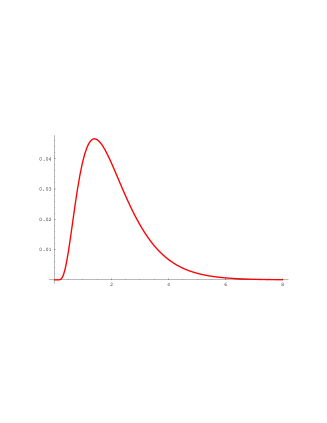
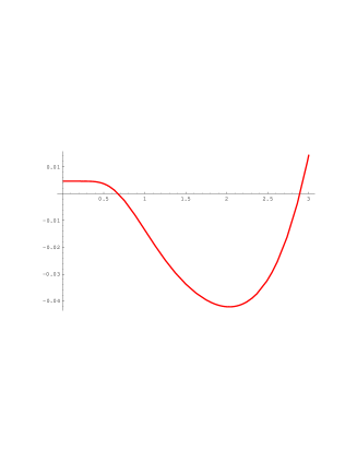
Figure 5: The order parameter for monopole condensation, $|b_{a0}^{(3)}(\tilde{u}_{3})|$ (left) and the effective potential $V_{\rm eff}(\tilde{u}_{3})$ (right), for $\theta_{0}=0$, as a function of the microscopic coupling $\alpha_{0}$.

In the previous discussion, we have chosen a supersymmetry breaking scale smaller than $m$. In fact, for a microscopic coupling $\alpha_{0}<1/2$ or $\alpha_{0}>2$, there are always two singularities on the $\tilde{u}$-plane which are very close to each other, and this decreases the maximum allowed value of $F_{0}$. At very short distances, of the order of $1/m$, the description provided by the Seiberg-Witten effective Lagrangian is no longer valid.

For $\theta_{0}=0$, the microscopic $S$-duality maps the theory with microscopic coupling $\alpha_{0}=g_{0}^{2}/(4\pi)=1/{\rm Im}\tau_{0}$ at the vacuum ${\tilde{u}}$ , to the theory with inverse microscopic coupling $1/\alpha_{0}$ at the vacuum $-\alpha_{0}^{2}{\tilde{u}}$. Since ${\tilde{u}}_{3}(-1/\tau_{0})=\tau_{0}^{2}{\tilde{u}}_{3}(\tau_{0})$, we see that the position of the singularity $\tilde{u}_{3}$ is invariant (up to the modular factor) under $S$-duality. We also have that

$$b_{a0}^{(3)}\left(-\alpha^{2}_{0}\tilde{u}_{3};{1\over\alpha_{0}}\right)=-{1\over\alpha_{0}^{2}}b_{a0}^{(3)}(\tilde{u}_{3};\alpha_{0}).$$ (6.10)

Generically, the effective potential is not left invariant under $S$-duality; but for $\theta_{0}=0$, $V_{\rm eff}(\tilde{u}_{3};1/\alpha_{0})=(1/\alpha_{0}^{4})V_{\rm eff}(\tilde{u}_{3};\alpha_{0})$. The consequence of the microscopic $S$-duality symmetry, in the softly broken theory, is that the physics in the confinement phase is almost the same for the couplings $\alpha_{0}$ and $1/\alpha_{0}$, up to the scaling factor $\alpha_{0}$: the softly broken theory preserves in some way the duality symmetry. This residual symmetry can be seen in figure 5: for the range of values of the coupling constant where the vacuum is stable, there are always two values of the coupling constant which give the same monopole condensate (and hence the same string tension).

When the theory is softly broken down to ${\cal N}=1$ [5], all the possible massive vacua are realized for any value of the coupling constant, and they are permuted by $Sl(2,{\bf Z})$. But, as we have seen, if all the supersymmetries are softly broken down to ${\cal N}=0$, the vacuum degeneracy is lifted in such a way that the theory is locked in a confining phase and the only stable vacua occur for a gauge coupling of order one: the duality symmetry in the phase structure is lost.

6.3 Vacuum structure for $\theta_{0}\not=0$.

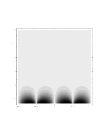
Figure 6: Contour plot of the condensate order parameter $b_{a0}^{(1)}$, evaluated at the singularity $\tilde{u}_{1}$, on the complex plane of the microscopic coupling $\tau_{0}=x+iy$.

In the asymptotically free theories, the $U(1)_{R}$ anomaly relates the theory with microscopic theta angle different from zero with the one at zero angle but where the $u$-plane is rotated (and the rotation angle is proportional to the anomaly). In the self-dual theories, there is no $U(1)_{R}$ anomaly, and the theta angle dependence becomes non-trivial.

As a first approach to unravel the theta angle dependence of the vacuum structure in the softly broken, mass-deformed ${\cal N}=4$ self-dual theory, we obtain the values of the condensate order parameters. The contour plots of figures six to eight show the absolute value of the couplings $b_{a0}^{(i)}$, evaluated at their respective singularities $\tilde{u}_{i}$, for different values of the microscopic coupling $\tau_{0}$ in a range $1/3\leq{\rm Im}\tau_{0}\leq 3$ and $-1\leq{\rm Re}\tau_{0}\leq 1$. Darker zones mean larger absolute values of the condensate order parameter.

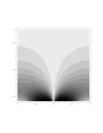
Figure 7: Contour plot of the condensate order parameter $b_{a0}^{(2)}$, evaluated at the singularity $\tilde{u}_{2}$, on the complex plane of the microscopic coupling $\tau_{0}=x+iy$.

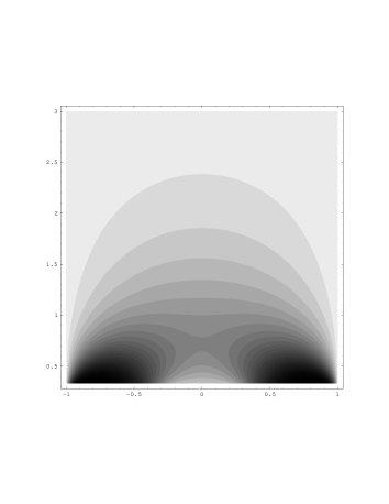
Figure 8: Contour plot of the condensate order parameter $b_{a0}^{(3)}$, evaluated at the singularity $\tilde{u}_{3}$, on the complex plane of the microscopic coupling $\tau_{0}=x+iy$.

At weak coupling (Im$\tau_{0}>3$), all the condensate order parameters are zero for any value of the microscopic angle. This can be understood as a remnant of the microscopic $S$-duality and the results of the previous subsection for zero theta-angle: $S$-duality maps the theory for general angle $\theta_{0}$ to the one with angle $\theta_{0}^{(S)}=-\alpha_{0}^{2}\theta_{0}+{\cal O}(\alpha_{0}^{4})$. Then, for small $\alpha_{0}$, the theory at general $\theta_{0}$ angle is mapped to the one at $(1+\alpha_{0}^{2}\theta_{0}^{2})/\alpha_{0}$ and $\theta_{0}\simeq 0$. This means that at weak coupling and general $\theta_{0}$, there are runaway vacua along $u\rightarrow\infty^{+}$. On the other hand, there is new dynamical information in the strong coupling region: for finite microscopic theta angle, $S$-duality maps strong coupling to strong coupling.

Notice that the plot of $b_{a0}^{(2)}(\tilde{u}_{2})$ in fig. 7 is equivalent to the plot of $b_{a0}^{(3)}(\tilde{u}_{3})$ in fig. 8 with the real axis shifted by one unit. This equivalence is a consequence of the microscopic $T$-duality symmetry, which interchanges the singularities $\tilde{u}_{2}$ and $\tilde{u}_{3}$. In fact, there is more information we can extract from $T$-duality, which tells us that

$$V_{\rm eff}(\tilde{u};\tau_{0}\pm 1)=V_{\rm eff}(\tilde{u};\tau_{0}),$$ (6.11)

therefore

$$V_{\rm eff}(\tilde{u}_{2};\theta_{0}=\pi)=V_{\rm eff}(\tilde{u}_{3};\theta_{0}=\pi).$$ (6.12)

  

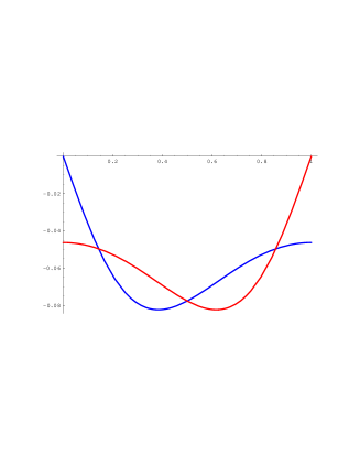
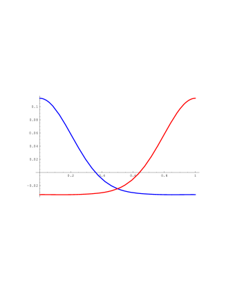
Figure 9: The condensate order parameters $b_{a0}^{(2)}$ and $b_{a0}^{(3)}$ (left) and the effective potential $V_{\rm eff}$ (right) evaluated at their associated singularities $\tilde{u}_{2}$ and $\tilde{u}_{3}$ respectively, as a function of $\theta_{0}/2\pi$, for $\alpha_{0}=3/2$. The level crossing at $\theta_{0}=\pi$ corresponds to two degenerate minima.

We see that, at $\theta_{0}=\pi$, if the vacuum energy is smaller than zero, there must be two equivalent vacua, located at conjugate points on the $\tilde{u}$-plane. Numerically, this happens for $\alpha_{0}{\ \lower-1.2pt\vbox{\hbox{\hbox to0.0pt{$>$\hss}\lower 5.0pt\vbox{\hbox{$\sim$}}}}\ }1$. From the fig. 9, we observe that, when we increase the microscopic angle $\theta_{0}>0$, it appears a condensate around the $\tilde{u}_{2}$ singularity (giving a new local minimum of the effective potential), and that the condensate around $\tilde{u}_{3}$ decreases. At $\theta_{0}=\pi$, both condensates become equivalent and they give the same vacuum energy. The physical electric charge of the BPS states condensing at these two equivalent vacua is exactly zero, but the fact that the CP transformation interchanges the two complex conjugate minima at the plane ${\widetilde{u}}$ is a signal that we have spontaneous CP symmetry breaking. In fact there is a first-order phase transition at $\theta_{0}=\pi$, and for $\pi<\theta_{0}<2\pi$ the absolute minimum is located near the $\tilde{u}_{2}$ singularity. This is another test that the softly broken theory preserves the microscopic $T$-duality symmetry. When $\theta_{0}=2\pi$, the only condensate occurs around the $\tilde{u}_{2}$ singularity, again with zero electric charge, and it is located at the same point that the $\tilde{u}_{3}$ singularity for $\theta_{0}=0$, as it is expected from $T$-duality. A similar behavior has been observed in other softly broken models when a bare theta angle is introduced [10, 31].

When $\alpha_{0}=2$, the singularity $\tilde{u}_{1}$ passes between $\tilde{u}_{2}$ and $\tilde{u}_{3}$. As a result, the monodromy matrices of $\tilde{u}_{1}$ and $\tilde{u}_{2}$ are conjugated . For $\alpha_{0}>2$ and $\theta_{0}\not=n\pi$, the condensate order parameter $b_{a0}^{(1)}(u_{1})$ is different from zero (see fig. 6) and there is a new local minimum near ${\widetilde{u}}_{1}$. But numerically it never becomes the absolute minimum of the effective potential, and the physical vacuum remains located near $\tilde{u}_{2}$ or $\tilde{u}_{3}$ (or it is a degenerate one for $\theta_{0}=\pi$).

Although in the deep strong coupling region ($\alpha_{0}\gg 1$) the singularities $\tilde{u}_{2}$ and $\tilde{u}_{3}$ approach to each other, we have not found any oblique confinement phase at $\theta_{0}=\pi$ (for the allowed values of the supersymmetry breaking parameter). The same negative answer was found in other softly broken ${\cal N}=2$ theories with a bare theta angle [10].

Acknowledgements

We acknowledge L. Álvarez-Gaumé, J.M.F. Labastida and G. Moore for a critical reading of the manuscript. M.M. would like to acknowledge G. Moore for many useful discussions and remarks, and F. Ferrari for useful correspondence. The work of M.M. is supported by DOE grant DE-FG02-92ER4074. The work of F.Z. is supported by a fellowship from Ministerio de Educación y Ciencia.

References

• [1]
• [2] L. Álvarez-Gaumé and S.F. Hassan, “Introduction to S duality in ${\cal N}=2$ supersymmetric gauge theories: a pedagogical review of the work of Seiberg and Witten”, Fortsch. Phys. 45, 159 (1997); hep-th/9701169.
L. Álvarez-Gaumé and F. Zamora, “Duality in quantum field theory (and string theory)”, in ‘The Workshop on Fundamental Particles and Interactions’, Vanderbilt University 1997, and CERN-La Plata-Santiago de Compostela School of Physics 1997, p. 1; hep-th/9709180.
W. Lerche, “Introduction to Seiberg-Witten theory and its stringy origin”, Nucl. Phys. Proc. Suppl. 55B, 83 (1997); hep-th/9611190.
A. Bilal, “Duality in ${\cal N}=2$ $SU(2)$ Yang-Mills theory: a pedagogical introduction to the work of Seiberg and Witten”, hep-th/9601007.
• [3] N. Seiberg and E. Witten, “Electric-magnetic duality, monopole condensation, and confinement in ${\cal N}=2$ supersymmetric Yang-Mills theory”, Nucl. Phys. B426 (1994) 19, hep-th/9407087.
• [4] N. Seiberg and E. Witten, “Monopoles, duality and chiral symmetry breaking in ${\cal N}=2$ supersymmetric QCD”, Nucl. Phys. B431 (1994) 484; hep-th/9408099.
• [5] R. Donagi and E. Witten, “Supersymmetric Yang-Mills theories and integrable systems”, Nucl. Phys. B460 (1996) 299; hep-th/9510101.
• [6] O. Aharony, J. Sonnenschein, M.E. Peskin and S. Yankielowicz, “Exotic non-supersymmetric gauge dynamics from supersymmetric QCD”, Phys. Rev. D52 (1995) 6157; hep-th/9507013.
N. Evans, S.D.H. Hsu and M. Schwetz, “Exact results in softly broken supersymmetric models”, Phys. Lett. B355 (1995) 475; hep-th/9503186.
N. Evans, S.D.H. Hsu, M. Schwetz, S.B. Selipsky, “Exact results and soft breaking masses in supersymmetric gauge theory”, Nucl. Phys. B456 (1995) 205; hep-th/9508002.
• [7] F. Sannino and J. Schechter, “Toy model for breaking super gauge theories at the effective Lagrangian level”, Phys. Rev. D 57 (1998), 170; hep-th/9708113.
• [8] L. Álvarez-Gaumé, J. Distler, C. Kounnas and M. Mariño, “Softly broken ${\cal N}=2$ QCD”, Int. J. Mod. Phys. A11 (1996) 4745, hep-th/9604004;
L. Álvarez-Gaumé and M. Mariño, “Soflty broken ${\cal N}=2$ QCD”, in J.M. Drouffe and J.B. Zuber, eds., The mathematical beauty of physics, World Scientific, 1997; hep-th/9606168.
L. Álvarez-Gaumé and M. Mariño, “More on softly broken ${\cal N}=2$ QCD”, Int. J. Mod. Phys. A12 (1997) 975; hep-th/9606191.
• [9] L. Álvarez-Gaumé, M. Mariño and F. Zamora, “Softly broken ${\cal N}=2$ QCD with massive quark hypermultiplets, I”, Int. J. Mod. Phys. A13 (1998) 403; hep-th/9703072.
“Softly broken ${\cal N}=2$ QCD with massive quark hypermultiplets, II”, hep-th/9707072.
• [10] N. Evans, S.D.H. Hsu and M. Schwetz, “Phase transitions in softly broken ${\cal N}=2$ QCD at nonzero $\theta$ angle,” Nucl. Phys. B484 (1997) 124; hep-th/9608135.
• [11] J. Maldacena, “The large N limit of superconformal field theories and supergravity”; hep-th/9711200.
• [12] N. Dorey, V. V. Khoze and M. P. Mattis, “On ${\cal N}=2$ supersymmetric QCD with four flavors”, Nucl. Phys. B492 (1997) 607; hep-th/9611016.
• [13] N. Dorey, V. Khoze and M. Mattis, “On mass-deformed ${\cal N}=4$ supersymmetric Yang-Mills theory”, Phys. Lett. B 396 (1997) 141; hep-th/9612231.
• [14] F. Ferrari, “The dyon spectra of finite gauge theories”, Nucl. Phys. B501 (1997) 53; hep-th/9702166.
• [15] G. Moore and E. Witten, “Integration over the $u$-plane in Donaldson theory”, hep-th/9709193.
• [16] A. Losev, N. Nekrasov and S. Shatashvili, “Issues in topological gauge theory”, hep-th/9711108; “Testing Seiberg-Witten solution”; hep-th/9801061.
• [17] M. Mariño and G. Moore, “Integrating over the Coulomb branch in ${\cal N}=2$ supersymmetric gauge theory”, hep-th/9712062.
• [18] G. Carlino, K. Konishi and H. Terao, “Quark number fractionalization in ${\cal N}=2$ supersymmetric $SU(2)\times U(1)^{N_{f}}$ gauge theories”, hep-th/9801027.
• [19] N.I. Akhiezer, Elements of the theory of elliptic functions, AMS, 1990.
• [20] A. Bilal and F. Ferrari, “The BPS spectra and superconformal points in massive ${\cal N}=2$ supersymmetric QCD”; hep-th/9706145.
• [21] M. Matone, “Instantons and recursion relations in ${\cal N}=2$ supersymmetric gauge theories”, Phys. Lett. B357 (1995) 342; hep-th/9506102.
J. Sonnenschein, S. Theisen and S. Yankielowicz, “On the relation between the holomorphic prepotential and the quantum moduli in supersymmetric gauge theories”, Phys. Lett. B367 (1996) 145; hep-th/9510129.
T. Eguchi and S.-K. Yang, “Prepotentials of ${\cal N}=2$ supersymmetric gauge theories and soliton equations”, Mod. Phys. Lett. A11 (1996) 131; hep-th/9510183.
E. D’Hoker, I.M. Krichever and D.H. Phong, “The renormalization group equation in ${\cal N}=2$ supersymmetric gauge theories”, Nucl. Phys. B494 (1997) 89; hep-th/9610156.
• [22] E. D’Hoker and D.H. Phong, “Calogero-Moser systems in $SU(N)$ Seiberg-Witten theory”; hep-th/9709053.
• [23] J.A. Minahan, D. Nemeschansky and N.P. Warner, “Instanton expansions for mass-deformed ${\cal N}=4$ super Yang-Mills theories”; hep-th/9710146.
• [24] P.C. Argyres, M.R. Plesser and A.D. Shapere, “The Coulomb phase of ${\cal N}=2$ supersymmetric QCD”, Phys. Rev. Lett. 75 (1995) 1699; hep-th/9505100.
• [25] P.C. Argyres and A.D. Shapere, “The vacuum structure of ${\cal N}=2$ super-QCD with classical gauge groups”, Nucl. Phys. B461 (1996) 437; hep-th/9509175.
• [26] A. Hanany and Y. Oz, “On the quantum moduli space of ${\cal N}=2$ supersymmetric $SU(N_{c})$ gauge theories”, Nucl. Phys. B452 (1995) 283; hep-th/9505075.
• [27] A. Hanany, “On the quantum moduli space of vacua of ${\cal N}=2$ supersymmetric gauge theories”, Nucl. Phys. B466 (1996) 85; hep-th/9509176.
• [28] J.A. Minahan and D. Nemeschansky, “Hyperelliptic curves for supersymmetric Yang-Mills”, Nucl. Phys. B464 (1996) 3; hep-th/9507032.
J.A. Minahan and D. Nemeschansky, “${\cal N}=2$ super Yang-Mills and subgroups of $SL(2,{\bf Z})$”, Nucl. Phys. B468 (1996) 72; hep-th/9601059.
• [29] A. Gorsky, A. Marshakov, A. Mironov and A. Morozov, “RG equations from Whitham hierarchy”, hep-th/9802007.
• [30] G. ’t Hooft, “Topology of the gauge condition and new confinement phases in non-abelian gauge theories”, Nucl. Phys. B190 (1981) 455.
• [31] K. Konishi, “Confinement, supersymmetry breaking and theta parameter dependence in the Seiberg-Witten model”, Phys. Lett. B392 (1997) 101; hep-th/9609021.
K. Konishi and H. Terao, “CP, charge fractionalizations and low-energy effective actions in the $SU(2)$ Seiberg-Witten theories with quarks”, hep-th/9707005.