hep-th/9804034
PUPT-1784
Is Physics in the Infinite Momentum Frame Independent of the Compactification Radius?

With the aim of clarifying the eleven dimensional content of Matrix theory, we examine the dependence of a theory in the infinite momentum frame (IMF) on the (purely spatial) longitudinal compactification radius $R$.

It is shown that in a point particle theory the generic scattering amplitude becomes independent of $R$ in the IMF. Processes with zero longitudinal momentum transfer are found to be exceptional. The same question is addressed in a theory with extended objects. A one-loop type II string amplitude is shown to be $R$-independent in the IMF, and to coincide with that of the uncompactified theory. No exceptional processes exist in this case.

The possible implications of these results for M-theory are discussed. In particular, if amplitudes in M-theory are independent of $R$ in the IMF, Matrix theory can be rightfully expected (in the $N\to\infty$ limit) to describe uncompactified M-theory.

PACS codes: 11.25.w, 11.25.Db, 11.80.m, 11.30.Cp

June 1998

1 Introduction

Dramatic advances in recent years have led to the realization that a consistent eleven dimensional quantum theory of gravity, M-theory, should exist [1]. Over a year ago Banks, Fischler, Shenker and Susskind [2] (BFSS) made the bold conjecture that M-theory in the infinite momentum frame (IMF) [3] has a precise description as a particular limit of a matrix quantum mechanical system. The system in question was originally obtained as a description of D0-brane physics in ten dimensional string theory [4, 5].

For the definition of the model, the longitudinal direction is compactified on an auxiliary (spatial) circle of radius $R$; the total longitudinal momentum is then quantized, $P=N/R$. The physics of uncompactified M-theory is expected to be recovered in the $N,R,N/R\to\infty$ limit. Several rather remarkable pieces of evidence were presented for the conjecture in [2], and others followed, but progress was hampered by the technical difficulty of studying the large $N$ limit.

The situation improved last year when Susskind [8] conjectured that even the finite $N$ Matrix model should have direct physical meaning as the discrete light cone quantization (DLCQ) [9] of M-theory. In that case the description is in terms of an ordinary (as opposed to infinite momentum) reference frame, and the compact direction is null, with radius $R^{\prime}$. This form of the conjecture allowed several more stringent tests, by comparison of the Matrix amplitudes with those in the DLCQ of supergravity. If Susskind’s conjecture were correct, the $N,R^{\prime}\to\infty$ limit of the model, with $N/R^{\prime}$ fixed, would be expected to yield the standard (uncompactified) light front quantization (LFQ) of M theory.

In another important paper, Seiberg [10] constructed a seemingly miraculous proof that the finite $N$ Matrix model indeed describes the DLCQ of M-theory. This, however, was done at the cost of defining DLCQ as being Lorentz related to an IMF compactification on a vanishingly small spatial circle. As a result, the question of whether the model captures eleven dimensional physics is greatly obscured. The large $N$ limit of such a DLCQ would be equivalent to the BFSS limit, but with a spatial radius $R\to 0$ instead of $R\to\infty$. We will henceforth refer to Seiberg’s limit as ‘near DLCQ’ to distinguish it from the conventional DLCQ [9]. That this is the useful way to interpret what is meant by DLCQ in the context of the Matrix model is evidenced by the success of [10] (see also [11]) in providing a uniform prescription for toroidal compactifications.

At about the same time, some discrepancies between Matrix model and supergravity scattering amplitudes were found [12]. (Difficulties for Matrix model amplitudes in nontrivial backgrounds have also been reported [13].) The status of the model is therefore at present uncertain, and there has been some controversy in the literature regarding what it is exactly that Seiberg proved, and whether or not Matrix theory and supergravity amplitudes should be directly compared.

To gain additional insight, Hellerman and Polchinski [14] examined the limit of a field theory compactification on an almost lightlike circle (or equivalently, on a vanishingly small spatial circle in the IMF), at fixed $N$. They found the limit to be complicated: the longitudinal zero modes become strongly coupled, and as a result, in almost all theories some of the perturbation theory amplitudes diverge. As a consequence of this, the authors of [14] expressed serious doubts regarding the relevance of the Matrix model for describing uncompactified M-theory. In particular, they emphasized that amplitudes in finite $N$ Matrix theory and supergravity do not have, a priori, a common range of validity.

De Alwis [15] has used the scaling limits of [10] to argue that finite $N$ Matrix model and supergravity amplitudes (with one impact parameter and no longitudinal momentum transfer) should be expected to agree as a result of string world-sheet duality.

More recently, Kabat and Taylor [16] have explicitly shown that there is a precise correspondence between a subset of the terms in the one loop Matrix theory potential and the linearized DLCQ supergravity potential arising from exchange of quanta with zero longitudinal momentum. These authors also point out, however, that the finite $N$ Matrix model violates the equivalence principle. At finite $N$, then, Matrix theory and DLCQ supergravity are distinct. As a consequence of this, the authors of [16] espouse the view that near DLCQ M-theory is not described at low energies by near DLCQ supergravity. This possibility has also been taken seriously by Banks [6] and Susskind [7]. The latter author suggests that amplitudes computed in the finite $N$ Matrix model and near DLCQ supergravity will agree only for special processes, presumably protected by a supersymmetry nonrenormalization theorem which allows a continuation from the Matrix model to the supergravity regime.

An alternative resolution has been advocated by Douglas and Ooguri [13]. This is that the DLCQ Lagrangian is renormalized in a nontrivial manner when modes with zero longitudinal momentum are integrated out. If this were correct, it should be possible to find a modified Lagrangian which yields an adequate description of the physics.

Even though the widespread hope remains that the above difficulties of the finite $N$ model will be removed as $N\to\infty$, Banks [6] has recognized the possibility that the large $N$ limit of near DLCQ M-theory might not converge to the eleven dimensional theory.

Susskind [7], on the other hand, has argued that near DLCQ M-theory is, in the large $N$ limit, able to capture eleven dimensional physics, in spite of the fact that in the IMF it is manifestly defined as a compactification on a zero size spatial circle. His point is simply that an object of proper longitudinal size $L$ is Lorentz contracted to a size $\propto LR/N$ in a frame where its longitudinal momentum is $N/R$ ($R$ being the radius of the spatial circle). Clearly this size can be made arbitrarily smaller than $R$ for large $N$.

Balasubramanian, Gopakumar and Larsen [17] have given a very precise discussion of the limits involved in the definition of the Matrix model and have provided additional evidence for the possibility of recovering the full uncompactified theory in the large $N$ limit. In particular, they examine a classical solution of eleven dimensional supergravity with a compactified longitudinal direction of radius $R$, carrying $N$ units of momentum in the compact direction. They discover that, even for $R\to 0$, the physical size of the circle, as measured in the supergravity metric, can be made arbitrarily large (for all finite transverse distances) by increasing $N$. This establishes at least the self-consistency of the supergravity solution in this limit.

On top of this, Bilal [18] has analyzed a string theory one-loop amplitude in the near DLCQ limit, finding it to have a well-defined, finite limit. This raises the hope that the situation in M-theory might be simpler than that discussed in [14] for field theory. The crucial difference between the string and field theory cases is the existence of string winding modes.

Despite all of this, a skeptic might remain unconvinced. Arguments based on Lorentz contraction might work out differently in a theory with extended objects, which can wrap around the compact direction. Also, the case might be made that the self-consistency of a supergravity solution is logically independent from the recovery of the full eleven dimensional M-theory.

The essence of the matter is that there is a potential contradiction in some of the recent attempts to clarify the significance of Matrix theory: on the one hand, a proof of the validity of the Matrix model based on knowledge gained from perturbative type IIA string theory requires $R$ to be small; on the other hand, for the model to describe uncompactified M-theory it would seem necessary to let $R\to\infty$ [2]. Even if this is done in two separate steps, as in the near DLCQ program [8, 10] (first let $R\to 0$ at fixed $N$, then take $N,R^{\prime}\to\infty$), arguments which suggest that the large $N$ Matrix model describes eleven dimensional M-theory [7, 17] are at risk of being in conflict with Seiberg’s proof [10], which is based on the understanding that, for any $N$, the Matrix model describes M-theory in the IMF, compactified on a vanishingly small spatial circle. Consequently, the question of whether Matrix theory provides information about uncompactified M-theory seems to merit further discussion. That is the general motivation for the present paper.

If we are to believe that a theory which in the IMF is compactified on a vanishingly small circle can capture (in the large $N$ limit) the physics of the same theory with no compactification, then it seems inevitable that a compatification in the IMF of any finite size should also do so. Any of the decompactification arguments advanced for the case of $R=0$ would certainly apply for any other value of $R$. Unless there are several uncompactified limits of the theory, one is led to the conclusion that physics in the IMF for such a theory must be independent of the compactification radius. (The authors of [17] have also arrived at this conjecture.) This is the specific question that we investigate in what follows.

We will begin by giving, in Section 2, a precise specification of the limits that concern us. In Section 3 we then attempt to analyze the problem for a theory of point particles; we consider scalar field theory as a concrete example. In Section 4 we reexamine this issue in a theory with extended objects, string theory. We conclude in Section 5 with some discussion on the possible implications of our results for the case of M-theory.

2 Boosting to the Infinite Momentum Frame

We wish to consider the amplitude for a scattering event in a (Lorentz invariant) theory defined in $D$ spacetime dimensions. The situation will be analyzed from the vantage point of different Lorentz frames, related by boosts along what we will call the longitudinal direction. Specifically, we introduce a frame $F^{\prime}$, and a family of frames $F_{\epsilon}$, indexed by a parameter $\epsilon\ll 1$, and related to $F^{\prime}$ by a boost with rapidity parameter $\omega=\ln(\sqrt{2}/\epsilon)$, i.e. $\beta=\tanh\omega$ is given by $\beta\approx 1-\epsilon^{2}$. As $\epsilon\to 0$, $F_{\epsilon}$ approaches the IMF. By this we simply mean that all longitudinal momenta in $F_{\epsilon}$ become arbitrarily larger than any other scale in the problem. With this understanding, we will loosely refer to $F_{\epsilon}$ as the IMF. If the theory is quantized on an equal time surface in $F_{\epsilon}$, then as $\epsilon\to 0$ the quantization surface approaches a light front surface in $F^{\prime}$. Because of this we will refer to $F^{\prime}$ as the light front quantization (LFQ) frame.

Notice that there is in our discussion a clear distinction between the IMF and the LFQ frame, whereas both terms are sometimes used interchangeably in the literature. In particular, the momenta of localized objects involved in the scattering process are fixed and finite in the LFQ frame $F^{\prime}$. Of course, the same physics should be visible from the point of view of either frame (even though, as a result of the compactification which will be introduced below, longitudinal boosts are not a symmetry of the theory).

Following Seiberg [10], we compactify the longitudinal direction in $F_{\epsilon}$, $x^{1}$, on a circle of radius $R$,

$${x^{0}\choose x^{1}}\sim{x^{0}\choose x^{1}}+2\pi R{0\choose 1}.$$ (1)

In terms of $F^{\prime}$ light front coordinates $x^{\prime\pm}=(x^{\prime 0}\pm x^{\prime 1})/\sqrt{2}$ this is

$${x^{\prime+}\choose x^{\prime-}}\sim{x^{\prime+}\choose x^{\prime-}}+2\pi R^{\prime}{\epsilon^{2}/2\choose-1},$$ (2)

where we have defined $R^{\prime}=R/\epsilon$. In $F^{\prime}$, then, the compactification is almost along $x^{\prime-}$, with radius $R^{\prime}$.

The longitudinal momentum in $F_{\epsilon}$ is quantized; let $P=N/R$ be the total initial longitudinal momentum for the scattering event. In $F^{\prime}$ this corresponds to the statement that the generator of $x^{\prime-}$ translations (at fixed $x^{\prime+}$) is quantized (up to $\mathcal{O}(\epsilon^{2})$ terms), ${P^{\prime}}^{+}=-P^{\prime}_{-}=N/R^{\prime}$. The situation is summarized in Fig. 1.

Figure 1: Relation between the IMF $F_{\epsilon}$, and the LFQ frame $F^{\prime}$. The arrow indicates a longitudinal boost.

We should emphasize that the compactification depends on $\epsilon$ not only because the proper length of the circle, $2\pi R$, might be $\epsilon$-dependent (see below), but also because the frame $F_{\epsilon}$ where the circle is purely spatial is different for different values of $\epsilon$.

Now, by construction, $\epsilon\to 0$ is the IMF (or LFQ) limit. There are, however, several ways of taking this limit. We will be interested in the following three:

• BFSS (uncompactified IMF) limit: $\epsilon\nolinebreak\to\nolinebreak 0$ with $N\nolinebreak\to\nolinebreak\infty$, $R\nolinebreak\to\nolinebreak\infty$, $N/R\nolinebreak\to\nolinebreak\infty$. Then $R^{\prime}=\epsilon^{-1}R\to\infty$.

• Compactified IMF limit: $\epsilon\nolinebreak\to\nolinebreak 0$ with $N\nolinebreak\to\nolinebreak\infty$, $R$ fixed. Then $R^{\prime}=\epsilon^{-1}R\nolinebreak\to\nolinebreak\infty$.

• Seiberg-Susskind (near DLCQ) limit: $\epsilon\nolinebreak\to\nolinebreak 0$ with $N,R^{\prime}$ fixed. Then $R=\epsilon R^{\prime}\nolinebreak\to 0$, $N/R=\epsilon^{-1}N/R^{\prime}\nolinebreak\to\nolinebreak\infty$.

Notice that, from (2), we need $R^{\prime}\epsilon^{2}\to 0$ in order for the compactification in $F^{\prime}$ to converge to one at fixed $x^{\prime+}$. This gives for limit 1 the additional requirement $R\propto\epsilon^{-\alpha}$ with $0<\alpha<1$, and therefore $N\propto\epsilon^{-\beta}$, with $\beta>\alpha$. We should perhaps stress that in limits 1 and 2 the circle does not become null as $\epsilon\to 0$.

In the first two limits, the behavior of $N/R^{\prime}$ depends on the nature of the scattered objects. The simplest case is that with objects which are localized in the longitudinal direction. Then $N/R^{\prime}$ should be fixed and finite. This implies $N/R\propto\epsilon^{-1}$ in limit 1 (i.e. $\beta=\alpha+1$), and $N\propto\epsilon^{-1}$ in limit 2.

For an extended longitudinally wrapped object, on the other hand, it is not the momentum $N/R^{\prime}$, but the momentum density, $N/R^{\prime 2}$, that should be fixed and finite. For limits 1 and 2 this means $N/R\propto\epsilon^{-2}$ ($\beta=\alpha+2$) and $N\propto\epsilon^{-2}$, respectively. (To be absolutely clear we remark that the above relations between $N$ and $\epsilon$ give only the leading small $\epsilon$ behavior.)

In the case of limit 3, we imagine that $R^{\prime}\to\infty$ after $\epsilon\to 0$. Then $N\to\infty$, again with two possible choices for the behavior of $N/R^{\prime}$.

It is evident that limit 1 yields the uncompactified theory. The situation is not so clear for limit 2. There $R^{\prime}\to\infty$, but $R$ is fixed. Which is it that is relevant? Things are even worse for limit 3. Even if we let $R^{\prime}\to\infty$, we have taken $R\to 0$ to begin with. So again, which is the physically significant radius?

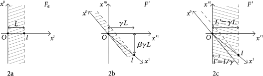
Figure 2: Decompactifying by boosting?

To try to answer this question, consider Fig. 2. Fig. 2a shows the $(x^{0},x^{1})$ plane in $F_{\epsilon}$, where the periodic identification is at constant $x^{0}$. So, for example, the origin $O$ and the event $I$, a distance $L=2\pi R$ away, are identified. The shaded area is a physical slice of the covering space; all events in the compactified spacetime are included in this slice exactly once. Fig. 2b shows events $O$ and $I$, and the same physical slice, in $F^{\prime}$. The periodic identification now involves shifts by $\gamma L$ along $x^{\prime 1}$, and by $-\gamma\beta L$ along $x^{\prime 0}$. Fig. 2c also shows $F^{\prime}$, but with a different, equally valid, choice of physical slice, one which is parallel to the $x^{\prime 0}$ axis. From the figure it is easy to convince oneself that this slice also contains all physical events exactly once. To avoid confusion, we emphasize that the periodic identification in this slice is still made diagonally, not horizontally.

Now, the point is that in Fig. 2c the ‘spatial extent’ of the slice as seen in $F^{\prime}$ is $L^{\prime}=\gamma L$, which can be made arbitrarily large. Since $\gamma=\cosh\omega\approx\epsilon^{-1}/\sqrt{2}\to\infty$, this is precisely what allows $L^{\prime}\to\infty$ for limit 2, and $L^{\prime}$ fixed in spite of $L\to 0$ in limit 3.

Notice that this seems to be the opposite of Lorentz contraction. That is to say, if an object of proper length $l$ just slightly shorter than $L$ were to be placed at rest along the $x^{1}$-axis in $F_{\epsilon}$, with its left end at the origin, then its length in $F^{\prime}$ would be $l^{\prime}=l/\gamma$, a factor $\gamma^{2}$ shorter than $L^{\prime}$ (see Fig. 2c). But by the very definition of the IMF, there is no object at rest in $F_{\epsilon}$, so this should be stated the other way around: an object of proper length $s^{\prime}\ll L^{\prime}$ at rest in $F^{\prime}$ has length $s=s^{\prime}/\gamma\ll L$ in $F_{\epsilon}$. (This is essentially Susskind’s Lorentz contraction argument [7].)

Something very perplexing is going on here. On the one hand, Fig. 2 seems to indicate that a space can be decompactified by a large boost. On the other hand, the proper length of the circle, $L=2\pi R$, is of course Lorentz invariant.

Let us now suggest that, in a point particle theory, the relevant criterion for decompactification should be that the Compton wavelengths of all particles be, in the IMF, much smaller than the spatial radius $R$. But by the above Lorentz contraction argument this is accomplished automatically as $N\to\infty$, independently of $R$. It is then plausible to expect scattering amplitudes in a point particle theory to be independent of $R$ in this limit. We explore this possibility in Section 3. We stress that this expectation is not in any obvious way related to the well-known irrelevance of the (frame-dependent) radius of the null circle in DLCQ amplitudes. $R$ in our discussion is defined in $F_{\epsilon}$ as a purely spatial radius.

In a theory with extended objects, on the other hand, the proper length of the circle could possibly be ‘felt’ by longitudinally wrapped objects. In particular, the mass of such an object should be $R$-dependent. One might then expect amplitudes in such a theory to depend on $R$ even in the large $N$ limit. We will examine this in Section 4.

3 Field Theory Amplitudes

We now study the $R$-dependence of $D$ dimensional field theory scattering amplitudes in the IMF $F_{\epsilon}$. For concreteness, we will focus on the case of a scalar field; our arguments should be easy to generalize.

Consider a scattering process with $A$ initial and $B$ final particles of momenta $\{K^{M}_{a}\}$. Here $a=1,\ldots,A+B$ is a particle label, and $M=0,1,\ldots,D-1$ a coordinate index. We split the external momenta into longitudinal and transverse parts according to $K^{M}_{a}=(K^{0}_{a},K^{1}_{a},K^{i}_{a})=(E_{a},P_{a},\vec{Q}_{a})$, where $i=2,\ldots,D-1$ (and $x^{1}$ is the compact direction). We take all $E_{a}>0$; in other words, the initial (final) external legs are incoming (outgoing). Due to the compactification, all longitudinal momenta are quantized, $P_{a}=N_{a}/R$. By the definition of the IMF, $N_{a}>0\;\forall\;a$. Let $N=\sum_{a=1}^{A}N_{a}$; then $P=N/R$ is the total (initial) longitudinal momentum. We will examine the compactified IMF limit $\epsilon\to 0$ with $N\to\infty$, $R$ fixed (and therefore $P\to\infty$) of the amplitude. The fraction of longitudinal momentum of each external leg, $\zeta_{a}=N_{a}/N$, is held fixed as $N\to\infty$.

The first thing to notice is that kinematic Lorentz invariants $K_{a}\cdot K_{b}$ could just as well be evaluated in $F^{\prime}$, where they are finite. So when evaluated in $F_{\epsilon}$, to leading order in $N$ they can only depend on ratios of longitudinal momenta, and are therefore independent of $R$. This already guarantees that all tree level diagrams in the IMF do not depend on $R$.

The situation could appear to be different for loop diagrams, which include sums over the longitudinal momenta carried by intermediate lines, weighted by explicit factors of $1/R$. As usual in IMF (or LFQ) physics, things are more transparent in old-fashioned perturbation theory (OFPT) language [3].

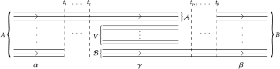
Figure 3: Arbitrary old-fashioned perturbation theory diagram. $\alpha$, $\beta$, and $\gamma$ denote the initial, final and intermediate state, respectively.

Consider then the arbitrary OFPT diagram shown in Fig. 3. In some intermediate state (between two interaction times $t_{\gamma}$, $t_{\gamma+1}$) the diagram has $I$ particle lines, of which $\mathcal{A}$ ($\mathcal{B}$) are external initial (final) lines. Relabel these so that they have momenta $K^{M}_{a}$, $a=A-\mathcal{A}+1,\ldots,A$ ($a=A+1,\ldots,A+\mathcal{B}$). The remaining $V=I-\mathcal{A}-\mathcal{B}$ lines of the intermediate state correspond to internal (i.e. virtual) particles with momenta $k^{M}_{a}=(e_{a},p_{a},\vec{q}_{a})$, $a=1,\ldots,V$. Here $p_{a}=n_{a}/R$; define the longitudinal fraction $\eta_{a}=n_{a}/N$. Notice $n_{a}$ and $\eta_{a}$ are not necessarily positive. The energy difference between the initial state $\alpha$ and an intermediate state $\gamma$ with a particlular choice of $\eta_{a}$ is

$$E_{\alpha}-E_{\gamma}=\sum\limits_{a=1}^{A}\sqrt{\zeta_{a}^{2}P^{2}+\vec{Q}_{a}^{2}}-\sum\limits_{a=A-\mathcal{A}+1}^{A+\mathcal{B}}\sqrt{\zeta_{a}^{2}P^{2}+\vec{Q}_{a}^{2}}-\sum\limits_{a=1}^{V}\sqrt{\eta_{a}^{2}P^{2}+\vec{q}_{a}^{\,2}}.$$ (3)

Such a state would thus contribute to the amplitude a factor

$$f(P,\eta_{a}) = \prod_{a=1}^{V}\left(\frac{1}{2\sqrt{\eta_{a}^{2}P^{2}+\vec{q}_{a}^{\,2}}}\right)$$

$$\times\;\frac{1}{\sum\limits_{a=1}^{A-\mathcal{A}}\sqrt{\zeta_{a}^{2}P^{2}+\vec{Q}_{a}^{2}}-\sum\limits_{a=A+1}^{A+\mathcal{B}}\sqrt{\zeta_{a}^{2}P^{2}+\vec{Q}_{a}^{2}}-\sum\limits_{a=1}^{V}\sqrt{\eta_{a}^{2}P^{2}+\vec{q}_{a}^{\,2}}}.$$

The total factor associated with the state is therefore (omitting the integrals over the transverse momenta $\vec{q}_{a}$)

$$F_{N}(R)=\left(\frac{1}{R}\right)^{V}\sum_{n_{1}=-\infty}^{+\infty}\cdots\sum_{n_{V}=-\infty}^{+\infty}R\ \delta_{N_{\alpha},N_{\gamma}}\ f\left(\frac{N}{R},\frac{n_{a}}{N}\right),$$ (5)

where the Kronecker delta enforces longitudinal momentum conservation,

$$N_{\alpha}-N_{\gamma}=\sum\limits_{a=1}^{A-\mathcal{A}}N_{a}-\sum\limits_{a=A+1}^{A+\mathcal{B}}N_{a}-\sum\limits_{a=1}^{V}n_{a}=0.$$ (6)

Now, as $N\to\infty$ with $N_{a}\propto N$, (6) shows that in the generic case at least one of the $n_{a}$ must scale like $N$. An exception to this occurs if it so happens that $\sum_{a=1}^{A-\mathcal{A}}N_{a}=\sum_{a=A+1}^{A+\mathcal{B}}N_{a}$. Let us discuss the generic situation for now; we will return to the exceptional case below.

Any one term in the sum (5), with all (but one) $n_{a}$ fixed, vanishes in the large $N$ limit. To properly examine the limit, then, focus attention on terms in which all $n_{a}$ scale like $N$ (all $\eta_{a}$ are then held fixed). It is straightforward to verify that the dominant contribution to $F_{N}(R)$ comes from those states with $n_{a}\geq 0\ \forall\ a=1,\ldots,V$. For these the leading terms in the energy difference denominator in (3) cancel. States with negative $n_{a}$ are suppressed by an additional factor of $(N/R)^{-2}$. This is just the usual decoupling of negative momentum states in the IMF [3]. Omitting these, rewriting the sums in terms of $\eta_{a}$, and replacing $R$ by $N\cdot R/N$, we have

$$F_{N}(R)=\left(\frac{1}{N}\right)^{V}\sum_{\eta_{1}=0,\frac{1}{N},\ldots}^{1}\cdots\sum_{\eta_{V}=0,\frac{1}{N},\ldots}^{1}\left(\frac{N}{R}\right)^{V-1}N\delta_{N_{\alpha},N_{\gamma}}\ f\left(\frac{N}{R},\eta_{a}\right).$$ (7)

The point is now simply that as $N\to\infty$, the sums converge to integrals of a finite integrand. To make this clear, define a sequence of step-functions $\{g_{N}(R,\eta_{a})\}$ by

$${g_{N}(R,\eta_{a})=\left(\frac{N}{R}\right)^{V-1}f\left(\frac{N}{R},\frac{\left[N\eta_{a}\right]}{N}\right),}$$ (8)

where $[N\eta_{a}]$ denotes the integral part of $N\eta_{a}$. Then (7) can be written as an integral,

$$F_{N}(R)=\int\limits_{0}^{1+1/N}d\eta_{1}\cdots\int\limits_{0}^{1+1/N}d\eta_{V}\ N\delta_{N_{\alpha},N_{\gamma}}\ g_{N}(R,\eta_{a}).$$ (9)

As $N\to\infty$, the sequence $g_{N}(R,\eta_{a})$ converges almost everywhere to the function

$${g_{\infty}(\eta_{a})=\prod_{a=1}^{V}\left(\frac{1}{2\eta_{a}}\right)\frac{2}{\sum\limits_{a=1}^{A-\mathcal{A}}\zeta_{a}^{-1}\vec{Q}_{a}^{2}-\sum\limits_{a=A+1}^{A+\mathcal{B}}\zeta_{a}^{-1}\vec{Q}_{a}^{2}-\sum\limits_{a=1}^{V}\eta_{a}^{-1}\vec{q}_{a}^{\,2}}},$$ (10)

and $N\delta_{N_{\alpha},N_{\gamma}}$ becomes a delta function. Consequently, $F_{N}(R)$ converges to the $R$-independent factor

$${F_{\infty}=\int\limits_{0}^{1}d\eta_{1}\cdots\int\limits_{0}^{1}d\eta_{V}\ \delta(\sum\limits_{a=1}^{A-\mathcal{A}}\zeta_{a}-\sum\limits_{a=A+1}^{A+\mathcal{B}}\zeta_{a}-\sum\limits_{a=1}^{V}\eta_{a})\ g_{\infty}(\eta_{a})}.$$ (11)

We have ignored here possible subtleties in exchanging the limit and the integrals, as well as in regularizing the integrals. Nonetheless, the final result is eminently reasonable, since it amounts to the usual cancellation of factors of $P$ in IMF diagrams that yields finite perturbation theory rules (matching those of LFQ), coupled with the standard conversion of sums into integrals in the large $N$ limit.

We have thus shown that generic IMF scattering amplitudes in a point particle theory are independent of the IMF compactification radius, as conjectured in Section 2. To be precise, we emphasize that we are discussing here the compactified IMF limit $N\to\infty$ with $R$ fixed. The large $N$ limit is essential; it has the double effect of forcing $P\to\infty$ and turning the sums into integrals. The essence of the matter is very simple: in this limit, the amplitudes are functions of $R$ only through the combination $N/R$, so all dependence on $R$ drops out for large $N$.

It is important to note that expression (11) agrees precisely with the intermediate state factor that would be obtained with standard IMF (or LFQ) perturbation theory rules [3] in the uncompactified theory.

The situation is quite different, however, in the exceptional case where the external lines which appear in the intermediate state are such that $\sum_{a=1}^{A-\mathcal{A}}N_{a}=\sum_{a=A+1}^{A+\mathcal{B}}N_{a}$. For this case, as can be seen from (6), the kinematics forces the total internal momentum to vanish, $\sum_{a=1}^{V}n_{a}=0$, and the $n_{a}$ need not scale with $N$. Any one term in the sum (5), with all $n_{a}$ fixed, converges to a finite value as $N\to\infty$,

$$\left(\frac{1}{R}\right)^{V-1}f\left(\frac{N}{R},\frac{n_{a}}{N}\right)\to\prod_{a=1}^{V}\left(\frac{1}{2\sqrt{\left(\frac{n_{a}}{R}\right)^{2}+\vec{q}_{a}^{\,2}}}\right)\frac{1}{-\sum\limits_{a=1}^{V}\sqrt{\left(\frac{n_{a}}{R}\right)^{2}+\vec{q}_{a}^{\,2}}}.$$ (12)

In this case, then, lines with negative longitudinal momentum do not decouple, and there is some remaining $R$-dependence even for $N\to\infty$.

A particular example of this exceptional case is a diagram recently examined by Hellerman and Polchinski [14]. They consider a $2\to 2$ one-loop covariant diagram with no longitudinal momentum exchange, in $\phi^{4}$-theory, and find that it diverges in the Seiberg-Susskind limit, $R\to 0$ at fixed $N$. This can of course be seen directly in OFPT language.

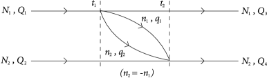
Figure 4: An ‘exceptional’ OFPT one-loop diagram.

Fig. 4 shows a particular time ordering of the one-loop covariant diagram in [14]. In our notation (using $n_{2}=-n_{1}$), the intermediate state contributes a total factor

$$F_{N}(R) = \frac{1}{R}\sum_{n_{1}=-\infty}^{\infty}\frac{1}{2\sqrt{\left(\frac{n_{1}}{R}\right)^{2}+\vec{q}_{1}^{\,2}}}\,\frac{1}{2\sqrt{\left(\frac{n_{1}}{R}\right)^{2}+\vec{q}_{2}^{\,2}}}$$

$$\times\>\frac{1}{\sqrt{\left(\frac{N_{1}}{R}\right)^{2}+\vec{Q}_{1}^{2}}-\sqrt{\left(\frac{N_{1}}{R}\right)^{2}+\vec{Q}_{3}^{2}}-\sqrt{\left(\frac{n_{1}}{R}\right)^{2}+\vec{q}_{1}^{\,2}}-\sqrt{\left(\frac{n_{1}}{R}\right)^{2}+\vec{q}_{2}^{\,2}}}.$$

As $R\to 0$ with all $N_{a}$ fixed, all terms in the sum with $n_{1}\neq 0$ vanish ($\propto R^{2}$), but the zero mode term with $n_{1}=0$ diverges ($\propto R^{-1}$). This is what was found in [14]. In the compactified IMF limit $N\to\infty$ with $R$ fixed (and $N_{a}\propto N$), on the other hand, each term in the sum converges to a finite limit, as stated before. $F_{\infty}(R)$ itself is then finite (for $R>0$) and $R$-dependent. Physically, the kinematics is such that, even in the IMF, virtual states are allowed to have particle lines with small longitudinal momentum. These particles have arbitrarily large Compton wavelengths, and can therefore ‘feel’ the size of the compactification circle.

To summarize, we have shown that most field theory amplitudes are independent of $R$ in the compactified IMF limit. There are exceptional processes, however, which remain $R$-dependent even in the large $N$ limit: those with zero longitudinal momentum transfer between two subsets of the initial and final particles. Intermediate states in OFPT diagrams for such processes can have internal lines with arbitrary (not necessarily large) longitudinal momenta, corresponding to virtual particles which can detect the finite size of the compactification. Hence, we seem forced to conclude then that the truly decompactified theory (for all possible scattering events) is only obtained as $R\to\infty$.

4 String Theory Amplitudes

We now examine the $R$-dependence of superstring amplitudes in the IMF $F_{\epsilon}$. A natural question to consider is whether this dependence is in any way constrained by the general properties of string theories. T-duality, in particular, implies an equivalence between theories at different radii, and so appears to be relevant to the present analysis.

To examine this more closely, consider for concreteness type IIA string theory with coupling $g_{s}$ and string length $l_{s}$, compactified to nine dimensions on a circle of radius $R$. The crucial point to realize is that, while it is true that a scattering process in this theory is equivalent under T-duality to a process in a space with compactification radius $\hat{R}=l_{s}^{2}/R$, this dual process takes place in a different theory, namely type IIB string theory with coupling $\hat{g}_{s}=g_{s}(l_{s}/R)$. (In addition, the external longitudinal momentum and winding numbers are interchanged.) This is just the point that T-duality expresses not so much a symmetry of either theory as a relation between the two theories, or better yet, a translation between two different descriptions of the same physics.

While T-duality does not directly imply a connection between two different values of $R$ for a given theory, the passage to a dual description can of course provide insight on the nature of a specific limit of the theory. For instance, as a result of T-duality, a string theory compactified on a vanishingly small ($R\to 0$) circle is still able to fully capture the behavior of an uncompactified theory ($\hat{R}\to\infty$). Notice, however, that this alone does not immediately guarantee that string amplitudes are well-behaved in this (the Seiberg-Susskind) limit [18], for one must bear in mind that the dual amplitudes are only known to be finite when expressed in terms of $\hat{g}_{s}$. Since $g_{s}$ is held fixed as $R\to 0$, the dual coupling $\hat{g}_{s}=g_{s}(l_{s}/R)\to\infty$. Thus, to determine the behavior of the amplitudes in the Seiberg-Susskind limit, one cannot escape the need to carry out an explicit calculation. This is even more evident in the compactified IMF limit which concerns us here, where $R$ is held fixed while $N\to\infty$.

We now focus attention on a concrete example: a one-loop amplitude in type II string theory. The simplest non-trivial case is that with four bosonic vertex operators. This (in the special case with no external winding) was recently considered by Bilal [18], with the purpose of studying the behavior of the amplitude in the Seiberg-Susskind limit, $R\to 0$ at fixed $N$, and comparing it against the results of Hellerman and Polchinski [14].

The amplitude is computed in the Green-Schwarz light cone formalism; our notation is as in [19, 18]. The GS light cone (which is unrelated to the LFQ in $F^{\prime}$) is taken along direction $M=9$. As before, the compact direction is $M=1$. Coordinate indices are split accordingly into $M=(0,i,9)$, with $i=1,\ldots,8$, or $M=(1,\mu)$, with $\mu=0,2,\ldots,9$. In addition, subindices $a,b=1,\ldots,4$ label the external vertices.

One must compute

$$A_{\mathrm{cl}}^{(4)} = \left(\frac{\kappa}{4\pi}\right)^{4}\int\frac{d^{2}w}{|w|^{2}}\int\prod\limits_{a=1}^{3}\frac{d^{2}\rho_{a}}{|\rho_{a}|^{2}}\ I,\mbox{\qquad where}$$ (14)

$$I = \frac{1}{R}\sum\limits_{n,m=-\infty}^{+\infty}\int d^{9}k^{\mu}\ \mbox{Tr}\left[V(k_{1},\rho_{1})\cdots V(k_{4},\rho_{4})w^{L_{0}}\bar{w}^{\tilde{L}_{0}}\right],$$

$\rho_{a}=z_{1}\cdots z_{a}$, and $w=\rho_{4}$. We have let $k^{\mu}$, $n$ and $m$ above stand for the transverse momentum, longitudinal momentum number, and longitudinal winding number running around the loop, respectively.

The right- and left-moving momenta are defined as

$$k_{aR}^{\mu}=k_{aL}^{\mu}=k_{a}^{\mu},\qquad k_{aR}^{1}=\frac{n_{a}}{R}-\frac{m_{a}R}{\alpha^{\prime}},\qquad k_{aL}^{1}=\frac{n_{a}}{R}+\frac{m_{a}R}{\alpha^{\prime}}.$$ (15)

For now, restrict attention to the scattering of four bosonic ground states with no external winding, $m_{a}=0\ \forall\ a$. As explained in [19], because of the fermionic zero mode trace the vertex operators can be effectively taken to be of the form

$$V(k,z)=\frac{1}{4}\varepsilon_{il}\left[R_{0}^{ij}k_{R}^{j}\exp\left(ik_{R}\cdot X_{R}(z)\right)\right]\left[\tilde{R}_{0}^{lj}k_{L}^{j}\exp\left(ik_{L}\cdot X_{L}(\bar{z})\right)\right],$$ (16)

where $R_{0}^{ij}=S_{0}^{\alpha}\gamma_{\alpha\beta}^{ij}S_{0}^{\beta}/4$ (and similarly for $\tilde{R}_{0}^{ij}$). The detailed calculation is given in [18]. Using the standard torus coordinates $\nu_{a}=\ln(\rho_{a})/2\pi i$, and modular parameter $\tau=\ln(w)/2\pi i$, the amplitude can (after a Poisson resummation on the winding number $m$) be put in the form

$$A_{\mathrm{cl}}^{(4)} = \frac{(\kappa\pi)^{4}}{\alpha^{\prime 5}}K_{\mathrm{cl}}\int\frac{d^{2}\tau}{(\mathrm{Im}\tau)^{2}}\int\prod\limits_{a=1}^{3}\frac{d^{2}\nu_{a}}{\mathrm{Im}\tau}\ \mathcal{I}$$ (17)

$$\mathcal{I} = \prod\limits_{a,b}\chi(\nu_{ab},\tau)^{\alpha^{\prime}k_{a}\cdot k_{b}/2}\,\mathcal{S}$$

$$\mathcal{S} = \frac{\alpha^{\prime}}{R^{2}}\sum\limits_{n,m}\exp\left\{-\frac{\pi\alpha^{\prime}}{R^{2}\mathrm{Im}\tau}\left|m+n\tau+\sum\limits_{a}n_{a}\nu_{a}\right|^{2}\right\}.$$

Here $\chi(\nu,\tau)=2\pi\exp\{-\pi(\mathrm{Im}\nu)^{2}/\mathrm{Im}\tau\}|E(\nu,\tau)|$, $E(\nu,\tau)={\theta_{1}(\nu|\tau)}/{\theta^{\prime}_{1}(0|\tau)}$, and $\nu_{ab}=\nu_{a}-\nu_{b}$. $K_{\mathrm{cl}}$ is a kinematic factor arising from the trace over the fermionic non-zero modes, and is given in [19].

Using the well-known properties of $\theta_{1}(\nu|\tau)$, it is easy to check that $\mathcal{I}$ is invariant under shifts of the insertion points $\nu_{a}\to\nu_{a}+1$, $\nu_{a}\to\nu_{a}+\tau$ (so that $\nu_{a}$ lives on the world-sheet torus defined by $\tau$), and under modular transformations (so that $\tau$ is indeed the modular parameter, to be integrated over the usual fundamental domain).

We will now examine this amplitude in the compactified IMF limit. For concreteness, we regard the amplitude as giving a $2\to 2$ scattering process, with incoming (outgoing) legs $a=1,2$ ($a=3,4$). Since the momenta in the string calculation are defined to satisfy $\sum_{a=1}^{4}k_{a}^{\mu}=0$, $\sum_{a=1}^{4}n_{a}=0$, $\sum_{a=1}^{4}m_{a}=0$, this means that $k_{1,2}^{0}>0$, $k_{3,4}^{0}<0$, and therefore (by the definition of the IMF) $n_{1,2}>0$, $n_{3,4}<0$. Set $N=n_{1}+n_{2}$. We are interested in $N\to\infty$ with $R$ fixed. As in the field theory case discussed in Section 3, the longitudinal fractions $\eta_{a}=n_{a}/N$ are held constant in the limit.

The Lorentz invariant factors $k_{a}\cdot k_{b}$ must be finite (because they are finite in $F^{\prime}$) and therefore (as argued in the field theory case) cannot depend on $R$. The relevant piece of the amplitude is thus the sum $\mathcal{S}$. Clearly any one term in the sum (with fixed $n,m$) is exponentially suppressed as $N\to\infty$. To properly examine the limit, then, we should focus attention on terms where both $n$ and $m$ scale like $N$. Rewriting $\mathcal{S}$ in terms of $\eta=n/N$ and $\zeta=m/N$, we have

$$\mathcal{S}=\frac{1}{N^{2}}\sum\limits_{\eta,\zeta}\frac{\alpha^{\prime}N^{2}}{R^{2}}\exp\left\{-\frac{\alpha^{\prime}N^{2}}{R^{2}}\frac{\pi}{\mathrm{Im}\tau}\left|\zeta+\eta\tau+\sum\limits_{a}\eta_{a}\nu_{a}\right|^{2}\right\}.$$ (18)

Since the spacing of the sums is $1/N$, they converge to integrals in the large $N$ limit, just like in the (generic) field theory case. Letting $\delta=R/N\sqrt{\alpha^{\prime}}$, we see the integrand is of the form

$$\frac{1}{\delta^{2}}\exp\left\{-\frac{1}{\delta^{2}}\frac{\pi}{\mathrm{Im}\tau}\left|\zeta+\eta\tau+\sum\limits_{a}\eta_{a}\nu_{a}\right|^{2}\right\},$$ (19)

with $\delta\to 0$. This is precisely the same expression that had to be considered (for the Seiberg-Susskind limit) in [18]; as explained there, the expression converges to the complex delta function

$$\mathrm{Im}\tau\ \delta^{(2)}\left(\zeta+\eta\tau+\sum_{a}n_{a}\nu_{a}\right).$$ (20)

We conclude that, as $N\to\infty$, the string amplitude without external winding becomes $R$-independent, having the form (17) but with

$$\mathcal{S}=\int d\eta\int d\zeta\,\mathrm{Im}\tau\ \delta^{(2)}\left(\zeta+\eta\tau+\sum_{a}n_{a}\nu_{a}\right).$$ (21)

The complex delta function in (21) can be used to dispose of the integrals over $\eta$ and $\zeta$. This gives the simple result $\mathcal{S}=1$. The amplitude given by (17) is then explicitly seen to agree, in the compactified IMF limit, with that of the uncompactified ten dimensional theory [19].

This is just as for the generic field theory amplitudes examined in Section 3. Again, the basic idea is that, in the limit of interest, the amplitude depends on $R$ only through the combination $N/R$, and so all $R$-dependence disappears as $N\to\infty$. This result appears therefore to be a general property of string amplitudes (at least those with no external winding), not just the one-loop amplitude examined above.

Notice that, unlike the field theory case, the above result does not require any special assumptions about the kinematics of the scattering process. From (17) we see that the analog here of the exceptional field theory case would be that $\sum_{a}n_{a}\nu_{a}=0$, for in that case a term with given $n$ and $m$ would not be suppressed as $N\to\infty$. This, however, can only happen on a set of measure zero in the $\nu_{a}$ integration region. As usual, then, it is the integration over the moduli which is responsible for the qualitative difference between the string and field theory cases. The absence of a restriction is clearly related to the finiteness of the amplitude in the near DLCQ limit, which was shown in [18] to hold even for processes with no longitudinal momentum transfer.

Our motivation for studying the string theory amplitude was to determine whether the presence of objects which can wind around the compact direction caused the IMF amplitude to depend on the compactification radius. Even though the preceding analysis was restricted to the case without external winding, it explicitly includes the effects of winding modes running in the loop. Still, one might worry that the $R$-independence of the amplitude that was found above could be somehow spoiled in the presence of external winding. We thus proceed to examine that case.

Consider then a $2\to 2$ scattering process with external right- and left-moving momenta as in (15), now with $m_{a}\neq 0$. The level-matching condition, $N_{R}-N_{L}=n_{a}m_{a}$, forces the vertices to be more complicated than (16). In fact, since the passage to the IMF leaves the winding numbers $m_{a}$ untouched, as $N\to\infty$ one must consider states which are infinitely excited. The calculation is consequently more intricate than that with no external winding. We will analyze here the amplitude obtained in the simpler setting of the bosonic string, which for this purpose should be conceptually the same. Coordinate indices are now split into $M=(0,i,25)$, with $i=1,\ldots,24$, or $M=(1,\mu)$, with $\mu=0,2,\ldots,25$.

We must now compute

$$A_{\mathrm{cl}}^{(4)} = \left(\frac{\kappa}{4\pi}\right)^{4}\int\frac{d^{2}w}{|w|^{4}}\int\prod\limits_{a=1}^{3}\frac{d^{2}\rho_{a}}{|\rho_{a}|^{2}}\ I,\mbox{\qquad where}$$ (22)

$$I = \frac{1}{R}\sum\limits_{n,m=-\infty}^{+\infty}\int d^{25}k^{\mu}\ \mbox{Tr}\left[V_{1}(k_{1},\rho_{1})\cdots V_{4}(k_{4},\rho_{4})w^{L_{0}}\bar{w}^{\tilde{L}_{0}}\right].$$

We choose to satisfy the level-matching condition by using vertices with $N_{L}=0$, $N_{R}=n_{a}m_{a}$. The simplest choice (still in LC gauge) is

$$V_{a}(k_{a},z)=C_{h_{a}}\left[\left(\dot{X}_{R}^{a+1}(z)\right)^{h_{a}}\exp\left(ik_{aR}\cdot X_{R}(z)\right)\right]\left[\exp\left(ik_{aL}\cdot X_{L}(\bar{z})\right)\right],$$ (23)

where $\dot{X}_{R}^{j}(z)=dX_{R}^{j}(z)/d\sigma_{0}=iz\partial_{z}X_{R}^{j}(z)$, $h_{a}=n_{a}m_{a}$, and $C_{h_{a}}$ is a normalization constant. The superscript $a+1$ above is a coordinate index; the notation indicates that each vertex is polarized along a different (noncompact) direction. The frame of the calculation is chosen to be oriented such that the polarization of each vertex is orthogonal to the momenta of all vertices ($k_{a}^{b+1}=0\ \forall\ a,b$).

The calculation yields

$$A_{\mathrm{cl}}^{(4)} = C\int\frac{d^{2}\tau}{(\mathrm{Im}\tau)^{2}}\int\prod\limits_{a=1}^{3}\frac{d^{2}\nu_{a}}{\mathrm{Im}\tau}\left(\frac{|f(w)|^{-48}}{(\mathrm{Im}\tau)^{8}|w|^{2}}\right)\left(\prod_{a}\mathcal{B}_{h_{a}}(\tau)\right)\ \mathcal{I}$$ (24)

$$\mathcal{I} = \prod\limits_{a<b}\left[E(\nu_{ab},\tau)^{\alpha^{\prime}k_{aR}\cdot k_{bR}/2}\bar{E}(\nu_{ab},\tau)^{\alpha^{\prime}k_{aL}\cdot k_{bL}/2}\right]$$

$$\times\quad\exp\left\{-\frac{\pi\alpha^{\prime}}{4\mathrm{Im}\tau}\left[\sum\limits_{a}(k_{aR}\nu_{a}-k_{aL}\bar{\nu}_{a})\right]^{2}\right\}\mathcal{S}$$

$$\mathcal{S} = \frac{\alpha^{\prime}}{R^{2}}\sum\limits_{n,m}\exp\left\{-\frac{\pi\alpha^{\prime}}{R^{2}\mathrm{Im}\tau}(m+n\tau+R\sum\limits_{a}k^{1}_{aR}\nu_{a})(m+n\bar{\tau}+R\sum\limits_{a}k^{1}_{aL}\bar{\nu}_{a})\right\}.$$

Here $f(w)=\prod_{j>0}(1-w^{j})$, and all constants have been lumped into $C$. The factor inside the first large parentheses is standard for the bosonic string; the second factor results from the highly excited vertices. $\mathcal{B}_{h_{a}}(\tau)$ is a complicated function of $\tau$ alone (even though one might have expected it to depend on the insertion points), whose precise form is unimportant for the present discussion.

To interpret (24) it will be important to understand how the momenta $k_{aR,L}^{M}$ scale in the limit of interest. In the IMF $F_{\epsilon}$, a state with longitudinal momentum number $n>0$ and winding number $m$ has (right- and left-moving) energy and momentum

$${k_{R,L}^{0}\choose k_{R,L}^{1}}={{\frac{n}{R}+\frac{\vec{k}_{\bot}^{2}+M^{2}}{2n/R}}\choose{\frac{n}{R}\mp\frac{mR}{\alpha^{\prime}}}},$$ (25)

where for the bosonic string $M^{2}=(mR/\alpha^{\prime})^{2}+2(N_{R}+N_{L}-2)/\alpha^{\prime}$, and we have ignored in $k^{0}$ terms of $\mathcal{O}(\epsilon^{2})$. ln the LFQ frame $F^{\prime}$ this corresponds to a state with (right- and left-moving) light front energy and momentum

$${{k^{\prime}}_{R,L}^{-}\choose{k^{\prime}}_{R,L}^{+}}={{\frac{\vec{k}_{\bot}^{2}+M^{2}}{2n/R^{\prime}}\mp\frac{mR^{\prime}}{\alpha^{\prime}}}\choose{\frac{n}{R^{\prime}}}}$$ (26)

(again ignoring $\mathcal{O}(\epsilon^{2})$ terms). Now, for a longitudinally wound string, it is not the momentum ${k^{\prime}}^{M}$, but the momentum density ${k^{\prime}}^{M}/R^{\prime}$, that should be held fixed as $\epsilon\to 0$. Since in the compactified IMF limit $R^{\prime}=R/\epsilon\to\infty$, we require $n\propto\epsilon^{-2}\to\infty$, and $\vec{k}_{\bot}\propto\epsilon^{-1}\to\infty$. The (Lorentz invariant) level-matching condition $N_{R}-N_{L}=nm$ then implies that at least $N_{R}\propto n\to\infty$. Thus, the finite $R$-dependent contribution to the mass of the string becomes irrelevant for large $N$, and both the mass $M$ and the light front energy ${k^{\prime}}^{-}=({k^{\prime}}_{R}^{-}+{k^{\prime}}_{L}^{-})/2$ scale as $R^{\prime}$ as $N\to\infty$. This is appropriate for a string wound around a circle of radius $R^{\prime}$. It had been previously emphasized by Susskind [8] that longitudinally wound objects in DLCQ ($R=0$) decouple as $R^{\prime}\to\infty$. The present discussion shows that this result is independent of $R$.

As a result of the scaling just discussed, the phase of the amplitude given by (24) oscillates as $N\to\infty$. For instance, the piece of the amplitude involving $E$ and $\bar{E}$ can be written as

$$\prod\limits_{a<b}\left|E(\nu_{ab},\tau)\right|^{\alpha^{\prime}(k_{aR}\cdot k_{bR}+k_{aL}\cdot k_{bL})/2}\left(\frac{E(\nu_{ab},\tau)}{\bar{E}(\nu_{ab},\tau)}\right)^{{\alpha^{\prime}(k_{aR}\cdot k_{bR}-k_{aL}\cdot k_{bL})/4}}.$$ (27)

The second factor is a pure phase, whose exponent is $\propto n_{a}m_{a}\to\infty$. The amplitude is consequently ill-defined in the limit of interest. This behavior is a generic property of string amplitudes with external winding in this limit; it can be seen to hold for the corresponding tree-level amplitude, for example. The reason is clear: even in the ordinary reference frame $F^{\prime}$ the scattering process involves objects of infinite light front energies ( $\propto R^{\prime}\to\infty$).

Now, the central point for our purpose is that all $R$-dependence in (24) disappears as $N\to\infty$. In (27), for example, only the exponent of the first factor depends on $R$. In the compactified IMF limit, this exponent is proportional to

$$\vec{k}_{a\bot}\cdot\vec{k}_{b\bot}-\frac{n_{b}}{n_{a}}\frac{\vec{k}_{a\bot}^{2}+M_{a}^{2}}{2}-\frac{n_{a}}{n_{b}}\frac{\vec{k}_{b\bot}^{2}+M_{b}^{2}}{2}-\left(\frac{\vec{k}_{a\bot}^{2}+M_{a}^{2}}{2n_{a}/R}\right)\left(\frac{\vec{k}_{b\bot}^{2}+M_{b}^{2}}{2n_{b}/R}\right)+\frac{m_{a}m_{b}}{\alpha^{\prime 2}}R^{2}.$$ (28)

The last two terms are finite as $N\to\infty$, and therefore become irrelevant compared to the rest of the terms, which scale like $N$. Put differently, Lorentz invariant terms like $k_{aR}\cdot k_{bR}$ can be evaluated in $F^{\prime}$, where as discussed above they depend on $R^{\prime}$, not on $R$. Also, the explicit factor of $R^{-2}$ in front of the sums in $\mathcal{S}$ is, as in the case with $m_{a}=0$, interpreted as $N^{-2}(N/R)^{2}$: it is necessary for turning the sums into integrals. Though highly formal because of the ill-defined nature of the amplitude, this discussion does make it clear that the amplitude with external winding is also consistent with the interpretation of $N,R^{\prime}\to\infty$ as a decompactification limit.

To summarize, then, we have found that in the compactified IMF limit, $N\to\infty$ with $R$ fixed, a string one-loop amplitude becomes independent of $R$, and coincides with that of the uncompactified theory. Unlike the field theory case, this result involves no special kinematic restrictions on the scattering process. Moreover, the features from which the result is infered appear not to be specific to the one-loop amplitude under consideration. One would consequently expect all IMF string amplitudes to display the same behavior.

5 M-theory and the Matrix Model

We have discovered in Section 3 that generic field theory scattering amplitudes are independent of the longitudinal compactification radius $R$ in the $N\to\infty$ limit, but there exist some special processes (namely, those with no longitudinal momentum transfer between two subsets of the initial and final particles) for which this is not true. In Section 4, string theory amplitudes were found to be independent of $R$ in the same limit. There are in this case no additional kinematic restrictions comparable to the field theory case. In retrospect, all of this seems quite reasonable.

What can we learn from this for the case of M-theory? The standard expectation would be that M-theory should display behavior similar to that of string theory. The latter is, after all, a special ten dimensional limit of the former. Taken at face value, then, our results indicate that scattering amplitudes in M-theory should be independent of $R$ in the IMF.

To see the possible implications of this for the Matrix model proposal, let us revisit the scaling arguments of [10]. Following standard practice, we will refer in this section to the compact longitudinal direction in $F_{\epsilon}$, of radius $R$, as the eleventh dimension. The relation between quantities in frames $F_{\epsilon}$ and $F^{\prime}$ is given in Fig. 5.

Figure 5: Relation between M-theory in the IMF $F_{\epsilon}$, and the LFQ frame $F^{\prime}$. The arrow indicates a longitudinal boost. Quantities are given in the same units in both frames.

Following [10], we notice from Fig. 5 that states with finite light front energy ${P^{\prime}}^{-}$ in $F^{\prime}$ are obtained by holding $R^{\prime}/N$ fixed. In $F_{\epsilon}$ such states have kinetic energy $E_{\mathrm{kin}}=P^{0}-N/R\propto\epsilon$. It is convenient to change in $F_{\epsilon}$ to $\epsilon$-dependent units in which these kinetic energies are held fixed. For any quantity $Q$, with mass dimension $d_{Q}$, we let $Q\to\tilde{Q}=\epsilon^{-d_{Q}}Q$, where $\tilde{Q}$ is the same quantity in the new, changing units.

By definition M-theory with (eleven dimensional) Planck length $\tilde{l_{P}}$ on a spatial circle of radius $\tilde{R}$ is type IIA string theory, with string length and coupling constant

$$\tilde{l_{s}}=\tilde{R}^{-1/2}\tilde{l_{P}}^{3/2}=\epsilon R^{-1/2}l_{P}^{3/2},\qquad\tilde{g_{s}}=(\tilde{R}/\tilde{l_{P}})^{3/2}=(R/l_{P})^{3/2}.$$ (29)

We now examine M-theory in the three different $\epsilon\to 0$ limits discussed in Section 2. The relation between $N$ and $\epsilon$ in each limit is specified there; it depends on whether the objects of interest are localized or spread in the longitudinal direction. The analysis to follow applies equally well to both cases.

Seiberg-Susskind (near DLCQ) limit

Here we take $\epsilon\to 0$ holding $N,R^{\prime}$ fixed. Then we have M-theory with Planck length $\tilde{l_{P}}\propto\epsilon\to 0$ on a circle with radius $\tilde{R}\propto\epsilon^{2}\to 0$, i.e., type IIA string theory (in a sector with $N$ D0-branes) with coupling constant $\tilde{g_{s}}\propto\epsilon^{3/2}\to 0$ and string length $\tilde{l_{s}}\propto\epsilon^{1/2}\to 0$. For any transverse distance $r_{\bot}$ we have $\tilde{r}_{\bot}/\tilde{l_{s}}\propto\epsilon^{1/2}\to 0$. As explained in [10], the physics of the theory in this limit is correctly described by the Matrix model. However, as pointed out in [6, 14], and discussed in sections 1 and 2, it is not clear that the full eleven dimensional theory could be recovered after having taken this limit, even if $N,R^{\prime}\to\infty$ afterwards.

BFSS (uncompactified IMF) limit

Now $\epsilon\to 0$ with $N\to\infty$, $R\propto\epsilon^{-\alpha}\to\infty$, where $0<\alpha<1$ (see Section 2). Then $R^{\prime}\propto\epsilon^{-1-\alpha}\to\infty$. This is M-theory with Planck length $\tilde{l_{P}}\propto\epsilon\to 0$ on a circle of radius $\tilde{R}\propto\epsilon^{1-\alpha}\to 0$, i.e., type IIA string theory (in a sector with $N\to\infty$ D0-branes) with coupling constant $\tilde{g_{s}}\propto\epsilon^{-3\alpha/2}\to\infty$ and string length $\tilde{l_{s}}\propto\epsilon^{1+\alpha/2}\to 0$. The vanishing of $\tilde{l_{s}}$ causes the string oscillators to decouple, just like in the previous limit. Also, we are certain that we are examining here the uncompactified M-theory. There is a price to pay, however, for this certainty: the string theory is now strongly coupled, and as a result the Matrix model cannot be justified. In addition, for any transverse distance $r_{\bot}$ we now have $\tilde{r}_{\bot}/\tilde{l_{s}}\propto\epsilon^{-\alpha/2}\to\infty$, so we are in the supergravity ($r_{\bot}\gg l_{s}$), not the Matrix theory ($r_{\bot}\ll l_{s}$) regime [5]. All of this is no surprise, of course: uncompactified M-theory is by definition the strong-coupling dual of type IIA string theory. This is why the BFSS proposal was simply a conjecture.

Compactified IMF limit

Here $\epsilon\to 0$ with $N\to\infty$, $R$ fixed. Then $R^{\prime}\propto\epsilon^{-1}\to\infty$. This is M-theory with Planck length $\tilde{l_{P}}\propto\epsilon\to 0$ on a circle of radius $\tilde{R}\propto\epsilon\to 0$, i.e., type IIA string theory (in a sector with $N\to\infty$ D0-branes) with finite coupling constant $\tilde{g_{s}}=(R/l_{P})^{3/2}$ and vanishing string length $\tilde{l_{s}}\propto\epsilon\to 0$. The string oscillators still decouple. The string theory can now be weakly or strongly coupled, according to whether $R\ll l_{P}$ or $R\gg l_{P}$. Similarly, for any transverse distance $r_{\bot}$ we have $\tilde{r}_{\bot}/\tilde{l_{s}}=(r_{\bot}/l_{P})(R/l_{P})^{1/2}$, so the size of $R/l_{P}$ also determines whether we are in the Matrix theory ($r_{\bot}\ll l_{s}$) or supergravity ($r_{\bot}\gg l_{s}$) regimes.

Under the assumption that all limits commute, both the Seiberg-Susskind limit followed by $N,R^{\prime}\to\infty$, and the BFSS limit, are continuously connected to the cases with a finite value of $R$. Even if this is not true, the compactified IMF limit certainly includes the cases with arbitrarily small and large $R$.

Our work suggests that M-theory scattering amplitudes are independent of $R$ in the large $N$ limit. If correct, this would explain how Matrix theory, obtained as a description of ten dimensional processes, is able to encapsulate information about an eleven dimensional theory. As emphasized in the introduction, this is unquestionably a mysterious issue in the Matrix program, particularly because in string theoretic language it involves an a priori unwarranted extrapolation from weak to strong coupling. The Matrix model can only be satisfactorily justified for small $R$ [10], and yet one expects to extract from it a description of eleven dimensional physics. $R$-independence of amplitudes in the IMF might be the key to understand why this is not contradictory. The point is simply that it is not necessary to take $R\to\infty$ (as in [2]) to obtain the uncompactified theory. If M-theory in the IMF is indeed independent of $R$, then one can, in that frame, simultaneously interpret it as weakly coupled type IIA string theory (with $N\to\infty$ D0-branes), or as uncompactified eleven dimensional M-theory!

To be fair, we should point out that a skeptic could still adopt just the opposite view: the fact that, for any $R$, as $N\to\infty$ one obtains the uncompactified theory, could be taken to invalidate Seiberg’s interpretation of M-theory on a vanishingly small circle in the IMF as weakly coupled type IIA string theory. If this is the case, the remarkable success of Matrix theory still remains to be explained.

Balasubramanian, Gopakumar and Larsen [17] have provided evidence for the possibility of recovering the eleven dimensional theory from the near DLCQ ($R\to 0$) limit followed by $N,R^{\prime}\to\infty$. Our results likewise substantiate the interpretation of $N,R^{\prime}\to\infty$ as a decompactification limit (for any value of $R$). This appears to discard then the suggestion made in [6] that perhaps the discrepancies reported in [12] could be an indication that the near DLCQ theory does not converge to the uncompactified theory for large $N$.

The arguments of [17] additionally support the conjecture that M-theoretical physics is independent of $R$ in the large $N$ limit. The authors of [17] have in fact also realized this, and cite as direct evidence for the conjecture the agreement between the effective action of a D0-brane probe-target system computed in eleven dimensional light front supergravity and in string theory at disk level. They also remark that, if the conjecture were correct, loop corrections to this process in string theory (due to handles and holes) should have specific Matrix model counterparts.

On the other hand, our work also shows that the question of $R$-independence might be subtle. In field theory, amplitudes for scattering processes with no longitudinal momentum transfer between two subsets of the initial and final particles depend on $R$ even in the large $N$ limit. The calculations of Matrix model amplitudes have been almost exclusively restricted to precisely this case, due to our ignorance of the necessary bound state wavefunctions. It is conceivable that this restriction could complicate the comparison with supergravity one-loop amplitudes, which might behave like the exceptional field theory case, retaining some $R$-dependence even for $N\to\infty$.

Of course, as long as we lack a definitive fundamental formulation of M-theory, analogies to string and field theory are not guaranteed to be perfect. The best attempt at a definition of M-theory to date is the Matrix model itself, the status of which these analogies are meant to shed light on. The description of states and interactions in Matrix theory is so different from that of conventional field and string theory (especially with respect to locality, the nature of the fundamental objects, and the short-distance structure of spacetime) that any evidence based on analogies to these other cases can at best be regarded as indirect.

6 Acknowledgements

It is a pleasure to thank Curtis Callan, Diego Córdoba, Sangmin Lee, Sanjaye Ramgoolam, Anastasia Ruzmaikina, Øyvind Tafjord and Lárus Thorlacius for useful discussions. I am also grateful to Curtis Callan for critical review of the manuscript. This work was partially supported by DOE grant DE-FG02-91ER40671, and by the National Science and Technology Council of Mexico (CONACYT).

References

- [1] E. Witten, String theory dynamics in various dimensions, Nucl. Phys. B443 (1995) 85, hep-th/9503124.
- [2] T. Banks, W. Fischler, S. H. Shenker and L. Susskind, M-theory as a Matrix Model: A Conjecture, Phys. Rev. D55 (1997) 5112, hep-th/9610043.
-
[3]
S. Weinberg,
Dynamics at Infinite Momentum,
Phys. Rev. 150 (1966) 1313;
J. Kogut and L. Susskind, The Parton Picture of Elementary Particles, Phys. Rep. 8 (1973) 75. -
[4]
E. Witten,
Bound States of Strings and p-branes,
Nucl. Phys. B460 (1996) 335–350 , hep-th/9510135;
U.H. Danielsson, G. Ferretti and B. Sundborg, D-particle Dynamics and Bound States, Int. J. Mod. Phys. A11 (1996) 5463–5478, hep-th/9603081;
D. Kabat and P. Pouliot, A Comment on Zero-brane Quantum Mechanics, Phys. Rev. Lett. 77 (1996) 1004–1007, hep-th/9603127. - [5] M. Douglas, D. Kabat, P. Pouliot, and S. Shenker, D-branes and short distances in string theory, Nucl. Phys. B485 (1997) 85–127, hep-th/9608024.
- [6] T. Banks, Matrix Theory, Nucl. Phys. Proc. Suppl. 67 (1998) 180–224, hep-th/9710231.
- [7] D. Bigatti and L. Susskind, Review of Matrix Theory, Stanford preprint, hep-th/9712072.
- [8] L. Susskind, Another Conjecture about M(atrix) Theory, Stanford preprint, hep-th/9704080.
- [9] T. Maskawa and K. Yamawaki, The Problem of Mode in the Null-Plane Field Theory and Dirac’s Method of Quantization, Prog. Theor. Phys. 56 (1976) 270.
- [10] N. Seiberg, Why is the Matrix Model Correct?, Phys. Rev. Lett. 79 (1997) 3577–3580, hep-th/9710009.
- [11] A. Sen, D0 Branes on and Matrix Theory, Adv. Theor. Math. Phys 2 (1998) 51–59, hep-th/9709220.
-
[12]
M. Dine and A. Rajaraman,
Multigraviton scattering in the matrix model,
Phys. Lett. B425 (1998) 77–85, hep-th/9710174;
E. Keski-Vakkuri and P. Kraus, Short distance contributions to graviton-graviton scattering: Matrix theory versus supergravity, Caltech preprint, hep-th/9712013. -
[13]
M.R. Douglas, H. Ooguri, and S.H. Shenker,
Issues in M(atrix) theory compactification,
Phys. Lett. B402 (1997) 36–42, hep-th/9702203;
O. Ganor, R. Gopakumar, and S. Ramgoolam, Higher loop effects in M(atrix) orbifolds, Nucl. Phys. B511 (1998) 243–263, hep-th/9705188;
M.R. Douglas and H. Ooguri, Why Matrix theory is hard, Phys. Lett. B425 (1998) 71–76, hep-th/9710178. - [14] S. Hellerman and J. Polchinski, Compactification in the lightlike limit, ITP preprint, hep-th/9711037.
- [15] S. P. de Alwis, Matrix Models and String World Sheet Duality, Phys. Lett. B423 (1998) 59–63, hep-th/9710219.
- [16] D. Kabat and W. Taylor, Linearized supergravity from Matrix theory, Phys. Lett. B426 (1998) 297–305, hep-th/9712185.
- [17] V. Balasubramanian, R. Gopakumar and F. Larsen, Gauge Theory, Geometry and the Large N Limit, Nucl. Phys. B526 (1998) 415–431, hep-th/9712077.
- [18] A. Bilal, A comment on compactification of M-theory on an (almost) light-like circle, Nucl. Phys. B521 (1998) 202–216, hep-th/9801047.
- [19] M. Green, J. Schwarz and E. Witten, Superstring theory, vol.2, Cambridge University Press, 1987.