SMI-5-98 Chaos-Order Transition in Matrix Theory

Abstract

Classical dynamics in $SU(2)$ Matrix theory is investigated. A classical chaos-order transition is found. For the angular momentum small enough (even for small coupling constant) the system exhibits a chaotic behavior, for angular momentum large enough the system is regular.

1 Introduction

Matrix theory [1] is a surprisingly simple quantum mechanical model that is able to describe some major properties of superstring theory. Therefore the model obviously deserves a thorough study. Calculation of physical quantities is reduced to the appropriate calculations in the matrix quantum mechanics. A system of $N$ Dirichlet zero-branes is described in terms of nine $N\times N$ Hermitian matrices $X_{i},i=1,...,9$ together with their fermionic superpartners. The action can be regarded as the dimensional reduction of ten-dimensional $SU(N)$ supersymmetric Yang-Mills to $(0+1)$ space-time dimensions:

$$S=\int dtTr(\frac{1}{2}D_{t}X_{i}D_{t}X_{i}+\frac{1}{4}[X_{i},X_{j}][X_{i},X_{j}])+(fermions),$$ (1)

where $D_{t}=\partial_{t}+iA_{0}$.

The action (1) was considered in the theory of eleven-dimensional supermembranes in [2, 3, 4] and in the dynamics of D-particles in [5, 6, 7]. In the original formulation [1] of the conjectured correspondence between M-theory and M(atrix) theory the large $N$ limit was assumed. A more recent formulation [8] deals with finite $N$. In the last year the Matrix theory was a subject of numerous investigations, for reviews see for example [9, 8, 11].

Although the model (1) is relatively simple its classical dynamics is in fact rather complicated. In this note we discuss the bosonic sector of (1) following the lines of our previous paper [12]. There we have realized that at least at some specials cases, the solutions of classical equations of motion

$$\ddot{X}_{i}=[[X_{j},X_{i}],X_{j}]$$ (2)

are exponentially unstable, i.e. the system (2) is stochastic. The appearance of chaos in a classical system means that we cannot trust to the ordinary semiclassical analysis of the corresponding quantum system. Let us note that $\alpha^{\prime}$ corrections to the action (1) induce a stabilization of the classical trajectories [13].

Here we shall confine ourselves to the simplest version of (1) which corresponds to the reduction of (2+1) dimensional $SU(2)$ Yang-Mills to (0+1). In the $A_{0}=0$ gauge we deal with eqs.(2) for $i=1,2$ and the Gauss law constraint

$$[X_{i},\dot{X}_{i}]=0.$$ (3)

High symmetry of the system allows one to reduce the dimension of the phase space. Three components of the Gauss law and one more first integral, which we denote by $n$, lead to a four dimensional phase space and the Hamiltonian

$$H=\frac{1}{2}(p_{f}^{2}+p_{g}^{2})+\frac{1}{2}\lambda f^{2}g^{2}+\frac{n^{2}}{4(f-g)^{2}}+\frac{n^{2}}{4(f+g)^{2}},$$ (4)

where $p_{f,g}$ are the momenta conjugated to the $f,g$.

In this paper we present analytical and numerical study of the system (4). We will show that for $n$ large enough the system is integrable and its motion is located in a compact region of configuration space. For $n$ small enough the system exhibits the chaotic behavior. Chaotic behavior is a typical feature of systems which one gets as a long-wave approximation in a field theory, see for example [14, 15, 16, 17].

For a better understanding of a role of $n$-dependent terms in (4) we start with the toy model governed by the Hamiltonian $H$ with $n=0$ and an infinite elastic reflecting wall parallel to the $g$-axis. This model exhibits a chaos-order transition. For the wall far enough from the origin the motion is confined to the region $g\ll f$ where it admits an analytical investigation [18]. We show that this model is integrable in this region.

As the next approximation (especially valid for $g\ll f$ ) we choose the slightly simplified version of (4) with the hyperbolic wall potential:

$$V=\frac{\lambda}{2}f^{2}g^{2}+\frac{n^{2}}{2f^{2}}.$$ (5)

We show numerically that it also exhibits chaos-order transition governed by the parameter $\zeta=\frac{4\sqrt{2}}{3\sqrt{3}}\frac{E^{3/2}}{n^{2}\sqrt{\lambda}}$ and give some analytical arguments in favor of this result. Note that an effect of the extra term $1/2f^{2}$ to chaotic behavior of a two-dimensional system has been discussed in the recent paper [17].

All this reasoning forces us to conjecture that Hamiltonian (4) also describes two phases depending on the value of $n$. We compute the Poincare sections for a number of characteristic values of $n$ with the energy $E$ and $\lambda$ being fixed. As it expected for small $n$ one has the typical stochastic distribution of points and for large $n$ the points are distributed along regular lines.

The paper organized as follows: In Section 2 we present out notation and remind the results of [12]. Section 3 is devoted to a toy model with an elastic reflecting wall. In Section 4 we discuss the model with hyperbolic wall and in Section 5 we present the results of numerical calculations.

2 Notations

In this section we review the results of [12] concerning the appropriate parametrization of the configuration space.

The Lagrangian admits two global continuous symmetries. The $SU(2)$ rotations

$$X_{1}^{{}^{\prime}}=U^{+}X_{1}U,\qquad X_{2}^{{}^{\prime}}=U^{+}X_{2}U,~{}~{}~{}U\in SU(2)$$ (2.1)

yields the conservation of the ”angular momentum”

$$M=[X_{1},\dot{X}_{1}]+[X_{2},\dot{X}_{2}].$$ (2.2)

$M=0$ is the Gauss law. The $O(2)$ subgroup of Lorenz $SO(1,2)$

$$X_{1}^{{}^{\prime}} = \cos\varphi\,X_{1}-\sin\varphi\,X_{2},$$

$$X_{2}^{{}^{\prime}} = \sin\varphi\,X_{1}+\cos\varphi\,X_{2},$$ (2.3)

give one more first integral

$$N=\mathop{\rm Tr}\nolimits(X_{1}\dot{X}_{2}-\dot{X}_{1}X_{2}).$$ (2.4)

Hence, it is convenient to parametrize $X_{1}$ and $X_{2}$ as follows:

$$X_{1}(t)=\sqrt{2}U^{+}(t)\left(\frac{\sigma_{3}}{2}f(t)\cos\theta(t)-\frac{\sigma_{2}}{2}g(t)\sin\theta(t)\right)U(t),$$

$$X_{2}(t)=\sqrt{2}U^{+}(t)\left(\frac{\sigma_{3}}{2}f(t)\sin\theta(t)+\frac{\sigma_{2}}{2}g(t)\cos\theta(t)\right)U(t),$$ (2.5)

where $f(t),\;g(t),\;\theta(t)$ are real functions and $U(t)$ is a SU(2) group element.

The parametrization (2.5)can be justified as follows. The variables $X_{1}$ and $X_{2}$ could be treated as vectors in the internal isotopic space. At any time they can be rotated to belong to some coordinate, say (2,3) plane by using an $U(t)\in SU(2)$:

$$X_{1}=(0,\,X_{1}^{2},\,X_{1}^{3}),\qquad X_{2}=(0,\,X_{2}^{2},\,X_{2}^{3}),$$ (2.6)

that fixes $U(t)$ up to rotation around the 1-axis. This rotation could be used to impose the following constraint:

$$X_{1}^{2}X_{1}^{3}+X_{2}^{2}X_{2}^{3}=0.$$ (2.7)

The rotation angle to fulfill (2.7) is

$$\tan 2\chi=-\frac{2(X_{1}^{2}X_{1}^{3}+X_{2}^{2}X_{2}^{3})}{(X_{1}^{2})^{2}+(X_{2}^{2})^{2}-(X_{1}^{3})^{2}-(X_{2}^{3})^{2}}.$$

The constraint (2.7) has a transparent geometrical meaning. Let $\Phi^{2},\,\Phi^{3}$ be the following two-vectors: $\Phi^{2}=(X_{1}^{2},X_{2}^{2})$ and $\Phi^{3}=(X_{1}^{3},X_{2}^{3})$, then (2.7) is the orthogonality condition: $(\Phi^{2},\Phi^{3})=0$. A pair of orthogonal vectors in the plane can be parametrized by two radii and one angle (phase), say:

$$\Phi^{3} = f(\cos\theta,\sin\theta)$$

$$\Phi^{2} = g(-\sin\theta,\cos\theta).$$ (2.8)

Eqs. (2.8) plus $SU(2)$ rotation give the parametrization (2.5). Note, that $U(1)$ angular momentum $N$ just generates the shifts in $\theta$.

The main advantage of the coordinate system described above is that four of the six Lagrangian equations of motion appear to be nothing but the Noether conservation laws

$$\dot{M}=0~{}~{}~{}\mbox{and}~{}~{}~{}\dot{N}=0.$$ (2.9)

Taking into account the Gauss law one gets from (2.9):

$$l_{1}=\frac{2nfg}{(f^{2}-g^{2})^{2}},~{}~{}~{}l_{2}=0,~{}~{}~{}l_{3}=0,~{}~{}~{}\dot{\theta}=\frac{n(f^{2}+g^{2})}{(f^{2}-g^{2})^{2}},$$ (2.10)

where $\dot{U}U^{+}=l=\frac{i}{2}\sigma_{j}l_{j}$ and $n=N$. By substituting (2.10) into Lagrangian equations for $f$ and $g$ one gets:

$$\ddot{f} = n\frac{f(f^{2}+3g^{2})}{(f^{2}-g^{2})}-\lambda fg^{2}$$ (2.11)

$$\ddot{g} = n\frac{g(g^{2}+3f^{2})}{(f^{2}-g^{2})}-\lambda f^{2}g$$ (2.12)

It is a matter of simple algebra to prove that eqs.(2.11) and (2.12) are the equations of motion following from the Lagrangian

$$L=\frac{1}{2}(\dot{f}^{2}+\dot{g}^{2})-\frac{\lambda}{2}f^{2}g^{2}-\frac{n^{2}}{4(g-f)^{2}}-\frac{n^{2}}{4(g+f)^{2}}.$$ (2.13)

Just this Lagrangian will be the subject of our subsequent analysis. In the particular case $n=0$ the Lagrangian (2.13) was the object of intensive study about fifteen years ago in the context of long-wave approximation of Yang-Mills theory, this model will be referred as the hyperbolyc model. The dynamical system (2.13) has an additional potential term which produce two reflecting walls along the $f=g$ and $f=-g$ axes. The appearance of the reflecting walls can crucially change the behavior of the system. To demonstrate this in the next section we start with study of the hyperbolic model with elastic reflecting wall.

3 Hyperbolic model with reflecting wall.

It is well known that the hyperbolic model exhibits a chaotic behavior [14, 15]. Equations of motion for this system have the form:

$$\ddot{f} = -\lambda fg^{2}$$ (3.14)

$$\ddot{g} = -\lambda f^{2}g$$ (3.15)

As it is shown in [18] in the asymptotical regime, where $y\ll x$ one can integrate the system of equations (3.14) and (3.15) by using the Bogolyubov-Krylov method [19]:

$$f(t) = -\alpha\frac{t^{2}}{2}+\beta t+\gamma$$ (3.16)

$$g(t) = \sqrt{\frac{2\alpha}{\lambda(-\alpha\frac{t^{2}}{2}+\beta t+\gamma)}}\cos\sqrt{\lambda}[-\alpha\frac{t^{3}}{6}+\beta\frac{t^{2}}{2}+\gamma t+\varphi_{0}]$$ (3.17)

This solution is characterized by four parameters $\alpha,\beta,\gamma$ and $\varphi_{0}$, which are related with Couchy’s initial data $f_{0}\equiv f(0),~{}p_{0}\equiv\dot{f}(0)~{}g_{0}\equiv g(0)~{}q_{0}\equiv\dot{g}(0)$ as:

$$f_{0}=\gamma,~{}p_{0}=\beta,~{}g_{0}=\sqrt{\frac{2\alpha}{\gamma\lambda}}\cos\varphi_{0},~{}q_{0}=-\sqrt{\frac{2\alpha\gamma}{\lambda}}\sin\varphi_{0}$$ (3.18)

or more explicitly,

$$\alpha=\frac{q^{2}_{0}+\lambda f_{0}^{2}g_{0}^{2}}{2f_{0}},~{}\varphi_{0}=\arccos\sqrt{\frac{f_{0}^{2}g_{0}^{2}}{q^{2}_{0}+\lambda f_{0}^{2}g_{0}^{2}}}$$ (3.19)

Note that the parameter $\alpha$ is the Ehrenfest adiabatic invariant

$$\alpha=\frac{\dot{f}^{2}+\lambda f^{2}g^{2}}{2f}.$$ (3.20)

In the region $f>0$, $\alpha$ is positive and therefore there exists a maximum of coordinate $f$:

$$f_{max}=\gamma+\frac{\beta^{2}}{2\alpha}$$ (3.21)

$f_{max}$ being expressed in terms of dynamical variables is an integral of motion

$$f_{max}=\frac{(\dot{f}^{2}+\dot{g}^{2}+\lambda f^{2}g^{2})}{(\dot{g}^{2}+\lambda f^{2}g^{2})}.$$ (3.22)

Energy $E=\frac{1}{2}(\dot{f}^{2}+\dot{g}^{2})+\frac{\lambda}{2}f^{2}g^{2}$ is related to $f_{max}$ as

$$E=\alpha f_{max},~{}{\rm or}~{}f_{max}=\frac{2Ef}{\dot{g}^{2}+\lambda f^{2}g^{2}}$$ (3.23)

Note that $\alpha$ and $f_{max}$ are approximate integrals of motion.

In the asymptotic region $g\sim\xi f$ where $\xi\ll 1$, one has $\frac{\dot{f}^{2}}{f^{2}}\sim\xi\sqrt{2E\lambda}$ and $\frac{\dot{f}^{2}}{f^{4}}\sim\xi^{2}\lambda$.

Let us put an elastic reflecting wall at $f=l$. This means that we consider equation (3.14) and (3.15) only for $f\geq l$, and $g$ is an arbitrary. We assume that $f$-component of momenta changes a sign upon collision with a wall and $g$ component does not change it. For the case of elastic reflecting wall located on $f=l$ there is maximal allowed value of $g$, $g_{max}=\frac{1}{l}\sqrt{\frac{2E}{\lambda}}\ll 1$ . The characteristic parameter $\xi$ in this case is $\xi\leq\frac{1}{l^{2}}\sqrt{\frac{2E}{\lambda}}$. If one consider a trajectory starting from a point on the right of the wall with $\xi\ll 1$, then the trajectory is described rather well by (3.16) and (3.17). After reflecting the particle moves along the trajectory still given be (3.16) and (3.17) with new initial data. It is evident that the energy and the Ehrenfest invariant are conserved upon a collision of the particle with the elastic wall, so the value of maximal deviation is also conserved. Therefore, the particle can never reach $f=\infty$. This is basic property of the hyperbolic model with reflecting wall located so that the characteristic parameter $\xi$ is small enough. In other words, we conclude that if we put the reflecting wall so that $\xi\ll 1$ then we deal with the integrable system and $f_{max}$ is one of its integral of motion.

4 Model with Hyperbolic Potential.

In the asymptotic region $g\ll f$ Lagrangian (2.13) has form:

$$L=\frac{1}{2}(\dot{f}^{2}+\dot{g}^{2})-\frac{\lambda}{2}f^{2}g^{2}-\frac{n^{2}}{2f^{2}}$$ (4.24)

as compare with (2.13) we neglect the $o(\frac{g^{2}}{f^{2}})$ terms. Equations of motion for the Lagrangian (4.24) are:

$$\ddot{f} = -\lambda g^{2}f+\frac{n^{2}}{f^{3}}$$ (4.25)

$$\ddot{g} = -\lambda f^{2}g$$ (4.26)

We call this model the hyperbolic model with the hyperbolic wall. The equipotential lines for (4.24) are defined by:

$$E=\frac{\lambda}{2}f^{2}g^{2}-\frac{n^{2}}{2f^{2}}$$ (4.27)

or explicitly:

$$g=\frac{1}{f^{2}}\sqrt{\frac{2Ef^{2}-n^{2}}{\lambda}}$$ (4.28)

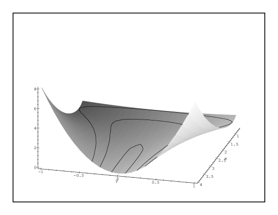
Figure 1: Hyperbolic wall potential

In figure (1) and (2) we present the form of the potential (4.24) and (2.13), respectively and draw corresponding equipotential lines. Simple calculations show that the maximum of $g$ is reached at the point $f=n/\sqrt{E}$. The minimal accessible value of $f$ is $f_{min}=n/\sqrt{2E}$. So, we deal with the potential for which equipotential lines go to infinity along the $f$-axis. Maximal value of $g/f$ in terms of $E,n$ and $\lambda$ is:

$$\zeta\equiv\left(\frac{g}{f}\right)_{max}=\frac{4\sqrt{2}}{3\sqrt{3}}\frac{E^{3/2}}{n^{2}\sqrt{\lambda}}$$ (4.29)

The condition $\zeta\ll 1$ guaranties that the system is always in the asymptotic region $g\sim\xi f$ with $\xi\ll 1$.

We integrate this system asymptotically by using Bogolyubov-Krylov method [19]. According to this method one has to take

$$g(t)=\sqrt{\frac{2\alpha}{\lambda f(t)}}\cos\varphi(t)$$ (4.30)

with some constant $\alpha$, then integrate the equation

$$\frac{d^{2}f}{dt^{2}}+\alpha-\frac{n^{2}}{f^{3}}=0$$ (4.31)

Equation (4.31) can be easily integrated,

$$t = \int\frac{df}{\sqrt{2\alpha(f_{max}-f)-\frac{n^{2}}{f^{2}f_{max}^{2}}(f_{max}^{2}-f^{2})}}$$ (4.32)

$$\varphi = \sqrt{\lambda}\int f(t)dt+\varphi_{0}$$ (4.33)

Here constant of integration is chosen so that at $t=0$ the $f$-coordinate takes its maximal value. Energy $E$ and maximal deviation $f_{max}$ are related as follows:

$$E=\alpha f_{max}+\frac{n^{2}}{2f_{max}^{2}}$$ (4.34)

One can invert this algebraic equation and get $f_{max}$ as function of dynamical variables of our system (4.24).

As result we suggest that in close analogy with previous model for $\zeta\ll 1$ the system becomes integrable and $f_{max}$ is integral of motion. We shall justify this conjecture numerically.

5 Numeric calculations.

In this section we investigate the existence of chaos-order transition for the hyperbolic model with reflecting wall, model with hyperbolic wall (4.24) and system (2.13) numerically.

At first we test the Poincarè sections for the model with a reflecting wall. The conservation of energy restricts any trajectory of the four-dimensional phase space to a three-dimensional energy shell. At a given energy any additional constraint defines a two-dimensional surface in the phase space, which is called the Poincarè section It is convenient to take a constraint $g=0$. All crossections of a trajectory with the surface are marked by points on the $(f,p_{f})$-plane. On each figure we plot a Poincarè section for a set of trajectories to show that behavior of the system does not depend on the initial data. Any trajectory was integrated as long as the program guarantees that the deviation of the energy is less then $0.1\%$. Different colors correspond to different trajectories with fixed parameters and random initial data. Chaotic motion is characterized by a set of randomly distributed points. Regular trajectories are depicted by dotted curves.

In Figures (3), (4) and (5) we plot Poincarè sections for the different values of the reflecting wall coordinate $l$ and with the same energy $E=1$. The pictures show that for small values of the parameter $l$ chaotic region is located near the wall. For large values of the parameter $l$ the points arrange into closed dotted curves.

An important characteristic of a dynamical system is the Lyapunov exponent $\eta(t)$. It has a positive limit: $(\lim_{t\to\infty}\eta>0)$ for a chaotic system and zero limit: $(\lim_{t\to\infty}\eta=0)$ for a regular one. The calculations for the model with the hyperbolic wall (4.24) were performed for different values of $\zeta$ (4.29). By changing the energy $E$ with $\lambda$ and $n$ being fixed. We vary the parameter $\zeta$. The program starts with random initial data with given energy. The program calculates the coordinates $f$ and $g$, the energy, $f_{max}$ and the Lyapunov exponent. Typical results for $\zeta=1$ and $\zeta\ll 1$ are shown on Figures (6) and (7) respectively. One can see that for $\zeta=1$ (Fig. 6, white curve) Lyapunov exponent has a positive limit. For $\zeta\ll 1$ the Lyapunov exponent goes to zero (Fig. 7, white curve). Parameter $f_{max}$ (blue curve) for small $\zeta$ does not change with the time. Energy (red line) shows that program works perfectly and energy does conserve through the whole calculation time. The numerical calculations show that for $\zeta=1$ the system (4.24) is stochastic and for $\zeta\ll 1$ it is the integrable one, that confirm the analytical results of sect. 4.

Now we turn to the main model (2.13). The dynamics of (2.13) was analyzed in [12] for relatively small (in units of $E$) values of $n$ and we have found it to be fully chaotic. For the relatively large values of $n$ the motion is confined into the region $\zeta\ll 1$ (see Fig. 2). In this region the model with hyperbolic wall (4.24) gives a good approximation to the main model (2.13). We conjecture the main model also to be integrable for the large $n$. In favor of this conjecture in Figures (8), (9) and (10) we plot the Poincarè sections for (2.13) with different values of parameter $n$ and fixed energy $E=1$. For large values of parameter $n$ there are only regular closed orbits. We also test the Lyapunov exponent and obtained the pictures quite similar to the ones for the model (4.24). Therefore we see that the system exhibit the chaos-order transition governed by the characteristic parameter $\zeta$.

 

ACKNOWLEDGMENT

 

The authors are grateful to B.V.Medvedev for stimulating discussions. I.A., P.M. and O.R. are supported in part by RFFI grant 96-01-00608. I.V. is supported in part by RFFI grant 96-01-00312. I.A. is supported in part by INTAS 96-0698.

 

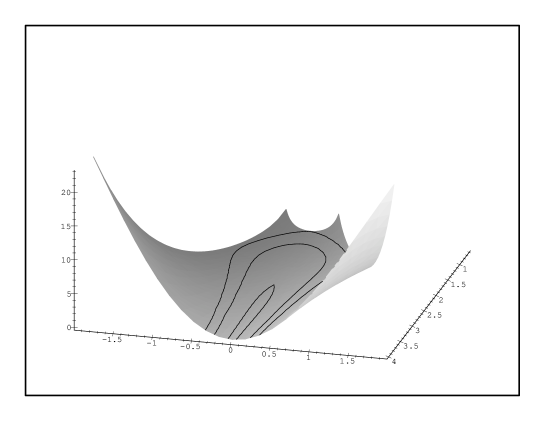
Figure 2: Full potential

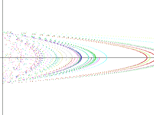
Figure 3: Reflecting wall potential, $l=1,~{}E=1$

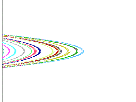
Figure 4: Reflecting wall potential, $l=10,~{}E=1$

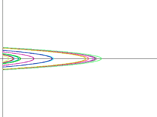
Figure 5: Reflecting wall potential, $l=50,~{}E=1$

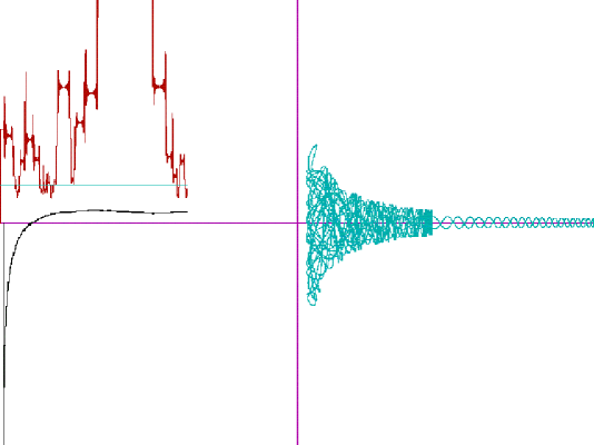
Figure 6: Chaotic phase

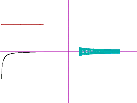
Figure 7: Regular phase

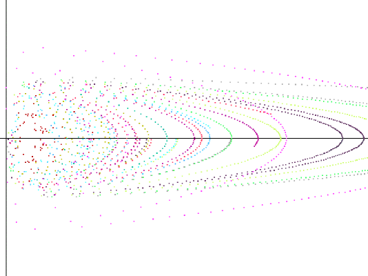
Figure 8: Full potential, $n=1,~{}e=1$

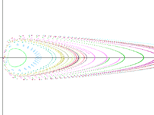
Figure 9: Full potential, $n=2,~{}e=1$

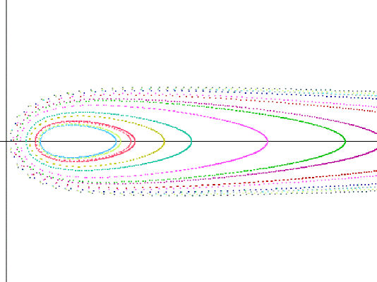
Figure 10: Full potential, $n=5,~{}e=1$

References

- [1] T. Banks, W. Fischler, S. H. Shenker and L. Susskind, M Theory as a Matrix Model: a Conjecture, Phys. Rev. D55(1997)5112, hep-th/9610043
- [2] B. de Wit, J. Hoppe and H. Nicolai, Nucl. Phys. B305 (1988) 545
- [3] B. de Wit, M.Luscher and H. Nicolai, Nucl. Phys. B 320 (1989) 135
- [4] J. Frhlich and J. Hoppe , On Zero-Mass Ground States in Super-Membrane Matrix Models, ITH-TH/96-53
- [5] E. Witten, Nucl. Phys. B443(1995)85
- [6] U. H. Danielsson, G. Ferretti and B. Sundborg, hep-th/9603081
- [7] D. Kabat and P. Pouliot, hep-th/9603127
- [8] L. Susskind, hep-th/9704080
- [9] T. Banks, hep-th/9710231
- [10] D.Bigatti and L.Susskind, hep-th/9712072
- [11] W. Taylor, hep-th/9801182
- [12] I.Ya. Arefe’eva, P.B. Medvedev, O.A. Rytchkov and I.V. Volovich, hep-th/9710032
- [13] I.Ya. Arefe’eva, G. Ferretti and A.S.Koshelev, hep-th/9804018
- [14] G. Z. Baseyan, S. G. Matinyan and G. K. Savvidi, JETP Lett. 29 (1979) 585
- [15] B. V. Chirikov and D. L. Shepelyanskii, JETP Lett. 34(1981)164
-
[16]
E.S. Nikolaevsky and L.N. Shchur,
JETP LEtt., 36 (1982) 218-220;
JETP 58 (1983) 1;
L. Salasnich, Mod. Phys. Lett. A12 (1997) 1473-1480, quant-ph/9706025;
J. D. Barrow and J. Levin, gr-qc/9706065; J. D. Barrow, M. P. Dabrowski, hep-th/9711041 - [17] L. Casetti, R. Gatto and M. Modugno, hep-th/9707054
- [18] B. V. Medvedev, Teor. Mat. Phys. 60(1984)224; 79(1989)404
- [19] N. N. Bogolyubov, Yu. A. Mitropolsky Asimptotics methods in the theory of non-linear oscillations. Physmathgiz, 1958 (in Russian).