hep-th/9804018
SISSA ref. 34/98/EP

Taming the Non Abelian Born-Infeld Action
Irina Ya. Aref’eva
Steklov Mathematical Institute, Russian Academy of Sciences

Gubkin St.8, GSP-1, 117966, Moscow, Russia

arefeva@mi.ras.ru,

Gabriele Ferretti
SISSA, Via Beirut 2 Trieste 34013, Italy

ferretti@sissa.it
and

Alexey S. Koshelev
Physical Department, Moscow State University,

Moscow, Russia, 119899

kas@depni.npi.msu.su

We show how to reduce the non abelian Born-Infeld action describing the interaction of two D-particles to the sum of elliptic integrals depending on simple kinematic invariants. This representation gives explicitly all $\alpha^{\prime}$ corrections to D-particle dynamics. The $\alpha^{\prime}$ corrections induce a stabilization of the classical trajectories such as the “eikonal” which are unstable within the Yang-Mills approximation.

1 Introduction

Since Dirichlet-branes (D-branes) found their true place in string theory [1], they have been challenging our basic intuitions about space-time. One of the most intriguing features is the fact that the coordinates describing the relative positions of D-branes naturally appear to be matrix valued [2], a fact that is at the heart of the matrix theory conjecture [3] (for a review see [4]).

In the matrix theory limit [5, 6], the form of the action relevant for the dynamics is simply the dimensionally reduced maximally supersymmetric Yang–Mills theory [7]- [13] but this is not so in other regimes. A specific example is ordinary weakly coupled type II (A or B) string theory at fixed value of $\alpha^{\prime}$, where the relevant effective action is the disk generating functional, already a highly non local object that is not known in closed form. If one restricts oneself further to considering the limit where the accelerations and higher time derivatives are small (keeping however the possibility of having relativistic velocities), the relevant action is the non abelian generalization of the Born–Infeld action (NBI) [14] to be described below. The full supersymmetric extension of such action is still out of reach, but for our purposes the bosonic action of [14] will suffice.

One of the hurdles in using the usual form of the NBI lagrangian is the presence of the symmetrized trace operator in front of the usual square root of the determinant. This is particularly disconcerting in the case of a D-particle, where one would like to use this lagrangian to investigate corrections to the scattering processes of [13] or to the canonical quantization of [11, 12].

In this paper we solve this problem by showing how, in the case of two D-particles, the NBI lagrangian can be recast in the form of an ordinary function of a small number of kinematic invariants. The functional dependence of the lagrangian on these invariants in through elliptic integrals.

As a first application of our result we investigate the stability of the eikonal trajectory, which is known to be unstable in the Yang–Mills system which is chaotic [24]. We show how the $\alpha^{\prime}$ corrections change the problem from the usual one of particles in flat space subjected to a quartic potential with flat directions to that of particles in conformally flat space with a similar potential. The curvature computed from the conformal factor is positive in the region near the flat directions thus contributing to the stabilization.

Two further issues that we leave for future work are the possibility of existence of trajectories other than the eikonal but with the same asymptotic behavior as $|t|\to\infty$. It would be interesting to find such trajectories where two D-particles come close, exchange their identity through a rotation in “non commutative space” and then separate again. Such trajectories do not exist in the truncated Yang–Mills theory [25] but may be present for the full NBI action. Another interesting issue would be to study the effects that the $\alpha^{\prime}$ corrections have on the Born–Oppenheimer approximation, perhaps suggesting a change of variables that makes it applicable for small distances.

The paper is organized as follows. In the next section we state Tseytlin’s result [14] on the form of the NBI action that is the starting point of our investigation. We also summarize the basic elementary features of the symmetric trace necessary to give a precise meaning to Tseytlin’s action. In section three we show how to rewrite the NBI action as a simple function of a few invariants in the case of two D-particles. We begin by stating the result and all the assumptions that go into it and end with the actual proof. The last section contains a first look at the dynamics that can be obtained from such an action (e.g. the stabilization of the eikonal) and some possible future directions to be explored.

2 The Non Abelian Born Infeld Action

Already at tree level in the string coupling $g_{s}$ (disk diagram) and in flat space-time $g_{\mu\nu}=\eta_{\mu\nu}={\rm diag}(-1,1,\cdots,1)$, the effective action for $N$ Dp-branes is a highly complicated object that is not known in closed form. This is of course due to the fact that, even at tree level, the n-point function on the disk receives contributions from the massive string states that, when integrated out, yield a non local functional of the massless modes.

If one makes the further approximation of neglecting higher derivatives of the field strength $F$ and, by consistency, terms involving the commutator of two field strengths as $[F,F]\equiv[D,D]F$, one can cast the bosonic part of the remaining action in the non abelian generalization of the Born Infeld action (NBI):

$$S=-\frac{1}{2g_{s}}\int dx^{p+1}\mathop{\rm Str}\nolimits\sqrt{-\det\bigg{(}\eta_{\mu\nu}+2\pi\alpha^{\prime}F_{\mu\nu}\bigg{)}},$$ (1)

where $\mu,\nu=0,\cdots,9$ but the field strength $F_{\mu\nu}$ only depends on the first $p+1$ coordinates (coordinates on the Dp-brane). The determinant $\det$ is taken only on the Lorentz indices $\mu$ and $\nu$ and the symmetric trace $\mathop{\rm Str}\nolimits$ will be discussed in more details below. Note that the determinant of a matrix with non commuting elements can be defined in many inequivalent ways; the symmetric trace $\mathop{\rm Str}\nolimits$ picks out the definition of physical interest.

2.1 The Symmetric Trace

The symmetric trace of a set of $n$ matrices is defined as the sum of the ordinary traces over all possible permutations $\pi\in S^{n}$ with the appropriate weight $1/n!$

$$\mathop{\rm Str}\nolimits(A_{1},\cdots,A_{n})=\frac{1}{n!}\sum_{\pi\in S^{n}}\mathop{\rm Tr}\nolimits(A_{\pi(1)}\cdots A_{\pi(n)}).$$ (2)

The trivial technical point that must be understood about the symmetric trace $\mathop{\rm Str}\nolimits$ is that, contrary to the more familiar trace operator, it does not allow one to perform the matrix algebra inside it. To give an explicit example, let $A$, $B$ and $C$ be three arbitrary matrices and let $D=AB$. Then, while obviously $\mathop{\rm Tr}\nolimits(ABC)=\mathop{\rm Tr}\nolimits(DC)$, one has from (2)

$$\mathop{\rm Str}\nolimits(A,B,C)=\frac{1}{2}\mathop{\rm Tr}\nolimits(ABC+ACB)\not=\mathop{\rm Str}\nolimits(D,C)=\mathop{\rm Tr}\nolimits(ABC).$$ (3)

That’s why, to avoid any confusion it is better to write $\mathop{\rm Str}\nolimits(A,B,C)$ instead of $\mathop{\rm Str}\nolimits(ABC)$. For an arbitrary function $f(A_{1},\cdots,A_{n})$ of $n$ matrices $A_{i}$, the symmetric trace (with respect to those matrices) is defined by first expanding $f$ as a Taylor series and then performing the symmetric trace on each monomial:

$$\mathop{\rm Str}\nolimits(f(A_{1},\cdots,A_{n}))=\sum_{k_{1}\cdots k_{n}}\frac{1}{k_{1}!\cdots k_{n}!}f^{(k_{1},\cdots,k_{n})}(0,\cdots,0)\mathop{\rm Str}\nolimits(A_{1}^{(k_{1})},\cdots,A_{n}^{(k_{n})}).$$ (4)

It is important to understand that the superscripts $(k_{i})$ inside the $\mathop{\rm Str}\nolimits$ operator simply mean that the matrix $A_{i}$ is repeated $k_{i}$ times in the list and do not represent a multiplication.

In the case of (1) by $\mathop{\rm Str}\nolimits$ we always refer to the symmetrized trace with respect to the form $F$.

3 NBI action of D-particles

In this section we derive the explicit expression (i.e. we perform the symmetric trace) for the NBI action of two D-particles in a particular gauge that although simplifies some of the computation, does not make us loose generality. Since the computations involved are rather laborious, we will begin by explaining the choice of gauge and stating the result; the remainder of the section deals only with the derivation of our expression for the NBI action.

3.1 Choice of gauge and statement of the result

Let us consider two D-particles moving in the $\hat{1},\;\hat{2}$ plane and let us set $A_{0}=A$, $A_{k}=X_{k}$ ($k=1,2$ only) so that

$$F_{0k}=\frac{d}{dt}X_{k}-i[A,X_{k}]\equiv DX_{k}\quad\hbox{and}\quad F_{12}=-i[X_{1},X_{2}]$$ (5)

where all fields are $SU(2)$ valued. While keeping track of the non abelian nature of the coordinates, one can still partially fix the gauge to be

$$X_{k}=x_{k}^{1}\sigma^{1}+x_{k}^{2}\sigma^{2},\quad\hbox{and}\quad A=a\sigma^{3}.$$ (6)

This gauge can be reached as follows: at each time $t$ one chooses the gauge transformation $g(t)$ that sets the commutator $[X_{1},X_{2}]$ proportional to $\sigma^{3}$. The remaining $U(1)$ gauge freedom of rotating along the $\sigma^{1},\sigma^{2}$ plane is compensated by the gauge field $A=a\sigma^{3}$. If the commutator is zero, the transformation above is ill defined, but in this case $X_{1}$ and $X_{2}$ are parallel in the $SU(2)$ Lie algebra and can both be made independent on $\sigma^{3}$ by a gauge rotation.

The main statement is that the NBI action in this gauge can be written in terms of the following three quantities, invariant in the unbroken gauge

$$\rho = 4(x_{1}^{1}x_{2}^{2}-x_{2}^{1}x_{1}^{2})^{2}$$

$$\eta = \frac{1}{2}\Big{(}(\dot{x}_{1}^{1})^{2}+(\dot{x}_{2}^{1})^{2}+(\dot{x}_{1}^{2})^{2}+(\dot{x}_{2}^{2})^{2}\Big{)}$$

$$-\frac{1}{2}\sqrt{\Big{(}(\dot{x}_{1}^{1})^{2}+(\dot{x}_{2}^{1})^{2}-(\dot{x}_{1}^{2})^{2}-(\dot{x}_{2}^{2})^{2}\Big{)}^{2}+4\Big{(}\dot{x}_{1}^{1}\dot{x}_{1}^{2}+\dot{x}_{2}^{1}\dot{x}_{2}^{2}\Big{)}^{2}}$$

$$\nu = \frac{1}{2}\Big{(}(\dot{x}_{1}^{1})^{2}+(\dot{x}_{2}^{1})^{2}+(\dot{x}_{1}^{2})^{2}+(\dot{x}_{2}^{2})^{2}\Big{)}$$ (7)

$$+\frac{1}{2}\sqrt{\Big{(}(\dot{x}_{1}^{1})^{2}+(\dot{x}_{2}^{1})^{2}-(\dot{x}_{1}^{2})^{2}-(\dot{x}_{2}^{2})^{2}\Big{)}^{2}+4\Big{(}\dot{x}_{1}^{1}\dot{x}_{1}^{2}+\dot{x}_{2}^{1}\dot{x}_{2}^{2}\Big{)}^{2}}$$

as

$$S(\rho,\eta,\nu) = -\sqrt{(1+\rho)\frac{1-\nu}{1-\eta}}-\frac{\nu}{\sqrt{\nu+\rho}}\Big{(}F(\phi,m)-F(\pi/2,m)\Big{)}$$ (8)

$$+\sqrt{\nu+\rho}\Big{(}E(\phi,m)-E(\pi/2,m)\Big{)}$$

where $F$ and $E$ are the elliptic integrals of first and second kind respectively whose arguments are:

$$\phi=\arcsin\sqrt{\frac{1-\nu}{1-\eta}}\quad\hbox{and}\quad m=\frac{\eta+\rho}{\nu+\rho}.$$ (9)

Since there are different conventions in the literature, let us also recall the definition of the elliptic integrals we are using:

$$F(\phi,m)=\int_{0}^{\phi}\;\frac{d\theta}{\sqrt{1-m\sin^{2}\theta}}\quad\hbox{and}\quad E(\phi,m)=\int_{0}^{\phi}\sqrt{1-m\sin^{2}\theta}\;d\theta.$$ (10)

$F(\pi/2,m)$ and $E(\pi/2,m)$ are known as complete elliptic integrals and are sometimes indicated by $K(m)$ and $E(m)$.

For completeness, let us write the action of $R$, the generator of rotation in the $\hat{1},\;\hat{2}$ plane, and $G$, the generator of the left over $U(1)$ gauge invariance.

$$R:\left\{\begin{array}[]{c}\pmatrix{x_{1}^{1}\cr x_{2}^{1}\cr}\rightarrow\pmatrix{\tilde{x}_{1}^{1}\cr\tilde{x}_{2}^{1}\cr}=\pmatrix{\cos\theta x_{1}^{1}-\sin\theta x_{2}^{1}\cr\sin\theta x_{1}^{1}+\cos\theta x_{2}^{1}\cr}\\ \\ \pmatrix{x_{1}^{2}\cr x_{2}^{2}\cr}\rightarrow\pmatrix{\tilde{x}_{1}^{2}\cr\tilde{x}_{2}^{2}\cr}=\pmatrix{\cos\theta x_{1}^{2}-\sin\theta x_{2}^{2}\cr\sin\theta x_{1}^{2}+\cos\theta x_{2}^{2}\cr}\end{array}\right.$$

$$G:\left\{\begin{array}[]{c}\pmatrix{x_{1}^{1}\cr x_{1}^{2}\cr}\rightarrow\pmatrix{\hat{x}_{1}^{1}\cr\hat{x}_{1}^{2}\cr}=\pmatrix{\cos\alpha(t)x_{1}^{1}-\sin\alpha(t)x_{1}^{2}\cr\sin\alpha(t)x_{1}^{1}+\cos\alpha(t)x_{1}^{2}\cr}\\ \\ \pmatrix{x_{2}^{1}\cr x_{2}^{2}\cr}\rightarrow\pmatrix{\hat{x}_{2}^{1}\cr\hat{x}_{2}^{2}\cr}=\pmatrix{\cos\alpha(t)x_{2}^{1}-\sin\alpha(t)x_{2}^{2}\cr\sin\alpha(t)x_{2}^{1}+\cos\alpha(t)x_{2}^{2}\cr}\\ \\ a\rightarrow\hat{a}=a-\frac{1}{2}\frac{d\alpha}{dt}\end{array}\right.$$

It is an easy matter to check that (7) are invariant under $R$ and $G$.

3.2 Derivation of the form of the action

The remainder if this section contains the derivation of (8).

We begin by evaluating the determinant in (1) without performing the matrix algebra:

$$\det(\eta_{\mu\nu}+F_{\mu\nu})=\det\pmatrix{-1&DX_{1}&DX_{2}\cr-DX_{1}&1&-i[X_{1},X_{2}]\cr-DX_{2}&i[X_{1},X_{2}]&1\cr}$$

$$=-1+(DX_{1},-DX_{2},-i[X_{1},X_{2}])+(-DX_{1},DX_{2},i[X_{1},X_{2}])$$

$$-(1,DX_{2},-DX_{2})-(1,DX_{1},-DX_{1})-(-1,i[X_{1},X_{2}],-i[X_{1},X_{2}])$$

$$=-1+(DX_{k},DX_{k})+([X_{1},X_{2}],[X_{1},X_{2}])$$ (11)

where the last simplification is allowed because all these terms will be used inside the symmetric trace. By expanding the square root as a double power series one gets

$$S = -\frac{1}{2}\mathop{\rm Str}\nolimits\sqrt{-\det(\eta_{\mu\nu}+F_{\mu\nu})}$$

$$= -\frac{1}{2}\mathop{\rm Str}\nolimits\sqrt{1-(DX_{k},DX_{k})-([X_{1},X_{2}],[X_{1},X_{2}])}$$

$$= \sum_{m,q=0}^{\infty}\frac{1}{2^{2m+2q}}\frac{(2m+2q-2)!}{m!q!(m+q-1)!}\mathop{\rm Str}\nolimits(DX_{k}^{(2m)},[X_{1},X_{2}]^{(2q)}),$$

where, for $m=q=0$ we define the coefficient of the symmetric trace to be equal to its “analytically continued” value $-1/2$.

Eq. (LABEL:NBIpart) can be simplified by noticing that the commutator $[X_{1},X_{2}]$ anti-commutes with the covariant derivatives and has square proportional to the identity matrix. This allows one to write

$$\mathop{\rm Str}\nolimits(DX_{i}^{(2m)},[X_{1},X_{2}]^{(2q)})=\frac{2m!2q!}{(2q+2m)!}\frac{(m+q)!}{m!q!}(-1)^{q}\rho^{q}\mathop{\rm Str}\nolimits(DX_{i}^{(2m)})$$ (13)

in terms of the invariant $\rho$ defined in (7). Note that we are still using $\mathop{\rm Str}\nolimits$.

The reader can check the validity of (13) by chosing the term in the sum containing only $DX_{1}$, expanding the symmetric trace into $(2m+2q)!$ ordinary traces according to (2) and grouping the $2m!2q!$ identical terms coming from the permutations of $DX_{1}$ with themselves and $[X_{1},X_{2}]$ with themselves. In each of the remaining $(2m+2q)!/2m!2q!$ terms one then brings all the commutators $[X_{1},X_{2}]$ to the left keeping track of the signs. There is an excess of $(m+q)!/m!q!$ terms with positive sign, yielding

$$\mathop{\rm Str}\nolimits(DX_{1}^{(2m)},[X_{1},X_{2}]^{(2q)})=\frac{2m!2q!}{(2q+2m)!}\frac{(m+q)!}{m!q!}(-1)^{q}\rho^{q}\mathop{\rm Tr}\nolimits(DX_{1}^{2m}).$$ (14)

Eq. (13) follows by replacing $(DX_{1})^{(2)}$ by $(DX_{i})^{(2)}$ and $\mathop{\rm Tr}\nolimits$ by $\mathop{\rm Str}\nolimits$ on the r.h.s. of (14).

With this simplification:

$$S=\sum_{m,q=0}^{\infty}\frac{1}{2^{2m+2q+1}}\frac{2m!2q!}{m!^{2}q!^{2}}\frac{(-1)^{q}}{2q+2m-1}\rho^{q}\mathop{\rm Str}\nolimits(DX_{i}^{(2m)}).$$ (15)

To proceed further, define three (non invariant) intermediate quantities

$$a=(\dot{x}_{1}^{1})^{2}+(\dot{x}_{2}^{1})^{2}$$

$$b=2(\dot{x}_{1}^{1}\dot{x}_{1}^{2}+\dot{x}_{2}^{1}\dot{x}_{2}^{2})$$

$$c=(\dot{x}_{1}^{2})^{2}+(\dot{x}_{2}^{2})^{2}$$ (16)

and carefully expand the symmetric trace using (2)

$$\mathop{\rm Str}\nolimits(DX_{i}^{(2m)})=\mathop{\rm Str}\nolimits\bigg{(}\Big{(}(\dot{x}_{1}^{1}\sigma^{1}+\dot{x}_{1}^{2}\sigma^{2})^{(2)}+(\dot{x}_{2}^{1}\sigma^{1}+\dot{x}_{2}^{2}\sigma^{2})^{(2)}\Big{)}^{(m)}\bigg{)}$$

$$=\mathop{\rm Str}\nolimits\bigg{(}\Big{(}a(\sigma^{1},\sigma^{1})+b(\sigma^{1},\sigma^{2})+c(\sigma^{2},\sigma^{2})\Big{)}^{(m)}\bigg{)}$$

$$=\sum_{i+j+k=m}\frac{m!}{i!j!k!}a^{i}b^{j}c^{k}\mathop{\rm Str}\nolimits\Big{(}(\sigma^{1})^{(2i+j)}(\sigma^{2})^{(2k+j)}\Big{)}$$

$$=\sum_{i+j+k=m}2\frac{m!^{2}}{2m!}\frac{a^{i}b^{j}c^{k}}{i!j!k!}\left(\frac{1+(-1)^{j}}{2}\right)\frac{(2i+j)!(2k+j)!}{(i+j/2)!(k+j/2)!}.$$ (17)

The reason for the combinatorics in the last line of (17) is exactly the same as the one given for (13); also note that the symmetric trace vanishes for $j$ odd explaining the presence of the projection operator $(1+(-1)^{j})/2$ and term of the type $j/2$ in the factorial. In fact, by using the identity

$$\sum_{m=0}^{\infty}\sum_{i+j+k=m}a_{m,i,j,k}=\sum_{i,j,m=0}^{\infty}a_{m+i+j,i,j,m}$$ (18)

and replacing $j$ by $2j$, we have the following multiple power series for the NBI action:

$$S=\sum_{q,m,i,j=0}^{\infty}\frac{(-1)^{q}}{2^{2m+2i+4j+2q}}\frac{2q!}{q!^{2}}\frac{(2i+2j)!(2m+2j)!}{i!2j!m!(i+j)!(m+j)!}\frac{\rho^{q}a^{i}b^{2j}c^{m}}{2m+2i+4j+2q-1}.$$ (19)

To simplify things slightly, let us introduce four new variables $x,y,z,w$ and define

$$U(x,y,z,w)=\sum_{q,m,i,j=0}^{\infty}\frac{2q!}{q!^{2}}\frac{(2i+2j)!(2m+2j)!}{i!2j!m!(i+j)!(m+j)!}\frac{x^{2m}y^{2i}z^{4j}w^{2q}}{2m+2i+4j+2q-1}$$ (20)

Trivially, if one knows $U$, the NBI action is

$$S=U(\sqrt{c}/2,\sqrt{a}/2,\sqrt{b}/2,i\sqrt{\rho}/2).$$ (21)

To obtain a closed expression for $U$ notice that there is a very similar expression that can be easily summed:

$$Z(x,y,z,w)=\sum_{q,m,i,j=0}^{\infty}\frac{2q!}{q!^{2}}\frac{(2i+2j)!(2m+2j)!}{i!2j!m!(i+j)!(m+j)!}x^{2m}y^{2i}z^{4j}w^{2q}$$

$$=\frac{1}{\sqrt{(1-4w^{2})\Big{(}(1-4x^{2})(1-4y^{2})-4z^{4}\Big{)}}}.$$ (22)

The functions $U$ and $Z$ are related by the PDE:

$$\Big{(}x\partial_{x}+y\partial_{y}+z\partial_{z}+w\partial_{w}-1\Big{)}U=Z$$ (23)

and we are left with the problem of finding the solution to (23) compatible with the conditions given by the power series (20). Let us first find the most general solution to (23) by making the change of variable

$$p=(xyzw)^{1/4},\quad r=\left(\frac{w}{x}\right)^{1/4},\quad q=\left(\frac{w}{y}\right)^{1/4}\quad s=\left(\frac{w}{z}\right)^{1/4}$$ (24)

that reduces the PDE to an ODE

$$\Big{(}p\partial_{p}-1\Big{)}U=Z$$ (25)

whose most general solution in terms of an arbitrary function $g(r,q,s)$ is

$$U=p\left(g(r,q,s)+\int^{p}\frac{Z}{p^{2}}\;dp\right).$$ (26)

Performing the elliptic integral we obtain

$$U = pg(r,q,s)-\sqrt{\frac{1-2\Big{(}x^{2}+y^{2}+\sqrt{(x^{2}-y^{2})^{2}+z^{4}}\Big{)}}{1-2\Big{(}x^{2}+y^{2}-\sqrt{(x^{2}-y^{2})^{2}+z^{4}}\Big{)}}(1-4w^{4})}$$ (27)

$$-\frac{2\Big{(}x^{2}+y^{2}+\sqrt{(x^{2}-y^{2})^{2}+z^{4}}\Big{)}}{\sqrt{2\Big{(}x^{2}+y^{2}+\sqrt{(x^{2}-y^{2})^{2}+z^{4}}\Big{)}-4w^{2}}}\;F(\phi,m)$$

$$+\sqrt{2\Big{(}x^{2}+y^{2}+\sqrt{(x^{2}-y^{2})^{2}+z^{4}}\Big{)}-4w^{2}}\;E(\phi,m)$$

with

$$\phi = \arcsin\sqrt{\frac{1-2\Big{(}x^{2}+y^{2}+\sqrt{(x^{2}-y^{2})^{2}+z^{4}}\Big{)}}{1-2\Big{(}x^{2}+y^{2}-\sqrt{(x^{2}-y^{2})^{2}+z^{4}}\Big{)}}}$$

$$m = \frac{2\Big{(}x^{2}+y^{2}-\sqrt{(x^{2}-y^{2})^{2}+z^{4}}\Big{)}-4w^{2}}{2\Big{(}x^{2}+y^{2}+\sqrt{(x^{2}-y^{2})^{2}+z^{4}}\Big{)}-4w^{2}}.$$ (28)

The function $g(r,q,s)$ can be fixed by imposing that the solution should not have any term linear in $x,y,z,w$ in its power series around the origin. Hence, by computing $U$ along the line $x=t/r^{4},\;y=t/q^{4},\;z=t/s^{4},\;w=t$ and imposing the vanishing of the $O(t)$ terms one obtains

$$pg(r,q,s) = \frac{2\Big{(}x^{2}+y^{2}+\sqrt{(x^{2}-y^{2})^{2}+z^{4}}\Big{)}}{\sqrt{2\Big{(}x^{2}+y^{2}+\sqrt{(x^{2}-y^{2})^{2}+z^{4}}\Big{)}-4w^{2}}}\;F(\pi/2,m)$$ (29)

$$-\sqrt{2\Big{(}x^{2}+y^{2}+\sqrt{(x^{2}-y^{2})^{2}+z^{4}}\Big{)}-4w^{2}}\;E(\pi/2,m).$$

Tracing back the various changes of variables to (7) (c.f.r. also (16) and (21) we obtain our final answer (8). Note that the three non invariant quantities $a$, $b$ an $c$ have combined into two invariants $\nu$ and $\eta$ ($\rho$ was invariant from the beginning) so that the final expression (8) is depending only on the three variables (7) and not four.

4 Some simple properties of the action

To get a first feeling for the quantities $\rho$, $\eta$ and $\nu$, note that, in the commuting limit $\rho=\eta=0$ and $\nu=v^{2}$, $v$ being the relative velocity of the two D-particles. Substituting these values into (8), one finds the expected result

$$S=-\sqrt{1-\nu}=-\sqrt{1-v^{2}}.$$ (30)

Another trivial limit is that where all time dependence is dropped, i.e. $\eta=\nu=0$, $\rho=-\mathop{\rm Tr}\nolimits([X_{1},X_{2}]^{2})$ where one finds the potential

$$S=-\sqrt{1+\rho}=-\frac{1}{2}\mathop{\rm Tr}\nolimits\sqrt{1-[X_{1},X_{2}]^{2}}.$$ (31)

With the proper factors of the string slope reinstated, to leading order in $\alpha^{\prime}$ (31) is simply the Yang-Mills potential and $\rho$ measures the distance from the bottom of the valley.

A less trivial limit comes by asking what is the form of the kinetic term exact to all orders in $\alpha^{\prime}$. Here one already encounters an expression that could not have been guessed simply from (1). Although it is possible to obtain this from the full answer (8), we find it easier to go back to the partial sum (15) and specialize to the $m=1$ case. The coefficient of

$$\mathop{\rm Str}\nolimits(DX_{i}^{(2)})\equiv\mathop{\rm Tr}\nolimits(DX_{i}^{2})=2\Big{(}(\dot{x}_{1}^{1})^{2}+(\dot{x}_{2}^{1})^{2}+(\dot{x}_{1}^{2})^{2}+(\dot{x}_{2}^{2})^{2}\Big{)}$$ (32)

is

$$f_{1}(\rho)=\sum_{q=0}^{\infty}\frac{1}{2^{2q+2}}\frac{2q!}{q!^{2}}\frac{(-1)^{q}}{2q+1}\rho^{q}=\frac{\mathop{\rm arcsinh}\nolimits(\sqrt{\rho})}{4\sqrt{\rho}}.$$ (33)

Thus, for small velocities but to all orders in $\alpha^{\prime}$, the lagrangian governing the dynamics of two D-particles in this gauge is given by

$${\cal L} = \frac{\mathop{\rm arcsinh}\nolimits\bigg{(}2(x_{1}^{1}x_{2}^{2}-x_{2}^{1}x_{1}^{2})\bigg{)}}{4(x_{1}^{1}x_{2}^{2}-x_{2}^{1}x_{1}^{2})}\bigg{(}(\dot{x}_{1}^{1})^{2}+(\dot{x}_{2}^{1})^{2}+(\dot{x}_{1}^{2})^{2}+(\dot{x}_{2}^{2})^{2}\bigg{)}$$ (34)

$$-\sqrt{1+4(x_{1}^{1}x_{2}^{2}-x_{2}^{1}x_{1}^{2})^{2}}.$$

Eq. (34) describes the motion in a conformally flat space.

It is possible to use the same change of variables introduced in  [24] to eliminate two of the four variables in (34) by virtue of the symmetries $R$ and $G$. Setting

$$x_{1}^{1} = f\cos\theta\cos\phi-g\sin\theta\sin\phi$$

$$x_{1}^{2} = -f\cos\theta\sin\phi-g\sin\theta\cos\phi$$

$$x_{2}^{1} = f\sin\theta\cos\phi+g\cos\theta\sin\phi$$

$$x_{2}^{2} = -f\sin\theta\sin\phi+g\cos\theta\cos\phi$$ (35)

and eliminating the cyclic coordinates $\theta$ and $\phi$ through their equations of motion

$$(f^{2}+g^{2})\dot{\phi}+2fg\dot{\theta} = 0$$

$$2fg\dot{\phi}+(f^{2}+g^{2})\dot{\theta} = l\frac{2fg}{\mathop{\rm arcsinh}\nolimits(2fg)}$$ (36)

one obtains the Routhian (still denoted by ${\cal L}$)

$${\cal L}=\frac{1}{2}K\left(\dot{f}^{2}+\dot{g}^{2}\right)-V,$$ (37)

where

$$K=\frac{\mathop{\rm arcsinh}\nolimits(2fg)}{2fg}\quad\hbox{and}\quad V=\frac{l^{2}}{K^{2}}\frac{f^{2}+g^{2}}{(f^{2}-g^{2})^{2}}+\sqrt{1+4f^{2}g^{2}}.$$ (38)

In these coordinates the eikonal takes the form

$$g=0,\quad\phi=0,\quad f=\sqrt{v^{2}t^{2}+b^{2}},\quad\theta=\arctan(vt/b),$$ (39)

where $v$ and $b$ are the relative velocity and impact parameter respectively.

It is interesting to compute the curvature associated to the conformal factor $K$. This is partly because a previous analysis  [24] has shown that the eikonal trajectories are in fact unstable in the Yang–Mills case, the system being chaotic. A positive curvature would have a stabilizing effect on the classical trajectories. The Gauss curvature coming from the conformal factor $K$ turns out to be

$$R=-2(f^{2}+g^{2})\frac{(\log K)^{\prime\prime}}{K},$$ (40)

and it is indeed positive near the eikonal, thus having a balancing effect on the small fluctuations around it.

To study the balancing effect we analyze the system (37) numerically using Poincaré sections. The Poincaré section is a surface in phase space. Our phase space is four dimensional but energy conservation restricts the motion to be on a three dimensional subspace. One can then impose any constraint and fix a two dimensional surface named Poincaré section. We use the constraint $g=0$. A point is plotted each time the trajectory goes through the surface. A chaotic distribution of points says that the system under consideration is chaotic. If there are solid or dotted lines on the Poinacré section the system is regular.

We perform about 1000 experiments for 10 different values of the energy. We plot the typical Poincaré sections to show an appearance of the regular motion. Figures 1 and 2 show the Poincaré sections for trajectories started at point $f=5,g=0$ and $f=5$, $g=0.01$, respectively. Comparing these figures we see that the eikonal trajectory is stable. Figures 3 and 4 represent stochastic behavior of trajectories with the initial coordinates $f=5$, $g=0.1$ and $f=5$, $g=0.2$, respectively. All trajectories above have zero initial velocities. Figures 5 and 6 show the motion of the particle with initial conditions $f=10,$ $g=0.01$, $\dot{f}=-1$ and $f=20,$ $g=0.001$, $\dot{f}=-1$. One can see that the particle reaches a point of minimal $f$, ”scatters” and turns back without stochastization.

It would be interesting to pursue the study of (8) or some of its simplified limits like (37) further, in particular addressing some of the issues raised in the introduction such as the detail study of trajectories that resemble the eikonal only for $|t|\to\infty$ or ways of improving on the Born-Oppenheimer approximation near $\rho=0$, interesting for the study of Matrix black holes  [26]-[28].

5 Acknowledgments

We would like U. Danielsson, R. Iengo, J. Kalkkinen, P.B.Medvedev, O.A. Rytchkov, A. Schwimmer, and I.V. Volovich for discussions. I.A. and A.K. are supported by RFFI grant 96-01-00608, I.A. is supported by INTAS grant 96-

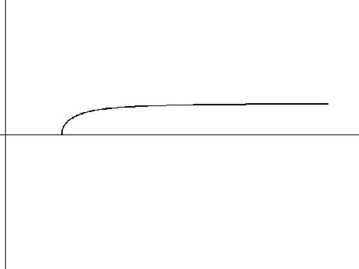
Figure 1: Poincaré section for trajectory with initial data $f=5,g=0$.

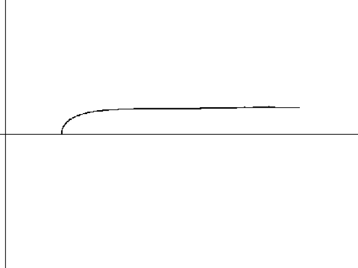
Figure 2: Poincaré section for trajectory with initial data $f=5,g=0.01$.

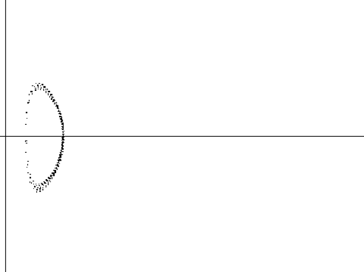
Figure 3: Poincaré section for trajectory with initial data $f=5,g=0.1$.

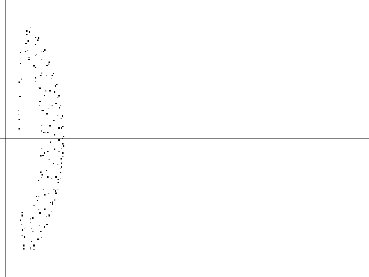
Figure 4: Poincaré section for trajectory with initial data $f=5,g=0.2$.

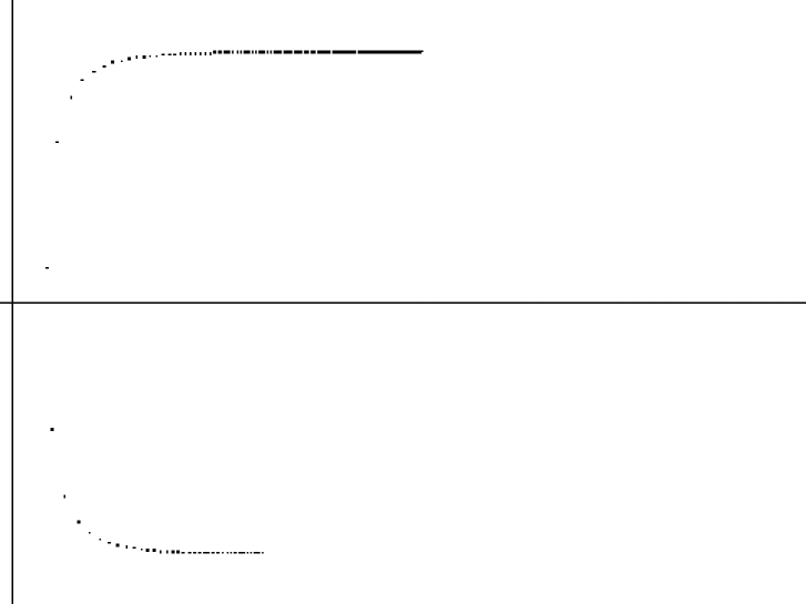
Figure 5: Poincaré section for trajectory with initial data $f=10,g=0.01$ and $\dot{f}=-1$.

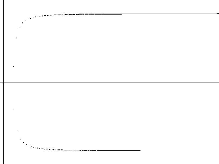
Figure 6: Poincaré section for trajectory with initial data $f=20,g=0.001$ and $\dot{f}=-1$.

References

• [1] J. Polchinski, Phys. Rev. Lett. 75 (1995) 4724, hep-th/9510017.
• [2] E. Witten, Nucl. Phys. B460 (1996) 335, hep-th/9510135.
• [3] T. Banks, W. Fischler, S.H. Shenker and L. Susskind, Phys. Rev. D55 (1997) 5112, hep-th/9610043.
• [4] T.Banks, hep-th/9710231
D.Bigatti and L.Susskind, hep-th/9712072
W.Taylor, hep-th/9801182
• [5] A. Sen, hep-th/9709220.
• [6] N. Seiberg, Phys. Rev. Lett. 79 (1997) 3577, hep-th/9710009.
• [7] M. Claudson and M.B. Halpern, Nucl. Phys. B25 (1985) 689.
• [8] M. Baake, P. Reinicke and V. Rittenberg, J. Math. Phys. 26 (1985) 1070.
• [9] R. Flume, Ann. Phys. 164 (1985) 189.
• [10] B. de Wit, J. Hoppe and H. Nicolai, Nucl. Phys. B305 (1988) 545.
• [11] U.H. Danielsson, G. Ferretti and B. Sundborg, Int. J. Mod. Phys. A11 (1996) 5463, hep-th/9603081.
• [12] D. Kabat and P. Pouliot, Phys. Rev. Lett. 77 (1996) 1004, hep-th/9603127.
• [13] M.R. Douglas, D. Kabat, P. Pouliot and S.H. Shenker, Nucl. Phys. B485 (1997) 85, hep-th/9608024.
• [14] A.A. Tseytlin, Nucl. Phys. B501 (1997) 41, hep-th/9701125
• [15] A. Neveu and J. Scherk, Nucl. Phys. B36 (1972) 155.
• [16] J. Scherk and J.H. Schwarz, Nucl. Phys. B81 (1974) 118.
• [17] E.S. Fradkin and A.A. Tseytlin, Phys. Lett. B163 (1985) 123.
• [18] D. Gross and E. Witten, Nucl. Phys. B277 (1986) 1.
• [19] A.A. Tseytlin, Nucl. Phys. B276 (1986) 391; Errata: Nucl. Phys. B291 (1987) 876.
• [20] A.A. Abouelsaood et al., Nucl. Phys. B280 (1987) 599.
• [21] E. Bergshoeff et al., Phys. Lett B188 (1987) 70.
• [22] R.R. Metsaev, M.A. Rahmanov and A.A. Tseytlin, Phys. Lett. B193 (1987) 207.
• [23] A.A. Tseytlin, Phys. Lett. B202 (1988) 81.
• [24] I.Ya. Aref’eva, P.M. Medvedev, O.A. Rytchkov and I.V. Volovich. hep-th/9710032, I.Ya. Aref’eva, A.S. Koshelev and P.M. Medvedev, in preparation.
• [25] I.Ya. Aref’eva, G. Ferretti, J. Kalkkinen, P.M. Medvedev and O.A. Rytchkov, unpublished.
• [26] M. Li and E. Martinec, Class. Quant. Grav. 14 (1997) 3187, hep-th/9703211.
• [27] H. Liu and A.A. Tseytlin, JHEP 01(1998)010, hep-th/9712063.
• [28] M. Li and E. Martinec, hep-th/9801070.
Refer to caption