Exactly solvable dynamical systems in
Oliver Haschke and Werner Rühl
Department of Physics, University of Kaiserslautern, P.O.Box 3049
67653 Kaiserslautern, Germany
Abstract
The Hamiltonian of the N 𝑁 N N = 3 𝑁 3 N=3 N = 4 𝑁 4 N=4 N 𝑁 N
April 1998
1 Introduction: The Calogero model
The Calogero model [1 ] is a quantum mechanical system of N 𝑁 N [2 ] . In [3 ] it has been shown that it can be
reduced to a representation theory problem of Lie algebras, so that both eigenvalues and
eigenfunctions can be extracted from finite dimensional representations of these algebras.
The idea that exact solvability and Lie algebraic representation might be connected was
presented in [4 ] , which dealt with exactly and quasiexactly solvable elementary models. Their
Hamiltonians were rewritten as quadratic polynomials in Lie algebra differential operators.
In this article it was also discussed first whether this procedure could be inverted: Find new
exactly solvable models from Lie algebras of differential operators. Usually this leads to
kinetic energy terms which are Laplace-Beltrami operators on a curved space. So the task arises
to construct quadratic polynomials from the Lie algebras with the constraint that the curvature
tensor vanishes identically on some dynamically accessible domain (”flat quadratic Lie algebraic forms”).
In order to maintain the notion of exact integrability, however, the nontrivial but curvature-free
Laplace-Beltrami operator should be transformed into a standard Laplace operator by an
explicitly known diffeomorphism. This has to be found from nonlinear partial differential
equations. In the neighborhood of the Calogero models for N = 3 𝑁 3 N=3 N = 4 𝑁 4 N=4 s 𝑠 s s = 0 𝑠 0 s=0
In the last year two further articles have appeared dealing with the algebraization of
solvable models [5 , 6 ] . We hope that these results can be used to simplify the inverse
issue, the construction of new solvable dynamical models.
Let us now outline the algebraization of the standard (sl(N)) Calogero model, since we use
it in the sequel. The Hamiltonian is
H = + 1 2 [ − Δ + ω 2 x 2 ] + ∑ i < j g ( x i − x j ) 2 𝐻 1 2 delimited-[] Δ superscript 𝜔 2 superscript 𝑥 2 subscript 𝑖 𝑗 𝑔 superscript subscript 𝑥 𝑖 subscript 𝑥 𝑗 2 H=+\frac{1}{2}[-\Delta+\omega^{2}x^{2}]+\sum_{i<j}\frac{g}{(x_{i}-x_{j})^{2}} (1.1)
where x ∈ I R N 𝑥 I subscript R 𝑁 x\in{\rm I\!R}_{N}
x 2 = ∑ i = 1 N x i 2 superscript 𝑥 2 subscript superscript 𝑁 𝑖 1 subscript superscript 𝑥 2 𝑖 x^{2}=\sum^{N}_{i=1}x^{2}_{i} (1.2)
g 𝑔 g
g = ν ( ν − 1 ) ≥ − 1 4 𝑔 𝜈 𝜈 1 1 4 g=\nu(\nu-1)\geq-\frac{1}{4} (1.3)
so that
ν = 1 2 ± ( g + 1 4 ) 1 2 𝜈 plus-or-minus 1 2 superscript 𝑔 1 4 1 2 \nu=\frac{1}{2}\pm(g+\frac{1}{4})^{\frac{1}{2}}
is an integer. If ν 𝜈 \nu
We factorize the solutions as
ψ ( x ) = V ( x ) ν e − 1 2 ω x 2 P ( x ) 𝜓 𝑥 𝑉 superscript 𝑥 𝜈 superscript 𝑒 1 2 𝜔 superscript 𝑥 2 𝑃 𝑥 \psi(x)=V(x)^{\nu}e^{-\frac{1}{2}\omega x^{2}}P(x) (1.4)
where V ( x ) 𝑉 𝑥 V(x)
V ( x ) = ∏ i < j ( x i − x j ) 𝑉 𝑥 subscript product 𝑖 𝑗 subscript 𝑥 𝑖 subscript 𝑥 𝑗 V(x)=\prod_{i<j}(x_{i}-x_{j}) (1.5)
and P ( x ) 𝑃 𝑥 P(x) { x i } 1 N subscript superscript subscript 𝑥 𝑖 𝑁 1 \{x_{i}\}^{N}_{1} ψ 𝜓 \psi
H ψ = E ψ 𝐻 𝜓 𝐸 𝜓 H\psi=E\psi (1.6)
then P 𝑃 P
h P = ϵ P ℎ 𝑃 italic-ϵ 𝑃 hP=\epsilon P (1.7)
with
h = − Δ + 2 ω ∑ i = 1 N x i ∂ ∂ x i − ν ∑ i ≠ j 1 x i − x j ( ∂ ∂ x i − ∂ ∂ x j ) ℎ Δ 2 𝜔 subscript superscript 𝑁 𝑖 1 subscript 𝑥 𝑖 subscript 𝑥 𝑖 𝜈 subscript 𝑖 𝑗 1 subscript 𝑥 𝑖 subscript 𝑥 𝑗 subscript 𝑥 𝑖 subscript 𝑥 𝑗 h=-\Delta+2\omega\sum^{N}_{i=1}x_{i}\frac{\partial}{\partial x_{i}}-\nu\sum_{i\not=j}\frac{1}{x_{i}-x_{j}}\left(\frac{\partial}{\partial x_{i}}-\frac{\partial}{\partial x_{j}}\right) (1.8)
and
ϵ = 2 E − N ω − ν N ( N − 1 ) ω italic-ϵ 2 𝐸 𝑁 𝜔 𝜈 𝑁 𝑁 1 𝜔 \epsilon=2E-N\omega-\nu N(N-1)\omega (1.9)
Next we introduce elementary symmetric functions (following [3 ] )
∏ i = 1 N ( 1 + x i t ) = ∑ n = 0 N σ n ( x ) t n ( σ 0 = 1 ) subscript superscript product 𝑁 𝑖 1 1 subscript 𝑥 𝑖 𝑡 subscript superscript 𝑁 𝑛 0 subscript 𝜎 𝑛 𝑥 superscript 𝑡 𝑛 subscript 𝜎 0 1 \prod^{N}_{i=1}(1+x_{i}t)=\sum^{N}_{n=0}\sigma_{n}(x)t^{n}\,(\sigma_{0}=1) (1.10)
For each element g ∈ S N 𝑔 subscript 𝑆 𝑁 g\in S_{N} N 𝑁 N
E g = { x i 1 < x i 2 < x i 3 < … < x i N ; \displaystyle E_{g}=\Big{\{}x_{i_{1}}<x_{i_{2}}<x_{i_{3}}<\ldots<x_{i_{N}};
( 1 , 2 , 3 , … N ) → g ( i 1 , i 2 , … i N ) } \displaystyle(1,2,3,\ldots N)\begin{array}[]{c}\\
\to\\
g\end{array}(i_{1},i_{2},\ldots i_{N})\Big{\}} (1.14)
⊂ I R N absent I subscript R 𝑁 \displaystyle\subset{\rm I\!R}_{N}\quad\quad\quad\quad (1.15)
so that the map
σ : x → { σ n } n = 1 N : 𝜎 → 𝑥 subscript superscript subscript 𝜎 𝑛 𝑁 𝑛 1 \sigma:x\to\{\sigma_{n}\}^{N}_{n=1} (1.16)
is a diffeomorphism. This follows from the fact that the Jacobian
ℳ a i = ∂ σ a ∂ x i subscript ℳ 𝑎 𝑖 subscript 𝜎 𝑎 subscript 𝑥 𝑖 {\cal M}_{ai}=\frac{\partial\sigma_{a}}{\partial x_{i}} (1.17)
has
det ℳ = V ( x ) ( − 1 ) [ N 2 ] ℳ 𝑉 𝑥 superscript 1 delimited-[] 𝑁 2 \det{\cal M}=V(x)(-1)^{[\frac{N}{2}]} (1.18)
where V ( x ) 𝑉 𝑥 V(x) v ( σ 1 , … , σ N ) 𝑣 subscript 𝜎 1 … subscript 𝜎 𝑁 v(\sigma_{1},\ldots,\sigma_{N}) D + ⊂ I R N subscript 𝐷 I subscript R 𝑁 D_{+}\subset{\rm I\!R}_{N} v > 0 𝑣 0 v>0 σ ( E g ) 𝜎 subscript 𝐸 𝑔 \sigma(E_{g}) g ∈ S N 𝑔 subscript 𝑆 𝑁 g\in S_{N}
Next we eliminate the centre-of-mass motion by the substitution
x i → y i = x i − 1 N σ 1 → subscript 𝑥 𝑖 subscript 𝑦 𝑖 subscript 𝑥 𝑖 1 𝑁 subscript 𝜎 1 x_{i}\to y_{i}=x_{i}-\frac{1}{N}\sigma_{1} (1.19)
Since
∏ i = 1 N ( 1 + y i t ) = 1 + ∑ n = 2 N τ n t n subscript superscript product 𝑁 𝑖 1 1 subscript 𝑦 𝑖 𝑡 1 subscript superscript 𝑁 𝑛 2 subscript 𝜏 𝑛 superscript 𝑡 𝑛 \prod^{N}_{i=1}(1+y_{i}t)=1+\sum^{N}_{n=2}\tau_{n}t^{n} (1.20)
implies
τ k = σ k + ∑ r = 0 k − 1 ( N − r k − r ) ( − σ 1 N ) k − r σ r subscript 𝜏 𝑘 subscript 𝜎 𝑘 subscript superscript 𝑘 1 𝑟 0 FRACOP 𝑁 𝑟 𝑘 𝑟 superscript subscript 𝜎 1 𝑁 𝑘 𝑟 subscript 𝜎 𝑟 \tau_{k}=\sigma_{k}+\sum^{k-1}_{r=0}\left({N-r\atop k-r}\right)\left(-\frac{\sigma_{1}}{N}\right)^{k-r}\sigma_{r} (1.21)
we have
det ℳ ~ = V ( x ) ( − 1 ) [ N 2 ] ~ ℳ 𝑉 𝑥 superscript 1 delimited-[] 𝑁 2 \det\tilde{\cal M}=V(x)(-1)^{[\frac{N}{2}]} (1.22)
for
ℳ ~ a , i = { ∂ σ 1 ∂ x i , ∂ τ 2 ∂ x i , … ∂ τ N ∂ x i } subscript ~ ℳ 𝑎 𝑖
subscript 𝜎 1 subscript 𝑥 𝑖 subscript 𝜏 2 subscript 𝑥 𝑖 … subscript 𝜏 𝑁 subscript 𝑥 𝑖 \tilde{\cal M}_{a,i}=\left\{\frac{\partial\sigma_{1}}{\partial x_{i}},\frac{\partial\tau_{2}}{\partial x_{i}},\ldots\frac{\partial\tau_{N}}{\partial x_{i}}\right\} (1.23)
Therefore we can use
{ σ 1 , τ 2 , … , τ n } subscript 𝜎 1 subscript 𝜏 2 … subscript 𝜏 𝑛 \{\sigma_{1},\tau_{2},\ldots,\tau_{n}\}
as coordinates on each E g subscript 𝐸 𝑔 E_{g}
On E g subscript 𝐸 𝑔 E_{g} [3 ] )
Δ = N ∂ 2 ∂ σ 1 2 + ∑ j , k = 2 N A j k ∂ 2 ∂ τ j ∂ τ k + ∑ i = 2 N B i ∂ ∂ τ i Δ 𝑁 superscript 2 subscript superscript 𝜎 2 1 subscript superscript 𝑁 𝑗 𝑘
2 subscript 𝐴 𝑗 𝑘 superscript 2 subscript 𝜏 𝑗 subscript 𝜏 𝑘 subscript superscript 𝑁 𝑖 2 subscript 𝐵 𝑖 subscript 𝜏 𝑖 \Delta=N\frac{\partial^{2}}{\partial\sigma^{2}_{1}}+\sum^{N}_{j,k=2}A_{jk}\frac{\partial^{2}}{\partial\tau_{j}\partial\tau_{k}}+\sum^{N}_{i=2}B_{i}\frac{\partial}{\partial\tau_{i}} (1.24)
with
A j k = 1 N ( N − j + 1 ) ( k − 1 ) τ j − 1 τ k − 1 subscript 𝐴 𝑗 𝑘 1 𝑁 𝑁 𝑗 1 𝑘 1 subscript 𝜏 𝑗 1 subscript 𝜏 𝑘 1 \displaystyle A_{jk}=\frac{1}{N}(N-j+1)(k-1)\tau_{j-1}\tau_{k-1}
+ ∑ l ≥ max ( 1 , k − j ) ( k − j − 2 l ) τ j + l − 1 τ k − l − 1 subscript 𝑙 1 𝑘 𝑗 𝑘 𝑗 2 𝑙 subscript 𝜏 𝑗 𝑙 1 subscript 𝜏 𝑘 𝑙 1 \displaystyle+\sum_{l\geq\max(1,k-j)}(k-j-2l)\tau_{j+l-1}\tau_{k-l-1} (1.25)
B i = − 1 N ( N − i + 2 ) ( N − i + 1 ) τ i − 2 subscript 𝐵 𝑖 1 𝑁 𝑁 𝑖 2 𝑁 𝑖 1 subscript 𝜏 𝑖 2 B_{i}=-\frac{1}{N}(N-i+2)(N-i+1)\tau_{i-2} (1.26)
where we insert
τ 0 = 1 , τ i = 0 for all i ∉ { 0 , 2 , 3 , … , N } formulae-sequence subscript 𝜏 0 1 subscript 𝜏 𝑖 0 for all 𝑖 0 2 3 … 𝑁 \tau_{0}=1,\;\tau_{i}=0\;\mbox{for all}\;i\notin\{0,2,3,\ldots,N\} (1.27)
For h ℎ h 1.8
h = − N ∂ 2 ∂ σ 1 2 + 2 ω σ 1 ∂ ∂ σ 1 − ∑ j , k = 2 N A j k ∂ 2 ∂ τ j ∂ τ k ℎ 𝑁 superscript 2 subscript superscript 𝜎 2 1 2 𝜔 subscript 𝜎 1 subscript 𝜎 1 subscript superscript 𝑁 𝑗 𝑘
2 subscript 𝐴 𝑗 𝑘 superscript 2 subscript 𝜏 𝑗 subscript 𝜏 𝑘 \displaystyle h=-N\frac{\partial^{2}}{\partial\sigma^{2}_{1}}+2\omega\sigma_{1}\frac{\partial}{\partial\sigma_{1}}-\sum^{N}_{j,k=2}A_{jk}\frac{\partial^{2}}{\partial\tau_{j}\partial\tau_{k}}
+ 2 ω ∑ j = 2 N j τ j ∂ ∂ τ j + ( 1 N + ν ) ∑ i = 2 N ( N − i + 2 ) ( N − i + 1 ) τ i − 2 ∂ ∂ τ i 2 𝜔 subscript superscript 𝑁 𝑗 2 𝑗 subscript 𝜏 𝑗 subscript 𝜏 𝑗 1 𝑁 𝜈 subscript superscript 𝑁 𝑖 2 𝑁 𝑖 2 𝑁 𝑖 1 subscript 𝜏 𝑖 2 subscript 𝜏 𝑖 \displaystyle+2\omega\sum^{N}_{j=2}j\tau_{j}\frac{\partial}{\partial\tau_{j}}+\left(\frac{1}{N}+\nu\right)\sum^{N}_{i=2}(N-i+2)(N-i+1)\tau_{i-2}\frac{\partial}{\partial\tau_{i}} (1.28)
Next we introduce the Lie algebra of operators
J o i = ∂ ∂ τ i , J i j = τ i ∂ ∂ τ j , i , j ∈ { 2 , 3 , … , N } formulae-sequence subscript 𝐽 𝑜 𝑖 subscript 𝜏 𝑖 formulae-sequence subscript 𝐽 𝑖 𝑗 subscript 𝜏 𝑖 subscript 𝜏 𝑗 𝑖
𝑗 2 3 … 𝑁 J_{oi}=\frac{\partial}{\partial\tau_{i}},\;J_{ij}=\tau_{i}\frac{\partial}{\partial\tau_{j}},\quad i,j\in\{2,3,\ldots,N\} (1.29)
This algebra has the structure
g l ( N − 1 ) s t N − 1 ( t N − 1 abelian ) 𝑔 𝑙 𝑁 1 s subscript 𝑡 𝑁 1 subscript 𝑡 𝑁 1 abelian
{\it g}l(N-1)\framebox{s}t_{N-1}\quad(t_{N-1}\,{\rm abelian}) (1.30)
We represent it in the polynomial spaces V n subscript 𝑉 𝑛 V_{n}
V n subscript 𝑉 𝑛 \displaystyle V_{n} = \displaystyle= ⊕ m = 0 n U m subscript superscript direct-sum 𝑛 𝑚 0 subscript 𝑈 𝑚 \displaystyle\oplus^{n}_{m=0}U_{m}
U m subscript 𝑈 𝑚 \displaystyle U_{m} = \displaystyle= span { τ 2 n 2 , τ 3 n 3 , … , τ N n N , ∑ i = 2 N n i = m } span subscript superscript 𝜏 subscript 𝑛 2 2 subscript superscript 𝜏 subscript 𝑛 3 3 … subscript superscript 𝜏 subscript 𝑛 𝑁 𝑁 subscript superscript 𝑁 𝑖 2 subscript 𝑛 𝑖
𝑚 \displaystyle{\rm span}\left\{\tau^{n_{2}}_{2},\tau^{n_{3}}_{3},\ldots,\tau^{n_{N}}_{N},\sum^{N}_{i=2}n_{i}=m\right\} (1.31)
dim V n = ( n + N − 1 n ) dimension subscript 𝑉 𝑛 FRACOP 𝑛 𝑁 1 𝑛 \dim V_{n}=\left({n+N-1\atop n}\right) (1.32)
so that
V 0 ⊂ V 1 ⊂ V 2 ⊂ … subscript 𝑉 0 subscript 𝑉 1 subscript 𝑉 2 … V_{0}\subset V_{1}\subset V_{2}\subset\ldots
forms a flag of polynomial spaces. The algebra (1.29
Finally we separate off the centre-of-momentum motion by
h = − N ∂ 2 ∂ σ 1 2 + 2 ω σ 1 ∂ ∂ σ 1 + h rel ℎ 𝑁 superscript 2 subscript superscript 𝜎 2 1 2 𝜔 subscript 𝜎 1 subscript 𝜎 1 subscript ℎ rel h=-N\frac{\partial^{2}}{\partial\sigma^{2}_{1}}+2\omega\sigma_{1}\frac{\partial}{\partial\sigma_{1}}+h_{\rm rel} (1.33)
and obtain the relative motion Hamiltonian h rel subscript ℎ rel h_{\rm rel} 1.29 1.30 [3 ] ).
2 The inverse issue
We consider a Lie algebra spanned by a basis { J α } 1 M subscript superscript subscript 𝐽 𝛼 𝑀 1 \{J_{\alpha}\}^{M}_{1}
V 0 ⊂ V 1 ⊂ V 2 ⊂ … subscript 𝑉 0 subscript 𝑉 1 subscript 𝑉 2 … \displaystyle V_{0}\subset V_{1}\subset V_{2}\subset\ldots
n k = dim V k < ∞ subscript 𝑛 𝑘 dimension subscript 𝑉 𝑘 \displaystyle n_{k}=\dim V_{k}<\infty
1 = n 0 < n 1 < n 2 < … 1 subscript 𝑛 0 subscript 𝑛 1 subscript 𝑛 2 … \displaystyle 1=n_{0}<n_{1}<n_{2}<\ldots (2.1)
and such that
J α V n ⊂ V n superscript 𝐽 𝛼 subscript 𝑉 𝑛 subscript 𝑉 𝑛 J^{\alpha}V_{n}\subset V_{n} (2.2)
Then the spectrum and the eigenvectors of the form
∑ α , β = 1 M C α β J α J β + ∑ α = 1 M G α J α subscript superscript 𝑀 𝛼 𝛽
1 subscript 𝐶 𝛼 𝛽 subscript 𝐽 𝛼 subscript 𝐽 𝛽 subscript superscript 𝑀 𝛼 1 subscript 𝐺 𝛼 subscript 𝐽 𝛼 \sum^{M}_{\alpha,\beta=1}C_{\alpha\beta}J_{\alpha}J_{\beta}+\sum^{M}_{\alpha=1}G_{\alpha}J_{\alpha} (2.3)
with constant coefficients { C α β , G α } subscript 𝐶 𝛼 𝛽 subscript 𝐺 𝛼 \{C_{\alpha\beta},G_{\alpha}\}
The quadratic term in (2.3
∑ α , β C α β J α J β subscript 𝛼 𝛽
subscript 𝐶 𝛼 𝛽 subscript 𝐽 𝛼 subscript 𝐽 𝛽 \sum_{\alpha,\beta}C_{\alpha\beta}J_{\alpha}J_{\beta} (2.4)
This is a highly non-trivial problem.
We assume that a curvature free quadratic form
∑ α , β C α β ( o ) J α J β subscript 𝛼 𝛽
superscript subscript 𝐶 𝛼 𝛽 𝑜 subscript 𝐽 𝛼 subscript 𝐽 𝛽 \sum_{\alpha,\beta}C_{\alpha\beta}^{(o)}J_{\alpha}J_{\beta} (2.5)
(one point in quadratic Lie algebraic form space) is known. For t ∈ I R M 𝑡 I subscript R 𝑀 t\in{\rm I\!R}_{M}
U ( t ) = exp { ∑ α t α J α } 𝑈 𝑡 subscript 𝛼 subscript 𝑡 𝛼 subscript 𝐽 𝛼 U(t)=\exp\{\sum_{\alpha}t_{\alpha}J_{\alpha}\} (2.6)
and its action
U ( t ) J α U ( t ) − 1 = ∑ β T α β ( t ) J β 𝑈 𝑡 subscript 𝐽 𝛼 𝑈 superscript 𝑡 1 subscript 𝛽 subscript 𝑇 𝛼 𝛽 𝑡 subscript 𝐽 𝛽 U(t)J_{\alpha}U(t)^{-1}=\sum_{\beta}T_{\alpha\beta}(t)J_{\beta} (2.7)
Then
U ( t ) ( ∑ α β C α β ( 0 ) J α J β ) U ( t ) − 1 𝑈 𝑡 subscript 𝛼 𝛽 subscript superscript 𝐶 0 𝛼 𝛽 subscript 𝐽 𝛼 subscript 𝐽 𝛽 𝑈 superscript 𝑡 1 \displaystyle U(t)\left(\sum_{\alpha\beta}C^{(0)}_{\alpha\beta}J_{\alpha}J_{\beta}\right)U(t)^{-1}
= ∑ α β C α β ( t ) J α J β absent subscript 𝛼 𝛽 subscript 𝐶 𝛼 𝛽 𝑡 subscript 𝐽 𝛼 subscript 𝐽 𝛽 \displaystyle=\sum_{\alpha\beta}C_{\alpha\beta}(t)J_{\alpha}J_{\beta} (2.8)
with
C α β ( t ) = ∑ γ , δ C γ δ ( 0 ) T γ α ( t ) T δ β ( t ) subscript 𝐶 𝛼 𝛽 𝑡 subscript 𝛾 𝛿
subscript superscript 𝐶 0 𝛾 𝛿 subscript 𝑇 𝛾 𝛼 𝑡 subscript 𝑇 𝛿 𝛽 𝑡 C_{\alpha\beta}(t)=\sum_{\gamma,\delta}C^{(0)}_{\gamma\delta}T_{\gamma\alpha}(t)T_{\delta\beta}(t) (2.9)
defines an M 𝑀 M 1.29 1.30
τ k ′ = U ( t ) τ k U ( t ) − 1 = Θ k ( t ; τ ) subscript superscript 𝜏 ′ 𝑘 𝑈 𝑡 subscript 𝜏 𝑘 𝑈 superscript 𝑡 1 subscript Θ 𝑘 𝑡 𝜏
\tau^{\prime}_{k}=U(t)\tau_{k}U(t)^{-1}=\Theta_{k}(t;\tau) (2.10)
is an affine linear mapping. The flat quadratic Lie algebraic forms we are searching for are
determined up to such Lie algebraic automorphisms.
Assume now that { C α β ( 0 ) } subscript superscript 𝐶 0 𝛼 𝛽 \{C^{(0)}_{\alpha\beta}\} { C α β ( s ) } subscript 𝐶 𝛼 𝛽 𝑠 \{C_{\alpha\beta}(s)\} s = 0 𝑠 0 s=0 { C α β ( 0 ) } subscript superscript 𝐶 0 𝛼 𝛽 \{C^{(0)}_{\alpha\beta}\}
τ i = ϕ i ( ξ ) , i ∈ { 1 , 2 , 3 , … r } formulae-sequence subscript 𝜏 𝑖 subscript italic-ϕ 𝑖 𝜉 𝑖 1 2 3 … 𝑟 \tau_{i}=\phi_{i}(\xi),\;i\in\{1,2,3,\ldots r\} (2.11)
so that
∑ α , β C α β ( 0 ) J α J β = ∑ i = 1 r ∂ 2 ∂ ξ i 2 + lower order diff. operator subscript 𝛼 𝛽
subscript superscript 𝐶 0 𝛼 𝛽 subscript 𝐽 𝛼 subscript 𝐽 𝛽 subscript superscript 𝑟 𝑖 1 superscript 2 subscript superscript 𝜉 2 𝑖 lower order diff. operator \sum_{\alpha,\beta}C^{(0)}_{\alpha\beta}J_{\alpha}J_{\beta}=\sum^{r}_{i=1}\frac{\partial^{2}}{\partial\xi^{2}_{i}}+\;\mbox{lower order diff. operator} (2.12)
Then we need a 1-parametric set of diffeomorphisms
τ i = f i ( s ; τ ′ ) subscript 𝜏 𝑖 subscript 𝑓 𝑖 𝑠 superscript 𝜏 ′
\displaystyle\tau_{i}=f_{i}(s;\tau^{\prime})
i ∈ { 1 , 2 , 3 , … r } 𝑖 1 2 3 … 𝑟 \displaystyle i\in\{1,2,3,\ldots r\} (2.13)
so that
∑ α , β C α β J α ( τ ) J β ( τ ) = ∑ α , β C α β ( 0 ) J α ( τ ′ ) J β ( τ ′ ) + lower order diff. operator subscript 𝛼 𝛽
subscript 𝐶 𝛼 𝛽 subscript 𝐽 𝛼 𝜏 subscript 𝐽 𝛽 𝜏 subscript 𝛼 𝛽
subscript superscript 𝐶 0 𝛼 𝛽 subscript 𝐽 𝛼 superscript 𝜏 ′ subscript 𝐽 𝛽 superscript 𝜏 ′ lower order diff. operator \sum_{\alpha,\beta}C_{\alpha\beta}J_{\alpha}(\tau)J_{\beta}(\tau)=\sum_{\alpha,\beta}C^{(0)}_{\alpha\beta}J_{\alpha}(\tau^{\prime})J_{\beta}(\tau^{\prime})+\;\mbox{lower order diff. operator} (2.14)
Both types of diffeomorphisms (2.11 2.13
In the following sections we shall give a curve of forms for the Calogero point
{ C α β ( 0 ) } subscript superscript 𝐶 0 𝛼 𝛽 \{C^{(0)}_{\alpha\beta}\} N = 3 𝑁 3 N=3 N = 4 𝑁 4 N=4
3 The N = 3 𝑁 3 N=3
In the case N = 3 𝑁 3 N=3 1.29
J 1 = ∂ ∂ τ 2 , J 2 = ∂ ∂ τ 3 , J 3 = τ 2 ∂ ∂ τ 2 formulae-sequence subscript 𝐽 1 subscript 𝜏 2 formulae-sequence subscript 𝐽 2 subscript 𝜏 3 subscript 𝐽 3 subscript 𝜏 2 subscript 𝜏 2 \displaystyle J_{1}=\frac{\partial}{\partial\tau_{2}},\,J_{2}=\frac{\partial}{\partial\tau_{3}},\,J_{3}=\tau_{2}\frac{\partial}{\partial\tau_{2}}
J 4 = τ 2 ∂ ∂ τ 3 , J 5 = τ 3 ∂ ∂ τ 2 , J 6 = τ 3 ∂ ∂ τ 3 formulae-sequence subscript 𝐽 4 subscript 𝜏 2 subscript 𝜏 3 formulae-sequence subscript 𝐽 5 subscript 𝜏 3 subscript 𝜏 2 subscript 𝐽 6 subscript 𝜏 3 subscript 𝜏 3 \displaystyle J_{4}=\tau_{2}\frac{\partial}{\partial\tau_{3}},\,J_{5}=\tau_{3}\frac{\partial}{\partial\tau_{2}},\,J_{6}=\tau_{3}\frac{\partial}{\partial\tau_{3}} (3.1)
and from (1.24 1.25 2.4 − h ℎ -h 1.8 + Δ Δ +\Delta 1.24
C 16 ( 0 ) + C 25 ( 0 ) = − 3 subscript superscript 𝐶 0 16 subscript superscript 𝐶 0 25 3 C^{(0)}_{16}+C^{(0)}_{25}=-3 (3.2)
C 44 ( 0 ) = + 2 3 subscript superscript 𝐶 0 44 2 3 C^{(0)}_{44}=+\frac{2}{3} (3.3)
C 13 ( 0 ) = − 1 subscript superscript 𝐶 0 13 1 C^{(0)}_{13}=-1 (3.4)
all other coefficients are vanishing
C 14 ( 0 ) + C 23 ( 0 ) = C 36 ( 0 ) + C 45 ( 0 ) = 0 subscript superscript 𝐶 0 14 subscript superscript 𝐶 0 23 subscript superscript 𝐶 0 36 subscript superscript 𝐶 0 45 0 C^{(0)}_{14}+C^{(0)}_{23}=C^{(0)}_{36}+C^{(0)}_{45}=0 (3.5)
C 11 ( 0 ) = C 12 ( 0 ) = C 15 ( 0 ) = C 22 ( 0 ) = C 24 ( 0 ) = C 26 ( 0 ) = subscript superscript 𝐶 0 11 subscript superscript 𝐶 0 12 subscript superscript 𝐶 0 15 subscript superscript 𝐶 0 22 subscript superscript 𝐶 0 24 subscript superscript 𝐶 0 26 absent \displaystyle C^{(0)}_{11}=C^{(0)}_{12}=C^{(0)}_{15}=C^{(0)}_{22}=C^{(0)}_{24}=C^{(0)}_{26}=
C 33 ( 0 ) = C 34 ( 0 ) = C 35 ( 0 ) = C 46 ( 0 ) = C 55 ( 0 ) = C 56 ( 0 ) = C 66 ( 0 ) = 0 subscript superscript 𝐶 0 33 subscript superscript 𝐶 0 34 subscript superscript 𝐶 0 35 subscript superscript 𝐶 0 46 subscript superscript 𝐶 0 55 subscript superscript 𝐶 0 56 subscript superscript 𝐶 0 66 0 \displaystyle C^{(0)}_{33}=C^{(0)}_{34}=C^{(0)}_{35}=C^{(0)}_{46}=C^{(0)}_{55}=C^{(0)}_{56}=C^{(0)}_{66}=0 (3.6)
In order to find the set { C α β ( s ) } subscript 𝐶 𝛼 𝛽 𝑠 \{C_{\alpha\beta}(s)\} { C α β ( s ) } subscript 𝐶 𝛼 𝛽 𝑠 \{C_{\alpha\beta}(s)\} τ 2 n τ 3 m subscript superscript 𝜏 𝑛 2 subscript superscript 𝜏 𝑚 3 \tau^{n}_{2}\tau^{m}_{3} { C α β ( s ) } subscript 𝐶 𝛼 𝛽 𝑠 \{C_{\alpha\beta}(s)\}
First we take account of the irrelevant automorphisms (2.10 2.13
τ i = τ i ′ + O ( s ) i ∈ { 2 , … , N } formulae-sequence subscript 𝜏 𝑖 superscript subscript 𝜏 𝑖 ′ 𝑂 𝑠 𝑖 2 … 𝑁 \tau_{i}=\tau_{i}^{\prime}+O(s)\quad i\in\{2,\ldots,N\} (3.7)
in general. Second we make an ansatz
∑ α , β C α β ( s ) J α J β = ∑ a , b = 2 N g a b − 1 ( s ; τ ) ∂ ∂ τ a ∂ ∂ τ b subscript 𝛼 𝛽
subscript 𝐶 𝛼 𝛽 𝑠 subscript 𝐽 𝛼 subscript 𝐽 𝛽 subscript superscript 𝑁 𝑎 𝑏
2 subscript superscript 𝑔 1 𝑎 𝑏 𝑠 𝜏
subscript 𝜏 𝑎 subscript 𝜏 𝑏 \displaystyle\sum_{\alpha,\beta}C_{\alpha\beta}(s)J_{\alpha}J_{\beta}=\sum^{N}_{a,b=2}g^{-1}_{ab}(s;\tau)\frac{\partial}{\partial\tau_{a}}\frac{\partial}{\partial\tau_{b}}
+ lower order differential operator lower order differential operator \displaystyle+\mbox{lower order differential operator} (3.8)
where each g a b − 1 ( s ; τ ) subscript superscript 𝑔 1 𝑎 𝑏 𝑠 𝜏
g^{-1}_{ab}(s;\tau) { τ n } subscript 𝜏 𝑛 \{\tau_{n}\}
g a b − 1 ( s ; τ ) = ∑ i , j ∈ { 0 , 2 , 3 , … , N } γ a b , i j ( s ) τ i τ j subscript superscript 𝑔 1 𝑎 𝑏 𝑠 𝜏
subscript 𝑖 𝑗
0 2 3 … 𝑁 subscript 𝛾 𝑎 𝑏 𝑖 𝑗
𝑠 subscript 𝜏 𝑖 subscript 𝜏 𝑗 g^{-1}_{ab}(s;\tau)=\sum_{i,j\in\{0,2,3,\ldots,N\}}\gamma_{ab,ij}(s)\tau_{i}\tau_{j} (3.9)
( τ 0 = 1 ) subscript 𝜏 0 1 (\tau_{0}=1)
For s = 0 𝑠 0 s=0
g a b − 1 ( 0 ; τ ) = ( g ( 0 ) ) a b − 1 ( τ ) subscript superscript 𝑔 1 𝑎 𝑏 0 𝜏
subscript superscript superscript 𝑔 0 1 𝑎 𝑏 𝜏 g^{-1}_{ab}(0;\tau)=(g^{(0)})^{-1}_{ab}(\tau) (3.10)
and in particular for N = 3 𝑁 3 N=3 3.2 3.6
( g ( 0 ) ) a b − 1 = ( − 2 τ 2 − 3 τ 3 − 3 τ 3 2 3 τ 2 2 ) subscript superscript superscript 𝑔 0 1 𝑎 𝑏 2 subscript 𝜏 2 3 subscript 𝜏 3 3 subscript 𝜏 3 2 3 subscript superscript 𝜏 2 2 (g^{(0)})^{-1}_{ab}=\left(\begin{array}[]{cc}-2\tau_{2}&-3\tau_{3}\\
-3\tau_{3}&\frac{2}{3}\tau^{2}_{2}\end{array}\right) (3.11)
Third we introduce the concepts of a ”dimension” λ n subscript 𝜆 𝑛 \lambda_{n} τ n subscript 𝜏 𝑛 \tau_{n}
[ τ n ] = λ n delimited-[] subscript 𝜏 𝑛 subscript 𝜆 𝑛 [\tau_{n}]=\lambda_{n} (3.12)
and of a ”signature”
sign ( τ 2 n ) = + 1 , sign ( τ 2 n + 1 ) = − 1 formulae-sequence sign subscript 𝜏 2 𝑛 1 sign subscript 𝜏 2 𝑛 1 1 {\rm sign}(\tau_{2n})=+1,\quad{\rm sign}(\tau_{2n+1})=-1 (3.13)
Then the whole expression (3.8 3.11 λ 2 − 1 subscript superscript 𝜆 1 2 \lambda^{-1}_{2} + 1 1 +1 3.12 τ n subscript 𝜏 𝑛 \tau_{n} 2.6 2.10
U n ( t ) = exp { t τ n ∂ ∂ τ n } subscript 𝑈 𝑛 𝑡 𝑡 subscript 𝜏 𝑛 subscript 𝜏 𝑛 U_{n}(t)=\exp\left\{t\tau_{n}\frac{\partial}{\partial\tau_{n}}\right\} (3.14)
τ n ′ = e t τ n , τ m ′ = τ m ( m ≠ n ) formulae-sequence subscript superscript 𝜏 ′ 𝑛 superscript 𝑒 𝑡 subscript 𝜏 𝑛 subscript superscript 𝜏 ′ 𝑚 subscript 𝜏 𝑚 𝑚 𝑛 \tau^{\prime}_{n}=e^{t}\tau_{n},\tau^{\prime}_{m}=\tau_{m}(m\not=n) (3.15)
The parameter s 𝑠 s
s : [ s ] = λ 2 − 1 : 𝑠 delimited-[] 𝑠 subscript superscript 𝜆 1 2 s:[s]=\lambda^{-1}_{2} (3.16)
But besides s 𝑠 s n ∈ { 3 , … , N } 𝑛 3 … 𝑁 n\in\{3,\ldots,N\}
w n : [ w n ] = λ 2 n 2 λ n : subscript 𝑤 𝑛 delimited-[] subscript 𝑤 𝑛 superscript subscript 𝜆 2 𝑛 2 subscript 𝜆 𝑛 w_{n}:[w_{n}]=\frac{\lambda_{2}^{\frac{n}{2}}}{\lambda_{n}} (3.17)
The set
{ s , w n } n = 3 N subscript superscript 𝑠 subscript 𝑤 𝑛 𝑁 𝑛 3 \{s,w_{n}\}^{N}_{n=3}
contains the ”scaling parameters”. At the end it will turn out that the diffeomorphism
(2.13
ξ 𝜉 \displaystyle\xi = \displaystyle= s τ 2 𝑠 subscript 𝜏 2 \displaystyle s\tau_{2}
η n subscript 𝜂 𝑛 \displaystyle\eta_{n} = \displaystyle= w n s n 2 τ n , n ∈ { 3 , … , N } subscript 𝑤 𝑛 superscript 𝑠 𝑛 2 subscript 𝜏 𝑛 𝑛
3 … 𝑁 \displaystyle w_{n}s^{\frac{n}{2}}\tau_{n},\quad n\in\{3,\ldots,N\} (3.18)
Using these concepts the most general ansatz for (3.9 N = 3 𝑁 3 N=3
g a b − 1 ( s ; τ ) = − ( 2 τ 2 + s τ 2 2 + a 2 w 3 2 s 2 τ 3 2 , 3 τ 3 + a 1 s τ 2 τ 3 3 τ 3 + a 1 s τ 2 τ 3 , − 2 3 w 3 − 2 τ 2 2 + a 3 s τ 3 2 ) subscript superscript 𝑔 1 𝑎 𝑏 𝑠 𝜏
2 subscript 𝜏 2 𝑠 subscript superscript 𝜏 2 2 subscript 𝑎 2 subscript superscript 𝑤 2 3 superscript 𝑠 2 subscript superscript 𝜏 2 3 3 subscript 𝜏 3 subscript 𝑎 1 𝑠 subscript 𝜏 2 subscript 𝜏 3
3 subscript 𝜏 3 subscript 𝑎 1 𝑠 subscript 𝜏 2 subscript 𝜏 3 2 3 subscript superscript 𝑤 2 3 subscript superscript 𝜏 2 2 subscript 𝑎 3 𝑠 subscript superscript 𝜏 2 3
g^{-1}_{ab}(s;\tau)=-\left(\begin{array}[]{l}2\tau_{2}+s\tau^{2}_{2}+a_{2}w^{2}_{3}s^{2}\tau^{2}_{3},\,3\tau_{3}+a_{1}s\tau_{2}\tau_{3}\\
3\tau_{3}+a_{1}s\tau_{2}\tau_{3},\,-\frac{2}{3}w^{-2}_{3}\tau^{2}_{2}+a_{3}s\tau^{2}_{3}\end{array}\right) (3.19)
Obviously neither s 𝑠 s w 3 subscript 𝑤 3 w_{3} a 1 , a 2 , a 3 subscript 𝑎 1 subscript 𝑎 2 subscript 𝑎 3
a_{1},a_{2},a_{3}
s = 1 , w 3 = 1 formulae-sequence 𝑠 1 subscript 𝑤 3 1 s=1,\;w_{3}=1 (3.20)
respectively we must obtain (3.11
s = 0 , w 3 = 1 formulae-sequence 𝑠 0 subscript 𝑤 3 1 s=0,\;w_{3}=1 (3.21)
Then it results from flatness
a 1 = 4 3 , a 2 = − 1 6 , a 3 = 1 formulae-sequence subscript 𝑎 1 4 3 formulae-sequence subscript 𝑎 2 1 6 subscript 𝑎 3 1 a_{1}=\frac{4}{3},\;a_{2}=-\frac{1}{6},\;a_{3}=1 (3.22)
4 The basic diffeomorphism
The basic diffeomorphism (2.13
g − 1 ( s ; τ ) = Ω T ( g ( 0 ) ) − 1 ( τ ′ ) Ω superscript 𝑔 1 𝑠 𝜏
superscript Ω 𝑇 superscript superscript 𝑔 0 1 superscript 𝜏 ′ Ω g^{-1}(s;\tau)=\Omega^{T}(g^{(0)})^{-1}(\tau^{\prime})\Omega (4.1)
where by derivation of (2.13
Ω a b ( τ ′ ) = ∂ τ b ∂ τ a ′ ( τ ′ ) subscript Ω 𝑎 𝑏 superscript 𝜏 ′ subscript 𝜏 𝑏 subscript superscript 𝜏 ′ 𝑎 superscript 𝜏 ′ \Omega_{ab}(\tau^{\prime})=\frac{\partial\tau_{b}}{\partial\tau^{\prime}_{a}}(\tau^{\prime}) (4.2)
We use the scale invariant variables (3.18
η 3 = η subscript 𝜂 3 𝜂 \eta_{3}=\eta (4.3)
Then the Laplace-Beltrami operators appearing in (2.14
( ∂ ∂ ξ , ∂ ∂ η ) Γ ( ξ , η ) ( ∂ ∂ ξ ∂ ∂ η ) (no differentiation of Γ ) \left(\frac{\partial}{\partial\xi},\frac{\partial}{\partial\eta}\right)\Gamma(\xi,\eta)\left({\frac{\partial}{\partial\xi}\atop\frac{\partial}{\partial\eta}}\right)\quad\mbox{(no differentiation of}\,\Gamma) (4.4)
with
Γ ( ξ , η ) = ( − 2 ξ − ξ 2 + 1 6 η 2 , − 3 η − 4 3 ξ η − 3 η − 4 3 ξ η , + 2 3 ξ 2 − η 2 ) Γ 𝜉 𝜂 2 𝜉 superscript 𝜉 2 1 6 superscript 𝜂 2 3 𝜂 4 3 𝜉 𝜂 3 𝜂 4 3 𝜉 𝜂 2 3 superscript 𝜉 2 superscript 𝜂 2 \Gamma(\xi,\eta)=\left(\begin{array}[]{cc}-2\xi-\xi^{2}+\frac{1}{6}\eta^{2},&-3\eta-\frac{4}{3}\xi\eta\\
-3\eta-\frac{4}{3}\xi\eta,&+\frac{2}{3}\xi^{2}-\eta^{2}\end{array}\right) (4.5)
Γ ( 0 ) ( ξ , η ) = ( − 2 ξ , − 3 η − 3 η , + 2 3 ξ 2 ) superscript Γ 0 𝜉 𝜂 2 𝜉 3 𝜂 3 𝜂 2 3 superscript 𝜉 2 \Gamma^{(0)}(\xi,\eta)=\left(\begin{array}[]{cc}-2\xi,&-3\eta\\
-3\eta,&+\frac{2}{3}\xi^{2}\end{array}\right) (4.6)
The diffeomorphism (2.13
ξ 𝜉 \displaystyle\xi = \displaystyle= F ( ξ ′ , η ′ ) 𝐹 superscript 𝜉 ′ superscript 𝜂 ′ \displaystyle F(\xi^{\prime},\eta^{\prime})
η 𝜂 \displaystyle\eta = \displaystyle= G ( ξ ′ , η ′ ) 𝐺 superscript 𝜉 ′ superscript 𝜂 ′ \displaystyle G(\xi^{\prime},\eta^{\prime}) (4.7)
that must be determined from
Γ ( ξ , η ) = H T Γ ( 0 ) ( ξ ′ , η ′ ) H Γ 𝜉 𝜂 superscript 𝐻 𝑇 superscript Γ 0 superscript 𝜉 ′ superscript 𝜂 ′ 𝐻 \Gamma(\xi,\eta)=H^{T}\Gamma^{(0)}(\xi^{\prime},\eta^{\prime})H (4.8)
where
H = ( ∂ F ∂ ξ ′ ∂ G ∂ ξ ′ ∂ F ∂ η ′ ∂ G ∂ η ′ ) 𝐻 𝐹 superscript 𝜉 ′ 𝐺 superscript 𝜉 ′ 𝐹 superscript 𝜂 ′ 𝐺 superscript 𝜂 ′ H=\left(\begin{array}[]{cc}\frac{\partial F}{\partial\xi^{\prime}}&\frac{\partial G}{\partial\xi^{\prime}}\\
\frac{\partial F}{\partial\eta^{\prime}}&\frac{\partial G}{\partial\eta^{\prime}}\end{array}\right) (4.9)
Imposing the boundary conditions (3.7 4.8
F ( ξ , η ) = ∑ n = 0 ( n + m ≥ 1 ) ∞ ∑ m = 0 ∞ ( − 1 ) m 2 n + 3 m − 1 ( n + 2 m − 1 ) ! n ! ( 2 m ) ! ( 2 n + 6 m − 1 ) ! ξ n η 2 m 𝐹 𝜉 𝜂 subscript superscript 𝑛 0 𝑛 𝑚 1 subscript superscript 𝑚 0 superscript 1 𝑚 superscript 2 𝑛 3 𝑚 1 𝑛 2 𝑚 1 𝑛 2 𝑚 2 𝑛 6 𝑚 1 superscript 𝜉 𝑛 superscript 𝜂 2 𝑚 F(\xi,\eta)=\sum^{\infty}_{\begin{array}[]{c}{\scriptstyle n=0}\\
{\scriptstyle(n+m\geq 1)}\end{array}}\sum^{\infty}_{m=0}(-1)^{m}\frac{2^{n+3m-1}(n+2m-1)!}{n!(2m)!(2n+6m-1)!}\xi^{n}\eta^{2m} (4.10)
G ( ξ , η ) = ∑ n = 0 ∞ ∑ m = 0 ∞ ( − 1 ) m 2 n + 3 m + 1 ( n + 2 m ) ! n ! ( 2 m + 1 ) ! ( 2 n + 6 m + 2 ) ! ξ n η 2 m + 1 𝐺 𝜉 𝜂 subscript superscript 𝑛 0 subscript superscript 𝑚 0 superscript 1 𝑚 superscript 2 𝑛 3 𝑚 1 𝑛 2 𝑚 𝑛 2 𝑚 1 2 𝑛 6 𝑚 2 superscript 𝜉 𝑛 superscript 𝜂 2 𝑚 1 G(\xi,\eta)=\sum^{\infty}_{n=0}\sum^{\infty}_{m=0}(-1)^{m}\frac{2^{n+3m+1}(n+2m)!}{n!(2m+1)!(2n+6m+2)!}\xi^{n}\eta^{2m+1} (4.11)
Both functions are entire analytic. The Jacobian H 𝐻 H 4.9 ξ , η 𝜉 𝜂
\xi,\eta
A summed up form for F 𝐹 F G 𝐺 G 1.20 3.18
ξ 𝜉 \displaystyle\xi = \displaystyle= s ( y 1 y 2 + y 2 y 3 + y 3 y 1 ) 𝑠 subscript 𝑦 1 subscript 𝑦 2 subscript 𝑦 2 subscript 𝑦 3 subscript 𝑦 3 subscript 𝑦 1 \displaystyle s(y_{1}y_{2}+y_{2}y_{3}+y_{3}y_{1}) (4.12)
η 𝜂 \displaystyle\eta = \displaystyle= s 3 2 y 1 y 2 y 3 superscript 𝑠 3 2 subscript 𝑦 1 subscript 𝑦 2 subscript 𝑦 3 \displaystyle s^{\frac{3}{2}}y_{1}y_{2}y_{3} (4.13)
namely
F 𝐹 \displaystyle F = \displaystyle= 2 ∑ cycl. perm. of 1 , 2 , 3 sin { ( s 2 ) 1 2 y i } sin { ( s 2 ) 1 2 y j } cos { ( s 2 ) 1 2 y k } 2 subscript cycl. perm. of 1 2 3
superscript 𝑠 2 1 2 subscript 𝑦 𝑖 superscript 𝑠 2 1 2 subscript 𝑦 𝑗 superscript 𝑠 2 1 2 subscript 𝑦 𝑘 \displaystyle 2\sum_{\textrm{\tiny{cycl. perm. of }}1,2,3}\sin{\{\left(\frac{s}{2}\right)^{\frac{1}{2}}y_{i}\}}\sin{\{\left(\frac{s}{2}\right)^{\frac{1}{2}}y_{j}\}}\cos{\{\left(\frac{s}{2}\right)^{\frac{1}{2}}y_{k}\}} (4.14)
G 𝐺 \displaystyle G = \displaystyle= 8 1 2 sin { ( s 2 ) 1 2 y 1 } sin { ( s 2 ) 1 2 y 2 } sin { ( s 2 ) 1 2 y 3 } superscript 8 1 2 superscript 𝑠 2 1 2 subscript 𝑦 1 superscript 𝑠 2 1 2 subscript 𝑦 2 superscript 𝑠 2 1 2 subscript 𝑦 3 \displaystyle 8^{\frac{1}{2}}\sin{\{\left(\frac{s}{2}\right)^{\frac{1}{2}}y_{1}\}}\sin{\{\left(\frac{s}{2}\right)^{\frac{1}{2}}y_{2}\}}\sin{\{\left(\frac{s}{2}\right)^{\frac{1}{2}}y_{3}\}} (4.15)
From (4.10 4.11 det H 𝐻 \det H
det H ( ξ , η ) = ∑ n , m = 0 ∞ h n m ξ n η 2 m 𝐻 𝜉 𝜂 subscript superscript 𝑛 𝑚
0 subscript ℎ 𝑛 𝑚 superscript 𝜉 𝑛 superscript 𝜂 2 𝑚 \det H(\xi,\eta)=\sum^{\infty}_{n,m=0}h_{nm}\xi^{n}\eta^{2m} (4.16)
( h 00 = 1 ) subscript ℎ 00 1 (h_{00}=1)
but a closed form for h n m subscript ℎ 𝑛 𝑚 h_{nm}
The square of the Vandermonde determinant gives (at w 3 = 1 subscript 𝑤 3 1 w_{3}=1
D = 4 ξ 3 + 27 η 2 = − s 3 V ( y ) 2 𝐷 4 superscript 𝜉 3 27 superscript 𝜂 2 superscript 𝑠 3 𝑉 superscript 𝑦 2 D=4\xi^{3}+27\eta^{2}=-s^{3}V(y)^{2} (4.17)
so that s > 0 ( s < 0 ) 𝑠 0 𝑠 0 s>0\,(s<0) D < 0 ( D > 0 ) 𝐷 0 𝐷 0 D<0\,(D>0)
separates a domain
D < 0 𝐷 0 D<0
here det H = 0 𝐻 0 \det H=0 𝒞 n , n ∈ { 1 , 2 , 3 … } subscript 𝒞 𝑛 𝑛
1 2 3 … {\cal C}_{n},\,n\in\{1,2,3\ldots\}
from the domain
D > 0 𝐷 0 D>0
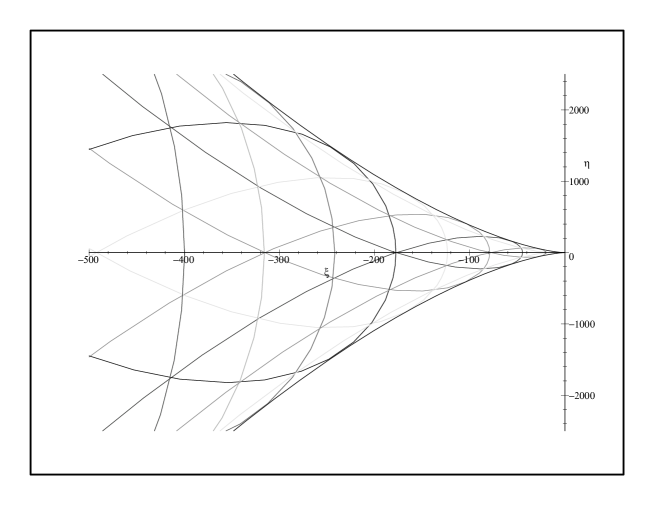
The curves 𝒞 n subscript 𝒞 𝑛 {\cal C}_{n}
𝒞 n : ( 1 + 3 2 ξ n 2 π 2 ) 2 + D 8 n 6 π 6 = 0 : subscript 𝒞 𝑛 superscript 1 3 2 𝜉 superscript 𝑛 2 superscript 𝜋 2 2 𝐷 8 superscript 𝑛 6 superscript 𝜋 6 0 {\cal C}_{n}:\left(1+\frac{3}{2}\frac{\xi}{n^{2}\pi^{2}}\right)^{2}+\frac{D}{8n^{6}\pi^{6}}=0 (4.18)
They were first discovered by numerical computations (Fig. 1).
Figure 1: The zerotrajectories 𝒞 n subscript 𝒞 𝑛 {\cal C}_{n} ( ξ , η ) 𝜉 𝜂 (\xi,\eta)
It is obviously suggesting to attempt a Weierstraß product ansatz
det H ( ξ , η ) = ∏ n = 1 ∞ [ ( 1 + 3 2 ξ n 2 π 2 ) 2 + D 8 n 6 π 6 ] 𝐻 𝜉 𝜂 subscript superscript product 𝑛 1 delimited-[] superscript 1 3 2 𝜉 superscript 𝑛 2 superscript 𝜋 2 2 𝐷 8 superscript 𝑛 6 superscript 𝜋 6 \det H(\xi,\eta)=\prod^{\infty}_{n=1}\left[\left(1+\frac{3}{2}\frac{\xi}{n^{2}\pi^{2}}\right)^{2}+\frac{D}{8n^{6}\pi^{6}}\right] (4.19)
That this is in fact correct can be verified in the following fashion.
Consider the polynomial
x 3 + u x + v = 0 superscript 𝑥 3 𝑢 𝑥 𝑣 0 x^{3}+ux+v=0 (4.20)
with its factorized form
∏ i = 1 3 ( x − α i ) = 0 subscript superscript product 3 𝑖 1 𝑥 subscript 𝛼 𝑖 0 \prod^{3}_{i=1}(x-\alpha_{i})=0 (4.21)
so the elementary symmetric polynomials of { α } i = 1 3 subscript superscript 𝛼 3 𝑖 1 \{\alpha\}^{3}_{i=1}
σ 1 ( α ) = 0 , σ 2 ( α ) = u , σ 3 ( α ) = − v formulae-sequence subscript 𝜎 1 𝛼 0 formulae-sequence subscript 𝜎 2 𝛼 𝑢 subscript 𝜎 3 𝛼 𝑣 \sigma_{1}(\alpha)=0,\,\sigma_{2}(\alpha)=u,\,\sigma_{3}(\alpha)=-v (4.22)
By symmetric evaluation of the product we have
∏ n = − ∞ ( symm . n ≠ 0 ) + ∞ ( 1 − α i n π ) \displaystyle\prod^{+\infty}_{\begin{array}[]{l}{\scriptstyle n=-\infty}\\
{\scriptstyle({\rm symm.}}\\
{\scriptstyle n\not=0)}\end{array}}\left(1-\frac{\alpha_{i}}{n\pi}\right) = \displaystyle= ∏ n = 1 ∞ ( 1 − α i 2 n 2 π 2 ) subscript superscript product 𝑛 1 1 subscript superscript 𝛼 2 𝑖 superscript 𝑛 2 superscript 𝜋 2 \displaystyle\prod^{\infty}_{n=1}\left(1-\frac{\alpha^{2}_{i}}{n^{2}\pi^{2}}\right) (4.26)
= \displaystyle= sin α i α i subscript 𝛼 𝑖 subscript 𝛼 𝑖 \displaystyle\frac{\sin\alpha_{i}}{\alpha_{i}} (4.27)
Correspondingly we get
det H ( ξ , η ) 𝐻 𝜉 𝜂 \displaystyle\det H(\xi,\eta) = \displaystyle= ∏ n = − ∞ ( symm . n ≠ 0 ) + ∞ [ 1 + 3 2 ξ n 2 π 2 + − D 8 1 n 3 π 3 ] \displaystyle\prod^{+\infty}_{\begin{array}[]{l}{\scriptstyle n=-\infty}\\
{\scriptstyle({\rm symm.}}\\
{\scriptstyle n\not=0)}\end{array}}\left[1+\frac{3}{2}\frac{\xi}{n^{2}\pi^{2}}+\sqrt{\frac{-D}{8}}\frac{1}{n^{3}\pi^{3}}\right] (4.31)
= \displaystyle= ∏ i = 1 3 sin α i α i subscript superscript product 3 𝑖 1 subscript 𝛼 𝑖 subscript 𝛼 𝑖 \displaystyle\prod^{3}_{i=1}\frac{\sin\alpha_{i}}{\alpha_{i}} (4.32)
where
u = 3 2 ξ , v = − D 8 formulae-sequence 𝑢 3 2 𝜉 𝑣 𝐷 8 u=\frac{3}{2}\xi,\,v=\sqrt{\frac{-D}{8}} (4.33)
We can expand (4.32 α 1 , α 2 , α 3 subscript 𝛼 1 subscript 𝛼 2 subscript 𝛼 3
\alpha_{1},\alpha_{2},\alpha_{3}
σ 1 ( α ) , σ 2 ( α ) , σ 3 ( α ) . subscript 𝜎 1 𝛼 subscript 𝜎 2 𝛼 subscript 𝜎 3 𝛼
\sigma_{1}(\alpha),\,\sigma_{2}(\alpha),\,\sigma_{3}(\alpha).
Using then (4.22 4.33 4.16
Finally we consider the separatrix
D = 0 implying (say) α 3 = 0 , α 2 = − α 1 formulae-sequence 𝐷 0 formulae-sequence implying (say) subscript 𝛼 3 0 subscript 𝛼 2 subscript 𝛼 1 D=0\quad\mbox{implying (say)}\;\alpha_{3}=0,\,\alpha_{2}=-\alpha_{1} (4.34)
This yields by (4.22 4.33
− σ 2 ( α ) = α 1 2 = − 3 2 ξ subscript 𝜎 2 𝛼 subscript superscript 𝛼 2 1 3 2 𝜉 -\sigma_{2}(\alpha)=\alpha^{2}_{1}=-\frac{3}{2}\xi (4.35)
Then
det H ( ξ , η ) | D = 0 = ( sin α 1 α 1 ) 2 evaluated-at 𝐻 𝜉 𝜂 𝐷 0 superscript subscript 𝛼 1 subscript 𝛼 1 2 \det H(\xi,\eta)|_{D=0}=\left(\frac{\sin\alpha_{1}}{\alpha_{1}}\right)^{2} (4.36)
implying zeros of det H 𝐻 \det H D = 0 𝐷 0 D=0
− 3 2 ξ = ( n π ) 2 , n ∈ 𝖹𝖹 − { 0 } formulae-sequence 3 2 𝜉 superscript 𝑛 𝜋 2 𝑛 𝖹𝖹 0 -\frac{3}{2}\xi=(n\pi)^{2},\;n\in{\mathchoice{\hbox{$\tensans\textstyle Z\kern-5.0ptZ$}}{\hbox{$\tensans\textstyle Z\kern-5.0ptZ$}}{\hbox{$\tensans\scriptstyle Z\kern-2.10002ptZ$}}{\hbox{$\tensans\scriptscriptstyle Z\kern-1.50002ptZ$}}}-\{0\} (4.37)
At this point the zero trajectory 𝒞 n subscript 𝒞 𝑛 {\cal C}_{n}
The representation of the function det H ( ξ , η ) 𝐻 𝜉 𝜂 \det H(\xi,\eta) y 1 , y 2 , y 3 subscript 𝑦 1 subscript 𝑦 2 subscript 𝑦 3
y_{1},y_{2},y_{3} 4.20
α i = 1 2 s 1 2 ( y j − y k ) subscript 𝛼 𝑖 1 2 superscript 𝑠 1 2 subscript 𝑦 𝑗 subscript 𝑦 𝑘 \alpha_{i}=\frac{1}{\sqrt{2}}s^{\frac{1}{2}}(y_{j}-y_{k}) (4.38)
( i , j , k cyclic ) 𝑖 𝑗 𝑘 cyclic (i,j,k\;{\rm cyclic})
Then we find easily
σ 1 ( α ) subscript 𝜎 1 𝛼 \displaystyle\sigma_{1}(\alpha) = \displaystyle= 0 0 \displaystyle 0
σ 2 ( α ) subscript 𝜎 2 𝛼 \displaystyle\sigma_{2}(\alpha) = \displaystyle= 3 2 s σ 2 ( y ) = 3 2 ξ 3 2 𝑠 subscript 𝜎 2 𝑦 3 2 𝜉 \displaystyle\frac{3}{2}s\sigma_{2}(y)=\frac{3}{2}\xi
σ 3 ( α ) subscript 𝜎 3 𝛼 \displaystyle\sigma_{3}(\alpha) = \displaystyle= − s 3 2 V ( y ) 8 = ∓ − D 8 superscript 𝑠 3 2 𝑉 𝑦 8 minus-or-plus 𝐷 8 \displaystyle-s^{\frac{3}{2}}\frac{V(y)}{\sqrt{8}}=\mp\sqrt{\frac{-D}{8}} (4.39)
so that (4.22 4.33 V ( y ) 𝑉 𝑦 V(y) 1.5 y 𝑦 y
y i − y j = 0 , all pairs ( i , j ) i ≠ j formulae-sequence subscript 𝑦 𝑖 subscript 𝑦 𝑗 0 all pairs 𝑖 𝑗 𝑖 𝑗 y_{i}-y_{j}=0,\;\mbox{all pairs}\;(i,j)\;i\not=j (4.40)
cutting the plane into six sectors. They correspond to the six elements of the symmetric
group S 3 subscript 𝑆 3 S_{3} 1.15 1.18 4.32 4.38 𝒞 n subscript 𝒞 𝑛 {\cal C}_{n}
1 2 s 1 2 ( y i − y j ) = n π , n ∈ I N , all pairs ( i , j ) i ≠ j formulae-sequence 1 2 superscript 𝑠 1 2 subscript 𝑦 𝑖 subscript 𝑦 𝑗 𝑛 𝜋 formulae-sequence 𝑛 I N all pairs 𝑖 𝑗 𝑖 𝑗 \frac{1}{\sqrt{2}}s^{\frac{1}{2}}(y_{i}-y_{j})=n\pi,\;n\in{\rm I\!N},\;\mbox{all pairs}\;(i,j)\;i\not=j (4.41)
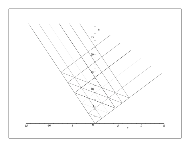
Three of these lines intersect the same sector and these lines intersect each other on the
boundary of the sector, i.e. on the separatrix. In Fig. 2 we present the resulting image
for the identity element of S 3 subscript 𝑆 3 S_{3} ( y 2 , y 3 ) subscript 𝑦 2 subscript 𝑦 3 (y_{2},y_{3})
Figure 2: The sectorE 1 subscript 𝐸 1 E_{1} ( y 2 , y 3 ) subscript 𝑦 2 subscript 𝑦 3 (y_{2},y_{3}) 1 ≤ n ≤ 5 1 𝑛 5 1\leq n\leq 5
5 The spectrum
On the linear space (1.31
V n = ⨁ m = 0 n U m subscript 𝑉 𝑛 subscript superscript direct-sum 𝑛 𝑚 0 subscript 𝑈 𝑚 V_{n}=\bigoplus\limits^{n}_{m=0}U_{m} (5.1)
we consider the quadratic operator
− ( ∂ ∂ ξ , ∂ ∂ η ) Γ ( ξ , η ) ( ∂ ∂ ξ ∂ ∂ η ) 𝜉 𝜂 Γ 𝜉 𝜂 𝜉 𝜂 -\left(\frac{\partial}{\partial\xi},\frac{\partial}{\partial\eta}\right)\Gamma(\xi,\eta)\left(\begin{array}[]{c}\frac{\partial}{\partial\xi}\\
\frac{\partial}{\partial\eta}\end{array}\right) (5.2)
(differentiation of Γ Γ \Gamma Γ Γ \Gamma 4.5 𝒜 + ℬ 𝒜 ℬ {\cal A}+{\cal B} m 𝑚 m
𝒜 U m ⊂ U m , ℬ U m + 1 ⊂ U m formulae-sequence 𝒜 subscript 𝑈 𝑚 subscript 𝑈 𝑚 ℬ subscript 𝑈 𝑚 1 subscript 𝑈 𝑚 {\cal A}U_{m}\subset U_{m},\;{\cal B}U_{m+1}\subset U_{m} (5.3)
Now we span U m subscript 𝑈 𝑚 U_{m} m 𝑚 m
∑ r = 0 m a r ( m ) ξ r η m − r subscript superscript 𝑚 𝑟 0 subscript superscript 𝑎 𝑚 𝑟 superscript 𝜉 𝑟 superscript 𝜂 𝑚 𝑟 \sum^{m}_{r=0}a^{(m)}_{r}\xi^{r}\eta^{m-r} (5.4)
then the map 𝒜 𝒜 {\cal A}
a r ( m ) → 𝒜 a r ′ ( m ) subscript superscript 𝑎 𝑚 𝑟 → 𝒜 subscript superscript 𝑎 ′ 𝑚
𝑟 \displaystyle a^{(m)}_{r}\begin{array}[]{c}\to\\
{\cal A}\end{array}a^{\prime(m)}_{r} = \displaystyle= [ m 2 + 7 3 m + 2 3 r ( m − r ) ] a r ( m ) delimited-[] superscript 𝑚 2 7 3 𝑚 2 3 𝑟 𝑚 𝑟 subscript superscript 𝑎 𝑚 𝑟 \displaystyle[m^{2}+\frac{7}{3}m+\frac{2}{3}r(m-r)]a^{(m)}_{r} (5.8)
− 2 3 ( m − r + 2 ) ( m − r + 1 ) a r − 2 ( m ) 2 3 𝑚 𝑟 2 𝑚 𝑟 1 subscript superscript 𝑎 𝑚 𝑟 2 \displaystyle-\frac{2}{3}(m-r+2)(m-r+1)a^{(m)}_{r-2}
− 1 6 ( r + 2 ) ( r + 1 ) a r + 2 ( m ) 1 6 𝑟 2 𝑟 1 subscript superscript 𝑎 𝑚 𝑟 2 \displaystyle-\frac{1}{6}(r+2)(r+1)a^{(m)}_{r+2}
a r ( m ) → ℬ a r ′ ( m − 1 ) = ( r + 1 ) ( 6 m − 4 r − 1 ) a r + 1 ( m ) a^{(m)}_{r}\begin{array}[]{c}\to\\
{\cal B}\end{array}a_{r}^{\prime(m-1})=(r+1)(6m-4r-1)a_{r+1}^{(m)} (5.9)
From (5.8 5.9 U m subscript 𝑈 𝑚 U_{m} r 𝑟 r ξ 𝜉 \xi
U m = U m ( + ) ⊕ U m ( − ) subscript 𝑈 𝑚 direct-sum superscript subscript 𝑈 𝑚 superscript subscript 𝑈 𝑚 U_{m}=U_{m}^{(+)}\oplus U_{m}^{(-)} (5.10)
U m ( + ) = span { ξ 2 r η m − 2 r } r = 0 [ m 2 ] superscript subscript 𝑈 𝑚 span subscript superscript superscript 𝜉 2 𝑟 superscript 𝜂 𝑚 2 𝑟 delimited-[] 𝑚 2 𝑟 0 U_{m}^{(+)}={\rm span}\{\xi^{2r}\eta^{m-2r}\}^{\left[\frac{m}{2}\right]}_{r=0} (5.11)
U m ( − ) = span { ξ 2 r + 1 η m − 2 r − 1 } r = 0 [ m − 1 2 ] superscript subscript 𝑈 𝑚 span subscript superscript superscript 𝜉 2 𝑟 1 superscript 𝜂 𝑚 2 𝑟 1 delimited-[] 𝑚 1 2 𝑟 0 U_{m}^{(-)}={\rm span}\{\xi^{2r+1}\eta^{m-2r-1}\}^{\left[\frac{m-1}{2}\right]}_{r=0} (5.12)
so that
𝒜 U m ( ± ) ⊂ U m ( ± ) 𝒜 superscript subscript 𝑈 𝑚 plus-or-minus superscript subscript 𝑈 𝑚 plus-or-minus \displaystyle{\cal A}U_{m}^{(\pm)}\subset U_{m}^{(\pm)}
ℬ U m ( ± ) ⊂ U m − 1 ( ∓ ) ℬ superscript subscript 𝑈 𝑚 plus-or-minus superscript subscript 𝑈 𝑚 1 minus-or-plus \displaystyle{\cal B}U_{m}^{(\pm)}\subset U_{m-1}^{(\mp)} (5.13)
Correspondingly the set of eigenvalues Λ ( m ) superscript Λ 𝑚 \Lambda^{(m)} 𝒜 𝒜 {\cal A} U m subscript 𝑈 𝑚 U_{m}
Λ m = Λ m ( + ) ∪ Λ m ( − ) subscript Λ 𝑚 superscript subscript Λ 𝑚 superscript subscript Λ 𝑚 \Lambda_{m}=\Lambda_{m}^{(+)}\cup\Lambda_{m}^{(-)} (5.14)
The eigenvalues on each subspace U m ( ± ) superscript subscript 𝑈 𝑚 plus-or-minus U_{m}^{(\pm)} m 𝑚 m
For the even part we find
Λ m ( + ) = { 1 3 [ 4 m 2 − ( 4 r − 10 ) m + 4 ( r − 1 ) 2 ] ; \displaystyle\Lambda_{m}^{(+)}=\{\frac{1}{3}[4m^{2}-(4r-10)m+4(r-1)^{2}];
r ∈ { 1 , 2 , … , [ m 2 ] + 1 } } \displaystyle r\in\{1,2,\ldots,[\frac{m}{2}]+1\}\} (5.15)
For increasing r 𝑟 r λ r ( m ) superscript subscript 𝜆 𝑟 𝑚 \lambda_{r}^{(m)}
Λ m ( − ) superscript subscript Λ 𝑚 \displaystyle\Lambda_{m}^{(-)} = \displaystyle= Λ m ( + ) , m odd superscript subscript Λ 𝑚 m odd
\displaystyle\Lambda_{m}^{(+)},\quad\mbox{$m$ odd}
Λ m ( − ) superscript subscript Λ 𝑚 \displaystyle\Lambda_{m}^{(-)} = \displaystyle= Λ m ( + ) − { m 2 + 2 m } , m even superscript subscript Λ 𝑚 superscript 𝑚 2 2 𝑚 m even
\displaystyle\Lambda_{m}^{(+)}-\{m^{2}+2m\},\quad\mbox{$m$ even} (5.16)
where m 2 + 2 m superscript 𝑚 2 2 𝑚 m^{2}+2m Λ m ( + ) superscript subscript Λ 𝑚 \Lambda_{m}^{(+)}
On V n subscript 𝑉 𝑛 V_{n} 5.1 𝒜 + ℬ 𝒜 ℬ {\cal A}+{\cal B}
( 𝒜 n , 0 ℬ n , 𝒜 ( n − 1 ) 0 0 ℬ ( n − 1 ) 𝒜 ( n − 2 ) 0 0 ℬ ( n − 2 ) 𝒜 ( n − 3 ) 0 ℬ 2 𝒜 1 0 0 ℬ 1 𝒜 0 ) subscript 𝒜 𝑛 0 missing-subexpression missing-subexpression missing-subexpression missing-subexpression missing-subexpression missing-subexpression subscript ℬ 𝑛 subscript 𝒜 𝑛 1 0 missing-subexpression missing-subexpression missing-subexpression missing-subexpression missing-subexpression 0 subscript ℬ 𝑛 1 subscript 𝒜 𝑛 2 0 missing-subexpression missing-subexpression missing-subexpression missing-subexpression missing-subexpression 0 subscript ℬ 𝑛 2 subscript 𝒜 𝑛 3 missing-subexpression missing-subexpression missing-subexpression missing-subexpression missing-subexpression missing-subexpression missing-subexpression missing-subexpression missing-subexpression 0 missing-subexpression missing-subexpression missing-subexpression missing-subexpression missing-subexpression missing-subexpression missing-subexpression subscript ℬ 2 subscript 𝒜 1 0 missing-subexpression missing-subexpression missing-subexpression missing-subexpression missing-subexpression 0 subscript ℬ 1 subscript 𝒜 0 \left(\begin{array}[]{cccccccc}{\cal A}_{n},&0\\
{\cal B}_{n},&{\cal A}_{(n-1)}&0&&\\
0&{\cal B}_{(n-1)}&{\cal A}_{(n-2)}&0\\
&0&{\cal B}_{(n-2)}&{\cal A}_{(n-3)}&\\
&&&&&0\\
&&&&&{\cal B}_{2}&{\cal A}_{1}&0\\
&&&&&0&{\cal B}_{1}&{\cal A}_{0}\end{array}\right) (5.17)
where 𝒜 m ( ℬ m ) subscript 𝒜 𝑚 subscript ℬ 𝑚 {\cal A}_{m}({\cal B}_{m}) 𝒜 ( ℬ ) 𝒜 ℬ {\cal A}({\cal B}) U m subscript 𝑈 𝑚 U_{m} V n subscript 𝑉 𝑛 V_{n} V m ( m < n ) subscript 𝑉 𝑚 𝑚 𝑛 V_{m}(m<n)
Λ m ∩ Λ m ′ = ϕ for m ≠ m ′ subscript Λ 𝑚 subscript Λ superscript 𝑚 ′ italic-ϕ for 𝑚 superscript 𝑚 ′ \Lambda_{m}\cap\Lambda_{m^{\prime}}=\phi\;\,{\rm for}\;\,m\not=m^{\prime} (5.18)
then
𝒜 n e n = λ r ( n ) e n , e n ∈ U n formulae-sequence subscript 𝒜 𝑛 subscript 𝑒 𝑛 superscript subscript 𝜆 𝑟 𝑛 subscript 𝑒 𝑛 subscript 𝑒 𝑛 subscript 𝑈 𝑛 {\cal A}_{n}e_{n}=\lambda_{r}^{(n)}e_{n},\quad e_{n}\in U_{n} (5.19)
implies for the component e m subscript 𝑒 𝑚 e_{m} U m , m < n subscript 𝑈 𝑚 𝑚
𝑛 U_{m},\,m<n
e m = − ( 𝒜 m − λ r ( m ) E ) − 1 ℬ ( m + 1 ) e ( m + 1 ) subscript 𝑒 𝑚 superscript subscript 𝒜 𝑚 superscript subscript 𝜆 𝑟 𝑚 𝐸 1 subscript ℬ 𝑚 1 subscript 𝑒 𝑚 1 e_{m}=-({\cal A}_{m}-\lambda_{r}^{(m)}E)^{-1}{\cal B}_{(m+1)}e_{(m+1)} (5.20)
However, (5.18
λ 1 ( 14 ) = λ 8 ( 16 ) = 868 3 λ 1 ( 27 ) = λ 15 ( 31 ) = 1026 λ 2 ( 18 ) = λ 9 ( 20 ) = 1336 3 λ 6 ( 30 ) = λ 15 ( 32 ) = 3280 3 λ 3 ( 22 ) = λ 10 ( 24 ) = 636 λ 5 ( 30 ) = λ 12 ( 32 ) = 3364 3 λ 1 ( 22 ) = λ 6 ( 24 ) = 2068 3 λ 2 ( 30 ) = λ 7 ( 32 ) = 3664 3 λ 4 ( 26 ) = λ 11 ( 28 ) = 2584 3 λ 2 ( 31 ) = λ 16 ( 35 ) = 3910 3 superscript subscript 𝜆 1 14 superscript subscript 𝜆 8 16 868 3 superscript subscript 𝜆 1 27 superscript subscript 𝜆 15 31 1026 superscript subscript 𝜆 2 18 superscript subscript 𝜆 9 20 1336 3 superscript subscript 𝜆 6 30 superscript subscript 𝜆 15 32 3280 3 superscript subscript 𝜆 3 22 superscript subscript 𝜆 10 24 636 superscript subscript 𝜆 5 30 superscript subscript 𝜆 12 32 3364 3 superscript subscript 𝜆 1 22 superscript subscript 𝜆 6 24 2068 3 superscript subscript 𝜆 2 30 superscript subscript 𝜆 7 32 3664 3 superscript subscript 𝜆 4 26 superscript subscript 𝜆 11 28 2584 3 superscript subscript 𝜆 2 31 superscript subscript 𝜆 16 35 3910 3 \begin{array}[]{rclcl@{\qquad}rclcl}\lambda_{1}^{(14)}&=&\lambda_{8}^{(16)}&=&\frac{868}{3}&\quad\lambda_{1}^{(27)}&=&\lambda_{15}^{(31)}&=&1026\\
\lambda_{2}^{(18)}&=&\lambda_{9}^{(20)}&=&\frac{1336}{3}&\lambda_{6}^{(30)}&=&\lambda_{15}^{(32)}&=&\frac{3280}{3}\\
\lambda_{3}^{(22)}&=&\lambda_{10}^{(24)}&=&636&\lambda_{5}^{(30)}&=&\lambda_{12}^{(32)}&=&\frac{3364}{3}\\
\lambda_{1}^{(22)}&=&\lambda_{6}^{(24)}&=&\frac{2068}{3}&\lambda_{2}^{(30)}&=&\lambda_{7}^{(32)}&=&\frac{3664}{3}\\
\lambda_{4}^{(26)}&=&\lambda_{11}^{(28)}&=&\frac{2584}{3}&\lambda_{2}^{(31)}&=&\lambda_{16}^{(35)}&=&\frac{3910}{3}\end{array} (5.21)
Two eigenvalues can only coincide if m 1 − m 2 subscript 𝑚 1 subscript 𝑚 2 m_{1}-m_{2} m 1 , m 2 subscript 𝑚 1 subscript 𝑚 2
m_{1},m_{2} m 1 < m 2 , r 1 < r 2 formulae-sequence subscript 𝑚 1 subscript 𝑚 2 subscript 𝑟 1 subscript 𝑟 2 m_{1}<m_{2},r_{1}<r_{2}
( 𝒜 m 1 − λ r 2 ( m 2 ) E ) − 1 superscript subscript 𝒜 subscript 𝑚 1 superscript subscript 𝜆 subscript 𝑟 2 subscript 𝑚 2 𝐸 1 ({\cal A}_{m_{1}}-\lambda_{r_{2}}^{(m_{2})}E)^{-1}
does not exist. But in addition
ℬ m 1 + 1 e m 1 + 1 ≠ 0 subscript ℬ subscript 𝑚 1 1 subscript 𝑒 subscript 𝑚 1 1 0 {\cal B}_{m_{1}+1}e_{m_{1}+1}\not=0 (5.22)
since ℬ m subscript ℬ 𝑚 {\cal B}_{m} 5.9
Thus the eigenvectors in V m 2 subscript 𝑉 subscript 𝑚 2 V_{m_{2}} λ r 2 ( m 2 ) superscript subscript 𝜆 subscript 𝑟 2 subscript 𝑚 2 \lambda_{r_{2}}^{(m_{2})} ξ 𝜉 \xi η 𝜂 \eta 5.2
This incompleteness can be cured by adding a linear term in the Lie algebra to (5.2
+ γ ( ξ ∂ ∂ ξ + η ∂ ∂ η ) , γ ∉ Q 𝛾 𝜉 𝜉 𝜂 𝜂 𝛾
Q +\gamma\left(\xi\frac{\partial}{\partial\xi}+\eta\frac{\partial}{\partial\eta}\right),\;\gamma\notin{\mathchoice{\hbox{\raise 1.02495pt\hbox to0.0pt{\kern 3.11107pt\vrule height=5.46666pt\hss}\hbox{$\displaystyle\rm Q$}}}{\hbox{\raise 1.02495pt\hbox to0.0pt{\kern 3.11107pt\vrule height=5.46666pt\hss}\hbox{$\textstyle\rm Q$}}}{\hbox{\raise 0.71747pt\hbox to0.0pt{\kern 2.17775pt\vrule height=3.34831pt\hss}\hbox{$\scriptstyle\rm Q$}}}{\hbox{\raise 0.51247pt\hbox to0.0pt{\kern 1.55553pt\vrule height=2.39165pt\hss}\hbox{$\scriptscriptstyle\rm Q$}}}} (5.23)
In fact we shall see in the subsequent section that such term is essential for self-adjointness of the
Schrödinger operator.
6 The Schrödinger operator
We start from (3.19
Q = − ∑ a , b ∂ ∂ τ a g a b − 1 ∂ ∂ τ b + γ ∑ a r a ∂ ∂ τ a 𝑄 subscript 𝑎 𝑏
subscript 𝜏 𝑎 subscript superscript 𝑔 1 𝑎 𝑏 subscript 𝜏 𝑏 𝛾 subscript 𝑎 subscript 𝑟 𝑎 subscript 𝜏 𝑎 Q=-\sum_{a,b}\frac{\partial}{\partial\tau_{a}}g^{-1}_{ab}\frac{\partial}{\partial\tau_{b}}+\gamma\sum_{a}r_{a}\frac{\partial}{\partial\tau_{a}} (6.1)
where γ ∈ I R 𝛾 I R \gamma\in{\rm I\!R} r a ( τ ) subscript 𝑟 𝑎 𝜏 r_{a}(\tau) { τ a } subscript 𝜏 𝑎 \{\tau_{a}\} Q 𝑄 Q φ 𝜑 \varphi ϵ italic-ϵ \epsilon
Q φ = ϵ φ 𝑄 𝜑 italic-ϵ 𝜑 Q\varphi=\epsilon\varphi (6.2)
By an appropriate choice of a gauge function χ 𝜒 \chi
φ = e χ ψ 𝜑 superscript 𝑒 𝜒 𝜓 \varphi=e^{\chi}\psi (6.3)
we want to transform Q 𝑄 Q τ 𝜏 \tau
− Δ ψ + W ψ = ϵ ψ Δ 𝜓 𝑊 𝜓 italic-ϵ 𝜓 -\Delta\psi+W\psi=\epsilon\psi (6.4)
Here Δ Δ \Delta
Δ = 1 g ∑ a , b ∂ ∂ τ a g g a b − 1 ∂ ∂ τ b Δ 1 𝑔 subscript 𝑎 𝑏
subscript 𝜏 𝑎 𝑔 subscript superscript 𝑔 1 𝑎 𝑏 subscript 𝜏 𝑏 \Delta=\frac{1}{\sqrt{g}}\sum_{a,b}\frac{\partial}{\partial\tau_{a}}\sqrt{g}g^{-1}_{ab}\frac{\partial}{\partial\tau_{b}} (6.5)
and W 𝑊 W χ 𝜒 \chi γ 𝛾 \gamma g 𝑔 g
g = ( det { g a b − 1 } ) − 1 𝑔 superscript subscript superscript 𝑔 1 𝑎 𝑏 1 g=(\det\{g^{-1}_{ab}\})^{-1} (6.6)
and comes out from (3.19
g ( s ; τ ) − 1 = − 1 3 { ( 4 τ 2 3 + 27 τ 3 2 ) + 2 s τ 2 ( τ 2 3 + 9 τ 3 2 ) \displaystyle g(s;\tau)^{-1}=-\frac{1}{3}\big{\{}(4\tau^{3}_{2}+27\tau^{2}_{3})+2s\tau_{2}(\tau^{3}_{2}+9\tau^{2}_{3})
+ 2 s 2 τ 2 2 τ 3 2 + 1 2 s 3 τ 3 4 } \displaystyle+2s^{2}\tau^{2}_{2}\tau^{2}_{3}+\frac{1}{2}s^{3}\tau^{4}_{3}\big{\}} (6.7)
This function can be expressed by { τ a ′ } subscript superscript 𝜏 ′ 𝑎 \{\tau^{\prime}_{a}\} 4.1
g ( s ; τ ( τ ′ ) ) − 1 = − 1 3 ( 4 τ 2 ′ 3 + 27 τ 3 ′ 2 ) ⋅ ( det Ω ( τ ′ ) ) 2 𝑔 superscript 𝑠 𝜏 superscript 𝜏 ′
1 ⋅ 1 3 4 subscript superscript 𝜏 ′ 3
2 27 subscript superscript 𝜏 ′ 2
3 superscript Ω superscript 𝜏 ′ 2 g(s;\tau(\tau^{\prime}))^{-1}=-\frac{1}{3}(4\tau^{\prime 3}_{2}+27\tau^{\prime 2}_{3})\cdot(\det\Omega(\tau^{\prime}))^{2} (6.8)
After multiplication with appropriate powers of s 𝑠 s 4.8
Γ ( ξ , η ) = − 1 3 D ( ξ ′ , η ′ ) ( det H ( ξ ′ , η ′ ) ) 2 Γ 𝜉 𝜂 1 3 𝐷 superscript 𝜉 ′ superscript 𝜂 ′ superscript 𝐻 superscript 𝜉 ′ superscript 𝜂 ′ 2 \Gamma(\xi,\eta)=-\frac{1}{3}D(\xi^{\prime},\eta^{\prime})(\det H(\xi^{\prime},\eta^{\prime}))^{2} (6.9)
where Γ Γ \Gamma 4.5
In order to fix χ 𝜒 \chi
e − χ Q e χ superscript 𝑒 𝜒 𝑄 superscript 𝑒 𝜒 \displaystyle e^{-\chi}Qe^{\chi} = \displaystyle= − ∑ a , b ( ∂ ∂ τ a + ∂ χ ∂ τ a ) g a b − 1 ( ∂ ∂ τ b + ∂ χ ∂ τ b ) subscript 𝑎 𝑏
subscript 𝜏 𝑎 𝜒 subscript 𝜏 𝑎 subscript superscript 𝑔 1 𝑎 𝑏 subscript 𝜏 𝑏 𝜒 subscript 𝜏 𝑏 \displaystyle-\sum_{a,b}\left(\frac{\partial}{\partial\tau_{a}}+\frac{\partial\chi}{\partial\tau_{a}}\right)g^{-1}_{ab}\left(\frac{\partial}{\partial\tau_{b}}+\frac{\partial\chi}{\partial\tau_{b}}\right) (6.10)
+ γ ∑ a r a ( ∂ ∂ τ a + ∂ χ ∂ τ a ) 𝛾 subscript 𝑎 subscript 𝑟 𝑎 subscript 𝜏 𝑎 𝜒 subscript 𝜏 𝑎 \displaystyle+\gamma\sum_{a}r_{a}\left(\frac{\partial}{\partial\tau_{a}}+\frac{\partial\chi}{\partial\tau_{a}}\right)
We match the first order differential operator parts in (6.4 6.5 6.10
− 2 ∑ a ∂ χ ∂ τ a g a b − 1 + γ r b = − ∑ a ∂ ∂ τ a ( ln g ) g a b − 1 2 subscript 𝑎 𝜒 subscript 𝜏 𝑎 subscript superscript 𝑔 1 𝑎 𝑏 𝛾 subscript 𝑟 𝑏 subscript 𝑎 subscript 𝜏 𝑎 𝑔 subscript superscript 𝑔 1 𝑎 𝑏 -2\sum_{a}\frac{\partial\chi}{\partial\tau_{a}}g^{-1}_{ab}+\gamma r_{b}=-\sum_{a}\frac{\partial}{\partial\tau_{a}}(\ln\sqrt{g})g^{-1}_{ab} (6.11)
The integrability condition for this differential equation is
∂ ∂ τ a ∑ c r c g c b = ∂ ∂ τ b ∑ c r c g c a subscript 𝜏 𝑎 subscript 𝑐 subscript 𝑟 𝑐 subscript 𝑔 𝑐 𝑏 subscript 𝜏 𝑏 subscript 𝑐 subscript 𝑟 𝑐 subscript 𝑔 𝑐 𝑎 \frac{\partial}{\partial\tau_{a}}\sum_{c}r_{c}g_{cb}=\frac{\partial}{\partial\tau_{b}}\sum_{c}r_{c}g_{ca} (6.12)
If (6.12 ρ 𝜌 \rho
r a = ∑ b g a b − 1 ∂ ∂ τ b ρ subscript 𝑟 𝑎 subscript 𝑏 subscript superscript 𝑔 1 𝑎 𝑏 subscript 𝜏 𝑏 𝜌 r_{a}=\sum_{b}g^{-1}_{ab}\frac{\partial}{\partial\tau_{b}}\rho (6.13)
In fact, we can show easily that
ρ = ln g 𝜌 𝑔 \rho=\ln\sqrt{g} (6.14)
and
r 2 subscript 𝑟 2 \displaystyle r_{2} = \displaystyle= 3 + 2 s τ 2 3 2 𝑠 subscript 𝜏 2 \displaystyle 3+2s\tau_{2}
r 3 subscript 𝑟 3 \displaystyle r_{3} = \displaystyle= 2 s τ 3 2 𝑠 subscript 𝜏 3 \displaystyle 2s\tau_{3} (6.15)
fulfill (6.12 6.13 6.11
χ = 1 2 ( 1 + γ ) ln g 𝜒 1 2 1 𝛾 𝑔 \chi=\frac{1}{2}(1+\gamma)\ln\sqrt{g} (6.16)
and the potential comes out as
W ( τ ) 𝑊 𝜏 \displaystyle W(\tau) = \displaystyle= − ∑ a , b { ∂ ∂ τ a ( g a b − 1 ∂ χ ∂ τ b ) + g a b − 1 ∂ χ ∂ τ a ∂ χ ∂ τ b } subscript 𝑎 𝑏
subscript 𝜏 𝑎 subscript superscript 𝑔 1 𝑎 𝑏 𝜒 subscript 𝜏 𝑏 subscript superscript 𝑔 1 𝑎 𝑏 𝜒 subscript 𝜏 𝑎 𝜒 subscript 𝜏 𝑏 \displaystyle-\sum_{a,b}\left\{\frac{\partial}{\partial\tau_{a}}\left(g^{-1}_{ab}\frac{\partial\chi}{\partial\tau_{b}}\right)+g^{-1}_{ab}\frac{\partial\chi}{\partial\tau_{a}}\frac{\partial\chi}{\partial\tau_{b}}\right\} (6.17)
+ γ ∑ a r a ∂ χ ∂ τ a 𝛾 subscript 𝑎 subscript 𝑟 𝑎 𝜒 subscript 𝜏 𝑎 \displaystyle+\gamma\sum_{a}r_{a}\frac{\partial\chi}{\partial\tau_{a}}
Due to (6.13 6.15
W ( τ ) = 1 4 ( γ 2 − 1 ) ∑ a , b g a b − 1 ∂ ln g ∂ τ a ∂ ln g ∂ τ b + const 𝑊 𝜏 1 4 superscript 𝛾 2 1 subscript 𝑎 𝑏
subscript superscript 𝑔 1 𝑎 𝑏 𝑔 subscript 𝜏 𝑎 𝑔 subscript 𝜏 𝑏 const W(\tau)=\frac{1}{4}(\gamma^{2}-1)\sum_{a,b}g^{-1}_{ab}\frac{\partial\ln\sqrt{g}}{\partial\tau_{a}}\frac{\partial\ln\sqrt{g}}{\partial\tau_{b}}+\,{\rm const} (6.18)
The wave functions
ψ = e − χ φ = g − 1 4 ( 1 + γ ) φ 𝜓 superscript 𝑒 𝜒 𝜑 superscript 𝑔 1 4 1 𝛾 𝜑 \psi=e^{-\chi}\varphi=g^{-\frac{1}{4}(1+\gamma)}\varphi (6.19)
have a zero of order 1 2 ( 1 + γ ) 1 2 1 𝛾 \frac{1}{2}(1+\gamma) 𝒞 n subscript 𝒞 𝑛 {\cal C}_{n}
g − 1 2 = const . | ∏ i < j sin s 2 ( y i − y j ) | formulae-sequence superscript 𝑔 1 2 const subscript product 𝑖 𝑗 𝑠 2 subscript 𝑦 𝑖 subscript 𝑦 𝑗 g^{-\frac{1}{2}}={\rm const.}\,|\prod_{i<j}\sin\sqrt{\frac{s}{2}}(y_{i}-y_{j})| (6.20)
which follows from (4.17 4.32 4.38 6.9 γ 𝛾 \gamma s = 1 𝑠 1 s=1 6.15 r 2 subscript 𝑟 2 r_{2} r 3 subscript 𝑟 3 r_{3} 5.23
(1)
for γ = 0 𝛾 0 \gamma=0
(2)
for γ > 0 𝛾 0 \gamma>0 γ ∉ Q 𝛾 Q \gamma\notin{\mathchoice{\hbox{\raise 1.02495pt\hbox to0.0pt{\kern 3.11107pt\vrule height=5.46666pt\hss}\hbox{$\displaystyle\rm Q$}}}{\hbox{\raise 1.02495pt\hbox to0.0pt{\kern 3.11107pt\vrule height=5.46666pt\hss}\hbox{$\textstyle\rm Q$}}}{\hbox{\raise 0.71747pt\hbox to0.0pt{\kern 2.17775pt\vrule height=3.34831pt\hss}\hbox{$\scriptstyle\rm Q$}}}{\hbox{\raise 0.51247pt\hbox to0.0pt{\kern 1.55553pt\vrule height=2.39165pt\hss}\hbox{$\scriptscriptstyle\rm Q$}}}} 1.3
γ = 2 ν − 1 , ν ∈ 𝖹𝖹 formulae-sequence 𝛾 2 𝜈 1 𝜈 𝖹𝖹 \gamma=2\nu-1,\quad\nu\in{\mathchoice{\hbox{$\tensans\textstyle Z\kern-5.0ptZ$}}{\hbox{$\tensans\textstyle Z\kern-5.0ptZ$}}{\hbox{$\tensans\scriptstyle Z\kern-2.10002ptZ$}}{\hbox{$\tensans\scriptscriptstyle Z\kern-1.50002ptZ$}}} (6.21)
insertion of (6.20 6.18 [7 ] , which is known
to be exactly soluble.
The wavefunctions ψ 𝜓 \psi E g subscript 𝐸 𝑔 E_{g} y 𝑦 y
𝒞 n 1 , 𝒞 n 2 , 𝒞 n 3 : : subscript 𝒞 subscript 𝑛 1 subscript 𝒞 subscript 𝑛 2 subscript 𝒞 subscript 𝑛 3
absent \displaystyle{\cal C}_{n_{1}},\;{\cal C}_{n_{2}},\;{\cal C}_{n_{3}}:
n 1 ≤ n 2 ≤ n 3 , n 3 = n 1 + n 2 ± 1 formulae-sequence subscript 𝑛 1 subscript 𝑛 2 subscript 𝑛 3 subscript 𝑛 3 plus-or-minus subscript 𝑛 1 subscript 𝑛 2 1 \displaystyle n_{1}\leq n_{2}\leq n_{3},\;n_{3}=n_{1}+n_{2}\pm 1 (6.22)
7 The N = 4 𝑁 4 N=4
The Calogero model for N = 3 𝑁 3 N=3 1.1 N = 4 𝑁 4 N=4 s , w 3 , w 4 𝑠 subscript 𝑤 3 subscript 𝑤 4
s,w_{3},w_{4} 3.16 3.17
g 22 − 1 subscript superscript 𝑔 1 22 \displaystyle g^{-1}_{22} = \displaystyle= − 2 τ 2 − ( τ 2 2 + a 1 w 4 τ 4 ) s 2 subscript 𝜏 2 subscript superscript 𝜏 2 2 subscript 𝑎 1 subscript 𝑤 4 subscript 𝜏 4 𝑠 \displaystyle-2\tau_{2}-(\tau^{2}_{2}+a_{1}w_{4}\tau_{4})s (7.1)
− ( a 2 w 3 2 τ 3 2 − a 3 w 4 τ 2 τ 4 ) s 2 subscript 𝑎 2 subscript superscript 𝑤 2 3 subscript superscript 𝜏 2 3 subscript 𝑎 3 subscript 𝑤 4 subscript 𝜏 2 subscript 𝜏 4 superscript 𝑠 2 \displaystyle-(a_{2}w^{2}_{3}\tau^{2}_{3}-a_{3}w_{4}\tau_{2}\tau_{4})s^{2}
− a 4 w 4 2 τ 4 2 s 3 subscript 𝑎 4 subscript superscript 𝑤 2 4 subscript superscript 𝜏 2 4 superscript 𝑠 3 \displaystyle-a_{4}w^{2}_{4}\tau^{2}_{4}s^{3}
g 23 − 1 = − 3 τ 3 − a 5 τ 2 τ 3 s − a 6 w 4 τ 3 τ 4 s 2 subscript superscript 𝑔 1 23 3 subscript 𝜏 3 subscript 𝑎 5 subscript 𝜏 2 subscript 𝜏 3 𝑠 subscript 𝑎 6 subscript 𝑤 4 subscript 𝜏 3 subscript 𝜏 4 superscript 𝑠 2 g^{-1}_{23}=-3\tau_{3}-a_{5}\tau_{2}\tau_{3}s-a_{6}w_{4}\tau_{3}\tau_{4}s^{2} (7.2)
g 24 − 1 subscript superscript 𝑔 1 24 \displaystyle g^{-1}_{24} = \displaystyle= − 4 τ 4 − ( a 7 τ 2 τ 4 + a 8 w 4 − 1 w 3 2 τ 3 2 ) s 4 subscript 𝜏 4 subscript 𝑎 7 subscript 𝜏 2 subscript 𝜏 4 subscript 𝑎 8 superscript subscript 𝑤 4 1 subscript superscript 𝑤 2 3 superscript subscript 𝜏 3 2 𝑠 \displaystyle-4\tau_{4}-(a_{7}\tau_{2}\tau_{4}+a_{8}w_{4}^{-1}w^{2}_{3}\tau_{3}^{2})s (7.3)
− a 9 w 4 τ 4 2 s 2 subscript 𝑎 9 subscript 𝑤 4 subscript superscript 𝜏 2 4 superscript 𝑠 2 \displaystyle-a_{9}w_{4}\tau^{2}_{4}s^{2}
g 33 − 1 subscript superscript 𝑔 1 33 \displaystyle g^{-1}_{33} = \displaystyle= − 4 w 4 w 3 − 2 τ 4 + w 3 − 2 τ 2 2 4 subscript 𝑤 4 subscript superscript 𝑤 2 3 subscript 𝜏 4 subscript superscript 𝑤 2 3 subscript superscript 𝜏 2 2 \displaystyle-4w_{4}w^{-2}_{3}\tau_{4}+w^{-2}_{3}\tau^{2}_{2} (7.4)
− ( a 10 w 4 w 3 − 2 τ 2 τ 4 + a 11 τ 3 2 ) s subscript 𝑎 10 subscript 𝑤 4 subscript superscript 𝑤 2 3 subscript 𝜏 2 subscript 𝜏 4 subscript 𝑎 11 subscript superscript 𝜏 2 3 𝑠 \displaystyle-(a_{10}w_{4}w^{-2}_{3}\tau_{2}\tau_{4}+a_{11}\tau^{2}_{3})s
− a 12 w 4 2 w 3 − 2 τ 4 2 s 2 subscript 𝑎 12 subscript superscript 𝑤 2 4 subscript superscript 𝑤 2 3 subscript superscript 𝜏 2 4 superscript 𝑠 2 \displaystyle-a_{12}w^{2}_{4}w^{-2}_{3}\tau^{2}_{4}s^{2}
g 34 − 1 = + 1 2 w 4 − 1 τ 2 τ 3 − a 13 τ 3 τ 4 s subscript superscript 𝑔 1 34 1 2 subscript superscript 𝑤 1 4 subscript 𝜏 2 subscript 𝜏 3 subscript 𝑎 13 subscript 𝜏 3 subscript 𝜏 4 𝑠 g^{-1}_{34}=+\frac{1}{2}w^{-1}_{4}\tau_{2}\tau_{3}-a_{13}\tau_{3}\tau_{4}s (7.5)
g 44 − 1 = − 2 w 4 − 1 τ 2 τ 4 + 3 4 w 3 2 w 4 − 2 τ 3 2 − a 14 τ 4 2 s subscript superscript 𝑔 1 44 2 subscript superscript 𝑤 1 4 subscript 𝜏 2 subscript 𝜏 4 3 4 subscript superscript 𝑤 2 3 subscript superscript 𝑤 2 4 subscript superscript 𝜏 2 3 subscript 𝑎 14 subscript superscript 𝜏 2 4 𝑠 g^{-1}_{44}=-2w^{-1}_{4}\tau_{2}\tau_{4}+\frac{3}{4}w^{2}_{3}w^{-2}_{4}\tau^{2}_{3}-a_{14}\tau^{2}_{4}s (7.6)
Here w 3 subscript 𝑤 3 w_{3} w 4 subscript 𝑤 4 w_{4} 3.14 3.15 s = 0 𝑠 0 s=0 N = 4 𝑁 4 N=4
We have to solve the equations resulting from equating all six components of the curvature
tensor to zero. These are polynomial equations and depend on the fourteen variables { a α } subscript 𝑎 𝛼 \{a_{\alpha}\} 7.1 7.6 10 3 superscript 10 3 10^{3} 10 4 superscript 10 4 10^{4} { C α β } subscript 𝐶 𝛼 𝛽 \{C_{\alpha\beta}\} 2.4
a 1 = 3 a 7 − 5 a 8 = − 3 8 a 7 + 5 8 a 2 = − 3 16 a 7 2 + 5 8 a 7 − 11 16 a 9 = − 1 2 a 7 2 + 3 2 a 7 − 1 a 3 = 1 2 a 7 2 − a 7 + 1 2 a 10 = a 7 − 1 a 4 = − 1 4 a 7 3 + a 7 2 − 5 4 a 7 + 1 2 a 11 = 1 a 5 = − 1 4 a 7 + 7 4 a 12 = − 1 4 a 7 2 + 1 2 a 7 − 1 4 a 6 = 1 8 a 7 2 − 1 2 a 7 + 3 8 a 13 = 1 4 a 7 + 3 4 a 7 = a 7 a 14 = − a 7 + 3 subscript 𝑎 1 3 subscript 𝑎 7 5 subscript 𝑎 8 3 8 subscript 𝑎 7 5 8 subscript 𝑎 2 3 16 subscript superscript 𝑎 2 7 5 8 subscript 𝑎 7 11 16 subscript 𝑎 9 1 2 superscript subscript 𝑎 7 2 3 2 subscript 𝑎 7 1 subscript 𝑎 3 1 2 superscript subscript 𝑎 7 2 subscript 𝑎 7 1 2 subscript 𝑎 10 subscript 𝑎 7 1 subscript 𝑎 4 1 4 superscript subscript 𝑎 7 3 subscript superscript 𝑎 2 7 5 4 subscript 𝑎 7 1 2 subscript 𝑎 11 1 subscript 𝑎 5 1 4 subscript 𝑎 7 7 4 subscript 𝑎 12 1 4 subscript superscript 𝑎 2 7 1 2 subscript 𝑎 7 1 4 subscript 𝑎 6 1 8 subscript superscript 𝑎 2 7 1 2 subscript 𝑎 7 3 8 subscript 𝑎 13 1 4 subscript 𝑎 7 3 4 subscript 𝑎 7 subscript 𝑎 7 subscript 𝑎 14 subscript 𝑎 7 3 \displaystyle\begin{array}[]{lcl@{\quad}lcl}a_{1}&=&3a_{7}-5&a_{8}&=&-\frac{3}{8}a_{7}+\frac{5}{8}\\
a_{2}&=&-\frac{3}{16}a^{2}_{7}+\frac{5}{8}a_{7}-\frac{11}{16}&a_{9}&=&-\frac{1}{2}a_{7}^{2}+\frac{3}{2}a_{7}-1\\
a_{3}&=&\frac{1}{2}a_{7}^{2}-a_{7}+\frac{1}{2}&a_{10}&=&a_{7}-1\\
a_{4}&=&-\frac{1}{4}a_{7}^{3}+a^{2}_{7}-\frac{5}{4}a_{7}+\frac{1}{2}&a_{11}&=&1\\
a_{5}&=&-\frac{1}{4}a_{7}+\frac{7}{4}&a_{12}&=&-\frac{1}{4}a^{2}_{7}+\frac{1}{2}a_{7}-\frac{1}{4}\\
a_{6}&=&\frac{1}{8}a^{2}_{7}-\frac{1}{2}a_{7}+\frac{3}{8}&a_{13}&=&\frac{1}{4}a_{7}+\frac{3}{4}\\
a_{7}&=&a_{7}&a_{14}&=&-a_{7}+3\end{array} (7.14)
Given the Riemannian (7.1 7.14
Γ ( 0 ) superscript Γ 0 \displaystyle\Gamma^{(0)} = \displaystyle= ( − 2 ξ ′ − 3 η 3 ′ − 4 η 4 ′ − 3 η 3 ′ − 4 η 4 ′ + ξ 2 ′ 1 2 ξ ′ η 3 ′ − 4 η 4 ′ 1 2 ξ ′ η 3 ′ − 2 ξ ′ η 4 ′ + 3 4 η 3 2 ′ ) \displaystyle\left(\begin{array}[]{ccc}-2\xi^{{}^{\prime}}&-3\eta^{{}^{\prime}}_{3}&-4\eta^{{}^{\prime}}_{4}\\
-3\eta^{{}^{\prime}}_{3}&-4\eta^{{}^{\prime}}_{4}+\xi^{{}^{\prime}2}&\frac{1}{2}\xi^{{}^{\prime}}\eta^{{}^{\prime}}_{3}\\
-4\eta^{{}^{\prime}}_{4}&\frac{1}{2}\xi^{{}^{\prime}}\eta^{{}^{\prime}}_{3}&-2\xi^{{}^{\prime}}\eta^{{}^{\prime}}_{4}+\frac{3}{4}\eta^{{}^{\prime}2}_{3}\\
\end{array}\right) (7.18)
we can solve (4.8
ξ 𝜉 \displaystyle\xi = \displaystyle= F ( ξ ′ , η 3 ′ , η 4 ′ ) 𝐹 superscript 𝜉 ′ subscript superscript 𝜂 ′ 3 subscript superscript 𝜂 ′ 4 \displaystyle F(\xi^{{}^{\prime}},\eta^{{}^{\prime}}_{3},\eta^{{}^{\prime}}_{4}) (7.19)
η 3 subscript 𝜂 3 \displaystyle\eta_{3} = \displaystyle= G 3 ( ξ ′ , η 3 ′ , η 4 ′ ) subscript 𝐺 3 superscript 𝜉 ′ subscript superscript 𝜂 ′ 3 subscript superscript 𝜂 ′ 4 \displaystyle G_{3}(\xi^{{}^{\prime}},\eta^{{}^{\prime}}_{3},\eta^{{}^{\prime}}_{4}) (7.20)
η 4 subscript 𝜂 4 \displaystyle\eta_{4} = \displaystyle= G 4 ( ξ ′ , η 3 ′ , η 4 ′ ) subscript 𝐺 4 superscript 𝜉 ′ subscript superscript 𝜂 ′ 3 subscript superscript 𝜂 ′ 4 \displaystyle G_{4}(\xi^{{}^{\prime}},\eta^{{}^{\prime}}_{3},\eta^{{}^{\prime}}_{4}) (7.21)
with the Jacobian matrix
H 𝐻 \displaystyle H = \displaystyle= ( ∂ F ∂ ξ ′ ∂ G 3 ∂ ξ ′ ∂ G 4 ∂ ξ ′ ∂ F ∂ η 3 ′ ∂ G 3 ∂ η 3 ′ ∂ G 4 ∂ η 3 ′ ∂ F ∂ η 4 ′ ∂ G 3 ∂ η 4 ′ ∂ G 4 ∂ η 4 ′ ) 𝐹 superscript 𝜉 ′ subscript 𝐺 3 superscript 𝜉 ′ subscript 𝐺 4 superscript 𝜉 ′ 𝐹 subscript superscript 𝜂 ′ 3 subscript 𝐺 3 subscript superscript 𝜂 ′ 3 subscript 𝐺 4 subscript superscript 𝜂 ′ 3 𝐹 subscript superscript 𝜂 ′ 4 subscript 𝐺 3 subscript superscript 𝜂 ′ 4 subscript 𝐺 4 subscript superscript 𝜂 ′ 4 \displaystyle\left(\begin{array}[]{ccc}\frac{\partial F}{\partial\xi^{{}^{\prime}}}&\frac{\partial G_{3}}{\partial\xi^{{}^{\prime}}}&\frac{\partial G_{4}}{\partial\xi^{{}^{\prime}}}\\
\frac{\partial F}{\partial\eta^{{}^{\prime}}_{3}}&\frac{\partial G_{3}}{\partial\eta^{{}^{\prime}}_{3}}&\frac{\partial G_{4}}{\partial\eta^{{}^{\prime}}_{3}}\\
\frac{\partial F}{\partial\eta^{{}^{\prime}}_{4}}&\frac{\partial G_{3}}{\partial\eta^{{}^{\prime}}_{4}}&\frac{\partial G_{4}}{\partial\eta^{{}^{\prime}}_{4}}\\
\end{array}\right) (7.25)
We set
w 3 = w 4 = 1 subscript 𝑤 3 subscript 𝑤 4 1 w_{3}=w_{4}=1 (7.26)
We find that only F 𝐹 F a 7 subscript 𝑎 7 a_{7}
F = F 1 + a 7 F 2 𝐹 subscript 𝐹 1 subscript 𝑎 7 subscript 𝐹 2 F=F_{1}+a_{7}F_{2} (7.27)
and that
F 2 = 1 2 G 4 subscript 𝐹 2 1 2 subscript 𝐺 4 F_{2}=\frac{1}{2}G_{4} (7.28)
Consequently detH 𝐻 H a 7 subscript 𝑎 7 a_{7} F 1 , G 3 , G 4 subscript 𝐹 1 subscript 𝐺 3 subscript 𝐺 4
F_{1},G_{3},G_{4} 4.14 4.15
F 1 = 1 2 ∑ perm. of { 1 , … , 4 } subscript 𝐹 1 1 2 subscript perm. of { 1 , … , 4 } \displaystyle F_{1}=\frac{1}{2}\sum_{\textrm{\scriptsize{perm. of $\{1,\ldots,4\}$}}} sin { ( s 2 ) 1 2 y i } sin { ( s 2 ) 1 2 y j } superscript 𝑠 2 1 2 subscript 𝑦 𝑖 superscript 𝑠 2 1 2 subscript 𝑦 𝑗 \displaystyle\sin{\{\left(\frac{s}{2}\right)^{\frac{1}{2}}y_{i}\}}\sin{\{\left(\frac{s}{2}\right)^{\frac{1}{2}}y_{j}\}} (7.29)
× cos { ( s 2 ) 1 2 y k } cos { ( s 2 ) 1 2 y l } absent superscript 𝑠 2 1 2 subscript 𝑦 𝑘 superscript 𝑠 2 1 2 subscript 𝑦 𝑙 \displaystyle\times\cos{\{\left(\frac{s}{2}\right)^{\frac{1}{2}}y_{k}\}}\cos{\{\left(\frac{s}{2}\right)^{\frac{1}{2}}y_{l}\}}
G 3 = 2 1 2 3 ∑ perm. of { 1 , … , 4 } subscript 𝐺 3 superscript 2 1 2 3 subscript perm. of { 1 , … , 4 } \displaystyle G_{3}=\frac{2^{\frac{1}{2}}}{3}\sum_{\textrm{\scriptsize{perm. of $\{1,\ldots,4\}$}}} sin { ( s 2 ) 1 2 y i } sin { ( s 2 ) 1 2 y j } superscript 𝑠 2 1 2 subscript 𝑦 𝑖 superscript 𝑠 2 1 2 subscript 𝑦 𝑗 \displaystyle\sin{\{\left(\frac{s}{2}\right)^{\frac{1}{2}}y_{i}\}}\sin{\{\left(\frac{s}{2}\right)^{\frac{1}{2}}y_{j}\}} (7.30)
× sin { ( s 2 ) 1 2 y k } cos { ( s 2 ) 1 2 y l } absent superscript 𝑠 2 1 2 subscript 𝑦 𝑘 superscript 𝑠 2 1 2 subscript 𝑦 𝑙 \displaystyle\times\sin{\{\left(\frac{s}{2}\right)^{\frac{1}{2}}y_{k}\}}\cos{\{\left(\frac{s}{2}\right)^{\frac{1}{2}}y_{l}\}}
G 4 subscript 𝐺 4 \displaystyle G_{4} = \displaystyle= 4 sin { ( s 2 ) 1 2 y 1 } sin { ( s 2 ) 1 2 y 2 } 4 superscript 𝑠 2 1 2 subscript 𝑦 1 superscript 𝑠 2 1 2 subscript 𝑦 2 \displaystyle 4\sin{\{\left(\frac{s}{2}\right)^{\frac{1}{2}}y_{1}\}}\sin{\{\left(\frac{s}{2}\right)^{\frac{1}{2}}y_{2}\}} (7.31)
× sin { ( s 2 ) 1 2 y 3 } sin { ( s 2 ) 1 2 y 4 } absent superscript 𝑠 2 1 2 subscript 𝑦 3 superscript 𝑠 2 1 2 subscript 𝑦 4 \displaystyle\times\sin{\{\left(\frac{s}{2}\right)^{\frac{1}{2}}y_{3}\}}\sin{\{\left(\frac{s}{2}\right)^{\frac{1}{2}}y_{4}\}}
The separatrix
is given by the Vandermonde determinant
D = − s 6 V ( y 1 , y 2 , y 3 , y 4 ) 2 𝐷 superscript 𝑠 6 𝑉 superscript subscript 𝑦 1 subscript 𝑦 2 subscript 𝑦 3 subscript 𝑦 4 2 D=-s^{6}V(y_{1},y_{2},y_{3},y_{4})^{2} (7.33)
or by
D 𝐷 \displaystyle D = \displaystyle= − 4 det Γ ( 0 ) 4 superscript Γ 0 \displaystyle-4\det\Gamma^{(0)} (7.34)
D 𝐷 \displaystyle D = \displaystyle= 27 η 3 4 − 256 η 4 3 + 128 ξ 2 η 4 2 27 superscript subscript 𝜂 3 4 256 superscript subscript 𝜂 4 3 128 superscript 𝜉 2 superscript subscript 𝜂 4 2 \displaystyle 27\eta_{3}^{4}-256\eta_{4}^{3}+128\xi^{2}\eta_{4}^{2} (7.35)
− 16 ξ 4 η 4 + 4 ξ 3 η 3 2 − 144 ξ η 3 2 η 4 16 superscript 𝜉 4 subscript 𝜂 4 4 superscript 𝜉 3 superscript subscript 𝜂 3 2 144 𝜉 superscript subscript 𝜂 3 2 subscript 𝜂 4 \displaystyle-16\xi^{4}\eta_{4}+4\xi^{3}\eta_{3}^{2}-144\xi\eta_{3}^{2}\eta_{4}
Moreover we obtain
det H = ∏ 1 ≤ i < j ≤ 4 sin α i j α i j 𝐻 subscript product 1 𝑖 𝑗 4 subscript 𝛼 𝑖 𝑗 subscript 𝛼 𝑖 𝑗 \det H=\prod_{1\leq i<j\leq 4}\frac{\sin{\alpha_{ij}}}{\alpha_{ij}} (7.36)
with
α i j = ( s 2 ) 1 2 ( y i − y j ) subscript 𝛼 𝑖 𝑗 superscript 𝑠 2 1 2 subscript 𝑦 𝑖 subscript 𝑦 𝑗 \alpha_{ij}=\left(\frac{s}{2}\right)^{\frac{1}{2}}(y_{i}-y_{j}) (7.37)
and
det Γ ( ξ , η 3 , η 4 ) = − 1 4 D ( ξ ′ , η 3 ′ , η 4 ′ ) det H ( ξ ′ , η 3 ′ , η 4 ′ ) 2 Γ 𝜉 subscript 𝜂 3 subscript 𝜂 4 1 4 𝐷 superscript 𝜉 ′ superscript subscript 𝜂 3 ′ superscript subscript 𝜂 4 ′ 𝐻 superscript superscript 𝜉 ′ superscript subscript 𝜂 3 ′ superscript subscript 𝜂 4 ′ 2 \displaystyle\det\Gamma(\xi,\eta_{3},\eta_{4})=-\frac{1}{4}D(\xi^{{}^{\prime}},\eta_{3}^{{}^{\prime}},\eta_{4}^{{}^{\prime}})\det H(\xi^{{}^{\prime}},\eta_{3}^{{}^{\prime}},\eta_{4}^{{}^{\prime}})^{2} (7.38)
In the case N = 4 𝑁 4 N=4 6.1 s = w 3 = w 4 = 1 𝑠 subscript 𝑤 3 subscript 𝑤 4 1 s=w_{3}=w_{4}=1
r 2 subscript 𝑟 2 \displaystyle r_{2} = \displaystyle= 1 2 ( a 7 + 5 ) τ 2 − 1 4 ( a 7 2 − 4 a 7 + 3 ) τ 4 + 6 1 2 subscript 𝑎 7 5 subscript 𝜏 2 1 4 superscript subscript 𝑎 7 2 4 subscript 𝑎 7 3 subscript 𝜏 4 6 \displaystyle\frac{1}{2}(a_{7}+5)\tau_{2}-\frac{1}{4}(a_{7}^{2}-4a_{7}+3)\tau_{4}+6 (7.39)
r 3 subscript 𝑟 3 \displaystyle r_{3} = \displaystyle= 3 τ 3 3 subscript 𝜏 3 \displaystyle 3\tau_{3} (7.40)
r 4 subscript 𝑟 4 \displaystyle r_{4} = \displaystyle= τ 2 − 1 2 ( a 7 − 9 ) τ 4 subscript 𝜏 2 1 2 subscript 𝑎 7 9 subscript 𝜏 4 \displaystyle\tau_{2}-\frac{1}{2}(a_{7}-9)\tau_{4} (7.41)
The integrability condition (6.12 6.13 6.14 N = 3 𝑁 3 N=3 6.18 N = 4 𝑁 4 N=4