The structure of the graviton self-energy at finite temperature

Abstract

We study the graviton self-energy function in a general gauge, using a hard thermal loop expansion which includes terms proportional to $T^{4}$, $T^{2}$ and $\log(T)$. We verify explicitly the gauge independence of the leading $T^{4}$ term and obtain a compact expression for the sub-leading $T^{2}$ contribution. It is shown that the logarithmic term has the same structure as the ultraviolet pole part of the $T=0$ self-energy function. We argue that the gauge-dependent part of the $T^{2}$ contribution is effectively canceled in the dispersion relations of the graviton plasma, and present the solutions of these equations.

I Introduction

When the temperature $T$ is high compared with the typical momentum scale but well below the Planck scale, all the n-graviton thermal Green functions can be computed in the one-loop approximation using the hard thermal loop expansion. There have been many investigations where this approach has been employed [1, 2, 3, 4, 5, 6, 7]. An important property which is now well established is the gauge invariance of the leading high temperature contributions of all n-graviton thermal Green functions. The explicit from of these contributions can be obtained using the equivalence which exists between the formalism of Boltzmann transport equation and the high temperature limit of the thermal Green functions in field theory[8]. Using this approach (which is explicitly gauge invariant) one can easily show that the leading part of all n-point one-loop thermal Green functions is proportional to $T^{4}$ [9]. These results have also been obtained by standard Feynman diagrammatic calculation in the Feynman-DeDonder gauge for the one- and two-graviton functions [4] as well as for the three-graviton function [10].

One of the interesting physical applications of the one- and two-graviton functions is the study of the dispersion relations[4] which follow from linear response theory[11]. Since the relevant physical quantities are obtained from the poles of the propagator, it is important to verify the gauge independence of this procedure. While this is automatically fulfilled by the leading high temperature contributions, the inherently gauge dependent sub-leading contributions to the thermal Green functions require a more detailed investigation. A similar situation occurs in the case the Yang-Mills theory where it is known that a gauge independent set of dispersion relations can be obtained from the gauge dependent thermal two-gluon function [3, 12]. As far as we know, in contrast with the case of the Yang-Mills theory, a gauge independence proof of the dispersion relations in quantum gravity beyond the leading order is still missing.

The purpose of the present paper is to investigate this problem in the case of gravity using the standard Feynman diagrammatic approach. We will compute the 1- and 2-graviton functions up to sub-leading contributions, in a class of general gauges. (Some intrinsically gauge independent sub-leading contributions have been considered before using the theory of a scalar field in interaction with gravity[6].) We employ the imaginary time formalism[13] and express the one-loop thermal Green functions in terms of on-shell forward scattering amplitudes (the “Barton amplitude”)[14], properly generalized in order to account for the quadratic denominators which arises in the free graviton propagator when a general gauge fixing term is employed [15] (see also appendix A). This approach enable us to explore some of the general properties of the exact graviton self-energy without having to carry out explicitly the non-trivial spatial momentum integrations. It is also much more straightforward to perform the hard thermal loop expansion when we start from the forward scattering amplitudes. Using this approach we were able to obtain explicit results for the $T^{2}$ and logarithmic contributions to the graviton self-energy.

Unlike the leading high temperature terms, for which the gauge independence is confirmed by our calculation, the sub-leading contributions are gauge dependent. These contributions will be employed in the study of the dispersion relations for the transverse and traceless gravitational modes[4].

This paper is organized as follows: In Sect. II we present the Lagrangian and the basic definition of the graviton field from which the Feynman rules are derived. We also discuss the identities which follows from the gauge invariance of the theory. In Sect. III the main results of the calculation of the one- and two-graviton functions up to the logarithmic contributions is presented. A very compact expression for the $T^{2}$ contribution is obtained and we verify that the logarithmic contribution is proportional to the ultraviolet pole part of the $T=0$ two-graviton function. We also derive the general transformation of the two-graviton function under a change of graviton representation. In Sect. IV we verify explicitly that the gauge dependence of the sub-leading $T^{2}$ contributions to the two-graviton function is effectively canceled in the dispersion relations. We then present the solutions of these equations, which include corrections of order $T^{2}$ to the leading $T^{4}$ contributions, describing the physical modes for the propagation of waves in a graviton plasma.

II Feynman rules and identities

The Feynman rules for the graviton propagator and self-interactions vertices are obtained from the following underlying Lagrangian

$${\cal L}=\frac{2}{\kappa^{2}}\sqrt{-g}R+\frac{1}{\kappa^{2}\,\xi}\eta_{\mu\nu}\left(\partial_{\rho}\sqrt{-g}g^{\rho\mu}\right)\left(\partial_{\sigma}\sqrt{-g}g^{\sigma\nu}\right)+\partial_{\mu}\chi_{\nu}\frac{\delta\sqrt{-g}g^{\mu\nu}}{\delta\epsilon^{\lambda}}\eta^{\lambda};\;\kappa\equiv\sqrt{32\pi G},$$ (1)

where $R$ is the Ricci scalar, G is the Newton constant and the parameter $\xi$ defines a family of gauges. ($\xi=1$ is the Feynman gauge and $\xi=0$ is the Landau gauge). The quantities $\chi_{\nu}$ and $\eta^{\lambda}$ are the ghost fields and the function $\epsilon(x)$ is the infinitesimal generator of coordinate (gauge) transformations

$$x^{\mu}\rightarrow x^{\mu}+\epsilon^{\mu}(x).$$ (2)

The calculations in quantum gravity are conveniently performed using the graviton field $h^{\mu\nu}$ defined in terms of the tensor $g^{\mu\nu}$ as

$$\sqrt{-g}\,g^{\mu\nu}\equiv\eta^{\mu\nu}+\kappa h^{\mu\nu},$$ (3)

where $\eta^{\mu\nu}$ is the Minkowski metric.

The Feynman rules can be obtained in a straightforward way substituting (3) into (1) and performing a perturbative expansion in $\kappa$. The 0th order terms are quadratic in the graviton field and yield the following expression for the graviton propagator

$$\begin{array}[]{lll}{\cal D}^{(0)}_{\mu_{1}\nu_{1}\mu_{2}\nu_{2}}(k)&=&\displaystyle{\frac{-1}{2k^{2}}}\left\{\eta_{\mu_{1}\mu_{2}}\eta_{\nu_{1}\nu_{2}}+\eta_{\nu_{1}\mu_{2}}\eta_{\mu_{1}\nu_{2}}-\eta_{\mu_{1}\nu_{1}}\eta_{\mu_{2}\nu_{2}}\right.\\ &{}&\\ &{}&+\displaystyle{\frac{\left(1-\xi\right)}{\left(k^{2}\right)^{2}}}\left(2k_{\mu_{1}}k_{\nu_{1}}\eta_{\mu_{2}\nu_{2}}+2k_{\mu_{2}}k_{\nu_{2}}\eta_{\mu_{1}\nu_{1}}-\eta_{\mu_{1}\nu_{1}}\eta_{\mu_{2}\nu_{2}}\,k^{2}\right.\\ &{}&\\ &{}&\left.\left.-k_{\mu_{1}}k_{\mu_{2}}\eta_{\nu_{1}\nu_{2}}-k_{\nu_{1}}k_{\mu_{2}}\eta_{\mu_{1}\nu_{2}}-k_{\mu_{1}}k_{\nu_{2}}\eta_{\nu_{1}\mu_{2}}-k_{\nu_{1}}k_{\nu_{2}}\eta_{\mu_{1}\mu_{2}}\right)\right\}.\end{array}$$ (4)

In the appendix B we give all the other relevant Feynman rules employed in this work.

The choice of the graviton field parametrization given by (3) restricts the gauge parameter dependence only to the propagator (4), since in this case the second term in (1) is exactly quadratic in the graviton field $h$. This is similar to the general linear gauges in Yang-Mills theories. Therefore, the gauge dependence of the Green functions computed from these Feynman rules can be traced back to Eq. (4).

The leading high temperature contributions of all one-particle irreducible thermal Green functions are related to each other through tree-like Ward identities in the same way as the basic tree vertices [3, 5, 9]. These hard thermal loop identities have been verified for both Yang-Mills theories and gravity and generalized to any gauge theory whose generators form a closed algebra[3]. For our present purposes it will be sufficient to consider the identity involving the two-point function. A simple example is provided by the following tree Ward identity, arising from the invariance of the pure Einstein action $S_{G}\equiv 2/\kappa^{2}\int{\rm d}^{4}x\sqrt{-g}R$ under the transformation given by equation (2),

$$X^{(0)}_{\mu_{1}\nu_{1}\;\lambda}(k)S^{(0)\mu_{1}\nu_{1}\;\mu_{2}\nu_{2}}(k)=0,$$ (5)

where

$$X^{(0)}_{\mu\nu\;\lambda}(k)=k_{\mu}\eta_{\nu\lambda}+k_{\nu}\eta_{\mu\lambda}-k_{\lambda}\eta_{\mu\nu},$$ (6)

is the tensor generated from the transformation of the graviton field under (2) and

$$\begin{array}[]{lll}S^{(0)}_{\mu_{1}\nu_{1}\;\mu_{2}\nu_{2}}(k)&=&-\displaystyle{\frac{k^{2}}{2}}\left(\eta_{\mu_{1}\mu_{2}}\eta_{\nu_{1}\nu_{2}}+\eta_{\mu_{1}\nu_{2}}\eta_{\nu_{1}\mu_{2}}-\eta_{\mu_{1}\nu_{1}}\eta_{\mu_{2}\nu_{2}}\right)\\ {}&{}&+\displaystyle{\frac{1}{2}}\left(k_{\mu_{1}}k_{\mu_{2}}\eta_{\nu_{1}\nu_{2}}+k_{\mu_{1}}k_{\nu_{2}}\eta_{\nu_{1}\mu_{2}}+k_{\nu_{1}}k_{\nu_{2}}\eta_{\mu_{1}\mu_{2}}+k_{\nu_{1}}k_{\mu_{2}}\eta_{\mu_{1}\nu_{2}}\right)\end{array}$$ (7)

comes from the quadratic term in the action without the gauge fixing term (it is the inverse of the propagator in the limit $\xi\rightarrow\infty$).

The tree-like identity which holds for the high temperature limit of the two-graviton function would be identical to Eq. (5) if the one-graviton function (the tadpole), shown in the diagrams in Fig. 1, were zero. The modification introduced by the tadpole changes the right hand side of Eq. (5) to a non zero quantity when $S^{(0)}_{\mu_{1}\nu_{1}\;\mu_{2}\nu_{2}}(k)$ is replaced by the leading high temperature contribution of $\Pi^{\mu_{1}\nu_{1}\;\mu_{2}\nu_{2}}(k,u)$, given by the diagrams in Fig. 2 ($u$ is a time-like normalized four-vector representing the local rest frame of the plasma). This contrasts with the analogous situation in the case of Yang-Mills theories where the anti-symmetry of the group structure constants trivially makes the tadpole to vanish. As a consequence of the non-vanishing tadpole, the general BRST identities will not hold for the exact finite temperature graviton self-energy. However, as we will see in the next section, the tadpole diagrams can be computed exactly, yielding a result proportional to $T^{4}$. Therefore, if we split $\Pi^{\mu_{1}\nu_{1}\;\mu_{2}\nu_{2}}(k,u)$ as

$$\Pi^{\mu_{1}\nu_{1}\;\mu_{2}\nu_{2}}(k,u)=\Pi^{\mu_{1}\nu_{1}\;\mu_{2}\nu_{2}}_{leading}(k,u)+\Pi^{\mu_{1}\nu_{1}\;\mu_{2}\nu_{2}}_{sub}(k,u),$$ (8)

the BRST identities derived in the appendix C will hold for the sub-leading contributions $\Pi^{\mu_{1}\nu_{1}\;\mu_{2}\nu_{2}}_{sub}(k,u)$, so that the following identity is satisfied

$$X^{(0)}_{\mu_{1}\nu_{1}\;\lambda}(k)\Pi^{\mu_{1}\nu_{1}\;\mu_{2}\nu_{2}}_{sub}(k,u)X^{(0)}_{\mu_{2}\nu_{2}\;\delta}(k)=0.$$ (9)

This identity is analogous to $k_{\mu}k_{\nu}\Pi_{\mu\nu}^{QCD}=0$, where $\Pi_{\mu\nu}^{QCD}$ is the exact gluon self-energy[12]. Since all the gauge parameter dependence is restricted to the sub-leading contributions, these identities have an important rôle in the cancellation of the gauge dependence in the dispersion relations.

III The one- and two-graviton functions in a general gauge

In this section we will present the details of the calculation of the one- and two-graviton functions. Let us first consider the contributions from the two tadpole diagrams in figure 1. The most involved diagram is the one shown in figure 1a, since both the 3-graviton vertex and the general gauge propagator are involved. Using Eq. (B4) and the propagator (4), the straightforward contraction of indices yields a result which is independent of the parameter $\left(1-\xi\right)$. Therefore, the resulting expression is identical to what is obtained in the Feynman-DeDonder gauge involving only the usual quadratic denominators. Using the Eq. (A1) in the simple case when ${i}=1$ and ${j}=0$ the following result for the one-graviton function is readily obtained

$$\begin{array}[]{lll}\Gamma_{\mu\nu}&=&-\kappa\displaystyle{\frac{1}{(2\pi)^{3}}}\displaystyle{\int}_{0}^{\infty}\displaystyle{\frac{|{\displaystyle\oalign{$q$\crcr\vbox to0.86108pt{\hbox{\char 126\relax}\vss}}}|^{2}{\rm d}|{\displaystyle\oalign{$q$\crcr\vbox to0.86108pt{\hbox{\char 126\relax}\vss}}}|}{2|{\displaystyle\oalign{$q$\crcr\vbox to0.86108pt{\hbox{\char 126\relax}\vss}}}|}}\displaystyle{\frac{1}{e^{|{\displaystyle\oalign{$q$\crcr\vbox to0.86108pt{\hbox{\char 126\relax}\vss}}}|\,Q\cdot u/T}-1}}\displaystyle{\int}{\rm d}\Omega\;2\,Q_{\mu}Q_{\nu}\\ {}&{}&\\ {}&=&-\kappa\rho\displaystyle{\int}\displaystyle{\frac{{\rm d}\Omega}{4\pi}}Q_{\mu}Q_{\nu}=\kappa\displaystyle{\frac{\rho}{3}}\left(\eta_{\mu\nu}-4u_{\mu}u_{\nu}\right);\;\;\;\rho\equiv\frac{\pi^{2}}{30}T^{4}\end{array},$$ (10)

where $\int{\rm d}\Omega$ denotes the angular integral and the four vector $Q_{\mu}$ is on-shell with components given by $Q_{\mu}=(1,{\displaystyle\oalign{$q$\crcr\vbox to0.86108pt{\hbox{\char 126\relax}\vss}}}/|{\displaystyle\oalign{$q$\crcr\vbox to0.86108pt{\hbox{\char 126\relax}\vss}}}|)$.

The diagrams contributing to $\Pi^{\mu_{1}\nu_{1}\;\mu_{2}\nu_{2}}(k,u)$ are shown in figure 2. The contributions associated with each of these diagrams will involve integrals like the one shown in Eq. (A6). From the structure of the graviton propagator given by Eq. (4) we can see that the diagram in figure 2a is such that each of its terms will involve integrals with ${i},\,{j}=1,2$, while in the case of the diagram shown in figure 2b, all the corresponding integrals have the form of the first term of Eq. (A6) with ${j}=0$ and ${i}=1,2$. In the case of the ghost loop diagram shown in figure 2c, all the terms will involve integrals with ${i}={j}=1$. Let us first consider the leading high temperature behavior of these integrals. In this limit, we can perform a hard thermal loop expansion of the integrand such that the terms with ${i},{j}>1$ will all be sub-leading. For the terms with ${i},{j}=1$ we use expansions like

$$\left.\frac{1}{(q+k)^{2}}\right|_{q^{2}=0}=\frac{1}{2}\frac{1}{{q}\cdot k}-\frac{1}{4}\frac{k^{2}}{\left({q}\cdot k\right)^{2}}+\frac{1}{8}\frac{\left(k^{2}\right)^{2}}{\left({q}\cdot k\right)^{3}}+\cdots,$$ (11)

The case ${i}=1,\,{j}=0$ (from the diagram in figure 2b) is similar to the tadpole diagram giving an exact $T^{4}$ contribution. In this way, we obtain the following result for the leading behavior of the graviton self-energy

$$\begin{array}[]{lll}\left.\Pi_{\mu_{1}\nu_{1}\mu_{2}\nu_{2}}^{leading}(k,u)\right.&=&\kappa^{2}\displaystyle{\frac{\rho}{2}}\displaystyle{\int}\frac{{\rm d}\Omega}{4\pi}\left(\displaystyle{\frac{k_{\mu_{1}}Q_{\nu_{1}}Q_{\mu_{2}}Q_{\nu_{2}}}{k\cdot Q}}+\displaystyle{\frac{k_{\nu_{1}}Q_{\mu_{1}}Q_{\mu_{2}}Q_{\nu_{2}}}{k\cdot Q}}+\right.\\ {}&{}&\\ {}&{}&\left.\displaystyle{\frac{k_{\mu_{2}}Q_{\nu_{1}}Q_{\mu_{1}}Q_{\nu_{2}}}{k\cdot Q}}+\displaystyle{\frac{k_{\nu_{2}}Q_{\nu_{1}}Q_{\mu_{2}}Q_{\mu_{1}}}{k\cdot Q}}-\displaystyle{\frac{k^{2}\,Q_{\mu_{1}}Q_{\nu_{1}}Q_{\mu_{2}}Q_{\nu_{2}}}{(k\cdot Q)^{2}}}\right)\end{array},$$ (12)

It is worth mentioning that though a naïve power counting would allow for a gauge parameter dependence from the third term in the second line of Eq. (4), the final result (12) is gauge independent as one would expect on more general grounds [3]. Combining the Eqs. (8), (9) and (12) we obtain the following identity for the exact self-energy

$$X^{(0)}_{\mu_{1}\nu_{1}\;\lambda}(k)\Pi^{\mu_{1}\nu_{1}\;\mu_{2}\nu_{2}}(k,u)X^{(0)}_{\mu_{2}\nu_{2}\;\delta}(k)=2k^{2}\,\kappa^{2}\,\rho\displaystyle{\int}\frac{{\rm d}\Omega}{4\pi}Q_{\lambda}Q_{\delta}=-2k^{2}\,\kappa\,\Gamma_{\lambda\delta},$$ (13)

where in the last term we have used (10). Since the integrand in the right hand side of the above expression is an elementary expression without denominators, the same should be true for its left hand side, up to terms which would vanish after integration. Our calculation shows that, in fact, the expression obtained from the diagrams in figure 2 is such that the exact integrand of $X^{(0)}_{\mu_{1}\nu_{1}\;\lambda}\Pi^{\mu_{1}\nu_{1}\;\mu_{2}\nu_{2}}X^{(0)}_{\mu_{2}\nu_{2}\;\delta}$ does not involve any denominators, being identical to the integrand in the right hand side of (13).

We have extended the hard thermal loop expansion in order to obtain the $T^{2}$ and the logarithmic contributions, which are yielded respectively by the terms of degree $-1$ and $-3$ in $|{\displaystyle\oalign{$q$\crcr\vbox to0.86108pt{\hbox{\char 126\relax}\vss}}}|$ (terms of degree $-2$ in $|{\displaystyle\oalign{$q$\crcr\vbox to0.86108pt{\hbox{\char 126\relax}\vss}}}|$ are absent due to the symmetry $q\leftrightarrow-q$) from the expansion of the integrand in expressions like (A6) in the region of large values of $|{\displaystyle\oalign{$q$\crcr\vbox to0.86108pt{\hbox{\char 126\relax}\vss}}}|$. After a long computation we have been able to find the following compact expression for the $T^{2}$ contribution

$$\begin{array}[]{lll}\Pi_{\mu_{1}\nu_{1}\mu_{2}\nu_{2}}^{T^{2}}(k,u)&=&\displaystyle{\frac{\kappa^{2}\,T^{2}}{12}}\left\{4S^{(0)}_{\mu_{1}\nu_{1}\mu_{2}\nu_{2}}+S^{(0)}_{\mu_{1}\nu_{1}\rho\sigma}I_{F}^{\rho\sigma\lambda\delta}S^{(0)}_{\lambda\delta\mu_{2}\nu_{2}}\right.\\ {}&{}&\left.+(1-\xi)\left[S^{(0)}_{\mu_{1}\nu_{1}\mu_{2}\nu_{2}}+S^{(0)}_{\mu_{1}\nu_{1}\rho\sigma}I_{G}^{\rho\sigma\lambda\delta}S^{(0)}_{\lambda\delta\mu_{2}\nu_{2}}\right]\right\},\end{array}$$ (14)

where

$$I_{F}^{\rho\sigma\lambda\delta}\equiv\displaystyle{\int}\frac{{\rm d}\Omega}{4\pi}\left[\frac{4Q^{\rho}Q^{\sigma}\eta^{\lambda\delta}+4Q^{\lambda}Q^{\delta}\eta^{\rho\sigma}-8Q^{\rho}Q^{\lambda}\eta^{\sigma\delta}}{(k\cdot Q)^{2}}-\frac{k^{2}}{2}\frac{Q^{\rho}Q^{\sigma}Q^{\lambda}Q^{\delta}}{(k\cdot Q)^{4}}\right]$$ (15)

and

$$I_{G}^{\rho\sigma\lambda\delta}\equiv\displaystyle{\int}\frac{{\rm d}\Omega}{4\pi}\left[\frac{Q^{\rho}Q^{\sigma}\eta^{\lambda\delta}+Q^{\lambda}Q^{\delta}\eta^{\rho\sigma}}{(k\cdot Q)^{2}}\right].$$ (16)

Using Eq. (5) and the structure of (14) we immediately conclude that

$$X^{(0)\,\mu_{1}\nu_{1}\;\lambda}(k)\Pi_{\mu_{1}\nu_{1}\mu_{2}\nu_{2}}^{T^{2}}(k,u)=0.$$ (17)

This result can be understood in the context of the BRST identities, using the results of Appendix C. It is remarkable that though this $T^{2}$ contribution is gauge dependent, it is transversal to $X^{(0)\,\mu_{1}\nu_{1}\;\lambda}$.

It is straightforward to obtain the explicit results for the angular integrals in Eqs. (12), (15) and (16) in terms of a tensor basis such as the one shown in the table I. Using the following decomposition

$$\int{\rm d}\Omega f^{\mu_{1}\nu_{1}\mu_{2}\nu_{2}}(k,Q)=\sum_{i=1}^{14}c_{i}(k,u)T_{i}^{\mu_{1}\nu_{1}\mu_{2}\nu_{2}},$$ (18)

where $f^{\mu_{1}\nu_{1}\mu_{2}\nu_{2}}(k,Q)$ is a function of degree 2 or 0 in $Q$ respectively for the leading $T^{4}$ or the $T^{2}$ contributions, the coefficients $c_{i}(k,u)$ are obtained contracting both sides of Eq. (18) with each of the 14 tensors of table I. The solution of the resulting linear system of 14 equations is given in terms of integrals like $\int{\rm d}\Omega\left(k\cdot Q\right)^{r}$, which can be easily evaluated.

In the case of the logarithmic contributions the resulting angular integrals $\int{\rm d}\Omega$ can all be parametrized in a Lorentz covariant way in terms of the 5 tensors $T_{1}^{\mu_{1}\nu_{1}\mu_{2}\nu_{2}}$, $T_{4}^{\mu_{1}\nu_{1}\mu_{2}\nu_{2}}$, $T_{8}^{\mu_{1}\nu_{1}\mu_{2}\nu_{2}}$, $T_{12}^{\mu_{1}\nu_{1}\mu_{2}\nu_{2}}$, $T_{13}^{\mu_{1}\nu_{1}\mu_{2}\nu_{2}}$. The result can be expressed in terms of the $T=0$ graviton self-energy [16] in the following way

$$\Pi_{\mu_{1}\nu_{1}\mu_{2}\nu_{2}}^{log}(k,u)=\log(T)\Pi_{\mu_{1}\nu_{1}\mu_{2}\nu_{2}}^{\epsilon}(k),$$ (19)

where $\Pi_{\mu_{1}\nu_{1}\mu_{2}\nu_{2}}^{\epsilon}(k)$ is the residue of the ultraviolet divergent $T=0$ contribution which is obtained from the calculation in $n=4-2\,\epsilon$ dimensions. The fact that both the $\log(T)$ and the ultraviolet divergent contributions have the same structure has been also verified for the two and four-point functions in QED [17] and for the two- and three-point functions in Yang-Mills theories [18]. These results are special examples of the rather general arguments presented in [19].

From the results for the thermal one- and two graviton functions we can write the following expression for the thermal effective action

$$S_{term}[g]=\Gamma_{\mu\nu}\,h^{\mu\nu}(0)+\int{\rm d}^{4}k\,h^{\mu_{1}\nu_{1}}(k)\Pi_{\mu_{1}\nu_{1}\,\mu_{2}\nu_{2}}(k)h^{\mu_{2}\nu_{2}}(-k)+\cdots.$$ (20)

Here we will use Eq. (20) in order to derive the expressions for the new one- and two-graviton functions which arise when one uses the graviton representation

$$g_{\mu\nu}\equiv\eta_{\mu\nu}+\delta g_{\mu\nu}.$$ (21)

The corresponding expressions will be employed in the analysis performed in the next section. Using Eqs. (3) and (21) one obtains the following relation for the graviton fields in the two representations

$$\kappa\,h_{\mu\nu}=-\delta g_{\mu\nu}+\frac{1}{2}\delta g^{\alpha}_{\alpha}\eta_{\mu\nu}-\frac{1}{2}\delta g^{\alpha}_{\alpha}\delta g_{\mu\nu}+\delta g_{\mu\alpha}g^{\alpha}_{\nu}+\frac{1}{8}\left(\delta g^{\alpha}_{\alpha}\right)^{2}\eta_{\mu\nu}-\frac{1}{4}\delta g^{\alpha\beta}\delta g_{\beta\alpha}\eta_{\mu\nu}+\cdots.$$ (22)

Inserting Eq. (22) into Eq. (20) and using the traceless property of $\Gamma_{\mu\nu}$ [cf. Eq. (10)], we obtain

$$S_{term}[g]=\check{\Gamma}_{\mu\nu}\,\delta g^{\mu\nu}(0)+\int{\rm d}^{4}k\,\delta g^{\mu_{1}\nu_{1}}(k)\,\check{\Pi}_{\mu_{1}\nu_{1}\,\mu_{2}\nu_{2}}(k)\,\delta g^{\mu_{2}\nu_{2}}(-k)+\cdots,$$ (23)

where

$$\check{\Gamma}_{\mu\nu}=-\Gamma_{\mu\nu}$$ (24)

and

$$\begin{array}[]{lll}\check{\Pi}^{\mu_{1}\nu_{1}\,\mu_{2}\nu_{2}}\left(k,u\right)&=\Pi^{\mu_{1}\nu_{1}\,\mu_{2}\nu_{2}}\left(k,u\right)&-\displaystyle{\frac{1}{2}}\left(\Pi^{\mu_{1}\nu_{1}\,\alpha}\,_{\alpha}\eta^{\mu_{2}\nu_{2}}+\Pi^{\mu_{2}\nu_{2}\,\alpha}\,_{\alpha}\eta^{\mu_{1}\nu_{1}}-\displaystyle{\frac{1}{2}}\Pi^{\alpha\;\;\beta}_{\;\;\alpha\;\;\beta}\eta^{\mu_{1}\nu_{1}}\eta^{\mu_{2}\nu_{2}}\right.\\ &&\;\;\;\;+\Gamma^{\mu_{1}\nu_{1}}\eta^{\mu_{2}\nu_{2}}+\Gamma^{\mu_{2}\nu_{2}}\eta^{\mu_{1}\nu_{1}}\\ &&\;\;\;\;-\Gamma^{\mu_{1}\mu_{2}}\eta^{\nu_{1}\nu_{2}}-\Gamma^{\nu_{1}\nu_{2}}\eta^{\mu_{1}\mu_{2}}\\ &&\biggl{.}\;\;\;\;-\Gamma^{\nu_{1}\mu_{2}}\eta^{\mu_{1}\nu_{2}}-\Gamma^{\mu_{1}\nu_{2}}\eta^{\nu_{1}\mu_{2}}\biggr{)}\end{array}.$$ (25)

We remark that while the derivation of Eq. (25) is rather simple and general, a direct calculation of $\check{\Pi}^{\mu_{1}\nu_{1}\,\mu_{2}\nu_{2}}\left(k\right)$, on the other hand, would involve the manipulation of more complicated Feynman rules where the gauge fixing term from Eq. (1) would contribute to all the n-graviton vertices.

IV The graviton dispersion relations

The thermal graviton self-energy has been employed in order to investigate the propagation of gravitational waves in a plasma [4]. This can be done studying the poles of the full graviton propagator (dispersion relations) which is obtained from the effective action

$$S[g]=S_{G}[g]+S_{fix}[g]+S_{term}[g]$$ (26)

where $S_{G}[g]$ is the Einstein action, $S_{fix}[g]$ is the gauge fixing term and $S_{term}[g]$ is given by Eq. (20). In this section we shall apply the results for the graviton self-energy up to the sub-leading $T^{2}$ contributions in order to investigate the gauge dependence of the dispersion relations.

Since the tadpole contribution to $S_{term}[g]$ yield a non-zero energy-momentum tensor in the Einstein equation

$$\frac{\delta S[g]}{\delta g_{\mu\nu}}=0,$$ (27)

a self-consistent calculation of the full graviton propagator has to take into account a curved background so that

$$g_{\mu\nu}=g^{(0)}_{\mu\nu}+\delta g_{\mu\nu},$$ (28)

where $g^{(0)}_{\mu\nu}$ is the solution of the Einstein equation (27) and $\delta g_{\mu\nu}$ is the metric fluctuation. From the corresponding second order variation of the effective action

$$\delta^{2}S[g]=-\frac{1}{2}\int{\rm d}^{4}x\sqrt{-g^{(0)}}\,\delta g_{\mu_{1}\nu_{1}}P^{\mu_{1}\nu_{1}\,\mu_{2}\nu_{2}}\delta g_{\mu_{2}\nu_{2}},$$ (29)

the graviton propagator can be obtained taking the inverse of $P^{\mu_{1}\nu_{1}\,\mu_{2}\nu_{2}}$.

The contributions to $P^{\mu_{1}\nu_{1}\,\mu_{2}\nu_{2}}$ from the first two terms in (26) are well known [4, 20, 21]. They involve components of the Riemann and Ricci tensors and the scalar curvature. Restricting the analysis to a metric background which is conformally flat, the components of Riemann tensor can be expressed only in terms of the Ricci tensor and the scalar curvature. Since Eq. (10) yields a traceless energy-momentum tensor, the Einstein equation (27) (with vanishing cosmological constant) implies that the scalar curvature is zero and that the Ricci tensor is proportional to Eq. (10). Using geodesic normal coordinates the thermal contributions to $P^{\mu_{1}\nu_{1}\,\mu_{2}\nu_{2}}$ can be obtained from Eq. (23) After a straightforward tensor algebra one obtains the following expression

$$\begin{array}[]{lll}P^{\mu_{1}\nu_{1}\,\mu_{2}\nu_{2}}(k,u)&=&\left\{\left[\left(1-\displaystyle{\frac{1}{\xi}}\right)\left(\eta^{\mu_{1}\nu_{2}}k^{\nu_{1}}k^{\mu_{2}}-\eta^{\mu_{1}\nu_{1}}k^{\mu_{2}}k^{\nu_{2}}\right)\right.\right.\\ {}&{}&+\displaystyle{\frac{1}{2}}\left(1-\displaystyle{\frac{1}{2\xi}}\right)\eta^{\mu_{1}\nu_{1}}\eta^{\mu_{2}\nu_{2}}k^{2}-\displaystyle{\frac{1}{2}}\eta^{\mu_{1}\mu_{2}}\eta^{\nu_{1}\nu_{2}}k^{2}\\ {}&{}&-8\pi\,G\rho\left(\displaystyle{\frac{1}{3}}\eta^{\nu_{1}\mu_{2}}\left(4u^{\mu_{1}}u^{\nu_{2}}-\eta^{\mu_{1}\nu_{2}}\right)+\displaystyle{\frac{1}{6}}\eta^{\mu_{1}\nu_{1}}\left(4u^{\mu_{2}}u^{\nu_{2}}-\eta^{\mu_{2}\nu_{2}}\right)\right)\\ {}&{}&\Biggl{.}+\left({\rm symmetrization\;\;under\;\;\mu_{2}\leftrightarrow\nu_{2}}\right)\Biggr{]}\\ {}&{}&\biggl{.}+\left({\rm symmetrization\;\;under\;\;\mu_{1}\leftrightarrow\nu_{1}}\right)\biggr{\}}-16\pi G\check{\Pi}^{\mu_{1}\nu_{1}\,\mu_{2}\nu_{2}}\left(k,u\right)\end{array},$$ (30)

where $\check{\Pi}^{\mu_{1}\nu_{1}\,\mu_{2}\nu_{2}}$ is given by Eq. (25) with the leading and the sub-leading high-temperature contributions from $\Pi^{\mu_{1}\nu_{1}\,\mu_{2}\nu_{2}}$ given respectively by Eqs. (12) and (14).

Because of the coordinate invariance of the problem we have to impose physical constraints on the metric fluctuations. The imposition that the spin one and spin zero degrees of freedom do not propagate constraints the metric perturbations $\delta g_{\mu\nu}$ to be transverse and traceless, respectively[2]. These conditions imply that we only have to consider the transverse and traceless components of $\left(P^{\alpha\beta\,\mu\nu}\right)^{-1}$ in the linear response equation

$$\delta g_{\alpha\beta}=-16\pi G\left(P^{\alpha\beta\,\mu\nu}\right)^{-1}\delta T^{\mu\nu}.$$ (31)

An explicit basis of TT-tensors can be found imposing the TT conditions on a general linear combination such as the one on the right hand side of Eq. (18). It is also convenient to choose these tensors as being idempotent and orthogonal to each other. This leads to the following set of TT-tensors

$${\cal T}_{I}^{\mu_{1}\nu_{1}\;\mu_{2}\nu_{2}}=\sum_{i=1}^{14}c_{I\,_{i}}T^{\mu_{1}\nu_{1}\;\mu_{2}\nu_{2}},\;\;\;I=A,B,C.$$ (32)

where the coefficients $c_{I\,i}$ are given in the table II.

This result is in agreement with the one obtained by Rebhan in reference [4] (except for a small misprint in the 9th line of the 2nd row in table 2). As a simple checkup of this result we note that at zero temperature there is only one TT-tensor given by

$${\cal T}_{0}^{\mu_{1}\nu_{1}\;\mu_{2}\nu_{2}}={\cal T}_{A}^{\mu_{1}\nu_{1}\;\mu_{2}\nu_{2}}+{\cal T}_{B}^{\mu_{1}\nu_{1}\;\mu_{2}\nu_{2}}+{\cal T}_{C}^{\mu_{1}\nu_{1}\;\mu_{2}\nu_{2}},$$ (33)

so that in the table II the lines $1$, $4$, $8$, $12$ and $13$ (which gives the coefficients of the Lorentz covariant tensors in the table I) must add to a Lorentz scalar (or a pure number) and all the other lines must add to zero. Once we know a certain set of coefficients $c_{i}$ in the basis given by table I and the explicit form of the TT-tensors given by Eq. (32) a straightforward calculation gives the following result for the coefficients in the basis of TT-tensors

$$\left.\begin{array}[]{lll}c_{A}&=&2\,c_{1}\\ {}&{}&{}\\ c_{B}&=&2\left(c_{1}+\displaystyle{\frac{k^{2}-\left(k\cdot u\right)^{2}}{k^{2}}}\,c_{2}\right)\\ {}&{}&{}\\ c_{C}&=&2\left(c_{1}+\displaystyle{\frac{4}{3}}\displaystyle{\frac{k^{2}-\left(k\cdot u\right)^{2}}{k^{2}}}\,c_{2}+\displaystyle{\frac{1}{3}}\displaystyle{\frac{\left(k^{2}-\left(k\cdot u\right)^{2}\right)^{2}}{\left(k^{2}\right)^{2}}}\,c_{3}\right)\end{array}\right..$$ (34)

It is interesting to note that the sub-leading contributions to the graviton self-energy are independent of the graviton representation. This property is satisfied because these contributions to $\check{\Pi}^{\mu_{1}\nu_{1}\,\mu_{2}\nu_{2}}$ and $\Pi^{\mu_{1}\nu_{1}\,\mu_{2}\nu_{2}}$ have the same TT components. Indeed, we see from Eq. (25) that apart from the tadpole contributions which have an exact $T^{4}$ behavior. The terms involving traces of $\Pi^{\mu_{1}\nu_{1}\,\mu_{2}\nu_{2}}$ are either proportional to $\eta^{\mu_{1}\nu_{1}}$ or $\eta^{\mu_{2}\nu_{2}}$ or both. Such terms have no components along any of the first 3 tensors of table I, so that they give no contribution to any of the coefficients $c_{i}$, $i=1,\,2,\,3$ which appear in Eqs. (34).

We have now all the basic quantities which are needed in order to express $P^{\mu_{1}\nu_{1}\,\mu_{2}\nu_{2}}$ in the basis of TT-tensors as follows

$$P^{\mu_{1}\nu_{1}\,\mu_{2}\nu_{2}}=c_{A}{\cal T}_{A}^{\mu_{1}\nu_{1}\,\mu_{2}\nu_{2}}+c_{B}{\cal T}_{A}^{\mu_{1}\nu_{1}\,\mu_{2}\nu_{2}}+c_{C}{\cal T}_{A}^{\mu_{1}\nu_{1}\,\mu_{2}\nu_{2}}+\sum_{i=4}^{14}c_{i}T_{i}^{\mu_{1}\nu_{1}\,\mu_{2}\nu_{2}}.$$ (35)

The inverse

$$\left(P^{\mu_{1}\nu_{1}\,\mu_{2}\nu_{2}}\right)^{-1}=d_{A}{\cal T}_{A\;{\mu_{1}\nu_{1}\,\mu_{2}\nu_{2}}}+d_{B}{\cal T}_{A\;{\mu_{1}\nu_{1}\,\mu_{2}\nu_{2}}}+d_{C}{\cal T}_{A\;{\mu_{1}\nu_{1}\,\mu_{2}\nu_{2}}}+\sum_{i=4}^{14}d_{i}T_{i\;{\mu_{1}\nu_{1}\,\mu_{2}\nu_{2}}}$$ (36)

can be determined from the relation

$$\left(P^{\mu_{1}\nu_{1}\,\rho\sigma}\right)^{-1}\,P^{\rho\sigma\,\mu_{2}\nu_{2}}=\frac{1}{2}\left(\delta_{\mu_{1}}^{\mu_{2}}\delta_{\nu_{1}}^{\nu_{2}}+\delta_{\mu_{1}}^{\nu_{2}}\delta_{\nu_{1}}^{\mu_{2}}\right).$$ (37)

Using the transversality and idempotence of ${\cal T}_{I}^{\mu\nu\,\alpha\beta}$ as well as the identities

$$\left.\begin{array}[]{lll}{\cal T}_{A\;\;\;\rho\sigma}^{\mu\nu}\,T_{i}^{\rho\sigma\,\alpha\beta}=0\;\;\;(i=4\cdots 14)\\ {}&{}&{}\\ {\cal T}_{B\;\;\;\rho\sigma}^{\mu\nu}\,T_{i}^{\rho\sigma\,\alpha\beta}\left\{\begin{array}[]{lll}0&{\rm for}&i\neq 6\\ \neq 0&{\rm for}&i=6\end{array}\right.\\ {}&{}&{}\\ {\cal T}_{C\;\;\;\rho\sigma}^{\mu\nu}\,T_{i}^{\rho\sigma\,\alpha\beta}=0\;\;\;(i=4,8,10\cdots 14)\\ {}&{}&{}\\ {\cal T}_{I\;\;\;\rho\sigma}^{\mu\nu}\,T_{i}^{\rho\sigma\,\alpha\beta}=0\;\;\;(i=4\cdots 14;\;I=A,B,C)\end{array}\right.,$$ (38)

we obtain the following result

$$\left.\begin{array}[]{lll}d_{A}&=&\displaystyle{\frac{1}{c_{A}}}\\ {}&{}&{}\\ d_{B}&=&\displaystyle{\frac{1}{c_{B}}}\left(1-\displaystyle{\frac{1}{2}}d_{6}\,c_{6}\,T^{\mu\nu}_{6\;\;\rho\sigma}T_{6}^{\rho\sigma\alpha\beta}{\cal T}_{B\,\mu\nu\alpha\beta}\right)\\ {}&{}&{}\\ d_{C}&=&\displaystyle{\frac{1}{c_{C}}}\left(1-\sum_{(i,j=5,6,7,9)}d_{i}\,c_{j}\,T^{\mu\nu}_{i\;\;\rho\sigma}T_{j}^{\rho\sigma\alpha\beta}{\cal T}_{C\,\mu\nu\alpha\beta}\right)\end{array}\right..$$ (39)

We can now investigate the poles of the TT components of the propagator from the solution of the equations $c_{I}=0,\;I=A,B,C$. Using the Eqs. (34) with $c_{1}$, $c_{2}$ and $c_{3}$ determined from the decomposition of (30) in the basis of table I, the equations associated with the modes $A$, $B$ and $C$ can be written respectively in the form

$$\left.\begin{array}[h]{lcl}{k^{2}}&=&\displaystyle{\frac{16\pi\,G\rho}{1-\displaystyle{{\displaystyle{\frac{64\pi}{15}}\,{G\,T^{2}}}}\left({1-\xi}\right)}}\left[\left(\displaystyle{\displaystyle{\frac{5}{9}}}+\displaystyle{\displaystyle{\frac{1}{2}}}\,{r}^{4}L-\displaystyle{\displaystyle{\frac{1}{6}}}\,{r}^{2}\right)+\displaystyle{\frac{8\,k^{2}}{\pi^{2}T^{2}}}\left(8\,{r}^{2}\,L+\displaystyle{\frac{1}{2}}{r}^{4}L-\displaystyle{\frac{1}{6}}\,{r}^{2}-4\right)\right]\\ {}&{}\hfil&\\ {k^{2}}&=&\displaystyle{\frac{16\pi\,G\rho}{1+\displaystyle{{\displaystyle{\frac{64\pi}{15}}\,{G\,T^{2}}}}\left({1-\xi}\right)}}\left[\left(\displaystyle{\displaystyle{\frac{2}{9}}}-2\,{r}^{4}L+\displaystyle{\displaystyle{\frac{2}{3}}}\,{r}^{2}+{\displaystyle{\frac{10}{9}}}\,\displaystyle{\frac{1}{{r}^{2}}}\right)+\displaystyle{\frac{8\,k^{2}}{\pi^{2}T^{2}}}\left(-5\,{r}^{2}L\,-2\,L\,{r}^{4}+\displaystyle{\frac{2}{3}}\,{r}^{2}\right)\right]\\ {}&{}\hfil&\\ {k^{2}}&=&\displaystyle{\frac{16\pi\,G\rho}{1-\displaystyle{{\displaystyle{\frac{64\pi}{15}}\,{G\,T^{2}}}}\left({1-\xi}\right)}}\left[\left({\displaystyle{\displaystyle{\frac{8}{9}}}}+3\,{r}^{4}L-{r}^{2}+\displaystyle{{\displaystyle{\frac{28}{27}}}\,\displaystyle{\frac{1}{{r}^{2}}}}\right)+\displaystyle{\frac{8\,k^{2}}{\pi^{2}T^{2}}}\left(1-6\,{r}^{2}L\,+3\,L\,{r}^{4}-{r}^{2}\right)\right]\end{array}\right.,$$ (40)

where

$$r^{2}\equiv\displaystyle{\frac{k^{2}}{{\displaystyle\oalign{$k$\crcr\vbox to0.86108pt{\hbox{\char 126\relax}\vss}}}\cdot{\displaystyle\oalign{$k$\crcr\vbox to0.86108pt{\hbox{\char 126\relax}\vss}}}}};\;\;\;L\equiv\displaystyle{\frac{k_{0}}{2|{\displaystyle\oalign{$k$\crcr\vbox to0.86108pt{\hbox{\char 126\relax}\vss}}}|}}\log{\displaystyle{\frac{k_{0}+|{\displaystyle\oalign{$k$\crcr\vbox to0.86108pt{\hbox{\char 126\relax}\vss}}}|}{k_{0}-|{\displaystyle\oalign{$k$\crcr\vbox to0.86108pt{\hbox{\char 126\relax}\vss}}}|}}}-1\;\;$$ (41)

The Eqs. (40) reduces to the Eqs. (6.2) of reference [4] in the special case when the sub-leading terms proportional to $G\,T^{2}$ or $k^{2}/T^{2}$ are neglected.

In view of the constraints imposed by the important condition (17), the gauge dependent denominators in Eqs. (40) have a very simple structure. Since we assume that $G\,T^{2}\ll 1$, the momentum-independent denominators can be expanded perturbatively. We thus see that all the gauge dependent $T^{2}$ sub-leading contributions to the dispersion relations give effectively corrections of order $G^{2}$, which are of the same order as the two-loop contributions which we have disregarded. Hence, we conclude that to one-loop order, the dispersion relations are effectively gauge independent.

The solution of the one-loop dispersion relations can therefore be obtained from Eqs. (40), by setting the denominators equal to one. These solutions have been obtained in the reference [4] in the leading high temperature approximation. In order to illustrate the magnitude of the $T^{2}$ sub-leading contributions let us consider the solution of Eqs. (40) for real values of $k_{0}$ and $k$ ~ . This corresponds to the propagation of waves supported by the graviton plasma. In the figure 3, where $\bar{\omega}\equiv k_{0}/\left(16\pi G\rho\right)^{1/2}$ and $\bar{k}\equiv|{\displaystyle\oalign{$k$\crcr\vbox to0.86108pt{\hbox{\char 126\relax}\vss}}}|/\left(16\pi G\rho\right)^{1/2}$, we show the numerical solutions corresponding to the modes $A$, $B$ and $C$ and compare the leading results with the contributions which include the sub-leading $T^{2}$ corrections. We can see from these diagrams that for all TT-modes, the dispersion curves begin at a common plasma frequency $\bar{\omega}_{pl}$ and become asymptotically parallel to the light cone.

The behavior of the dispersion relation can be determined analytically in the limiting cases of very small and very large momenta. When $\bar{k}\rightarrow 0$, the common form of the dispersion relations is given by

$$\bar{\omega}_{pl}=\sqrt{\frac{22}{45}}\left(1-\frac{224}{75}\pi G\,T^{2}\right)$$ (42)

For large momenta such that $\bar{k}\gg 1$, the asymptotic forms of the dispersion relations become respectively

$$\begin{array}[]{lll}\bar{\omega}_{A}&=&\bar{k}_{A}+\displaystyle{\frac{5}{18\bar{k}_{A}}}\left(1-\frac{256}{15}\pi G\,T^{2}\right)\\ \bar{\omega}_{B}&=&\bar{k}_{B}+\sqrt{\displaystyle{\frac{5}{18}}}\\ \bar{\omega}_{C}&=&\bar{k}_{C}+\sqrt{\displaystyle{\frac{7}{27}}}\left(1+\displaystyle{\frac{32}{15}}\pi G\,T^{2}\right)\\ \end{array}.$$ (43)

The small wavelength limit given by the above relations can be understood by noticing that in this case one probes the plasma at small distances, where the medium effects on the free dispersion relations are relatively unimportant. On the other hand, for long wavelengths Eq. (42) gives a substantial modification of the free dispersion relation due to the collective phenomena in the plasma. However, this modification is sensitive to the curvature of space which we have neglected in our analysis. (Such an effect yields corrections of magnitude $(G\,T^{4})(G\,T^{2})$, which are formally of the same order as the two-loop contributions). This is an interesting issue which deserves further study.

A

Here we show explicitly how to extend the method of Barton amplitudes in order to account for the contributions which arises from the quadratic denominators in the general gauge free propagator. We illustrate this technique by considering the following integral

$$I=\int{\rm d}^{3}{\displaystyle\oalign{$q$\crcr\vbox to0.86108pt{\hbox{\char 126\relax}\vss}}}\int_{-i\infty+\delta}^{+i\infty+\delta}\frac{{\rm d}z}{2\pi i}N(z)\left[\frac{t(q;p)}{\left(q\cdot q\right)^{i}\left(p\cdot p\right)^{j}}+(z\leftrightarrow-z)\right],$$ (A1)

where $p\equiv q+k,\;k_{0}=2m\pi i,m=0,\pm 1,\pm 2\cdots$, $q=(z,{\displaystyle\oalign{$q$\crcr\vbox to0.86108pt{\hbox{\char 126\relax}\vss}}})$ and ${i},\,{j}=1,2$. This is the most general kind of integral which contributes to the two-point function when the imaginary time formalism is employed. The generalization to higher point functions is straightforward. The numerator $t(q;p)$ comes from the graviton vertices and from the numerator of the free propagator.

Since the integration in (A1) is over all values of $q$ ~ , it is more convenient to make the change of variables ${\displaystyle\oalign{$q$\crcr\vbox to0.86108pt{\hbox{\char 126\relax}\vss}}}\leftrightarrow-{\displaystyle\oalign{$q$\crcr\vbox to0.86108pt{\hbox{\char 126\relax}\vss}}}$ in all the terms$(z\leftrightarrow-z)$ so that

$$I=\int{\rm d}^{3}{\displaystyle\oalign{$q$\crcr\vbox to0.86108pt{\hbox{\char 126\relax}\vss}}}\int_{-i\infty+\delta}^{+i\infty+\delta}\frac{{\rm d}z}{2\pi\,i}N(z)\left[\frac{t(q;p)}{\left(q\cdot q\right)^{i}\left(p\cdot p\right)^{j}}+q\leftrightarrow-q\right].$$ (A2)

Factorizing the denominators in (A2) we can write

$$\begin{array}[]{ll}I=\displaystyle{\int}{\rm d}^{3}{\displaystyle\oalign{$q$\crcr\vbox to0.86108pt{\hbox{\char 126\relax}\vss}}}\displaystyle{\int}_{-i\infty+\delta}^{+i\infty+\delta}\displaystyle{\frac{{\rm d}z}{2\pi\,i}}N(z)&\left[\displaystyle{\frac{1}{\left(z+|{\displaystyle\oalign{$q$\crcr\vbox to0.86108pt{\hbox{\char 126\relax}\vss}}}|\right)^{i}}}\displaystyle{\frac{1}{\left(z+k_{0}+|{\displaystyle\oalign{$p$\crcr\vbox to0.86108pt{\hbox{\char 126\relax}\vss}}}|\right)^{j}}}\right.\\ {}&{}\\ &\left.\displaystyle{\frac{t(q;p)}{\left(z-|{\displaystyle\oalign{$q$\crcr\vbox to0.86108pt{\hbox{\char 126\relax}\vss}}}|\right)^{i}\left(z+k_{0}-|{\displaystyle\oalign{$p$\crcr\vbox to0.86108pt{\hbox{\char 126\relax}\vss}}}|\right)^{j}}}+q\leftrightarrow-q\right]\end{array}.$$ (A3)

The $z$ integration is now readily performed using the Cauchy theorem and closing the contour in the right hand side plane where the only poles are located at $z=|{\displaystyle\oalign{$q$\crcr\vbox to0.86108pt{\hbox{\char 126\relax}\vss}}}|$ and $z=|{\displaystyle\oalign{$p$\crcr\vbox to0.86108pt{\hbox{\char 126\relax}\vss}}}|-k_{0}$ ($k_{0}$ is a pure imaginary quantity at this stage of the calculation). In this way we obtain

$$\begin{array}[]{ll}I=-\displaystyle{\int}{\rm d}^{3}{\displaystyle\oalign{$q$\crcr\vbox to0.86108pt{\hbox{\char 126\relax}\vss}}}&\left\{\displaystyle{\frac{1}{({i}-1)!}}\lim_{q_{0}\rightarrow|{{\displaystyle\oalign{$q$\crcr\vbox to0.86108pt{\hbox{\char 126\relax}\vss}}}}|}\displaystyle{\frac{\partial^{{i}-1}}{\partial q_{0}^{{i}-1}}}\left(\displaystyle{\frac{N(q_{0})}{(q_{0}+|{\displaystyle\oalign{$q$\crcr\vbox to0.86108pt{\hbox{\char 126\relax}\vss}}}|)^{i}}}\displaystyle{\frac{t(q;p)}{(p\cdot p)^{j}}}\right)\right.\\ {}&{}\\ {}&\left.+\displaystyle{\frac{1}{({j}-1)!}}\lim_{q_{0}\rightarrow|{{\displaystyle\oalign{$p$\crcr\vbox to0.86108pt{\hbox{\char 126\relax}\vss}}}}|-k_{0}}\displaystyle{\frac{\partial^{{j}-1}}{\partial q_{0}^{{j}-1}}}\left(\displaystyle{\frac{N(q_{0})}{(q_{0}+k_{0}+|{\displaystyle\oalign{$p$\crcr\vbox to0.86108pt{\hbox{\char 126\relax}\vss}}}|)^{j}}}\displaystyle{\frac{t(q;p)}{(q\cdot q)^{i}}}\right)+q\leftrightarrow-q\right\}\end{array}.$$ (A4)

Performing the change of variables ${\displaystyle\oalign{$q$\crcr\vbox to0.86108pt{\hbox{\char 126\relax}\vss}}}\rightarrow{\displaystyle\oalign{$q$\crcr\vbox to0.86108pt{\hbox{\char 126\relax}\vss}}}-{\displaystyle\oalign{$k$\crcr\vbox to0.86108pt{\hbox{\char 126\relax}\vss}}}$ in the second term of (A4) we can write

$$\begin{array}[]{ll}I=-\displaystyle{\int}{\rm d}^{3}{\displaystyle\oalign{$q$\crcr\vbox to0.86108pt{\hbox{\char 126\relax}\vss}}}&\left\{\displaystyle{\frac{1}{({i}-1)!}}\lim_{q_{0}\rightarrow|{{\displaystyle\oalign{$q$\crcr\vbox to0.86108pt{\hbox{\char 126\relax}\vss}}}}|}\displaystyle{\frac{\partial^{{i}-1}}{\partial q_{0}^{{i}-1}}}\left(\displaystyle{\frac{N(q_{0})}{(q_{0}+|{\displaystyle\oalign{$q$\crcr\vbox to0.86108pt{\hbox{\char 126\relax}\vss}}}|)^{i}}}\displaystyle{\frac{t(q;p)}{(p\cdot p)^{j}}}\right)\right.\\ {}&{}\\ {}&\left.+\displaystyle{\frac{1}{({j}-1)!}}\lim_{q_{0}\rightarrow|{{\displaystyle\oalign{$q$\crcr\vbox to0.86108pt{\hbox{\char 126\relax}\vss}}}}|-k_{0}}\displaystyle{\frac{\partial^{{j}-1}}{\partial q_{0}^{{j}-1}}}\left(\displaystyle{\frac{N(q_{0})}{(q_{0}+k_{0}+|{\displaystyle\oalign{$q$\crcr\vbox to0.86108pt{\hbox{\char 126\relax}\vss}}}|)^{j}}}\displaystyle{\frac{t(q_{0},{\displaystyle\oalign{$q$\crcr\vbox to0.86108pt{\hbox{\char 126\relax}\vss}}}-{\displaystyle\oalign{$k$\crcr\vbox to0.86108pt{\hbox{\char 126\relax}\vss}}};q_{0}+k_{0},{\displaystyle\oalign{$q$\crcr\vbox to0.86108pt{\hbox{\char 126\relax}\vss}}})}{(q_{0}^{2}-|{\displaystyle\oalign{$q$\crcr\vbox to0.86108pt{\hbox{\char 126\relax}\vss}}}-{\displaystyle\oalign{$k$\crcr\vbox to0.86108pt{\hbox{\char 126\relax}\vss}}}|^{2})^{i}}}\right)+q\leftrightarrow-q\right\}\end{array}.$$ (A5)

Finally, using the property $N(q_{0}+k_{0})=N(q_{0})$ and the symmetry $q\leftrightarrow-q$ we obtain

$$\begin{array}[]{ll}I=-\displaystyle{\int}{\rm d}^{3}{\displaystyle\oalign{$q$\crcr\vbox to0.86108pt{\hbox{\char 126\relax}\vss}}}&\left\{\displaystyle{\frac{1}{({i}-1)!}}\displaystyle{\frac{\partial^{{i}-1}}{\partial q_{0}^{{i}-1}}}\left(\displaystyle{\frac{N(q_{0})}{(q_{0}+|{\displaystyle\oalign{$q$\crcr\vbox to0.86108pt{\hbox{\char 126\relax}\vss}}}|)^{i}}}\displaystyle{\frac{t(q;p)}{(p\cdot p)^{j}}}\right)\right.\\ {}&{}\\ {}&\left.+\displaystyle{\frac{1}{({j}-1)!}}\displaystyle{\frac{\partial^{{j}-1}}{\partial q_{0}^{{j}-1}}}\left(\displaystyle{\frac{N(q_{0})}{(q_{0}+|{\displaystyle\oalign{$q$\crcr\vbox to0.86108pt{\hbox{\char 126\relax}\vss}}}|)^{j}}}\displaystyle{\frac{t(-p;q)}{(p\cdot p)^{i}}}\right)+q\leftrightarrow-q\right\}_{q\cdot q=0}\end{array}.$$ (A6)

The special case when ${i}={j}=1$ gives the known result

$$I=-\int\frac{{\rm d}^{3}{\displaystyle\oalign{$q$\crcr\vbox to0.86108pt{\hbox{\char 126\relax}\vss}}}}{2\,|{\displaystyle\oalign{$q$\crcr\vbox to0.86108pt{\hbox{\char 126\relax}\vss}}}|}N(|{\displaystyle\oalign{$q$\crcr\vbox to0.86108pt{\hbox{\char 126\relax}\vss}}}|)\left[\frac{t(q;p)+t(-p;q)}{(p\cdot p)}+q\leftrightarrow-q\right]_{q\cdot q=0},$$ (A7)

where the expression inside the bracket is a typical contribution to the on-shell forward scattering amplitude. Although the derivatives in the general expression (A6) makes it much more difficult to be handled, it is straightforward to deal with such kind of expressions using a computer algebra program.

B

The Feynman rules are obtained inserting Eq. (3) and the corresponding perturbative expansion of the inverse

$$\left(\sqrt{-g}\,g^{{\mu}{\nu}}\right)^{-1}=\eta_{{\mu}{\nu}}-\kappa\,h_{{\mu}{\nu}}+\kappa^{2}\,h_{{\mu}{\alpha}}\,h_{{\alpha}{\nu}}-\kappa^{3}\,h_{{\mu}{\alpha}}\,h_{{\alpha}{\beta}}\,h_{{\beta}{\nu}}+O(\kappa^{4})$$ (B1)

into Eq. (1). The contributions of order 0 in $\kappa$ yields the graviton propagator given by Eq. (4).

The third term in Eq. (1) yields the following expressions for the ghost propagator and the graviton-ghost-ghost vertex

$${\cal D}^{ghost}_{{\mu}{\nu}}(k)=\frac{\eta_{{\mu}{\nu}}}{k^{2}},$$ (B2)

$${\cal V}^{ghost}_{{\mu_{1}}{\nu_{1}}\,{\mu_{2}}{\mu_{3}}}(k_{1},k_{2},k_{3})=\frac{\kappa}{2}\left[\eta_{{\mu_{2}}{\mu_{3}}}({k_{2}}_{\mu_{1}}{k_{3}}_{\nu_{1}}+{k_{3}}_{\mu_{1}}{k_{2}}_{\nu_{1}})-(\eta_{{\mu_{1}}{\mu_{2}}}{k_{1}}_{\nu_{1}}+\eta_{{\nu_{1}}{\mu_{2}}}{k_{1}}_{\mu_{1}}){k_{2}}_{\mu_{3}}\right].$$ (B3)

All the graviton self-couplings are generated only from the first term in Eq. (1). The corresponding Feynman rules for the three- and four-graviton couplings are given respectively by the following expressions

$$\begin{array}[]{lll}{}&{}&{\cal V}^{3}_{{\mu_{1}}{\nu_{1}}\,{\mu_{2}}{\nu_{2}}\,{\mu_{3}}{\nu_{3}}}(k_{1},k_{2},k_{3})=\\ {}&{}&\displaystyle{\frac{\kappa}{4}}\left[-4\,{k_{2}}_{{\mu_{3}}}\,{k_{3}}_{{\nu_{2}}}\,\eta_{{\mu_{1}}{\mu_{2}}}\,\eta_{{\nu_{1}}{\nu_{3}}}-{k_{2}}\cdot{k_{3}}\,\eta_{{\mu_{1}}{\mu_{3}}}\,\eta_{{\nu_{1}}{\nu_{3}}}\,\eta_{{\mu_{2}}{\nu_{2}}}+2\,{k_{2}}\cdot{k_{3}}\,\eta_{{\mu_{1}}{\nu_{2}}}\,\eta_{{\nu_{1}}{\nu_{3}}}\,\eta_{{\mu_{2}}{\mu_{3}}}\right.\\ {}&{}&+2\,{k_{2}}\cdot{k_{3}}\,\eta_{{\mu_{1}}{\mu_{2}}}\,\eta_{{\nu_{1}}{\mu_{3}}}\,\eta_{{\nu_{2}}{\nu_{3}}}-2\,{k_{2}}_{{\mu_{1}}}\,{k_{3}}_{{\nu_{1}}}\,\eta_{{\mu_{2}}{\mu_{3}}}\,\eta_{{\nu_{2}}{\nu_{3}}}\\ {}&{}&-{k_{2}}\cdot{k_{3}}\,\eta_{{\mu_{1}}{\mu_{2}}}\,\eta_{{\nu_{1}}{\nu_{2}}}\,\eta_{{\mu_{3}}{\nu_{3}}}+{k_{2}}_{{\mu_{1}}}\,{k_{3}}_{{\nu_{1}}}\,\eta_{{\mu_{2}}{\nu_{2}}}\,\eta_{{\mu_{3}}{\nu_{3}}}\\ {}&{}&+({\rm symmetrization}\;\;{\rm under}\;\;({\mu_{1}}\leftrightarrow{\nu_{1}}),\;\;({\mu_{2}}\leftrightarrow{\nu_{2}}),\;\;({\mu_{3}}\leftrightarrow{\nu_{3}}))\;\;\left.\right]\\ {}&{}&+{\rm permutations}\;\;{\rm of}\;\;(k_{1},{\mu_{1}},{\nu_{1}}),\;\;(k_{2},{\mu_{2}},{\nu_{2}}),\;\;(k_{3},{\mu_{3}},{\nu_{3}})\;\;,\end{array}$$ (B4)

$$\begin{array}[]{lll}{}&{}&{\cal V}^{4}_{{\mu_{1}}{\nu_{1}}\,{\mu_{2}}{\nu_{2}}\,{\mu_{3}}{\nu_{3}}\,{\mu_{4}}{\mu_{4}}}(k_{1},k_{2},k_{3},k_{4})=\\ {}&{}&\displaystyle{\frac{\kappa^{2}}{4}}\left[-2\,{k_{3}}_{{\mu_{2}}}\,{k_{4}}_{{\nu_{2}}}\,\eta_{{\mu_{1}}{\nu_{3}}}\,\eta_{{\nu_{1}}{\mu_{4}}}\,\eta_{{\mu_{4}}{\mu_{3}}}+{k_{3}}_{{\mu_{2}}}\,{k_{4}}_{{\nu_{2}}}\,\eta_{{\mu_{1}}{\mu_{3}}}\,\eta_{{\nu_{1}}{\nu_{3}}}\,\eta_{{\mu_{4}}{\mu_{4}}}\right.\\ {}&{}&-{k_{3}}\cdot{k_{4}}\,\eta_{{\mu_{1}}{\mu_{3}}}\,\eta_{{\nu_{1}}{\nu_{2}}}\,\eta_{{\mu_{4}}{\mu_{4}}}\,\eta_{{\mu_{2}}{\nu_{3}}}-4\,{k_{3}}_{{\mu_{4}}}\,{k_{4}}_{{\nu_{3}}}\,\eta_{{\mu_{1}}{\mu_{3}}}\,\eta_{{\nu_{1}}{\nu_{2}}}\,\eta_{{\mu_{2}}{\mu_{4}}}\\ {}&{}&+2\,{k_{3}}\cdot{k_{4}}\,\eta_{{\mu_{1}}{\nu_{3}}}\,\eta_{{\nu_{1}}{\nu_{2}}}\,\eta_{{\mu_{4}}{\mu_{3}}}\,\eta_{{\mu_{2}}{\mu_{4}}}-{k_{3}}\cdot{k_{4}}\,\eta_{{\mu_{1}}{\mu_{3}}}\,\eta_{{\nu_{1}}{\nu_{3}}}\,\eta_{{\mu_{4}}{\mu_{2}}}\,\eta_{{\nu_{2}}{\mu_{4}}}\\ {}&{}&+2\,{k_{3}}\cdot{k_{4}}\,\eta_{{\mu_{1}}{\mu_{3}}}\,\eta_{{\nu_{1}}{\mu_{4}}}\,\eta_{{\mu_{2}}{\nu_{3}}}\,\eta_{{\nu_{2}}{\mu_{4}}}+{k_{3}}_{{\mu_{2}}}\,{k_{4}}_{{\nu_{2}}}\,\eta_{{\mu_{1}}{\mu_{4}}}\,\eta_{{\nu_{1}}{\mu_{4}}}\,\eta_{{\mu_{3}}{\nu_{3}}}\\ {}&{}&-{k_{3}}\cdot{k_{4}}\,\eta_{{\mu_{1}}{\mu_{4}}}\,\eta_{{\nu_{1}}{\nu_{2}}}\,\eta_{{\mu_{2}}{\mu_{4}}}\,\eta_{{\mu_{3}}{\nu_{3}}}-2\,{k_{3}}_{{\mu_{2}}}\,{k_{4}}_{{\nu_{2}}}\,\eta_{{\mu_{1}}{\mu_{3}}}\,\eta_{{\nu_{1}}{\mu_{4}}}\,\eta_{{\nu_{3}}{\mu_{4}}}\\ {}&{}&+2\,{k_{3}}\cdot{k_{4}}\,\eta_{{\mu_{1}}{\mu_{3}}}\,\eta_{{\nu_{1}}{\nu_{2}}}\,\eta_{{\mu_{4}}{\mu_{2}}}\,\eta_{{\nu_{3}}{\mu_{4}}}\\ {}&{}&+({\rm symmetrization}\;\;{\rm under}\;\;({\mu_{1}}\leftrightarrow{\nu_{1}}),\;\;({\mu_{2}}\leftrightarrow{\nu_{2}}),\;\;({\mu_{3}}\leftrightarrow{\nu_{3}}),\;\;({\mu_{4}}\leftrightarrow{\mu_{4}}))\;\;\left.\right]\\ {}&{}&+{\rm permutations}\;\;{\rm of}\;\;(k_{1},{\mu_{1}},{\nu_{1}}),\;\;(k_{2},{\mu_{2}},{\nu_{2}}),\;\;(k_{3},{\mu_{3}},{\nu_{3}}),\;\;(k_{4},{\mu_{4}},{\mu_{4}})\;\;.\end{array}$$ (B5)

As usual, we have energy-momentum conservation at the vertices, where all momenta are defined to be inwards.

C Gravitational ´t Hooft identities

The imaginary time formalism at finite temperature follows closely the corresponding formalism at $T=0$. Consequently, the ´t Hooft identities at finite $T$ would be similar to the ones at $T=0$, were it not for the presence of 1-particle tadpole contributions (such terms vanish at $T=0$ in the dimensional regularization scheme). However, since the tadpole terms are proportional to $T^{4}$, they do not affect the identities involving the sub-leading contributions. To derive these, we start from the action

$$I=\int{\rm d}^{4}x{\rm d}^{4}yh_{\mu\nu}(x)S_{sub}^{\mu\nu\,\alpha\beta}(x-y)h_{\alpha\beta}(y)+\int{\rm d}^{4}x{\rm d}^{4}yJ^{\mu\nu}(x)X_{\mu\nu\,\lambda}(x-y)\eta^{\lambda}(y)+\cdots.$$ (C1)

Here $S_{sub}^{\mu\nu\,\alpha\beta}$ denotes the sub-leading contributions to the graviton 2-point function and $X_{\mu\nu\,\lambda}$ represents the tensor generated by a gauge transformation of the graviton field which is given to lowest order by Eq. (6) in the momentum space. $J^{\mu\nu}$ is an external source, $\eta^{\lambda}$ represents the ghost field and $\cdots$ stand for terms which are not relevant for our purpose. The ´t Hooft identity involving the graviton self-energy function is a consequence of the BRST invariance of the action $I$:

$$\int{\rm d}^{4}x\frac{\delta I}{\delta J^{\mu\nu}(x)}\frac{\delta I}{\delta h_{\mu\nu}(x)}=0$$ (C2)

To lowest order, Eq. (C2) is equivalent to the relation Eq. (5). In general, Eq. (C2) implies the generalized ´t Hooft identity

$$X_{\mu\nu\;\lambda}\,S_{sub}^{\mu\nu\,\alpha\beta}=0,$$ (C3)

which can be written to second order as

$$X^{(0)}_{\mu\nu\,\lambda}\,\Pi_{sub}^{\mu\nu\,\alpha\beta}=-X^{(1)}_{\mu\nu\,\lambda}\,S^{(0)\;\mu\nu\,\alpha\beta}.$$ (C4)

Using Eq. (5), we see that (C4) leads immediately to the ´t Hooft identity (9).

In order to derive Eq. (17), we shall need to evaluate the tensor $X^{(1)}_{\mu\nu\,\lambda}$ which appears in Eq. (C4). This tensor may be represented by the diagram shown in Fig. 4, where the ghost-graviton-source vertex is given in the Appendix A of ref. [16]. Using the forward scattering amplitude method, we obtain the following structure for the $T^{2}$ contributions to $X^{(1)}_{\mu\nu\,\lambda}$

$$X^{(1)\;T^{2}}_{\mu\nu\,\lambda}=X_{\mu\nu}^{(0)\gamma}\;\kappa^{2}\displaystyle{\frac{T^{2}}{48\pi}}\displaystyle{\frac{5-\xi}{4}}\;\displaystyle{\int}{\rm d}\Omega\left(2\eta_{\gamma\lambda}+\displaystyle{\frac{k_{\gamma}Q_{\lambda}+Q_{\gamma}k_{\lambda}}{k\cdot Q}}-\displaystyle{\frac{k^{2}Q_{\gamma}Q_{\lambda}}{(k\cdot Q)^{2}}}\right)$$ (C5)

Using this form and Eq. (5), it is clear that $X^{(1)\;T^{2}}_{\mu\nu\;\lambda}$ is orthogonal to $S^{(0)\;\mu\nu\,\alpha\beta}$, so that the relation (17) follows at once from the identity (C4).

$$\begin{array}[]{l}T^{\mu_{1}\nu_{1}\;\mu_{2}\nu_{2}}_{1}=\eta^{\mu_{2}\nu_{1}}\,\eta^{\nu_{2}\mu_{1}}+\eta^{\mu_{2}\mu_{1}}\,\eta^{\nu_{2}\nu_{1}}\\ T^{\mu_{1}\nu_{1}\;\mu_{2}\nu_{2}}_{2}=u^{\mu_{1}}\,\left(u^{\nu_{2}}\,\eta^{\mu_{2}\nu_{1}}+u^{\mu_{2}}\,\eta^{\nu_{2}\nu_{1}}\right)+u^{\nu_{1}}\,\left(u^{\nu_{2}}\,\eta^{\mu_{2}\mu_{1}}+u^{\mu_{2}}\,\eta^{\nu_{2}\mu_{1}}\right)\\ T^{\mu_{1}\nu_{1}\;\mu_{2}\nu_{2}}_{3}=u^{\mu_{2}}\,u^{\nu_{2}}\,u^{\mu_{1}}\,u^{\nu_{1}}\\ T^{\mu_{1}\nu_{1}\;\mu_{2}\nu_{2}}_{4}=\eta^{\mu_{2}\nu_{2}}\,\eta^{\mu_{1}\nu_{1}}\\ T^{\mu_{1}\nu_{1}\;\mu_{2}\nu_{2}}_{5}=u^{\mu_{1}}\,u^{\nu_{1}}\,\eta^{\mu_{2}\nu_{2}}+u^{\mu_{2}}\,u^{\nu_{2}}\,\eta^{\mu_{1}\nu_{1}}\\ T^{\mu_{1}\nu_{1}\;\mu_{2}\nu_{2}}_{6}=u^{\nu_{2}}\,\left(k^{\nu_{1}}\,\eta^{\mu_{2}\mu_{1}}+k^{\mu_{1}}\,\eta^{\mu_{2}\nu_{1}}\right)+k^{\nu_{2}}\,\left(u^{\nu_{1}}\,\eta^{\mu_{2}\mu_{1}}+u^{\mu_{1}}\,\eta^{\mu_{2}\nu_{1}}\right)\\ \;\;\;\;\;\;\;\;\;\;\;\;\;\,\;\,\;\;\;+\;u^{\mu_{2}}\,\left(k^{\nu_{1}}\,\eta^{\nu_{2}\mu_{1}}+k^{\mu_{1}}\,\eta^{\nu_{2}\nu_{1}}\right)+k^{\mu_{2}}\,\left(u^{\nu_{1}}\,\eta^{\nu_{2}\mu_{1}}+u^{\mu_{1}}\,\eta^{\nu_{2}\nu_{1}}\right)\\ T^{\mu_{1}\nu_{1}\;\mu_{2}\nu_{2}}_{7}=k^{\nu_{1}}\,u^{\mu_{2}}\,u^{\nu_{2}}\,u^{\mu_{1}}+k^{\mu_{1}}\,u^{\mu_{2}}\,u^{\nu_{2}}\,u^{\nu_{1}}+k^{\nu_{2}}\,u^{\mu_{2}}\,u^{\mu_{1}}\,u^{\nu_{1}}+k^{\mu_{2}}\,u^{\nu_{2}}\,u^{\mu_{1}}\,u^{\nu_{1}}\\ T^{\mu_{1}\nu_{1}\;\mu_{2}\nu_{2}}_{8}=k^{\nu_{2}}\,k^{\nu_{1}}\,\eta^{\mu_{2}\mu_{1}}+k^{\nu_{2}}\,k^{\mu_{1}}\,\eta^{\mu_{2}\nu_{1}}+k^{\mu_{2}}\,k^{\nu_{1}}\,\eta^{\nu_{2}\mu_{1}}+k^{\mu_{2}}\,k^{\mu_{1}}\,\eta^{\nu_{2}\nu_{1}}\\ T^{\mu_{1}\nu_{1}\;\mu_{2}\nu_{2}}_{9}=k^{\mu_{1}}\,k^{\nu_{1}}\,u^{\mu_{2}}\,u^{\nu_{2}}+k^{\mu_{2}}\,k^{\nu_{2}}\,u^{\mu_{1}}\,u^{\nu_{1}}\\ T^{\mu_{1}\nu_{1}\;\mu_{2}\nu_{2}}_{10}=\left(k^{\nu_{2}}\,u^{\mu_{2}}+k^{\mu_{2}}\,u^{\nu_{2}}\right)\,\left(k^{\nu_{1}}\,u^{\mu_{1}}+k^{\mu_{1}}\,u^{\nu_{1}}\right)\\ T^{\mu_{1}\nu_{1}\;\mu_{2}\nu_{2}}_{11}=k^{\nu_{2}}\,k^{\mu_{1}}\,k^{\nu_{1}}\,u^{\mu_{2}}+k^{\mu_{2}}\,k^{\mu_{1}}\,k^{\nu_{1}}\,u^{\nu_{2}}+k^{\mu_{2}}\,k^{\nu_{2}}\,k^{\nu_{1}}\,u^{\mu_{1}}+k^{\mu_{2}}\,k^{\nu_{2}}\,k^{\mu_{1}}\,u^{\nu_{1}}\\ T^{\mu_{1}\nu_{1}\;\mu_{2}\nu_{2}}_{12}=k^{\mu_{2}}\,k^{\nu_{2}}\,k^{\mu_{1}}\,k^{\nu_{1}}\\ T^{\mu_{1}\nu_{1}\;\mu_{2}\nu_{2}}_{13}=k^{\mu_{1}}\,k^{\nu_{1}}\,\eta^{\mu_{2}\nu_{2}}+k^{\mu_{2}}\,k^{\nu_{2}}\,\eta^{\mu_{1}\nu_{1}}\\ T^{\mu_{1}\nu_{1}\;\mu_{2}\nu_{2}}_{14}=\left(k^{\nu_{1}}\,u^{\mu_{1}}+k^{\mu_{1}}\,u^{\nu_{1}}\right)\,\eta^{\mu_{2}\nu_{2}}+\left(k^{\nu_{2}}\,u^{\mu_{2}}+k^{\mu_{2}}\,u^{\nu_{2}}\right)\,\eta^{\mu_{1}\nu_{1}}\\ \end{array}$$

TABLE I.: A basis of 14 independent tensors

$i$	$c_{A\,_{i}}$	$c_{B\,_{i}}$	$c_{C\,_{i}}$
$1$	$\displaystyle{\frac{1}{2}}$	$0$	$0$
$2$	$\displaystyle{\frac{1}{2}}\,{\displaystyle{\frac{{k^{2}}}{(k\cdot u)^{2}-{k^{2}}}}}$	$-\displaystyle{\frac{1}{2}}\,{\displaystyle{\frac{{k^{2}}}{(k\cdot u)^{2}-{k^{2}}}}}$	$0$
$3$	$\displaystyle{\frac{1}{2}}\,{\displaystyle{\frac{{{(k^{2})}}^{2}}{\left((k\cdot u)^{2}-{k^{2}}\right)^{2}}}}$	$-2\,{\displaystyle{\frac{{(k^{2})}^{2}}{\left((k\cdot u)^{2}-{k^{2}}\right)^{2}}}}$	$\displaystyle{\frac{3}{2}}\,{\displaystyle{\frac{(k^{2})^{2}}{\left((k\cdot u)^{2}-{k^{2}}\right)^{2}}}}$
$4$	$-\displaystyle{\frac{1}{2}}$	$0$	$\displaystyle{\frac{1}{6}}$
$5$	$-\displaystyle{\frac{1}{2}}\,{\displaystyle{\frac{{k^{2}}}{(k\cdot u)^{2}-{k^{2}}}}}$	$0$	$\displaystyle{\frac{1}{2}}\,{\displaystyle{\frac{{k^{2}}}{{{(k\cdot u)}}^{2}-{k^{2}}}}}$
$6$	$-\displaystyle{\frac{1}{2}}\,{\displaystyle{\frac{{k\cdot u}}{{{(k\cdot u)}}^{2}-{k^{2}}}}}$	$\displaystyle{\frac{1}{2}}\,{\displaystyle{\frac{{k\cdot u}}{(k\cdot u)^{2}-{k^{2}}}}}$	$0$
$7$	$-\displaystyle{\frac{1}{2}}\,{\displaystyle{\frac{{k^{2}}\,{k\cdot u}}{\left((k\cdot u)^{2}-{k^{2}}\right)^{2}}}}$	$2\,{\displaystyle{\frac{{k^{2}}\,{k\cdot u}}{\left((k\cdot u)^{2}-{k^{2}}\right)^{2}}}}$	$-\displaystyle{\frac{3}{2}}\,{\displaystyle{\frac{{k^{2}}\,{k\cdot u}}{\left((k\cdot u)^{2}-{k^{2}}\right)^{2}}}}$
$8$	$\displaystyle{\frac{1}{2}}\,\left((k\cdot u)^{2}-{k^{2}}\right)^{-1}$	$-\displaystyle{\frac{1}{2}}\,{\displaystyle{\frac{(k\cdot u)^{2}}{{k^{2}}\,\left((k\cdot u)^{2}-{k^{2}}\right)}}}$	$0$
$9$	$\displaystyle{\frac{1}{2}}\,{\displaystyle{\frac{2\,(k\cdot u)^{2}-{k^{2}}}{\left((k\cdot u)^{2}-{k^{2}}\right)^{2}}}}$	$-2\,{\displaystyle{\frac{{{(k\cdot u)}}^{2}}{\left((k\cdot u)^{2}-{k^{2}}\right)^{2}}}}$	$\displaystyle{\frac{1}{2}}\,{\displaystyle{\frac{2\,(k\cdot u)^{2}+{k^{2}}}{\left((k\cdot u)^{2}-{k^{2}}\right)^{2}}}}$
$10$	$\displaystyle{\frac{1}{2}}\,{\displaystyle{\frac{{k^{2}}}{\left({{(k\cdot u)}}^{2}-{k^{2}}\right)^{2}}}}$	$-\displaystyle{\frac{1}{2}}\,{\displaystyle{\frac{3\,(k\cdot u)^{2}+{k^{2}}}{\left((k\cdot u)^{2}-{k^{2}}\right)^{2}}}}$	$\displaystyle{\frac{3}{2}}\,{\displaystyle{\frac{{{(k\cdot u)}}^{2}}{\left((k\cdot u)^{2}-{k^{2}}\right)^{2}}}}$
$11$	$-\displaystyle{\frac{1}{2}}\,{\displaystyle{\frac{{k\cdot u}}{\left((k\cdot u)^{2}-{k^{2}}\right)^{2}}}}$	${\displaystyle{\frac{\left((k\cdot u)^{2}+{k^{2}}\right){k\cdot u}}{{k^{2}}\,\left((k\cdot u)^{2}-{k^{2}}\right)^{2}}}}$	$-\displaystyle{\frac{1}{2}}\,{\displaystyle{\frac{\left(2\,(k\cdot u)^{2}+{k^{2}}\right){k\cdot u}}{{k^{2}}\,\left((k\cdot u)^{2}-{k^{2}}\right)^{2}}}}$
$12$	$\displaystyle{\frac{1}{2}}\,\left((k\cdot u)^{2}-{k^{2}}\right)^{-2}$	$-2\,{\displaystyle{\frac{(k\cdot u)^{2}}{{k^{2}}\,\left((k\cdot u)^{2}-{k^{2}}\right)^{2}}}}$	$\displaystyle{\frac{1}{6}}\,{\displaystyle{\frac{4\,{{(k\cdot u)}}^{4}+4\,(k\cdot u)^{2}{k^{2}}+(k^{2})^{2}}{(k^{2})^{2}\left((k\cdot u)^{2}-{k^{2}}\right)^{2}}}}$
$13$	$-\displaystyle{\frac{1}{2}}\,\left((k\cdot u)^{2}-{k^{2}}\right)^{-1}$	$0$	$\displaystyle{\frac{1}{6}}\,{\displaystyle{\frac{2\,(k\cdot u)^{2}+{k^{2}}}{{k^{2}}\,\left((k\cdot u)^{2}-{k^{2}}\right)}}}$
$14$	$\displaystyle{\frac{1}{2}}\,{\displaystyle{\frac{{k\cdot u}}{(k\cdot u)^{2}-{k^{2}}}}}$	$0$	$-\displaystyle{\frac{1}{2}}\,{\displaystyle{\frac{{k\cdot u}}{(k\cdot u)^{2}-{k^{2}}}}}$

TABLE II.: Components of the transverse traceless tensors

FIG. 1.: Diagrams contributing to the one-graviton function. Wavy lines represent gravitons and dashed lines represent ghosts

FIG. 2.: Diagrams contributing to the two-graviton function. Wavy lines represent gravitons and dashed lines represent ghosts

     

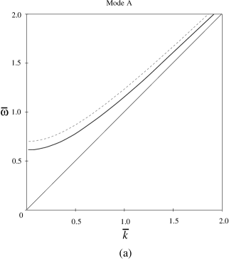
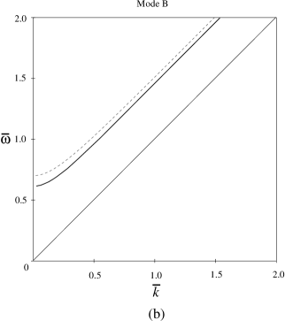
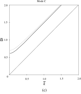
FIG. 3.: The dispersion relations for the modes A, B and C in units of $\left(16\pi G\rho\right)^{1/2}$ for real frequencies and wave vectors. The dashed lines stand for the leading $T^{4}$ contributions and the full lines represent the inclusion of the $T^{2}$ sub-leading corrections for $G\,T^{2}=0.01$. The light-cone is represented by the diagonal.

FIG. 4.: The source-ghost Feynman diagram. The full/wave line on the left represents the external source.

REFERENCES

- [1] D. I. Gross, M. J. Perry, and L. G. Yaffe, Phys. Rev. D 25, 330 (1982); Y. Kikuchi, T. Moriya, and T. Tsukahara, Phys. Rev. D 29, 2220 (1984).
- [2] P. S. Gribosky, J. F. Donoghue, and B. R. Holstein, Ann. Phys. (N.Y.) 190, 149 (1989).
- [3] R. Kobes, G. Kunstatter and A. Rebhan, Nucl. Phys. B355, 1 (1991).
- [4] A. Rebhan, Nucl. Phys. B351, 706 (1991).
- [5] J. Frenkel and J. C. Taylor, Z. Phys. C 49, 515 (1991); F. T. Brandt, J. Frenkel, and J. C. Taylor, Nucl. Phys. B374, 169 (1992); F. T. Brandt and J. Frenkel, Phys. Rev. D 48, 4940 (1993).
- [6] A. P. de Almeida, F. T. Brandt and J. Frenkel, Phys. Rev. D 49, 4196 (1994).
- [7] U. Kraemmer and A. Rebhan, Phys. Rev. Lett 67, 793 (1991); H. Nachbagauer, A. K. Rebhan and D. J. Schwarz, Phys. Rev. D 53, 882 (1996); H. Nachbagauer, A. K. Rebhan, D. J. Schwarz, Phys. Rev. D 53 5468 (1996).
- [8] P.F. Kelly, Q. Liu, C. Lucchesi and C. Manuel, Phys. Rev. D50, 4209 (1994).
- [9] F. T. Brandt, J. Frenkel, and J. C. Taylor, Nucl. Phys. B437, 433 (1995).
- [10] F. T. Brandt and J. Frenkel, Phys. Rev. D 47, 4688 (1993).
- [11] J. I. Kapusta, Thermal Field Theory (Cambridge University Press, Cambridge, England 1996).
- [12] H. A. Weldon, hep-ph/9701279.
- [13] J. I. Kapusta, Finite Temperature Field Theory (Cambridge University Press, Cambridge, England 1989).
- [14] G. Barton, Ann. of Phys. (N.Y.) 200 (1990) 271; J. Frenkel and J. C. Taylor, Nucl. Phys. B374, 156 (1992).
- [15] F. T. Brandt and J. Frenkel, Phys. Rev. D 56, 2453 (1997).
- [16] R. Delbourgo and T. Matsuki, Phys. Rev. D 23, 2579 (1985).
- [17] F. T. Brandt, J. Frenkel and J. C. Taylor Phys. Rev. D 50, 4110 (1994).
- [18] F. T. Brandt, J. Frenkel and J. C. Taylor Phys. Rev. D 55, 7808 (1997).
- [19] F. T. Brandt, J. Frenkel, Phys. Rev. Lett. D 74, 1705 (1995).
- [20] G. ´t Hooft and M. Veltman, Ann. Inst. Henri Poincaré 20, 69 (1974).
- [21] N. H. Barth and S. M. Christensen, Phys. Rev. D 28, 1876 (1983).