LBNL-41466, UCB-PTH-98/13

hep-th/9803050

Matrix Description of Intersecting M5 Branes
Shamit Kachru, Yaron Oz and Zheng Yin

Department of Physics, University of California at Berkeley
366 Le Conte Hall, Berkeley, CA 94720-7300, U.S.A.
and
Theoretical Physics Group, Mail Stop 50A–5101
Ernest Orlando Lawrence Berkeley National Laboratory,
Berkeley, CA 94720, U.S.A.

Novel 3+1 dimensional ${\cal N}=2$ superconformal field theories (with tensionless BPS string solitons) are believed to arise when two sets of M5 branes intersect over a 3+1 dimensional hyperplane. We derive a DLCQ description of these theories as supersymmetric quantum mechanics on the Higgs branch of suitable 4d ${\cal N}=1$ supersymmetric gauge theories. Our formulation allows us to determine the scaling dimensions of certain chiral primary operators in the conformal field theories. We also discuss general criteria for quantum mechanical DLCQ descriptions of supersymmetric field theories (and the resulting multiplicities and scaling dimensions of chiral primary operators).

1 Introduction

Many new nontrivial RG fixed points of supersymmetric field theories in various dimensions have been discovered in recent years. A host of novel fixed points in 3,4,5, and 6 dimensions were discovered using string theory arguments. For many of these theories, there is no known ultraviolet Lagrangian which flows to them in the infrared. Therefore, it is of interest to find other ways of defining them, that do not involve all of the degrees of freedom of string or M theory.

For some of the simplest novel fixed points in six dimensions, with $(2,0)$ and $(1,0)$ supersymmetry, such an alternative definition has been proposed in [1, 2, 3, 4]. In analogy with the matrix model for M theory [5, 6], it was proposed that the discrete light-cone quantization (DLCQ) of these 6d field theories can be formulated in terms of a suitable supersymmetric quantum mechanics. A similar description of 4d ${\cal N}=4$ Super Yang-Mills was discussed in [7]. In this paper, we initiate the study of matrix descriptions for 4d theories with 8 supercharges, by providing an analogous DLCQ description of a class of ${\cal N}=2$ superconformal fixed points. These 3+1 dimensional fixed points govern the physics on the intersection of $K$ M5 branes intersecting $K^{\prime}$ M5 branes along a 3+1 dimensional hyperplane. The two sets of M5 branes can be connected by membranes which give rise to BPS saturated tensionless strings on the intersection. Such intersections were discussed, for instance, in [8].

In the next section, we present the brane configuration which gives rise to the ${\cal N}=2$ fixed points and specify the decoupling limit (in which the physics on the brane intersection should be expected to decouple from gravity). We construct a Matrix description of this system, by studying the quantum mechanics of $N$ D0 branes in the background of intersecting D4 branes. The zero brane quantum mechanics reduces to a sigma model on the Higgs branch of a 4d ${\cal N}=1$ supersymmetric gauge theory. In §3 we study the structure of the Higgs branch for general $K,K^{\prime}$ and provide arguments for the decoupling. We find that the quantum mechanics has a branch localized on the intersection which decouples from the “bulk” in the limit of §2. In §4 we analyze quantum mechanical states that correspond to chiral primary operators of the 4d superconformal theory. These states come from compact cohomology representatives localized at the origin of the Higgs branch, as in [11]. By computing this cohomology, we are able to provide the multiplicities and scaling dimensions of certain chiral primary operators in the conformal field theory. In §5 we discuss general criteria for a Matrix description of supersymmetric field theories, and make some general remarks about the resulting multiplicities and scaling dimensions of chiral primary operators. In §6, we summarize the main points and discuss relations with other recent work on the DLCQ description of field theories.

2 The Target and Its Probe

2.1 The Target: A Theory of Tensionless Strings

We start in M theory with a number of M5 branes, whose worldvolume configurations can be divided into two types that we label as M5 and M5’ in table 1. There are $K$ and $K^{\prime}$ of them respectively.

Table 1: Configurations of the branes in M theory

	0	1	2	3	4	5	6	7	8	9	10
M5	$\times$	$\times$	$\times$	$\times$	$\times$						$\times$
M5’	$\times$	$\times$	$\times$			$\times$	$\times$				$\times$

Such a configuration can preserve up to 8 supercharges, corresponding to ${\cal N}$=2 in 4d. Of the original $Spin(1,10)$ Lorentz symmetry, only the (1+3)d Lorentz group, $SL(2,{C})$, of the 0, 1, 2, and 10th directions and the Euclidean rotation group $SU(2)_{789}\times U(1)_{34}\times U(1)_{56}$ remain manifest. From the usual rule for branes ending on branes [9, 10], we know that there can be open membranes ending on and stretched in between the two types of M5-branes. They look like strings in the (1+3)d common directions and have tension $M_{pl}^{3}l$. We are interested in the limit

$$M_{pl}\rightarrow\infty$$ (2.1)

and

$$M_{pl}^{3}l={\rm fixed},$$ (2.2)

where $l$ is the distance between the two sets of M5 branes in the 7-8-9 directions. In this double scaling limit, the bulk gravity decouples from the M5 branes while the tension of the BPS strings mentioned above remains constant. Our particular interest is in the limit when the two sets of M5 branes coincide, and the BPS strings become tensionless. One might expect a theory with tensionless string solitons to be nontrivial. It is known that the decoupled theory on two parallel and coincident M5-branes is interacting [1, 2], and we expect that the configuration in table 1 also yields interacting fixed points. What is a priori not obvious is whether the tensionless strings in this case are a feature of an intrinsic 3+1 dimensional theory, localized at the intersection and decoupled from the “bulk” of the two types of M5 branes. In latter sections we will present evidence in support of this.

We can compactify the 10th direction on a circle and go to type IIA string theory. The resulting configuration is that of two sets of D4-branes, as summarized in table 2.

Table 2: Configurations of the branes in IIA

	0	1	2	3	4	5	6	7	8	9
D4	$\times$	$\times$	$\times$	$\times$	$\times$
D4’	$\times$	$\times$	$\times$			$\times$	$\times$

The strings from open membranes can be either wrapped around the 10th direction or transverse to it in the M theory picture. In the IIA picture these two kinds of configurations give rise to particles from open strings and strings from open D2-branes. The particles make up $K\times K^{\prime}$ hypermultiplets. In the limit (eq. 2.2), they are massless. We shall label the scalars in them and their VEVs as $\theta_{a}^{a\prime}$ and $\tilde{\theta}^{a}_{a\prime}$, $K\times K^{\prime}$ and $K^{\prime}\times K$ matrices respectively.

2.2 The Probe

As usual it is very difficult to analyze this interacting system using conventional field theory techniques. To this end we take the DLCQ approach of [1, 2, 11]. After the procedures outlined in [12, 13], the physics of the N momentum sector is described by N D0-branes probing the configuration of table 2. The DLCQ procedure breaks the $SL(2,{C})$ Lorentz group of table 1 down to $U(1)_{12}$. This combined system now has 4 supercharges, equivalent to ${\cal N}$=1 supersymmetry in 4d reduced to quantum mechanics. The transformation properties of the holomorphic supercharges $\cal Q$ and the superpotential are given in table 3. To find the lightest fields of the quantum mechanics and their interactions, we consider first the D0 brane probes alone and then introduce the two types of D4-branes.

Table 3: Transformation property of the supercharges and superpotential

	$U(1)_{12}$	$U(1)_{34}$	$U(1)_{56}$	$SU(2)_{789}$
$\cal Q$	+1	+1	+1	(2)
$W$	+2	+2	+2	(1)

From the D0-branes themselves, we have the content of an ${\cal N}$=4 D=4 vector multiplet dimensionally reduced to quantum mechanics. This breaks down to one ${\cal N}$=1 D=4 vector multiplet and 3 chiral multiplets in the adjoint. In total there are 9 scalars, $\Phi^{i}$, $i=1\ldots 9$, parameterizing the transverse fluctuation of the D0-brane. The scalars in the vector multiplet in the quantum mechanics are $\Phi^{7},\Phi^{8},\Phi^{9}$ (in the language of the dimensional reduction, they come from Wilson lines of the gauge field around the $T^{3}$). The other scalars come from the dimensional reduction of the 3 chiral multiplets. We write their holomorphic combinations as $\Phi_{12}$, $\Phi_{34}$, and $\Phi_{56}$ respectively. There is a superpotential

$$W_{PP}=tr\Phi_{12}\mbox{$\left[\Phi_{34},\Phi_{56}\right]$}.$$

The subsystem consisting of the probes and the unprimed D4-branes supports 8 supercharges, dimensionally reduced from ${\cal N}$=2 in 4d. In addition to the fields described above, we also have $K$ hypermultiplets in the fundamental of $U(N)$, coming from open strings starting on the D0 branes and ending the D4 branes. They decomposes under the supersymmetry in table 3 into chiral multiplets $Q$ and $\tilde{Q}$ with $a=1\ldots K$. This system has a superpotential

$$W_{PA}=\sum_{a}Q\Phi_{56}\tilde{Q}.$$ (2.3)

Similarly for the subsystem consisting of the probes and the primed D4-branes, we obtain chiral multiplets $Q^{\prime}$ and $\tilde{Q}^{\prime}$ with $a^{\prime}=1\ldots K^{\prime}$ and a superpotential

$$W_{PB}=\sum_{a\prime}Q^{\prime}\Phi_{34}\tilde{Q}^{\prime}.$$ (2.4)

To summarize, the fields, parameters and R charges in the quantum mechanical theory are as follows:

Table 4: Fields of the Quantum Mechanics

	$U(1)_{12}$	$U(1)_{34}$	$U(1)_{56}$	$SU(2)_{789}$
$\Phi_{12}$	+2	0	0	(1)
$\Phi_{34}$	0	+2	0	(1)
$\Phi_{56}$	0	0	+2	(1)
$Q,\tilde{Q}$	$+1$	+1	0	(1)
$Q^{\prime},\tilde{Q}^{\prime}$	+1	0	+1	(1)
$\Phi_{789}$	0	0	0	(3)

In keeping with the usual matrix approach, VEVs of fields in the target (D4-brane) theory becomes parameters in the probe quantum mechanics. The obvious ones are the diagonal VEVs for the scalars in the adjoint of $U(K)$ and $U(K^{\prime})$ from the two sets of D4-branes, which we will call $X$ and $X^{\prime}$ respectively. They are mass parameters and can be shifted to zero for the configuration satisfying (eq. 2.2). Then there are the VEVs for the hypermultiplets $\theta$ and $\tilde{\theta}$, as well as backgrounds for antisymmetric 3-form tensor field strengths $H$ and $H^{\prime}$ on the two types of M5-branes. The latter map to Fayet-Iliopoulos parameters in the quantum mechanics, as in [11]. For the model under consideration here, the FI parameters split into real parameters $\zeta_{R}$ and $\zeta^{\prime}_{R}$ as well as complex parameters $\zeta_{C}$ and $\zeta^{\prime}_{C}$. In addition to these parameters, there is also the coupling constant $g$ for the D0-brane gauge theory. It is given by

$$g^{2}=(RM_{pl}^{2})^{3}$$ (2.5)

where $R$ is the radius of the DLCQ circle. $g$ has mass dimension $\frac{3}{2}$. The limit (eq. 2.1) implies that $g\rightarrow\infty$ and therefore we are interested in the infrared (i.e. large time) limit of the probe quantum mechanics. Unlike the gauge coupling for ${\cal N}$=1 supersymmetric gauge theories in 4d, the gauge coupling $g$ is not part of a background field that is charged under the $U(1)$ global symmetries. The transformation properties of all these parameters are given in table 5.

Table 5: Parameters of the Quantum Mechanics

	$U(1)_{12}$	$U(1)_{34}$	$U(1)_{56}$	$SU(2)_{789}$
$\zeta_{{R}}$	0	0	0	(1)
$\zeta_{A}$	+2	+2	0	(1)
$\zeta_{B}$	+2	0	+2	(1)
$\theta,\tilde{\theta}$	0	+1	+1	(1)

By the usual supersymmetric nonrenormalization theorem, $g$ can only appear in the superpotential through nonperturbative effects. Since $g$ carries no charges under any global symmetry, there is no other restriction on it. From this table and from the analysis in [11] on the backgrounds for the antisymmetric tensor field strengths, one finds that the following types of (schematically written) couplings are present the tree-level superpotential:

$$W_{poss}=\zeta_{C}{\mbox{$\mathrm{tr}$}}\Phi_{56}+\zeta^{\prime}_{C}{\mbox{$\mathrm{tr}$}}\Phi_{34}+\theta_{a}^{a^{\prime}}Q^{\prime}\tilde{Q}+\tilde{\theta}^{a}_{a\prime}Q_{a}\tilde{Q}^{\prime}+{\mbox{$\mathrm{tr}$}}\Phi_{12}\theta_{a}^{a^{\prime}}\tilde{\theta}^{a}_{a\prime}$$ (2.6)

It is clear that nonvanishing $\theta$ and $\tilde{\theta}$ will give masses to the quarks as well as $\Phi_{12}$. In fact, the interacting theory that we are interested in studying occurs at the origin of parameter space, where all of the parameters in $W_{poss}$ should be set to zero. However, we will at present keep the $\zeta_{C}$ and $\zeta^{\prime}_{C}$ terms and explain why we cannot turn them on (even as a regulator [11]) later in the paper. The complete superpotential is therefore

$$W = W_{PP}+W_{PA}+W_{PB}$$ (2.7)

$$= {\mbox{$\mathrm{tr}$}}\Phi_{12}\mbox{$\left[\Phi_{34},\Phi_{56}\right]$}+{\mbox{$\mathrm{tr}$}}Q\Phi_{56}\tilde{Q}+\zeta_{C}{\mbox{$\mathrm{tr}$}}\Phi_{56}+{\mbox{$\mathrm{tr}$}}Q^{\prime}\Phi_{34}\tilde{Q}^{\prime}+\zeta^{\prime}_{C}{\mbox{$\mathrm{tr}$}}\Phi_{34}.$$

An important question is whether (2.7) is exact. The symmetries in table 4 show that all the terms which can be constructed from integer powers of the fields are already included in (2.7). One might worry about the possibility of negative or fractional powers. At large VEVs for $\Phi_{34}$ or $\Phi_{56}$ we should get the instanton moduli space as the moduli space of vacua. This suggests that terms with negative or fractional powers of the fields are absent.

3 The Target Space of the Probe

In the limit that gravity decouples from the brane theory in spacetime, the coupling constant of the DLCQ quantum mechanics becomes infinite. This corresponds to its infrared (large time) limit, and the D0 brane theory flows to a supersymmetric $\sigma$-model quantum mechanics. Its target space is simply the moduli space of flat directions determined by the usual D-term and F-term equations. Understanding the geometry and topology of this space is an important step in obtaining useful information about the spacetime theory of tensionless strings using the Matrix probes.

The target space for the quantum mechanics described in the previous section possesses very rich structures, not all of which are relevant to us. Some parts of the moduli space describe the probes away from the two types of D4-branes; other parts describe the probes as instantons in some of the D4-branes. The only relevant region for us is the one in which all the probes are stuck at the (1+2)d intersection. However, ${\it a~{}priori~{}}$ the D0-brane probes are free to wander into other regions of the moduli space. In this section we analyze the relevant branch of the moduli space and try to address this important issue of decoupling. First we review the arguments for decoupling of the $(2,0)$ theory, which has been studied extensively in the literature. The probe theory for that case has 8 supercharges. The branch of interest, where the D0-branes are probing the interior of the D4-branes, is the Higgs branch of the moduli space and enjoys strong nonrenormalization properties that shield its metric from radiative corrections. Our model is much more complicated, and is not protected by such powerful nonrenormalization theorems. Still, many similarities to the (2,0) case exist, and after analyzing the geometry of the moduli space we will be able to propose and verify a decoupling criterion.

3.1 A Lesson from the (2,0) Theory

The quantum mechanics which arises in the DLCQ description of (2,0) theories is a dimensional reduction of $U(N)$ SYM in 4d with ${\cal N}$=2 supersymmetry. The theory includes $K$ fundamental hypermultiplets (where $K$ is the number of D4 branes being probed), and an additional adjoint hypermultiplet. The F term equations look like

$$\mbox{$\left[\Phi_{12},\Phi_{34}\right]$}+\tilde{Q}Q=\zeta_{A};$$ (3.1)

$$\mbox{$\left[\Phi_{12},\Phi\right]$}=0=\mbox{$\left[\Phi_{34},\Phi\right]$};$$ (3.2)

$$\Phi\tilde{Q}=0=Q\Phi;$$ (3.3)

$Q$ is a $K\times N$ matrix, $\tilde{Q}$ is $N\times K$.

The D-term equations for the 4d gauge theory are

$$\mbox{$\left[\Phi_{12},\Phi_{12}^{\dagger}\right]$}+\mbox{$\left[\Phi_{34},\Phi_{34}^{\dagger}\right]$}+\mbox{$\left[\Phi,\Phi^{\dagger}\right]$}+$$

$$QQ^{\dagger}-\tilde{Q}^{{\dagger}}\tilde{Q} = \zeta_{R}.$$ (3.4)

where $\zeta_{R}$ here is the sum of the contribution from the two types of D4-branes.

To understand the structure of the moduli space of vacua, we consider solutions to these equations. We will discuss the 4d gauge theory (i.e. the 3 brane - 7 brane system instead of the 0 brane - 4 brane system), and then abstract lessons for the quantum mechanics at the end. As is well known, the D-term equation combined with the $U(N)$ quotient is equivalent to a quotient by $GL(N;C)$ of the holomorphic field variables. Therefore we only need to study the solution to the F-term equations quotiented by $GL(N;C)$. For generic values of $\Phi$, it is a nondegenerate $N\times N$ complex matrix. (eq. 3.3) implies that $Q$ and $\tilde{Q}$ both vanish — they become massive. Also, a generic matrix $\Phi$ has distinct eigenvalues. The rest of the F-term equations then imply that we can simultaneously diagonalize $\Phi_{12}$, $\Phi_{34}$ and $\Phi$ to use up all of the $GL(N;C)$ except for a $(C^{*})^{N}$ factor, which represents the complexification of the unbroken $U(1)^{N}$ gauge symmetry and the $S_{N}$ Weyl group. This is the Coulomb phase, the moduli space is that for the adjoint scalar in the vector multiplet $\Phi$ times that for the diagonal adjoint hypermultiplet. The $\Phi$ branch receives quantum corrections to its metric from integrating out the $Q$s and $\tilde{Q}s$ and develops a logarithmic “throat,” while the branch parameterized by the adjoint hyper retains its classical $R^{4N}$ metric.

Another branch can be found by letting, say, $\tilde{Q}$ be generic. As it turns out, we can also allow, say, $\Phi_{12}$ to be generic. For $K\geq N$, genericity of $\tilde{Q}$ already forces $\Phi$ to be zero (i.e. it is massive). For $K<N$, this is insufficient by itself. However, (eq. 3.2) imposes a condition on $\Phi$. For a generic value of $\Phi_{12}$, we can choose a basis in which $\Phi$ and $\Phi_{12}$ can be simultaneously diagonalized. In this basis, it is easy to see that (eq. 3.3) cannot be satisfied for generic $\tilde{Q}$ unless $\Phi$ vanishes. To make this more explicit, (eq. 3.2) and (eq. 3.3) imply that

$$\Phi\exp^{\alpha\Phi_{12}}\tilde{Q}=0$$ (3.5)

for arbitrary $\alpha$. Therefore the $K$ $N$-vectors in $Q$ are in a $\Phi_{12}$ invariant proper subspace of $C^{N}$ unless $\Phi$ vanishes. Thus genericity of $Q$ implies the vanishing of $\Phi$. After setting $\Phi$ to $0$, the rest of the F-term equations can be satisfied, yielding a moduli space of complex dimension $2NK$ that is birational to a symmetric product [2]. This is a branch parameterized purely by scalars in the hypermultiplets, a maximally Higgsed branch. It is in fact equivalent to the moduli space of $N$ $U(K)$ instantons.

The above two branches are connected at a region where $Q$, $\tilde{Q}$, and $\Phi$ all vanish. This is where all the instantons are of zero size but still attached. The metric diverges as one travels from the interior of the Coulomb branch to this point, due to radiative corrections at one loop from virtual quarks. On the other hand, the metric from the interior of the hypermultiplet branch to the origin of $Q$ and $\tilde{Q}$ and in varying $\Phi_{12}$ and $\Phi_{34}$ is uncorrected and remains finite. There are also mixed branches, corresponding to non-generic but nonvanishing values of $\Phi$. When $\Phi$ has rank $n<N$, for example, the solutions to the F-term equations give a branch which corresponds to $n$ instantons and $N-n$ detached D3-branes. All these branches are also separated from each other by “tubes ” along which the metric for $\Phi$ develops similar divergences.

The divergence in the metric persists if we dimensionally reduce this theory to $d<4$ dimensions. The divergence of the metric takes the form $\frac{1}{r^{4-d}}$, while for $d=4$ the tube metric diverged only logarithmically. Therefore at $d=2$ and lower the divergence will result in an infinitely long tube. This is very important because in $d\leq 2$, physical states are described by wavefunctions spread out over the flat directions, and only an infinitely long tube can decouple wavefunctions in different regions of the moduli space. In using the D0-branes to probe the D4-branes as in [1, 2, 11], it was a necessary sign of consistency that the maximally Higgsed branch is separated from the mixed and Coulomb branches by such infinite tubes. Otherwise, the D0-brane physics could not be used as a definition of an intrinsic theory on the M5-branes that is believed to decouple from the bulk of spacetime.

In our theory, we will face a similar test of consistency, but the reduced supersymmetry allows a moduli space that is far more intricate. Because the analysis of decoupling of the utmost importance, and yet the quantum mechanics for our model is complicated, it is useful to develop a set of criteria based on the much better understood case of instantons. Ideally, fluctuations along the flat directions that move the D0 branes away from the branch of interest should be massive. The mass is typically of the form $g\phi$, where $g$ is the gauge coupling constant and $\phi$ is the VEV that leads to the mass. In the limit we take, $g\rightarrow\infty$ as $M_{pl}\rightarrow\infty$, so the mass actually becomes infinite. The scalar potential that is responsible for giving masses to potential moduli takes the form

$$L_{scalar}=\sum_{i}{\left|F_{i}\right|}^{2}$$ (3.6)

where $F_{i}$ are the F-terms. Therefore massless fluctuations correspond to the kernel of the matrix

$$M_{ij}=\frac{{\partial}F_{i}}{{\partial}\phi_{j}},$$ (3.7)

where the $\phi$s are chiral multiplets of the theory. In other words, they are solutions to the linearized F-term equations.

At special subloci on the Higgs branch of interest in our case, additional fields become massless and the Higgs branch intersects partial Coulomb branches. At such points, the decoupling argument will break down unless the metric on the (partial) Coulomb branch has an infinite tube due to a loop correction to its metric. In theories with 8 supercharges, the metric perturbatively receives at most one-loop corrections. However, in the case we study, the reduced supersymmetry allows higher loops to contribute in general and no general results about perturbatively exact metrics are known. Nevertheless, our model strongly resembles the Matrix description of the (2,0) theory. In particular, the superpotential is obtained as a sum of contributions from different 0-4 subsectors, which each have 8 supercharges. At the one loop level, we can determine whether there is a divergence in the metric by comparing with the theories of [1]. If there is a divergence at one-loop, it is unlikely to be removed by higher loops and/or nonperturbative effects.

The divergence in the metric generated at one-loop originates from virtual massive charged particles running in the loop. Therefore, if along some flat direction the number of charged massless particles decreases, then we expect a divergent one-loop renormalization of the metric along that branch. In other words, for some solution of

$$M_{ij}\delta_{1}\phi_{j}=0\mskip 6.0mu,$$ (3.8)

that corresponds to a charged particle, there is no solution for $\delta_{\epsilon}\phi$ to the first order perturbation equation

$$\frac{{\partial}M_{ij}}{{\partial}\phi_{k}}\delta_{2}\phi_{k}\delta_{1}\phi_{j}+M_{ij}\delta_{\epsilon}\phi=0,$$ (3.9)

where $\delta_{2}\phi$ is the flat direction away from the region of interest. In our case $\delta_{1}\phi_{j}$ is the flat direction along the branch parameterized by $Q,\tilde{Q}$ while $\delta_{2}\phi_{j}$ is the flat direction along the branch parameterized by $\Phi_{34}$ and $\Phi_{56}$. Since by (eq. 3.7)

$$\frac{{\partial}M_{ij}}{{\partial}\phi_{k}}=\frac{{\partial}M_{ik}}{{\partial}\phi_{j}}.$$

(eq. 3.9) is equivalent to

$$\frac{{\partial}M_{ij}}{{\partial}\phi_{k}}\delta_{1}\phi_{k}\delta_{2}\phi_{j}+M_{ij}\delta_{\epsilon}\phi=0.$$ (3.10)

In other words, this fluctuation $\delta_{2}\phi$ also become massive as one turns on $\delta_{1}\phi$. This is precisely what happens at the origin of the Higgs branch for the theory of eight supercharges. Of course, this is only a necessary condition for the said flat direction to grow an infinitely long tube. One has to directly check that the loop graphs including the relevant F-terms lead to a divergent metric.

3.2 The Intersecting Fivebrane Quantum Mechanics

The F-term equations derived from the superpotential (eq. 2.7) are

$$\mbox{$\left[\Phi_{12},\Phi_{34}\right]$}+\tilde{Q}Q = 0;$$ (3.11)

$$\mbox{$\left[\Phi_{12},\Phi_{56}\right]$}+\tilde{Q}^{\prime}Q_{\prime} = 0;$$ (3.12)

$$\Phi_{56}\tilde{Q}= 0 =Q\Phi_{56};$$ (3.13)

$$\Phi_{34}\tilde{Q}^{\prime}= 0 =Q^{\prime}\Phi_{34};$$ (3.14)

$$\mbox{$\left[\Phi_{34},\Phi_{56}\right]$}=0$$ (3.16)

Since we want the D0-branes to probe the theory at the intersection, we want to set $\Phi_{34}$ and $\Phi_{56}$ to $0$. The reduced F-term equations for the moduli space of interest are

$$\mbox{$\left[\Phi_{12},\Phi_{34}\right]$}+\tilde{Q}Q = 0;$$ (3.17)

$$\mbox{$\left[\Phi_{12},\Phi_{56}\right]$}+\tilde{Q}^{\prime}Q^{\prime} = 0;$$ (3.18)

$$\Phi_{34}=0=\Phi_{56}.$$ (3.19)

There is no condition on $\Phi_{12}$.

These equations immediately imply that for $N>1$, we cannot turn on the complex Fayet-Iliopoulos terms if $N>\max(K,K^{\prime})$. Otherwise, the RHS of (eq. 3.11) would be replaced by a nonvanishing multiple of the identity. Then, the RHS would have greater rank than the maximum possible for the LHS and there is no solution. Intuitively, a complex Fayet-Iliopoulos term forces the instantons to spread out on the D4-brane they are associated with in all directions, which directly conflicts with confining the D0-branes in the intersection. This is in stark contrast to the $(2,0)$ model analyzed in [11]. However, the real Fayet-Iliopoulos terms are still compatible with our solution. We will use them to resolve certain singularities, and analyze the compact cohomology of the (partially desingularized) resultant space, as in [11]. We will return to this point later on.

The solution space to the matrix equation $\tilde{Q}Q=0$ has a series of branches, labeled by an integer $\lambda=rank(Q)$ ranging from $\max(0,K-N)$ to $\min(N,K)$ inclusive, with dimensions

$$NK+\lambda K-\lambda^{2}.$$ (3.20)

The total space is quite complicated, with these different branches emanating from positive codimensional submanifolds. It is unlikely that the branches are separated by an infinite distance. A similar structure exists in the instanton moduli spaces which arise in the DLCQ definition of the (2,0) theories, and there all of these branches must be included. We study the details of this space in the following subsections for different values of $K$, $K^{\prime}$, and $N$.

To find the total dimension of the moduli space after quotienting by $GL(N;C)$, we diagonalize $\Phi_{12}$. The eigenvalues of $\Phi_{12}$ then contribute $N$ to the dimension of the moduli space. Adding the contributions of the particular branch we choose for the $Q$ and $\tilde{Q}$ VEVs and the $Q^{\prime}$ and $\tilde{Q}^{\prime}$ VEVs, and finally taking into account the quotient by the remaining $C^{*}$s, the dimension of the branch characterized by $(r={{\mbox{$\mathrm{Rank}$}}}(Q),r^{\prime}={{\mbox{$\mathrm{Rank}$}}}(Q^{\prime}))$ is

$$N+(NK+rK-r^{2})+(NK^{\prime}+r^{\prime}K^{\prime}-r^{\prime 2})-N=N(K+K^{\prime})+r(K-r)+r^{\prime}(K-r^{\prime}).$$ (3.21)

As we shall discuss in the next section, for a Matrix quantum mechanical model to have the usual DLCQ probe interpretation, the cohomology of its moduli space should exhibit the properties of a symmetric product. The simplest way this can happen is if the moduli space itself is a symmetric product. This however turns out not to be true in our case and the moduli space is not a symmetric product. We shall comment on this as we analyze the moduli space for the appropriate case and return for a more elaborate discussion in the next section.

To justify the constraint (eq. 3.19) we also need to analyze the solutions to the linearized F-term equations with $\Phi_{34}$ and $\Phi_{56}$ set to zero:

$$\mbox{$\left[\Phi_{12},\delta\Phi_{34}\right]$}+\delta\tilde{Q}Q+\tilde{Q}\delta Q = 0;$$ (3.22)

$$\mbox{$\left[\Phi_{12},\delta\Phi_{56}\right]$}+\delta\tilde{Q}^{\prime}Q^{\prime}+\tilde{Q}^{\prime}\delta Q^{\prime} = 0;$$ (3.23)

$$\delta\Phi_{56}\tilde{Q}= 0 =Q\delta\Phi_{56};$$ (3.24)

$$\delta\Phi_{34}\tilde{Q}^{\prime}= 0 =Q^{\prime}\delta\Phi_{34}.$$ (3.25)

3.2.1 $K=K^{\prime}=1$

Let us first consider the simplest case, $K=K^{\prime}=1$. The equation for $\tilde{Q}_{i}Q^{j}$ has two branch of solutions: one in which $Q=0$ but $\tilde{Q}$ is arbitrary, and the converse. The same is true for $Q^{\prime}$ and $\tilde{Q}^{\prime}$. $\Phi_{12}$ is arbitrary. We must now take into account the ${GL(N,C)}$ quotient. Generically, we can diagonalize $\Phi_{12}$. This gauge-fixes ${GL(N,C)}$ up to a residual ${C^{*}}^{N}\Join S_{N}$, where $\Join$ denotes a semi-direct product and $S_{N}$ is the N-th order permutation group.

To gauge-fix the residual symmetry, we consider the four branches of solutions to (eq. 3.17) as in table 6.

Table 6: Four branches of solutions to (eq. 3.17) for $K=K^{\prime}=1$

Branch		$Q=0=\tilde{Q}^{\prime}$	$\tilde{Q}=0=Q^{\prime}$ $Q=0=Q^{\prime}$	$\tilde{Q}=0=\tilde{Q}^{\prime}$
After Quotient	$({C})^{N}$	$({C})^{N}$	origin	origin

Each $C^{*}$ factor of the residual symmetry group acts on a pair of primed and unprimed quarks. If one is tilded and the other untilded, then $C^{*}$ acts instead as, for example,

$$(Q,\tilde{Q}^{\prime})\rightarrow(\lambda Q,\frac{1}{\lambda}Q^{\prime})$$

and the quotient is still noncompact and simply $C^{1}$, parameterized by $Q\tilde{Q}^{\prime}$. If they are of the same type, (both tilded or both untilded) then $C^{*}$ acts as, for example,

$$(Q,Q^{\prime})\rightarrow(\lambda Q,\lambda Q^{\prime}).$$

Naively, the result of this quotient is a ${\bf CP}^{1}$ with the pair as the homogeneous coordinates. However, there is a subtlety. In [15], where the D-flatness condition with vanishing real Fayet-Iliopoulos term is considered, it was found that the $C^{*}$ quotients must be taken in a generalized sense so that, in the present context, the whole ${\bf CP}^{1}$ is collapsed to and identified with the point at the origin ($Q=\tilde{Q}=Q^{\prime}=\tilde{Q}^{\prime}=0)$. Finally we take into account of the $S_{N}$ action. This just replaces the direct products in table 6 by symmetric products. Therefore the moduli space looks like figure 1.

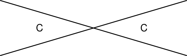
Figure 1: Moduli space for $K=K^{\prime}=1$, $\zeta=0$

It consists of two cones, each a symmetric product of $N$ ${C}$’s. If one turns on $\zeta_{R}$, the situation becomes subtler still. Now one of the two branches on the right in table 6 is lifted completely while the other become a compact space, replacing the origin. For $N=1$, the compact space is a ${\bf CP}^{1}$ and the moduli space looks like figure 2 The size of the sphere is controlled by $\zeta_{R}$. Note that the sphere still touches the two $C$s at a point.

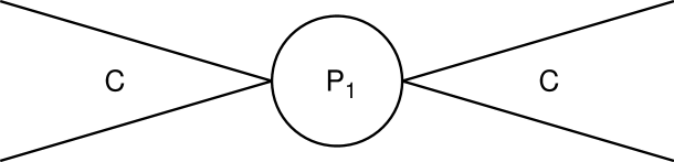
Figure 2: Moduli space for $K=K^{\prime}=1=N$, $\zeta\neq 0$

For higher $N$, the sphere is replaced by some other complex N manifold.

Now we shall justify imposing the constraint (eq. 3.19) by demonstrating decoupling in the manner outlined earlier. The same argument works for all four branches and for both $\Phi_{34}$ and $\Phi_{56}$, so for definiteness we take $Q=0=Q^{\prime}$, $\tilde{Q}$ and $\tilde{Q}^{\prime}$ arbitrary, and concentrate on $\Phi_{34}$. The relevant linearized F-term equation is

$$\Phi_{34}\delta\tilde{Q}^{\prime}=0.$$ (3.26)

Let us diagonalize $\Phi_{34}$ and look at (eq. 3.22), which specializes to

$$\mbox{$\left[\Phi_{12},\delta\Phi_{34}\right]$}+\tilde{Q}\delta Q=0.$$ (3.27)

The commutator’s diagonal elements are all zero. Generically $\tilde{Q}$ is a column N-vector with all nonvanishing entries. The two together imply that

$$\delta Q=0,$$

which means $\delta\Phi_{34}$ must commute with $\Phi_{12}$, an arbitrary $N\times N$ matrix. As shown earlier, this together with (eq. 3.26) imposes a condition on $\Phi_{12}$ and $\tilde{Q}^{\prime}$ that is not satisfied generically. For nongeneric $\Phi_{12}$ and $\tilde{Q}$ that does support a solution to (eq. 3.26) and (eq. 3.27), the same argument as in the case of the (2,0) theory suggests that there is an infinite tube along the flat direction of $\Phi_{34}$ and completes the decoupling argument.

3.2.2 General Case — Moduli Space

The analysis of the moduli space for higher $K$ and $K^{\prime}$ proceeds in a similar vein, but becomes very complicated. First of all, the solution space to $\tilde{Q}Q=0$ now consists of more than two branches. The additional possibility is for $Q$ and $\tilde{Q}$ nonvanishing. As one would expect from 4d ${\cal N}$=1 theories, the structure changes drastically for $N$ greater or less than $K$ and/or $K^{\prime}$. Perhaps more surprisingly, the discussion of decoupling also depends on $N$. There may be a spacetime connection between the two. We take this as a suggestion that for the theories we study here the probe reflects the chiral primary spectrum of the spacetime theory only in the large N limit, contrary to the case studied in [11].

$K\geq K^{\prime}\geq N$

Once $K$ and/or $K^{\prime}$ is greater than $1$, the solution to (eq. 3.17) becomes complicated, as explained in the paragraph following that equation. When $N<K\leq K^{\prime}$, the space of solutions does not contain any symmetric product. To see this, consider for illustration the equation $\tilde{Q}Q=0$ and think of $Q$ and $\tilde{Q}$ each as $N$ $K$-vectors grouped together. Because $N<K$, both $Q$ and $\tilde{Q}$ can be simultaneously nonvanishing in any branch. Generically in each branch, the space can be thought of as the solution for $\tilde{Q}$ fibered over a matrix $Q$ of certain rank or the converse. The fiber is nontrivial and become singular (enlarged) at certain submanifolds of the base. It is this fibration structure that prevents the total space from becoming a symmetric product after taking the $S_{N}$ quotient. For $K<N$, this fiber is nontrivial in every branch.

On the other hand, the decoupling of $\Phi_{34}$ and $\Phi_{56}$ is straightforward. The genericity of $Q$ and $\tilde{Q}$, for instance, in each branch is sufficient to force both $\Phi_{56}$ and $\delta\Phi_{56}$ to vanish through (eq. 3.13), because together they form $K\geq N$ linearly independent $N$-vectors. The arguments given earlier show that at nongeneric values of $Q$ and $\tilde{Q}$, the flat direction along $\Phi_{56}$ is an infinitely long tube. Similar arguments apply to $\Phi_{34}$. However, despite the decoupling, the spacetime interpretation of such cases is not clear, because of the lack of a symmetric product structure. It is possible that for this model we should only expect the usual spacetime interpretation to hold at sufficiently large N, while for smaller N some peculiarity of the DLCQ becomes significant and obscures the spacetime physics.

$N>K\geq K^{\prime}$

For $N\geq K$, there are branches in the solution space to $\tilde{Q}Q=0$ where either $Q$ or $\tilde{Q}$ is constrained to be zero. The case $K=1$ treated earlier is a special case of this type. These are the branches in which the fibration structure discussed above become trivial. Therefore, as discussed earlier, the whole moduli space will have components that are symmetric products after taking care of the quotient. Because this is the appropriate structure for a spacetime interpretation, we shall concentrate on these components. The whole analysis parallels that for $K=K^{\prime}=1$ and we shall be brief.

These well behaved branches again decompose into four components. They and their quotient by $(C^{*})^{N}$ have a similar classification to the one we found in table 6, as shown in table 7.

Table 7: Four branches of solutions to (eq. 3.17) for $K=K^{\prime}=1$

Branch	$Q=0=\tilde{Q}^{\prime}$	$\tilde{Q}=0=Q^{\prime}$	$Q=0=Q^{\prime}$	$\tilde{Q}=0=\tilde{Q}^{\prime}$
After Quotient	$({C}^{K+K^{\prime}-1})^{N}$	$({C}^{K+K^{\prime}-1})^{N}$	origin	origin

After $\zeta_{R}$ is turned on, a compact space emerges and replaces the origin in similar fashion to what happens for $K=K^{\prime}=1$.

The decoupling analysis also becomes more involved. (eq. 3.13) by itself can force neither $\Phi_{56}$ nor $\Phi_{34}$ to be zero even generically, because the quarks do not have sufficient rank. As in the $K=K^{\prime}=1$ case, one has to use (eq. 3.22). Let us concentrate on $\Phi_{34}$ and the branch in which $Q=0$. (eq. 3.22) reduces to

$$\mbox{$\left[\Phi_{12},\delta\Phi_{34}\right]$}=-\tilde{Q}\delta Q.$$ (3.28)

This time $\tilde{Q}\delta Q$ does not necessarily vanish. However, because $K<N$, the RHS has only rank K and is not generic and is constrained by the value of $\tilde{Q}$. The LHS, however, depends only on $\Phi_{12}$, $Q^{\prime}$, and $\tilde{Q}^{\prime}$ – the latter two through

$$\delta\Phi_{34}\tilde{Q}^{\prime}=0=Q^{\prime}\delta\Phi_{34}.$$ (3.29)

From (eq. 3.17) and (eq. 3.19), we see there is no correlation between them. Therefore generically there is no solution to (eq. 3.28). The same applies to $\Phi_{56}$.

$K>N>K^{\prime}$

For values of $N$ in this range, the moduli space is a mixture of the two types we analyzed above. The solution space for $Q^{\prime}$ and $\tilde{Q}^{\prime}$ has components that are N-th order symmetric products, while that for $Q$ and $\tilde{Q}$ does not. Since $S_{N}$ acts simultaneously on primed and unprimed quarks, the total space does not have the structure of a symmetric product.

The analysis of decoupling for these cases is even more intricate. While (eq. 3.24) forces $\delta\Phi_{56}$ to vanish, it only forces $\delta\Phi_{34}$ to have rank no more than $N-K^{\prime}$. Does (eq. 3.22) impose any constraint? At least in some branches of moduli space the answer is no. Consider the one in which the rank of $Q$ is $N$. Then for arbitrary $\delta\Phi_{34}$, there is a solution to (eq. 3.22) for $\delta\tilde{Q}$ because $Q$ is invertible in an appropriate sense. $K\geq N$ is crucial here. For other branches the situation is more complicated and it appears at least for some of them (eq. 3.22) imposes a very weak constraint on $\delta\Phi_{34}$. Nonetheless for these values of $N$, the problems in at least one part of the Higgs branch strongly suggest a difficulty with decoupling.

4 Moduli space and chiral primary operators

In previous sections, we have developed a quantum mechanical matrix description of the four dimensional ${\cal N}=2$ superconformal theory on the intersection of $K$ and $K^{\prime}$ fivebranes. In this section, we use this quantum mechanics to compute the dimensions of some of the chiral primary operators in the CFT with tensionless strings.

The target space of the quantum mechanics describing the theory on the intersection of the branes has singularities of various codimensions. We resolve them by using the FI parameters. We have two sets of FI parameters $(\zeta_{R},\zeta_{C})$ and $(\zeta_{R}^{\prime},\zeta_{C}^{\prime})$. As in [11] the space-time interpretation of the FI parameters involves turning on constant self dual 3-form field strength $H,H^{\prime}$ on the two sets of fivebranes. We have $(\zeta_{R},\zeta_{C})\sim H_{+ij},i,j=1,2,3,4$ and $(\zeta_{R}^{\prime},\zeta_{C}^{\prime})\sim H_{+ij}^{\prime},i,j=1,2,5,6$.

Turning on the real FI parameters corresponds to a resolution of singularities. Turning on the complex FI parameters corresponds to a deformation. We argued in the previous section that in order to have a consistent space time interpretation of the theory we have to set $\zeta_{C}=\zeta_{C}^{\prime}=0$. We will further elaborate on this point later. The superconformal field theory that we study arises when the FI parameters vanish. As in [11] we consider the large time behaviour of the quantum mechanics where the finite FI parameter can be absorbed by a wave function renormalization of the operators. This provides a procedure to relate the quantum mechanical wave functions at finite FI parameters to the states of the SCFT.

We will study the chiral primary operators of the four dimensional theory that correspond to the compact cohomology of the resolved moduli space of the quantum mechanics localized at the origin [11]. The localization at the origin is a consequence of the general fact that a quantum mechanical state which corresponds to a primary operator is localized at the origin of the moduli space [11], and this will play an important role in the analysis. This state may be viewed as a particular representative of the compact cohomology which is obtained by scaling of a compact cohomology representative which is not concentrated at the origin.

The space-time dimension $D$ of a chiral primary operator corresponding to a form $O$ with compact support of degree $deg(O)$ is

$$D=deg(O)-\frac{1}{2}dim_{R}({\cal M}^{res}_{N;K,K^{\prime}})\mskip 6.0mu.$$ (4.1)

${\cal M}^{res}_{N;K,K^{\prime}}$ is the resolved moduli space.

4.1 The case $K=1,K^{\prime}=1$

Consider the system with $(K=1,K^{\prime}=1)$. The moduli space ${\cal M}_{N;1,1}$ has complex dimension $2N$. It has the structure of a product of $C^{N}$ with the $N$ complex dimensional space constructed from two copies of $C^{N}/S_{N}$ intersecting at the origin.

We will first analyze the momentum one case $N=1$. The moduli space ${\cal M}_{1;1,1}=C\times{\cal M}_{1;1,1}^{0}$ has complex dimension two. ${\cal M}_{1;1,1}^{0}$ is parameterized by the complex coordinates $A=Q{\tilde{Q}}^{\prime},B=Q^{\prime}{\tilde{Q}}^{\prime}$ and has the structure of two complex planes intersecting at the origin as in figure 1. Therefore the origin is a singular point. Note for comparison that in the $(2,0)$ field theory on $k$ parallel fivebranes studied in [11] the $k=1,N=1$ moduli space is $R^{4}$ which does not have a singularity. Turning on the real FI parameter $\zeta_{R}$ changes ${\cal M}_{1;1,1}^{0}$ to the space of figure 2. This does not resolve the singularity at the origin but rather shifts its location to two points. In order to resolve the singularity at the origin we have to deform it using a complex FI parameter $\zeta_{C}$. However the singularity at the origin is part of the physics that one D0 brane probes, and a deformation of this singularity will change the physics of the system.

Consider the compact cohomology of ${\cal M}_{1;1,1}^{0}$ scaled to be localized at the origin. Obviously we have the top 2-form localized at the origin. The question is whether we have something else. Although there is a 0-form on the $CP^{1}$ connecting the two complex planes in figure 2, it cannot be extended to a 0-form on the whole ${\cal M}_{1;1,1}^{0}$. The reason is that its extension would have to be a constant and the moduli space is noncompact. We could also try to consider the top 2-form on each of the complex planes or on the $CP^{1}$ separately. However such a compact cohomology element has to vanish on the points of intersection of the complex planes and the $CP^{1}$, which means that is vanishes as $\zeta_{R}\rightarrow 0$. Therefore such candidate forms cannot represent wave functions localized at the origin.

To summarize, the compact cohomology localized at the origin of ${\cal M}_{1;1,1}$ consists of only the top 4-form which is the wedge product of the top form of $C$ and the top form of ${\cal M}_{1;1,1}^{0}$. The top 4-form localized at the origin corresponds to a chiral primary operator $O$ of the four dimensional theory. Using (4.1) the dimension of the operator $O$ is two. The fact that we have a dimension two operator implies that the space time theory is a non-trivial ${\cal N}=2$ SCFT. The operator $O$ is part of the ${\cal N}=2$ chiral ring at the point where the string becomes tensionless. This can be contrasted with the case of one fivebrane. In this case the analysis of the compact cohomology in [11] shows that there is one operator of dimension 2 in six dimensions and the theory is free. Our case resembles more the case of $k=2$ fivebranes in [11]. In that case there is also a tensionless string and the theory is not free in the IR.

Consider next the momentum two case $N=2$. The moduli space ${\cal M}_{2;1,1}=C^{2}\times{\cal M}_{2;1,1}^{0}$ has complex dimension four. ${\cal M}_{2;1,1}^{0}$ consists of two copies of $C^{2}/S_{2}$ intersecting at the origin. The analysis is similar to the $N=1$ case. Turning on $\zeta_{R}\neq 0$ connects the two $C^{2}/S_{2}$ spaces by a compact space. Primary operators correspond to quantum mechanical states localized at the origin. In order to describe chiral primary operators we will consider compact cohomologies on each of the components of ${\cal M}_{2;1,1}^{0}$ and scale them to the origin. We cannot consider compact cohomologies on each of the components separately since we will have to require that they vanish on the intersections which at $\zeta_{R}\rightarrow 0$ implies that they vanish at the origin. Therefore we get a compact cohomology class corresponding to the resolution of the orbifold singularity of the two $C^{2}/S_{2}$. It gives a 6-form on ${\cal M}_{2;1,1}$ which we scale to be localized at the origin. We also have the top 8-form which we can localize at the origin. Thus we get using (4.1) two operators of dimensions two and four. The interpretation of the result is clear: at $N=2$ we expect to see $O(1/R)^{2}$ and $O(2/R)$ which are of dimensions four and two respectively.

The generalization to arbitrary momentum $N$ is straightforward. The moduli space ${\cal M}_{N;1,1}=C^{N}\times{\cal M}_{N;1,1}^{0}$ where ${\cal M}_{N;1,1}^{0}$ consists of two copies of $C^{N}/S_{N}$ intersecting at the origin. Turning on $\zeta_{R}\neq 0$ connects the two $C^{N}/S_{N}$ spaces by a compact space. In order to describe chiral primary operators we will consider compact cohomologies on each of the components of ${\cal M}_{N;1,1}^{0}$ and scale them to the origin. Again, we cannot consider compact cohomologies on each of the components separately since we will have to require that they vanish on the intersections which at $\zeta_{R}\rightarrow 0$ implies that they vanish at the origin. Thus, we find that the number of chiral primary operators of dimension $2k$ is

$$b_{2k}=p_{k}(N),~{}~{}~{}~{}~{}~{}~{}~{}k=1,...,N\mskip 6.0mu,$$ (4.2)

where $p_{k}(N)$ is the number of partitions of $N$ to $k$ parts. Note that a consistency check on our analysis is the fact that we do not get operators with negative dimensions. The result is compatible with the fact that at momentum $N$ we expect to see operators that are products of $O$ at momenta $p_{-}=k_{i}/R$, namely $O(k_{1}/R)\cdots O(k_{r}/R)$ where $\sum k_{i}=N$.

If we deform ${\cal M}_{N;1,1}$ using the complex FI parameters then at $N=1$ we get $AB=\zeta_{C}$, and compact cohomology of the deformed ${\cal M}_{1;1,1}^{def}$ localized at the origin consists of a 3-form and a 4-form. Using (4.1) the dimension of the corresponding chiral primary operators $\Psi,O$ are one and two respectively. However for higher $N$ we lose the symmetric product structure and the the analysis of the compact cohomology localized at the origin is not compatible with a space-time interpretation. This is in agreement with the fact that turning on $\zeta_{C}$ forces the probes to spread out off of the intersection, and should therefore not correspond to a spacetime deformation of the 3+1 dimensional theory.

So, we see that requiring a family of quantum mechanical systems to be the DLCQ description of a space time theory is very stringent. It requires that the appropriate compact cohomologies scaled to the origin have the dimensions of classes arising from the resolution of orbifold singularities of a symmetric product target space. In our case, where the moduli space had two components intersecting at the origin, this implied that we should not resolve the singularity at the origin.

4.2 The general $K,K^{\prime}$ case

Consider now the general system with arbitrary numbers of fivebranes $(K,K^{\prime})$. The structure of the moduli space ${\cal M}_{N;K,K^{\prime}}$ has been analyzed in section 3. It has several branches of different dimensions. One of the branches has complex dimension $N(K+K^{\prime})$ and its structure is a direct generalization of that in the case $K=K^{\prime}=1$. It has the structure of a product of $C^{N}$ with the the $N(K+K^{\prime}-1)$ complex dimensional space constructed from two copies of $C^{N(K+K^{\prime}-1)}/S_{N}$ intersecting at the origin. Again, the real FI parameter resolves the singularities of the symmetric products and connects the two $C^{N(K+K^{\prime}-1)}/S_{N}$ spaces by a compact space . The other branches have various dimensions that depend on an integer parameter $\lambda$ and do not have the form of a symmetric product.

As before we want to consider quantum mechanical states that are localized at the origin. In the case $K=K^{\prime}=1$ we considered compact cohomologies scaled to the origin. This led us to consider only those compact cohomologies that arise from the resolution of the symmetric product singularities and the top form. All other possibilities of compact cohomologies (localized on one of the two resolved $C^{N}/S_{N}$s or on the compact space arising in the $\zeta_{R}\neq 0$ case) vanish upon scaling to the origin. Applying the same strategy here we are led to consider only the compact cohomology classes which arise from the resolution of symmetric product singularities on the branch of complex dimension $N(K+K^{\prime}-1)$.

Consider first the momentum one case $N=1$. The moduli space ${\cal M}_{1,K,K^{\prime}}=C\times{\cal M}_{1;K,K^{\prime}}^{0}$ has complex dimension $K+K^{\prime}$, where ${\cal M}_{1;K,K^{\prime}}^{0}$ has the structure of two copies of $C^{K+K^{\prime}-1}$ intersecting at the origin. Turning on $\zeta_{R}\neq 0$ connects the two $C^{K+K^{\prime}-1}$ spaces by a compact space. Again, in order to describe chiral primary operators we will consider compact cohomologies on each of the components of ${\cal M}_{1;K,K^{\prime}}^{0}$ and scale them to the origin. We cannot consider compact cohomologies on each of the components separately since we will have to require that they vanish on the intersections which at $\zeta_{R}\rightarrow 0$ implies that they vanish at the origin. Therefore we get only the $2(K+K^{\prime})$ top form of ${\cal M}_{1;K,K^{\prime}}$ localized at the origin. It corresponds to a chiral primary operator $O$ of the four dimensional theory of dimension $K+K^{\prime}$.

The generalization to arbitrary momentum $N$ is straightforward. We look for compact cohomologies localized at the origin. Only those that arise from the resolution of the symmetric product singularities are relevant. We get that the number of chiral primary operators of dimension $k(K+K^{\prime})$ is $p_{k}(N),k=1,...,N$. As guaranteed by the procedure the result is compatible with the fact that at momentum $N$ we expect to see operators that are products of $O$ at momenta $p_{-}=k_{i}/R$, namely $O(k_{1}/R)\cdots O(k_{r}/R)$ where $\sum k_{i}=N$.

5 General moduli space

An interesting question that naturally arises is the following: Given supersymmetric quantum mechanics on a moduli space ${\cal M}_{N;\vec{k}}$ where $\vec{k}$ stands for a set of parameters $\vec{k}=\{k_{1},...k_{n}\}$ what are the necessary and sufficient conditions to have a space time interpretation of the model in the DLCQ sense. In the following we will discuss necessary conditions on the cohomology with compact support (and localized at the origin).

In general we tend to expect that ${\cal M}_{N;\vec{k}}$ is birational to the symmetric product of ${\cal M}_{1;\vec{k}}$

$${\cal M}_{N;\vec{k}}\simeq Sym^{N}{\cal M}_{1;\vec{k}}\mskip 6.0mu,$$ (5.1)

namely they are equivalent up to the singularities. The physical reason behind this is the fact that $N$ D0 branes probing the space-time theory see the $N$-th product of the moduli space seen by one D0 brane, up to permutation. However, in the examples that we studied in previous sections we saw that this is not necessarily the case. The physics of N D0 probes can sometimes involves couplings that do not vanish even if we separate them.

The real requirement involves the compact cohomology localized at the origin, which corresponds to chiral primary operators. In the case that $M_{N;\vec{k}}$ satisfies (5.1) these correspond to the compact cohomology of the resolved space. Let us proceed with this case and discuss the more subtle case later. Consider ${\cal M}_{1;\vec{k}}$ and let $d$ be the complex dimension of $M_{1;\vec{k}}$. Since the compact cohomologies of $M_{N;\vec{k}}$ correspond to chiral primary operators in the space time theory with dimensions given by (4.1), and these dimensions must be non-negative, we have as a second requirement that the compact cohomologies satisfy

$${\rm dim}H^{p}(M_{1;\vec{k}}) = 0~{}~{}~{}~{}~{}~{}p=0,...,d-1$$

$${\rm dim}H^{p}(M_{1;\vec{k}}) = b_{p}~{}~{}~{}~{}~{}~{}p=d,...,2d\mskip 6.0mu,$$ (5.2)

where $b_{p}$ can be different than zero.

Consider now general $N$. We expect that the chiral primary operators that we see at momentum $N$, which we get from the compact cohomology of ${\cal M}_{N;\vec{k}}$, are just products of the operators $O_{i}$ at momenta $p_{-}=k_{i}/R$, namely $O_{i}(k_{1}/R)\cdots O_{r}(k_{r}/R)$ where $\sum k_{i}=N$. Using this fact and (5.2) we can derive the generating formula for the dimensions of the compact cohomologies

$$\prod_{l=1}^{\infty}\prod_{i=d}^{2d}\left(1-(-1)^{i}t^{i+d(l-1)}q^{l}\right)^{-(-1)^{i}b_{i}}=\sum_{p,N}{\rm dim}H^{p}({\cal M}_{N;\vec{k}})t^{p}q^{N}\mskip 6.0mu.$$ (5.3)

This is the third requirement. Note that due to (5.2) we have ${\rm dim}H^{p}({\cal M}_{N;\vec{k}})=0,p<Nd$.

In (5.3) we considered the general case with both odd and even cohomologies. The moduli space that we studied in previous sections (as well as the moduli space of $k$ $U(N)$ instantons) has only even cohomology classes. Note that when the cohomology is odd (even) we have the corresponding term in (5.3) in the numerator (denominator). The interpretation of this in the quantum mechanics is that while the chiral primary operators corresponding to even cohomologies have bose statistics, those that correspond to odd cohomologies have odd statistics. Thus, for instance $O(k/R)O(k/R)=0$ if $O$ corresponds to an odd-dimensional cohomology class.

When the moduli space does not satisfy (5.1) the above discussion holds provided in (5.2) and (5.3) we replace ${\rm dim}H^{p}({\cal M}_{N;\vec{k}})$ by the compact cohomology localized at the origin, as discussed in previous sections.

6 Discussion

Our results suggest that there is a decoupled theory living on the 3+1 dimensional intersection of groups of $K$ and $K^{\prime}$ M5 branes. The part of the chiral ring we are able to identify with the cohomology of the Higgs branch seems to be generated by a single chiral operator, of dimension $K+K^{\prime}$. This might seem surprising in view of the fact that the (2,0) theory living on $K$ coincident M5 branes has a spectrum of independent chiral operators that grows with $K$ [11]. However, in that case the field theory has a moduli space $R^{5k}/S_{k}$ (along which one separates the $K$ M5 branes) and the states in the quantum mechanics have a natural interpretation as functions on this moduli space. In contrast, in our case separating one of the $K$ (or $K^{\prime}$) M5 branes from the rest is related to a field theory mode supported on the full $K$ ($K^{\prime}$) M5 brane theory, and does not correspond to an excitation which is localized on the intersection. Presumably, only motion of the center of mass of the $K$ M5 branes away from the $K^{\prime}$ M5 branes is related to a state in the decoupled quantum mechanics. This is the state created by an operator of dimension $K+K^{\prime}$.

In the DLCQ description of the e.g. (2,0) field theory [1], decoupling was obvious for every momentum sector, even for small values of $N$. In contrast, here we find that only for $N$ large enough (compared to $K$ and $K^{\prime}$) can one make a decoupling argument. Similarly, in the (2,0) case the moduli space ${\cal M}_{N,k}$ was (birational to) a symmetric product $({\cal M}_{1,k})^{N}/S_{N}$. In our case the moduli space for generic $K,K^{\prime}$ is not a symmetric product. However, at large $N$ the $\it cohomology$ of this space, which is related to chiral operators in spacetime, does look like that of a symmetric product. Since the DLCQ is really only “supposed” to be related to the higher-dimensional field theory at large $N$, this is not unacceptable.

Recently, problems which arise in the DLCQ of 4d field theories (due to strongly coupled zero modes) were discussed in [16]. Our description, like analogous descriptions of other field theories derived using D0 brane probes in string theory, does not obviously suffer from these problems (in much the same way that the D0 brane quantum mechanics of M(atrix) theory does not suffer from the problems a direct DLCQ of 11d supergravity would). Nevertheless, the difficulties we encounter at low values of $N$ may be somehow related to the issues discussed in [16].

Finally, we should note that recently it has been proposed (and to some extent verified) that one may use supergravity as a master field to solve certain conformal field theories which arise on branes, if the supergravity solution is known [17]. However, for the case of intersecting branes (or branes ending on other branes), the appropriate (localized) supergravity solutions are not yet available. Therefore, the DLCQ approach is still the primary tool we currently have for investigating these theories.

References

- [1] O. Aharony, M. Berkooz, S. Kachru, N. Seiberg, and E. Silverstein, “Matrix Description of Interacting Theories in Six Dimensions,” hep-th/9707079.
- [2] E. Witten, “The Conformal Field Theory of the Higgs Branch,” hep-th/9707093.
- [3] D. Lowe, “ Small Instantons in Matrix Theory,” hep-th/9709015.
- [4] O. Aharony, M. Berkooz, S. Kachru and E. Silverstein, “Matrix Description of (1,0) Theories in Six Dimensions,” hep-th/9709118.
- [5] T. Banks, W. Fischler, S. Shenker and L. Susskind, “M theory as a Matrix Model: A Conjecture,” Phys. Rev. D55 (1997) 112, hep-th/9610043.
- [6] L. Susskind, “Another Conjecture about Matrix Theory,” hep-th/9704080.
- [7] O. Ganor and S. Sethi, “New Perspectives on Yang-Mills Theories with Sixteen Supersymmetries,” hep-th/9712071.
- [8] A. Hanany and I. Klebanov, “Tensionless Strings in 3+1 Dimensions,” Nucl. Phys. B482 (1996) 105, hep-th/9606136.
- [9] A. Strominger, “Open P-Branes,” Phys.Lett. B383 (1996) 44, hep-th/9512059.
- [10] P.K. Townsend, “Brane Surgery,” Nucl. Phys. Proc. Suppl. 58 (1997) 163, hep-th/9609217.
- [11] O. Aharony, M. Berkooz and N. Seiberg, “Light-Cone Description of (2,0) Superconformal Theories in Six Dimensions,” hep-th/9712117.
- [12] N. Seiberg, “Why is the Matrix Model Correct?” Phys.Rev.Lett. 79 (1997) 3577, hep-th/9710009.
- [13] A. Sen, “D0 Branes on and Matrix Theory,” hep-th/9709220.
- [14] O. Aharony, A. Hanany, K. Intriligator, N. Seiberg, M.J. Strassler, “Aspects of Supersymmetric Gauge Theories in Three Dimensions,” Nucl.Phys. B499 (1997) 67, hep-th/9703110.
- [15] M. A. Luty, W. Taylor, “Varieties of vacua in classical supersymmetric gauge theories,” Phys.Rev. D53 (1996) 3399, hep-th/9506098.
- [16] S. Hellerman and J. Polchinski, “Compactification in the Lightlike Limit,” hep-th/9711037.
- [17] J. Maldacena, “The Large N Limit of Superconformal Field Theories and Supergravity,” hep-th/9711200.