FSUJ-TPI-98/03

DIAS-STP-98/02

February 1998

hep-th 9802191

Monopoles, Polyakov-Loops and Gauge Fixing on the Torus

C. Ford, U. G. Mitreuter, T. Tok, A. Wipf
Theor.–Phys. Institut, Universität Jena
Fröbelstieg 1, D–07743 Jena, Germany

J. M.  Pawlowski
Dublin Institute for Advanced Studies,
10 Burlington Road, Dublin 4, Ireland

We consider pure Yang Mills theory on the four torus. A set of non-Abelian transition functions is presented which encompass all instanton sectors. It is argued that these transition functions are a convenient starting point for gauge fixing. In particular, we give an extended Abelian projection with respect to the Polyakov loop, where $A_{0}$ is independent of time and in the Cartan subalgebra. In the non-perturbative sectors such gauge fixings are necessarily singular. These singularities can be restricted to Dirac strings joining monopole and anti-monopole like “defects”.

1 Introduction

A long standing and yet unsolved problem is to explain color confinement in QCD. An important first step in this direction would be to prove the confinement of static quarks. Indeed, this has been convincingly demonstrated by many lattice studies [1]. However, it would be desirable to study this phenomenon with less reliance on numerics, since Monte Carlo simulations do not have the logical transparency of mathematical derivations. The relevant observables are products of Wilson-loop operators [2]. When one has periodicity in Euclidean time (ie. finite temperature) then one may use a Polyakov loop [3] operator, ie. the Polyakov loop is a closed, periodic time-like Wilson loop.

Since the Lagrangian includes massless fields and one is interested in the infrared behaviour of the theory, it is sensible to implement some kind of infrared cutoff. It is well-known for example that in supersymmetric theories with massless modes, the non-renormalisation “theorems” fail in the absence of an infrared regulator [4]. One possibility is to use a Wilsonian effective action [5] which by definition includes a momentum space infrared cut-off on the quantum fluctuations. An alternative procedure is to simply work on some compact Euclidean space. Of these, the four torus, $T^{4}$, is the most attractive. When dealing with $T^{4}$, one automatically includes the finite temperature case ($S^{1}\times\mbox{l}\!\mbox{R}^{3}$), and unphysical curvature effects are absent. On $T^{4}$ one also maintains translational invariance, and thus any relevant supersymmetry.

We assume that our gauge fields are periodic in time

$$\begin{array}[]{rcl}\displaystyle A_{\mu}(x^{0}+\beta,\vec{x})=A_{\mu}(x_{0},\vec{x}).\end{array}$$ (1.2)

In the quantum theory, we may interpret $\beta$ as the inverse temperature, see for example [6]. The Polyakov loop operator $P(\vec{x})$ is defined as the following trace of a path ordered exponential of $A_{0}$

$$P(\vec{x})=\mbox{Tr}~{}\Gamma\left({\cal P}(\beta,\vec{x})\right),\quad\hbox{{where}}\quad{\cal P}(x^{0},\vec{x})={\cal P}\exp\left[i\int^{x^{0}}_{0}d\tau A_{0}(\tau,\vec{x})\right],$$

and $\Gamma$ is the representation of the gauge group which acts on the fermions. The Polyakov loop is invariant under gauge transformations which are periodic in time. The two-point function

$$e^{-\beta F(\vec{x},\vec{y})}=\langle P(\vec{x})P^{\dagger}(\vec{y})\rangle_{\beta}$$

yields the free energy $F(\vec{x},\vec{y})$ in the presence of a heavy quark at $\vec{x}$ and a heavy antiquark at $\vec{y}$. In the confining low-temperature phase $F(\vec{x},\vec{y})$ increases for large separations of the quark-antiquark pair and thus $\langle P(\vec{x})P^{\dagger}(\vec{y})\rangle\to 0$. In the deconfining high-temperature phase the free energy reaches a constant value for large separations and $\langle P(\vec{x})P^{\dagger}(\vec{y})\rangle\to\hbox{constant}\neq 0$. Inferring the cluster property we see that $\langle P\rangle_{\beta}$ vanishes in the confining phase but not in the deconfining one. In other words, it is an order parameter for confinement.

Note that the Weyl gauge, $A_{0}=0$, is not compatible with time-periodicity. Yet we still would like $A_{0}$ to be as simple as possible, since we are interested in observables only depending on $A_{0}$. On the two dimensional torus, $T^{2}$, one can perform an Abelian projection [7] with respect to the Polyakov loop operators and gauge fix in such a way that $A_{0}$ is in the Cartan subalgebra and is independent of time, while preserving the time periodicity of $A_{1}$. In this gauge one has a remarkable cancellation between part of $\exp(-S)$ and the Fadeev-Popov determinant. This simplifies the calculation of the partition function and the expectation value of the Polyakov loop order parameter, and avoids zero mode ambiguities [8].

In this paper we address the question of to what extent the gauge fixing used in [8] can be generalised to QCD on the four torus. The gauge fixing procedure hinges on the diagonalisation of the path ordered exponential, ${\cal P}(\beta,\vec{x})$, whose trace is the Polyakov loop. It is convenient that ${\cal P}(\beta,\vec{x})$ be periodic in the spatial variables. Yet unless we are in the perturbative sector, the gauge fields themselves are necessarily non-periodic. This non periodicity is characterised by a set of group-valued transition functions. We introduce a set of non-Abelian transition functions which facilitate a periodic ${\cal P}(\beta,\vec{x})$ even in the non-perturbative sectors. Unlike the well known Abelian transition functions introduced by ’t Hooft [9], our transition functions encompass all instanton sectors, thus solving the problem of finding smooth transition functions for the odd instanton sectors of $SU(2)$ gauge theory.

In contrast to the two dimensional case the diagonalisation procedure has unavoidable singularities. The singularities can be interpreted as Dirac strings [10] joining magnetically charged “defects”. Here we understand defects as points, loops (not to be confused with the Dirac strings!), sheets and lumps where ${\cal P}(\beta,\vec{x})$ has degenerate eigenvalues. The locations of the defects are gauge invariant and may be viewed as additional “collective coordinates” associated to the gauge fixing. The simplest case (and probably the most relevant for the QCD path integral) is where one only has point defects (which can be viewed as magnetic monopoles). Here the final gauge fixed potential has very simple periodicity properties, and the topological charge is completely fixed by the network of monopoles and Dirac strings (see also [11]). We also consider the more general case where one has extended defects.

The outline of this paper is as follows. In section two we recall some basic facts about gauge fields on the torus, including the standard Abelian transition functions. Our new set of non-Abelian transition functions (which includes the odd sector of $SU(2)$) is presented in section 3. We also explain how one can use the Polyakov loop itself to define a different set of non-Abelian transition functions. Next, in section 4 we elaborate our gauge fixing procedure, and study the special case where one has no defects. In section 5 we discuss the problem of defects, and show how they contribute to the instanton number. Conventions and some technical results are collected in three appendices.

2 Gauge fields on $T^{4}$

We view the four torus as $\mbox{l}\!\mbox{R}^{4}$ modulo the lattice generated by four orthogonal vectors $b_{\mu},\quad\mu=0,1,2,3$. The Euclidean lengths of the $b_{\mu}$ are denoted by $L_{\mu}$ (we may identify $L_{0}$ with the inverse temperature $\beta$). Local gauge invariants such as $\hbox{Tr}F_{\mu\nu}F_{\mu\nu}$ are periodic with respect to a shift by an arbitrary lattice vector. However, it follows that gauge fields have to be periodic only up to gauge transformations. In order to specify boundary conditions for gauge potentials $A_{\alpha}$ on the torus one introduces a set of transition functions $U_{\mu}(x)$, which are defined on the whole of $\mbox{l}\!\mbox{R}^{4}$. The periodicity properties of $A_{\alpha}$ are as follows

$$\begin{array}[]{rcl}\displaystyle A_{\alpha}(x+b_{\mu})=U_{\mu}^{-1}(x)A_{\alpha}(x)U_{\mu}(x)+iU_{\mu}^{-1}(x)\partial_{\alpha}U_{\mu}(x),\quad\mu=0,1,2,3\end{array}$$ (2.2)

where the summation convention is not applied. The transition functions $U_{\mu}(x)$ have to satisfy the cocycle condition

$$U_{\mu}(x)U_{\nu}(x+b_{\mu})=U_{\nu}(x)U_{\mu}(x+b_{\nu}).$$

Under a gauge transformation, $V(x)$, the pair $(A,U)$ is mapped to

$$A_{\alpha}^{V}(x)=V^{-1}(x)A_{\alpha}(x)V(x)+iV^{-1}(x)\partial_{\alpha}V(x),\ \ \ U_{\mu}^{V}(x)=V^{-1}(x)U_{\mu}(x)V(x+b_{\mu}).$$

We define the (integer valued) topological charge or instanton number as follows

$$q={1\over 32\pi^{2}}\int_{T^{4}}\epsilon_{\mu\nu\alpha\beta}\hbox{Tr}\,F_{\mu\nu}F_{\alpha\beta}.$$

The integrand in (LABEL:topological) can be written as a total derivative. Using Stokes theorem we get

$$q = \frac{1}{24\pi^{2}}\sum_{\mu}\int_{{\cal B}_{\mu}}\epsilon_{\mu\nu\rho\sigma}\mbox{Tr}\left[(U^{-1}_{\mu}\partial_{\nu}U_{\mu})(U^{-1}_{\mu}\partial_{\rho}U_{\mu})(U^{-1}_{\mu}\partial_{\sigma}U_{\mu})\right]$$

$$-\frac{1}{8\pi^{2}}\sum_{\mu,\nu}\int_{{\cal B}_{\mu\nu}}\epsilon_{\mu\nu\rho\sigma}\hbox{Tr}\left[(U^{-1}_{\nu}\partial_{\rho}U_{\nu})(\partial_{\sigma}U_{\mu}(x+b_{\nu})U^{-1}_{\mu}(x+b_{\nu}))\right],$$

with

$${\cal B}_{\mu}=\{x\in T^{4}|x_{\mu}=0\},\qquad{\cal B}_{\mu\nu}=\{x\in T^{4}|x_{\mu}=x_{\nu}=0\}.$$

(see also [12]). That is $q$ is fully determined by the transition functions. In particular, if we take all the transition functions to be the identity (i.e. we assume the gauge fields are periodic in all directions) then the instanton number is zero. Accordingly, if we are to describe the non-perturbative sectors, one must consider non-trivial transition functions. For a given $q$ we only require one set of transition functions. If we have two sets of transition functions with the same instanton number then they are gauge equivalent [12].

For $SU(N)$, $N>2$, one can write down a set of very simple Abelian transition functions, which include all possible values of $q$. For $SU(2)$, the situation is rather peculiar, in that there exist Abelian transition functions for the even instanton number case, but for odd $q$, the transition functions are necessarily non-Abelian.

Consider the following set of transition functions

$$U_{0}=U_{2}=1\!\mbox{l},\quad U_{1}(x)=e^{2\pi iH_{1}\xi_{2}},\quad U_{3}(x)=e^{2\pi iH_{3}\xi_{0}},$$

where $H_{1},H_{3}\in{\cal L}$, with ${\cal L}$ being the discrete lattice in the Cartan subalgebra ${\cal H}$;

$${\cal L}\equiv\left\{H\in{\cal H}|e^{2\pi iH}=1\!\mbox{l}\right\}$$

and we have introduced the dimensionless coordinates

$$\begin{array}[]{rcl}\displaystyle\xi_{\mu}=x_{\mu}/L_{\mu},\quad\mu=0,1,2,3.\end{array}$$ (2.10)

These transition functions satisfy the cocycle condition (LABEL:cocycle), and using (LABEL:q), the instanton number associated with these transition functions is simply

$$q=\mbox{Tr}\,H_{1}H_{3}.$$

Now, if we take $H_{3}$ to be proportional to $H_{1}$ it is easy to see that $q$ is always even. To get an odd charge one must take non-parallel $H$’s. For example, in $SU(3)$ consider

$$H_{1}=\left(\begin{array}[]{ccc}\displaystyle 1&0&0\\ 0&-1&0\\ 0&0&0\end{array}\right)\quad\hbox{ and }\quad H_{3}=\left(\begin{array}[]{ccc}\displaystyle 0&0&0\\ 0&-1&0\\ 0&0&1\end{array}\right).$$

In this case $q=1$. However, for $SU(2)$ $H_{1}$ and $H_{3}$ must be parallel since the Cartan subalgebra is one dimensional. Hence, within this class of transition functions one is restricted to even topological charges. Although the transition functions (LABEL:trans) are not the most general Abelian transition functions, it is easy to see that any Abelian transition functions lead to an even $q$ for $SU(2)$.

Although we have concentrated on the transition function question, another (to date unsolved) problem is to obtain the instantons for pure gauge theory on $T^{4}$. While ’t Hooft found some extremely simple “Abelian” instantons [9], these can only represent single points in the moduli space of a given instanton sector. This is in sharp contrast to the situation on $S^{4}$ where Atiyah et al [13] gave an algebraic recipe for computing all instantons. In fact one of the few things known about instantons on $T^{4}$ is a negative result. Using the Nahm transformation [14], van Baal [15] has argued that there are no $SU(N)$ instantons with $q=1$. We should stress that while there are no charge one instantons there do exist configurations with $q=1$. While for $q=1$, the minimal action is never achieved one can find configurations whose action is arbitrarily close to the instanton number. Numerical [16] and analytical studies indicate that as one brings the action closer to the minimum the action density becomes concentrated near a point. For the higher charge $|q|>1$ sectors, smooth instantons are known to exist [17]. However, for the purposes of our gauge fixing the explicit form of the instantons is not required.

3 Non Abelian transition functions and Polyakov loops

We have seen that Abelian transition functions are not sufficient to describe the odd charge sectors, for the gauge group $SU(2)$. Yet we would still like to have our transition functions as simple as possible. Consider the following possibility; let us take three of the four transition functions to be the identity, ie.

$$U_{0}=U_{1}=U_{2}=1\!\mbox{l}.$$

Within this ansatz, the cocycle condition (LABEL:cocycle) implies that $U_{3}(x)$ is periodic in $x_{0}$, $x_{1}$ and $x_{2}$. Now the formula (LABEL:q) for the instanton number reduces to

$$q(U_{3})=\frac{1}{24\pi^{2}}\int_{{\cal B}_{3}}\epsilon_{3\nu\rho\sigma}\mbox{Tr}\left[(U^{-1}_{3}\partial_{\nu}U_{3})(U^{-1}_{3}\partial_{\rho}U_{3})(U^{-1}_{3}\partial_{\sigma}U_{3})\right]$$

with ${\cal B}_{3}=\{x\in T^{4}|x_{3}=0\}$. Note that the two dimensional integrals in (LABEL:q) drop out, and one only has a single three dimensional integral. Furthermore, it is evident that the $x_{3}$ dependence of $U_{3}$ is irrelevant, and we may assume that $U_{3}$ is independent of $x_{3}$. In other words, suppose we have a $U_{3}(x)$ which depends on $x_{3}$, then a simpler $U_{3}$ with the same instanton number can be obtained simply by setting $x_{3}$ to be an arbitrary constant. A very useful consequence of (LABEL:3dintegral) is that if $U_{3}(x)$ can be decomposed into periodic factors, then the topological charge is simply a sum of the contributions of the periodic factors, more precisely, if we can write $U_{3}(x)=P_{1}(x)P_{2}(x)$, where $P_{1}(x)$ and $P_{2}(x)$ are periodic in all directions, then

$$q(U_{3})=q(P_{1}P_{2})=q(P_{1})+q(P_{2}),$$

much like the situation on $S^{4}$.

First we show that (LABEL:idea) is easily achieved in the even sectors of $SU(2)$. Let us start with Abelian transition functions

$$U_{0}=U_{2}=1\!\mbox{l},\quad U_{1}=e^{2\pi i\xi_{2}\sigma_{3}},\quad U_{3}=e^{2n\pi i\xi_{0}\sigma_{3}}$$

which lead to $q=2n$, $n\in Z$ (we use the dimensionless coordinates $\xi_{\mu}$ defined by (2.10)). Here only two transition functions are the identity. However it is straightforward to gauge transform $U_{1}$ to unity. To achieve this we require a gauge transformation $V(x)$ which is periodic in $x_{0}$ and $x_{2}$ (since we wish to keep $U_{0}$ and $U_{2}$ as unity), and has the property that

$$V(x+b_{1})=e^{-2\pi i\xi_{2}\sigma_{3}}V(x).$$

Choosing the parameterisation

$$V(x)=\left(\begin{array}[]{cc}\displaystyle\alpha(x)&\beta^{*}(x)\\ -\beta(x)&\alpha^{*}(x)\end{array}\right),\quad|\alpha|^{2}+|\beta|^{2}=1,$$

$\alpha(x)$ and $\beta(x)$ are periodic in $x_{0}$ and $x_{2}$, and satisfy

$$\alpha(x+b_{1})=e^{-2\pi i\xi_{2}}\alpha(x),\quad\beta(x+b_{1})=e^{2\pi i\xi_{2}}\beta(x).$$

One can simply take (our conventions regarding theta functions are explained in Appendix A)

$$\alpha^{*}(x)={1\over{\cal N}}\theta\left[\begin{array}[]{c}\displaystyle\xi_{2}\\ \displaystyle\xi_{1}\end{array}\right](0,i),\quad\beta(x)={1\over{\cal N}}\theta\left[\begin{array}[]{c}\displaystyle\xi_{2}\\ \displaystyle\xi_{1}\!+\!d\end{array}\right](0,i),\qquad|\alpha|^{2}+|\beta|^{2}=1,$$

where $d$ is not an integer. Since the two theta functions are regular and have no common zeroes, the functions $\alpha(x)$ and $\beta(x)$ are smooth. Note that $V(x)$ only depends on $x_{1}$ and $x_{2}$. After this gauge transformation (LABEL:idea) holds and $U_{3}(x)$ becomes non-Abelian

$$U_{3}=V^{-1}(x_{1},x_{2})e^{2\pi in\xi_{0}\sigma_{3}}V(x_{1},x_{2}).$$

Multiplying $U_{3}(x)$ by the periodic Abelian factor $e^{-2\pi in\xi_{0}\sigma_{3}}$ does not change the instanton number. Hence, an equally valid set of transition functions for the $2n$ sector is

$$U_{0}=U_{1}=U_{2}=1\!\mbox{l},\qquad U_{3}=V^{-1}(x)\,e^{2\pi in\xi_{0}\sigma_{3}}\,V(x)\,e^{-2\pi in\xi_{0}\sigma_{3}}.$$

Note that $U_{3}$ is independent of $x_{3}$ and periodic in $x_{0}$, $x_{1}$ and $x_{2}$. Now consider the following set of transition functions

$$\begin{array}[]{rcl}\displaystyle U_{0}=U_{1}=U_{2}=1\!\mbox{l},\qquad U_{3}=V^{-1}(x)e^{\pi in\xi_{0}\sigma_{3}}V(x)e^{-\pi in\xi_{0}\sigma_{3}},\quad n\in Z.\end{array}$$ (3.9)

$U_{3}(x)$ is still periodic in $x_{0}$, $x_{1}$ and $x_{2}$ and thus these transition functions satisfy the cocycle condition (LABEL:cocycle). It is easy to see that the instanton number of these transition functions is precisely half that of (LABEL:2n); i.e. now we have $q=n$, $n\in Z$. Thus we have a set of $C^{\infty}$ transition functions for all instanton sectors. Let us write our $U_{3}$ more explicitly

$$U_{3}(x)=\left(\begin{array}[]{cc}\displaystyle|\alpha|^{2}+|\beta|^{2}e^{-2\pi in\xi_{0}}&\alpha^{*}\beta^{*}(e^{2\pi in\xi_{0}}-1)\\ \alpha\beta(1-e^{-2\pi in\xi_{0}})&|\alpha|^{2}+|\beta|^{2}e^{2\pi in\xi_{0}}\end{array}\right).$$

Note that

$$U_{3}(x_{0}=0,\vec{x})=1\!\mbox{l}.$$

This will greatly simplify the analysis of the gauge fixing in the next section.

Suppose we have a set of transition functions with the following properties

$$U_{0}=1\!\mbox{l},\ \ U_{i}(x_{0}=0,\vec{x})=1\!\mbox{l}.\quad i=1,2,3.$$

The non-Abelian transition functions introduced here clearly satisfy these conditions. Then consider the following gauge transformation

$$V(x_{0},\vec{x})={\cal P}(x_{0},\vec{x}),$$

where ${\cal P}(x_{0},\vec{x})$ is the path ordered exponential in (LABEL:defpol) which in general is non-periodic in time. Now ${\cal P}(x_{0},\vec{x})$ has the following periodicity properties

$${\cal P}(x_{0}+L_{0},\vec{x}) = {\cal P}(x_{0},\vec{x}){\cal P}(L_{0},\vec{x})$$

$${\cal P}(x_{0},\vec{x}+b_{i}) = U_{i}^{-1}(x_{0},\vec{x}){\cal P}(x_{0},\vec{x})U_{i}(x_{0}=0,\vec{x}).$$

For brevity we use the notation

$$\begin{array}[]{rcl}\displaystyle{\cal P}(\vec{x}):={\cal P}(L_{0},\vec{x}).\end{array}$$ (3.15)

Using (LABEL:newU,LABEL:condition,LABEL:polloopperiod), the gauge transformed transition functions are

$$U_{0}^{V}={\cal P}(\vec{x}),\qquad U_{1}^{V}=U_{2}^{V}=U_{3}^{V}=1\!\mbox{l}.$$

Thus we have performed a gauge transformation from transition functions where $U_{0}=U_{1}=U_{2}=1\!\mbox{l}$ to transition functions with $U_{1}=U_{2}=U_{3}=1\!\mbox{l}$. Note however that the new $U_{0}$ is simply the path ordered exponential of the original $A_{0}$ whose trace is the Polyakov loop. Applying the formula (LABEL:q) for the instanton number to the new set of transition functions yields

$$q=\frac{1}{24\pi^{2}}\int\limits_{{\cal B}_{0}}\epsilon_{0ijk}\hbox{Tr}\left[({\cal P}^{-1}\partial_{i}{\cal P})({\cal P}^{-1}\partial_{j}{\cal P})({\cal P}^{-1}\partial_{k}{\cal P})\right],$$

where ${\cal P}={\cal P}(\vec{x})$, and ${\cal B}_{0}=\{x\in T^{4}|x_{0}=0\}=T^{3}$. It is evident that for $SU(2)$ the right hand side is the winding number of the map ${\cal P}:T^{3}\rightarrow SU(2)\cong S^{3}$, ie. the instanton number is just the winding number of the Polyakov loop. The analogous result for gauge theories on $\mbox{l}\!\mbox{R}^{4}$ has been given in ref. [11]. We emphasise that (LABEL:polloopindex) is only valid when the (original) transition functions satisfy (LABEL:condition).

4 Gauge fixing on $T^{4}$ without Defects

We may always assume that we start with a smooth gauge potential which is periodic in time, so that $U_{0}=1\!\mbox{l}$. We may also assume that we are in a gauge where the spatial transition functions have the property (LABEL:condition). Thus we may use the formula (LABEL:polloopindex) for the instanton number. Another useful consequence of (LABEL:condition) is that this together with (LABEL:polloopperiod) implies that ${\cal P}(\vec{x})={\cal P}(L_{0},\vec{x})$ is periodic in all spatial directions. Note that the standard Abelian transition functions can only have property (LABEL:condition) if we are in the perturbative ($q=0$) sector. The non-Abelian transition functions given in the last section do indeed satisfy (LABEL:condition).

Following [8] we seek a (time-periodic) gauge transformation, $V(x)$, for which the gauge transformed $A_{0}$ is independent of time and in the Cartan subalgebra. Below we argue that it is impossible in general to find a smooth gauge transformation which leads to a gauge field with the desired properties. While it is straightforward to formally define a suitable gauge transformation, the gauge transformed potential is ill defined in the presence of “defects” where ${\cal P}(\vec{x})$ has degenerate eigenvalues [7, 11]. This motivates us to define the defect manifold

$${\cal D}=\{\vec{x}\in T^{3}|{\cal P}(\vec{x})\quad\hbox{{ has at least one degenerate eigenvalue.\}}}\quad$$

which is invariant under time-periodic gauge transformations. A defect is understood to be a connected subset of ${\cal D}$.

Before we consider the various defects, we first show that in the absence of defects a suitable non-singular gauge transform exists. More precisely, for ${\cal D}=\emptyset$, there is a smooth (periodic in time but non-periodic in the spatial variables) gauge transformation which transforms our starting gauge field, so that $A_{0}$ has the simple form

$$A_{0}=a_{0}(\vec{x})$$

with $a_{0}(\vec{x})$ in the Cartan subalgebra and periodic,

$$a_{0}(\vec{x}+b_{i})=a_{0}(\vec{x}),\qquad i=1,2,3.$$

Consider the time-periodic gauge transformation [8]

$$V(x_{0},\vec{x})={\cal P}(x_{0},\vec{x}){\cal P}^{-\xi_{0}}(\vec{x})\,W(\vec{x}),$$

where ${\cal P}(x_{0},\vec{x})$ is the path ordered exponential (LABEL:defpol), and $W(\vec{x})$ diagonalises ${\cal P}(\vec{x})$, i.e.

$${\cal P}(\vec{x})=W(\vec{x})D(\vec{x})W^{-1}(\vec{x}),\qquad D(\vec{x})=\exp\{2\pi iH(\vec{x})\},$$

with $H(\vec{x})$ in the Cartan subalgebra ${\cal H}$. The fractional power of ${\cal P}$ in (LABEL:gauge-trf-1) is defined via this diagonalisation of ${\cal P}$. Then it follows at once that the gauge transformed $A_{0}$ reads

$${A}_{0}^{V}=\frac{2\pi}{L_{0}}H(\vec{x}).$$

For ${\cal D}=\emptyset$ the eigenvalues of ${\cal P}$ are nowhere degenerate and we can find smooth $D(\vec{x}),W(\vec{x})$. Since ${\cal P}(\vec{x})$ is periodic in all spatial directions it has the same spectrum at $\vec{x}$ and $\vec{x}+b_{i}$. In the absence of defects the spectral flow from $\vec{x}$ to $\vec{x}+b_{i}$ cannot interchange two eigenvalues, that is the situation depicted in fig.1b cannot occur, and $D(\vec{x})$ must be periodic. In general, the periodicity of $D(\vec{x})$ implies only that the eigenvalues of $H$ are periodic modulo $1$. But if they are not periodic they would have to wind as shown in fig.1a when we move from $\vec{x}$ to $\vec{x}+b_{i}$. Then at least one eigenvalue of $H$ is degenerate somewhere on $T^{3}$ and ${\cal D}$ is not empty. Thus $H(\vec{x})$ must be periodic,

$$H(\vec{x}+b_{i})=H(\vec{x}).$$

¿From (LABEL:a0) it is clear that the transformed $A_{0}$ indeed has the stated properties.

Figure 1: The eigenvalues $\lambda_{i}$ of $H(\vec{x})$ may wind (a) or there may be a spectral flow (b). In both cases ${\cal P}$ has degenerate eigenvalues at $\bullet$. Shown are examples for $SU(3)$.

If ${\cal P}$ has no degenerate eigenvalue, then $W$ in (LABEL:diagonalization) and hence the gauge transformation $V$ in (LABEL:gauge-trf-1) is determined up to right-multiplication by a diagonal matrix. The role of the residual local gauge group $U(1)^{N-1}\subset SU(N)$, and in particular the transformation properties of the various matter and gauge fields under this residual symmetry, has been discussed lucidly in [7, 19].

Hence, although ${\cal P}(\vec{x})$ and $\exp(2\pi iH(\vec{x}))$ are periodic, we may not assume that $W(\vec{x})$ is periodic. All we can say is that

$$W(\vec{x}+b_{i})=W(\vec{x})R_{i}(\vec{x}),\quad i=1,2,3,$$

where the $R_{i}(\vec{x})$ lie in the residual gauge group $U(1)^{N-1}$, i.e. they are Abelian and satisfy the cocycle condition

$$\begin{array}[]{rcl}\displaystyle R_{i}(\vec{x})R_{j}(\vec{x}+b_{i})=R_{j}(\vec{x})R_{i}(\vec{x}+b_{j}).\end{array}$$ (4.10)

Using (LABEL:newU,LABEL:polloopperiod) and (LABEL:condition), the final form of the transition functions is $U_{0}^{V}=1\!\mbox{l}$ and

$$U_{i}^{V} = e^{2\pi i\xi_{0}\,H(\vec{x})}W^{-1}(\vec{x})W(\vec{x}+b_{i})e^{-2\pi i\xi_{0}\,H(\vec{x})}=R_{i}(\vec{x}),$$

which are Abelian. Inserting these transition functions into (LABEL:q) yields $q=0$. This already shows, that for gauge fields with non-zero instanton number there are necessarily defects on $T^{3}$.

In the $SU(2)$ case we may write

$$R_{i}(\vec{x})=e^{2\pi ir_{i}(\vec{x})\sigma_{3}},$$

where the $r_{i}(\vec{x})$ are functions of the spatial coordinates. The cocycle condition (4.10) implies that

$$\epsilon_{kij}\Big{(}r_{i}(\vec{x}+b_{j})-r_{i}(\vec{x})\Big{)}=n_{k}\in Z.$$

Unless all the $n_{k}$ are zero one cannot find a smooth diagonalising $W(\vec{x})$ such that the Abelian transition functions $R_{i}(\vec{x})$ become the identity. We have seen, that $W(\vec{x})$, which diagonalises ${\cal P}(\vec{x})$ is defined only up to right-multiplication,

$$W(\vec{x})\longrightarrow W(\vec{x})\;e^{i\lambda(\vec{x})\sigma_{3}}.$$

If we append to each point in $T^{3}$ the set of all diagonalising matrices $W(\vec{x})$, we get a $U(1)$-principal bundle over $T^{3}$, here denoted by $Q(T^{3},U(1))$ [18]. A smooth and periodic $W(\vec{x})$ on $T^{3}$ would be a global section in this bundle. But in general the $U(1)$-bundles over $T^{3}$ are non-trivial and are characterised by three integers. Indeed, with a (time-independent) Abelian gauge transformation (LABEL:resgauge) we can bring the transition functions $R_{i}$ into the standard form

$$R_{1}=1\!\mbox{l},\qquad R_{2}=e^{-2\pi in_{3}\xi_{1}\sigma_{3}}\quad\hbox{{and}}\quad R_{3}=e^{2\pi i(n_{2}\xi_{1}-n_{1}\xi_{2})\sigma_{3}},$$

where the $n_{i}$ are the integers defined in (LABEL:integers). If not all $n_{i}$ vanish, then these are transition functions of nontrivial $U(1)$-bundles over $T^{3}$.

A more direct and physical way to understand the obstruction uses the (magnetic) $U(1)$-gauge potential [7, 19]

$$A_{\rm mag}={1\over 2i}\mbox{Tr}\Big{(}W(\vec{x})^{-1}{\mbox{d}}W(\vec{x})\sigma_{3}\Big{)}$$

on $T^{3}$, which transforms under the residual gauge transformation (LABEL:resgauge) as

$$A_{\rm mag}\longrightarrow A_{\rm mag}+{\mbox{d}}\lambda.$$

Using (4.10) it follows at once that the $3$ magnetic fluxes

$$\Phi_{i}=\int\limits_{x_{i}=const}\!\!\!\!F_{\rm mag}=\int\limits_{x_{i}=const}\!\!\!\!dA_{\rm mag}=\epsilon_{ijk}\Big{(}r_{j}(x+b_{k})-r_{j}(x)\Big{)}=2\pi n_{i}$$

are quantised. We conclude that the integers $n_{i}$ in (LABEL:integers,LABEL:simpletrans) cannot be changed by a smooth (Abelian) gauge transformation. Note, that the flux $\Phi_{i}$ is independent of $x^{i}$ and $A_{\rm mag}$ may be interpreted as a sourceless magnetic potential permeating the torus.

The fixing of the residual gauge freedom can be accomplished much like in the two-dimensional case [8] and is discussed in appendix C.

5 Gauge fixing with defects

Below we shall argue that isolated defects may be identified with magnetic monopoles, line defects with magnetic loops and sheetlike defects with domain walls. Monopoles may be present if ${\cal D}^{c}=T^{3}\setminus{\cal D}$ contains non-contractable 2-spheres and magnetic loops if ${\cal D}^{c}$ has non-contractable loops (besides the 3 topologically distinct loops winding around $T^{3}$). In other words, monopoles and loops can only be present if

$\pi_{2}({\cal D}^{c})\neq 0$	monopoles
$\pi_{1}({\cal D}^{c})\neq Z^{3}$	loops

Besides monopoles and loops, there may exist defect walls extending over the whole three torus. The three types of defects are depicted in fig.2.

Figure 2: Monopoles, loops, domain walls and spectral flows

We could try to repeat the analysis of chapter 4 in the presence of defects still assuming that $W$ and $D$ in (LABEL:diagonalization) are smooth. If only monopoles and loops are present, then we can connect $\vec{x}$ with $\vec{x}+b_{i}$ by a path in $D^{c}$. Along such a path the eigenvalues of $H$ can neither wind nor exchange as in the absence of defects. Hence, spectral flows as shown in fig.1 are not possible and $H(\vec{x})$ must be periodic, and as in chapter 4 we have $U^{V}_{i}=R_{i}(\vec{x})$. Since such transition functions have instanton number zero, we have a contradiction in all $q\neq 0$ sectors.

We now specialise to the gauge group $SU(2)$; we will consider $SU(N)$ elsewhere. The defect manifold is now simply

$${\cal D}=\{\vec{x}\in T^{3}|{\cal P}(\vec{x})=\pm 1\!\mbox{l}\}.$$

Thus we have two distinct defect sets, according to whether ${\cal P}(\vec{x})$ is plus or minus $1\!\mbox{l}$. In chapter 4 we defined an Abelian magnetic potential $A_{\rm mag}$ and field $F_{\rm mag}=dA_{\rm mag}$. Now we wish to argue that the defects act as a source for the magnetic field $F_{\rm mag}$. Moreover, we show that in the absence of walls the total magnetic charge of the ${\cal P}=1\!\mbox{l}$ defects is quantised and is proportional to the instanton number $q$. The magnetic charge of the ${\cal P}=-1\!\mbox{l}$ defects is minus that of the ${\cal P}=1\!\mbox{l}$ defects so that the total magnetic charge is zero. This differs from the $\mbox{l}\!\mbox{R}^{4}$ case, where one only has magnetic charge neutrality if one includes “charges at infinity”. In order to establish these results it is convenient to introduce a static “Higgs” field $\phi(\vec{x})$ via

$$\begin{array}[]{rcl}\displaystyle{\cal P}(\vec{x})=e^{i\phi(\vec{x})},\qquad\phi=\phi_{j}\sigma_{j}.\end{array}$$ (5.2)

Of course $\phi(\vec{x})$ is not globally defined. Let ${\cal S}$ be a closed surface surrounding a ${\cal P}=1\!\mbox{l}$ defect. We further assume that ${\cal S}$ neither contains nor intersects any other defects. For example, in fig. 3 an (extended) monopole defect is surrounded by a $2$-sphere and closed loop defects are surrounded by 2-tori. Now $\phi(\vec{x})$ may be smoothly defined on ${\cal S}$ and on the interior of ${\cal S}$ such that the Higgs field is zero on the defect. On ${\cal S}$ itself $\phi$ is non-vanishing and hence can be normalised. The normalised field $\hat{\phi}=\phi/|\phi|$ takes its values in $S^{2}$ and defines a map ${\cal S}\rightarrow S^{2}$. The winding number of this map is [20]

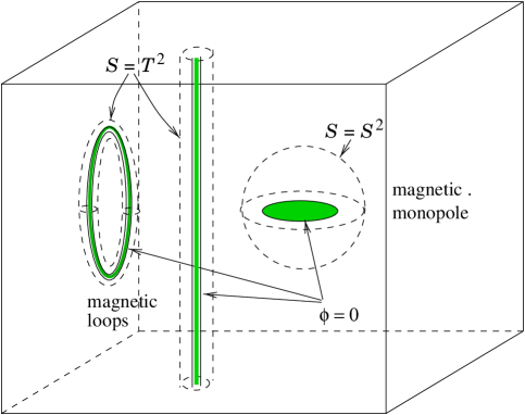
Figure 3: The magnetic flux through closed surfaces is equals the winding of the normalised Higgs field ${\cal S}\to S^{2}$

$$n({\cal S})={1\over 16\pi i}\oint_{{\cal S}}\mbox{Tr}\left(\hat{\phi}\,{\mbox{d}}\hat{\phi}\wedge{\mbox{d}}\hat{\phi}\right).$$

The magnetic flux through ${\cal S}$ is defined by

$$\Phi({\cal S})=\oint_{{\cal S}}F_{\rm mag}.$$

In Appendix B we show that

$$\begin{array}[]{rcl}\displaystyle\mbox{Tr}\left(\hat{\phi}\,{\mbox{d}}\hat{\phi}\wedge{\mbox{d}}\hat{\phi}\right)=8iF_{\rm mag}\end{array}$$ (5.6)

and hence

$$\begin{array}[]{rcl}\displaystyle n({\cal S})=\frac{1}{2\pi}\Phi({\cal S}).\end{array}$$ (5.8)

That is the magnetic charge of the defect is proportional to the winding number of the Higgs field $\hat{\phi}:{\cal S}\rightarrow S^{2}$. Hence it is quantised. Actually, if ${\cal S}$ is a two-sphere surrounding a magnetic monopole then $A_{\rm mag}|_{\cal S}$ may be viewed as the Abelian gauge potential of the Schwinger model on $S^{2}$ [21], if ${\cal S}$ is a two-torus as the gauge potential of the Schwinger model on $T^{2}$ [22]. The quantised flux $\Phi$ is just the quantised instanton number of the Schwinger model on $S^{2}$ or $T^{2}$.

We now look at the relation between the winding numbers of the defects (and hence the magnetic charges) and the instanton number $q$. We again assume that we only have no walls. In this case the Higgs field, $\phi(\vec{x})$, can be assumed to be smooth throughout $T^{3}$ except at the the ${\cal P}=-1\!\mbox{l}$ defects, where it is ill defined. At the ${\cal P}=1\!\mbox{l}$ defects the Higgs field is zero. In Appendix B we derive the following relation between $\hbox{Tr}\left(({\cal P}^{-1}d{\cal P})^{3}\right)$ and the Higgs field $\phi$

$$\begin{array}[]{rcl}\displaystyle 2i\hbox{Tr}({\cal P}^{-1}d{\cal P})^{3}=3{\mbox{d}}\Big{[}\big{(}|\phi|-\hbox{${1\over 2}$}\sin(2|\phi|)\big{)}\mbox{Tr}\big{(}\hat{\phi}\,{\mbox{d}}\hat{\phi}\wedge d\hat{\phi}\big{)}\Big{]},\end{array}$$ (5.10)

$\hat{\phi}$ being the normalised Higgs field. Note that the right hand side of (5.10) is ill-defined both where ${\cal P}=1\!\mbox{l}$ and ${\cal P}=-1\!\mbox{l}$. Using the instanton number formula (LABEL:polloopindex) and (5.10) we can write the topological charge as a functional of the Higgs field

$$\begin{array}[]{rcl}\displaystyle q=\frac{1}{16\pi^{2}i}\int_{{\cal D}^{c}}{\mbox{d}}\Big{[}\big{(}|\phi|-\hbox{${1\over 2}$}\sin(2|\phi|)\big{)}\mbox{Tr}\big{(}\hat{\phi}\,{\mbox{d}}\hat{\phi}\wedge\hat{d}\phi\big{)}\Big{]}.\end{array}$$ (5.12)

Before we can apply Stokes theorem we must exclude closed sets (with infinitesimal volume in ${\cal D}^{c}$) surrounding both ${\cal P}=1\!\mbox{l}$ and ${\cal P}=-1\!\mbox{l}$ defects. Thus we have

$$\begin{array}[]{rcl}\displaystyle q=\frac{1}{16\pi^{2}i}\sum_{i}\oint_{{\cal S}_{i}}\big{(}|\phi|-\hbox{${1\over 2}$}\sin(2|\phi|\big{)}\mbox{Tr}\big{(}\hat{\phi}\,{\mbox{d}}\hat{\phi}\wedge\hat{\phi}\big{)}.\end{array}$$ (5.14)

where the ${\cal S}_{i}$ are surfaces surrounding the defects. Note that the factor $|\phi|-\hbox{${1\over 2}$}\sin(2|\phi|)$ behaves very differently in the neighbourhoods of the two kinds of defects. Near a defect with ${\cal P}=1\!\mbox{l}$ the Higgs field tends to zero and the factor vanishes as $\sim|\phi|^{3}$. Since $\oint_{{\cal S}}\mbox{Tr}(\hat{\phi}\,d\hat{\phi}\wedge\hat{\phi})$ stays finite if we approach such a defect the integrals in (5.14) vanish when the surrounding surfaces approach defects with ${\cal P}=1\!\mbox{l}$. On the other hand, in the neighbourhood of the ${\cal P}=-1\!\mbox{l}$ defects we have $|\phi|\sim\pi$ so that $\big{(}|\phi|-\sin(2|\phi|)/2\big{)}\sim\pi$, from which follows that

$$\begin{array}[]{rcl}\displaystyle q=\frac{1}{16\pi i}\sum_{\hbox{\footnotesize{${\cal P}=-1\!\mbox{l}$ defects}}}\oint_{{\cal S}_{i}}\mbox{Tr}\big{(}\hat{\phi}\,{\mbox{d}}\hat{\phi}\wedge{\mbox{d}}\hat{\phi}\big{)}.\end{array}$$ (5.16)

At this point it is convenient to define an alternative Higgs field $\phi_{alt}(\vec{x})$ through

$${\cal P}(\vec{x})=-\exp\left[i\phi_{alt}(\vec{x})\right],$$

where now $\phi_{alt}(\vec{x})$ is smooth and zero at ${{\cal P}=-1\!\mbox{l}}$, but ill defined at the ${\cal P}=1\!\mbox{l}$ defects. In the absence of walls we have that both $|\phi(\vec{x})|$ and $|\phi_{alt}(\vec{x})|$ are in the interval $[0,\pi)$. In ${\cal D}^{c}$ one has the following relations between the two Higgs fields

$$\begin{array}[]{rcl}\displaystyle|\phi|=\pi-|\phi_{alt}|,\quad\hat{\phi}_{alt}=-\hat{\phi}.\end{array}$$ (5.18)

Using this we see that the topological charge is proportional to the sum of winding numbers of $\phi_{alt}$ around the ${\cal P}=-1\!\mbox{l}$ defects

$$\begin{array}[]{rcl}\displaystyle q=-\frac{1}{16\pi i}\sum_{\hbox{\footnotesize{${\cal P}=-1\!\mbox{l}$ defects}}}\oint_{{\cal S}_{i}}\mbox{Tr}\big{(}\hat{\phi}_{alt}\,{\mbox{d}}\hat{\phi}_{alt}\wedge{\mbox{d}}\hat{\phi}_{alt}\big{)}.\end{array}$$ (5.20)

The orientation of integration in this equation is such that the normal vector on the surface ${{\cal S}_{i}}$ points inside the surface (onto the monopole). But in equation (LABEL:magnwind3) the orientation of integration is opposite. Therefore we conclude

$$\begin{array}[]{rcl}\displaystyle q=\sum_{\hbox{\footnotesize{${\cal P}=-1\!\mbox{l}$ defects}}}n_{alt}({\cal S}_{i}).\end{array}$$ (5.22)

Hence the instanton number is the sum over the winding numbers of the Higgs field $\phi_{alt}$ at ${\cal P}=-1\!\mbox{l}$ defects. Taking into account equation (5.18) we obtain

$$\begin{array}[]{rcl}\displaystyle\mbox{Tr}\left(\hat{\phi}_{alt}\,{\mbox{d}}\hat{\phi}_{alt}\wedge{\mbox{d}}\hat{\phi}_{alt}\right)=-8iF_{\rm mag}.\end{array}$$ (5.24)

Thus a ${\cal P}=-1\!\mbox{l}$ defect with winding number $n_{alt}$ has magnetic charge $-n_{alt}$. Similar considerations yield that the instanton number $q$ is given by the sum over winding numbers of the Higgs field $\phi$ at ${\cal P}=1\!\mbox{l}$ defects, or equivalently, by the sum of all monopole charges at ${\cal P}=1\!\mbox{l}$ defects. The relation between the instanton number and the magnetic charges of pointlike monopoles on $\mbox{l}\!\mbox{R}^{4}$ has already been obtained by Reinhardt [11].

For a non-zero flux the magnetic potential $A_{\rm mag}$ must necessarily be singular somewhere on ${\cal S}$, else the flux $\oint dA_{\rm mag}$ would vanish. As is well-known from the Dirac monopole, we may assume that $A_{\rm mag}$ is regular on ${\cal S}$ with one point removed. Since this holds true for any ${\cal S}\subset{\cal D}^{c}$ surrounding a charged defect we must attach a string to each such defect on which $A_{\rm mag}$ is singular. By definition, wherever the magnetic potential is singular the diagonalisation matrix $W(\vec{x})$ is singular.

Let us now consider a $S^{2}\subset{\cal D}^{c}$ surrounding a monopole-antimonopole pair. On such a sphere the Higgs field has no winding and can smoothly be diagonalised. This means that the strings on which $W(\vec{x})$ (and $A_{\rm mag}$) is singular start and end at defects with opposite magnetic charge. Outside of these strings it is possible to choose $W$ smooth. A possible distribution of monopoles connected by strings is shown in fig.4. The string positions are gauge dependent. But they must start and end at (anti)monopoles whose positions are gauge invariant.

Figure 4: The smooth diagonalisation of ${\cal P}(\vec{x})$ fails on strings connecting monopoles and anti-monopoles of opposite charges. Shown is a string-network in the sector with instanton number $q=4$

There is some freedom regarding which defects are connected to each other with Dirac strings. Suppose we have a Dirac string emanating from a ${\cal P}=1\!\mbox{l}$ defect. Then this string may be connected to either a ${\cal P}=1\!\mbox{l}$ or ${\cal P}=-1\!\mbox{l}$ defect with the opposite charge. We have shown that the instanton number, $q$, is proportional to the total magnetic charge at ${\cal P}=1\!\mbox{l}$ defects. We can restate this result in terms of the Dirac strings as follows; $q$ is proportional to the number of Dirac strings joining ${\cal P}=1\!\mbox{l}$ and ${\cal P}=-1\!\mbox{l}$ defects. In fact, it is possible to rewrite the instanton number formula (LABEL:polloopindex) so that the contribution of the strings is transparent without introducing Higgs fields. This calculation is given in Appendix B.

To gain further insight we investigate ${\cal P}$ in the vicinity of a point defect (see also [18]). For that we follow the eigenvalues along a closed path from $p$ to $p$ (see fig.2a) passing through a monopole. We may slightly deform this path so that it misses the monopole. On the deformed path the eigenvalues of ${\cal P}$ are nowhere degenerate and thus $H$ in (LABEL:diagonalization) must be periodic (see above). Returning to the undeformed path through the monopole we conclude, that at the monopole, where both eigenvalues are $1$, the two eigenvalues are reflected at $\lambda=1$ as shown in fig.2a. The spectral flow is continuous but not differentiable. Since ${\cal P}(\vec{x})$ is smooth, the diagonalising $W(\vec{x})$ in (LABEL:diagonalization) must be singular to compensate for the non-smoothness of $D(\vec{x})$. As in the case without defects, $W(\vec{x})$ is not necessarily periodic and obeys (LABEL:hilfs1).

To summarise, in the presence of monopole and loop defects we can still perform the gauge transformation (LABEL:gauge-trf-1). But it is necessarily singular on strings connecting the defects. The gauge transformed $A_{0}(\vec{x})$ is periodic, but singular on these strings. After gauge fixing the transition functions can be chosen as in (LABEL:simpletrans). The instanton number is related to the magnetic charges of the defects in a very simple way.

In cases where domain walls extend over the whole torus the situation is analogous to the one in $2$-dimensional gauge theories. We cannot avoid defects when going from one “face” of the torus to the opposite one. There is no obstruction for the eigenvalues to vary smoothly along a path crossing the wall. Neither $H$ nor $W$ are singular at the wall (see fig.2). But the eigenvalues of $H$ may wind or interchange if we move from $\vec{x}$ to $\vec{x}+b_{i}$ and thus $D(\vec{x})$ may be periodic only up to a permutation of its entries, i.e.

$$H(\vec{x}+b_{i})={\cal W}_{i}H(\vec{x}){\cal W}_{i}^{-1}+\hat{H}_{i},$$

where the ${\cal W}_{i}$ are Weyl-reflections and the $\hat{H}_{i}\in{\cal L}$, with ${\cal L}$ being the discrete lattice defined in (LABEL:discrete). Now we can only prove, that the gauge transformed transition functions have the form

$$U_{0}=1\!\mbox{l},\quad U_{i}=e^{-2\pi i\xi_{0}\hat{H}_{i}}R_{i}(\vec{x}){\cal W}_{i},$$

where again the $R_{i}$ are in the Abelian subgroup and fulfil the cocycle condition (LABEL:cocycle). This time dependence in the transition functions is reminiscent of the $T^{2}$ analysis [8]. The gauge fixed $A_{0}$ has the form

$$A_{0}(\vec{x})=a_{0}(\vec{x})+{2\pi\over L_{0}}\sum_{i=1}^{3}\hat{H}_{i}\xi_{i},\quad\hbox{{where}}\quad a_{0}(\vec{x}+b_{i})={\cal W}_{i}a_{0}(\vec{x}){\cal W}_{i}^{-1}.$$

As in the case without defects there are residual gauge transformations (see Appendix C).

6 Conclusions and Outlook

In this paper we have considered the gauge-fixing of Yang-Mills theory on the four torus for arbitrary instanton sectors. Of course the choice of gauge fixing does not affect physics, but an appropriate gauge-fixing may considerably simplify the mathematical problem of computing or approximating functional integrals. Motivated by their success in two dimensions we adopted an extended Abelian projection on the four torus. Here we require $A_{0}$ to be Abelian, time independent and the spatial components $A_{i}$ of the gauge potential to be periodic in time.

One difference with the $T^{2}$ problem is that we have the added complication of instanton sectors. In two dimensions one may assume that before gauge fixing the gauge potential $A_{\mu}$ is completely periodic, ie. the transition functions are trivial $U_{\mu}=1\!\mbox{l}$. In four dimensions, we may only assume this if we are in the zero instanton sector (ie. the topological charge $q$ is zero). We have argued that for $q\neq 0$ it is convenient to work with a new set of non-Abelian transition functions. With these transition functions the path ordered exponential, ${\cal P}(\vec{x})$, which is central to the gauge fixing is completely periodic, even though of course the gauge field itself is non-periodic. Moreover, these transition functions include the odd instanton sectors of $SU(2)$. To our knowledge, smooth untwisted transition functions for this case have not been given before.

The most significant break with the two dimensional treatment is the presence of unavoidable singularities in the final gauge fixed potential [7]. These singularities are due to ambiguities in the diagonalisation of ${\cal P}(\vec{x})$ where the eigenvalues of ${\cal P}(\vec{x})$ are degenerate (for $SU(2)$ this degeneracy occurs where ${\cal P}(\vec{x})=\pm 1\!\mbox{l}$). There is a close analogy between these defects (ie. points, loops or surfaces where ${\cal P}(\vec{x})$ is degenerate) and magnetic charges in Yang-Mills-Higgs theories [23]. We have presented a detailed analysis of the special case where one only has point and loop defects, which can be interpreted as magnetic monopoles and magnetised loops. The gauge fixed potential is smooth everywhere except for “Dirac strings” joining monopole (loop) pairs. The instanton number, $q$ is simply the number of magnetic charges at the ${\cal P}=1\!\mbox{l}$ defects.

¿From one viewpoint the existence of these magnetic defects imply that our attempt to generalise the two dimensional fixing has failed. We take the opposite view. It is a long standing conjecture that confinement of color is produced by dual superconductivity (of type II) of the QCD vacuum [24]. Indeed, lattice calculations [25] indicate that magnetic monopoles (or loops?) are the dominant infrared degrees of freedom, at least in the maximal Abelian gauge and the Polyakov gauge.

There is a long way from the picture of condensed magnetic monopoles to real $QCD$. At present there is no analytic proof of the existence of the condensate of monopoles. However, in those theories where we understand confinement, the latter is due to the condensation of monopoles; these examples are compact $QED$ [26] and supersymmetric Yang-Mills theories [27]. The balancing of the energy and the entropy of monopoles (and/or loops) may explain the occurrence of the deconfinement transition in $QCD$. At low temperatures we expect a condensation of monopoles with ${\cal P}=1\!\mbox{l}$ and of monopoles with ${\cal P}=-1\!\mbox{l}$. In the broken high temperature phase, where $\langle\mbox{Tr}{\cal P}\rangle\sim\pm 2$, we do not expect long monopole loops but rather a dipole gas of monopole-antimonopole pairs, both with ${\cal P}=1\!\mbox{l}$ (or both with ${\cal P}=-1\!\mbox{l}$).

Of course the treatment given here has been purely classical. The next step would be to study the path integral within this gauge fixing. At this point one would need a suitable approximation [28]. With a view to investigating the confinement of static quarks it would be interesting to consider whether in any regime the monopoles and Dirac strings play a dominant role in the path integral.

Appendices

Appendix A Theta Functions

Our conventions with respect to theta functions are the same as ref. [29]. We work with the Jacobi theta function with characteristics

$$\begin{array}[]{rcl}\displaystyle\theta\left[\begin{array}[]{c}\displaystyle a\\ b\end{array}\right](z,i\tau)=\sum_{n\in Z}e^{-\pi\tau(n+a)^{2}+2\pi i(n+a)(z+b)}.\end{array}$$ (A.4)

This function has the following periodicity properties

$$\begin{array}[]{rcl}\displaystyle\theta\left[\begin{array}[]{c}\displaystyle a+m\\ b+n\end{array}\right](z,i\tau)=e^{2\pi ina}\theta\left[\begin{array}[]{c}\displaystyle a\\ b\end{array}\right](z,i\tau),\quad m,n\in Z\end{array}$$ (A.10)

and has zeros where $z=(a+n+\frac{1}{2})\tau+(b+m+\frac{1}{2}),\ n,m\in Z$.

Appendix B Technical Results

In this appendix we derive some of the technical results quoted in chapter 5.

B.1 Magnetic Charges and Higgs winding numbers

To relate this winding number to the magnetic flux we parameterise the normalised Higgs field as

$$\hat{\phi}=\big{(}\sin\theta\cos\varphi,\sin\theta\sin\varphi,\cos\theta\big{)},\qquad\phi=|\phi|\hat{\phi}_{i}\sigma_{i},$$

where the angles $\theta,\varphi$ are functions on ${\cal S}$. The corresponding ${\cal P}=\exp(i\phi)$ is diagonalised by [30]

$$W=\exp(-i{\varphi\over 2}\sigma_{3})\exp(-i{\theta\over 2}\sigma_{2})\exp(i\lambda\sigma_{3})\quad\hbox{{and}}\quad D=\exp(i|\phi|\sigma_{3}).$$

The magnetic potential (LABEL:magnpot) is $A_{\rm mag}=d\lambda-{1\over 2}\cos\theta d\varphi$, and the corresponding field strength is

$$F_{\rm mag}={1\over 2}\sin\theta{\mbox{d}}\theta\wedge{\mbox{d}}\varphi.$$

On the other hand, taking the Higgs field (LABEL:higgs) we get

$$\begin{array}[]{rcl}\displaystyle\mbox{Tr}\left(\hat{\phi}{\mbox{d}}\hat{\phi}\wedge{\mbox{d}}\hat{\phi}\right)=4i\sin\theta{\mbox{d}}\theta\wedge{\mbox{d}}\varphi=8iF_{\rm mag}.\end{array}$$ (B.3)

Comparing with equations (LABEL:magnwind3) and (LABEL:magnwind1) one readily obtains

$$n({\cal S})={1\over 2\pi}\oint_{{\cal S}}\sin\theta\;d\theta\wedge d\varphi={1\over 2\pi}\Phi({\cal S}).$$

B.2 Derivation of equation (5.10)

Now we will relate $\mbox{Tr}\left(\left({\cal P}^{-1}{\mbox{d}}{\cal P}\right)^{3}\right)$ to the Higgs field $\phi=\phi_{\alpha}\sigma^{\alpha}$. With the notation $|\phi|=\sqrt{\mbox{Tr}\phi^{2}/2}$ and $\hat{\phi}:=\phi/|\phi|$ we have ${\cal P}=\exp\left(i\phi\right)=\cos(|\phi|)+i\sin(|\phi|)\hat{\phi}$ and it follows that

$$\begin{array}[]{rcl}\displaystyle({\cal P}^{-1}{\mbox{d}}{\cal P})^{3}&=&-\sin^{4}|\phi|\hat{\phi}{\mbox{d}}\hat{\phi}\wedge{\mbox{d}}\hat{\phi}\wedge{\mbox{d}}\hat{\phi}-i\sin^{3}|\phi|\cos|\phi|{\mbox{d}}\hat{\phi}\wedge{\mbox{d}}\hat{\phi}\wedge{\mbox{d}}\hat{\phi}\\ &&\displaystyle-3i\sin^{2}|\phi|\hat{\phi}{\mbox{d}}\hat{\phi}\wedge{\mbox{d}}\hat{\phi}\wedge{\mbox{d}}|\phi|.\end{array}$$ (B.7)

Under the trace the first two terms on the right hand side of (B.7) drop out. Hence we have

$$\mbox{Tr}\left(({\cal P}^{-1}{\mbox{d}}{\cal P})^{3}\right) = -3i\sin^{2}|\phi|{\mbox{d}}|\phi|\wedge\mbox{Tr}\left(\hat{\phi}{\mbox{d}}\hat{\phi}\wedge{\mbox{d}}\hat{\phi}\right)$$ (B.8)

$$= {\mbox{d}}\left\{\frac{3}{2i}\left(|\phi|-\frac{\sin(2|\phi|)}{2}\right)\mbox{Tr}\left(\hat{\phi}{\mbox{d}}\hat{\phi}\wedge{\mbox{d}}\hat{\phi}\right)\right\}.$$

B.3 Instanton number and Dirac Strings

We showed in the paper that in the presence of magnetic monopoles the diagonalization is not smoothly possible. The matrix $W$ becomes singular on Dirac strings connecting monopoles with opposite magnetic charges. We shall argue that the strings on which $W$ is singular contribute to the instanton number $q$. Setting ${\cal P}=WDW^{-1}$ one first observes for arbitrary gauge groups that

$$\mbox{Tr}\left(({\cal P}^{-1}{\mbox{d}}{\cal P})^{3}\right)={\mbox{d}}{\cal A},$$

where the $2$-form ${\cal A}$ is

$${\cal A}=-6\mbox{Tr}\left(W^{-1}{\mbox{d}}W\wedge D^{-1}{\mbox{d}}D\right)+3\mbox{Tr}\left(W^{-1}{\mbox{d}}WD^{-1}\wedge W^{-1}{\mbox{d}}WD\right).$$

Thus we can convert the integral in (LABEL:polloopindex) into a surface integral over the “boundary” of the torus and over infinitesimal cylinders around the strings (see fig.4):

$$q=\frac{1}{24\pi^{2}}\int\mbox{Tr}\left(({\cal P}^{-1}{\mbox{d}}{\cal P})^{3}\right)=q_{{\rm s}}+q_{{\rm b}},$$

where the individual contributions from the strings and boundary of the torus read

$$q_{\rm s}=\frac{1}{24\pi^{2}}\sum_{\rm strings}\;\int\limits_{\rm cyl.}{\cal A}\;\quad\hbox{{and}}\quad\;q_{\rm b}=\frac{1}{24\pi^{2}}\sum_{i=1}^{3}\Big{(}\int\limits_{x_{i}=0}\big{(}{\cal A}(x+b_{i})-{\cal A}(x)\big{)}\Big{)}.$$

If only monopoles are present, then $H(\vec{x})$ is periodic and $W(\vec{x}+b_{i})=W(\vec{x})R_{i}(\vec{x})$, where the $R_{i}$ are abelian and satisfy the cocycle conditions (4.10). After some algebra we obtain

$${\cal A}(x+b_{i})-{\cal A}(x)=-6\mbox{Tr}\big{(}R_{i}(x)^{-1}{\mbox{d}}R_{i}(x)\wedge D(x)^{-1}{\mbox{d}}D(x)\big{)}.$$

We parametrize the diagonal matrix as

$$\begin{array}[]{rcl}\displaystyle D=e^{i\alpha\sigma_{3}}\quad\hbox{{so that}}\quad D^{-1}{\mbox{d}}D=i{\mbox{d}}\alpha\sigma_{3}\end{array}$$ (B.10)

and arrive at

$$q_{\rm b} = {1\over 4i\pi^{2}}\sum_{i=1}^{3}\int_{x_{i}=0}{\mbox{d}}\Big{[}\alpha\mbox{Tr}(R_{i}^{-1}{\mbox{d}}R_{i}\sigma_{3})\Big{]}$$

$$= \frac{1}{4i\pi^{2}}\sum_{i,j}\int_{x_{i}=x_{j}=0}\varepsilon_{ijk}\alpha\mbox{Tr}\left(\left(R_{i}(x+b_{j})^{-1}\partial_{k}R_{i}(x+b_{j})-R_{i}(x)^{-1}\partial_{k}R_{i}(x)\right)i\sigma_{3}\right)dx^{k}\quad.$$

Differentiating equation (4.10) one sees that the trace term is symmetric in $i$ and $j$. Therefore we conclude $q_{\rm b}=0$ in accordance with the fact that the spatial transition functions are simply given by the functions $R_{i}$, see equation (LABEL:transition-fct-2D).

The strings do contribute to the instanton number. We consider a Dirac string connecting monopoles. We argue that this string contributes to the instanton number the sum of monopole charges of ${\cal P}=1\!\mbox{l}$ monopoles attached to the string. Using the parametrisation (B.10) we can write

$$\begin{array}[]{rcl}\displaystyle{\cal A}&=&-12{\mbox{d}}\alpha\wedge A_{\rm mag}+12\sin\alpha\cos\alpha F_{\rm mag}\\ &=&-12{\mbox{d}}(\alpha+\sin\alpha\cos\alpha)\wedge A_{\rm mag}+12{\mbox{d}}(\sin\alpha\cos\alpha A_{\rm mag}).\end{array}$$ (B.14)

Integrating over a closed surface ${\cal S}$ surrounding the string the contribution from the second term vanishes. Now we choose a ${\cal P}=1\!\mbox{l}$ monopole and the Dirac string emanating from it. We introduce coordinates $(z,\varphi)$ on ${\cal S}$ such that $\alpha$ is independent of $\varphi$. The contribution of the string to the instanton number reads

$$\begin{array}[]{rcl}\displaystyle\frac{1}{24\pi^{2}}\oint_{{\cal S}}{\cal A}=-\frac{1}{2\pi^{2}}\int{\mbox{d}}z\frac{\partial}{\partial z}\left(\alpha+\sin\alpha\cos\alpha\right)\int{\mbox{d}}\varphi A_{{\rm mag}\,\varphi}.\end{array}$$ (B.16)

The integral $\int{\mbox{d}}\varphi A_{{\rm mag}\,\varphi}$ is up to the sign given by the magnetic flux through the Dirac string, ie. it is $-2\pi$ times the magnetic charge of the ${\cal P}=1\!\mbox{l}$ monopole. Therefore the contribution of the string to the instanton number is given by $(1/\pi)\Delta(\alpha+\sin\alpha\cos\alpha)$. Hence, if the string ends at a ${\cal P}=-1\!\mbox{l}$ monopole then it contributes $1\,\,(\Delta\alpha=\pi)$ and, if it ends at a ${\cal P}=1\!\mbox{l}$ monopole $(\Delta\alpha=0)$, it will not contribute. The generalisation to arbitrary strings is straightforward.

Appendix C Residual Gauge Fixing

After the gauge fixing procedure described in sections 4 and 5, $A_{0}$ is independent of time and restricted to the Cartan subalgebra. Furthermore, the transition functions become abelian (upto an element of the Weyl group if one has wall defects). However, the gauge is not fixed completely, since one must fix the residual gauge freedom related to gauge transformations which preserve the properties of $A_{0}$ mentioned above. If we have no walls we may assume that the transition functions have the standard form (LABEL:simpletrans). Thus we only consider residual gauge transformations which do not change the transition functions. One may regard this fixing of the transition functions as the first part of our residual gauge fixing. Let us first consider the case considered in chapter 4, where one has no defects.

C.1 No defects

Here we assume that the defect manifold ${\cal D}$ is empty, in which case ${\cal P}(\vec{x})$ is smoothly diagonalisable. We may also assume that $H(\vec{x})$ is smoothly restricted to the first Weyl chamber. After the first part of the gauge fixing given in section four the transition functions are abelian. The residual gauge transformations are

$$V(x)=\exp\left\{2\pi i\left(H_{per}(\vec{x})+H_{i}\frac{x_{i}}{L_{i}}\right)\right\},$$ (C.1)

where all $H$’s are in the Cartan subalgebra, $H_{per}$ is periodic in all spatial directions, and $H_{i}\in{\cal L}$. Clearly these residual gauge transformations have no effect on $A_{0}$. Accordingly, to fix the gauge we must impose constraints on the spatial components of the gauge field. Of course, $A_{i}(x)$ depends on time, whereas the residual gauge transformations under consideration are time-independent. Thus we could impose constraints on $A_{i}$ for some fixed time, say $x_{0}=0$. Alternatively, if we wish to treat all times on an equal footing we can consider the time-averaged object

$$\begin{array}[]{rcl}\displaystyle\tilde{A}_{i}(\vec{x})=\frac{1}{L_{0}}\int^{L_{0}}_{0}dx_{0}A_{i}(x_{0},\vec{x}).\end{array}$$ (C.3)

Using the result that the transition functions are Abelian after gauge-fixing, the Cartan part of $\tilde{A}_{i}(\vec{x})$ (or $A_{i}(x_{0}=0,\vec{x})$) may be decomposed into a periodic piece $\tilde{A}_{i}^{c,per}$ and a contribution $\tilde{A}_{i}^{c,lin}$, which is linear in the spatial coordinates. If we impose

$$\begin{array}[]{rcl}\displaystyle{1\over{L_{1}L_{2}L_{3}}}\int_{T^{3}}\tilde{A}_{i}^{c,per}d^{3}x\in\;{2\pi\over L_{i}}\cdot{\cal H}/{{\cal L}},\quad i=1,2,3,\end{array}$$ (C.5)

we fix the gauge freedom with respect to the $H_{i}$. Here ${\cal H}/{\cal L}$ is the torus obtained by dividing the Cartan subalgebra ${\cal H}$ by the lattice ${\cal L}$.

If we demand the following relations, we can fix the residual gauge freedom concerning $H_{per}$ upto an Abelian global gauge transformation

$$\begin{array}[]{rcl}\displaystyle\tilde{A}^{c,per}_{1}=h_{1}(x_{2},x_{3}),\quad\int\limits_{0}^{L_{1}}\tilde{A}^{c,per}_{2}dx_{1}=h_{2}(x_{3}),\quad\int\limits_{0}^{L_{1}}\int\limits_{0}^{L_{2}}\tilde{A}^{c,per}_{3}dx_{1}dx_{2}=h_{3},\end{array}$$ (C.7)

where the functions $h_{i}$ are Cartan subalgebra valued functions of the relevant spatial coordinates. An alternative to (C.7) which is symmetric in the spatial variables is simply the Coulomb type condition

$$\begin{array}[]{rcl}\displaystyle\nabla\cdot\tilde{\bf A}^{c,per}(\vec{x})=0.\end{array}$$ (C.9)

C.2 Defects without walls

We now assume that the defect manifold, ${\cal D}$, is non-empty. Thus our gauge fixed potential is not well defined for $\vec{x}\in{\cal D}$ and on the Dirac strings joining the defects. While ${\cal D}$ is gauge invariant, the paths taken by the Dirac strings are not. However, one can only change the path of the Dirac strings with a singular gauge transformation. The residual gauge transformations considered in the previous subsection were (implicitly) assumed to be smooth. Thus it is convenient to separate the residual gauge fixing into two parts. Firstly, one fixes the location of the Dirac strings (which can be viewed as a singular residual gauge fixing). For example consider the case where one only has point-like monopole defects. Here one can take the Dirac strings to be straight lines all meeting together in the centre of $T^{3}$. Then one repeats the residual gauge fixing of section C.1, except that now one must exclude a closed set, $\cal G$, containing both the defect manifold ${\cal D}$ and the (by now fixed) Dirac strings from the relevant integrals in (C.7).

C.3 Walls

If we allow for wall defects then we actually have a wider class of residual gauge transformations

$$V(x)={\cal W}\cdot\exp\left\{2\pi i\left(H_{per}(\vec{x})+H_{i}\frac{x_{i}}{L_{i}}+H_{0}\frac{x_{0}}{L_{0}}\right)\right\},$$ (C.10)

where $H_{0}\in{\cal L}$, and ${\cal W}$ is an element of the Weyl group which commutes with all the transition functions.The reason for this extra freedom is that in the cases considered in the previous subsections we could assume that $H(\vec{x})$ is restricted to the first Weyl chamber, and we only considered residual gauge transformations which respected this constraint.

References

- [1] T. Suzuki, Nucl. Phys. (Proc. Suppl.) B30, 176, 1993 and references therein.
- [2] K.G. Wilson, Phys. Rev. D10, 2445, 1974.
- [3] A.M. Polyakov, Phys. Lett. 72B, 477, 1978; L. Susskind, Phys. Rev. D20, 2610, 1979.
- [4] S.J. Gates, M.T. Grisaru, M. Rocek and W. Siegel, Superspace or One Thousand and One Lessons in Supersymmetry , Benjamin-Cummings 1983; P. West, Phys. Lett. B258, 375, 1991; I. Jack and D.R.T. Jones, Phys. Lett. B258, 382, 1991.
- [5] L.P. Kadanoff, Physica 2, 263, 1966; K.G. Wilson, Phys. Rev. B4, 3174, 1971; K.G. Wilson and I.G. Kogut, Phys. Rep. 12, 75, 1974.
- [6] D.J. Gross, R.D. Pisarski and L.G. Yaffe, Rev. Mod. Phys. 53, 43, 1981; J.I. Kapusta, Finite-temperature field theory, Cambridge University Press, 1989.
- [7] G. ’t Hooft, Nucl. Phys. B190, 455, 1981.
- [8] U. G. Mitreuter, J. M. Pawlowski and A. Wipf, Nucl. Phys. B, in press, hep-th/9611105.
- [9] G. ’t Hooft, Comm. Math. Phys. 81, 267, 1981.
- [10] P.A.M. Dirac, Proc. Roy. Soc. A133, 60, 1931.
- [11] H. Reinhardt, Nucl. Phys. B 503, 505, 1997.
- [12] P. van Baal, Comm. Math. Phys. 85, 529, 1982.
- [13] M.F. Atiyah, N.J. Hitchin, V.G. Drinfeld and Yu.I. Manin, Phys. Lett. A65, 185, 1978; N.H. Christ, E.J. Weinberg and N.K. Stanton, Phys. Rev. D18, 2013, 1978; E. Corrigan, D.B. Fairlie, P. Goddard and S. Templeton, Nucl. Phys. B140, 31, 1978.
- [14] W. Nahm, Phys. Lett. B 90, 413, 1980.
- [15] P. van Baal, Nucl. Phys. Proc. Suppl. 49, 238, 1996.
- [16] M. Garcia Perez, A. Gonzalez-Arroyo and B. Sorenberg, Phys. Lett. B235, 117, 1990
- [17] C. Taubes, J. Diff. Geom. 19, 517, 1984.
- [18] H. W. Grießhammer, Magnetic Defects Signal Failure of Abelian Projection Gauges in QCD, hep-ph/9709462.
- [19] A.S. Kronfeld, G. Schierholz and U.J. Wiese, Nucl. Phys. B293, 461, 1987.
- [20] S.P. Novikov and A.T. Fomenko, Elements of Differential Geometry for Physicists, Soviet Physics - Uspekhi 25, 1982.
- [21] C. Jayewardena, Helv. Phys. Acta 61, 636, 1988.
- [22] I. Sachs and A. Wipf, Helv. Phys. Acta 65, 653, 1992; Ann. Phys. (NY) 249, 380, 1996.
- [23] G. ’t Hooft, Nucl. Phys. B79 (1974) 194; A.M. Polyakov, JETP lett. 20 (1974) 194.
- [24] G. ’t Hooft, in High Energy Physics, EPS International Conference, Palermo 1975, ed. A. Zichini; S. Mandelstam, Phys. Rep. 23C, 245, 1976; G. Parisi, Phys. Rev. D11, 971, 1975.
- [25] See M.N. Chernodub and M.I. Polikarpov, hep-th/9710205 and references therein; L. Del Debbio, A. Di Giacomo, G. Pafitti and P. Pier, Phys. Lett. B355, 255, 1995; L. Del Debbio, M. Faber, J. Greensite and S. Olejnek, hep-lat/9610005.
- [26] A.M. Polyakov, Phys.Lett. 59B, 82, 1975; T. Banks, R. Myerson and J. Kogut, Nucl. Phys. B129, 493, 1977.
- [27] N. Seiberg and E. Witten, Nucl. Phys. B341, 484, 1994.
- [28] F. Lenz and M. Thies, Polyakov Loops Dynamics in the Center Symmetric Case, preprint FAU-TP3-98, hep-th/9802066.
- [29] D. Mumford, Tata Lectures about Theta I, Boston, Birkhäuser, 1983.
- [30] J. Kijowski and G. Rudolph, Nucl. Phys. B325 211, 1989.