hep-th/9802085

KEK-TH-559

TIT/HEP-382

Space-Time Structures from IIB Matrix Model

Hajime Aoki¹⁾, Satoshi Iso¹⁾, Hikaru Kawai¹⁾,

Yoshihisa Kitazawa²⁾and Tsukasa Tada¹⁾

¹⁾ High Energy Accelerator Research Organization (KEK),
Tsukuba, Ibaraki 305, Japan

²⁾ Department of Physics, Tokyo Institute of Technology,

Oh-okayama, Meguro-ku, Tokyo 152, Japan

We derive a long distance effective action for space-time coordinates from a IIB matrix model. It provides us an effective tool to study the structures of space-time. We prove the finiteness of the theory for finite $N$ to all orders of the perturbation theory. Space-time is shown to be inseparable and its dimensionality is dynamically determined. The IIB matrix model contains a mechanism to ensure the vanishing cosmological constant which does not rely on the manifest supersymmetry. We discuss possible mechanisms to obtain realistic dimensionality and gauge groups from the IIB matrix model.

1 Introduction

A large $N$ reduced model has been proposed as a nonperturbative formulation of type IIB superstring theory[1][2]. It is defined by the following action:

$$S=-{1\over g^{2}}Tr({1\over 4}[A_{\mu},A_{\nu}][A^{\mu},A^{\nu}]+{1\over 2}\bar{\psi}\Gamma^{\mu}[A_{\mu},\psi]),$$ (1.1)

here $\psi$ is a ten dimensional Majorana-Weyl spinor field, and $A_{\mu}$ and $\psi$ are $N\times N$ Hermitian matrices. It is formulated in a manifestly covariant way which we believe is a definite advantage over the light-cone formulation[3] to study the nonperturbative issues of superstring theory. In fact we can in principle predict the dimensionality of space-time, the gauge group and the matter contents by solving this model. In this paper we report the results of our first such efforts toward that goal.

This action can be related to the Green-Schwarz action of superstring[4] by using the semiclassical correspondence in the large $N$ limit:

$$-i[\;,\;] \rightarrow {1\over N}\{\;,\;\},$$

$$Tr \rightarrow N\int{d^{2}\sigma}\sqrt{\hat{g}}.$$ (1.2)

In fact eq.(1.1) reduces to the Green-Schwarz action in the Schild gauge[5]:

$$S_{\rm Schild}=\int d^{2}\sigma[\sqrt{\hat{g}}\alpha(\frac{1}{4}\{X^{\mu},X^{\nu}\}^{2}-\frac{i}{2}\bar{\psi}\Gamma^{\mu}\{X^{\mu},\psi\})+\beta\sqrt{\hat{g}}].$$ (1.3)

Through this correspondence, the eigenvalues of $A_{\mu}$ matrices are identified with the space-time coordinates $X^{\mu}(\sigma)$. The ${\cal N}=2$ supersymmetry manifests itself in $S_{\rm Schild}$ as

$$\delta^{(1)}\psi = -\frac{1}{2}\sigma_{\mu\nu}\Gamma^{\mu\nu}\epsilon_{1},$$

$$\delta^{(1)}X_{\mu} = i\bar{\epsilon_{1}}\Gamma_{\mu}\psi,$$ (1.4)

and

$$\delta^{(2)}\psi = \epsilon_{2},$$

$$\delta^{(2)}X_{\mu} = 0.$$ (1.5)

The ${\cal N}=2$ supersymmetry (1.4) and (1.5) is directly translated into the symmetry of $S$ as

$$\delta^{(1)}\psi = \frac{i}{2}[A_{\mu},A_{\nu}]\Gamma^{\mu\nu}\epsilon_{1},$$

$$\delta^{(1)}A_{\mu} = i\bar{\epsilon_{1}}\Gamma_{\mu}\psi,$$ (1.6)

and

$$\delta^{(2)}\psi = \epsilon_{2},$$

$$\delta^{(2)}A_{\mu} = 0.$$ (1.7)

The bosonic part of the action vanishes for the commuting matrices $A_{\mu}^{ij}=x_{\mu}^{i}\delta^{ij}$ where $i$ and $j$ are color indices. These are the generic classical vacuum configurations. Namely the distributions of the eigenvalues determine the extent and the dimensionality of space-time. Hence the structure of space-time is dynamically determined by the theory. As we will show in this paper, space-time exits as a single bunch and no single eigenvalue can escape from the rest. We may consider $n\times n$ submatrices of our original $N\times N$ matrices where $n$ is assumed to be still very large. More precisely, we consider a block diagonal background where the first blocks are $n$ dimensional and the rest is a diagonal vacuum configuration. Such a background may represent a D-string (or D-objects) which occupies a certain region of space-time.

Then the effective action which describes the $n\times n$ submatrices can be obtained by integrating the rest of the degrees of freedom. It has been shown that the term proportional to $\beta$ in eq.(1.3) arises if the vacuum energy of order $N$ exists in this model[1]. In fact we will show in this paper that it is indeed the case. The effective action may include all possible terms which are consistent with the symmetry. The term proportional to $\beta$ is the lowest dimensional term which is consistent with the symmetry and we expect that the higher dimensional terms are irrelevant for large $n$. In this way we can understand why this model resembles the effective action for D-objects[6]. However we emphasize that we regard the action (1.1) as fundamental and it should be distinguished from the effective action for $N$ D-instantons.

It is straightforward to construct the configurations which represent arbitrary numbers of D-objects in space-time in an analogous way. Although they are constrained to be inside the extension of space-time as we see in this paper, otherwise they may be located anywhere. As is shown in [1], the long distance interactions of D-objects are in accord with string theory. Thus it must be clear that the IIB matrix model is definitely not the first quantized theory of a D-string but the full second quantized theory. Arbitrary numbers of D-objects exist as local excitations of space-time in this formulation which is certainly not the case if we deal with the effective theory of a fixed number of D-objects.

It has been also proposed that the Wilson loops are the creation and annihilation operators for strings. We consider the following regularized Wilson loops[2]:

$$w(C) = Tr[v(C)],$$

$$v(C) = \prod_{n=1}^{M}U_{n},$$

$$U_{n} = exp\{i\epsilon(k_{n}^{\mu}A_{\mu}+\bar{\lambda}_{n}\psi)\}.$$ (1.8)

Here $k_{n}^{\mu}$ are momentum densities distributed along a loop $C$, and we have also introduced the fermionic sources $\lambda_{n}$ . $\epsilon$ in the argument of the exponential is a cutoff factor. As it has been shown, $\epsilon$ can be regarded as a lattice spacing of the worldsheet. We therefore call $\epsilon\rightarrow 0$ limit the continuum limit. This model has been further investigated through the loop equations which govern the Wilson loops. Such investigations have shown that the theory has no infrared divergences and the string perturbation theory can be reproduced in the double scaling limit.

It is possible to see the infrared finiteness of the theory in a more direct way. We may expand the fields around the vacuum configurations $A_{\mu}^{ij}=x_{\mu}^{i}\delta^{ij}$. While the off-diagonal elements of the matrices possess the nonvanishing propagators, the diagonal components do not possess the propagators and may be called the zeromodes. We denote the bosonic zeromodes as $x_{\mu}^{i}$ and the fermionic zeromodes as $\xi_{\alpha}^{i}$ where $i$ denotes the color indices.

The perturbative expansion around this background at first sight appears to resemble that of the original large $N$ reduced models[7]. If so, the perturbative expansion around the classical vacuum is identical to the ten dimensional super Yang-Mills theory in the large $N$ limit. The ultraviolet divergences of ten dimensional super Yang-Mills theory appear as the infrared divergences in this model and hence the theory appears to be ill-defined. However the existence of the fermionic zeromodes turns out to modify such a picture completely as will be shown in this paper.

The possibly dangerous configurations are such that the eigenvalues $x_{\mu}^{i}$ are widely separated compared to the scale set by $g^{2}$. It is clear that the mass scale of the off-diagonal elements and that of the zeromodes are also widely separated in such a region. Therefore we can adopt a Born-Oppenheimer type approximation and we can integrate the off-diagonal elements first. Here the expansion parameter is $g^{2}$ over the fourth power of the average distance between the eigenvalues . Therefore the one loop approximation gives the accurate result for widely separated eigenvalues. In this way we can obtain the effective Lagrangian for the zeromodes.

We can subsequently perform the integration over the fermionic zeromodes. The resulting effective action for the bosonic zeromodes turns out to be completely infrared finite for finite $N$. Since the theory is manifestly ultraviolet finite, we have established the remarkable fact that this model is a finite theory which is free from both short distance and long distance divergences.

The effective action provides us a useful tool to study the structures of space-time. In section three, we study it to determine the distributions of space-time coordinates. We believe that we have entered a new paradigm in string theory where we are beginning to determine the structure of space-time dynamically. The readily recognizable structure which emerges from our investigation is in fact a four dimensional object albeit it is a fractal. We find that space-time points form branched polymers in ten dimensions within the simplest approximation. Obviously, we need some mechanism to flatten it into four dimensions to describe our space-time. Although our investigation to find it in the IIB matrix model is still in progress, we explicitly propose possible mechanisms.

We remark that related models to ours have been proposed and studied in [8]$\sim$[20]. We also note a deep connection between our approach and the noncommutative geometry [21]. This paper consists of four sections. In the first introductory section, we have reviewed the conceptual framework of our approach. In section two, we derive the long distance effective action for the zeromodes(super coordinates). In section three, we study the effective action to understand the possible structure of space-time. Section four is devoted to the conclusions and the discussions. One of the crucial issues in our approach is how to take the large $N$ limit. We address this question in the concluding section.

2 Effective theory for diagonal elements

In this section, we discuss an effective theory for the diagonal elements of the IIB matrix model. As we have explained in the introduction, the theory classically possesses the huge moduli and the diagonal elements of $A_{\mu}$ may assume any values. However this classical degeneracy is lifted quantum mechanically and there remains no moduli in the theory as we shall show in this section. Let us consider the expansion around the most generic classical moduli where the gauge group $SU(N)$ is completely broken down to $U(1)^{N-1}$. Then the diagonal elements of $A_{\mu}$ and $\psi$ appear as the zeromodes while the off-diagonal elements become massive. So we may integrate out the massive modes first and obtain the effective action for the diagonal elements.

We thus decompose $A_{\mu}$ into diagonal part $X_{\mu}$ and off-diagonal part $\tilde{A}_{\mu}$. We also decompose $\psi$ into $\xi$ and $\tilde{\psi}$:

$$A_{\mu} = X_{\mu}+\tilde{A}_{\mu};\;\;X_{\mu}=\left(\begin{array}[]{llll}x_{\mu}^{1}&&&\\ &x_{\mu}^{2}&&\\ &&\ddots&\\ &&&x_{\mu}^{N}\end{array}\right),$$ (2.5)

$$\psi = \xi+\tilde{\psi};\;\;\xi=\left(\begin{array}[]{llll}\xi^{1}&&&\\ &\xi^{2}&&\\ &&\ddots&\\ &&&\xi^{N}\end{array}\right),$$ (2.10)

where $x^{i}_{\mu}$ and $\xi^{i}_{\alpha}$ satisfy the constraints $\sum_{i=1}^{N}x^{i}_{\mu}=0$ and $\sum_{i=1}^{N}\xi^{i}_{\alpha}=0$, respectively, since the gauge group is $SU(N)$. We then integrate out the off-diagonal parts $\tilde{A_{\mu}}$ and $\tilde{\psi}$ and obtain the effective action for supercoordinates of space-time $S_{\rm eff}[X,\xi]$. The effective action for space-time coordinates $S_{\rm eff}[X]$ can be obtained by further integrating out $\xi$:

$$\int dAd\psi e^{-S[A,\psi]} = \int dXd\xi e^{-S_{\rm eff}[X,\xi]}$$ (2.11)

$$= \int dXe^{-S_{\rm eff}[X]},$$

where $dX$ and $d\xi$ stand for $\prod_{i=1}^{N-1}dx^{i}_{\mu}$ and $\prod_{i=1}^{N-1}d\xi^{i}_{\alpha}$, respectively.

2.1 Perturbative evaluation of $S_{\rm eff}[X,\xi]$

In this subsection, we integrate out the off-diagonal elements $\tilde{A}_{\mu}$ and $\tilde{\psi}$ by perturbative expansion in $g^{2}$. As we will see below, this expansion is valid when all of the diagonal elements are widely separated from one another. Since $X_{\mu}$ and $\xi$ do not have propagators, we treat them as collective coordinates.

The original action (1.1) can be expanded as follows,

$$S = S_{2}+S_{\rm int}$$ (2.14)

$$S_{2} =\frac{1}{2g^{2}}Tr\bigl{(}-[X_{\mu},\tilde{A}_{\nu}][X^{\mu},\tilde{A}^{\nu}]+[X_{\mu},\tilde{A}_{\nu}][X^{\nu},\tilde{A}^{\mu}]$$

$$\qquad\qquad-\bar{\tilde{\psi}}\Gamma^{\mu}[X_{\mu},\tilde{\psi}]-[\bar{\xi},\tilde{A}_{\mu}]\Gamma^{\mu}\tilde{\psi}-\bar{\tilde{\psi}}\Gamma^{\mu}[\tilde{A}_{\mu},\xi]\bigr{)},$$

$$S_{\rm int} =\frac{1}{2g^{2}}Tr\bigl{(}-2[X_{\mu},\tilde{A}_{\nu}][\tilde{A}^{\mu},\tilde{A}^{\nu}]-\frac{1}{2}[\tilde{A}_{\mu},\tilde{A}_{\nu}][\tilde{A}^{\mu},\tilde{A}^{\nu}]$$

$$\quad\quad\qquad-\bar{\tilde{\psi}}\Gamma^{\mu}[\tilde{A}_{\mu},\tilde{\psi}]\bigr{)}.$$

We can observe that $\xi$ has no propagator since the quadratic term of $\xi$ is absent. As for the gauge fixing, we adopt the following covariant gauge:

$$S_{\rm g.f.} = -\frac{1}{2g^{2}}Tr([X_{\mu},A^{\mu}]^{2}),$$

$$S_{\rm F.P.} = -\frac{1}{g^{2}}Tr([X_{\mu},b][A^{\mu},c]),$$ (2.15)

where $b$ and $c$ are the Faddeev-Popov ghost fields.

In terms of the components, $S_{2}+S_{\rm g.f.}$ can be written as

$$S_{2}+S_{\rm g.f.} = \frac{1}{2g^{2}}\sum_{i<j}\bigl{(}(x_{\nu}^{i}-x_{\nu}^{j})^{2}{{\tilde{A}}^{ij}_{\mu}}{}^{*}{{\tilde{A}}^{ij}}{}^{\mu}-\bar{\tilde{\psi}}^{ji}\Gamma^{\mu}(x^{i}_{\mu}-x^{j}_{\mu})\tilde{\psi}^{ij}$$ (2.16)

$$+(\bar{\xi}^{i}-\bar{\xi}^{j})\Gamma^{\mu}\tilde{\psi}^{ij}{\tilde{A_{\mu}^{ij}}}^{*}+\bar{\tilde{\psi}}^{ji}\Gamma^{\mu}({\xi}^{i}-{\xi}^{j}){\tilde{A_{\mu}^{ij}}}\bigr{)}.$$

The first and the second terms are the kinetic terms for $\tilde{A}$ and $\tilde{\psi}$ respectively, while the last two terms are $\tilde{A}\tilde{\psi}\xi$ vertices. The basic building blocks of the Feynman rules are:

$$<\tilde{A}_{\mu}^{ij}\tilde{A}_{\nu}^{*}{}^{ij}>\equiv\begin{picture}(100.0,20.0)(0.0,10.0) \put(0.0,0.0){} \put(0.0,0.0){} \raise 26.0pt\hbox to0.0pt{\kern 75.0pt\makebox(0.0,0.0)[]{$i$}\hss} \ignorespaces \raise 0.0pt\hbox to0.0pt{\kern 75.0pt\makebox(0.0,0.0)[]{$j$}\hss} \ignorespaces \raise 12.0pt\hbox to0.0pt{\kern 40.0pt\makebox(0.0,0.0)[]{$\mu$}\hss} \ignorespaces \raise 12.0pt\hbox to0.0pt{\kern 110.0pt\makebox(0.0,0.0)[]{$\nu$}\hss} \ignorespaces \end{picture}\qquad=\frac{\eta_{\mu\nu}}{(x^{i}-x^{j})^{2}}$$ (2.17)

$$<\tilde{\psi}^{ij}\bar{\tilde{\psi^{ij}}}>\equiv\begin{picture}(100.0,20.0)(10.0,10.0) \put(0.0,0.0){} \put(0.0,0.0){} \raise 26.0pt\hbox to0.0pt{\kern 75.0pt\makebox(0.0,0.0)[]{$i$}\hss} \ignorespaces \raise 0.0pt\hbox to0.0pt{\kern 75.0pt\makebox(0.0,0.0)[]{$j$}\hss} \ignorespaces \end{picture}=-\frac{1}{(x^{i}-x^{j})_{\mu}\Gamma^{\mu}}$$ (2.18)

$$\tilde{A}\tilde{\psi}\xi\;{\rm vertex}\equiv\begin{picture}(100.0,40.0)(10.0,5.0) \put(0.0,0.0){} \put(0.0,0.0){} \raise 26.0pt\hbox to0.0pt{\kern 60.0pt\makebox(0.0,0.0)[]{$i$}\hss} \ignorespaces \raise 0.0pt\hbox to0.0pt{\kern 60.0pt\makebox(0.0,0.0)[]{$j$}\hss} \ignorespaces \put(0.0,0.0){} \put(0.0,0.0){} \raise 26.0pt\hbox to0.0pt{\kern 90.0pt\makebox(0.0,0.0)[]{$i$}\hss} \ignorespaces \raise 0.0pt\hbox to0.0pt{\kern 90.0pt\makebox(0.0,0.0)[]{$j$}\hss} \ignorespaces \put(0.0,0.0){} \raise 12.0pt\hbox to0.0pt{\kern 110.0pt\makebox(0.0,0.0)[]{$\mu$}\hss} \ignorespaces \put(0.0,0.0){} \end{picture}\qquad=\Gamma^{\mu}(\xi^{i}-\xi^{j})$$ (2.19)

As $\tilde{A}$ and $\tilde{\psi}$ are matrices, the propagators are denoted by double lines with indices $i$ and $j$.

The interaction terms in eq. (2.14) are denoted by the following vertices:

$$\hbox{boson three-point vertex}\equiv\begin{picture}(100.0,50.0)(-20.0,35.0) \put(0.0,0.0){} \put(0.0,0.0){} \put(0.0,0.0){} \put(0.0,0.0){} \put(0.0,0.0){} \put(0.0,0.0){} \raise 60.0pt\hbox to0.0pt{\kern 35.0pt\makebox(0.0,0.0)[]{$i$}\hss} \ignorespaces \raise 30.0pt\hbox to0.0pt{\kern 50.0pt\makebox(0.0,0.0)[]{$j$}\hss} \ignorespaces \raise 30.0pt\hbox to0.0pt{\kern 20.0pt\makebox(0.0,0.0)[]{$k$}\hss} \ignorespaces \raise 7.0pt\hbox to0.0pt{\kern 35.0pt\makebox(0.0,0.0)[]{$\mu$}\hss} \ignorespaces \raise 62.0pt\hbox to0.0pt{\kern 8.0pt\makebox(0.0,0.0)[]{$\nu$}\hss} \ignorespaces \raise 62.0pt\hbox to0.0pt{\kern 62.0pt\makebox(0.0,0.0)[]{$\lambda$}\hss} \ignorespaces \end{picture}$$ (2.20)

$$\hbox{boson four-point vertex}\equiv\begin{picture}(100.0,50.0)(-20.0,35.0) \put(0.0,0.0){} \put(0.0,0.0){} \put(0.0,0.0){} \put(0.0,0.0){} \put(0.0,0.0){} \put(0.0,0.0){} \put(0.0,0.0){} \put(0.0,0.0){} \raise 60.0pt\hbox to0.0pt{\kern 35.0pt\makebox(0.0,0.0)[]{$i$}\hss} \ignorespaces \raise 40.0pt\hbox to0.0pt{\kern 60.0pt\makebox(0.0,0.0)[]{$j$}\hss} \ignorespaces \raise 20.0pt\hbox to0.0pt{\kern 35.0pt\makebox(0.0,0.0)[]{$k$}\hss} \ignorespaces \raise 40.0pt\hbox to0.0pt{\kern 10.0pt\makebox(0.0,0.0)[]{$l$}\hss} \ignorespaces \raise 62.0pt\hbox to0.0pt{\kern 62.0pt\makebox(0.0,0.0)[]{$\mu$}\hss} \ignorespaces \raise 16.0pt\hbox to0.0pt{\kern 62.0pt\makebox(0.0,0.0)[]{$\nu$}\hss} \ignorespaces \raise 16.0pt\hbox to0.0pt{\kern 8.0pt\makebox(0.0,0.0)[]{$\lambda$}\hss} \ignorespaces \raise 62.0pt\hbox to0.0pt{\kern 8.0pt\makebox(0.0,0.0)[]{$\rho$}\hss} \ignorespaces \end{picture}$$ (2.21)

$$\hbox{boson fermion vertex}\equiv\begin{picture}(100.0,70.0)(-20.0,0.0) \put(0.0,0.0){} \put(0.0,0.0){} \put(0.0,0.0){} \put(0.0,0.0){} \put(0.0,0.0){} \raise 38.0pt\hbox to0.0pt{\kern 30.0pt\makebox(0.0,0.0)[]{$i$}\hss} \ignorespaces \raise 15.0pt\hbox to0.0pt{\kern 45.0pt\makebox(0.0,0.0)[]{$j$}\hss} \ignorespaces \raise 15.0pt\hbox to0.0pt{\kern 15.0pt\makebox(0.0,0.0)[]{$k$}\hss} \ignorespaces \raise-3.0pt\hbox to0.0pt{\kern 30.0pt\makebox(0.0,0.0)[]{$\mu$}\hss} \ignorespaces \end{picture}$$ (2.22)

One can see from the above Feynman rules that the expansion parameter after the $\xi$ integration is $g^{2}$ over the fourth power of the average distances between the space-time coordinates. Therefore, the perturbative expansion is valid when all of the diagonal elements are widely separated from one another. In particular, one-loop approximation is valid in these regions.

A novel feature of the above Feynman rules compared with those of the gauge theory in the large $N$ limit is the presence of $\xi$ insertion vertices (2.19). If we were to set $\xi=0$, the contributions from $\tilde{A}$ and $\tilde{\psi}$ along from the ghosts cancel at the one loop level:

$$\int d\tilde{A}d\tilde{\psi}dbdc\;e^{-(S_{2}+S_{\rm g.f.}+S_{\rm F.P.})}=\prod_{i<j}(x^{i}-x^{j})^{2(-10+2+8)}=1.$$ (2.23)

Thus the diagonal elements would take any value and the classical moduli would remain at least perturbatively. The theory is identical to the large $N$ limit of the super Yang-Mills theory if we identify $X$ with momenta[7]. Therefore the major difference between the IIB matrix model and super Yang-Mills theory is the presence of dynamical zeromodes $X$ and $\xi$ in the former. Although the zeromodes are order $N$ quantity, we cannot ignore them even in the large $N$ limit as we shall show below.

Eq. (2.16) shows that the one loop effective action can be expressed by a super determinant. It turns out to be most useful to integrate out $\tilde{\psi}$ first. Such an integration gives rise to the following quadratic term of $\tilde{A}_{\mu}$:

$$\frac{1}{g^{2}}\sum_{i<j}(\bar{\xi^{i}}-\bar{\xi^{j}})\Gamma^{\mu\alpha\nu}(\xi^{i}-\xi^{j})\frac{(x^{i}_{\alpha}-x^{j}_{\alpha})}{(x^{i}-x^{j})^{2}}\tilde{A}^{ij*}_{\mu}\tilde{A}^{ij}_{\nu},$$ (2.24)

where $\Gamma^{\mu\alpha\nu}={1\over 3!}\Gamma^{[\mu}\Gamma^{\alpha}\Gamma^{\nu]}$. Here the indices within the bracket $[\;]$ are totally antisymmetrized. In this way we obtain the following one-loop effective action for the zeromodes:

$$\int d\tilde{A}d\tilde{\psi}dbdc\;e^{-(S_{2}+S_{\rm g.f.}+S_{\rm F.P.})} = \prod_{i<j}{\rm det}_{\mu\nu}\bigl{(}\eta^{\mu\nu}+S^{\mu\nu}_{(ij)}\bigr{)}^{-1}$$ (2.25)

$$\equiv e^{-S_{\rm eff}^{\rm 1-loop}[X,\xi]},$$

where

$$S^{\mu\nu}_{(ij)}=(\bar{\xi^{i}}-\bar{\xi^{j}})\Gamma^{\mu\alpha\nu}(\xi^{i}-\xi^{j})\frac{(x^{i}_{\alpha}-x^{j}_{\alpha})}{(x^{i}-x^{j})^{4}}.$$ (2.26)

The effective action can be expanded as

$$S_{\rm eff}^{\rm 1-loop}[X,\xi] = \sum_{i<j}tr\ln(\eta^{\mu\nu}+S^{\mu\nu}_{(ij)})$$ (2.27)

$$= -\sum_{i<j}tr\bigl{(}\frac{S^{2}_{(ij)}}{2}+\frac{S^{4}_{(ij)}}{4}+\frac{S^{6}_{(ij)}}{6}+\frac{S^{8}_{(ij)}}{8}\bigr{)}.$$

Here the symbol $tr$ in the lower case stands for the trace for Lorentz indices. Note that the expansion terminates with the eighth power of $S^{\mu\nu}_{(ij)}$, since $\xi$ has 16 spinor components and $S^{\mu\nu}_{(ij)}$ is bilinear in $\xi$. Note also that only even powered terms remain, since $S^{\mu\nu}_{(ij)}$ is anti-symmetric under the interchange of $\mu$ and $\nu$. Furthermore the quadratic and sextic terms vanish identically as is shown in the appendix A. Therefore we obtain

$$S_{\rm eff}^{\rm 1-loop}[X,\xi]=-\sum_{i<j}tr\bigl{(}\frac{S^{4}_{(ij)}}{4}+\frac{S^{8}_{(ij)}}{8}\bigr{)}.$$ (2.28)

We remark that eq. (2.28) is gauge independent. It is because the longitudinal part of the bosonic propagator which is sensitive to the gauge parameter has no contribution since

$$(x^{i}_{\mu}-x^{j}_{\mu})S^{\mu\nu}_{(ij)}=(\bar{\xi^{i}}-\bar{\xi^{j}})\Gamma^{\mu\alpha\nu}(\xi^{i}-\xi^{j})\frac{(x^{i}_{\mu}-x^{j}_{\mu})(x^{i}_{\alpha}-x^{j}_{\alpha})}{(x^{i}-x^{j})^{4}}=0.$$ (2.29)

It is also possible to construct similar reduced models for super Yang Mills theory in $D$=3,4 and 6 by the large $N$ reduction procedure. Then the calculation we have explained in this section is also applicable to these cases and we find

$$S_{\rm eff}^{\rm 1-loop}[X,\xi]=\cases{0&for $D$=3\cr-\sum_{i<j}tr\bigl{(}\frac{S^{2}_{(ij)}}{2}\bigr{)}&for $D$=4\cr-\sum_{i<j}tr\bigl{(}\frac{S^{2}_{(ij)}}{2}+\frac{S^{4}_{(ij)}}{4}\bigr{)}&for $D$=6}.$$ (2.30)

Before we proceed to perform $\xi$ integration and to obtain the effective action for $X$, we discuss ${\cal N}=2$ supersymmetry of the effective action in the next subsection.

2.2 ${\cal N}=2$ SUSY

In this subsection, we show that the effective action (2.28) has the following ${\cal N}=2$ supersymmetry:

$$\cases{\delta^{(1)}x^{i}_{\mu}&$=i\bar{\epsilon_{1}}\Gamma_{\mu}\xi^{i}$\cr\delta^{(1)}\xi^{i}&=0},$$ (2.31)

$$\cases{\delta^{(2)}x^{i}_{\mu}&= 0\cr\delta^{(2)}\xi^{i}&$=\epsilon_{2}$}.$$ (2.32)

These symmetries are the remnants of the symmetry in the original theory:

$$\cases{\delta^{(1)}A^{i}_{\mu}&$=i\bar{\epsilon_{1}}\Gamma_{\mu}\psi$\cr\delta^{(1)}\psi&$=\frac{i}{2}\Gamma^{\mu\nu}[A^{\mu},A^{\nu}]{\epsilon_{1}}$},$$ (2.33)

$$\cases{\delta^{(2)}A^{i}_{\mu}&= 0\cr\delta^{(2)}\psi&$=\epsilon_{2}$}.$$ (2.34)

First let us decompose the variables into the diagonal and off-diagonal parts in the original transformations (2.33) and (2.34). We may consider $\tilde{A_{\mu}}$ and $\tilde{\psi}$ as the quantities of order $\hbar$. Then one can expand these transformations in terms of $\hbar$. However the action is invariant under these transformations at each order of $\hbar$. Thus $S_{2}$ (2.14) is invariant under the transformations which are linear in $\tilde{A_{\mu}}$ and $\tilde{\psi}$,

$$\cases{\delta^{(1)}x^{i}_{\mu}&$=i\bar{\epsilon_{1}}\Gamma_{\mu}\xi^{i}$\cr\delta^{(1)}\tilde{A}^{ij}_{\mu}&$=i\bar{\epsilon_{1}}\Gamma_{\mu}\tilde{\psi}^{ij}$\cr\delta^{(1)}\xi^{i}&$=0$\cr\delta^{(1)}\tilde{\psi}^{ij}&$=i(x^{i}-x^{j})_{\mu}\tilde{A}^{ij}_{\nu}\Gamma^{\mu\nu}\epsilon_{1}$},\cases{\delta^{(2)}x^{i}_{\mu}&$=0$\cr\delta^{(2)}\tilde{A}^{ij}_{\mu}&$=0$\cr\delta^{(2)}\xi^{i}&$=\epsilon_{2}$\cr\delta^{(2)}\tilde{\psi}^{ij}&$=0$}.$$ (2.35)

After the integration over $\tilde{A}$ and $\tilde{\psi}$, the remaining effective action (2.28) shall have the symmetries (2.31) and (2.32).

One can also show the invariance of (2.28) under the transformations (2.31) and (2.32) through explicit calculations. Since $S^{\mu\nu}_{(ij)}$ contains $\xi^{i}$ only through the combination as $\xi^{i}-\xi^{j}$, one can see that the invariance under (2.32) is satisfied rather trivially. As for (2.31), it introduces additional $\xi^{i}$. $tr(S_{(ij)})^{8}$ is invariant under (2.31), since it already contains 16 $\xi$’s. Some calculations are required to exhibit the invariance of the term $tr(S_{(ij)})^{4}$:

$$tr\delta^{(1)}S_{(ij)}S^{3}_{(ij)}=i\frac{1}{(x^{4})^{4}}x_{\lambda}x_{\rho}x_{\sigma}U_{\alpha}^{\;\;\alpha\lambda\rho\sigma}-4i\frac{1}{(x^{4})^{4}}\frac{1}{x^{2}}x_{\mu}x_{\nu}x_{\lambda}x_{\rho}x_{\sigma}U^{\mu\nu\lambda\rho\sigma},$$ (2.36)

where $U^{\mu\nu\lambda\rho\sigma}=(\bar{\epsilon_{1}}\Gamma^{\mu}\xi)(\bar{\xi}\Gamma_{\alpha}^{\;\;\nu\beta}\xi)(\bar{\xi}\Gamma_{\beta}^{\;\;\lambda\gamma}\xi)(\bar{\xi}\Gamma_{\gamma}^{\;\;\rho\delta}\xi)(\bar{\xi}\Gamma_{\delta}^{\;\;\sigma\alpha}\xi)$ is a tensor which is totally symmetric and traceless with respect to the indices $\nu\lambda\rho\sigma$ as is explained in the appendix A. Here $x_{\mu}$ and $\xi$ denote $(x_{\mu}^{i}-x_{\mu}^{j})$ and $\xi^{i}-\xi^{j}$ respectively. We may further decompose $U^{\mu\nu\lambda\rho\sigma}$ into the irreducible components as

$$U^{\mu\nu\lambda\rho\sigma}_{\rm{sym.traceless}}=\hbox{symmetrization of }U^{\mu\nu\lambda\rho\sigma}-\frac{1}{40}(g^{\mu\nu}U_{\alpha}^{\;\;\alpha\lambda\rho\sigma}+{\rm 9\;terms}).$$ (2.37)

And we can show that $U^{\mu\nu\lambda\rho\sigma}_{\rm{sym.traceless}}=0$ by decomposing SO(10) $\supset$ SO(2) $\times$SO(8) where $\xi=(s_{a},c_{\dot{a}}),\epsilon={(b_{a},t_{\dot{a}})}$. It is then sufficient to demonstrate that $U^{+++++}_{\rm{sym.traceless}}=s^{9}b=0$. Therefore the following cancellation implies the invariance of $tr(S_{(ij)})^{4}$:

$$tr\delta^{(1)}S_{(ij)}S^{3}_{(ij)}=i\frac{1}{(x^{4})^{4}}(1-4\frac{10}{40})x_{\lambda}x_{\rho}x_{\sigma}U_{\alpha}^{\;\;\alpha\lambda\rho\sigma}=0.$$ (2.38)

This completes the proof of the invariance of (2.28) under (2.31) and (2.32).

2.3 Dynamics of X at long distances

In this subsection, we study the integration procedure of $\xi$ to obtain the effective theory for the space-time coordinates $X$:

$$\int dXd\xi\>e^{-S_{\rm eff}[X,\xi]}=\int dX\>e^{-S_{\rm eff}[X]}.$$ (2.39)

We perform $\xi$ integrations explicitly at the one loop level in this subsection and explain that it can be represented graphically in terms of trees which connects the space-time points. Although the vacuum energy of order $N^{2}$ has been canceled between the bosonic and fermionic degrees of freedom, it does not vanish at order $N$ in the IIB matrix model since $S_{\rm eff}[X]$ is shown to be nontrivial. Through the perturbative evaluation of $S_{\rm eff}[X]$ to all orders, we prove the finiteness of the $X$ integration in eq. (2.39) for finite $N$.

2.3.1 One loop evaluation of $S_{\rm eff}[X]$

We substitute the one loop effective action $S_{\rm eff}^{\rm 1-loop}[X,\xi]$ of eq. (2.28) into eq. (2.39) and consider what kind of terms survive after $\xi$ integrations:

$$\int dXd\xi e^{-S^{\rm 1-loop}_{\rm eff}[x,\xi]} = \int dXd\xi\prod_{i<j}[1+\frac{tr(S_{(ij)}^{4})}{4}+(\frac{1}{2}(\frac{tr(S_{(ij)}^{4})}{4})^{2}+\frac{tr(S_{(ij)}^{8})}{8})]$$ (2.40)

Here the products are taken over all possible different pairs of color indices $(ij)$. When we expand the multi-products, we select one of the three different factors $1$ or $tr(S^{4}_{(ij)})/4$ or $(tr(S^{8}_{(ij)})/8+(tr(S^{4}_{(ij)}))^{2}/32)$ for each pair of $(ij)$. Since the last two factors are functions of $(x^{i}-x^{j})$, they can be visualized by bonds that connect the “space-time points” $x^{i}$ and $x^{j}$. More precisely, in order to remind us that the factors $tr(S^{4}_{(ij)})/4$ and $(tr(S^{8}_{(ij)})/8+(tr(S^{4}_{(ij)}))^{2}/32)$ contain 8 and 16 spinor components of $\xi^{i}_{\alpha}-\xi^{j}_{\alpha}$, we draw 8 or 16 bonds between $x^{i}$ and $x^{j}$ depending on whether we take $tr(S^{4}_{(ij)})/4$ or $(tr(S^{8}_{(ij)})/8+(tr(S^{4}_{(ij)}))^{2}/32)$. That is, each bond corresponds to each component of a spinor $\xi^{i}_{\alpha}-\xi^{j}_{\alpha}$. We call these sets of 8 and 16 bonds “8-fold bond” and “16-fold bond” respectively. In this way we can associate each term in the expansion of multi-products in eq. (2.40) with a graph connecting the space-time points by 8-fold bonds or 16-fold bonds. We don’t assign any bond to the factor 1. Therefore the multi-products in eq. (2.40) can be replaced by a summation over all possible graphs.

Let us consider spinor $\xi^{i}_{\alpha}$ component by component in order to discuss what kind of graphs survive after $\xi$ integrations. Out of the 16 spinor components of $\xi^{i}_{\alpha}$, we may focus on a particular spinor component such as the first component $\xi^{i}_{1}$. We rewrite eq. (2.40) as

$$\int dX\int\prod_{i=1}^{N-1}d\xi^{i}_{2}\cdots d\xi^{i}_{16}\prod_{i=1}^{N-1}d\xi^{i}_{1}\prod_{i<j}(C_{0}+C_{1}\cdot(\xi_{1}^{i}-\xi_{1}^{j})).$$ (2.41)

Here $C_{0}$ and $C_{1}$ are functions of $x^{i}_{\mu}-x^{j}_{\mu}$ and the other spinor components, $\xi^{i}_{2}-\xi^{j}_{2},\cdots,\xi^{i}_{16}-\xi^{j}_{16}$. We can then expand the multi-products regarding the factor $C_{1}\cdot(\xi_{1}^{i}-\xi_{1}^{j})$ as a single bond. Then it is clear from the following considerations that the integrations of $\xi^{i}_{1}$ for all color indices $i$ generate subgraphs associated with the first component of spinors, which connect all the $N$ points without a loop. Such type of graphs are called maximal trees.
i)Since $\xi^{i}_{1}$ has $N-1$ independent color components, the subgraphs having $N-1$ bonds remain after $\xi^{i}_{1}$ integration.
ii)If there is a loop in the subgraph, the contribution vanishes since a product of delta functions of grassmann variables on the loop vanishes:

$$\delta(\xi_{1}^{i_{1}}-\xi_{1}^{i_{2}})\delta(\xi_{1}^{i_{2}}-\xi_{1}^{i_{3}})\cdots\delta(\xi_{1}^{i_{(k-1)}}-\xi_{1}^{i_{k}})\delta(\xi_{1}^{i_{k}}-\xi_{1}^{i_{1}})=0.$$ (2.42)

We also note that all maximal trees contribute equally as we can see by performing $\xi_{1}^{i}$ integrations form the end points of the maximal trees.

Therefore the whole integration of the fermionic degrees of freedom generates graphs which are superpositions of 16 maximal trees. However these 16 maximal trees are not independent. At each bond they are constrained to be bunched into the set of 8 or 16. From these considerations, we find a graphical representation of the one loop effective action:

$$\int dXd\xi e^{-S^{\rm 1-loop}_{\rm eff}[x,\xi]} = \int dXd\xi\sum_{G:{\rm graph}}\;\;\prod_{(ij):{\rm bond\;of\;}G}$$ (2.43)

$$[(\frac{tr(S_{(ij)}^{4})}{4})\;\;{\rm or}\;\;(\frac{1}{2}(\frac{tr(S_{(ij)}^{4})}{4})^{2}+\frac{tr(S_{(ij)}^{8})}{8})].$$

Here we sum over all possible graphs consisting of 8-fold and 16-fold bonds which can be expressed as superpositions of 16 maximal trees. For each bond $(ij)$ of $G$ we assign the first or the second factor depending whether it is 8-fold or 16-fold bond.

Since each 16-fold bond contains 16 spinors, $(\xi^{i}-\xi^{j})$ and $(x^{i}-x^{j})$ must form Lorentz singlets by themselves,

$$(\frac{1}{2}(\frac{tr(S_{(ij)}^{4})}{4})^{2}+\frac{tr(S_{(ij)}^{8})}{8})\sim\delta^{(16)}(\xi^{i}-\xi^{j})\;\frac{1}{(x^{i}-x^{j})^{24}}.$$ (2.44)

In the 8-fold bond, however, $(\xi^{i}-\xi^{j})$ and $(x^{i}-x^{j})$ couple as

$$tr(S_{(ij)}^{4})=T^{\mu\nu\lambda\rho}(x^{i}-x^{j})_{\mu}(x^{i}-x^{j})_{\nu}(x^{i}-x^{j})_{\lambda}(x^{i}-x^{j})_{\rho}/(x^{i}-x^{j})^{16}.$$ (2.45)

Here

$$T^{\mu\nu\lambda\rho} = [(\bar{\xi^{i}}-\bar{\xi^{j}})\Gamma^{\mu\alpha}_{\;\;\;\;\beta}(\xi^{i}-\xi^{j})][(\bar{\xi^{i}}-\bar{\xi^{j}})\Gamma^{\nu\beta}_{\;\;\;\;\gamma}(\xi^{i}-\xi^{j})]$$ (2.46)

$$[(\bar{\xi^{i}}-\bar{\xi^{j}})\Gamma^{\lambda\gamma}_{\;\;\;\;\delta}(\xi^{i}-\xi^{j})][(\bar{\xi^{i}}-\bar{\xi^{j}})\Gamma^{\rho\delta}_{\;\;\;\;\alpha}(\xi^{i}-\xi^{j})]$$

is a totally symmetric traceless tensor as is shown in the appendix A.

If there were only 16-fold bonds, considerable simplifications take place since the graphs are reduced to maximal trees with 16-fold degeneracy and the interactions between the points only depend on their distances. We may cite the four dimensional model in eq. (2.30) as a simple model which shares such a property. The effective action of the four dimensional model can be represented as follows:

$$\int dXd\xi e^{-S^{\rm 1-loop}_{\rm eff}[x,\xi]} = \int dXd\xi\prod_{i<j}[1+\frac{tr(S_{(ij)}^{2})}{2}]$$ (2.47)

$$= \int dXd\xi\sum_{G:{\rm graph}}\;\prod_{(ij):{\rm bond\;of\;}G}\frac{tr(S_{(ij)}^{2})}{2},$$

where we sum over all graphs whose bonds form maximal trees. Since $\xi$ has four spinor components in four dimensions,

$$tr(S_{(ij)}^{2})\sim\delta^{(4)}(\xi^{i}-\xi^{j})\;\frac{1}{(x^{i}-x^{j})^{6}}.$$ (2.48)

Therefore, in the four-dimensional model, the distribution of $X$ becomes “branched polymer” type:

$$\int dXe^{-S_{\rm eff}^{\rm 1-loop}[X]}=\int dX\sum_{G:{\rm maximal\;tree}}\;\prod_{(ij):{\rm bond\;of\;}G}\frac{1}{(x^{i}-x^{j})^{6}}.$$ (2.49)

Note that all points are connected by the bonds, and each $x^{ij}$ integration can be performed independently and converges for large $x^{ij}$ on each bond where $x^{ij}=x^{i}-x^{j}$. Thus this system is infrared convergent. Although the integrations seem to be divergent for short distances, it is due to the failure of the one loop approximation since the theory itself is manifestly finite at short distances. We will consider the short distance behavior of the theory in subsection 2.4. As we see in the appendix C, the dynamics of branched polymer is well known and its Hausdorff dimension is four. So this model constitutes an example of models for dynamical generation of space-time which predicts four dimensional space-time. As is shown in the subsequent discussions, the IIB matrix model is much more complicated. Nevertheless we expect that the structure of space-time is also determined dynamically in the IIB matrix model.

2.3.2 Infrared convergence

In what follows we show that the $X$ integral is convergent in the infrared region for finite $N$ to all orders of perturbation theory:

$$\int dXe^{-S_{\rm eff}[X]}<\infty\qquad({\rm infrared}).$$ (2.50)

It shows that all points are gathered as a single bunch and hence space-time is inseparable. Indeed we can show that the multiple integral, eq. (2.50), is absolutely convergent.

We use the following theorem to prove the above statement: An $M$-dimensional multiple integral is absolutely convergent when the superficial degrees of divergences of sub-integrals on any $m$-dimensional hyper-planes within ${\bf R}^{M}$ are negative. Let us apply the identical linear transformations $T$ to the variables $X$ and $\xi$ as

$$\left(\begin{array}[]{c}y^{1}\\ \vdots\\ y^{N-1}\end{array}\right)=T\left(\begin{array}[]{c}x^{1}\\ \vdots\\ x^{N-1}\end{array}\right),\qquad\left(\begin{array}[]{c}\eta^{1}\\ \vdots\\ \eta^{N-1}\end{array}\right)=T\left(\begin{array}[]{c}\xi^{1}\\ \vdots\\ \xi^{N-1}\end{array}\right),$$ (2.51)

and consider the case where the values of $y^{1}\cdots y^{m}$ become large while $y^{m+1}\cdots y^{N-1}$ are fixed. We observe from the Feynman rules in subsection 2.1 that we can associate the factor $(x^{i}-x^{j})^{-{3\over 2}}$ with every $\xi^{i}-\xi^{j}$ by absorbing half of the powers of the bosonic and the fermionic propagators which are connected to $\xi^{i}-\xi^{j}$ in eq. (2.19). Although $X$ dependencies of the diagrams are not entirely absorbed by this procedure at higher orders, the remaining factors make the infrared convergence properties even better. We explain this point by concrete examples at the end of this subsection.

We can reexpress $(x^{i}-x^{j})^{-{3\over 2}}$ and $\xi^{i}-\xi^{j}$ in terms of $y$ and $\eta$ through the identical linear transformations as $(\sum_{k}C^{ij}_{k}y^{k})^{-{3\over 2}}$ and $\sum_{k}C^{ij}_{k}\eta^{k}$ respectively. The perturbative expansion of the effective action consists of many terms which contain fermionic variables through the combinations of $\xi^{i}-\xi^{j}$. Let us consider the contribution from a term which contains $\eta^{1}_{1}$. If it is associated with the bond $(ij)$, it means that $C^{ij}_{1}\neq 0$ and we obtain the factor $(C^{ij}_{1}y^{1}+\cdots)^{-{3\over 2}}$ after the integration of $\eta^{1}_{1}$. We obtain the analogous factors from the integrations over all spinor components of fermionic variables up to $\eta^{m}$. Thus we can conclude that

$$\mid e^{-S_{\rm eff}[y]}\mid<\frac{1}{\prod_{i=1}^{m}\prod_{\alpha=1}^{16}P^{i}_{\alpha}},$$ (2.52)

where $P^{i}_{\alpha}$ are homogeneous functions of degree $3/2$ of $y^{1}\cdots y^{m}$. Hence the superficial degree of divergence is negative on this $10m$-dimensional hyper-plane. Therefore the superficial degrees of divergences are negative on any hyper-planes in ${\bf R}^{10(N-1)}$. This completes the proof that the theory is infrared finite for finite $N$ to all orders. Since the theory is manifestly finite at short distances, it also establishes that the IIB matrix model is a finite theory for finite $N$.

Finally we give concrete examples which illustrate the fact that the factor $(x^{i}-x^{j})^{-3/2}$ can be associated with every $\xi^{i}-\xi^{j}$. At the one-loop level, the diagrams are made of the bosonic propagators (2.17), the fermionic propagators (2.18) and the $\xi$ insertion vertex (2.19). The Feynman diagrams contain them consecutively along the loop as depicted in the following figure:

$$\begin{picture}(200.0,80.0)(60.0,40.0) \put(0.0,0.0){} \put(0.0,0.0){} \put(0.0,0.0){} \put(0.0,0.0){} \put(0.0,0.0){} \put(0.0,0.0){} \put(0.0,0.0){} \put(0.0,0.0){} \put(0.0,0.0){} \put(0.0,0.0){} \put(0.0,0.0){} \put(0.0,0.0){} \put(0.0,0.0){} \put(0.0,0.0){} \put(0.0,0.0){} \put(0.0,0.0){} \put(0.0,0.0){} \put(0.0,0.0){} \put(0.0,0.0){} \put(0.0,0.0){} \put(0.0,0.0){} \put(0.0,0.0){} \put(0.0,0.0){} \put(0.0,0.0){} \put(0.0,0.0){} \put(0.0,0.0){} \put(0.0,0.0){} \put(0.0,0.0){} \put(0.0,0.0){} \put(0.0,0.0){} \put(0.0,0.0){} \put(0.0,0.0){} \raise 40.0pt\hbox to0.0pt{\kern 148.0pt\makebox(0.0,0.0)[]{$i$}\hss} \ignorespaces \raise 40.0pt\hbox to0.0pt{\kern 215.0pt\makebox(0.0,0.0)[]{$j$}\hss} \ignorespaces \end{picture}=trS^{4}_{(ij)}.\vspace{1.5cm}$$ (2.53)

Therefore we can diagrammatically understand that we can precisely assign the factor $(x^{i}-x^{j})^{-3/2}$ to $(\xi^{i}-\xi^{j})$ in the one loop effective action.

Since the expansion parameter is $g^{2}$ over the fourth power of the average distances between the points, the infrared convergence is expected to become better in higher orders. In fact at higher loop level, there remain some vertices with nontrivial $X$ dependencies which make the infrared convergence property even better after absorbing half of the powers of the bosonic and the fermionic propagators connected to every $\xi$. For example,

(2.54)

is proportional to $(\xi^{ij})^{2}/(x^{ij})^{3}\cdot(\xi^{ik})^{2}/(x^{ik})^{3}\cdot g^{2}/((x^{ij})^{2}(x^{ik})^{2})$, where the third factor is associated with the four gluon vertex at the center of this diagram and indeed makes the infrared convergence property better. Here we have introduced the notation $x^{ij}_{\mu}=x^{i}_{\mu}-x^{j}_{\mu}$ and $\xi^{ij}_{\alpha}=\xi^{i}_{\alpha}-\xi^{j}_{\alpha}$.

2.4 Short distances

Until now we have considered the effective action for the diagonal elements which is valid when all of the diagonal elements are well separated from one another. It is analogous to the most generic moduli space in the super Yang-Mills theory although precisely speaking there is no moduli in the IIB matrix model. It is natural to consider the second most generic moduli space next. Let us suppose that a pair of the bosonic coordinates are degenerate but the rest of the coordinates are well separated from one another and from the center of mass coordinates of the pair.

We then decompose the $N\times N$ matrix valued variables into the $2\times 2$ submatrices and the rest. The rest consists of the Hermitian $(N-2)\times(N-2)$ matrices and the complex $2\times(N-2)$ matrices. Let us further decompose the $2\times 2$ submatrices into the center of mass part and the remaining $SU(2)$ degrees of freedom. Since the off-diagonal elements of $(N-2)\times(N-2)$ matrices and the complex $2\times(N-2)$ matrices are massive, we can integrate them out as before. We write the remaining degrees of freedom as

$$A_{\mu} \ni \left(\begin{array}[]{cccc}A^{U(2)}_{\mu}&&&\\ &x^{3}_{\mu}&&\\ &&\ddots&\\ &&&x^{N}_{\mu}\end{array}\right),\qquad A^{U(2)}_{\mu}=x_{\mu}{\bf 1}+A^{SU(2)}_{\mu},$$ (2.59)

$$\psi \ni \left(\begin{array}[]{cccc}\psi^{U(2)}&&&\\ &\xi^{3}&&\\ &&\ddots&\\ &&&\xi^{N}\end{array}\right),\qquad\psi^{U(2)}=\xi{\bf 1}+\psi^{SU(2)}.$$ (2.64)

The resulting effective action can be written as

$$S_{\rm eff}[A^{SU(2)}_{\mu},\psi^{SU(2)};x_{\mu},\xi;x^{3}_{\mu},\cdots,x^{N}_{\mu},\xi^{3},\cdots,\xi^{N}]$$ (2.65)

$$= S[A^{SU(2)}_{\mu},\psi^{SU(2)}]+S^{\prime}_{\rm eff}[x_{\mu},\xi;x^{3}_{\mu},\cdots,x^{N}_{\mu},\xi^{3},\cdots,\xi^{N}]$$

$$+S_{\rm int}[A^{SU(2)}_{\mu},\psi^{SU(2)};x_{\mu},\xi;x^{3}_{\mu},\cdots,x^{N}_{\mu},\xi^{3},\cdots,\xi^{N}].$$

The first term is the $SU(2)$ part of the original action. The second term is essentially identical to the $SU(N-1)$ case we have discussed in this section. The center of mass coordinates of the degenerate pair play the $(N-1)$-th coordinates. The only difference is that the strength of the potential between the center of mass coordinates and the others has doubled. The third term denotes the interaction between $SU(2)$ part and the diagonal elements of $N-2\times N-2$ matrix. We neglect it since it is small compared to the first term in many cases as is discussed in the concluding section.

We still need to consider the $SU(2)$ part to determine the dynamics of the relative coordinates of the pair of the points. Here we can cite the exact solution for the $SU(2)$ case. As we show in the appendix B, the distribution for the relative coordinates $r_{\mu}$ is

$$\int d^{10}rf(r),$$

$$f(r)\sim\left\{\begin{array}[]{ll}1/r^{24}&r^{2}\gg g\\ r^{8}&r^{2}\ll g\end{array}\right.,$$ (2.68)

We conclude that there is a pairwise repulsive potential of $-8\>\ln r$ type when two coordinates are close to each other. It is clear that these considerations are valid for arbitrary numbers of degenerate pairs although the center of mass coordinates should be well separated. Although it is possible to repeat these considerations to the cases with higher degeneracy, the analysis becomes more complicated. Therefore we choose to adopt a phenomenological approach and assume the existence of the hardcore repulsive potential of the following form:

$$S_{\rm core}[X]=\sum_{i<j}g(x^{i}-x^{j}),$$ (2.69)

where

$$g(x^{i}-x^{j})=\left\{\begin{array}[]{ll}-4\ln((x^{i}-x^{j})^{2}/g)&{\rm for}\;(x^{i}-x^{j})^{2}\ll g\\ 0&{\rm for}\;(x^{i}-x^{j})^{2}\gg g\end{array}\right..$$ (2.70)

In the following section, we investigate the structure of space-time by using the one loop effective action for the diagonal elements plus the phenomenological hardcore potential $S_{\rm core}$. Although our effective action is not exact at short distances, it presumably captures the essential feature of the IIB matrix model namely the incompressibility. If so our effective action may be in the same universality class of the full IIB matrix model.

3 Possible scenarios of dynamical generation of space-time

So far we have derived an effective action for the diagonal elements of ${A_{\mu}}$ and $\psi$. We have identified the eigenvalues of $A_{\mu}$ with the space-time coordinates $X_{\mu}$ through the semiclassical correspondence as is explained in the introduction. Let us suppose that the eigenvalue distribution of $A_{\mu}$ is extensive in $d$ dimensions but supported only by finite intervals in the remaining $10-d$ dimensions. Such a distribution may be interpreted that space-time is extensive in $d$ dimensions but has shrunk in the remaining directions. The dimensionality of such space-time is obviously $d$. If such a distribution is derived from our effective action, we may conclude that the dimensionality of space-time is $d$.

In the perturbative formulation of string theory, we need to assume a particular background on which string propagates. Although certain consistency conditions are required for the backgrounds, we have no principle to pick a particular background from the others. However we can in principle determine the possible structure of space-time from the IIB matrix model uniquely. Our effective action provides us an exciting possibility to realize it.

In this section we study the effective action in order to see whether the IIB matrix model can explain the structure of space-time and its dimensionality in particular. As is explained shortly in more detail, our effective action is still rather complicated. One possible way to avoid it is to consider further simplified models which are supposed to contain the essential features of our effective action. Such models may contain several parameters which may not be easily determined. We therefore draw the phase diagrams of those models for all possible parameter regions and identify the structures of space-time in the respective phases.

The aim here is to show the existence of models which can realize four dimensional space-time. We then need to show that the IIB matrix model indeed belongs to the same universality class. Although these investigations are still in progress, we find it very plausible that the IIB matrix model realizes four dimensional flat space-time. We explicitly propose some of possible mechanisms to realize realistic space-time.

3.1 Models

We consider the following ensemble in ten dimensions which is controlled by the 1-loop effective action $S_{{\rm eff}}^{{\rm 1-loop}}[X,\xi]$ (2.28) and the core potential (2.69):

$$\int dXe^{-S_{\rm core}}d\xi e^{-S^{\rm 1-loop}_{\rm eff}[X,\xi]}$$ (3.1)

$$= \int dXe^{-S_{\rm core}}d\xi\sum_{G:{\rm graph}}\;\prod_{(ij):{\rm bond\;of\;}G}[(\frac{tr(S_{(ij)}^{4})}{4})\;\;{\rm or}\;\;(\frac{1}{2}(\frac{tr(S_{(ij)}^{4})}{4})^{2}+\frac{tr(S_{(ij)}^{8})}{8})].$$

As is explained in section 2, we call the bond in association with $tr(S_{(ij)})^{4}$ and the bond with $(tr(S_{(ij)})^{4})^{2}/32+tr(S_{(ij)})^{8}/8$ a 8-fold bond and a 16-fold bond respectively. The former gives 8 fermionic variables per bond while the latter gives a product of all 16 components and is proportional to $(x^{ij})^{-24}\delta^{(16)}(\xi^{i}-\xi^{j})$.

If only 16-fold bonds appear in a graph, $\xi$ integration can be easily performed which gives a branched polymer as we saw in the previous section. The integrations can be performed bond by bond and the resultant interactions between $x^{i}$’s are functions of distances only, that is, $(x^{i}-x^{j})^{-24}$ for each bond. Thus we can estimate the partition function as

$$\int dXe^{-S_{\rm core}}d\xi e^{-S^{\rm 1-loop}_{\rm eff}[X,\xi]}\longrightarrow\int dXe^{-S_{\rm core}}\sum_{G:{\rm maximal\;tree}}\;\prod_{(ij):{\rm bond\;of\;}G}{1\over(x^{i}-x^{j})^{24}},$$ (3.2)

where summation of $G$ is over all maximal tree graphs.

When 8-fold bonds appear in the graph, the simple branched polymer picture breaks down. As is seen from eqs. (2.45) and (2.46), $tr(S_{(ij)})^{4}$ can be rewritten as

$$tr(S_{(ij)})^{4}\propto C^{\mu\nu\lambda\rho\alpha_{1}...\alpha_{8}}\xi^{ij}_{\alpha_{1}}\cdots\xi^{ij}_{\alpha_{8}}V^{ij}_{\mu\nu\lambda\rho}/(x^{ij})^{16},$$ (3.3)

where $\xi^{ij}_{\alpha}=\xi^{i}_{\alpha}-\xi^{j}_{\alpha}$, $x^{ij}_{\mu}=x^{i}_{\mu}-x^{j}_{\mu}$, and $C^{\mu\nu\lambda\rho\alpha_{1}...\alpha_{8}}$ is an invariant tensor. $V^{ij}_{\mu\nu\lambda\rho}$ is a fourth rank symmetric traceless tensor constructed from $x^{ij}$:

$$V^{ij}_{\mu\nu\lambda\rho} = x^{ij}_{\mu}x^{ij}_{\nu}x^{ij}_{\lambda}x^{ij}_{\rho}-{(x^{ij})^{2}\over D+4}(x^{ij}_{\mu}x^{ij}_{\nu}\delta_{\lambda\rho}+x^{ij}_{\mu}x^{ij}_{\lambda}\delta_{\nu\rho}+\cdot\cdot\cdot)$$ (3.4)

$$+{(x^{ij})^{4}\over(D+2)(D+4)}(\delta_{\mu\nu}\delta_{\lambda\rho}+\delta_{\mu\lambda}\delta_{\nu\rho}+\cdot\cdot\cdot),$$

where $D=10$. Therefore at each 8-fold bond there are many choices to select 8 fermionic components out of 16 and each choice gives different $x^{ij}_{\mu}$ dependence which is specified by $C^{\mu\nu\lambda\rho\alpha_{1}...\alpha_{8}}$. Hence integration over $\xi$ generally gives complicated interactions which involve many bonds and depend on relative directions of relevant bonds. An important point here is that the tensor $V^{ij}_{\mu\nu\lambda\rho}$ is traceless and vanishes if we naively take the orientation average for $x^{ij}_{\mu}$. Therefore it is natural to expect that the appearance of 8-fold bond is suppressed to some extent if the eigenvalues of $A_{\mu}$ are distributed uniformly in ten dimensions.

As a simpler model which may capture the essential feature of our effective action, we may consider a model where we average the orientation dependence of the 8-fold bonds. Instead of considering the graphs consisting of 8-fold and 16-fold bonds, we introduce two independent maximal trees each of which maximally connects the $N$ points with coordinate $x^{i}_{\mu}$. When the two trees share a bond $(ij)$, we regard it as a 16-fold bond and give the corresponding factor $((x^{ij})^{2}+g)^{-12}$. For a bond which is contained in one tree only, we regard it as a 8-fold bond and assign a factor $((x^{ij})^{2}+g)^{-6}$ which represents the residual effect of the 8-fold bond after orientation average. Here we have introduced a short distance cut-off of order $g$ in order to avoid the meaningless singularity at $x^{ij}=0$. We also assume the hardcore repulsive potentials as given by $S_{\rm core}$ at short distances:

$$\int dXe^{-S_{\rm core}}d\xi e^{-S^{\rm 1-loop}_{\rm eff}[X,\xi]} \longrightarrow \int dXe^{-S_{\rm core}}\sum_{G:{\rm two\;maximal\;trees}}\;\prod_{(ij):{\rm bond\;of\;}G}$$ (3.5)

$$\times[((x^{ij})^{2}+g)^{-6}e^{-\lambda/2}\;\;{\rm or}\;\;((x^{ij})^{2}+g)^{-12}].$$

Here the meaning of the factor $e^{-\lambda/2}$ is as follows. As we have discussed in the previous paragraph, the orientation average suppresses the appearance of 8-fold bonds. Therefore we can take the effect of angle-dependence at least partially by introducing a suppression factor $e^{-\lambda/2}$ for each 8-fold bond. We call this model a “double tree model”.

If the IIB matrix model is really approximated by this model, $\lambda$ should be in principle fixed because the IIB matrix model has no free parameter. However to determine $\lambda$ precisely may be as difficult as solving the IIB matrix model itself. Therefore we treat $\lambda$ as a parameter, and examine the phase structure as $\lambda$ is varied form $-\infty$ to $\infty$. We have employed numerical simulations. We show in the next subsection 3.2 that two apparent phases exist in two opposite limiting cases $\lambda\rightarrow\infty$ and $\lambda\rightarrow-\infty$ .

An important factor which is not taken into account in the double tree model is the fact that $\lambda$ is a sort of mean field and it may strongly depend on the state of the system, that is, the distribution of eigenvalues. Actually we will see in subsection 3.3 that $\lambda$ decreases when the eigenvalues distribute in lower dimensional space-time, and this effect favors to generate lower dimensional space-time. By introducing a rough approximation we can show that the free energy is minimized if the space-time is compactified to four dimensions. It appears that more detailed analysis of this effect is indispensable to arriving at our goal.

3.2 Branched polymer phase and droplet phase

In this subsection we analyze the double tree model defined by eq.(3.5). It contains a parameter $\lambda$ and we consider two limiting situations. First we take $\lambda$ large enough. Then most of the bonds on one tree are bound to bonds on the other tree and the system behaves as an ordinary branched polymer made of 16-fold bonds only. We call this state a branched polymer (BP) state. As is reviewed in appendix C, its partition function is given by

$$Z_{\rm BP}(N)=N!(\hat{f_{1}}(0)\alpha_{c})^{N}\sim N!\ e^{-NF_{\rm BP}},$$

$$\hat{f_{1}}(0)=\int_{x_{c}}d^{D}x{1\over x^{24}},$$ (3.6)

where we have introduced free energy per bond defined by $F_{\rm BP}=-\ln(\alpha_{c}\hat{f_{1}}(0))$. If we neglect the effect of intersections due to the core potential, we can set $\alpha_{c}=e$. We have also multiplied it by $N!$ since we distinguish $N$ points $x^{i}$. $x_{c}$ is a short distance cut-off determined by the core potential. Since the Hausdorff dimension of BP is four, we cannot neglect the effect of intersections in dimensions less than eight and eq. (3.6) gives an overestimation of the partition function. In other words, $\alpha_{c}$ is reduced from $e$. Furthermore in dimensions less than four most of BP’s cannot be packed and the number of possible graphs drastically decreases. Without any other interactions besides 16-fold bond interactions, BP favorably expands in ten dimensions and we cannot get lower dimensional distribution of eigenvalues.

On the other hand if we take $\lambda$ small, the number of 8-fold bonds increases and 16-fold bonds totally disappear in the $\lambda\rightarrow-\infty$ limit. Actually even in some positive values of $\lambda$ most of 16-fold bonds disappear, since the entropy increase caused by resolving 16-fold bonds into 8-fold bonds overcompensates the effect of positive values of $\lambda$ which favors 16-fold bonds. Our numerical simulation supports this fact as we will see later. Then the entropy is gained for such a configurations that as many as possible points gather around one another so that rearrangements of bonds occur easily. Indeed, without core potential all points are condensed into a finite area whose size does not depend on $N$, as we show at the end of this subsection. If we take the core potential into account, they cannot condense into an infinitely dense state. Instead all of the cores are packed in an area whose size grows with $N$. We call this state a droplet state. When a droplet state is realized in $d$ dimensions, the size of the droplet is given by $R=l(N)^{1/d}$, where $l$ is the core size. Since bonds flip locally in a droplet, we regard the droplet as a collection of clusters in each of which bonds can freely flip. The cluster is assumed to have $n$ points inside. Then the volume of the cluster is $v=l^{d}n$, and the typical length of bonds in the cluster can be identified with the radius of the cluster $r=ln^{1/d}$. Therefore each cluster is expected to contribute to the partition function by

$$z(n)=\left(n!\left({\alpha_{c}\over r^{12}}\right)^{n}\right)^{2}v^{n}e^{-\lambda n_{8}/2},$$ (3.7)

where $n_{8}$ is the number of 8-fold bonds in the cluster. The first factor is the partition function of BP consisting of $n$ points, and is squared since we sum over two independent maximal trees. We can then roughly estimate the partition function of the double tree model in the droplet phase by

$$Z_{\rm droplet} \sim (z(n))^{N/n}{N!\over(n!)^{N/n}}$$ (3.8)

$$\sim N!n^{2N(1-12/d)}(\alpha_{c}^{2}\ l^{d-24})^{N}e^{-\lambda N_{8}/2},$$

where $N_{8}$ is the total number of the 8-fold bonds. Since $d\leq 10$, $Z_{\rm droplet}$ is maximized by a small value of $n$ which should be independent of $N$. Therefore $Z_{\rm droplet}$ can be written as

$$Z_{\rm droplet}\sim N!\ e^{-NF_{\rm droplet}-\lambda N_{8}/2}.$$ (3.9)

Comparing the partition function of BP eq.(3.6) and that of droplet eq.(3.9), we can tell that there is a phase transition or a cross-over between the two phases at some positive value of $\lambda$. For larger values of $\lambda$, the system is in a BP phase and for smaller values of $\lambda$, it is in a droplet phase. Our numerical simulation supports this transition (see fig. 1).

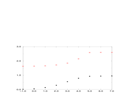
Figure 1: Numerical simulation for $N=1000$ . Horizontal axis is $\lambda$. Stars indicate root mean squares of the eigenvalues and dots indicate the ratio of 16-fold bonds. For large values of $\lambda$, the system is in a BP phase. For small values of $\lambda$, it is in a droplet phase.

The nature of the transition is not clear at the present stage, although it has a similarity to the liquid-gas transition since we have no order parameter associated with a symmetry. The points distribute in full ten dimensions both in these two phases. Other possible interactions such as angle dependent interactions will modify these phases and we may obtain a phase with lower dimensionality.

Finally in this subsection we see what happens if we do not have the core potential. In this case we can use mean field approximation to determine one-particle density in the following way. Let us denote $p_{n}$ as the probability that a point is connected to $n$ other points. Then the self consistent equation for one-particle density is given by

$$\rho(x)={1\over Z}\exp\left(\sum_{n=1}^{\infty}p_{n}n\int\ln(f(x-y))\rho(y)d^{d}y\right),$$

$$\int\rho(x)d^{d}x=1,$$ (3.10)

where $f(x)$ is the Boltzmann factor for each bond and given by $(x^{2}+g)^{-6}$ in our case. Since $N$ does not appear in these equations, the one-particle density does not depend on $N$. Hence all points are condensed into a finite area $V$ which does not depend on $N$. We call this state a mean-field state. We can find a lower bound of the partition function by replacing the length of each bond with the size of the whole system:

$$Z_{\rm MF}>(N!\alpha_{c}^{N})^{2}(V^{-12N/d})^{2}V^{N}e^{-\lambda N_{8}/2}.$$ (3.11)

Since eq. (3.11) contains extra $N!$ compared with $Z_{\rm BP}$ in eq. (3.6), we have to increase $\lambda$ as $\log N\rightarrow\infty$ in order to keep the state in BP phase. Thus we find that any state falls into a mean-field phase if we do not have the core potential.

3.3 A mechanism favoring lower dimensions

Although the double tree model has taught us a lot about the IIB matrix model, we may need to extend it in order to be more faithful to our effective action. As we saw in subsection 3.1, the interaction of 8-fold bonds generally depends on the relative angles of the vectors $x^{ij}_{\mu}$. If eigenvalues extend in ten dimensions, averaging over directions gives a suppression factor to each 8-fold bond, because the tensor $V_{\mu\nu\lambda\rho}$ is traceless. This suppression becomes weak if eigenvalues collapse into lower dimensions. Therefore if there are considerable number of 8-fold bonds, the partition function is suppressed in higher dimensions. However the entropy which is associated with possible orientations of bonds favors higher dimensions. Therefore there is a competition between the two and it is conceivable that four dimensional space-time is realized as a compromise. In what follows we roughly estimate the partition function assuming that the system is in a droplet phase and show the possibility of this scenario.

Assuming that $x^{ij}_{\mu}$ lie isotropically in a $d$ dimensional subspace, we can estimate the orientation average of $V^{ij}_{\mu\nu\lambda\rho}$ as

$$V^{ij}_{\mu\nu\lambda\rho} \sim \left({2(x^{ij})^{4}\over d(d+4)}-{(x^{ij})^{4}\over(d+2)(d+4)}\right)(\hat{\delta}_{\mu\nu}\hat{\delta}_{\lambda\rho}+\hat{\delta}_{\mu\lambda}\hat{\delta}_{\nu\rho}+\cdot\cdot\cdot)$$ (3.12)

$$-{(x^{ij})^{4}\over d(D+4)}(\hat{\delta}_{\mu\nu}{\delta}_{\lambda\rho}+\hat{\delta}_{\mu\lambda}{\delta}_{\nu\rho}+\cdot\cdot\cdot)$$

$$+{(x^{ij})^{4}\over(D+2)(D+4)}(\delta_{\mu\nu}\delta_{\lambda\rho}+\delta_{\mu\lambda}\delta_{\nu\rho}+\cdot\cdot\cdot).$$

Here $\hat{\delta}$ stands for the projection operator to the $d$ dimensional space-time while $\delta$ is the Kronecker’s delta in the original $D=10$ dimensions. The interactions of 8-fold bonds in general involve many $V_{\mu\nu\lambda\rho}$’s whose Lorentz indices are contracted in various ways. It is not easy to estimate the combinatorics which come out from such contractions exactly even after such simplification as eq. (3.12). It may be qualitatively valid to replace $\hat{\delta}$ by ${\delta}$. Then the relevant combinatorics become independent of $d$. Under such an approximation, each 8-fold bond becomes to have a wight effectively which is proportional to

$$e^{-\lambda/2}\sim f_{\rm eff}(d)=\left({1\over(D+2)(D+4)}-{1\over(d+2)(d+4)}+{2\over d}\left({1\over d+4}-{1\over D+4}\right)\right).$$ (3.13)

The weight $f_{\rm eff}(d)$ is a decreasing function and favors lower dimensions. Competition between this weight and entropy which favors higher dimensions determines space-time dimensions in this scenario. If we assume that all bonds are 8-fold and the entropy per bond increases as $d^{\gamma}$, the partition function for a droplet can be expressed as

$$Z_{\rm droplet}=N!e^{-2NF(d)}\sim N!(f_{\rm eff}(d))^{2N}d^{2\gamma N}.$$ (3.14)

The free energy $F$ has a minimum at $d=4$ when $\gamma$ is between 2.6 and 3.1. Fig. 2 shows $F$ as a function of $d$. If this is the mechanism to generate our space-time, we need to determine detailed numerical factors to prove it. We stress here that the model is already fixed by nature and we don’t have freedom to tune parameters.

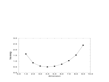
Figure 2: Free energy as a function of dimensions. We take $\gamma=17/6$. Free energy is minimized at four dimensions.

3.4 Other mechanisms for understanding space-time structure

There are two other possible mechanisms to generate lower dimensional structure of the space-time.

One way is to approach from a BP phase in which we regard 8-fold bonds in eq. (3.1) as perturbations to BP’s consisting of 16-fold bonds only. Since Hausdorff dimension of BP is four, there is a possibility that small perturbations might compress the system into four dimensions. If we neglect the effect of self-intersections and naively confine BP into $d$ dimensional space, mean density becomes zero for $d>4$ and diverges for $d<4$ in large $N$ limit. Then for $d<4$, the core potential extends the bond length and energy drastically increases. In other words most of the topologies of BP are prohibited to avoid the increase of energy and the entropy is decreased very much. For $d>4$, large distances between the points prevent 16-fold bonds from resolving into pairs of 8-fold bonds, and we cannot gain the entropy of having 8-fold bonds at various places on the polymer. On the other hand at $d=4$, 8-fold bonds can move around on the polymer and the system behaves as a gas of 8-fold bonds. Therefore only at $d=4$ we can gain the entropy of 8-fold bond gas without too much excess of energy due to the core potential. The mechanism discussed here is based on the picture of BP and seems totally different from the one discussed in subsection 3.3 which is based on the picture of droplet. In four dimensions, however, these two pictures can be complementary, since the size of space-time predicted in these pictures are both $N^{1/4}l$ and agree with each other.

Finally we point out a possibility that four-dimensional space-time is realized in the intermediate region of fig. 1 even for the naive double tree model where dimension dependence of $\lambda$ is not taken into account. Here we consider dimension dependence of the ratio of 8-fold bonds, $r_{8}$. In subsection 3.2 we saw the transition between two limiting phases, namely a BP phase for large $\lambda$ and a droplet phase for small $\lambda$. For intermediate values of $\lambda$, the partition function can be expressed as

$$Z(\lambda)\sim N!\ e^{-N(F(\lambda)+\lambda r_{8})},$$ (3.15)

where $F(\lambda=\infty)=F_{\rm BP}$ and $F(\lambda=-\infty)=F_{\rm droplet}$. Obviously the free energy $F(\lambda)$ defined above is always smaller in higher dimensions. Therefore the system always expands in full dimensions, if $r_{8}$ is independent of dimensions. Our numerical simulations, however, showed that $r_{8}$ is smaller in lower dimensions for fixed values of $\lambda$. It is consistent with the intuition that each point has a smaller number of neighbors in lower dimensions and the probability that two 8-fold bonds coincide to form 16-fold bond is larger. If the dimension dependence of $\lambda r_{8}$ exceeds that of $F(\lambda)$, there is a possibility that lower dimensional phase becomes stabler than the ten dimensional phase for some value of $\lambda$.

4 Conclusions and Discussions

In this concluding section, we first estimate the magnitude of the higher loop contributions to the effective action. Since our expansion parameter is $g^{2}$ over the fourth power of the average distances between the points, long distance behavior is well described by the one-loop effective action $S_{\rm eff}^{\rm 1-loop}[X]$. However there is a possibility that small contributions may pile up at each loop since $N$ color indices circulate around the loop. Our strategy in this section is to assume that the one loop level effective action determines the distribution $\rho(x)$ of the eigenvalues. We then use $\rho(x)$ to estimate the magnitude of the higher loop effects. This procedure is self-consistent if we find that the higher loop effects are small. Of course, our perturbative expansion breaks down if the expansion parameter grows as a positive power of $N$. What we show here is that the higher loop corrections are indeed finite in the large $N$ limit for finite coupling constant, and our approximation based on the loop expansion can be fully justified.

Although we have argued that higher loop effects improve the infrared convergence properties in general, there are diagrams which possess the identical infrared convergence properties with the one loop diagrams in our estimation procedures just explained. For example we may consider the one loop self energy corrections to the propagators of the off-diagonal components. We then consider the insertions of them into the propagators of the one loop diagrams which contribute to the effective action. It is a part of the two loop level contributions.

Recall that the matrix model (1.1) has been constructed by the large $N$ reduction procedure from the $SU(N)$ gauge theory. Thus, in the leading order in $1/N$ expansion, the perturbative expansions in $g^{2}$ in the matrix model are identical to those in the gauge theory were it not for the fermionic zeromodes. They are precisely the part of the quantum corrections we quoted above. Then the ratio of $(l+1)$-loop contributions to $l$-loop contributions may be estimated by dimensional analysis as

$$R_{g^{2}} = g^{2}\sum_{k}\frac{1}{(x^{i}-x^{k})^{4}}$$ (4.1)

$$= g^{2}N\frac{\sum_{k}(x^{i}-x^{k})^{-4}}{\sum_{k}1}$$

$$= g^{2}N\frac{\int d^{10}x\;\rho(x)x^{-4}}{\int d^{10}x\;\rho(x)},$$

where $\rho(x)=\sum_{k}\delta(x-x^{k})$ is a single-particle distribution of the eigenvalues.

We first assume that $x$ is distributed uniformly in a $d$ dimensional manifold with size $R$. From the correspondence with gauge theories, we can say that there is no divergences from small $x$ regions in $d>4$, and from large $x$ regions in $d<4$. Thus,

$$\int^{R}d^{d}x\;x^{-4}=\left\{\begin{array}[]{ll}R^{d-4}&d>4\\ l^{d-4}&d<4\end{array}\right.,$$ (4.2)

where $l$ is a typical size of short distance cutoff. Therefore,

$$R_{g^{2}}=\left\{\begin{array}[]{ll}\frac{g^{2}N}{R^{4}}=N(\frac{l}{R})^{4}&d>4\\ \frac{g^{2}N}{R^{d}l^{4-d}}=N(\frac{l}{R})^{d}&d<4\end{array}\right.,$$ (4.3)

where we used the fact that the core size is $l\sim g^{1/2}$. Since $N\sim(R/l)^{d}$, we may conclude that the quantum corrections are divergent for $d>4$ but finite for $d<4$ in the large $N$ limit. These arguments seems to imply the logarithmic divergence for $d=4$. However here we need to take into account of supersymmetry. It is well-known that dimensional reduction from ten dimensional super Yang-Mills theory down to four implies ${\cal{N}}=4$ supersymmetry in four dimensions. Furthermore four dimensional super Yang-Mills theory with ${\cal{N}}=4$ supersymmetry is also known to be finite. So we expect that the quantum corrections for $d=4$ case is finite.

We have found a divergence in the above argument for $d>4$. However the situation is totally different if we assume that space-time is branched polymer like for $d>4$. We recall that $R\sim N^{1/4}l$ for such space-time since its Hausdorff dimension is four. If so, the estimation of eq. (4.1) is essentially the same as the four dimensional case, and we may conclude that quantum corrections are finite also for $d>4$. Thus we can show that the corrections coming from planner diagrams are finite in the large $N$ limit if the coupling $g^{2}$ is kept fixed.

Next let us consider higher order effects of $1/N$ expansion. It is clear that the leading $1/N^{2}$ corrections contain two less summations over color indices compared with the planar contributions. However they do contribute since they are at least finite. In fact they can be of the same orders of magnitude with the planar contributions since they are more singular at small $x$ regions. For example let us consider a three loop correction to the gluon self-energy. Such a nonplanar contribution should go like

$$g^{6}\sum_{k}{1\over(x^{i}-x^{j})^{6}}{1\over(x^{i}-x^{k})^{2}}{1\over(x^{j}-x^{k})^{4}}.$$ (4.4)

Here the important point is that the superficial degree of divergence for the integration variable $x^{k}$ is reduced compared with that of the corresponding planar diagram. For dimensions up to four, the above expression may be evaluated as follows:

$$g^{6}N{\int d^{10}x\rho(x){1\over(x^{i}-x^{j})^{6}}{1\over(x^{i}-x)^{2}}{1\over(x^{j}-x)^{4}}\over\int d^{10}x\rho(x)}$$ (4.5)

$$= g^{6}N{1\over l^{12-d}R^{d}},$$

where we set $(x^{i}-x^{j})=l\sim g^{1/2}$ to estimate the magnitude of the correction at short distances. Since $N\sim(R/l)^{d}$, the contribution is again nonvanishing and finite in the large $N$ limit.

Therefore infinite numbers of diagrams contribute in dimensions up to four. This means that all orders of $1/N$ expansion contribute equally. On the other hand the nonplanar contributions diverge in general for $d>4$ although they are much smaller compared with the planar contributions unless space-time is branched polymer like. If the space-time is branched polymer like, the situation is essentially identical to the four dimensional case since its fractal dimension is also four. So we may conclude that all orders of $1/N$ expansion contribute in all dimensions.

Our findings may be interpreted that $g_{\rm st}\sim 1$ since we have argued that string coupling constant is inversely proportional to $N$ [2]. Apparently the double scaling limit is naturally taken in the IIB matrix model. However our investigations here also imply that the string scale $(\alpha^{\prime})^{2}\sim g^{2}$. It is in disagreement with our previous estimate $(\alpha^{\prime})^{2}\sim g^{2}N$ based on the loop equations. We believe that reexaminations of the loop equations should be able to reconcile this discrepancy.

We also would like to comment on the universality of IIB matrix models. It is clear from the investigations in this section that the renormalizability and finiteness of four dimensional super Yang-Mills theory is crucial to control the quantum corrections in the IIB matrix model. If we were to add higher dimensional terms to the IIB matrix model, we may need to renormalize the theory nonperturbatively. We expect that such a renormalized theory belongs to the same universality class with ours. Therefore we may argue that the IIB matrix model is universal and our Lagrangian may correspond to the fixed point Lagrangian.

In this paper, we have derived an effective action for the IIB matrix model which is valid when the eigenvalues of $A_{\mu}$ are widely separated. It is the effective action in terms of the super coordinates of space-time. It has clearly shown that the theory has no infrared divergences and the universe never disintegrates. The exciting possibility is that we can determine the dimensionality of space-time by studying such an effective action.

There are order $N$ pairwise attractive potentials between the space-time coordinates. Such interactions may be classified into the 16-fold bond and the 8-fold bond types. If there were only the 16-fold bond interactions, the space-time coordinates form branched polymer type configurations with the fractal dimension four which stretch in ten dimensional space-time. Such a distribution of the eigenvalues cannot be considered as continuous space-time. We have found that the closely packed distributions of the eigenvalues can be realized when we take the 8-fold bond interactions into account. Such distributions can be interpreted as continuous space-time. Here the existence of the hard core repulsive potentials between the eigenvalues is also very important. Although more detailed investigations are required to show that four dimensional space-time is realized in this model, we have proposed possible mechanisms to realize the realistic dimensionality.

We believe that what we have already learned from the IIB matrix model is very significant. It is not defined on the fixed background metric but space-time is dynamically determined as the vacuum of this model. The extent and the dimensionality of space-time can be obtained from the eigenvalue distributions of $A_{\mu}$. In this model, the vacuum is not empty and may be classically represented by the diagonal matrices. The matter (for example D-objects) are the local fluctuations which float on the vacuum. In this way the space-time and the matter are inseparable and they determine each other. Note that such a picture never emerges as long as we deal with the effective Lagrangians for a finite number of D-objects.

If four dimensional space-time is generated dynamically, it will be plausible that the space-time has four dimensional Lorentz invariance. Also it will be intrinsically flat. Here the core potential plays an important role to protect the space-time from shrinking. On the other hand long-distance dynamics protects it from expanding infinitely. This means vanishing of the cosmological constant. In our scenario, stability of generated space-time guarantees absence of cosmological constant in an effective theory of gravity, that is, Einstein gravity. If vacuum energy is generated, eigenvalues are rearranged so as to restore stability of space-time. It is dynamically tuned to be zero. The existence of the hardcore repulsive potential at short distances and the infrared finiteness are responsible to achieve this remarkable feat. It does not explicitly depend on the supersymmetry and hence should be independent of whether supersymmetry is spontaneously broken or not. We believe that this fact alone constitutes a major achievement and hence underscores the validity of the IIB matrix model.

We recall the ${\cal N}=2$ SUSY transformations for the zeromodes:

$$\delta^{(1)}\xi = 0,$$

$$\delta^{(1)}x_{\mu} = i\bar{\epsilon_{1}}\Gamma_{\mu}\xi,$$ (4.6)

and

$$\delta^{(2)}\xi = \epsilon_{2},$$

$$\delta^{(2)}x_{\mu} = 0.$$ (4.7)

The linear combinations of the above translations $\tilde{\delta}^{\pm}=\delta^{1}\pm\delta^{2}$ form the ${\cal N}=2$ supersymmetry algebra. The vacuum expectation value of the supersymmetry transformation of $\xi$ must vanish if supersymmetry is not broken by the vacuum. It is clear from eq.(4.7) that the ${\cal N}=2$ supersymmetry of $\tilde{\delta}^{\pm}$ are broken completely. It is in contrast to the D-string case where the half of the supersymmetry can be preserved. If so, this model realizes the vanishing cosmological constant without supersymmetry as we have argued.

It is also possible to write a scenario to obtain realistic gauge groups in this model. Although we have considered the most generic case where all eigenvalues of $A_{\mu}$ are different from each other, we may assume that some of the eigenvalues remain degenerate. Then the vacuum configurations are represented by the block diagonal matrices where each block is $m$ dimensional. Then the gauge group $SU(m)$ is realized (note that $U(1)$ part is used to make the space-time coordinates). It is also possible to realize the standard model gauge group in an analogous way. We may again integrate out the off-diagonal elements and obtain the effective action for the $U(m)$ submatrices. The resultant effective action must closely resemble the gauge theory with the Planck scale cutoff since we have the local gauge invariance as the manifest symmetry of the effective action.

Since we have argued that it is possible to obtain the realistic gauge groups in four dimensions in this model, it is natural to ask to what kind of string compactification it corresponds. It presumably corresponds to the compactification into the interior of $S^{5}$ that is $B^{6}$. It may be possible to play the analogous games with Calabi-Yau compactifications of heterotic string. It is possible to obtain chiral spinors in the fundamental representations of the gauge group in four dimensions from the chiral spinors in the adjoint representations in ten dimensions. For this purpose we need to assume that there is nontrivial gauge field configuration in $B^{6}$ which produces a nontrivial index for the Dirac operator. We immediately think of a two dimensional example such as magnetic vortices. Then the tensor products of three of them are the possible candidates for such nontrivial gauge configurations.

We also note the similarity between our effective Lagrangian and the dynamical triangulation approach for quantum gravity. Due to the existence of the hardcore potential of the Planck scale, the unit cell of the effective action is also the Planck scale. The pairing interaction between the eigenvalues may be identified with the bonds in the dynamical triangulation approach. The integration over the fermionic zeromodes ensures that the model sums the contributions with all possible connectivities of the bonds just like the dynamical triangulation approach. This analogy may be useful to reconstruct the metric out of the IIB matrix model. We also conjecture that the general coordinate invariance is present in this model due to the following reasoning. There is the permutation symmetry $S_{N}$ which permutes the color indices. It is a subgroup of the full gauge group $SU(N)$ and an exact symmetry of our effective action. Since it does not change the density of the eigenvalues, it should be part of the volume preserving diffeomorphism group in the continuum limit. Similar argument has been made in the dynamical triangulation approach. However it suffers from the infamous conformal mode instability while the IIB matrix model is free from such a disease which is again a remarkable merit of this model. So the gauge and the diffeomorphism invariances may be unified into the $SU(N)$ symmetry of the IIB matrix model.

Although the investigation of this model is still in the initial stage, this model turns out to be a finite theory which is free from both short distance and long distance divergences. The existence of such a theory itself is very impressive. It is a manifestly covariant formulation of superstring which enables us to determine the structure of the vacuum, namely space-time. We have argued that it can solve the problems such as the cosmological constant problem which appear to be insurmountable before the advent of it. Therefore we believe that it will reveal further truths concerning the structure of space-time and the matter.

Appendix A Fierz transformation

In this appendix, we investigate the totally symmetric tensors which can be constructed out of a ten dimensional Majorana-Weyl spinor $\xi$. The effective action contains such a term as $trS^{n}$ where $S^{\mu\nu}=\bar{\xi}\Gamma^{\mu\alpha\nu}\xi~{}{x_{\alpha}/x^{4}}$ and $n$ is an even integer up to 8. Therefore we are interested in totally symmetric tensors.

We first point out that the only nonvanishing tensors which are quadratic in $\xi$ are $\bar{\xi}\Gamma^{\mu\nu\lambda}\xi$. Thus the Fierz transformation is performed quite easily, and we obtain the following identities:

$$(\bar{\xi}\Gamma^{\mu\alpha\beta}\xi)(\bar{\xi}\Gamma^{\nu}_{\;\;\alpha\beta}\xi) = 0,$$ (A.1)

$$(\bar{\xi}\Gamma^{\mu\nu\alpha}\xi)(\bar{\xi}\Gamma^{\lambda\rho}_{\;\;\;\;\alpha}\xi) = (\bar{\xi}\Gamma^{\mu\lambda\alpha}\xi)(\bar{\xi}\Gamma^{\nu\rho}_{\;\;\;\;\alpha}\xi)-(\bar{\xi}\Gamma^{\mu\rho\alpha}\xi)(\bar{\xi}\Gamma^{\nu\lambda}_{\;\;\;\;\alpha}\xi).$$ (A.2)

From eq. (A.1) and eq. (A.2), we can prove the following identity:

$$(\bar{\xi}\Gamma^{\mu\alpha}_{\;\;\;\;\beta}\xi)(\bar{\xi}\Gamma^{\nu\beta}_{\;\;\;\;\gamma}\xi)(\bar{\xi}\Gamma^{\lambda\gamma}_{\;\;\;\;\alpha}\xi)=0.$$ (A.3)

proof: Since the first factor of the left-hand side is antisymmetric in $\alpha$ and $\beta$, the other factors can be antisymmetrized as the right-hand side of eq. (A.2). Therefore using eq. (A.2) we have

$${\rm L.H.S.}=-1/2(\bar{\xi}\Gamma^{\mu\alpha}_{\;\;\;\;\beta}\xi)(\bar{\xi}\Gamma^{\nu\lambda}_{\;\;\;\;\gamma}\xi)(\bar{\xi}\Gamma^{\beta\;\;\gamma}_{\;\;\alpha}\xi),$$ (A.4)

and it vanishes after the contractions of $\alpha$ and $\beta$ due to eq. (A.1). (q.e.d.)

Eq. (A.1) shows that any totally symmetric tensor made of four $\xi$ vanishes. Since sixteen $\xi$ form Lorentz singlet, we can see from the “interchange of particles and holes” that any totally symmetric tensor made of twelve $\xi$ must vanish. From eq. (A.3), we can also conclude the absence of the totally symmetric tensors made of six and ten spinors in an analogous way.

Thus we have shown that the totally symmetric tensors made of $\xi$ are exhausted by the following list: $\{1,\;T^{\mu\nu\lambda\rho}=(\bar{\xi}\Gamma^{\mu\alpha}_{\;\;\;\;\beta}\xi)(\bar{\xi}\Gamma^{\nu\beta}_{\;\;\;\;\gamma}\xi)(\bar{\xi}\Gamma^{\lambda\gamma}_{\;\;\;\;\delta}\xi)(\bar{\xi}\Gamma^{\rho\delta}_{\;\;\;\;\alpha}\xi),\;\xi^{16}\}$. It is easily checked that $T^{\mu\nu\lambda\rho}$ is a totally symmetric traceless tensor in the following way. Similar use of eqs. (A.2) and (A.3) to the above gives the antisymmetric part of $T^{\mu\nu\lambda\rho}$ as

$$T^{\mu\nu[\lambda\rho]} = -1/2(\bar{\xi}\Gamma^{\mu\alpha}_{\;\;\;\;\beta}\xi)(\bar{\xi}\Gamma^{\nu\beta}_{\;\;\;\;\gamma}\xi)(\bar{\xi}\Gamma^{\lambda\rho}_{\;\;\;\;\delta}\xi)(\bar{\xi}\Gamma^{\gamma\;\;\delta}_{\;\;\alpha}\xi),$$ (A.5)

$$= 0,$$

and from eq. (A.1) we immediately see that $T^{\mu\nu\lambda}_{\;\;\;\;\;\;\lambda}=0$. Therefore $T^{\mu\nu\lambda\rho}$ is totally symmetric and traceless.

Appendix B SU(2) Matrix Model

In this appendix, we solve supersymmetric $SU(2)$ matrix models in various dimensions, $D=3,4,6,10$:

$$S=-{1\over g^{2}}Tr({1\over 4}[A_{\mu},A_{\nu}][A^{\mu},A^{\nu}]+{1\over 2}{}^{t}{\psi}\alpha^{\mu}[A_{\mu},\psi]),$$ (B.1)

where $A_{\mu}(\mu=0,1,\cdots,D-1)$ and $\psi$ are $2\times 2$ Hermite matrices, and $\psi$ is a spinor in $D$ dimensional super Yang Mills theory. Each spinor consists of $p_{D}$ real components, where $p_{D}$ is 2,4,8, 16 for $D$=3,4,6,10, respectively. We denote $D$-dimensional alpha matrices by $\alpha^{\mu}$’s ($\alpha^{\mu}=\Gamma^{0}\Gamma^{\mu})$ and the first three of them can be represented as follows:

$$\alpha^{i}={\rho^{i}\otimes\mbox{\boldmath$1$}_{p_{D}/2}},$$

$$\rho^{i}=\cases{\mbox{\boldmath$1_{2}$}&for $i$=0\cr\sigma^{1}&for $i$=1\cr\sigma^{3}&for $i$=2}.$$ (B.2)

Performing the integral over fermionic variables gives the pfaffian

$$\hbox{Pf}(\alpha^{\mu}A_{\mu})=\hbox{Pf}(\alpha^{\mu}T^{a}A^{a}_{\mu}),$$ (B.3)

where $T^{a}$ is the generator of $SU(2)$ in the adjoint representation, namely $(T^{a})_{bc}=\epsilon_{bac}$. Now we“rotate” $A_{\mu}$ by Lorentz transformation so that only $A_{0},A_{1}$and $A_{2}$ are nonvanishing. Eq. (B.3) then reduces to the three-dimensional calculation,

$$\bigl{\{}\hbox{Pf}(\rho^{i}T^{a}A^{a}_{i})\bigr{\}}^{p_{D}/2}\sim\bigl{\{}\epsilon_{ijk}\epsilon_{abc}A^{a}_{i}A^{b}_{j}A^{c}_{k}\bigr{\}}^{p_{D}/2},$$ (B.4)

which corresponds to $(\det A)^{p_{D}/2}$ when we regard $A^{a}_{i}$ as a 3$\times$3 matrix.

Next step is the integration over three ten-dimensional vectors $A^{a}_{\mu}$, which we reduce to the integration over three-dimensional vectors. The Jacobian for this reduction is the volume of the parallelepiped spanned by the three vectors, $A^{1},A^{2}$ and $A^{3}$, to the $(D-3)$-th, which is nothing but $|\det A|^{D-3}$.

To estimate the behavior of the integral, we take the following parametrization for three vectors $A^{a}_{i}$,

$$\left(\matrix{r\cr\mbox{\boldmath$0$}\cr}\right),\left(\matrix{a\cr\mbox{\boldmath$y$}\cr}\right),\left(\matrix{b\cr\mbox{\boldmath$z$}\cr}\right),$$ (B.5)

where $y$ and $z$ are two dimensional vectors while $\mathrm{𝟎}$ is two dimensional zero vector. After these considerations, we obtain

$$\int dAd\psi e^{-S}$$ (B.6)

$$= \int drr^{2}dadbd^{2}\mbox{\boldmath$y$}d^{2}\mbox{\boldmath$z$}\bigl{\{}r(\mbox{\boldmath$y$}\times\mbox{\boldmath$z)$}\bigr{\}}^{p_{D}/2}|r(\mbox{\boldmath$y$}\times\mbox{\boldmath$z)$}|^{D-3}$$

$$\times\exp\bigl{(}-\frac{1}{g^{2}}\bigl{[}r^{2}(\mbox{\boldmath$y$}^{2}+\mbox{\boldmath$z^{2}$})+(a\mbox{\boldmath$z$}-b\mbox{\boldmath$y$})^{2}+(\mbox{\boldmath$y$}\times\mbox{\boldmath$z$})^{2}\bigr{]}\bigr{)}.$$

Integrating over $a$ and $b$ yields

$$\int dadbe^{-(a\mbox{\boldmath$z$}-b\mbox{\boldmath$y$})^{2}}=\bigl{(}\mbox{\boldmath$z$}^{2}\mbox{\boldmath$y$}^{2}-(\mbox{\boldmath$z$}\cdot\mbox{\boldmath$y$})^{2}\bigr{)}^{-1/2}=|\mbox{\boldmath$y$}\times\mbox{\boldmath$z$}|^{-1}.$$ (B.7)

Next, let us integrate over $y$ and $z$. For $D$=3 case the integral becomes identically zero, since $\bigl{\{}r(\mbox{\boldmath$y$}\times\mbox{\boldmath$z)$}\bigr{\}}$ takes the both signs. For the remaining dimensions, we can estimate the integration when $r$ is large and small respectively, which suffice the present purpose. When $r$ is large, the first term of the argument of the exponential in eq. (B.6) becomes dominant. We can perform the integrations over $y$ and $z$ by rescaling them as $\mbox{\boldmath$y$}/r$ and $\mbox{\boldmath$z$}/r$. In this way eq. (B.6) is estimated to be

$$\int drr^{-(p_{D}/2+D-3)} = \int r^{D-1}drr^{-(p_{D}/2+2D-4)}$$ (B.8)

$$= \cases{\int r^{3}dr\;r^{-6}&for $D$=4\cr\int r^{5}dr\;r^{-12}&for $D$=6\cr\int r^{9}dr\;r^{-24}&for $D$=10}\qquad(r^{2}\gg g).$$

When $r$ is small, the first term of the argument of the exponential becomes negligible. We can perform the integrations over $y$ and $z$ independently from $r$. Eq. (B.6) is estimated in this case to be

$$\int drr^{2+(p_{D}/2+D-3)} = \int r^{D-1}drr^{p_{D}/2}$$ (B.9)

$$= \cases{\int r^{3}dr\;r^{2}&for $D$=4\cr\int r^{5}dr\;r^{4}&for $D$=6\cr\int r^{9}dr\;r^{8}&for $D$=10}\qquad(r^{2}\ll g).$$

Finally we confirm that the long distance behavior of $r$ integral (B.8) agrees with the result of the perturbative calculation in the text. Recall that the one-loop effective action for $r$ and $\xi$ is written as

$$S_{\rm eff}^{1-{\rm loop}}[r,\xi]=tr\ln(1+S^{\mu\nu}),$$ (B.10)

where

$$S^{\mu\nu}=\bar{\xi}\Gamma^{\mu\alpha\nu}\xi\frac{r_{\alpha}}{r^{4}}\sim\xi^{2}/r^{3}.$$ (B.11)

Thus the integration over $\xi$

$$\int d^{D}rd^{p_{D}}\xi e^{-S_{\rm eff}[r,\xi]}$$ (B.12)

leads to eq. (B.8).

Appendix C Branched polymer

In this appendix we give a brief introduction to thermodynamics of branched polymers (BP) without self-avoiding effect in $D$ dimensions. (see for example [24]). The partition function of BP with $N$ points and $(N-1)$ bonds is given by

$$Z_{N}=\sum_{\rm BP}\int\prod_{i=1}^{N-1}d^{D}x^{i}\prod_{(ij):{\rm bond}}f(x^{i}-x^{j})\prod_{n=1}^{\infty}t_{n}^{\#n},$$ (C.1)

where the summation is taken over all possible topologies of branched polymers. $t_{n}$ denotes a positive weight assigned for the points to which $n$ bonds are connected and $\#n$ denotes the number of such points in a given configuration. The weight function for bonds $f(x)$ can be Fourier transformed as

$$\hat{f}(p)=\int d^{D}xf(x)e^{-ipx}=\hat{f}(0)(1-c_{2}p^{2}+c_{4}p^{4}+\cdot\cdot\cdot),$$ (C.2)

with a positive coefficient $c_{2}$. Since we are interested in the thermodynamic limit where $N$ goes to infinity, we consider a grand canonical partition function:

$$Z=\sum_{N=1}^{\infty}NZ_{N}k_{0}^{(N-1)}.$$ (C.3)

In order to demonstrate the scaling behavior, we consider a two point correlation function. If we pick up a pair of points in a particular configuration, they are uniquely connected by $n$ bonds. If we assume that they are separated by a fixed distance, $n$ varies from a configuration to another. Therefore we can express a two point function in the momentum space as follows:

$$\hat{G}(p,k_{0}) = \int d^{D}(x-y)G(x-y,k_{0})e^{ip(x-y)}$$ (C.4)

$$\propto \sum_{n=1}^{\infty}k_{0}^{n+1}(t_{1}+t_{2}b+{t_{3}\over 2!}b^{2}+\cdot\cdot\cdot)^{2}(\hat{f}(p))^{n}B^{n-1}.$$

A graphical illustration of this equation is given in fig.3.

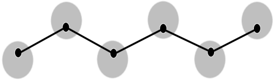
Figure 3: Graphical representation of a two point function. A pair of points in a given configuration can be connected by bonds in a unique way. In this figure they are connected by five bonds. Such bonds form a random walk type object. The remaining points in a branched polymer are connected to the points in this object. They are represented by the blobs in this figure.

The factor $(t_{1}+t_{2}b+\cdot\cdot\cdot)$ is the contribution from each end point in fig. 3. $B$ represents each blob in fig. 3 except those at the end points.

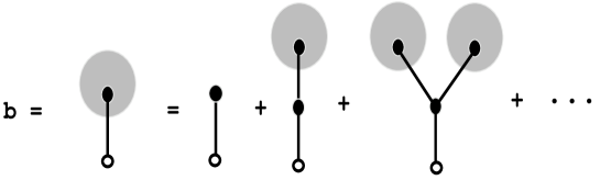
Figure 4: Graphical representation of the Schwinger Dyson equation for $b$. White circles is not associated with any wight.

$b$ is graphically represented in fig.4. It satisfies the following Schwinger Dyson equation

$$b=k_{0}\hat{f}(0)(t_{1}+t_{2}b+{t_{3}\over 2!}b^{2}+\cdot\cdot\cdot)=kh(b),$$ (C.5)

where $k=k_{0}\hat{f}(0)$. The blob $B$ can be related to $h(b)$ as

$$B=t_{2}+t_{3}b+{t_{4}\over 2!}b^{2}+\cdot\cdot\cdot=h^{\prime}(b).$$ (C.6)

From these considerations, we can see that $\hat{G}(p,k_{0})$ can be written as

$$\hat{G}(p,k_{0})\propto{k_{0}^{2}h(b)^{2}\hat{f}(p)\over 1-k_{0}\hat{f}(p)h^{\prime}(b)}.$$ (C.7)

We also note that $Z^{\prime}(b)=h(b)$, since the partition function (C.3) is given by

$$Z(b)=1+t_{1}b+t_{2}b^{2}/2!+t_{3}b^{2}/3!+\cdot\cdot\cdot.$$ (C.8)

Since the averaged number of the points in the branched polymer is given by

$$\bar{N}\sim{k\over Z}{\partial Z\over\partial k}={kh(b)\over Z(b)\left({\partial k\over\partial b}\right)},$$ (C.9)

we must tune the fugacity $k_{0}$ so that $\partial k/\partial b$ approaches zero from a positive value. Eq. (C.5) solves $k$ as a function of $b$: $k=b/h(b)$. A typical solution is illustrated in fig.5.

Figure 5: Typical relation between $k$ and $b$ is drawn. A black dot in the figure indicates the critical point. The large $N$ limit is taken by approaching this point from the left.

Generally $t_{1}\neq 0$ and some of $t_{n}$’s with $n$ larger than 2 are non-zero. We observe that $k(b)$ vanishes at $b=0$ and $b=\infty$. Since it is positive definite, there is a critical fugacity $k_{c}$ where an averaged number becomes infinite.

Near the critical point, $k(b)$ can be approximated by

$$k\sim k_{c}-{c\over 2}(b-b_{c})^{2},$$ (C.10)

where $c$ is a positive constant determined by the set of $t_{n}$’s. The partition function is given by the integral of $h(b)$ over $b$ and it behaves near the critical point as

$$Z={\rm const.}-{b_{c}\over k_{c}}\sqrt{{2(k_{c}-k)\over c}}.$$ (C.11)

The universal part (the second term) determines the power $-3/2$ in the following expansion:

$$Z=\sum_{N=1}^{\infty}N^{-3/2}\left({k\over k_{c}}\right)^{N}\sim\sum_{N=1}^{\infty}N^{-3/2}e^{-{k_{c}-k\over k_{c}}N}.$$ (C.12)

This is because the universal part of the infinite sum of the r.h.s. in eq. (C.12) can be estimated by an integral $\int dNN^{-3/2}exp(-(k_{c}-k)N/k_{c})$. Therefore partition function for a fixed $N$ is $Z_{N}=N^{-3/2}(\hat{f(0)}/k_{c})^{N}$. The leading non-universal behavior is given by

$$Z_{N}\sim(\hat{f(0)}\alpha_{c})^{N},$$ (C.13)

where $\alpha_{c}=1/k_{c}$ takes a value of order one. In a special case where $t_{n}=1$ for all $n$, we find that $k=be^{-b}$ and the critical values are $k_{c}=1/e$ and $b_{c}=1$. This is the case relevant to our analysis.

Inserting $kh^{\prime}(b)=1-h(b)k^{\prime}(b)$ (which is derived from eq. (C.5)) into eq. (C.7), we obtain a scaling behavior of a two point function near the critical point. For small $p$, it behaves as

$$\hat{G}(p,k_{0}) \propto {k_{0,c}^{2}h^{2}(b_{c})\hat{f}(p)\over 1-(\hat{f}(p)/\hat{f}(0))(1-\sqrt{2c(k_{c}-k)}h(b_{c}))}$$ (C.14)

$$\propto {1\over p^{2}+M^{2}\sqrt{(k_{c}-k)}}\propto{1\over(p_{phy}^{2}+M^{2})\sqrt{(k_{c}-k)}}$$

where $M^{2}=\sqrt{2c}h(b_{c})/c_{2}$. In order to take a scaling limit, we have introduced the physical momentum $p_{phy}=p(k_{c}-k)^{-1/4}$. In this way, we have obtained the scaling relation:

$$(k_{c}-k)^{-1/2}G(x(k_{c}-k)^{-1/4},k_{0})\stackrel{{\scriptstyle k\rightarrow k_{c}}}{{\longrightarrow}}g(x)$$ (C.15)

where $g(x)$ is a certain function. Since the dominant contribution comes from $N\sim k_{c}/(k_{c}-k)$, we can observe from eq. (C.15) that the Hausdorff dimension of a branched polymer is four.

References

- [1] N. Ishibashi, H. Kawai, Y. Kitazawa and A. Tsuchiya, A Large-N Reduced Model as Superstring, Nucl. Phys. B498 (1997) 467; hep-th/9612115.
- [2] M. Fukuma, H. Kawai. Y. Kitazawa and A. Tsuchiya, String Field Theory from IIB Matrix Model, hep-th/9705128, to appear in Nucl. Phys. B.
- [3] T. Banks, W. Fischler, S.H. Shenker and L. Susskind, M Theory as a Matrix Model: a Conjecture, Phys. Rev. D55 (1997) 5112; hep-th/9610043.
- [4] M. Green and J. Schwarz, Phys. Lett. 136B (1984) 367.
- [5] A. Schild, Phys. Rev. D16 (1977) 1722.
- [6] E. Witten, Nucl. Phys. B443 (1995) 85.
-
[7]
T. Eguchi and H. Kawai, Phys. Rev. Lett. 48 (1982) 1063.
G. Parisi, Phys. Lett. 112B (1982) 463.
D. Gross and Y. Kitazawa, Nucl. Phys. B206 (1982) 440.
G. Bhanot, U. Heller and H. Neuberger, Phys. Lett. 113B (1982) 47.
S. Das and S. Wadia, Phys. Lett. 117B (1982) 228.
J. Alfaro and B. Sakita, Phys. Lett. 121B (1983) 339. - [8] V. Periwal Matrices on a Point as the Theory of Everything, hep-th/9611103.
- [9] M. Li, Strings from IIB Matrices, hep-th/961222.
- [10] I. Chepelev, Y. Makeenko and K. Zarembo, Properties of D-branes in Matrix Model of IIB Superstring, hep-th/9701151.
- [11] A. Fayyazuddin and D.J. Smith, P-Brane Solutions in IKKT IIB Matrix Theory, hep-th/9701168.
- [12] A. Fayyazuddin , Y. Makeenko, P. Olesen, D.J. Smith and K. Zarembo, Towards a Non-perturbative Formulation of IIB Superstrings by Matrix Models, hep-th/9703038.
- [13] T. Yoneya, Schild Action and Space-Time Uncertainty Principle in String Theory, hep-th/9703078.
- [14] C. F. Kristjansen and P. Olesen, A Possible IIB Superstring Matrix Model with Euler Characteristic and a Double Scaling Limit, hep-th/9704017.
- [15] I. Chepelev and A. A. Tseytlin, Interaction of type IIB D-branes from D-instanton Matrix Model, hep-th/9705120.
- [16] S. Hirano and M. Kato, Topological Matrix Model, hep-th/9708039.
- [17] H. Itoyama, A. Tokura, USp(2k) Matrix Model: F theory Connection, hep-th/9708123; USp(2k) Matrix Model: Nonperturbative Approach to Orientifolds, hep-th/9801084.
- [18] B. P. Mandal and S. Mukhopadhyay, D-brane Interaction in the type IIB Matrix Model, hep-th/9709098.
- [19] N. D. Hari Dass and B. Sathiapalan, Interaction of F strings and D strings in the Matrix Model, hep-th/9712179.
- [20] I. Oda, Matrix Theory from Schild Action, hep-th/9801085.
-
[21]
A. Connes, Gravity coupled with matter and the
formulation of
non commutative geometry, Comm. Math. Phys. 182 (1996) 155; hep-th/9603053.
A. Connes, M. Douglas and A. Schwarz, Noncommutative Geometry and Matrix Theory: Compactification on Tori, hep-th/9711162. - [22] T. Suyama and A. Tsuchiya, Exact Results in IIB Matrix Model, hep-th/9711073.
- [23] S. Sethi and M. Stern, D-Brane Bound States Redux, hep-th/9705046; Piljin Yi, Nucl. Phys. B505 (1997) 307, hep-th/9704098.
- [24] J. Ambjorn, B Durhuus and T. Jonsson, Quantum Geometry, Cambridge (1997).