Brane Dynamics and Gauge Theory

Abstract

We review some aspects of the interplay between the dynamics of branes in string theory and the classical and quantum physics of gauge theories with different numbers of supersymmetries in various dimensions.

Contents

toc

I Introduction

Non-abelian gauge theories are a cornerstone of the standard model of elementary particle physics. Such theories (for example QCD) are often strongly coupled at long distances and, therefore, cannot be studied by the standard perturbative methods of weakly coupled field theory. In the last few years important progress was made in the study of the strongly coupled dynamics in a class of gauge theories – Supersymmetric Yang-Mills (SYM) theories. New understanding of the constraints due to supersymmetry, the importance of solitonic objects and electric-magnetic, strong-weak coupling duality, led to many exact results on the vacuum structure of various supersymmetric field theories.

Despite the fact that supersymmetry (a symmetry relating bosons and fermions) is not present in the standard model, there are at least three reasons to study supersymmetric gauge theories:

• It is widely believed that an $N=1$ supersymmetric extension of the standard model describes physics at energies not far above those of current accelerators, and is directly relevant to the hierarchy problem and unification of couplings.

• Supersymmetric gauge theories provide examples of many phenomena believed to occur in non-supersymmetric theories in a more tractable setting. Therefore, they serve as useful toy models for the study of these phenomena.

• The study of supersymmetric field theories has many mathematical applications.

Non-abelian gauge theories also appear in low energy approximations to string theory, where supersymmetry plays an important role. String theory is a theory of quantum gravity which, moreover, unifies gravity and gauge fields in a consistent quantum theory. Traditionally, the theory has been formulated in an expansion in a (string) coupling, however, many of the outstanding problems in the subject have to do with physics outside the weak coupling domain. String theory has also been undergoing rapid progress in the last few years, which was driven by similar ideas to those mentioned in the gauge theory context above.

Some of the highlights of the progress in gauge and string theory that are relevant for this review are:

1. Strong-Weak Coupling Duality

The physics of asymptotically free gauge theory depends on the energy scale at which the theory is studied. At high energies the theory becomes weakly coupled and is well described in terms of the fundamental fields in the Lagrangian (such as quarks and gluons). At low energies the theory is often strongly coupled and can exhibit several different behaviors (or phases): confining, Higgs, Coulomb, free electric and free magnetic phases.

In the confining phase, the energy of a pair of test charges separated by a large distance $R$ grows linearly with $R$. Thus, such charges cannot be infinitely separated. In the Higgs phase, the gauge bosons are massive and the energy of a pair of test charges goes to a constant at large $R$. The Coulomb phase is characterized by potentials that go like $1/R$, while the free electric and magnetic phases have logarithmic corrections to this behavior. The standard model of elementary particle physics realizes the confining, Higgs and free electric phases; other models that go beyond the standard model use the other phases as well.

The determination of the phase structure of non-abelian gauge theories is an important problem that is in general complicated because it involves understanding the physics of strongly coupled gauge theory. In the last few years, this problem has been solved for many supersymmetric gauge theories. One of the main advances that led to this progress was the realization that electric-magnetic, strong-weak coupling duality is quite generic in field theory.

In a typical realization of such a duality, one studies an asympotitcally free gauge theory that becomes more and more strongly coupled as one goes to lower and lower energies. The extreme low energy behavior is then found to be governed by a different theory which may be weakly coupled, e.g. because it is not asymptotically free.

In other interesting situations, the original theory depends on continuous parameters (exactly marginal deformations), and the duality relates the theory at different values of these parameters. An example of this is the maximally supersymmetric four dimensional gauge theory, $N=4$ SYM. This theory depends on a complex parameter $\tau$, whose imaginary part is proportional to the square of the inverse gauge coupling; the real part of $\tau$ is a certain $\theta$ angle. The theory becomes weakly coupled when ${\rm Im}\tau\to\infty$. It has been proposed that it is invariant under a strong-weak coupling duality $\tau\to-1/\tau$ in addition to the semiclassically manifest symmetry $\tau\to\tau+1$. This symmetry is a generalization of the well known symmetry of electrodynamics which takes $\vec{E}\to\vec{B}$ and $\vec{B}\to-\vec{E}$ and at the same time exchanges electric and magnetic charges. In the last few years convincing evidence has been found for the validity of this duality symmetry of $N=4$ SYM.

Many interesting generalizations to theories with less supersymmetry have been found. For example, certain “finite” supersymmetric gauge theories (e.g. $N=2$ SYM with gauge group $SU(N_{c})$ and $N_{f}=2N_{c}$ “flavors” of fundamental hypermultiplets) also appear to have such symmetries. Furthermore, it has been discovered that different $N=1$ supersymmetric gauge theories may flow to the same infrared fixed point and thus exhibit the same long distance behavior. As we change the parameters defining the different theories, one of the descriptions might become more weakly coupled in the infrared while another might become more strongly coupled. In some cases, this equivalence relates a strongly coupled interacting gauge theory to an infrared free one. Interesting phenomena have also been shown to occur in other dimensions; in particular, a large class of previously unsuspected non-trivial fixed points in five and six dimensional field theory has been found.

String theory has been known for a long time to be invariant under a large discrete symmetry group known as T-duality. This duality relates weakly coupled string theories and is valid order by order in the string coupling expansion. It relates different spacetime backgrounds in which the string propagates. A simple example of T-duality is the equivalence of string propagation on a circle of radii $R$ and $1/R$. A perturbative fundamental string state that carries momentum $n/R$ around the circle is mapped by T-duality to a perturbative fundamental string state corresponding to a string winding $n$ times around the dual circle of radius $1/R$.

In the last few years it has been convincingly argued that the perturbative T-duality group is enhanced in the full string theory to a larger symmetry group, known as U-duality, which relates perturbative string states to solitons, and connects different string vacua that were previously thought of as distinct theories. In certain strong coupling limits string theory becomes eleven dimensional and is replaced by an inherently quantum “M-theory.” At low energies M-theory reduces to eleven dimensional supergravity; the full structure of the quantum theory is not well understood as of this writing.

2. Solitonic Objects

Gauge theories in the Higgs phase often have solitonic solutions that carry magnetic charge. Such monopoles and their dyonic generalizations (which carry both electric and magnetic charge) play an important role in establishing duality in gauge theory. In supersymmetric gauge theories their importance is partly due to the fact that they preserve some supersymmetries and, therefore, belong to special representations of the supersymmetry algebra known as “short” multiplets, which contain fewer states than standard “long” multiplets of the superalgebra. Particles that preserve part of the supersymmetry are conventionally referred to as being “BPS saturated.” Because of the symmetries, some of the properties of these solitons can be shown to be independent of the coupling constants, and thus certain properties can be computed exactly by weak coupling methods. Often, at strong coupling, they become the light degrees of freedom in terms of which the long distance physics should be formulated.

In string theory analogous objects were found. These are BPS saturated $p$-branes, $p$ dimensional objects (with $p+1$ dimensional worldvolumes) which play an important role in establishing U-duality. In various strong coupling regions different branes can become light and/or weakly coupled, and serve as the degrees of freedom in terms of which the dynamics should be formulated. The study of branes preserving part of the supersymmetry in string theory led to fascinating connections, some of which will be reviewed below, between string (or brane) theory and gauge theory.

3. Quantum Moduli Spaces Of Vacua

SYM theories and string theories often have massless scalar fields with vanishing classical potential and, therefore, a manifold of inequivalent classical vacua ${\cal M}_{cl}$, which is parametrized by constant expectation values of these scalar fields. In the non-supersymmetric case quantum effects generically lift the moduli space ${\cal M}_{cl}$, leaving behind a finite number of quantum vacua. In supersymmetric theories the quantum lifting of the classical moduli space is severely constrained by certain non-renormalization theorems. The quantum corrections to the scalar potential can often be described by a dynamically generated non-perturbative superpotential , which is severely restricted by holomorphicity, global symmetries and large field behavior. One often finds an unlifted quantum moduli space ${\cal M}_{q}$. In many gauge theories the quantum superpotentials were analyzed and the moduli spaces ${\cal M}_{q}$ have been determined. Partial success was also achieved in the analogous problem in string theory.

Branes have proven useful in relating string dynamics to low energy phenomena. In certain limits brane configurations in string theory are well described as solitonic solutions of low energy supergravity, in particular black holes. Interactions between branes are then mainly due to “bulk” gravity. In other limits gravity decouples and brane dynamics is well described by the light modes living on the worldvolume of the branes. Often, these light modes describe gauge theories in various dimensions with different kinds of matter. Studying the brane description in different limits sheds new light on the quantum mechanics of black holes, as well as quantum gauge theory dynamics. Most strikingly, both subjects are seen to be different aspects of a single problem: the dynamics of branes in string theory.

The fact that embedding gauge theories in string theory can help analyze strongly coupled low energy gauge dynamics is a priori surprising. Standard Renormalization Group (RG) arguments would suggest that at low energies one can integrate out all fluctuations of the string except the gauge theory degrees of freedom, which are governed by SYM dynamics (gravity also decouples in the low energy limit). This would seem to imply that string theory cannot in principle teach us anything about low energy gauge dynamics.

Recent work suggests that while most of the degrees of freedom of string theory are indeed irrelevant for understanding low energy physics, there is a sector of the theory that is significantly larger than the gauge theory in question that should be kept to understand the low energy structure. This sector involves degrees of freedom living on branes and describing their internal fluctuations and embedding in spacetime.

We will see that the reasons for the “failure” of the naive intuition here are rather standard in the general theory of the RG:

1. In situations where the long distance theory exhibits symmetries, it is advantageous to study RG trajectories along which the symmetries are manifest (if such trajectories exist). The string embedding of SYM often provides such a trajectory. Other RG trajectories (e.g. the standard QFT definition of SYM in our case) which describe the same long distance physics may be less useful for studying the consequences of these symmetries, since they are either absent throughout the RG flow, arising as accidental symmetries in the extreme IR limit, or are hidden in the variables that are being used.

2. Embedding apparently unrelated low energy theories in a larger high energy theory can reveal continuous deformations of one into the other that proceed through regions in parameter space where both low energy descriptions fail.

3. The embedding in string theory allows one to study a much wider class of long distance behaviors than is possible in asymptotically free gauge theory.

In brane theory, gauge theory arises as an effective low energy description that is useful in some region in the moduli space of vacua. Different descriptions are useful in different regions of moduli space, and in some regions the extreme IR behavior cannot be given a field theory interpretation. The underlying dynamics is always the same – brane worldvolume dynamics in string theory. Via the magic of string theory, brane dynamics provides a uniform and powerful geometrical picture of a diverse set of gauge theory phenomena and points to hidden relations between them.

The purpose of this review is to provide an overview of some aspects of the rich interplay between brane dynamics and supersymmetric gauge theory in different dimensions. We tried to make the presentation relatively self contained, but the reader should definitely consult reviews (some of which are listed below) on string theory, D-branes, string duality, and the recent progress in supersymmetric gauge theory, for general background and more detailed discussions of aspects that are only mentioned in passing below.

A General References

In the last few years there was a lot of work on subjects relevant to this review. Below we list a few of the recent original papers and reviews that can serve as a guide to the literature.

We use the following “conventions” in labeling the references: for papers with up to three authors we list the authors’ last names in the text; if there are more than three authors, we refer to the paper as “First author et al.” For papers which first appeared as e-prints, the year listed is that of the e-print; papers before the e-print era are labeled by the publication year. In situations where the above two conventions do not lift the degeneracy we assign labels “a,b,c,…”

For introductions to SUSY field theory see for example [103, 231]. Electric-magnetic strong-weak coupling duality in four dimensional gauge theory dates back to the work of [169]. Reviews of the exact duality in $N=4$ SYM and additional references to the literature can be found in [180, 127, 76]. [127] also includes a pedagogical introduction to magnetic monopoles and other BPS states.

The recent progress in $N=2$ SYM started with the work of [208, 209]. Reviews include [48, 76, 163, 22]. The recent progress in $N=1$ SUSY gauge theory was led by Seiberg; two of the important original papers are [200, 201]. Some reviews of the work on $N=1$ supersymmetric theories are [23, 202, 139, 109, 184, 216].

The standard reference on string theory is [117]; for a recent review see [148]. Dirichlet branes are described in [186, 188, 187]. Solitonic branes are discussed in [59]. A comprehensive review on solitons in string theory is [84].

T-duality is reviewed in [111]. The non-perturbative dualities and M-theory are discussed in [135, 233, 196, 197, 222, 226, 223] and many additional papers. A recent summary for non-experts is [198]. Finally, reviews on applications of branes to black hole physics can be found, for example, in [166, 241, 183].

B Plan

The plan of the review is as follows. In section II we introduce the cast of characters – the different $1/2$ BPS saturated branes in string theory.

We start, in section II A, by describing the field content of ten and eleven dimensional supergravity and, in particular, the $p$-form gauge fields to which different branes couple. In section II B we describe different branes at weak string coupling, where they appear as heavy non-perturbative solitons charged under various $p$-form gauge fields. This includes Dirichlet branes (D-branes) which are charged under Ramond sector gauge fields and solitonic branes charged under Neveu-Schwarz sector gauge fields. We also describe orientifolds, which are non-dynamical objects (at least at weak string coupling) that are very useful for applications to gauge theory.

In section II C we discuss the interpretation of the different branes in M-theory, the eleven dimensional theory that is believed to underlie all string vacua as well as eleven dimensional supergravity. We show how different branes in string theory descend from the membrane and fivebrane of M-theory, and discuss the corresponding superalgebras.

In section II D we describe the transformation of the various branes under U-duality, the non-perturbative discrete symmetry of compactified string (or M-) theory. In section II E we initiate the discussion of branes preserving less than $1/2$ of the SUSY, with particular emphasis on their worldvolume dynamics. We introduce configurations of branes ending on branes that are central to the gauge theory applications, and discuss some of their properties.

Section III focuses on configurations of parallel Dirichlet threebranes which realize four dimensional $N=4$ SYM on their worldvolume. We describe the limit in which the worldvolume gauge theory decouples from all the complications of string physics and explain two known features of $N=4$ SYM using branes. The Montonen-Olive electric-magnetic duality symmetry is seen to be a low energy manifestation of the $SL(2,Z)$ self-duality of ten dimensional type IIB string theory; Nahm’s description of multi-monopole moduli space is shown to follow from the realization of monopoles as D-strings stretched between $D3$-branes preserving $1/2$ of the SUSY. We also describe the form of the metric on monopole moduli space, and some properties of the generalization to symplectic and orthogonal groups obtained by studying threebranes near an orientifold threeplane.

In section IV we move on to brane configurations describing four dimensional $N=2$ SYM. In particular, in section IV C we explain, using a construction of branes suspended between branes, the observation by Seiberg and Witten that the metric on the Coulomb branch of such theories is given by the period matrix of an auxiliary Riemann surface $\Sigma$. In the brane picture this Riemann surface becomes physical, and is interpreted as part of the worldvolume of a fivebrane. $N=2$ SYM is obtained in brane theory by studying the worldvolume theory of the fivebrane wrapped around $R^{3,1}\times\Sigma$. We also discuss the geometrical realization of the Higgs branch and various deformations of the theory.

Section V is devoted to four dimensional theories with $N=1$ SUSY. We describe the classical and quantum phase structure of such theories as a function of the parameters in the Lagrangian, and explain Seiberg’s duality between different theories using branes. In the brane construction, the quantum moduli spaces of members of a dual pair provide different parametrizations of a single space – the moduli space of the corresponding brane configuration. Each description is natural in a different region in parameter space. Seiberg’s duality in brane theory is thus reminiscent of the well known correspondence between two dimensional sigma models on Calabi-Yau hypersurfaces in weighted projective spaces and Landau-Ginzburg models with $N=(2,2)$ SUSY [145, 167, 118], where the relation between the two descriptions can be established by embedding both in the larger framework of the (non-conformal) gauged linear sigma model [232].

In section VI we study three dimensional theories. In section VI A we establish using brane theory two results in $N=4$ SYM. One is that the moduli space of many such theories is identical as a hyper-Kähler manifold to the moduli space of monopoles in a different gauge theory. The other is “mirror symmetry,” i.e. the statement that many $N=4$ SUSY gauge theories have mirror partners such that the Higgs branch of one theory is the Coulomb branch of its mirror partner and vice-versa. In section VI B we study $N=2$ SUSY theories. We describe the quantum moduli space of $N=2$ SQCD using branes and show that the two dualities mentioned above, Seiberg’s duality and mirror symmetry, can be extended to this case and teach us new things both about branes and about gauge theories. We also discuss the phase structure of four dimensional $N=1$ SUSY gauge theory compactified to three dimensions on a circle of radius $R$.

In section VII we consider two dimensional theories. We study $2d$ $N=(4,4)$ supersymmetric theories and compactifications of $N=4$ supersymmetric models from three to two dimensions on a circle. We also discuss $N=(2,2)$ SUSY theories in two dimensions. In section VIII we study some aspects of five and six dimensional theories, as well as compactifications from five to four dimensions on a circle. Finally, in section IX we summarize the discussion and mention some open problems.

C Omissions

In the following we briefly discuss issues that will not be reviewed extensively :

• Gauge Theories in Calabi-Yau Compactifications: An alternative (but related) way to study low energy gauge theory is to compactify string theory to $D$ dimensions on a manifold preserving the required amount of SUSY, and take $M_{Planck}\to\infty$ to decouple gravity and massive string modes. This leads to a low energy gauge theory, some of whose properties can be related to the geometry of the internal space.

  In particular, compacifications of the type II string on singular Calabi-Yau (CY) threefolds – fibrations of ALE spaces over $CP^{1}$ – are useful in the study of $N=2$ SYM theories [143, 150]; for reviews see [163, 149]. BPS states are related to type IIB threebranes wrapped around 3-cycles which are fibrations of vanishing 2-cycles in the ALE space. On the base the threebrane is projected to a self-dual string on a Riemann surface $\Sigma$, which is the Seiberg-Witten curve. The string tension is related to the Seiberg-Witten differential $\lambda$. The existence of stable BPS states is reduced to a geodesic problem on $\Sigma$ with metric $|\lambda|^{2}$.

  Similarly, to study $N=1$ SYM theories in four dimensions one compactifies F-theory [225] on Calabi-Yau fourfolds. This “geometric engineering” was initiated in [146, 147] and is reviewed in [149].

• Probing the Geometry of Branes with Branes: We shall briefly describe a few (related) examples where the geometry near branes can be probed by lighter objects. In particular, we shall describe the metric felt by a fundamental string propagating in the background of solitonic fivebranes, and by threebranes near parallel sevenbranes and orientifold sevenplanes. In the latter case, the geometrical data is translated into properties of the four dimensional $N=2$ supersymetric gauge theory on the threebranes.

  The interplay between the gauge dynamics on branes and the geometry corresponding to the presence of other branes was studied in [78, 211, 33] and was generalized in many directions.

  For instance, fourbranes can be used to probe the geometry of parallel eightbranes and orientifold eightplanes, leading to an interesting connection between five dimensional gauge theory and geometry [204, 170, 80]. Similarly, $p$-branes (with $p<3$) can be used to probe the geometry near parallel $(p+4)$-branes and orientifold $(p+4)$-planes, leading to relations between low dimensional ($D<4$) gauge theories and geometry [203, 210, 74, 35], some of which will be discussed in this review. Other brane configurations that were used to study the interplay between geometry and gauge theory appear in [10, 213, 12, 82, 214].

• Branes in Calabi-Yau Backgrounds: As should be clear from the last two items, there is a close connection between brane configurations and non-trivial string backgrounds. In general one may consider branes propagating in non-trivial backgrounds, such as CY compactifications. The branes may live at points in the internal space or wrap non-trivial cycles of the manifold.

  Such systems are studied for example in [45, 83, 81, 46, 227, 136, 182, 133, 15, 49, 13, 20, 16] and references therein. In some limits, they are related by duality transformations to the webs of branes in flat space that are extensively discussed below [181, 154, 87, 182]. For example, a useful duality, which we shall review below, is the one relating the $A$-type singularity on $K3$ to a configuration of parallel solitonic fivebranes.

• Quantum Mechanics of Systems of $D0$-Branes, D-Instantons, Matrix Theory: The QM of $D0$-branes in type IIA string theory (in general in the presence of other branes and orientifolds) led to fascinating developments which are outside the scope of this review [79, 35, 37, 191, 31]. Matrix theory was introduced in [34]; reviews and additional references are in [32, 47]. D-instantons were studied, for example, in [115, 116] and references therein.

• Non-Supersymmetric Theories: It is easy to construct brane configurations in string theory that do not preserve any supersymmetry. So far, not much was learned about non-supersymmetric gauge theories by studying such configurations (for reasons that we shall explain). Some recent discussions appear in [52, 238, 113, 93, 38]. Dynamical supersymmetry breaking in the brane picture was considered recently in [67].

II Branes In String Theory

In addition to fundamental strings, in terms of which it is usually formulated, string theory contains other extended $p$ dimensional objects, known as $p$-branes, that play an important role in the dynamics. These objects can be divided into two broad classes according to their properties for weak fundamental string coupling $g_{s}$: “solitonic” or Neveu-Schwarz (NS) branes, whose tension (energy per unit $p$-volume) behaves like $1/g_{s}^{2}$, and Dirichlet or D-branes, whose tension is proportional to $1/g_{s}$ (and which are hence much lighter than NS-branes in the $g_{s}\to 0$ limit).

In this section we describe some properties of the various branes. In supergravity, these $p$-branes are charged under certain massless $(p+1)$-form gauge fields. We start with a description of the low energy effective theory corresponding to type II strings in ten dimensions as well as eleven dimensional supergravity, the low energy limit of M-theory. We then describe branes preserving half of the SUSY in weakly coupled string theory: D-branes, orientifold planes, and solitonic and Kaluza-Klein fivebranes. We present the interpretation of the different branes from the point of view of the full quantum eleven dimensional M-theory, and their transformation properties under U-duality. We finish the section with a discussion of webs of branes preserving less SUSY.

Our notations are as follows: the $1+9$ dimensional spacetime of string theory is labeled by $(x^{0},x^{1},\cdots,x^{9})$. The tenth spatial dimension of M-theory is $x^{10}$. The corresponding Dirac matrices are $\Gamma^{M}$, $M=0,1,2,\cdots,10$. Type IIA string theory has $(1,1)$ spacetime supersymmetry (SUSY); the spacetime supercharges generated by left and right moving worldsheet degrees of freedom $Q_{L}$, $Q_{R}$ have opposite chirality:

$$\Gamma^{0}\cdots\Gamma^{9}Q_{L}= +Q_{L}$$ (1)

$$\Gamma^{0}\cdots\Gamma^{9}Q_{R}= -Q_{R}$$ (2)

Type IIB string theory has $(2,0)$ spacetime SUSY, with both left and right moving supercharges having the same chirality:

$$\Gamma^{0}\cdots\Gamma^{9}Q_{L}= Q_{L}$$ (3)

$$\Gamma^{0}\cdots\Gamma^{9}Q_{R}= Q_{R}$$ (4)

Thus, IIA string theory is non-chiral, while the IIB theory is chiral. We will mainly focus on type II string theories, but $1+9$ dimensional theories with $(1,0)$ SUSY can be similarly discussed. Type I string theory can be thought of as type II string theory with orientifolds and D-branes and is, therefore, a special case of the discussion below. Heterotic strings do not have D-branes, but do have NS-branes similar to those described below.

A Low Energy Supergravity

The spectrum of string theory contains a finite number of light particles and an infinite tower of massive excitations with string scale or higher masses. To make contact with low energy phenomenology it is convenient to focus on the dynamics of the light modes. This can be achieved by integrating out the infinite tower of massive fluctuations of the string and defining a low energy effective action for the light fields. If one thinks (formally) of string theory as a theory describing an infinite number of fields $\phi$, some of which are light $\phi_{l}$, and the rest are heavy $\phi_{h}$, governed by the classical action $S(\phi_{l},\phi_{h})$, the low energy effective action $S_{\rm eff}(\phi_{l})$ can in principle be obtained by integrating out the heavy fields:

$$e^{iS_{\rm eff}(\phi_{l})}=\int D\phi_{h}e^{iS(\phi_{l},\phi_{h})}$$ (5)

In principle (5) is exact, but in practice it is far from clear how to find the action $S$ and how to integrate out the massive modes of the string. At the same time, the effective action is mainly of interest at energies much lower than the masses of the fields $\phi_{h}$, where it makes sense to integrate them out. To find $S_{\rm eff}$ at low energies one can study the S-matrix of the string in the low energy approximation and construct a classical action that reproduces it. The leading terms in such an action are typically determined by the symmetries, such as gauge and diffeomorphism invariance, and supersymmetry.

Following the above discussion for type II string theory leads to the two $9+1$ dimensional type II supergravity theories, type IIA and type IIB. Ten dimensional type IIA supergravity can be obtained by dimensional reduction of the unique eleven dimensional supergravity theory, which is of interest in its own right as the low energy limit of M-theory; thus we start with this case.

Eleven dimensional supergravity includes the bosonic (i.e. commuting) fields $G_{MN}$, the eleven dimensional metric, and $A_{MNP}$, a three index antisymmetric gauge field ($M,N,P=0,1,\cdots,10$). The only fermionic field is the gravitino, $\psi^{M}_{\alpha}$ ($\alpha=1,\cdots,32$). The Lagrangian describing these fields can be found in [117]. One can check that there are $128$ on-shell bosonic and fermionic degrees of freedom.

The presence of the three index gauge field $A_{MNP}$ implies that eleven dimensional supergravity couples naturally to membranes and to fivebranes. For a membrane with worldvolume $X^{M}(\sigma_{a})$, ($a=1,2,3$), the coupling is (see [42] for a discussion of the full supermembrane worldvolume action)

$$\int d^{3}\sigma\epsilon^{abc}A_{MNP}(X)\partial_{a}X^{M}\partial_{b}X^{N}\partial_{c}X^{P}$$ (6)

Equation (6) implies that the membrane of eleven dimensional supergravity is charged under the three-form gauge field $A_{MNP}$. The coupling of eleven dimensional supergravity to fivebranes is similar, with $A_{MNP}$ replaced by its dual $\tilde{A}_{MNPQRS}$ defined by $*dA=d\tilde{A}$.

Type IIA supergravity is obtained by dimensional reduction of eleven dimensional supergravity on a circle. Denoting the $1+9$ dimensional indices by $\mu,\nu,\lambda=0,1,\cdots,9$, the fields of eleven dimensional supergravity reduce as follows in this limit. The metric $G_{MN}$ gives rise to the metric $G_{\mu\nu}$, a gauge field $A_{\mu}=G_{\mu,10}$ and a scalar $\Phi=G_{10,10}$. The antisymmetric tensor $A_{MNP}$ similarly gives rise to the antisymmetric tensors $A_{\mu\nu\lambda}$ and $B_{\mu\nu}=A_{\mu\nu,10}$. In the standard Neveu-Schwarz-Ramond quantization of superstrings [117], the fields $G_{\mu\nu}$, $B_{\mu\nu}$ and $\Phi$ originate in the same sector of the string Hilbert space, the Neveu-Schwarz (or NS) sector, while the gauge fields $A_{\mu}$ and $A_{\mu\nu\lambda}$ are Ramond-Ramond (RR) sector fields. The scalar field $\Phi$ is the dilaton; its expectation value determines the coupling constant of the string theory. Since the potential for $\Phi$ in type II string theory vanishes, the theory can be made arbitrarily weakly coupled.

Just like in eq. (6), the existence of the gauge fields implies that type II string theory naturally couples to various $p$-branes. The existence of $B_{\mu\nu}$ means that the theory naturally couples to strings (electrically, as in (6)) and fivebranes (magnetically, via the six-form gauge field dual to $B_{\mu\nu}$). Since the gauge field to which these branes couple is an NS sector field we refer to these branes as NS branes. The string charged under $B_{\mu\nu}$ is simply the fundamental string that is used to define type II string theory, while the fivebrane is the $NS5$-brane studied by [59].

The gauge fields $A_{\mu}$ and $A_{\mu\nu\lambda}$ couple electrically to zero-branes (particles) and membranes and magnetically to sixbranes and fourbranes, respectively. Since the corresponding gauge fields originate in the RR sector, these branes are sometimes referred to as Ramond branes (or D-branes, see below).

Type IIB supergravity has $(2,0)$ chiral supersymmetry. The massless spectrum contains again the NS sector fields $G_{\mu\nu}$, $B_{\mu\nu}$ and $\Phi$ and the associated NS string and fivebrane. The spectrum of RR $p$-form gauge fields is different from the IIA case. There is an additional scalar $\chi$, which combines with $\Phi$ into a complex coupling of type IIB string theory. The antisymmetric tensors one finds have two and four indices, $\tilde{B}_{\mu\nu}$, $A_{\mu\nu\lambda\rho}$. The existence of the former implies that the theory can couple to another set of strings and fivebranes, the D-string and $D5$-brane. The four-form $A$ is self dual $*dA=dA$; it couples to a three-brane.

In what follows we will discuss some properties of the various branes mentioned above. We start with a description of their construction and properties in weakly coupled string theory.

B Branes In Weakly Coupled String Theory

1 D-Branes

In weakly coupled type II string theory, D-branes are defined by the property that fundamental strings can end on them [188, 187]. A Dirichlet $p$-brane ($Dp$-brane) stretched in the $(x^{1},\cdots,x^{p})$ hyperplane, located at a point in $(x^{p+1},\cdots,x^{9})$, is defined by including in the theory open strings with Neumann boundary conditions for $(x^{0},x^{1},\cdots,x^{p})$ and Dirichlet boundary conditions for $(x^{p+1},\cdots,x^{9})$ (see Fig. 1).

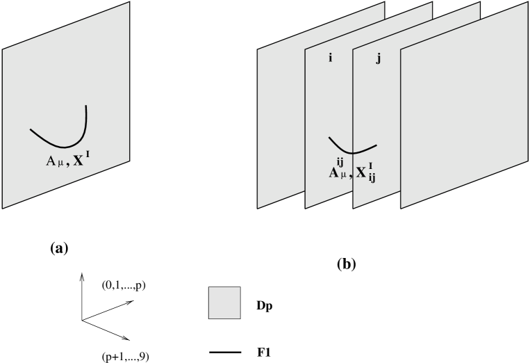
FIG. 1.: Low lying states of fundamental strings with both ends on D-branes describe a $U(1)$ gauge field and $9-p$ scalars living on a single D-brane (a), or a $U(N_{c})$ gauge field and $9-p$ adjoint scalars on a stack of $N_{c}$ D-branes (b).

The $Dp$-brane is charged under a Ramond-Ramond (RR) $(p+1)$-form potential of the type II string. As we saw, in type IIA string theory there are such potentials with even $p$ and, therefore, $Dp$-branes with $p=0,2,4,6,8$. Similarly, in type IIB string theory there are potentials with odd $p$ and $Dp$-branes with $p=-1,1,3,5,7,9$. The $p=-1$ brane is the D-instanton, while the $p=9$ brane is the $D9$-brane that fills the whole $9+1$ dimensional spacetime and together with the orientifold (to be described below) turns a type IIB string into a type I one. The $D7$-brane is the ”magnetic dual” of the D-instanton; the $D8$-brane together with the orientifold turns a type IIA string into a type I’ one.

The tension of a $Dp$-brane is

$$T_{p}={1\over g_{s}l_{s}^{p+1}}$$ (7)

where $l_{s}$ is the fundamental string scale (the tension of the fundamental string is $T=1/l_{s}^{2}$). The $Dp$-brane tension (7) is equal to its RR charge; D-branes are BPS saturated objects preserving half of the thirty two supercharges of type II string theory. More precisely, a $Dp$-brane stretched along the $(x^{1},\cdots,x^{p})$ hyperplane preserves supercharges of the form $\epsilon_{L}Q_{L}+\epsilon_{R}Q_{R}$ with

$$\epsilon_{L}=\Gamma^{0}\Gamma^{1}\cdots\Gamma^{p}\epsilon_{R}$$ (8)

An anti $Dp$-brane carries the opposite RR charge and preserves the other half of the supercharges. Equation (8) can be thought of as arising from the presence in the theory of open strings that end on the branes. In the presence of such open strings the left and right moving supercharges $Q_{L}$, $Q_{R}$ (2,4) are not independent; eq. (8) describes the reflection of right to left movers at the boundary of the worldsheet, which is confined to the brane.

The low energy worldvolume theory on an infinite $Dp$-brane is a $p+1$ dimensional field theory invariant under sixteen supercharges. It describes the dynamics of the ground states of open strings both of whose endpoints lie on the brane (Fig. 1(a)). The massless spectrum includes a $p+1$ dimensional $U(1)$ gauge field $A_{\mu}(x^{\nu})$, $9-p$ scalars $X^{I}(x^{\mu})$ ($I=p+1,\cdots,9$, $\mu=0,\cdots,p$) parametrizing fluctuations of the $Dp$-brane in the transverse directions, and fermions required for SUSY . The low energy dynamics can be obtained by dimensional reduction of $N=1$ SYM with gauge group $G=U(1)$ from $9+1$ to $p+1$ dimensions. The bosonic part of the low energy worldvolume action is

$$S={1\over g_{SYM}^{2}}\int d^{p+1}x\left({1\over 4}F_{\mu\nu}F^{\mu\nu}+{1\over l_{s}^{4}}\partial_{\mu}X^{I}\partial^{\mu}X_{I}\right)$$ (9)

The $U(1)$ gauge coupling on the brane $g_{SYM}$ is given by

$$g_{SYM}^{2}=g_{s}l_{s}^{p-3}$$ (10)

The $g_{s}$ dependence in (7,10) follows from the fact that the kinetic term (9) arises from open string tree level (the disk), while the power of the string length $l_{s}$ is fixed by dimensional analysis.

At high energies, the massless degrees of freedom (9) interact with an infinite tower of “open string” states localized on the brane, and with closed strings in the $9+1$ dimensional bulk of spacetime. To study SYM on the brane one needs to decouple the gauge theory degrees of freedom from gravity and massive string modes. To achieve that one can send $l_{s}\to 0$ holding $g_{SYM}$ fixed. This means (10) $g_{s}\to 0$ for $p<3$, $g_{s}\to\infty$ for $p>3$. For $p=3$ $g_{SYM}$ is independent of $l_{s}$ and the $l_{s}\to 0$ limit describes $N=4$ SYM in $3+1$ dimensions. Note that for $p\leq 3$ the above limit leads to a consistent theory on the brane, whose UV behavior is just that of $p+1$ dimensional SYM. For $p>3$ SYM provides a good description in the infrared, but it must break down at high energies.

Since D-branes are BPS saturated objects, parallel branes do not exert forces on each other. The low energy worldvolume dynamics on a stack of $N_{c}$ nearby parallel $Dp$-branes (Fig. 1(b)) is a SYM theory with gauge group $U(N_{c})$ and sixteen supercharges, arising from ground states of open strings whose endpoints lie on the branes [185, 235]. The scalars $X^{I}$ (9) turn into $N_{c}\times N_{c}$ matrices transforming in the adjoint representation of the $U(N_{c})$ gauge group. The $N_{c}$ photons in the Cartan subalgebra of $U(N_{c})$ and the diagonal components of the matrices $X^{I}$ correspond to open strings both of whose endpoints lie on the same brane. The charged gauge bosons and off-diagonal components of $X^{I}$ correspond to strings whose endpoints lie on different branes. Specifically, the $(i,j)$, $(j,i)$ elements of $X^{I}$, $A_{\mu}$ arise from the two orientations of a fundamental string connecting the $i$’th and $j$’th branes (see Fig. 1(b)).

The generalization of (9) to the case of $N_{c}$ parallel $Dp$-branes is described by dimensional reduction of $N=1$ SYM with gauge group $G=U(N_{c})$ from $9+1$ to $p+1$ dimensions. The bosonic part of the $9+1$ dimensional low energy Lagrangian,

$${\cal L}={1\over 4g_{SYM}^{2}}{\rm Tr}F_{mn}F^{mn};\;\;m,n=0,1,\cdots,9$$ (11)

$$F_{mn}=\partial_{m}A_{n}-\partial_{n}A_{m}-i[A_{m},A_{n}]$$ (12)

gives rise upon dimensional reduction to kinetic terms for the $p+1$ dimensional gauge field $A_{\mu}$ and adjoint scalars $X^{I}$,

$${\cal L}_{\rm kin}={1\over g_{SYM}^{2}}{\rm Tr}\left({1\over 4}F_{\mu\nu}F^{\mu\nu}+{1\over l_{s}^{4}}{\cal D}_{\mu}X^{I}{\cal D}^{\mu}X_{I}\right)$$ (13)

(${\cal D}_{\mu}X^{I}=\partial_{\mu}X^{I}-i[A_{\mu},X^{I}]$; $F_{\mu\nu}=\partial_{[\mu}A_{\nu]}-i[A_{\mu},A_{\nu}]$), and to a potential for the adjoint scalars $X^{I}$,

$$V\sim{1\over l_{s}^{8}g_{SYM}^{2}}\sum_{I,J}{\rm Tr}\;[X^{I},X^{J}]^{2}$$ (14)

Flat directions of the potential (14) corresponding to diagonal $X^{I}$ (up to gauge transformations) parametrize the Coulomb branch of the $U(N_{c})$ gauge theory. The moduli space of vacua is $(R^{9-p})^{N_{c}}/S_{N_{c}}$; it is parametrized by the eigenvalues of $\vec{X}$,

$$\vec{x}_{i}=\langle\vec{X}_{ii}\rangle;\;\;\;i=1\cdots,N_{c}$$ (15)

which label the transverse locations of the $N_{c}$ branes. The permutation group $S_{N_{c}}$ acts on $\vec{x}_{i}$ as the Weyl group of $SU(N_{c})$. For generic positions of the $N_{c}$ branes, the off-diagonal components of $X^{I}$ as well as the charged gauge bosons are massive (and the gauge symmetry is broken, $U(N_{c})\to U(1)^{N_{c}}$). Their masses are read off (13-15):

$$m_{ij}={1\over l_{s}^{2}}|\vec{x}_{i}-\vec{x}_{j}|$$ (16)

Geometrically (16) can be thought of as the minimal energy of a fundamental string stretched between the $i$’th and $j$’th branes (Fig. 1(b)). When $n$ of the $N_{c}$ branes coincide, some of the charged particles become massless (16) and the gauge group is enhanced from $U(1)^{N_{c}}$ to $U(n)\times U(1)^{N_{c}-n}$.

2 Orientifolds

An orientifold $p$-plane ($Op$-plane) is a generalization of a $Z_{2}$ orbifold fixed plane to non-oriented string theories [188, 187]. It can be thought of as the fixed plane under a $Z_{2}$ symmetry which acts on the spacetime coordinates and reverses the orientation of the string. The fixed plane of the $Z_{2}$ transformation 

$$x^{I}(z,\bar{z})\leftrightarrow-x^{I}(\bar{z},z);\;\;I=p+1,\cdots,9$$ (17)

is an $Op$-plane extending in the $(x^{1},\cdots,x^{p})$ directions and time.

Like usual orbifold fixed planes, the orientifold is not dynamical (at least at weak string coupling). It carries charge under the same RR $(p+1)$-form gauge potential, and breaks the same half of the SUSY, as a parallel $Dp$-brane. In the presence of an $Op$-plane, the transverse space $R^{9-p}$ is replaced by $R^{9-p}/Z_{2}$. It is convenient to continue to describe the geometry as $R^{9-p}$, add a $Z_{2}$ image for each object lying outside the fixed plane and implement an appropriate (anti-) symmetrization on the states. Thus D-branes which are outside the orientifold plane acquire mirror images (see Fig. 2). At the fixed plane one can sometimes have a single D-brane which does not have a $Z_{2}$ partner and hence cannot leave the singularity. The RR charge of an $Op$-plane $Q_{Op}$ is equal (up to a sign) to that of $2^{p-4}$ $Dp$-branes (or $2^{p-5}$ pairs of a $Dp$-brane and its mirror). Denoting the RR charge of a $Dp$-plane by $Q_{Dp}$, the orientifold charge is:

$$Q_{Op}=\pm 2\cdot 2^{p-5}Q_{Dp}$$ (18)

(this will be further discussed later). The (anti-) symmetric projection imposed on D-branes by the presence of an orientifold plane leads to changes in their low energy dynamics. On a stack of $N_{c}$ $Dp$-branes parallel to an $Op$-plane one finds a gauge theory with sixteen supercharges and the following rank $[N_{c}/2]$ gauge group  $G$:

• $Q_{Op}=+2\cdot 2^{p-5}Q_{Dp}$, $N_{c}$ even: $G=Sp(N_{c}/2)$.

• $Q_{Op}=-2\cdot 2^{p-5}Q_{Dp}$: $G=SO(N_{c})$.

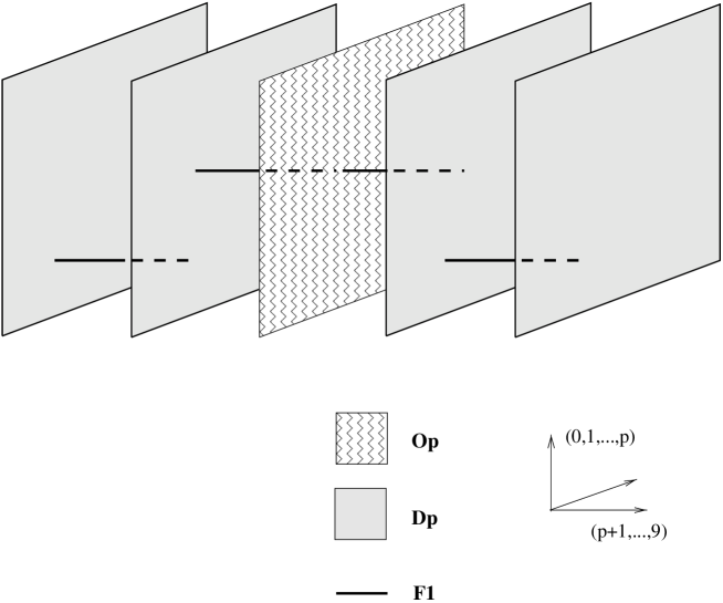
FIG. 2.: An orientifold $p$-plane with two adjacent parallel $Dp$-branes and their mirror images. Fundamental strings stretched between a D-brane and its image are projected out for negative orientifold charge. Others come in mirror pairs.

The light matter consists of the ground states of open strings stretched between different D-branes, giving rise to a gauge field for the group $G$ and $9-p$ scalars $X^{I}$ in the adjoint of $G$. Positive orientifold charge gives rise to a symmetric projection on the $N_{c}\times N_{c}$ matrices $A_{\mu}$, $X^{I}$ and, therefore, a symplectic gauge group ($N_{c}$ must be even in that case; as is clear from (17), for the case of a symmetric projection it is impossible to have a D-brane without an image stuck at the orientifold), while negative orientifold charge leads to an antisymmetric projection and to orthogonal gauge groups.

Geometrically, $(N_{c}^{2}\pm N_{c})/2$ of the $N_{c}^{2}$ oriented strings stretched between the $N_{c}$ $Dp$-branes survive the (anti-) symmetric projection due to the orientifold. The difference of $N_{c}$ between the symmetric and antisymmetric cases corresponds to strings stretching between a $Dp$-brane and its mirror image. These strings transform to themselves under the combined worldsheet and spacetime reflection (17); thus they are projected out in the antisymmetric case, and give $2\times N_{c}/2$ massless modes in the symmetric case.

Since branes can only leave the orientifold plane in pairs, there are $[N_{c}/2]$ “dynamical branes” which are free to move. Their locations in the transverse space $R^{9-p}$ parametrize the Coulomb branch of the theory. The $[N_{c}/2]$ photons in the Cartan subalgebra of $G$ and the scalars parametrizing the Coulomb branch correspond to open strings both of whose endpoints lie on the same brane. When $n$ of the $[N_{c}/2]$ $Dp$-branes coincide outside the orientifold plane the gauge symmetry is enhanced from $U(1)^{[N_{c}/2]}$ to $U(n)\times U(1)^{[N_{c}/2]-n}$. When $m$ of the $N_{c}$ branes coincide with the orientifold plane the gauge group is enhanced to $\left(SO(m)\;{\rm or}\;Sp(m/2)\right)\times U(1)^{[(N_{c}-m)/2]}$.

For high dimensional orientifolds and D-branes the discussion above has to be slightly modified. In particular, for $p\geq 7$ the rank of the gauge group $G$ is bounded since RR flux does not have enough non-compact transverse directions to escape, and therefore the total RR charge must vanish. The case $p=9$ is further special, since there are no transverse directions at all and the reflection (17) acts only on the worldsheet. The requirement that the total RR charge vanish and the orientifold charge $Q_{O9}=-32$ (see (18)) are in this case directly related to the fact that the gauge group of ten dimensional type I string theory is $SO(32)$. The $p$ dependence in (18) will be discussed in section II D.

3 The Solitonic Fivebrane

The solitonic fivebrane [59] which exists in weakly coupled type II and heterotic string theory, is a BPS saturated object which, like the Dirichlet brane, preserves half of the supersymmetry of the theory and has tension

$$T_{NS}={1\over g_{s}^{2}l_{s}^{6}}$$ (19)

It couples magnetically to the NS-NS sector $B_{\mu\nu}$ field and can thus be thought of as a magnetic dual of the fundamental type II or heterotic string. Since its tension is proportional to $1/g_{s}^{2}$ it provides a non-trivial background for a fundamental string in leading order in $g_{s}$ (i.e. on the sphere). A fundamental string propagating in the background of $k$ parallel NS fivebranes located at transverse positions $\vec{x}_{i}$ is described by a conformal field theory (CFT) with non-trivial $G_{IJ}$, $B_{IJ}$, $\Phi$ (metric, antisymmetric tensor and dilaton) given by:

$$e^{2(\Phi-\Phi_{0})}=1+\sum_{j=1}^{k}{l_{s}^{2}\over|\vec{x}-\vec{x}_{j}|^{2}}$$ (20)

$$G_{IJ}=e^{2(\Phi-\Phi_{0})}\delta_{IJ};\;G_{\mu\nu}=\eta_{\mu\nu}$$ (21)

$$H_{IJK}=-\epsilon_{IJKM}\partial^{M}\Phi$$ (22)

$I,J,K,M$ label the four directions transverse to the fivebrane; $\mu,\nu$ label the $5+1$ longitudinal directions. $H$ is the field strength of $B$; $\Phi_{0}$ is the value of the dilaton at infinity, related to the string coupling at infinity $g_{s}=\exp\Phi_{0}$. As is clear from (22), the effective string coupling $\exp\Phi$ depends on the distance from the fivebrane, diverging at the core.

An NS fivebrane stretched in the $(x^{1},\cdots,x^{5})$ hyperplane preserves supercharges of the form $\epsilon_{L}Q_{L}+\epsilon_{R}Q_{R}$, where for the type IIA fivebrane

$$\epsilon_{L}= \Gamma^{0}\Gamma^{1}\Gamma^{2}\Gamma^{3}\Gamma^{4}\Gamma^{5}\epsilon_{L}$$ (23)

$$\epsilon_{R}= \Gamma^{0}\Gamma^{1}\Gamma^{2}\Gamma^{3}\Gamma^{4}\Gamma^{5}\epsilon_{R}$$ (24)

while for the type IIB fivebrane

$$\epsilon_{L}= \Gamma^{0}\Gamma^{1}\Gamma^{2}\Gamma^{3}\Gamma^{4}\Gamma^{5}\epsilon_{L}$$ (25)

$$\epsilon_{R}= -\Gamma^{0}\Gamma^{1}\Gamma^{2}\Gamma^{3}\Gamma^{4}\Gamma^{5}\epsilon_{R}$$ (26)

Thus, the non-chiral type IIA string theory gives rise to a chiral fivebrane worldvolume theory with (2,0) SUSY in six dimensions, while the chiral type IIB theory gives rise to a non-chiral fivebrane with (1,1) worldvolume SUSY. Equations (24,26) can be established by a direct analysis of the supercharges preserved by the background (22). As we will see later, string duality relates them to the supercharges preserved by D-branes (8), and both have a natural origin in eleven dimensions.

The light fields on the worldvolume of a single type IIA NS fivebrane correspond to a tensor multiplet of six dimensional $(2,0)$ SUSY, consisting of a self-dual $B_{\mu\nu}$ field and five scalars (and the fermions needed for SUSY). On a single type IIB fivebrane one finds a vectormultiplet, i.e., a six dimensional gauge field and four scalars ($+$ fermions).

The four scalars in the vectormultiplet on the type IIB fivebrane, as well as four of the five scalars in the tensor multiplet on the type IIA fivebrane, describe fluctuations of the NS-brane in the transverse directions. The fifth scalar on a type IIA fivebrane lives on a circle of radius $l_{s}$ and provides a hint of a hidden eleventh dimension of quantum type IIA string theory (more on this below).

The gauge coupling of the vector field on the type IIB fivebrane is 

$$g_{SYM}^{2}=l_{s}^{2}$$ (27)

Since NS-branes are BPS saturated objects, parallel branes do not exert forces on each other. The low energy worldvolume dynamics on a stack of $k$ parallel type IIB $NS5$-branes is a $5+1$ dimensional (1,1) $U(k)$ SYM theory (with sixteen supercharges), arising from the ground states of D-strings stretched between different NS-branes. It is described by (13, 14, 27) with $p=5$. As for D-branes, the four scalars in the vector multiplet are promoted to $k\times k$ matrices, whose diagonal components parametrize the Coulomb branch of the theory, $R^{4k}/S_{k}$.

The low energy theory describing a stack of $k$ parallel type IIA $NS5$-branes is more exotic. It can be thought of as a non-abelian generalization of the free theory of a tensor multiplet on a single $NS5$-brane, and gives rise to a non-trivial field theory with $(2,0)$ SUSY in $5+1$ dimensions [234, 218, 206]. It contains string-like low energy excitations corresponding to Dirichlet membranes stretched between the different $NS5$-branes. These strings are charged under the self-dual $B_{\mu\nu}$ fields on the corresponding fivebranes and are light when the fivebranes are close to each other. The Coulomb branch of the (2,0) theory, $(R^{4}\times S^{1})^{k}/S_{k}$, is parametrized by the expectation values of the diagonal components of the five scalars in the tensor multiplet. At the origin of the Coulomb branch, the $(2,0)$ field theory corresponds to a non-trivial superconformal field theory.

In the limit $g_{s}\to 0$ the dynamics of the full type II string theory simplifies and, in particular, all the modes in the bulk of spacetime (including gravity) decouple. The dynamics of a type II string vacuum with $k$ NS fivebranes remains non-trivial in the limit; in the type IIA case it is described at low energies by the (2,0) field theory described above. The theory of $k$ type IIB fivebranes has (1,1) SUSY and reduces at low energies to the (infrared free) $U(k)$ SYM theory; at finite energies it is interacting. Providing a useful description of the fivebrane theory and, in particular, of the low energy $(2,0)$ field theory of the IIA fivebranes remains a major challenge as of this writing.

4 The Kaluza-Klein Monopole

Compactified type II string theory has additional solitonic objects. One that will be particularly useful later is the Kaluza-Klein (KK) monopole, which is a fivebrane in ten dimensions [223, 84]. It is obtained when one of the ten directions, call it $\rho$, is compactified on a circle of radius $R$. The ten dimensional graviton gives rise in nine dimensions to a gauge field $A_{a}=G_{a,\rho}$ ($a=0,\cdots,8$). The KK monopole carries magnetic charge $R/l_{s}$ under this gauge field. Like the monopole of $3+1$ dimensional gauge theory it is localized in three additional directions $\vec{r}$ and is extended in the remaining five.

The tension of the KK fivebrane is

$$T_{KK}={R^{2}\over g_{s}^{2}l_{s}^{8}}$$ (28)

The factor of $1/g_{s}^{2}$ is due to the fact that, like the NS fivebrane, the KK fivebrane “gets its tension” from the sphere (i.e. it is a “conventional soliton”). The other factors in (28) are the square of the magnetic charge and a $1/l_{s}^{6}$ due to the fact that this is a fivebrane.

A fundamental string in the background of $k$ parallel KK monopoles located at transverse positions ${\vec{r}}_{i}$ is described by a CFT with the multi Taub-NUT metric ($B$=$\Phi$=const):

$$ds^{2}=dx^{\mu}dx_{\mu}+ds^{2}_{\bot}$$ (29)

$$ds^{2}_{\bot}=Ud{\vec{r}}^{2}+U^{-1}(d\rho+{\vec{\omega}}\cdot d{\vec{r}})^{2}$$ (30)

where $x^{\mu}$ label the $1+5$ longitudinal directions,

$$U=1+\sum_{j=1}^{k}{R\over 2|{\vec{r}}-{\vec{r}}_{j}|}$$ (31)

and $\vec{w}$ is the multi Dirac monopole vector potential which satisfies

$${\vec{\nabla}}\times{\vec{\omega}}={\vec{\nabla}}U$$ (32)

In the limit $R\to\infty$ this background becomes an ALE space with $A_{k-1}$ singularity. On the other hand, in the $R\to 0$ limit the multi Taub-NUT background (30-32) is T-dual (in the $\rho$ direction and in an appropriate sense [119]) to the multi NS fivebrane solution (22) (more on T-duality later).

C M-Theory Interpretation

All the different ten dimensional string theories can be thought of as asymptotic expansions around different vacua of a single quantum theory. This theory, known as “M-theory,” is in fact $1+10$ dimensional at almost all points in its moduli space of vacua (for a review see, for example [197, 223] and references therein).

In the flat $1+10$ dimensional Minkowski vacuum the theory reduces at low energies to eleven dimensional supergravity. There is no adjustable dimensionless coupling; the only parameter in the theory is the eleven dimensional Planck scale $l_{p}$. Physics is weakly coupled and well approximated by semiclassical supergravity for length scales much larger than $l_{p}$. It is strongly coupled at scales smaller than $l_{p}$. The spectrum includes a three-form potential $A_{MNP}$ ($M,N,P=0,1,\cdots,10$) whose electric and magnetic charges appear as central extensions in the eleven dimensional superalgebra,

$$\{Q_{\alpha},Q_{\beta}\}=(\Gamma^{M}C)_{\alpha\beta}P_{M}+{1\over 2}(\Gamma_{MN}C)_{\alpha\beta}Z^{MN}+{1\over 5!}(\Gamma_{MNPQR}C)_{\alpha\beta}Y^{MNPQR}$$ (33)

where $\Gamma_{MN\cdots}$ are antisymmetrized products of the $32\times 32$ Dirac matrices in eleven dimensions, $C$ is the (real, antisymmetric) charge conjugation matrix, $Z^{MN}$ is the electric charge corresponding to $A_{MNP}$, and $Y^{MNPQR}$ is the corresponding magnetic charge.

A solitonic M-theory membrane/fivebrane ($M2/M5$) carries electric/magnetic charge $Z/Y$ and breaks half of the thirty two supercharges $Q$ (33). An $Mp$-brane ($p=2,5$) stretched in the $(x^{1},\cdots,x^{p})$ directions preserves the supercharges $\epsilon Q$ with

$$\Gamma^{0}\Gamma^{1}\cdots\Gamma^{p}\epsilon=\epsilon$$ (34)

Its tension is fixed by SUSY to be $T_{p}=1/l_{p}^{p+1}$. Large charge branes can be reliably described by eleven dimensional supergravity. The metric around a collection of $k$ $Mp$-branes located at $\vec{r}=\vec{r}_{j}$ ($j=1,\cdots,k$; $\vec{r},\vec{r}_{j}$ are $10-p$ dimensional vectors) is given by:

$$ds^{2}=U^{-1/3}dx^{\mu}dx_{\mu}+U^{2/3}d\vec{r}\cdot d\vec{r}$$ (35)

where $x^{\mu}$ are the $p+1$ directions along the brane, and

$$U=1+\sum_{j=1}^{k}{l_{p}^{8-p}\over|\vec{r}-\vec{r}_{j}|^{8-p}}$$ (36)

and there is also a three index tensor field which we do not specify.

The ten dimensional type IIA vacuum with string coupling $g_{s}$ can be thought of as a compactification of M-theory on $R^{1,9}\times S^{1}$. Denoting the $1+9$ dimensional Minkowski space of type IIA string theory by $(x^{0},x^{1},\cdots,x^{9})$, and the compact direction by $x^{10}$, the compactification radius $R_{10}$ and $l_{p}$ are related to the type IIA parameters $g_{s}$, $l_{s}$ by:

$${R_{10}\over l_{p}^{3}}={1\over l_{s}^{2}}$$ (37)

$$R_{10}=g_{s}l_{s}$$ (38)

Thus, the strong coupling limit of type IIA string theory $g_{s}\to\infty$ (or equivalently $R_{10}/l_{p}\to\infty$) is described by the $1+10$ dimensional Minkowski vacuum of M-theory.

Type IIA branes have a natural interpretation in M-theory:

• A fundamental IIA string stretched (say) along $x^{1}$ can be thought of as an $M2$-brane wrapped around $x^{10}$ and $x^{1}$. It is charged under the gauge field $B_{\mu 1}=A_{10\mu 1}$. Equation (37) is the relation between the wrapped membrane and string tensions.

• The $D0$-brane corresponds to a Kaluza-Klein (KK) mode of the graviton carrying momentum $1/R_{10}$ along the compact direction. It is electrically charged under $G_{\mu,10}$. Equation (38) relates the masses of the KK mode of the graviton and $D0$-brane.

• The $D2$-brane corresponds to a “transverse” $M2$-brane, unwrapped around $x^{10}$. It is charged under $A_{\mu\nu\lambda}$. The tension of the $M2$-brane $1/l_{p}^{3}$ reduces to (7) using the relation

  $$l_{p}^{3}=l_{s}^{3}g_{s}$$ (39)

  which follows from (37, 38).

• The $D4$-brane corresponds to an $M5$-brane wrapped around $x^{10}$. It is charged under the five-form gauge field $\tilde{A}_{10\mu_{1}\mu_{2}\cdots\mu_{5}}$ dual to $A$ $(d\tilde{A}=*dA)$. Its tension (7) is equal to $R_{10}/l_{p}^{6}$ (39).

• The $NS5$-brane corresponds to a transverse $M5$-brane, and is thus charged under $\tilde{A}_{\mu_{1}\cdots\mu_{6}}$. Its tension (19) is equal to $1/l_{p}^{6}$.

• The $D6$-brane is a KK monopole. It is magnetically charged under the gauge field $A_{\mu}=G_{\mu 10}$.

• The $D8$-brane is a mysterious object in M-theory whose tension is known to be $R_{10}^{3}/l_{p}^{12}$ [88].

All this can be summarized by decomposing the representations of $SO(10,1)$ appearing in (33) into representations of $SO(9,1)$ and rewriting the supersymmetry algebra (33) as

$$\{Q_{\alpha},Q_{\beta}\} =(C\Gamma^{\mu})_{\alpha\beta}P_{\mu}+(C\Gamma^{10})_{\alpha\beta}P_{10}+(C\Gamma^{\mu}\Gamma^{10})_{\alpha\beta}Z_{\mu}+{1\over 2}(C\Gamma^{\mu\nu})_{\alpha\beta}Z_{\mu\nu}$$ (40)

$$+{1\over 4!}(C\Gamma^{\mu\nu\rho\sigma}\Gamma^{10})_{\alpha\beta}Y_{\mu\nu\rho\sigma}+{1\over 5!}(C\Gamma^{\mu\nu\rho\sigma\lambda})_{\alpha\beta}Y_{\mu\nu\rho\sigma\lambda}$$ (41)

where $9+1$ dimensional vector indices are denoted by $\mu,\nu,\rho,\sigma,\cdots$. The momentum in the eleventh direction $P_{10}$ is reinterpreted in ten dimensions as zero-brane charge; the spatial components of $Z_{\mu}$ are carried by “fundamental” IIA strings. Similarly, $Z_{\mu\nu}$ is the $D2$-brane charge, $Y_{\mu\nu\rho\sigma}$ is the $D4$-brane charge, and $Y_{\mu\nu\rho\sigma\lambda}$ is carried by $NS5$-branes. The different preserved supersymmetries (8, 24) combine in eleven dimensions into the single relation (34). Note that (41) includes central charges for $p$-branes with $p\leq 5$. Higher branes (e.g. the $D6$-brane) are inherently tied to compactification; therefore the corresponding central charges have to be added to (41) by hand.

We mentioned above that the scalar $X^{10}$ describing fluctuations of the IIA fivebrane in $x^{10}$ lives on a circle of radius $l_{s}$. From the point of view of compactified M-theory it is clear that the scalar field $X^{10}$ lives on a circle of radius proportional to $R_{10}$; the proportionality constant is determined for a canonically normalized $X^{10}$ by dimensional analysis to be $1/l_{p}^{3}$ as scalars in $5+1$ dimensions have scaling dimension two. Using (37) we arrive at the conclusion that the radius of (canonically normalized) $X^{10}$ is $R_{10}/l_{p}^{3}=1/l_{s}^{2}$. In the normalization used in (9), with $g_{SYM}=l_{s}$ (27), $X$ has dimensions of length and lives on a circle of radius $l_{s}$.

The metric around an $M5$-brane transverse to $x^{10}$ (35, 36) goes over to that around the $NS5$-brane (22) as $R_{10}\to 0$. To see that, describe an $M5$-brane at $x^{10}=0$ on the circle as an infinite stack of parallel fivebranes located at $x^{10}=nR_{10}$ ($n=0,\pm 1,\pm 2,\cdots$). The harmonic function $U$ (36) is

$$U=1+\sum_{n}\left[{l_{p}^{2}\over|\vec{x}|^{2}+(nR_{10})^{2}}\right]^{3\over 2}$$ (42)

As $R_{10}\to 0$ one can replace the sum by an integral and (42) approaches (using (37))

$$U\simeq 1+l_{s}^{2}/|\vec{x}|^{2}$$ (43)

The component of the metric $G_{10,10}=U^{2/3}$ (35) is related to the ten dimensional dilaton via $G_{10,10}\equiv\exp(2\gamma)=\exp(4\phi/3)$. The string metric ${\cal G}$ is related to the eleven dimensional metric $G$ by a rescaling ${\cal G}=G\exp\gamma$. Performing the rescaling leads to the ten dimensional form (22).

Ten dimensional type IIB string theory has a complex coupling

$$\tau=a+{i\over g_{s}},$$ (44)

where $a$ is the expectation value of the massless RR scalar. In the eleven dimensional interpretation, the ten dimensional type IIB vacuum corresponds to M-theory compactified on a two-torus of complex structure $\tau$ and vanishing area. Naively, the theory appears to be $1+8$ dimensional in this limit, but in fact as the size of the torus goes to zero, the wrapping modes of the $M2$-brane become light and give rise to another non-compact direction which we will label by $x^{B}$.

M-theory on a finite two-torus corresponds to compactifying $x^{B}$ on a circle of radius $R_{B}$. In the special case $a=0$, the M-theory two-torus is rectangular with sides $R_{9},R_{10}$. The mapping of the M-theory parameters $(R_{9},R_{10},l_{p})$ to the type IIB ones $(R_{B},g_{s},l_{s})$ is:

$${R_{10}\over l_{p}^{3}}={1\over l_{s}^{2}}$$ (45)

$${R_{9}\over l_{p}^{3}}={1\over g_{s}l_{s}^{2}}$$ (46)

$${R_{9}R_{10}\over l_{p}^{3}}={1\over R_{B}}$$ (47)

One way to establish (45-47) is to reinterpret the different type IIB branes in M-theory:

• A fundamental IIB string can be thought of as an $M2$-brane wrapped around $x^{10}$. Equation (45) is the relation between the membrane and string tensions.

• A $D1$-brane (D-string) that is not wrapped around $x^{B}$ corresponds to an $M2$-brane wrapped around $x^{9}$. Equation (46) is the relation between the membrane and D-string tensions. A D-string wrapped around $x^{B}$ corresponds to a KK mode of the eleven dimensional supergraviton carrying momentum in the $x^{10}$ direction. E.g., using (45) and the relation

  $${1\over l_{p}^{3}}={R_{B}\over g_{s}l_{s}^{4}}$$ (48)

  which follows from (45-47), the masses agree: $1/R_{10}=R_{B}/g_{s}l_{s}^{2}$.

• A KK mode of the supergraviton carrying momentum in the $x^{B}$ direction in type IIB string theory corresponds to an $M2$-brane wrapped around $(x^{9},x^{10})$; eq. (47) relates the masses of the two.

• A $D3$-brane unwrapped around $x^{B}$ corresponds to an $M5$-brane wrapped on $(x^{9},x^{10})$. The tension of the wrapped $M5$-brane $R_{9}R_{10}/l_{p}^{6}$ reduces to (7) using (45, 46). A $D3$-brane wrapped around $x^{B}$ corresponds to an $M2$-brane.

• A $D5$-brane wrapped around $x^{B}$ corresponds to an $M5$-brane wrapped around $x^{10}$. The tension of the wrapped $M5$-brane $R_{10}/l_{p}^{6}$ reduces to $R_{B}/g_{s}l_{s}^{6}$ using (48). A $D5$-brane unwrapped around $x^{B}$ corresponds to a KK monopole charged under the gauge field $G_{\mu,10}$ and wrapped around $x^{9}$.

• The $NS5$-brane wrapped around $x^{B}$ corresponds to an $M5$-brane wrapped on $x^{9}$. Its tension $R_{B}/g_{s}^{2}l_{s}^{6}$ is equal to that of the wrapped $M5$-brane $R_{9}/l_{p}^{6}$. An NS fivebrane unwrapped around $x^{B}$ corresponds to a KK monopole charged under the gauge field $G_{\mu,9}$ and wrapped around $x^{10}$.

• The $D7$-brane wrapped around $x^{B}$ corresponds to a KK monopole charged under $G_{\mu,10}$. A $D7$-brane unwrapped around $x^{B}$ is related to the M-theory eightbrane which reduces to the $D8$-brane of IIA string theory.

Orientifolds correspond in M-theory to fixed points of $Z_{2}$ transformations acting both on space and on the supergravity fields.

D Duality Properties

String (or M-) theory has a large moduli space of vacua ${\cal M}$ parametrized by the size and shape of the compact manifold and the string coupling (as well as the values of other background fields). At generic points in ${\cal M}$ the theory is eleven dimensional and inherently quantum mechanical while at certain degenerations it has different weakly coupled string expansions.

The space of vacua ${\cal M}$ is a non-trivial manifold; in particular, it has an interesting global structure. Some apparently distinct vacua are identified by the action of a discrete group known as “U-duality” [135]. Under this identification different states of the theory are often mapped into each other; an example is the BPS branes discussed above. What looks like a D-brane in one description may appear to be an NS-brane in another, and may even correspond to an object of different dimension.

An important subgroup of U-duality is T-duality which takes a weakly coupled vacuum to another weakly coupled vacuum and is, therefore, manifest in string perturbation theory (for a review see [111] and references therein). Consider type IIA string theory in $1+8$ non-compact dimensions with the $i$’th coordinate $x^{i}$ living on a circle of radius $R_{i}$. At large $R_{i}$ the theory becomes $1+9$ dimensional IIA string theory while at small $R_{i}$ it naively becomes $1+8$ dimensional. However, winding type IIA strings with energy $nR_{i}/l_{s}^{2}$ become light in the limit, producing a continuous Kaluza-Klein spectrum and thus the theory becomes ten dimensional again.

From the discussion of the previous section it is clear what the new $1+9$ dimensional theory is. Weakly coupled type IIA string theory on a small circle $R_{i}\to 0$ corresponds to M-theory on a vanishing two-torus, which we saw before is just type IIB string theory. How do different states in IIA string theory map to their IIB counterparts?

The wrapped IIA string is a wrapped $M2$-brane (see (37) and subsequent discussion); the modes becoming light in the $R_{i}\to 0$ limit correspond to membranes wrapped $n$ times around the shrinking two-torus labeled by $(x^{i},x^{10})$. Comparing their energy $nR_{i}R_{10}/l_{p}^{3}$ to (47) and using (37-46) we see that the IIB string one finds lives on a circle of radius

$$R^{(B)}_{i}={l_{s}^{2}\over R^{(A)}_{i}}$$ (49)

and has string coupling

$$g_{s}^{(B)}=g_{s}^{(A)}l_{s}/R^{(A)}_{i}$$ (50)

We will refer to the transformation (49, 50) as $T_{i}$ (T-duality in the $i$’th direction).

The different branes of type IIA string theory transform as follows under $T_{i}$:

• As we just saw, a fundamental IIA string wound $n$ times around $x^{i}$ transforms into a fundamental IIB string carrying momentum $n/R^{(B)}_{i}$. An unwound fundamental IIA string carrying momentum $m/R^{(A)}_{i}$ transforms under $T_{i}$ to a fundamental IIB string wound $m$ times around the $i$’th direction.

• A $D0$-brane corresponds in M-theory to a KK graviton carrying momentum $1/R_{10}$. As we saw earlier, in type IIB language this is a D-string wrapped around the $i$’th direction.

• A $D2$-brane wrapped around $x^{i}$ corresponds in M-theory to a transverse $M2$-brane wrapped around $x^{i}$. We saw earlier that in type IIB language this is a D-string unwrapped around $x^{i}$. Similarly, a $D2$-brane unwrapped around $x^{i}$ was seen to correspond to an unwrapped $M2$-brane and was interpreted in IIB language as a $D3$-brane wrapped around $x^{i}$.

• At this point the pattern for Dirichlet branes should be clear. A IIA Dirichlet $p$ brane wrapped around $x^{i}$ is transformed under $T_{i}$ to an unwrapped IIB Dirichlet $p-1$ brane, while an unwrapped IIA Dirichlet $p$ brane is transformed to a Dirichlet $p+1$ brane wrapped around $x^{i}$:

  $$T_{i}:\;\text{{\hbox{Dp}}\ wrapped on {\hbox{x^i}}}\longleftrightarrow\text{{\hbox{D(p-1)}} at a point on {\hbox{x^i}}}$$ (51)

• Orientifold planes transform under $T_{i}$ in the same way as D-branes (51).

• A wrapped IIA NS fivebrane transforms under $T_{i}$ to a wrapped IIB NS fivebrane. An unwrapped IIA NS fivebrane transforms into the KK monopole carrying magnetic charge under $G_{\mu,i}$:

  $$T_{i}:\left\{\begin{array}[]{ll}\mbox{IIA $NS5$ wrapped on $x^{i}$}&\longleftrightarrow\mbox{IIB $NS5$ wrapped on $x^{i}$}\\ \mbox{$NS5$ at a point on $x^{i}$}&\longleftrightarrow\mbox{KK monopole charged under $G_{\mu,i}$}\end{array}\right.$$ (52)

As a check, the tensions of the various (wrapped and unwrapped) Dirichlet and solitonic branes (7, 19, 28) transform under (49, 50) consistently with the above discussion.

The generalization to T-duality in more than one direction $T_{i_{1},i_{2},\cdots,i_{n}}\equiv T_{i_{1}}T_{i_{2}}\cdots T_{i_{n}}$ is straightforward:

$$T_{i_{1},i_{2},\cdots,i_{n}}:\;(R_{i_{1}},R_{i_{2}},\cdots,R_{i_{n}})\longleftrightarrow ({l_{s}^{2}\over R_{i_{1}}},{l_{s}^{2}\over R_{i_{2}}},\cdots,{l_{s}^{2}\over R_{i_{n}}})$$ (53)

$$g_{s}\longleftrightarrow \;g_{s}\prod_{\alpha=1}^{n}{l_{s}\over R_{i_{\alpha}}};\;l_{s}\longleftrightarrow l_{s}$$ (54)

For even $n$ it takes type IIA(B) to itself, while for odd $n$ it exchanges the two.

The discussion above can be used to determine the charge of the $Op$ plane given in (18). Starting with the type I theory on $T^{n}$, which contains a single $O9$-plane and thirty two $D9$-branes wrapped around the $T^{n}$, and performing T-duality, $T_{i_{1},i_{2},\cdots,i_{n}}$, we find a vacuum with $2^{n}$ orientifold $p$-planes, $p=9-n$, one at each fixed point on $T^{n}/Z_{2}$, as well as thirty two $Dp$-branes. The total RR $(p+1)$-form charge of the configuration is zero, which leads to (18).

Another interesting subgroup of U-duality is S-duality of type IIB string theory in $9+1$ dimensions [196], an $SL(2,Z)$ symmetry that acts by fractional linear transformations with integer coefficients on $\tau$ (44). In the M-theory interpretation of IIB string theory, this $SL(2,Z)$ is the modular group acting on the complex structure of the two-torus (whose size goes to zero in the ten dimensional limit). (For a review see [197] and references therein). We will focus on a $Z_{2}$ transformation $S\in SL(2,Z)$ which acts as $\tau\to-1/\tau$; we will furthermore restrict to the case of vanishing RR scalar $a$ (namely a rectangular M-theory two-torus), in which case it acts on the coupling (44) as strong-weak coupling duality: $g_{s}\to 1/g_{s}$. In the M-theory interpretation of IIB string theory discussed in (45-47) $S$ acts geometrically by interchanging $R_{9}\leftrightarrow R_{10}$. Equations (45, 46) imply that the type IIB parameters $g_{s},l_{s}$ transform as:

$$S:\;g_{s}\longleftrightarrow{1\over g_{s}};\;\;l_{s}^{2}\longleftrightarrow l_{s}^{2}g_{s}$$ (55)

Another way to arrive at (55) is to require that as the string coupling is inverted, the ten dimensional Planck length $l_{10}^{4}=g_{s}l_{s}^{4}$ remains fixed. From the discussion following eq. (47) it is clear that the different IIB branes transform under $S$ as follows:

• The fundamental string is interchanged with the D-string.

• The $D3$-brane is invariant.

• The $NS5$-brane is interchanged with the $D5$-brane.

• The $D7$-brane transforms into a different sevenbrane.

As a check, the tensions of the various branes (7, 19) transform under (55) consistently with the above discussion. The transformations of orientifold planes under $S$ are more intricate and will be discussed in the context of particular applications below.

The worldsheet dynamics on both the fundamental string and D-string is that of a critical IIB string. At weak string coupling the tension of the fundamental string is much smaller than that of the D-string, and we can think of the former as “fundamental” and of the latter as a heavy soliton. At strong coupling, the D-string is the lighter object and it should be used as the basis for string perturbation theory. Since a IIB string in its ground state preserves half of the SUSY, it can be followed from weak to strong coupling, and the above picture is indeed reliable.

Under the full $SL(2,Z)$ S-duality group, the two different kinds of strings are members of a multiplet of $(p,q)$ strings, with the fundamental string corresponding to $(p,q)=(1,0)$ and the D-string corresponding to $(p,q)=(0,1)$. $p$ measures the charge carried by the string under the NS-NS $B_{\mu\nu}$ field while $q$ measures the charge under the RR $B_{\mu\nu}$ field. In M-theory the $(p,q)$ string corresponds to a membrane wrapped $p$ times around $x^{10}$ and $q$ times around $x^{9}$; it is stable when $p,q$ are relatively prime. A similar discussion applies to fivebranes that carry magnetic charges under the two $B_{\mu\nu}$ fields and thus form a multiplet of $(p,q)$ fivebranes. There are also $(p,q)$ sevenbranes which carry magnetic charge under the complex dilaton $\tau$.

In M-theory compactified on $T^{d}$, the $SL(2,Z)$ S-dualities corresponding to different $T^{2}\subset T^{d}$ are subgroups of the geometrical $SL(d,Z)$ symmetry group of $T^{d}$. Together with T-duality (54) they generate the U-duality group $E_{d(d)}(Z)$ of type II strings on $T^{d-1}$ [88].

E Webs Of Branes

So far we discussed brane configurations which preserve sixteen supercharges. In this section we will describe some configurations with lower supersymmetry.

We saw before that a stack of parallel D or NS-branes preserves $1/2$ of the SUSY given by (8) or (24, 26), respectively. To find the SUSY preserved by a web of differently oriented D and/or NS-branes one needs to impose all the corresponding conditions  on the spinors $\epsilon$. The worldvolume dynamics on such a web of branes is typically rather rich. We will next consider it in a few examples.

1 The $Dp$ – $D(p+4)$ System

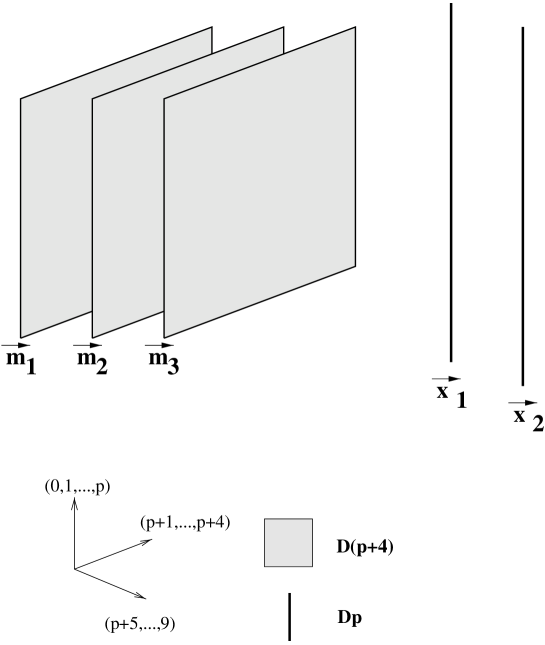
FIG. 3.: The $Dp$ - $D(p+4)$ system consisting of a stack of $N_{c}$ $Dp$-branes parallel to $N_{f}$ $D(p+4)$-branes. Locations in the transverse space $(x^{p+5},\cdots,x^{9})$ are labeled by $\vec{x}_{a}$, $\vec{m}_{i}$, respectively.

Consider a stack of $N_{c}$ $Dp$-branes stretched in the $(x^{1},\cdots,x^{p})$ hyperplane “parallel” to a stack of $N_{f}$ $D(p+4)$-branes stretched in $(x^{1},\cdots,x^{p+4})$ depicted in Figure 3. Each stack preserves $1/2$ of the SUSY and together they preserve $1/2\times 1/2=1/4$ of the thirty two supercharges of type II string theory. The preserved supercharges are those that satisfy (8)

$$\epsilon_{L}=\Gamma^{0}\Gamma^{1}\cdots\Gamma^{p}\epsilon_{R}=\Gamma^{0}\Gamma^{1}\cdots\Gamma^{p+4}\epsilon_{R}$$ (56)

The second equality in (56) is a constraint on $\epsilon_{R}$, $\epsilon_{R}=\Gamma\epsilon_{R}$ with $\Gamma=\Gamma^{p+1}\Gamma^{p+2}\Gamma^{p+3}\Gamma^{p+4}$. The matrix $\Gamma$ squares to the identity matrix, and is traceless. Thus, half of its sixteen eigenvalues are $+1$ and half are $-1$. The constraint on $\epsilon_{R}$, $\Gamma=1$, preserves eight of the sixteen components of $\epsilon_{R}$. Given $\epsilon_{R}$, the first equality in (56) fixes $\epsilon_{L}$. Thus the total number of independent supercharges preserved by the configuration is eight.

The light degrees of freedom on each stack of branes were discussed before. On the $N_{c}$ $Dp$-branes there is a $p+1$ dimensional $U(N_{c})$ gauge theory coupled to $9-p$ adjoint scalars and some fermions. The adjoint scalars naturally split into $5-p$ fields corresponding to fluctuations of the $Dp$-branes transverse to the $(p+4)$-branes which together with the gauge field form the vectormultiplet of a theory with eight supercharges, and the remaining four fields, which form an adjoint hypermultiplet.

A similar theory with $N_{c}\to N_{f}$ and $p\to p+4$ lives on the $D(p+4)$-branes. Each of the two theories has sixteen supercharges. The SUSY of the full theory is broken down to eight supercharges by additional matter corresponding to strings stretched between the two stacks of branes. From the point of view of the $Dp$-brane this matter corresponds to $N_{f}$ flavors in the fundamental representation of $U(N_{c})$. From the point of view of the $D(p+4)$-brane, they are $N_{c}$ pointlike (in the transverse directions) defects in the fundamental of $U(N_{f})$. When the $Dp$-branes are inside the $D(p+4)$-branes, they can be thought of as small instantons [77].

It is important to emphasize that for an observer that lives on the $Dp$-brane, the degrees of freedom on the $D(p+4)$-brane are non-dynamical background fields (at least in infinite volume). For example, the effective gauge coupling in $p+1$ dimensions $g_{p+1}$ of the $U(N_{f})$ gauge field on the $D(p+4)$-brane is given by

$${1\over g_{p+1}^{2}}={V_{p+1,\cdots,p+4}\over g_{p+5}^{2}}$$ (57)

where $g_{p+5}$ is the $U(N_{f})$ gauge coupling in $p+5$ dimensions and $V_{p+1,\cdots,p+4}$ is the volume of the $D(p+4)$-brane worldvolume transverse to the $Dp$-brane. When this volume is infinite, the kinetic energy of $U(N_{f})$ excitations is infinite as well and they are frozen at their classical values. The same is true for other excitations on the $D(p+4)$-brane. Thus, from the point of view of the $Dp$-brane, the $U(N_{f})$ gauge symmetry of the $D(p+4)$-brane is a global symmetry and the only dynamical fields that appear due to the presence of the $D(p+4)$-brane are the $N_{f}$ flavors corresponding to strings stretched between the $Dp$ and $D(p+4)$-branes; these modes are localized at the $Dp$-brane.

The relative locations in space of the various branes correspond to moduli and couplings in the $Dp$-brane worldvolume theory. Locations of the “heavy” $D(p+4)$-branes correspond to couplings while locations of the “light” $Dp$-branes are moduli:

• The locations of the $D(p+4)$-branes in the transverse space $(x^{p+5},\cdots,x^{9})$ $\vec{m}_{i}$ $(i=1,\cdots,N_{f})$ correspond to masses for the $N_{f}$ fundamentals.

• The locations of the $Dp$-branes in $(x^{p+5},\cdots,x^{9})$ $\vec{x}_{a}$ $(a=1,\cdots,N_{c})$ correspond to expectation values of fields $\vec{X}$ in the adjoint of $U(N_{c})$ and parametrize the Coulomb branch of the $U(N_{c})$ gauge theory, as in (15).

• The locations of the $Dp$-branes parallel to the $D(p+4)$-branes (in the $(x^{p+1},\cdots,x^{p+4})$ directions) correspond to expectation values of an adjoint hypermultiplet of $U(N_{c})$.

One can think of the $Dp$-branes as probing the geometry near the $D(p+4)$-brane. For example, the metric on the Coulomb branch of the $U(1)$ gauge theory with $N_{f}$ flavors on a single $Dp$-brane adjacent to $N_{f}$ $D(p+4)$-branes is the background metric of the $D(p+4)$-branes. This is analogous (and in some cases U-dual) to the situation described in section II B 3 where we described the metric felt by a fundamental string propagating in the background of solitonic fivebranes.

In general, some of the parameters that one can turn on in the low energy field theory may be absent in the brane configuration. As an example, in the low energy $U(N_{c})$ gauge theory with eight supercharges one can add a mass term to the adjoint hypermultiplet and a Fayet-Iliopoulos (FI) coupling, both which are absent in the brane configuration. One way to understand this is to note that theories with sixteen supercharges do not have such couplings. The theory on a stack of isolated $Dp$-branes has sixteen supercharges and, while it is broken down to eight by the presence of the $(p+4)$-branes, it inherits this property from the theory with more SUSY.

Similarly, some of the moduli of the low energy gauge theory may not correspond to geometrical deformations in the brane description. In the example above, the Higgs branch of the $U(N_{c})$ gauge theory, corresponding to non-zero expectation values of the fundamentals, can be thought of as the moduli space of instantons. Each $Dp$-brane embedded in the stack of $N_{f}$ $(p+4)$-branes can be thought of as a small (four dimensional) $U(N_{f})$ instanton which can grow and become a finite size instanton. The moduli space of $N_{c}$ instantons in $U(N_{f})$ is the full Higgs branch of the theory; it is not realized geometrically. For a more detailed discussion see [78].

Clearly, the more of the couplings and moduli of the gauge theory are represented geometrically, the more useful the brane configuration is for studying the gauge theory.

2 More General Webs Of Branes

The system described in the previous subsection can be generalized in several directions: applying U-duality transformations, rotating some of the branes relative to others, adding branes and/or orientifold planes, and considering configurations of branes ending on branes. In this and the next subsections we will describe some of these possibilities:

• Orientifolds: starting with the $Dp$ – $D(p+4)$ system we can add an $Op$-plane, an $O(p+4)$-plane, or both, without breaking any further SUSY. Adding an $Op$-plane leads to an $SO(N_{c})$ or $Sp(N_{c}/2)$ gauge theory  on the $Dp$-branes. In gauge theory with eight supercharges and $N_{f}$ fundamentals the resulting global symmetry is $Sp(N_{f}/2)$ or $SO(N_{f})$, respectively. Therefore, it is clear that an orthogonal orientifold projection on the $p$-branes is correlated with a symplectic projection on the $(p+4)$-branes, and vice-versa.

  A similar analysis can be performed for the case of an $O(p+4)$-plane. An example is type I theory, where an orthogonal projection on ninebranes due to an orientifold nineplane is correlated with a symplectic projection on fivebranes [236, 108].

• The $Dp$ – $D(p+2)$ System: compactifying the $Dp$ – $D(p+4)$ system of section II E 1 and considering different limits gives rise to configurations with the same amount of SUSY in different dimensions. These can be studied by using T-duality. As an example, compactify $x^{p+1}$ on a circle, T-dualize and then decompactify the resulting dual circle. One finds a $D(p+1)$ – $D(p+3)$ system; a stack of $N_{c}$ $D(p+1)$-branes whose worldvolume stretches in $(x^{0},x^{1},\cdots,x^{p+1})$ and a stack of $N_{f}$ $D(p+3)$-branes whose worldvolume lies in $(x^{0},x^{1},\cdots,x^{p},x^{p+2},x^{p+3},x^{p+4})$. The two stacks of branes are now partially orthogonal, with $p+1$ of their $p+2$ and $p+4$ dimensional worldvolumes in common.

  Formally, the degrees of freedom in the common dimensions (which we will refer to as “the intersection”) are the same as before, however, one can no longer talk about a $U(N_{c})$ gauge theory on the intersection. All matter in the adjoint of $U(N_{c})$ is now classical, as it lives on a “heavy” brane which has one infinite direction ($x^{p+1}$) transverse to the intersection. The only dynamical degrees of freedom on the $p+1$ dimensional intersection region are the $N_{f}$ fundamentals of $U(N_{c})$ which arise from $(p+1)-(p+3)$ strings. Of course, re-compactifying $x^{p+1}$ restores the previous physics, and we will usually implicitly consider this case below.

• The $Dp$ – $D(p+2)$ – $D(p+2)^{\prime}$ System: to reduce the number of supersymmetries from eight to four we can add to the previous system another stack of differently oriented D-branes. A typical configuration consists of a stack of $N_{c}$ $Dp$-branes with worldvolume $(x^{0},x^{1},\cdots,x^{p})$, $N_{f}$ $D(p+2)$-branes $(x^{0},x^{1},\cdots,x^{p-1},x^{p+1},x^{p+2},x^{p+3})$ and $N_{f}^{\prime}$ $D(p+2)^{\prime}$-branes $(x^{0},x^{1},\cdots,x^{p-1},x^{p+1},x^{p+4},x^{p+5})$. The gauge group on the $Dp$-branes is $U(N_{c})$, with the following matter:

  1) $N_{f}$ fundamental hypermultiplets $Q$, $\tilde{Q}$ corresponding to strings stretched between the $Dp$ and $D(p+2)$-branes, and $N_{f}^{\prime}$ fundamentals $Q^{\prime}$, $\tilde{Q}^{\prime}$ corresponding to strings stretched between the $Dp$ and $D(p+2)^{\prime}$-branes.

  2) $10-p$ adjoint fields whose expectation values (15) parametrize the locations of the $p$-branes and the Wilson line of the worldvolume gauge field along the compact $x^{p}$ direction. These can be split into: a complex adjoint field $X$ describing fluctuations of the $Dp$-branes in the $(x^{p+4},x^{p+5})$ directions; a complex adjoint field $X^{\prime}$ corresponding to fluctuations in the $(x^{p+2},x^{p+3})$ directions; a complex adjoint $X^{\prime\prime}$ corresponding to fluctuations in the $x^{p+1}$ direction as well as the gauge field $A_{p}$. $4-p$ adjoints parametrize the Coulomb branch of the gauge theory.

  $X$ couples to the $N_{f}$ flavors $Q$ and $X^{\prime}$ couples to the $N_{f}^{\prime}$ flavors $Q^{\prime}$ via the superpotential

  $$W=\tilde{Q}XQ+\tilde{Q}^{\prime}X^{\prime}Q^{\prime}$$ (58)

  Geometrically, the couplings (58) are due to the fact that displacing the $Dp$-branes in the $(x^{p+4},x^{p+5})$ directions stretches the $p-(p+2)$ strings thus giving a mass to the quarks $Q$, $\tilde{Q}$, etc.

  More generally, the coupling matrix of ($X$, $X^{\prime}$) and ($Q$, $Q^{\prime}$) is governed by the relative angles between the $D(p+2)$ and $D(p+2)^{\prime}$-branes. Indeed, defining $v=x^{p+2}+ix^{p+3}$ and $w=x^{p+4}+ix^{p+5}$, one can check [44] that arbitrary relative complex rotations of the different $(p+2)$-branes in $v,w$

  $$\left(\begin{array}[]{c}v\\ w\end{array}\right)\longrightarrow\left(\begin{array}[]{cc}\cos\theta&\sin\theta\\ -\sin\theta&\cos\theta\end{array}\right)\left(\begin{array}[]{c}v\\ w\end{array}\right)$$ (59)

  preserve four supercharges like the original $Dp$ – $D(p+2)$ – $D(p+2)^{\prime}$ system. When the relative angle between the $D(p+2)$ and $D(p+2)^{\prime}$ branes goes to zero, the SUSY is enhanced to eight supercharges and one recovers the $Dp$  – $D(p+2)$ system described above.

• The NS – $Dp$ System: starting with the $D3$ – $D5$ system and performing an $S$-duality transformation we find a system consisting of $N_{c}$ $D3$-branes $(x^{0},x^{1},x^{2},x^{3})$, and $N_{f}$ $NS5$-branes $(x^{0},x^{1},x^{2},x^{4},x^{5},x^{6})$ preserving eight supercharges. T-duality (51, 52) – acting on any number of longitudinal directions of the NS-brane – may be used to turn this configuration into other configurations of $Dp$-branes and $NS5$-branes. Other T-dualities (which act on one direction transverse to the NS-brane) map the system to configurations of $Dp$-branes wrapped around non-trivial cycles of ALE spaces. Similarly to the D-brane case described above, different NS-branes can be rotated with respect to each other, by complex rotations of the form (59), which preserve four of the eight supercharges.

3 Branes Ending On Branes

One of the important things branes can do is end on other branes. D-branes are defined by the property that fundamental strings can end on them, and by a chain of dualities this can be related to many other possibilities.

Consider a fundamental string ending on a $D3$-brane (Fig. 4). The $D3$-brane itself preserves sixteen supercharges, and if we put the open string ending on it in its ground state it preserves $1/2$ of these, namely eight. Performing $S$-duality we reach a configuration of a D-string ending on the $D3$-brane. By T-duality in $p-1$ directions transverse to both branes we are led to a configuration of a $Dp$-brane ending on a $D(p+2)$-brane with a $(p-1)+1$ dimensional intersection.

FIG. 4.: U-duality relates a fundamental string which ends on a $D3$-brane to other supersymmetric configurations, such as a $Dp$-brane which ends on a $D(p+2)$-brane, and a $Dp$-brane which ends on an NS fivebrane.

For $p=3$, the configuration of a $D3$-brane ending on a $D5$-brane can be mapped by applying $S$-duality to a $D3$-brane ending on an $NS5$-brane. Further T-duality along the fivebrane worldvolume maps this to a configuration of a $Dp$-brane (with any $p\leq 6$) ending on the $NS5$-brane.

In M-theory, many of the above configurations are related to membranes ending on fivebranes. This is most apparent for a $D2$-brane ending on an $NS5$-brane in type IIA string theory as well as fundamental and D-strings ending on the appropriate fivebranes. Others (e.g. a $D4$-brane ending on an $NS5$-brane) can be thought of as corresponding to a single $M5$-brane with a convoluted worldvolume.

The worldvolume theory on a brane that ends on another brane is a truncated version with eight supercharges of the dynamics on an infinite brane. The light fields are conveniently described in terms of representations of $d=4$, $N=2$ SUSY with spin $\leq$ 1, hypermultiplets and vectormultiplets:

• For a $Dp$-brane stretched in $(x^{0},x^{1},\cdots,x^{p})$, and ending (in the $x^{p}$ direction) on a $D(p+2)$-brane stretched in $(x^{0},x^{1},\cdots,x^{p-1},x^{p+1},x^{p+2},x^{p+3})$ and located at $x^{p}=0$, the $p+1$ dimensional dynamics now takes place on $R^{1,p-1}\times R^{+}$, where the half line $R^{+}$ corresponds to $x^{p}\geq 0$. The three scalars corresponding to fluctuations of the $Dp$-brane along the $D(p+2)$-brane $(X^{p+1},X^{p+2},X^{p+3})$ combine with the $p$’th component of the $Dp$-worldvolume gauge field $A_{p}$ into a massless hypermultiplet with free boundary conditions  at $x^{p}=0$. The scalars describing fluctuations of the $Dp$-brane perpendicular to the $D(p+2)$-brane $(X^{p+4},\cdots,X^{9})$ satisfy Dirichlet boundary conditions $X^{I}(x^{p}=0)=0$ ($I=p+4,\cdots,9$). These $6-p$ scalars are paired by SUSY with the gauge field $A_{\mu}$, $\mu=0,1,\cdots,p-1$, into a vectormultiplet. Thus, the gauge field satisfies Dirichlet boundary conditions as well.

• For a $Dp$-brane stretched in $(x^{0},x^{1},\cdots,x^{p-1},x^{6})$ and ending (in the $x^{6}$ direction) on an $NS5$-brane stretched in $(x^{0},x^{1},\cdots,x^{5})$, the hypermultiplet contains the scalars $(X^{7},X^{8},X^{9})$ and the sixth component of the $Dp$-worldvolume gauge field $A_{6}$ and satisfies Dirichlet boundary conditions at $x^{6}=0$. The vectormultiplet consisting of the $6-p$ scalars $(X^{p},\cdots,X^{5})$ and the components of the gauge field along $R^{1,p-1}$ is (again, classically) free at the boundary.

Quantum mechanically, we have to take into account that the end of a brane ending on another brane looks like a charged object in the worldvolume theory of the latter. Consider for example the case of a fundamental string ending on a $Dp$-brane. It can be thought of as providing a point-like source for the $p$-brane worldvolume gauge field, leading to a Coulomb potential [60, 106]

$$A_{0}={Q\over r^{p-2}}$$ (60)

where $Q$ is the worldvolume charge of the fundamental string and $r$ the distance from the charge on the $p$-brane. To preserve SUSY it is clear from the form of the action (9) that in addition to (60) one of the $p$-brane worldvolume scalar fields must be excited, say:

$$X^{p+1}={Ql_{s}^{2}\over r^{p-2}}$$ (61)

The solution (60, 61) preserves half of the sixteen worldvolume supersymmetries and corresponds to a fundamental string stretched along $x^{p+1}$ and ending on the D-brane. We see that the string bends the D-brane: the location of the brane becomes $r$ dependent (61), approaching the “classical” value $x^{p+1}=0$ at large $r$ (for $p>2$). Standard charge quantization implies that the quantum of charge in the normalization (9) is $Q=g_{SYM}^{2}$. As $r\to 0$, $x^{p+1}\to\infty$; this corresponds to a fundamental string ending on the $Dp$-brane. Of course, a priori we only trust the solution (60, 61) for large $r$ where the fields and their variations are small. As $r\to 0$ higher order terms in the Lagrangian, that were dropped in (9), become important, e.g. one has to replace the Maxwell action by the Born-Infeld action. A detailed discussion of this and related issues appears in [60, 106, 162, 221, 128].

A similar analysis can be performed in the other cases mentioned above. The conclusion is that when a brane ends on another brane, the end of the first brane looks like a charged object in the worldvolume theory of the second brane. The latter is bent according to (61) with $p$ the codimension of the intersection in the second brane, and $r$ the $p$ dimensional distance to the end of the first brane on the worldvolume of the second.

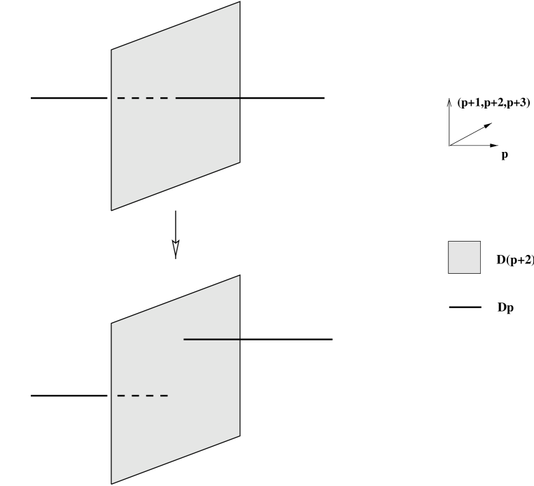
FIG. 5.: A $Dp$-brane intersecting a $D(p+2)$-brane can split into two disconnected parts which separate along the $D(p+2)$-brane.

The intersecting brane configurations discussed earlier in this section are intimately related to the configurations of branes ending on branes discussed here. As an example, when the $Dp$ and $D(p+2)$-branes of the previous subsection  meet in the transverse space $(x^{p+4},\cdots,x^{9})$, the $p$-brane can split into two parts $x^{p}<0$ and $x^{p}>0$, which can then separate along the $(p+2)$-brane in the $(x^{p+1},x^{p+2},x^{p+3})$ directions. Locally, one has then a configuration of a $p$-brane ending on a $(p+2)$-brane from the right in $x^{p}$ and another one ending on it from the left at a different place as shown in Fig. 5.

In the gauge theory on the intersection of the $Dp$ and $NS5$-branes this realizes geometrically the Higgs branch of the theory on the D-brane. This will be discussed in detail in the applications below.

III Four Dimensional Theories With $N=4$ SUSY

At low energies the dynamics on the worldvolume of $N_{c}$ parallel $D3$-branes in type IIB string theory is described by four dimensional $N=4$ SYM with gauge group $U(N_{c})$. Symplectic and orthogonal groups can be studied by considering $D3$-branes near a parallel $O3$-plane. The brane description provides a natural interpretation of the strong-weak coupling duality of $N=4$ SYM theories and leads to a simple geometrical description of BPS saturated dyons. In this section we describe this circle of ideas, starting with the unitary case.

A Montonen-Olive Duality And Type IIB S-Duality

Four dimensional $N=4$ supersymmetric gauge theory with gauge group $G$ can be obtained by dimensionally reducing $N=1$ SYM from $9+1$ to $3+1$ dimensions. SUSY (with sixteen supercharges) places strong constraints on the structure. The moduli space of vacua is $6r$ dimensional, where $r$ is the rank of $G$. It is parametrized by expectation values in the Cartan subalgebra of the six adjoint scalars in the $N=4$ multiplet. Generically in moduli space the gauge symmetry is broken to $U(1)^{r}$, but at certain singular subspaces some of the non-abelian structure is restored. The classical and quantum moduli spaces are identical in $N=4$ SYM (in contrast with $N=2$ SYM where the metric on the Coulomb branch is generally corrected by quantum effects, and $N=1$ SYM where some or all of the classical moduli space can be lifted; these cases will be discussed later). The leading quantum corrections modify certain non-renormalizable terms with four derivatives.

The most singular point in the moduli space is the origin, where the full gauge symmetry is unbroken. The theory at that point is conformal and the gauge coupling $g_{SYM}$ is an exactly marginal deformation parametrizing a line of fixed points. The theory also depends on a parameter $\theta$ which together with $g_{SYM}$ forms a complex coupling

$$\tau={\theta\over 2\pi}+{i\over g^{2}_{SYM}}$$ (62)

The theory at the origin of moduli space is conformal for all $\tau$.

Not all values of $\tau$ correspond to distinct theories. Since $\theta$ is periodic, taking $\tau\to\tau+1$ leads to the same theory. In addition, $N=4$ SYM has a less obvious symmetry, Montonen and Olive’s strong-weak coupling duality, which takes $\tau\to-1/\tau$, and exchanges the gauge algebra ${\cal G}$ with the dual algebra  ${\widehat{\cal G}}$ [169] (see [180, 127, 76] and references therein). It also acts as electric-magnetic duality on the gauge field and thus interchanges electric and magnetic charges. Together, the two symmetries generate an $SL(2,Z)$ duality group , which acts on $\tau$ by fractional linear transformations with integer coefficients:

$$\tau\longrightarrow{a\tau+b\over c\tau+d};\;\;a,b,c,d\in Z,\;ad-bc=1$$ (63)

We will mostly consider the case of an $SU(2)$ gauge group here, where states carry electric and magnetic charge under the single Cartan generator, and assemble into multiplets of $SL(2,Z)$ which contain states with electric and magnetic charges $(e,m)$ transforming under $SL(2,Z)$ as:

$$\left(\begin{array}[]{c}e\\ m\end{array}\right)\longrightarrow\left(\begin{array}[]{cc}a&b\\ c&d\end{array}\right)\left(\begin{array}[]{c}e\\ m\end{array}\right)$$ (64)

For example, the charged gauge bosons $W^{\pm}$ with charge $(\pm 1,0)$ belong to the same multiplet as the magnetic monopole with charge $(0,\pm 1)$ and various dyons.

To study $N=4$ SYM with gauge group $U(N_{c})$ using branes, consider $N_{c}$ parallel $D3$-branes, whose worldvolumes stretch in $(x^{0},x^{1},x^{2},x^{3})$. The $U(N_{c})$ gauge bosons $A_{\mu}^{a\bar{b}}(x^{\nu})$, $\mu,\nu=0,1,2,3$, $a,\bar{b}=1,\cdots,N_{c}$, correspond to the ground states of oriented $3-3$ strings connecting the $a$’th and $b$’th threebranes (Fig. 1(b)). The six scalars $X^{I}_{a\bar{b}}(x^{\mu})$ ($I=4,\cdots,9$) in the adjoint representation of $U(N_{c})$ also correspond to $3-3$ strings describing fluctuations of the threebranes in the transverse directions $(x^{4},x^{5},x^{6},x^{7},x^{8},x^{9})$. Together with the ground state fermionic fields they form an $N=4$ gauge supermultiplet.

The bosonic part of the low energy Lagrangian is given by (13, 14), with the $U(N_{c})$ gauge coupling given by $g^{2}_{SYM}=g_{s}$ (10). The conventional SYM scalar fields $\Phi^{I}$ which have dimensions of energy are related to the scalars $X^{I}$ which appear naturally in the brane construction via:

$$\Phi^{I}=X^{I}/l_{s}^{2}$$ (65)

The limit in which the theory on the threebrane decouples from gravity and the four dimensional dynamics becomes exactly that of $N=4$ SYM at all energy scales is $l_{s}\to 0$ with $g_{s}$, $\Phi^{I}$ held fixed. By the latter it is meant that the energy scale studied, $E$, and the scale set by the expectation values, $\Phi^{I}$, which typically are comparable, must be much smaller than the string scale $1/l_{s}$, and the Planck scale $1/l_{p}$ (which for $g_{s}\sim 1$ is comparable to the string scale). In particular, the transverse separations of the threebranes parametrizing the Coulomb branch must satisfy $\delta x^{i}\ll l_{s},l_{p}$.

FIG. 6.: $U(2)$ $N=4$ SYM on a pair of $D3$-branes broken to $U(1)\times U(1)$ by the separation of the branes. Dyons in SYM, such as the photon $\gamma$, the charged gauge boson $W$, and the magnetic monopole $M$, are described by $(p,q)$ strings ending on the threebranes.

In the brane picture, the $SL(2,Z)$ Montonen-Olive duality can be thought of as a remnant of the $SL(2,Z)$ S-duality group of type IIB string theory in the limit $l_{s}\to 0$. The threebrane is self-dual under S-duality. The complex worldvolume gauge coupling (62) is the expectation value of the complex type IIB dilaton $\tau$ (44) on which S-duality acts by fractional linear transformations (63), and the type IIB charges $(p,q)$ which transform under S-duality in an analogous way to (64) are related to the SYM charges $(e,m)$. In what follows we will study this correspondence in more detail in the case $N_{c}=2$.

An $N=4$ SYM gauge theory with gauge group $G=SU(2)$ is obtained in the brane description by studying the dynamics on two parallel $D3$-branes [224, 114]. Actually, the gauge group in this case is $U(2)$ but the diagonal $U(1)\subset U(2)$ will play no role in the discussion as all fields we will discuss are neutral under it; therefore it can be ignored. The six dimensional Coulomb branch of the $SU(2)$ SYM theory is parametrized by the transverse separation of the two branes ${\vec{x}}_{2}-{\vec{x}}_{1}$, where $\vec{x}\equiv(x^{4},\cdots,x^{9})$. Displacing the two threebranes from the origin by $\pm\vec{x}$ (keeping their center of mass corresponding to the decoupled $U(1)$ fixed at the origin) is equivalent to turning on a diagonal expectation value for the adjoint scalar $\vec{X}$:

$$\langle\vec{X}\rangle=\left(\begin{array}[]{cc}\vec{x}&0\\ 0&-\vec{x}\end{array}\right)$$ (66)

which breaks $SU(2)\to U(1)$.

The resulting configuration is depicted in Fig. 6. A fundamental string stretched between the two $D3$-branes corresponds to a charged gauge boson in the broken $SU(2)$ with mass given by (16). In the $N=4$ SYM theory it transforms under electric-magnetic duality (63,64) into a dyon. In the brane description S-duality takes a fundamental string to a $(p,q)$ string; thus we learn that a dyon with electric-magnetic charge $(p,q)$ corresponds in the string language to a $(p,q)$ string stretched between the two $D3$-branes.

Note that this is consistent with our discussion of branes ending on branes in section II E where we saw that a fundamental string ending on a $D3$-brane can be thought of as an electric charge in the worldvolume theory on the threebrane (60). Since S-duality acts on the threebrane as electric-magnetic duality, this implies that a D-string ending on a $D3$-brane provides a magnetic source for the threebrane worldvolume gauge field. The energy of a D-string stretched between the two $D3$-branes is $E=2|\vec{x}|/g_{s}l_{s}^{2}$ or in SYM variables $E=2|\vec{\phi}|/g^{2}_{SYM}$ as expected from gauge theory (the mass of the monopole is $M_{\rm mon}=M_{W}/g_{SYM}^{2}$ where $M_{W}$ is the mass of the charged $W$-boson).

B Nahm’s Construction Of Monopoles From Branes

FIG. 7.: A point in the moduli space of $k$ $SU(2)$ monopoles represented by D-strings stretched between $D3$-branes.

One application of this construction is to the study of the moduli space of monopoles in gauge theory. To describe the moduli space of $k$ monopoles ${\cal M}_{k}$ one is instructed to study a configuration of $k$ parallel $D1$-branes stretched between the two parallel $D3$-branes (Fig. 7), say in the $x^{6}$ direction [73]. It is easy to check that the configuration preserves eight of the sixteen supercharges of the threebrane theory, in agreement with the fact that the monopoles are $1/2$ BPS objects. The monopole moduli space ${\cal M}_{k}$ is the $4k$ real dimensional space labeled by the locations in $(x^{1},x^{2},x^{3})$ of the $k$ D-strings, and the Wilson lines of the $k$ $U(1)$ gauge fields along the D-strings, $A_{6}$.

The brane configuration suggests an alternative point of view on the space ${\cal M}_{k}$. When viewed from the point of view of the $D3$-branes it describes a moduli space of $k$ monopoles; from the point of view of the D-strings it can be thought of as the moduli space of vacua of the non-abelian gauge theory on the $k$ D-strings stretched between the $D3$-branes! That theory lives in the $1+1$ dimensions $(x^{0},x^{6})$ and, since the spatial direction $x^{6}$ is confined to a finite line segment, it reduces at low energies to Supersymmertic Quantum Mechanics. Of course, SQM does not have a moduli space of vacua, but there is an approximate Born-Oppenheimer notion of a space of vacua, which arises after integrating out all the fast modes of the system. The low energy dynamics is described by a sigma model on the moduli space ${\cal M}_{k}$.

The theory on the D-strings has eight supercharges and the following matter content. The $U(k)$ gauge field $A_{0}$ and five adjoint scalars $(\Phi^{4},\Phi^{5},\Phi^{7},\Phi^{8},\Phi^{9})$ have Dirichlet boundary conditions at $x^{6}=\pm x$ (the locations of the two threebranes). The remaining component of the D-string worldvolume gauge field $A_{6}$ and the three adjoint scalars $(\Phi^{1},\Phi^{2},\Phi^{3})$ have (formally) Neumann boundary conditions .

To study the dynamics on the worldvolume of the D-string we can set to zero all the fields which satisfy Dirichlet boundary conditions, and the gauge field $A_{6}$ (by a gauge choice). From the Lagrangian for $\Phi^{1},\Phi^{2},\Phi^{3}$ (13, 14)

$${\cal L}\sim{\rm Tr}\Big{(}\sum_{I=1}^{3}\partial_{s}\Phi^{I}\partial_{s}\Phi^{I}-\sum_{I,J}[\Phi^{I},\Phi^{J}]^{2}\Big{)}$$ (67)

(where we have denoted $x^{6}$ by $s$) it is clear that ground states satisfy

$$\partial_{s}\Phi^{I}+{1\over 2}\epsilon^{IJK}[\Phi^{J},\Phi^{K}]=0$$ (68)

The boundary conditions of the fields $\Phi^{I}$ at the edges of the interval $s=\pm x$ are interesting. Naively, one would expect that at least as long as the $k$ D-strings are widely separated in $\vec{r}=(x^{1},x^{2},x^{3})$, we should be able to think of their locations $\vec{r}_{i}$ as the expectation values of the diagonal components of the matrix fields $\vec{\Phi}_{ii}=\vec{\phi}_{i}=\vec{r}_{i}/l_{s}^{2}$ (see (15)). The off-diagonal components of $\vec{\Phi}$ are massive and could be integrated out in the Born-Oppenheimer approximation. This would lead us to deduce that the boundary conditions for the matrices $\vec{\Phi}$ are

$$\vec{\Phi}(s=\pm x)={\rm diag}(\vec{\phi}_{1},\cdots,\vec{\phi}_{k})$$ (69)

However, this picture does not make sense for finite separations of the D-strings. We saw (after (61)) that the “classical” picture of D-strings attached to the threebranes at $k$ points $\vec{r}=\vec{r}_{1},\cdots,\vec{r}_{k}$ ($\vec{r}=(x^{1},x^{2},x^{3})$) has to be replaced by a curved threebrane with $s=s(\vec{\phi})$ which approaches the classical location $s=x$ at $|\vec{\phi}|\to\infty$, but is actually described asymptotically by:

$$s\simeq\sum_{i=1}^{k}{1\over|\vec{\phi}-\vec{\phi}_{i}|}+x$$ (70)

Each D-string creates a disturbance in the shape of the threebrane of size

$$|\vec{\phi}-\vec{\phi}_{i}|\simeq{1\over s-x}$$ (71)

which diverges  as $s\to x$.

Therefore, for any finite $|\vec{\phi}_{i}-\vec{\phi}_{j}|$ (as measured in the middle of the $s$ interval) the different D-strings in fact overlap close to the edges of the $s$ interval. Hence, the off-diagonal components of the matrices $\Phi^{I}$ ($I=1,2,3$) are light and cannot be integrated out, and one expects the matrices $\Phi^{I}(s\to x)$ not to commute. The only boundary conditions for $\Phi^{I}$ that are consistent with (68, 70) are (for notational simplicity we have set the center of mass of the $k$ monopoles $\vec{r}_{0}$ to zero)

$$\Phi^{I}\simeq{T^{I}\over s-x}$$ (72)

where the $k\times k$ matrices $T^{I}$ must satisfy (68)

$$[T^{I},T^{J}]=\epsilon_{IJK}T^{K}$$ (73)

and, therefore, define a $k$ dimensional representation of $SU(2)$. The representation $T^{I}$ must furthermore be irreducible; reducible representations correspond to splitting the $k$ monopoles into smaller groups that are infinitely far apart.

As a check, we can compute the size of the bound state :

$$R^{2}=\Phi^{I}\Phi^{I}\simeq{T^{I}T^{I}\over(s-x)^{2}}={(k-1)(k+1)\over 4(s-x)^{2}}$$ (74)

i.e. $R\simeq k/2(s-x)$, roughly the size of the $k$ D-string system, as given by (70), $|\vec{\phi}|\simeq k/(s-x)$. Clearly a similar analysis holds at the other boundary of the $s$ interval, $s=-x$.

Interestingly, we have arrived (68, 72) at Nahm’s description of the moduli space of $k$ $SU(2)$ monopoles [171]! The brane realization provides a new perspective and, in particular, a physical rationale for the construction. It also makes it easy to describe generalizations, e.g. to the case of the moduli space of monopoles in higher rank groups.

Monopoles in (broken) $SU(N_{c})$ gauge theory can be discussed by considering a configuration of $N_{c}$ $D3$-branes separated in the $x^{6}$ direction, and $k_{a}$ D-strings stretched in $x^{6}$ between the $a$’th and the $a+1$’st threebrane, $a=1,\cdots,N_{c}-1$. Such configurations preserve eight supercharges and describe BPS magnetic monopoles of $SU(N_{c})$. The magnetic charge under the natural Cartan subalgebra is $(k_{1},k_{2}-k_{1},\cdots,-k_{N_{c}-1})$. The moduli space of such monopoles can be described by using a generalization of the discussion above.

C Symplectic And Orthogonal Groups From Orientifolds

To study symplectic and orthogonal groups we add an orientifold threeplane parallel to the $N_{c}$ threebranes. As described in section II B the low energy worldvolume dynamics of the $O3$ – $D3$ system is:

• $Sp(N_{c}/2)$ ($N_{c}$ even), $N=4$ SYM in $4d$ if $Q_{O3}=+{1\over 2}Q_{D3}$.

• $SO(N_{c})$, $N=4$ SYM in $4d$ if $Q_{O3}=-{1\over 2}Q_{D3}$.

In this case we can use the correspondence between gauge theory and brane theory to learn about strong coupling properties of orientifold planes, by using the correspondence between Montonen-Olive duality in gauge theory and S-duality in string theory. From gauge theory we expect $SO(2r)$ to be self-dual under $SL(2,Z)$ while $SO(2r+1)$ and $Sp(r)$ should be dual to each other. The $SO(2r)$ case works in the obvious way: the $D3$-branes and $O3$ plane are self-dual under $SL(2,Z)$. In the non-simply-laced case there is a new element. Consider a weakly coupled $SO(2r+1)$ gauge theory. The orientifold charge is $-Q_{D3}/2$; the $6r$ dimensional Coulomb branch corresponds to removing $r$ pairs of threebranes from the orientifold plane. A single threebrane which does not have a mirror remains stuck at the orientifold.

When the gauge coupling becomes large there are two ways of thinking about the system. We can either continue thinking about it as a (strongly coupled) $SO(2r+1)$ gauge theory, or relate it to a weakly coupled theory by performing a strong-weak coupling S-duality transformation. From gauge theory we know that the result should be a weakly coupled $Sp(r)$ theory, which is described by an orientifold with charge $+Q_{D3}/2$.

Thus, Montonen-Olive duality of gauge theory teaches us that a “bound state” of an $O3$-plane with negative Ramond charge and a single $D3$-brane embedded in it (a configuration with Ramond charge $(-1/2+1)Q_{D3}$) transforms under S-duality of type IIB string theory into an $O3$-plane with Ramond charge $+Q_{D3}/2$ [90].

Monopoles in broken $SO/Sp$ gauge theory are described as before by $D$-strings stretched between different $D3$-branes. Consider for example the rank one case $N_{c}=2$. For positive orientifold charge the gauge group is $Sp(1)\simeq SU(2)$ and the moduli space of $k$ $SU(2)$ monopoles that we have discussed previously can be studied by analyzing the worldvolume theory of $k$ $D$-strings connecting the single “physical” $D3$-brane to its mirror image. The gauge group $U(k)$ is replaced by $SO(k)$, and the matrices $\Phi^{I}$ (65) and $A_{6}$ become now symmetric $k\times k$ matrices. The discussion (67-73) can presumably be repeated, although this has not been done in the literature.

For negative orientifold charge the gauge group is $SO(2)\simeq U(1)$ and one does not expect non-singular monopoles to exist. This means that $D$-strings cannot connect the single physical $D3$-brane to its mirror image. This is related by S-duality to the fact, which was discussed in section II B 2, that for negative orientifold charge the ground states of fundamental strings stretched between the $D3$-brane and its image are projected out.

D The Metric On The Moduli Space Of Well-Separated Monopoles

The explicit form of the moduli space metric for $k$ well separated monopoles in $SU(2)$ gauge theory is known. Setting $g_{s}=1$, $2|\vec{x}|=1$ (66), and denoting the locations of the monopoles in $(x^{1},x^{2},x^{3})$ by $\vec{r}^{i}$ and the Wilson lines $A_{6}$ by $\theta^{i}$, so that the $4k$ dimensional monopole moduli space is labeled by $(\vec{r}^{i},\theta^{i})$, it is [107]:

$$ds^{2}=g_{ij}d\vec{r}^{i}\cdot d\vec{r}^{j}+(g^{-1})_{ij}d\tilde{\theta}^{i}d\tilde{\theta}^{j}$$ (75)

where

$$g_{jj}=1-\sum_{i\not=j}{1\over r_{ij}};\;\;\;({\rm no\;sum\;over\;}\;j)$$ (76)

$$g_{ij}={1\over r_{ij}};\;\;\;i\not=j$$ (77)

$$d\tilde{\theta}^{i}=d\theta^{i}+\vec{W}_{ik}\cdot d\vec{r}^{k}$$ (78)

$$\vec{W}_{jj}=-\sum_{i\not=j}\vec{w}_{ij};\;\;\;({\rm no\;sum\;over\;}\;j)$$ (79)

$$\vec{W}_{ij}=\vec{w}_{ij};\;\;\;(i\not=j)$$ (80)

$r_{ij}=|\vec{r}_{i}-\vec{r}_{j}|$ and $\vec{w}_{ij}$ is the vector potential of a Dirac monopole located at the point $\vec{r}_{i}$ evaluated at the point $\vec{r}_{j}$ (32).

In the brane language, one can think of the metric (75, 80) as the perturbative metric on the “Coulomb branch” of the $U(k)$ gauge theory on the D-strings. Classically, $g_{jj}=1$, $g_{ij}=0$ (for $i\not=j$). The corrections proportional to $1/r_{ij}$ in (80) arise at one loop and can be naturally interpreted as due to the asymptotic curving of the threebranes by the D-strings (61). For example, the diagonal components $g_{jj}$ can be thought of as describing the motion of the $j$’th D-string in the background of the other $k-1$ strings which curve the two threebranes such that the $\vec{r}$ dependent distance between them (for large $|\vec{r}|$) is

$$\delta x^{6}=1-\sum_{i\not=j}{1\over|\vec{r}-\vec{r}_{i}|}$$ (81)

From the point of view of the D-string theory one can interpret (81) as an $\vec{r}$ dependent gauge coupling. As we will see in section IV, for systems with eight supercharges the metric $g$ is related to the gauge coupling by SUSY. This explains the relation between (81) and the first line of (80).

Due to $(4,4)$ SUSY, there are no further perturbative corrections to the metric beyond one loop. Non-perturbatively, (80) cannot be exact, e.g. since the diagonal components of the metric are not positive definite. In the brane language, the formula for the curving of the branes (81) is only valid asymptotically for large $|\vec{r}|$ while for $|\vec{r}-\vec{r}_{i}|\to 0$, $x^{6}$ is clearly modified; instead of diverging, the two threebranes effectively “meet in the middle” of the $x^{6}$ interval. Thus, (81) must be modified.

One can think of the non-perturbative corrections to the metric (80) as due to Euclidean fundamental strings stretched between the two $D3$-branes and two adjacent D-strings (see Fig. 8). The action of such an instanton is proportional to its area,

$$S=2|\vec{x}|\delta r/l_{s}^{2}=2|\vec{\phi}|\delta r=M_{w}\delta r$$ (82)

where $2\vec{\phi}$ is the Higgs expectation value in the broken $SU(2)$ gauge theory and $\delta r$ is the separation between adjacent monopoles. The corresponding non-perturbative corrections go like $\exp(-S)\sim\exp(-M_{W}\delta r)$ where $M_{W}$ is the mass of the charged $W$-boson. This is consistent with the fact that the size of the magnetic monopole in broken $SU(2)$ gauge theory is $M_{W}^{-1}$, much larger than its Compton wavelength $M_{\rm mon}^{-1}=g_{SYM}^{2}M_{W}^{-1}$ for weak coupling $g_{SYM}$.

FIG. 8.: Non-perturbative corrections to the metric on moduli space are due to Euclidean fundamental strings stretched between the threebranes and adjacent D-strings.

Note that the instanton effects (82) are non-perturbative in $l_{s}^{2}=\alpha^{\prime}$, but they survive in the classical string limit $g_{s}\to 0$. Thus they can be thought of as worldsheet instanton corrections to the metric (80).

IV Four Dimensional Theories With $N=2$ SUSY

A Field Theory Results

The $N=2$ supersymmetry algebra contains eight supercharges transforming as two copies of the ${\bf 2}+{\bf\bar{2}}$ of $Spin(1,3)$. All $N=2$ theories have a global $SU(2)_{R}$ symmetry which acts on the two supercharges. Scale invariant theories have in addition a $U(1)_{R}$ symmetry under which the chiral supercharges have charges $\pm 1$.

To study $N=2$ supersymmetric gauge theory with gauge group $G$ one is interested in two kinds of multiplets. The vectormultiplet contains a gauge field $A_{\mu}$, two Weyl fermions $\lambda_{\alpha}$, $\psi_{\alpha}$ and a complex scalar $\phi$, all in the adjoint representation of $G$. The fermions $\lambda$, $\psi$ transform in the ${\bf 2}$ of $SU(2)_{R}$; $A_{\mu}$ and $\phi$ are singlets. Under $N=1$ SUSY the vectormultiplet decomposes into a vector superfield 

$$V=-\theta\sigma^{\mu}\bar{\theta}A_{\mu}-i\bar{\theta}^{2}(\theta\lambda)+i\theta^{2}(\bar{\theta}\bar{\lambda})+{1\over 2}\theta^{2}\bar{\theta}^{2}D$$ (83)

with the gauge covariant field strength

$$W_{\alpha}={\bar{\cal D}}^{2}\left(e^{2V}{\cal D}_{\alpha}e^{-2V}\right)$$ (84)

and a chiral superfield

$$\Phi=\phi+{\sqrt{2}}\theta\psi+\theta^{2}F$$ (85)

In $N=1$ superspace, the low energy Lagrangian describing the vectormultiplet is

$${\cal L}_{\rm vec}={\rm Im}\;{\rm Tr}\;\left[\tau\left(\int d^{4}\theta\Phi^{\dagger}e^{-2V}\Phi+\int d^{2}\theta W_{\alpha}W^{\alpha}\right)\right]$$ (86)

where the trace runs over the group $G$ and $\tau$ is the complex coupling (62). The Lagrangian (86) is invariant under the $U(1)_{R}$ symmetry $\Phi\to e^{2i\beta}\Phi(e^{-i\beta}\theta)$, which is a consequence of its (classical) conformal invariance. Thus $\Phi$ has $R$-charge two.

In components, the bosonic part of the Lagrangian ${\cal L}_{\rm vec}$ includes kinetic terms for the fields (13) and a potential for the adjoint scalars $\phi$, $\phi^{\dagger}$ analogous to (14),

$$V\sim{\rm Tr}[\phi^{\dagger},\phi]^{2}$$ (87)

$N=2$ SUSY gauge theories in four dimensions can be obtained from $N=1$ SUSY theories in six dimensions by dimensional reduction, i.e. dropping the dependence of all fields on two of the coordinates, say $(x^{4},x^{5})$. The adjoint chiral superfield in the vectormultiplet $\Phi$ (85) corresponds to $A_{4}$, $A_{5}$; the potential (87) arises from the commutator terms in the action (12).

The second multiplet of interest is the hypermultiplet, which in $N=1$ notation consists of two chiral superfields, $Q$, $\tilde{Q}$ in a representation $R$ of the gauge group (and thus contains $2{\rm dim}R$ complex scalars and Weyl fermions). The scalar components of $Q$, $\tilde{Q}$ transform as a doublet under $SU(2)_{R}$ and carry no charge under $U(1)_{R}$; the fermions are $SU(2)_{R}$ singlets and carry $U(1)_{R}$ charge one. The low energy Lagrangian describing the hypermultiplet is (in $N=1$ superspace):

$${\cal L}_{\rm hyper}=\int d^{4}\theta\left(Q^{\dagger}e^{-2V}Q+\tilde{Q}^{\dagger}e^{-2V}\tilde{Q}\right)+\int d^{2}\theta\tilde{Q}\Phi Q+{\rm c.c.}$$ (88)

where $V=V_{a}T^{a}$, $a=1,\cdots,{\rm dim}\;G$, and $T^{a}$ are generators of $G$ in the representation $R$.

The theory described by (86, 88) has a Coulomb branch corresponding to matrices $\phi$ satisfying (87) $[\phi,\phi^{\dagger}]=0$. It is parametrized by $r={\rm rank}\;G$ complex moduli corresponding to $\phi$ in the Cartan subalgebra of $G$, $\phi=\sum_{i=1}^{r}\phi_{i}T^{i}$. The gauge group is generically broken to $U(1)^{r}$ and the low energy dynamics is that of $r$ $U(1)$ vectormultiplets. $N=2$ SUSY ensures that the moduli space of vacua is not lifted by quantum effects but the metric on it is in general modified. The general form of the action consistent with $N=2$ SUSY is [217, 72, 102, 199]:

$${\cal L}_{\rm vec}={\rm Im}{\rm Tr}\left[\int d^{4}\theta{\partial{\cal F}(\Phi)\over\partial\Phi_{i}}\bar{\Phi}_{i}+{1\over 2}\int d^{2}\theta{\partial^{2}{\cal F}(\Phi)\over\partial\Phi_{i}\partial\Phi_{j}}W_{\alpha}^{i}W^{\alpha}_{j}\right]$$ (89)

${\cal F}$ is a holomorphic function of the moduli known as the prepotential. It determines the low energy $U(1)^{r}$ gauge coupling matrix $\tau_{ij}$:

$$\tau_{ij}={\partial^{2}{\cal F}\over\partial\phi_{i}\partial\phi_{j}}$$ (90)

and the metric on the moduli space

$$ds^{2}={\rm Im}\;\tau_{ij}\;d\phi_{i}d\bar{\phi}_{j}$$ (91)

Comparing to (86) we see that, classically, the prepotential is quadratic,

$${\cal F}_{0}={1\over 2}\tau_{cl}\Phi_{i}\Phi^{i}$$ (92)

After adding the one loop corrections , it takes the form:

$${\cal F}_{1}={i\over 4\pi}\sum_{\vec{\alpha}>0}(\vec{\alpha}\cdot\vec{\Phi})^{2}\log{(\vec{\alpha}\cdot\vec{\Phi})^{2}\over\Lambda^{2}}$$ (93)

where the sum runs over positive roots of the Lie algebra of $G$. The logarithm breaks $U(1)_{R}$ and is related through the multiplet of anomalies to the one loop beta function. Higher order perturbative corrections are absent due to a non-renormalization theorem, but non-perturbatively (93) receives a series of instanton corrections that fall off algebraically at large $\Phi$ but are crucial for the structure at small $\Phi$.

Seiberg and Witten showed that the prepotential ${\cal F}$ can be computed exactly and, in fact, its second derivative $\tau_{ij}$ (90) is the period matrix of a Riemann surface [208]. The moduli space of vacua of the $N=2$ SYM theory is thus parametrized by the complex structure of an auxiliary two dimensional Riemann surface whose physical role seems mysterious. One of our main goals in this section will be to elucidate the meaning of this surface by embedding the problem in string theory.

The prepotential is also important for determining the mass of BPS states in the theory. From the supersymmetry algebra one can deduce that the mass of BPS saturated states with electric charge $(e_{1},\cdots,e_{r})$ and magnetic charge $(m^{1},\cdots,m^{r})$ under the $r$ unbroken $U(1)$ gauge fields is

$$M={\sqrt{2}}|Z|;\;\;Z=\phi^{i}e_{i}+\phi_{i}^{D}m^{i}$$ (94)

where $Z$ is the central charge and

$$\phi_{i}^{D}={\partial{\cal F}\over\partial\phi^{i}}$$ (95)

In general, $N=2$ SYM theories have also Higgs branches in which the rank of the unbroken gauge group is decreased. The full phase structure is in general rather rich (see [25, 28] for a more detailed discussion). In the remainder of this section we will describe it in a few examples using branes.

B Threebranes Near Sevenbranes

As a first example of four dimensional $N=2$ SYM on branes we consider the low energy worldvolume theory on threebranes in the presence of sevenbranes and an orientifold sevenplane in type IIB string theory [33]. It can be thought of as a special case of the $Dp$ – $D(p+4)$ system of section (II) with a few special features due to the fact that $p+4=7$ is sufficiently large. In particular, the RR flux of $1+7$ dimensional objects does not have enough non-compact transverse directions to escape. Therefore, we should consider configurations with vanishing total RR charge. In this section we study a particular configuration of this sort.

Consider an $O7$-plane with worldvolume in the $(x^{0},x^{1},\cdots,x^{7})$ directions, at a point in the $(x^{8},x^{9})$ plane. Its RR charge $Q_{O7}$ is (18) $Q_{O7}=-8Q_{D7}$. To cancel this charge we can add $N_{f}=4$ $D7$-branes and their four mirror images (a total of 8 $D7$-branes with charge $Q_{D7}$ each) parallel to the orientifold sevenplane. When the $D7$-branes coincide with the orientifold plane there is an $SO(8)$ gauge symmetry on their $1+7$ dimensional worldvolume; when they are separated from the orientifold this symmetry is generically broken to $U(1)^{4}$. In a complex parameterization of the $(x^{8},x^{9})$ plane,

$$w\equiv x^{8}+ix^{9}$$ (96)

we can choose the location of the orientifold plane to be

$$w(O7)=0$$ (97)

The locations of the four $D7$-branes and their mirror partners in the $(x^{8},x^{9})$ plane will be denoted by $m_{i}$, $-m_{i}$, respectively.

In addition, we place a $D3$-brane and its mirror image at  $w$, $-w$, respectively. As explained in section II, the low energy $1+3$ dimensional worldvolume dynamics on the threebranes is an $Sp(1)\simeq SU(2)$ gauge theory with eight supercharges, namely, an $N=2$ supersymmetric gauge theory in four dimensions. The neutral gauge boson $W_{\mu}^{3}$ corresponds to the ground state of an open string both of whose ends terminate on the threebrane. The charged gauge bosons $W_{\mu}^{\pm}$ correspond to the ground states of strings stretched between the $D3$-brane and its mirror image. The $D7$-branes are heavy objects; thus from the point of view of $1+3$ dimensional physics, their $SO(8)$ gauge symmetry is “frozen,” i.e. the corresponding gauge coupling vanishes. Moduli in the sevenbrane theory give rise to parameters in the $1+3$ dimensional Lagrangian.

The location of the threebrane in the $(x^{8},x^{9})$ plane corresponds to the expectation value of the complex chiral field in the adjoint of $SU(2)$

$$\Phi_{ab}(x^{\mu})\equiv X^{8}_{ab}+iX^{9}_{ab};\qquad a,b=1,2;\qquad{\rm Tr}\;\Phi=0$$ (98)

which belongs to the $SU(2)$ vectormultiplet (85). It can be diagonalized to

$$\langle\Phi\rangle=\left(\begin{array}[]{cc}w&0\\ 0&-w\end{array}\right)$$ (99)

When $w=0$, the minimal length of strings stretched between the $D3$-branes vanishes and the charged gauge bosons are massless. When $w\neq 0$, (99) breaks $SU(2)$ to $U(1)$. Correspondingly, the strings stretched from the threebrane to its mirror image have minimal length $2|w|$ – the mass of $W^{\pm}$ (in string units).

The $D7$-branes give rise to $N_{f}=4$ fundamental hypermultiplets $(Q^{i},\tilde{Q}_{i})$. Their locations $m_{i}$ are the bare complex masses of quarks. Analyzing configurations of strings stretched between the $D3$ and $D7$-branes we see that at tree level the superpotential is just that expected on the basis of $N=2$ SUSY:

$$W=\sum_{i=1}^{4}(Q^{i}\Phi\tilde{Q}_{i}-m_{i}Q^{i}\tilde{Q}_{i})$$ (100)

The effective masses of the quarks $m_{i}-w$ and $m_{i}+w$ are the locations of the four $D7$-branes and their mirror images, respectively, relative to the $D3$-brane. The $SO(8)$ gauge symmetry on the worldvolume of the $D7$-branes turns into a global symmetry of the four dimensional gauge theory on the threebranes. It is broken when $m_{i}\neq 0$.

Just like in the $N=4$ SYM case discussed in the previous section, the complex gauge coupling of the $N=2$ SYM theory on the threebrane corresponds to the complex dilaton (44) of type IIB string theory. The $D7$-branes and $O7$-plane carry charge under the complex dilaton field. Thus it is non-trivial in their presence and, in particular, when we go once around a $D7$-brane, $\tau$ has a monodromy: $\tau\to\tau+1$. Far from the $D7$-branes that are located at $w=m_{i}$ and from the $O7$-plane located at $w=0$ we expect $\tau$ to behave as:

$$\tau(w)=\tau_{0}+{1\over 2\pi i}\Big{[}\sum_{i=1}^{4}\Big{(}\log(w-m_{i})+\log(w+m_{i})\Big{)}-8\log\,w\Big{]}$$ (101)

since there is charge $+1$ at each $w=\pm m_{i}$ and charge $-8$ at $w=0$.

Note that one can use the above analysis to understand the identification of the complex dilaton of IIB string theory (101) with the gauge coupling of the theory on the $D3$-brane. The metric on the $(x^{8},x^{9})$ plane implied by (101) can be interpreted either as the metric induced by the $O7$-plane and $D7$-branes or as the metric on the Coulomb branch of the $N=2$ SYM theory on the worldvolume of the threebrane. In the first interpretation this metric is determined by the complex coupling of type IIB string theory; in the second, it is related by (90, 91) to the complex gauge coupling $\tau$. This establishes the relation between the two $\tau$’s.

The complex coupling $\tau$ is gauge invariant; this is made manifest by rewriting (101) as

$$\tau(u)=\tau_{0}+{1\over 2\pi i}\Big{[}\sum_{i=1}^{4}\log(u-m_{i}^{2})-4\log\,u\Big{]}$$ (102)

where $u$ is the gauge invariant modulus:

$$u={1\over 2}{\rm Tr}\;\Phi^{2}=w^{2}$$ (103)

The semiclassical result (102) corresponds in gauge theory to the one loop corrected prepotential (93). As in the brane picture, semiclassically, the $SU(2)$ gauge symmetry is restored at the origin $u=0$ where $W^{\pm}$ become massless, while quarks $(Q^{i},\tilde{Q}_{i})$ become massless when $u=m_{i}^{2}$. The appearance of new massless states is the reason for the singularities at $u=0,m_{i}^{2}$ in eq. (102). The coefficient $4$ in front of $\log\,u$ is due to the fact that $W^{\pm}$ carry twice the electric charge of a quark, and the relative sign between the two logs in (102) is due to the fact that the $W^{\pm}$ belong to a vectormultiplet whose contribution to the beta function has an opposite sign to that of a hypermultiplet.

The one loop result (102) is not corrected perturbatively, but it cannot be exact, e.g. since it does not satisfy ${\rm Im}\,\tau\geq 0$ everywhere in the $u$ plane; for small $u$, ${\rm Im}\,\tau$ becomes large and negative. Therefore, we expect that strong coupling effects will modify the solution for finite $u$ [208, 209, 211]. Indeed, as discussed in section IV A, in the $N=2$ SYM analysis one finds that instanton corrections modify (102). The exact effective coupling is a modular parameter $\tau(u)$ of a torus described by the elliptic curve

$$y^{2}=x^{3}+f(u,\tau_{0})x+g(u,\tau_{0})$$ (104)

where $x,y,u\in CP^{1}$, $f(u)$ is a polynomial of degree two, $g(u)$ is a polynomial of degree three in the gauge invariant modulus $u$, and $\exp(i\pi\tau_{0})\equiv\Lambda$ is the “QCD scale” of the theory. In the semiclassical limit, namely, for large ${\rm Im}\,\tau_{0}$ and $|u|\gg|\Lambda|^{2}$, the exact $\tau(u)$ can be rewritten as (102). Strong coupling dynamics splits the singularity at the origin into two singularities at $u=\pm\Lambda^{2}$ corresponding to a monopole or dyon becoming massless.

The full non-perturbative description of the type IIB vacuum discussed above involves threebranes in F-theory on $K3$ [225] – a compactification of the IIB string on $CP^{1}$ labeled by the coordinate $u$, with a non-trivial complex dilaton describing a two-torus with modular parameter $\tau(u)$ for each point on $CP^{1}$. This elliptically fibered surface is given by the algebraic equation (104).

In the F-theory description the threebrane moves in the background of six sevenbranes located at the singularities of the curve (104). In the weak string-coupling limit four of these branes can be regarded as $(1,0)$ sevenbranes, namely, conventional D-branes, while the other two are a $(0,1)$ sevenbrane and a $(2,1)$ sevenbrane related to a $D7$-brane by $SL(2,Z)$ S-duality transformations. The $(1,0)$ sevenbranes are free to move in the $u$ plane, while the $(0,1)$ and $(2,1)$ sevenbranes are stuck at $u=\pm\Lambda^{2}$. As $g_{s}\to 0$ these branes approach each other and are described at weak coupling by an $O7$-plane. BPS saturated states with electric and magnetic charges $(e,m)=(p,q)$ in the four dimensional $N=2$ SYM theory on the threebrane can be described by $(p,q)$ strings stretched between the $(p,q)$ sevenbranes and the $D3$-brane [212].

C Branes Suspended Between Branes

The fact that branes can end on other branes was deduced in subsection II E 3 by starting from a fundamental string ending on a D-brane and applying U-duality. Following the same logic we can deduce that branes can be suspended between other branes by starting with a configuration of fundamental strings stretched between two D-branes and applying a chain of duality transformations. As in subsection II E 3, one can get this way $Dp$-branes stretched between two $D(p+2)$ or $NS5$-branes. The special case of D-strings stretched between two $D3$-branes was used in section III to describe BPS saturated ‘t Hooft-Polyakov monopoles of a broken $SU(2)$ gauge theory.

In this section we will study similar configurations with eight supercharges describing $3+1$ dimensional physics, and use them to learn about $N=2$ SYM. The starting point of our discussion will be brane configurations in type IIA string theory consisting of solitonic (NS) fivebranes, $D4$-branes and $D6$-branes as well as orientifold planes $O4$ and $O6$ parallel to the D-branes. Using eqs. (8, 24, 26) it is not difficult to check that any combination of two or more of the following objects:

$$\begin{array}[]{ll}\mbox{$NS5:$}&\mbox{$(x^{0},x^{1},x^{2},x^{3},x^{4},x^{5})$}\\ \mbox{$D4/O4:$}&\mbox{$(x^{0},x^{1},x^{2},x^{3},x^{6})$}\\ \mbox{$D6/O6:$}&\mbox{$(x^{0},x^{1},x^{2},x^{3},x^{7},x^{8},x^{9})$}\end{array}$$ (105)

preserves eight of the thirty two supercharges of IIA string theory (4). In eq. (105) we specified the directions in which each of the branes is stretched.

The Lorentz group $SO(1,9)$ is broken by the presence of the branes to:

$$SO(1,9)\longrightarrow SO(1,3)\times SO(2)\times SO(3)$$ (106)

where the $SO(1,3)$ factor acts on $(x^{0},x^{1},x^{2},x^{3})$, the $SO(2)$ on $(x^{4},x^{5})$ and the $SO(3)$ on $(x^{7},x^{8},x^{9})$. We will be interested in physics in the $1+3$ dimensional spacetime common to all the branes labeled by $(x^{0},x^{1},x^{2},x^{3})$; thus we interpret the $SO(1,3)$ factor in (106) as Lorentz symmetry and the $SO(2)$, $SO(3)$ factors as global symmetries. Due to the ten dimensional origin of these global symmetries, the supercharges transform as doublets under $SO(3)$, and are charged under $SO(2)$. Thus, these are $R$-symmetries. In fact, the $SO(3)$ can be identified with the global $SU(2)_{R}$ of $N=2$ SYM described in section IV A while the $SO(2)$ can be identified with the $U(1)_{R}$ symmetry.

To study situations with interesting $1+3$ dimensional physics some of the branes must be made finite. We next turn to a discussion of some specific configurations and their physics [123, 87]. We start with a description of the “classical” type IIA string picture in a few cases involving unitary, symplectic and orthogonal groups with matter in the fundamental representation of the gauge group, as well as a few more complicated examples, and then study quantum effects.

1 Unitary Gauge Groups

Consider two infinite $NS5$-branes oriented as in (105), separated by a distance $L_{6}$ in the $x^{6}$ direction and located at the same point in $(x^{7},x^{8},x^{9})$. We can stretch between them in the $x^{6}$ direction $N_{c}$ $D4$-branes oriented as in (105); see Fig. 9.

FIG. 9.: $N_{c}$ $D4$-branes stretched between $NS5$-branes describe $N=2$ SYM with $G=U(N_{c})$.

To analyze the low energy physics corresponding to this configuration it is important to distinguish between three kinds of excitations of the vacuum: 1) modes that live in the ten dimensional bulk of spacetime; 2) modes that live on the two $NS5$-branes; 3) modes that live on the fourbranes. For an observer living in the $1+3$ dimensions $(x^{0},x^{1},x^{2},x^{3})$ the first two sets of excitations appear at low energies and in the weak string coupling limit to be frozen at their classical values by an argument similar to that given around eq. (57). Essentially, since they correspond to higher dimensional excitations any long wavelength fluctuations away from the classical values of these fields are suppressed by infinite volume factors.

Excitations attached to the $N_{c}$ fourbranes do not have this property. Despite living in one higher dimension ($x^{6}$), they are dynamical in $1+3$ dimensions since the fourbranes are finite in $x^{6}$. Thus excitations of the fourbranes can be thought of as fields living in the $1+4$ dimensional space $R^{1,3}\times I$ where $I$ is a finite interval (of length $L_{6}$). Just like in Kaluza-Klein theory, for distance scales much larger than $L_{6}$ their physics looks $1+3$ dimensional. Depending on the boundary conditions at the ends of the interval, the different fields do or do not give rise to light fields in $1+3$ dimensions.

The analysis of the boundary conditions can be done using the results of subsection II E 3. The light excitations on a stack of $N_{c}$ infinite $D4$-branes (105) are a five dimensional $U(N_{c})$ gauge field $A_{\mu}$, $\mu=0,1,2,3,6$ and five scalars in the adjoint of $U(N_{c})$ corresponding to transverse fluctuations of the fourbranes, $(X^{4},X^{5},X^{7},X^{8},X^{9})$. As we saw in subsection II E 3, when the $N_{c}$ fourbranes end on fivebranes, $(X^{7},X^{8},X^{9})$ as well as $A_{6}$ satisfy Dirichlet boundary conditions on both ends of the interval $I$. Therefore, they give rise in $1+3$ dimensions to states with masses of order $1/L_{6}$, which are invisible in the low energy limit of interest, $E\ll 1/L_{6}$. The remaining light degrees of freedom, the $U(N_{c})$ gauge field $A_{\mu}$, $\mu=0,1,2,3$ and the adjoint scalars $(X^{4},X^{5})$, satisfy free boundary conditions on $I$ and, therefore, contribute a $U(N_{c})$ vectormultiplet.

Thus, we conclude that the light excitations of the brane configuration above describe an $N=2$ SUSY gauge theory with gauge group $U(N_{c})$ and no matter . The gauge coupling of the $4+1$ dimensional gauge theory on $N_{c}$ fourbranes is given by standard D-brane techniques (10) to be $g_{D4}^{2}=g_{s}l_{s}$. Upon Kaluza-Klein reduction on a line segment of length $L_{6}$ we find a $3+1$ dimensional gauge theory with coupling

$${1\over g^{2}}={L_{6}\over g_{s}l_{s}}$$ (107)

It is interesting to ask in what regime the brane configuration is well approximated by an $N=2$ SUSY $3+1$ dimensional gauge theory. There are several issues that need to be addressed in this regard. First, the physics on the fourbranes looks $3+1$ dimensional only at distances much larger than $L_{6}$. At shorter distances Kaluza-Klein excitations on the fourbranes, whose typical energy is $1/L_{6}$, begin to play a role and the dynamics becomes $4+1$ dimensional. Furthermore, in general there are couplings of the light fields on the fourbranes to light fields living on the $NS5$-branes, to massive excited states of the $4-4$ strings living on the fourbranes, and to fields living in the bulk of spacetime, such as gravitons. These coupling are small in the limit $g_{s}\to 0$ and at distances much larger than $l_{s}$.

Thus to study gauge theory dynamics we are led to consider the brane configuration above in the limit

$$g_{s}\to 0,\;\;\;L_{6}/l_{s}\to 0$$ (108)

with the ratio corresponding to $g$ (107) held fixed. If the gauge coupling at some scale $L$ satisfying $L\gg l_{s}\gg L_{6}$ is small but finite, at larger distances the dynamics of the brane configuration will be governed by gauge theory with the other effects mentioned above providing small corrections.

The classical gauge theory limit is obtained when in addition to sending $L_{6}$ and $g_{s}$ to zero, we also send the combination (107) to zero. The theory simplifies in this limit, since when $g=0$ we can ignore the effects of the ends of the fourbranes on the $NS5$-branes. In this subsection we will discuss this classical limit; later we will describe the modifications that take place when quantum effects are turned on.

Classical $U(N_{c})$ $N=2$ SYM in $3+1$ dimensions has an $N_{c}$ (complex) dimensional moduli space of vacua parametrized by diagonal expectation values of the complex adjoint scalar $\Phi$ that belongs to the vectormultiplet. At a generic point in the moduli space, $U(N_{c})$ is broken to $U(1)^{N_{c}}$ and the charged gauge bosons are massive.

In the brane description, the complex adjoint field $\Phi$ (85) can be thought of as describing fluctuations of the fourbranes along the fivebranes, $X\equiv\Phi l_{s}^{2}=X^{4}+iX^{5}$. Turning on an expectation value for $\Phi$ corresponds to translations of the $N_{c}$ fourbranes in $x^{4}$, $x^{5}$. For generic positions of the fourbranes along the fivebranes, the $4-4$ strings connecting different fourbranes (corresponding to vectormultiplets charged under a pair of $U(1)$’s) have finite length and, therefore, describe massive states. Note also that $\Phi$ has the correct global charges. Turning on an expectation value for $\Phi$ breaks the $SO(2)$ symmetry (106). Thus, $\Phi$ carries charge (which is two if we normalize the charge of the supercharges to one) under $U(1)_{R}$. Similarly, it is clear that it transforms as a singlet under $SO(3)\simeq SU(2)_{R}$; both facts are in agreement with the field theory discussion of section IV A.

To have a consistent four dimensional interpretation of the Coulomb branch we have to require that in the limit (108) the Higgs expectation value $\langle\Phi\rangle$ must remain well below the Kaluza-Klein scale $1/L_{6}$. This means that the typical separation between the fourbranes in the $(x^{4},x^{5})$ plane $\delta x$ must satisfy $\delta x\ll l_{s}^{2}/L_{6}$. One should also require that $\delta x\ll l_{s},L_{6}$ to decouple massive string modes on the fourbranes. The resulting hierarchy of scales in the gauge theory limit (108) is

$$\delta x\ll L_{6}\ll l_{s}\ll{l_{s}^{2}\over L_{6}}$$ (109)

FIG. 10.: $N_{c}$ “color fourbranes” stretched between $NS5$-branes in the presence of $N_{f}$ semi-infinite “flavor fourbranes” describe $N=2$ SYM with $G=U(N_{c})$ and $N_{f}$ fundamental hypermultiplets.

To add matter in the fundamental representation of the gauge group we can proceed in one of a number of related ways. One is to add semi-infinite fourbranes attached to one of the $NS5$-branes. For example, one can add $N_{f}$ fourbranes ending on the left $NS5$-brane from the left, extending to $x^{6}\to-\infty$, as shown in Fig. 10. Adding the semi-infinite fourbranes gives rise to $N_{f}$ hypermultiplets in the fundamental representation of $U(N_{c})$ corresponding to strings stretched between the $N_{c}$ suspended fourbranes and the $N_{f}$ semi-infinite ones. The locations at which these semi-infinite fourbranes attach to the fivebrane in the $(x^{4},x^{5})$ plane are $N_{f}$ complex numbers $m_{1},\cdots,m_{N_{f}}$ which can be thought of as the masses of the quarks . Note that these locations correspond to expectation values of scalar fields living on the worldvolume of the semi-infinite fourbranes. As before, since these fourbranes are “heavy” objects, they are frozen at their classical values and give rise to couplings rather than moduli in the four dimensional low energy theory.

A generic point in the Coulomb branch is parametrized by the $N_{c}$ complex numbers $a^{1},\cdots,a^{N_{c}}$ corresponding to the locations in the $(x^{4},x^{5})$ plane of the suspended $D4$-branes. From gauge theory we know that due to the superpotential (100) (with the sum running over all $N_{f}$ flavors) which is required by $N=2$ SUSY, the mass of the quark $Q^{i}_{\alpha}$ corresponding to the $i$’th flavor and the $\alpha$’th color is $m_{i}^{\alpha}=|m_{i}-a^{\alpha}|$. In the brane picture, the mass $m_{i}^{\alpha}$ is given by the minimal energy of a fundamental string stretched between the $\alpha$’th suspended brane and the $i$’th semi-infinite one. Just like the adjoint field $\Phi$, the mass parameters $m_{i}$ (100) carry $U(1)_{R}$ charge two. Turning on masses breaks $U(1)_{R}$ (as well as conformal invariance).

While the above way of introducing fundamental matter is appropriate for describing the Coulomb branch of $U(N_{c})$ gauge theory with $N_{f}$ flavors, it does not provide a geometric description of the Higgs branches. Recall that the gauge theory in question has a number of branches of the moduli space of vacua along which some of the quarks $Q$, $\tilde{Q}$ get expectation values and the rank of the unbroken gauge group decreases. For $N_{f}\geq 2N_{c}$ the gauge group can be completely Higgsed and the complex dimension of the corresponding branch of moduli space is $2N_{c}N_{f}-2N_{c}^{2}$.

To recover the Higgs branches it is convenient to generalize the above construction of matter in a way shown in Fig. 11. Replace the semi-infinite $D4$-branes to the left of the $NS5$-branes by finite $D4$-branes each ending on a different $D6$-brane oriented as in (105). This opens up the possibility of having additional dynamical degrees of freedom living on these fourbranes.

FIG. 11.: Replacing the semi-infinite flavor $D4$-branes of Fig. 10 by $D4$-branes ending on $D6$-branes allows one to explore the full phase structure of the theory.

For generic masses $\{m_{i}\}$ (which can now be thought of as positions of the $N_{f}$ $D6$-branes in the $(x^{4},x^{5})$ plane) and points in the Coulomb branch $\{a^{\alpha}\}$, there are no new massless states of this kind. Indeed, all potentially light fields living on a fourbrane stretched between an $NS5$-brane and a $D6$-brane have Dirichlet boundary conditions on one or both boundaries and hence do not lead to massless degrees of freedom. That is consistent with the absence of Higgs branches of $N=2$ SYM when all the masses $m_{i}$ are distinct.

When two or more masses coincide, say $m_{1}=m_{2}$ we expect from gauge theory to be able to enter a Higgs branch by turning on an expectation value to quarks $Q$, $\tilde{Q}$. Furthermore, to enter the Higgs branch one needs to go to a particular point in the Coulomb branch for which for some $1\leq\alpha\leq N_{c}$, $m_{1}^{\alpha}=m_{2}^{\alpha}=0$. To reproduce this in the brane description one notes that when two masses $m_{i}$ coincide, two $D6$-branes are at the same position in the $(x^{4},x^{5})$ plane. In general they are still separate in the $x^{6}$ direction and each is connected to the same $NS5$-brane by a $D4$-brane. Thus the fourbrane connecting the “far” $D6$-brane to the $NS5$-brane meets in space and intersects the “near” $D6$-brane. From our discussion of brane intersections in subsection II E 3 one might conclude at this point that this fourbrane can break into two pieces, one stretched between the $NS5$-brane and the near $D6$-brane and the other between the two $D6$-branes. While the first piece would as before give rise to no massless degrees of freedom in $3+1$ dimensions, the second one would in fact give rise to a neutral (under the gauge group) massless hypermultiplet. The scalars in the hypermultiplet would correspond to displacements of the $D4$-brane along the $D6$-branes in the $(x^{7},x^{8},x^{9})$ directions, and the compact component of the gauge field $A_{6}$. This would provide a candidate for a brane realization of the phase transition from the Coulomb to the Higgs phase.

However, the picture we got so far is inconsistent with gauge theory. The process described above appears to be possible for any values of the Coulomb moduli; in gauge theory we have to tune to a particular point in the Coulomb branch in order to be able to enter the Higgs branch. This and many related puzzles are resolved by noting [123] that the following “s-rule” holds in brane dynamics:

A configuration in which an NS fivebrane and a D sixbrane are connected by more than one $D4$-brane is not supersymmetric.

The s-rule, which is illustrated in Fig. 12, is a phenomenological rule of brane dynamics which has been recently discussed from various points of view, for example, in [182, 132, 31, 30]. It seems to have to do with the fact that two or more fourbranes connecting a given NS fivebrane to a given D sixbrane are necessarily on top of each other – a rather singular situation. In particular, in [31, 30] it has been related by U-duality to Pauli’s exclusion principle.

FIG. 12.: (a) A supersymmetric configuration containing an $NS5$-brane connected to a $D6$-brane by a single $D4$-brane. (b) A non-supersymmetric configuration in which the two are connected by two $D4$-branes.

The s-rule explains why the process described above is forbidden, but the comparison to the gauge theory picture suggests a way out. If in addition to having two $D6$-branes coincide in the $(x^{4},x^{5})$ plane we also go to a point in the Coulomb branch where one of the $N_{c}$ $D4$-branes suspended between the NS-branes is at the same value of $(x^{4},x^{5})$ as well, the above phase transition becomes possible (Fig. 13).

FIG. 13.: The transition from Coulomb (a) to Higgs (b) branch.

All we have to do is first reconnect the $D4$-brane stretched between the left $NS5$-brane and the far $D6$-brane, combining it with the coincident $D4$-brane suspended between the NS-branes such that it now connects the right $NS5$-brane to the far $D6$. Now there is no conflict with the s-rule in breaking the resulting stretched $D4$ into two pieces as described above. As expected in the Higgs mechanism, in the process we replace a massless $U(1)$ vectormultiplet corresponding to a $D4$-brane stretched between two $NS5$-branes by a massless neutral hypermultiplet $\tilde{Q}Q$ corresponding to a $D4$-brane stretched between adjacent (in $x^{6}$) $D6$-branes. The expectation value $\langle\tilde{Q}Q\rangle$ is parametrized by the location of this $D4$-brane along the $D6$-branes in $(x^{7},x^{8},x^{9})$ and the Wilson line of $A_{6}$. This is consistent with the expected transformation of $Q$, $\tilde{Q}$ under $SU(2)_{R}\times U(1)_{R}$: they are not charged under $U(1)_{R}$ and transform as a doublet under $SU(2)_{R}$. Thus the “mesons” $\tilde{Q}Q$ transform as ${\bf 2}\times{\bf 2}={\bf 3}+{\bf 1}$.

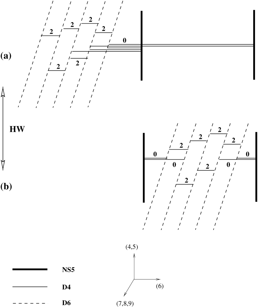
FIG. 14.: The fully Higgsed branch of moduli space for $N_{f}=5$, $N_{c}=2$; the two equivalent descriptions are related by a series of HW transitions.

Thus we learn that the Higgs mechanism is described in brane theory as the reconnection (or breaking) of $D4$-branes stretched between $NS5$-branes which give rise to vectormultiplets into ones stretched between $D6$-branes and/or $NS5$-branes consistently with the s-rule. Performing all such breakings in the general case of $N_{c}$ colors and $N_{f}$ flavors gives rise to the correct (classical) phase structure of $N=2$ SYM.

As an example, to compute the dimension of the maximally Higgsed branch (where the gauge symmetry is completely broken) for $N_{f}\geq 2N_{c}$ we proceed as follows (see Fig. 14(a)):

• Set all the masses equal to each other, i.e. bring all $N_{f}$ $D6$-branes to the same point in $(x^{4},x^{5})$, say the origin. They are still at different positions in $x^{6}$.

• Reconnect the $D4$-brane stretching between the left $NS5$-brane and the leftmost $D6$-brane to stretch between the right $NS5$ and the leftmost $D6$, by going to the point in the Coulomb branch where one of the $N_{c}$ “color” $D4$’s is at the origin in the $(x^{4},x^{5})$ plane as well.

• Break the resulting $D4$ into $N_{f}$ pieces stretching between the right $NS5$ and the rightmost $D6$ and the different adjacent $D6$’s. This leads to $N_{f}-1$ massless hypermultiplets corresponding to fluctuations of the $N_{f}-1$ segments of the $D4$ stretched between the $D6$’s. The expectation values of these are $2(N_{f}-1)$ complex moduli.

• By bringing in another color $D4$, reconnect the “second longest” $D4$ stretching between the left $NS5$ and the next to leftmost $D6$ to the right $NS5$. Repeat the breaking procedure. The s-rule applied to the right $NS5$ implies that there are now $N_{f}-3$ massless hypermultiplets and hence $2(N_{f}-3)$ complex moduli.

• Continuing this process gives rise to

  $$\sum_{i=1}^{N_{c}}(N_{f}-(2i-1))=N_{f}N_{c}-N_{c}^{2}$$ (110)

  massless hypermultiplets and to a $2(N_{f}N_{c}-N_{c}^{2})$ complex dimensional Higgs moduli space, in agreement with gauge theory expectations.

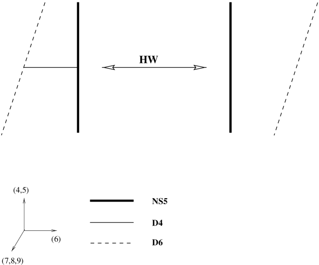
FIG. 15.: The HW transition, in which a fourbrane is created when an $NS5$-brane and a $D6$-brane cross in $x^{6}$ and exchange positions.

A peculiar feature of the above analysis is the (lack of) role of the parameters describing the positions along the $x^{6}$ axis of the $N_{f}$ $D6$-branes providing the flavors. There are no parameters in the low energy $N=2$ SQCD corresponding to changing these parameters and thus they are irrelevant (in the RG sense). Indeed, the physics of the brane configuration is independent of the locations of the $D6$-branes at least when they are all to the left (or equivalently all to the right) of the two $NS5$-branes.

It is interesting to ask what happens if we try to vary the $x^{6}$ positions of the $D6$-branes, bringing some or all of them inside the interval between the two NS-branes. Because of the way the different branes are oriented (105) the $D6$ and $NS5$-branes cannot avoid each other, and when their $x^{6}$ values coincide they actually meet in space. What takes place when they switch positions is known as the “HW transition” [123]. The $D4$-brane connecting the $D6$ and $NS5$ becomes very short as they approach each other and disappears when they cross. Conversely, if the $D6$ and $NS5$ that approach each other do not have a $D4$-brane connecting them, one is created when they exchange positions (Fig. 15).

The HW transition is an interesting effect of brane dynamics which is related by U-duality to similar transitions for other branes; it was further investigated from several perspectives, for example, in [182, 29, 63, 40, 64, 130, 179, 41, 175, 240]. Heuristically, it is related to conservation of a certain magnetic charge which can be measured on each brane known as the “linking number.” The total charge measured on each brane is

$$L_{B}={1\over 2}(r-l)+L-R$$ (111)

For an $NS5$-brane, $r$ and $l$ are the numbers of $D6$-branes to its right and left, respectively, while $R$ and $L$ are the numbers of $D4$-branes ending on the $NS5$-brane from the right and left, respectively. Similarly, for a $D6$-brane $r$ and $l$ are the numbers of $NS5$-branes to its right and left, and $R$ and $L$ are as above. Right and left here refer to locations along the $x^{6}$ axis.

As an example, for a $D6$-brane connected to an $NS5$-brane on its right (in $x^{6}$) by a $D4$-brane the linking number is $L_{D6}=-1/2$. For the $NS5$-brane the linking number is $L_{NS5}=+1/2$. If we try to move the $D6$-brane past the $NS5$-brane the $D4$ connecting them disappears. The new configuration includes a $D6$ with a disconnected $NS5$ on its left; the linking numbers are seen from (111) to be unchanged.

Taking the HW transition into account we can analyze what happens when the $D6$-branes are translated in the $x^{6}$ direction and placed in the interval between the two NS-branes. All the $D4$-branes that initially connected the $D6$-branes to an $NS5$-brane disappear, and we end up with a configuration of two NS-branes at different values of $x^{6}$ connected to each other by $N_{c}$ fourbranes, with $N_{f}$ sixbranes located between them in $x^{6}$ (see Fig. 14(b)).

Remarkably, the resulting brane configuration describes the same low energy physics! This is a priori surprising since one would in general expect a phase transition to occur as the two branes cross; indeed, we will see that such transitions occur when the crossing branes are parallel. It is not well understood why there is no phase transition when non-parallel branes cross.

In any case, in the present setup the quarks $Q$, $\tilde{Q}$ that corresponded to $4-4$ strings before are now due to $4-6$ strings stretched between the $N_{c}$ suspended fourbranes and the $N_{f}$ sixbranes. The locations of the sixbranes in the $(x^{4},x^{5})$ plane still correspond to their masses, and the Higgs branch of the moduli space is described by breaking $D4$-branes stretched between the two $NS5$-branes on the $N_{f}$ $D6$-branes. Taking into account the s-rule it is easy to see that the dimension of the Higgs branch is as described above (110).

The $N=2$ SYM theory under consideration has gauge group $U(N_{c})\simeq SU(N_{c})\times U(1)$. Thus one can turn on Fayet-Iliopoulos (FI) couplings for the $U(1)$. In $N=1$ superspace they are an $N=1$ FI D-term, and a linear superpotential for the adjoint chiral superfield in the vectormultiplet:

$${\cal L}_{FI}={\rm Tr}\;\left(r_{3}\int d^{4}\theta V+r_{+}\int d^{2}\theta\Phi+r_{-}\int d^{2}\bar{\theta}\bar{\Phi}\right)$$ (112)

$r_{3}$ is real, while $r_{+}^{*}=r_{-}$. The three FI couplings $r_{3},r_{\pm}$ transform as the ${\bf 3}$ of $SU(2)_{R}$ and are neutral under $U(1)_{R}$. For $N_{f}\geq N_{c}$ the D-terms break the gauge group completely and force the system into the Higgs branch. For smaller $N_{f}$ there is no supersymmetric vacuum.

In the brane language, the FI couplings correspond to the relative position of the two $NS5$-branes in the $(x^{7},x^{8},x^{9})$ directions (Fig. 16); note that these parameters have the correct transformation properties under $SO(3)\simeq SU(2)_{R}$. From the geometry and (105) it is clear that only when the two $NS5$-branes are at the same value of $(x^{7},x^{8},x^{9})$ can the $D4$-branes stretch between them without breaking SUSY. For non-zero D-terms all the $D4$-branes must break on $D6$-branes. This corresponds to complete Higgsing of the gauge group; it is consistent with the s-rule for $N_{f}\geq N_{c}$; for smaller $N_{f}$ there is no supersymmetric vacuum.

FIG. 16.: FI D-terms in the $N=2$ SYM theory correspond to relative displacements of the two $NS5$-branes in $(x^{7},x^{8},x^{9})$. For non-zero D-terms, all color $D4$-branes must break and the theory is forced into the Higgs phase.

2 Orthogonal And Symplectic Groups

In this subsection we will discuss configurations of branes near orientifold planes. As we saw before, adding orientifold four and six ($O4$ and $O6$) planes as in (105) does not lead to the breaking of any further SUSY, or global symmetry (106). In the simplest cases one finds $N=2$ SYM theories with orthogonal and symplectic gauge groups and matter in the fundamental representation. We next discuss in turn the two cases of an $O6$-plane parallel to the $D6$-branes and of an $O4$-plane parallel to the $D4$-branes.

1. Orientifold Sixplanes

Consider a configuration in which an $NS5$-brane is placed at a distance $L_{6}$ from an orientifold sixplane (all objects here and below oriented as in (105)). We would like to stretch $D4$-branes between the $NS5$-brane and the orientifold plane (a useful way to think about these is as $D4$-branes stretched between the $NS5$-brane and its mirror image with respect to the orientifold). As discussed in section II B, there are actually two different kinds of $O6$-planes, with positive and negative charge.

The first question we have to address is whether we can stretch $D4$-branes between the $NS5$-brane and its image in this situation without breaking SUSY. One might worry that such fourbranes are projected out by the orientifold projection for one of the two possible choices of the orientifold charge. For example, we will see later that it is impossible to stretch a BPS saturated $D4$-brane between a $D6$-brane parallel to an $O6_{-}$ plane and its image, and this will have important consequences for the low energy gauge theory. We next show that for the case of $NS5$-branes there is no such obstruction.

U-duality relates the configuration we have to a more familiar one . Specifically we perform a T-duality transformation (54) $T_{123}$ which takes the type IIA string theory to a type IIB one, followed by an S-duality transformation $S$ (55) on the resulting IIB string. $T_{123}$ maps the $NS5$-brane to itself, the $O6$-plane to an $O3$-plane $(x^{0},x^{7},x^{8},x^{9})$ and the $N_{c}$ $D4$-branes to $N_{c}$ D-strings stretched in $x^{6}$ between the two fivebranes. The subsequent S-duality transformation acts differently for positive and negative orientifold charge.

For negative orientifold charge, we saw in section III that the $O3$-plane transforms under $S$ to itself. Thus after performing the transformation, we end up with a $D5$-brane and its image near an $O3_{-}$ plane. The original $D4$-branes connecting the $NS5$-brane to its image turn now into fundamental IIB strings connecting the $D5$-brane to its image with respect to the $O3$-plane. The low energy theory on the $D5$-brane is in this case an $SO(2)$ gauge theory; the configuration is T-dual to well studied systems such as D-strings inside an $O9$-plane or $D0$-branes near an $O8$-plane. Translations of the D-brane and its image away from the orientifold plane (in the $x^{6}$ direction) are described by an antisymmetric tensor of $SO(2)$, i.e. a singlet.

The original question, whether one can stretch a $D4$-brane between the $NS5$-brane and its mirror, is translated in the U-dual configuration into the question whether one can stretch a BPS saturated string between the $D5$-brane and its image. Such a string would correspond to a state charged under the $SO(2)$ gauge symmetry on the $D5$-brane, that goes to zero mass as the $D5$-brane approaches its image. It is well known that such states exist; they correspond to fields describing fluctuations of the D-brane along the orientifold plane, in this case in the $(x^{7},x^{8},x^{9})$ directions. Such fluctuations are described by a symmetric tensor of $SO(2)$ which includes a pair of states charged under $SO(2)$; these states are described by BPS fundamental strings stretched between the $D5$-branes. They are U-dual to $D4$-branes connecting the $NS5$-brane to its image in the original configuration. In particular, the latter is clearly possible.

For positive orientifold charge we use the fact – explained in section III – that S-duality takes an $O3_{+}$ plane to an $O3_{-}$ plane with a single $D3$-brane (without a mirror partner) embedded in it. The resulting system of a $D5$-brane near an $O3_{-}$ plane with a $D3$-brane is similar to that studied in the previous paragraphs. The $D3$-brane gives rise to additional matter which plays no role in the discussion. Clearly the rest of the analysis can be repeated as above, with the same conclusions – it is possible to stretch $D4$-branes between an $NS5$-brane and its image with respect to an $O6$-plane of either sign.

We will next describe the classical gauge theories corresponding to the two choices of the sign of the orientifold charge, starting with the case of positive $O6$ charge (Fig. 17), which leads to an orthogonal projection on the $D4$-branes. The case of $O6_{-}$, which leads to a symplectic gauge group, will be considered later.

FIG. 17.: The Coulomb, (a), and fully Higgsed, (b), branches of moduli space of $SO(2)$ gauge theory with $N_{f}=3$ charged hypermultiplets.

The gauge group on $N_{c}$ $D4$-branes connecting an $NS5$-brane to its mirror image with respect to an $O6_{+}$ plane is $SO(N_{c})$. $N_{f}$ $D6$-branes parallel to the $O6$-plane located between the $NS5$-brane and the orientifold give $N_{f}$ hypermultiplets in the fundamental (${\bf N_{c}}$) representation of $SO(N_{c})$, arising as usual from $4-6$ strings. In $N=1$ SUSY notation there are $2N_{f}$ chiral multiplets $Q^{i}$, $i=1,\cdots,2N_{f}$, which are paired to make $N_{f}$ hypermultiplets. The global flavor symmetry of this gauge theory is $Sp(N_{f})$, in agreement with the projection imposed by the positive charge $O6$-plane on the $D6$-branes.

The Coulomb branch of the $N=2$ SUSY gauge theory is parametrized by the locations of the $D4$-branes along the fivebrane in the $(x^{4},x^{5})$ plane. Entering the Coulomb branch involves removing the ends of the fourbranes from the orientifold plane (which is located at a particular point in the $(x^{4},x^{5})$ plane). Since the fourbranes can only leave the orientifold plane in pairs, the dimension of the Coulomb branch is $[N_{c}/2]$, in agreement with the gauge theory description.

Higgs branches of the gauge theory are parametrized by all possible breakings of fourbranes on sixbranes. As for the unitary case there are many different branches; as a check that we get the right structure, consider the fully Higgsed branch which exists when the number of flavors is sufficiently large. From gauge theory we expect its dimension to be $2N_{c}N_{f}-N_{c}(N_{c}-1)$.

The brane analysis gives

$${\rm dim}{\cal M}_{H}=\sum_{i=1}^{N_{c}}2(N_{f}+1-i)=2N_{f}N_{c}-N_{c}(N_{c}-1)=[2N_{f}N_{c}-N_{c}(N_{c}+1)]+2N_{c}$$ (113)

The number in the square brackets is the number of moduli corresponding to segments that do not touch the orientifold, and the additional $2N_{c}$ is the number of moduli coming from the segments of the fourbranes connecting the $D6$-brane closest to the orientifold to its mirror image. These segments transform to themselves under the orientifold projection and thus are dynamical for positive orientifold charge. An example is given in Fig. 17(b).

The $2N_{c}$ moduli coming from fourbranes connecting a $D6$-brane to its image have a natural interpretation in the theory on the $D6$-branes. At low energies this is an $Sp(1)$ gauge theory with sixteen supercharges, and the $D4$-branes stretched between the $D6$ and its mirror can be thought of as $Sp(1)$ monopoles, as in section III. From this point of view the above $2N_{c}$ moduli parametrize the space of $N_{c}$ $Sp(1)$ monopoles.

Thus, the total dimension of moduli space agrees with the gauge theory result. It is easy to similarly check the agreement with gauge theory of the maximally Higgsed branch for small $N_{f}$, as well as the structure of the mixed Higgs-Coulomb branches.

For negative charge of the $O6$-plane, the configuration of Fig. 18 describes an $Sp(N_{c}/2)$ gauge theory with $N_{f}$ hypermultiplets in the fundamental $({\bf N_{c}})$ representation. Qualitatively, most of the analysis is the same as above, but the results are clearly somewhat different. For example, the dimension of the fully Higgsed branch is in this case $2N_{f}N_{c}-N_{c}(N_{c}+1)$, smaller by $2N_{c}$ than the $SO$ case discussed above.

FIG. 18.: The Coulomb, (a), and fully Higgsed, (b), branches of moduli space of $Sp(1)$ gauge theory with $N_{f}=3$ charged hypermultiplets.

From the point of view of the brane construction the Higgs branch is different because it is no longer possible to connect a $D6$-brane to its mirror image by a $D4$-brane. Such fourbranes are projected out when the $O6$-plane has negative charge. As in section III, this is also clear if we interpret these fourbranes as magnetic monopoles in the sixbrane theory. In this case the theory on the $D6$-brane adjacent to the orientifold and its image has gauge group $SO(2)$, and there are no non-singular monopoles.

Therefore, the pattern of breaking of the $D4$-branes on $D6$-branes near the orientifold is modified. The result is depicted in Fig. 18(b). We have to stop the usual pattern (113) when we get to the last two $D6$-branes before the orientifold, and there we must perform the breaking as indicated in Fig. 18(b). Thus compared to (113) we lose $2N_{c}$ moduli. Overall, the brane Higgs branch is $2N_{f}N_{c}-N_{c}(N_{c}+1)$ dimensional, in agreement with the gauge theory analysis. One can again check that the full classical phase structure of the $Sp(N_{c}/2)$ gauge theory is similarly reproduced.

Further discussion of gauge theories on brane configurations in the presence of orientifold sixplanes appears in [89, 159, 90].

2. Orientifold Fourplanes

In this case we suspend $N_{c}$ fourbranes between a pair of $NS5$-branes stuck on an orientifold fourplane at different locations in $x^{6}$ (Fig. 19). $2N_{f}$ $D6$-branes placed between the NS-branes (in $x^{6}$) provide $N_{f}$ fundamental hypermultiplets. All the branes are as usual oriented as in (105). Despite much recent work [92, 89, 219, 142, 53, 97, 16, 17, 18, 220, 165, 67], such configurations are not well understood in brane theory, and the discussion below should be viewed as conjectural. The new element in this case, and presumably the origin of the difficulties, is the fact that when an $NS5$ or $D6$-brane intersects an $O4$-plane, say at $x^{6}=0$, it splits it into disconnected components corresponding to $x^{6}>0$ and $x^{6}<0$. This leads to rather exotic behavior some aspects of which will be described below.

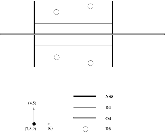
FIG. 19.: Fourbranes stretched between $NS5$-branes which are stuck on an $O4$-plane in the presence of $D6$-branes provide an alternative description of $N=2$ SYM with orthogonal and symplectic gauge groups.

One way to study what happens when an $NS5$-brane intersects an $O4$-plane is to start with a pair of such fivebranes (i.e. a fivebrane and its mirror image) near the orientifold in $(x^{7},x^{8},x^{9})$, and study the transition in which the pair approaches each other and the orientifold, and then splits along the orientifold (in $x^{6}$). This process is described in Fig. 20.

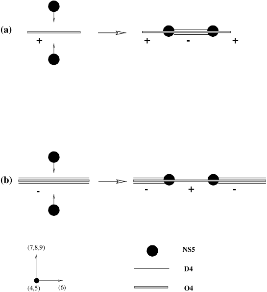
FIG. 20.: (a) An $NS5$-brane and its mirror image approach an $O4_{+}$ plane and separate along it (in $x^{6}$). The portion of the orientifold between the fivebranes flips sign in the process, and a pair of $D4$-branes stretch between the fivebranes. (b) When an $NS5$-brane and its image approach an $O4_{-}$ plane with two adjacent $D4$-branes, the reverse of (a) happens.

A closer look reveals that when the charge of the orientifold is negative, it is in fact impossible to separate the two $NS5$-branes along the orientifold. The low energy worldvolume theory on a pair of $NS5$-branes near an $O4_{-}$ plane (more precisely on the $1+3$ dimensional spacetime $(x^{0},x^{1},x^{2},x^{3})$) has gauge group $Sp(1)$, and the displacement of the fivebranes in the $x^{6}$ direction is described by an antisymmetric tensor of $Sp(1)$, i.e. a singlet. Since it is impossible to Higgs $Sp(1)$ using a singlet, it is impossible to separate the two $NS5$-branes on the $O4_{-}$ plane.

For positive orientifold charge the separation of Fig. 20(a) is attainable. $NS5$-branes near an $O4_{+}$ plane are described by an $SO(2)$ gauge theory. The motions in the $x^{6}$ direction are described by a symmetric tensor of $SO(2)$, which includes a pair of charged scalars. Giving an expectation value to the symmetric tensor completely breaks the $SO(2)$ symmetry and corresponds to displacing the two fivebranes relative to each other on the $O4_{+}$ plane.

What happens when an $NS5$-brane and its image approach an $O4_{+}$ plane and, after getting stuck on it, separate in the $x^{6}$ direction? Each of the fivebranes divides the orientifold into two disconnected parts. One can show that the parts of the orientifold on different sides of the fivebrane must carry opposite RR charge. This has been first shown by [92] by comparing to gauge theory (see below); a worldsheet explanation of this effect was given in [90]. Since far from the fivebranes the orientifold charge must (by locality) be positive, between the fivebranes it is negative. Furthermore, the total RR charge must be continuous across each fivebrane, since otherwise the net charge would curve the fivebrane according to (61) and, in particular, change its shape at infinity, again violating locality. Therefore, one expects to find two $D4$-branes stretched between the fivebranes.

Similarly, when a pair of $NS5$-branes approaches a negatively charged $O4$-plane with two $D4$-branes embedded in it, it can split into two fivebranes at different values of $x^{6}$, and gives rise to the configuration depicted in Fig. 20(b). Both possibilities are useful for describing gauge theories using branes.

Once we understand the behavior of $NS5$-branes near $O4$-planes, that of $D6$-branes is in principle determined by U-duality. In particular, it appears that bringing pairs of $D6$-branes close to an $O4_{+}$ plane and separating them in $x^{6}$ splits the orientifold into components with alternating positive and negative charges. This might at first sight seem surprising, but it is related by U-duality to the behavior of $NS5$-branes intersecting $O4$-planes. Compactifying $x^{3}$ one can use T-duality to map a $D6$-brane intersecting an $O4$-plane to a $D5$-brane stretched in $(x^{0},x^{1},x^{2},x^{7},x^{8},x^{9})$ intersecting an $O3$-plane stretched in $(x^{0},x^{1},x^{2},x^{6})$ and again cutting it into two disconnected pieces. This system can be analyzed by using S-duality, and properties of $NS5$-branes.

Indeed, if we replace the $D5$-brane by an $NS5$-brane, we arrive at a system similar to that of Fig. 20, with the $O4$-plane replaced by an $O3$-plane. The three dimensional analog of the transition described in that figure is the following: a pair of $NS5$-branes approach an $O3_{+}$ plane, and separate in $x^{6}$ on it. The segment of the $O3$-plane between the fivebranes flips sign and there is a single $D3$-brane embedded in it to make the total RR charge continuous.

S-duality applied to this configuration gives rise (using the results of section III) to a configuration with two $D5$-branes intersecting an $O3$-plane and dividing it into three segments. The leftmost and rightmost parts of the orientifold have negative charge and a $D3$-brane embedded in them, while the segment between the $D5$-branes has positive RR charge. Thus we conclude that the RR charge of the $O3$-plane jumps as we cross a $D5$-brane. Since the statement is true for any finite radius of $x^{3}$, $R$, it is also true as $R\to\infty$. Therefore, we conclude that the RR charge of the $O4$-plane jumps as it crosses a $D6$-brane.

We will also need to understand the generalization of the s-rule to $D4$-branes stretched between an $NS5$-brane and a $D6$-brane both of which are stuck on an $O4$-plane. A natural guess is the following. The usual s-rule forbids configurations where two or more $D4$-branes are forced to be right on top of each other. In the presence of an $O4$-plane, it is natural to expect that if a part of the $O4$-plane between an $NS5$-brane and a $D6$-brane has negative charge and no $D4$-branes, one can connect the two branes by a pair of $D4$-branes. If the part of the orientifold between the two branes has positive charge, or negative charge with two $D4$-branes embedded in it (or any combination of these), one cannot stretch any further fourbranes between them.

We are now finally ready to turn to applications. When the charge of the segment of the orientifold between the fivebranes is negative, the brane configuration of Fig. 19 describes an $SO(N_{c})$ gauge theory (we assume that $N_{c}$ is even for now). To describe matter we add $D6$-branes. Note that when all the $D4$-branes are stretched between the $NS5$-branes (in the Coulomb branch), the $D6$-branes sit in pairs that cannot be separated further, as discussed above. The number of $D6$-branes must be even; we took it to be $2N_{f}$, which corresponds to $N_{f}$ hypermultiplets in the $({\bf N_{c}})$ of $SO(N_{c})$. The $N_{c}/2$ dimensional Coulomb branch is described as usual by displacing the $D4$-branes along the $NS5$-branes in pairs away from the orientifold plane. The Higgs branch is obtained by studying all possible breakings of the $D4$-branes on $D6$-branes. Taking into account the s-rule in the presence of an $O4$-plane explained above leads to the splitting pattern of Fig. 21(a).

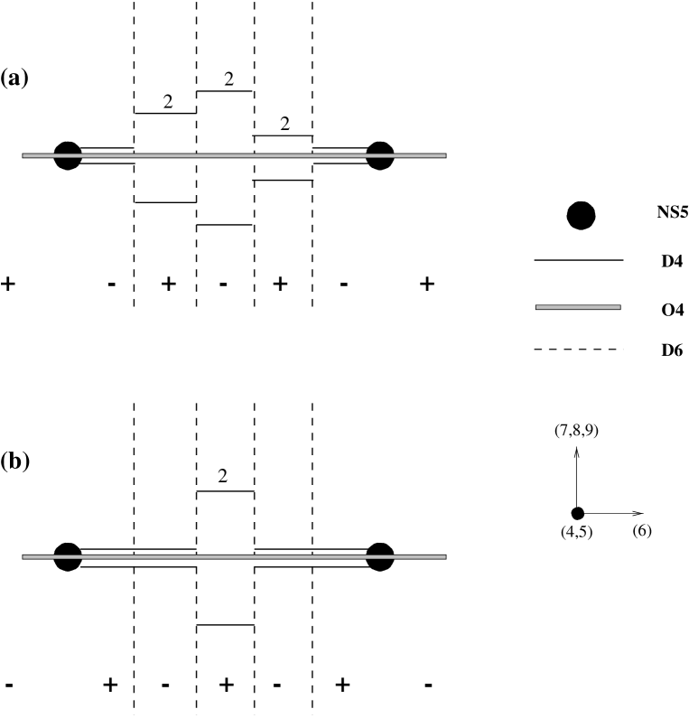
FIG. 21.: The fully Higgsed branches of $N=2$ SYM with (a) $G=SO(2)$ and $N_{f}=2$ charged hypermultiplets; (b) $G=Sp(1)$ and $N_{f}=2$ fundamental hypermultiplets. The orientifold charge flips sign, as indicated at the bottom, whenever one crosses a $D6$ or $NS5$-brane.

The resulting dimension of the fully Higgsed branch (for $N_{f}>N_{c}$) is

$${\rm dim}{\cal M}_{H}=2\sum_{i=1}^{N_{c}\over 2}\left[2N_{f}-(4i-3)\right]=2N_{f}N_{c}-N_{c}(N_{c}-1)$$ (114)

in agreement with the gauge theory analysis. It is instructive to verify that one also gets the correct pattern of breaking and vacuum structure for low numbers of flavors where the gauge group cannot be completely Higgsed. We leave this as an exercise to the reader. One outcome of this exercise is a description of the case of odd $N_{c}$, which can be obtained from even $N_{c}$ by Higgsing one hypermultiplet and breaking $SO(N_{c})\to SO(N_{c}-1)$.

$Sp(N_{c}/2)$ gauge theory with $N_{f}$ fundamental hypermultiplets is described by the configuration of Fig. 19 with positive RR charge between the fivebranes and negative outside. The charge reversal changes the counting (114) in precisely the right way to reproduce the appropriate gauge theory results. We illustrate the structure of the fully Higgsed branch in Fig. 21(b).

3 Some Generalizations

Once the physics of the basic brane constructions has been understood one can generalize them in many different directions. One obvious example is to increase the number of $NS5$-branes. Consider, for example, a chain of $n+1$ fivebranes labeled from $0$ to $n$, with the $(\alpha-1)$’st and $\alpha$’th fivebrane connected by $k_{\alpha}$ $D4$-branes. In addition, let $d_{\alpha}$ $D6$-branes be localized at points between the $(\alpha-1)$’st and $\alpha$’th $NS5$-branes (see Fig. 22 for an example).

The gauge group is in this case $G=\prod_{\alpha=1}^{n}U(k_{\alpha})$. The matter hypermultiplets are the following: $4-4$ strings connecting the $k_{\alpha}$ fourbranes in the $\alpha$’th interval to the $k_{\alpha+1}$ fourbranes in the $(\alpha+1)$’st interval $(\alpha=1,\cdots,n-1)$ give rise to (bifundamental) hypermultiplets transforming in the $(k_{\alpha},\bar{k}_{\alpha+1})$ of $U(k_{\alpha})\times U(k_{\alpha+1})$. In addition we have $d_{\beta}$ hypermultiplets in the fundamental representation of $U(k_{\beta})$ $(\beta=1,\cdots,n)$. We leave the analysis of the moduli space of vacua and the space of deformations to the reader.

If we add to the previous configuration an orientifold fourplane the gauge group becomes an alternating $SO/Sp$ one. For example, for even $n$ (an odd number of $NS5$-branes) and negative RR charge of the segment of the $O4$-plane between the first and second $NS5$-brane, the gauge group is $G=SO(k_{1})\times Sp(k_{2}/2)\times SO(k_{3})\times\cdots\times Sp(k_{n}/2)$ with bifundamental matter charged under adjacent factors of the gauge group.

FIG. 22.: A theory with a product gauge group and matter in the bifundamental of adjacent factors of the gauge group (as well as fundamental matter of individual factors).

Brane configurations corresponding to theories with such product gauge groups were considered in [52, 219, 160, 110, 91].

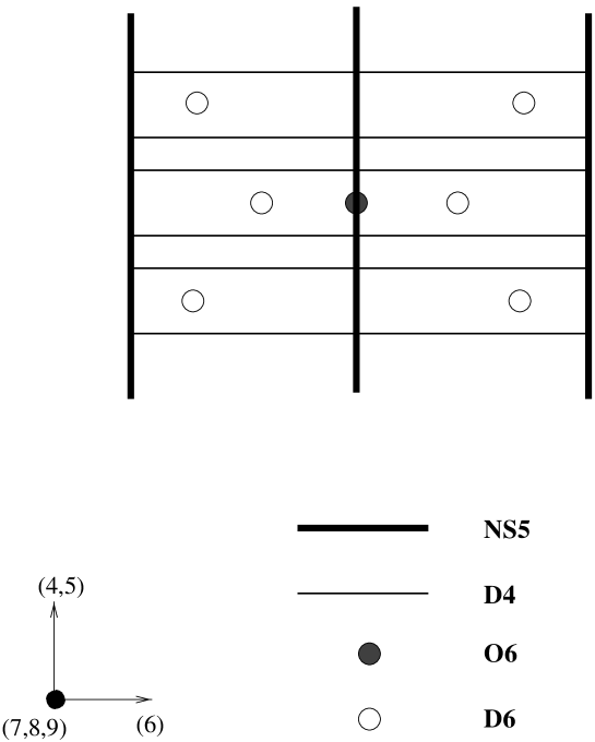
FIG. 23.: A theory with $G=U(N_{c})$ ($N_{c}=6$ in this case), one hypermultiplet in the (anti-) symmetric representation and $N_{f}=3$ fundamentals.

Another example is a generalization of the configuration involving an orientifold sixplane that we discussed previously in the context of orthogonal and symplectic gauge groups. Consider a configuration in which one $NS5$-brane is placed at a distance $L_{6}$ from the $O6$-plane as before, and another $NS5$-brane is placed so that it intersects the orientifold plane. $N_{c}$ $D4$-branes are stretched between the two fivebranes and $N_{f}$ $D6$-branes parallel to the $O6$-plane are placed between the two $NS5$-branes (Fig. 23).

The gauge theory describing this configuration has $G=U(N_{c})$ and a matter hypermultiplet $Z$ in the symmetric or antisymmetric representation of $G$ (depending on the sign of the orientifold), as well as the usual $N_{f}$ fundamental hypermultiplets [159]. The two-index tensor hypermultiplet corresponds to $4-4$ strings stretched from one side of the orientifold to the other side, across the stuck $NS5$-brane.

4 Quantum Effects: I

So far in this section we have described the classical brane configurations and the corresponding classical gauge theory dynamics. For finite $g$ (107) there are important qualitative new effects, which are the subject of this subsection.

We will first discuss these effects in the context of $U(N_{c})$ gauge theory, following [237], which was shown earlier to be described by a system of two $NS5$-branes in type IIA string theory with $N_{c}$ $D4$-branes stretched between them (see Fig. 9). In the next subsection we will comment on the generalization to some of the other cases mentioned above.

For finite $g_{s}$, the type IIA string theory becomes eleven dimensional at short distances. The radius of the eleventh dimension $x^{10}$ is proportional to $g_{s}$, $R_{10}=l_{s}g_{s}$ (38). Furthermore, as we saw in section II C, the $D4$-brane can be thought of as an M-theory fivebrane wrapped around $x^{10}$. Thus, $D4$-branes stretched between $NS5$-branes are reinterpreted in M-theory on $R^{10}\times S^{1}$ as describing a single fivebrane with a curved worldvolume. Since all IIA branes are extended in the $1+3$ dimensions $(x^{0},x^{1},x^{2},x^{3})$ and are located at a point in $(x^{7},x^{8},x^{9})$, the worldvolume of the M-theory fivebrane is $R^{1,3}\times\Sigma$ where $\Sigma$ is a two dimensional surface embedded in the four dimensional space $Q=R^{3}\times S^{1}$ labeled by $(x^{4},x^{5},x^{6},x^{10})$.

It is convenient to parametrize the space $Q$ using the natural complex coordinates

$$s= x^{6}+ix^{10}$$ (115)

$$v= x^{4}+ix^{5}$$ (116)

In the classical type IIA string limit, the $NS5$-branes of (105) are described by $s=$ constant, while the $D4$-branes correspond to $v=$ constant. If we place the two $NS5$-branes at $s=s_{1},s_{2}$ and the $N_{c}$ fourbranes stretched between them at $v=v_{1},v_{2},\cdots,v_{N_{c}}$, the “classical” surface $\Sigma_{cl}$ is described by $(s-s_{1})(s-s_{2})\prod_{a=1}^{N_{c}}(v-v_{a})=0$, with ${\rm Re}(s_{1})\leq{\rm Re}(s)\leq{\rm Re}(s_{2})$. $\Sigma_{cl}$ is a singular surface with different components which meet at the singular points $s=s_{i}$, $v=v_{a}$ ($i=1,2$; $a=1,\cdots,N_{c}$).

As we will see shortly, for finite $R_{10}$ and at generic points in moduli space the singularities in $\Sigma$ are eliminated. To determine the shape of the smooth surface $\Sigma$ we next consider its large $v$ asymptotics. Classically we see at large $v$ the two $NS5$-branes at fixed $s=s_{1},s_{2}$. However, we know from the discussion of subsection II E 3 that the ends of the fourbranes on the fivebrane look like charges . More precisely, $q_{L}$ fourbranes ending on the fivebrane from the left at $v=a_{1},\cdots,a_{q_{L}}$, and $q_{R}$ fourbranes ending on if from the right at $v=b_{1},\cdots,b_{q_{R}}$ curve it asymptotically according to (61) which in this case is:

$$x^{6}=l_{s}g_{s}\sum_{i=1}^{q_{L}}\log|v-a_{i}|-l_{s}g_{s}\sum_{i=1}^{q_{R}}\log|v-b_{i}|$$ (117)

The fact that the coefficient of the $\log$ is proportional to $g_{s}$ can be understood at weak coupling as a consequence of properties of the $NS5$-brane. Equations (19, 27) imply that the SYM coupling of the theory on the fivebrane (reduced to $2+1$ dimensions) has no $g_{s}$ dependence, while the kinetic term of $X^{6}$ is proportional to $1/g_{s}^{2}$. Thus, the BPS saturated solution describing a fourbrane ending on the fivebrane has gauge field $A\simeq Q\log|v|$ with the charge quantum $Q$ independent of $g_{s}$, and $X^{6}\simeq Qg_{s}\log|v|$. The factor of $l_{s}$ in (117) is required by dimensional analysis.

At strong coupling (117) can be alternatively derived by identifying $l_{s}g_{s}$ with $R_{10}$, the only scale in the problem. The weak and strong coupling arguments must agree because the BPS property of the state in question allows one to freely interpolate holomorphic properties between the weak and strong coupling regimes (and, as we will see, (117) is closely related to a holomorphic quantity).

Note that the fact that the end of a fourbrane on a fivebrane looks like a codimension two charged object implies that unlike the case $p>2$ in (61) one cannot, in general, define quantum mechanically “the location of the $NS5$-brane” by measuring $x^{6}$ at $|v|\to\infty$, since the effects of the fourbranes (117) are not small for large $v$. $x^{6}$ approaches a well defined value, which can then be interpreted as the location of the fivebrane, only when the total charge on the fivebrane vanishes, $q_{L}=q_{R}$.

The scalar field $x^{6}$ is related by $N=2$ SUSY to $x^{10}$; together the two form a complex scalar field $s$ (116) that belongs to the vector multiplet of $N=2$ SUSY in the $3+1$ dimensional spacetime. For consistency with SUSY, (117) must be generalized to a holomorphic equation for $s$ (116),

$$s=R_{10}\sum_{i=1}^{q_{L}}\log(v-a_{i})-R_{10}\sum_{i=1}^{q_{R}}\log(v-b_{i})$$ (118)

The real part of this equation is (117); the imaginary part implies that $x^{10}$ jumps by $\pm 2\pi R_{10}$ when we circle $a_{i}$ or $b_{i}$ in the complex $v$ plane. Thus, the ends of fourbranes on the fivebranes look like vortices. Since $x^{10}$ is compact, it will be convenient for later purposes to define

$$t=\exp(-{s\over R_{10}})$$ (119)

in terms of which (118) takes the form

$$t={\prod_{i=1}^{q_{R}}(v-b_{i})\over\prod_{j=1}^{q_{L}}(v-a_{j})}$$ (120)

We are now ready to determine the full shape of the surface $\Sigma$ and thus the embedding of the fivebrane corresponding to the classical brane configuration realizing pure $N=2$ SYM (Fig. 9) in the eleven dimensional spacetime. SUSY requires $\Sigma$ to be given by a holomorphic curve in the two complex dimensional space labeled by $t,v$. It can be described by a holomorphic equation $F(t,v)=0$ for some function $F$. Viewed as a function of $t$ for large $v$ we expect to see two branches corresponding to the two “$NS5$-branes” at (120): $t_{1}\simeq v^{N_{c}}$ and $t_{2}\simeq v^{-N_{c}}$. Therefore, the curve should be described by setting to zero a second order polynomial in $t$,

$$F(t,v)=A(v)t^{2}+B(v)t+C(v)=0$$ (121)

where $A$, $B$ and $C$ are polynomials of degree $N_{c}$ in $v$, so that for fixed $t$ there will be $N_{c}$ solutions for $v$ corresponding to the “$D4$-branes” stretched between the fivebranes.

As we approach a zero of $C(v)$, a solution of the quadratic equation (121) goes to $t=0$, i.e. (119) $x^{6}=\infty$. Thus zeroes of $C(v)$ correspond to locations of semi-infinite fourbranes stretching to the right of the rightmost $NS5$-brane. Similarly, $A(v)$ describes semi-infinite fourbranes stretching to $x^{6}=-\infty$ from the left $NS5$-brane. In the $N=2$ gauge theory application semi-infinite fourbranes give rise to fundamental matter and as a first step we are not interested in them. Thus we set 

$$A(v)=C(v)=1$$ (122)

$B(v)$ is taken to be the most general polynomial of degree $N_{c}$ which can, by rescaling and shifting $v$, be brought to the form

$$B(v)=v^{N_{c}}+u_{2}v^{N_{c}-2}+u_{3}v^{N_{c}-3}\cdots+u_{N_{c}}$$ (123)

$u_{2},\cdots,u_{N_{c}}$ are complex constants parametrizing the polynomial $B$. The curve (121) with the choice (122, 123) of $A$, $B$ and $C$ has the right structure: for fixed $t$ it has $N_{c}$ roots $v_{i}$ corresponding to the $N_{c}$ “fourbranes.” Note that while classically there should only be such solutions for $t$ between the $NS5$-branes, because of the bending (120) there are in fact $N_{c}$ solutions for $v$ for any $t\not=0$. Similarly, for all $v$ there are two solutions for $t$, which for large $v$ behave like

$$t_{\pm}\simeq v^{\pm N_{c}}$$ (124)

in agreement with the general structure expected from (120).

To recapitulate, just like classically there is a one to one correspondence between configurations of $D4$-branes stretched between $NS5$-branes and vacua of classical $N=2$ SYM, quantum mechanically there is a one to one correspondence between vacua of quantum $N=2$ SYM and supersymmetric configurations of an $M5$-brane with worldvolume $R^{3,1}\times\Sigma$, with $\Sigma$ described by (121-123). Roots of the polynomial $B$ (123) correspond to “the locations of the $D4$-branes” and label different points in the quantum Coulomb branch of the $N=2$ SYM theory.

It is interesting that there are only $N_{c}-1$ independent roots, labeled by the moduli $\{u_{i}\}$. This appears to be in contradiction with the fact that there are $N_{c}$ massless vectormultiplets living on the fourbranes for generic values of the moduli $\{u_{i}\}$ corresponding to the unbroken $U(1)^{N_{c}}\subset U(N_{c})$. In fact, the number of vectormultiplets is $N_{c}-1$, in agreement with (123). The $U(1)\subset U(N_{c})$ has vanishing coupling and is “frozen.”

This can be understood semiclassically by evaluating the kinetic term of the $U(1)$. The $N_{c}$ “fourbranes” ending on an $NS5$-brane from the left (say), bend it according to (118). $a_{i}$ are the moduli, and to probe their dynamics one should allow them to slowly vary as a function of $(x^{0},x^{1},x^{2},x^{3})$. The kinetic energy of the fivebrane behaves for such slowly varying configurations as

$$S\simeq\int d^{4}x\int d^{2}v|\partial_{\mu}s|^{2}\simeq R_{10}^{2}\int d^{4}x\int d^{2}v|\sum_{i}\partial_{\mu}a_{i}{1\over v-a_{i}}|^{2}$$ (125)

At large $v$, where (125) is expected to be accurate, we find

$$S\simeq R_{10}^{2}\int{d^{2}v\over|v|^{2}}\int d^{4}x|\sum_{i}\partial_{\mu}a_{i}|^{2}$$ (126)

The logarithmically divergent $v$ integral (126) leads to a vanishing coupling for the $U(1)\subset U(N_{c})$

$${1\over g_{1}^{2}}\simeq R_{10}^{2}\int{d^{2}v\over|v|^{2}}\to\infty$$ (127)

Interestingly, equations (121-123) describe the Seiberg-Witten curve for $SU(N_{c})$ gauge theory with no matter! In gauge theory, the low energy coupling matrix $\tau_{ij}$ (90) is the period matrix of the corresponding Riemann surface. This is also the case in the fivebrane construction. The worldvolume theory of a flat fivebrane includes a self-dual $B_{\mu\nu}$ field $(H=dB=*dB)$. Upon compactification on $\Sigma$, $B$ gives rise to $g$ abelian vectormultiplets in $3+1$ dimensions, with $g$ the genus of the Riemann surface $\Sigma$. In our case, the surface $\Sigma$ can be thought of as describing two sheets (the “fivebranes”) connected by $N_{c}$ tubes (the “fourbranes”), and hence it has genus $g=N_{c}-1$. The coupling matrix of the resulting $U(1)^{N_{c}-1}$ gauge theory is the period matrix of $\Sigma$ [229].

Another derivation of the relation between the period matrix of the Riemann surface around which the fivebrane is wrapped and the coupling matrix of the abelian gauge theory on the brane that emphasizes the role of the scalar fields living on the brane appears in [134].

To summarize, the brane analysis agrees with SW theory. It offers a rationale as to why the low energy gauge coupling matrix and metric on moduli space of $N=2$ SYM are described by a period matrix of a Riemann surface. The natural context for studying SW theory appears to be as a compactification of the $(2,0)$ field theory of an $M5$-brane (the low energy limit of the theory of $M5$ or type IIA $NS5$-branes) on the Riemann surface $\Sigma$.

At this point we would like to pause for a few comments on the foregoing discussion:

1. Global Symmetry, Conformal Invariance And The Shape Of The Fivebrane

As we discussed in section IV A, classical $N=2$ SYM has at the origin of moduli space a global symmetry $SU(2)_{R}\times U(1)_{R}$. The $SU(2)_{R}$ symmetry is part of $N=2$ SUSY; the $U(1)_{R}$ reflects the classical conformal invariance of the theory and is broken at one loop by the chiral anomaly to $Z_{2N_{c}}$.

In the brane description, the $U(1)_{R}$ symmetry is realized as the $SO(2)$ rotation group of the $v$ plane, which acts as $v\to v\exp(i\alpha)$. The classical configuration of $N_{c}$ $D4$-branes – all at $v=0$ – stretched between the two $NS5$-branes (say, at $s=0$) is invariant under this $SO(2)$ symmetry. The brane analog of one loop effects is the leading quantum correction, which is the asymptotic bending (118). It breaks the $U(1)_{R}$ symmetry by curving the left and right fivebranes  to

$$s_{L}= -N_{c}R_{10}\log v$$ (128)

$$s_{R}= +N_{c}R_{10}\log v$$ (129)

This configuration is no longer invariant under

$$v\to v\exp(i\alpha)$$ (130)

Under (130)

$$s_{L}\to s_{L}-N_{c}R_{10}i\alpha$$ (131)

$$s_{R}\to s_{R}+N_{c}R_{10}i\alpha$$ (132)

For generic $\alpha$ (132) is clearly not a symmetry, however, there are residual discrete symmetry transformations corresponding to $\alpha=2\pi n/2N_{c}$ due to the fact that ${\rm Im}s=x^{10}$ lives on a circle of radius $R_{10}$. Thus a $Z_{2N_{c}}$ subgroup of $U(1)_{R}$ remains unbroken, in agreement with the gauge theory analysis.

2. Adding Flavors

It is easy to add fundamental hypermultiplets to the discussion. As we have noted above, to describe the Coulomb branch of a model with $N_{f}$ fundamentals of $SU(N_{c})$ we can add $N_{f}$ semi-infinite fourbranes, say to the right of the $NS5$-branes. These are described by turning on $C(v)$ in (121):

$$C(v)=\prod_{i=1}^{N_{f}}(v-m_{i})$$ (133)

$m_{i}$ are the locations of the semi-infinite fourbranes in the $v$ plane which, as we have seen, correspond to the masses of the fundamental “quarks.” Thus $N=2$ SQCD with $G=SU(N_{c})$ and $N_{f}$ fundamentals is described by the Riemann surface

$$t^{2}+B(v)t+C(v)=0$$ (134)

with $B(v)$ given by (123) and $C(v)$ by (133). This agrees with the gauge theory results of [121, 27].

3. ${\bf SU(N_{c})}$ Versus ${\bf U(N_{c})}$

We have argued that the brane configuration of Fig. 9, which classically describes a $U(N_{c})$ gauge theory, in fact corresponds quantum mechanically to an $SU(N_{c})$ one; the coupling of the extra $U(1)$ factor vanishes. This observation appears to be in contradiction with the fact that the moduli and deformations of the brane configuration discussed above seem to be those of a $U(N_{c})$ theory. This issue remains unresolved as of this writing; below we explain the specific puzzles.

We saw previously that the moduli space of brane configurations seems to match the classical Higgs branch of $U(N_{c})$ gauge theory with $N_{f}$ hypermultiplets. If the gauge group is $SU(N_{c})$, the complex dimension of the Higgs branch is $2N_{f}N_{c}-2(N_{c}^{2}-1)$ and the brane counting misses two complex moduli. By itself, this need not be a serious difficulty; we saw previously examples where some or all of the field theory moduli were not seen in the brane analysis. Unfortunately, the mismatch in the structure of the Higgs branch is related to a more serious difficulty having to do with the field theory interpretation of certain deformations of the brane configuration.

In the classical discussion we have interpreted the relative location of the two $NS5$-branes in $(x^{7},x^{8},x^{9})$ as a FI D-term for the $U(1)\subset U(N_{c})$ (112). If the gauge group is $SU(N_{c})$, we have to modify that interpretation, as the theory no longer has a FI coupling. The question is whether in the quantum theory the parameters corresponding to a relative displacement of the two asymptotic parts of the $M5$-brane in $(x^{7},x^{8},x^{9})$ are moduli in the $3+1$ dimensional field theory on the brane, or whether – like the $U(1)$ vectormultiplet – they are decoupled. There seem to be two logical possibilities, each of which has its own difficulties [110].

An argument similar to that outlined in equations (125-127) would suggest that these parameters are frozen and correspond to couplings in the $3+1$ dimensional gauge theory. The kinetic energy of the scalar fields $X^{I}$, $I=7,8,9$, seems to diverge (assuming an asymptotically flat metric on the fivebrane, as we have for $X^{6}(x^{\mu})$, (125)) as

$${\cal L}_{\rm kin}\simeq\int d^{2}v(\partial_{\mu}X^{I})^{2}$$ (135)

Thus, the kinetic energy of the fields $X^{I}$ is infinite and we must find a coupling in the Lagrangian of $SU(N_{c})$ gauge theory that has the same effect on the vacuum structure as a FI D-term (112). It is not known (to us) how to write such a coupling. In order for such a coupling to exist, the $U(1)$ factor would have to be unfrozen, and the estimate of the kinetic energy (125-127) would have to be invalid.

Alternatively, one might imagine that the parameters corresponding to $(x^{7},x^{8},x^{9})$ are in fact moduli in the gauge theory. This would apparently be consistent with gauge theory; these moduli would provide three of the four missing moduli parametrizing the baryonic branch of the theory. However, for this interpretation to be valid we have to come up with a mechanism for rendering the naively divergent kinetic energy (135) finite (without spoiling (125)). This sounds even more implausible than the first scenario as one has to cancel a more divergent kinetic energy. It is not clear to us what is the resolution of this problem.

4. ${\bf N_{f}\geq 2N_{c}}$

For $N_{f}=2N_{c}$, at the origin of the Coulomb branch and for vanishing quark masses, the curve (134) is:

$$t^{2}+av^{N_{c}}t+bv^{2N_{c}}=0$$ (136)

or equivalently

$$t_{\pm}=\lambda_{\pm}v^{N_{c}}$$ (137)

with $\lambda_{\pm}$ the two solutions of

$$\lambda^{2}+a\lambda+b=0$$ (138)

The $U(1)_{R}$ symmetry

$$v\to e^{i\alpha}v$$ (139)

$$t\to e^{iN_{c}\alpha}t$$ (140)

is unbroken. Thus the theory at the origin is an interacting non-trivial $N=2$ SCFT. This is consistent with the fact that the curve (137) is singular at $t=v=0$ – a hallmark of a non-trivial SCFT. The ratio $w=\lambda_{+}\lambda_{-}/(\lambda_{+}-\lambda_{-})^{2}$ is invariant under rescaling of $t$, $v$ and can be thought of as parametrizing the coupling constant of the SCFT. For weak coupling, $w\simeq 0$, one has $w=\exp(2\pi i\tau)$ ($\tau$ is the complex gauge coupling), but more generally, due to duality, $\tau$ is a many valued function of $w$.

For $N_{f}>2N_{c}$ the description (134) seems to break down. Both solutions for $t$ behave at large $v$ as $t\sim v^{N_{f}/2}$, while (118) (in the presence of $N_{f}$ semi-infinite “fourbranes” stretching to $x^{6}\to\infty$) predicts $t_{1}\sim v^{N_{c}}$, $t_{2}\sim v^{N_{f}-N_{c}}$. Not coincidentally, in this case the gauge theory is not asymptotically free and must be embedded in a bigger theory to make it well defined in the UV. And, in any case, it is free in the IR. It is in fact possible to modify (134) to accommodate these cases (see [237] for details).

5. BPS States

The fivebrane description of $N=2$ SYM can also be used to study massive BPS saturated states. Examples of such states in SYM include charged gauge boson vectormultiplets and magnetic monopole hypermultiplets. In the classical IIA limit, massive gauge bosons are described by fundamental strings stretched between different fourbranes. For finite $R_{10}$ these fundamental strings are reinterpreted as membranes wrapped around $x^{10}$. Thus, charged $W$ bosons are described in M-theory by minimal area membranes ending on the fivebrane. Clearly, the topology of the resulting membrane is cylindrical.

Monopoles are described in the IIA limit by $D2$-branes stretched between the two $NS5$-branes and two adjacent $D4$-branes, as in Fig. 8. In M-theory they correspond to membranes with the topology of a disk ending on the fivebrane.

There are other BPS states such as quarks and various dyons, all of which are described in M-theory by membranes ending on the fivebrane. Membranes with the topology of a cylinder always seem to give rise to vectormultiplets, while those with the topology of a disk give hypermultiplets. We will not describe the corresponding membranes in detail here, referring instead to [129, 168].

6. Compact Coulomb Branches And Finite ${\bf N=2}$ Models

The fact that the gauge coupling of the $U(1)\subset U(N_{c})$ vanishes is related to the infinite area of the $v$-plane (127). One might wonder what would happen if we compactified $(x^{4},x^{5})$ on a two-torus.

Already classically we see that in this situation the Coulomb branch of the theory, labeled by locations of $D4$-branes stretched between fivebranes, becomes compact. Quantum mechanically we see that since (118) is a solution of a two dimensional Laplace equation

$$\partial_{v}\partial_{\bar{v}}s=R_{10}\sum_{i=1}^{q_{L}}\delta^{2}(v-a_{i})-R_{10}\sum_{i=1}^{q_{R}}\delta^{2}(v-b_{i})$$ (141)

on a compact surface, the total charge on each fivebrane must vanish: $q_{L}=q_{R}$. This means that there must be $N_{c}$ semi-infinite fourbranes attached to each fivebrane and the total number of flavors must thus be $N_{f}=2N_{c}$. The solution of (141) that generalizes (118) to the case of a two-torus is ($q=q_{L}=q_{R}$):

$$s=R_{10}\sum_{i=1}^{q}\left[\log\chi(v-a_{i}|\rho)-\log\chi(v-b_{i}|\rho)\right]$$ (142)

where $\rho$ is the modular parameter (complex structure) of the $v$-plane torus ($v\sim v+1$, $v\sim v+\rho$), and

$$\chi(z|\rho)={\theta_{1}(z|\rho)\over\theta^{\prime}_{1}(0|\rho)}$$ (143)

$\log\chi$ is related to the propagator of a two dimensional scalar field on a torus with modulus $\rho$ (see [117] for notation and references). Note that $\chi$ itself is not well defined on the torus; its periodicity properties are:

$$\chi(z+1|\rho)=-\chi(z|\rho)$$ (144)

$$\chi(z+\rho|\rho)=-e^{-i\pi\rho-2i\pi z}\chi(z|\rho)$$ (145)

However, we only require that the curve built using $\chi$ should exhibit the periodicity. To construct this curve, start with the infinite volume curve (121) describing this situation 

$$t^{2}\prod_{i=1}^{N_{c}}(v-m_{i}^{(1)})+t\prod_{i=1}^{N_{c}}(v-v_{i})+\prod_{i=1}^{N_{c}}(v-m_{i}^{(2)})=0$$ (146)

and replace each $(v-a_{i})$ by $\chi(v-a_{i}|\rho)$. This gives

$$t^{2}\prod_{i=1}^{N_{c}}\chi(v-m_{i}^{(1)}|\rho)+t\prod_{i=1}^{N_{c}}\chi(v-v_{i}|\rho)+\prod_{i=1}^{N_{c}}\chi(v-m_{i}^{(2)}|\rho)=0$$ (147)

Using (145) and the fact that the moduli $v_{i}$ and masses $m_{i}$ satisfy the relations

$$\sum_{i=1}^{N_{c}}(v_{i}-m_{i}^{(1)})={\rm const}$$ (148)

$$\sum_{i=1}^{N_{c}}(v_{i}-m_{i}^{(2)})={\rm const}$$ (149)

we find that the curve (147) indeed has the right periodicity properties.

At first sight the generalization of $N=2$ SYM with compact Coulomb branch seems mysterious, but in fact it can be thought of as the moduli space of vacua of a six dimensional “gauge theory” compactified on a two-torus. Indeed, if $v$ parametrizes a two-torus $T^{2}$, we can T-dualize our classical configuration of $D4$-branes ending on $NS5$-branes, and using the results of section II reach a configuration of $D6$-branes wrapped around the dual torus $\tilde{T}^{2}$ and ending on the $NS5$-branes in the $x^{6}$ direction.

From the six dimensional point of view it is clear that we must require $N_{f}=2N_{c}$, since the only configuration consistent with RR charge conservation involves in this case $N_{c}$ infinite $D6$-branes extending to infinity in $x^{6}$ and intersecting the two $NS5$-branes. Wilson lines around the $\tilde{T}^{2}$ give rise to the parameters $m$, $v$ (147). From the gauge theory point of view, $N_{f}=2N_{c}$ is necessary due to the requirement of cancellation of six dimensional chiral anomalies.

The curve (147) exhibits an $SL(2,Z)$ duality symmetry corresponding to modular transformations $\rho\to(a\rho+b)/(c\rho+d)$ under which

$$\chi\left({z\over c\rho+d}|{a\rho+b\over c\rho+d}\right)={\eta\exp({i\pi cz^{2}\over c\rho+d})\over c\rho+d}\chi(z|\rho)$$ (150)

$\eta$ is an eight-root of unity. This $SL(2,Z)$ symmetry provides a geometric realization of the duality symmetry of finite $N=2$ SYM models (which are anomaly free in $6d$ and thus can be lifted to $6d$). Note that the area of the $v$-plane torus does not appear in (147). This is essentially because $v$ has been rescaled to absorb a factor of the area. The four dimensional limit of (147) is obtained by taking $v\ll 1,\rho$ where $\chi(v|\rho)$ reduces to $v$.

7. SQCD Versus MQCD

As we discussed before, the limit that one needs to take to study decoupled gauge dynamics on the fivebrane is $R_{10},L_{6}\to 0$ holding $R_{10}/L_{6}=g_{SYM}^{2}$ fixed. In this limit the fivebrane becomes singular although its complex structure (134) is regular. To fully understand gauge dynamics in this limit one needs to study the fivebrane theory in the IIA limit.

Witten has suggested to study the theory in the opposite limit $R_{10},L_{6}\to\infty$, $R_{10}/L_{6}$ fixed, observing that in that limit (134) describes a large smooth fivebrane and thus can be accurately studied by using low energy M-theory, i.e. eleven dimensional supergravity (the fivebrane dynamics in this limit is sometimes referred to in the literature as “MQCD”).

For holomorphic properties of the vacuum, such as the low energy gauge couplings and metric on moduli space (89-91), the two limits must agree due to SUSY. However, non-holomorphic low energy features are quite different in the two limits. In particular, in the MQCD limit the fivebrane dynamics is no longer effectively four dimensional, and there is large mixing between gauge degrees of freedom and other excitations. Thus, it is misleading to refer to the M-theory limit as QCD (M or otherwise).

The situation is similar to the well known worldsheet duality in open plus closed string theory. The physics can be viewed either in the open string channel (where light states are typically gauge fields) or as due to closed string exchange (gravitons, dilatons, etc.). Worldsheet duality implies that the two representations must agree, but one may be simpler than the other. In some situations the open string representation is dominated by the massless sector, but then in the closed string channel one needs to sum over exchanges of arbitrarily heavy string states. In such cases, the relevant physics is that of gauge theory.

In other cases, the closed string channel is dominated by exchange of massless modes such as gravitons, but then the open string calculation receives contributions from arbitrarily heavy states and there is no simple gauge theory interpretation of the physics.

The only known cases (with the possible exception of DLCQ matrix theory – reviewed in [32, 47] – whose status is unclear as of this writing) where there is a simple interpretation in both the open and closed string channels involve quantities protected by supersymmetry.

In our case, the analog of the closed string channel is the eleven dimensional “MQCD” limit $R_{10},L_{6}\to\infty$ where physics is dominated by gravity, while the analog of the open string channel is the IIA limit $R_{10},L_{6}\to 0$. Low energy features that are not protected by SUSY need not agree in the two limits (except perhaps in certain large $N$ limits). SQCD corresponds to the latter.

8. Non-Trivial Infrared Fixed Points

At generic points in the Coulomb branch, the infrared dynamics of $N=2$ SYM is described by $r$ massless photons whose coupling matrix is the period matrix of the Riemann surface $\Sigma$. At points where additional matter goes to zero mass, the infrared dynamics changes, and in many cases describes a non-trivial SCFT [24, 26]. These situations correspond to degenerate Riemann surfaces $\Sigma$.

Whenever that happens, the supergravity description breaks down, even if $R_{10}$ and $L_{6}$ are large. Thus, eleven dimensional supergravity provides a useful description of the fivebrane wrapped on $\Sigma$ only sufficiently far from any points in moduli space where the infrared behavior changes; in particular, it cannot be used to study (beyond the BPS sector) the non-trivial SCFTs discussed by [24, 26].

5 Quantum Effects: II

The analysis of the previous subsection can be easily generalized to the chain of fivebranes connected by fourbranes mentioned above [237]. Specifically, consider the IIA configuration of $n+1$ $NS5$-branes labeled by $\alpha=0,1,\cdots,n$, with $k_{\alpha}$ $D4$-branes connecting the $(\alpha-1)$’st and $\alpha$’th fivebranes (Fig. 22). For simplicity, we assume that there are no semi-infinite fourbranes at the edges.

Classically we saw that the gauge group was $\prod_{\alpha=1}^{n}U(k_{\alpha})$, but the $n$ $U(1)$ factors are frozen as before. Thus the gauge group is

$$G=\prod_{\alpha=1}^{n}SU(k_{\alpha})$$ (151)

with matter in the bifundamental representation $(k_{\alpha},\bar{k}_{\alpha+1})$ of adjacent factors of the gauge group. We will further assume that all factors in (151) are asymptotically free:

$$2k_{\alpha}-(k_{\alpha_{+}1}+k_{\alpha-1})\geq 0,\;\;\;\;\;\forall\alpha$$ (152)

Following the logic of our previous discussion we expect the Riemann surface $\Sigma$ to be described in this case by the holomorphic equation

$$F(t,v)=t^{n+1}+P_{k_{1}}(v)t^{n}+P_{k_{2}}(v)t^{n-1}+\cdots+P_{k_{n}}(v)t+1=0$$ (153)

The fact that (153) is a polynomial of degree $n+1$ in $t$ ensures that there are $n+1$ solutions for $t$ corresponding to the $n+1$ $NS5$-branes. The $v$ independence of the coefficients of $t^{n+1}$ and $1$ implies the absence of semi-infinite fourbranes. The degrees of the polynomials in $v$ $P_{k_{\alpha}}=c_{\alpha}v^{k_{\alpha}}+\cdots$ are determined by the fact that rewriting

$$F(t,v)=\prod_{\alpha=0}^{n}(t-t_{\alpha}(v))$$ (154)

the locations of the $n+1$ fivebranes $t_{\alpha}(v)$ must behave for large $v$ as (118-120):

$$t_{\alpha}(v)\sim v^{k_{\alpha+1}-k_{\alpha}}$$ (155)

(where $k_{0}=k_{n+1}=0$); to check that this leads to (153) one has to use (152). The roots of $P_{k_{\alpha}}(v)$ correspond to the positions of the $k_{\alpha}$ fourbranes connecting the $(\alpha-1)$’st and $\alpha$’th fivebranes.

As we have seen in the classical brane construction, semi-infinite fourbranes provide a convenient tool to describe the Coulomb branch of SQCD with fundamental matter, but to study the full moduli space of vacua (in particular, to see the Higgs branches) it is necessary to introduce $D6$-branes. Our next task is to understand models with sixbranes at finite $R_{10}/L_{6}$.

Recall that the $D6$-brane corresponds in M-theory to a KK monopole magnetically charged under $G_{\mu 10}$. The (hyper-Kähler) metric around a collection of KK monopoles is the multi Taub-NUT metric (30-32). We do not actually need the metric around a KK monopole, but only its complex structure. The hyper-Kähler manifold (30-32) in fact admits three independent complex structures, any of which is suitable for our purposes.

The typical situation we will be interested in is one where there are $N_{f}$ KK monopoles at $v=m_{1},\cdots,m_{N_{f}}$. One of the complex structures of the corresponding multi Taub-NUT space can be described by embedding it in a three complex dimensional space with coordinates $y,z,v$. It is given by:

$$yz=\prod_{i=1}^{N_{f}}(v-m_{i})$$ (156)

When all the KK monopoles coincide, (156) approaches an $A_{N_{f}-1}$ singularity $yz=v^{N_{f}}$. The symmetry $y\to\lambda y$, $z\to\lambda^{-1}z$ of (156) corresponds to $t\to\lambda t$. Thus one can think of $y$ as corresponding to $t$ (with $z$ fixed) or of $z$ as corresponding to $t^{-1}$ (with $y$ fixed).

Note that the complex structure (156) is insensitive to the $x^{6}$ location of the $N_{f}$ KK monopoles. That information resides in the Kähler class of the metric (30-32) which does depend on $x^{6}$. Thus even when different $m_{i}$ in (156) coincide, the corresponding $A_{N_{f}-1}$ singularity may still be resolved by separating the centers of the monopoles in $x^{6}$.

Consider as an example $N=2$ SQCD with gauge group $G=SU(N_{c})$ and $N_{f}$ flavors, realized classically as $N_{f}$ $D6$-branes situated between the two $NS5$-branes in the $x^{6}$ direction (Fig. 14). At finite $L_{6}/R_{10}$ we need again to find the shape of an $M5$-brane, except now it lives not in $Q=R^{3}\times S^{1}$, but rather in $\tilde{Q}=$ resolved $A_{N_{f}-1}$ multi Taub-NUT space (156).

We can again describe the fivebrane by a curve of the form

$$A(v)y^{2}+B(v)y+C(v)=0$$ (157)

with some polynomials $A$, $B$, $C$. As before, $A(v)=1$, since otherwise $y$ (and, therefore, $t$) diverges at roots of $A(v)$. Rewriting (157) in terms of $z=\prod(v-m_{i})/y$ and requiring that there should be no singularities of $z$ for finite $v$ (these too would correspond to semi-infinite fourbranes) one finds that $C=a\prod(v-m_{i})$ (see [237] for a more detailed analysis). Finally, $B(v)$ (157) is a polynomial of degree $N_{c}$ as before (123).

Thus we recover the solution found before using semi-infinite fourbranes. The fact that the result (157) is independent of the $x^{6}$ position of the $D6$-branes is consistent with our discussion in subsection IV C 1 where this was deduced as a consequence of the HW transition.

The description of $N=2$ SQCD with sixbranes (KK monopoles) can be used to describe the Higgs branch of the theory as well. We refer to [237] for a detailed discussion of this.

Finally, $N=2$ gauge theories on $N_{c}$ fourbranes in the presence of sixbranes and orientifold planes can be lifted to M-theory, and used to derive the curves and describe the Higgs branches of $SO(N_{c})$ and $Sp(N_{c}/2)$ theories as well as many product groups [160, 53, 94, 174, 159, 173, 91].

V Four Dimensional Theories With $N=1$ SUSY

In this section we turn our attention to four dimensional $N=1$ supersymmetric gauge theories which typically have the richest dynamics among the different SYM theories and are the closest to phenomenology.

As we saw in the previous sections, $N=4$ supersymmetric gauge theory has the simplest dynamics and phase structure. The theory is specified by the choice of a gauge group; all matter is in the adjoint representation. The vacuum structure consists of a Coulomb branch with singularities corresponding to points of enhanced unbroken gauge symmetry. The most singular point is the origin of moduli space, which corresponds to a non-trivial CFT parametrized by the exactly marginal gauge coupling $g$. The form of the effective action up to two derivatives is completely determined by the symmetry structure; in particular, the metric on the Coulomb branch is flat. The leading terms that receive quantum corrections are certain non-renormalizable (=irrelevant) four derivative terms, and these corrections can be controlled since they receive contributions only from BPS states. The most interesting feature of the dynamics of $N=4$ SYM is the discrete identification of theories on the line of fixed points labeled by $g$ provided by Montonen-Olive duality (which acts as $g\leftrightarrow 1/g$). Another interesting phenomenon is the appearance of non-trivial infrared fixed points of the RG at which electrically and magnetically charged particles become massless at the same time.

In the $N=2$ SYM case there are some new features. Theories are now labeled by the choice of a gauge group and a set of matter representations. Non-trivial quantum corrections to the two derivative terms in the vectormultiplet action lead to a modification of the metric on the Coulomb branch, described by Seiberg and Witten. In addition, Higgs branches in which the rank of the gauge group is reduced appear; as we saw before, $N=2$ theories typically have a rather rich phase structure.

$N=1$ dynamics generally leads to yet another host of new phenomena (see [23, 202, 139, 109, 184, 216] and references therein). It is now possible to write a classical (tree level) superpotential. Furthermore, the superpotential can in general receive quantum corrections which modify the potential of the light fields. At the same time these corrections are often under control since they are holomorphic, taking the form of a superpotential on the classical moduli space. The effect of the quantum superpotential may be to lift a part of the classical moduli space, change its topology, or in some cases break SUSY completely, a possibility with obvious phenomenological appeal. $N=1$ SYM theories may also have a chiral matter content and exhibit confinement, possibilities that do not exist in $N\geq 2$ theories, and are clearly desirable in a realistic theory. Another interesting phenomenon is the infrared equivalence between different $N=1$ SUSY gauge theories discovered by Seiberg. It provides a generalization of Montonen-Olive duality to theories with a non-trivial beta function. As we discuss below, despite the running of the coupling there is a sense in which Seiberg’s duality can be sometimes thought of as a strong-weak coupling duality, and in many cases it allows one to analyze the strongly coupled dynamics of $N=1$ SYM theories.

In this section we will describe $N=1$ SYM theories using branes [87]. We will see that just like in theories with more SUSY, embedding $N=1$ SYM in brane theory provides a useful qualitative and quantitative guide for studying the classical and quantum vacuum structure of these theories. In particular, brane dynamics can be used to understand Seiberg’s infrared duality and a host of other interesting strong coupling effects. We start with a brief summary of some field theory results (for more details see the reviews cited above and references therein), and then move on to the brane description.

A Field Theory Results

Pure $N=1$ SYM theory with a simple gauge group $G$ describes a vectormultiplet $V$ (83) transforming in the adjoint representation of $G$. The classical theory has a single vacuum and a $U(1)_{R}$ symmetry, discussed in section IV A. Just like the $N=2$ case, the existence of the classical $R$-symmetry is related to the classical superconformal invariance of pure $N=1$ SYM.

Quantum mechanically, the theory develops a $\beta$-function which breaks conformal invariance. Accordingly, the $U(1)_{R}$ symmetry is broken by the gaugino condensate:

$$\langle\left({\rm Tr}\lambda\lambda\right)^{C_{2}}\rangle\sim\left(N_{c}\Lambda^{3}\right)^{C_{2}}$$ (158)

to a discrete subgroup $Z_{2C_{2}}$. $\Lambda$ is the dynamically generated QCD scale and $C_{2}$ is the second Casimir in the adjoint representation; e.g. $C_{2}=N_{c}$ for $G=SU(N_{c})$, $C_{2}=N_{c}-2$ for $G=SO(N_{c})$, $C_{2}=N_{c}+2$ for $G=Sp(N_{c}/2)$. The theory has $C_{2}$ vacua corresponding to different values of the condensate consistent with (158):

$$\langle{\rm Tr}\lambda\lambda\rangle={\rm const}\times N_{c}\Lambda^{3}e^{2\pi ik\over C_{2}};\;\;\;k=0,1,2,\cdots,C_{2}-1$$ (159)

which spontaneously breaks the discrete chiral symmetry $Z_{2C_{2}}\rightarrow Z_{2}$. Each of the $C_{2}$ vacua contributes $1$ to the Witten index, ${\rm Tr}(-)^{F}=C_{2}$. It is useful to note for future use that (158, 159) are equivalent to a constant non-perturbative superpotential

$$W_{\rm eff}={\rm const}\times N_{c}^{2}\Lambda^{3}$$ (160)

Matter is described by chiral multiplets $Q_{f}$ in representations $R_{f}$ of $G$. The classical potential for the scalars in the multiplets (which will be denoted by $Q_{f}$ as well) includes a “D-term” contribution (the analogue of (87)):

$$V_{D}(Q)=\sum_{a}\Big{(}\sum_{f}Q_{f}^{\dagger}T_{f}^{a}Q_{f}\Big{)}^{2}$$ (161)

$a=1,\cdots,{\rm dim}\;G$ runs over the generators of the gauge group, $f$ labels different “flavors” or representations; $T_{f}^{a}$ are the generators of $G$ in the representation $R_{f}$. The only other contribution to the scalar potential comes from the superpotential

$$\int d^{2}\theta W(Q)+\int d^{2}\overline{\theta}W^{*}(Q^{\dagger})$$ (162)

which leads after performing the $\theta$ integrals to a potential

$$V_{W}(Q)\sim\sum_{f}|{\partial W\over\partial Q_{f}}|^{2}$$ (163)

Classically there are often flat directions in field space along which the potential vanishes. They correspond (161, 163) to solutions of $V_{D}=V_{W}=0$, i.e.:

$$\sum_{f}Q_{f}^{\dagger}T_{f}^{a}Q_{f}={\partial W\over\partial Q_{f}}=0$$ (164)

When the superpotential vanishes, one can show that the space of solutions of $V_{D}=0$ (164) is parametrized by holomorphic gauge invariant combinations of the matter fields $Q_{f}$. When $W\not=0$ one has to mod out that space by the second constraint in (164).

Quantum corrections in general modify the superpotential (162) and consequently lift some or all of the classical moduli space. Because $W$ is a holomorphic function of $Q$, in many cases the form of the exact quantum superpotential can be determined exactly. The quantum corrections to the Kähler potential are in general more complicated and are not under control. Fortunately, to study the vacuum structure it is not important what the Kähler potential is precisely, as long as it is non-singular (and SUSY is not broken). Thus, below we will usually ignore the Kähler potential, assuming it is non-singular in the variables we will be using. Usually, there is some circumstantial evidence that this is the case (which we will not review).

In the following we shall discuss a few examples, starting with $N=1$ SQCD – an $SU(N_{c})$ SYM theory with $N_{f}$ flavors $Q^{i},\tilde{Q}_{i}$, $i=1,...,N_{f}$, in the fundamental and antifundamental representation, respectively. In the absence of a superpotential, the classical global symmetry of the theory is

$$SU(N_{f})_{L}\times SU(N_{f})_{R}\times U(1)_{B}\times U(1)_{a}\times U(1)_{x}$$ (165)

The two $SU(N_{f})$ factors rotate the quarks $Q^{i}$, $\tilde{Q}_{i}$, respectively; $U(1)_{B}$ is a vectorlike symmetry, which assigns charge $+1$ ($-1$) to $Q$ ($\tilde{Q}$). $U(1)_{a}$ and $U(1)_{x}$ are $R$-symmetries under which the gaugino is assigned charge one, and the quarks $Q$, $\tilde{Q}$ have charge 0 or 1. Only one combination of the two $R$-symmetries is anomaly free – we will refer to it as $U(1)_{R}$. The anomaly free global symmetry of $N=1$ SQCD (with vanishing superpotential) is

$$SU(N_{f})_{L}\times SU(N_{f})_{R}\times U(1)_{B}\times U(1)_{R}$$ (166)

The $U(1)_{R}$ charge of the quarks is

$$R(Q)=R(\tilde{Q})=1-N_{c}/N_{f}$$ (167)

The $U(1)_{R}$ symmetry (167) plays an important role in analyzing the strongly coupled quantum dynamics of SQCD. At long distances the theory flows to a fixed point in which $N=1$ supersymmetry is enhanced to $N=1$ superconformal symmetry. The $U(1)_{R}$ symmetry (167) becomes part of the superconformal algebra in the infrared. This is important because the superconformal algebra implies that for chiral operators the scaling dimension at the infrared fixed point $D$ is related to their $R$-charge $Q$ via the relation $D=3Q/2$. The fact that the symmetry (167) is a good symmetry throughout the RG trajectory allows one to compute “critical exponents” at a non-trivial IR fixed point by calculating charges of operators at the free UV fixed point.

1 Classical $N=1$ SQCD

For $N_{f}<N_{c}$ massless flavors of quarks the moduli space of vacua is $N_{f}^{2}$ dimensional. It is labeled by the gauge invariant meson fields

$$M^{i}_{j}\equiv Q^{i}\tilde{Q}_{j}\,,\qquad i,j=1,...,N_{f}$$ (168)

The gauge group can be maximally broken to $SU(N_{c}-N_{f})$. As a check, the quarks have $2N_{c}N_{f}$ complex components, out of which $N_{c}^{2}-(N_{c}-N_{f})^{2}$ are eaten by the Higgs mechanism, leaving $N_{f}^{2}$ massless degrees of freedom $M^{i}_{j}$. In various subspaces of the classical moduli space, part or all of the broken gauge symmetry is restored, and the classical moduli space is singular – one has to add additional degrees of freedom corresponding to massless quarks and gluons to describe the low energy dynamics.

For $N_{f}\geq N_{c}$ new gauge invariant fields appear in addition to (168), the baryon fields

$$B^{i_{1}i_{2}\cdots i_{N_{c}}}=\epsilon^{\alpha_{1}\alpha_{2}\cdots\alpha_{N_{c}}}Q_{\alpha_{1}}^{i_{1}}Q_{\alpha_{2}}^{i_{2}}\cdots Q_{\alpha_{N_{c}}}^{i_{N_{c}}}$$ (169)

There are $N_{f}\choose N_{c}$ baryon fields. In particular, for $N_{f}=N_{c}$ there is a unique baryon field $B$,

$$B=\epsilon_{i_{1}\cdots i_{N_{c}}}Q^{i_{1}}\cdots Q^{i_{N_{c}}},\qquad$$ (170)

This structure is doubled since there are also fields $\tilde{B}$ constructed out of the antifundamentals $\tilde{Q}$ in an analogous way to (169, 170).

Since for $N_{f}\geq N_{c}$ the gauge group can be completely broken by the Higgs mechanism, the complex dimension of the classical moduli space is $2N_{c}N_{f}-(N_{c}^{2}-1)$. That means that there are many constraints relating the baryon and meson fields. For example, for $N_{f}=N_{c}$ the constraint is

$$\det M-B\tilde{B}=0$$ (171)

which gives the correct dimension of moduli space $N_{c}^{2}+2-1=N_{c}^{2}+1$. As before, the manifold (171) describing the classical moduli space is singular, with additional massless fields (gluons and quarks) coming down to zero mass when $B$, $\tilde{B}$ and/or $\det M$ go to zero.

For general $N_{f}>N_{c}$ the classical moduli space of vacua is rather complicated. The full set of classical constraints among the mesons and baryons for general $N_{f}$, $N_{c}$ has not been written down.

2 Quantum $N=1$ SQCD

For $N_{f}<N_{c}$ the classical picture of an $N_{f}^{2}$ dimensional moduli space labeled by the mesons $M^{i}_{j}$, with singularities corresponding to enhanced unbroken gauge symmetry, is drastically modified due to the fact that the theory generates a non-perturbative superpotential for $M$. The unique superpotential (up to an overall scheme dependent constant) which is compatible with the symmetries is

$$W_{\rm eff}=(N_{c}-N_{f})\left({\Lambda^{3N_{c}-N_{f}}\over\det M}\right)^{1\over N_{c}-N_{f}}$$ (172)

where $\Lambda$ is the dynamically generated QCD scale. It has been shown that the superpotential (172) is indeed generated by gaugino condensation in the unbroken gauge group $SU(N_{c}-N_{f})$ for $N_{f}\leq N_{c}-2$, and by instantons for $N_{f}=N_{c}-1$.

Using (163) we see that $W_{\rm eff}$ gives rise to a potential with no minimum at a finite value of the fields. Thus the quantum theory exhibits runaway behavior to $M\to\infty$. Adding masses to all the quarks,

$$W=W_{\rm eff}-m_{i}^{j}Q^{i}\tilde{Q}_{j}$$ (173)

where the rank of the mass matrix is $N_{f}$, stabilizes the runaway behavior and gives rise to the $N_{c}$ vacua of pure $N=1$, $SU(N_{c})$ SYM mentioned above. To see that, one integrates out the massive fields $M^{i}_{j}$, which leads to a superpotential

$$W_{\rm eff}={\rm const}\times\left(\Lambda^{3N_{c}-N_{f}}\det m\right)^{1\over N_{c}}$$ (174)

Using the scale matching relation between the high energy theory with $N_{f}$ flavors, $\Lambda_{N_{c},N_{f}}$, and the low energy theory with no flavors, $\Lambda_{N_{c},0}$,

$$\Lambda_{N_{c},0}^{3N_{c}}=\Lambda_{N_{c},N_{f}}^{3N_{c}-N_{f}}\det m$$ (175)

leads to the pure SYM superpotential (160).

For $N_{f}=N_{c}$ the superpotential (172) is singular. One finds that $W_{\rm eff}=0$, but there are still important quantum effects. In particular, the classical constraint (171) is modified to

$$\det M-B\tilde{B}=\Lambda^{2N_{c}}$$ (176)

Thus, in this case quantum effects smoothen the singularities in the classical moduli space; in particular, there is no point in moduli space where quarks and gluons go to zero mass and the physics is well described by the mesons and baryons subject to the constraint (176). This means that color is confined. Note also that since the point $M=B=\tilde{B}=0$ is not part of the quantum moduli space, there is no point where the full chiral anomaly free global symmetry (166) is unbroken. Thus in this case SQCD is confining and breaks chiral symmetry. The moduli space (176) can be thought of as the moduli space of vacua of a sigma model for a set of fields $M^{i}_{j}$, $B$, $\tilde{B}$ and $\lambda$ with the superpotential

$$W_{\rm eff}=\lambda\left(\det M-B\tilde{B}-\Lambda^{2N_{c}}\right)$$ (177)

$\lambda$ is a Lagrange multiplier field, which is massive and hence does not appear in the low energy dynamics. Integrating it out leads to (176).

For $N_{f}=N_{c}+1$ the baryons (169) can be dualized to fields with one flavor index, $B_{i}=\epsilon_{ii_{1}\cdots i_{N_{c}}}B^{i_{1}\cdots i_{N_{c}}}$. Classically, the low energy degrees of freedom $M^{i}_{j}$, $B_{i}$, $\tilde{B}_{i}$ satisfy the constraints:

$$\det M(M^{-1})_{i}^{j}-B_{i}\tilde{B}^{j}=M_{j}^{i}B_{i}=M^{i}_{j}\tilde{B}^{j}=0$$ (178)

Quantum mechanically, the classical constraint is lifted and the mesons and baryons can be thought of as independent fields, governed by the superpotential

$$W_{\rm eff}=-{\det M-M^{i}_{j}B_{i}\tilde{B}^{j}\over\Lambda^{2N_{c}-1}}$$ (179)

The vacuum equations $\partial_{M}W_{\rm eff}=\partial_{B}W_{\rm eff}=\partial_{\tilde{B}}W_{\rm eff}=0$ give the classical constraints (178).

It is at first sight surprising that the quantum meson and baryon fields satisfy the classical constraints (178) only as equations of motion, when in the classical limit they are “Bianchi identities.” Two comments are useful to clarify the situation. First, the classical limit corresponds here to $\Lambda\to 0$; in that case the path integral is dominated by configurations satisfying the constraints (178). Second, the situation is analogous to what happens under electric-magnetic duality. In the electric variables, $\partial_{\mu}F^{\mu\nu}=0$ is an equation of motion while $\partial_{\mu}\tilde{F}^{\mu\nu}=0$ is a Bianchi identity, while in the magnetic variables the roles are reversed. In fact, as we will discuss later, the situation here is not only analogous but identical to this example. The relation between $N=1$ SQCD with $N_{f}=N_{c}+1$ and the $\sigma$-model (179) is a special case of a non-abelian generalization of electric-magnetic duality, which indeed exchanges Bianchi identities and equations of motion.

The resulting quantum moduli space for $N_{f}=N_{c}+1$ is identical to the classical one. In particular, it has the same singularity structure, but the interpretation of the singularities is different. While in the classical theory the singularities are due to massless quarks and gluons, in the quantum one they are due to massless mesons and baryons. The theory again confines, but this time the point $M=B=\tilde{B}=0$ is in the moduli space and chiral symmetry is unbroken there. It is not difficult to see that adding a mass to one or more of the flavors (173) gives rise to the results (176, 172), respectively.

For $N_{f}>N_{c}+1$ there is no known description of the quantum moduli space in terms of a $\sigma$-model for the gauge invariant degrees of freedom $M$, $B$. Attempts to write superpotentials consistent with the symmetries typically lead to singularities, suggesting the presence of additional light degrees of freedom. For $N_{f}\geq 3N_{c}$ it is clear what the relevant degrees of freedom are. In that case the theory is not asymptotically free and at low energies the quarks and gluons are free (up to logarithmic corrections), much like in QED. We refer to the theory as being in a free electric phase, since electrically charged sources have a QED-like potential $V(R)\sim 1/R\log R$ in this case.

For $N_{f}<3N_{c}$ the theory is asymptotically free. If $N_{f}$ is very close to $3N_{c}$ (a possibility that exists e.g. if $N_{c},N_{f}$ are large) there is a weakly coupled infrared fixed point that can be studied perturbatively and describes interacting quarks and gluons. Electrically charged sources have a potential $V(R)\sim\alpha^{*}/R$, and we say that the theory is in a non-abelian Coulomb phase. As $N_{f}$ is decreased, the infrared coupling $\alpha^{*}$ increases, and perturbation theory breaks down. For most values of $N_{f}$ in the region $N_{c}+1<N_{f}<3N_{c}$ the theory is strongly coupled and it is not clear what is the infrared dynamics.

The degrees of freedom needed to describe low energy $N=1$ SQCD in this range were uncovered by Seiberg, who has shown that there is another gauge theory – with a different high energy behavior – that flows to the same infrared fixed point as SQCD. Specifically, he discovered:

Seiberg’s Duality

The following two theories flow at long distances to the same fixed point:

1. “Electric” SQCD, with gauge group $G_{e}=SU(N_{c})$, and $N_{f}$ flavors of quarks $Q^{i}$, $\tilde{Q}_{i}$.

2. “Magnetic” SQCD, with gauge group $G_{m}=SU(N_{f}-N_{c})$, $N_{f}$ magnetic quarks $q_{i}$, $\tilde{q}^{i}$ and a gauge singlet “magnetic meson” chiral superfield $M^{i}_{j}$ which couples to the magnetic quarks via the superpotential

   $$W_{\rm mag}=M^{i}_{j}q_{i}\tilde{q}^{j}$$ (180)

The singlet mesons $M^{i}_{j}$ are the magnetic analogs of the composite mesons $Q^{i}\tilde{Q}_{j}$ of the electric theory. Other operators can be mapped as well, but it is not understood in the context of gauge theory how to perform directly a transformation from the electric to the magnetic path integral. In particular, the magnetic quarks and gluons must be rather non-local functions of their electric counterparts. For example, the mapping of the baryons (169) implies that (suppressing flavor indices) $q^{N_{f}-N_{c}}\sim Q^{N_{c}}$.

Seiberg’s duality allows one to study the low energy dynamics of the electric theory in the regime $N_{c}+1<N_{f}<3N_{c}$, by passing to the magnetic variables. The magnetic, $SU(N_{f}-N_{c})$ gauge theory is not asymptotically free when $N_{f}<3N_{c}/2$; in this regime, Seiberg’s duality predicts that the strongly interacting electric $SU(N_{c})$ gauge theory is in fact free in the appropriate variables! Since the weakly coupled variables in this case are the dual, magnetic variables, we refer to the electric theory as being in a free magnetic phase.

For $N_{f}>3N_{c}/2$ the magnetic theory is asymptotically free, but just like in the electric case, when $N_{f}$ is sufficiently close to $3N_{c}/2$ it describes weakly interacting magnetic quarks and gluons (as well as the fields $M$) in the IR. As we increase $N_{f}$, the coupling in the IR increases. We see that the electric and magnetic descriptions provide complimentary pictures of the non-abelian Coulomb phase. As $N_{f}$ increases, the electric description becomes more weakly coupled (and thus more useful) while the magnetic one becomes more strongly coupled and vice-versa.

The original SQCD examples constructed by Seiberg were generalized in a few different directions, and many additional examples of the basic phenomenon have been found. There is in general no proof of Seiberg’s duality in the context of gauge theory but there is a lot of evidence supporting it. There are three kinds of independent tests:

• Members of a dual pair have the same global symmetries and the ‘t Hooft anomaly matching conditions for these symmetries are satisfied.

• The two theories have the same moduli spaces of vacua, obtained by giving expectation values to the first components of chiral superfields.

• The equivalence is preserved under deformations of the theories by the F-components of chiral operators. In particular, the moduli spaces and chiral rings agree as a function of these deformations.

It is important to stress that in every one of these tests the classical theories are different and only the quantum theories become equivalent. For example, in SQCD the electric theory does not develop a quantum superpotential (for $N_{f}>N_{c}+1$), while in the magnetic theory the classical superpotential (180) is corrected quantum mechanically to

$$W_{\rm quantum}\sim{1\over\mu}Mq\tilde{q}+\Lambda^{3N_{c}-N_{f}\over N_{c}-N_{f}}(\det M)^{1\over N_{f}-N_{c}}$$ (181)

where $\mu$ is some fixed scale.

There is also a crucial difference in the interpretation of the deformations of the two theories. Often, when one theory is Higgsed and becomes weaker, its dual is confining and becomes stronger. This is one reason for interpreting the relation between these theories as electric-magnetic duality.

3 SQCD With An Adjoint Superfield

An interesting generalization of $N=1$ SQCD is obtained by adding to the theory a chiral superfield $\Phi$ in the adjoint representation The theory without a classical superpotential is very interesting [156]. Unfortunately, not much is known about its long distance behavior. It is known that the quantum moduli space is identical to the classical one. The only singularities are at points where classically the unbroken gauge symmetry is enhanced. The most singular point in moduli space is the origin. It is expected that the theory at the origin is in a non-abelian Coulomb phase for all $N_{f}\geq 1$ (for $N_{f}=0$ it actually has $N=2$ SUSY and is equivalent to pure $N=2$ SYM, described in section IV). As we saw before, the physical interpretation of the singularities in the quantum theory may be different from the classical one.

While the infrared physics at the origin of moduli space is mysterious, some perturbations of the theory by tree level superpotentials lead to theories whose low energy behavior is understood. If we add the superpotential

$$W=\lambda\sum_{i=1}^{N_{f}}\tilde{Q}_{i}\Phi Q^{i}$$ (182)

we get a theory that can be analyzed easily. When the Yukawa coupling $\lambda$ is one we recover the $N=2$ SUSY theory discussed in section IV. The moduli space of the theory has a Coulomb branch which has only massless photons at generic points. At special singular points on the moduli space there are more massless particles: massless monopoles, dyons, massless gluons and quarks, and even points with interacting $N=2$ superconformal field theories. More quantitatively, this branch of the moduli space is described by the hyperelliptic curves discussed in section IV.

It is easy to extend the curve away from the $N=2$ limit [86, 121]. Using the symmetries of the theory this is achieved by replacing factors of $\Lambda^{2N_{c}-N_{f}}$ in the curve by $\lambda^{N_{f}}\Lambda^{2N_{c}-N_{f}}$. Therefore, as $\lambda\to 0$, all the features of the Coulomb branch approach the origin; this is clearly a singular limit which is not easy to describe from this point of view.

Another deformation that simplifies the dynamics involves turning on a polynomial superpotential for $\Phi$. When $\Phi$ is massive,

$$W=\mu{\rm Tr}\Phi^{2}+\lambda\sum_{i=1}^{N_{f}}\tilde{Q}_{i}\Phi Q^{i}$$ (183)

we can integrate it out and obtain a superpotential for the quarks of the form

$$W\sim{\lambda^{2}\over\mu}\tilde{Q}_{i}Q^{j}\tilde{Q}_{j}Q^{i}$$ (184)

In the limit $\mu\to\infty$ the quartic superpotential (184) disappears and we recover the $SU(N_{c})$ theory with $N_{f}$ flavors considered above.

An interesting deformation corresponds to the pure polynomial superpotential

$$W_{\rm el}=\sum_{i=0}^{k}{s_{i}\over k+1-i}{\rm Tr}\Phi^{k+1-i}$$ (185)

At first sight the fact that the high order polynomial appearing in (185) can have any effect on the physics is surprising. Indeed, the presence of these non-renormalizable interactions seems irrelevant for the long distance behavior of the theory, which is our main interest. Nevertheless, these operators have in general strong effects on the infrared dynamics. They are examples of operators that in the general theory of the renormalization group are known as dangerously irrelevant.

It was shown in [153, 155, 156] that in the presence of the superpotential (185) there is a simple dual description. The magnetic theory has gauge group $SU(kN_{f}-N_{c})$ with $N_{f}$ magnetic quarks $q,\tilde{q}$, an adjoint field $\varphi$ and $k$ gauge singlet magnetic meson fields $M_{j}$, $j=1,...,k$, which correspond to the composite operators

$$(M_{j})^{i}_{l}=\tilde{Q}_{l}\Phi^{j-1}Q^{i}$$ (186)

The magnetic theory has a superpotential

$$W_{\rm mag}=-\sum_{l}{t_{l}\over k+1-l}{\rm Tr}\varphi^{k+1-l}+\sum_{l=0}^{k-1}t_{l}\sum_{j=1}^{k-l}M_{j}\tilde{q}\varphi^{k-j-l}q$$ (187)

where $\{t_{i}\}$ are coordinates on the space of magnetic theories, related to the $\{s_{i}\}$ by a known coordinate transformation on theory space.

When all the $\{s_{i}\}$ except for $s_{0}$ vanish, the same is true for the magnetic couplings $\{t_{i}\}$, and the duality relates in general non-trivial strongly coupled gauge theories with $W_{\rm el}\sim{\rm Tr}\Phi^{k+1}$, and $W_{\rm mag}\sim{\rm Tr}\varphi^{k+1}$. When the $\{s_{i}\}$ are generic, the $k$ solutions of $W^{\prime}(x)=0$ for both the electric and magnetic theories are distinct and both theories have a rather rich vacuum structure. If we place $r_{i}$ eigenvalues of $\Phi$ in the $i$’th minimum of the bosonic potential corresponding to (185), the theory describes at low energies $k$ decoupled SQCD systems with gauge group $SU(r_{i})$, $N_{f}$ flavors of quarks and gauged baryon number. The total gauge group is broken as:

$$SU(N_{c})\rightarrow SU(r_{1})\times SU(r_{2})\cdots\times SU(r_{k})\times U(1)^{k-1}$$ (188)

A similar story holds for the magnetic theory; the electric-magnetic duality between (185, 187) reduces in such vacua to $k$ decoupled versions of the original SQCD duality due to Seiberg. More generally, a matrix version of singularity theory is useful in the analysis of the theory [156].

B Branes Suspended Between Non-Parallel Branes

In section IV C we discussed configurations of $NS5$, $D4$ and $D6$-branes (105) which preserve eight supercharges and are useful for describing four dimensional $N=2$ SUSY gauge theories. To describe $N=1$ SYM, we would like to break four supercharges by changing the orientation of some of the branes in the configuration. This problem was encountered and discussed in section II E 2. We saw there that performing complex rotations such as that given by (59) leads to configurations depending on continuous parameters, which preserve the same four supercharges for all values of the parameters. In this section we will use this basic idea to study $N=1$ SYM using branes [87, 89].

Starting with the brane configuration describing $N=2$ SQCD with $G=SU(N_{c})$ and $N_{f}$ fundamental hypermultiplets (Fig. 11), we can apply complex rotations of the general form (59) to one or both of the $NS5$-branes, or one or more of the $D6$-branes, such that $N=1$ SUSY is preserved. Of course, only the relative orientation in the $(v,w)$ plane of all these objects is meaningful. Recall that $NS5$-branes are located at some particular value of $w$ and are stretched in the $(x^{\mu},v)$ directions, where $\mu=0,1,2,3$ and

$$v= x^{4}+ix^{5}$$ (189)

$$w= x^{8}+ix^{9}$$ (190)

while $D6$-branes are located at a particular value of $v$ and are stretched in $(x^{\mu},w)$ (as well as $x^{7}$).

If we rotate (say) the rightmost $NS5$-brane in Fig. 11 by the angle $\theta$ [36] $(v,w)\to(v_{\theta},w_{\theta})$ (59), where

$$v_{\theta}= v\cos\theta+w\sin\theta$$ (191)

$$w_{\theta}= -v\sin\theta+w\cos\theta$$ (192)

then the resulting fivebrane, which we may refer to as the “$NS5_{\theta}$-brane,” is located at $w_{\theta}=0$, or:

$$w_{\theta}=0\Rightarrow\;\;\;w=v\tan\theta\equiv\mu(\theta)v$$ (193)

Obviously, one can also apply rotations of the $(x^{8},x^{9})$ plane, $w\to e^{i\varphi}w$ (or rotations of the $(x^{4},x^{5})$ plane, $v\to e^{-i\varphi}v$). Therefore, generically, $\mu$ is complex

$$\mu(\theta,\varphi)=e^{i\varphi}\tan\theta$$ (194)

(we will usually ignore this possible $\varphi$ dependence).

$\theta=0$ corresponds to the original NS-brane: $NS5_{0}\equiv NS5$. For $\theta=\pi/2$, the rotated brane is stretched in $w$ and it is located at $v=0$. Since this object will be particularly useful below we give it a name, the “$NS5^{\prime}$-brane:” $NS5_{\pi/2}\equiv{NS5^{\prime}}$. Its worldvolume is

$${NS5^{\prime}}:\qquad(x^{0},x^{1},x^{2},x^{3},x^{8},x^{9})$$ (195)

Note that to be able to rotate one of the $NS5$-branes relative to the other we need to locate all the $D4$-branes stretched between them in Fig. 11 at $v=w=0$, i.e. approach the origin of the Coulomb branch. The field describing fluctuations of the fourbranes along the fivebranes, the chiral multiplet in the adjoint representation of $SU(N_{c})$ that belongs to the vectormultiplet of $N=2$ SUSY, gets a $\theta$ dependent mass due to the rotation. Thus, the effect of the rotation on the low energy field theory on the $D4$-branes can be parametrized by the superpotential

$$W\sim\mu(\theta)\Phi^{2}+\sum_{i=1}^{N_{f}}\tilde{Q}_{i}\Phi Q^{i}$$ (196)

which is a special case of the theory discussed in (183).

The mass of the adjoint chiral superfield $\mu(\theta)$ in (196) clearly breaks $N=2$ SUSY to $N=1$. The resulting low energy theory is $N=1$ SQCD with a superpotential for the quarks (184) obtained by integrating out the massive adjoint field $\Phi$. At least on a qualitative level, the mass $\mu$ in (196) is related to the geometrical complex rotation parameter given in (193). Indeed, both vanish for $\theta=0$ (the $N=2$ SUSY configuration), while when $\theta\to\pi/2$ we will see later that the mass $\mu$ must go to infinity and we recover SQCD with vanishing superpotential (184).

What happens when we rotate both $NS5$-branes of the $N=2$ configuration of Fig. 11 by the same angle $\theta$? In the absence of $D6$-branes (i.e. for $N_{f}=0$) the answer is nothing, since there is a symmetry between $v$ and $w$, so the low energy theory is pure $N=2$ SYM for all $\theta$. In the presence of $D6$-branes, the relative orientation between the $NS5$ and $D6$-branes changes, and it is natural to expect that the Yukawa coupling necessary for $N=2$ SUSY will change with $\theta$,

$$W=\lambda(\theta)\sum_{i=1}^{N_{f}}\tilde{Q}_{i}\Phi Q^{i}$$ (197)

This is the model discussed after eq. (182). The massless adjoint chiral superfield $\Phi$ is now associated with fluctuations along the $v_{\theta}$ (192) directions. The locations of $D4$-branes along the $NS5_{\theta}$-branes correspond to the expectation values $\langle\Phi\rangle$ and parametrize the Coulomb branch. The quarks are massive on the Coulomb branch; their mass $\lambda(\theta)\langle\Phi\rangle$ is due in the brane description to open $4-6$ strings whose minimal length is $\langle\Phi\rangle\cos\theta$. We thus learn that the Yukawa coupling $\lambda$ depends on the angle $\theta$ via

$$\lambda(\theta)=\cos\theta$$ (198)

$\theta=0$ corresponds to $\lambda=1$, the $N=2$ configuration, while for $\theta=\pi/2$ (i.e. after rotating the $NS5$-branes to $NS5^{\prime}$-branes) the superpotential vanishes.

To recapitulate, the dictionary between the deformations of the $N=2$ SUSY brane configuration that preserve $N=1$ SUSY and their manifestations in the low energy theory on the fourbranes is as follows. Keeping one of the $NS5$-branes and all the $D6$-branes fixed and rotating the remaining $NS5$-brane corresponds to changing the mass of the adjoint chiral superfield $\Phi$ (196). Rotating both $NS5$-branes relative to the $D6$-branes, keeping the two fivebranes and all the sixbranes parallel among themselves, corresponds to changing the value of the Yukawa coupling between $\Phi$ and the quarks (197).

The most general configuration of this sort corresponds to rotating all $N_{f}+2$ objects (the $N_{f}$ $D6$-branes and the two $NS5$-branes) by arbitrary angles $\theta_{i}$ all of which are different. Since this configuration breaks the $SU(N_{f})$ symmetry between the $D6$-branes, to describe it one needs to vary individually the different Yukawa interaction terms of the different flavors. We will next study a few examples that will hopefully make the general case clear.

Our first example is $N=1$ SQCD. The main goals are to describe the classical and quantum moduli space of vacua and explain Seiberg’s $N=1$ duality using branes [87, 89]. To this end, we explain in the next two subsections the brane realization of the classical electric and magnetic SQCD theories. The study of quantum corrections is postponed to the next section.

1 Classical SQCD: The Electric Theory

Consider a configuration of $N_{c}$ $D4$-branes stretched between an $NS5$-brane and an $NS5^{\prime}$-brane along the $x^{6}$ direction. The $NS5$ and $NS5^{\prime}$-branes are separated by a distance $L_{6}$ in the $x^{6}$ direction, with $x^{6}(NS5)<x^{6}({NS5^{\prime}})$. In addition, there are $N_{f}$ $D6$-branes to the left of the $NS5$-brane, each of which is connected to the $NS5$-brane by a $D4$-brane (see Fig. 24(a)). The branes involved are extended in the directions given in (105, 195). We call this brane configuration the “electric theory.”

FIG. 24.: Two descriptions of $N=1$ SQCD with $G=U(N_{c})$ and $N_{f}$ fundamentals ($N_{f}=N_{c}=3$), related by a series of HW transitions.

An equivalent configuration, which is related to the previous one by a series of HW transitions (see section IV C 1), consists of $N_{c}$ $D4$-branes stretched between an $NS5$-brane and an $NS5^{\prime}$-brane along the $x^{6}$ direction, with $N_{f}$ $D6$-branes at values of $x^{6}$ that are between those corresponding to the positions of the $NS5$ and $NS5^{\prime}$-branes (Fig. 24(b)).

This brane configuration describes classically $N=1$ SQCD with gauge group $G=U(N_{c})$, $N_{f}$ flavors of chiral superfields in the fundamental and antifundamental representations and vanishing superpotential. Quantum mechanically, the $U(1)$ factor in $U(N_{c})$ will have vanishing gauge coupling and decouple; we will discuss the quantum case in the next section. The gauge theory limit corresponds again to $L_{6},l_{s},g_{s}\to 0$ with fixed gauge coupling (107-109).

It is instructive to relate the supersymmetric deformations of the gauge theory to parameters defining the brane configuration, using the dictionary established in the previous sections:

• Moduli Space of Vacua: The structure of the moduli space of the gauge theory was discussed in subsection V A. For $N_{f}<N_{c}$, the $U(N_{c})$ gauge symmetry can be broken to $U(N_{c}-N_{f})$. The complex dimension of the moduli space of vacua is

  $$N_{f}<N_{c}:\qquad{\rm dim}{\cal M}_{H}=2N_{c}N_{f}-\left(N_{c}^{2}-(N_{c}-N_{f})^{2}\right)=N_{f}^{2}$$ (199)

  For $N_{f}\geq N_{c}$ the gauge symmetry can be completely broken, and the complex dimension of the moduli space is

  $$N_{f}\geq N_{c}:\qquad{\rm dim}{\cal M}_{H}=2N_{c}N_{f}-N_{c}^{2}$$ (200)

  In the brane description, Higgsing corresponds to splitting fourbranes on sixbranes. Consider, e.g., the case $N_{f}\geq N_{c}$ (the case $N_{f}<N_{c}$ is similar). A generic point in moduli space is described as follows (Fig. 25). The first $D4$-brane is broken into $N_{f}+1$ segments connecting the $NS5$-brane to the first (i.e. leftmost) $D6$-brane, the first $D6$-brane to the second, etc., with the last segment connecting the rightmost $D6$-brane to the $NS5^{\prime}$-brane. The second $D4$-brane can now only be broken into $N_{f}$ segments, because of the s-rule (see section IV C 1): the first segment must stretch between the $NS5$-brane and the second $D6$-brane, with the rest of the breaking pattern as before.

  

  FIG. 25.: The fully Higgsed branch of $N=1$ SQCD with $G=U(3)$ and $N_{f}=5$ fundamentals.

  We saw in section IV C 1 that a $D4$-brane stretched between two $D6$-branes has two complex massless degrees of freedom. Similarly, it is geometrically obvious that a $D4$-brane stretched between a $D6$-brane and an $NS5^{\prime}$-brane has one complex massless degree of freedom, corresponding to motions in $w$. Moreover, one does not expect an analog of the s-rule (see section IV C 1) for $D4$-branes stretched between an $NS5^{\prime}$-brane and a $D6$-brane, e.g. because two such fourbranes can be separated in the $(x^{8},x^{9})$ directions, which are common to both kinds of branes.

  Therefore, the dimension of moduli space is

  $$N_{f}\geq N_{c}:\qquad{\rm dim}{\cal M}_{H}=\sum_{l=1}^{N_{c}}\left[2(N_{f}-l)+1\right]=2N_{f}N_{c}-N_{c}^{2}$$ (201)

  in agreement with the gauge theory result (200).

• Mass Deformations: In gauge theory we can turn on a mass matrix for the (s)quarks, by adding a superpotential

  $$W=-m_{i}^{j}Q^{i}\tilde{Q}_{j}$$ (202)

  with $m$ an arbitrary $N_{f}\times N_{f}$ matrix of complex numbers. In the brane description, masses correspond to relative displacement of the $D6$ and $D4$-branes (or equivalently the $D6$ and $NS5^{\prime}$-branes) in the $(x^{4},x^{5})$ directions. The configuration can be thought of as realizing a superpotential of the form (202), with the mass matrix $m$ satisfying the constraint

  $$[m,m^{\dagger}]=0$$ (203)

  Thus, we can diagonalize $m,m^{\dagger}$ simultaneously; the locations of the $D6$-branes in the $v$-plane are the eigenvalues of $m$.

  Hence, the brane configuration describes only a subset of the possible deformations of the gauge theory. We have already encountered such situations before; they are rather standard in string theory. In this context the constraint (203) can be “explained” by noting that it appears as a consistency condition in $N=2$ supersymmetric gauge theories. Our theory is clearly not $N=2$ supersymmetric; nevertheless, it is not surprising that the condition (203) arises, since one can think of $m$ as the expectation value of a superfield in the adjoint of the $U(N_{f})$ gauge group on the $D6$-branes. The theory on the infinite sixbranes is invariant under sixteen supercharges in the bulk of the worldvolume, and while it is broken by the presence of the other branes, it inherits (203) from the theory with more supersymmetry.

• $x^{6}(D6)$ – A Phase Transition: One important difference between the $N=2$ configurations considered in section IV and the present discussion is that it is no longer true that the low energy physics is completely independent of the positions of the $D6$-branes in $x^{6}$. If we move one or more of the $D6$-branes of Fig. 24(a) towards the $NS5$-brane, as the two branes cross there is no change in the low energy physics; this is guaranteed by the HW transition. If all the $D6$-branes move to the other side of the $NS5$-brane we arrive at the configuration of Fig. 24(b), which describes the same low energy physics as Fig. 24(a) (as for the $N=2$ case).

  When the $D6$-branes are displaced towards the $NS5^{\prime}$-brane and eventually pass it, the physics changes. No branes can be created in the transition, e.g. because the $D6$ and $NS5^{\prime}$-branes can avoid each other in space by going around each other in the $(x^{4},x^{5},x^{6})$ directions. Therefore, every time a $D6$-brane moves out of the interval between the two NS-branes by passing the $NS5^{\prime}$-brane, the theory loses one light flavor of $U(N_{c})$.

  There is an interesting lesson here. Brane dynamics apparently has the property that when D and NS-branes that are not parallel cross each other, there is no change in the low energy physics, while crossing of parallel branes leads in general to phase transitions.

  

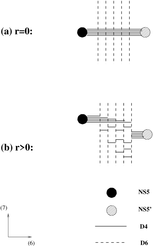
  FIG. 26.: Displacing the fivebranes in $x^{7}$ corresponds to a FI D-term in the worldvolume gauge theory.

• FI D-Term: In the gauge theory it is possible to turn on a D-term for $U(1)\subset U(N_{c})$

  $${\cal L}_{FI}=r\int d^{4}\theta\,{\rm Tr}\,V$$ (204)

  Note that – unlike the $N=2$ SUSY case (112) – here the D-term is a single real number $r$. For $0<N_{f}<N_{c}$ adding (204) breaks SUSY. For $N_{f}\geq N_{c}$ there are supersymmetric vacua in which the gauge symmetry is completely broken and the system is forced into a Higgs phase. In the brane description, the role of the FI D-term is played by the relative displacement of the $NS5$ and $NS5^{\prime}$-branes in the $x^{7}$ direction (Fig. 26). Clearly, when the two are at different values of $x^{7}$, a fourbrane stretched between them breaks SUSY. To preserve SUSY, all such fourbranes must break on $D6$-branes, which as we saw above is only possible for $N_{f}\geq N_{c}$ because of the s-rule. Once all fourbranes have been split, there is no obstruction to moving the $NS5$ and $NS5^{\prime}$-branes to different locations in $x^{7}$. At generic points in the Higgs phase, nothing special happens when the D-term is turned off. In the brane construction the reason is that once all $N_{c}$ $D4$-branes have been broken on $D6$-branes in a generic way, nothing special happens when the relative displacement of the two fivebranes in $x^{7}$ vanishes.

• Global Symmetries: Classical supersymmetric QCD with gauge group $SU(N_{c})$ and $N_{f}$ quarks has the global symmetry (165); quantum effects break it to (166). The anomaly is a quantum effect which is not expected to be visible in the classical brane construction (we will exhibit it in the brane description in section V C) .

  

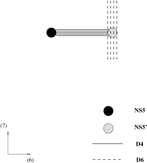
  FIG. 27.: Placing the $D6$ branes on the $NS5^{\prime}$-brane enhances the global symmetry at finite energies from $SU(N_{f})$ to $SU(N_{f})\times SU(N_{f})$.

  In our case, the (classical) gauge symmetry is $U(N_{c})\simeq SU(N_{c})\times U(1)$, with the extra $U(1)$ factor in the gauge group corresponding to gauging baryon number $U(1)_{B}$. The brane configuration has a manifest (vector) $SU(N_{f})$ symmetry, which is a gauge symmetry on the $D6$-branes and a global symmetry on the $D4$-branes. The other (axial) $SU(N_{f})$ symmetry is generically not an exact symmetry of the brane configuration of Fig. 24(b), and arises as an effective symmetry when we take the infrared limit. In the general spirit of brane theory – trying to realize as much as possible of the symmetry structure of the low energy theory throughout the RG flow – one might wonder whether it is possible to realize it too as an exact symmetry of the brane vacuum.

  This is indeed the case as shown by [55, 7, 124]. The main idea is the following. We saw before that the positions of the $D6$-branes in $x^{6}$ are not visible in the low energy theory, but of course their values influence the high energy structure. One may thus hope that the full chiral symmetry may be restored for some particular value of these parameters. When the $D6$-branes are placed at the same value of $x^{6}$ as the $NS5^{\prime}$-brane (Fig. 27) the full chiral symmetry is restored [55].

  To see that this is geometrically plausible, note that when that happens, the $NS5^{\prime}$-brane located at (say) $x^{7}=0$ cuts each $D6$-brane into two disconnected halves, the $x^{7}>0$ and $x^{7}<0$ parts . The situation is very similar to that encountered in section IV C 4 when we discussed compact Coulomb branches. Using our analysis there, it is clear that there are now two separate $SU(N_{f})$ symmetries acting on the two disconnected groups of $N_{f}$ sixbranes. Just like in section IV C 4, despite the fact that the two groups of sixbranes are independent, we cannot remove one of them from the configuration. From the brane theory point of view this is due to the fact that, as discussed in section IV C 4, this would lead to non-conservation of charge. From the point of view of the gauge theory on the fourbranes the reason is that the resulting four dimensional gauge theory, with only fundamentals and no antifundamentals, would be anomalous.

  The symmetries $U(1)_{x}$, $U(1)_{a}$ (165) are also realized in the brane picture. They correspond to rotations in the $(x^{4},x^{5})$ and $(x^{8},x^{9})$ planes, $U(1)_{45}$, $U(1)_{89}$. These rotations are $R$-symmetries because the four preserved supercharges of the brane configuration of Fig. 24 are spinors of the $Spin(9,1)$ Lorentz group in ten dimensions and, therefore, are charged under both $U(1)_{45}$ and $U(1)_{89}$. From the discussion of the mass deformations and Higgs moduli space above, it is clear that the mass parameters (202) are charged under $U(1)_{45}$, while the quarks $Q$, $\tilde{Q}$ are charged under $U(1)_{89}$. If we assign $U(1)_{45}\times U(1)_{89}$ charges $(1,1)$ to the superspace coordinates $\theta_{\alpha}$, the quarks $Q$ and $\tilde{Q}$ have charges $(0,1)$, while the mass parameters $m$ in (202) have charges $(2,0)$. With these assignments, the mass term (202) is invariant under both global symmetries .

2 Classical SQCD: The Magnetic Theory

The “magnetic” brane configuration – the reason for the name will become clear soon – contains $N_{c}$ $D4$-branes connecting the $NS5^{\prime}$-brane to an $NS5$-brane on its right (we will refer to these as “color fourbranes”), and $N_{f}$ $D4$-branes connecting the $NS5^{\prime}$-brane to $N_{f}$ $D6$-branes on its left, which we will refer to as “flavor fourbranes.” The configuration is depicted in Fig. 28. As usual, all the branes involved are stretched in the directions given in (105, 195). We will consider the case $N_{f}\geq N_{c}$ in what follows.

FIG. 28.: The magnetic brane configuration.

This configuration describes SQCD with “magnetic gauge group” $G_{m}=U(N_{c})$ (with the gauge bosons coming as before from $4-4$ strings connecting different color fourbranes), $N_{f}$ flavors of “magnetic quarks” $q_{i}$, $\tilde{q}^{i}$ ($4-4$ strings connecting the $N_{c}$ color fourbranes with the $N_{f}$ flavor fourbranes). In addition to the $N=1$ SQCD matter content there are now $N_{f}^{2}$ chiral superfields that are singlets under the gauge group $G_{m}$, arising from $4-4$ strings connecting different flavor fourbranes. Denoting these “magnetic meson” fields by $M^{i}_{j}$ $(i,j=1,\cdots,N_{f})$, it is clear that the standard coupling of three open strings gives rise to a superpotential connecting the magnetic mesons and the magnetic quarks,

$$W_{\rm mag}=M^{i}_{j}q_{i}\tilde{q}^{j}$$ (205)

This is precisely the “magnetic theory” discussed in section V A.

The analysis of moduli space and deformations of this model is similar to the electric theory, with a few differences due to the existence of the superpotential (205). Consider first mass deformations. In gauge theory we can add a mass term to the magnetic quarks, by modifying the superpotential to

$$W_{\rm mag}=M^{i}_{j}q_{i}\tilde{q}^{j}+\delta M^{i}_{j}q_{i}\tilde{q}^{j}$$ (206)

The mass parameters $\delta M$ can be absorbed in the expectation value of the magnetic meson $M^{i}_{j}$, and can be thought of as parametrizing a moduli space of vacua. The $N_{f}^{2}$ resulting parameters are described in the brane language by splitting the $N_{f}$ flavor fourbranes on the $D6$-branes in the most general way consistent with the geometry (Fig. 29(a)). This results in a total of $N_{f}^{2}$ massless modes corresponding to the $N_{f}^{2}$ components of $M$: $N_{f}$ of them describe fluctuations in the $(x^{8},x^{9})$ plane of fourbranes stretched between the $NS5^{\prime}$-brane and the rightmost $D6$-brane, and the remaining $\sum_{l=1}^{N_{f}-1}2l=N_{f}(N_{f}-1)$ parametrize fluctuations in $(x^{6},x^{7},x^{8},x^{9})$ of the fourbranes connecting different sixbranes.

FIG. 29.: (a) The $N_{f}^{2}$ dimensional classical magnetic moduli space corresponding to unbroken gauge symmetry and arbitrary expectation values for the singlet meson $M$. (b) The brane description of adding a linear superpotential $W=-mM$. The eigenvalues of $m$ correspond to locations of $D6$-branes in the $v$ plane.

Another interesting deformation of the magnetic gauge theory corresponds to adding a linear term in $M$ to the magnetic superpotential

$$W_{\rm mag}=M^{i}_{j}(q_{i}\tilde{q}^{j}-m_{i}^{j})$$ (207)

Integrating out the massive field $M$ we find that in the presence of the “mass parameters” $m_{i}^{j}$ the gauge group is broken; thus the parameters $m$ play the role of Higgs expectation values. In the brane description, these deformations correspond to a process where color fourbranes are aligned with flavor fourbranes and reconnected to stretch between the $NS5$-brane and a $D6$-brane (see Fig. 29(b)). If $m$ has rank $n(\leq N_{c})$, $n$ such fourbranes are reconnected. The $D6$-branes on which the reconnected fourbranes end can then be moved in the $(x^{4},x^{5})$ directions, taking the fourbranes with them and breaking the $U(N_{c})$ gauge group to $U(N_{c}-n)$. The brane description realizes only a subset of the possible “mass matrices” $m$, namely, those which satisfy (203) (the reason is similar to the one described there). We will soon see that this analogy is not coincidental.

Another deformation of the magnetic gauge theory and of the corresponding brane configuration, which will play a role in the sequel, is switching on a FI D-term for the $U(1)$ subgroup of $U(N_{c})$. Again, in the brane construction this corresponds to a relative displacement of the $NS5$ and $NS5^{\prime}$-branes in the $x^{7}$ direction (Fig. 30). To preserve SUSY, all $N_{c}$ color fourbranes have to be reconnected to $N_{c}$ of the $N_{f}$ flavor fourbranes, leading to a situation where $N_{c}$ fourbranes stretch between the $NS5$-brane and $N_{c}$ different sixbranes and $N_{f}-N_{c}$ fourbranes stretch between the $NS5^{\prime}$-brane and the remaining sixbranes (Fig. 29(b)). Once this occurs, the two fivebranes can be separated in $x^{7}$.

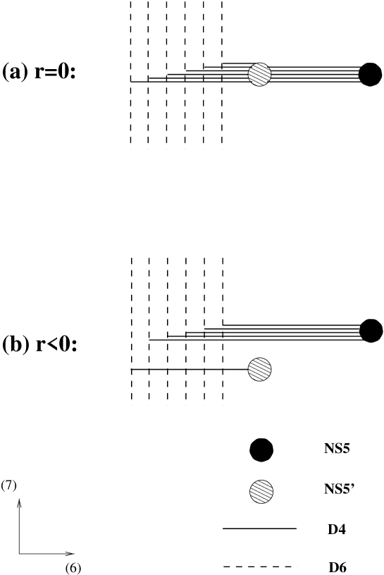
FIG. 30.: The brane description of the FI D-term in the magnetic theory.

Unlike the electric theory, here there is a jump in the dimension of the classical moduli space of the theory as we vary the D-term. For non-vanishing D-term there are only $N_{f}-N_{c}$ fourbranes that give rise to moduli (the other $N_{c}$ are frozen because of the s-rule), and the moduli space is easily checked to be $N_{f}^{2}-N_{c}^{2}$ dimensional. When the D-term vanishes, the previously frozen fourbranes can be reconnected to yield the original configuration, with unbroken $U(N_{c})$, and we gain access to the full $N_{f}^{2}$ dimensional moduli space of Fig. 29(a). We will see in section V C that quantum mechanically this classical jump in the structure of the moduli space disappears.

The magnetic brane configuration is invariant under the same global symmetries as the electric theory described above (165). The charge assignments under the $U(1)_{45}\times U(1)_{89}$ symmetry are as follows: the magnetic quarks $q$, $\tilde{q}$ have charges $(1,0)$, the mass parameters $m$ have charges $(2,0)$, the magnetic meson $M$ has charges $(0,2)$, and the superspace coordinates $\theta_{\alpha}$ have charges $(1,1)$.

3 Seiberg’s Duality In The Classical Brane Picture

We have now constructed using branes two $N=1$ supersymmetric gauge theories, the electric and magnetic theories discussed in the previous two subsections. Seiberg has shown that the electric gauge theory with gauge group $U(N_{c})$ and the magnetic theory with gauge group $U(N_{f}-N_{c})$ are equivalent in the extreme infrared  (i.e. they flow to the same infrared fixed point) [201]. Seiberg’s duality is a quantum symmetry, but it has classical consequences in situations where the gauge symmetry is completely broken and there is no strong infrared dynamics. In such situations Seiberg’s duality reduces to a classical equivalence of moduli spaces and their deformations.

In this subsection we show using brane theory that the moduli spaces of vacua of the electric and magnetic theories with gauge groups $U(N_{c})$ and $U(N_{f}-N_{c})$ coincide. They provide different parametrizations of the moduli space of vacua of the appropriate brane configuration. This explains the classical part of Seiberg’s duality. As one approaches the root of the Higgs branch, non-trivial quantum dynamics appears, and we have to face the resulting strong coupling problem. This will be addressed in section V C.

Start, for example, with the electric theory with gauge group $U(N_{c})$ (the configuration of Fig. 24(a)). Now enter the Higgs phase by connecting the $N_{c}$ original fourbranes stretched between the $NS5$ and $NS5^{\prime}$-branes to $N_{c}$ of the $N_{f}$ fourbranes stretched between the $NS5$-brane and the sixbranes; we then further reconnect the resulting fourbranes in the most general way consistent with the rules described in sections IV C 1, V B 1. The resulting moduli space is $2N_{f}N_{c}-N_{c}^{2}$ dimensional, as described in subsection V B 1. Note that, generically, there are now $N_{f}-N_{c}$ $D4$-branes attached to the $NS5$-branes, and $N_{c}$ $D4$-branes connected to the $NS5^{\prime}$-brane (the other ends of all these fourbranes lie on different $D6$-branes).

Once we are in the Higgs phase, we can freely move the $NS5$-brane relative to the $NS5^{\prime}$-brane and, in particular, the two branes can pass each other in the $x^{6}$ direction without ever meeting in space. This can be achieved by taking the $NS5$-brane around the $NS5^{\prime}$-brane in the $x^{7}$ direction, i.e. turning on a FI D-term in the worldvolume gauge theory (the process is described in Fig. 31). At a generic point in the Higgs branch of the electric theory, turning on such a D-term is a completely smooth procedure; this is particularly clear from the brane description, where in the absence of $D4$-branes connecting the $NS5$-brane to the $NS5^{\prime}$-brane, the relative displacement of the two in the $x^{7}$ direction can be varied freely.

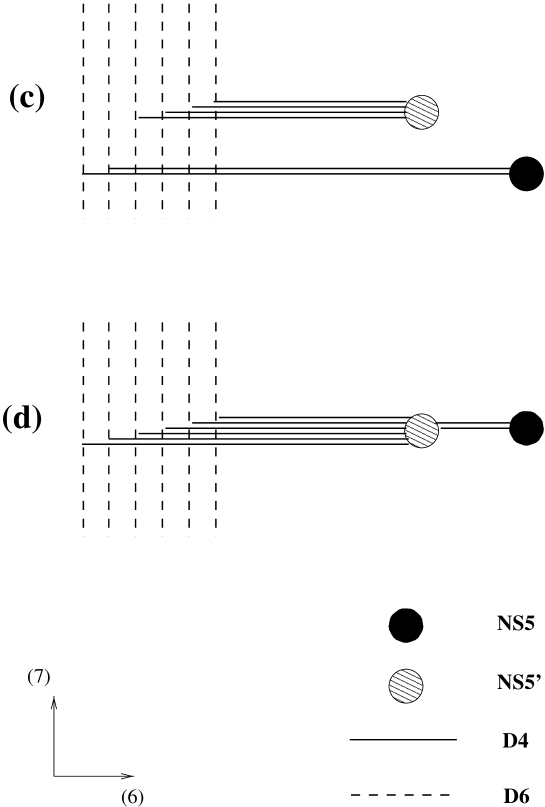
FIG. 31.: The electric and magnetic brane configurations are continuously connected in the way indicated here. Starting with the electric configuration (a), one can turn on a FI D-term (b), exchange the fivebranes in $x^{6}$ (c), and switch off the D-term, arriving at the magnetic configuration (d).

After exchanging the $NS5$ and $NS5^{\prime}$-branes, the brane configuration we find can be interpreted as describing the Higgs phase of another gauge theory. To find out what that theory is, we approach the root of the Higgs branch by aligning the $N_{f}-N_{c}$ $D4$-branes emanating from the $NS5$-brane with the $NS5^{\prime}$-brane, and the $N_{c}$ $D4$-branes emanating from the $NS5^{\prime}$-brane with $D4$-branes stretched between $D6$-branes.

We then reconnect the $D4$-branes to obtain a configuration consisting of $N_{f}-N_{c}$ $D4$-branes connecting the $NS5^{\prime}$-brane to an $NS5$-brane which is to the right of it; the $NS5^{\prime}$-brane is further connected by $N_{f}$ $D4$-branes to the $N_{f}$ $D6$-branes which are to the left of it (see Fig. 31(d)). This is the magnetic SQCD of subsection V B 2, with gauge group $U(N_{f}-N_{c})$.

To summarize, we have shown that the moduli space of vacua of the electric SQCD theory with (completely broken) gauge group $U(N_{c})$ and $N_{f}$ flavors of quarks, and the moduli space of vacua of the magnetic SQCD model with (broken) gauge group $U(N_{f}-N_{c})$, can be thought of as providing different descriptions of a single moduli space of supersymmetric brane configurations. One can smoothly interpolate between them by varying the scale $\Lambda$ (related to the displacement of the $NS5$ and $NS5^{\prime}$-branes in $x^{6}$), keeping the FI D-term fixed but non-zero. Since the only role of $\Lambda$ in the low energy theory is to normalize the operators [156], theories with different values of $\Lambda$ are equivalent. The electric and magnetic theories will thus share all features, such as the structure of the chiral ring (which can be thought of as the ring of functions on moduli space), that are independent of the interpolation parameter $\Lambda$.

The above smooth interpolation relies on the fact that the gauge symmetry is completely broken due to the presence of the FI D-term. As mentioned above, it is not surprising that duality appears classically in this situation since there is no strong infrared gauge dynamics.

The next step is to analyze what happens as the gauge symmetry is restored when the D-term goes to zero and we approach the origin of moduli space. Classically, we find a disagreement. In the electric theory, we saw in subsection V B 1 that nothing special happens when the gauge symmetry is restored. New massless degrees of freedom appear, but there are no new branches of the moduli space that we gain access to.

In the magnetic theory the situation is different. When we set the FI D-term to zero, we saw in subsection V B 2 that a large moduli space of previously inaccessible vacua becomes available. While the electric theory has a $2N_{f}N_{c}-N_{c}^{2}$ dimensional smooth moduli space, the classical magnetic theory experiences a jump in the dimension of its moduli space from $2N_{f}N_{c}-N_{c}^{2}$ for non-vanishing FI D-term to $N_{f}^{2}$ when the D-term is zero. However, in the magnetic theory when the D-term vanishes the $U(N_{f}-N_{c})$ gauge symmetry is restored, and to understand what really happens we must study the quantum dynamics. We will discuss this in section V C, where we shall see that quantum mechanically the jump in the magnetic moduli space disappears, and the quantum moduli spaces of the electric and magnetic theories agree.

It is instructive to map the deformations of the classical electric theory to those of the classical magnetic one. Turning on masses (202) in the electric theory corresponds to moving the $D6$-branes away from the $D4$-branes (or equivalently from the $NS5^{\prime}$-brane) in the $(x^{4},x^{5})$ directions. As discussed in subsection V B 2, in the magnetic description, the electric mass parameters correspond to Higgs expectation values (207).

Turning on expectation values to the electric quarks, which was described in the brane language in subsection V B 1, corresponds on the magnetic side to varying the expectation value of the magnetic meson $M$ (206). This gives masses to the magnetic quarks.

The transmutation of masses into Higgs expectation values and vice-versa observed in the brane construction is one of the hallmarks of Seiberg’s duality.

4 Other Rotated $N=2$ Configurations

The brane configurations corresponding to electric and magnetic SQCD were obtained above by rotating branes in the $N=2$ SUSY configuration studied in section IV. Before moving on to the study of quantum dynamics of these theories we would like to discuss a few additional theories that can be realized using such rotations.

1. ${\bf U(N_{c})}$ With Adjoint, ${\bf N_{f}}$ Flavors And ${\bf W=0}$

Starting with the $N=2$ SUSY brane configuration of Fig. 14, rotate the two $NS5$-branes as in (192-194) keeping them parallel to each other. As discussed above (197) the angle of rotation determines the Yukawa coupling; in particular, when the two $NS5$-branes are rotated into $NS5^{\prime}$-branes (Fig. 32(a)) the Yukawa coupling disappears. The resulting theory has gauge group $U(N_{c})$, the matter content necessary for $N=2$ SUSY, i.e. an adjoint chiral multiplet $\Phi$ and $N_{f}$ fundamentals $Q^{i}$, $\tilde{Q}_{i}$, but the superpotential $W=\tilde{Q}\Phi Q$ required by $N=2$ SUSY in $4d$ is absent here; instead, $W=0$. This is a model discussed in subsection V A 3.

FIG. 32.: (a) $N=1$ SYM with $G=U(N_{c})$, $N_{f}$ fundamentals, and an adjoint superfield with vanishing superpotential. (b) The fully Higgsed branch of moduli space.

Fluctuations of the $N_{c}$ fourbranes along the $NS5^{\prime}$-branes parametrize the Coulomb branch of the model. Displacements of the $N_{f}$ $D6$-branes relative to the $NS5^{\prime}$-branes in the $(x^{4},x^{5})$ directions give masses $m$ to the fundamental multiplets $Q$, $\tilde{Q}$

$$W=-\sum_{i=1}^{N_{f}}m_{i}\tilde{Q}_{i}Q^{i}$$ (208)

The relative position of the two $NS5^{\prime}$-branes in the $(x^{4},x^{5})$ directions is not an independent parameter; it can be compensated by a change in the positions of the $D6$-branes in the $(x^{4},x^{5})$ plane (i.e. the masses of the fundamentals), and an overall rotation of the configuration. The relative displacement of the two $NS5^{\prime}$-branes in the $x^{7}$ direction plays the role of a FI D-term (204). Complete Higgsing is possible for all $N_{f}\geq 1$; the (complex) dimension of the Higgs branch is

$${\rm dim}{\cal M}_{H}=2N_{f}N_{c}+N_{c}^{2}-N_{c}^{2}=2N_{f}N_{c}$$ (209)

The first two terms on the left hand side are the numbers of components in the fundamental and adjoint chiral multiplets, and the negative term accounts for degrees of freedom eaten up by the Higgs mechanism.

The brane configuration provides a simple picture of the moduli space of vacua. As usual, complete Higgsing corresponds to breaking all $N_{c}$ fourbranes on various $D6$-branes as indicated in Fig. 32(b). We find that the dimension of moduli space of brane configurations with completely broken $U(N_{c})$ gauge symmetry is

$${\rm dim}{\cal M}_{H}=N_{c}\left[2(N_{f}-1)+1+1\right]=2N_{c}N_{f}$$ (210)

in agreement with the gauge theory analysis (209).

2. Mixed Electric-Magnetic Theories

A straightforward generalization of the electric and magnetic SQCD brane configurations is a configuration which includes both “electric” and “magnetic” quarks. Consider the configuration of Fig. 33; an $NS5$-brane connected by $N_{c}$ $D4$-branes to an $NS5^{\prime}$-brane which is to its right (in $x^{6}$). To the left of the $NS5$-brane we put $N_{f}$ $D6$-branes each of which is connected by a fourbrane to the $NS5$-brane. As before, these represent $N_{f}$ quarks $Q,\tilde{Q}$. To the right of the $NS5^{\prime}$-brane we put $N^{\prime}_{f}$ $D6$-branes each of which is connected to the $NS5^{\prime}$-brane by a fourbrane. These represent $N^{\prime}_{f}$ quarks $Q^{\prime},\tilde{Q}^{\prime}$ and $N^{\prime 2}_{f}$ complex scalars $M^{\prime}$ with a tree level superpotential $W=M^{\prime}Q^{\prime}\tilde{Q}^{\prime}$. The SYM theory thus obtained is a “mixed electric-magnetic” $SU(N_{c})$ gauge theory with $N_{f}$ “electric” quarks and $N^{\prime}_{f}$ “magnetic” quarks coupled to “magnetic mesons.”

The discussion of Seiberg’s duality can be repeated for such theories. Interchanging the two NS-branes in $x^{6}$ gives rise to an $SU(N_{f}+N^{\prime}_{f}-N_{c})$ theory with $N_{f}$ magnetic quarks $q,\tilde{q}$ coupled to $N_{f}^{2}$ complex scalars $M$ via $Mq\tilde{q}$, and $N^{\prime}_{f}$ electric quarks $q^{\prime},\tilde{q}^{\prime}$. Of course, the dual theory is also a mixed electric-magnetic theory where the role of electric and magnetic quarks is interchanged. In the particular case $N^{\prime}_{f}=0$ the original theory is the electric theory studied in section V B 1 while its dual is the magnetic theory as considered in section V B 3.

FIG. 33.: A “mixed electric-magnetic” theory, in which some of the fundamentals couple to singlet mesons and some do not.

3. ${\bf D6^{\prime}}$-Branes

Another interesting deformation of the $N=2$ SUSY configuration involves rotating some of the $D6$-branes as well. Restricting our attention to ninety degree rotations, for simplicity, we would like to consider, in addition to the objects studied above, rotated sixbranes that are located at $w=0$ and stretched in $v$. We will refer to them as $D6^{\prime}$-branes:

$$D6^{\prime}:\qquad(x^{0},x^{1},x^{2},x^{3},x^{4},x^{5},x^{7})$$ (211)

To study brane configurations including both $D6$ and $D6^{\prime}$-branes one has to keep in mind the following interesting feature of brane dynamics.

Consider a configuration in which a pair of $D4$-branes connect a $D6$-brane to a $D6^{\prime}$-brane. Naively the configuration preserves four supercharges and there are two complex moduli describing the locations of the two $D4$-branes along the sixbranes (in $x^{7}$) together with the compact component of the gauge field $A_{6}$.

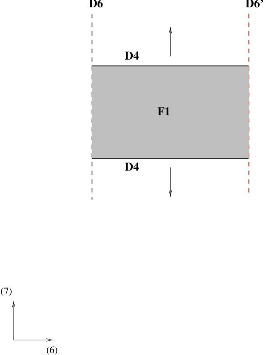
FIG. 34.: The repulsive interaction between $D4$-branes stretched between $D6$ and $D6^{\prime}$-branes is due to Euclidean fundamental strings stretched between the various branes.

However, there is a superpotential due to Euclidean fundamental strings stretched between the $D4$ and $D6$-branes, as indicated in Fig. 34. If the distance between the sixbranes is $\delta l_{6}$ and the separation between the fourbranes is $\delta l_{7}$, the superpotential due to these Euclidean strings is of order $\exp(-\delta l_{6}\delta l_{7}/l_{s}^{2})$. This effect is non-perturbative in $l_{s}$ but does not go to zero in the limit $g_{s}\to 0$ – it is a worldsheet instanton effect. In particular, it does not vanish in the classical gauge theory limit discussed above and leads to long range repulsive interactions between the fourbranes. It is closely related to the non-perturbative effects discussed in section III in systems with twice as much SUSY, where they contribute to the metric on moduli space (see eq. (82)).

We thus arrive at the following classical rule of brane dynamics:

There is a long range repulsive interaction between $D4$-branes stretched between a $D6$-brane and a $D6^{\prime}$-brane. This repulsion does not go to zero in the classical limit $g_{s}\to 0$.

Taking this rule into account allows one to understand configurations including both $D6$ and $D6^{\prime}$-branes. The resulting physics depends on the ordering of the sixbranes along the $x^{6}$ axis. When a $D6$-brane passes a $D6^{\prime}$-brane there is a phase transition; this can be seen by U-duality which can be used to map this system to an $NS5^{\prime}$-brane and a $D6$-brane; as we saw before, the physics certainly changes when we exchange those. We will next consider the physics for a particular ordering of the branes; the generalization to other cases is straightforward.

Consider the configuration of Fig. 35. In addition to the usual $N_{c}$ $D4$-branes stretched between $NS5$ and $NS5^{\prime}$-branes, which give rise to a $U(N_{c})$ gauge group, we have $N_{f}$ $D6$-branes located next to the $NS5^{\prime}$-brane and $N_{f}^{\prime}$ $D6^{\prime}$-branes located next to the $NS5$-brane, which give rise to $N_{f}+N_{f}^{\prime}$ flavors. Clearly the theory does not have a massless adjoint field as there is no Coulomb branch, and by placing the $D6$-branes on top of the $NS5^{\prime}$-brane and the $D6^{\prime}$-branes on top of the $NS5$-brane we deduce that the symmetry of the theory is at least $SU(N_{f})\times SU(N_{f})\times SU(N_{f}^{\prime})\times SU(N_{f}^{\prime})$, which does not allow a superpotential.

The theory is, therefore, $N=1$ SQCD with gauge group $U(N_{c})$, $N_{f}+N_{f}^{\prime}$ flavors of quarks and $W=0$, which we have analyzed before. The analysis of the moduli space gives the right structure; we leave the details to the reader. To get the correct structure it is important to use the rule stated above, which implies here that configurations in which multiple $D4$-branes connect a given $D6$ and $D6^{\prime}$-brane are unstable.

FIG. 35.: $N=1$ SQCD with vanishing superpotential described by a configuration with both $D6$ and $D6^{\prime}$-branes.

C Quantum Effects

In this section we study quantum effects in $N=1$ SYM using brane theory. We describe the quantum moduli space of vacua and complete the demonstration of Seiberg’s duality. We start by following a similar route to that taken in section IV, and study the form of the M-theory fivebrane describing the brane configuration at finite $R_{10}/L_{6}$, first semiclassically and then exactly. Then we present a qualitative picture of the moduli space as resulting from certain quantum interactions between branes analogous to the classical interactions encountered in the last subsection.

1 Semiclassical Description

At finite gauge coupling $g$ (107) we should interpret our brane configurations as describing fivebranes and sixbranes in M-theory with finite $R_{10}/L_{6}=l_{s}g_{s}/L_{6}$. Recall the definitions

$$s= x^{6}+ix^{10}$$ (212)

$$v= x^{4}+ix^{5}$$ (213)

$$w= x^{8}+ix^{9}$$ (214)

Classically, i.e. ignoring the size of the $x^{10}$ circle, the $D4$-brane is located at $v=w=0$ and is extended in $s$, the $NS5$-brane is at $s=w=0$ and is extended in $v$, while the $NS5^{\prime}$-brane is at $v=0$, $s=L_{6}$ and is extended in $w$.

Quantum mechanically, the fourbranes and fivebranes merge into a single fivebrane in M-theory, as described in the $N=2$ case in section IV. The vacuum configuration of the fivebrane is described by a curve $\Sigma$ embedded in the space $R^{5}\times S^{1}$ (214). As before, for large $v$, $w$ we can think of the shape of the resulting $M5$-brane in terms of the original $NS5$ and $NS5^{\prime}$-branes, appropriately deformed by the fourbranes ending on them (118). The structure for large $v$, $w$ is the brane analog of one loop corrections to classical physics in gauge theory. In this subsection we will describe these effects [89].

Consider the classical electric configuration of Fig. 24(a). According to (118), far from the origin this configuration is deformed as follows. For large $v$ (and small $w$), the shape of the $M5$-brane is that of the deformed $NS5$-brane

$$s_{5}=(N_{f}-N_{c})R_{10}\log v$$ (215)

while for large $w$ (and small $v$) it looks like the deformed $NS5^{\prime}$-brane

$$s_{5^{\prime}}=N_{c}R_{10}\log w$$ (216)

The two asymptotic regions join in a way that will be discussed later at small $v$, $w$.

As explained in section IV C 4, among other things, this bending causes the freezing of the $U(1)\subset U(N_{c})$. Therefore, quantum mechanically we are dealing with an $SU(N_{c})$ gauge theory.

In subsection V A we saw that the classical electric SQCD is invariant under two $U(1)$ $R$-symmetries (165). In gauge theory only one combination of the two is preserved quantum mechanically; the other is broken by the chiral anomaly or, equivalently, instantons (see section V A). We will next exhibit this effect in brane theory.

The two classical $R$-symmetries correspond in the brane construction to rotations of the $(x^{4},x^{5})$ plane, $v\to e^{i\alpha}v$, and the $(x^{8},x^{9})$ plane, $w\to e^{i\beta}w$. The semiclassical configuration (215, 216) breaks both symmetries. ${\rm Re}s_{5}$ and ${\rm Re}s_{5^{\prime}}$ are invariant under $U(1)_{45}$ and $U(1)_{89}$, but ${\rm Im}s_{5}$ and ${\rm Im}s_{5^{\prime}}$ are not invariant. Overall shifts of ${\rm Im}s$ can be compensated by a translation in $x^{10}$, hence any combination of $U(1)_{45}$ and $U(1)_{89}$ which preserves the relative location of the $NS5$ and $NS5^{\prime}$-branes in $x^{10}$ is a symmetry. The (semiclassically) unbroken $R$-symmetry is, therefore, the one which preserves

$$s_{5}-s_{5^{\prime}}=R_{10}\log\left(w^{-N_{c}}v^{N_{f}-N_{c}}\right)$$ (217)

It is not difficult to check that if (by definition) the $R$-charge of $\theta$ under this symmetry is one, that of $Q$, $\tilde{Q}$ is $R(Q)=R(\tilde{Q})=1-N_{c}/N_{f}$, in agreement with the gauge theory answer (167). Of course, so far all we have checked is that this symmetry is conserved semiclassically. In field theory there is no contribution to the anomaly beyond one loop; brane dynamics reflects that, and one can check that the exact form of the fivebrane preserves the symmetry as well.

One can tell the same story for the brane construction describing magnetic SQCD. The classical $R$-symmetry corresponds again to $U(1)_{45}\times U(1)_{89}$. The charge assignments of the various fields ($q$, $\tilde{q}$, $M$) agree with those found in gauge theory (see section V A) and with the electric configuration. Quantum mechanically the fivebranes are deformed due to the presence of the fourbranes; equations (215), (216) which were found for the electric configuration, are valid for the magnetic one as well. In brane theory this is a consequence of the fact that the two configurations are related by the smooth transition discussed earlier. In gauge theory it is one of the checks of Seiberg’s duality.

The foregoing discussion may be used to provide a heuristic explanation of a certain scale matching relation between the electric and magnetic theories used in gauge theory studies of Seiberg’s duality. We can think of the electric coupling $(s_{5}-s_{5^{\prime}})/R_{10}$ (217) as describing the electric QCD scale $\Lambda_{e}$:

$$\Lambda_{e}^{3N_{c}-N_{f}}=\mu^{3N_{c}-N_{f}}e^{-(s_{5}-s_{5^{\prime}})/R_{10}}=\mu^{3N_{c}-N_{f}}w^{N_{c}}v^{N_{c}-N_{f}}$$ (218)

where $\mu$ is some fixed scale. If we start with a large and negative ${\rm Re}(s_{5}-s_{5}^{\prime})$ the QCD scale $\Lambda_{e}$ is large. Exchanging the branes as discussed above leads to a theory with ${\rm Re}(s_{5}-s_{5}^{\prime})>0$ and, therefore, small $\Lambda_{e}$. In this situation we can continue thinking about the theory as the electric theory with a small $\Lambda_{e}$; alternatively, we can switch to the magnetic point of view and define the magnetic QCD scale $\Lambda_{m}$:

$$\Lambda_{m}^{3\bar{N}_{c}-N_{f}}=\mu^{3\bar{N}_{c}-N_{f}}e^{+(s_{5}-s_{5^{\prime}})/R_{10}}$$ (219)

where $\bar{N}_{c}\equiv N_{f}-N_{c}$. Equations (218), (219) lead to the scale matching relation

$$\Lambda_{e}^{3N_{c}-N_{f}}\Lambda_{m}^{3\bar{N}_{c}-N_{f}}=\mu^{N_{f}}$$ (220)

which has been argued to hold in gauge theory, with $\mu$ a constant related to the coefficient of the magnetic superpotential (181) [156]. The relation (220) emphasizes the strong-weak coupling aspect of Seiberg’s duality, since if $\Lambda_{e}$ becomes small (thus making the electric theory weakly coupled) $\Lambda_{m}$ is large, and vice-versa.

2 Exact Results

So far we have focused on the large $v$, $w$ form of the $M5$-brane into which the IIA fivebranes and fourbranes merge for finite $R_{10}/L_{6}$. Following the logic of section IV we next derive its exact form.

We start with the case of pure SYM with $G=SU(N_{c})$ and no matter, described by the brane configuration of Fig. 24 (without sixbranes). We can proceed as in the $N=2$ case studied in section IV. The worldvolume of the $M5$-brane is $R^{3,1}\times\Sigma$, where the complex curve $\Sigma$ is now embedded in the three complex dimensional space $Q\simeq R^{5}\times S^{1}$ parametrized by $(v,w,s)$. The shape of the curve $\Sigma$ can be determined by using the symmetries and singularity structure [132, 238].

Defining the variable $t$ as in (119), we know that as $v\to\infty$ on $\Sigma$ (the region corresponding to the $NS5$-brane), $t$ diverges (215) as $t\simeq v^{N_{c}}$, while $w$ goes to zero. Similarly, as $w\to\infty$ (the $NS5^{\prime}$-brane (216)), $t\simeq w^{-N_{c}}$ while $v\to 0$. More generally, $t$ should be a function of $v$ that does not have poles or zeroes except at $v=0$ (which is $w=\infty$) and $v=\infty$. The unique solution to all the constraints, up to an undetermined constant $\zeta$, is:

$$v^{N_{c}}=t$$ (221)

$$w^{N_{c}}=\zeta^{N_{c}}t^{-1}$$ (222)

$$vw=\zeta$$ (223)

One way of arriving at the curve (223), which also helps to understand the role of the parameter $\zeta$, is to start with the $N=2$ SUSY configuration described in section IV, and rotate one of the $NS5$-branes as described in subsection V B [132, 238].

The $N=2$, $SU(N_{c})$ brane configuration is given by the curve (121-123)

$$t^{2}+B(v,u_{k})t+\Lambda_{N=2}^{2N_{c}}=0$$ (224)

where we have restored the dependence on the QCD scale $\Lambda_{N=2}$. We would like to find the curve corresponding to a configuration where the right $NS5$-brane has been rotated as in (192-194), which corresponds to turning on a (complex) mass $\mu$ to the adjoint field (196), breaking $N=2$ SUSY to $N=1$. In order to “rotate the $NS5$-brane” we must consider configurations where the genus $N_{c}-1$ curve (224) degenerates to a genus zero one. In gauge theory this is the statement that the adjoint mass lifts the Coulomb branch, except for isolated points. In the classical IIA limit there is one such point, where all the $D4$-branes are placed together, corresponding to the origin of the Coulomb branch. For finite $R_{10}/L_{6}$ there are $N_{c}$ points where the curve (224) is completely degenerate. These points are related by the discrete unbroken $Z_{2N_{c}}$ subgroup of $U(1)_{45}$ whose action on $v$, $t$ was described in section IV C 4 (after eq. (132)). It acts on the QCD scale as:

$$\Lambda_{N=2}^{2}\to e^{2\pi i\over N_{c}}\Lambda_{N=2}^{2}$$ (225)

At one of these degenerate points the curve takes the form

$$v=t^{1/N_{c}}+\Lambda_{N=2}^{2}t^{-1/N_{c}}$$ (226)

Rotating the right $NS5$-brane from $w=0$ to $w=\mu v$ implies that at large $t$ we would like the curve to approach $v^{N_{c}}=t$ and $w$ to be small, while for $t\to 0$ we want it to approach $w=\mu v$ with large $v$, $w$ (corresponding to the $NS_{\theta}$ brane). This is achieved by supplementing (226) by:

$$w=\mu\Lambda_{N=2}^{2}t^{-1/N_{c}}$$ (227)

To make contact with (223) we would like to take the adjoint mass $\mu\to\infty$. Scale matching between the high energy theory with the adjoint field and the low energy theory obtained by integrating it out,

$$\Lambda_{N=1}^{3}={\mu\over N_{c}}\Lambda_{N=2}^{2}$$ (228)

implies that at the same time we have to take $\Lambda_{N=2}\to 0$ holding the $N=1$ SYM scale (228) fixed. Rewriting equations (226, 227) in terms of $\Lambda_{N=1}$,

$$v=t^{1/N_{c}}+{N_{c}\over\mu}\Lambda_{N=1}^{3}t^{1/N_{c}}$$ (229)

$$w=N_{c}\Lambda_{N=1}^{3}t^{-1/N_{c}}$$ (230)

and dropping the term proportional to $\mu^{-1}$ in the first equation of (230), leads to the curve (223) with 

$$\zeta=N_{c}\Lambda^{3}$$ (231)

We saw earlier that pure $N=1$ SYM with $G=SU(N_{c})$ has a $U(1)_{R}$ symmetry that is broken at one loop to $Z_{2N_{c}}$ by the chiral anomaly, and is further spontaneously broken non-perturbatively to $Z_{2}$, giving rise to $N_{c}$ vacua with different values of the gaugino condensate (158, 159). This pattern of breaking of the chiral $U(1)_{R}$ symmetry has a direct analog in the brane language. In the previous subsection we saw that the brane analog of the one loop effect of the anomaly is the asymptotic curving of the branes for large $v$, $w$. Thus studying the fivebrane (223) semiclassically is tantamount to having access to its large $v$, $w$ asymptotics, described by the first two equations in (223), but not to the shape of the fivebrane for small $v$, $w$ which is described by the last equation in (223).

It is therefore interesting that $\zeta$ appears in the first two equations only in the combination $\zeta^{N_{c}}$, while the third equation depends on $\zeta$ itself. This means that fivebranes (223) related by the $Z_{N_{c}}$ transformation

$$\zeta\to e^{2\pi i\over N_{c}}\zeta$$ (232)

look the same asymptotically (or semiclassically) but differ in their detailed shape. Each of the $N_{c}$ possible values of $\zeta$ (232) corresponds to a different fivebrane and, therefore, to a different vacuum of the quantum theory. The $Z_{N_{c}}$ symmetry relating them is spontaneously broken. One can think of $\zeta$ as the gaugino condensate (159) [132, 50].

In addition to the $Z_{N_{c}}$ symmetry mentioned above, which acts on $v$, $w$ and $t$ as

$$v\to v$$ (233)

$$w\to e^{2\pi i\over N_{c}}w$$ (234)

$$t\to t$$ (235)

and which – as explained above – is a symmetry of the first two equations in (223) but does not leave invariant the third one (or in other words has to be combined with (232) to become a symmetry), there are two more global symmetries. One is a $U(1)$ $R$-symmetry discussed near eq. (217),

$$v\to e^{i\delta}v$$ (236)

$$w\to e^{-i\delta}w$$ (237)

$$t\to e^{iN_{c}\delta}t$$ (238)

As anticipated there, this symmetry that is preserved semiclassically, is an exact symmetry of the brane configuration. For $N_{f}>0$ it corresponds to a symmetry of the low energy SYM theory, becoming part of the $N=1$ superconformal algebra in the IR. In the case considered here, in the absence of matter ($N_{f}=0$), the SYM fields do not carry charge under this symmetry. It is possible that this $U(1)$ symmetry is still part of the $N=1$ superconformal algebra in the infrared, but pure SYM theory has a mass gap and does not contribute to the extreme infrared CFT. If the brane configuration is to describe SYM physics at low but non-zero energies, any states charged under (238) must decouple from SYM physics.

There is also a $Z_{2}$ symmetry corresponding to exchanging $v$ and $w$,

$$v\to w$$ (239)

$$w\to v$$ (240)

$$t\to\zeta^{N_{c}}t^{-1}$$ (241)

This symmetry reverses the orientation of $4-4$ strings stretched between different fourbranes and, therefore, acts as charge conjugation. The fact that it is an exact symmetry of the vacuum is in agreement with gauge theory.

Having understood chiral symmetry breaking in the brane language we next turn to confinement [238]. Pure $N=1$ SYM is expected to have the property that if one introduces a heavy quark and antiquark into the system, the energy of the pair will grow with their separation as if the two were connected by a string with tension $\Lambda^{2}$. This “QCD string” can thus end on external quarks, but in the absence of quarks it is stable. Since $N_{c}$ fundamentals of $SU(N_{c})$ can combine into a singlet, QCD strings can annihilate in groups of $N_{c}$. It is expected that large $N_{c}$ QCD can be reformulated in terms of weakly coupled QCD strings. Establishing the existence and studying the properties of QCD strings is one of the major challenges in QCD.

In brane theory it is natural to identify the QCD string with an $M2$-brane ending on the $M5$-brane (223). We are searching for a membrane which looks like a string to a four dimensional observer and is also a string in the space $Q$ labeled by $(v,w,t)$. We can describe the string in $Q$ by an open curve $C$ parametrized by $0\leq\sigma\leq 1$, such that both of its endpoints (the points with $\sigma=0,1$) are in $\Sigma$. It turns out that the right curve for describing a QCD string is:

$$t=t_{0}={\rm const}$$ (242)

$$v=t_{0}^{1/N_{c}}e^{2\pi i\sigma/N_{c}}$$ (243)

$$vw=\zeta$$ (244)

The string in spacetime obtained by wrapping a membrane around the curve $C$ has the following properties:

1. Groups of $N_{c}$ (but not less) strings can annihilate.

2. The QCD string can end on an external quark.

3. For a particular choice of $t_{0}$, $C$ has minimal length.

The fact that QCD strings annihilate in groups of $N_{c}$ can be seen by aligning strings described by curves $C_{j}$ of the form (244) with $2(j-1)\pi\leq 2\pi\sigma\leq 2j\pi$ ($j=1,\cdots,N_{c}$). The $N_{c}$ strings form a long closed string in $Q$ which can detach from the fivebrane and shrink to a point. At the same time, the strings corresponding to different $C_{j}$ are all equivalent as they can be mapped into each other by continuously varying the phase of $t_{0}$, $t_{0}\to t_{0}\exp(2\pi i\alpha)$ with $0\leq\alpha\leq 1$.

To minimize the length of $C$ one notes that $t$ is constant along it, while $v$ and $w$ change by amounts of order $t_{0}^{1/N_{c}}/N_{c}$ and $\zeta t_{0}^{-1/N_{c}}/N_{c}$, respectively (for large $N_{c}$). The length is minimized for $t_{0}\sim\zeta^{N_{c}/2}$; it is of order $l_{C}\sim\zeta^{1/2}/N_{c}$. The tension of the QCD string is obtained by multiplying $l_{C}$ by the tension of the $M2$-brane $1/l_{p}^{3}$. Restoring dimensions in (231), $\zeta=N_{c}l_{p}^{6}\Lambda^{3}/R_{10}$, we find that the tension of the QCD string is

$$T\sim\left({\Lambda^{3}\over R_{10}N_{c}}\right)^{1\over 2}$$ (245)

In SYM one expects the tension of the QCD string to be of order $T\sim\Lambda^{2}$. Comparing to (245) we see that for agreement with SYM we must choose

$$R_{10}\sim{1\over N_{c}\Lambda}$$ (246)

For such values of $R_{10}$ there is no decoupling of the four dimensional SYM physics from Kaluza-Klein excitations carrying momentum in the $x^{10}$ direction. One might think that, due to (246), at least for large $N_{c}$ the Kaluza-Klein scale would be much higher than the QCD scale $\Lambda$. Unfortunately, since the Riemann surface $\Sigma$ winds $N_{c}$ times around the $x^{10}$ direction, the Kaluza-Klein modes see an effective radius $N_{c}R_{10}$ and have energies of order $\Lambda$. Thus decoupling fails even in the large $N_{c}$ limit.

From the discussion in previous sections it is clear what went wrong. The QCD string is not a BPS saturated object and, therefore, its tension is not protected by the usual non-renormalization theorems. The estimate (245) of its tension is semiclassical in nature and is valid when the supergravity approximation for describing membranes and fivebranes is applicable. We are discovering that in this regime the system does not describe decoupled SYM physics. The regime corresponding to SYM is (107-109); in that regime it is not clear at present how to study properties of the QCD string, such as the tension, but there is no reason for the formula (245) to be valid. It is known [66] that other non-holomorphic SYM features, such as the Kähler potential for mesons and baryons, depend sensitively on $R_{10}$, $L_{6}$, and there is no reason to expect that the tension of QCD strings is any different.

In addition to QCD strings, one can construct using branes domain walls separating regions in space corresponding to different vacua (different values of $\zeta$). A domain wall occurs when as $x^{3}\to-\infty$ the configuration approaches one value of $\zeta$ while as $x^{3}\to\infty$ it approaches another. The resulting $M5$-brane interpolates between the two solutions (223). It is known in gauge theory that such domain walls are BPS saturated and their tension is the difference between the values of the superpotential (160) between the different vacua. At large $N_{c}$ it thus goes like $T_{D}\simeq N_{c}\Lambda^{3}$.

Unlike the QCD string, the tension of the BPS saturated domain wall (or membrane) can be exactly calculated using branes. Witten has shown that the tension of the domain wall goes at large $N_{c}$ like $T_{D}\simeq R_{10}|\zeta|/l_{p}^{6}$ which, using the form of $\zeta$ and $R_{10}$ discussed above, agrees with the gauge theory analysis. Witten furthermore pointed out that the domain wall behaves in large $N_{c}$ gauge theory like a Dirichlet two brane in string theory; its tension goes like $N_{c}$, which is the inverse QCD string coupling, and the QCD string can end on it, just like the fundamental string can end on a D-brane.

The above discussion can be generalized by adding $N_{f}$ fundamental chiral multiplets of $SU(N_{c})$ with masses $m_{i}$, $i=1,\cdots,N_{f}$. We saw that these can be described by adding $N_{f}$ semi-infinite fourbranes to the left of the $NS5$-brane at $v=m_{i}$. The corresponding Riemann surface $\Sigma$ takes the form [132, 238, 50]

$$v^{N_{c}}=t\prod_{i=1}^{N_{f}}\left(1-{v\over m_{i}}\right)$$ (247)

$$vw=\zeta$$ (248)

where

$$\zeta^{N_{c}}=\Lambda^{3N_{c}-N_{f}}\prod_{i=1}^{N_{f}}m_{i}$$ (249)

For large $m_{i}$ the configuration (248) is essentially the same as (223) and one can think of the quarks with masses $m_{i}$ as static sources.

Quarks are confined in this system, and one expects the energy of a state with a quark and antiquark separated by a large distance $\delta x\gg\Lambda^{-1}$ to grow like $T\delta x$ where $T$ is the tension of the QCD string. Classically, the quark and antiquark are described by fundamental strings connecting a flavor fourbrane to the stack of color fourbranes. Quantum mechanically these fundamental strings turn into membranes and the only stable configuration has them connected by a long QCD string; thus its energy is indeed proportional to the separation of the two quarks as expected from gauge theory.

To study theories with massless quarks we have to take the limit $m_{i}\to 0$ (249). This was discussed in [132]. For $0<N_{f}<N_{c}$ massless flavors, the curve one finds in the limit is singular – it is infinitely elongated in the $x^{6}$ direction and, therefore, the corresponding brane configuration does not describe a four dimensional field theory. This is consistent with the field theory analysis: the gauge theory has no vacuum due to the non-perturbative superpotential (172).

For $N_{f}\geq N_{c}$ the SYM theories under consideration have quantum moduli spaces of vacua that were described in section V A. To study them one needs to replace the semi-infinite fourbranes by fourbranes ending on sixbranes, described as in section IV by an $M5$-brane in the background of a resolved $A_{N_{f}-1}$ multi Taub-NUT space. It is then possible, by rotating the $N=2$ SYM curves with matter studied in section IV, to describe the roots of different branches of the moduli space. As an example, the root of the baryonic branch, which exists for all $N_{f}\geq N_{c}$, is (formally) described by the factorized curve

$$\Sigma_{L}: \qquad t=v^{N_{c}-N_{f}},\qquad w=0$$ (250)

$$\Sigma_{R}: \qquad t=\Lambda^{3N_{c}-N_{f}}w^{-N_{c}},\qquad v=0$$ (251)

It can be shown that deformations of the curve (251) lead to a $2N_{c}N_{f}-(N_{c}^{2}-1)$ complex dimensional space parametrizing the Higgs branch of the theory, in agreement with field theory results (with the caveat discussed in section IV C 4 that one complex modulus appears to be a parameter in the brane description).

It should be emphasized that just like in section IV, when one approaches a singular point in moduli (or parameter) space where the infrared behavior changes, such as (251), the fivebrane degenerates and the supergravity approximation breaks down, even if overall the fivebrane (i.e. $L_{6}$, $R_{10}$) is large. Thus, one cannot use supergravity to study most aspects of the non-trivial SCFT at the origin of moduli space for $N_{f}\geq N_{c}$.

What is done in practice is to resolve the singularity by turning on a superpotential for the quarks that lifts all the flat directions, or study the theory in its fully Higgsed branch. As is standard in gauge theory [200], by computing the expectation values of chiral fields as a function of the deformation parameters one can recover the superpotential at the origin of moduli space.

Further study of confinement and extended objects in MQCD appear in several recent works [122, 176, 230, 95, 19, 14]. The description of the duality trajectory of section V B 3 in M-theory appears in [98, 195, 62].

3 Brane Interactions

So far we have discussed the vacuum structure of $N=1$ SQCD by using properties of the M-theory fivebrane. We saw that many features of the quantum vacuum structure can be understood using fivebranes. In particular, M-theory techniques provide a very natural description of the Coulomb branch of various $N=1,2$ SUSY gauge theories. They are also very useful for describing isolated vacua witha mass gap, such as those of SQCD with massive quarks, and for studying properties of BPS states in such vacua.

There are also some drawbacks. One is that the description in terms of large and smooth fivebranes is inapplicable in the SYM limit (107-109) where the fivebrane in fact degenerates, and at the same time most quantities that one might be interested in calculating in SYM depend strongly on $R_{10}$ and $L_{6}$. Also, the long distance behavior at the origin of moduli space is described by singular fivebranes for which the supergravity description is not valid. Even restricting to the vacuum structure, the description of the global structure of moduli space is rather involved in the M-theory language already for SQCD, which makes it difficult to extract physical consequences and study more complicated situations.

Also, one may want a more uniform description of the physics in different dimensions. We will discuss later three dimensional analogs of the theories studied in this section, which correspond to brane configurations in type IIB string theory, where the M-theory construction is inapplicable. It is one of the remarkable features of brane dynamics that rather different dynamical systems such as three and four dimensional gauge theories are described by closely related brane configurations. It is difficult to believe that when the dynamics of branes is eventually understood, the story will be drastically different in different dimensions.

To really solve QCD using webs of branes one needs a much better understanding of the theory on fourbranes stretched between fivebranes in the appropriate scaling limit. Already for a stack of flat parallel NS fivebranes, the worldvolume dynamics is not understood (see [5, 6, 101] and references therein for recent work on this problem). It is even less clear what happens when one suspends fourbranes between the fivebranes and studies the system in the limit (107-109).

In the absence of understanding of the theory on the fivebrane one may proceed as follows [89]. The quantum vacuum structure of different brane configurations can be thought of as a consequence of interactions between different branes. For theories with eight supercharges such interactions modify the metric on moduli space, while for systems with four supercharges they give rise to forces between different branes that sometimes lift some or all of the classical moduli space.

When the interacting branes are nearby, one expects the resulting forces to be rather complicated and a more detailed understanding of fivebrane dynamics is necessary. For widely separated branes, i.e. far from the origin of moduli space, the interactions should simplify. The purpose of this subsection is to describe the quantum moduli space of vacua of SQCD with $G=SU(N_{c})$ and $N_{f}$ fundamentals by postulating certain long range interactions between different branes. In the next section we will show that these interactions also explain the vacuum structure of $N=2$ SUSY gauge theories in three dimensions.

Of course, these interactions are not derived from “first principles” but rather guessed by comparing to the gauge theory results, so on the level of the present discussion they do not necessarily have much predictive power. However, as usual in brane theory, the interactions are local in the sense that they do not depend on the global structure of the configuration in which the branes are embedded. Therefore, once the local rules are formulated one can use them in more complicated situations, and even different dimensions, to learn more about gauge dynamics. And, of course, once one is convinced that these rules are valid, they teach us about brane dynamics as well, and need to be eventually reproduced by the theory of the fivebranes.

FIG. 36.: Widely separated fourbranes in configurations with $N=1$ SUSY act as charged particles: branes that end on opposite sides of an NS fivebrane attract each other (a), while those that end on the same side have a repulsive long range interaction (b).

The quantum rule of brane dynamics that we will postulate is (see Fig. 36):

There is a long range interaction between a $D4$-brane stretched between an $NS5$ and an $NS5^{\prime}$-brane, and any other $D4$-brane ending on one of the fivebranes. It is repulsive if the $D4$-branes are on the same side of the fivebrane, and attractive if they are on different sides.

Comments:

1. U-duality relates the above rule to many other cases. For example, the classical interaction between $D4$-branes stretched between $D6$ and $D6^{\prime}$-branes – discussed in subsection V B 4 – is related to it by compactifying (say) $x^{3}$ and applying the U-duality transformation $U=T_{3}ST_{3}$. $U$ relates quantum interactions to classical ones in this case because it involves a strong-weak coupling duality transformation ($S$). As another example, in the next section we will discuss the consequences of the above quantum interactions for systems related to the current setup by applying $T_{3}$ (i.e. $D3$-branes ending on $NS5$ and $NS5^{\prime}$-branes). In the rest of this section we use the quantum interactions to describe the moduli space of vacua of SQCD.

2. The quantum rules are useful in describing situations where the different branes that interact are widely separated. They provide a qualitative picture of the quantum moduli space and can be used to understand the semiclassical corrections to the superpotential. One can thus see using the quantum rules when runoff to infinity in moduli space will occur, and in situations with unlifted quantum moduli spaces, the quantum rules allow one to study the structure of the moduli space far from the origin. The origin of moduli space and, in general, situations where the branes are close to each other need to be studied by different techniques.

We start with electric SQCD described by the brane configuration of Fig. 24. For $N_{f}=0$ the system contains $N_{c}$ $D4$-branes stretched between an $NS5$ and an $NS5^{\prime}$-brane. The quantum rule formulated above cannot be applied to this case. The $D4$-branes repel each other but are restricted by the geometry to lie on top of each other, and the vacuum structure is determined by short distance properties of the brane system. In the previous subsection we saw that the M-theory analysis gave a good description of the vacuum structure for this case.

For $1\leq N_{f}\leq N_{c}-1$ massless flavors the system develops an instability that can be understood using the quantum rule. Describing the flavors by $D6$-branes intersecting the $D4$-branes (Fig. 24(b)), there is now the possibility for $D4$-branes to break on the $D6$-branes, and the segments of the broken $D4$-branes connecting the $NS5^{\prime}$-brane to the nearest $D6$-brane are repelled from the remaining color $D4$-branes, which are still stretched between the $NS5$ and $NS5^{\prime}$-branes. Since the repulsion is presumed to be long range, these segments run off to $w\to\infty$, and there is no stable vacuum at a finite value of the moduli.

For $N_{f}\geq N_{c}$ the situation changes. Now there do exist stable configurations of the branes with no repulsive interactions. They correspond to breaking all $N_{c}$ color fourbranes on $D6$-branes, which effectively screens the repulsive interactions and gives rise to a quantum moduli space that looks qualitatively the same as the classical one. Interesting effects occurring near the origin of the quantum moduli space, such as the quantum modification (176) for $N_{f}=N_{c}$, again correspond to a regime where the brane interactions are not well understood and have to be studied by different techniques. One consequence of this discussion is that the dimension of the quantum moduli space of electric SQCD is seen in brane theory to be $2N_{f}N_{c}-N_{c}^{2}$ (presumably $+1$ to account for the difference between $SU(N_{c})$ and $U(N_{c})$ as discussed above), just like that of the classical theory.

A similar analysis can be performed for the magnetic configuration of Fig. 28 with gauge group $G=SU(\bar{N}_{c})$ and $N_{f}$ flavors. As before, we will restrict to the case $N_{f}\geq\bar{N}_{c}$. We saw before that the classical moduli space is $N_{f}^{2}$ dimensional, corresponding to giving expectation values to the components of the magnetic meson field $M$ (205), without breaking the gauge group. We also saw that turning on a FI D-term (204) changes the form of the moduli space discontinuously. In particular, for $r\not=0$ the moduli space is $N_{f}^{2}-\bar{N}_{c}^{2}$ dimensional.

FIG. 37.: Quantum brane interactions lift a part of the magnetic moduli space Fig. 29, leaving an unlifted $N_{f}^{2}-\bar{N}_{c}^{2}$ dimensional quantum moduli space.

Quantum mechanically the discontinuity in the structure of the moduli space is eliminated. The $\bar{N}_{c}$ color fourbranes are attracted to the $N_{f}$ flavor fourbranes. Hence, $\bar{N}_{c}$ of the $N_{f}$ flavor fourbranes align with the color fourbranes and reconnect, giving rise to $\bar{N}_{c}$ fourbranes stretched between the $NS5$-brane and $\bar{N}_{c}$ different sixbranes (in agreement with the s-rule). The remaining $N_{f}-\bar{N}_{c}$ flavor fourbranes are easily seen to give rise to an $N_{f}^{2}-\bar{N}_{c}^{2}$ dimensional moduli space (see Fig. 37). Furthermore, as is obvious from Fig. 37, the part of the classical moduli space that remains unlifted in the quantum theory is precisely the part that is smoothly connected to the structure at non-zero FI D-term $r$ (or to the baryonic branch of moduli space, if the gauge group is really $SU(\bar{N}_{c})$ and $r$ describes the baryonic branch).

In gauge theory, the lifting of a part of the classical moduli space in the quantum magnetic theory follows from the fact that the classical magnetic superpotential (205) is corrected quantum mechanically  to (181). The second term in (181) is due to the fact that when $M$ gets an expectation value, the magnetic quarks become massive due to the classical coupling (205), and a superpotential of the form (174) with $N_{c}\to\bar{N}_{c}$ is generated.

It is not difficult to show that the moduli space corresponding to (181) is the same as the quantum moduli space of brane configurations (Fig. 37). Thus we see that the quantum brane interactions described above know about non-perturbative superpotentials in SYM theory.

4 Quantum $N=1$ Duality And Phase Transitions

After understanding the form of the quantum moduli spaces of vacua of the electric and magnetic theories we can complete the demonstration of Seiberg’s duality using branes. We saw before that classically the moduli spaces of the electric and magnetic theories agree for non-zero $r$ (204), but there is a discrepancy between the structures for $r=0$. We have now seen that quantum mechanically the discrepancy disappears. The electric moduli space is not modified quantum mechanically, while in the magnetic theory quantum effects lift part of the classical moduli space, leaving behind precisely the subspace that connects smoothly to the electric theory via the construction of subsection V B 3! This completes the proof of the equivalence of the quantum moduli spaces of the electric and magnetic theories and, therefore, also of the corresponding chiral rings.

In gauge theory one distinguishes between two notions of $N=1$ duality. The weaker version is the statement that members of a dual pair share the same quantum chiral ring and moduli space of vacua, as a function of all possible deformations. In Seiberg’s original work this statement has been proven for supersymmetric QCD, and we have now rederived it using branes. The stronger version of Seiberg’s duality asserts that the full infrared limits of the electric and magnetic theories coincide. In field theory, no proof of this assertion has been given, but it is believed to be correct. One may ask whether the embedding of the problem in brane theory helps to settle the issue.

To show the equivalence of the (in general) non-trivial infrared theories at the origin of the electric and magnetic moduli spaces, one would like to continuously interpolate between them while staying at the origin of moduli space and only varying $\Lambda$, or $x^{6}$. In the process we pass through a region where the $NS5$ and $NS5^{\prime}$-branes cross. We will next discuss this region.

In fact, one can ask more generally, what happens to the low energy physics on webs of branes as some of the branes (which are in general connected by other branes to each other) meet in space and exchange places. We discussed a few examples of such transitions at various points in the review. Let us summarize the results.

The low energy physics is smooth when non-parallel NS branes connected by fourbranes cross (in which case the smoothness of the transition is equivalent to the strong version of Seiberg’s duality), and when non-parallel NS and D-branes cross (the HW transition of Fig. 15). When parallel NS fivebranes connected by fourbranes cross, the transition relates $N=2$ SYM theories with different rank gauge groups, e.g. $U(N_{c})$ and $U(N_{f}-N_{c})$. By construction, these theories have the same fully Higgsed branch but in general different mixed and Coulomb branches, and even different numbers of massless fields. Thus in that case there is a phase transition. Similarly, when parallel D and NS branes cross, there is a phase transition. For example, we saw that as a $D6$-brane passes an $NS5^{\prime}$-brane, we lose or gain a light matter multiplet.

In both of the above cases, phase transitions occur in situations where a configuration containing parallel coincident branes is deformed in different directions. An interesting example that superficially shows a different behavior is configurations with rotated sixbranes $D6_{\theta}$, discussed in subsection V B 4, where the low energy physics depends on the order in which different non-parallel sixbranes appear along the $x^{6}$ axis (different orders corresponding to different superpotentials). A closer look reveals that, in fact, this example follows the same pattern as the others. When all branes (the two NS branes and $N_{f}$ sixbranes) are non-parallel, there is in fact no phase transition as different sixbranes cross. It is only when some of the sixbranes are parallel to other sixbranes or to one or more of the NS fivebranes, as in the configuration of Fig. 35, that changing the order of the sixbranes influences the low energy dynamics.

For the case when some of the sixbranes become parallel, it is easy to understand the mechanism for the phase transition. Imagine first placing all $N_{f}$ sixbranes at the same value of $x^{6}$. In this case, fundamental strings connecting different sixbranes give rise to massless fields which we will collectively denote by $A$. Quarks $Q$ are as usual described by $4-6$ strings. The standard three open string coupling gives rise to cubic superpotentials of the form $W=\tilde{Q}AQ$. As we displace the sixbranes relative to each other in $x^{6}$ the fields $A$ become massive, and integrating them out gives rise to quartic superpotentials for the quarks, of the general form $W\sim(\tilde{Q}Q)^{2}$. It is rather easy to see that in the generic case, when no branes are parallel, the superpotential generated this way is the most general one, and the low energy theory is insensitive to the precise coefficients. When some of the sixbranes are parallel, different deformations give superpotentials with inequivalent long distance behaviors.

The lesson from this example is the following. When branes meet in space, additional degrees of freedom in the theory in general become massless. If these degrees of freedom couple to the gauge theory on the fourbranes, it is possible that different deformations of the singular point in which branes touch produce different low energy behaviors. Otherwise the transition is smooth.

What happens in the other cases described above? When two parallel NS branes approach each other, degrees of freedom corresponding to membranes stretched between them go to zero mass and eventually become tensionless BPS saturated strings trapped in the fivebrane(s). The usual three membrane vertex in eleven dimensions implies that these tensionless strings interact with the degrees of freedom describing the gauge theory on the fourbranes and, therefore, it is not surprising as in the previous case to find that different deformations of the system correspond to different phases.

When two non-parallel fivebranes, $NS_{\theta_{1}}$ and $NS_{\theta_{2}}$ with $\theta_{1}\not=\theta_{2}$, approach each other in $x^{6}$, membranes stretched between the two fivebranes do not lead to BPS saturated strings inside the fivebrane. Hence, there is no mechanism for a phase transition to occur as the two fivebranes are exchanged.

It is important to emphasize that the above argument does not prove full infrared equivalence of members of a Seiberg dual pair. The fact that membranes stretched between non-parallel NS fivebranes are not BPS saturated provides another proof of the fact that the vacuum structure is smooth. To rule out a change in the full infrared CFT, one needs to understand the interactions of all the light non-BPS modes of a membrane stretched between the $NS_{\theta_{1}}$ and $NS_{\theta_{2}}$ fivebranes with the gauge theory degrees of freedom. This is beyond the reach of available methods.

D Generalizations

Branes can be used to study the dynamics of a wide variety of $N=1$ supersymmetric gauge theories with different matter contents and superpotentials. In this subsection we briefly describe a few constructions that appeared in the recent literature. In situations where a good brane description exists, it leads to new insights both on gauge theory and on brane dynamics. Therefore, it is important to enlarge the class of models that can be described this way. This may also provide clues towards the formulation of the fivebrane theory.

1 Product Groups

In section IV C 3 we discussed $N=2$ SUSY theories with product gauge groups $G=\prod_{\alpha=1}^{n}SU(k_{\alpha})$, by considering $n+1$ parallel $NS5$-branes connected by fourbranes. $N=1$ configurations of this sort are obtained by performing relative rotations (192) of the fivebranes.

FIG. 38.: An $N=1$ SUSY theory with $G=U(N_{L})\times U(N_{R})$ and matter in the bifundamental and fundamental representations. The bifundamental has a quartic (a) or higher order polynomial (b) superpotential.

As an example, consider the configuration of Fig. 38(a), which was studied in [55, 110]. Three NS fivebranes denoted by $NS5_{L}$, $NS5$ and $NS5_{R}$ are ordered in the $x^{6}$ direction such that the $NS5_{L}$-brane is the leftmost while the $NS5_{R}$-brane is the rightmost. We can choose to orient the (middle) $NS5$-brane as in (105), and rotate the other two relative to it by $(\theta_{L},\varphi_{L})$ and $(\theta_{R},\varphi_{R})$ (see (194)). $N_{L}$ ($N_{R}$) $D4$-branes are stretched in the $x^{6}$ direction between the $NS5_{L}$ and $NS5$-branes (the $NS5$ and $NS5_{R}$-branes).

The theory on the fourbranes is an $SU(N_{L})\times SU(N_{R})$ gauge theory with two chiral multiplets in the adjoint of the respective gauge groups $\Phi_{L},\Phi_{R}$, and bifundamentals $F,\tilde{F}$ in the $(N_{L},\bar{N}_{R}),(\bar{N}_{L},N_{R})$. The classical superpotential is:

$$W=\mu_{L}{\rm Tr}\Phi_{L}^{2}+\mu_{R}{\rm Tr}\Phi_{R}^{2}+{\rm Tr}\tilde{F}\Phi_{L}F+{\rm Tr}F\Phi_{R}\tilde{F}$$ (252)

where (see (194))

$$\mu_{L}=e^{i\varphi_{L}}\tan\theta_{L},\qquad\mu_{R}=e^{i\varphi_{R}}\tan\theta_{R}$$ (253)

Integrating out the massive adjoints we obtain (for generic rotation angles)

$$W\sim{\rm Tr}(F\tilde{F})^{2}$$ (254)

We can add fundamental quarks to the theory by adding to the configuration sixbranes and/or semi-infinite fourbranes.

A qualitative identification between the parameters and moduli of the field theory on the fourbranes and the parameters determining the brane configuration can be made along the lines of this section. The quantum vacuum structure can be studied by starting with the $N=2$ curve (153) and rotating it, following the logic of the discussion of section V C for a simple group. This was done in [110].

It is straightforward to find Seiberg dual configurations by interchanging the order of the NS-branes, a procedure that is expected to preserve the long distance physics as long as the fivebranes being exchanged are not parallel (which is the case for generic $\theta_{L}$, $\theta_{R}$ (253)). In particular, if we start in the “electric” configuration of Fig. 38(a) with $n_{L}$ and $n_{R}$ flavors of $SU(N_{L})$ and $SU(N_{R})$, respectively, exchanging the $NS5_{L}$ and $NS5_{R}$-branes leads [55] to a magnetic theory with $G=SU(n_{L}+2n_{R}-N_{R})\times SU(n_{R}+2n_{L}-N_{L})$ and the same number of flavors, in agreement with the field theory results [137].

2 Landau-Ginzburg Superpotentials

Brane configurations containing $D4$-branes ending on a stack of parallel NS fivebranes are interesting since the theory on the fivebranes is in this case non-trivial in the IR (it is the (2,0) theory discussed before), and it is interesting to see how this is reflected in the structure of the theory on the fourbranes.

FIG. 39.: (a) A theory with $G=U(N_{c})$, two adjoint superfields with polynomial superpotentials and fundamentals. (b) The Seiberg dual model with $\bar{G}=kN_{f}-N_{c}$.

Consider [87, 89], as an example, a configuration of $k$ coincident $NS5$-branes connected by $N_{c}$ $D4$-branes to $k^{\prime}$ coincident $NS5^{\prime}$-branes, with $N_{f}$ $D6$-branes located between the $NS5$ and $NS5^{\prime}$-branes (see Fig. 39(a)). $N=1$ SQCD corresponds to the case $k=k^{\prime}=1$. The classical low energy theory on the fourbranes is in this case $N=1$ SYM with gauge group $U(N_{c})$, $N_{f}$ fundamental flavors $Q^{i}$, $\tilde{Q}_{i}$, and two adjoint superfields $\Phi$, $\Phi^{\prime}$. The classical superpotential is

$$W={s_{0}\over k+1}{\rm Tr}\Phi^{k+1}+{s_{0}^{\prime}\over k^{\prime}+1}{\rm Tr}{\Phi^{\prime}}^{k^{\prime}+1}+{\rm Tr}\left[\Phi,\Phi^{\prime}\right]^{2}+\tilde{Q}_{i}\Phi^{\prime}Q^{i}$$ (255)

$\Phi$ and $\Phi^{\prime}$ can be thought of as describing fluctuations of the fourbranes in the $w$ and $v$ directions, respectively. They are massless, but the superpotential (255) implies that there is a polynomial potential for the corresponding fluctuations, allowing only infinitesimal deviations from the vacuum at $\Phi=\Phi^{\prime}=0$. The couplings $s_{0}$, $s_{0}^{\prime}$ should be thought of as very large: $s_{0},s_{0}^{\prime}\to\infty$. This can be deduced e.g. on the basis of the transformation properties of (255) under the $R$-symmetries $U(1)_{45}$ and $U(1)_{89}$.

To see that the configuration of branes constructed above indeed describes a gauge theory with the stated matter content and, in particular, to see the origin of the adjoint fields $\Phi$, $\Phi^{\prime}$ one matches the deformations of the brane configuration with those of the gauge theory (255). Consider first the case $k^{\prime}=1$ for which $\Phi^{\prime}$ is massive and can be integrated out. For large $s_{0}^{\prime}$ this amounts to putting $\Phi^{\prime}=0$ in (255).

An interesting deformation of the brane configuration of Fig. 39(a) corresponds to displacing the $k$ $NS5$-branes in the $(x^{8},x^{9})$ plane to $k$ different points $w_{j}$, $j=1,\cdots,k$. Since the $NS5^{\prime}$-brane is extended in $w$, this gives rise to many possible supersymmetric configurations, labeled by sets of non-negative integers $(r_{1},\cdots,r_{k})$ with $\sum_{j}r_{j}=N_{c}$, which specify the number of fourbranes stretched between the $j$’th $NS5$-brane and the $NS5^{\prime}$-brane (Fig. 40).

When all the $\{w_{j}\}$ are distinct, the low energy physics described by the configuration of Fig. 40 corresponds to $k$ decoupled SQCD theories with gauge groups $U(r_{i})$ and $N_{f}$ flavors of quarks. As we approach the origin of parameter space, $w_{j}=0$, the full $U(N_{c})$ gauge group is restored.

To translate the above discussion to the language of gauge theory on the fourbrane one notes that displacing the $NS5$-branes in $w$, the fourbranes attached to them are displaced as well. The locations of the fourbranes in $w$ correspond to the expectation value of an adjoint of $U(N_{c})$, $\Phi$, describing fluctuations of the fourbranes in $(x^{8},x^{9})$. In a vacuum labeled by $(r_{1},\cdots,r_{k})$ the expectation value of $\Phi$ is $\langle\Phi\rangle={\rm diag}(w_{1}^{r_{1}},\cdots,w_{k}^{r_{k}})$. Furthermore, in the brane construction the $\{w_{j}\}$ correspond to locations of heavy objects (the fivebranes) and thus they are expected to appear as parameters rather than moduli in the gauge theory description.

FIG. 40.: Displacing the $k$ $NS5$-branes in $w$ gives rise to a rich vacuum structure labeled by the numbers of $D4$-branes attached to the different $NS5$-branes, $r_{j}$.

The gauge theory that achieves all of the above is the one described by (255). Generic $\{w_{j}\}$ correspond to a polynomial superpotential for $\Phi$,

$$W=\sum_{j=0}^{k}{s_{j}\over k+1-j}{\rm Tr}\Phi^{k+1-j}$$ (256)

For generic $\{s_{j}\}$ the superpotential has $k$ distinct minima $\{w_{j}\}$ related to the parameters in the superpotential via the relation

$$W^{\prime}(x)=\sum_{j=0}^{k}s_{j}x^{k-j}\equiv s_{0}\prod_{j=1}^{k}(x-w_{j})$$ (257)

The integers $(r_{1},\cdots,r_{k})$ introduced above are the numbers of eigenvalues of the matrix $\Phi$ residing in the different minima of the potential $V=|W^{\prime}(x)|^{2}$. Thus, the set of $\{r_{j}\}$ and $\{w_{j}\}$ determines the expectation value of the adjoint field $\Phi$, in agreement with the brane picture. When all $\{w_{j}\}$ are distinct the adjoint field is massive, the gauge group is broken

$$U(N_{c})\to U(r_{1})\times U(r_{2})\times\cdots\times U(r_{k})$$ (258)

and the theory splits in the infrared into $k$ decoupled copies of SQCD with gauge groups $\{U(r_{i})\}$ and $N_{f}$ flavors of quarks. The brane description makes this structure manifest.

For $k^{\prime}>1$, the above discussion can be repeated for the parameters corresponding to the locations of the $k^{\prime}$ $NS5^{\prime}$-branes in the $v$ plane. These $k^{\prime}$ complex numbers can be thought of as parametrizing the extrema of a polynomial superpotential in $\Phi^{\prime}$ of order $k^{\prime}+1$, in complete analogy to (256, 257). The only new element is that when we displace the $k^{\prime}$ $NS5^{\prime}$-branes in the $v$ directions, leaving the $N_{f}$ $D6$-branes fixed, we make the quarks $Q$, $\tilde{Q}$ massive with masses of order $\langle\Phi^{\prime}\rangle$. This is the origin of the Yukawa coupling in the superpotential (the last term on the r.h.s. of (255)). One can also consider situations where both $NS5$ and $NS5^{\prime}$-branes are displaced in the $w$ and $v$ directions, respectively, and study the moduli space of vacua of the theory (255) for general $k$ and $k^{\prime}$.

A Seiberg dual of the system (255) can be obtained by interchanging the $NS5$ and $NS5^{\prime}$-branes in $x^{6}$ (Fig. 39(b)). For $k\geq 1$, $k^{\prime}=1$ one derives this way [87] the dual description (187) obtained in field theory by [153, 155]. For $k=1$, $k^{\prime}>1$ one finds a perturbation of this duality which was discussed in field theory by [11]. For general $k$, $k^{\prime}$ the brane construction predicts a new duality that was not previously known in field theory [89].

Quantum mechanically, the type IIA configuration of Fig. 39(a) is again replaced by a smooth $M5$-brane. For $k=1$ and general $k^{\prime}$ this fivebrane was obtained by [71] by rotating an $N=2$ SUSY configuration. It was shown that monopole and meson expectation values computed from M-theory match the results obtained in field theory via confining phase superpotentials [85].

More generally, one may consider chains of stacks of coincident fivebranes, separated in the $x^{6}$ direction as before, and rotated with respect to each other. An example that was discussed in [55] and is depicted in Fig. 38(b) involves an $NS5$-brane connected to $k$ $NS5_{L}$-branes on its left by $N_{L}$ fourbranes, and to $k$ $NS5_{R}$-branes on its right by $N_{R}$ fourbranes. $n_{L}$ and $n_{R}$ sixbranes are located to the left and the right of the $NS5$-brane, respectively.

For generic orientations $\theta_{L}$, $\theta_{R}$, this brane configuration corresponds to an $SU(N_{L})\times SU(N_{R})$ gauge theory with $n_{L}$ ($n_{R}$) fundamental quarks of $SU(N_{L})$ $(SU(N_{R}))$, and bifundamentals $F,\tilde{F}$, with the classical superpotential

$$W\sim(F\tilde{F})^{k+1}$$ (259)

The dual configuration is obtained by interchanging the $NS5_{\theta_{L}}$ and $NS5_{\theta_{R}}$-branes. The magnetic gauge group is $SU((k+1)(n_{L}+n_{R})-n_{L}-N_{R})\times SU((k+1)(n_{L}+n_{R})-n_{R}-N_{L})$, in agreement with field theory [137]. The case $k=1$ was discussed after (254).

Finally, note that configurations containing coincident NS fivebranes provide an example of a phenomenon mentioned above: different deformations of the configuration describe different low energy theories. For example, the configuration of $k$ coincident $NS5$-branes connected by fourbranes to an $NS5^{\prime}$-brane (Fig. 39) can be deformed in two different directions. Separating the fivebranes in $w$ we find a theory that is well described by the gauge theory with an adjoint superfield $\Phi$ and a polynomial superpotential (255) described in this subsection. On the other hand, separating the $NS5$-branes in $x^{6}$ leads to a low energy description in terms of a product group of the general sort described in the previous subsection. The two configurations are clearly inequivalent and are continuously connected through a transition which involves crossing parallel $NS5$-branes. We conclude that as in the other examples mentioned above, a phase transition occurs when the $NS5$-branes coincide. This transition is apparently related to the non-trivial CFT on $k>1$ fivebranes; to understand the nature of the transition a better understanding of the $(2,0)$ theory on $k$ parallel fivebranes will probably be required.

3 Orthogonal And Symplectic Gauge Groups From Orientifolds

Just like for $N=2$ SUSY configurations, many new theories are obtained by adding an orientifold plane. In this subsection we list a few examples of such theories and mention some of their properties. We start with an $O6$-plane and then move on to an $O4$-plane.

1. Orientifold Sixplane

The simplest configurations to consider are again rotated $N=2$ ones. Starting with the configuration of Fig. 17 and rotating the $NS5$-brane by a generic angle $\theta$, to an $NS_{\theta}$-brane , gives a mass to the adjoint chiral multiplet. The resulting configuration has $N=1$ SUSY and light matter in the fundamental representation of the gauge group, which we recall is $SO(N_{c})$ for positive orientifold charge and $Sp(N_{c}/2)$ for negative charge. If we leave the $D6$-branes parallel to the orientifold, we find a theory with a quartic superpotential for the quarks. To switch off the superpotential we rotate the $D6$-branes as well until they are parallel to the $NS_{\theta}$ brane (and their mirrors are parallel to the mirror $NS_{-\theta}$-brane; see Fig. 41).

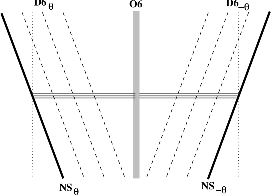
FIG. 41.: $N=1$ SQCD with orthogonal and symplectic groups can be realized using rotated NS fivebranes near an orientifold sixplane.

The moduli space of vacua can be studied by combining the discussion of section IV C 2 of orientifolds in theories with $N=2$ SUSY, and the results of this section on the reduction to $N=1$. We leave the details to the reader.

One can also analyze Seiberg’s duality for these systems by exchanging fivebranes and orientifolds in $x^{6}$. In the absence of orientifolds a quick way to find the dual is to exchange the branes while requiring the conservation of the linking number (111). The linking number for fivebranes near an orientifold sixplane is also given by (111) with the understanding that an $O6_{\pm}$ plane contributes to $L_{NS}$ like $\pm 2$ $D6$-branes. Using this, it is not difficult to show that the electric configuration of Fig. 41 is connected by duality to a magnetic one with gauge group $SO(\bar{N}_{c})$ with $\bar{N}_{c}=N_{f}-N_{c}+4$ for $O6_{+}$, and $Sp(\bar{N}_{c}/2)$ with $\bar{N}_{c}=N_{f}-N_{c}-4$ for $O6_{-}$.

If the rotation angle $\theta$ above is tuned to $\theta=\pi/2$, the fivebrane and its mirror image turn into $NS5^{\prime}$-branes and become parallel to the orientifold. The resulting SYM theory on the fourbranes is an $SO(N_{c})$ gauge theory with $2N_{f}$ chiral superfields in the vector representation, a chiral superfield $S$ in the symmetric representation and $W=0$. Motions of $D4$-branes along the $NS5^{\prime}$-brane (in $w$) correspond to expectation values of $S$ which parametrize an $N_{c}$ dimensional moduli space along which $SO(N_{c})$ is generically completely broken. Reversing the charge of the orientifold replaces $SO(N_{c})\rightarrow Sp(N_{c}/2)$ and $S\rightarrow A$, with $A$ a chiral multiplet in the antisymmetric tensor representation of $Sp(N_{c}/2)$.

The last two models are direct analogs of the $SU(N_{c})$ theory with an adjoint, fundamentals and $W=0$, discussed in subsection V B 4, with the symmetric of an orthogonal group ($S$) or antisymmetric of a symplectic group ($A$) playing the role of the adjoint field $\Phi$. Just like there, one can turn on a polynomial superpotential for the (anti-) symmetric tensor. For example, for the case of an $SO(N_{c})$ gauge group this is obtained by studying the following configuration: $k$ coincident $NS5_{\theta}$-branes to the left (in $x^{6}$) of an $O6_{+}$ plane, connected to their mirror images (which are $k$ coincident $NS5_{-\theta}$-branes) by $N_{c}$ fourbranes, with $N_{f}$ sixbranes parallel to the $NS5_{\theta}$-branes placed between the fivebranes and the orientifold. The SYM on the fourbranes is an $SO(N_{c})$ gauge theory with $2N_{f}$ vectors, a symmetric flavor $S$ and

$$W\sim{\rm Tr}S^{k+1}$$ (260)

The magnetic theory in the brane picture is obtained by interchanging the $k$ fivebranes with their mirror images while preserving the linking number (111) [89]. The magnetic theory has $G_{m}=SO(k(2N_{f}+4)-N_{c})$, $2N_{f}$ magnetic quarks, magnetic mesons and an appropriate superpotential, in agreement with field theory [137].

2. Orientifold Fourplane

As for the $N=2$ SUSY case discussed in section IV C 2, the situation is less well understood than that for $O6$-planes, so we will be brief.

The basic configuration that describes $N=1$ SQCD with an orthogonal or symplectic gauge group and matter in the fundamental representation includes $N_{c}$ fourbranes stretched between an $NS5$ and an $NS5^{\prime}$-brane, with $D6$-branes between them; all objects are stuck on an $O4$-plane, although the $D6$ and $D4$-branes could leave it in pairs (see Fig. 42). As discussed in section IV C 2, the charge of the orientifold flips sign each time it passes through an NS fivebrane. If the charge between the $NS5$ and $NS5^{\prime}$-branes is positive the gauge group is $Sp(N_{c}/2)$; negative charge corresponds to $SO(N_{c})$. The moduli space of vacua can be analyzed as in section IV C 2; we will not describe the details here. The fully Higgsed branch for both signs of the orientifold plane is illustrated in Fig. 43.

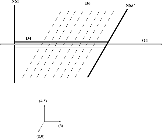
FIG. 42.: Branes near an $O4$-plane provide an alternative description of $N=1$ SYM theories with orthogonal and symplectic gauge groups.

To analyze the smooth transition that corresponds in brane dynamics to Seiberg’s duality we need to understand how to compute linking numbers in the presence of the $O4$-plane. Again, eq. (111) is essentially correct as long as we take into account the contributions of the $O4$-plane. An $O4_{\pm}$ plane contributes like $\pm 1$ $D4$-branes. Using this result, one can verify that Seiberg’s duality is reproduced in this system [87, 92, 89].

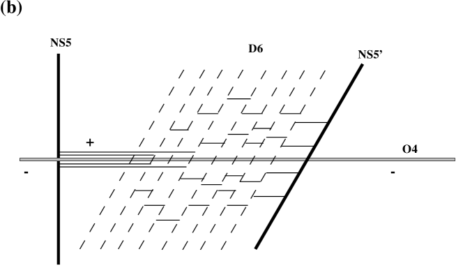
FIG. 43.: The fully Higgsed branch of moduli space corresponding to (a) $G=SO(4)$, and $N_{f}=8$ fundamentals; (b) $G=Sp(2)$, and $N_{f}=8$ fundamentals.

One can also study generalizations, e.g. replacing the single $NS5$-brane by $2k+1$ fivebranes leads to orthogonal and symplectic gauge theories with a massless adjoint field, with the polynomial superpotential $W\sim{\rm Tr}\Phi^{2(k+1)}$. Placing a sequence of $NS_{\theta}$-branes with different $\theta=\theta_{i}$ along the orientifold leads to theories with product gauge groups of the form $SO(k_{1})\times Sp(k_{2}/2)\times SO(k_{3})\times\cdots$ [219].

4 Unitary Gauge Groups With Two-Index Tensors

$N=1$ SYM theories with an $SU(N_{c})$ gauge group and chiral superfields in the (anti-) symmetric tensor representation can be constructed by starting with an $N=2$ configuration of branes near an $O6$-plane – mentioned at the end of subsection IV C 3 – and applying to it all the operations described in other cases. It is again sufficient to describe the theory for one sign of the orientifold charge (we will choose the case of positive sign). To get the theory corresponding to the other sign, one simply replaces symmetric tensors by antisymmetric ones, or vice-versa.

Consider an $NS5$-brane which is stuck on an $O6_{+}$ plane. An $NS5^{\prime}$-brane located to the left of the orientifold (in $x^{6}$) is connected to the $NS5$-brane by $N_{c}$ fourbranes. As usual, we place $N_{f}$ sixbranes between the fivebranes. The theory on the fourbranes is classically a $U(N_{c})$ gauge theory with $N_{f}$ fundamental flavors, two symmetric flavors $S$, $\tilde{S}$ and $W=0$. The analysis of the brane moduli space is easily seen to reproduce that of the proposed gauge theory. In particular, motions of the $D4$-branes in $w$, away from the $NS5$-brane, parametrize the $N_{c}$ dimensional moduli space of the theory along which $S$, $\tilde{S}$ get expectation values and the gauge group is typically completely broken. When all the fourbranes meet at a point in the $w$ plane that is not the position of the $NS5$-brane, an $SO(N_{c})$ gauge symmetry is restored and one recovers the theory with $G=SO(N_{c})$, a symmetric tensor, fundamentals and $W=0$, described in the previous subsection. Turning on the FI D-term in the $U(N_{c})$ theory (or entering the baryonic branch of the moduli space of the $SU(N_{c})$ one) has a similar effect.

Rotating the external $NS5^{\prime}$-brane to an $NS5_{\theta}$-brane, and at the same time rotating the $D6$-branes so that they are parallel to the $NS5_{\theta}$-branes, leads to a theory with the same matter content as before, but now with a classical superpotential for the symmetric tensor,

$$W\sim{1\over\mu}{\rm Tr}(S\tilde{S})^{2}$$ (261)

The previous case corresponds to $\mu=\infty$. Rearranging the branes leads to a dual configuration with gauge group $G_{m}=SU(3N_{f}+4-N_{c})$ and matter that can be easily analyzed as above. The resulting theory agrees with the field theory analysis [137].

If there are $k$ coincident $NS5_{\theta}$-branes outside the orientifold, one finds a similar theory but with (261) replaced by

$$W\sim{\rm Tr}(S\tilde{S})^{k+1}$$ (262)

Brane rearrangement leads to the Seiberg dual gauge group $SU((2k+1)N_{f}+4k-N_{c})$, again in agreement with field theory.

5 Chiral Models

Generic $N=1$ SYM theories are chiral. Such theories are interesting both because of their relevance to phenomenology and because of their rich dynamics. Their exploration using branes is in its infancy. Here we discuss a few families of brane configurations in the presence of orientifolds and orbifolds leading to chiral models that appeared in the recent literature.

The first family was studied in [161, 56, 90]. The brane configuration shown in Fig. 44 involves an $NS5^{\prime}$-brane which is embedded in an $O6$-plane, say at $x^{7}=0$. The $NS5^{\prime}$-brane divides the $O6$-plane into two disconnected regions, corresponding to positive and negative $x^{7}$. As we saw before, in this situation the RR charge of the orientifold jumps, from $+4$ to $-4$, as we cross the $NS5^{\prime}$-brane. The part of the orientifold with negative charge (which we will take to correspond to $x^{7}<0$) has furthermore eight semi-infinite $D6$-branes embedded in it. The presence of these $D6$-branes is required for charge conservation or, equivalently, vanishing of the six dimensional anomaly.

In addition to the eight semi-infinite $D6$-branes, we can place on the orientifold any number of parallel infinite $D6$-branes extending all the way from $x^{7}=-\infty$ to $x^{7}=\infty$. We will denote the number of such $D6$-branes by $2N_{f}$.

Then, an $NS_{\theta}$ fivebrane  located at a distance $L_{6}$ in the $x^{6}$ direction from the $NS5^{\prime}$-brane, but at the same value of $x^{7}$, is connected to the $NS5^{\prime}$-brane by $N_{c}$ $D4$-branes stretched in $x^{6}$. $N_{c}$ must be even for consistency. The mirror image of the $NS_{\theta}$-fivebrane, which is an $NS_{-\theta}$-fivebrane, is necessarily also connected to the $NS5^{\prime}$-brane.

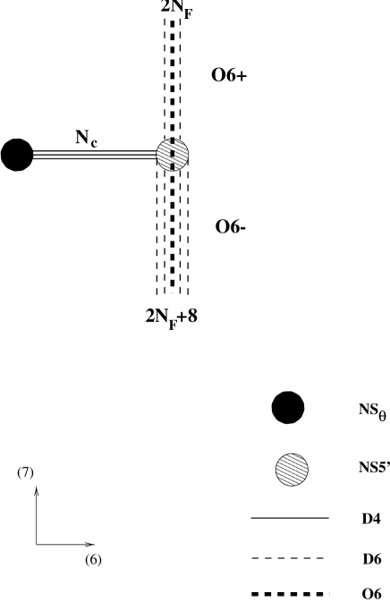
FIG. 44.: A chiral brane configuration in which an $NS5^{\prime}$-brane is stuck at an $O6$-plane and is connected to an $NS_{\theta}$-brane outside of the orientifold.

We can also place any number of $D6$-branes oriented at arbitrary angles $\theta_{i}$ (59) between the $NS_{\theta}$ fivebrane and the orientifold (in $x^{6}$). We will mainly discuss the case where such branes are absent, but it is easy to incorporate them.

We will next describe the gauge theory described by the above brane configuration. Before studying the general case we describe the structure for $\theta=0$ (when the external $NS_{\pm\theta}$-fivebranes are $NS5$-branes), and $\theta=\pi/2$ (when they are $NS5^{\prime}$-branes). We will only state the result, referring the reader to [90] for further discussion and derivations.

1. The Case $\theta=0$

The theory on the $D4$-branes has classical gauge group $U(N_{c})$ with a symmetric tensor $\tilde{S}$, an antisymmetric tensor $A$, $2N_{f}+8$ quarks $Q$ in the fundamental representation and $2N_{f}$ quarks $\tilde{Q}$ in the antifundamental representation. The superpotential is:

$$W=Q\tilde{S}Q+\tilde{Q}A\tilde{Q}$$ (263)

Fundamental chiral multiplets of the gauge group come from $4-6$ strings connecting the $D4$-branes to $D6$-branes ending on the $NS5^{\prime}$-brane from below (in $x^{7}$), while antifundamentals arise from $D6$-branes ending on the $NS5^{\prime}$-brane from above. The global symmetry of the system is determined by the gauge symmetry on the $D6$-branes, $Sp(N_{f})\times SO(2N_{f}+8)$. The superpotential (263) is the unique one consistent with this symmetry.

The theory is chiral and potentially anomalous as there are eight more fundamental than antifundamental chiral multiplets. The superpotential (263) implies that the symmetric tensor $\tilde{S}$ is in fact a symmetric bar (i.e. a symmetric tensor with two antifundamental indices). Thus the total anomaly $(2N_{f}+8)-2N_{f}+(N_{c}-4)-(N_{c}+4)$ vanishes, as one would expect for a consistent vacuum of string theory.

As a further check on the identification of the brane configuration and the chiral gauge theory one can analyze the moduli space of vacua as a function of various parameters one can add to the Lagrangian. An example is the FI D-term, which from the brane point of view corresponds to displacements in $x^{7}$ of the $NS5$-brane relative to the $NS5^{\prime}$-brane. In the gauge theory, adding to the Lagrangian a FI D-term for the $U(1)$ vectormultiplet ${\rm Tr}V$, $r\int d^{4}\theta\,{\rm Tr}V$, modifies the D flatness vacuum conditions:

$$AA^{\dagger}-\tilde{S}\tilde{S}^{\dagger}+QQ^{\dagger}-\tilde{Q}\tilde{Q}^{\dagger}=-r$$ (264)

Setting the quarks $Q$, $\tilde{Q}$ to zero we see that when $r$ is positive, $S$ gets an expectation value which breaks $U(N_{c})\to SO(N_{c})$. Due to the superpotential (263) the $2N_{f}+8$ chiral multiplets $Q^{i}$ as well as $\tilde{S}$ become massive and one if left with the $N=2$ spectrum and interactions for gauge group $SO(N_{c})$, with the antisymmetric tensor $A$ playing the role of the adjoint of $SO(N_{c})$. All of this is easily read off the brane configuration. In particular, the fact that the $2N_{f}+8$ quarks $Q^{i}$ are massive is due to the fact that the corresponding $4-6$ strings have finite length (proportional to $r$).

Similarly, for negative $r$ (264) implies that $A$ gets an expectation value, breaking $U(N_{c})$ to $Sp(N_{c}/2)$. The quarks $\tilde{Q}$ get a mass and we end up with an $N=2$ gauge theory with $G=Sp(N_{c}/2)$ and $2N_{f}+8$ light quarks.

2. The Case $\theta=\pi/2$

In this case the external fivebrane and its mirror image are $NS5^{\prime}$-branes. In addition to the matter discussed for the previous case there is now an adjoint field $\Phi$ parametrizing fluctuations of the fourbranes in the $w$ plane. The classical superpotential is:

$$W={\rm Tr}\tilde{S}\Phi A+Q\tilde{S}Q+\tilde{Q}A\tilde{Q}$$ (265)

As a check on the gauge theory we can again study the D-term perturbation corresponding to relative displacement in $x^{7}$ of the $NS5^{\prime}$-branes. For positive $r$ we now find an $SO(N_{c})$ gauge theory with $2N_{f}$ fundamental chiral multiplets, a symmetric tensor and vanishing superpotential. This can be understood by analyzing the D-flatness conditions (264) in the presence of the superpotential (265). As before, the symmetric tensor $\tilde{S}$ gets an expectation value, which for unbroken $SO(N_{c})$ must be proportional to the identity matrix. The first term in the superpotential (265) then gives rise to the mass term $W\sim\Phi A$. Since $A$ is antisymmetric, this term gives a mass to the antisymmetric part of $\Phi$ (as well as to $A$). The symmetric part of $\Phi$ becomes the symmetric tensor mentioned above. Clearly, it does not couple to the $2N_{f}$ fundamental chiral multiplets. In the brane description the fact that fluctuations of the fourbranes in $w$ are described by a symmetric tensor is a direct consequence of the action of the orientifold projection [108].

3. The General Case

For generic rotation angle $\theta$ (59) the adjoint field $\Phi$ discussed in the previous point is massive. Its mass $\mu(\theta)$ varies smoothly between zero at $\theta=\pi/2$ and $\infty$ for $\theta=0$. The superpotential describing this system is

$$W=Q\tilde{S}Q+\tilde{Q}A\tilde{Q}+\Phi A\tilde{S}+\mu(\theta)\Phi^{2}$$ (266)

For non-zero $\mu$ we can integrate $\Phi$ out and find the superpotential

$$W=Q\tilde{S}Q+\tilde{Q}A\tilde{Q}+\frac{1}{\mu(\theta)}(A\tilde{S})^{2}$$ (267)

for the remaining degrees of freedom. When $\theta\to 0$, $\mu\to\infty$, and (267) approaches (263). When $\theta=\frac{\pi}{2}$, the mass $\mu$ vanishes and it is inconsistent to integrate $\Phi$ out.

For generic $\theta$ none of the NS fivebranes in the configuration are parallel, and one can interchange them to find a dual magnetic theory. The magnetic gauge group one finds is $U(2N_{f}+4-N_{c})$. A careful field theory analysis leads to the same conclusion [90].

A second family of chiral models was studied by [164]. It has a gauge group which is a product of unitary groups with matter in the bifundamental of different pairs. It is obtained from brane configurations in $Z_{n}$ orbifold backgrounds in the following way. Start with $nN_{c}$ fourbranes stretched between two $NS5$-branes. The low energy theory on the fourbranes is $N=2$ SYM with gauge group $G=SU(nN_{c})$. We now mod out by the $Z_{n}$ symmetry acting on $v$ and $w$ as

$$(v,w)\to(v\exp(2\pi i/n),w\exp(-2\pi i/n))$$ (268)

Orbifolding breaks half of the supercharges and leads to an $N=1$ SUSY gauge theory with gauge group $SU(N_{c})_{1}\times SU(N_{c})_{2}\times SU(N_{c})_{3}\times\cdots\times SU(N_{c})_{n}$ with matter fields $F_{i}$, $i=1,...,n$, in the bifundamental $({\bf N}_{c},{\bf\bar{N}}_{c})$ of $SU(N_{c})_{i}\times SU(N_{c})_{i+1}$ (where $SU(N_{c})_{n+1}\equiv SU(N_{c})_{1}$). This theory is chiral for $n>2$. The curve describing its moduli space was obtained by [164].

An interesting variant of this theory is obtained by stretching $nN_{C}$ $D4$-branes between an $NS5$-brane and $n$ rotated fivebranes located at

$$v=\mu w,\quad v=\mu e^{4\pi i\over n}w,\quad v=\mu e^{8\pi i\over n}w,\quad\cdots\quad v=\mu e^{4(n-1)\pi i\over n}w$$ (269)

(of course these fivebranes are identified after orbifolding by (268), and so really describe a single fivebrane on $R^{4}/Z_{n}$). After modding out by the $Z_{n}$ group (268) one finds a gauge theory that is similar to that described above, but with a tree level superpotential

$$W=\mu{\rm Tr}F_{1}\cdots F_{n}$$ (270)

This superpotential lifts the moduli space, in agreement with the brane picture where for $\mu\neq 0$ the fourbranes are stuck at $v=w=0$. Adding $nN_{f}$ sixbranes and interchanging the $NS5$-brane with the $n$ rotated fivebranes leads to a magnetic $SU(N_{f}-N_{c})^{n}$ dual gauge theory.

A third class of models was also studied by [165]. It corresponds to webs of branes in the presence of orientifold planes and orbifold fixed points. As an example, one can start with the configuration of Fig. 19, that was shown in subsection IV C 2 to describe $SO$ or $Sp$ theories with $N=2$ SUSY (depending on the sign of the orientifold charge), and then mods out by the $Z_{3}$ symmetry (268) with $n=3$. The resulting gauge group is either $SO(N+4)\times SU(N)$ or $Sp(M)\times SU(2M+4)$, with matter in the following representations. For the first case (an $SO\times SU$ gauge group) there is an antisymmetric tensor field $A$ in the ${\bf{1\over 2}N(N-1)}$ of $SU(N)$ (it is a singlet under $SO(N+4)$), a field $\bar{Q}$ in the bifundamental $({\bf N+4,\overline{N}})$ of $SO(N+4)\times SU(N)$, and fundamentals of both groups, whose number is partly constrained by anomaly cancellation. The second case (an $Sp(M)\times SU(2M+4)$ gauge group) is related to the first one by replacing the antisymmetric tensor $A$ by a symmetric one $S$ but is otherwise similar.

The theories obtained this way have a vanishing superpotential. Rotating one of the $NS5$-branes in a way compatible both with the $Z_{2}$ orientifold projection and the $Z_{3}$ orbifold one, as in (269) (with $n=3$), leads to the appearance of a superpotential of the form $W\sim(\bar{Q}A\bar{Q})^{2}$ or $W\sim(\bar{Q}S\bar{Q})^{2}$ for the two cases. In the presence of a superpotential one can study $N=1$ duality, recovering results first obtained in field theory by [137].

VI Three Dimensional Theories

So far in this review we have focused on brane configurations realizing four dimensional physics, however, it is clear that the framework naturally describes field theory dynamics in different dimensions. In the remainder of the review we will study some brane configurations describing field theories in two, three, five and six dimensions.

We will see that these theories exhibit many interesting phenomena which can be studied using branes. Apart from the intrinsic interest in strongly coupled dynamics of various field theories in different dimensions and its realization in string theory, the main reason for including this discussion here is that it adds to the “big picture” and, in particular, emphasizes the generality and importance of:

1. “Universality:” one of the interesting features of the four dimensional analysis was the fact that understanding a few local properties of branes allowed the study of a wide variety of models with various matter contents and numbers of supersymmetries. These were obtained by combining branes in different ways in a sort of flat space “geometric engineering.” We will in fact see that this universality may allow one to understand  in a uniform way theories in different dimensions. This should be contrasted with the situation in field theory where the physics is described in terms of perturbations of weakly coupled fixed points, whose nature depends strongly on the dimensionality.

2. Hidden relations between different theories: in section III we saw how viewing a brane configuration from different points of view provides a relation between gauge theories in different dimensions with different amounts of SUSY. In that case, a relation between four dimensional $N=4$ SYM and two dimensional $N=(4,4)$ SYM provided an explanation of Nahm’s construction of multi-monopole moduli space. In this and the next two sections we will see that this is an example of a much more general phenomenon.

In this section we discuss three dimensional field theories, starting with the case of eight supercharges ($N=4$ SUSY), followed by four supercharges ($N=2$ SUSY). In the next two sections we discuss five, six and two dimensional theories. The presentation is more condensed than in the four dimensional case above. We only explain the basic phenomena in the simplest examples, referring the reader to the original papers for more extensive discussion.

A $N=4$ SUSY

The main purpose of this subsection is to describe the explanation using branes of two interesting field theory phenomena:

1. The Coulomb branch of a three dimensional $N=4$ SUSY gauge theory is often identical to the moduli space of monopoles in a different gauge theory.

2. Three dimensional $N=4$ SUSY gauge theories often have “mirror partners” such that the Higgs branch of one theory is the Coulomb branch of its mirror partner and vice-versa.

To study three dimensional gauge dynamics we consider, following [123], configurations of $D3$-branes suspended between $NS5$-branes in the presence of $D5$-branes. Using eqs. (8, 24, 26) it is not difficult to check that any combination of two or more of the following objects

$$\begin{array}[]{ll}\mbox{$NS5:$}&\mbox{$(x^{0},x^{1},x^{2},x^{3},x^{4},x^{5})$}\\ \mbox{$D3:$}&\mbox{$(x^{0},x^{1},x^{2},x^{6})$}\\ \mbox{$D5:$}&\mbox{$(x^{0},x^{1},x^{2},x^{7},x^{8},x^{9})$}\end{array}$$ (271)

in type IIB string theory preserves eight of the thirty two supercharges, and gives rise to an $N=4$ SUSY theory in the $1+2$ dimensional spacetime common to all branes $(x^{0},x^{1},x^{2})$. One can think of the branes (271) as obtained from (105) by performing T-duality in $x^{3}$.

As a first example, consider a configuration containing $k$ $D3$-branes stretched between two $NS5$-branes separated by a distance $L_{6}$ in $x^{6}$. As discussed at length above, the low energy theory on the threebranes is a three dimensional $N=4$ SUSY gauge theory with gauge group $G=U(k)$ and no additional light matter. The three dimensional gauge coupling is

$${1\over g^{2}}={L_{6}\over g_{s}}$$ (272)

Motions of the $k$ threebranes along the $NS5$-branes in $(x^{3},x^{4},x^{5})$ together with the duals of the $k$ photons, corresponding to the Cartan subalgebra of $G$, parametrize the $4k$ dimensional Coulomb branch of the $N=4$ SUSY gauge theory ${\cal M}_{k}$. Relative displacements of the two $NS5$-branes in $(x^{7},x^{8},x^{9})$ are interpreted as in (112) as FI D-terms. Note that the theory under consideration here can be thought of as a dimensional reduction of four dimensional $N=2$ SYM, or six dimensional $N=1$ SYM, in both cases without hypermultiplets, and thus much of the discussion of section IV C 1 applies to it. The $R$-symmetry, which is $SU(2)_{R}$ in six dimensions and $SU(2)_{R}\times U(1)$ in four dimensions, is enhanced by the reduction to three dimensions to $SU(2)_{R}\times SU(2)_{R^{\prime}}$, where $SU(2)_{R^{\prime}}$ acts as an $SO(3)$ rotation symmetry on $(x^{3},x^{4},x^{5})$.

From the point of view of the theory on the fivebranes, the $4k$ dimensional moduli space of BPS saturated deformations of the brane configuration ${\cal M}_{k}$ has a rather different interpretation. The situation is very similar to that discussed in section III. The worldvolume theory on the fivebranes is a gauge theory with $N=(1,1)$ SUSY (sixteen supercharges) and gauge group $G=U(2)$, broken down to $U(1)\times U(1)$ by an expectation value of one of the worldvolume scalars on the IIB fivebrane discussed in section II. This expectation value is proportional to the separation of the fivebranes $L_{6}$.

The massive $SU(2)$ gauge bosons correspond to D-strings connecting the two $NS5$-branes. $D3$-branes stretched between the $NS5$-branes are magnetic $SU(2)$ monopoles charged with respect to the unbroken $U(1)\subset SU(2)$ (the other $U(1)$ corresponding to joint motion of the fivebranes does not play a role and will be ignored below). In compact space they are U-dual to D-strings stretched between $D3$-branes, which were shown in section III to describe monopoles in a broken $SU(2)$ gauge theory. The $4k$ dimensional moduli space of brane configurations ${\cal M}_{k}$ is, from the point of view of the fivebrane theory, the moduli space of $k$ monopoles.

Thus we learn that the two spaces in question – the Coulomb branch of $N=4$ SUSY $U(k)$ gauge theory in $2+1$ dimensions and the moduli space of $k$ monopoles in $SU(2)$ gauge theory broken to $U(1)$ – are closely related; both are equivalent to the moduli space of SUSY brane configurations of Fig. 9. The $U(1)\subset U(k)$ corresponding to the center of mass of the $k$ monopole system gives rise to a trivial $R^{3}\times S^{1}$ part of the moduli space. The space of vacua of the remaining $SU(k)$ gauge theory corresponds to the moduli space of centered monopoles.

A closer inspection reveals that the two spaces related above are actually not identical; rather they provide descriptions of the moduli space of brane configurations in two different limits, which we describe next.

As we saw before, to study gauge physics using branes one needs to consider a limit in which gravity and massive string modes decouple. The relevant limit in this case is

$$L_{6},l_{s},g_{s}\rightarrow 0$$ (273)

with $L_{6}/g_{s}$ (272) held fixed.

From the point of view of the theory on the threebrane, the typical energy scale is set by the Higgs expectation values parametrizing the Coulomb branch. These are related using eq. (9) to the relative displacements of the threebranes along the fivebranes $\delta x$ by $\langle\phi\rangle\sim\delta x/l_{s}^{2}$. Thus, the typical distances between the threebranes in the gauge theory limit are

$$\delta x\sim\left({l_{s}^{2}g_{s}\over L_{6}^{2}}\right)L_{6}$$ (274)

To have a reliable $2+1$ dimensional picture one would like to require $\delta x\ll L_{6}$, i.e.:

$$Y\equiv\left({l_{s}\over L_{6}}\right)^{2}g_{s}\ll 1$$ (275)

The parameter $Y$ is clearly arbitrary in the limit (273) and when it satisfies (273, 275) the brane configuration is well described by $2+1$ dimensional field theory.

The scale (274) is natural from the point of view of the fivebrane theory as well. The (massive) charged $W$ bosons correspond to D-strings stretched between the two $NS5$-branes. Their mass is:

$$M_{W}={L_{6}\over g_{s}l_{s}^{2}}$$ (276)

The magnetic monopoles are much heavier. The gauge coupling of the $5+1$ dimensional fivebrane theory is (27) $g_{SYM}^{2}=l_{s}^{2}$; thus the effective coupling in the $1+3$ dimensional spacetime $(x^{0},x^{3},x^{4},x^{5})$ is

$${1\over g^{2}}={V_{12}\over l_{s}^{2}}$$ (277)

where $V_{12}$ is the volume of the $(x^{1},x^{2})$ plane which is eventually taken to infinity. Magnetic monopoles have mass

$$M_{\rm mon}\simeq{M_{W}\over g^{2}}={L_{6}V_{12}\over g_{s}l_{s}^{4}}$$ (278)

in agreement with their interpretation as $D3$-branes stretched between the $NS5$-branes. Recall that the size of a magnetic monopole is $\simeq M_{W}^{-1}$, much larger than its Compton wavelength $M_{\rm mon}^{-1}$ for weak coupling.

Thus we see that the scale $\delta x$ (274) is nothing but the Compton wavelength of a charged $W$ boson (276) or, equivalently, the size of a magnetic monopole. The five dimensional description as the moduli space of monopoles is appropriate when the scale of $SU(2)$ breaking $M_{W}$ (276) is much smaller than the scale of Kaluza-Klein excitations of the strings and threebranes stretched between fivebranes $1/L_{6}$. Requiring $M_{W}\ll 1/L_{6}$ leads to the constraint

$$Y\gg 1$$ (279)

on the parameter $Y$ defined in eq. (275). This is the opposite limit from that in which the $2+1$ dimensional picture is valid (275).

We see that rather than being identical, the three and five dimensional descriptions of the brane configuration are appropriate in different limits. As $Y\to 0$ the description of the space of vacua as the Coulomb branch of a three dimensional $SU(k)$ gauge theory becomes better and better, while as $Y\to\infty$ the five dimensional description becomes the appropriate one.

The dependence of the metric on $Y$ has not been analyzed. Presumably, as in other cases considered in previous sections, SUSY ensures that the metric on ${\cal M}_{k}$ does not depend on $Y$ and, therefore, its form for large $Y$ (where it is interpreted as the metric on the moduli space of $k$ monopoles) and for small $Y$ (where it is thought of as the metric on the Coulomb branch of a $d=2+1$, $N=4$ SUSY $SU(k)$ gauge theory) must coincide. It would be interesting to make this more precise.

The relation between monopoles and vacua of $2+1$ dimensional field theories can be generalized in many directions. To study monopoles in higher rank gauge theories we can consider, as in section IV C 3, chains of $NS5$-branes connected by $D3$-branes. For example, the configuration of Fig. 22 with the $D4$-branes (105) replaced by $D3$-branes (271) and no $D5$-branes ($d_{\beta}=0$) describes monopoles in broken $U(n+1)$ gauge theory. The monopoles carry charges under the $n$ unbroken $U(1)$’s in $SU(n+1)$. In a natural basis the magnetic charge of the configuration is $(k_{1},k_{2}-k_{1},k_{3}-k_{2},\cdots,k_{n}-k_{n-1},-k_{n})$.

From the point of view of the threebranes the configuration describes a $2+1$ gauge theory with gauge group $G=U(k_{1})\times U(k_{2})\times\cdots\times U(k_{n})$ with hypermultiplets transforming in the bifundamental representation of adjacent factors in the gauge group, $(k_{\alpha},\bar{k}_{\alpha+1})$ of $U(k_{\alpha})\times U(k_{\alpha+1})$ ($\alpha=1,\cdots,n-1$). The moduli space of vacua of this gauge theory is identical to the space of monopoles in broken $SU(n+1)$ gauge theory as discussed above.

The second field theory phenomenon that we would like to understand using branes is mirror symmetry [140], which was studied in string theory and M-theory in [65, 192, 123, 112, 68]. As pointed out by Hanany and Witten, this symmetry is a manifestation of the S-duality of the underlying $9+1$ dimensional IIB string theory. We will next illustrate the general idea in an example.

$N=4$ supersymmetric gauge theory with $G_{e}=U(N_{c})$ and $N_{f}$ hypermultiplets in the fundamental representation of the gauge group can be studied as in section IV. We consider $N_{c}$ $D3$-branes stretched between two $NS5$-branes, in the presence of $N_{f}$ $D5$-branes placed between the $NS5$-branes. All branes are oriented as in (271).

This theory has, like its four dimensional $N=2$ SUSY analog, a rich phase structure of mixed Higgs-Coulomb phases which can be studied classically as in section IV.

Under S-duality , the $NS5$-branes are exchanged with the $D5$-branes while the $D3$-branes remain invariant. The original configuration is replaced by one where $N_{c}$ $D3$-branes are stretched between two $D5$-branes with $N_{f}$ $NS5$-branes located between the two $D5$-branes (see Fig. 45).

This is a configuration that is by now familar. To exhibit the gauge group we have to reconnect threebranes stretched between the two $D5$-branes into pieces connecting $D5$-branes and $NS5$-branes, and other pieces connecting different $NS5$-branes. In doing that one has to take into account the s-rule, which implies that the $N_{c}$ threebranes attached to say the left $D5$-brane have to end on different $NS5$-branes. Thus if we break the first threebrane on the leftmost $NS5$-brane we have to break the second on the second leftmost, etc. A similar constraint has to be taken into account on the right $D5$-brane.

FIG. 45.: S-duality of IIB string theory implies mirror symmetry of the three dimensional $N=4$ SYM on $D3$-branes.

The maximal gauge symmetry one can obtain depends on $N_{f}$, $N_{c}$. The analysis is simplest for $N_{f}\geq 2N_{c}$ and we will describe only this case here. The generalization to $N_{f}<2N_{c}$ is simple.

Breaking the $N_{c}$ threebranes on the $NS5$-branes in the most general way consistent with the s-rule leads in this case to a magnetic gauge theory with $G_{m}=U(1)\times U(2)\times\cdots U(N_{c}-1)\times U(N_{c})^{N_{f}-2N_{c}+1}\times U(N_{c}-1)\times\cdots U(2)\times U(1)$. To see the hypermultiplets, it is convenient to move the left $D5$-brane past the leftmost $N_{c}$ $NS5$-branes (to which it is connected) and similarly for the right $D5$-brane.

The hypermultiplets can now be read off the brane configuration (Fig. 45(c)). They transform under $G_{m}$ as: $(1,2)\oplus(2,\bar{3})\oplus\cdots\oplus(k-1,\bar{k})\oplus k\oplus(k,\bar{k})\oplus\cdots\oplus(k,\bar{k})\oplus k\oplus(k,\overline{k-1})\oplus\cdots\oplus(3,2)\oplus(2,1)$.

The original electric brane configuration at a certain $g_{s}$ must, by S-duality, describe identical physics to the magnetic one at $\tilde{g}_{s}=1/g_{s}$ (but the same value of $l_{10}=l_{s}g_{s}^{1/4}$; see after eq. (55)). In the low energy limit $E\ll 1/l_{10}$ the electric configuration reduces to the electric gauge theory with gauge group $G_{e}$, while the magnetic one reduces to the magnetic gauge theory with gauge group $G_{m}$ (and the specified matter). Thus the two theories are clearly closely related.

However, as before, to go from one to the other, one has to tune a parameter describing the brane configuration to rather different values. In the electric theory the energy scale we want to hold fixed as we take $l_{10}\to 0$ is set by the three dimensional gauge coupling (272). To ignore Kaluza-Klein excitations on the threebranes, we must require $g_{s}/L_{6}\ll 1/L_{6}$, i.e. $g_{s}\ll 1$. Similarly, in the magnetic theory we must have $\tilde{g}_{s}\ll 1$ to be able to ignore Kaluza-Klein excitations.

When $g_{s}$ is small, there exists an energy scale for which all the complications of string theory can be neglected and the running gauge coupling of the electric gauge theory is still very small, so that we are in the vicinity of the UV fixed point of the gauge theory. The physics of the brane configuration below this energy is well described by gauge theory. Similarly, the magnetic gauge theory provides a good description of the low energy behavior of the brane configuration for large $g_{s}$ (or small $\tilde{g}_{s}$).

To relate the two gauge theories we must go to strong coupling $g_{s}\simeq 1$. In this regime the brane configuration is still described in the infrared by the same fixed point, but there is no longer an energy range in which it is well approximated by the full RG trajectory of either the electric or magnetic gauge theories. The KK excitations of the threebranes modify the RG flow at energies above $1/L_{6}\simeq g^{2}$, and one would expect the correspondence between the two gauge theories to break down.

In effect, the brane construction provides a deformation of the RG trajectories of both the electric and magnetic gauge theories that flow to the same IR fixed point, but with different UV behavior. In particular, the three dimensional dynamics is embedded in a four dimensional setting; the fourth (compact) dimension decouples in the extreme infrared but cannot be ignored at finite energies or for large Higgs expectation values. Thus, the brane construction shows that the low energy behavior of the electric and magnetic theories is identical in the strong coupling limit $g\to\infty$; equivalently, it shows that the infrared limits of the two models coincide for Higgs expectation values $\langle\phi\rangle\ll g^{2}$.

In gauge theory, mirror symmetry maps the Coulomb branch of the electric theory to the Higgs branch of the magnetic one and vice-versa. It also exchanges mass perturbations with FI D-terms. All this is manifest in the brane construction. As should be familiar by now, the Coulomb branch is described by motions of threebranes suspended between $NS5$-branes, while the Higgs branch corresponds to motions of threebranes stretched between $D5$-branes. Since under S-duality $NS5$-branes are exchanged with $D5$-branes, the Coulomb branch is exchanged with the Higgs branch. In the example discussed in detail above, it is not difficult to check that the (complex) dimensions of the electric Coulomb and Higgs branches are $N_{c}$ and $2N_{c}(N_{f}-N_{c})$, respectively, while in the magnetic theory they are reversed.

Similarly, since masses correspond in the brane language to relative displacements of $D5$-branes and FI D-terms are described by relative displacements of $NS5$-branes, S-duality permutes the two.

B $N=2$ SUSY

In this subsection we will study three dimensional $N=2$ SQCD. We start with a summary of field theoretic results followed by the brane description.

1 Field Theory

Consider $N=2$ SQCD with gauge group $G=U(N_{c})$ and $N_{f}$ flavors of chiral multiplets $Q^{i}$, $\tilde{Q}_{i}$ ($i=1,\cdots,N_{f}$) in the fundamental representation of $G$. This theory can be obtained from $N=1$ SQCD in four dimensions by dropping the dependence of all fields on $x^{3}$. The vector multiplet (83) gives rise upon reduction to three dimensions to a gauge field, a real scalar field in the adjoint representation of $G$, $X\equiv A_{3}$, and fermions. The chiral multiplets $(Q,\tilde{Q})$ reduce in an obvious way. The four dimensional gauge interaction (88) leads in three dimensions to a potential for the bosonic components of $Q$, $\tilde{Q}$

$$V\sim\sum_{i}|XQ^{i}|^{2}+|X\tilde{Q}_{i}|^{2}$$ (280)

More generally, one can compactify $x^{3}$ on a circle of radius $R$ and interpolate smoothly between four dimensional $(R\to\infty)$ and three dimensional $(R\to 0)$ physics. The three and four dimensional gauge couplings are related (classically) by $1/g_{3}^{2}=R/g_{4}^{2}$. Below, we describe the vacuum structure of the theory as a function of $R$.

The classical theory has an $N_{c}$ complex dimensional Coulomb branch. At generic points in the classical Coulomb branch the light degrees of freedom are the $N_{c}$ photons and scalars in the Cartan subalgebra of $U(N_{c})$, $A_{\mu}^{ii}$ and $X^{ii}$ $(i=1,\cdots,N_{c})$. Dualizing the photons

$$\partial_{\mu}\gamma^{ii}=\epsilon_{\mu\nu}^{\lambda}\partial^{\nu}A^{ii}_{\lambda}$$ (281)

gives rise to a second set of scalar fields $\gamma^{ii}$ which together with $X^{ii}$ form $N_{c}$ complex chiral superfields whose bosonic components are

$$\Phi^{j}=X^{jj}+i\gamma^{jj}$$ (282)

The expectation values of $\Phi^{j}$ parametrize the classical Coulomb branch.

In the three dimensional limit $R=0$ the scalars $\Phi^{j}$ live on a cylinder $R\times S^{1}$. $X^{jj}$ are non-compact, while $\gamma^{jj}$ live on a circle of radius $g_{3}^{2}$. For finite $R$, $\Phi^{j}$ live on a torus since then ${\rm Re}\Phi^{j}$ also live on a circle of radius $1/R$. In the four dimensional limit $R\to\infty$, holding the four dimensional gauge coupling fixed, the torus shrinks to zero size and the Coulomb branch disappears. The quarks are generically massive on the Coulomb branch (280).

For $N_{f}\geq N_{c}$ the theory has a $2N_{c}N_{f}-N_{c}^{2}$ dimensional Higgs branch with completely broken gauge symmetry (whose structure is the same as in four dimensions and, in particular, independent of $R$). There are also mixed Higgs-Coulomb branches corresponding to partially broken gauge symmetry.

In addition to the complex mass terms, described by a quadratic superpotential $W=m\tilde{Q}Q$, upon compactification to three dimensions one can write a “real mass” term for the quarks

$$\int d^{4}\theta Q^{\dagger}e^{m_{r}\theta\bar{\theta}}Q$$ (283)

We have encountered these real mass terms before: in the previous section, where we saw that the mass parameters in brane configurations describing three dimensional $N=4$ SUSY gauge theories have three components, and in (280), which describes a real mass term for the quarks proportional to $\langle X\rangle$.

Quantum mechanically, the gauge coupling is a relevant (=super-renormalizable) perturbation and thus the theory is strongly coupled in the infrared. Most or all of the Coulomb branch and in some cases part of the Higgs branch are typically lifted by strong coupling quantum effects. We next turn to a brief description of these effects as a function of $N_{f}$. A more detailed discussion appears in [3, 8, 69].

1. ${\bf N_{f}=0}$

The dynamics of $U(1)\subset U(N_{c})$ is trivial in this case since there are no fields charged under it. It gives a decoupled factor $R\times S^{1}$ in the quantum moduli space corresponding to $(1/N_{c})\sum\Phi^{j}$ (282). The $SU(N_{c})$ dynamics is non-trivial. A non-perturbative superpotential is generated by instantons, which in three dimensions are the familiar monopoles of broken $SU(N_{c})$ gauge theory. By using the symmetries of the gauge theory and the results of [228, 2] (for a review see [139] and references therein) for $N_{c}=2$ one can compute this superpotential exactly.

Any point in the Coulomb branch can be mapped by a Weyl transformation to the Weyl chamber $X^{11}\geq X^{22}\geq\cdots\geq X^{N_{c}N_{c}}$. In this wedge the natural variables are 

$$Y_{j}=\exp\left({\Phi^{j}-\Phi^{j+1}\over g_{3}^{2}}\right);\;\;\;j=1,\cdots,N_{c}-1$$ (284)

and one can show that the exact superpotential is

$$W=\sum_{j=1}^{N_{c}-1}{1\over Y_{j}}$$ (285)

This theory has no stable vacuum. The superpotential (285) tends to push the moduli $\Phi^{i}$ away from each other to infinity.

When the radius of compactification from four to three dimensions $R$ is non-zero the analysis is modified. The exact superpotential for finite $R$ is

$$W=\sum_{j=1}^{N_{c}-1}{1\over Y_{j}}+\eta\prod_{j=1}^{N_{c}-1}Y_{j}$$ (286)

where $\eta$ is related to the four dimensional QCD scale $\Lambda_{4}$:

$$\eta\sim\exp\left(-{1\over Rg_{3}^{2}}\right)\sim\exp\left(-{1\over g_{4}^{2}}\right)\sim\Lambda_{4}^{3N_{c}-N_{f}}$$ (287)

As $R\to 0$ at fixed $g_{3}$, $\eta\to 0$, while in the four dimensional limit ($R\to\infty$) $\eta$ turns into an appropriate power of the QCD scale (287).

The superpotential (286) is stable. Vacua satisfy $\partial_{j}W=0$ which leads to:

$$Z^{N_{c}}\eta^{N_{c}-1}=1;\;\;\;Z\equiv\prod_{i=1}^{N_{c}-1}Y_{i}$$ (288)

Thus, for all $R\not=0$ there are $N_{c}$ vacua corresponding to different phases of $Z$. As $R\to 0$, the vacua (288) recede to infinity. Since $\eta$ remains finite as $R\to\infty$, the $N_{c}$ solutions persist in the four dimensional limit.

As we add light fundamentals $Q$, $\tilde{Q}$, the vacuum structure becomes more intricate due to the appearance of Higgs branches and additional parameters such as real and complex masses, and FI D-terms. As in four dimensions, already classically there is a difference between $N_{f}\geq N_{c}$ and $N_{f}<N_{c}$ massless fundamentals – in the former case the gauge group can be broken completely, while in the latter the maximal breaking is $U(N_{c})\to U(N_{c}-N_{f})$. We next turn to the quantum structure in the two cases.

2. ${\bf N_{f}\leq N_{c}}$

The theory with $N_{f}=N_{c}$ and vanishing real masses at finite $R$ is described at low energies by a sigma model for $N_{c}^{2}+2$ chiral superfields $V_{\pm}$, $M^{i}_{\tilde{i}}$, with the superpotential

$$W=V_{+}V_{-}(\det M+\eta)$$ (289)

$M$ should be thought of as representing the meson field $M^{i}_{\tilde{i}}=Q^{i}\tilde{Q}_{\tilde{i}}$, $V_{\pm}$ parametrize the Coulomb branch and $\eta$ is given by (287). Note that most of the classical $N_{c}$ complex dimensional Coulomb branch is lifted in the quantum theory; its only remnants are $V_{\pm}$. The description (289) is arrived at by a combination of holomorphicity arguments, analysis of low $N_{c}$ and inspired guesswork which we will not review here (see [8]).

Varying (289) w.r.t. the fields $V_{\pm}$, $M$ gives rise to the equations of motion

$$V_{\pm}(\det M+\eta)=0;\;\;V_{+}V_{-}(\det M)(M^{-1})_{i}^{\tilde{i}}=0$$ (290)

Consider first the three dimensional case ($R=\eta=0$). There are three branches of moduli space:

1. $V_{+}=V_{-}=0$; $M$ arbitrary.

2. $V_{+}V_{-}=0$; $M$ has rank at most $N_{c}-1$.

3. $V_{+}$, $V_{-}$ arbitrary; $M$ has rank at most $N_{c}-2$.

The first branch can be thought of as a Higgs branch, while the last two are mixed Higgs-Coulomb branches. The three branches meet on a complex hyperplane on which the rank of $M$ is $N_{c}-2$ and $V_{+}=V_{-}=0$.

The understanding of the theory with $N_{f}=N_{c}$ allows us to study models with any $N_{f}\leq N_{c}$ by adding masses to some of the flavors and integrating them out. Adding a complex quark mass term $W=-mM$ to (289), the following structure emerges. If the rank of $m$ is one, one finds in the IR a theory with $N_{f}-1=N_{c}-1$ massless flavors. Integrating out the massive flavor one finds a moduli space of vacua with

$$V_{+}V_{-}\det M=1$$ (291)

where $M$ is the $(N_{f}-1)\times(N_{f}-1)$ matrix of classically massless mesons. Equation (291) implies that the classically separate Coulomb and Higgs branches merge quantum mechanically into one smooth moduli space. If the rank of $m$ is larger than one, one finds a superpotential with a runaway behavior. For example, if we add two non-vanishing masses:

$$W=V_{+}V_{-}\det M-m_{1}^{1}M^{1}_{1}-m_{2}^{2}M^{2}_{2}$$ (292)

we find, after integrating out the massive mesons $M_{1}^{i}$, $M_{j}^{1}$, $M_{2}^{i}$, $M_{j}^{2}$:

$$W=-{m_{1}^{1}m_{2}^{2}\over V_{+}V_{-}\det M}$$ (293)

where, again, $M$ represents the $(N_{f}-2)^{2}$ classically massless mesons. Clearly, the superpotential (293) does not have a minimum at finite values of the fields; there is no stable vacuum.

For a mass matrix $m$ of rank $N_{f}$

$$W=V_{+}V_{-}\det M-m_{i}^{\tilde{i}}M^{i}_{\tilde{i}}$$ (294)

we make contact with the case $N_{f}=0$. Integrating out the massive meson fields $M$ gives rise to the superpotential

$$W=-(N_{f}-1)\left({\det m\over V_{+}V_{-}}\right)^{1\over N_{f}-1}$$ (295)

This superpotential can be obtained from (285) by integrating out the $Y_{j}$ keeping $Z$ (288), and identifying it with $Z=V_{+}V_{-}$.

When the radius of the circle is not strictly zero ($\eta\not=0$), the analysis of (290) changes somewhat. There are now only two branches:

1. $V_{+}=V_{-}=0$; $M$ arbitrary.

2. $V_{+}V_{-}=0$; $\det M=-\eta$.

In particular, there is no analog of the third branch of the three dimensional problem. The two branches meet on a complex hyperplane on which $\det M=-\eta$ and $V_{+}=V_{-}=0$. The structure for all $\eta\not=0$ agrees with the four dimensional analysis of section V.

If we add to (289) a complex mass term $W=-mM$ with a mass matrix $m$ whose rank is smaller than $N_{f}$, the vacuum is destabilized (including the case of a mass matrix of rank one where previously there was a stable vacuum). If the rank of $m$ is $N_{f}$, so that the low energy theory is pure $U(N_{c})$ SYM, there are $N_{c}(=N_{f})$ isolated vacua which run off to infinity as the radius of the circle $R$ goes to zero (there is also a decoupled moduli space for the $U(1)$ piece of the gauge group). All this can be seen by adding to (295) the term proportional to $Z$, $\eta V_{+}V_{-}=\eta Z$, and looking for extrema of the superpotential

$$W=-(N_{f}-1)Z^{-{1\over N_{f}-1}}+\eta Z$$ (296)

We next turn to the dependence of long distance physics on the real masses of the quarks. As we saw before, real mass terms are described by D-terms (283); therefore, the effective low energy superpotential (289) is independent of these terms.

The effect of the real masses is to make some of the low energy degrees of freedom in (289) massive. To see that, consider weakly gauging the (vector) $SU(N_{f})$ flavor symmetry of (289). The real mass matrix $m_{i}^{\tilde{i}}$ corresponds to the expectation values of the scalars in the $SU(N_{f})$ vectormultiplet. A term analogous to (280) in the Lagrangian of the $SU(N_{f})$ theory will make some of the components of $M$ massive. For a diagonal mass matrix

$$\left(m_{r}\right)={\rm diag}\left(m_{1},m_{2},\cdots,m_{N_{f}}\right)$$ (297)

the off-diagonal components $M^{i}_{\tilde{i}}$ get a mass proportional to $|m_{i}-m_{\tilde{i}}|$. When all the real masses $m_{i}$ are different, the low energy limit is described by a sigma model for the $N_{f}+2$ fields $V_{+},V_{-},M_{1}^{1},M_{2}^{2},\cdots,M_{N_{f}}^{N_{f}}$ with the superpotential (compare to (289)),

$$W=V_{+}V_{-}\left(M_{1}^{1}M_{2}^{2}\cdots M_{N_{f}}^{N_{f}}+\eta\right)$$ (298)

More generally, if

$$\left(m\right)={\rm diag}\left(m_{1}^{n_{1}},m_{2}^{n_{2}},\cdots,m_{k}^{n_{k}}\right)$$ (299)

where $\{n_{i}\}$ are the degeneracies of $m_{i}$ and $\sum_{i}n_{i}=N_{f}$, the low energy limit includes $V_{\pm}$ and $k$ matrices $M_{i}$ whose size is $n_{i}\times n_{i}$ $(i=1,\cdots,k)$. The corresponding superpotential is

$$W=V_{+}V_{-}\left(\det M_{1}\det M_{2}\cdots\det M_{k}+\eta\right)$$ (300)

The moduli space corresponding to (300) is rather complicated in general. We have discussed the case of equal real masses $k=1$ before. We will next describe the other extreme case, $k=N_{f}$, leaving the general analysis to the reader.

In the three dimensional limit $\eta\to 0$, (298) describes $N_{f}+2\choose 2$ branches in each of which two of the $N_{f}+2$ fields $\{V_{\pm},M_{i}^{i}\}$ vanish. For non-zero $R$ (or $\eta$), there are three branches:

1. $V_{\pm}=0$; $M^{i}_{i}$ arbitrary.

2. $V_{+}=0$, $V_{-}\not=0$; $\prod_{i=1}^{N_{f}}M_{i}^{i}=\eta$.

3. $V_{-}=0$, $V_{+}\not=0$; $\prod_{i=1}^{N_{f}}M_{i}^{i}=\eta$.

3. ${\bf N_{f}>N_{c}}$

In this case, there is no (known) description of the low energy physics in terms of a sigma model without gauge fields. For vanishing real masses, instanton corrections again lift all but a two dimensional subspace of the Coulomb branch, which can be parametrized, as before, by two chiral superfields $V_{\pm}$. The Higgs branch is similar to that of the four dimensional theory; it is parametrized by the meson fields $M^{i}_{\tilde{i}}=Q^{i}\tilde{Q}_{\tilde{i}}$ subject to the classical compositness constraints (such that only $2N_{f}N_{c}-N_{c}^{2}$ of the $N_{f}^{2}$ components of $M$ are independent). An attempt to write a superpotential for $V_{+},V_{-}$ and $M^{i}_{\tilde{i}}$ using holomorphicity and global symmetries leads in this case to

$$W=\left(V_{+}V_{-}\det M\right)^{1\over N_{f}-N_{c}+1}$$ (301)

which is singular at the origin, clearly indicating that additional degrees of freedom that have been ignored become massless there.

For non-vanishing real masses the phase structure becomes quite intricate, and has not been analyzed using gauge theory methods. We will see later using brane techniques that when all the real masses are different there are $2N_{f}-N_{c}+2\choose N_{c}$, $N_{c}$-dimensional mixed Higgs-Coulomb branches intersecting on lower dimensional manifolds.

There are at least two other theories that have the same infrared limit as $N=2$ SQCD. One is the “mirror,” which just like for $N=4$ SYM is easiest to describe using branes [87, 70]; we will do this later. The other is the “Seiberg dual” [144, 4] which we will also describe using branes below. This is a gauge theory with $G_{m}=U(N_{f}-N_{c})$, $N_{f}$ flavors of magnetic quarks $q_{i}$, $\tilde{q}^{\tilde{i}}$, and singlet fields $M^{i}_{\tilde{i}}$, $V_{\pm}$ which couple to the magnetic gauge theory via the superpotential

$$W=M^{i}_{\tilde{i}}q_{i}\tilde{q}^{\tilde{i}}+V_{+}\tilde{V}_{-}+V_{-}\tilde{V}_{+}$$ (302)

where $\tilde{V}_{\pm}$ are the effective fields parametrizing the unlifted quantum Coulomb branch of the magnetic gauge theory.

It should be emphasized that the three dimensional “Seiberg duality” is different from its four dimensional analog in at least two respects. The first is that it is not really a strong-weak coupling duality. In three dimensions both the electric and magnetic descriptions are strongly coupled (with the exception of the case $N_{f}=N_{c}>1$ where the superpotential (289) is dangerously irrelevant and, therefore, the sigma model is weakly coupled in the IR, at least at the origin of moduli space). Thus it is less useful as a tool to study strong coupling dynamics.

The second is that the magnetic theory is not well formulated throughout its RG trajectory. In particular, the fields $\tilde{V}_{\pm}$ are effective low energy degrees of freedom that emerge after taking into account non-perturbative gauge dynamics. They are ill defined in the high energy limit in which the magnetic theory is (asymptotically) free.

Of course, the equivalence of the electric and magnetic theories is expected to hold only in the IR, so this is not necessarily a problem for the duality hypothesis. However, it does seem to suggest that the three dimensional Seiberg duality is a low energy manifestation of a relation between different theories that reduce to low energy SYM in the IR but have quite different high energy properties. We will next argue that the relevant theories are theories on branes.

2 Brane Theory

To study four dimensional $N=1$ SQCD compactified on a circle of radius $R$ using branes [89] we can simply compactify the corresponding type IIA configuration (i.e. take $x^{3}\sim x^{3}+2\pi R$ in Fig. 24). At large $R$ we recover the results of section V. For small $R$ it is convenient to perform a T-duality on the $x^{3}$ circle; this transforms type IIA to IIB and turns $D4$-branes wrapped around $x^{3}$ into $D3$-branes at points on the dual circle of radius

$$R_{3}={l_{s}^{2}\over R}$$ (303)

The $NS5$ and $NS5^{\prime}$-branes transform to themselves, while the $D6$-branes turn into $D5$-branes at points in $(x^{3},x^{4},x^{5},x^{6})$. We will mostly use the IIB language to describe the physics.

FIG. 46.: The brane realization of mirror symmetry in three dimensional $N=2$ SYM.

The IIB brane configuration corresponding to three dimensional $N=2$ SQCD is depicted in Fig. 46. The classical analysis of deformations and moduli mirrors closely the discussion of section V. Compactification to three dimensions gives rise to a new branch of moduli space – the Coulomb branch, and new parameters in the Lagrangian – the real masses. The former correspond in the brane language to locations in $x^{3}$ of $D3$-branes stretched between the $NS5$ and $NS5^{\prime}$-branes. The latter are given by the positions in $x^{3}$ of the $N_{f}$ $D5$-branes.

Note that due to (303), as $R_{3}\to\infty$ we recover the three dimensional $N=2$ SQCD theory with $\eta=0$ which was discussed in the previous subsection, while the four dimensional limit corresponds to $R_{3}\to 0$. The three dimensional gauge coupling is given in type IIB language by (272), $1/g_{3}^{2}=L_{6}/g_{s}$. The four dimensional gauge coupling is related to it by $1/g_{3}^{2}=R/g_{4}^{2}$ or, using (303),

$${1\over g_{4}^{2}}={L_{6}R_{3}\over g_{s}l_{s}^{2}}$$ (304)

The gauge theory limit corresponds to (273). To get a three dimensional theory further requires $R_{3}\to\infty$ with $L_{6}/g_{s}$ held fixed; the four dimensional limit is $R_{3}\to 0$ with $g_{4}$ (304) held fixed. The instanton effects which give rise to the term proportional to $\exp(-1/g_{4}^{2})$ in (286) arise from Euclidean D-strings which are stretched between the $NS5$ and $NS5^{\prime}$-branes and are wrapped around the $x^{3}$ circle.

As discussed in the previous subsection, the infrared dynamics of the gauge theory in question has at least two alternative descriptions, the mirror and the Seiberg dual. Both are easy to understand using branes. To construct the mirror, we apply an S-duality transformation to the electric configuration; the result is described in Fig. 46(b). The $NS5$ and $NS5^{\prime}$-branes are exchanged with $D5$ and $D5^{\prime}$ branes, while $D3$-branes are invariant. The mirror brane configuration is very similar to that found for $N=4$ SQCD in the section VI A. The only difference is that one of the two $D5$-branes has been rotated into a $D5^{\prime}$-brane. $N=2$ mirror symmetry was suggested in [87] and further investigated in [70].

To find the gauge symmetry of the mirror theory we break the threebranes on the $NS5$-branes in the most general way (Fig. 46(b)). This leads to the gauge group $U(1)\times U(2)\times\cdots\times U(N_{c}-1)\times U(N_{c})^{N_{f}-N_{c}}$. There is still matter in bifundamental representations of adjacent factors of the gauge group, and since $D3$-branes stretched between $NS5$-branes actually preserve $N=4$ SUSY, there are also chiral multiplets transforming in the adjoint of each factor. The $D3$-branes stretched between the $D5^{\prime}$ brane and the closest $NS5$-brane give rise as usual to $N_{c}$ scalars $M_{\alpha}$ which couple via a cubic superpotential to $N_{c}$ fundamentals of the “last” $U(N_{c})$ factor. The analysis of the magnetic theory involves no new elements; details appear in [70].

The Seiberg dual is obtained as usual by exchanging fivebranes in $x^{6}$. Since the two NS fivebranes are not parallel, we expect the transition to be smooth and the resulting theory to be equivalent in the infrared to the original one. The magnetic brane configuration one is led to is in fact very similar to that obtained in the four dimensional case, with $D4$ and $D6$-branes replaced by $D3$ and $D5$-branes. In particular, classically it seems to correspond to a $G_{m}=U(N_{f}-N_{c})$ gauge theory with magnetic quarks and $N_{f}^{2}$ singlet mesons $M$ with the superpotential $W=Mq\tilde{q}$. Comparing to the gauge theory result (302), we seem to be missing the two fields $V_{\pm}$ and their couplings to the gauge degrees of freedom.

What saves the day is the fact that the equivalence between the electric and magnetic theories is expected to be a quantum feature, while our analysis of the magnetic brane configuration so far was purely classical. Thus our next task is to study the quantum vacuum structure corresponding to the electric and magnetic brane configurations. We will first describe the structure for the electric theory and, in particular, reproduce the gauge theory results of the previous subsection. We will then turn to the magnetic theory and show that in fact the fields $V_{\pm}$ are secretly present in the three dimensional analog of Fig. 28 (but are not geometrical, like the adjoint field with a polynomial superpotential discussed in section V). We will also see evidence of the superpotential (302).

The tool we will use to analyze the vacuum structure is the quantum brane interaction rules described in section V C 3. As explained there, this allows one to analyze the moduli space for widely separated branes. The behavior for branes that are close to each other has to be addressed by other means. Unfortunately, the M-theory analysis is inapplicable for type IIB configurations and there are at present no known alternatives.

Consider the electric configuration of Fig. 46(a) with $N_{f}=0$. The $N_{c}$ threebranes stretched between the NS fivebranes repel each other; therefore, the classical $N_{c}$ dimensional Coulomb branch is lifted. The repulsive potential between pairs of adjacent threebranes can be thought of in this case as due to Euclidean D-strings stretched between the $NS5$ and $NS5^{\prime}$-branes and between the $D3$-branes (as in Fig. 34). They correspond to instantons in the low energy three dimensional gauge theory. Since there are two fermionic zero modes in the presence of these instantons, they lead to a superpotential on the classical Coulomb branch.

In the three dimensional theory (with $R_{3}=\infty$, or $\eta=0$ (287)), the long range repulsion between threebranes leads to runaway behavior, since there is no stable vacuum with the threebranes at finite distances; this is in agreement with the gauge theory analysis of the superpotential (285). For finite $R_{3}$ (or $\eta$) the threebranes arrange around the $x^{3}$ circle at equal spacings, maximizing the distances between them and leading to an isolated vacuum. The fact that there are $N_{c}$ vacua (288) has to do with the dual of the three dimensional gauge field (281, 282), and is not expected to be seen geometrically in the current setup. As $R_{3}\to\infty$ the vacua run off to infinity, and we recover the previous results.

In the presence of massless quarks, in the brane description there are $D5$-branes in the system that can “screen” the interactions between the threebranes. This screening can be seen directly by studying Euclidean D-strings stretched between $D3$-branes. If the worldsheet of such a D-string intersects a $D5$-brane, two additional zero modes appear and the contribution to the superprotential vanishes.

For $1\leq N_{f}\leq N_{c}-2$ massless flavors we saw before that the gauge theory is unstable and exhibits a runaway superpotential (given by (293) for $N_{f}=N_{c}-2$). In the brane picture we have $N_{c}$ threebranes stretched between $NS5$ and $NS5^{\prime}$-branes, and $N_{c}-2$ $D5$-branes located at the same value of $x^{3}$ (we are restricting to the case of vanishing real masses for now) between the $NS5$ and $NS5^{\prime}$-branes.

Due to the repulsion between unscreened threebranes stretched between $NS5$ and $NS5^{\prime}$-branes, $N_{c}-2$ of the $N_{c}$ threebranes must break on different $D5$-branes. The s-rule implies that once this has occurred, no additional threebranes attached to the $NS5$-brane can break on these $D5$-branes. We are left with two unbroken threebranes, one on each side of the $D5$-branes (in $x^{3}$). These threebranes repel each other, as well as the pieces of the broken threebranes stretched between the $NS5^{\prime}$-brane and the $D5$-brane closest to it. There is no screening in this situation since all $N_{c}-2$ $D5$-branes are connected to the $NS5$-brane; hence they can be removed by moving them past the $NS5$-brane in $x^{6}$, using the HW transition. The system is unstable, and some or all of the threebranes mentioned above must run away to infinity.

This is in agreement with the gauge theory analysis of the superpotential (293). One can think of $V_{\pm}$ as the positions in $x^{3}$ of the two threebranes stretched between $NS5$ and $NS5^{\prime}$-branes mentioned above (as usual, together with the dual of the three dimensional gauge field). The potential obtained from (293) indeed suggests a repulsion between the different threebranes.

It is clear that the arguments above continue to hold when the radius of the circle on which the threebranes live is finite. While the two threebranes stretched between the $NS5$ and $NS5^{\prime}$-branes can no longer run away to infinity in the $x^{3}$ direction, those connecting the $NS5^{\prime}$-brane to a $D5$-brane (representing components of $M$) can, and there is still no stable vacuum. This is in agreement with gauge theory; adding the term $W=\eta V_{+}V_{-}$ to (293) and integrating out $V_{\pm}$ leads to a superpotential of the form $W\sim(\det M)^{-1/2}$.

The above discussion can be repeated with the same conclusions for all $1\leq N_{f}\leq N_{c}-2$.

For $N_{f}=N_{c}-1$ the gauge theory answer is different; there is still no vacuum in the four dimensional case $\eta\not=0$, while in three dimensions there is a quantum moduli space of vacua with $V_{+}V_{-}\det M=1$. In brane theory there are now $N_{c}-1$ $D5$-branes, and the interaction between the D threebranes stretched between $NS5$ and $NS5^{\prime}$-branes can be screened. Indeed, consider a situation where $N_{c}-2$ of the $N_{c}$ threebranes stretched between $NS5$ and $NS5^{\prime}$-branes break on $D5$-branes. This leaves two threebranes and one $D5$-brane that is not connected to the $NS5$-brane. If $R_{3}=\infty$ (i.e. $\eta=0$), the single $D5$-brane can screen the repulsion between the two threebranes. If the threebrane is at $x^{3}=0$, then using the rules of subsection V C 3 we deduce that any configuration where one of the threebranes is at $x^{3}>0$ while the other is at $x^{3}<0$ is stable. The locations in $x^{3}$ of the two threebranes give the two moduli $V_{\pm}$. Thus, the brane picture predicts correctly the existence of the quantum moduli space and its dimension. The precise shape of the moduli space (the relation $V_{+}V_{-}\det M=1$) is a feature of nearby branes and thus is expected to be more difficult to see; nevertheless, it is clear that due to the repulsion there is no vacuum when either $V_{+}$ or $V_{-}$ vanish.

If the radius of the fourth dimension $R$ is not zero, there is a qualitative change in the physics. Since $R_{3}$ is now finite, the two threebranes stretched between $NS5$ and $NS5^{\prime}$-branes are no longer screened by the $D5$-brane – they interact through the other side of the circle. Thus one of them has to break on the remaining $D5$-brane, and one remains unbroken because of the s-rule. The repulsion between that threebrane and the threebranes stretched between the $NS5^{\prime}$-brane and a $D5$-brane which is no longer screened leads to vacuum destabilization, in agreement with the gauge theory analysis.

For $N_{f}=N_{c}$ (and vanishing real masses) the brane theory analysis is similar to the previous cases, and the conclusions are again in agreement with gauge theory. For $R_{3}=\infty$ one finds three phases corresponding to a pure Higgs phase in which there are no threebranes stretched between $NS5$ and $NS5^{\prime}$-branes, and two mixed Higgs-Coulomb phases in which there are one or two threebranes stretched between the $NS5$ and $NS5^{\prime}$-branes; the locations of the threebranes in $x^{3}$ are parametrized by $V_{\pm}$. When there are two unbroken threebranes, they must be separated in $x^{3}$ by the $D5$-branes, which provide the necessary screening.

For finite $R_{3}$, the structure is similar, except for the absence of the branch with two unbroken threebranes, which is lifted by the same mechanism to that described in the case $N_{f}=N_{c}-1$ above. $N_{f}>N_{c}$ works in the same way as in the four dimensional case described earlier.

So far we discussed the electric theory with vanishing (more generally equal) real masses for the quarks. Turning on real masses gives rise to a rich phase structure of mixed Higgs-Coulomb branches. We have seen an example in the theory with $N_{f}=N_{c}$. The three dimensional theory with $\eta=0$ and vanishing real masses, which is equivalent in the infrared to the sigma model (289), has three branches described after equation (290). When all the real masses are different, the corresponding sigma model (298) has $(N_{f}+1)(N_{f}+2)/2$ $N_{f}$-dimensional branches intersecting on lower dimensional manifolds. For $N_{f}>N_{c}$ the problem has not been analyzed in gauge theory.

Branes provide a simple way of studying the phase structure. As an example we will describe it for the case of arbitrary $N_{f}\geq N_{c}$ with all $N_{f}$ real masses different. The generalization to cases where some of the real masses coincide is straightforward.

The brane configuration includes in this case $N_{f}$ $D5$-branes at different values of $x^{3}$. The $N_{c}$ $D3$-branes can either stretch between the $NS5$ and $NS5^{\prime}$-branes or split into two components on $D5$-branes. Different branches of moduli space correspond to different ways of distributing $D3$-branes between the two options, in such a way that there are no unscreened interactions.

Stability implies that any two $D3$-branes stretched between the $NS5$ and $NS5^{\prime}$-branes must be separated (in $x^{3}$) by a $D5$-brane that screens the repulsive interaction between them. Similarly, a $D3$-brane stretched between the $NS5$ and $NS5^{\prime}$-branes and a second one that is broken into two components on a $D5$-brane must be separated by such a $D5$-brane.

To describe the different branches of the quantum moduli space of vacua we have to place the $N_{c}$ $D3$-branes in such a way that there are no repulsive interactions. Each threebrane can either be placed between two $D5$-branes, or on top of one. There are therefore $N_{f}+(N_{f}+1)=2N_{f}+1$ possible locations for $D3$-branes corresponding to the $N_{f}$ $D5$-branes and the $N_{f}+1$ spaces between and around them. The quantum interactions between branes mean that one cannot place two threebranes at adjacent locations. The number of branches is, therefore, the number of ways to distribute $N_{c}$ identical objects between $2N_{f}+1$ slots, with at most one object per slot and no two objects sitting in adjacent slots. It is not difficult to show that this number is

$${n\choose k};\;\;n\equiv 2N_{f}-N_{c}+2,\;k\equiv N_{c}$$ (305)

We next turn to the magnetic brane configuration. Naively it describes a $U(\bar{N}_{c})$ gauge theory with $N_{f}$ fundamentals $q$, $\tilde{q}$, a magnetic meson $M$ and the standard superpotential

$$W=M\tilde{q}q$$ (306)

To see whether this is in fact correct we will study the resulting theory for the special case $\bar{N}_{c}=N_{f}$ and compare the vacuum structure of the gauge theory to that of the brane configuration, which is described by a three dimensional analog of Fig. 28. We will furthermore discuss only the three dimensional limit $\eta=0$. Classically, the two definitely agree. The theory has an $N_{f}^{2}+N_{f}$ dimensional moduli space of vacua; in the brane language it corresponds to independent motions of the color branes along the NS fivebranes and to breaking of flavor threebranes on different $D5$-branes. In gauge theory it is parametrized by expectation values of $M$ and the $\Phi^{j}$ (282). Quantum mechanically, one finds a discrepancy, which we describe next.

Before turning on the Yukawa superpotential (306), the low energy dynamics of the gauge theory in question is described by the sigma model (289) for the fields $\tilde{M}\equiv\tilde{q}q$ and $\tilde{V}_{\pm}$ which parametrize the potentially unlifted Coulomb branch of the theory. Coupling the “magnetic quarks” $q$, $\tilde{q}$ to the singlet meson $M$ leads to a low energy sigma model with the superpotential

$$W=\tilde{V}_{+}\tilde{V}_{-}\det\tilde{M}+M\tilde{M}$$ (307)

Varying with respect to $M$ sets $\tilde{M}=0$. Therefore, we conclude that the quantum gauge theory in question has a two complex dimensional moduli space of vacua parametrized by arbitrary expectation values of the fields $\tilde{V}_{\pm}$.

On the other hand the brane configuration has a unique vacuum at the origin where all $\bar{N}_{c}=N_{f}$ threebranes are aligned and can be thought of as stretching between the $NS5$-brane and the $N_{f}$ $D5$-branes. This is the only stable configuration, taking into account the repulsive interactions between color threebranes and the attractive interactions between color and flavor threebranes.

We conclude that the gauge theory leading to the low energy sigma model (307) cannot provide a full description of the physics of the brane configuration of Fig. 28. In [89] it is proposed that the magnetic brane configuration is in fact described by the above gauge theory, but there are two more fields $V_{\pm}$ that are singlets under the $U(\bar{N}_{c})$ gauge group and contribute the term

$$W_{V}=V_{+}\tilde{V}_{-}+V_{-}\tilde{V}_{+}$$ (308)

to the low energy superpotential. Combining (307) with (308) clearly gives the right quantum vacuum structure for $\bar{N}_{c}=N_{f}$, and also more generally. Note that the term (308) is just what has been seen to be needed in gauge theory to generalize Seiberg’s duality to three dimensions (302)! In particular, it can be used to make sense of the dual theory, which as we discussed in the previous subsection is not really well defined as a local quantum field theory. We see that the high energy theory that underlies (302) is best thought of as the theory on the web of branes described by the three dimensional Fig. 28.

The fields $V_{\pm}$ and their interactions (308) are not seen geometrically in the brane configuration. This makes it more difficult in general to compare the vacuum structure of three dimensional Seiberg duals. Nevertheless, in all cases that have been checked, no disagreement has been found, supporting the proposed duality. Some tests of the equivalence of the theories with vanishing real masses appear in [4]. We have further checked the other extreme case of $N_{f}$ different real masses in a few examples and find agreement. For $N_{f}=N_{c}$ the magnetic theory can be shown to reduce to the sigma model (289), or when all the real masses are different, (298). As we have seen above, the magnetic moduli space has in this case $(N_{f}+2)(N_{f}+1)/2$ branches, in agreement with the electric theory (305).

For $N_{f}=N_{c}+1$, the magnetic theory reduces in the infrared to a $U(1)$ gauge theory with $N_{f}$ flavors and the superpotential (302). By using the results of [8] one can check that the phase structure of the magnetic theory is again in agreement with (305). It would be interesting to check agreement for arbitrary $N_{f}>N_{c}$.

VII Two Dimensional Theories

A Field Theory Results

Two dimensional gauge theories with $N=(4,4)$ supersymmetry can be obtained by the dimensional reduction of six dimensional $N=(1,0)$ theories (or four dimensional $N=2$ theories). The $1+5$ dimensional Lorentz symmetry is broken to $SO(1,1)\times Spin(4)$ and the latter combines with the $R$-symmetry to a $Spin(4)\times SU(2)_{R}$ global symmetry group.

As in four dimensional $N=2$ theories, two dimensional $(4,4)$ gauge theories have two massless representations: a hypermultiplet and a vectormultiplet (also called a twisted multiplet). In terms of an $N=(2,2)$ superalgebra the hypermultiplets decompose into two chiral multiplets (see for example [232] for a review of two dimensional $N=(2,2)$ theories). The scalars in these multiplets parametrize a “Higgs branch ” which is a Hyper-Kähler manifold. The vectormultiplet decomposes into a chiral multiplet and a twisted chiral multiplet. The scalars in these superfields parametrize the “Coulomb branch,” which is characterized by a generalized Kähler potential determining the metric and torsion on target space [104].

Next we consider $U(1)$ gauge theories with $N_{f}$ “electron” hypermultiplets. The Coulomb branch is parametrized by the expectation values ${\vec{\phi}}\in R^{4}$ of the four scalars in the twisted multiplet. Classically, the metric on the Coulomb branch is flat. Quantum mechanically, the metric receives a contribution whose form is fixed by hyper-Kähler geometry, and whose normalization can be determined by an explicit one-loop computation. In the massless case the metric is [194]

$$ds^{2}=\left({1\over g_{2}^{2}}+{N_{f}\over\vec{\phi}^{2}}\right)d{\vec{\phi}}^{2}$$ (309)

where $g_{2}$ is the $2d$ gauge coupling. The coefficient in front of $d{\vec{\phi}}^{2}$ is the effective gauge coupling.

Turning on bare masses $\vec{m}_{i}$, $i=1,...,N_{f}$, to the hypermultiplets the metric becomes

$$ds^{2}=\left({1\over g_{2}^{2}}+\sum_{i=1}^{N_{f}}{1\over|\vec{\phi}-\vec{m}_{i}|^{2}}\right)d{\vec{\phi}}^{2}$$ (310)

One notes that this is precisely the form of the metric of a $2d$ CFT describing the propagation of a string near $N_{f}$ parallel NS fivebranes (22). We shall see in the next section that this is not an accident. Moreover, the torsion $H=dB$ on the Coulomb branch is also given by equation (22).

As in previous sections, it will also be interesting to consider a compactification, in this case from three to two dimensions on a circle of radius $R$. The Coulomb branch is four dimensional and is parametrized by the expectation values of the three scalars in the vector multiplet, $\vec{\rho}\in R^{3}$, and the scalar $\sigma$ dual to the $3d$ gauge field; $\sigma$ lives on a circle, $\sigma\sim\sigma+1/R$. The metric on the Coulomb branch now takes the form [74]

$$ds^{2}=2\pi R\left({1\over g_{3}^{2}}+\sum_{i=1}^{N_{f}}{1\over|\vec{\rho}-\vec{m}_{i}|}\Big{\{}{1\over 2}+\sum_{n=1}^{\infty}e^{-2\pi Rn|\vec{\rho}-\vec{m}_{i}|}\cos[2\pi Rn(\sigma-\sigma_{i})]\Big{\}}\right)(d{\vec{\rho}}^{2}+d\sigma^{2})$$ (311)

The coefficient in front of $d{\vec{\rho}}^{2}+d\sigma^{2}$ is the effective gauge coupling of a $3d$ theory compactified to $2d$ on $S^{1}_{R}$ and $g_{3}$ is the three dimensional coupling constant, which is related to the two dimensional coupling constant by standard dimensional reduction

$${1\over g_{2}^{2}}={2\pi R\over g_{3}^{2}}$$ (312)

When $R\to 0$ the metric (311) approaches (310) with $\vec{\phi}\equiv(\vec{\rho},\sigma)$. For large compactification radius, $R\gg 1/|\vec{\rho}|$, the effective gauge coupling becomes

$${1\over g_{2}^{2}}+\pi R\sum_{i=1}^{N_{f}}{1\over|\vec{\rho}-\vec{m}_{i}|}$$ (313)

This is similar to the metric (31) on an ALE space with a resolved $A_{N_{f}-1}$ singularity which appeared when we discussed the metric felt by a string in the presence of $N_{f}$ parallel KK monopoles. Again, as we shall discuss later, this is not an accident.

For $SU(2)\simeq Sp(1)$ gauge group with $N_{f}$ “quark” hypermultiplets, the metric on the Coulomb branch of the two dimensional $(4,4)$ theory is [74]

$$ds^{2}=\left({1\over g_{2}^{2}}+\sum_{i=1}^{N_{f}}\Big{\{}{1\over|\vec{\phi}-\vec{m}_{i}|^{2}}+{1\over|\vec{\phi}+\vec{m}_{i}|^{2}}\Big{\}}-{2\over\vec{\phi}^{2}}\right)d{\vec{\phi}}^{2}$$ (314)

This metric is related to an ALE space with a resolved $D_{N_{f}}$ singularity for reasons that we shall point out later.

Next we turn to $N=(2,2)$ supersymmetric gauge theories in two dimensions. $(2,2)$ SCFTs in $2d$ were studied, in particular, in the context of standard perturbative string compactifications since they lead to spacetime supersymmetric vacua. Here we shall only touch upon a small class of $(2,2)$ theories.

Two dimensional $N=(2,2)$ theories can be obtained by dimensional reduction of four dimensional $N=1$ supersymmetric theories. Since anomaly constraints are milder in $2d$, generic chiral, anomalous $4d$ gauge theories typically lead to consistent $2d$ theories. Therefore, we may consider gauged linear sigma models like a $U(N_{c})$ gauge theory with $n$ quarks $Q$ in the fundamental representation ${\bf N}_{c}$ and $\tilde{n}$ anti-quarks $\tilde{Q}$ in the anti-fundamental ${\bf\bar{N}}_{c}$, where $n$ is not necessarily equal to $\tilde{n}$ (for a recent review and further references on such theories see [120]). When $\tilde{n}=0$ and $N_{c}=1$ this is the $CP^{n-1}$ model. When $\tilde{n}=0$ and $N_{c}>1$ this theory is called the “Grassmanian model.” The space of its classical vacua is the complex Grassmanian manifold $G(N_{c},n)$. The dynamics of vacua of the sigma model with target space $G(N_{c},n)$ is described by the $U(N_{c})/U(N_{c})$ gauged WZW model with the level $k$ of $SU(N_{c})$ being

$$k=n-N_{c}$$ (315)

In this case there is a “level-rank duality” (see [172] and references therein) which exchanges:

$$N_{c}\leftrightarrow k$$ (316)

This duality is the stetement that the space of conformal blocks of an $SU(N_{c})$ WZW model at level $k$ is identical to the one of $SU(k)$ at level $N_{c}$ and, therefore, the topological theory $U(N_{c})/U(N_{c})$ at level $k$ is equivalent to the theory $U(k)/U(k)$ at level $N_{c}$.

B Brane Theory I: $(4,4)$ Theories

Two dimensional unitary gauge theories with $(4,4)$ supersymmetry appear on D-strings near $D5$-branes. In particular, the low energy theory on a $D1$-brane stretched in $(x^{0},x^{1})$ near $N_{f}$ parallel $D5$-branes stretched in $(x^{0},x^{1},x^{2},x^{3},x^{4},x^{5})$ is a $U(1)$ gauge theory with $N_{f}$ flavors. The metric on the Coulomb branch of the theory – parametrized by the location of the $D1$-brane in the four directions transverse to the $D5$-branes $l_{s}^{2}\vec{\phi}=(x^{6},x^{7},x^{8},x^{9})$ – should be equal to the background metric of a D-string in the presence of $N_{f}$ parallel $D5$-branes located at $l_{s}^{2}\vec{m}_{i}$, $i=1,...,N_{f}$. This type IIB system is $S$-dual to a fundamental string in the presence of $N_{f}$ parallel NS fivebranes. This explains the relation between the metric (310) (and torsion) on the Coulomb branch and those of a string propagating in the background of solitonic fivebranes (22).

Three dimensional gauge theories with eight supercharges compactified to two dimensions on $S^{1}_{R}$ can be studied on $D2$-branes stretched in $(x^{0},x^{1},x^{6})$) near $N_{f}$ $D6$-branes stretched in $(x^{0},x^{1},x^{2},x^{3},x^{4},x^{5},x^{6})$, both wrapping a circle of radius $R$ in the $x^{6}$ direction. Consider a single $D2$-brane. $T_{6}$-duality (51) maps it to a $D1$-brane near $N_{f}$ $D5$-branes at points on a transverse circle of radius

$$R_{6}=l_{s}^{2}/R$$ (317)

The background metric of a fivebrane transverse to a circle in the $x^{6}$ direction and located, say, at $(x^{6},x^{7},x^{8},x^{9})=0$ can be obtained by considering an infinite array of fivebranes separated by a distance $2\pi R_{6}$. It gives rise to an H-monopole background with metric and torsion given by [105]:

$$G_{IJ} = e^{2(\Phi-\Phi_{0})}\delta_{IJ};\qquad I,J,K,M=6,7,8,9$$ (318)

$$H_{IJK} = -\epsilon_{IJKM}\partial^{M}\Phi$$ (319)

$$e^{2(\Phi-\Phi_{0})}-1 = \sum_{n=-\infty}^{\infty}{l_{s}^{2}\over{\vec{x}}^{2}+(x^{6}-2\pi R_{6}n)^{2}}$$ (320)

$$= {l_{s}^{2}\over 2R_{6}x}\,{\sinh(x/R_{6})\over\cosh(x/R_{6})-\cos(x^{6}/R_{6})}$$ (321)

$$= {l_{s}^{2}\over 2R_{6}x}\Big{\{}1+\sum_{n=1}^{\infty}e^{-nx/R_{6}}\cos(nx^{6}/R_{6})\Big{\}}$$ (322)

where $x=|\vec{x}|$, $\vec{x}=(x^{7},x^{8},x^{9})$. From (317, 322) we see that the metric on the Coulomb branch (311) is precisely the metric of $N_{f}$ H-monopoles located at $(x^{6}_{i},\vec{x}_{i})=2\pi l_{s}^{2}(\sigma_{i},\vec{m}_{i})$, $i=1,...,N_{f}$. We thus see again how the geometry is probed by D-branes.

In the limit $R_{6}\to\infty$ we obtain a system of $N_{f}$ fivebranes in non-compact space which was discussed above. This is compatible with the fact that in this limit (322) behaves like $1/{\vec{\phi}}^{2}$, where $\vec{\phi}=(x^{6},\vec{x})/2\pi l_{s}^{2}$.

On the other hand, in the limit $R\to\infty$ we get on the $D2$-brane a $1+2$ dimensional $N=2$ SUSY $U(1)$ gauge theory with $N_{f}$ flavors. The background metric of the $D6$-branes should be related to the metric on the Coulomb branch of that gauge theory. As discussed in section II, $D6$-branes are KK monopoles in M-theory, and they are described by the same metric as KK monopoles in type IIA string theory. A KK monopole with charge $R/l_{s}$ (Taub-NUT) is related by T-duality (in an appropriate sense) to an H-monopole (322) for any value of $R$ [119]. In particular, when $R\to\infty$ (322) behaves like $R/|\vec{\rho}|$, where $\vec{\rho}=\vec{x}/2\pi l_{s}^{2}$, which is compatible with a Coulomb branch with effective coupling (313). Metrics similar to these showed up already in other (related) situations in this review, such as in sections III D and VI A.

A $(4,4)$ SUSY gauge theory in two dimensions with gauge group $Sp(1)\simeq SU(2)$ can be obtained on a $D1$-brane (and its mirror image) near an orientifold fiveplane parallel to $N_{f}$ $D5$-branes (and their $N_{f}$ mirror images). On a transverse circle of radius $R_{6}$ it describes a compactification from three to two dimensions on a circle of radius $R$ (317). T-duality in this transverse direction gives instead an $O6$-plane parallel to $2N_{f}$ $D6$-branes, whose background metric is related to an ALE space with resolved $D_{N_{f}}$ singularity [203, 210, 215]. T-dualizing back to the original system (and taking $R_{6}\to\infty$) gives rise to the metric (314) in agreement with $2d$ field theory.

An alternative way to study $(4,4)$ $2d$ theories on branes is to allow branes to end on branes, as in previous sections. A typical configuration involves $N_{c}$ $D2$-branes stretched between two $NS5$-branes, with $N_{f}$ $D4$-branes located between them (or, equivalently by an HW transition, $N_{f}$ $D4$-branes to the left (right) of the left (right) NS-brane, each connected to the NS-brane by a single $D2$-brane). This configuration is T-dual to configurations preserving eight supercharges which were studied in previous sections (Figs. 11,14). The branes involved here have worldvolumes

$$\begin{array}[]{ll}\mbox{$NS5:$}&\mbox{$(x^{0},x^{1},x^{2},x^{3},x^{4},x^{5})$}\\ \mbox{$D2:$}&\mbox{$(x^{0},x^{1},x^{6})$}\\ \mbox{$D4:$}&\mbox{$(x^{0},x^{1},x^{7},x^{8},x^{9})$}\end{array}$$ (323)

The low energy theory on the $D2$-branes is a $U(N_{c})$ gauge theory with $N_{f}$ quark flavors and classical gauge coupling

$${1\over g_{2}^{2}}={L_{6}l_{s}\over g_{s}}$$ (324)

where $L_{6}$ is the distance between the two NS-branes in $x^{6}$ (as before, we consider the limit $g_{s},l_{s}\to 0$ such that $g_{2}$ is held fixed). The locations of the $D2$-branes along the NS-branes $\vec{r}_{a}=(x^{2}_{a},x^{3}_{a},x^{4}_{a},x^{5}_{a})$, $a=1,...,N_{c}$, parametrize the Coulomb branch of the theory. The locations of the $D4$-branes $\vec{r}_{i}=(x^{2}_{i},x^{3}_{i},x^{4}_{i},x^{5}_{i})$, $i=1,...,N_{f}$, are the bare masses of quark hypermultiplets. Higgsing correspond to breaking $D2$-branes on $D4$-branes, and the relative motion of the two NS-branes in $(x^{7},x^{8},x^{9})$ corresponds to a FI D-term.

When $\vec{r}_{a}=\vec{r}_{i}=0$, the brane configuration is invariant under rotations in $(x^{2},x^{3},x^{4},x^{5})$ and $(x^{7},x^{8},x^{9})$. These $Spin(4)_{2345}$ and $SU(2)_{789}$ rotations, respectively, are associated with the global $R$-symmetries of the $(4,4)$ gauge theory.

The interpretation of the torsion on the Coulomb branch in the brane picture is the following [54]. A $D2$-brane ending on an NS fivebrane looks like a string in the $(2,0)$ six dimensional theory on the fivebrane. Strings in six dimensions couple to the self-dual two-form $B$, which is identified with the $2d$ $B$-field. Each fundamental hypermultiplet corresponds to a $D2$-brane ending on an NS-brane and contributes to the torsion.

Quantum mechanically, the NS-branes bend due to Coulomb-like interactions in four dimensions (61). For simplicity, we consider the $U(1)$ theory: a single $D2$-brane located at $\vec{r}$. As in previous sections, the resulting effective gauge coupling is given by the distance between the NS-branes in $x^{6}$ as a function of $\vec{r},\vec{r}_{i}$:

$${x^{6}l_{s}\over g_{s}}={1\over g_{eff}^{2}}={1\over g_{2}^{2}}+\sum_{i=1}^{N_{f}}{l_{s}^{4}\over|\vec{r}-\vec{r}_{i}|^{2}}$$ (325)

This is indeed the exact effective coupling in field theory (310) with $\vec{\phi}\equiv\vec{r}/l_{s}^{2}$, $\vec{m}_{i}\equiv\vec{r}_{i}/l_{s}^{2}$.

As usual, the type IIA configuration at finite $g_{s}$ is equivalent to M-theory on a compact circle of radius $R_{10}=g_{s}l_{s}$. The relative location of the “NS fivebranes” in $x^{10}$ correspond to a “$\theta$ angle.” This $\theta$ parameter together with the FI D-term – the relative position of the fivebranes in $(x^{7},x^{8},x^{9},x^{10})$ – combine into a “quaternionic Kähler form.”

In M-theory, the $SU(2)_{R}$ symmetry is enhanced to a $Spin(4)_{7,8,9,10}$. Indeed, [239] argues that this should happen in field theory. It thus seems from the brane picture that quantum mechanically there is a “mirror symmetry” interchanging masses with FI D-term and theta parameters, and the Coulomb branch with the Higgs branch. For more details we refer the reader to [54].

Brane configurations giving rise to three dimensional gauge theories compactified to two dimensions on a circle of radius $R$ can be studied using the above configurations by compactifying $x^{2}$ on a circle of radius $R_{2}=l_{s}^{2}/R$ (or their $T_{2}$-dual versions). In particular, the NS fivebranes now bend due to Coulomb-like forces in $R^{3}\times S^{1}$. The solution to Laplace equation in this case gives rise to a distance in $x^{6}$ which is compatible with the field theory effective gauge coupling given in (311).

Finally, we may add to the configurations above an orientifold twoplane (fourplane) parallel to the $D2$-branes ($D4$-branes) and obtain symplectic or orthogonal gauge groups in two dimensions. For example, considering two $D2$-branes stretched between the $NS5$-branes in the presence of an $O2$-plane, together with $2N_{f}$ $D4$-branes, gives rise to either an $SO(2)\simeq U(1)$ or $Sp(1)\simeq SU(2)$ gauge theory, depending on the sign of the orientifold charge. Taking into account the sign flip of the orientifold charge, and the Coulomb-like interactions associated with $D2$-branes, their mirror images and the $O2$-plane, gives rise to a bending of the $NS5$-branes which is in agreement with the field theory results (310) and (314):

$${x^{6}l_{s}\over g_{s}}={1\over g_{eff}^{2}}={1\over g_{2}^{2}}+\sum_{i=1}^{N_{f}}\Big{\{}{l_{s}^{4}\over|\vec{r}-\vec{r}_{i}|^{2}}+{l_{s}^{4}\over|\vec{r}+\vec{r}_{i}|^{2}}\Big{\}}-{(1+1)(1+1)l_{s}^{4}\over|2\vec{r}|^{2}}\pm{(1/2+1/2)l_{s}^{4}\over|\vec{r}|^{2}}$$ (326)

The second term on the right hand side of (326) is due to the $N_{f}$ flavors and their $N_{f}$ mirror images, the third term is due to a $D2$-brane at $\vec{r}$ having its mirror image at $-\vec{r}$, and the last term is due to the $O2$-plane – the “$\pm$” corresponding to orthogonal or symplectic projections, respectively. Obviously, this discussion can be generalized to other dimensions and to compactifications from high to lower dimensions performing the analysis with an orientifold charge and Coulomb-like interactions in the appropriate dimension .

Brane configurations corresponding to two dimensional $(4,4)$ gauge theories were also considered in [21, 141].

C Brane Theory II: $(2,2)$ Theories

We may now rotate branes in the configurations of the previous section and get at low energy two dimensional $N=(2,2)$ supersymmetric gauge theories on the $D2$-branes. As an example, we shall examine a configuration of an $NS5$-brane connected to an $NS5^{\prime}$-brane by $N_{c}$ $D2$-branes in the presence of $N_{f}$ $D4$-branes. The worldvolumes of the various objects are given in (323, 195).

FIG. 47.: $D4$-branes oriented as explained in the text can split into two disconnected components and separate along an NS fivebrane in $(x^{2},x^{3})$.

A new ingredient which appears in such a brane configuration is the possibility to put a $D4$-brane at the same $x^{6}$ location of the $NS5^{\prime}$-brane, then break it and separate the two semi-infinite pieces along the $NS5^{\prime}$-brane in the $\sigma$ direction:

$$\sigma\equiv x^{2}+ix^{3}$$ (327)

We may break all the $N_{f}$ $D4$-branes on the $NS5^{\prime}$-brane and take part of the semi-infinite $D4$-branes to infinity. One then obtains a configuration where, say, $n$ semi-infinite $D4$-branes – stretched in $x^{7}>0$ – are located at $\sigma_{i}$, $i=1,...,n$, along the $NS5^{\prime}$-brane, and $\tilde{n}$ semi-infinite $D4$-branes – stretched in $x^{7}<0$ – are located at $\sigma_{\tilde{i}}$, ${\tilde{i}}=1,...,{\tilde{n}}$ (see Fig 47).

The low energy theory on the $D2$-branes is a two dimensional $(2,2)$, $U(N_{c})$ gauge theory with $n$ quarks and $\tilde{n}$ anti-quarks. There is a manifest chiral flavor symmetry $U(n)\times U(\tilde{n})$ which is broken for generic values of $\sigma_{i}$, $\sigma_{\tilde{i}}$. One can check that the classical moduli space of vacua and deformations of the brane configuration (almost) agree with a field theory analysis [120].

In M-theory, the $NS5$-brane and $D4$-branes ending on the $NS5^{\prime}$-brane turn into two disconnected $M5$-branes. The type IIA $D2$-branes turn into $M2$-branes connecting these $M5$-branes. The dynamics of such open membranes stretched between two fivebranes is not completely understood; nevertheless, chiral features of the quantum $(2,2)$ theories can be studied in this way. We refer the reader to [120] for details.

We should remark that the Coulomb-like interactions associated with the $D4$-branes ending on the $NS5^{\prime}$-brane give rise to terms which are logarithmic in $\sigma$ and which contribute to the quantum low energy $2d$ effective superpotential. Logarithmic effective superpotentials are indeed familiar in such two dimensional $(2,2)$ theories (namely, in gauged linear sigma models). Other relations between the parameter space of $(2,2)$ theories in two dimensions and the moduli space of $N=2$ four dimensional theories – associated with the $D4$-branes ending on the $NS5^{\prime}$-brane – are discussed in [120].

Finally, let us consider a duality trajectory interchanging the $NS5$ and $NS5^{\prime}$-brane in the $x^{6}$ direction. The details of this process can be worked out along the lines of previous sections (up to an ambiguity which is resolved quantum mechanically in M-theory [120]). Here we shall only state the result in the case $\tilde{n}=0$, namely, for a $G(N_{c},n)$ model (see section VII A). The duality trajectory takes an electric $U(N_{c})$ theory with $n$ quarks to a magnetic $U(n-N_{c})$ theory with $n$ quarks, i.e.

$$G(N_{c},n)\leftrightarrow G(n-N_{c},n)$$ (328)

providing a brane realization of the level-rank duality (316, 315) discussed in section VII A.

VIII Five And Six Dimensional Theories

A Five Dimensional Field Theory Results

$N=1$ supersymmetric gauge theories in five dimensions have eight supercharges and an $SU(2)_{R}$ global symmetry. The two possible multiplets in the theory are the vectormultiplet in the adjoint of the gauge group $G$ – containing a vector field, a real scalar $\phi$ and fermions – and the hypermultiplet in a representation $R_{f}$ of $G$ – containing four real scalars and fermions. The Coulomb branch is parametrized by the scalar components of the vector multiplet $\phi^{i}$, $i=1,...,{\rm rank}G$, in the Cartan sub-algebra of $G$.

The low energy theory is determined by the prepotential ${\cal F}(\phi)$, which is required to be at most cubic due to $5d$ gauge invariance [204]. The exact quantum prepotential is given by [138]

$${\cal F}={1\over 2g_{0}^{2}}\phi^{i}\phi_{i}+{c_{cl}\over 6}d_{ijk}\phi^{i}\phi^{j}\phi^{k}+{1\over 12}\left(\sum_{\alpha}|\alpha_{i}\phi^{i}|^{3}-\sum_{f}\sum_{w\in R_{f}}|w_{i}\phi^{i}+m_{f}|^{3}\right)$$ (329)

Here $g_{0}$ is the bare coupling of the gauge theory and $d_{ijk}$ is the third rank symmetric tensor: $d_{abc}={\rm Tr}(T_{a}\{T_{b},T_{c}\})/2$. The first sum in (329) is over the roots of $G$ and the second sum is over the weights of the representation $R_{f}$ of $G$; $m_{f}$ are the (real) masses of the hypermultiplets in $R_{f}$. $c_{cl}$ is a quantized parameter of the theory, related to a $5d$ Chern-Simons term. In terms of ${\cal F}$ the effective gauge coupling is

$$\left({1\over g^{2}}\right)_{ij}={\partial^{2}{\cal F}\over\partial\phi^{i}\partial\phi^{j}}$$ (330)

From now on we discuss simple groups $G$ with $N_{f}$ hypermultiplets in the fundamental representation of $G$:

• $G=SU(N_{c})$ ($N_{c}>2$): The Coulomb branch of the moduli space is given by $\phi={\rm diag}(a_{1},...,a_{N_{c}})$ with $\sum_{i=1}^{N_{c}}a_{i}=0$. The prepotential in this case is

  $${\cal F}={1\over 2g_{0}^{2}}\sum_{i=1}^{N_{c}}a_{i}^{2}+{1\over 12}\left(2\sum_{i<j}^{N_{c}}|a_{i}-a_{j}|^{3}+2c_{cl}\sum_{i=1}^{N_{c}}a_{i}^{3}-\sum_{f=1}^{N_{f}}\sum_{i=1}^{N_{c}}|a_{i}+m_{f}|^{3}\right)$$ (331)

  The conditions on $N_{c}$, $N_{f}$ and $c_{cl}$ in (329) are

  $$c_{cl}+{1\over 2}N_{f}\in Z$$ (332)

  $$SU(N_{c}):\qquad N_{f}+2|c_{cl}|\leq 2N_{c}$$ (333)

• $G=SU(2)$: This case is somewhat special. There are two pure gauge theories labeled by a $Z_{2}$ valued theta angle, since $\pi_{4}(SU(2))=Z_{2}$. $c_{cl}$ is irrelevant since $d_{ijk}=0$ in (329), and the number of flavors allowed is $N_{f}\leq 7$.

• $G=SO(N_{c})$ $(Sp(N_{c}/2))$: In this case $c_{cl}=0$ and

  $$SO(N_{c})\,\,(Sp(N_{c}/2)):\qquad N_{f}\leq N_{c}-4\,\,(N_{f}\leq N_{c}+4)$$ (334)

  The inequalities in (333, 334) are necessary conditions to have non-trivial fixed points which one can use to define the $5d$ gauge theory.

In five dimensions there are no instanton corrections to the metric and, therefore, the exact results considered above are obtained already at one loop. However, compactifying the theory gives rise to non-perturbative corrections. Supersymmetric $5d$ gauge theories compactified to four dimensions on a circle were studied in [99, 177, 100, 178]. The perturbative contributions to ${\cal F}$ from KK modes were found, and were shown to obtain the correct behavior in the five and four dimensional limits. Non-perturbative corrections to ${\cal F}$ are conjectured to be related to spectral curves of relativistic Toda systems.

B Webs Of Fivebranes And Five Dimensional Theories

We begin by considering a $D5$-brane ending (classically) on an $NS5$-brane [7]. Recall (section II D) that type IIB fivebranes sit in a $(p,q)$ multiplet of the $SL(2,Z)$ S-duality group, where the $NS5$-brane is a $(0,1)$ fivebrane while the $D5$-brane is a $(1,0)$ fibebrane. We choose the worldvolumes of these fivebranes to be

$$\begin{array}[]{ll}\mbox{$NS5\,\,(0,1):$}&\mbox{$(x^{0},x^{1},x^{2},x^{3},x^{4},x^{5})$}\\ \mbox{$D5\,\,(1,0):$}&\mbox{$(x^{0},x^{1},x^{2},x^{3},x^{4},x^{6})$}\end{array}$$ (335)

Classically, we may let the $D5$-brane end on the NS fivebrane, say from the left in $x^{6}$. Such a configuration is allowed – as discussed in section II E 3 – and it is T-dual to situations where $D4$ or $D3$-branes are ending on NS fivebranes as in previous sections. Therefore, this configuration preserves eight supercharges.

Quantum mechanically the NS fivebrane bends. Its bending is due to the fact that the $D5$-brane ending on the NS fivebrane looks like an electric charge in one dimension. This causes a linear Coulomb-like interaction (see (61)) which leads to the bending of the $NS5$-brane in the $(x^{5},x^{6})$ plane into the location

$$x^{6}={g_{s}\over 2}(|x^{5}|+x^{5})$$ (336)

Here and below we set $a=0$ in the complex type IIB string coupling $\tau$ (44), for simplicity. Moreover, without lose of generality we chose the intersection of the fivebranes to be located at the origin $(x^{5},x^{6})=0$, and the extension of the $NS5$-brane to be as in (335) when $x^{5}<0$.

While we started classically from a semi-infinite fivebrane ending on an infinite fivebrane, what we have obtained instead – quantum mechanically – is an intersection of three semi-infinite fivebranes (Fig 48). All fivebranes share the same $1+4$ directions $(x^{0},x^{1},x^{2},x^{3},x^{4})$ and are real straight lines in the $(x^{5},x^{6})$ plane. In the example above we have three semi-infinite fivebranes meeting at the origin. The semi-infinite fivebrane located at $x^{6}=0$ and stretched along $x^{5}<0$ is the $NS5$-brane. The semi-infinite fivebrane located at $x^{5}=0$ and stretched along $x^{6}<0$ is the $D5$-brane. The third semi-infinite fivebrane is located (336) at $x^{6}=g_{s}x^{5}$, $x^{5},x^{6}>0$.

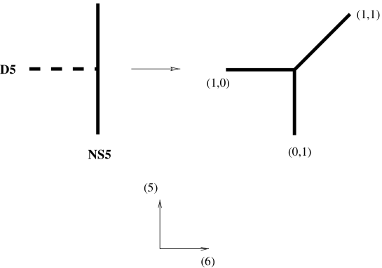
FIG. 48.: The classical configuration of a $D5$-brane ending on an NS fivebrane is replaced for finite $g_{s}$ by a vertex in which $(1,0)$ and $(0,1)$ fivebranes merge into a $(1,1)$ fivebrane.

Which is the fivebrane located at $x^{6}=g_{s}x^{5}$? Clearly, it is a $(1,1)$ fivebrane! Charge conservation does not really allow a $D5$-brane to end on an $NS5$-brane. Instead, at the intersection point the $(1,0)$ and $(0,1)$ fivebranes merge together to form a $(1,1)$ fivebrane. In order for this “new” $(1,1)$ fivebrane not to break supersymmetry any further, it must merge from the intersection point at an angle, as described above (336).

In the same way general vertices of $(p,q)$ fivebranes are permitted provided that $(p,q)$ charge is preserved. To write down a charge conservation condition we have to pick up an orientation for the fivebranes. If we fix the orientation of all $n$ fivebranes in the direction towards the vertex the charge conservation reads

$$\sum_{i=1}^{n}p_{i}=\sum_{i=1}^{n}q_{i}=0$$ (337)

Moreover, requiring the vertex to preserve eight supercharges implies that the $(p,q)$ fivebrane is stretched along the semi-infinite line in the $(x^{5},x^{6})$ plane located at

$$qx^{6}=g_{s}px^{5}$$ (338)

This condition is equivalent to the zero Coulomb-like force condition required for the stability of the vertex.

We can easily extend the discussion above to a situation where $n_{L}$ $D5$-branes end on a fivebrane from the left and $n_{R}$ $D5$-branes end on the fivebrane from the right. Let $a_{i}$, $i=1,...,n_{L}$, be the $x^{5}$ locations of the $D5$-branes from the left and $b_{j}$, $j=1,...,n_{R}$, the locations of the $D5$-branes from the right. The bending of the fivebrane – generalizing (336) – is

$$x^{6}={g_{s}\over 2}\left(\sum_{i=1}^{n_{L}}|x^{5}-a_{i}|-\sum_{j=1}^{n_{R}}|x^{5}-b_{j}|+(n_{L}-n_{R})x^{5}\right)$$ (339)

This equation has the interpretation of a fivebrane which is an $NS5$-brane at large negative $x^{5}$, and it changes its charge and angle in $(x^{5},x^{6})$ in places where a $D5$-brane ends on it. The change of charge and angles is dictated by the conditions (337, 338).

The presence of such $(p,q)$ fivebranes breaks the $1+9$ dimensional Lorentz group of the ten dimensional type IIB string to

$$SO(1,9)\to SO(1,4)\times SO(3)_{789}$$ (340)

The $SO(1,4)$ is the five dimensional Lorentz symmetry preserved in the $(x^{0},x^{1},x^{2},x^{3},x^{4})$ directions – common to all fivebranes – while $SO(3)_{789}$ is the three dimensional rotation symmetry preserved in the $(x^{7},x^{8},x^{9})$ directions – transverse to all fivebranes. The double cover of this group will be identified with the five dimensional $R$-symmetry: $SU(2)_{789}\equiv SU(2)_{R}$.

To study five dimensional gauge theories on type IIB fivebranes we need to describe webs of $(p,q)$ fivebranes where some of the branes are finite in one direction, say in $x^{6}$. A web of fivebranes includes vertices (where fivebranes intersect) legs (the segments of fivebranes) and faces. In each vertex charge conservation is obtained and the zero force condition (338) is applied to fix the appropriate angles. In what follows we shall not specify the orientation choices for the legs which should be understood from the charge assignments given in each case.

For example, we study webs describing an $SU(N_{c})$ gauge theory. Consider $N_{c}$ parallel $D5$-branes – with worldvolume as in (335) – stretched between other two fivebranes separated in the $x^{6}$ direction, which we choose to be $(p_{L},q_{L})$ and $(p_{R},q_{R})$ fivebranes for large negative values of $x^{5}$. The left and right fivebranes are broken into segments between $x^{5}=-\infty$ and the lower (in $x^{5}$) $D5$-brane, between $D5$-branes and between the upper $D5$-brane and $x^{5}=\infty$.

In other words, we consider a web with $N_{c}$ horizontal internal legs (stretched in the $x^{6}$ direction), which are connected to each other by $N_{c}-1$ internal legs on the left (in $x^{6}$) and $N_{c}-1$ internal legs connecting them on the right. In addition, there are four external legs, two from above (in $x^{5}$) and two from below. The lower left and right legs have charges $(p_{L},q_{L})$ and $(p_{R},q_{R})$, respectively.

Charge conservation (337) implies that the left and right internal legs between the $a$’th and $a+1$’st $D5$-branes have charges $(p_{L}-a,q_{L})$ and $(p_{R}+a,q_{R})$, respectively. This means that for large positive values of $x^{5}$ the left and right fivebranes will have charges $(p_{L}-N_{c},q_{L})$ and $(p_{R}+N_{c},q_{R})$, respectively. The different left and right fivebrane segments are oriented in different directions in the $(x^{5},x^{6})$ plane, in accordance with the zero force conditions in each vertex (338), separately. The precise bending of the left and right fivebranes can be obtained by using an appropriate version of (339).

As we saw in the four and three dimensional cases, to study the gauge physics using branes we need to consider a limit in which gravity and massive string modes decouple. The relevant limit in this case is $L_{max},l_{s},g_{s}\to 0$, where $L_{max}$ is the largest length of an internal leg. If the gauge coupling at some scale $L$ satisfying $L\gg l_{s}\gg L_{max}$ is finite, at larger distances gravity decouples, massive KK modes can be integrated out, and the dynamics on the brane configuration is governed by gauge theory.

At low energy the theory on the $D5$-branes is a pure $N=1$ supersymmetric $SU(N_{c})$ gauge theory in $1+4$ dimensions. Deformations of the web that do not change the asymptotic locations of the external legs correspond to moduli in the field theory. Such locations $a_{i}$, $i=1,...,N_{c}$, of the $D5$-branes along the $x^{5}$ direction parametrize the Coulomb branch of the theory.

When $g_{s}\to 0$ the configuration tends to $N_{c}$ parallel $D5$-branes stretched between two parallel fivebranes, and the classical gauge group is $U(N_{c})$ with gauge coupling

$${1\over g_{0}^{2}}={L_{6}\over g_{s}l_{s}^{2}}$$ (341)

Here $L_{6}$ is the distance between the left and right fivebranes. To keep $g_{0}$ finite we need to take $L_{6}\to 0$ such that the ratio $L_{6}/g_{s}l_{s}^{2}$ is finite. The $N_{c}$ values of $a_{i}$ are independent and parametrize the Coulomb branch of $U(N_{c})$.

For finite $g_{s}$ quantum effects cause the fivebranes to bend – as described above – and “freeze” the $U(1)$ factor, as in the four dimensional theories considered in sections IV, V. One of the $N_{c}$ independent classical motions of the $N_{c}$ $D5$-branes is indeed frozen – once the left and right fivebranes bend $\sum_{i=1}^{N_{c}}a_{i}=0$ is required to keep the asymptotic locations of external legs fixed – leaving a total of $N_{c}-1$ real motions parametrizing the Coulomb branch of $SU(N_{c})$, as in (331).

The asymptotic positions of the external legs are associated with the gauge coupling. The classical gauge coupling $1/g_{0}^{2}$ can be obtained geometrically as follows. We set $a_{i}=0$, namely, we deform the $D5$-branes to a position where they are coincident without changing the locations of the external legs. Then the length of the $D5$-branes $L_{6}$ is related to $g_{0}$ by equation (341) – now with non-zero $g_{s}$ and $L_{6}$. For general $a_{i}$, $L_{6}$ is still the distance between the point where the (“imaginary”) continuation of the left external legs meet and the point where the continuation of right external legs meet (see Fig 49).

FIG. 49.: A five dimensional $SU(2)$ gauge theory described using fivebranes.

The semiclassical $SU(N_{c})$ gauge coupling (which in this case is exact) is related to the the “size” of the brane configuration in $x^{6}$ as in the four and three dimensional cases (see sections IV, V, VI). Indeed, it is linear in $a_{i}$ – as predicted by the bending (339, 338) – and in agreement with the field theory result obtained from (331, 330) (with $N_{f}=0$).

Not every charge assignment is allowed to be given to the external legs while still describing an $SU(N_{c})$ gauge theory on the $D5$-branes. In this respect, two questions are interesting:

1. What is the gauge theory meaning of the charges $(p_{L},q_{L})$ and $(p_{R},q_{R})$ on the external legs?

2. Which values of $(p_{L},q_{L})$ and $(p_{R},q_{R})$ are permitted?

The answer to 2 is clear. The permitted values $(p_{L},q_{L})$ and $(p_{R},q_{R})$ are such that the external legs do not cross each other. If the external legs do cross each other, the brane configuration has more crossings of fivebranes than those required to describe the Coulomb branch of $N=1$, $SU(N_{c})$ gauge theory in five dimensions.

To find the independent “legal” $SU(N_{c})$ webs – obeying all the above conditions – and their moduli, it is convenient to describe a web by its dual grid diagram. The grid has points, lines and polygons, which are dual to the faces, legs and vertices of the web. One can show [9] that for $N_{c}>2$ there are $2N_{c}+1$ inequivalent webs. Indeed, this is precisely the number of allowed values of $c_{cl}$ as obtained from the conditions (332, 333) for $N_{f}=0$: $c_{cl}=-N_{c},-N_{c}+1,...,N_{c}-1,N_{c}$. This answers question 1: the $2N_{c}+1$ different legal webs are in one to one correspondence with the different allowed values of $c_{cl}$.

Each different allowed $(p_{L},q_{L})$, $(p_{R},q_{R})$ corresponds to a different allowed $c_{cl}$. The web corresponding to $-c_{cl}$ is obtained from the web corresponding to $c_{cl}$ by the use of $SL(2,Z)$ S-duality together with a rotation – a $Z_{2}$ reflection. Indeed, in field theory there is a $Z_{2}$ symmetry of the spectrum under the reflection $c_{cl}\to-c_{cl}$. In particular, the configuration corresponding to $c_{cl}=0$ is the web invariant under reflection, while configurations corresponding to $|c_{cl}|=N_{c}$ are the two webs with parallel external legs. In the latter case an equality holds in the field theory constraint (333). 

The $N_{c}=2$ case is special. Here one finds three independent, apparently legal, webs (Fig 50). Each web has (generically) four vertices, four external legs, and four internal legs forming a single face. One of the webs has two parallel external legs. It is claimed, however, that in this case parallel external legs do not correspond to a web describing an $SU(2)$ gauge theory. The remaining two webs – one with a rectangular face and the other with a right angle trapeze – correspond to the two $SU(2)$ gauge theories found in field theory, as discussed in subsection VIII A.

FIG. 50.: The three possible configurations corresponding to $SU(2)$ gauge theories. Only the first two appear to give rise to non-trivial fixed points.

We see that the webs and grids are useful in classifying five dimensional $N=1$, $SU(N_{c})$ gauge theories. We refer the reader to [9] for a detailed description of the classification of $5d$ theories using grids.

In the webs above each vertex had three intersecting legs. However, displacing the $D5$-branes in $x^{5}$ and/or changing the locations of external legs may lead to situations where faces shrink to zero size, thus forming vertices with more than three intersecting legs. For instance, the $SU(2)$ diagrams can be deformed to a single vertex with four legs (see Fig 51). In particular, the gauge coupling in such configurations tends to infinity, and we describe a strong coupling fixed point of the theory.

FIG. 51.: Non-trivial fixed points are described by vertices with more than three external legs.

The webs of fivebranes may thus be useful in classifying five dimensional $N=1$ superconformal fixed points. Such attempts were initiated in [7, 9]. Indeed, many configurations corresponding to known $5d$ superconformal field theories (SCFT) were identified, as well as webs which lead to new SCFTs.

To add $N_{f}$ fundamental flavors we allow the inclusion of a total of $N_{f}$ semi-infinite $D5$-branes, $N_{L}$ ($N_{R}$) of which are connected to the left (right) of the left (right) fivebrane ($N_{L}+N_{R}=N_{f}$).  The locations $m_{f}$, $f=1,...,N_{f}$, of the semi-infinite D fivebranes in the $x^{5}$ directions parametrize the $N_{f}$ real masses of quarks. Of course, these additional $D5$-branes affect the bending of the left and right fivebranes (see (339)). In particular, for large positive values of $x^{5}$ the left and right fivebranes will have charges $(p_{L}+N_{L}-N_{c},q_{L})$ and $(p_{R}+N_{c}-N_{R},q_{R})$, respectively.

As before, $SU(N_{c})$ legal configurations are those where the left and right fivebranes do not cross each other. As a result, the number of inequivalent webs describing $SU(N_{c})$ with $N_{f}$ flavors and obeying all the required conditions is indeed the one indicated by the field theory conditions (332, 333). Allowed values of $c_{cl}$ are in one to one correspondence with such inequivalent legal webs.

Again, the gauge coupling related to the brane configuration – along the lines of the four and three dimensional discussion – is in agreement with the field theory result obtained from (331, 330) for general $N_{c}$, $N_{f}$, $m_{f}$ and $c_{cl}$. This can be seen by using the relation between the bending (339) and the gauge coupling as discussed in sections IV, V, VI.

In addition to classifications and the study of the structure of moduli space, more aspects of five dimensional gauge theories can also be considered in the brane configurations. In particular, there are BPS saturated monopole strings, which arise from $D3$-branes stretched along faces in the brane configuration, and instantons – BPS saturated particles in five dimensions – corresponding to D-strings parallel to (or inside) the $D5$-branes and ending on the left and right fivebranes. Moreover, one can stretch $(p,q)$ string webs ending on the fivebranes . These and other BPS states can be studied in the brane configurations considered above; we refer the reader to [9, 152] for details.

C Compactifying From Five To Four Dimensions

In this subsection we compactify the five dimensional gauge theory with space-time $(x^{0},x^{1},x^{2},x^{3},x^{4})$ to four dimensions $(x^{0},x^{1},x^{2},x^{3})$ on a circle of radius $R$. In the type IIB brane configuration of the previous subsection this is also obtained by compactifying $x^{4}$ on a radius $R$ circle.

The semiclassical results of the previous subsection are no longer exact for $R<\infty$. To study the exact non-perturbative corrections in the brane configuration we lift the web into an M-theory curve (an $M5$-brane) [151, 51, 9]. For that purpose, we need to identify the type IIB parameters $g_{s},l_{s}$ and $R$ in terms of the M-theory parameters $l_{p}$ and $R_{i}$, $i=1,...,10$.

To do that we first perform a T-duality in the $x^{4}$ direction $T_{4}$ which takes the compactified type IIB string to a type IIA string compactified on a circle of radius $R_{4}$ (see section II D)

$$T_{4}:\quad R\to R_{4}={l_{s}^{2}\over R}$$ (342)

and string coupling

$$g_{A}={g_{s}l_{s}\over R}$$ (343)

Moreover, as explained in section II C, the $D5$ and $NS5$-branes with worldvolumes as in (335) transform under $T_{4}$ to the type IIA $D4$ and $NS5$-branes, respectively, with worldvolumes

$$\begin{array}[]{ll}\mbox{$NS5:$}&\mbox{$(x^{0},x^{1},x^{2},x^{3},x^{4},x^{5})$}\\ \mbox{$D4:$}&\mbox{$(x^{0},x^{1},x^{2},x^{3},x^{6})$}\end{array}$$ (344)

Therefore, a web describing $SU(N_{c})$ with $N_{f}$ flavors, namely, $N_{c}$ finite and $N_{f}$ semi-infinite $D5$-branes – as considered in the end of the previous subsection – transforms into a type IIA configuration where $N_{c}$ fourbranes are stretched between two NS fivebranes while $N_{L}$ ($N_{R}$) semi-infinite fourbranes are connected to the left (right) of the left (right) fivebrane, $N_{L}+N_{R}=N_{f}$. In the following we will usually take $N_{L}=0$, $N_{R}=N_{f}$.

Equivalently, for finite $g_{A}$ (343) we have M-theory compactified on a rectangular two-torus in the $x^{4}$ and $x^{10}$ directions with sizes $R_{4}$ and $R_{10}$, respectively, where

$$R_{10}=l_{s}g_{A}$$ (345)

and with an eleven dimensional Planck scale

$$l_{p}^{3}=R_{10}l_{s}^{2}$$ (346)

As explained in section II C (and can be re-derived from (342, 343, 345, 346)), the type IIB compactification radius and string coupling are related to the M-theory parameters via

$$R={l_{p}^{3}\over R_{4}R_{10}}$$ (347)

and

$$g_{s}={R_{10}\over R_{4}}$$ (348)

The ten dimensional type IIB limit is obtained by taking $R_{4}R_{10}\to 0$ while keeping $g_{s}$ (348) fixed. Indeed, (347) implies that in this limit $R\to\infty$ and we recover the five dimensional field theory configurations of the previous subsection.

As before, in M-theory the type IIA brane configuration is an $M5$-brane with worldvolume $R^{1,3}\times\Sigma$, where $R^{1,3}$ is the $1+3$ space-time $(x^{0},x^{1},x^{2},x^{3})$ and $\Sigma$ is a two dimensional surface embedded in the four dimensional space $Q=S^{1}\times R^{2}\times S^{1}$ in the $(x^{4},x^{5},x^{6},x^{10})$ directions. Since both $x^{4}$ and $x^{10}$ are compact, to find the curve $\Sigma$ it is convenient to parametrize $Q$ by the single valued coordinates $t$ and $u$:

$$t=e^{-s/R_{10}}, \quad s=x^{6}+ix^{10}$$ (349)

$$u=e^{-iv/R_{4}}, \quad v=x^{4}+ix^{5}$$ (350)

and describe the curve by the algebraic equation

$$F(t,u)=0$$ (351)

As in sections IV C 4, IV C 5, the form of the curve should be

$$F(t,u)=A(u)t^{2}+B(u)t+C(u)=0$$ (352)

and we may set

$$A(u)=1$$ (353)

corresponding to all semi-infinite fourbranes being to the right of the right fivebrane ($N_{L}=0$, $N_{R}=N_{f}$, see above). Since both $u=\infty$ (namely, $x^{5}=\infty$) and $u=0$ ($x^{5}=-\infty$) correspond to the asymptotic region the multiplicity of the the zero roots of the polynomials $B(u)$ and $C(u)$ is relevant. Analyzing [51] the asymptotic behavior – as in section IV C 4 – one finds that curves describing consistent $SU(N_{c})$ configurations with $N_{f}$ fundamental flavors have

$$B(u)=b\prod_{i=1}^{N_{c}}(u-A_{i})$$ (354)

$$C(u)=cu^{N_{c}-N_{f}/2-c_{cl}}\prod_{f=1}^{N_{f}}(u-M_{f})$$ (355)

where $a,b,A_{i},M_{f},c_{cl}$ are constant parameters and $c_{cl}$ must obey the conditions (332, 333). Therefore, $c_{cl}$ in (355) corresponds precisely to $c_{cl}$ in field theory. In M-theory $c_{cl}$ must obey the condition (332) because otherwise the curve is not holomorphic, and it must obey the condition (333) because otherwise the $M5$-brane describes a type IIB configuration where the external fivebranes cross each other.

Each monomial $u^{n}t^{m}$ in the curve is associated with the point $(n,m)$ in the grid diagram dual to the web, namely, to a face in the web where it is dominant. The curve is just the sum of these monomials [151, 9] with the coefficients constrained to obey some consistency conditions.

The four dimensional field theory limit is obtained at $R\to 0$. To consider this limit in M-theory, it is convenient to rewrite the algebraic equation (351-355) in terms of $v$ (instead of $u$ (350)). By an appropriate choice of the constants $b$ and $c$ in (355) one finds the curve

$$t^{2}+te^{-iN_{c}v/2R_{4}}\prod_{i=1}^{N_{c}}R_{4}\sin\Big{(}{v-a_{i}\over 2R_{4}}\Big{)}+e^{-iv(N_{c}-c_{cl})/R_{4}}\prod_{f=1}^{N_{f}}R_{4}\sin\Big{(}{v-m_{f}\over 2R_{4}}\Big{)}=0$$ (356)

where the parameters $A_{i}$ and $M_{f}$ in (355) are related to $a_{i}$ and $m_{f}$ in (356), respectively, by

$$A_{i}=e^{-a_{i}/R_{4}},\qquad M_{f}=e^{-im_{f}/R_{4}}$$ (357)

The $R\to 0$ limit means $R_{4}\to\infty$ (see (342)) and, therefore, in the four dimensional limit the curve (356) becomes

$$t^{2}+t\prod_{i=1}^{N_{c}}(v-a_{i})+\prod_{f=1}^{N_{f}}(v-m_{f})=0$$ (358)

This is precisely the curve of $N=2$ supersymmetric $SU(N_{c})$ gauge theory with $N_{f}$ flavors in four dimensions (134).

D Some Generalizations

To study $N=1$ supersymmetric symplectic (or orthogonal) gauge theories in five dimensions we need to present an orientifold fiveplane. For instance, let us introduce an $O5_{+2}$ plane parallel to the $D5$-branes (335) in the type IIB webs of subsection VIII B. It gives rise to an $Sp(N_{c}/2)$ gauge theory on the $D5$-branes (because the orientifold has a positive charge thus imposing a symplectic projection on the parallel D fivebranes). The brane configuration is necessarily invariant under the orientifold reflection and, therefore, it is more constrained than the $SU(N_{c})$ configurations. In particular, given $N_{c}$ and $N_{f}$ there is a unique possibility (modulo equivalence transformations) for the orientation of the external legs – the one invariant under the mirror reflection. This single consistent configuration – describing an $Sp(N_{c}/2)$ gauge theory with $N_{f}$ fundamental hypermultiplets – corresponds to the unique field theory obeying the condition $c_{cl}=0$ (see subsection VIII A). Moreover, as in the unitary case, the field theory condition (334) translates in the brane construction into the requirement that the external legs do not cross each other.

Gauge theories with product gauge groups can also be considered in the brane picture. For example, webs corresponding to a product of unitary gauge groups $SU(N_{1})\times SU(N_{2})\times\cdots\times SU(N_{k})$ have – in the $g_{s}\to 0$ limit – $k+1$ parallel NS fivebranes separated in $x^{6}$, and $N_{i}$ D fivebranes connecting the $i$’th NS fivebrane (from the left in $x^{6}$) to the $i+1$’st NS fivebrane, $i=1,...,k$. For $g_{s}\neq 0$ the fivebranes bend – according to the rules discussed in this review – describing the exact quantum corrections to the five dimensional theories. Again, the condition that external legs do not cross each other must correspond to appropriate field theory constraints.

Webs of fivebranes can also be used to obtain new $N=2$ $3$-$d$ SCFTs from $5d$ fixed points. This is done by considering two identical webs separated, say in the $x^{7}$ direction, and stretching between them $D3$-branes with worldvolume in $(x^{0},x^{1},x^{2},x^{7})$. For more details we refer the reader to [7].

Finally, we should remark that some deformations of consistent webs may lead to theories with no gauge theory interpretation.

E Six Dimensional Theories

In this subsection we discuss brane configurations in the type IIA string with sixbranes ending on fivebranes which describe at low energy six dimensional $(0,1)$ supersymmetric gauge theories [57].

We consider NS fivebranes, D sixbranes and orientifold sixplanes in the type IIA string with worldvolume

$$\begin{array}[]{ll}\mbox{$NS5:$}&\mbox{$(x^{0},x^{1},x^{2},x^{3},x^{4},x^{5})$}\\ \mbox{$D6/O6:$}&\mbox{$(x^{0},x^{1},x^{2},x^{3},x^{4},x^{5},x^{6})$}\end{array}$$ (359)

With these objects we can construct several stable configurations leading to consistent $6d$ supersymmetric gauge theories with eight supercharges, a few examples of which are being presented below:

• $SU(N_{c})$ with $N_{f}=2N_{c}$: Let us stretch $N_{c}$ $D6$-branes between two $NS5$-branes which are separated in $x^{6}$. To the left (right) of the left (right) fivebrane we place $N_{L}$ ($N_{R}$) semi-infinite $D6$-branes. Since sixbranes ending on a fivebrane behave like electric charges in zero dimensions, stability implies that the total charge must vanish. This zero charge condition on the fivebranes implies that

  $$N_{L}=N_{R}=N_{c}\Rightarrow N_{f}\equiv N_{L}+N_{R}=2N_{c}$$ (360)

  The low energy theory on the $D6$-branes is, therefore, an $SU(N_{c})$ gauge theory with $N_{f}=2N_{c}$ fundamental hypermultiplets. In field theory, the condition (360) is precisely the one required for anomaly cancelation in $(0,1)$ SUSY six dimensional theories. Again, we find that the brane configuration is stable if and only if the gauge theory is anomaly free.

  We may compactify the theory on a three-torus in the $(x^{3},x^{4},x^{5})$ directions and perform T-duality in these directions. The brane configuration considered above is T-dual to configurations describing $SU(N_{c})$ gauge theories with eight supercharges and $N_{f}=2N_{c}$ which were discussed in previous sections. T-duality (followed by decompactifications) in the $x^{5}$ direction $T_{5}$ takes it to a web of fivebranes describing a particular $N=1$ five dimensional gauge theory. $T_{45}$ leads to an $N=2$ four dimensional configuration, while $T_{345}$ gives an $N=4$ three dimensional case.

• $SO(N_{c})$ with $N_{f}=N_{c}-8$: To get an orthogonal gauge group we add an $O6$-plane and stuck the two NS fivebranes separated in $x^{6}$ on top of the orientifold. As we have learned, there is a sign flip in the RR charge of the orientifold on the two sides of the fivebrane.

  Consider the case where an $O6_{-4}$-plane (the orientifold sixplane with charge $-4$) is stretched between the two NS fivebranes. Therefore, to the left (right) of the left (right) fivebranes we must have semi-infinite $O6_{+4}$-planes. Moreover, between the NS fivebranes we stretch $N_{c}$ D sixbranes and to the left (right) of them we place $N_{L}$ ($N_{R}$) semi-infinite $D6$-branes. The zero force condition on the fivebranes now implies that

  $$N_{L}=N_{R}=N_{c}-8\Rightarrow N_{f}\equiv(N_{L}+N_{R})/2=N_{c}-8$$ (361)

  To obtain the consistency condition (361) we had to take into account the sign flip of the orientifold.

  The theory on the sixbranes is a $(0,1)$ supersymmetric $SO(N_{c})$ gauge theory (because the orientifold segment parallel to the $N_{c}$ finite sixbranes is an $O6_{-4}$ thus imposing an orthogonal projection) with $N_{f}$ hypermultiplets in the vector representation. The requirement (361) is precisely the anomaly free condition in such a gauge theory.

• $Sp(N_{c}/2)$ with $N_{f}=N_{c}+8$: To get a symplectic gauge group all we need to do is to change the sign of the orientifold in the previous example. The projection of the $O6_{+4}$-plane stretched between the fivebranes on the parallel $N_{c}$ sixbranes is the symplectic one, leading to an $Sp(N_{c}/2)$ supersymmetric gauge theory. Moreover, the zero force condition implies now that the theory has $N_{c}+8$ fundamental hypermultiplets:

  $$N_{L}=N_{R}=N_{c}+8\Rightarrow N_{f}\equiv(N_{L}+N_{R})/2=N_{c}+8$$ (362)

  which is precisely the anomaly free condition in gauge theory.

• Product Groups: Configurations describing an alternating product of $k$ orthogonal and symplectic gauge groups can be studied by considering $k+1$ NS fivebranes separated in $x^{6}$ on top of an $O6$-plane. The zero force condition implies the correct relations of colors and flavors required for anomaly cancellation in field theory.

Very recently, new works discussing branes and six dimensional theories appeared [58, 125]. In these works configurations including also eightbranes and orientifolds were considered, leading to classes of $6d$ models with non-trivial fixed points at strong coupling, some of which were studied previously in field theory [205] and using branes at orbifold singularities [136].

IX Discussion

A Summary

The worldvolume physics of branes in string theory provides a remarkably efficient tool for studying many aspects of the vacuum structure and properties of BPS states in supersymmetric gauge theories. By embedding it in a much richer dynamical structure, brane dynamics provides a new perspective on gauge theory and in many cases explains phenomena that are known to occur in field theory but are rather mysterious there. Some examples of results which can be better understood using branes that were described in this review are:

1. Montonen and Olive’s electric-magnetic duality in four dimensional $N=4$ SUSY gauge theory as well as Intriligator and Seiberg’s mirror symmetry in three dimensional $N=4$ SUSY gauge theory are consequences of the non-perturbative S-duality symmetry of type IIB string theory [224, 114, 123].

2. Nahm’s construction of the moduli space of magnetic monopoles can be derived by using the description of monopoles as D-strings stretched between parallel $D3$-branes in type IIB string theory [73]. A similar description leads to a relation between the moduli space of monopoles in one field theory and the quantum Coulomb branch of another [123].

3. The auxiliary Riemann surface whose complex structure was proven by Seiberg and Witten to determine the low energy coupling matrix of four dimensional $N=2$ SUSY gauge theory is naturally interpreted as part of the worldvolume of a fivebrane [150, 237]. Hence it is physical in string theory; moreover, this geometrical interpretation is very useful for studying BPS states in $N=2$ SYM.

4. Seiberg’s infrared equivalence between different four dimensional $N=1$ supersymmetric gauge theories is manifest in string theory [87, 89]. The electric and magnetic theories provide different parametrizations of the same quantum moduli space of vacua. They are related by smoothly exchanging fivebranes in an appropriate brane configuration. Many additional features of the vacuum structure of $N=1$ SUSY gauge theories can be reproduced by studying the fivebrane configuration [132, 238, 50]. In particular, the QCD string of confining $N=1$ SYM theory appears to be a membrane ending on the fivebrane [238].

5. The vacuum structure of $N=2$ supersymmetric gauge theories in three dimensions and, in particular, the generalization of Seiberg’s duality to such systems, can be understood using branes [89]. An interesting feature of Seiberg’s duality in three dimensions is that it relates two theories one of which is a conventional field theory, while the other does not seem to have a local field theoretic formulation (but it does have a brane description).

6. Webs of branes provide a useful description of non-trivial fixed points of the RG in five and six dimensions [7, 9, 58, 125].

In fact, one could argue that all the results regarding the vacuum structure of strongly coupled supersymmetric gauge theories obtained in the last four years should be thought of as low energy manifestations of string theory.

The improved understanding of the vacuum structure obtained by embedding gauge theory in the larger context of string or brane theory is very interesting, but it would be even more important to go beyond the vacuum/BPS sector and obtain new results on non-vacuum low energy properties, e.g. the masses and interactions of low lying non-BPS states. In field theory not much is known about this subject, but there are reasons to believe that progress can be made using branes.

The role of branes in describing low energy gauge theory so far is somewhat analogous to that of Landau-Ginzburg theory in critical phenomena. It provides a remarkably accurate description of the space of vacua of the theory as a function of the parameters in the Lagrangian, including aspects that are quite well hidden in the standard variables, such as strong-weak coupling relations between different theories. As in critical phenomena, to compute critical exponents or, more generally, study the detailed structure of the infrared CFT, one will have to go beyond the analysis of the vacuum. However, if the analogy to statistical mechanics is a good guide, the brane description – which clearly captures correctly the order parameters and symmetries of the theory – should prove to be a very useful starting point for such a study.

B Open Problems

In the course of the discussion we have encountered a few issues that deserve better understanding. Some examples are:

1 $SU(N_{c})$ Versus $U(N_{c})$

We have seen in sections IV, V that brane configurations describing four dimensional gauge theory with a unitary gauge group seem to have the peculiar property that while classically the gauge group is $U(N_{c})$, quantum mechanically it is $SU(N_{c})$, with the gauge coupling of the $U(1)$ factor vanishing logarithmically as we turn on quantum effects. At the same time, an interpretation of the physics in terms of an $SU(N_{c})$ gauge theory seems to be in contradiction with certain supersymmetric deformations of the brane configuration which appear to be parameters in the Lagrangian rather than moduli [110]. It would be interesting to resolve this apparent paradox, especially because it is closely related to other issues that one would like to understand better. In particular, as we have seen, some of the features of the infrared physics are not visible geometrically in brane theory. For example, in four dimensional magnetic $N=1$ SQCD with $N_{f}=N_{c}$, the mesons $M$ (168) are clearly visible, while the baryons $B$, $\tilde{B}$ (170) are more difficult to see. Similarly, in three dimensional $N=2$ SQCD, the fields $V_{\pm}$ (302) are a form of dark matter, visible only through their effect on the quantum moduli space of vacua.

2 Non-Trivial Fixed Points, Intersecting Fivebranes And Phase Transitions

Brane configurations provide very useful descriptions of the classical and quantum moduli spaces of vacua of different gauge theories, but so far it proved difficult to use them to study other features of the long distance behavior. The corresponding M-theory fivebrane becomes singular as one approaches a non-trivial IR fixed point, and thus it is not well described by eleven dimensional supergravity. Only aspects of the fixed point that can be studied by perturbing away from it and continuing to unphysical values of $L_{6}$, $R_{10}$, such as the superpotential, dimensions of chiral operators and global symmetries, can be usefully studied using low energy M-theory.

An important tool for studying the low energy dynamics of $N=1$ SUSY gauge theories using branes is $N=1$ duality. We have seen that the theory on fourbranes stretched between non-parallel fivebranes changes smoothly when the fivebranes meet in space and exchange places. In the case of parallel fivebranes, this process corresponds to a phase transition. It would be very interesting to understand this phenomenon in more detail by studying the theory on parallel versus non-parallel fivebranes.

Specifically, we have seen using branes that the quantum moduli spaces of vacua and quantum chiral rings of the electric and magnetic SQCD theories coincide. This leaves open the question whether Seiberg’s duality extends to an equivalence of the full infrared theory, since in general the chiral ring does not fully specify the IR CFT. It is believed that in gauge theory the answer is yes, and to prove it in brane theory will require an understanding of the smoothness of the transition when fivebranes cross.

It is important to emphasize that the question cannot be addressed using any currently available tools. The M-theory approach fails since the characteristic size of the fivebrane becomes small, and the brane interactions relevant for this situation are unknown. As we saw, the fact that when parallel NS fivebranes cross the theory on fourbranes stretched between them undergoes a phase transition, is related to the fact that when the fivebranes coincide they describe a non-trivial six dimensional CFT. It is a hallmark of non-trivial fixed points that the physics seen when one is approaching them from different directions is different. To show smoothness for non-parallel branes one has to understand the theory on intersecting non-parallel NS fivebranes. At present such theories are not understood.

3 Orientifolds

Brane configurations involving orientifold fourplanes such as those of Figures 19,21,42, discussed in sections IV, V, are still puzzling. It appears that when a D-brane intersects an orientifold and divides it into two disconnected components, the charge of the orientifold flips sign as one crosses the D-brane. Also, upon compactification of such brane configurations on a longitudinal circle and T-duality along the circle, one finds brane configurations in type IIB string theory in which the analysis is severely constrained by S-duality. It is not clear how the corresponding analysis is related to the process of compacifying the low energy gauge theory on the fourbranes from four to three dimensions.

4 Future Work

Clearly, there is much that remains to be done. The two main avenues for possible progress at the moment seem to be the following:

1. More Models

One would like to find the sort of description of the vacuum structure and low energy physics that we presented for additional models. Specific examples include models with exceptional gauge groups, and more general matter representations of the classical groups, such as $SO$ groups with spinors. For example, if one believes that Seiberg’s duality is a string theory phenomenon, it should be possible to find an embedding in string theory of the set of Seiberg dual pairs studied by [193, 43] and others.

One way to proceed in the case of four dimensional $N=2$ SUSY is to study configurations in which an $M5$-brane wraps the Seiberg-Witten surface relevant for the particular gauge theory, as is done in [150]. It would be interesting to understand the relation of these constructions to the sort of configurations studied here. It is worth stressing that one is looking for a brane construction that does not only share with SYM its vacuum structure. Rather, we want to reproduce the whole RG trajectory corresponding to the particular gauge theory in some limit of string/brane dynamics. This means that there has to be a weakly coupled description of the brane configuration, suitable for studying the vicinity of the UV fixed point of SYM.

For $N=1$ supersymmetric theories, it would be interesting to construct large classes of chiral gauge theories that break supersymmetry and study them using branes. This may clarify the general requirements for SUSY breaking and hopefully provide the same kind of conceptual unification of SUSY breaking that was achieved for Seiberg-Witten theory and $N=1$ duality.

In this review we have mostly discussed the worldvolume physics on branes which have finite extent in one non-compact direction. An interesting generalization corresponds to configurations containing branes that are finite or semi-infinite in more than one non-compact direction. The simplest case to examine is that of branes that are finite in two directions.

We have seen that such configurations are necessary to describe Euclidean field configurations that give rise to different non-perturbative effects (see e.g. Figs. 8,34). Similarly, in section IV configurations of $D2$-branes stretched between two $NS5$-branes and two $D4$-branes were used to describe magnetic monopoles in four dimensional $N=2$ SYM. Using U-duality, such configurations can be mapped to other interesting configurations. For example, one can study $Dp$-branes (with worldvolume, say, in $(x^{0},..,x^{p-2},x^{4},x^{8})$, $p=2,3,4,5$) stretched between a pair of $NS5$-branes separated by a distance $L_{8}$ in $x^{8}$ and a pair of $NS5^{\prime}$-branes separated by a distance $L_{4}$ in $x^{4}$ (see (105,195) for the conventions), or $D3$-branes stretched between two $NS5$-branes separated in $x^{6}$ and two $D5$-branes (335) separated in $x^{5}$.

FIG. 52.: Does chess play a role in string theory?

In the latter case, it is easy to check that the two dimensional low energy theory on the threebranes has $(4,0)$ SUSY and is thus chiral. Therefore, these configurations and their generalizations provide a useful laboratory for the study of chiral field theories. A large class of generalizations can be obtained by studying “chess board” configurations in which branes finite in two directions stretch like rugs between different segments of a two dimensional network of intersecting branes (Fig. 52). Particular configurations of this sort  are dual to some of the chiral models discussed in subsection V D 5, using the duality relating an ALE space with a $Z_{n}$ orbifold singularity to a vacuum containing $n-1$ solitonic fivebranes on $R^{4}/Z_{n}$.

Clearly, it would be interesting to study configurations of this type with more branes and/or orientifolds, as well as consider branes that are finite in more dimensions, which should lead at low energies to many new models and hopefully also some new understanding.

2. The Dynamics Of Fivebranes

It is clearly important to develop tools to study the dynamics of fivebranes in string theory. Four dimensional $N=4$ SYM can be thought of as the six dimensional CFT on $N_{c}$ fivebranes compactified on a two torus whose modulus $\tau$ is related to the four dimensional SYM coupling [234]. $N=1,2$ SYM can be thought of as compactifications of the $(2,0)$ CFT from six down to four dimensions on the Seiberg-Witten Riemann surface $\Sigma$ [238].

Recently, the $(2,0)$ theory on $R^{5,1}$ as well as the compactified theory on $R^{3,1}\times T^{2}$ were studied using matrix theory [5, 6, 101]. These attempts are still at an early stage and it is not clear whether they will eventually provide efficient techniques for studying these theories. In any case, matrix descriptions of theories like four dimensional $N=4$ SYM are useful also as a testing ground for matrix theory in general, as the theory that one is trying to describe is in this case well defined and understood (at least in certain corners of parameter space), unlike eleven dimensional M-theory for which matrix theory was originally proposed.

Another promising direction is to understand the theory of the QCD string. At large $N_{c}$ the string coupling of the QCD string is expected to be small [131] and one may hope that the theory can be described by a more or less conventional worldsheet formalism [189]. What kind of theory does one expect to find? The brane construction suggests a theory that lives in six dimensions, but is Lorentz invariant only in four of these. There is a non-trivial metric in the remaining two directions, $\Phi$, which suppresses fluctuations of the string in these directions. The resulting picture is very reminiscent of non-critical superstrings that were constructed in [157] and of the recent work of [190]. It would of course be very interesting to make this more precise.

A long standing puzzle in the theory of QCD strings is related to the work of [158], who pointed out that in fundamental string theory IR stability of the vacuum (absence of tachyons) and unitarity imply asymptotic supersymmetry of the spectrum. Confining large $N_{c}$ gauge theories are traditionally expected to have a string description even in the absence of supersymmetry [131, 189]. The new ideas on QCD string theory and, in particular, the relation of the QCD string to the fundamental string, might help resolve the puzzle. Perhaps a description of QCD in terms of continuous worldsheets requires asymptotic SUSY. This may be related to recent speculations that SUSY appears to play a deep role in string dynamics [79, 34]. For example, there are indications that locality in string theory is a consequence of asymptotic SUSY.

Eventually, one would like to use branes to study the infrared dynamics of non-supersymmetric theories like QCD. At present, brane constructions shed no light on strongly coupled non-supersymmetric gauge theory. Thus, if SUSY is dynamically broken for a particular brane configuration, one can generally say very little about the physics of the non-supersymmetric ground state. It seems quite likely that progress on one of the fronts mentioned above will also allow one to study non-supersymmetric gauge theories.

- [1]
- Affleck-Dine-Seiberg [1984] I. Affleck, M. Dine and N. Seiberg, Dynamical Supersymmetry Breaking in SQCD, Nucl. Phys. B241 (1984) 493; Dynamical Supersymmetry Breaking in Four Dimensions and its Phenomenological Implications, Nucl. Phys. B256 (1985) 557.
- Affleck-Harvey-Witten [1982] I. Affleck, J.A. Harvey and E. Witten, Instantons and (Super)symmetry Breaking in (2+1)-Dimensions, Nucl. Phys. B206 (1982) 413.
- Aharony [1997] O. Aharony, IR Duality in d=3 N=2 Supersymmetric and Gauge Theories, Phys. Lett. 404B (1997) 71, hep-th/9703215.
- Aharony et al. [1997a] O. Aharony, M. Berkooz, S. Kachru, N. Seiberg and E. Silverstein, Matrix Description of Interacting Theories in Six Dimensions, hep-th/9707079 a.
- Aharony-Berkooz-Seiberg [1997] O. Aharony, M. Berkooz and N. Seiberg, Light-Cone Description of (2,0) Superconformal Theories in Six Dimensions, hep-th/9712117.
- Aharony-Hanany [1997] O. Aharony and A. Hanany, Branes, Superpotentials and Superconformal Fixed Points, Nucl. Phys. B504 (1997) 239, hep-th/9704170.
- Aharony et al. [1997b] O. Aharony, A. Hanany, K. Intriligator, N. Seiberg and M.J. Strassler, Aspects of N=2 Supersymmetric Gauge Theories in Three Dimensions, Nucl. Phys. B499 (1997) 67, hep-th/9703110 b.
- Aharony-Hanany-Kol [1997] O. Aharony, A. Hanany and B. Kol, Webs of (p,q) 5-branes, Five Dimensional Field Theories and Grid Diagrams, hep-th/9710116.
- Aharony-Kachru-Silverstein [1996] O. Aharony, S. Kachru and E. Silverstein, New N=1 Superconformal Field Theories in Four Dimensions from D-brane Probes, Nucl. Phys. B488 (1997) 159, hep-th/9610205.
- Aharony-Sonnenschein-Yankielowic [1995] O. Aharony, J. Sonnenschein and S. Yankielowicz, Flows and Duality Symmetries in N=1 Supersymmetric Gauge Theories, Nucl. Phys. B449 (1995) 509, hep-th/9504113.
- Aharony et al. [1996] O. Aharony, J. Sonnenschein, S. Yankielowicz and S. Theisen, Field Theory Questions for String Theory Answers, Nucl. Phys. B493 (1997) 177, hep-th/9611222.
- Ahn [1997a] C. Ahn, Geometry, D-Branes and N=1 Duality in Four Dimensions II, hep-th/9705004 a.
- Ahn [1997b] C. Ahn, Confining Phase of N=1 Gauge Theories via M Theory Fivebrane, hep-th/9712149 b.
- Ahn-Oh [1997] C. Ahn and K. Oh, Geometry, D-Branes and N=1 Duality in Four Dimensions I, Phys. Lett. 412B (1997) 274, hep-th/9704061.
- Ahn-Oh-Tatar [1997a] C. Ahn, K. Oh and R. Tatar, Branes, Geometry and N=1 Duality with Product Gauge Groups of SO and Sp, hep-th/9707027 a.
- Ahn-Oh-Tatar [1997b] C. Ahn, K. Oh and R. Tatar, Gauge Theories and M Theory Fivebrane, hep-th/9708127 b.
- Ahn-Oh-Tatar [1997c] C. Ahn, K. Oh and R. Tatar, M Theory Fivebrane Interpretation for Strong Coupling Dynamics of Gauge Theories, hep-th/hep-th/9709096 c.
- Ahn-Oh-Tatar [1997d] C. Ahn, K. Oh and R. Tatar, M Theory Fivebrane and Confining Phase of N=1 Gauge Theories, hep-th/9712005 d.
- Ahn-Tatar [1997] C. Ahn and R. Tatar, Geometry, D-branes and N=1 Duality in Four Dimensions with Product Gauge Group, Phys. Lett. 413B (1997) 293, hep-th/9705106.
- Alishahiha [1997] M. Alishahiha, N=(4,4) 2D Supersymmetric Gauge Theory and Brane Configuration, hep-th/9710020.
- Alvarez-Gaume-Hassan [1997] L. Alvarez-Gaume and S.F. Hassan, Introduction to S-Duality in N=2 SUSY Gauge Theories: A Pedagogical Review of the Work of Seiberg and Witten, hep-th/9701069.
- Amati et al. [1988] D. Amati, K. Konishi, Y. Meurice, G.C. Rossi and G. Veneziano, Nonperturbative Aspects in Supersymmetric Gauge Theories, Phys. Rept. 162 (1988) 169.
- Argyres-Douglas [1995] P.C. Argyres and M.R. Douglas, New Phenomena in SU(3) Supersymmetric Gauge Theory, Nucl. Phys. B448 (1995) 93, hep-th/9505062.
- Argyres-Plesser-Seiberg [1996] P.C. Argyres, M.R. Plesser and N. Seiberg, The Moduli Space of Vacua of N=2 SUSY QCD and Duality in N=1 SUSY QCD, Nucl. Phys. B471 (1996) 159, hep-th/9603042.
- Argyres et al. [1995] P.C. Argyres, M.R. Plesser, N. Seiberg and E. Witten, New N=2 Superconformal Field Theories in Four Dimensions, Nucl. Phys. B461 (1996) 71, hep-th/9511154.
- Argyres-Plesser-Shapere [1995] P.C. Argyres, M.R. Plesser and A. Shapere, The Coulomb Phase of N=2 Supersymmetric QCD, Phys. Rev. Lett. 75 (1995) 1699, hep-th/9505100.
- Argyres-Plesser-Shapere [1996] P.C. Argyres, M.R. Plesser and A. Shapere, N=2 Moduli Spaces and N=1 Dualities for SO(N(C)) and USP(2N(C)) SuperQCD, Nucl. Phys. B483 (1997) 172, hep-th/9608129.
- Bachas-Douglas-Green [1997] C.P. Bachas, M.R. Douglas and M.B. Green, Anomalous Creation of Branes, hep-th/9705074.
- Bachas-Green [1997] C.P. Bachas and M.B. Green, A Classical Manifestation of the Pauli Exclusion Principle, hep-th/9712187.
- Bachas-Green-Schwimmer [1997] C.P. Bachas, M.B. Green and A. Schwimmer, (8,0) Quantum Mechanics and Symmetry Enhancement in Type I’ Superstrings, hep-th/9712086.
- Banks [1997] T. Banks, Matrix Theory, hep-th/9710231.
- Banks-Douglas-Seiberg [1996] T. Banks, M.R. Douglas and N. Seiberg, Probing F-theory With Branes, Phys. Lett. 387B (1996) 278, hep-th/9605199.
- Banks et al. [1996] T. Banks, W. Fischler, S.H. Shenker and L. Susskind, M Theory As a Matrix Model: a Conjecture, Phys. Rev. D55 (1997) 5112, hep-th/9610043.
- Banks-Seiberg-Silverstein [1997] T. Banks, N. Seiberg and E. Silverstein, Zero and One-dimensional Probes with N=8 Supersymmetry, Phys. Lett. 401B (1997) 30, hep-th/9703052.
- Barbon [1997] J.L.F. Barbon, Rotated Branes and N=1 Duality, Phys. Lett. 402B (1997) 59, hep-th/9703051.
- Barbon-Pasquinucci [1997a] J.L.F. Barbon and A. Pasquinucci, D0-Branes, Constrained Instantons and D=4 Super Yang-Mills Theories, hep-th/9708041 a.
- Barbon-Pasquinucci [1997b] J.L.F. Barbon and A. Pasquinucci, Softly Broken MQCD and the Theta Angle, hep-th/9711030 b.
- Bergman [1997] O. Bergman, Three-Pronged Strings and 1/4 BPS States in N=4 Super-Yang-Mills Theory, hep-th/9712211.
- Bergman-Gaberdiel-Lifschytz [1997a] O. Bergman, M.R. Gaberdiel and G. Lifschytz, Branes, Orientifolds and the Creation of Elementary Strings, hep-th/9705130 a.
- Bergman-Gaberdiel-Lifschytz [1997b] O. Bergman, M.R. Gaberdiel and G. Lifschytz, String Creation and Heterotic-Type I’ Duality, hep-th/9711098 b.
- Bergshoeff-Sezgin-Townsend [1988] E. Bergshoeff, E. Sezgin and P.K. Townsend, Properties of the Eleven-Dimensional Supermembrane Theory, Ann. Phys. 185 (1988) 185.
- Berkooz et al. [1997] M. Berkooz, P. Cho, P. Kraus and M.J. Strassler, Dual Descriptions of SO(10) SUSY Gauge Theories with Arbitrary Numbers of Spinors and Vectors, Phys. Rev. D56 (1997) 7166, hep-th/9705003.
- Berkooz-Douglas-Leigh [1996] M. Berkooz, M.R. Douglas and R.G. Leigh, Branes Intersecting at Angles, Nucl. Phys. B480 (1996) 265, hep-th/9606139.
- Bershadsky-Sadov-Vafa [1995] M. Bershadsky, V. Sadov and C. Vafa, D-strings on D-manidolds, Nucl. Phys. B463 (1996) 398, hep-th/9510225; D-branes and Topological Field Theories, Nucl. Phys. B463 (1996) 420, hep-th/9511222.
- Bershadsky et al. [1996] M. Bershadsky, A. Johansen, T. Pantev, V. Sadov and C. Vafa, F-theory, Geometric Engineering and N=1 Dualities, Nucl. Phys. B505 (1997) 153, hep-th/9612052.
- Bigatti-Susskind [1997] D. Bigatti and L. Susskind, Review of Matrix Theory, hep-th/9712072.
- Bilal [1996] A. Bilal, Duality in N=2 SUSY SU(2) Yang-Mills Theory: A Pedagogical Introduction to the Work of Seiberg and Witten, hep-th/9601007.
- Blum-Intriligator [1997] J.D. Blum and K. Intriligator, Consistency Conditions for Branes at Orbifold Singularities, Nucl. Phys. B506 (1997) 223, hep-th/9705030; New Phases of String Theory and 6D RG Fixed Points via Branes at Orbifold Singularities, Nucl. Phys. B506 (1997) 199, hep-th/9705044.
- Brandhuber et al. [1997a] A. Brandhuber, N. Itzhaki, V. Kaplunovsky, J. Sonnenschein and S. Yankielowicz, Comments on the M Theory Approach to N=1 SQCD and Brane Dynamics, Phys. Lett. 410B (1997) 27, hep-th/9706127 a.
- Brandhuber et al. [1997b] A. Brandhuber, N. Itzhaki, J. Sonnenschein, S. Theisen and S. Yankielowicz, On the M-Theory Approach to (Compactified) 5D Field Theories, hep-th/9709010 b.
- Brandhuber et al. [1997c] A. Brandhuber, J. Sonnenschein, S. Theisen and S. Yankielowicz, Brane Configurations and 4D Field Theory Dualities, Nucl. Phys. B502 (1997) 125, hep-th/9704044 c.
- Brandhuber et al. [1997d] A. Brandhuber, J. Sonnenschein, S. Theisen and S. Yankielowicz, M Theory and Seiberg-Witten Curves: Orthogonal and Symplectic Groups, Nucl. Phys. B504 (1997) 175, hep-th/9705232 d.
- Brodie [1997] J.H. Brodie, Two Dimensional Mirror Symmetry from M-Theory, hep-th/9709228.
- Brodie-Hanany [1997] J.H. Brodie and A. Hanany, Type IIA Superstrings, Chiral Symmetry, and N=1 4D Gauge Theory Dualities, Nucl. Phys. B506 (1997) 157, hep-th/9704043.
- Brunner et al. [1998] I. Brunner, A. Hanany, A. Karch and D. Lust, Brane Dynamics and Chiral non-Chiral Transitions, hep-th/9801017.
- Brunner-Karch [1997a] I. Brunner and A. Karch, Branes and Six Dimensional Fixed Points, Phys. Lett. 409B (1997) 109, hep-th/9705022 a.
- Brunner-Karch [1997b] I. Brunner and A. Karch, Branes at Orbifolds versus Hanany Witten in Six Dimensions, hep-th/9712143 b.
- Callan-Harvey-Strominger [1991] C.G. Callan, Jr., J. Harvey and A. Strominger, Worldbrane Actions for String Solitons, Nucl. Phys. B367 (1991) 60; World Sheet Approach to Heterotic Instantons and Solitons, Nucl. Phys. B359 (1991) 611; Supersymmetric String Solitons, hep-th/9112030.
- Callan-Maldacena [1997] C.G. Callan, Jr. and J.M. Maldacena, Brane Dynamics from the Born-Infeld Action, hep-th/9708147.
- Cardy-Rabinovici [1982] J. L. Cardy and E. Rabinovici, Phase Structure of Models in the Presence of a Parameter, Nucl. Phys. B205 (1982) 1; J. L. Cardy, Duality and the Parameter in Abelian Lattice Models, Nucl. Phys. B205 (1982) 17.
- Csaki-Skiba [1997] C. Csaki and W. Skiba, Duality in Sp and SO Gauge Groups from M Theory, hep-th/9708082.
- Danielsson-Ferretti-Klebanov [1997] U. Danielsson, G. Ferretti and I.R. Klebanov, Creation of Fundamental Strings by Crossing D-branes, Phys. Rev. Lett. 79 (1997) 1984, hep-th/9705084.
- de Alwis [1997] S.P. de Alwis, A Note on Brane Creation, hep-th/9706142.
- de Boer et al. [1996a] J. de Boer, K. Hori, H. Ooguri and Y. Oz, Mirror Symmetry in Three-Dimensional Gauge Theories, Quivers and D-branes, Nucl. Phys. B493 (1997) 101, hep-th/9611063 a.
- de Boer et al. [1997a] J. de Boer, K. Hori, H. Ooguri and Y. Oz, Kähler Potential and Higher Derivative Terms from M Theory Fivebrane, hep-th/9711143 a.
- de Boer et al. [1998] J. de Boer, K. Hori, H. Ooguri and Y. Oz, Branes and Dynamical Supersymmetry Breaking, hep-th/9801060.
- de Boer et al. [1996b] J. de Boer, K. Hori, H. Ooguri, Y. Oz and Z. Yin, Mirror Symmetry in Three-Dimensional Gauge Theories, SL(2,Z) and D-Brane Moduli Spaces, Nucl. Phys. B493 (1997) 148, hep-th/9612131 b.
- de Boer-Hori-Oz [1997] J. de Boer, K. Hori and Y. Oz, Dynamics of N=2 Supersymmetric Gauge Theories in Three Dimensions, Nucl. Phys. B500 (1997) 163, hep-th/9703100.
- de Boer et al. [1997b] J. de Boer, K. Hori, Y. Oz and Z. Yin, Branes and Mirror Symmetry in N=2 Supersymmetric Gauge Theories in Three Dimensions, Nucl. Phys. B502 (1997) 107, hep-th/9702154 b.
- de Boer-Oz [1997] J. de Boer and Y. Oz, Monopole Condensation and Confining Phase of N=1 Gauge Theories Via M Theory Fivebrane, hep-th/9708044.
- de Witt et al. [1984] B. de Witt, P.G. Lauwers, R. Philippe, S.Q. Su and A. Van Proyen, Gauge and Matter Fields Coupled to N=2 Supergravity, Phys. Lett. 134B (1984) 37.
- Diaconescu [1996] D.-E. Diaconescu, D-branes, Monopoles and Nahm Equations, Nucl. Phys. B503 (1997) 220, hep-th/9608163.
- Diaconescu-Seiberg [1997] D.-E. Diaconescu and N. Seiberg, The Coulomb Branch of (4,4) Supersymmetric Field Theories in Two Dimensions, hep-th/9707158.
- Dijkgraaf-Verlinde-Verlinde [1996] R. Dijkgraaf, E. Verlinde and H. Verlinde, BPS Quantization of the Five-Brane, Nucl. Phys. B486 (1997) 89, hep-th/9604055.
- Di Vecchia [1996] P. Di Vecchia, Duality In Supersymmetric Gauge Theories, hep-th/9608090.
- Douglas [1995] M.R. Douglas, Branes within Branes, hep-th/9512077.
- Douglas [1996] M.R. Douglas, Gauge Fields and D-branes, hep-th/9604198.
- Douglas et al. [1996] M.R. Douglas, D. Kabat, P. Pouliot and S.H. Shenker, D-branes and Short Distances in String Theory, Nucl. Phys. B485 (1997) 85, hep-th/9608024.
- Douglas-Katz-Vafa [1996] M.R. Douglas, S. Katz and C. Vafa, Small Instantons, Del Pezzo Surfaces and Type I’ Theory, Nucl. Phys. B497 (1997) 155, hep-th/9609071.
- Douglas-Li [1996] M.R. Douglas and M. Li, D-Brane Realization of N=2 Super Yang-Mills Theory in Four Dimensions, hep-th/9604041.
- Douglas-Lowe-Schwarz [1997] M.R. Douglas, D.A. Lowe and J.H. Schwarz, Probing F-theory with Multiple Branes, Phys. Lett. 394B (1997) 297, hep-th/9612062.
- Douglas-Moore [1996] M.R. Douglas and G. Moore, D-branes, Quivers, and ALE Instantons, hep-th/9603167.
- Duff-Khuri-Lu [1994] M.J. Duff, R.R. Khuri and J.X. Lu, String Solitons, Phys. Rept. 259 (1995) 213, hep-th/9412184.
- Elitzur et al. [1996] S. Elitzur, A. Forge, A. Giveon, K. Intriligator and E. Rabinovici, Massless Monopoles Via Confining Phase Superpotentials, Phys. Lett. 379B (1996) 121, hep-th/9603051.
- Elitzur et al. [1995] S. Elitzur, A. Forge, A. Giveon and E. Rabinovici, More Results in N=1 Supersymmetric Gauge Theories, Phys. Lett. 353B (1995) 79, hep-th/9504080; Effective Potentials and Vacuum Structure in N=1 Supersymmetric Gauge Theories, Nucl. Phys. B459 (1996) 160, hep-th/9509130.
- Elitzur-Giveon-Kutasov [1997] S. Elitzur, A. Giveon and D. Kutasov, Branes and N=1 Duality in String Theory, Phys. Lett. 400B (1997) 269, hep-th/9702014.
- Elitzur et al. [1997a] S. Elitzur, A. Giveon, D. Kutasov and E. Rabinovici, Algebraic Aspects of Matrix Theory on , Nucl. Phys. B509 (1998) 122, hep-th/9707217 a.
- Elitzur et al. [1997b] S. Elitzur, A. Giveon, D. Kutasov, E. Rabinovici and A. Schwimmer, Brane Dynamics and N=1 Supersymmetric Gauge Theory, Nucl. Phys. B505 (1997) 202, hep-th/9704104 b.
- Elitzur et al. [1998] S. Elitzur, A. Giveon, D. Kutasov and D. Tsabar, Branes, Orientifolds and Chiral Gauge Theories, hep-th/9801020.
- Erlich-Naqvi-Randall [1998] J. Erlich, A. Naqvi, L. Randall, The Coulomb Branch of N=2 Supersymmetric Product Group Theories from Branes, hep-th/9801108.
- Evans-Johnson-Shapere [1997] N. Evans C.V. Johnson and A.D. Shapere, Orientifolds, Branes, and Duality of 4D Gauge Theories, Nucl. Phys. B505 (1997) 251, hep-th/9703210.
- Evans-Schwetz [1997] N. Evans and M. Schwetz, The Field Theory of Non-Supersymmetric Brane Configurations, hep-th/9708122.
- Fayyazuddin-Spalinski [1997a] A. Fayyazuddin and M. Spalinski, The Seiberg-Witten Differential from M-Theory, Nucl. Phys. B508 (1997) 219, hep-th/9706087 a.
- Fayyazuddin-Spalinski [1997b] A. Fayyazuddin and M. Spalinski, Extended Objects in MQCD, hep-th/9711083 b.
- Font et al. [1990] A. Font, L.E. Ibanez, D. Lust and F. Quevedo, Strong-Weak Coupling Duality and Non-Perturbative Effects in String Theory, Phys. Lett. 249B (1990) 245.
- Forste-Ghoshal-Panda [1997] S. Forste, D. Ghoshal and S. Panda, An Orientifold of the Solitonic Fivebrane, Phys. Lett. 411B (1997) 46, hep-th/9706057.
- Furukawa [1997] J. Furukawa, Relation between S-duality in N=2 SQCD and Non-abelian Duality in N=1 SQCD, hep-th/9706121.
- Ganor [1996] O.J. Ganor, Toroidal Compactification of Heterotic 6D Non-Critical Strings Down to Four Dimensions, Nucl. Phys. B488 (1997) 223, hep-th/9608109.
- Ganor-Morrison-Seiberg [1996] O.J. Ganor, D.R. Morrison and N. Seiberg, Branes, Calabi-Yau Spaces, and Toroidal Compactification of the N=1 Six-Dimensional Theory, Nucl. Phys. B487 (1997) 93, hep-th/9610251.
- Ganor-Sethi [1997] O.J. Ganor and S. Sethi, New Perspectives on Yang-Mills Theories with Sixteen Supersymmetries, hep-th/9712071.
- Gates [1984] S.J. Gates, Superspace Formulation of New Non-Linear Sigma Models, Nucl. Phys. B238 (1984) 349.
- Gates et al. [1983] S.J. Gates, M.T. Grisaru, M. Roček and W. Siegel, Superspace or One Thousand and One Lessons in Supersymmetry, Benjamin/Cummings, 1983.
- Gates-Hull-Roček [1984] S.J. Gates, C.M. Hull and M. Roček, Twisted Multiplets and New Supersymmetric Nonlinear Sigma Models, Nucl. Phys. B248 (1984) 157.
- Gauntlett-Harvey-Liu [1992] J.P. Gauntlett, J.A. Harvey and J.T. Liu, Magnetic Monopoles in String Theory, Nucl. Phys. B409 (1993) 363, hep-th/9211056.
- Gibbons [1997] G.W. Gibbons, Born-Infeld Particles and Dirichlet p-branes, hep-th/9709027.
- Gibbons-Manton [1995] G.W. Gibbons and N.S. Manton, The Moduli Space Metric for Well Separated BPS Monoples, Phys. Lett. 356B (1995) 32, hep-th/9506052.
- Gimon-Polchinski [1996] E.G. Gimon and J. Polchinski, Consistency Conditions for Orientifolds and D-Manifolds, Phys. Rev. D54 (1996) 1667, hep-th/9601038.
- Giveon [1996] A. Giveon, On Non-Perturbative Results in Supersymmetric Gauge Theories - A Lecture, hep-th/9611152.
- Giveon-Pelc [1997] A. Giveon and O. Pelc, M Theory, Type IIA String and 4D N=1 SUSY Gauge Theory, hep-th/9708168.
- Giveon-Porrati-Rabinovici [1994] A. Giveon, M. Porrati and E. Rabinovici, Target Space Duality in String Theory, Phys. Rept. 244 (1994) 77, hep-th/9401139.
- Gomez [1996] C. Gomez, D-Brane Probes and Mirror Symmetry, hep-th/9612104.
- Gomez [1997] C. Gomez, On the Geometry of Soft Breaking Terms and N=1 Superpotentials, hep-th/9706131.
- Green-Gutperle [1996] M.B. Green and M. Gutperle, Comments on Three-Branes, Phys. Lett. 377B (1996) 28, hep-th/9602077.
- Green-Gutperle [1997] M.B. Green and M. Gutperle, Effects of D-instantons, Nucl. Phys. B498 (1997) 227, hep-th/9701093.
- Green-Vanhove [1997] M.B. Green and P. Vanhove, D-instantons, Strings and M-theory, Phys. Lett. 408B (1997) 122, hep-th/9704145.
- Green-Schwarz-Witten [1987] M.B. Green, J.H. Schwarz and E. Witten, Superstring Theory, Cambridge Univ. Press, 1987.
- Greene-Vafa-Warner [1989] B.R. Greene, C. Vafa and N.P. Warner, Calabi-Yau Manifolds and Renormalization Group, Nucl. Phys. B324 (1989) 371.
- Gregory-Harvey-Moore [1997] R. Gregory, J.A. Harvey and G. Moore, Unwinding Strings and T-duality of Kaluza-Klein and H-Monopoles, hep-th/9708086.
- Hanany-Hori [1997] A. Hanany and K. Hori, Branes and N=2 Theories in Two Dimensions, hep-th/9707192.
- Hanany-Oz [1995] A. Hanany and Y. Oz, On the Quantum Moduli Space of Vacua of N=2 Supersymmetric Gauge Theories, Nucl. Phys. B452 (1995) 283, hep-th/9505075.
- Hanany-Strassler-Zaffaroni [1997] A. Hanany, M.J. Strassler and A. Zaffaroni, Confinement and Strings in MQCD, hep-th/9707244.
- Hanany-Witten [1996] A. Hanany and E. Witten, Type IIB Superstrings, BPS Monopoles, and Three-Dimensional Gauge Dynamics, Nucl. Phys. B492 (1997) 152, hep-th/9611230.
- Hanany-Zaffaroni [1997a] A. Hanany and A. Zaffaroni, Chiral Symmetry from Type IIA Branes, hep-th/9706047 a.
- Hanany-Zaffaroni [1997b] A. Hanany and A. Zaffaroni, Branes and Six Dimensional Supersymmetric Theories, hep-th/9712145 b.
- Hanany-Zaffaroni [1998] A. Hanany and A. Zaffaroni, On the Realization of Chiral Four Dimensional Gauge Theories Using Branes, hep-th/9801134.
- Harvey [1996] J.A. Harvey, Magnetic Monopoles, Duality, and Supersymmetry, hep-th/9603086.
- Hashimoto [1997] A. Hashimoto, The Shape of Branes Pulled by Strings, hep-th/9711097.
- Henningson-Yi [1997] M. Henningson and P. Yi, Four-dimensional BPS-spectra via M-theory, Phys. Rev. D57 (1998) 1291, hep-th/9707251.
- Ho-Wu [1997] P.-M. Ho and Y.-S. Wu, Brane Creation in M(atrix) Theory, hep-th/9708137.
- ‘t Hooft [1974] G. ‘t Hooft, A Planar Diagram Theory for Strong Interactions, Nucl. Phys. B72 (1974) 461.
- Hori-Ooguri-Oz [1997] K. Hori, H. Ooguri and Y. Oz, Strong Coupling Dynamics of Four-Dimensional N=1 Gauge Theories from M Theory Fivebrane, hep-th/9706082.
- Hori-Oz [1997] K. Hori and Y. Oz, F-Theory, T-Duality on K3 Surfaces and N=2 Supersymmetric Gauge Theories in Four Dimensions, Nucl. Phys. B501 (1997) 97, hep-th/9702173.
- Howe-Lambert-West [1997] P.S. Howe, N.D. Lambert and P.C. West, Classical M-Fivebrane Dynamics and Quantum N=2 Yang-Mills, hep-th/9710034; N.D. Lambert and P.C. West, Gauge Fields and M-Fivebrane Dynamics, hep-th/9712040.
- Hull-Townsend [1994] C.M. Hull and P.K. Townsend, Unity of Superstring Dualities, Nucl. Phys. B438 (1995) 109, hep-th/9410167.
- Intriligator [1997] K. Intriligator, RG Fixed Points in Six Dimensions via Branes at Orbifold Singularities, Nucl. Phys. B496 (1997) 177, hep-th/9702038.
- Intriligator-Leigh-Strassler [1995] K. Intriligator, R.G. Leigh and M.J. Strassler, New Examples of Duality in Chiral and Non-Chiral Supersymmetric Gauge Theories, Nucl. Phys. B456 (1995) 567, hep-th/9506148.
- Intriligator-Morrison-Seiberg [1997] K. Intriligator D.R. Morrison and N. Seiberg, Five-Dimensional Supersymmetric Gauge Theories and Degenerations of Calabi-Yau Spaces, Nucl. Phys. B497 (1997) 56, hep-th/9702198.
- Intriligator-Seiberg [1995] K. Intriligator and N. Seiberg, Lectures on Supersymmetric Gauge Theories and Electric-Magnetic Duality, Nucl. Phys. Proc. Suppl. 45BC (1996) 1, hep-th/9509066.
- Intriligator-Seiberg [1996] K. Intriligator and N. Seiberg, Mirror Symmetry in Three Dimensional Gauge Theories, Phys. Lett. 387B (1996) 513, hep-th/9607207.
- Ito-Maru [1997] K. Ito and N. Maru, Matrix String Theory from Brane Configuration, hep-th/9710029.
- Johnson [1997] C.V. Johnson, On the Orientifolding of Type II NS-Fivebranes, Phys. Rev. D56 (1997) 5160, hep-th/9705148.
- Kachru et al. [1995] S. Kachru, A. Klemm, W. Lerche, P. Mayr, C. Vafa, Nonperturbative Results on the Point Particle Limit of N=2 Heterotic String Compactifications, Nucl. Phys. B459 (1996) 537, hep-th/9508155.
- Karch [1997] A. Karch, Seiberg Duality in Three Dimensions, Phys. Lett. 405B (1997) 79, hep-th/9703172.
- Kastor-Martinec-Shenker [1989] D. Kastor, E. Martinec and S. Shenker, RG Flow in N=1 Discrete Series, Nucl. Phys. B316 (1989) 590.
- Katz-Klemm-Vafa [1996] S. Katz, A. Klemm and C. Vafa, Geometric Engineering of Quantum Field Theories, Nucl. Phys. B497 (1997) 173, hep-th/9609239.
- Katz-Vafa [1996] S. Katz and C. Vafa, Geometric Engineering of N=1 Quantum Field Theories, Nucl. Phys. B497 (1997) 196, hep-th/9611090.
- Kiritsis [1997] E. Kiritsis, Introduction to Superstring Theory, hep-th/9709062.
- Klemm [1997] A. Klemm, On the Geometry behind N=2 Supersymmetric Effective Actions in Four Dimensions, hep-th/9705131.
- Klemm et al. [1996] A. Klemm, W. Lerche, P. Mayr, C. Vafa, N. Warner, Self-Dual Strings and N=2 Supersymmetric Field Theory, Nucl. Phys. B477 (1996) 746, hep-th/9604034.
- Kol [1997] B. Kol, 5d Field Theories and M Theory, hep-th/9705031.
- Kol-Rahmfeld [1998] B. Kol and J. Rahmfeld, BPS Spectrum of 5 Dimensional Field Theories, (p,q) Webs and Curve Counting, hep-th/9801067.
- Kutasov [1995a] D. Kutasov, A Comment on Duality in N=1 Supersymmetric Non-Abelian Gauge Theories, Phys. Lett. 351B (1995) 230, hep-th/9503086 a.
- Kutasov [1995b] D. Kutasov, Orbifolds and Solitons, Phys. Lett. 383B (1996) 48, hep-th/9512145 b.
- Kutasov-Schwimmer [1995] D. Kutasov and A. Schwimmer, On Duality in Supersymmetric Yang-Mills Theory, Phys. Lett. 354B (1995) 315, hep-th/9505004.
- Kutasov-Schwimmer-Seiberg [1995] D. Kutasov, A. Schwimmer and N. Seiberg, Chiral Rings, Singularity Theory and Electric-Magnetic Duality, Nucl. Phys. B459 (1996) 455, hep-th/9510222.
- Kutasov-Seiberg [1990] D. Kutasov and N. Seiberg, Non-Critical Superstrings, Phys. Lett. 251B (1990) 67.
- Kutasov-Seiberg [1991] D. Kutasov and N. Seiberg, Number of Degrees of Freedom, Density of States and Tachyons in String Theory and CFT, Nucl. Phys. B358 (1991) 600.
- Landsteiner-Lopez [1997] K. Landsteiner and E. Lopez, New Curves from Branes, hep-th/9708118.
- Landsteiner-Lopez-Lowe [1997] K. Landsteiner, E. Lopez and D.A. Lowe, N=2 Supersymmetric Gauge Theories, Branes and Orientifold, Nucl. Phys. B507 (1997) 197, hep-th/9705199.
- Landsteiner-Lopez-Lowe [1998] K. Landsteiner, E. Lopez and D.A. Lowe, Duality of Chiral N=1 Supersymmetric Gauge Theories via Branes, hep-th/9801002.
- Lee-Peet-Thorlacius [1997] S. Lee, A. Peet and L. Thorlacius, Brane-Waves and Strings, hep-th/9710097.
- Lerche [1996] W. Lerche, Introduction to Seiberg-Witten Theory and its Stringy Origin, Nucl. Phys. Proc. Suppl. B55 (1997) 83, hep-th/9611190.
- Lykken-Poppitz-Trivedi [1997a] J. Lykken, E. Poppitz and S.P. Trivedi, Chiral Gauge Theories from D-Branes, hep-th/9708134 a.
- Lykken-Poppitz-Trivedi [1997b] J. Lykken, E. Poppitz and S.P. Trivedi, M(ore) on Chiral Gauge Theories from D-Branes, hep-th/9712193 b.
- Maldacena [1996] J.M. Maldacena, Black Holes in String Theory, hep-th/9607235.
- Martinec [1989] E. Martinec, Algebraic Geometry and Effective Lagrangians, Phys. Lett. 217B (1989) 431.
- Mikhailov [1997] A. Mikhailov, BPS States and Minimal Surfaces, hep-th/9708068.
- Montonen-Olive [1977] C. Montonen and D. Olive, Magnetic Monopoles as Gauge Particles, Phys. Lett. 72B (1977) 117.
- Morrison-Seiberg [1996] D.R. Morrison and N. Seiberg, Extremal Transitions and Five-Dimensional Supersymmetric Field Theories, Nucl. Phys. B483 (1997) 229, hep-th/9609070.
- Nahm [1980] W. Nahm, A Simple Formalism for the BPS Monopoles, Phys. Lett. 90B (1980) 413.
- Nakanishi-Tsuchiya [1992] T. Nakanishi and A. Tsuchiya, Level Rank Duality of WZW Models in Conformal Field Theory, Commun. Math. Phys. 144 (1992) 351.
- Nakatsu-Ohta-Yokono [1997] T. Nakatsu, K. Ohta and T. Yokono, On the Baryonic Branch Root of N=2 MQCD, hep-th/9712029.
- Nakatsu et al. [1997a] T. Nakatsu, K. Ohta, T. Yokono and Y. Yoshida, Higgs Branch of N=2 SQCD and M theory Branes, hep-th/9707258 a.
- Nakatsu et al. [1997b] T. Nakatsu, K. Ohta, T. Yokono and Y. Yoshida, A proof of Brane Creation via M-theory, hep-th/9711117 b.
- Nam-Oh-Sin [1997] S. Nam, K. Oh and S.-J. Sin, Superpotentials of N=1 Supersymmetric Gauge Theories from M-theory, hep-th/9707247.
- Nekrasov [1996] N. Nekrasov, Five Dimensional Gauge Theories and Relativistic Integrable Systems, hep-th/9609219.
- Nekrasov-Lawrence [1997] N. Nekrasov and A. Lawrence, Instanton Sums and Five-Dimensional Gauge Theories, hep-th/9706025.
- Ohta-Shimizu-Zhou [1997] N. Ohta, T. Shimizu and J.-G. Zhou, Creation of Fundamental String in M(atrix) Theory, hep-th/9710218.
- Olive [1995] D. Olive, Exact Electromagnetic Duality, hep-th/9508089.
- Ooguri-Vafa [1995] H. Ooguri and C. Vafa, Two-Dimensional Black Hole and Singularities of CY Manifolds, Nucl. Phys. B463 (1996) 55, hep-th/9511164.
- Ooguri-Vafa [1997] H. Ooguri and C. Vafa, Geometry of N=1 Dualities in Four Dimensions, Nucl. Phys. B500 (1997) 62, hep-th/9702180.
- Peet [1997] A. Peet, The Bekenstein Formula and String Theory, hep-th/9712253.
- Peskin [1997] M. Peskin, Duality in Supersymmetric Yang-Mills Theory, hep-th/9702094.
- Polchinski [1994] J. Polchinski, Combinatorics of Boundaries in String Theory, Phys. Rev. D50 (1994) 6041, hep-th/9407031.
- Polchinski [1995] J. Polchinski, Dirichlet-Branes and Ramond-Ramond Charges, Phys. Rev. Lett. 75 (1995) 4724, hep-th/9510017.
- Polchinski [1996] J. Polchinski, TASI Lectures on D-Branes, hep-th/9611050.
- Polchinski-Chaudhuri-Johnson [1996] J. Polchisnki, S. Chaudhuri and C.V. Johnson, Notes on D-Branes, hep-th/9602052.
- Polyakov [1987] A. Polyakov, Gauge Fields and Strings, Harwood, 1987.
- Polyakov [1997] A. Polyakov, String Theory and Quark Confinement, hep-th/9711002.
- Porrati-Rozenberg [1997] M. Porrati and A. Rozenberg, Bound States at Threshold in Supersymmetric Quantum Mechanics, hep-th/9708119.
- Porrati-Zaffaroni [1996] M. Porrati and A. Zaffaroni, M-Theory Origin of Mirror Symmetry in Three Dimensional Gauge Theories, Nucl. Phys. B490 (1997) 107, hep-th/9611201.
- Pouliot [1995] P. Pouliot, Chiral Duals of Non-Chiral SUSY Gauge Theories, Phys. Lett. 359B (1995) 108, hep-th/9507018.
- Roček-Schoutens-Sevrin [1991] M. Roček, K. Schoutens and A. Sevrin, Off-Shell WZW Models in Extended Superspace, Phys. Lett. 265B (1991) 303.
- Schmaltz-Sundrum [1997] M. Schmaltz and R. Sundrum, N = 1 Field Theory Duality from M-theory, hep-th/9708015.
- Schwarz [1995] J.H. Schwarz, An SL(2,Z) Multiplet of Type IIB Superstrings, hep-th/9508143.
- Schwarz [1996] J.H. Schwarz, Lectures on Superstring and M Theory Dualities, Nucl. Phys. Proc. Suppl. B55 (1997) 1, hep-th/9607201.
- Schwarz [1997] J.H. Schwarz, The Status of String Theory, hep-th/9711029.
- Seiberg [1988] N. Seiberg, Supersymmetry and Non-Perturbative Beta Functions, Phys. Lett. 206B (1988) 75.
- Seiberg [1994a] N. Seiberg, Exact Results on the Space of Vacua of Four Dimensional SUSY Gauge Theories, Phys. Rev. D49 (1994) 6857, hep-th/9402044 a.
- Seiberg [1994b] N. Seiberg, Electric-Magnetic Duality in Supersymmetric Non-Abelian Gauge Theories, Nucl. Phys. B435 (1995) 129, hep-th/9411149 b.
- Seiberg [1995] N. Seiberg, The Power of Duality – Exact Results in 4D SUSY Field Theory, hep-th/9506077.
- Seiberg [1996a] N. Seiberg, IR Dynamics on Branes and Space-Time Geometry, Phys. Lett. 384B (1996) 81, hep-th/9606017 a.
- Seiberg [1996b] N. Seiberg, Five Dimensional SUSY Field Theories, Non-trivial Fixed Points and String Dynamics, Phys. Lett. 388B (1996) 753, hep-th/9608111 b.
- Seiberg [1996c] N. Seiberg, Non-trivial Fixed Points of The Renormalization Group in Six Dimensions, Phys. Lett. 390B (1997) 169, hep-th/9609161 c.
- Seiberg [1997a] N. Seiberg, Notes on Theories with 16 Supercharges, hep-th/9705117 a.
- Seiberg [1997b] N. Seiberg, Matrix Description of M-theory on and , Phys. Lett. 408B (1997) 98, hep-th/9705221 b.
- Seiberg-Witten [1994a] N. Seiberg and E. Witten, Monopole Condensation, and Confinement in Supersymmetric Yang-Mills Theory, Nucl. Phys. B426 (1994) 19, hep-th/9407087 a.
- Seiberg-Witten [1994b] N. Seiberg and E. Witten, Monopoles, Duality and Chiral Symmetry Breaking in N=2 Supersymmetric QCD, Nucl. Phys. B431 (1994) 484, hep-th/9408099 b.
- Seiberg-Witten [1996] N. Seiberg and E. Witten, Gauge Dynamics and Compactification to Three Dimensions, hep-th/9607163.
- Sen [1996a] A. Sen, F-theory and Orientifolds, Nucl. Phys. B475 (1996) 562, hep-th/9605150 a.
- Sen [1996b] A. Sen, BPS States on a Three Brane Probe, Phys. Rev. D55 (1997) 2501, hep-th/9608005 b.
- Sen [1996c] A. Sen, A Non-perturbative Description of the Gimon-Polchinski Orientifold, Nucl. Phys. B489 (1997) 139, hep-th/9611186 c.
- Sen [1997a] A. Sen, F-theory and the Gimon-Polchinski Orientifold, Nucl. Phys. B498 (1997) 135, hep-th/9702061 a.
- Sen [1997b] A. Sen, A Note on Enhanced Gauge Symmetries in M- and String Theory, hep-th/9707123 b.
- Shifman [1997] M. Shifman, Non-Perturbative Dynamics in Supersymmetric Gauge Theories, Prog. Part. Nucl. Phys. 39 (1997) 1, hep-th/9704114.
- Sierra-Townsend [1983] G. Sierra and P.K. Townsend, An Introduction to N=2 Rigid Supersymmetry, in Supersymmetry and Supergravity 1983, ed. B. Milewski (World Scientific, 1983), p. 396.
- Strominger [1995] A. Strominger, Open P-Branes, Phys. Lett. 383B (1996) 44, hep-th/9512059.
- Tatar [1997] R. Tatar, Dualities in 4D Theories with Product Gauge Groups from Brane Configurations, hep-th/9704198.
- Terashima [1997] S. Terashima, Supersymmetric Gauge Theories with Classical Groups via M Theory Fivebrane, hep-th/9712172.
- Thorlacius [1997] L. Thorlacius, Born-Infeld String as a Boundary Conformal Field Theory, hep-th/9710181.
- Townsend [1996] P.K. Townsend, Four Lectures on M-theory, hep-th/9612121.
- Townsend [1997] P.K. Townsend, M-Theory from its Superalgebra, hep-th/9712004.
- Tseytlin [1996] A.A. Tseytlin, Self-duality of Born-Infeld Action and Dirichlet 3-brane of Type IIB Superstring Theory, Nucl. Phys. B469 (1996) 51, hep-th/9602064.
- Vafa [1996] C. Vafa, Evidence for F-Theory, Nucl. Phys. B469 (1996) 403, hep-th/9602022.
- Vafa [1997] C. Vafa, Lectures on Strings and Dualities, hep-th/9702201.
- Vafa-Zwiebach [1997] C. Vafa and B. Zwiebach, N=1 Dualities of SO and USp Gauge Theories and T-Duality of String Theory, Nucl. Phys. B506 (1997) 143, hep-th/9701015.
- Veneziano-Yankielowicz [1982] G. Veneziano and S. Yankielowicz, An Effective Lagrangian for the Pure N=1 Supersymmetric Yang-Mills Theory, Phys. Lett. 113B (1982) 231; T. Taylor, G. Veneziano and S. Yankielowicz, Supersymmetric QCD and its Massless Limit: an Effective Lagrangian Analysis, Nucl. Phys. B218 (1983) 439.
- Verlinde [1995] E. Verlinde, Global Aspects of Electric-Magnetic Duality, Nucl. Phys. B455 (1995) 211, hep-th/9506011.
- Volovich [1997] A. Volovich, Domain Wall in MQCD and Supersymmetric Cycles in Exceptional Holonomy Manifolds, hep-th/9710120.
- Wess-Bagger [1992] J. Wess and J. Bagger, Supersymmetry and Supergravity, Princeton Univ. Press, 1992.
- Witten [1993] E. Witten, Phases of N=2 Theories in Two Dimensions, Nucl. Phys. B403 (1993) 159, hep-th/9301042.
- Witten [1995a] E. Witten, String Theory Dynamics in Various Dimensions, Nucl. Phys. B443 (1995) 85, hep-th/9503124 a.
- Witten [1995b] E. Witten, Some Comments on String Dynamics, hep-th/9507121 b.
- Witten [1995c] E. Witten, Bound States of Strings and -Branes, Nucl. Phys. B460 (1996) 335, hep-th/9510135 c.
- Witten [1995d] E. Witten, Small Instantons in String Theory, Nucl. Phys. B460 (1996) 541, hep-th/9511030 d.
- Witten [1997a] E. Witten, Solutions of Four-Dimensional Field Theories Via M Theory, Nucl. Phys. B500 (1997) 3, hep-th/9703166 a.
- Witten [1997b] E. Witten, Branes and the Dynamics of QCD, Nucl. Phys. B507 (1997) 658, hep-th/9706109 b.
- Witten [1997c] E. Witten, On the Conformal Field Theory of the Higgs Branch, hep-th/9707093 c.
- Yoshida [1997] Y. Yoshida, Geometrical Analysis of Brane Creation via M-Theory, hep-th/9711177.
- Youm [1997] D. Youm, Black Holes and Solitons in String Theory, hep-th/9710046.