INLO-PUB-4/98

Abstract: We determine all $SU(2)$ caloron solutions with topological charge one and arbitrary Polyakov loop at spatial infinity (with trace $2\cos(2\pi\omega)$), using the Nahm duality transformation and ADHM. By explicit computations we show that the moduli space is given by a product of the base manifold $R^{3}\times S^{1}$ and a Taub-NUT space with mass $M=1/\sqrt{8\omega(1-2\omega)}$, for $\omega\in[0,{\scriptstyle{{1\over 2}}}]$, in units where $S^{1}=R/Z$. Implications for finite temperature field theory and string duality between Kaluza-Klein and H-monopoles are briefly discussed.

1 Introduction

Properties of self-dual solutions to the Yang-Mills equations of motion have played an important role in understanding both the physical and mathematical properties of gauge theories. The last couple of years these solutions also feature prominently in the description of dualities in supersymmetric theories and in string theories, in particular for extensions to D-branes and M-theory.

We will present the calorons [1], which are instantons at finite temperature defined on $R^{3}\times S^{1}$, in an explicit and simple form for topological charge one. The reader interested in the physical applications, like for finite temperature field theory, should skip the mathematically oriented introduction below and go directly to section 2. Sections 3 and 4 can be skipped as well. A more detailed description will be published elsewhere.

We were inspired to pursue the case of calorons by a question posed one year ago by J. Gauntlett concerning the moduli space of calorons with non-trivial asymptotic behaviour of the Polyakov loop (non-trivial holonomy) [2]. These calorons appear as the non-trivial component of H-monopoles [3]. Oddly enough explicit solutions with non-trivial holonomy were not known. With trivial holonomy they can be obtained as an infinite periodic array of instantons, all oriented parallel in group space [1]. Recent work on the T-duality between Kaluza-Klein and H-monopoles in string theory [4] made us aware that our construction explicitly provides the classical duality transformation. It can be formulated without their embedding in string theory. We nevertheless hope this result can contribute to resolving some of the puzzles that seem to be involved in the relevant string dualities. There will be many experts better equipped than we are in addressing these stringy issues.

The Nahm transformation [5, 6], also known as Mukai transformation [7] when considered as a mapping between holomorphic vector bundles, maps self-dual fields on $R^{4}/\Lambda$ to self-dual fields on $R^{4}/\Lambda^{*}$. Here $\Lambda$ is an integer lattice and $\Lambda^{*}$ is its dual. For the gauge group $U(N)$ this Nahm transformation interchanges the rank $N$ and the topological charge (also mapping the first Chern class to its Hodge dual), as follows from a family index theorem [8]. The family parameter is defined in terms of the moduli space of flat $U(1)$ connections, $\omega_{z}=2\pi iz_{\mu}dx_{\mu}$, which when added to the self-dual $U(N)$ connection does not change the curvature. This gives rise to a family of zero-modes for the chiral Dirac operator (the Weyl operator). The vector bundle defined over the (dual) space of flat connections thus obtained, has itself a self-dual connection. Monopoles, calorons, and instantons on $R^{4}$ can all be considered to arise from suitably chosen limits of lattices $\Lambda$. In particular for $R^{4}$ seen as a torus, all of whose sides are sent to infinity, the dual space is a single point (periods $L$ are mapped to $1/L$ and it is in this sense that the Nahm transformation is in fact a T-duality mapping [9]). This explains the algebraic nature of the Atiyah-Drinfeld-Hitchin-Manin (ADHM) construction [10] and can be used as most elegant and straightforward derivation [6, 11, 12]. It can be shown that the Nahm transformation is an involution; applied twice it gives the identity operation. Furthermore it preserves the metric and hyperKähler structure of the moduli spaces [8].

In the process of sending certain periods to infinity, boundary terms arise that destroy the self-duality of the Nahm bundle, but this can be repaired by suitably extending the Weyl operator on the dual space [6, 11, 13]. A particularly interesting feature arises on non-compact four dimensional manifolds for which infinity has the topology of $T^{d}$, where $d$ can be either 1, 2, or 3. These correspond respectively to instantons on $R^{3}\times S^{1}$, $R^{2}\times T^{2}$ and $T^{3}\times R$. Note that in the latter case infinity actually contains two disconnected three dimensional tori [13]. As the solutions have finite action the connection at infinity is flat, parametrised by the Polyakov loops winding around the $d$ circles. Combined with the flat $U(1)$ connection that is added to perform the Nahm transformation, the Weyl operator reduced to the asymptotic $T^{d}$ generically has a gap. This is guaranteed to be the case as long as the combined flat $U(N)$ connection on $T^{d}$ is without flat factors [12], i.e. does not reduce to $U(1)\oplus U(N-1)$ with $U(1)$ trivial. For $SU(2)$ it is easily seen that the Weyl operator reduced to the asymptotic $T^{d}$ will have a zero eigenvalue at $2^{d}$ values of $z$. If the holonomy in the direction $i$ is in the center of the gauge group, the values for the components $z_{i}$ of these points will coincide. As soon as (at least one of) the Polyakov loops is non-trivial, the symmetry is spontaneously broken to $U(1)$. The zero-modes of the reduced Weyl operator lead to non-exponential decay of the zero-modes for the full Weyl operator and a partial integration, required in computing the curvature of the Nahm bundle, will pick up a boundary term. These boundary terms can only occur at the $2^{d}$ points mentioned above, and therefore are distributions, indeed for the calorons easily seen to be delta functions [13]. This was already realised long ago by Nahm himself [6], but up to now this has not led to explicit construction of solutions.

While finishing this paper we became aware of ref. [14] in which some of the same issues are addressed.

2 The solutions

For calorons we compactify the time direction by periodic identification. One requires the gauge fields to be periodic up to a gauge transformation. By a suitable choice of gauge, where $A_{0}$ tends to zero at infinity, and the topological charge $k$ is realised by the winding number of the gauge transformation that describes $A_{i}$ at spatial infinity, one has

$$A_{\mu}(x+1)=\exp(2\pi i\vec{\omega}\cdot\vec{\tau})A_{\mu}(x)\exp(-2\pi i\vec{\omega}\cdot\vec{\tau}),$$ (1)

with $\tau_{i}$ the Pauli matrices. We have chosen units such that the period in the time direction equals one. Its proper value, where relevant, can be reinstated later on dimensional grounds.

The Polyakov loop, $P(\vec{x})\equiv P\exp(\int_{0}^{1}dtA_{0}(x))$, is seen to satisfy

$$P_{\infty}\equiv\lim_{|\vec{x}|\rightarrow\infty}P(\vec{x})=\exp(2\pi i\vec{\omega}\cdot\vec{\tau}).$$ (2)

For the periodic case ($\omega\equiv|\vec{\omega}|=0$) the caloron solutions are well known [1], but to this date no solutions for the general case were known. Although it was argued that for the case of non-trivial values of $P_{\infty}$ these solutions are not important in the finite temperature partition function [15], it might be worthwhile to reinvestigate this issue now the solutions are known explicitly. As the finite temperature partition function requires the physical, i.e. gauge invariant, components of the fields to be periodic, we do in principle have to include also the configurations with $P_{\infty}$ non-trivial.

We will first give the explicit solution before discussing its construction. Using a rotation, we can achieve $\hat{\omega}\cdot\vec{\tau}=\vec{\omega}\cdot\vec{\tau}/\omega=\tau_{3}$, with $\omega\in[0,{\scriptstyle{{1\over 2}}}]$. The solution is written in terms of one real ($\phi(x)$) and one complex ($\chi(x)$) function, and in terms of the (anti-)self dual ’t Hooft tensors [16] $(\bar{\eta}^{i}_{\mu\nu})\eta^{i}_{\mu\nu}$ (with our conventions of $t=x_{0}$, $\varepsilon_{0123}=-1$)

$$\eta^{i}_{j0}=-\eta^{i}_{0j}=\bar{\eta}^{i}_{0j}=-\bar{\eta}^{i}_{j0}=\delta_{ij},\quad\eta^{i}_{jk}=\bar{\eta}^{i}_{jk}=\varepsilon_{ijk}.$$ (3)

We find

$$A_{\mu}(x)=\frac{i}{2}\tau_{3}\bar{\eta}^{3}_{\mu\nu}\partial_{\nu}\log\phi+\frac{i}{2}{\Re e}\left\{(\tau_{1}+i\tau_{2})(\bar{\eta}^{1}_{\mu\nu}-i\bar{\eta}^{2}_{\mu\nu})\partial_{\nu}\chi\right\}\phi,$$ (4)

where

$$\phi\!=\!\psi/\hat{\psi},~{}\chi\!=\!\pi\rho^{2}\psi^{-1}e^{4\pi i\omega x_{0}}\left(s^{-1}\sinh(4\pi s\omega)e^{-2\pi ix_{0}}+r^{-1}\sinh(4\pi r\bar{\omega})\right),~{}\bar{\omega}\!\equiv\!{\scriptstyle{{1\over 2}}}(1\!-\!2\omega),$$

$$\hat{\psi}\!=\!\cosh(4\pi s\omega)\cosh(4\pi r\bar{\omega})\!+\!\frac{(r^{2}\!\!+\!s^{2}\!-\!\pi^{2}\rho^{4})}{2rs}\sinh(4\pi s\omega)\sinh(4\pi r\bar{\omega}))\!-\!\cos(2\pi x_{0}),$$

$$\psi\!=\!\hat{\psi}+\pi\rho^{2}\left(s^{-1}\sinh(4\pi s\omega)\cosh(4\pi r\bar{\omega})+r^{-1}\sinh(4\pi r\bar{\omega}))\cosh(4\pi s\omega)\right)$$

$$\qquad~{}~{}+\frac{\pi^{2}\rho^{4}}{rs}\sinh(4\pi s\omega)\sinh(4\pi r\bar{\omega}).$$ (5)

The two radii, $r$ and $s$, that appear in eq. (5) are defined by

$$r^{2}=(\vec{x}+2\pi\omega\rho^{2}\vec{a})^{2},\quad s^{2}=(\vec{x}-2\pi\bar{\omega}\rho^{2}\vec{a})^{2},\quad\vec{a}=\hat{\omega},$$ (6)

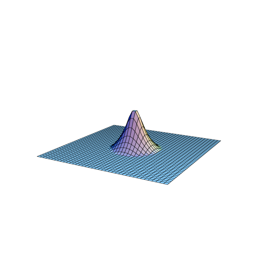
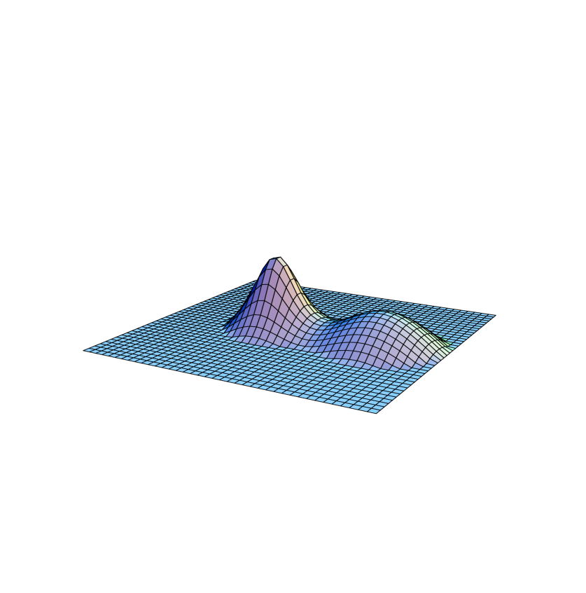
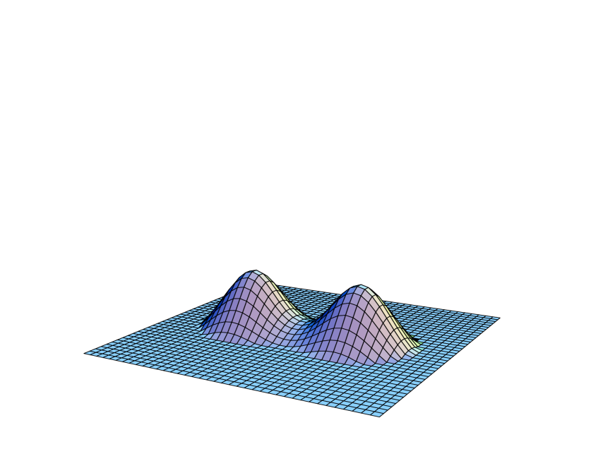
Figure 1: Profiles for calorons at $\omega=0$, 0.125, 0.25 (from top to bottom) with $\rho=1$. The axis connecting the lumps, separated by a distance $\pi$ (for $\omega\neq 0$), corresponds to the direction of $\hat{\omega}$. The other direction indicates the distance to this axis, making use of the axial symmetry of the solutions. Vertically is plotted the action density, at the time of its maximal value, on equal logarithmic scales for the three profiles. The profiles were cut off at an action density below $1/e$. The mass ratio of the two lumps is approximately $\omega/\bar{\omega}$, i.e. zero (no second lump), a third and one (equal masses), for the respective values of $\omega$.

and in a sense the solution can be seen as being built from a suitable combination of two dyons (BPS monopoles) of opposite charge, best understood in terms of an old construction by Taubes involving non-contractible loops in Yang-Mills configuration space [17]. The parameter $\rho$ is related to the scale of the instanton solution, and the two constituent BPS monopoles are separated by a distance $\pi\rho^{2}$. Their mass ratio approaches $\omega/\bar{\omega}$ for large $\rho$, when the solution becomes static (in a suitable gauge). Some of these features are illustrated in figure 1. For $\omega=0\mbox{\,mod\,}{\scriptstyle{{1\over 2}}}$, $P_{\infty}=\pm 1$, the gauge symmetry is no longer broken to the $U(1)$ subgroup generated by $\hat{\omega}\cdot\vec{\tau}$. In this case one of the two radii will drop out of the problem and the solution is spherically symmetric. The relation to the BPS monopole for large $\rho$ at $\omega=0$ can already be found in ref. [18]. The constituent monopole description is also the basis for the results in ref. [14], and seems to be the natural framework for discussing the situation for arbitrary gauge groups, going back to the work of Nahm [6].

For the case $P_{\infty}=\pm 1$ one finds $\chi=\chi^{*}=1-\phi^{-1}$ and $A_{\mu}={\scriptstyle{{1\over 2}}}i\tau_{j}\bar{\eta}^{j}_{\mu\nu}\partial_{\nu}\log\phi$, which is in the form of the celebrated ’t Hooft ansatz [19], and for which $\phi^{-1}\partial_{\mu}^{2}\phi=0$. For non-trivial values of $\omega$ such a simple characterisation is not readily available. Nevertheless, the expression of $\mbox{\,tr}F_{\mu\nu}^{2}(x)=-\partial_{\mu}^{2}\partial_{\nu}^{2}\log\phi$, derived for the ’t Hooft ansatz [19], has a remarkable generalisation to the case of non-trivial $\omega$,

$$\mbox{\,tr}F_{\mu\nu}^{2}(x)=-\partial_{\mu}^{2}\partial_{\nu}^{2}\log\psi.$$ (7)

This equation was used for constructing figure 1. We have also computed numerically the curvature directly from eq. (4), checking the self-duality and verifying eq. (7).

Finally we note that $\omega$ should not be considered as part of the moduli. For each $\vec{\omega}$ one has a different set of solutions. This is particularly clear when we transform to the periodic gauge, for which $A_{0}=2\pi i\vec{\omega}\cdot\vec{\tau}$ at $|\vec{x}|\rightarrow\infty$. For each choice of $\vec{\omega}$ we have an eight dimensional moduli space with as parameters the position of the caloron, which can be obtained by translating our solution in space and time, the scale $\rho$ and a combined rotation and gauge transformation (keeping $P_{\infty}$ fixed).

3 The construction

Rather than presenting the Nahm transformation [5, 6], we make a shortcut by describing the ADHM construction [10], and showing how from an infinite periodic array of instantons (no longer oriented parallel in group space [15]) we can obtain the caloron. Input from the Nahm transformation comes at the point where we interpret the quaternionic valued matrices and vectors that appear in the ADHM construction (collectively known as ADHM data) as the Fourier coefficients with respect to $z$, appearing in the Nahm transformation. The main advantage of this approach is that already much is known about the calculus of multi-instantons in the ADHM formalism [11], in particular also for computing the metric on the moduli space [20]. The ADHM data are obtained after applying the Nahm transformation. Applying this transformation for the second time yields the construction of the self-dual field in terms of the ADHM parameters [13].

Specifically, for charge $k$ $SU(2)$ instantons the ADHM data are given by a quaternionic valued vector $\lambda=(\lambda_{1},\lambda_{2},\cdots,\lambda_{k})$ and a symmetric quaternionic valued $k\times k$ matrix $B$. We parametrise the quaternions as linear combinations of the unit quaternions, $\sigma_{0}=1_{2}$ and $\sigma_{j}=i\tau_{j}$. The vector $\lambda$ is directly related to the asymptotic behaviour of the zero-modes for the Weyl operator, which gives rise to the boundary terms mentioned in the introduction (see ref. [6, 11, 13] for details). This will be seen to be responsible for the announced delta function singularities in the case of calorons. The matrix $B$ is related directly to the connection for the Nahm bundle. In order for the ADHM data to describe a self-dual connection, they have to satisfy a quadratic relation which states that $B^{\dagger}B+\lambda^{\dagger}\lambda$ is a non-singular symmetric $k\times k$ matrix whose entries are real (i.e. proportional to $\sigma_{0}$). Alternatively one may state that $B^{\dagger}B+\lambda^{\dagger}\lambda$ has to commute with the quaternions.

We replace $B$ by $B-x$, with $x=x_{\mu}\sigma_{\mu}$ (a $k\times k$ unit matrix is implicit in our notation). The quadratic ADHM relation obviously remains valid. We note that $x$ corresponds precisely to adding the flat $U(1)$ connection to the Nahm connection when applying the Nahm transformation for the second time. The self-dual gauge field is now given by [10]

$$A_{\mu}(x)=\frac{u^{\dagger}(x)(\partial_{\mu}u(x))-(\partial_{\mu}u^{\dagger}(x))u(x)}{2(1+u^{\dagger}(x)u(x))},\quad u^{\dagger}(x)=\lambda(B-x)^{-1}.$$ (8)

There remains a redundancy which can be related to the gauge invariance for the Nahm bundle,

$$\lambda\rightarrow q\lambda T,\quad B\rightarrow T^{-1}BT,\quad A_{\mu}(x)\rightarrow qA_{\mu}(x)\bar{q},$$ (9)

where $q$ is a unit quaternion ($q\bar{q}=|q|^{2}=1$), i.e. a constant gauge transformation (we use $\bar{x}$ to denote the conjugate quaternion $x^{\dagger}$, note $\bar{q}=q^{-1}$), and $T$ is an orthogonal $k\times k$ matrix with real entries. This can be used to count the number of moduli of a charge $k$ instanton, being $8k-3$. Including the $q$ as moduli gives $8k$ parameters, forming a hyperKähler manifold [12, 21].

The boundary condition $A_{\mu}(x+1)=\exp(2\pi i\vec{\omega}\cdot\vec{\tau})A_{\mu}(x)\exp(-2\pi i\vec{\omega}\cdot\vec{\tau})$ is compatible with the algebraic nature of the ADHM construction, and can be implemented by

$$\lambda_{n}=\exp(2\pi in\vec{\omega}\cdot\vec{\tau})\zeta,\quad B_{m,n}=B_{m-1,n-1}+\delta_{m,n},$$ (10)

with $\zeta$ an arbitrary quaternion, such that

$$u_{m+1}(x+1)=u_{m}(x)\exp(-2\pi i\vec{\omega}\cdot\vec{\tau}).$$ (11)

We note that this means $k=\infty$. Indeed, $A_{\mu}(x)$ viewed as a solution on $R^{4}$ with unit topological charge per period has an infinite total topological charge. For trivial holonomy ($\omega\equiv|\vec{\omega}|=0\mbox{\,mod\,}{\scriptstyle{{1\over 2}}}$) it is seen that the quadratic constraint on the ADHM data is solved by choosing $B_{m,n}=(m+\xi)\delta_{m,n}$, with $\xi$ an arbitrary quaternion, which describes the position of the caloron. The caloron size is given by $\rho=|\zeta|$ and $\zeta/\rho$ represents a constant gauge transformation.

The major obstacle for non-trivial holonomy was satisfying the non-linear constraint. This can be solved most easily by introducing a Fourier transformation [22]. Let us first give the solution in the matrix representation

$$B_{m,n}=(m+\xi)\delta_{m,n}+\hat{A}_{m,n},\quad\hat{A}_{m,n}=i\bar{\zeta}\hat{\omega}\cdot\tau\zeta\frac{\sin(2\pi\omega(m-n))}{m-n}(1-\delta_{m,n}).$$ (12)

It has the right number of parameters, 8 in total, where $q\equiv\zeta/\rho$ is split in a $U(1)$ part commuting with $P_{\infty}$, describing the residual $U(1)$ gauge invariance, and a part $SU(2)/U(1)$ describing a rotation of the vector $\vec{\omega}$, compensated by a gauge transformation to ensure that $P_{\infty}$, or equivalently the periodicity condition, is unaltered.

It is advantageous to first give some general results, valid for arbitrary instantons, which seem to be new and give a more efficient way of representing $A_{\mu}(x)$. The derivation is straightforward and will presented elsewhere. It is well known that in this problem two Green’s functions appear [6, 11]. One is associated to the quadratic ADHM relation

$$f_{x}=(\Delta^{\dagger}(x)\Delta(x))^{-1},\quad\Delta^{\dagger}(x)=(\lambda^{\dagger},(B-x)^{\dagger}),\quad\Delta^{\dagger}(x)\Delta(x)=(B-x)^{\dagger}(B-x)+\lambda^{\dagger}\lambda.$$ (13)

$\Delta^{\dagger}(x)$ is a $k\times(k+1)$ dimensional quaternionic matrix. Self-duality implies that $f_{x}$ commutes with the quaternions. The other Green’s function is given by

$$G_{x}=((B-x)^{\dagger}(B-x))^{-1}.$$ (14)

From the definition of $u(x)$ it follows that

$$\phi\equiv 1+\lambda G_{x}\lambda^{\dagger}=1+u^{\dagger}(x)u(x).$$ (15)

One finds the following compact result

$$A_{\mu}(x)=-{\scriptstyle{{1\over 2}}}\phi\partial_{\nu}\left(\phi^{-1}(\lambda\bar{\eta}_{\nu\mu}G_{x}\lambda^{\dagger})\right),$$ (16)

where $\bar{\eta}_{\mu\nu}\equiv\sigma_{i}\bar{\eta}^{i}_{\mu\nu}$ (the ’t Hooft tensors [16] may be defined through $\bar{\eta}_{\mu\nu}={\scriptstyle{{1\over 2}}}(\bar{\sigma}_{\mu}\sigma_{\nu}-\bar{\sigma}_{\nu}\sigma_{\mu})$ and $\eta_{\mu\nu}={\scriptstyle{{1\over 2}}}(\sigma_{\mu}\bar{\sigma}_{\nu}-\sigma_{\nu}\bar{\sigma}_{\mu})$).

By choosing $B$ diagonal and the entries of $B$ and $\lambda$ real, this result immediately leads to the subclass of solutions that are expressed in terms of the ’t Hooft ansatz [19]. The quadratic ADHM condition is obviously satisfied, and $A_{\mu}(x)={\scriptstyle{{1\over 2}}}\bar{\eta}_{\mu\nu}\partial_{\nu}\log\phi$.

We note that the Green’s functions $f_{x}$ and $G_{x}$ are intimately related. In particular

$$G_{x}\lambda^{\dagger}=\phi f_{x}\lambda^{\dagger},$$ (17)

which implies that

$$\phi=(1-\lambda f_{x}\lambda^{\dagger})^{-1},\quad A_{\mu}(x)=-{\scriptstyle{{1\over 2}}}\phi\partial_{\nu}\left(\lambda\bar{\eta}_{\nu\mu}f_{x}\lambda^{\dagger}\right).$$ (18)

As a consequence we will only need to know $f_{x}$. This Green’s function is simpler to determine than $G_{x}$, since $f_{x}$ is a proportional to $\sigma_{0}$. A standard computation, that lies at the heart of showing that the curvature obtained after applying the Nahm transformation is self-dual [6, 11, 8] (for which it is crucial that $f_{x}$ commutes with the quaternions), yields

$$F_{\mu\nu}=2\phi^{-1}u^{\dagger}\eta_{\mu\nu}f_{x}u.$$ (19)

We have now reduced the explicit computation of instanton solutions to the computation of $f_{x}$. Incidentally, it can be verified that all infinite sums involved in expressions that appear for the calorons are convergent. Eq. (19) demonstrates that it gives a self-dual solution. We now discuss the Fourier transformation, in terms of which one solves for the quadratic ADHM constraint and for the Green’s function $f_{x}$. One defines

$$\hat{\lambda}(z)=\sum_{m}\exp(2\pi imz)\lambda_{m}=(P_{+}\delta(z-\omega)+P_{-}\delta(z+\omega))\zeta,$$

$$\delta(z^{\prime}-z)\hat{D}(z)=\sum_{m,n}\exp\left(2\pi i(mz^{\prime}-nz)\right)B_{m,n},$$ (20)

where $P_{\pm}={\scriptstyle{{1\over 2}}}(1\pm\hat{\omega}\cdot\vec{\tau})$. Parametrising $B_{m,n}$ as before in terms of $\xi$ and $\hat{A}_{m,n}$, with $\delta(z^{\prime}-z)\hat{A}(z)=\sum_{m,n}\exp(2\pi i(mz^{\prime}-nz))\hat{A}_{m,n}$, we find

$$\hat{D}(z)=\frac{1}{2\pi i}\frac{d}{dz}+\xi+\hat{A}(z).$$ (21)

Thus, $B$ has been turned into a differential operator, precisely the Weyl operator appearing in the Nahm transformation, with $\hat{A}(z)\equiv\hat{A}_{\mu}(z)\sigma_{\mu}$ the connection for the Nahm bundle [13] (up to factors $2\pi i$, to match with the conventions of the ADHM construction). The Nahm transformation would require $\hat{D}^{\dagger}\hat{D}$ to commute with the quaternions, which is equivalent to saying that the curvature of the Nahm connection is self-dual. Due to the boundary terms discussed in the introduction, this self-duality is violated at a finite number of points [13] and the presence of $\lambda^{\dagger}\lambda$ in the quadratic ADHM relation is precisely so as to correct for the violations of self-duality, in accordance with the expectations expressed in the introduction. After Fourier transformation this quadratic relation reads, with a slight abuse of notation,

$$(\Delta^{\dagger}(x)\Delta(x))(z)\equiv(\hat{D}(z)-x)^{\dagger}(\hat{D}(z)-x)+\hat{\Lambda}(z),$$ (22)

where

$$\delta(z^{\prime}-z)\hat{\Lambda}(z)=\hat{\lambda}^{\dagger}(z^{\prime})\hat{\lambda}(z),\quad\hat{\Lambda}(z)=\bar{\zeta}\left(P_{+}\delta(z-\omega)+P_{-}\delta(z+\omega)\right)\zeta.$$ (23)

The condition that $\Delta^{\dagger}(x)\Delta(x)$ has to commute with the quaternions is now seen to lead to the equation

$$d\hat{A}(z)/dz=\pi\bar{\zeta}\hat{\omega}\cdot\vec{\sigma}\zeta(\delta(z+\omega)-\delta(z-\omega)),$$ (24)

which is solved by (eliminating an arbitrary additive constant that can be absorbed in $\xi$ by imposing $\int^{1}_{0}dz\hat{A}(z)=0$),

$$\hat{A}(z)=\bar{\zeta}\hat{\omega}\cdot\vec{\sigma}\zeta\hat{A}^{(0)}(z),\quad\hat{A}^{(0)}(z)=\pi(1-2\omega-\chi_{\omega}(z)),$$ (25)

where $\chi_{\omega}(z)=1$ for $\omega<z<1-\omega$ (requiring $\omega\in[0,{\scriptstyle{{1\over 2}}}]$) and 0 elsewhere. Fourier transformation of $\hat{A}(z)$ yields the result in eq. (12).

As $x$ and $\xi$ always occur in the combination $x-\xi$, we absorb $\xi$ by a translation in $x$. The computation of $f_{x}$ now reduces to a one-dimensional quantum mechanical problem on the circle,

$$\left\{\left(\frac{1}{2\pi i}\frac{d}{dz}-x_{0}\right)^{2}\!+\!r^{2}\chi_{\omega}(z)\!+\!s^{2}(1\!-\!\chi_{\omega}(z))\!+\!{\scriptstyle{{1\over 2}}}\rho^{2}(\delta(z\!+\!\omega)\!+\!\delta(z\!-\!\omega))\right\}f_{x}(z,z^{\prime})=\delta(z-z^{\prime}),$$ (26)

where the radii $r$ and $s$ were given in eq. (6) (note that here $\vec{a}\!\cdot\!\vec{\sigma}=\bar{\zeta}\hat{\omega}\!\cdot\!\vec{\sigma}\zeta$). We will present the explicit analytic solution for $f_{x}(z,z^{\prime})$ elsewhere, but it should be noted that, due to the particular form of $\hat{\lambda}(z)$, only $f_{x}(\omega,\omega)=f_{x}(-\omega,-\omega)$ and $f_{x}(\omega,-\omega)=f_{x}(-\omega,\omega)^{*}$, respectively real and complex functions of $x_{\mu}$, will occur in the evaluation of $A_{\mu}(x)$ (see eq. (18)). To obtain eq. (4) from eq. (18), one moves $\bar{\eta}_{\mu\nu}$ through $\hat{\lambda}(z)$, which for non-trivial $\omega$ do not commute.

We close this section by quoting a useful and remarkable result [11, 20],

$$\mbox{\,tr}F_{\mu\nu}^{2}(x)=-\partial_{\mu}^{2}\partial_{\nu}^{2}\log\det(f_{x}),$$ (27)

which leads to the result given in eq. (7). Although for the caloron $\log\det(f_{x})$ is divergent, $\partial_{\mu}\log\det(f_{x})$ is well defined.

4 The geometry of moduli space

The moduli space of the self-dual solutions is given by the ADHM data, or equivalently by the Nahm connections. The latter are self-dual connections on the dual space and the Nahm transformation provides precisely a T-duality [9]. It has been well established that this transformation preserves the metric and hyperKähler structure of the moduli spaces [8, 12]. By computing this metric on the moduli space we can determine its geometry. We use results due to Osborn [20], which can be readily transposed to the case of the calorons and become particularly elegant after the Fourier transformation.

Since we have a closed expression for $A_{\mu}(x)$ in terms of the ADHM parameters, we can compute the variations $\delta A_{\mu}(x)$ with respect to the moduli in terms of variations of the ADHM data, summarised in terms of $\delta\Delta(x)$. The metric is obtained by computing $||\delta A||^{2}=-\int d_{4}x\mbox{\,tr}(P\delta A_{\mu}(x))^{2}$, where $P$ is the projection on the transverse gauge fields, achieved by applying an infinitesimal gauge transformation such that $\delta A^{\prime}_{\mu}(x)$ satisfies the background gauge condition $D_{\mu}\delta A^{\prime}_{\mu}(x)=0$. It can be shown that [20]

$$D_{\mu}\delta A_{\mu}(x)=\phi^{-1}u^{\dagger}f_{x}\sigma_{\mu}\left((\delta\Delta^{\dagger})\Delta-\Delta^{\dagger}(\delta\Delta)\right)\bar{\sigma}_{\mu}f_{x}u,$$ (28)

which vanishes if and only if ${\scriptstyle{{1\over 2}}}\mbox{\,tr}\left((\delta\Delta^{\dagger})\Delta-\Delta^{\dagger}(\delta\Delta)\right)=0$. This condition is precisely the background gauge condition for the Nahm connection (for $T^{4}$ this is an exact statement [8], whereas in general $\lambda$ provides the corrections due the asymptotic behaviour of the chiral zero-modes of the Weyl operator). In particular this implies that the background gauge condition is preserved under the Nahm, or T-duality, transformation. Projection to a transverse variation of the connection can therefore be achieved by applying an infinitesimal gauge transformation to the ADHM data as given in eq. (9) ($q=1$). Under such an infinitesimal gauge transformation, $T=\exp(\delta X)=1+\delta X+\cdots$,

$$\delta_{X}\lambda=\lambda\delta X,\quad\delta_{X}B=[B,\delta X],\quad\delta X^{\dagger}=-\delta X.$$ (29)

Replacing $\delta\Delta$ by $C_{X}\equiv\delta\Delta+\delta_{X}\Delta$, the background gauge condition gives an equation for $\delta X$ in terms of $\delta\Delta$,

$${\scriptstyle{{1\over 2}}}\mbox{\,tr}\left(B^{\dagger}[B,\delta X]-[B^{\dagger},\delta X]B+2\delta X\Lambda+\Delta^{\dagger}\delta\Delta-\delta\Delta^{\dagger}\Delta\right)=0.$$ (30)

For the caloron, with $\delta X$ preserving the periodicity (11), the transformation of $\delta\Delta$ to a transverse variation can now be reformulated after Fourier transformation as

$$-\frac{1}{4\pi^{2}}\frac{d^{2}\delta\hat{X}(z)}{dz^{2}}+|\zeta|^{2}(\delta(z-\omega)+\delta(z+\omega))\delta\hat{X}(z)=\frac{i}{4}\mbox{\,tr}\left((\delta\zeta\bar{\zeta}-\zeta\delta\bar{\zeta})\hat{\omega}\cdot\vec{\sigma}\right)(\delta(z-\omega)-\delta(z+\omega)),$$ (31)

where $\delta(z^{\prime}-z)\delta\hat{X}(z)=\sum_{m,n}\exp(2\pi i(mz^{\prime}-nz))\delta X_{m,n}$. Solving for $\delta\hat{X}(z)$ gives

$$\delta\hat{X}(z)=-\pi i\frac{\mbox{\,tr}\left((\delta\zeta\bar{\zeta}-\zeta\delta\bar{\zeta})\hat{\omega}\cdot\vec{\sigma}\right)}{1+4\pi^{2}\omega(1-2\omega)|\zeta|^{2}}\int_{0}^{z}dz^{\prime}\hat{A}^{(0)}(z^{\prime}),$$ (32)

which is a zig-zag function (periodic and odd in $z$), with discontinuous derivatives at $z=\pm\omega$.

The following miraculous formula due to Osborn [20] allows us to compute $||\delta A||^{2}$,

$$\mbox{\,tr}(P\delta A_{\mu}(x))^{2}={\scriptstyle{{1\over 2}}}\partial_{\mu}^{2}\mbox{\,tr}\mbox{\,Tr}\left(C_{X}^{\dagger}(2-\Delta(x)f_{x}\Delta^{\dagger}(x))C_{X}f_{x}\right).$$ (33)

Since the right-hand side of this equation is smooth and a total derivative, the integration over space and time is completely determined by the behaviour for $r=|\vec{x}|\rightarrow\infty$. In this limit we may replace $f_{x}(z,z^{\prime})$ by $\pi r^{-1}\exp\left(-2\pi r|z-z^{\prime}|+2\pi ix_{0}(z-z^{\prime})\right)$ (near $z=z^{\prime}$, properly extended as a function on $S^{1}\times S^{1}$). From this we find

$$||\delta A||^{2}=2\pi^{2}\mbox{\,tr}\int^{1}_{0}dz\left\{d\hat{B}^{\dagger}(z)d\hat{B}(z)+2d\hat{\lambda}^{\dagger}(z)\int_{0}^{1}dz^{\prime}d\hat{\lambda}(z^{\prime})\right\},$$ (34)

where

$$d\hat{\lambda}(z) \equiv P_{+}\delta(z-\omega)(\delta\zeta+\zeta\delta\hat{X}(\omega))+P_{-}\delta(z+\omega)(\delta\zeta-\zeta\delta\hat{X}(\omega)),$$

$$d\hat{B}(z) \equiv \delta\xi+\delta\hat{A}(z)+\frac{1}{2\pi i}\frac{d\delta\hat{X}(z)}{dz}.$$ (35)

For the metric one finds the explicit result

$$||\delta A||^{2}=4\pi^{2}|\delta\xi|^{2}+8\pi^{2}(1+R^{2})|\delta\zeta|^{2}-2\pi^{2}R^{2}|\zeta|^{2}(1+\frac{1}{1+R^{2}})(\hat{\omega}\cdot\delta\vec{\sigma})^{2},$$ (36)

where ($\zeta\equiv y_{\mu}\sigma_{\mu}$)

$$R^{2}=\pi^{2}|\zeta|^{2}/M^{2},\quad M^{-2}=8\omega(1-2\omega),\quad{\scriptstyle{{1\over 2}}}\delta\sigma_{j}=\eta^{j}_{\mu\nu}|\zeta|^{-2}y_{\mu}dy_{\nu}.$$ (37)

One readily recognises, putting $\delta\xi=0$, the Taub-NUT metric [23] with mass $M$. For $\hat{\omega}$ in the third direction this metric is given by [24]

$$ds^{2}=(1+\frac{x^{2}}{16M^{2}})\left(dx^{2}+{\scriptstyle{{1\over 4}}}x^{2}(d\sigma_{1}^{2}+d\sigma_{2}^{2})\right)+{\scriptstyle{{1\over 4}}}x^{2}d\sigma_{3}^{2}/(1+\frac{x^{2}}{16M^{2}}),$$ (38)

where we identify $x^{2}=8\pi^{2}\rho^{2}$. We note that the Taub-NUT space is a self-dual Einstein manifold [25] and that it has a hyperKähler structure [26], inherited from the hyperKähler structure of $R^{3}\times S^{1}$.

5 Conclusions

We have found the explicit charge one $SU(2)$ caloron solutions with the Polyakov loop at spatial infinity non-trivial. Previously only solutions for which the latter was trivial were known [1]. Those were argued to dominate in the instanton contribution to the finite temperature partition function [15], a question that can now more directly be addressed and is perhaps of physical significance.

We have shown that the moduli space of these solutions forms a Taub-NUT space, providing an exact classical T-duality between H-monopoles and Kaluza-Klein monopoles [4]. Indeed it is well-known that the Taub-NUT metric describes (the spatial part of) the Kaluza-Klein monopole [27] with compactification radius $4M$. Most importantly we have related the holonomy to the compactification radii involved in the dual descriptions.

References

• [1] B.J. Harrington and H.K. Shepard, Phys. Rev. D17 (1978) 2122; D18 (1978) 2990.
• [2] J.P. Gauntlett, J.A. Harvey and J. Liu, Nucl. Phys. B409 (1993) 363; J.P. Gauntlett and J.A. Harvey, S-Duality and the Spectrum of Magnetic Monopoles in Heterotic String Theory, hep-th/9407111.
• [3] R. Rohm and E. Witten, Ann. Phys. (N.Y.) 170 (1986) 454.
• [4] R. Gregory, J.A. Harvey and G. Moore, Unwinding Strings and T-duality of Kaluza-Klein and H-monopoles, hep-th/9708086.
• [5] W. Nahm, Phys. Lett. 90B (1980) 413; The construction of all self-dual multimonopoles by the ADHM method, in ”Monopoles in quantum field theory”, eds. N. Craigie, e.a. (World Scientific, Singapore, 1982).
• [6] W. Nahm, Self-dual monopoles and calorons, in: Lect. Notes in Physics. 201, eds. G. Denardo, e.a. (1984) p. 189.
• [7] S. Mukai, Invent. Math. 7 (1984) 101.
• [8] P.J. Braam and P. van Baal, Commun. Math. Phys. 122 (1989) 267.
• [9] M.R. Douglas and G. Moore, D-branes, quivers, and ALE instantons, hep-th/9603167; D.-E. Diaconescu, Nucl. Phys. B503 (1997) 220 (hep-th/9608163); J.-S. Park, Nucl. Phys. B493 (1997) 198 (hep-th/9612096); F. Hacquebord and H. Verlinde, Nucl. Phys. B508 (1997) 609 (hep-th/9707179).
• [10] M.F. Atiyah, N.J. Hitchin, V.G. Drinfeld and Yu.I. Manin, Phys. Lett. 65A (1978) 185; M.F. Atiyah, Geometry of Yang-Mills fields, Fermi lectures, (Scuola Normale Superiore, Pisa, 1979).
• [11] E. Corrigan and P. Goddard, Ann. Phys. (N.Y.) 154 (1984) 253.
• [12] S.K. Donaldson and P.B. Kronheimer, The Geometry of Four-Manifolds, (Clarendon Press, Oxford, 1990).
• [13] P. van Baal, Nucl. Phys. B(Proc. Suppl.)49 (1996) 238 (hep-th/9512223).
• [14] K. Lee, Instantons and Magnetic Monopoles on $R^{3}\times S^{1}$ with Arbitrary Simple Gauge Groups, hep-th/9802012.
• [15] D.J. Gross, R.D. Pisarski and L.G. Yaffe, Rev. Mod. Phys. 53 (1983) 43.
• [16] G. ’t Hooft, Phys. Rev. D14 (1976) 3432.
• [17] C. Taubes, Commun. Math. Phys. 86 (1982) 257, 299; in: Progress in gauge field theory, eds. G. ’t Hooft et al, (Plenum Press, New York, 1984) p. 563.
• [18] P. Rossi, Nucl. Phys. B149 (1979) 170.
• [19] G. ’t Hooft, as quoted in R. Jackiw, C. Nohl and C. Rebbi, Phys. Rev. D15 (1977) 1642; R. Rajaraman, Solitons and Instantons, (North-Holland, Amsterdam, 1982).
• [20] H. Osborn, Ann. Phys. (N.Y.) 135 (1981) 373.
• [21] S.K. Donaldson, Commun. Math. Phys. 96 (1984) 387.
• [22] T.C. Kraan, Nahm’s transformation and instantons on $R^{3}\times S^{1}$, poster presented at the 2nd DRSTP symposium, Dalfsen, The Netherlands, 5-6 June, 1997 (unpublished).
• [23] E.T. Newman, T. Unti and L. Tamburino, J. Math. Phys. 4 (1963) 915.
• [24] S. Hawking, in: General Relativity, an Einstein centenary survey, ed. S. Hawking and W. Israel, (Cambridge Univ. Press, 1979) p. 774.
• [25] G. Gibbons and C. Pope, Commun. Math. Phys. 66 (1979) 267.
• [26] N.J. Hitchin, A. Karlhede, U. LindstrΓΆm and M. Roček, Commun. Math. Phys. 108 (1987) 535; M.F. Atiyah and N.J. Hitchin, The Geometry and Dynamics of Magnetic Monopoles, (Princeton Univ. Press, 1988) ch. 9.
• [27] R. Sorkin, Phys. Rev. Lett. 51 (1983) 87; D. Gross and M.Perry, Nucl. Phys. B226 (1983) 29.
Refer to caption
Refer to caption
Refer to caption