Zero-Mode Problem on the Light Front

Abstract

A series of lectures are given to discuss the zero-mode problem on the light-front (LF) quantization with special emphasis on the peculiar realization of the trivial vacuum, the spontaneous symmetry breaking (SSB) and the Lorentz invariance. We first identify the zero-mode problem on the LF. We then discuss Discrete Light-Cone Quantization (DLCQ) which was first introduced by Maskawa and Yamawaki (MY) to solve the zero-mode problem and later advocated by Pauli and Brodsky in a different context. Following MY, we present canonical formalism of DLCQ and the zero-mode constraint through which the zero mode can actually be solved away in terms of other modes, thus establishing the trivial vacuum. Due to this trivial vacuum, existence of the massless Nambu-Goldstone (NG) boson coupled to the current is guaranteed by the non-conserved charge such that $Q|0\rangle=0$ and $\dot{Q}\neq 0$ but not by the NG theorem which in the equal-time quantization ensures existence of the massless NG boson coupled to the current with the charge $Q|0\rangle\neq 0$ and $\dot{Q}=0$. The SSB (NG phase) in DLCQ can be realized on the trivial vacuum only when an explicit symmetry-breaking mass of the NG boson $m_{\pi}$ is introduced so that the NG-boson zero mode integrated over the LF exhibits singular behavior $\sim 1/m_{\pi}^{2}$ in such a way that $\dot{Q}\neq 0$ in the symmetric limit $m_{\pi}\rightarrow 0$. We also demonstrate this realization more explicitly in a concrete model, the linear sigma model, where the role of zero-mode constraint is clarified. We further point out, in disagreement with Wilson et al., that for SSB in the continuum LF theory, the trivial vacuum collapses due to the special nature of the zero mode which is no longer the problem of a single mode $P^{+}\equiv 0$ but of the accumulating point $P^{+}\rightarrow 0$, in sharp contrast to DLCQ. Finally, we discuss the no-go theorem of Nakanishi and Yamawaki, which forbids exact LF restriction of the field theory that satisfies the Wightman axioms. The well-defined LF theory exists only at the sacrifice of the Lorentz invariance. Thus DLCQ as well as any other regularization on the exact LF has no Lorentz-invariant limit as the theory itself, although we can argue, based on an explicit solution of the dynamics (i.e., perturbation), that the Lorentz-invariant limit can be realized on the c-number quantity like S matrix which has no reference to the fixed LF.

0 Introduction

Much attention has recently been paid to the light-front (LF) quantization[1] as a promising approach to solve the non-perturbative dynamics [2, 3, 4]. The most important aspect of the LF quantization is that the physical LF vacuum is simple, or even trivial [5]. However, such a trivial vacuum, which is vital to the whole LF approach, can be realized only if we can remove the so-called zero mode out of the physical Fock space (“zero mode problem”[6]).

Actually, the Discrete Light-Cone Quantization (DLCQ) was first introduced by Maskawa and Yamawaki (MY)[6] in 1976 to resolve the zero mode problem and was advocated by Pauli and Brodsky[8] in 1985 in a different context. The zero mode in DLCQ is clearly isolated from other modes and hence can be treated in a well-defined manner without ambiguity, in sharp contrast to the continuum theory where the zero mode is the accumulating point and hard to be controlled in isolation [9, 10]. In DLCQ, MY[6] in fact discovered a constraint equation for the zero mode (“zero-mode constraint”) through which the zero mode becomes dependent on other modes and then they observed that the zero mode can be removed from the physical Fock space by solving the zero-mode constraint, thus establishing the trivial LF vacuum in DLCQ.

Such a trivial vacuum, on the other hand, might confront the usual picture of complicated non-perturbative vacuum structure in the equal-time quantization corresponding to confinement, spontaneous symmetry breaking (SSB), etc.. Since the vacuum is proved trivial in DLCQ [6], the only possibility to realize such phenomena would be through the complicated structure of the operator and only such an operator would be the zero mode. In fact the zero-mode constraint implies that the zero mode carries essential information on the complicated dynamics. One might thus expect that explicit solution of the zero-mode constraint in DLCQ would give rise to the SSB while preserving the trivial LF vacuum. Actually, several authors have argued in (1+1) dimensional models that the solution to the zero-mode constraint might induce spontaneous breaking of the discrete symmetries [11, 12, 13]. However, the most outstanding feature of the SSB is the existence of the Nambu-Goldstone (NG) boson for the continuous symmetry breaking in (3+1) dimensions.

In recent works done in collaboration with Yoonbai Kim and Sho Tsujimaru [14, 10], we in fact found, within the canonical formalism of DLCQ[6], how the SSB manifests itself on LF in (3+1) dimensions through existence of the NG boson while keeping the vacuum trivial.

In the above works[14, 10] we encountered a striking feature of the zero mode of the NG boson: Naive use of the zero-mode constraint does not lead to the NG phase at all, with the NG boson being totally decoupled ((false) “no-go theorem”). It implies that the above approach[11, 12, 13], as it stands, fails to realize the NG phase. Indeed it is inevitable to introduce an infrared regularization through explicit-breaking mass of the NG boson $m_{\pi}$. The NG phase can only be realized via peculiar behavior of the zero mode of the NG-boson field: The NG-boson zero mode, when integrated over the LF, must have a singular behavior $\sim 1/m_{\pi}^{2}$ in the symmetric limit $m_{\pi}^{2}\rightarrow 0$. This was demonstrated both in a general framework of the LSZ reduction formula and in a concrete field theoretical model, the linear sigma model. The NG phase is in fact realized in such a way that the vacuum is trivial, $Q|0\rangle=0$, while the LF charge $Q$ is not conserved, $\dot{Q}\neq 0$, even in the symmetric limit $m_{\pi}^{2}\rightarrow 0$.

Note that this is not an artifact of DLCQ but is a general feature of NG phase realized on the trivial vacuum of LF: As far as the vacuum is trivial and hence symmetric, the only possibility to realize the non-symmetric physical world is that the Hamiltonian is not symmetric at quantum level (if both vacuum and Hamiltonian were symmetric, then the physical world would also be symmetric). It might look like the usual explicit symmetry breaking but is essentially different in the sense that we do have massless NG boson coupled to the current. The existence of massless NG boson coupled to the current is in fact ensured by the charge $Q|0\rangle=0$ and $\dot{Q}\neq 0$, which is quite opposite to the NG theorem in the equal-time quantization with the charge $Q|0|\rangle\neq 0$ and $\dot{Q}=0$. The above singular behavior of the NG-boson zero mode is thus a manifestation of the same SSB phenomenon as that dictated by the NG theorem of the equal-time quantization, though in a way quite different than the NG theorem.

It is rather remarkable that in the continuum theory the SSB cannot be formulated consistently with the trivial vacuum [10] in sharp contrast to DLCQ. It was demonstrated[10] with careful treatment of the boundary condition (B.C.) that as far as the sign function is used for the standard canonical LF commutator, the LF charge does not annihilate the vacuum in the continuum LF theory in disagreement with Wilson et al.[2]. This in fact reflects the problem of the zero mode in the continuum theory: The problem is not a single mode $P^{+}\equiv 0$ with just measure zero but the accumulating point $P^{+}\rightarrow 0$ which cannot be removed by simply dropping the exact zero mode $P^{+}\equiv 0$ [9].

The zero-mode problem in this sense is more serious in the context of Lorentz invariance. There in fact exists a no-go theorem found by Nakanishi and Yamawaki[9] which forbids the exact LF restriction of the field theory that satisfies the Wightman axioms, due to the zero mode as the accumulating point: In particular, even a free theory does not exist on the exact LF. This implies that in order to make the theory well-defined on the exact LF, we are forced to give up some of the Wightman axioms, most naturally the Lorentz invariance. Indeed, the DLCQ and the ”$\nu$-theory”[9], defined on the exact LF, are such theories: The theory itself (operator, Hilbert space, etc) explicitly violates the Lorentz invariance and never recovers it even in the continuum limit of $L\rightarrow\infty$ ($\nu\rightarrow 0$ limit in the $\nu$-theory). It is actually at the sacrifice of the Lorentz invariance that the trivial vacuum is realized in DLCQ and $\nu$-theory. However, even though the theory itself does not recover the Lorentz invariance in these theories, we still can argue [9, 10], at least in the perturbation theory, that the Lorentz invariance is realized on the c-number quantity like the S matrix which has no reference to the fixed LF, while keeping the vacuum polarization absent. Such a program is based on the explicit solution of the dynamics, like perturbation. Actually, recovering the Lorentz invariance is highly dynamical issue in the LF quantization, the situation being somewhat analogous to the lattice gauge theories. The non-perturbative way to recover the Lorentz invariance remains a big challenge for any LF theory.

In this lecture we shall fully discuss the above result and the zero-mode problem in the general context. The lecture is largely based on the above recent works[14, 10] and also on the very old ones[6, 9] which are most relevant to the zero-mode problem.

In Section 1 we first explain a key feature of the LF quantization, the trivial vacuum and physical Fock space. Then we discuss the subtlety of the zero mode which might jeopardize this nice property (zero-mode problem). In Section 2 we give the canonical formalism of DLCQ through the Dirac’s quantization for the constrained system, with particular emphasis on the zero mode: Detailed derivation of the LF commutator and the zero-mode constraint are given. Discussions are also given to the subtlety of the B.C.’s of DLCQ in the continuum limit. In Section 3 we first discuss in general the peculiarity of the realization of the NG phase on the LF by the charge $Q|0\rangle=0$ and $\dot{Q}\neq 0$. Then in DLCQ we show that if we were in the exact symmetric theory with the NG-boson mass exactly zero from the beginning, the NG phase would never be realized on the LF: The NG boson simply decouples even in the continuum limit of DLCQ ((false) “no-go theorem”). We then show that such an inconsistency in DLCQ is resolved by introducing an explicit-symmetry-breaking mass of the NG boson $m_{\pi}$ in such a way that the NG-boson zero mode integrated over LF has a singular behavior $\sim 1/m_{\pi}^{2}$ in the symmetric limit $m_{\pi}^{2}\rightarrow 0$, in accordance with the above general statement $Q|0\rangle=0$ and $\dot{Q}\neq 0$. In Section 4 we demonstrate such a peculiar realization in a concrete model, the linear sigma model, by solving the zero-mode constraint perturbatively. Section 5 is devoted to discussions on the zero-mode problem in the continuum theory: The LF vacuum cannot be trivial in the NG phase due to the peculiarity of the zero mode in the continuum LF theory. In Section 6 we discuss the problem of Lorentz invariance in view of the no-go theorem which forbids the well-defined LF restriction due to the peculiarity of the zero mode. A way to recover the Lorentz invariance is suggested. Summary and discussions are given in Section 7.

1 Trivial Vacuum and Physical Fock Space

The light-front (LF) quantization is based on the field commutator on the LF which is the hypersurface tangent to the light cone (LF coincides with the light cone only in (1+1) dimensions but not in (3+1) dimensions). It is also called null-plane quantization, lightlike quantization, front form, and light-cone quantization (even though in (3+1) dimensions), etc.. Note that the LF quantization is inherent in the Minkowski space, since the LF, the quantization plane, is no longer meaningful in the Euclidean space.

Throughout this lecture we use a convention of the LF coordinate: $x^{\mu}=(x^{+},\vec{x})=(x^{+},x^{-},x^{\bot})$, where

$$x^{\pm}=x_{\mp}\equiv\frac{1}{\sqrt{2}}(x^{0}\pm x^{3}),$$ (1.1)

with $x^{+}$ being the “time” while $x^{-}$ the “space” coordinate along the LF, and $x^{\bot}=-x_{\bot}\equiv(x^{1},x^{2})$. The respective conjugate momenta $p_{\mu}=(p_{+},p_{-},p_{\bot})=(p^{-},\vec{p})$ are

$$p_{\pm}=p^{\mp}\equiv\frac{1}{\sqrt{2}}(p^{0}\mp p^{3}),$$ (1.2)

with $p^{-}$ being the energy while $p^{+}$ the momentum, and $p_{\bot}=-p^{\bot}\equiv-(p^{1},p^{2})$. The momentum operator $P^{+}$ is a translation operator along $x^{-}$ direction and is free from dynamics (kinematical operator), while the energy operator $P^{-}$, the Hamiltonian, is the evolution operator of time $x^{+}$, which carries a whole information of the dynamics (dynamical operator). Then $P^{+}$ is conserved even in virtual processes, while $P^{-}$ is not.

1.1 $P^{+}>0$ and Trivial Vacuum/Physical Fock Space

Now, the most important feature of the LF quantization follows from the spectral condition (see Fig.1): Both $P^{+}$ and $P^{-}$ as well as $P^{0}$ have positive-definite spetra for the physical states, namely,

$$p^{+},\quad p^{-}>0\quad\Longleftrightarrow\quad p^{0}>0.$$ (1.3)

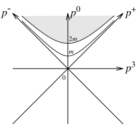
Figure 1: The spectral condition (a single mass system).

This is contrasted to the equal-time case where only the energy operator possesses positive-definite spectrum, $p^{0}>0$, while the momenta can take both positive and negative signs, $\mbox{\boldmath$p$}\equiv(p^{1},p^{2},p^{3})>0\quad{\rm and}<0$. Actually, all the characteristic features of LF quantization simply stem from the fact that $P^{+}$ is a kinematical operator and at the same time has positive-definite spectrum.

First of all it implies that the vacuum is trivial, since we can always specify the eigenvalue of $P^{+}$ without solving the dynamics and the vacuum $|0\rangle$ can be defined kinematically as a state with the lowest eigenvalue of $P^{+}$ without recourse to the $P^{-}$ spectrum; $P^{+}|0\rangle=0$. In view of the spectral condition (1.3) or Fig.1, we may infer that the trivial vacuum is also the true vacuum, namely,

$$P^{+}|0\rangle=0\quad\Longrightarrow\quad P^{-}|0\rangle=0.$$ (1.4)

Upon such a trivial vacuum we can construct the physical Fock space in terms of the interacting Heisenberg field whose Fourier components with $p^{+}>0$ and $p^{+}<0$ are interpreted as the creation and annihilation operators, respectively [5]. This is also viewed as absence of vacuum polarization[15], since all physical states including virtual states must have positive $P^{+}$ and at the same time respect conservation of $P^{+}$ as the kinematical operator (“momentum conservation”) even for the virtual states ($P^{+}>0$) which are to be communicated to the vacuum ($P^{+}=0$) as the initial and final states in the vacuum polarization diagrams.

To be more concrete, let us consider the self-interacting scalar theory in which the interacting Heisenberg field $\phi(x)$ is Fourier-expanded as

$$\phi(x)=\frac{1}{(2\pi)^{3}}\int_{0}^{\infty}\frac{dp^{+}}{2p^{+}}\int_{-\infty}^{\infty}dp^{\bot}\left(a(\vec{p},x^{+})e^{-i\vec{p}\vec{x}}+a^{\dagger}(\vec{p},x^{+})e^{i\vec{p}\vec{x}}\right),$$ (1.5)

where we defined

$$a(\vec{p},x^{+})/2p^{+}\equiv\tilde{\phi}(\vec{p},x^{+}),\quad a^{\dagger}(\vec{p},x^{+})/2p^{+}\equiv\tilde{\phi}(-\vec{p},x^{+})\quad(p^{+}>0)$$ (1.6)

and $\vec{p}\vec{x}=p^{+}x^{-}-p^{\bot}x^{\bot}$, with $\vec{p}\equiv(p^{+},-p^{\bot})$ being just momenta having nothing to do with the dynamics.

Now, the Heisenberg operators $a(x^{+})$ and $a^{\dagger}(x^{+})$, whose $x^{+}$-dependence is not solved, can be interpreted as the creation and annihilation operators, respectively, as follows [5]. Let us assume translation invariance, namely existence of the operator $P^{+}$ such that

$$[\phi(x),P^{+}]=i\partial_{-}\phi(x),$$ (1.7)

then it follows from (1.5):

$$[a(\vec{p},x^{+}),P^{+}]=p^{+}a(\vec{p},x^{+}),\quad[a^{\dagger}(\vec{p},x^{+}),P^{+}]=-p^{+}a^{\dagger}(\vec{p},x^{+}).$$ (1.8)

Thus $a(x^{+})$ and $a^{\dagger}(x^{+})$ as they stand are lowering and raising operators of $P^{+}$ eigenvalue, respectively and the spectral condition $P^{+}>0$ dictates existence of the lowest eigenvalue state $|0\rangle$ ($P^{+}|0\rangle=0$), the vacuum, such that

$$a(\vec{p},x^{+})|0\rangle=0,$$ (1.9)

which would coincide with the true vacuum from the spectral condition as in (1.4). The physical Fock space may be constructed by operating the creation operators $a^{\dagger}$’s on the vacuum:

$$|\vec{p}_{1},\vec{p}_{2},\cdot\cdot\cdot,\vec{p}_{n}\rangle_{x^{+}}=a^{\dagger}(\vec{p}_{1},x^{+})a^{\dagger}(\vec{p}_{2},x^{+})\cdot\cdot\cdot a^{\dagger}(\vec{p}_{n},x^{+})|0\rangle$$ (1.10)

up to normalization. On the other hand, the standard canonical commutator on LF reads (we shall discuss the derivation later):

$$\left[\phi(x),\phi(y)\right]_{x^{+}=y^{+}}=-\frac{i}{4}\epsilon(x^{-}-y^{-})\delta(x^{\bot}-y^{\bot}),$$ (1.11)

where $\epsilon(x^{-})$ is the sign function:

$$\epsilon(x^{-})=\frac{i}{\pi}{\cal P}\int_{-\infty}^{+\infty}\frac{dp^{+}}{p^{+}}e^{-ip^{+}x^{-}} = 1\quad(x^{-}>0)$$ (1.12)

$$= -1\quad(x^{-}<0),$$

with ${\cal P}$ being the principal value. From this and the inverse Fourier transform of (1.5),

$$a(\vec{p},x^{+})=2p^{+}\int d\vec{x}e^{i\vec{p}\vec{x}}\phi(x)=i\int d\vec{x}e^{i\vec{p}\vec{x}}\stackrel{{\scriptstyle\leftrightarrow}}{{\partial}}_{-}\phi(x),$$ (1.13)

(similarly for $a^{\dagger}$), we obtain the commutation relation of $a$ and $a^{\dagger}$ of the conventional form:

$$\left[a(\vec{p},x^{+}),a^{\dagger}(\vec{q},x^{+})\right] = 2p^{+}2q^{+}\int d\vec{x}d\vec{y}e^{i\vec{p}\vec{x}}\left[\phi(x),\phi(y)\right]_{x^{+}=y^{+}}e^{-i\vec{q}\vec{y}}$$ (1.14)

$$= (2\pi)^{3}2p^{+}\delta(\vec{p}-\vec{q}).$$

Note again that the $x^{+}$-dependence of $a(x^{+})$ and $a^{\dagger}(x^{+})$ is not solved (they are Heisenberg fields) and whole procedure was done in a purely kinematical way without recourse to the dynamics (information of $P^{-}$).

Here it is useful to compare the above feature of LF quantization with that of the equal-time quantization. One might think the same type of arguments as those for the relation (1.8) could be done for the Fourier component with respect to momenta $\mbox{\boldmath$P$}\equiv(P^{1},P^{2},P^{3})$ instead of $P^{+}$: $\phi(x)=\int\frac{d^{3}\mbox{\boldmath$p$}}{(2\pi)^{3}2p^{0}}\tilde{\phi}(\mbox{\boldmath$p$},x^{0})e^{-i\mbox{\boldmath$p$}\mbox{\boldmath$x$}}.$ Alas, the spectral condition, $\mbox{\boldmath$P$}\equiv(P^{1},P^{2},P^{3})>0$ and $<0$, which implies no lowest eigenvalue state for these operators in sharp contrast to $P^{+}>0$. It is only $P^{0}$ that has positive-definite spectrum $P^{0}>0$ and a relation analogous to (1.8) follows from

$$[\phi(x),P^{0}]=i\partial_{0}\phi(x),$$ (1.15)

instead of (1.7). However, specifying the definite eigenvalue of $P^{0}$ for the Fourier modes is equivalent to solving the dynamics at operator level, which is in general impossible except for the free theory which is completely solved. As everybody knows, in the free theory we in fact can construct the Fock space based on the explicit solution of the free field equation of motion (Klein-Gordon equation) for the Fourier modes $\tilde{\phi}(\mbox{\boldmath$p$},x^{0})$:

$$\ddot{\tilde{\phi}}(\mbox{\boldmath$p$},x^{0})+\omega^{2}\tilde{\phi}(\mbox{\boldmath$p$},x^{0})=0\qquad(\omega\equiv\sqrt{\mbox{\boldmath$p$}^{2}+m^{2}}>0).$$ (1.16)

This is nothing but the harmonic oscillator and of course has two independent solutions:

$$\tilde{\phi}(\mbox{\boldmath$p$},x^{0}) = \frac{1}{2\omega}a(\mbox{\boldmath$p$})e^{-i\omega t}\quad(p^{0}=\omega),$$ (1.17)

$$= \frac{1}{2\omega}a^{\dagger}(-\mbox{\boldmath$p$})e^{i\omega t}\quad(p^{0}=-\omega).$$

These solutions are in fact lowering and raising operators, respectively, of the eigenvalue of $P^{0}$:

$$[a(\mbox{\boldmath$p$}),P^{0}] = i\dot{a}(\mbox{\boldmath$p$})=-\omega a(\mbox{\boldmath$p$}),$$

$$\left[a^{\dagger}(\mbox{\boldmath$p$}),P^{0}\right] = i\dot{a}^{\dagger}(\mbox{\boldmath$p$})=\omega a^{\dagger}(\mbox{\boldmath$p$}).$$ (1.18)

Then the spectral condition $P^{0}>0$ guarantees the existence of the vacuum $|0\rangle$ as the lowest eigenvalue state ($P^{0}|0\rangle=0$) such that $a(\mbox{\boldmath$p$})|0\rangle=0$ as the explicit solution of the dynamics.

1.2 Advantages of the Light-Front Quantization

Having discussed that the physical Fock space can be constructed upon the trivial vacuum even for the interacting Heisenberg field, we may next discuss possible advantages of LF quantization over the equal-time quantization, particularly to study the bound state problems or the strongly-coupled systems.

1) First of all, the fact that the vacuum is trivial with no vacuum polarization suggests a novel way of understanding the non-perturbative phenomena such as the confinement and the spontaneous chiral symmetry breaking which are due to complicated vacuum structure in the conventional picture of the equal-time quantization. Particularly, the absence of vacuum polarization may naturally explain the success of non-relativistic picture of the constituent quark model.

2) Second, we may introduce the wave function [16] $\psi_{P}(\vec{p}_{1},\vec{p}_{2},\cdot\cdot\cdot,\vec{p}_{n})$ for the relativistic bound states $|P\rangle$ which are to be expanded in terms of the physical Fock space (1.10):

$$|P\rangle=\sum_{n}\int\prod_{i}^{n}\left(\frac{d\vec{p}_{i}}{(2\pi)^{3}2p_{i}^{+}}\right)\psi_{P}(\vec{p}_{1},\vec{p}_{2},\cdot\cdot\cdot,\vec{p}_{n})\delta(\vec{P}-\sum_{n}\vec{p}_{n})|\vec{p}_{1},\vec{p}_{2},\cdot\cdot\cdot,\vec{p}_{n}\rangle.$$ (1.19)

Actually, the creation operators of quarks and gluons in QCD are nothing but the partons; The probability $f_{k}(x)=\int\prod_{i}(d\vec{p}_{i}/(2\pi)^{3}2p_{i}^{+})|\psi_{P}(\vec{p}_{1},\vec{p}_{2},\cdot\cdot\cdot,\vec{p}_{n})|^{2}\delta(x-x_{k})$, with $x_{i}\equiv p^{+}_{i}/P^{+}$, is the parton distribution function. On the other hand, in the equal-time quantization the concept of wave function makes sense only in the nonrelativistic limit where the number of particles is conserved and the vacuum polarization is absent.

3) Third, the triviality of the vacuum suggests that even in the NG phase the LF charges $Q_{\alpha}\equiv\int d\vec{x}J^{+}_{\alpha}(x),Q_{5\alpha}\equiv\int d\vec{x}J^{+}_{5\alpha}(x)$ do annihilate the vacuum:

$$Q_{\alpha}|0\rangle=Q_{5\alpha}|0\rangle=0,$$ (1.20)

where $J^{\mu},J^{5\mu}$ are vector and axial-vector currents, respectively. Namely, the vacuum is singlet under the transformation generated by these charges. This fact was known for long time as Jersák-Stern theorem which was proved when massless particle is absent (i.e., not in the chiral symmetric limit) [17, 6] . Thus the chiral $SU(3)_{L}\times SU(3)_{R}$ algebra of LF charges,

$$\left[Q_{\alpha},Q_{\beta}\right] = if_{\alpha\beta\gamma}Q_{\gamma},$$

$$\left[Q_{\alpha},Q_{5\beta}\right] = if_{\alpha\beta\gamma}Q_{5\gamma},$$

$$\left[Q_{5\alpha},Q_{5\beta}\right] = if_{\alpha\beta\gamma}Q_{\gamma},$$ (1.21)

with $\alpha,\beta,\gamma=1,2,\cdot\cdot\cdot,8$, may be useful to classify the physical states which are constructed out of a chain of field operators acting on the vacuum as (1.10). Since the vacuum is singlet and the field operators have definite transformation property of this algebra, the physical states also have definite transformation property. This is in contrast to the equal-time quantization where the vacuum in NG phase is not singlet and hence the physical states do not have definite transformation property even though the field operators do. Actually the chiral algebra of LF charge is nothing but the algebraization of the celebrated Adler-Weisberger (AW) sum rules [18] in hadron physics [19, 20]. Through analysis of AW sum rules, hadrons are in fact classified into (reducible) representations of the LF chiral algebra, which coincides with the one time fashionable “representation mixing” [21, 22, 19, 23, 20]. We shall fully discuss this point in Section 3.

1.3 Zero-Mode Problem

The above arguments, however, are subject to criticism that the zero mode with $p^{+}=0$ has been simply ignored. Actually, from the spectral condition (see Fig.1) there is no gap between the zero mode $p^{+}=0$ and the non-zero modes $p^{+}>0$ and hence it is rather delicate whether the zero mode can be neglected or not. If there exists a zero-mode state degenerate with the trivial vacuum, then the trivial vacuum may not be the true vacuum:

$$P^{+}|0\rangle=0\not\Rightarrow\ P^{-}|0\rangle=0,$$ (1.22)

in contrast to (1.4).

Historically, it was first argued by Weinberg [15] in the perturbation theory that the “vacuum diagrams” (diagrams with lines created/annihilated from/into the vacuum and with external lines, Fig.2) and the vacuum polarization (vacuum to vacuum diagram without external lines, Fig.3) both vanish in the infinite-momentum frame. The result was then re-examined through the Feynman rule in terms of LF parameterization [24];

$$\int d\mbox{\boldmath$p$}dp^{0}\rightarrow\int d\vec{p}dp^{-},$$ (1.23)

with the propagator

$$\Delta_{F}(x;m^{2}) = \theta(x^{+})\Delta^{(+)}(x;m^{2})-\theta(-x^{+})\Delta^{(-)}(x;m^{2})$$ (1.24)

$$= \frac{1}{(2\pi)^{4}}\int d\vec{p}\int dp^{-}\frac{e^{-ip^{-}x^{+}+i\vec{p}\vec{x}}}{2p^{+}p^{-}-p_{\bot}^{2}-m^{2}+i0},$$

where

$$\Delta^{(\pm)}(x;m^{2})=\pm\int\frac{d\vec{p}dp^{-}}{(2\pi)^{3}}\theta(\pm p^{+})\delta(2p^{+}p^{-}-p_{\bot}^{2}-m^{2})e^{-i(p^{-}x^{+}+\vec{p}\vec{x})}.$$ (1.25)

Here we note that $\pm\theta(\pm x^{+})\Delta^{(\pm)}(x;m^{2})\sim\theta(\pm x^{+})\theta(\pm p^{+})\sim\theta(x^{+}p^{+})$ apart form the factor $\frac{1}{(2\pi)^{3}}\int d^{4}p\delta(p^{2}-m^{2})e^{-ipx}$. Note that $\theta(p^{+}x^{+})$ instead of $\theta(p^{-}x^{+})$, in sharp contrast to $\theta(p^{0}x^{0})$ in the equal-time quantization. Then the particle lines with $x^{+}>0$ carry $p^{+}>0$, while the lines with $x^{+}<0$ which carry $p^{+}<0$ are interpreted as anti-particles with $x^{+}>0,p^{+}>0$. This actually led to vanishing vacuum diagrams with external lines (Fig.2), since $P^{+}$ conservation (momentum conservation) forbids the transition between the vacuum ($p^{+}=0$) and the intermediate states ($p^{+}=\sum_{k}p_{k}^{+}>0$ in $x_{k}^{+}>0$ direction) with each internal line having $p_{k}^{+}>0$:

$$({\rm Fig.2})\quad=\quad 0.$$ (1.26)

Figure 2: Vacuum graph with external lines.

Figure 3: Vacuum polarization.

On the contrary, the vacuum polarization (graph without external lines), Fig.3, does not vanish due to the zero-mode contribution [24]:

$$({\rm Fig.3}) = \int dp^{+}\int dp^{-}\frac{F(p^{+}p^{-})}{2p^{+}p^{-}-m^{2}+i0}$$ (1.27)

$$= \int_{-\infty}^{\infty}d\lambda\tilde{F}(\lambda)\int_{0}^{\infty}d\xi\frac{e^{-im^{2}\xi}}{i}\int dp^{+}\int dp^{-}e^{i2p^{+}p^{-}(\xi+\lambda)}$$

$$= C\int dp^{+}\delta(p^{+})\quad\neq\quad 0,$$

where $F$ and $\tilde{F}$ are a certain function and its Fourier transform with respect to $\lambda$, respectively and $C=-\pi i\int d\lambda d\xi e^{-im^{2}\xi}\tilde{F}(\lambda)/(\lambda+\xi)$ a numerical constant, and we have disregarded the transverse part which is irrelevant.

Next we discuss the axiomatic arguments to guarantee the physical Fock space by removing the zero mode through restricting to the localized wave packet without zero mode [25]:

$$\int_{-\infty}^{\infty}dx^{-}f_{\alpha}(\vec{x})=0\quad(p^{+}>0),$$ (1.28)

instead of the “plane wave” $e^{-i(p^{+}x^{-}-p^{\bot}x^{\bot})}/(2\pi)^{3}2p^{+}$. Now $\phi(x)$ may be expanded as

$$\phi(x)=\sum_{\alpha}f_{\alpha}(\vec{x})a_{\alpha}(x^{+})+f^{*}_{\alpha}(\vec{x})a^{\dagger}_{\alpha}(x^{+}),$$ (1.29)

where

$$a_{\alpha}(x^{+})=i\int d\vec{x}f^{*}_{\alpha}(\vec{x})\stackrel{{\scriptstyle\leftrightarrow}}{{\partial}}_{-}\phi(x)$$ (1.30)

has been used in place of (1.13). Then the canonical commutator (1.11) yields the algebra of creation and annihilation operators, $a_{\alpha}$ and $a^{\dagger}_{\alpha}$:

$$\left[a_{\alpha},a^{\dagger}_{\beta}\right]=i\int d\vec{x}f^{*}_{\alpha}(\vec{x})\stackrel{{\scriptstyle\leftrightarrow}}{{\partial}}_{-}f_{\beta}(\vec{x})=\delta_{\alpha\beta}.$$ (1.31)

Since $a_{\alpha}$ has no zero mode, we expect it in fact annihilates the vacuum:

$$a_{\alpha}(x^{+})|0\rangle=0$$ (1.32)

without recourse to the dynamics and physical Fock space without zero mode is constructed upon this trivial vacuum.

However, this trick is actually not successful [9], since it would lead to the two-point Wightman function on LF as

$$\langle 0|\phi(x)\phi(0)|0|\rangle|_{x^{+}=0}=\sum_{\alpha}f_{\alpha}(\vec{x})f^{\ast}_{\alpha}(\vec{0}),$$ (1.33)

which does not hold as seen from below. When integrated over $x^{-}$, the R.H.S. of (1.33) yields 0 (see (1.28)),

$$\sum_{\alpha}\int_{-\infty}^{\infty}dx^{-}f_{\alpha}(\vec{x})f_{\alpha}^{\ast}(\vec{0})=0.$$ (1.34)

On the other hand, in the free theory the two-point function on L.H.S. is explicitly given by $\Delta^{(+)}(x;m^{2})$ in (1.25) which is written in terms of the Hankel function $K_{1}$ in the space-like region $x^{2}<0$:

$$\langle 0|\phi(x)\phi(0)|0\rangle = \Delta^{(+)}(x;m^{2})$$ (1.35)

$$= \frac{1}{(2\pi)^{3}}\int_{0}^{\infty}\frac{dp^{+}}{2p^{+}}\int_{-\infty}^{\infty}dp^{\perp}e^{-i(\frac{m^{2}+p_{\bot}^{2}}{2p^{+}}x^{+}+\vec{p}\vec{x})}$$

$$= \frac{m}{4\pi^{2}\sqrt{-x^{2}}}K_{1}(m\sqrt{-x^{2}})\quad\quad(x^{2}<0).$$

Restricting (1.35) to the LF, $x^{+}=0$, yields

$$\left.\langle 0|\phi(x)\phi(0)|0\rangle\right|_{x^{+}=0}=\frac{m}{4\pi^{2}\sqrt{x_{\bot}^{2}}}K_{1}(m\sqrt{x_{\bot}^{2}}),$$ (1.36)

which is $x^{-}$-independent. Then L.H.S. of (1.33) integrated over $x^{-}$ does not vanish in the space-like region on LF ($x^{2}=-x_{\bot}^{2}<0$):

$$\int_{-\infty}^{\infty}dx^{-}\Delta^{(+)}(\vec{x};m^{2})=\int_{-\infty}^{\infty}dx^{-}\frac{1}{4\pi^{2}}\frac{m}{\sqrt{x_{\bot}^{2}}}K_{1}(m\sqrt{x_{\bot}^{2}})\neq 0,$$ (1.37)

which is again the zero-mode contribution $\sim\delta(p^{+})|_{p^{+}=0}$ (see (1.27)). Then (1.33) is in self-contradiction. Namely, $\{f_{\alpha}\}$ is not a complete set.

Thus these two examples strongly suggest that we cannot neglect the zero mode in a way consistent with the Lorentz invariance. We shall later demonstrate that it is indeed the case (no-go theorem [9]). Moreover, the zero mode is a necessity for the NG phase in the LF quantization: In the sigma model, for example, the NG phase takes place when the scalar field $\phi(x)$ develops the vacuum expectation value $\langle\phi(x)\rangle$, which is independent of $x^{\mu}$ and hence is nothing but the zero mode contribution. Thus the zero mode is the only mode responsible for the NG phase: We should not ignore it when discussing the NG phase. So simply ignoring the zero mode will lose important physics besides losing consistency with the Lorentz invariance. If there existed such a zero mode state, on the other hand, it would be degenerate with the vacuum with respect to the eigenvalue of $P^{+}$ and hence the vacuum would not be identified through the $P^{+}$ spectrum until we solve $P^{-}$ literally, namely (1.22). This however implies giving up the physical Fock space, the best advantage of the LF quantization. Thus the zero mode would be the most dangerous obstacle against the LF approach.

Then, what happens to the trivial vacuum and the physical Fock space, if one takes account of the zero mode instead of simply ignoring it? This is the “zero-mode problem” which was first addressed by MY[6]. The problem in the continuum theory just discussed is that there is no gap between the zero mode and non-zero modes, and hence the zero mode cannot be treated in a well-defined manner. This problem was solved in DLCQ[6] which is the subject of the next section.

2 Discrete Light-Cone Quantization (DLCQ)

The Discrete Light-Cone Quantization (DLCQ) was proposed by Maskawa and Yamawaki (MY)[6] to solve the above zero-mode problem without ambiguity: $x^{-}$ is confined into a finite region $-L\leq x^{-}\leq L$ with a periodic B.C., and hence the $P^{+}$ spectrum becomes discrete:

$$p^{+}=n\frac{\pi}{L}\quad(n=0,1,2,\cdot\cdot\cdot).$$ (2.1)

Then the zero mode $(n=0)$ is treated in a clean separation (gap) from other modes ($n\neq 0)$. As it turns out shortly, the LF quantization is necessarily the quantization of the constrained system whose canonical quantization is done through the Dirac’s quantization for the constrained system[26] (For the LF quantization à la Dirac, see reviews [27]). Then MY formulated the DLCQ via Dirac’s quantization and discovered the zero mode constraint, as an extra (secondary) second-class constraint for the zero mode, by which the zero mode becomes an auxiliary field and can be eliminated out of the Fock space, and thereby established the trivial vacuum and the physical Fock space in DLCQ without recourse to the dynamics. The “continuum” limit $L\rightarrow\infty$ (or, more precisely, infinite volume limit) is taken only at the final stage of the whole calculations. DLCQ was also considered independently by Casher[7] in a somewhat different context (without Dirac’s quantization and ignoring the zero mode). It was later advocated by Pauli and Brodsky[8] in solving the bound state problem (without attention to the zero mode). Here we depict the MY paper[6] in some detail, which is the basis of the whole DLCQ physics.

2.1 DLCQ - Canonical Formalism

Let us consider the self-interacting scalar theory in $(3+1)$ dimensions whose Lagrangian is expressed in terms of the LF coordinate as

$${\cal L}={\partial}_{+}\phi{\partial}_{-}\phi-\frac{1}{2}({\partial}_{\bot}\phi)^{2}-\frac{1}{2}{\mu}^{2}{\phi}^{2}-V(\phi),$$ (2.2)

where $V(\phi)$ is a potential. The Euler-Lagrange equation reads

$$\left(2\partial_{+}\partial_{-}-\partial_{\bot}^{2}+\mu^{2}\right)\phi(x)=-\frac{\partial V}{\partial\phi},$$ (2.3)

which is the first-order differential equation with respect to the LF time $x^{+}$ in contrast to the second-order $\partial_{0}^{2}$ in the equal-time formalism. Accordingly, the canonical momentum conjugate to $\phi(x)$,

$$\pi_{\phi}(x)=\frac{\partial{\cal L}}{\partial({\partial}_{+}\phi)}=\partial_{-}\phi(x),$$ (2.4)

is not an independent variable, since $\partial_{-}$ is not a time-derivative. Then this is a constrained system. The canonical quantization of such a system is in fact done through the Dirac’s method for the constrained system. Eq. (2.5) yields a primary constraint of the theory:

$$\Phi(x)=\pi_{\phi}(x)-\partial_{-}\phi(x)\approx 0.$$ (2.5)

Since $x^{-}$ is restricted to the finite region $-L\leq x^{-}\leq L$, the B.C. should be specified at $x^{-}=\pm L$. We adopt the periodic B.C. on $x^{-}$, which is consistent with the $P^{+}$ conservation and the non-vanishing vacuum expectation value of the scalar field to be require by the NG phase. In fact, very existence of the zero mode is related to this periodic B.C.. Then we write the Fourier expansion:

$$\phi(x) = \varphi(x)+\phi_{0}(x^{+},x^{\bot}),$$ (2.6)

$$\varphi(x) = \frac{1}{2L}\sum_{n>0}\frac{1}{2p_{n}^{+}}\int\frac{dp^{\bot}}{(2\pi)^{2}}\left[a_{n}(p^{\bot},x^{+})e^{-i(p_{n}^{+}x^{-}-p^{\bot}x^{\bot})}\right.$$ (2.7)

$$\left.+a_{n}^{\dagger}(p^{\bot},x^{+})e^{i((p_{n}^{+}x^{-}-p^{\bot}x^{\bot})}\right],$$

$$\phi_{0}(x^{+},x^{\bot}) \equiv \frac{1}{2L}\int_{-L}^{L}\phi(x)dx^{-},$$ (2.8)

with $p_{n}^{+}=n\pi/L\quad(n=1,2,\cdot\cdot\cdot)$, which is similar to the Fourier transform (1.5) except for the explicit separation of the zero mode $\phi_{0}(x^{+},x^{\bot})$ from the oscillating modes $\varphi(x)$.

Here we follow a slightly different formulation[10] from the original one[6] based on an explicit orthogonal decomposition[29] of the primary constraint into two parts, zero mode and non-zero mode. According to the decomposition of the scalar field $\phi(x)$ into the oscillating modes $\varphi(x)$ plus the zero mode $\phi_{0}(x^{+},x^{\bot})$, the conjugate momentum $\pi_{\phi}$ may also be divided as

$$\pi_{\phi}(x)=\pi_{\varphi}(x)+\pi_{0}(x^{+},x^{\bot}),$$ (2.9)

where $\pi_{0}$ and $\pi_{\varphi}$ are the zero modes conjugate to $\phi_{0}$ and that to the remaining orthogonal part $\varphi(x)$, respectively. Now, substituting (2.6) and (2.9) into (2.5), we have two independent constraints,

$$\Phi_{1}(x)\equiv\pi_{\varphi}(x)-\partial_{-}\varphi(x)\approx 0$$ (2.10)

and

$$\Phi_{2}(x)\equiv\pi_{0}(x^{+},x^{\bot})\approx 0,$$ (2.11)

in place of the original one (2.5).

Then the the fundamental Poisson bracket,

$$\{\phi(x),\pi_{\phi}(y)\}=\sum_{n}\frac{1}{2L}e^{i\frac{n\pi}{L}(x^{-}-y^{-})}\cdot\delta(x^{\bot}-y^{\bot})=\delta(\vec{x}-\vec{y}),$$ (2.12)

may also be divided into the non-zero mode and the zero mode:

$$\{\varphi(x),\pi_{\varphi}(y)\} = \sum_{n\neq 0}\frac{1}{2L}e^{i\frac{n\pi}{L}(x^{-}-y^{-})}\cdot\delta(x^{\bot}-y^{\bot})$$ (2.13)

$$= \left[\delta(x^{-}-y^{-})-\frac{1}{2L}\right]\delta(x^{\bot}-y^{\bot}),$$

$$\{\phi_{0},\pi_{0}\} = \frac{1}{2L}\delta(x^{\bot}-y^{\bot}),$$ (2.14)

where $x^{+}=y^{+}$ is understood. All other Poisson brackets are equal to zero as expected. Thus the Poisson brackets between the constraints are

$$\{\Phi_{1}(x),\Phi_{1}(y)\} = (\partial_{-}^{x}-\partial_{-}^{y})\delta(x^{-}-y^{-})\cdot\delta(x^{\bot}-y^{\bot}),$$ (2.15)

$$\{\Phi_{1}(x),\Phi_{2}(y)\} = \{\Phi_{2}(x),\Phi_{1}(y)\}=\{\Phi_{2}(x),\Phi_{2}(y)\}=0.$$ (2.16)

The total Hamiltonian is obtained by adding the primary constraints to the canonical one $H_{c}$:

$$H_{T} \equiv H_{c}+\int d\vec{x}\hskip 5.0pt\left[v_{1}(x)\Phi_{1}(x)+v_{2}(x)\Phi_{2}(x)\right],$$ (2.17)

$$H_{c} = \int d\vec{x}\hskip 5.0pt\left[\frac{1}{2}\{(\partial_{\bot}\phi)^{2}+\mu^{2}\phi^{2}\}+V(\phi)\right],$$ (2.18)

where $v_{2}$ and $v_{1}$ are the zero mode and the remaining part of the Lagrange multiplier, respectively. The multiplier $v_{1}$ (without zero mode) is determined by the consistency condition for $\Phi_{1}(x)$:

$$\dot{\Phi}_{1}(x)=\{\Phi_{1}(x),H\}=(\partial_{\bot}^{2}-\mu^{2})\phi(x)-\frac{\partial V}{\partial\phi}-2\partial_{-}v_{1}(x)\approx 0,$$ (2.19)

which can be easily integrated without ambiguity owing to the periodic B.C.. On the other hand, the consistency condition for $\Phi_{2}(x)$,

$$\dot{\Phi}_{2}(x)=\{\Phi_{2}(x),H_{T}\}={1\over 2L}\int_{-L}^{L}dx^{-}\left[(\partial_{\bot}^{2}-\mu^{2})\phi-{\partial V\over\partial\phi}\right]\approx 0,$$ (2.20)

leads to a new constraint so-called “zero-mode constraint” [6]:

$$\Phi_{3}(x)\equiv\frac{1}{2L}\int_{-L}^{L}dx^{-}\left[(\mu^{2}-\partial_{\bot}^{2})\phi+\frac{\partial V}{\partial\phi}\right]\approx 0.$$ (2.21)

The consistency condition for the zero-mode constraint yields no further constraint and just determines the multiplier $v_{2}$. Note that in deriving these relations we have used the condition

$$\delta(x^{-}-L)=\delta(x^{-}+L),$$ (2.22)

which comes from the definition of the delta function with the periodic B.C.:

$$\delta(x^{-})=\frac{1}{2L}\sum_{n\in{\bf Z}}e^{\frac{in\pi}{L}x^{-}}.$$ (2.23)

Having obtained all the second-class constraints $\Phi_{1}$ ((2.10)), $\Phi_{2}$ ((2.11)) and $\Phi_{3}$ ((2.21)), we are ready to calculate the Dirac bracket. The Dirac bracket is the Poisson bracket calculated in terms of a reduced set of unconstrained canonical variables, with the redundant degree of freedoms being subtracted through the second class constraints [30], and hence is the basis of the canonical quantization for the constrained system via the correspondence principle between the Dirac bracket and the commutator:

$$i\hbar\{A,B\}_{D}\rightarrow[A,B].$$ (2.24)

The Dirac bracket of two arbitrary dynamical variables $A(x)$ and $B(y)$ is given as

$$\{A(x),B(y)\}_{D}\equiv\{A(x),B(y)\}-\sum_{i,j=1}^{3}\int d\vec{u}d\vec{v}$$

$$\cdot\{A(x),\Phi_{i}(u)\}(C^{-1})_{i,j}(u,v)\{\Phi_{j}(v),B(y)\},$$ (2.25)

where $(C^{-1})_{i,j}(x,y)=-(C^{-1})_{j,i}(y,x)$ is the inverse of $C_{i,j}(x,y)\equiv\{\Phi_{i}(x),\Phi_{j}(y)\}=-C_{j,i}(y,x)$ which is the matrix of Poisson brackets of the constraints:

$$C_{i,j}(x,y)=\left(\begin{array}[]{ccc}a(\vec{x},\vec{y})&0&b(\vec{x},y^{\bot})\\ 0&0&c(x^{\bot},y^{\bot})\\ -b(\vec{y},x^{\bot})&-c(y^{\bot},x^{\bot})&0\end{array}\right),$$ (2.26)

where

$$a(\vec{x},\vec{y}) = (\partial^{y}_{-}-\partial^{x}_{-})\delta(\vec{x}-\vec{y})$$

$$= \frac{1}{2L}\sum_{n\in{\bf Z}}\left(\frac{-2in\pi}{L}\right)\hskip 5.0pte^{\frac{in\pi}{L}(x^{-}-y^{-})}\cdot\delta(x^{\bot}-y^{\bot}),$$

$$b(\vec{x},y^{\bot}) = -\frac{1}{2L}\left(\alpha(\vec{x})-\frac{1}{2L}\beta^{-1}(x^{\bot})\right)\delta(x^{\bot}-y^{\bot}),$$

$$c(x^{\bot},y^{\bot}) = -\frac{1}{4L^{2}}\beta^{-1}(x^{\bot})\delta(x^{\bot}-y^{\bot}),$$ (2.27)

with

$$\alpha(\vec{x})\equiv\mu^{2}-\partial_{\bot}^{2}+\frac{\partial^{2}V}{\partial\phi^{2}},\quad\quad\beta^{-1}(x^{\bot})\equiv\int^{L}_{-L}dx^{-}\alpha(\vec{x}).$$ (2.28)

Note that $\frac{1}{2L}\beta^{-1}$ is the zero mode of $\alpha$, and $\Phi_{3}$ and $\Phi_{2}$ are a “conjugate pair” of the second-class constraints for the zero mode. In view of the Dirac bracket, $\{A(x),\Phi_{i}(y)\}_{D}=0$ for the arbitrary dynamical variable $A(x)$, so that the constraints become strong relations; $\Phi_{i}(x)\equiv 0$ (strongly).

Now we calculate the inverse matrix $C^{-1}_{i,j}(x,y)$. Straightforward calculation yields [10]:

$$C^{-1}_{i,j}(x,y)=\left(\begin{array}[]{ccc}a^{-1}(\vec{x},\vec{y})&p(\vec{x},y^{\bot})&0\\ -p(\vec{y},x^{\bot})&0&-c^{-1}(y^{\bot},x^{\bot})\\ 0&c^{-1}(x^{\bot},y^{\bot})&0\end{array}\right),$$ (2.29)

with

$$a^{-1}(\vec{x},\vec{y}) = -\frac{1}{4}\left(\epsilon(x^{-}-y^{-})-\frac{x^{-}-y^{-}}{L}\right)\cdot\delta(x^{\bot}-y^{\bot})$$ (2.30)

$$= \frac{1}{2L}\sum_{n\neq 0,n\in{\bf Z}}\left(\frac{-L}{2in\pi}\right)\hskip 5.0pte^{\frac{in\pi}{L}(x^{-}-y^{-})}$$

$$\cdot\delta(x^{\bot}-y^{\bot}),$$

$$p(\vec{x},y^{\bot}) = -\int d\vec{u}dv^{\bot}a^{-1}(\vec{x},\vec{u})b(\vec{u},v^{\bot})c^{-1}(v^{\bot},y^{\bot})$$ (2.31)

$$= \frac{L}{2}\int_{-L}^{L}du^{-}\left[\epsilon(x^{-}-u^{-})-\frac{x^{-}-u^{-}}{L}\right]$$

$$\cdot\beta(y^{\bot})\alpha(u^{-},y^{\bot})\delta(x^{\bot}-y^{\bot}),$$

$$c^{-1}(x^{\bot},y^{\bot}) = -4L^{2}\beta(x^{\bot})\delta(x^{\bot}-y^{\bot}),$$ (2.32)

where we noted

$$\int_{-L}^{L}du^{-}\left[\epsilon(u^{-}-v^{-})-\frac{u^{-}-v^{-}}{L}\right]=0$$ (2.33)

and $0$’s in the diagonal entry can be read off from the one-dimensionality in the $x^{-}$ ($y^{-}$)-space of the anti-symmetric matrix. Note that $a^{-1}$ is the inverse of $a$ in the sense that

$$\int d\vec{z}a(\vec{x},\vec{z})a^{-1}(\vec{z},\vec{y}) = \frac{1}{2L}\sum_{n\neq 0,n\in{\bf Z}}e^{i\frac{n\pi}{L}(x^{-}-y^{-})}\cdot\delta(x^{\bot}-y^{\bot})$$ (2.34)

$$= \left(\delta(x^{-}-y^{-})-\frac{1}{2L}\right)\cdot\delta(x^{\bot}-y^{\bot}),$$

where $-1/2L$, as well as $-(x^{-}-y^{-})/L$ in (2.30), stands for (the subtraction of) the zero-mode contribution (Note also that $\partial_{-}^{x}\epsilon(x^{-}-y^{-})=2\delta(x^{-}-y^{-})$).

Recalling (2.25) and (2.13) - (2.14), we obtain the Dirac bracket $\{A,B\}_{D}$ and hence the commutator $[A,B]=i\{A,B\}_{D}$ apart from the operator ordering [6, 10]:

$$[\varphi(\vec{x}),\varphi(\vec{y})] = i\,a^{-1}(\vec{x},\vec{y})$$ (2.35)

$$= -{i\over 4}\left[\epsilon(x^{-}-y^{-})-{x^{-}-y^{-}\over L}\right]\delta(x^{\bot}-y^{\bot})$$

and

$${}[\varphi(\vec{x}),\phi_{0}(y^{\bot})] = \frac{i}{2L}\cdot p(\vec{x},y^{\bot})$$ (2.36)

$$= \frac{i}{4}\int_{-L}^{L}du^{-}\left[\epsilon(x^{-}-u^{-})-{x^{-}-u^{-}\over L}\right]$$

$$\cdot\beta(y^{\bot})\alpha(u^{-},y^{\bot})\delta(x^{\bot}-y^{\bot}),$$

$${}[\phi_{0}(x^{\perp}),\varphi(\vec{y})] = {}-[\varphi(\vec{y}),\phi_{0}(x^{\bot})],$$ (2.37)

$${}[\phi_{0}(x^{\bot}),\phi_{0}(y^{\bot})] = 0.$$ (2.38)

Combining these, we arrive at the canonical DLCQ commutator[6] for the full field $\phi=\varphi+\phi_{0}$ up to operator ordering:

$$\left[\phi(x),\phi(y)\right]=-\frac{i}{4}\left[\epsilon(x^{-}-y^{-})-2\beta\int_{y^{-}}^{x^{-}}\alpha(z^{-})dz^{-}\right]\delta(x^{\bot}-y^{\bot}).$$ (2.39)

Eq.(2.35) coincides with the commutator of the full field in the free theory [6], since the $x^{-}$-dependence of $\alpha(\vec{x})$ drops out and hence the integral in (2.36) yields zero contribution because of (2.33):

$$[\phi(x),\phi(y)]=-\frac{i}{4}\left[\epsilon(x^{-}-y^{-})-\frac{x^{-}-y^{-}}{L}\right]\delta(x^{\perp}-y^{\perp}).$$ (2.40)

As to the commutator of the full field (2.39), it is not a c-number but an operator, since $\alpha$ and $\beta$ given in (2.28) are operators. This peculiarity is due to the zero mode whose commutator with the non-zero mode is actually the operator as seen in (2.36), (2.37), in sharp contrast to the commutator of the oscillating modes (2.35) which is a c-number.

Note that, compared with the standard commutator (1.11) in the continuum theory, we have an extra term $-(x^{-}-y^{-})/L$ in (2.35) and (2.40), which of course stands for the subtraction of the zero mode. This extra term as it stands is formally of order $O(1/L)$. Then one might consider that such a term could be neglected in the continuum limit $L\rightarrow\infty$ and the DLCQ commutator (2.35) would coincide with the standard one (1.11). However, it is not true, since the commutator is usually used in the quantity integrated over $\int_{-L}^{L}dx^{-}$ like LF charge and Poincaré generators, in which case the contribution of the extra term becomes of order $O(1)$ after such an integration, as we shall discuss later. Here we present just a typical example: Eq.(2.40) yields

$$\int d\vec{x}\left[\partial_{-}\phi(x),\phi(y)\right] = \int_{-L}^{L}dx^{-}\frac{-i}{4}\left[2\delta(x^{-}-y^{-})-\frac{1}{L}\right]$$ (2.41)

$$= \frac{-i}{4}(2-2)=0$$

independently of $L$, whereas (1.11) gives $-i/2\neq 0$. As we stressed before, in DLCQ the continuum limit $L\rightarrow\infty$ must be taken after whole calculations. The same comment also applies to the extra term in (2.39) where $\beta=O(1/L)$.

2.2 Zero-Mode Constraint and Physical Fock Space

All these features actually reflect the zero-mode constraint $\Phi_{3}(x)$ ((2.21)) which is now a strong relation and hence an operator relation as well [6]:

$$\frac{1}{2L}\int_{-L}^{L}dx^{-}\left[(\mu^{2}-\partial_{\bot}^{2})\phi+\frac{\partial V}{\partial\phi}\right]=0.$$ (2.42)

In the free theory, this zero-mode constraint dictates that the zero mode should vanish identically, since $\mu^{2}-\partial_{\bot}^{2}$ is positive-definite:

$$\phi_{0}(x^{+},x^{\bot})=\frac{1}{2L}\int_{-L}^{L}dx^{-}\phi(x)=0\quad({\rm free}\quad{\rm theory}),$$ (2.43)

in accordance with the above c-number commutator (2.40). In the interacting theory, on the other hand, the zero-mode constraint (2.42) implies that the zero mode is not an independent degree of freedom but is implicitly written in terms of non-zero (oscillating) modes through interaction.

It was actually the central issue of MY[6] to argue that such a constrained zero mode can in principle be solved away out of the physical Fock space and hence the trivial LF vacuum is justified in DLCQ. The commutator between creation and annihilation operators $a_{n}^{\dagger}(p^{\perp},x^{+}),a_{n}(p^{\perp},x^{+})$ of the non-zero modes are given by the Fourier transform of (2.35) via inverse Fourier transform of (2.7) similarly to (1.14):

$$[a_{m}(p^{\perp},x^{+}),a_{n}^{\dagger}(q^{\perp},x^{+})]=(2\pi)^{2}2L\cdot 2p_{n}^{+}\delta_{m,n}\delta(p^{\perp}-q^{\perp}).$$ (2.44)

Note again that these creation and annihilation operators are interacting Heisenberg fields whose dynamics has not been solved. Because of the periodic B.C., we have translation invariance $[\phi(x),P^{+}]=i\partial_{-}\phi(x)$, so that we have $[a_{n}(p^{\perp},x^{+}),P^{+}]=p_{n}^{+}a_{n}(p^{\perp},x^{+})$, $[a_{n}^{\dagger}(p^{\perp},x^{+}),P^{+}]=-p_{n}^{+}a_{n}^{\dagger}(p^{\perp},x^{+})$ and hence

$$a_{n}(p^{\perp},x^{+})|0\rangle=0,$$ (2.45)

with $P^{+}|0\rangle=0$, similarly to (1.8)-(1.9), except for the point that this time there is no subtlety about the zero mode. Now, the zero mode is in principle written in terms of the non-zero modes through the zero-mode constraint (2.42), and hence we may write the Hamiltonian $P^{-}$ into the form:

$$P^{-}=:F(a_{m}^{\dagger},a_{n}):,$$ (2.46)

with $\sum_{m}p_{m}^{+}-\sum_{n}p_{n}^{+}=0$ ($P^{+}$-conservation), where $:\quad:$ stands for the normal product with respect to the sign of $P^{+}$ instead of the energy $P^{-}$ and is independent of the dynamics. The point is that due to the $P^{+}$-conservation, $P^{-}$ should contain at least one annihilation operator which is to be placed to the rightmost in the normal product: Namely,

$$P^{-}|0\rangle=0,$$ (2.47)

thus establishing that the trivial vacuum (2.45) in fact becomes the true vacuum [6].

It is also noted [31] that the zero-mode constraint (2.42) can also be obtained by simply integrating over $x^{-}$ the Euler-Lagrange equation (2.3) with use of the periodic B.C.:

$$0=-\int^{L}_{-L}dx^{-}2\partial_{+}\partial_{-}\phi=\int^{L}_{-L}dx^{-}\left[(\mu^{2}-\partial_{\bot}^{2})\phi+\frac{\partial V}{\partial\phi}\right].$$ (2.48)

Namely, the zero mode constraint is a part of the equation of motion and the zero mode is nothing but an auxiliary field having no kinetic term.

2.3 Boundary Conditions

We have imposed periodic B.C., $\phi(x^{-}=L)=\phi(x^{-}=-L)$, in the finite box $-L\leq x^{-}\leq L$. Here we discuss in general [10] the B.C. of the LF quantization, not only the DLCQ but also the continuum theory, which plays an essentially different role than that of the equal-time quantization. Actually, as was emphasized by Steinhardt[28] in the continuum theory, the B.C. should always be specified, whether in the continuum theory or DLCQ, in order to have a consistent LF quantization. In fact, the B.C. on LF includes a part of the dynamics in sharp contrast to the equal-time quantization. That is, different B.C. defines a different LF theory. For example, the periodic B.C. allows scalar field to develop the vacuum expectation value, while the anti-periodic one does not, for the same Lagrangian.

Let us consider a scalar model without B.C. in either the “continuum” or “discrete” LF quantization in the context of the Dirac quantization in Section 2. Without B.C., the constraint for zero mode will not appear. The only constraint appearing in the theory is (2.5), $\Phi(x)=\pi_{\phi}(x)-\partial_{-}\phi(x),$ whose Poisson bracket is given by $\{\Phi(x),\Phi(y)\}=(\partial_{-}^{y}-\partial_{-}^{x})\delta(\vec{x}-\vec{y}),$ which looks the same as (2.15) except for the non-separation of the zero mode. Strictly speaking, we have infinitely many constraints which are expressible as linear combination of (2.5).

An important observation[28] is that there is a subset of constraint which might appear to be not only the first class but also the second one. To see this, consider a linear combination of the primary constraint (2.5):

$$\Phi_{0}\equiv\int dx^{-}\Phi(x),$$ (2.49)

which corresponds to the “zero mode” of $\Phi(x)$ in DLCQ. Suppose that any surface term is neglected throughout the calculation, then one can easily find

$$\{\Phi_{0},\Phi(x)\}=0.$$ (2.50)

This would mean that $\Phi_{0}$ might be first class, because it should commute with any linear combination of $\Phi(x)$ as a consistency. However, this is not always the case, as illustrated by the following example:

$$\{\Phi_{0},\int\epsilon(y^{-})\Phi(y)dy^{-}\} = -2\int dx^{-}dy^{-}\partial_{-}^{y}\epsilon(y^{-})\delta(\vec{x}-\vec{y})$$ (2.51)

$$= -4\delta(x^{\bot}-y^{\bot})\neq 0,$$

where $\epsilon(x)$ is the sign function (1.12). This would mean that $\Phi_{0}$ might be second class in contradiction with the previous result (2.50). Actually, $\Phi_{0}$ is neither first class nor second class, which simply represents inconsistency hidden in the theory. This ambiguity manifests itself as the ambiguity of the inverse matrix of constraints, $C^{-1}$ in (2.25), and that of the Lagrange multiplier $v(x)$. It is easily shown that all such ambiguities can be removed, once the B.C. at $x^{-}=\pm\infty$ or $x^{-}=\pm L$ is specified.

Let us then study the allowed B.C.’s in DLCQ [10]. The same problem was studied by Steinhardt[28] within the continuum framework by neglecting all surface terms in the partial integrations. Here we study the same problem by carefully treating surface terms in DLCQ. For this purpose, we generalize $\Phi_{0}$ and consider the following constraint which appears in the total Hamiltonian:

$$\Phi[v]=\int_{-L}^{L}dx^{-}v(x)\Phi(x),$$ (2.52)

where $v(x)$ is a certain function (Lagrange multiplier) which satisfies the same B.C. as $\phi(x)$ [6]. Once the B.C. is specified, providing $\Phi[v]$ for all $v$ becomes equivalent to providing $\Phi(x)$ for all $x$, which is nothing but the necessary condition for consistency mentioned above. Moreover, we demand that the variation of canonical variable generated by (2.52) must satisfy the same B.C.. We can derive this condition by writing down the functional variation of $\Phi[v]$:

$$\delta\Phi[v]=\int_{-L}^{L}dx^{-}[v(x)\delta\pi(x)+{\partial}_{-}v(x)\delta\phi(x)]$$

$$-v(x^{-}=L)\delta\phi(x^{-}=L)+v(x^{-}=-L)\delta\phi(x^{-}=-L),$$ (2.53)

where the first two terms on the R.H.S. give the canonical variation of the fields which preserve the same B.C. as the canonical variables. On the other hands, the surface terms generally violate the B.C.. One can thus require the condition

$$v(x^{-}=L)\delta\phi(x^{-}=L)=v(x^{-}=-L)\delta\phi(x^{-}=-L),$$ (2.54)

which is nothing but the discretized version of that derived in the continuum theory[28]. This of course includes the periodic B.C. we have studied.

Based on this condition we investigate what kind of B.C. can exist consistently.[10] We list up here some typical ones other than the periodic B.C.: (I) the first boundary value: $\phi(x^{-}=L)=\phi(x^{-}=-L)=0$,

(II) the second boundary value: $\frac{d}{dx^{-}}\phi(x^{-}=L)=\frac{d}{dx^{-}}\phi(x^{-}=-L)=0$,

(III) the third boundary value: the mixed type of the above two conditions,

(IV) the anti-periodic B.C.,
where the right hand sides of both (I) and (II) can be generalized to any value. Note that $\delta\phi(x)$ and $v(x)$ obey the same B.C. as $\phi(x)$. Now, in the B.C.’s (II) and (III), $\phi$ is left arbitrary at $x^{-}=\pm L$ and so are $\delta\phi(x)$ and $v(x)$, which implies that the B.C.’s (II) and (III) do not generally satisfy the condition (2.54). As to (I), we can show that the inverse of the Dirac matrix $C^{-1}(x,y)=-C^{-1}(y,x)$ such that $C^{-1}(\pm L,y)=C^{-1}(x,\pm L)=0$ does not exist for $C(x,y)$ such that $C(\pm L,y)=C(x,\pm L)=0$. Therefore, besides the periodic B.C., the only constraint which may give rise to the consistent theory is the anti-periodic B.C..

There is no zero mode in the anti-periodic B.C., since the zero mode is constant with respect to $x^{-}$ and hence cannot satisfy the anti-periodic B.C.. Accordingly, the canonical DLCQ commutator in the case of anti-periodic B.C. takes the same form as the standard commutator (1.11) of the continuum theory even for the finite $L$:[10, 32]

$$\left[\phi(x),\phi(y)\right]_{x^{+}=y^{+}}=-\frac{i}{4}\epsilon(x^{-}-y^{-})\delta(x^{\bot}-y^{\bot}).$$ (2.55)

There is no complication of the zero mode in this case, which is a good news for technical reason but a bad news for physics reason. From the physics point of view, the anti-periodic B.C., though a consistent theory, is not interesting, since it forbids zero mode and hence the vacuum expectation of the scalar field, $\langle 0|\phi(x)|0\rangle=0$, namely we have no NG phase.

3 “Spontaneous Symmetry Breaking” on the Light Front

3.1 Nambu-Goldstone Phase without Nambu-Goldstone Theorem

Now that the trivial vacuum is established in DLCQ, we are interested in how it accommodates NG phase which is accounted for by the complicated vacuum structure in the equal-time quantization. The trivial vacuum $a(\vec{p},x^{+})|0\rangle=0$ ((2.45)) implies that the vacuum is singlet:

$$Q|0\rangle=\int d\vec{x}J^{+}(x)|0\rangle=0,$$ (3.1)

where $Q$ is a generic charge which may or may not correspond to the spontaneously broken symmetry. The peculiarity of the LF charge is that even the non-conserved charge annihilates the vacuum (Jersák-Stern theorem)[17], which was proved in the absence of massless particle. It essentially comes from the $P^{+}$-conservation due to the integral $\int dx^{-}$ in (3.1) : The charge communicates the vacuum ($P^{+}=0$) to only the state with $P^{+}=0$, the zero mode. In DLCQ it is easy to see that the absence of the zero mode state in the Fock space of DLCQ implies $\langle A|Q|0\rangle=0$ for any state $|A\rangle$ [6] and hence $Q|0\rangle=0$. This was demonstrated [6] in the explicit model, the sigma model with explicit chiral symmetry breaking, which we shall discuss later in detail. It has further been shown[14, 10] that the result remains valid even in the chiral symmetric limit where the massless particle (NG boson) does exist, which will be explained in the next subsections.

Here we stress essentially different aspect of the realization of the symmetry of the LF quantization than that of the equal-time quantization. The concept of “spontaneous symmetry breaking” in the equal-time quantization is that the symmetry of the action is not realized as it stands in the real world in such a way that the symmetry is manifest at the operator level, i.e., the Hamiltonian is invariant under the transformation induced by the charge $Q$, while it is “broken” at the state level, i.e., the vacuum is not invariant [33]:

$$i\dot{Q}=[Q,H]=0,\qquad Q|0\rangle\neq 0.$$ (3.2)

However, this is impossible in the LF quantization, because the LF vacuum is trivial $Q|0\rangle=0$. If the Hamiltonian were also invariant, then both the operator and state would be symmetric, thereby the real world would have to be symmetric, in disagreement with the phenomenon that we wish to describe. In order that the real world is not symmetric in LF quantization, we are forced to accept that

$$i\dot{Q}=[Q,H]\neq 0,\qquad Q|0\rangle=0,$$ (3.3)

quite opposite to the equal-time case mentioned above. Importance of the non-conserved LF charge was first stressed by Ida[19].

One might suspect that in (3.3) there would be no distinction between “spontaneous breaking” and “explicit breaking” , since the symmetry is already broken at operator level. However, there actually exists a prominent feature of the “spontaneous symmetry breaking”, namely the existence of massless NG bosons coupled to the “spontaneously broken” currents , which is in the equal-time quantization ensured by Nambu-Goldstone (NG) theorem with the charge satisfying (3.2). Although we have no NG theorem in the LF quantization, we do have an alternative feature, a singular behavior of the zero mode of the NG boson field in the symmetric limit which ensures the existence of the massless NG boson in a quite different manner than the equal-time quantization [14, 10]. We shall later demonstrate in DLCQ [14, 10] that the LF charge must in fact satisfy (3.3) instead of (3.2) and this violation of the symmetry at operator level takes place only at quantum level (through regularization) like the anomaly. In this sense the “spontaneous symmetry breaking” is a misnomer in the LF quantization and we may call it “Nambu-Goldstone (NG) phase” or “NG realization” of the symmetry, the symmetry of the action being realized through the existence of NG bosons.

Before discussing the DLCQ argument of the NG phase, let us first explain that the non-conservation of charge with the trivial vacuum in LF quantization, (3.3), is not only the logical and academic possibility but also is in fact realized in the real world as a physical manifestation, namely the celebrated Adler-Weisberger (AW) sum rule[18] whose algebraization is nothing but the chiral $SU(3)_{L}\times SU(3)_{R}$ algebra of LF charge (1.21).

1. Classification Algebra
Since the vacuum is invariant $Q_{\alpha}|0\rangle=Q_{5\alpha}|0\rangle=0$ and the field operator has a definite transformation property $[Q_{(5)\alpha},a^{\dagger}_{j}]\sim(T_{\alpha})^{i,j}a^{\dagger}_{j}$, so does the state $Q_{(5)\alpha}a^{\dagger}|0\rangle=[Q_{(5)\alpha},a^{\dagger}]|0\rangle\sim T_{\alpha}a^{\dagger}|0\rangle$, then we have a definite transformation property of the states in the physical Fock space (1.10). Then the LF charge algebra may be used to classify the physical states in sharp contrast to the equal-time charge $Q_{5\alpha}|0\rangle\neq 0$.

2. Reducible Representation, or Representation Mixing
On the other hand, the non-conservation of charge $[Q,H]\neq 0$ is actually the necessity from the physics point of view [19, 20]. Using the LSZ reduction formula, the pion-emission-vertex $A(p_{A})\rightarrow B(p_{B})+\pi^{\alpha}(q)$ may be written as

$$\langle B,\pi^{\alpha}|A\rangle = i\int d^{4}xe^{iqx}\langle B|(\Box+m_{\pi}^{2})\pi^{\alpha}(x)|A\rangle$$ (3.4)

$$= i(2\pi)^{4}\delta(p_{A}^{-}-p_{B}^{-}-q^{-})\delta(\vec{p}_{A}-\vec{p}_{B}-\vec{q})$$

$$\cdot\langle B|j_{\pi^{\alpha}}(0)|A\rangle,$$

where $j_{\pi^{\alpha}}(x)=(\Box+m_{\pi}^{2})\pi^{\alpha}(x)$ is the source function of the pion interpolating field $\pi^{\alpha}(x)$. It is customary [22] to take the collinear-momentum frame, $\vec{q}=0$ and $q^{-}\neq 0$ (not soft momentum). Then the pion-emission-vertex at $q^{2}=0$ reads

$$i(2\pi)^{3}\delta(\vec{p}_{A}-\vec{p}_{B})\langle B|j_{\pi}^{\alpha}(0)|A\rangle=i\int d\vec{x}\langle B|m_{\pi}^{2}\pi^{\alpha}(x)|A\rangle$$

$$=\frac{1}{f_{\pi}}i\int d\vec{x}\langle B|\partial_{\mu}J_{5\alpha}^{\mu}|A\rangle=\frac{1}{f_{\pi}}\langle B|[Q_{5\alpha},P^{-}]|A\rangle,$$ (3.5)

where we have noted $\int d^{4}xe^{iqx}\Box\pi^{\alpha}(x)\sim q^{2}\tilde{\pi}(q)=0$ for the massive pion ($m_{\pi}^{2}\neq 0$) with $q^{2}=0$ and use has been made of the PCAC relation:

$$\partial_{\mu}J_{5\alpha}^{\mu}=f_{\pi}m_{\pi}^{2}\pi^{\alpha}(x),$$ (3.6)

with $f_{\pi}\simeq 93{\rm MeV}$ being the pion decay constant. Thus the non-zero pion-emission vertex is due to non-conservation of LF charge:

$$i\langle B|j_{\pi^{\alpha}}(0)|A\rangle\neq 0\Longleftrightarrow[Q_{5\alpha},P^{-}]\neq 0,$$ (3.7)

which must be the case even in the chiral symmetric limit $m_{\pi}^{2}\rightarrow 0$ (Subtlety of this limit will be fully discussed [14, 10] in the following subsections).

Physical relevance of the LF charge $Q_{5\alpha}$ is that it gives the current vertex (analogue of the $g_{A}$ for the nucleon),

$$\langle B|Q_{5\alpha}|A\rangle=(2\pi)^{3}\delta(\vec{q})\langle B|J_{5\alpha}^{+}(0)|A\rangle\equiv(2\pi)^{3}2p_{A}^{+}\delta(\vec{q})X_{\alpha}^{B,A},$$ (3.8)

where we have defined the reduced matrix element of LF charge $X_{\alpha}^{B,A}$ which coincides with the Weinberg’s $X$ matrix[22]. Note that

$$\langle B|[Q_{5\alpha},P^{-}]|A\rangle=\frac{m_{A}^{2}-m_{B}^{2}}{2p_{A}^{+}}\langle B|Q_{5\alpha}|A\rangle,$$ (3.9)

where $p_{A}^{-}-p_{B}^{-}=(m_{A}^{2}-m_{B}^{2})/2p_{A}^{+}$. Then we observe that non-zero current vertex between different-mass states is also due to the non-conservation of the LF charge:

$$\langle B|Q_{5\alpha}|A\rangle\neq 0\quad(m_{A}^{2}\neq m_{B}^{2})\Longleftrightarrow[Q_{5\alpha},P^{-}]\neq 0.$$ (3.10)

Actually, the current vertex is related to the pion-emission-vertex (analogue of $G_{NN\pi}$ coupling for the nucleon) through (3.5) with (3.8) and (3.9):

$$X_{\alpha}^{B,A}=\frac{f_{\pi}}{m_{A}^{2}-m_{B}^{2}}i\langle B|j_{\pi^{\alpha}}(0)|A\rangle,$$ (3.11)

which is nothing but the generalized Goldberger-Treiman relation.

The non-commutativity between the charge and $P^{-}$ implies that the physical state (eigenstate of $P^{-}$) is not a simultaneous eigenstate of the charge, i.e., does not belong to irreducible representation of the LF charge algebra. The physical states are classified into reducible representations of LF charge algebra, which is known for long time as “representation mixing”[21, 22, 19, 23, 20] mostly in the infinite-momentum-frame language. The non-zero current vertex between different mass states actually implies that the charge is leaked among the different mass eigenstates, another view of the non-conservation of LF charge. To summarize 1. and 2. implied by (3.3), the LF charge algebra is not regarded as a “symmetry algebra” but a “classification algebra”[19].

3. AW sum rule as a physical manifestation of LF chiral algebra
Now, we demonstrate [19] that the LF chiral charge algebra is nothing but the algebraization of the AW sum rule. To derive the AW sum rule, we usually start with the equal-time chiral charge algebra and then take the infinite-momentum frame, which means that equal-time algebra as it stands is not the algebraization of the AW sum rule. On the contrary, we will see that LF charge algebra by itself is a direct algebraization of the AW sum rule without recourse to the infinite momentum frame. Then the success of the AW sum rule implies that the LF charge algebra is in fact realized in Nature.

Let us take a part of the LF chiral charge algebra (1.21), $[Q^{5}_{1}+iQ^{5}_{2},Q^{5}_{1}-iQ^{5}_{2}]=2Q_{3}=2I_{3}$, where $I_{3}$ is the third component of the isospin, $Q^{5}_{\alpha}$ is the axial-charge with the isospin indices $\alpha=1,2,3$. Sandwiching them by the proton state $|p\rangle$ with momentum $p$ and $I_{3}=1/2$, we have

$$\langle p(p)|[Q^{5}_{1}+iQ^{5}_{2},Q^{5}_{1}-iQ^{5}_{2}]|p(p)\rangle = \langle p(p)|2I_{3}|p(p)\rangle=\langle p(p)|p(p)\rangle$$ (3.12)

$$= (2\pi)^{3}2p^{+}\delta(\vec{0}).$$

Inserting a complete set $\sum_{i}|i\rangle\langle i|=1$ inside the commutator, we have

$${\rm L.H.S.} = \int dW\sum_{i}\delta(W-k_{i}^{-})\int\frac{d\vec{k_{i}}}{(2\pi)^{3}2k_{i}^{+}}$$ (3.13)

$$2\left\{\langle p(p)|(Q^{5}_{1}+iQ^{5}_{2})/\sqrt{2}|\alpha_{i}(k_{i})\rangle\langle\alpha_{i}(k_{i})|(Q^{5}_{1}-iQ^{5}_{2})/\sqrt{2}|p(p)\rangle\right.$$

$$\left.-\left(Q^{5}_{1}+iQ^{5}_{2}\longleftrightarrow Q^{5}_{1}-iQ^{5}_{2}\right)\right\}$$

$$= (2\pi)^{3}2p^{+}\delta(\vec{0})\cdot\left[g_{A}^{2}\right.$$

$$\left.+\int dW\sum_{i\neq n}\delta(W-k_{i}^{-})2\left(|X^{\alpha_{i},p}_{-}|^{2}-|X^{\alpha_{i},p}_{+}|^{2}\right)\right],$$

where we have used (3.8) and isolated the neutron state $|n\rangle$ from $|\alpha_{i}\rangle$; $X^{n,p}_{-}=g_{A}/\sqrt{2}$. Comparing this with (3.12), we have the celebrated AW sum rule[18]:

$$1=g_{A}^{2}+\frac{f_{\pi}^{2}}{\pi}\int dW\frac{4W}{(W^{2}-m_{N}^{2})^{2}}Im\left(f^{\pi^{-}p}(W)-f^{\pi^{+}p}(W)\right),$$ (3.14)

with $m_{N}=m_{p}=m_{n}$ being the nucleon mass, where

$$2Imf^{\pi^{\pm}p}=\sum_{i}2\pi\delta(W-k_{i}^{-})\frac{1}{2k_{i}^{+}}|\langle\alpha_{i}|j_{\pi^{\pm}}(0)|p\rangle|^{2},$$ (3.15)

with $k_{i}^{-}=k_{i}^{+}=W,\quad k^{2}=2W^{2}$ ( $|\alpha_{i}\rangle$ is at rest), is the imaginary part of the forward scattering amplitude of $\pi^{\pm}p\rightarrow\pi^{\pm}p$ and we have used (3.11). Thus we have established that AW sum rule is in fact a direct expression of the LF charge algebra (1.21).

As seen from the derivation itself, the integral part on the R.H.S. of (3.14), $\sim\sum_{i}(|X_{-}^{\alpha_{i},p}|^{2}-|X_{+}^{\alpha_{i},p}|^{2})$ in (3.13) having contributions from $|\alpha_{i}\rangle$ with masses $m_{\alpha_{i}}\neq m_{N}$, should not be zero, since the first term $g_{A}^{2}\simeq(1.25)^{2}$, coming from the neutron which has a degenerate mass with the proton $m_{N}$ (as far as only the strong interaction is concerned), does not match the L.H.S.$=1$. Then the reality of hadron physics again dictates leakage of the charge among different mass eigenstates (representation mixing)[21, 22, 19, 23]:

$$\langle B|Q_{5\alpha}|A\rangle\neq 0,\quad(m_{A}\neq m_{B}),$$ (3.16)

which is equivalent to non-conservation of LF charge $[Q_{5\alpha},P^{-}]\neq 0$, see (3.10).

3.2 Decoupling Nambu-Goldstone Boson in DLCQ ?

So far we have argued that NG phase in the LF quantization must be characterized by (3.3) which is quite opposite to the equal-time case (3.2) but is actually realized in Nature in hadron physics. Now we discuss how (3.3) is reconciled with the same physics as SSB which is due to the complicated vacuum structure in the equal-time quantization [14, 10]. Since the trivial vacuum $Q|0\rangle=0$ is established in DLCQ [6], the same SSB physics can be realized only through the operator side and only operator responsible for this phenomenon is the zero mode whose dynamics is governed by the zero-mode constraint (2.42). One might then expect [11, 12, 13] that the non-perturbative vacuum structure in equal-time quantization is simply replaced by the solution of the zero-mode constraint.

However, it was found [14, 10] in DLCQ that direct use of the zero-mode constraint together with the current conservation (for which the NG boson should be exactly massless) leads to vanishing of the NG boson-emission-vertex and the corresponding current vertex, namely decoupling of the NG boson, and hence no NG phase at all (“no-go theorem”[14]). This implies that solving the zero-mode constraint does not give rise to the NG phase in the exact symmetric case with zero NG boson mass $m_{\pi}^{2}\equiv 0$, in sharp contrast to the expectation mentioned above. As it turns out in the next subsection, assuming current conservation (or equivalently conservation of LF charge) in the NG phase actually leads to self-inconsistency, namely the above “no-go theorem” is false [14], in perfect agreement with our previous statement (3.3); $Q|0\rangle=0$ (trivial vacuum) and $[Q,P^{-}]=i\int d\vec{x}\partial_{\mu}J^{\mu}\neq 0$ (non-conservation of LF charge, or non-vanishing zero mode ($\vec{q}=0$ ) of the current divergence).

Let us start with the above (false) “no-go theorem” which reveals the essential nature of the NG phase in the LF quantization. In order to treat the zero mode in a well-defined manner, here we use DLCQ explained in Section 2, with the continuum limit $L\rightarrow\infty$ being taken in the end of whole calculations. We always understand $\int d\vec{x}=\lim_{L\rightarrow\infty}\int_{-L}^{L}dx^{-}d^{2}x^{\perp}$.

The NG-boson ($\pi$) emission vertex $A\rightarrow B+\pi$ may be written as (3.4), this time with $m^{2}_{\pi}\equiv 0$ and hence $j_{\pi}(x)=\Box\pi(x)=(2\partial_{+}\partial_{-}-\partial_{\perp}^{2})\pi(x)$. Then the NG-boson emission vertex vanishes because of the periodic B.C., $\pi(x^{-}=L)=\pi(x^{-}=-L)$:

$$(2\pi)^{3}\delta(\vec{p}_{A}-\vec{p}_{B})\langle B|j_{\pi}(0)|A\rangle=\int d\vec{x}\langle B|\Box\pi(x)|A\rangle$$

$$=\int dx^{\bot}\lim_{L\rightarrow\infty}\langle B|\Bigl{(}\int^{L}_{-L}dx^{-}2\partial_{-}\partial_{+}\pi\Bigr{)}|A\rangle=0.$$ (3.17)

As seen from (2.48), the last equality is nothing but a zero-mode constraint for the massless field, and hence the zero-mode constraint itself dictates that the NG-boson vertex should vanish. Thus we have established that the solution of the zero-mode constraint, whether perturbative or non-perturbative or even exact, does not lead to the NG phase at all.

Another symptom of this disease is the vanishing of the current vertex (analogue of $g_{A}$ in the nucleon matrix element). When the continuous symmetry is spontaneously broken, the NG theorem requires that the corresponding current $J_{\mu}$ contains an interpolating field of the NG boson $\pi(x)$, that is, $J_{\mu}=-f_{\pi}\partial_{\mu}\pi+\widehat{J}_{\mu}$, where $f_{\pi}$ is the “decay constant” of the NG boson and $\widehat{J}_{\mu}$ denotes the non-pole term. Then, the current conservation $0=\partial_{\mu}J^{\mu}=\partial_{\mu}\widehat{J}^{\mu}-f_{\pi}\Box\pi$ leads to

$$(2\pi)^{3}\delta(\vec{q})\,\frac{m_{A}^{2}-m_{B}^{2}}{2p_{A}^{+}}\langle B|\widehat{J}^{+}(0)|A\rangle=i\langle B|\int d\vec{x}\,\partial_{\mu}\widehat{J}^{\mu}(x)|A\rangle$$

$$=if_{\pi}\langle B|\int d\vec{x}\Box\pi(x)|A\rangle=0,$$ (3.18)

where the integral of the NG-boson sector $\Box\pi$ has no contribution on the LF because of the periodic B.C. as we mentioned before. Thus the current vertex,

$$\langle B|\widehat{Q}|A\rangle=(2\pi)^{3}\delta(\vec{q})\langle B|\widehat{J}^{+}(0)|A\rangle\equiv(2\pi)^{3}2p_{A}^{+}\delta(\vec{q})X^{B,A},$$ (3.19)

should vanish at $\vec{q}=0\,(q^{2}=0)$ for $m^{2}_{A}\neq m^{2}_{B}$.

This is actually a manifestation of the conservation of the charge $\widehat{Q}$ which contains only the non-pole term. Note that $\widehat{Q}$ coincides with the full LF charge $Q\equiv\int d\vec{x}\,J^{+}$, since the pole part always drops out of $Q$ by the integration on the LF due to the periodic B.C., $\pi(x^{-}=L)=\pi(x^{-}=-L)$, i.e.,

$$Q=\widehat{Q}-f_{\pi}\int d\vec{x}\partial_{-}\pi(x)=\widehat{Q}.$$ (3.20)

Therefore the conservation of $\widehat{Q}$ inevitably follows from the conservation of $Q$:

$$[\widehat{Q},P^{-}]=[Q,P^{-}]=0,$$ (3.21)

in contradiction to (3.3). This in fact implies vanishing current vertex mentioned above. This is in sharp contrast to the charge integrated over usual space $\mbox{\boldmath$x$}=(x^{1},x^{2},x^{3})$ in the equal-time quantization where the $\pi$ pole term is not dropped by the integration: Namely, $Q=\int d^{3}\mbox{\boldmath$x$}J^{0}$ is conserved, while $\widehat{Q}=\int d^{3}\mbox{\boldmath$x$}\widehat{J}^{0}$ is not:

$$Q\neq\widehat{Q};\quad[Q,P^{0}]=0,\quad[\widehat{Q},P^{0}]\neq 0.$$ (3.22)

Since (3.20) implies that $Q$ contains no massless pole, we have [14, 10]

$$Q|0\rangle=\widehat{Q}|0\rangle=0,$$ (3.23)

simply due to the $P^{+}$ conservation associated with the integration $\int d\vec{x}$. Thus we have arrived at $Q|0\rangle=0$ but $[Q,P^{-}]=0$, in contrast to (3.3) which we wish to realize in the LF quantization.

Here we note that the current vertex is to be defined by the current without $\pi$ pole (3.19) but not by (3.8) which we used for the discussion of AW sum rule. However, they are trivially the same, (3.20), when the NG boson acquires small mass $m_{\pi}^{2}\neq 0$ due to explicit symmetry breaking, since then the $\pi$-pole term in $J^{+}$ ($\sim q^{+}\tilde{\pi}(q)$) is automatically dropped for the collinear momentum $\vec{q}=0\quad(q^{2}=0)$, with $\tilde{\pi}(q)\sim j_{\pi}/(q^{2}-m_{\pi}^{2})$ being not singular at $q^{2}=0$. What we have shown in the above, based on DLCQ which has no ambiguity about the zero mode, is that (3.20) does hold even in the exact symmetric case $m_{\pi}^{2}\equiv 0$, which is highly nontrivial, since usually the massless $\pi$ pole term survives as in the equal-time charge mentioned above: $q^{2}\cdot j_{\pi}/q^{2}\rightarrow j_{\pi}\neq 0$ as $q^{2}\rightarrow 0$. Then the whole analysis done for $Q$ in 3.1 should be understood as that for $\widehat{Q}$ including the exact symmetric case. Thus the above result of vanishing $\pi$-emission vertex and current vertex would invalidate the whole success of AW sum rule and the reality of the hadron physics.

So, what went wrong? One might use other B.C. than the periodic one. In Section 2 we have argued that beside the periodic B.C., only the anti-periodic one can be consistent in DLCQ, which however yields no NG phase because of obvious absence of the zero mode. One might then give up DLCQ and consider the continuum theory from the onset, in which case, however, we still need to specify B.C. in order to have a consistent LF theory [28] as was discussed also in Section 2. The best we can do in the continuum theory will be described in Section 5, which, however, results in another disaster, namely, the LF charge does not annihilate the vacuum, thus invalidating the trivial vacuum as the greatest advantage of the whole LF approach. One also might suspect that the finite volume in $x^{-}$ direction in DLCQ could be the cause of this NG-boson decoupling, since it is well known that NG phase does not occur in the finite volume. However, we actually take the $L\rightarrow\infty$ limit in the end, and such a limit in fact can realize NG phase as was demonstrated in the equal-time quantization in the infinite volume limit of the finite box quantization [34]. Moreover, in the case at hand in four dimensions, the transverse directions $x^{\bot}$ extend to infinity anyway. Hence this argument is totally irrelevant.

Therefore the above result is not an artifact of the periodic B.C. and DLCQ but is deeply connected to the very nature of the LF quantization, namely the zero mode.

3.3 Realization of Nambu-Goldstone Phase in DLCQ

Such a difficulty was in fact overcome [14, 10] by regularizing the theory through introduction of explicit-symmetry-breaking mass of the NG boson $m_{\pi}^{2}$. From the physics viewpoint, we actually need explicit symmetry breaking anyway in order to single out the true vacuum out of infinitely degenerate vacua in SSB phenomenon even in the equal-time quantization where people are accustomed to discuss it in the exact symmetric case. Therefore this procedure should be quite natural from the physics point of view.

The essence of the NG phase with a small explicit symmetry breaking can well be described by the PCAC (3.6). From the PCAC relation the current divergence of the non-pole term $\widehat{J}^{\mu}(x)$ reads $\partial_{\mu}\widehat{J}^{\mu}(x)=f_{\pi}(\Box+m_{\pi}^{2})\pi(x)=f_{\pi}j_{\pi}(x).$ Then we obtain

$$\langle B|\int d\vec{x}\,\partial_{\mu}\widehat{J}^{\mu}(x)|A\rangle=f_{\pi}m_{\pi}^{2}\langle B|\int d\vec{x}\,\pi(x)|A\rangle\\ =\langle B|\int d\vec{x}\,f_{\pi}j_{\pi}(x)|A\rangle,$$

where the integration of the pole term $\Box\pi(x)$ is dropped out as before. The equality between the first and the third terms is a generalized Goldberger-Treiman relation, (3.11), with $X^{B,A}/2p_{A}^{+}=\langle B|\widehat{J}^{+}(0)|A\rangle$. The second expression of (3.3) is nothing but the matrix element of the LF integration of the $\pi$ zero mode (with $P^{+}=0$) $\omega_{\pi}\equiv\frac{1}{2L}\int_{-L}^{L}dx^{-}\pi(x)$. Suppose that $\int d\vec{x}\,\omega_{\pi}(x)=\int d\vec{x}\,\pi(x)$ is regular when $m_{\pi}^{2}\rightarrow 0$. Then this leads to the “no-go theorem” again. Thus, in order to have non-zero NG-boson emission vertex (R.H.S. of (3.3)) as well as non-zero current vertex (L.H.S.) at $q^{2}=0$, the $\pi$ zero mode $\omega_{\pi}(x)$ must behave as

$$\int d\vec{x}\,\omega_{\pi}\sim\frac{1}{m_{\pi}^{2}}\quad(m_{\pi}^{2}\rightarrow 0).$$ (3.24)

This situation may be clarified when the PCAC relation is written in the momentum space:

$${\frac{m_{\pi}^{2}f_{\pi}j_{\pi}(q^{2})}{m_{\pi}^{2}-q^{2}}=\partial^{\mu}J_{\mu}(q)=\frac{q^{2}f_{\pi}j_{\pi}(q^{2})}{m_{\pi}^{2}-q^{2}}+\partial^{\mu}\widehat{J}_{\mu}(q).}$$ (3.25)

From this we usually obtain $\partial^{\mu}\widehat{J}_{\mu}(q)=(m^{2}_{\pi}-q^{2})f_{\pi}j_{\pi}(q)/(m_{\pi}^{2}-q^{2})=f_{\pi}j_{\pi}(q)$, irrespectively of the order of the two limits $q^{2}\rightarrow 0$ and $m_{\pi}^{2}\rightarrow 0$. In contrast, what we have done when we reached the “no-go theorem” can be summarized as follows: We first have set L.H.S of (3.25) to zero (or equivalently, assumed implicitly the regular behavior of $\int d^{3}\vec{x}\,\omega_{\pi}(x)$) in the symmetric limit, in accord with the current conservation $\partial^{\mu}J_{\mu}=0$. Then in the LF formalism with $\vec{q}=0$ $(q^{2}=0)$, the first term (NG-boson pole term) of R.H.S. was also zero due to the periodic B.C. or the zero-mode constraint. Thus we arrived at $\partial^{\mu}\widehat{J}_{\mu}(q)=0$. However, this procedure is equivalent to playing a nonsense game:

$$1=\lim_{m_{\pi}^{2},\,q^{2}\rightarrow 0}(\frac{m^{2}_{\pi}-q^{2}}{m^{2}_{\pi}-q^{2}})=0,$$ (3.26)

as far as $f_{\pi}j_{\pi}\neq 0$ (NG phase). Therefore the “$m_{\pi}^{2}=0$ theory” with vanishing L.H.S. is ill-defined on the LF, namely, the “no-go theorem” is false. The correct procedure should be to take the symmetric limit $m_{\pi}^{2}\rightarrow 0$ after the LF restriction $\vec{q}=0$ $(q^{2}=0)$ due to the peculiarity of the LF quantization. Then (3.24) does follow.

This implies that at quantum level the LF charge $Q=\widehat{Q}$ is not conserved, or the current conservation does not hold for a particular Fourier component with $\vec{q}=0$ even in the symmetric limit:

$$\dot{Q}=\frac{1}{i}[Q,P^{-}]=\partial^{\mu}J_{\mu}|_{\vec{q}=0}=f_{\pi}\lim_{m_{\pi}^{2}\rightarrow 0}m^{2}_{\pi}\int d\vec{x}\,\omega_{\pi}\neq 0,$$ (3.27)

in perfect agreement with (3.3). Then, in order to solve the zero-mode constraint for NG phase, we need to include the explicit symmetry breaking and then take the symmetric limit $m_{\pi}^{2}\rightarrow 0$ afterward. This will be done in the next section in a concrete model.

To summarize, the NG phase in the LF quantization is realized quite differently from that in the equal-time quantization. Although there is no NG theorem to ensure the existence of massless NG boson coupled to the charge (3.2), $Q|0\rangle\neq 0,\,[Q,H]=0$, we do have a singular behavior of the zero mode of the NG field (3.24), which ensures existence of massless NG boson coupled to the charge (3.3), $Q|0\rangle=0,\,[Q,H]\neq 0$. In this sense the singular behavior of the $\pi$ zero mode may be considered as a remnant of the symmetry of the action.

4 Sigma Model in DLCQ

4.1 The Model

Let us now demonstrate [14, 10] that (3.24) and (3.27) indeed take place as the solution of the constrained zero modes in the NG phase of the $O(2)$ linear sigma model in DLCQ:

$${\cal L}=\frac{1}{2}(\partial_{\mu}\sigma)^{2}+\frac{1}{2}(\partial_{\mu}\pi)^{2}-\frac{1}{2}\mu^{2}(\sigma^{2}+\pi^{2})-\frac{\lambda}{4}(\sigma^{2}+\pi^{2})^{2}+c\sigma,$$ (4.1)

where the last term is the explicit breaking which regularizes the NG-boson zero mode. In the equal-time quantization the NG phase is well described even at the tree-level. We should be able to reproduce at least the same tree-level result also in the LF quantization, by solving the zero-mode constraints.

As in Sect. 2 we can clearly separate the zero modes (with $P^{+}=0$), $\pi_{0}\equiv\frac{1}{2L}\int_{-L}^{L}dx^{-}\pi(x)$ (similarly for $\sigma_{0}$), from other oscillating modes (with $P^{+}\neq 0$), $\varphi_{\pi}\equiv\pi-\pi_{0}$ (similarly for $\varphi_{\sigma}$). The canonical commutation relations for the oscillating modes (2.35) now read

$$\left[\varphi_{i}(x),\varphi_{j}(y)\right]_{x^{+}=y^{+}}=-{i\over 4}\left[\epsilon(x^{-}-y^{-})-{x^{-}-y^{-}\over L}\right]\delta(x^{\bot}-y^{\bot})\delta_{ij},$$ (4.2)

where each index stands for $\pi$ or $\sigma$.

On the other hand, the zero modes are not independent degrees of freedom but are implicitly determined by $\varphi_{\sigma}$ and $\varphi_{\pi}$ through the zero-mode constraints (2.42):

$$\chi_{\pi} \equiv \frac{1}{2L}\int^{L}_{-L}dx^{-}\left[(\mu^{2}-\partial_{\bot}^{2})\pi+\lambda\pi(\pi^{2}+\sigma^{2})\right]=0,$$

$$\chi_{\sigma} \equiv \frac{1}{2L}\int^{L}_{-L}dx^{-}\left[(\mu^{2}-\partial_{\bot}^{2})\sigma+\lambda\sigma(\pi^{2}+\sigma^{2})-c\right]=0.$$ (4.3)

Thus the zero modes can be solved away from the physical Fock space which is constructed upon the trivial vacuum (2.45). Note again that through the equation of motion these constraints are equivalent to the characteristic of the DLCQ with periodic B.C., see (2.48): $\chi_{\pi}=$
$-\frac{1}{2L}\int^{L}_{-L}dx^{-}\,2\partial_{+}\partial_{-}\pi=0,$ (similarly for $\sigma$) which we have used to prove the “no-go theorem” for the case of $m_{\pi}^{2}\equiv 0$.

Actually, in the NG phase $(\mu^{2}<0)$ the equation of motion of $\pi$ reads $(\Box+m_{\pi}^{2})\pi(x)=j_{\pi}(x)$, where $j_{\pi}(x)$ is now explicitly given by

$$j_{\pi}(x)=-\lambda({\pi}^{3}+\pi{\sigma}^{\prime 2}+2v\pi{\sigma}^{\prime}),$$ (4.4)

with ${\sigma}^{\prime}=\sigma-v$ and $m_{\pi}^{2}=\mu^{2}+\lambda v^{2}=c/v$, and $v\equiv\langle\sigma\rangle$ being the classical vacuum solution determined by $\mu^{2}v+\lambda v^{3}=c$. Integrating the above equation of motion over $\vec{x}$, we have

$$\int d\vec{x}\,j_{\pi}(x)-m_{\pi}^{2}\int d\vec{x}\,\omega_{\pi}(x)=\int d\vec{x}\,\Box\pi(x)=-\int d\vec{x}\,\chi_{\pi}=0,$$ (4.5)

where $\int d\vec{x}\,\omega_{\pi}(x)=\int d\vec{x}\,\pi(x)$. Were it not for the singular behavior (3.24) for the $\pi$ zero mode $\omega_{\pi}$, we would have concluded

$$(2\pi)^{3}\delta(\vec{0})\,\langle\pi|j_{\pi}(0)|\sigma\rangle=-\langle\pi|\int d\vec{x}\,\chi_{\pi}|\sigma\rangle=0$$ (4.6)

in the symmetric limit $m_{\pi}^{2}\rightarrow 0$. Namely, the NG-boson vertex at $q^{2}=0$ would have vanished, which is exactly what we called “no-go theorem” now related to the zero-mode constraint $\chi_{\pi}$. On the contrary, direct evaluation of the matrix element of $j_{\pi}(x)$ in (4.4) in the lowest order perturbation yields non-zero result even in the symmetric limit $m_{\pi}^{2}\rightarrow 0$:

$$\langle\pi|j_{\pi}(0)|\sigma\rangle=-2\lambda v\langle\pi|\varphi_{\sigma}\varphi_{\pi}|\sigma\rangle=-2\lambda v\neq 0\quad(\vec{q}=0),$$ (4.7)

which obviously contradicts (4.6). Thus we have seen that naive use of the zero-mode constraints by setting $m_{\pi}^{2}\equiv 0$ leads to the internal inconsistency in the NG phase. The “no-go theorem” is again false.

4.2 Perturbative Solution of the Zero-Mode Constraint

The same conclusion can be obtained more systematically by solving the zero-mode constraints in the perturbation around the classical (tree level) solution to the zero-mode constraints which is nothing but the minimum of the classical potential: $v_{\pi}=0$ and $v_{\sigma}=v$, $c=\mu^{2}v+\lambda v^{3}=vm_{\pi}^{2}$, where we have divided the zero modes $\pi_{0}$ (or $\sigma_{0}$) into classical constant piece $v_{\pi}$ (or $v_{\sigma}$) and operator part $\omega_{\pi}$ (or $\omega_{\sigma}$): $\pi_{0}=v_{\pi}+\omega_{\pi},\sigma_{0}=v_{\sigma}+\omega_{\sigma}.$ The operator zero modes are solved perturbatively [10] by substituting the expansion $\omega_{i}=\sum_{k=1}\lambda^{k}\omega_{i}^{(k)}$ into $\chi_{\pi}$, $\chi_{\sigma}$ under the Weyl ordering which is a natural operator ordering [35].

The operator part of the zero-mode constraints are explicitly written down under the Weyl ordering as follows:

$$(-m_{\pi}^{2}+\partial_{\bot}^{2})\omega_{\pi} = \frac{\lambda}{2L}\int_{-L}^{L}dx^{-}(\varphi_{\pi}^{3}+\varphi_{\pi}\varphi_{\sigma}^{2}+2v\varphi_{\pi}\varphi_{\sigma})+\frac{\lambda}{2L}\int_{-L}^{L}dx^{-}$$ (4.8)

$$\left\{(\omega_{\pi}\varphi_{\pi}^{2}+\varphi_{\pi}^{2}\omega_{\pi}+\varphi_{\pi}\omega_{\pi}\varphi_{\pi})+\frac{1}{2}(\omega_{\pi}\varphi_{\sigma}^{2}+\varphi_{\sigma}^{2}\omega_{\pi})\right.$$

$$+ \left.\frac{1}{2}(\omega_{\sigma}\varphi_{\sigma}\varphi_{\pi}+\varphi_{\pi}\omega_{\sigma}\varphi_{\sigma}+\varphi_{\sigma}\omega_{\sigma}\varphi_{\pi}+\varphi_{\sigma}\varphi_{\pi}\omega_{\sigma})\right\}$$

$$+ \lambda(\omega_{\pi}^{3}+\frac{1}{2}\omega_{\pi}\omega_{\sigma}^{2}+\frac{1}{2}\omega_{\sigma}^{2}\omega_{\pi}+v\omega_{\pi}\omega_{\sigma}+v\omega_{\sigma}\omega_{\pi}),$$

and similarly for $\omega_{\sigma}$. Were it not for the explicit breaking $m_{\pi}^{2}$, the L.H.S of the zero-mode constraint (4.8) would vanish after integration $\int d^{2}x^{\perp}$, thus yielding $\lambda$-independent equation for $\omega_{\pi}$, which is nonsense. The same trouble happens to the massless scalar theory in (1+1) dimensions where the L.H.S. of (4.8) is identically zero, which is in accordance with the notorious non-existence of the theory due to the Coleman theorem[36]. Then we again got inconsistency which corresponds to the previous (false) “no-go theorem”.

Now, the lowest order solution of the zero-mode constraint $\chi_{\pi}$ for $\omega_{\pi}$ takes the form:

$$(-m_{\pi}^{2}+\partial_{\bot}^{2})\,\omega_{\pi}^{(1)}=\frac{\lambda}{2L}\int_{-L}^{L}dx^{-}(\varphi_{\pi}^{3}+\varphi_{\pi}\varphi_{\sigma}^{2}+2v\varphi_{\pi}\varphi_{\sigma}),$$ (4.9)

(similarly the solution of $\chi_{\sigma}$ for $\omega_{\sigma}$), which in fact yields (3.24) as

$$\lim_{m_{\pi}^{2}\rightarrow 0}m_{\pi}^{2}\int d\vec{x}\,\omega_{\pi}^{(1)}=-\lambda\int d\vec{x}\,(\varphi_{\pi}^{3}+\varphi_{\pi}\varphi_{\sigma}^{2}+2v\varphi_{\pi}\varphi_{\sigma})\neq 0.$$ (4.10)

This actually ensures non-zero $\sigma\rightarrow\pi\pi$ vertex through (4.5):

$$(2\pi)^{3}\delta(\vec{0})\langle\pi|j_{\pi}(0)|\sigma\rangle=\lim_{m_{\pi}^{2}\rightarrow 0}m_{\pi}^{2}\int d\vec{x}\,\langle\pi|\omega_{\pi}^{(1)}|\sigma\rangle$$

$$=-\lambda\int d\vec{x}\,\langle\pi|2v\varphi_{\pi}\varphi_{\sigma}|\sigma\rangle=-2\lambda v(2\pi)^{3}\delta(\vec{0})\neq 0,$$ (4.11)

which agrees with the previous direct evaluation (4.7) as it should. We can easily check (3.24) to any order of perturbation [10]: $\int d\vec{x}\omega_{\pi}^{(k)}\sim 1/m_{\pi}^{2}$ and hence

$$\int d\vec{x}\omega_{\pi}=\int d\vec{x}\sum_{k=1}\lambda^{k}\omega_{\pi}^{(k)}\sim 1/m_{\pi}^{2}.$$ (4.12)

4.3 LF Charge in NG Phase

Let us next discuss the LF charge operator corresponding to the NG phase current

$$J_{\mu} = :\pi\stackrel{{\scriptstyle\leftrightarrow}}{{\partial}}_{\mu}\sigma:=\widehat{J}_{\mu}-v\partial_{\mu}\pi,$$

$$\widehat{J}_{\mu} = :\pi\stackrel{{\scriptstyle\leftrightarrow}}{{\partial}}_{\mu}\sigma^{\prime}:,$$ (4.13)

where $:\quad:$ stands for the normal product as in (2.46). The corresponding LF charge is given by

$$Q=\widehat{Q}-v\int d\vec{x}\partial_{-}\pi=\widehat{Q},$$ (4.14)

where the $\pi$-pole term was dropped out because of the periodic B.C. ($\pi(L)=\pi(-L)$) as in (3.20) even in the symmetric limit where $\pi$ becomes exactly massless, so that $Q=\widehat{Q}$ is well defined even in such a limit. Moreover, the zero mode ($x^{-}$-independent) term in $\widehat{Q}$ is killed by the derivative $\partial_{-}$ and the $P^{+}$-conservation;

$$\widehat{Q}=\int d\vec{x}\,:\partial_{-}\varphi_{\sigma}\varphi_{\pi}-\partial_{-}\varphi_{\pi}\varphi_{\sigma}:,$$ (4.15)

so that the charge contains at least one annihilation operator to the rightmost, $a_{\pi}^{\dagger}a_{\sigma}|0\rangle=a_{\sigma}^{\dagger}a_{\pi}|0\rangle=0$, and hence annihilates the vacuum:

$$Q|0\rangle=0.$$ (4.16)

The result was first given[6] for $m_{\pi}^{2}\neq 0$ in conformity with the Jersák-Stern theorem[17] and has recently been shown[14, 10] to be valid even in the chiral symmetric limit $m_{\pi}^{2}\rightarrow 0$.

This is also consistent with explicit computation of the commutators based on (4.2):

$$[Q,\varphi_{\sigma}]=-i\varphi_{\pi},\qquad[Q,\varphi_{\pi}]=i\varphi_{\sigma},$$ (4.17)

and hence

$$\langle[Q,\varphi_{\sigma}]\rangle=-i\langle\varphi_{\pi}\rangle=0,\qquad\langle[Q,\varphi_{\pi}]\rangle=i\langle\varphi_{\sigma}\rangle=0,$$ (4.18)

which are to be compared with those in the usual equal-time case where the SSB charge does not annihilate the vacuum, $Q|0\rangle\neq 0$:

$$\langle[Q,\sigma]\rangle=-i\langle\pi\rangle=0,\qquad\langle[Q,\pi]\rangle=i\langle\sigma\rangle\neq 0.$$ (4.19)

The PCAC relation is now an operator relation for the canonical field $\pi(x)$ with $f_{\pi}=v$ in this model; $\partial_{\mu}J^{\mu}(x)=vm_{\pi}^{2}\pi(x)$. Then, (4.12) ensures

$$[Q,P^{-}]=[\widehat{Q},P^{-}]\neq 0,$$ (4.20)

namely non-zero current vertex, $\langle\pi|\widehat{J}^{+}|\sigma\rangle\neq 0$ $(q^{2}=0)$, in the symmetric limit. We thus conclude that the regularized zero-mode constraints (with $m_{\pi}^{2}\neq 0$), (4.3), indeed lead to (4.12) and then the non-conservation of the LF charge in the symmetric limit $m_{\pi}^{2}\rightarrow 0$:

$$\dot{Q}=\frac{1}{i}[Q,P^{-}]=v\lim_{m_{\pi}^{2}\rightarrow 0}m_{\pi}^{2}\int d\vec{x}\,\omega_{\pi}\neq 0.$$ (4.21)

This can also be confirmed by direct computation of $[Q,P^{-}]$ through the canonical commutator and explicit use of the regularized zero-mode constraints [10].

Inclusion of the fermion into the sigma model does not change the above result.[10]

5 Zero-Mode Problem in the Continuum Theory

In the previous sections we have seen that DLCQ gives a consistent picture of the NG phase keeping the trivial vacuum and physical Fock space. Here we compare the DLCQ result with that of the conventional continuum theory which is based on the standard commutator (1.11) with the sign function defined by (1.12). There are several arguments arriving at (1.11).

First, we assume Wightman axioms [37] in which case we have a spectral representation (Umezawa-Kamefuchi-Källen-Lehmann representation) for the commutator function:

$$\langle 0|[\phi(x),\phi(0)]|0\rangle = i\int_{0}^{\infty}d\mu^{2}\rho(\mu^{2})\Delta(x;\mu^{2}),$$

$$\int_{0}^{\infty}d\mu^{2}\rho(\mu^{2}) = 1,\quad\rho(\mu^{2})\geq 0.)$$ (5.1)

If one assumes that LF restriction $x^{+}=0$ of the theory is well-defined (which turns out to be false in the next section), then it follows that

$$\langle 0|[\phi(x),\phi(0)]|0\rangle|_{x^{+}=0} = i\int_{0}^{\infty}d\mu^{2}\rho(\mu^{2})\Delta(x;\mu^{2})|_{x^{+}=0}$$ (5.2)

$$= -\frac{i}{4}\epsilon(x^{-})\delta(x^{\perp}),$$

since $i\Delta(x;\mu^{2})|_{x^{+}=0}=-\frac{i}{4}\epsilon(x^{-})\delta(x^{\perp})$ is independent of $\mu^{2}$. If one further assume that the commutator is c-number, then the standard form (1.11) follows.

Another argument is the canonical quantization based on the Dirac’s method in Section 2, this time without box normalization $-L\leq x^{-}\leq L$, which would formally yields (1.11) [27]. However, the naive canonical quantization [27] without specifying the B.C. does not literally work, since as we mentioned before, without specifying B.C., the LF theory is inconsistent even in the continuum theory [28], which is related to the ambiguity of the inverse matrix $C^{-1}$ of the Dirac bracket (2.25) due to the zero mode, see Section 2.3. Then we must specify B.C. explicitly. If one adopts the anti-periodic B.C., $\phi(x^{-}=-\infty)=-\phi(x^{-}=\infty)$, instead of the periodic one, then the canonical commutator actually coincides with (1.11) even in the DLCQ with $|x^{-}|\leq L$ [10], as we mentioned in Section 2, see (2.55). Thus (1.11) may be regarded as a smooth continuum limit of the DLCQ with the anti-periodic B.C..

Now, in the continuum theory with (1.11) it is rather difficult to remove the zero mode in a sensible manner as was pointed out by Nakanishi and Yamawaki [9] long time ago: The real problem is not a single mode with $p^{+}\equiv 0$ (which is merely of zero measure and harmless) but actually the accumulating point $p^{+}\rightarrow 0$ as can been seen from $1/p^{+}$ singularity in the Fourier transform of the sign function $\epsilon(x^{-})$ (1.12) in the continuum commutator (1.11). This prevents us from constructing even a free theory on the LF (no-go theorem [9]), which will be discussed in the next section.

In this section we discuss another zero-mode problem of the continuum theory with respect to the NG phase. Namely, the LF charge in NG phase does not annihilate the vacuum, if we formulate the sigma model on the LF with careful treatment of the B.C. [10]. Even if we pretend to have removed the zero mode in the NG phase, as far as the canonical commutator takes the form of the sign function (1.12), it inevitably leads to a nontrivial vacuum, namely, the LF charge does not annihilate the vacuum. This in fact corresponds to the difficulty to remove the zero mode as the accumulating point mentioned above (in contradiction to a widely spread expectation [2]).

5.1 Collapse of the Trivial Vacuum

Wilson et al.[2] proposed an approach to construct the effective LF Hamiltonian in the continuum theory by “removing the zero mode” and then “putting the unusual counter terms” to compensate the removal of the zero mode. They claimed to have demonstrated the validity of this approach in the sigma model where the NG phase can be treated at tree level. Here we arrive at impossibility to remove the zero mode [10] in contradiction to Wilson et al.[2], if we formulate the NG phase of the same sigma model by careful treatment of the B.C.. As we emphasized in 2.3, the B.C. in the LF quantization contains dynamical information and is crucial to define the theory. Then we shall demonstrate that it is actually impossible to remove the zero mode in the NG phase of the continuum theory in a manner consistent with the trivial vacuum: The LF charge does not annihilate the vacuum. The point is that contrary to the periodic case, (3.20), the NG boson pole in the LF charge $Q$ is not dropped out for the case of the anti-periodic B.C. which is in accord with the sign function in the standard commutator (1.11).

Let us discuss again the $O(2)$ sigma model (4.1) (this time without explicit symmetry breaking term, $c\equiv 0$) in the continuum theory with the standard commutator (1.11):

$$[\phi_{i}(x),\phi_{j}(y)]_{x^{+}=y^{+}}=-\frac{i}{4}\epsilon(x^{-}-y^{-})\delta(x^{\perp}-y^{\perp})\delta_{ij},$$ (5.3)

instead of (4.2), where the sign function is defined by the principal value prescription as in (1.12) which has no $p^{+}\equiv 0$ mode but does have an accumulating point $p^{+}\rightarrow 0$.

We first look at the transformation property of the fields $\phi=\pi,\sigma$. The SSB current is given by (4.13) and the corresponding LF charge is (4.14). From the commutation relation (5.3) we easily find

$$[Q,\sigma(x)]=-i\pi(x)+\frac{i}{4}[\pi(x^{-}=\infty)+\pi(x^{-}=-\infty)],$$

$$[Q,\pi(x)]=i\sigma(x)-\frac{i}{4}[\sigma(x^{-}=\infty)+\sigma(x^{-}=-\infty)].$$ (5.4)

To obtain a sensible transformation property of the fundamental fields, the surface terms must vanish as operators:

$$\pi(x^{-}=\infty)+\pi(x^{-}=-\infty)=\sigma(x^{-}=\infty)+\sigma(x^{-}=-\infty)=0.$$ (5.5)

However, this condition, anti-periodic B.C., means that the zero mode is not allowed to exist and hence its classical part, condensate $\langle\sigma\rangle$, does not exist at all. Thus we have no NG phase contrary to the initial assumption.

We then seek for a modification of the B.C. to save the condensate and vanishing surface term simultaneously. The lesson from the above argument is that we cannot impose the canonical commutation relation for the full fields, because then not only the surface term but also the zero mode (and hence condensate) are required to vanish due to the relation (5.5). So, let us first separate the constant part or condensate (classical zero mode) $\langle\sigma\rangle=v$ from $\sigma$, and then impose the canonical commutation relations for the fields without zero modes, $\pi$ and the shifted field $\sigma^{\prime}=\sigma-v$, which are now consistent with the anti-periodic B.C.,

$$\pi(x^{-}=\infty)+\pi(x^{-}=-\infty)=\sigma^{\prime}(x^{-}=\infty)+\sigma^{\prime}(x^{-}=-\infty)=0,$$ (5.6)

instead of (5.5). This actually corresponds to the usual quantization around the classical NG phase vacuum in the equal-time quantization. The constant part $v$ should be understood to be determined by the minimum of the classical potential

$$V = \frac{1}{2}\mu^{2}(\sigma^{2}+\pi^{2})+\frac{\lambda}{4}(\sigma^{2}+\pi^{2})^{2}\quad,$$ (5.7)

$$= \frac{1}{2}m_{\sigma^{\prime}}^{2}{\sigma^{\prime}}^{2}+\lambda v\sigma^{\prime}({\sigma^{\prime}}^{2}+\pi^{2})+\frac{\lambda}{4}({\sigma^{\prime}}^{2}+\pi^{2})^{2},$$

where $v=\sqrt{-\mu^{2}/\lambda}$, $\mu^{2}<0$ and $m_{\sigma^{\prime}}^{2}=2\lambda v^{2}$. In the renormalization-group approach, the potential (5.7) appears as an “effective Hamiltonian” [2], while the same potential can be obtained simply through shifting $\sigma$ to $\sigma^{\prime}=\sigma-v$. The canonical commutation relation for $\sigma$, (5.3), is now replaced by that for $\sigma^{\prime}$.

Now that the quantized fields have been arranged to obey the anti-periodic B.C., one might consider that the zero mode has been removed. It is not true, however, as far as we are using the commutator with the sign function in which the zero mode as an accumulating point is persistent to exist.

Let us look at the LF charge $Q=\int d\vec{x}J^{0}(x)$, with $J^{\mu}(x)$ being given by (4.13). In contrast to (4.14), this time the $\pi$ pole term is not dropped out:

$$Q-\widehat{Q}=-v\int d\vec{x}\,\partial_{-}\pi(x)=v\left(\pi(x^{-}=-\infty)-\pi(x^{-}=\infty)\right)\neq 0.$$ (5.8)

The straightforward calculation based on (5.3) for $\pi$ and $\sigma^{\prime}$ leads to

$$[Q,\sigma^{\prime}(x)]=-i\pi(x),\quad[Q,\pi(x)]=i\sigma^{\prime}(x)+\frac{i}{2}v,$$ (5.9)

where the surface terms vanish due to the anti-periodic B.C., (5.6), for the same reason as before. The constant term on the R.H.S. of (5.9), coming from the pole term in (4.13), has its origin in the commutation relation (5.3);

$$\int d\vec{x}\,[\partial_{-}\pi(x),\pi(y)]=\int d\vec{x}\,\left(-\frac{i}{2}\delta(\vec{x}-\vec{y})\right)=-\frac{i}{2},$$ (5.10)

which is consistent with (5.8) and is contrasted with (2.41) in the DLCQ with periodic B.C.. Now, Eq.(5.9) implies

$$\langle 0|[Q,\pi(x)]|0\rangle=i\langle 0|\sigma^{\prime}(x)|0\rangle+\frac{i}{2}v=\frac{i}{2}v\neq 0.$$ (5.11)

Then we find that the LF charge does not annihilate the vacuum , $Q|0\rangle\neq 0$, and we have lost the trivial vacuum which is a vital feature of the LF quantization. There actually exist infinite number of zero-mode states $|\alpha\rangle\equiv e^{i\alpha Q}|0\rangle$ such that $P^{+}|\alpha\rangle=e^{i\alpha Q}P^{+}|0\rangle=0$, where we have used $[P^{+},Q]=0$ and $\alpha$ is a real number: All these states satisfy the “Fock-vacuum condition” $a(p^{+})|\alpha\rangle=0$ and hence the true unique vacuum cannot be specified by this condition in contrast to the usual expectation. This implies that the zero mode has not been removed, even though the Hamiltonian has been rearranged by shifting the field into the one without exact zero mode $p^{+}\equiv 0$.

This is in sharp contrast to DLCQ in Sect.4 where the surface terms do vanish altogether thanks to the additional term $-(x^{-}-y^{-})/L$ (“subtraction of the zero mode”) besides the sign function $\epsilon(x^{-}-y^{-})$ in the canonical commutator (4.2), see (2.41).

The resulting Hamiltonian via the field shifting coincides with the “effective Hamiltonian” of Wilson et al.[2] which was obtained by “removing the zero mode and adding unusual counter terms” for it. The essential difference of their result[2] from ours is that they implicitly assumed vanishing surface terms altogether:

$$\phi(x^{-}=\infty)=\phi(x^{-}=-\infty)=\pi(x^{-}=\infty)=\pi(x^{-}=-\infty)=0.$$ (5.12)

However, it is actually not allowed, because it contradicts the commutation relation (5.3) whose L.H.S. would vanish for $x^{-}=\infty$ and $y^{-}=-\infty$ if we followed (5.12), while R.H.S. is obviously non-zero. This can also be seen by (5.10) whose L.H.S. would vanish by (5.12), while R.H.S. does not. Note that the above difficulty of the continuum theory is not the artifact of exact symmetric limit $m_{\pi}^{2}\equiv 0$: The situation remains the same even if we introduce the explicit symmetry breaking as we did in DLCQ in Section 4.

To summarize, in the general continuum LF quantization based on the canonical commutation relation with sign function, the LF charge does not annihilate the vacuum. It corresponds to impossibility to remove the zero mode as an accumulating point in the continuum theory in a manner consistent with the trivial vacuum. Thus, in the continuum theory the greatest advantage of the LF quantization, the simplicity of the vacuum, is lost.

5.2 Recovery of Trivial Vacuum in $\nu$-Theory

It was then suggested [10] that a possible way out of this problem within the continuum theory would be the “$\nu$-theory” proposed by Nakanishi and Yamawaki [9] which essentially removes the zero mode contribution in the continuum theory. The $\nu$-theory modifies the sign function (1.12) in the commutator (1.11) into a function which vanishes at $x^{-}=\pm\infty$, by shaving the vicinity of the zero mode to tame the $1/p^{+}$ singularity as $c_{\nu}|p^{+}|^{\nu}/p^{+}(\nu>0)$, with a constant $c_{\nu}(>0)$ having dimension $m^{-\nu}$ and $c_{\nu}\rightarrow 1$ as $\nu\rightarrow 0$:

$$\left[\phi(x),\phi(y)\right]_{x^{+}=y^{+}}=-\frac{i}{4}\epsilon_{(\nu)}(x^{-}-y^{-})\delta(x^{\bot}-y^{\bot}),$$ (5.13)

where $\epsilon_{(\nu)}(x^{-})$ is a modified sign function defined by

$$\epsilon_{(\nu)}(x^{-}) = \frac{ic_{\nu}}{\pi}\int_{-\infty}^{+\infty}\frac{dp^{+}}{p^{+}}|p^{+}|^{\nu}e^{-ip^{+}x^{-}}$$

$$= \epsilon(x^{-})\frac{c_{\nu}Y_{1-\nu}(|x^{-}|)}{\cos\frac{\pi}{2}\nu},$$

$$Y_{\alpha}(u) \equiv \frac{u^{\alpha-1}\theta(u)}{\Gamma(\alpha)}.$$ (5.14)

Note that $\epsilon_{(\nu)}(x^{-})\rightarrow\epsilon(x^{-})$ as $\nu\rightarrow 0$ for $|x^{-}|<\infty$. Since $\epsilon_{(\nu)}(\pm\infty)=0$ in contrast to $\epsilon(\pm\infty)=\pm 1\neq 0$, we have

$$\lim_{x^{-}-y^{-}\rightarrow\pm\infty}\left[\phi(x),\phi(y)\right]_{x^{+}=y^{+}}=0,$$ (5.15)

in accordance with

$$\phi(x^{-}=\infty)=\phi(x^{-}=-\infty)=0.$$ (5.16)

This theory is expected to yield the NG phase with trivial vacuum in the same way as in DLCQ. Actually, there is no surface term nor constant term ($\frac{i}{2}v$) in the commutator (5.9), since the pole term and the surface term both drop out because of (5.16). Hence the transformation property of the fields and the trivial vacuum should be both realized. Also, the LF charge conservation is expected to follow unless we introduce the explicit symmetry breaking, which is in fact the same situation as in DLCQ. Thus, in order to realize the NG phase we could do the same game as DLCQ: The non-decoupling of NG boson can be realized in a way consistent with the trivial vacuum $Q|0\rangle=0$ by introducing the explicit symmetry breaking mass of the NG-boson so as to have the singular behavior of the zero mode of the NG boson, (3.27).

6 Zero Mode and Lorentz Invariance

6.1 No-Go Theorem - No Lorentz-Invariant LF Theory

Finally, we should mention that there is a more serious zero-mode problem in the continuum LF theory, namely the no-go theorem found by Nakanishi and Yamawaki [9]. Indeed the cause of the whole trouble is the sign function in the continuum commutator (1.11) whose Fourier transform yields (1.14) for its $p^{+}>0$ part. We can compute the two-point Wightman function on LF, by using the Fourier transform (1.5) together with (1.9) and the commutator (1.14):

$$\left.\langle 0|\phi(x)\phi(0)|0\rangle\right|_{x^{+}=0} = \int_{0}^{\infty}\frac{dp^{+}dq^{+}}{(2\pi)^{6}4p^{+}q^{+}}\int dp^{\perp}dq^{\perp}e^{-i\vec{p}\vec{x}}[a(\vec{p}),a^{\dagger}(\vec{q})]$$ (6.1)

$$= \frac{1}{2\pi}\int_{0}^{\infty}\frac{dp^{+}}{2p^{+}}e^{-ip^{+}x^{-}}\cdot\delta(x^{\bot}).$$

This is logarithmically divergent at $p^{+}=0$ and local in $x^{\bot}$ and, more importantly, is independent of the interaction and the mass.

We can easily check whether or not this result is correct one by comparing it with the covariant result in the free theory [38] where the theory is explicitly solved in all space-time. The two-point Wightman function in the free theory is given at any point $x$ by the well-known invariant delta function $\Delta^{(+)}(x;m^{2})$ given in (1.25) and is written as (1.35) in terms of the Hankel function $K_{1}$ in the space-like region $x^{2}<0$, whose LF restriction, $x^{+}=0$, yields (1.36), which is finite (positive definite), nonlocal in $x^{\bot}$ and dependent on mass, in obvious contradiction to the above result (6.1). Hence, already for the free field the LF quantization fails to reproduce the Lorentz-invariant theory. Actually, the latter Lorentz-invariant result (1.36) is a consequence of the mass-dependent regularization of $1/p^{+}$ singularity at $p^{+}\rightarrow 0$ by the infinitely oscillating (mass-dependent) phase factor $e^{-i(m^{2}+p_{\bot}^{2})/2p^{+}\cdot x^{+}}$ in the integral of (1.35) before taking the LF restriction $x^{+}=0$. The LF quantization, restricting to $x^{+}=0$ beforehand, in fact kills such a regularizing factor and leads to a wrong result (6.1). Thus the LF restriction from the beginning loses all the information of dynamics carried by the zero mode as the accumulating point. This implies that even a free theory does not exist on the LF [9].

One might suspect that this conclusion could be an artifact of too formal argument and irrelevant to the actual physics, since one can construct free particle states, namely a free Fock space, with the correct spectra, as far as the momentum space consideration is concerned. However, the above result implies that quantum field on LF is ill-defined as the operator-valued distribution and so is the operator product on LF. Then it is rather difficult to construct a realistic LF Hamiltonian (with interaction) in terms of the products of local fields on the same LF in a way consistent with the Lorentz invariance, which would be a serious problem even for practical physicists.

In fact, the above difficulty also applies to the interacting theory satisfying the Wightman axioms (no-go theorem) [9], in which case we have a spectral representation for the commutator function (5.1), and hence (5.2) under the assumption that LF restriction $x^{+}=0$ of the theory were well-defined. Now, taking the $p^{+}>0$ part of the Fourier component of (5.2), one would further obtain exactly the same result as (6.1) for the two-point Wightman function at $x^{+}=0$. On the other hand, the same Wightman axioms yield the spectral representation also for the two-point Wightman function:

$$\langle 0|\phi(x)\phi(0)|0\rangle=\int_{0}^{\infty}d\mu^{2}\rho(\mu^{2})\Delta^{(+)}(x;\mu^{2}),$$ (6.2)

whose LF restriction depends on $\rho(\mu^{2})$, since $\Delta^{(+)}(x;\mu^{2})|_{x^{+}=0}$ given as (1.36) does depend on $\mu^{2}$. This disagrees with (6.1) derived from the LF commutator (5.2) which was also the consequence of the Wightman axioms. Thus we have arrived at self-contradiction within the framework of Wightman axioms under the assumption that LF restriction is well-defined.

An immediate way to resolve this trouble would be to define the theory on the “near LF”, $x^{+}\neq 0$, slightly away from the exact LF, $x^{+}\equiv 0$, and then take the LF limit $x^{+}\rightarrow 0$ only in the end of whole calculation as in (1.36). In fact such a prescription was first proposed by Nakanishi and Yabuki [38] in the continuum framework and later by Prokhvatilov et al. and others [39] in the context of DLCQ. However, it was noted [9] that the price to pay in this approach is non-vanishing vacuum polarization as in the equal-time quantization and hence we must give up the trivial vacuum, or physical Fock space, which is the most important feature of the LF quantization. Then there is no advantage of this approach over the equal-time quantization, concerning the simplicity of the vacuum in non-perturbative studies. Indeed, it was demonstrated more explicitly [40] that the vacuum is nontrivial and there exists nontrivial renormalization in the LF Hamiltonian in this approach: It is no longer simple to solve dynamics compared with the equal-time quantization.

Thus, in spite of its difficulties with the above no-go theorem, we must take the quantization on the exact LF, $x^{+}\equiv 0$, from the beginning in order to keep the trivial vacuum and physical Fock space. Actually, the no-go theorem implies that the LF restriction is not compatible with the Wightman axioms. Therefore, in order to make the theory well-defined on the exact LF, we are forced to give up some of the Wightman axioms, most naturally the Lorentz invariance. Indeed, DLCQ defined on the exact LF is such a theory: The theory itself explicitly violates the Lorentz invariance for $L<\infty$ and never recovers it even in the limit of $L\rightarrow\infty$ [9], as we shall see later. At the sacrifice of the Lorentz invariance, the trivial vacuum is in fact realized in DLCQ [6] as we have seen before. The same is true in the $\nu$-theory [9] as we discussed in Section 5 and further demonstrate in the following.

6.2 The $\nu$-Theory

In the $\nu$-theory the two-point Wightman function for the free theory is given by [9]

$$\Delta_{\nu}^{(+)}(x;m^{2}) = \frac{c_{\nu}}{(2\pi)^{3}}\int_{0}^{\infty}\frac{dp^{+}}{2p^{+}}|p^{+}|^{\nu}\int_{-\infty}^{\infty}dp^{\perp}e^{-ip^{-}x^{+}-ip^{+}x^{-}+ip^{\bot}x^{\bot}}$$ (6.3)

$$= \frac{c_{\nu}[e^{i\pi/2}(x^{+}-i0)]^{\nu}}{4\pi^{2}}(\frac{m}{\rho})^{1+\nu}K_{1+\nu}(m\rho),$$

with $c_{\nu}(={\rm const.})>0\quad(c_{0}=1)$ and $\rho=[-2(x^{+}-i0)(x^{-}-i0)+x_{\bot}^{2}]^{\frac{1}{2}}$, where the extra factor $c_{\nu}|p^{+}|^{\nu}$ is the regularization of the zero-mode singularity $1/p^{+}$ as was mentioned in Section 5. The previous non-commutativity between the integral of (1.35) and $x^{+}\rightarrow 0$ is now traded for that between $\nu\rightarrow 0$ and $x^{+}\rightarrow 0$. If we take $\nu\rightarrow 0$ first and then $x^{+}\rightarrow 0$, we can reproduce correct Lorentz-invariant result (1.36), which is the same as the procedure to take the “near LF” to the LF limit $x^{+}\rightarrow 0$ [38, 39, 40]. If, on the other hand, we take $x^{+}\rightarrow 0$ first and then $\nu\rightarrow 0$, we arrive at the non-invariant answer (6.1) again. Thus the theory itself (operator, Fock space, etc.) violates Lorentz invariance and never reproduces a Lorentz-invariant field theory even in the limit $\nu\rightarrow 0$. Conversely, the $\nu$-theory is well-defined on the exact LF at the sacrifice of the Lorentz invariance (a part of Wightman axioms).

6.3 DLCQ and Poincaré Algebra

We can also expect the same situation as $\nu$-theory in DLCQ even in the limit $L\rightarrow\infty$: The theory itself is not Lorentz-invariant, since the two-point Wightman function in the free theory takes the form:

$$\Delta_{\rm DLCQ}^{(+)}(x;m^{2})|_{x^{+}=0} = \frac{1}{2\pi}\sum_{n>0}\frac{\pi}{L}\frac{1}{2p_{n}^{+}}e^{-ip_{n}^{+}x^{-}}\cdot\delta(x^{\bot}),$$

$$p_{n}^{+} = \frac{n\pi}{L}\quad(n=1,2,\cdot\cdot\cdot),$$ (6.4)

which coincides with (6.1) in the continuum limit of $L\rightarrow\infty$ (with $p_{n}^{+}=n\pi/L={\rm fixed}$), again in disagreement with the Lorentz-invariant form (1.36) [9]. Note that the sum does not include the zero mode $n=0$, since the zero mode in the free theory vanishes through the zero-mode constraint (2.42).

The situation can also be seen by examining the Poincaré algebra of DLCQ in the continuum limit $L\rightarrow\infty$ which must be taken after whole calculations. The Poincaré generators are given as usual by

$$P^{\mu} = \int_{-L}^{L}dx^{-}\int dx^{\perp}T^{+\mu},$$

$$M^{\mu\nu} = \int_{-L}^{L}dx^{-}\int dx^{\perp}\left(x^{\mu}T^{+\nu}-x^{\nu}T^{+\mu}\right),$$

$$T^{\mu\nu} = \frac{\partial{\cal L}}{\partial\partial_{\mu}\phi}\partial^{\nu}\phi-g^{\mu\nu}{\cal L},\quad\partial^{\mu}T_{\mu\nu}=0.$$ (6.5)

Using the canonical DLCQ commutator (2.39), we can explicitly compute (up to operator ordering) the commutators [6]:

$$\left[\phi(x),P^{\mu}\right] = i\partial^{\mu}\phi(x),$$

$$\left[\phi(x),M^{\mu\nu}\right] = i{\cal M}^{\mu\nu}\phi(x),$$

$${\cal M}^{\mu\nu} = x^{\mu}\partial^{\nu}-x^{\nu}\partial^{\mu},$$ (6.6)

for $(\mu,\nu)=(i,j),(i,+)$ ($i,j=1,2$), which correspond to the stability group of LF. As to $M^{+-}$ and $M^{i-}$, however, we have

$$\left[\phi(x),M^{\mu-}\right] = -i{\cal M}^{\mu-}\phi(x)-i\beta\int_{-L}^{L}dx^{-}\left[(\mu^{2}-\partial_{\perp}^{2})\phi+\frac{\partial V}{\partial\phi}\right]$$ (6.7)

$$+ \delta^{\mu i}\int_{-L}^{L}d\vec{y}(1-\partial_{-}y^{-})\partial^{i}\phi(y)[\phi(x),\phi(y)],$$

where $1-\partial_{-}y^{-}=L\delta(y^{-}=L)+\delta(y^{-}=-L)\neq 0$ due to the periodic B.C., which implies that the extra terms violate the invariance [6]. Note that although the boost operator $M^{+-}$ belongs to the stability group of LF in the continuum theory ($L=\infty$), the periodic B.C. is changed for finite $L$ which then persists even in the continuum limit $L\rightarrow\infty$, and hence the DLCQ with periodic B.C. is not invariant under the boost. The situation is somewhat different in the DLCQ with anti-periodic B.C. which was shown [10] to be boost-invariant , although invariance under $M^{i-}$ is not recovered anyway even in the continuum limit $L\rightarrow\infty$.

Thus the continuum LF theory is not Poincaré-invariant in perfect agreement with the no-go theorem mentioned above.

6.4 Recovery of Lorentz Invariance at S Matrix Level

Now, the real problem is how to recover Lorentz invariance of the physical quantity (c-number) like S matrix which, unlike the Wightman function, has no reference to the fixed LF, even though the theory itself, defined on the fixed exact LF, has no Lorentz-invariant limit. Indeed, it was pointed out [9] that as far as the perturbation theory is concerned, the S matrix coincides in the limit of $\nu\rightarrow 0$ with the conventional Feynman rule result which is Lorentz-invariant, with one notable exception, namely the vanishing vacuum polarization graph due to the modification of the zero-mode contribution. Note that $\nu\rightarrow 0$ is to be taken after whole calculation, since the $\nu$-theory is defined on the exact LF only for $\nu>0$ (no $\nu=0$ theory exists on the exact LF, as dictated by the no-go theorem).

In fact, the Feynman propagator of the $\nu$-theory takes the form [9]:

$$\Delta_{F,\nu}(x;m^{2})=\frac{ic_{\nu}}{(2\pi)^{4}}\int d\vec{p}|p^{+}|^{\nu}\int dp^{-}\frac{e^{-ip^{-}x^{+}+i\vec{p}\vec{x}}}{2p^{-}p^{+}-p_{\bot}^{2}-m^{2}+i0},$$ (6.8)

which is derived from (6.3). Then the vacuum polarization graph, calculated similarly to (1.27) [24], does vanish [9]:

$$\int dp^{+}|p^{+}|^{\nu}\int dp^{-}\frac{F(p^{+}p^{-})}{2p^{+}p^{-}-m^{2}+i0}=C\int dp^{+}|p^{+}|^{\nu}\delta(p^{+})=0,$$ (6.9)

which is fully consistent with the previous argument in Section 5 on the trivial vacuum $Q|0\rangle=0$ in the $\nu$-theory. Note that the zero-mode contribution $\delta(p^{+})$ in (1.27) has been modified by the extra factor $|p^{+}|^{\nu}$ ($\nu>0$) so as to yield zero vacuum polarization. The vanishing vacuum polarization (6.9) is in sharp contrast to the case where we take $\nu\rightarrow 0$ beforehand, which is reduced to (1.27) having no $|p^{+}|^{\nu}$ factor, with its whole contribution coming from the zero mode $\int dp^{+}\delta(p^{+})\neq 0$ [24]. This actually corresponds to the prescription [38, 39, 40] approaching from “near LF” to LF, with $\nu=0$, which yields the non-vanishing vacuum polarization as in the covariant theory based on the equal-time quantization.

On the contrary, all other graphs having no $\delta(p^{+})$ would be unaffected by the extra factor $|p^{+}|^{\nu}$ and thus reproduce the usual Lorentz-invariant result in the $\nu\rightarrow 0$ limit. Thus, as far as the perturbation theory is concerned, we can reproduce Lorentz-invariant result for the S matrix which, differing from the Wightman function, has no reference to the fixed LF time.

Again we can expect the same situation also in DLCQ. Although the theory itself is not Lorentz-invariant, we would reproduce the Lorentz-invariant result for the S matrix except for the vacuum polarization in the continuum limit of $L\rightarrow\infty$, as far as the perturbation theory is concerned. From (6.4) we obtain the Feynman propagator in DLCQ which takes the form [10]:

$$\Delta_{F,{\rm DLCQ}}(x;m^{2})=i\sum_{n=\pm 1,\pm 2,\cdot\cdot\cdot}\frac{1}{2L}\int\frac{dp^{\bot}dp^{-}}{(2\pi)^{3}}\frac{e^{-ip^{-}x^{+}-ip_{n}^{+}x^{-}+ip^{\bot}x^{\bot}}}{2p^{-}p_{n}^{+}-p_{\bot}^{2}-m^{2}+i0},$$ (6.10)

where as in (6.4) the zero mode $n=0$ is not included in the sum. When this is used in the Feynman rule for the perturbation, the absence of the zero mode $n=0$ actually dictates that vacuum polarization graph does vanish [10] similarly to (6.9):

$$\sum_{n=\pm 1,\pm 2,\cdot\cdot\cdot}\frac{\pi}{L}\int dp^{-}\frac{F(p^{+}p^{-})}{2p^{+}p^{-}-m^{2}+i0}=C\sum_{n=\pm 1,\pm 2,\cdot\cdot\cdot}\frac{\pi}{L}\delta(p_{n}^{+})=0,$$ (6.11)

which is consistent with the trivial vacuum already established [6] through the zero-mode constraint (see Section 2). Note that the continuum limit ($\L\rightarrow\infty$) of (6.11) obviously disagree with the covariant result (1.27) [24], i.e., $C\int dp^{+}\delta(p^{+})\quad(\neq 0).$ In contrast, all other graphs having no $\delta(p_{n}^{+})$ are insensitive to the zero mode $n=0$ and hence would coincide with the covariant result in such a limit.

7 Summary and Discussion

We have discussed various aspects of the zero-mode problem of the LF quantization. The zero mode is the ingredient most crucial to the SSB, or NG phase, while it is the most dangerous obstacle to realizing the trivial vacuum and the physical Fock space of the LF quantization. Moreover, it is deeply connected with the Lorentz invariance of the LF theory.

In order to treat the zero mode in a well-defined manner, we adopted DLCQ and separated it from all other modes. The canonical formalism of DLCQ was fully explained.

We then characterized the peculiar nature of the LF charge in the context of the SSB, or NG phase, namely the non-conservation $\dot{Q}\neq 0$ and vacuum annihilation $Q|0\rangle=0$, which is opposite to the equal-time charge, $\dot{Q}=0$ and $Q|0\rangle\neq 0$. This peculiarity is actually realized in Nature as the Adler-Weisberger sum rule.

We further have studied how the continuous symmetry breaking in (3+1)-dimensions is described on the LF within the framework of DLCQ. We have shown that it is necessary to introduce an explicit symmetry-breaking mass of the NG boson $m_{\pi}$ in order to realize the NG phase in DLCQ. The NG phase is reproduced in the limit of $m_{\pi}\rightarrow 0$, where the peculiar behavior of the NG-boson zero mode is derived: The NG-boson zero mode, when integrated over the LF, must behave as $\sim 1/m_{\pi}^{2}$. This ensures the non-vanishing matrix elements associated with the NG boson as an inevitable consequence that the LF charge is not conserved or the current conservation breaks down even in the limit of $m_{\pi}\rightarrow 0$, in perfect consistency with the non-conservation of LF charge in the general argument.

Here we emphasize that the NG theorem does not exist on the LF. Instead we found the singular behavior (3.24) which in fact establishes existence of the massless NG boson coupled to the current such that $Q|0\rangle=0$ and $\dot{Q}\neq 0$, quite analogously to the NG theorem in the equal-time quantization which proves existence of the massless NG boson coupled to the current such that $Q|0\rangle\neq 0$ and $\dot{Q}=0$ (opposite to the LF case). Thus the singular behavior of the NG-boson zero mode (3.24) (or (4.12)) may be understood as a remnant of the symmetry of the action, an analogue of the NG theorem in the equal-time quantization.

The zero mode problem was also discussed in the continuum theory with careful treatment of the B.C.. It was demonstrated that as far as the sign function is used for the commutator, the LF charge does not annihilate the vacuum in sharp contrast to DLCQ, since the zero mode as an accumulating point cannot be removed by simply dropping the exact zero mode with $p^{+}\equiv 0$ which is just measure zero. We also suggested that the $\nu$-theory might give a possible way out of this nontrivial vacuum problem in the continuum theory and give rise to the same result as that in DLCQ.

As to the Lorentz invariance, we have seen that the no-go theorem forbids the well-defined LF restriction of the Lorentz-invariant field theory due to the peculiarity of the zero mode as an accumulating point in the continuum framework. Conversely, the theory defined on the exact LF such as DLCQ or $\nu$-theory, although realizing the trivial vacuum and no vacuum polarization, would never recover the Lorentz-invariance even in the limit of $L\rightarrow\infty$ or $\nu\rightarrow 0$. Thus the Lorentz-invariant limit in such a theory can only be realized on the c-number physical quantity like S matrix which has no reference to the fixed LF but not on the theory itself (Fock space, operator, etc).

In fact, we have discussed that as far as the perturbation theory is concerned, both DLCQ and $\nu$-theory would reproduce the Lorentz-invariant S matrix, while keeping the vacuum polarization absent (no zero-mode contribution) in accordance with the trivial vacuum. This was shown through the explicit solution of the perturbative dynamics which is based on the interaction picture with the propagator being given by the free theory whose solution is completely known not only on a fixed LF $x^{+}=0$ but also on other region $x^{+}\neq 0$.

However, the real purpose of the LF quantization is to solve the dynamics non-perturbatively in a way much simpler than the equal-time quantization, based on the trivial vacuum and the physical Fock space for the interacting Heisenberg field. Then, in order to reproduce the Lorentz invariance without recourse to the perturbation theory, we actually would need explicit solution of the non-perturbative dynamics itself, particularly the zero mode solution. Thus, recovering the Lorentz invariance is a highly dynamical issue in the LF quantization, the situation being somewhat analogous to the lattice gauge theories. Then it remains a big challenge for the LF quantization to overcome the no-go theorem in the non-perturbative way. Particularly in DLCQ we would need to find the non-perturbative solution to the zero-mode constraint which might play a crucial role in taking the continuum limit $L\rightarrow\infty$ so as to recover the Lorentz invariance in the physical quantity (c-number). Or alternatively, we may consider, for example, the explicit non-perturbative solution of DLCQ (with anti-periodic B.C.) in (1+1) dimensions, which is formally Lorentz-invariant (see footnote 13 ) [10] and might be useful as the first step to demonstrate how the Lorentz invariance is recovered in such a sense.

Finally, it should be mentioned that remarkably enough, DLCQ has recently been applied [42] to the M-theory as Matrix theory[43, 44], where the zero-mode problem has also attracted much attention [45].

8 Acknowledgements

I would like to thank S. Tsujimaru for helpful discussions on many points given in this lecture and also for collaborations on Refs.10 and 14 which are the core part of the lecture. Y. Kim is also acknowledged for collaboration on Ref.14. Special thanks are due to M. Taniguchi for useful discussions. This work was supported in part by a Grant-in-Aid for Scientific Research from the Ministry of Education, Science and Culture (No.08640365).

References

- [1] P.A.M. Dirac, Rev. Mod. Phys. 21, 392 (1949).
- [2] K.G. Wilson, T.S. Walhout, A. Harindranath, W. Zhang, R. J. Perry, and S.D. Glazek, Phys. Rev. D49, 6720 (1994)
- [3] K. Yamawaki, hep-th/9707141, to appear in Proc. of International Workshop “New Nonperturbative Methods and Quantization on the Light Cone”, Les Houches, France, Feb. 24 -March 7, 1997.
- [4] S. J. Brodsky, H.C. Pauli and S.S, Pinsky, hep-ph/9705477.
- [5] H. Leutwyler, J.R. Klauder, and L. Streit, Nuovo Cim. 66A, 536 (1970).
- [6] T. Maskawa and K. Yamawaki, Prog. Theor. Phys. 56, 270 (1976).
- [7] A. Casher, Phys. Rev. D14, 452 (1976).
- [8] H.C. Pauli and S.J. Brodsky, Phys. Rev. D32, 1993 (1985); ibid 2001 (1985).
- [9] N. Nakanishi and K. Yamawaki, Nucl. Phys. B122, 15 (1977).
- [10] S. Tsujimaru and K. Yamawaki, Heidelberg/Nagoya Preprint, hep-th/9704171, to be published in Phys. Rev. D.
- [11] T. Heinzl, S. Krusche, S. Simbürger, and E. Werner, Z. Phys. C 56, 415 (1992).
- [12] D.G. Robertson, Phys. Rev. D47, 2549 (1993).
- [13] C.M. Bender, S. Pinsky, and B. Van de Sande, Phys. Rev. D48, 816 (1993); S. Pinsky and B. Van de Sande, Phys. Rev. D49, 2001 (1994); S. Pinsky, B. Van de Sande, and J. Hiller, Phys. Rev. D51, 726 (1995).
- [14] Y. Kim, S. Tsujimaru, and K. Yamawaki, Phys. Rev. Lett 74, 4771 (1995).
- [15] S. Weinberg, Phys. Rev. 150, 1313 (1966).
- [16] H. Leutwyler, Nucl. Phys. B76, 413 (1974).
- [17] J. Jersák and S. Stern, Nuovo Cim. 15, 315 (1969).
- [18] S.L. Adler, Phys. Rev. 140, B736 (1965); W.I. Weisberger, Phys. Rev. 143, 1302 (1966).
- [19] M. Ida, Prog. Theor. Phys. 51, 1521 (1974); M. Ida, T. Tajima, and K. Yamawaki, Prog. Theor. Phys. 52, 1583 (1974).
- [20] R. Carlitz, D. Heckathorn, J. Kaur, and W.K. Tung, Phys. Rev. D11, 1234 (1975).
- [21] F. Gilman and H. Harari, Phys. Rev. 165, 1803 (1968).
- [22] S. Weinberg, Phys. Rev. 177, 2604 (1969); Phys. Rev. Lett. 65, 1177 (1990).
- [23] H.J. Melosh, Phys. Rev. D9, 1095 (1974).
- [24] S.-J. Chang and S.-K. Ma, Phys. Rev. 180, 1506 (1969).
- [25] F. Rohrlich and L. Streit, Nuovo Cim. 7B, 166 (1972).
- [26] P.A.M. Dirac, Can. J. Math 2, 129 (1950); Lectures on Quantum Mechanics (Belfar Graduate School of Science, Yeshiba University, New York, 1964). For a recent textbook, see S. Weinberg, The Quantum Theory of Fields I. (Cambridge University Press, 1995).
- [27] A.J. Hanson, T. Regge and C. Teitelboim, Constrained Hamiltonian Systems (Academia Nazionale dei Lincei Roma, Italy, 1976); K. Sundermeyer, Constrained Dynamics (Springer-Verlag, New York, 1982).
- [28] P. Steinhardt, Ann. Phys. 128, 425 (1980).
- [29] T. Heinzl, S. Krushe, and E. Werner, Phys. Lett. B277, 54 (1991).
- [30] T. Maskawa and H. Nakajima, Prog. Theor. Phys. 56, 1295 (1976).
- [31] G. McCartor and D.G. Robertson, Z. Phys. C53, 679 (1992).
- [32] D. Mustaki, Phys. Rev. D 38, 1260 (1988)
- [33] For a review, see, for example, M. Bando, T. Kugo, and K. Yamawaki, Phys. Rep. 164, 217 (1988).
- [34] Y. Nambu and G. Jona-Lasinio, Phys. Rev. 112 345 (1961).
- [35] C.M. Bender, L. R. Mead, and S. S. Pinsky, Phys. Rev. Lett. 56, 2445 (1986).
- [36] S. Coleman, Commun. Math. Phys. B1, 259 (1973).
- [37] R.F. Streater and A.S. Wightman, PCT, Spin & Statistics, and All That, (Benjamin, New York, 1968).
- [38] N. Nakanishi and H. Yabuki, Lett. Math. Phys. 1 371 (1977).
- [39] E.V. Prokhvatilov and V.A. Franke, Sov. J. Nucl. Phys. 49, 688 (1989); F. Lenz, M. Thies, K. Yazaki, S. Levit, Ann. Phys. 208, 1 (1991); K. Hornbostel, Phys. Rev. D45 3781 (1992).
- [40] E.V. Prokhvatilov, H.L. Naus, and H.J. Pirner, Phys. Rev. D51, 2933 (1995); M. Burkardt, Adv. Nucl. Phys.23, 1 (1996); J.P. Vary, T.J. Fields, H.-J. Pirner, Phys. Rev. D53, 7231 (1996); H.L. Naus, H.J. Pirner, T.J. Fields, J.P. Vary, hep-th/9704135.
- [41] T. Suzuki, S. Tameike and E. Yamada, Prog. Theor. Phys. 55, 922 (1976).
- [42] L. Susskind, hep-th/9704080; l. Motl and L. Susskind, hep-th/9708083 A. Sen, hep-th/9709220; N. Seiberg, hep-th/9710009.
- [43] T. Banks, W. Fischler, S.H. Shenker and L. Susskind, Phys. Rev. D55, 5112 (1997).
- [44] For reviews, T. Banks, hep-th/9710231; D. Bigatti and L. Susskind, hep-th/9712072.
- [45] M.R. Douglas and H. Ooguri, hep-th/9710178; S. Hellerman and J. Polchinski, hep-th/9711037.