Higher Spin Field Equations in a Virtual Black Hole Metric

Abstract

In a quantum theory of gravity, fluctuations about the vacuum may be considered as Planck scale virtual black holes appearing and annihilating in pairs. Incident fields scattering from such fluctuations would lose quantum coherence.

In a recent paper Hawking & Ross obtained an estimate for the magnitude of this loss in the case of a scalar field. Their calculation exploited the separability of the conformally invariant scalar wave equation in the electrovac C metric background, which is justified as a sufficiently good description of a virtual black hole pair in the limit considered.

In anticipation of extending this result, the Teukolsky equations for incident fields of spin $s=0$, $\frac{1}{2}$, $1$, and $2$ are separated on the vacuum C metric background, and solved in the same limit. These equations are shown in addition to be valid on the electrovac C metric background when restricted to $s=0$, $\frac{1}{2}$, and $1$. The angular solutions are found to reduce to the spin-weighted spherical harmonics, and the radial solutions are found to approach hypergeometrics close to the horizons.

By defining appropriate scattering boundary conditions, these solutions are then used to estimate the transmission and reflection coefficients for an incident field of spin $s$. The transmission coefficient is required in order to estimate the loss of quantum coherence of an incident field through scattering off virtual black holes.

1 Introduction

The action for the gravitational field is not scale invariant, and so large fluctuations in the metric over short length scales will not have a large action. Such fluctuations are therefore not precluded since they are not damped in the path integral, and indeed even variations in topology may occur since these would further increase the associated action by only an arbitrarily small amount. Such considerations led Wheeler [1] to suggest that in a quantum theory of gravity, spacetime should be expected to have a ‘foam-like’ structure on scales of the Planck length or shorter, in which both the metric and the topology of the manifold may vary considerably. On larger scales however, spacetime would appear smooth and continuous, reverting to the manifold structure more conventionally associated with the treatment of classical general relativity.

Hawking [2] and Hawking, Page & Pope [3, 4] first interpreted this foam structure as made from ‘quantum gravitational bubbles’ arising in three topological varieties: $S^{2}\times S^{2}$, $CP^{2}$, and $K3$. These would be the ‘building blocks’ of spacetime, – not themselves solutions to any field equations but rather occuring as quantum fluctuations. Their non-trivial topologies do not allow complete foliation of the manifolds with a family of non-intersecting time surfaces, and consequently Green functions defined on them are bound to exhibit certain acausal and frequency mixing properties more commonly associated with those defined on the Euclidean black hole metrics. The interpretation of these bubbles as virtual (or off-shell) black holes, which materialise out of the vacuum and subsequently vanish again, would therefore appear well justified.

Quantum field theories defined on manifolds with non-trivial topology are necessarily non-unitary, the consequences of which include the loss of information and of quantum coherence. If spacetime is indeed composed of Planck scale building blocks with non-trivial topologies, then quantum fields propagating in it ought to suffer from these effects. Such a notion may naïvely appear to be somewhat at odds with observation! Theories relying on unitary evolution and conserved quantum coherence have been demonstrated to high degrees of accuracy, and yet the quantum bubbles picture would seem to advocate the loss of quantum coherence for fields propagating in spacetime due to their unavoidable interaction with Planck scale fluctuations. How may these apparent contradictions be reconciled?

Calculations in simple $S^{2}\times S^{2}$ and $CP^{2}$ models [4] indicated that the non-trivial topologies of the quantum bubbles induced additional singularities into the Green functions for particle propagators. These tended to make large contributions to the S-matrix in the scalar case, but only very small contributions in higher spin cases for energies low with respect to the Planck scale. In a sense then, the reconciliation is complete since all observed elementary particles have spin greater than zero. It is therefore hardly surprising that spacetime should appear smooth and nearly flat at current observational energies, since the only available probes of its structure are essentially blind to its short scale fluctuations.

Consideration of the pair creation of black holes led Hawking [5] to reconsider the original interpretation of spacetime foam. Gibbons [6] had suggested that the pair creation of real black holes in a background field could be described by the Ernst solution [7] and its dilaton generalisations,– the Euclidean section of which has topology $S^{2}\times S^{2}-\{\mathrm{point}\}$. By analogy with the pair creation of ordinary particles, this topology corresponds to a black hole loop in a spacetime asymptotic to $R^{4}$. However, $S^{2}\times S^{2}-\{\mathrm{point}\}$ may also be considered as the topological sum of the compact space $S^{2}\times S^{2}$ and the non-compact space $R^{4}$, leading to a reinterpretation of the $S^{2}\times S^{2}$ bubbles in the spacetime foam as closed loops of virtual black holes. Thus, rather than a single off-shell black hole, the quantum bubbles are to be thought of as virtual black holes appearing and annihilating in pairs. If this should occur, then it seems plausible that incident particles could be absorbed and subsequently re-emitted – possibly as different particles, and with loss of quantum coherence.

Adopting the perspective that the compact $S^{2}\times S^{2}$ bubbles occur as quantum fluctuations unaffected by incident low energy particles, a consistent scheme for estimating the scattering amplitude and loss of coherence may be constructed [5]. This involves computing the Euclidean Green function in an asymptotically Euclidean metric on $S^{2}\times S^{2}-\{\mathrm{point}\}$, analytically continuing to the Lorentzian section at infinity, and integrating with the initial and final state wave functions of the scattered field. Weighting the result according to the action of the Euclidean metric gives the scattering amplitude, which should then be integrated over all asymptotically Euclidean metrics. However this scheme is effectively intractable since neither the calculation of the Green function in a general metric or the path integration over all such metrics is possible.

This problem can be at least partially circumvented by demonstrating the effects of coherence loss in any one set of appropriate metrics, since other metrics within the path integral cannot then restore it. This has been carried out for incident scalar fields by Hawking & Ross [8], who exploited the separability of the scalar wave equation in the electrovac C metric for this purpose.

The Euclidean electrovac C metric possesses a hypersurface orthogonal Killing vector, allowing analytic continuation to a well-defined real Lorentzian metric in which scattering calculations may be attempted. In a sense the use of the Lorentzian metric is nothing more than a mathematical trick to compute scattering effects in the Euclidean section. The Lorentzian section of the C metric contains a pair of black holes accelerating apart, pulled by cosmic strings extending to infinity.

Hawking & Ross argued that, although the quantum bubble metric need not satisfy any field equations, its Lorentzian section would have a structure like that of the C metric but without the axial singularities. They further argued however that the C metric was a sufficiently good model for the bubble metric in the scattering calculation since the singularities would not adversely affect the results. Their calculation seemed to confirm that, at least semi-classically, quantum coherence of the incident scalar field is lost.

In anticipation of extending this latter calculation, the purpose of this paper is to present, in a useful form, the classical perturbation equations for incident fields of arbitrary spin (the Teukolsky equations [9]) in the C metric. After briefly reviewing some properties of the C metric, – in particular the ‘equal temperature condition’ and the ‘point-particle’ limit relevant to virtual black hole calculations, – the full Teukolsky equations for arbitrary spin fields are presented. The separability of these equations into one-dimensional ‘radial’ and ‘angular’ parts is then guaranteed (for all fields in the vacuum case and some fields in the electrovac case) due to the Petrov type D classification (Kamran & McLenaghan [10]), and this separation is subsequently demonstrated. The resulting equations are then solved in the ‘point-particle’ limit to yield an approximate angular solution together with an angular momentum quantisation condition, and an approximate radial solution. Transmission and reflection coefficients are then found for incident fields of a specific initial configuration, following Hawking & Ross.

2 Structure of the C Metric

The electrovac C metric ([11] and further references therein) is most commonly expressed in the form

$$ds^{2}=\frac{1}{A^{2}\{x-y\}^{2}}\left\{-p(y)dt^{2}+\frac{dy^{2}}{p(y)}-\frac{dx^{2}}{p(x)}-p(x)d\varphi^{2}\right\}.$$ (2.1)

In this notation the ‘metric polynomial’ $p(\xi)$ is a quartic which may be written as

$$p(\xi)=\{1+\eta\xi\}\{1-\xi^{2}-\zeta\xi^{3}\}$$ (2.2)

where $\eta$ and $\zeta$ are dimensionless positive constants constrained such that $p(\xi)$ has four real roots. This solution describes a pair of black holes of mass $M$ and charge $\pm Q$ respectively, accelerating away from each other. The parameters are related via

$$QA=\pm\sqrt{\eta\zeta},$$ (2.3)

and

$$MA=\frac{1}{2}\{\eta+\zeta\}.$$ (2.4)

The vacuum C metric solution may trivially be obtained from the above by restricting $\eta\equiv 0$.

The coordinates $(t,y,x,\varphi)$ are suitably adapted to the timelike Killing vector $\xi^{a}=A\delta_{0}^{\>a}$, the spacelike Killing vector $\zeta^{a}=\delta_{3}^{\>a}$, and the nondegenerate eigenvector $\eta^{a}=\delta_{1}^{\>a}$ of $R_{ab}^{(3)}$. It is thus clear from the form of equation (2.1) that the solution is static, time reversible, and axially symmetric, although these coordinates cover only the neighbourhood of one black hole.

If the roots of the metric polynomial are labelled $\xi_{i}$ which, for non-extreme solutions, must satisfy $\xi_{1}<\xi_{2}<\xi_{3}<\xi_{4}$, then equation (2.2) may be re-expressed as

$$p(\xi)=-\eta\zeta\{\xi-\xi_{1}\}\{\xi-\xi_{2}\}\{\xi-\xi_{3}\}\{\xi-\xi_{4}\}.$$ (2.5)

To ensure the correct signature the coordinates must be restricted such that $x\in[\xi_{3},\xi_{4}]$ and $y\in(-\infty,x]$. The roots then occur as shown in figure 1 where the point $x=y=\xi_{3}$ is spatial infinity, with null and timelike infinity along $x=y\neq\xi_{3}$.

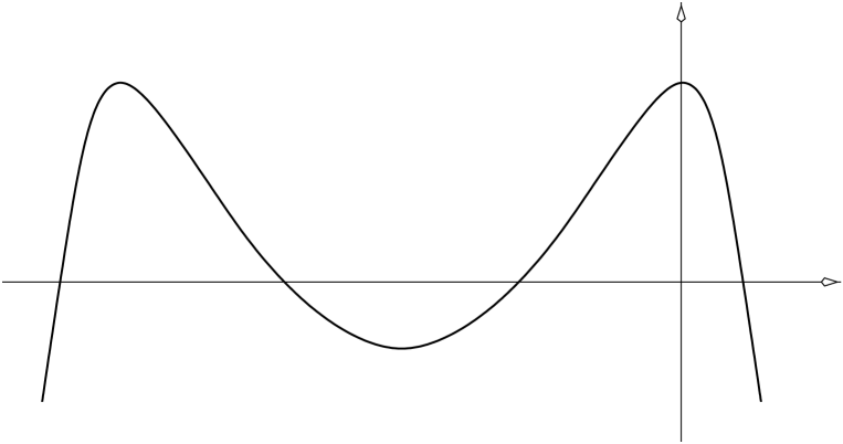
Figure 1: The metric polynomial $p(\xi)$, constrained with the ‘equal temperature condition’ (2.8).

Potential conical singularities exist along the axes $x=\xi_{3}$ and $x=\xi_{4}$. Conventionally the singularity between the black holes (along $\xi_{4}$) is removed by insisting periodicity in the azimuthal coordinate such that

$$\Delta\varphi=\frac{4\pi}{|p^{\prime}(\xi_{4})|},$$ (2.6)

which unavoidably produces a conical deficit along $x=\xi_{3}$. In the C metric this is generally interpreted as a cosmic string lying along the axis and terminating on the black hole. The deficit can be removed by introducing an external gauge field [7] – the Ernst solution, but the Lorentzian section of this metric is no longer asymptotically flat.

The Euclidian section of the C metric may be obtained in the conventional manner by setting $t=i\tau$ in equation (2.1), where in addition the $y$ coordinate must be restricted to the range $y\in[\xi_{2},\xi_{3}]$ to ensure the metric is positive definite. Further potential conical singularities then arise at $y=\xi_{2}$ and $y=\xi_{3}$ which must both be eliminated in order that the metric be regular. This may be achieved [12] by requiring $\tau$ to be periodic, with

$$\Delta\tau=\frac{4\pi}{p^{\prime}(\xi_{3})}$$ (2.7)

and by imposing an additional ‘equal temperature condition’ on $p(\xi)$ such that

$$|p^{\prime}(\xi_{2})|=|p^{\prime}(\xi_{3})|.$$ (2.8)

The latter condition (2.8), only realisable in the electrovac case, may be re-expressed as a relation between the parameters $\eta$ and $\zeta$, or alternatively as equivalent to insisting the roots $\xi_{i}$ of $p(\xi)$ satisfy

$$\xi_{2}-\xi_{1}=\xi_{4}-\xi_{3}.$$ (2.9)

With this regularity condition the topology of the Euclidean section becomes $S^{2}\times S^{2}-\{\mathrm{point}\}$, where the point removed is spatial infinity $x=y=\xi_{3}$.

Of particular relevance to virtual black hole calculations is the ‘point-particle’ limit, in which the black holes are small on scales set by the acceleration. Since an implicit relation holds between $\eta$ and $\zeta$, there exists only one dimensionless parameter in the metric, and so without loss of generality the ‘point-particle’ limit may be expressed as

$$\zeta\ll 1.$$ (2.10)

In this limit deviations from spherical symmetry in the $(x,\varphi)$ section become small, as can be seen by making a coordinate transformation $x\rightarrow\cos\theta$ so that $p(x)=\sin^{2}\theta+\mathcal{O}(\zeta)$. This result evidently has implications for the solution of any ‘angular’ equations for incident fields.

Equation (2.2) may be solved for the roots $\xi_{i}$ which, under the assumption (2.10), can be written as series in $\zeta$ to give

$$\samepage\xi_{1} = -\frac{1}{\zeta}-2+\zeta+\mathcal{O}(\zeta^{2}),$$ (2.11)

$$\xi_{2} = -\frac{1}{\zeta}+\zeta+\mathcal{O}(\zeta^{2}),$$ (2.12)

$$\xi_{3} = -1-\frac{1}{2}\zeta+\mathcal{O}(\zeta^{2}),$$ (2.13)

$$\xi_{4} = 1-\frac{1}{2}\zeta+\mathcal{O}(\zeta^{2}).$$ (2.14)

Clearly then, the acceleration horizon at $y=\xi_{3}$ is largely unaffected by variations in the parameter $\zeta$ if (2.10) holds, whereas the inner and outer black hole horizons $y=\xi_{1}$ and $\xi_{2}$ respectively are both highly sensitive. As $\zeta\rightarrow 0$ these roots $\rightarrow-\infty$ in unison which, together with the identification of infinity at $x=y$, supports the definition of a radial coordinate $r$ [11] as

$$r^{-1}=A\{x-y\}.$$ (2.15)

If the axis $x=\xi_{3}$ is neglected all observers will intersect the acceleration horizon before reaching infinity and, in the ‘point-particle’ limit, the causal structure approaches that shown in figure 2. The surface gravity $\kappa$ at the outer black hole horizon and the acceleration horizon, is given by

$$\kappa\equiv\frac{2\pi}{\Delta\tau}=\frac{p^{\prime}(\xi_{3})}{2}=1-2\zeta+\mathcal{O}(\zeta^{2}).$$ (2.16)

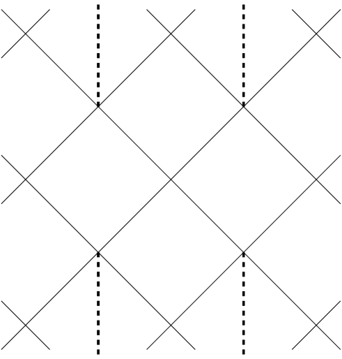
Figure 2: The causal structure of the electrovac C metric in the ‘point-particle’ limit, neglecting the axis $x=\xi_{3}$. The notation follows that of Hawking [5] and Hawking & Ross [8], where $H_{bl}$, $H_{br}$, $H_{al}$ and $H_{ar}$ are the left and right acceleration and outer black hole horizons respectively. The future halves of each are denoted $+$ and the past halves $-$. The heavy dashed lines are curvature singularities at ‘$r=0$’.

Quite apart from the additional conditions placed on the parameters to remove conical singularities and render the Euclidean section regular, the C metric possesses a great deal of intrinsic symmetry which may be suitably exploited in the analysis of incident perturbing fields. In particular, the appropriately normalised null linear combinations of $\xi^{a}$ and $\eta^{a}$ are the repeated principal null vectors of both the Weyl tensor $C_{abcd}$ [11] and the Maxwell tensor $F_{ab}$ [13]. The existence of these repeated null vectors implies the metric is of Petrov type D, and perturbing fields may therefore be treated using the methods first developed by Teukolsky for the Kerr solution.

3 Derivation of the Teukolsky Equation

The C metric and its associated electrovac generalisation are examples of algebraically special spacetimes, – in particular they are of Petrov type $\{2,2\}$ or D which amounts to saying that the Weyl spinor $\Psi_{ABCD}$ may be written as

$$\Psi_{ABCD}=o_{(A}o_{B}\iota_{C}\iota_{D)}$$ (3.1)

for a suitably chosen spin basis $(o,\iota)$. This is equivalent [13] to the existence of two real null vector fields $l$ and $n$, everywhere satisfying

$$l^{b}l^{c}C_{abc[d}l_{e]}=n^{b}n^{c}C_{abc[d}n_{e]}=0.$$ (3.2)

$l$ and $n$ are the repeated principal null vectors of the Weyl tensor $C_{abcd}$ which, for the electrovac solution, coincide with those for the Maxwell tensor so that

$$l^{a}F_{a[b}l_{c]}=n^{a}F_{a[b}n_{c]}=0.$$ (3.3)

For the type D solutions the principal null congruences defined respectively by $l$ and $n$ are both geodesic and shear-free. These conditions are sufficient to guarantee, via the generalised Goldberg-Sachs theorem [14], the existence of a canonical null tetrad $(l,n,m,\overline{m})$ in which the Newman-Penrose spin coefficients $\kappa,\sigma,\lambda,$ and $\nu$ vanish identically, and in which the only non-zero tetrad components of the Weyl and Ricci spinors are $\Psi_{2}$ and $\Phi_{11}$ respectively. In the case of vacuum solutions, $\Phi_{11}$ is also identically zero.

Assuming these results in a vacuum background, Teukolsky [9] combined the Newman-Penrose form of the linearised Ricci and Bianchi identities in pairs to generate decoupled equations satisfied by the first order gravitational perturbations $\Psi_{0}$ and $\Psi_{4}$. By similarly combining the Newman-Penrose form of the Maxwell identities he also found decoupled equations for the tetrad components $\phi_{0}$ and $\phi_{2}$ of a test Maxwell field, and likewise for the tetrad components $\chi_{0}$ and $\chi_{1}$ of a test neutrino field. Introducing a parameter $s$ as the spin-weight [15] of the field components allows the homogeneous form of these equations to be combined and written as

$$\Bigl{\{}[D-(2s-1)\epsilon+\overline{\epsilon}-2s\varrho-\overline{\varrho}](\Delta-2s\gamma+\mu)\Bigr{.}$$ (3.4)

$$-[\delta-(2s-1)\beta+\overline{\pi}-2s\tau-\overline{\alpha}](\overline{\delta}+\pi-2s\alpha)$$

$$\mbox{\hskip 28.45274pt}-\Bigl{.}(2s-1)(s-1)\Psi_{2}\Bigr{\}}\Phi_{s}=0$$

for $s>0$, and

$$\Bigl{\{}[\Delta-(2s+1)\gamma-\overline{\gamma}-2s\mu+\overline{\mu}](D-2s\epsilon-\varrho)\Bigr{.}$$ (3.5)

$$-[\overline{\delta}-(2s+1)\alpha-\overline{\tau}-2s\pi+\overline{\beta}](\delta-2s\beta-\tau)$$

$$\mbox{\hskip 28.45274pt}-\Bigl{.}(2s+1)(s+1)\Psi_{2}\Bigr{\}}\Phi_{s}=0$$

for $s<0$. The $\Phi_{s}$’s are to be interpreted as the tetrad components of the appropriate field, which are conventionally defined as $\Psi_{4}$, $\phi_{2}$ and $\chi_{1}$ for spin-weights -2, -1, and -$\frac{1}{2}$, and $\Psi_{0}$, $\phi_{0}$ and $\chi_{0}$ for spin-weights 2, 1, and $\frac{1}{2}$ respectively.

The above results then also hold for type D electrovac solutions (where $\Phi_{11}\neq 0$) with the exception of $s=\pm 2$, under the assumption that the spin 1 perturbations are not in the background Maxwell field but in another gauge field.

In order to proceed, a choice of tetrad basis $(l,n,m,\overline{m})$ for the C metric must be made. The conventional reality condition on the basis vectors $l$ and $n$ requires that a different choice of tetrad basis be made for the regions in which the metric polynomial $p(y)$ is greater than or less than zero. Dealing first with those regions in which $p(y)>0$, a suitable choice is given by

$$\left.\begin{array}[]{ccr}l_{a}&=&[\sqrt{p(y)},1/\sqrt{p(y)},0,0]\\[2.27621pt] n_{a}&=&[-\sqrt{p(y)},1/\sqrt{p(y)},0,0]\\[2.27621pt] m_{a}&=&[0,0,i/\sqrt{p(x)},-\sqrt{p(x)}]\\ \end{array}\right\}\times\frac{1}{\sqrt{2}A\{x-y\}}.$$ (3.6)

This is the canonical symmetric tetrad, in terms of which the non-zero basis components of the Weyl and Ricci spinors are

$$\Psi_{2}=\frac{1}{12}A^{2}\{x-y\}^{2}[p^{\prime\prime}(x)-p^{\prime\prime}(y)]$$ (3.7)

and

$$\Phi_{11}=-\frac{1}{8}A^{2}\Bigl{(}\{x-y\}^{2}[p^{\prime\prime}(x)+p^{\prime\prime}(y)]\Bigr{.}$$ (3.8)

$$\mbox{\hskip 56.9055pt}\Bigl{.}-2\{x-y\}[p^{\prime}(x)-p^{\prime}(y)]\Bigr{)}$$

respectively. The inherent symmetries of the chosen tetrad force the eight remaining non-zero Newman-Penrose spin coefficients into two real and two complex pairs, so that

$$\samepage-\varrho=\mu = \frac{1}{\sqrt{2}}A\sqrt{p(y)},$$ (3.9)

$$-\gamma=\epsilon = \frac{1}{\sqrt{2p(y)}}A\left\{\frac{1}{2}\{x-y\}p^{\prime}(y)+p(y)\right\},$$ (3.10)

$$\tau=\mbox{}\pi = \frac{i}{\sqrt{2}}A\sqrt{p(x)},$$ (3.11)

$$\alpha=\mbox{}\beta = \frac{i}{\sqrt{2p(x)}}A\left\{\frac{1}{2}\{x-y\}p^{\prime}(x)-p(x)\right\}.$$ (3.12)

Finally, the four directional derivative operators $D$, $\Delta$, $\delta$, and $\overline{\delta}$ become

$$\samepage D = \frac{1}{\sqrt{2}}A\{x-y\}\left(\sqrt{p(y)}\frac{\partial}{\partial y}-\frac{\partial}{\partial t}\right),$$ (3.13)

$$\Delta = \frac{1}{\sqrt{2}}A\{x-y\}\left(\sqrt{p(y)}\frac{\partial}{\partial y}+\frac{\partial}{\partial t}\right),$$ (3.14)

$$\delta = \frac{1}{\sqrt{2}}A\{x-y\}\left(-i\sqrt{p(x)}\frac{\partial}{\partial x}+\frac{\partial}{\partial\varphi}\right),$$ (3.15)

$$\overline{\delta} = \frac{1}{\sqrt{2}}A\{x-y\}\left(i\sqrt{p(x)}\frac{\partial}{\partial x}+\frac{\partial}{\partial\varphi}\right).$$ (3.16)

Substituting the relations (3.7 - 3.16) into equation (3.4), under the assumption that $\Phi_{s}$ is functionally dependent on all coordinates, results in a second order partial differential equation for positive spin-weight fields. This may be combined with the result obtained from a similar substitution into (3.5) and written as

$$A^{2}\Biggl{(}\{x-y\}^{2}\Biggl{[}\frac{1}{2}\partial_{y}\{p(y)\partial_{y}\}-\frac{1}{2p(y)}\left\{\partial_{t}+\frac{1}{2}sp^{\prime}(y)\right\}^{2}-\frac{1}{2}\partial_{x}\{p(x)\partial_{x}\}-\frac{1}{2p(x)}\left\{\partial_{\varphi}+\frac{i}{2}sp^{\prime}(x)\right\}^{2}\Biggr{.}\Biggr{.}$$ (3.17)

$$\Biggl{.}-\frac{1}{12}(2s^{2}+1)\{p^{\prime\prime}(x)-p^{\prime\prime}(y)\}\Biggr{]}+\{x-y\}(|s|+1)\left\{p(y)\partial_{y}+\frac{1}{2}p^{\prime}(y)+p(x)\partial_{x}+\frac{1}{2}p^{\prime}(x)\right\}$$

$$\Biggl{.}\mbox{\hskip 28.45274pt}-\frac{1}{2}(s^{2}+3|s|+2)\{p(x)-p(y)\}\Biggr{)}\Phi_{s}=0$$

which is then valid for massless fields of spin-weight $s=\pm\frac{1}{2}$, $\pm 1$ and $\pm 2$.

For those regions of the C metric in which $p(y)<0$, a suitable choice of tetrad may be obtained from the original with a boost of $-i$ under which the Newman-Penrose quantities $\Psi_{2}$ and $\Phi_{11}$ remain unchanged, the non-zero spin coefficients transform as

$$\begin{array}[]{ccccccc}\tilde{\mu}&=&i\mu,&\mbox{\hskip 28.45274pt}&\tilde{\varrho}&=&-i\varrho,\\ \tilde{\epsilon}&=&-i\epsilon,&\mbox{\hskip 28.45274pt}&\tilde{\gamma}&=&i\gamma,\\ \tilde{\tau}&=&-\tau,&\mbox{\hskip 28.45274pt}&\tilde{\pi}&=&-\pi,\\ \tilde{\alpha}&=&-\alpha,&\mbox{\hskip 28.45274pt}&\tilde{\beta}&=&-\beta,\end{array}$$ (3.18)

and $\Phi_{s}$ acquires a phase factor

$$\Phi_{s}\rightarrow\tilde{\Phi}_{s}=(-i)^{s}\Phi_{s}.$$ (3.19)

Substituting these new relations as before produces identical results to those for the $p(y)>0$ regions, and so the Teukolsky equation (3.17) is valid throughout the C metric solution. Also, by setting $s=0$, the expression reduces to the C metric form of the conformally invariant massless scalar equation

$$\left\{\Box-\frac{1}{6}R\right\}\Phi_{0}=0,$$ (3.20)

and so the domain of definition may be extended to include null scalar fields. Equation (3.17) may therefore be interpreted as describing massless fields of spin-weight $s=0$, $\pm\frac{1}{2}$, $\pm 1$ and $\pm 2$ incident upon the vacuum C metric. In addition, it remains valid in the electrovac C metric when restricted to massless test fields of spin-weight $0$, $\pm\frac{1}{2}$ and $\pm 1$.

The form of equation (3.17) again highlights the inherent symmetries of the chosen tetrad which effectively produce terms in matched pairs – one in $x$ and one in $y$. It is hardly surprising therefore that, with a suitably chosen ansatz for $\Phi_{s}$, the equation separates into two ordinary differential equations in the coordinates $x$ and $y$ respectively. Indeed, the algebraically special character of the C metric was suitably exploited in choosing an appropriate tetrad basis for this exact purpose. This separation procedure has been shown to be possible, given a suitably chosen basis, for all type D vacuum metrics by Kamran & McLenaghan [10], and will be explicitly demonstrated for the C metric in the next section.

4 Separation of Variables

Having derived the expressions for arbitrary spin massless perturbations in type D vacuum solutions, Teukolsky demonstrated [9] that for the Kerr metric the equations separated when expressed in a Kinnersley [16] tetrad. In view of the validity of Teukolsky’s methods, Kamran & McLenaghan conjectured that a similar separation could be performed for the entire class of type D vacuum spacetimes. This was subsequently demonstrated for $s=0$, $\pm\frac{1}{2}$, $\pm 1$ and $\pm 2$ in [10].

For the C metric, the nature of the conformal factor $A\{x-y\}$ [17] and the ignorable coordinates $t$ and $\varphi$ in the metric strongly suggest an ansatz of the form

$$\Phi_{s}=[A\{x-y\}]^{|s|+1}\mathrm{e}^{-i(\omega t-m\varphi)}\Theta_{s}(x,y).$$ (4.1)

Since $\varphi$ is a periodic coordinate (2.6), $m$ must be of the form

$$m=m_{0}\frac{|p^{\prime}(\xi_{4})|}{2}=m_{0}\left\{1+2\zeta+\mathcal{O}(\zeta^{2})\right\}$$ (4.2)

where $m_{0}$ is, without loss of generality, a positive integer.

For the $s>0$ fields, acting with the first two operators in the Newman-Penrose form of the Teukolsky equation (3.4) yields

$$\Bigl{\{}\Delta-2s\gamma+\mu\Bigr{\}}\Phi_{s}=\frac{1}{\sqrt{2}}[A\{x-y\}]^{s+2}\mathrm{e}^{-i(\omega t-m\varphi)}\mathcal{L}_{ys_{+}}\Theta_{s}(x,y),$$ (4.3)

and

$$\Bigl{\{}\overline{\delta}-2s\alpha+\pi\Bigr{\}}\Phi_{s}=\frac{1}{\sqrt{2}}[A\{x-y\}]^{s+2}\mathrm{e}^{-i(\omega t-m\varphi)}\mathcal{L}_{xs_{+}}\Theta_{s}(x,y),$$ (4.4)

where the differential operators $\mathcal{L}_{ys_{+}}$ and $\mathcal{L}_{xs_{+}}$ may be written as

$$\samepage\mathcal{L}_{ys_{+}} = \sqrt{p(y)}\frac{\partial}{\partial y}-\frac{1}{\sqrt{p(y)}}\left\{i\omega-\frac{1}{2}sp^{\prime}(y)\right\},$$ (4.5)

$$\mathcal{L}_{xs_{+}} = i\sqrt{p(x)}\frac{\partial}{\partial x}+\frac{i}{\sqrt{p(x)}}\left\{m+\frac{1}{2}sp^{\prime}(x)\right\}.$$ (4.6)

Similarly for the $s<0$ fields, acting on the same ansatz with the first two operators in equation (3.5) gives

$$\Bigl{\{}D-2s\epsilon-\varrho\Bigr{\}}\Phi_{s}=\frac{1}{\sqrt{2}}[A\{x-y\}]^{-s+2}\mathrm{e}^{-i(\omega t-m\varphi)}\mathcal{L}_{ys_{-}}\Theta_{s}(x,y),$$ (4.7)

and

$$\Bigl{\{}\delta-2s\beta-\tau\Bigr{\}}\Phi_{s}=\frac{1}{\sqrt{2}}[A\{x-y\}]^{-s+2}\mathrm{e}^{-i(\omega t-m\varphi)}\mathcal{L}_{xs_{-}}\Theta_{s}(x,y),$$ (4.8)

where now the operators $\mathcal{L}_{ys_{-}}$ and $\mathcal{L}_{xs_{-}}$ take the form

$$\samepage\mathcal{L}_{ys_{-}} = \sqrt{p(y)}\frac{\partial}{\partial y}+\frac{1}{\sqrt{p(y)}}\left\{i\omega-\frac{1}{2}sp^{\prime}(y)\right\},$$ (4.9)

$$\mathcal{L}_{xs_{-}} = -i\sqrt{p(x)}\frac{\partial}{\partial x}+\frac{i}{\sqrt{p(x)}}\left\{m+\frac{1}{2}sp^{\prime}(x)\right\}.$$ (4.10)

These two sets of equations may obviously be combined into a single pair valid for $s=0$, $\pm\frac{1}{2}$, $\pm 1$, and $\pm 2$ by defining

$$\mathcal{L}_{ys}\stackrel{{\scriptstyle\mathrm{def}}}{{=}}\sqrt{p(y)}\frac{\partial}{\partial y}-\frac{|s|}{s}\frac{1}{\sqrt{p(y)}}\left\{i\omega-\frac{1}{2}sp^{\prime}(y)\right\},$$ (4.11)

and

$$\mathcal{L}_{xs}\stackrel{{\scriptstyle\mathrm{def}}}{{=}}i\frac{|s|}{s}\sqrt{p(x)}\frac{\partial}{\partial x}+\frac{i}{\sqrt{p(y)}}\left\{m+\frac{1}{2}sp^{\prime}(x)\right\}.$$ (4.12)

The remaining operators in the Newman-Penrose form of the Teukolsky equations (3.4, 3.5) may be similarly expanded by allowing them to act on a coordinate-dependant function $\Lambda_{s}(t,y,x,\varphi)$ of the form

$$\Lambda_{s}(t,y,x,\varphi)=\mathrm{e}^{-i(\omega t-m\varphi)}\times\Omega_{s}(x,y).$$ (4.13)

For the $s>0$ case this leads to

$$\Bigl{\{}D-(2s-1)\epsilon+\overline{\epsilon}-2s\varrho-\overline{\varrho}\Bigr{\}}\Lambda_{s}=$$ (4.14)

$$\mbox{\hskip 56.9055pt}\mathrm{e}^{-i(\omega t-m\varphi)}\left\{\frac{1}{\sqrt{2}}A\{x-y\}\mathcal{D}_{ys_{+}}+\mathcal{K}_{ys_{+}}\right\}\Omega_{s}(x,y),$$

$$\Bigl{\{}\delta-(2s-1)\beta+\overline{\pi}-2s\tau-\overline{\alpha}\Bigr{\}}\Lambda_{s}=$$ (4.15)

$$\mbox{\hskip 56.9055pt}\mathrm{e}^{-i(\omega t-m\varphi)}\left\{\frac{1}{\sqrt{2}}A\{x-y\}\mathcal{D}_{xs_{+}}+\mathcal{K}_{xs_{+}}\right\}\Omega_{s}(x,y),$$

and for the $s<0$ case

$$\Bigl{\{}\Delta-(2s+1)\gamma+\overline{\gamma}-2s\mu-\overline{\mu}\Bigr{\}}\Lambda_{s}=$$ (4.16)

$$\mbox{\hskip 56.9055pt}\mathrm{e}^{-i(\omega t-m\varphi)}\left\{\frac{1}{\sqrt{2}}A\{x-y\}\mathcal{D}_{ys_{-}}+\mathcal{K}_{ys_{-}}\right\}\Omega_{s}(x,y),$$

$$\Bigl{\{}\overline{\delta}-(2s+1)\alpha+\overline{\tau}-2s\pi-\overline{\beta}\Bigr{\}}\Lambda_{s}=$$ (4.17)

$$\mbox{\hskip 56.9055pt}\mathrm{e}^{-i(\omega t-m\varphi)}\left\{\frac{1}{\sqrt{2}}A\{x-y\}\mathcal{D}_{xs_{-}}+\mathcal{K}_{xs_{-}}\right\}\Omega_{s}(x,y).$$

As for the $\mathcal{L}$ operators, the $\mathcal{D}$’s and $\mathcal{K}$’s may be combined into pairs defined for both positive and negative $s$ which may be written as

$$\samepage\mathcal{D}_{ys} \stackrel{{\scriptstyle\mathrm{def}}}{{=}} \sqrt{p(y)}\frac{\partial}{\partial y}+\frac{|s|}{s}\frac{1}{\sqrt{p(y)}}\left\{i\omega-\frac{1}{2}\left(s-\frac{|s|}{s}\right)p^{\prime}(y)\right\},$$ (4.18)

$$\mathcal{D}_{xs} \stackrel{{\scriptstyle\mathrm{def}}}{{=}} -i\frac{|s|}{s}\sqrt{p(x)}\frac{\partial}{\partial x}+\frac{i}{\sqrt{p(x)}}\left\{m+\frac{1}{2}\left(s-\frac{|s|}{s}\right)p^{\prime}(x)\right\},$$ (4.19)

and

$$\samepage\mathcal{K}_{ys} \stackrel{{\scriptstyle\mathrm{def}}}{{=}} \frac{1}{\sqrt{2}}\frac{|s|}{s}A\sqrt{p(y)}\left\{s+\frac{2|s|}{s}\right\},$$ (4.20)

$$\mathcal{K}_{xs} \stackrel{{\scriptstyle\mathrm{def}}}{{=}} \frac{i}{\sqrt{2}}A\sqrt{p(x)}\left\{s+\frac{2|s|}{s}\right\}.$$ (4.21)

It should be noted at this stage that each of the $\mathcal{L}$’s, $\mathcal{D}$’s and $\mathcal{K}$’s are functions of only one coordinate, – either $x$ or $y$. If these results are combined appropriately then, given the form of the ansatz (4.1), the Teukolsky equations (3.4) and (3.5) are seen to be wholly equivalent to the single expression

$$\Bigg{(}\left\{\frac{1}{\sqrt{2}}A\{x-y\}\mathcal{D}_{ys}+\mathcal{K}_{ys}\right\}\left[\frac{1}{\sqrt{2}}[A\{x-y\}]^{|s|+2}\mathcal{L}_{ys}\right]\Biggr{.}$$ (4.22)

$$-\left\{\frac{1}{\sqrt{2}}A\{x-y\}\mathcal{D}_{xs}+\mathcal{K}_{xs}\right\}\left[\frac{1}{\sqrt{2}}[A\{x-y\}]^{|s|+2}\mathcal{L}_{xs}\right]$$

$$\Biggl{.}\mbox{\hskip 42.67912pt}-(2|s|-1)(|s|-1)[A\{x-y\}]^{|s|+1}\Psi_{2}\Biggr{)}\Theta_{s}(x,y)=0.$$

Considering the action of both $\mathcal{D}_{ys}$ and $\mathcal{D}_{xs}$ on the term $[A\{x-y\}]^{|s|+2}$ and the explicit form of $\Psi_{2}$ (3.7) this may be substantially simplified, becoming

$$\Bigl{(}\{\mathcal{D}_{ys}\mathcal{L}_{ys}+\frac{1}{6}(2s^{2}-3|s|+1)p^{\prime\prime}(y)\}\ \Bigr{.}$$ (4.23)

$$\Bigl{.}\mbox{\hskip 14.22636pt}-\{\mathcal{D}_{xs}\mathcal{L}_{xs}+\frac{1}{6}(2s^{2}-3|s|+1)p^{\prime\prime}(x)\}\Bigr{)}\Theta_{s}(x,y)=0$$

which is clearly separable under the assumption $\Theta_{s}(x,y)=\phi_{s}(x)\times\psi_{s}(y)$. By expanding the $\mathcal{D}$ and $\mathcal{L}$ operators, the separated expression for the $y$-coordinate may be written as

$$\left(\frac{\partial}{\partial y}\left\{p(y)\frac{\partial}{\partial y}\right\}+\frac{1}{p(y)}\left\{\omega+\frac{i}{2}sp^{\prime}(y)\right\}^{2}+\frac{1}{6}(2s^{2}+1)p^{\prime\prime}(y)+\Gamma_{s}\right)\psi_{s}(y)=0$$ (4.24)

where $\Gamma_{s}$ is a separation constant which will in general depend on the spin-weight $s$. Likewise for the $x$-coordinate, the separated equation becomes

$$\left(\frac{\partial}{\partial x}\left\{p(x)\frac{\partial}{\partial x}\right\}-\frac{1}{p(x)}\left\{m+\frac{1}{2}sp^{\prime}(x)\right\}^{2}+\frac{1}{6}(2s^{2}+1)p^{\prime\prime}(x)+\Gamma_{s}\right)\phi_{s}(x)=0.$$ (4.25)

The pair of separated equations (4.24) and (4.25) may be said to describe the $y$ and $x$ components respectively of fields with all spin-weights considered incident on the vacuum C metric. As before, they continue to hold in the electrovac C metric if restricted to massless test fields of spin-weight $s=0$, $\pm\frac{1}{2}$ and $\pm 1$.

The unification and subsequent separation of the equations describing incident fields of a variety of spin-weights evidently represents an appreciable success for the Newman-Penrose formalism. However the resulting expressions, when considered as a pair of second order ordinary differential equations, are seen to possess five regular singular points – the four roots of $p(\xi)$ and $\infty$ – and hence cannot be solved analytically. In order to furnish even an approximate solution, the ‘point-particle’ limit must be exploited to suitably simplify both equations.

5 Solving the $x$ Equation

Equation (4.25) for $\phi_{s}(x)$, together with suitable conditions of regularity at the boundaries $x=\xi_{3}$ and $\xi_{4}$ represents a Sturm-Liouville eigenvalue problem for the separation constant $\Gamma_{s}$. For fixed $s$ and $m$ the eigenvalues may be labelled by $j$, where it is assumed that

$$j=j_{0}+\zeta j_{1}+\mathcal{O}(\zeta^{2}).$$ (5.1)

Since the expression is self-adjoint, its eigenfunctions – labelled by $s$, $m$ and $j$, – will be both complete and orthogonal on the interval $x\in[\xi_{3},\xi_{4}]$, but the existence of five regular singular points implies these solutions will not have a closed form in terms of known functions. However, considerable analytic progress may be made by moving to the ‘point-particle’ limit after first changing variables

$$x\rightarrow\hat{x}=\frac{1}{\beta}\left(x-\frac{1}{2}\{\xi_{3}+\xi_{4}\}\right)$$ (5.2)

where

$$\beta\stackrel{{\scriptstyle\mathrm{def}}}{{=}}\frac{1}{2}\{\xi_{4}-\xi_{3}\}.$$ (5.3)

The range of $x$ is then mapped to $\hat{x}\in[-1,1]$, and the metric polynomial may be re-written as

$$p(\hat{x})=-\eta\zeta\beta^{4}\Bigl{\{}(\hat{x}+\alpha)^{2}-1\Bigr{\}}\Bigl{\{}\hat{x}^{2}-1\Bigr{\}}$$ (5.4)

with

$$\alpha\stackrel{{\scriptstyle\mathrm{def}}}{{=}}\frac{1}{\beta}\left\{\xi_{3}-\xi_{1}\right\}.$$ (5.5)

Having made this change, equation (4.25) becomes

$$\left(\frac{1}{\beta^{2}}\frac{\partial}{\partial\hat{x}}\left\{p(\hat{x})\frac{\partial}{\partial\hat{x}}\right\}-\frac{1}{p(\hat{x})}\left\{m+\frac{1}{2}sp^{\prime}(\hat{x})\right\}^{2}+\frac{1}{6}(2s^{2}+1)p^{\prime\prime}(\hat{x})+\Gamma_{s}\right){{}_{s}\phi_{jm}}(\hat{x})=0$$ (5.6)

where ^′ denotes differentiation with respect to $x$, and $\partial_{\hat{x}}=\beta\partial_{x}$.

In the limit $\zeta\ll 1$ the three polynomials $p(\hat{x})$, $p^{\prime}(\hat{x})$ and $p^{\prime\prime}(\hat{x})$ may be expressed as power series in $\zeta$

$$\samepage p(\hat{x}) = (1-\hat{x}^{2})\bigg{\{}1+2\hat{x}\zeta+\mathcal{O}(\zeta^{2})\bigg{\}},$$ (5.7)

$$p^{\prime}(\hat{x}) = -2\bigg{\{}\hat{x}-(1-3\hat{x}^{2})\zeta+\mathcal{O}(\zeta^{2})\bigg{\}},$$ (5.8)

$$p^{\prime\prime}(\hat{x}) = -2\bigg{\{}1+6\hat{x}\zeta+\mathcal{O}(\zeta^{2})\bigg{\}}.$$ (5.9)

If it is further assumed that the eigenfunctions may also be written as a power series in $\zeta$

$${{}_{s}^{\phantom{0}}\phi_{jm}^{\phantom{0}}}={{}_{s}^{\phantom{0}}\phi_{jm}^{(0)}}+{{}_{s}^{\phantom{1}}\phi_{jm}^{(1)}}\zeta+\mathcal{O}(\zeta^{2})$$ (5.10)

then (5.6) may be separated into a series of equations for these individual functions, the first of which is

$$\left(\frac{\partial}{\partial\hat{x}}\left\{(1-\hat{x}^{2})\frac{\partial}{\partial\hat{x}}\right\}-\frac{\left\{m_{0}-s\hat{x}\right\}^{2}}{1-\hat{x}^{2}}-\frac{1}{3}(2s^{2}+1)+\Gamma_{s}\right){{}_{s}^{\phantom{0}}\phi_{jm}^{(0)}}(\hat{x})=0.$$ (5.11)

If the label $j$ is defined via the equation

$$\Gamma_{s}=j(j+1)-\frac{1}{3}(s^{2}-1)$$ (5.12)

then, with an additional change of variables $\hat{x}\rightarrow-\cos\theta$, this reduces to

$$\left(\frac{1}{\sin\theta}\frac{\partial}{\partial\theta}\left\{\sin\theta\frac{\partial}{\partial\theta}\right\}-\left\{\frac{m_{0}+s\cos\theta}{\sin\theta}\right\}^{2}-s^{2}+j_{0}(j_{0}+1)\right){{}_{s}^{\phantom{0}}\phi_{jm}^{(0)}}(\theta)=0.$$ (5.13)

Since the zeroth order in $\zeta$ corresponds to a limit of spherical symmetry in the $(\theta,\varphi)$ section it is hardly surprising that the solutions are related to the spin-weighted spherical harmonics [18]

$${{}_{s}^{\phantom{0}}Y_{jm}^{\phantom{0}}}(\theta,\varphi)={{}_{s}^{\phantom{0}}\phi_{jm}^{(0)}}(\theta)\times\mathrm{e}^{im\varphi}.$$ (5.14)

$j_{0}$ must therefore be half-integer, satisfying $j_{0}\geq\mathrm{max}(|m_{0}|,|s|)$ – so in this limit $j_{0}$ and $m_{0}$ are the usual ‘total angular momentum’ and ‘angular momentum about the symmetry axis’ quantum numbers respectively.

Strictly this derivation has assumed the relation implicit between the parameters $\eta$ and $\zeta$ of the metric due to the imposed ‘equal temperature condition’ (2.8). In this sense the solutions to (4.25), expressed in the ‘point-particle’ limit as

$$\phi_{s}(x)={}_{s}\phi_{jm}(\theta)=\mathrm{e}^{-im\varphi}\times{}_{s}Y_{jm}(\theta,\varphi)+\mathcal{O}(\zeta)$$ (5.15)

describe the $x$ component of massless test fields of spin-weight $s=0$, $\pm\frac{1}{2}$ and $\pm 1$ only, incident on the electrovac C metric. This is the desired result for virtual black hole calculations, but for the sake of completeness, to zeroth order in $\zeta$ the metric polynomial and its derivatives are identical in the vacuum ($\eta\equiv 0$) case, and so (5.15) is in addition valid for all spin-weights incident on the vacuum C metric.

6 Boundary Conditions on the $y$ Equation.

The evolution of fields with spin-weight $s$ described by equation (4.24) essentially defines a one-dimensional scattering problem, upon which suitable asymptotic boundary conditions must be imposed in order that the problem be well-defined. Following Hawking & Ross [8], initial data for the incident fields may be defined on an ‘initial’ Cauchy surface suitably constructed from the left acceleration and right black hole horizons. The scattering problem then becomes the propagation of this data forward through the spacetime to a ‘future’ Cauchy surface constructed from the future halves of the left and right black hole horizons and $\mathcal{J}^{+}$. The form of the initial data on the acceleration and black hole horizons is nonetheless restricted by the behaviour of the fields as the metric polynomial $p(y)\rightarrow 0$, since it is in this limit that the horizons are approached.

With the exception of fields incident along the axis $x=\xi_{3}$ this problem may conveniently be divided into two sections – propagation from $H_{al}^{-}$ and $H_{br}^{-}$ to $H_{ar}^{+}$ and $H_{bl}^{+}$, followed by propagation from $H_{ar}^{+}$ and $H_{al}^{+}$ to $\mathcal{J}^{+}$. The axially incident portion of the field is an exceptional case since this is the unique component which reaches $\mathcal{J}^{+}$ before intersecting the acceleration horizon. However this contribution may consistently be disregarded as a set of measure zero amongst the entirety of the incident field.

Further insight into the asymptotic behaviour of equation (4.24) may be gained by defining a conventional ‘tortoise’ coordinate $y_{*}$ such that

$$dy_{*}=-\frac{dy}{p(y)}.$$ (6.1)

Since $p(\xi_{i})=0$, the range $y_{*}\in(-\infty,\infty)$ covers only the region between two horizons, and therefore a separate $(t,y_{*},x,\varphi)$ coordinate system is required for each ‘Rindler diamond’ in the spacetime (figure 3). Attention will be focused on the first half of the scattering problem – propagation through a single Rindler diamond from $H_{al}^{-}$ and $H_{br}^{-}$ to $H_{ar}^{+}$ and $H_{bl}^{+}$. The second half is subsequently found to be trivial.

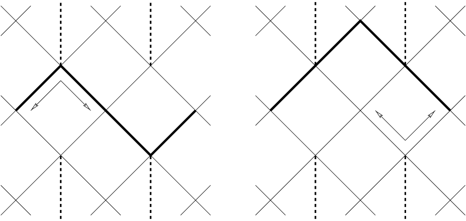
Figure 3: Penrose diagrams for the electrovac C metric showing the initial and future Cauchy surfaces respectively, and the null coordinates $u,v=t\mp y_{*}$ in two ‘Rindler diamonds’.

Using the form of the metric polynomial given in equation (2.5) the coordinate $y_{*}$ may be written as

$$\samepage y_{*} = \frac{1}{\eta\zeta}\int\frac{dy}{\{y-\xi_{1}\}\{y-\xi_{2}\}\{y-\xi_{3}\}\{y-\xi_{4}\}}$$ (6.2)

$$= -\gamma_{1}\ln|\xi_{1}-y|+\gamma_{2}\ln|\xi_{2}-y|-\gamma_{3}\ln|\xi_{3}-y|+\gamma_{4}\ln|\xi_{4}-y|$$

where the $\gamma_{i}$ are constant positive functions of the four roots $\xi_{i}$. In the ‘point-particle’ limit, they become

$$\gamma_{i}=\frac{1}{2}\pm\zeta+\mathcal{O}(\zeta^{2}),$$ (6.3)

with a ‘$-$’ for $i=1$ and $4$ and a ‘$+$’ for $i=2$ and $3$. Clearly then, $y_{*}\rightarrow\infty$ at the acceleration and inner black hole horizons, and $y_{*}\rightarrow-\infty$ at the outer black hole horizon.

Multiplying through by $p(y)$ and further recognising $\partial_{y_{*}}=-p(y)\partial_{y}$ allows equation (4.24) to be re-written as the one-dimensional wave equation

$$\left(\frac{\partial^{2}}{\partial y_{*}^{2}}+\left\{\omega+\frac{i}{2}sp^{\prime}(y)\right\}^{2}+V_{\mathrm{eff}}\right)\psi_{s}(y)=0$$ (6.4)

where the effective potential is given by

$$V_{\mathrm{eff}}=p(y)\left\{\frac{1}{6}(2s^{2}+1)p^{\prime\prime}(y)+\Gamma_{s}\right\}.$$ (6.5)

Near the outer black hole horizon $p(y)\rightarrow 0$ and hence the effective potential becomes negligibly small. In addition $p^{\prime}(y)\rightarrow-2\kappa$ where $\kappa$ is the surface gravity of the horizon, and so the solution approaches

$$\left.\psi_{s}(y)\right|_{y\rightarrow\xi_{2}}\sim\mathrm{e}^{\pm i\{\omega-is\kappa\}y_{*}}.$$ (6.6)

Similarly, near the acceleration horizon $p^{\prime}(y)\rightarrow 2\kappa$, and so the solution there approaches

$$\left.\psi_{s}(y)\right|_{y\rightarrow\xi_{3}}\sim\mathrm{e}^{\pm i\{\omega+is\kappa\}y_{*}}.$$ (6.7)

It is clear that for some values of $s\neq 0$ the asymptotic limits of these solutions are unbounded due to terms of the form $\mathrm{e}^{\pm s\kappa y_{*}}$. Such singularities are of course not physical, but instead are due to the fact that the terms $\psi_{s}(y)$ are Newman-Penrose quantities, and hence projections of some physical quantity onto a tetrad which is ill-defined at the horizons. They are therefore gauge- or frame-dependent. This effect may be illustrated by re-expressing the tetrad in null coordinates and subsequently applying a position dependent boost to demonstrate that certain ‘well behaved’ observers at the horizons will not witness such pathology in all of the field quantities.

In ingoing coordinates $(v,r,x,\varphi)$ defined via the relations

$$dv=\frac{1}{A}\{dt+dy_{*}\}$$ (6.8)

for the null coordinate, and

$$dr=-\frac{1}{A\{x-y\}^{2}}\{p(y)dy_{*}+dx\}$$ (6.9)

for the radial coordinate (2.15), the $l$ and $n$ tetrad components may be written as

$$l^{a}=[\{x-y\}\Lambda,\{x-y\}^{-1}\Lambda^{-1},0,0]\qquad\mbox{and}\qquad n^{a}=[0,-\{x-y\}^{-1}\Lambda^{-1},0,0]$$ (6.10)

where

$$\Lambda=i\sqrt{2/p(y)}.$$ (6.11)

Both components remain singular at $p(y)=0$, but by applying a boost $\Lambda^{-1}$ they become [14]

$$l^{a}=[\{x-y\},\{x-y\}^{-1}\Lambda^{-2},0,0]\qquad\mbox{and}\qquad n^{a}=[0,-\{x-y\}^{-1},0,0]$$ (6.12)

which are evidently ‘well behaved’ at the horizons.

The effect of this boost is to transform the Newman-Penrose quantities according to the relation

$$\psi_{s}^{\mathrm{in}}(y)=\Lambda^{-s}\psi_{s}(y),$$ (6.13)

for which the $y$ equation becomes

$$\Bigg{(}{\partial\over\partial y}\left\{p(y){\partial\over\partial y}\right\}-sp^{\prime}(y){\partial\over\partial y}+{1\over p(y)}\{\omega^{2}+i\omega sp^{\prime}(y)\}$$ (6.14)

$$\hskip 71.13188pt+{1\over 6}(2s^{2}-3s+1)p^{\prime\prime}(y)+\Gamma_{s}\Bigg{)}\psi_{s}^{\mathrm{in}}(y)=0.$$

The asymptotic form of this equation may once again be obtained with multiplication through by $p(y)$ to yield

$$\left({\partial^{2}\over\partial y_{*}^{2}}+sp^{\prime}(y){\partial\over\partial y_{*}}+\{\omega^{2}+i\omega sp^{\prime}(y)\}+\hat{V}_{\mathrm{eff}}\right)\psi_{s}^{\mathrm{in}}(y)=0,$$ (6.15)

the solutions to which are

$$\left.\psi_{s}^{\mathrm{in}}(y)\right|_{y\rightarrow\xi_{2}}\sim\mathrm{e}^{-i\omega y_{*}}\mbox{\hskip 5.69054pt or \hskip 7.11317pt}\mathrm{e}^{\{i\omega+2s\kappa\}y_{*}}$$ (6.16)

and

$$\left.\psi_{s}^{\mathrm{in}}(y)\right|_{y\rightarrow\xi_{3}}\sim\mathrm{e}^{-i\omega y_{*}}\mbox{\hskip 5.69054pt or \hskip 7.11317pt}\mathrm{e}^{\{i\omega-2s\kappa\}y_{*}}.$$ (6.17)

In outgoing coordinates $(u,r,x,\varphi)$ where $u$ is defined by

$$du=\frac{1}{A}\{dt-dy_{*}\},$$ (6.18)

the tetrad components $l$ and $n$ are rendered ‘well behaved’ at the horizons by applying a boost of $\Lambda$, the effect of which is to transform the Newman-Penrose quantities according to

$$\psi_{s}^{\mathrm{out}}(y)=\Lambda^{s}\psi_{s}(y).$$ (6.19)

In this case the asymptotic form of the $y$ equation is given by

$$\left({\partial^{2}\over\partial y_{*}^{2}}-sp^{\prime}(y){\partial\over\partial y_{*}}+\{\omega^{2}+i\omega sp^{\prime}(y)\}+\tilde{V}_{\mathrm{eff}}\right)\psi_{s}^{\mathrm{out}}(y)=0,$$ (6.20)

such that

$$\left.\psi_{s}^{\mathrm{out}}(y)\right|_{y\rightarrow\xi_{2}}\sim\mathrm{e}^{i\omega y_{*}}\mbox{\hskip 5.69054pt or \hskip 7.11317pt}\mathrm{e}^{\{-i\omega+2s\kappa\}y_{*}}$$ (6.21)

and

$$\left.\psi_{s}^{\mathrm{out}}(y)\right|_{y\rightarrow\xi_{3}}\sim\mathrm{e}^{i\omega y_{*}}\mbox{\hskip 5.69054pt or \hskip 7.11317pt}\mathrm{e}^{\{-i\omega-2s\kappa\}y_{*}}.$$ (6.22)

The asymptotic behaviour of the field quantities expressed in both the symmetric tetrad and the in- and outgoing tetrads clearly exhibit the peeling behaviour expected from the peeling theorem of Newman & Penrose [19]. Ingoing observers ‘pick out’ the ingoing component of the field to be ‘non-special’ – neither singular nor identically zero at the horizons [9], and likewise the outgoing observers ‘pick out’ the outgoing components. The apparent pathology in some field components is merely a result of some gauge choice, and choosing to work in any particular gauge, with appropriately selected boundary conditions, cannot therefore affect the final results.

Care must nonetheless be exercised when attempting to define certain quantities since $y$ equations such as (4.24) describe the evolution of only a single spin-weight quantity $\psi_{s}(y)$. The failure of these equations to be self-adjoint in cases other than $s=0$ is manifested as an apparent lack of unitarity in the evolution of any one spin-weight component. However, for fields with $s\neq 0$ there must also exist relations between the components of maximum spin-weight – the Teukolsky-Starobinsky identities [20], and consequently the definitions of quantities such as conserved currents must necessarily involve both spin-weight components of a field [21].

Having laid the groundwork, the definition of asymptotic boundary conditions for the desired scattering problem may be achieved by analogy with a simple one-dimensional problem of scattering in a potential well. Considering the initial hypersurfaces $H_{br}^{-}$ and $H_{al}^{-}$, Hawking & Ross argued [8] that the effects of scattering a field from $H_{br}^{-}$ must be the image under left-right interchange to the effects of scattering a field from $H_{al}^{-}$. Since the metric must be symmetric under this exchange, calculating the scattering of a field incident only from the past black hole horizon is justified since the reflection and transmission coefficients would be identical had the other choice been made instead.

With this in mind, an asymptotically-plane wave outgoing from $H_{br}^{-}$ will propagate through the right Rindler diamond and subsequently interact with some potential in the interior region. The result of this interaction must then be an ingoing reflected component through $H_{bl}^{+}$ and an outgoing transmitted component across $H_{ar}^{+}$. These conditions may be written in symmetric tetrad components as

$$\psi_{s}(y)=\mathrm{e}^{\{i\omega+s\kappa\}y_{*}}+C_{R}(s)\mathrm{e}^{\{-i\omega-s\kappa\}y_{*}}$$ (6.23)

at the black hole horizon ($y_{*}\rightarrow-\infty$), and

$$\psi_{s}(y)=C_{T}(s)\mathrm{e}^{\{i\omega-s\kappa\}y_{*}}$$ (6.24)

at the acceleration horizon ($y_{*}\rightarrow\infty$), where $C_{R}(s)$ and $C_{T}(s)$ are related to the reflection and transmission coefficients respectively, which remain to be determined. For the degenerate case of $s=0$, the boundary conditions reduce to those chosen for the massless scalar field in Hawking & Ross, although the ‘tortoise’ coordinate is there defined with opposite sign.

7 Solving the $y$ Equation.

Having established physically consistent boundary conditions at the horizons, the remaining problem of determining the reflection and transmission coefficients reduces to that of solving (4.24) subject to the constraints (6.23) and (6.24). Since this expression possesses the same regular singular points encountered in the $x$ equation, attempting to find an analytic solution will obviously necessitate recourse to the now familiar ‘point-particle’ limit.

Defining a new field $f_{s}(y)$ such that

$$\psi_{s}(y)=\mathrm{e}^{\{i\omega-s\kappa\}y_{*}}f_{s}(y)$$ (7.1)

yields a slightly more pellucid form for this problem, in which (4.24) may be re-written as

$$\Bigg{(}\frac{\partial}{\partial y}\left\{p(y)\frac{\partial}{\partial y}\right\}-2\left\{i\omega-s\kappa\right\}\frac{\partial}{\partial y}+\frac{1}{6}(2s^{2}+1)p^{\prime\prime}(y)+\Gamma_{s}$$ (7.2)

$$\mbox{\hskip 28.45274pt}+\frac{1}{p(y)}\left\{(i\omega-s\kappa)^{2}-(i\omega-\frac{1}{2}sp^{\prime}(y))^{2}\right\}\Bigg{)}f_{s}(y)=0.$$

The boundary conditions then become

$$f_{s}(y)=\mathrm{e}^{2s\kappa y_{*}}+C_{R}(s)\mathrm{e}^{-2i\omega y_{*}}$$ (7.3)

at the black hole horizon ($y_{*}\rightarrow-\infty$), and

$$f_{s}(y)=C_{T}(s)$$ (7.4)

at the acceleration horizon ($y_{*}\rightarrow\infty$).

In moving to the ‘point-particle’ limit this equation is further simplified by changing coordinates

$$y\rightarrow\hat{y}=\frac{1}{\beta}\left(y-\frac{1}{2}\{\xi_{3}+\xi_{2}\}\right)$$ (7.5)

where

$$\beta\stackrel{{\scriptstyle\mathrm{def}}}{{=}}\frac{1}{2}\{\xi_{3}-\xi_{2}\}=\frac{1}{2\zeta}\{1+\zeta+\mathcal{O}(\zeta^{2})\}.$$ (7.6)

The range of $y$ is then mapped to $\hat{y}\in[-1,1]$, and the symmetry imposed on the metric polynomial allows it to be re-written as

$$p(\hat{y})=-\eta\zeta\beta^{4}\{\hat{y}^{2}-\alpha^{2}\}\{\hat{y}^{2}-1\}$$ (7.7)

with

$$\alpha\stackrel{{\scriptstyle\mathrm{def}}}{{=}}\frac{\xi_{4}-\xi_{1}}{\xi_{3}-\xi_{2}}=1+4\zeta+\mathcal{O}(\zeta^{2}).$$ (7.8)

With this change in place the three polynomial functions $p(y)$, $p^{\prime}(y)$ and $p^{\prime\prime}(y)$ – where ^′ denotes differentiation with respect to $y$ – may be expressed as power series in $\zeta$ which are respectively

$$\samepage p(\hat{y}) = -\frac{1}{16\zeta^{2}}(1-\hat{y}^{2})\bigg{\{}(1-\hat{y}^{2})+2(1+3\hat{y}^{2})\zeta+\mathcal{O}(\zeta^{2})\bigg{\}},$$ (7.9)

$$p^{\prime}(\hat{y}) = \frac{1}{2\zeta}\hat{y}\bigg{\{}(1-\hat{y}^{2})-(1-5\hat{y}^{2})\zeta+\mathcal{O}(\zeta^{2})\bigg{\}},$$ (7.10)

$$p^{\prime\prime}(\hat{y}) = \bigg{\{}(1-3\hat{y}^{2})+12\hat{y}^{2}\zeta+\mathcal{O}(\zeta^{2})\bigg{\}}.$$ (7.11)

If $(\hat{y}^{2}-1)\sim\mathcal{O}(1)$ then only the first terms in these series need be retained. Substituting them into (7.2) with the identification (5.12) for $\Gamma_{s}$, and further assuming $\omega\sim\mathcal{O}(1)$ gives

$$\left(\frac{\partial}{\partial\hat{y}}\left\{(\hat{y}^{2}-1)^{2}\frac{\partial}{\partial\hat{y}}\right\}+2\left\{\hat{y}^{2}-[1+2j(j+1)]\right\}\right)f_{s}(\hat{y})=0$$ (7.12)

where $\partial_{\hat{y}}=\beta\partial_{y}$. In this approximate equation $j$ is used in favour of $j_{0}$ since regarding $j$ as a half-integer would introduce degeneracies that are not present in the exact equation. The solution may be expressed in the form

$$f_{s}(\hat{y})=\frac{1}{\{\hat{y}^{2}-1\}^{j+1}}\left\{A\{\hat{y}+1\}^{2j+1}+B\{\hat{y}-1\}^{2j+1}\right\}$$ (7.13)

for arbitrary constants $A$ and $B$. Clearly this function diverges at the boundaries $\hat{y}=\pm 1$, but this is of little real concern since (7.12) is not valid near those points. A separate approximation must therefore be used in the neighbourhoods of the boundaries, which may be obtained by defining a new coordinate $q$ where

$$\hat{y}=\pm\{1-4\zeta q\}.$$ (7.14)

Dealing first with the neighbourhood of $\hat{y}=-1$, the leading order terms in equation (7.2) become

$$\left(\frac{\partial}{\partial q}\left\{q(q+1)\frac{\partial}{\partial q}\right\}+\{i\omega-s\}\frac{\partial}{\partial q}-\frac{i\omega s}{q}-j(j+1)\right)f_{s}(q)=0.$$ (7.15)

Searching for a series solution of the form $f_{s}(q)=\sum a_{\lambda}q^{k+\lambda}$ yields indicial roots $k=+s$ and $-i\omega$, and a general one-term recurrence relation of the form

$$a_{n+1}=a_{n}\left\{\frac{j(j+1)-(k+n)(k+n+1)}{(k+n+1)[k+n+i\omega-s+1]-i\omega s}\right\}.$$ (7.16)

This may be identified as a ${{}_{2}F_{1}}$ Gaussian hypergeometric series, convergent throughout the unit disk $|q|<1$ for the non-integer parameters considered here. The solution obeying the boundary condition (7.3) is therefore

$$f_{s}(q)=\{4\zeta q\}^{s}F\Big{(}\{j+s+1\},\{-j+s\};\{i\omega+s+1\};-q\Big{)}$$ (7.17)

$$\mbox{\hskip 42.67912pt}+C_{R}(s)\{4\zeta q\}^{-i\omega}F\Big{(}\{j-i\omega+1\},\{-j-i\omega\};\{-s-i\omega+1\};-q\Big{)}.$$

Moving to the neighbourhood of $\hat{y}=+1$, the leading-order terms in equation (7.2) now give

$$\left(\frac{\partial}{\partial q}\left\{q(q+1)\frac{\partial}{\partial q}\right\}-\{i\omega-s\}\frac{\partial}{\partial q}+\frac{i\omega s}{q+1}-j(j+1)\right)f_{s}(q)=0.$$ (7.18)

Written in this form an attempted series solution generates a two-term recurrence relation which is of little use. However, a one-term relation may be generated by instead considering the coordinate $\tilde{q}\stackrel{{\scriptstyle\mathrm{def}}}{{=}}q+1$. In this case

$$\left(\frac{\partial}{\partial\tilde{q}}\left\{\tilde{q}(\tilde{q}-1)\frac{\partial}{\partial\tilde{q}}\right\}-\{i\omega-s\}\frac{\partial}{\partial\tilde{q}}+\frac{i\omega s}{\tilde{q}}-j(j+1)\right)f_{s}(\tilde{q}-1)=0$$ (7.19)

which again gives indicial roots of $k=+s$ and $-i\omega$, but with a general recurrence relation of the form

$$a_{n+1}=a_{n}\left\{\frac{(k+n)(k+n+1)-j(j+1)}{(k+n+1)[k+n+i\omega-s+1]-i\omega s}\right\}.$$ (7.20)

Naturally this may also be identified as a ${{}_{2}F_{1}}$ Gaussian hypergeometric series, and the general solution for $f_{s}(q)$ may be expressed as

$$\{q+1\}^{-s}f_{s}(q)=CF\Big{(}\{j+s+1\},\{-j+s\};\{i\omega+s+1\};q+1\Big{)}$$ (7.21)

$$\mbox{\hskip 42.67912pt}+D\{q+1\}^{-s-i\omega}F\Big{(}\{j-i\omega+1\},\{-j-i\omega\};\{-s-i\omega+1\};q+1\Big{)}$$

for arbitrary constants $C$ and $D$. If these are chosen respectively as

$$\samepage C = C_{T}(s)\times\frac{\Gamma(s-i\omega+1)\Gamma(-s-i\omega)}{\Gamma(-j-i\omega)\Gamma(j-i\omega+1)}$$ (7.22)

$$D = C_{T}(s)\times\frac{\Gamma(s-i\omega+1)\Gamma(s+i\omega)}{\Gamma(-j+s)\Gamma(j+s+1)},$$ (7.23)

then (7.21) may be transformed (see for example [22]) to a solution of the form

$$f_{s}(q)=C_{T}(s)\{q+1\}^{s}F\Big{(}\{j+s+1\},\{-j+s\};\{s-i\omega+1\};-q\Big{)}$$ (7.24)

which clearly satisfies the boundary condition (7.4).

At this stage it should be noted that equation (7.18) and its solution (7.24) will also be valid for the entire region $\hat{y}\in[1,\alpha]$. To zeroth order this solution therefore describes the form of the incident field with the desired boundary condition on $H_{ar}^{+}$, restricted to zero on $H_{al}^{+}$ , through the top Rindler diamond bounded by $\mathcal{J}^{+}$. $C_{T}(s)$ is therefore related to the transmission coefficient for the complete scattering problem from the previously defined initial Cauchy surface to the future Cauchy surface.

8 Transmission and Reflection Coefficients

Although the definition of the Gaussian hypergeometric series ensures its convergence only within the unit disk, there nonetheless exist transformation formulae for analytically continuing to the region $|q|>1$ [22]. The boundary neighbourhood solutions (7.17) and (7.24) may therefore be analytically continued to large values of $q$ and subsequently matched to the function (7.13) which is valid in this ‘central’ region.

In the interest of notational convenience, the following factors are defined:

$$\samepage U = \displaystyle{\Gamma(-s-i\omega+1)\Gamma(2j+1)\over\Gamma(j-i\omega+1)\Gamma(j-s+1)},$$ (8.1)

$$V = \displaystyle{\Gamma(s+i\omega+1)\Gamma(j-i\omega+1)\Gamma(j-s+1)\over\Gamma(j+s+1)\Gamma(-s-i\omega+1)\Gamma(j+i\omega+1)},$$ (8.2)

$$W = \displaystyle{\Gamma(s-i\omega+1)\Gamma(-2j-1)\over\Gamma(-j-i\omega)\Gamma(-j+s)},$$ (8.3)

$$X = \displaystyle{\Gamma(-s-i\omega+1)\Gamma(-2j-1)\over\Gamma(-j-i\omega)\Gamma(-j-s)},$$ (8.4)

$$Y = \displaystyle{\Gamma(s+i\omega+1)\Gamma(-j-i\omega)\Gamma(-j-s)\over\Gamma(-j+s)\Gamma(-s-i\omega+1)\Gamma(-j+i\omega)},$$ (8.5)

$$Z = \displaystyle{\Gamma(s-i\omega+1)\Gamma(2j+1)\over\Gamma(j-i\omega+1)\Gamma(j+s+1)},$$ (8.6)

where it is clear from their definitions that, amongst others, the following relations hold:

$$\begin{array}[]{cccccc}U(-s)&=&Z(s),\mbox{\hskip 28.45274pt}&W(-s)&=&X(s),\\[2.27621pt] V^{*}(-s)&=&V^{-1}(s),\mbox{\hskip 28.45274pt}&Y^{*}(-s)&=&Y^{-1}(s).\end{array}$$

With the benefit of these definitions, the analytic continuation of $f_{s}(q)$ from the black hole horizon may be written as

$$f_{s}(q)=X\left(\{4\zeta\}^{-i\omega}C_{R}(s)+\{4\zeta\}^{s}Y\right)\{q\}^{-j-1}$$ (8.7)

$$\mbox{\hskip 56.9055pt}+U\left(\{4\zeta\}^{-i\omega}C_{R}(s)+\{4\zeta\}^{s}V\right)\{q\}^{j}$$

for $q\gg 1$. Likewise the analytic continuation of $f_{s}(q)$ from the acceleration horizon becomes

$$f_{s}(q)=WC_{T}(s)\{q\}^{-j-1}+ZC_{T}(s)\{q\}^{j}.$$ (8.8)

By substituting for the coordinate $q$ defined near $\hat{y}=\pm 1$, equation (7.13) becomes

$$f_{s}(q)\approx\Big{(}\{-1\}^{-j-1}\times 2^{j-1}\times A\times\{\zeta q\}^{j}\Big{)}$$ (8.9)

$$\mbox{\hskip 56.9055pt}+\Big{(}\{-1\}^{j}\times 2^{-j-2}\times B\times\{\zeta q\}^{-j-1}\Big{)}$$

by the black hole horizon, and

$$f_{s}(q)\approx\Big{(}\{-1\}^{-j-1}\times 2^{-j-2}\times A\times\{\zeta q\}^{-j-1}\Big{)}$$ (8.10)

$$\mbox{\hskip 71.13188pt}+\Big{(}\{-1\}^{j}\times 2^{j-1}\times B\times\{\zeta q\}^{j}\Big{)}$$

by the acceleration horizon. Matching these results with the corresponding analytically continued expressions (8.7) and (8.8) requires for consistency the relations

$$U\left(C_{R}(s)+\{4\zeta\}^{s}V\right)=\{2\zeta\}^{2j+1}WC_{T}(s)$$ (8.11)

and

$$X\left(C_{R}(s)+\{4\zeta\}^{s}Y\right)=\left\{\frac{1}{2\zeta}\right\}^{2j+1}ZC_{T}(s)$$ (8.12)

where the phase factor $\{4\zeta\}^{-i\omega}$ has been absorbed into $C_{R}(s)$. These may obviously be solved for the two unknown factors. By further defining

$$\alpha=\{2\zeta\}^{2j+1}$$ (8.13)

and

$$\beta=\frac{UZ}{WX}$$ (8.14)

they may be written as

$$C_{R}(s)=\frac{\alpha^{2}\beta Y-V}{1-\alpha^{2}\beta}\times\{4\zeta\}^{s}$$ (8.15)

and

$$C_{T}(s)=\alpha\frac{X}{Z}\frac{Y-V}{1-\alpha^{2}\beta}\times\{4\zeta\}^{s}.$$ (8.16)

Appropriate use of the Teukolsky-Starobinsky identities for the components of extreme spin-weight allows the verification of current conservation, but this relative normalisation technique may be bypassed by instead calculating $C_{R}(-s)$ and $C_{T}(-s)$ [23]. With application of the relations (8) between the various factors under a replacement of $s\rightarrow-s$, it is clear that, as required for consistency,

$$\Gamma_{R}+\Gamma_{T}=1$$ (8.17)

if

$$\Gamma_{R}\stackrel{{\scriptstyle\mathrm{def}}}{{=}}|C_{R}(s)C_{R}(-s)|$$ (8.18)

and

$$\Gamma_{T}\stackrel{{\scriptstyle\mathrm{def}}}{{=}}\pm|C_{T}(s)C_{T}(-s)|$$ (8.19)

where the ‘$+$’ is necessary for bosonic fields, and the ‘$-$’ for fermionic fields. To leading order in $\zeta$ this definition of the transmission coefficient reduces to

$$\Gamma_{T}=\pm\alpha^{2}|\beta|\left\{2-Y/V-V/Y\right\}+\mathcal{O}(\alpha^{4}).$$ (8.20)

Since $s$ is a discrete parameter, the term $Y/V$ may be written as

$$Y/V=\pm\frac{\sin\{\pi(j-i\omega)\}}{\sin\{\pi(j+i\omega)\}}\stackrel{{\scriptstyle\mathrm{def}}}{{=}}\pm\exp(i\theta)$$ (8.21)

where again the ‘$+$’ is required for bosonic fields and the ‘$-$’ for fermionic fields. Exploiting this definition $\Gamma_{T}$ becomes, after a little algebra

$$\Gamma_{T}=-2\alpha^{2}\left\{\frac{\Gamma(-2j-1)\Gamma(j+s+1)}{\Gamma(-j+s)\Gamma(2j+1)}\right\}^{2}\left|\frac{\Gamma(j+i\omega+1)}{\Gamma(-j+i\omega)}\right|^{2}(-1\pm\cos\theta)+\mathcal{O}(\alpha^{4}).$$ (8.22)

By assumption $j=j_{0}+\mathcal{O}(\zeta)$ where $j_{0}$ is a non-negative half-integer, and hence $j_{0}=l_{0}+|s|$ for integer $l_{0}\geq 0$. Thus, in a leading order calculation, the limit may be taken in which $j-s$ tends to a non-negative integer. The first term may be re-expressed as

$$\left\{\frac{\Gamma(-2j-1)\Gamma(j+s+1)}{\Gamma(-j+s)\Gamma(2j+1)}\right\}^{2}=\left\{\frac{\Gamma(j+s+1)\Gamma(j-s+1)}{\Gamma(2j+1)\Gamma(2j+2)}\right\}^{2}\times\left[\frac{\sin\{\pi(j-s)\}}{\sin\{\pi(2j+1)\}}\right]^{2}$$ (8.23)

which in this limit becomes

$$\frac{1}{4}\left\{\frac{(j+s)!(j-s)!}{(2j)!(2j+1)!}\right\}^{2}$$ (8.24)

for all spins. The second term may be written as a finite product by recognising that

$$\left|\frac{\Gamma(n+i\omega+1)}{\Gamma(-n+i\omega)}\right|^{2}=\left\{\begin{array}[]{ll}{\displaystyle\frac{1}{\omega^{2}}\prod_{i=0}^{n}(i^{2}+n^{2})^{2}}&\mbox{n integer,}\\ {\displaystyle\prod_{i=1/2}^{n}(i^{2}+n^{2})^{2}}&\mbox{n half-integer.}\end{array}\right.$$ (8.25)

Finally, by expanding the definition of $\theta$ it is clear that $\cos\theta\rightarrow-1$ for bosonic fields while $\cos\theta\rightarrow+1$ for fermionic fields, and so the transmission coefficient becomes

$$\Gamma_{T}=\{2\zeta\}^{4j+2}\left\{\frac{(j+s)!(j-s)!}{(2j)!(2j+1)!}\right\}^{2}\frac{1}{\omega^{2}}\prod_{i=0}^{j_{0}}(i^{2}+\omega^{2})^{2}+\cdots$$ (8.26)

for integer $s$, and

$$\Gamma_{T}=\{2\zeta\}^{4j+2}\left\{\frac{(j+s)!(j-s)!}{(2j)!(2j+1)!}\right\}^{2}\prod_{i=1/2}^{j_{0}}(i^{2}+\omega^{2})^{2}+\cdots$$ (8.27)

for half-integer $s$, where ‘$\cdots$’ denotes terms of higher order in $\zeta$.

Clearly the largest contribution will come from the $j_{0}=|s|$ ($l_{0}=0$) modes, for which the expressions simplify to

$$\Gamma_{T}=\left\{\begin{array}[]{ll}{\displaystyle\{2\zeta\}^{2}\omega^{2}}&\mbox{spin 0,}\\[2.84526pt] {\displaystyle\frac{1}{4}\{2\zeta\}^{4}(1/4+\omega^{2})^{2}}&\mbox{spin 1/2,}\\[7.11317pt] {\displaystyle\frac{1}{36}\{2\zeta\}^{6}\omega^{2}(1+\omega^{2})^{2}}&\mbox{spin 1.}\end{array}\right.$$ (8.28)

This leading order approximation, valid for $\omega\leq 1$, may also be extended to spin $2$ fields incident on the vacuum C metric, although it would appear plausible to expect the overall power of $\zeta$ in this approximation to remain $4s+2$ when in addition these fields are considered incident on the electrovac solution.

9 Discussion

In calculating an estimate of the affect of Planck size virtual black hole loops on coherence loss in incident scalar fields, Hawking & Ross [8] exploited the separability of the conformally invariant scalar wave equation in one particular metric – the electrovac C metric. The scattering calculation is performed in the Lorentzian section , by considering the propagation of a field from an initial Cauchy surface to a future Cauchy surface, suitably constructed from the left and right black hole and acceleration horizons and $\mathcal{J}^{+}$. The total scattering problem is split into two distinct sections: propagation through the right Rindler diamond to define reflection and transmission coefficients, followed by propagation through the top Rindler diamond to $\mathcal{J}^{+}$ which is found to be trivial. The transmission factor $C_{T}$ (which, modulus an arbitrary phase factor, may be identified with $\sqrt{\Gamma_{T}}|_{s=0}$) is necessary in calculating the Bogoliobov coefficients for this scattering problem and hence in estimating the number density $N_{\omega}$ of particles at $\mathcal{J}^{+}$.

This procedure has herein been repeated and extended to fields of spin $\frac{1}{2}$ and $1$ by finding and separating the Teukolsky equations on the electrovac C metric. (As a byproduct the resulting equations are in addition valid for fields of spin $0$, $\frac{1}{2}$, $1$, and $2$ incident on the vacuum C metric). It is shown that the angular parts of these solutions comprise a complete set of orthogonal polynomials ${}_{s}\phi_{jm}(x)\mathrm{e}^{im\varphi}$ characterised by two real numbers $j$ and $m$ and a half-integer spin-weight parameter $s$. In the ‘point-particle’ limit these functions reduce to the spin-weighted spherical harmonics ${}_{s}Y_{j_{0}m_{0}}(\theta,\varphi)$ with $j_{0}$ and $m_{0}$ half-integer.

A suitable generalisation of the radial boundary conditions considered in Hawking & Ross is subsequently demonstrated to be appropriate despite the appearance of apparent pathologies in the asymptotic behaviour of non-zero spin field quantities. These effects are shown to be gauge sensitive rather than physical in nature. Fixing a gauge (or frame) necessitates careful handling of frame independent quantities such as conserved currents, which naïvely appear not to be conserved since the radial equation is not self-adjoint.

In the chosen gauge the radial solutions approach ${}_{2}F_{1}$ hypergeometric functions close to the horizons, and these are matched to the solution in the interior region to fix the transmission and reflection factors $C_{T}(s)$ and $C_{R}(s)$. The hypergeometric approximation is in addition shown to be valid throughout the top Rindler diamond and so the two factors $C_{T}(s)$ and $C_{R}(s)$ determine the complete scattering problem from the initial Cauchy surface to the future Cauchy surface.

By suitably defining the transmission and reflection coefficients such that they are invariant under the transformation $s\rightarrow-s$, current conservation may be demonstrated, in that $\Gamma_{R}+\Gamma_{T}=1.$ The leading order contribution to the transmission coefficient is subsequently shown to behave as $\zeta^{4s+2}$ for $\omega\leq 1$, where $\zeta$ is a small parameter. It is clear therefore that transmission is suppressed for fields of higher spin.

Calculations for an incident scalar field indicated that a finite non-zero number of particles should be detected at $\mathcal{J}^{+}$, implying loss of quantum coherence since each of these particles may be thought of as one of a virtual pair whose partner has fallen into the black hole. Since transmission is suppressed for higher spin fields this effect will be correspondingly reduced. A full derivation of this result will be given in a subsequent paper.

References

- [1] J.A. Wheeler, Geometrodynamics and the Issue of the Final State, in Relativity groups and topology, Ed. B.S. & C.M. deWitt (Gordan and Breach, New York, 1964).
- [2] S.W. Hawking, Spacetime Foam, Nucl Phys B144 349 (1978).
- [3] S.W. Hawking, D.N. Page & C.N. Pope, The Propagation of Particles in Spacetime Foam, Phys Lett B86 175 (1979).
- [4] S.W. Hawking, D.N. Page & C.N. Pope, Quantum Gravitational Bubbles, Nucl Phys B170 283 (1980).
- [5] S.W. Hawking, Virtual Black Holes, Phys Rev D53 3099 (1996).
- [6] G.W. Gibbons, How to Calculate One Meson Exchange Forces Between Magnetic Monopoles Using Gravitational Instantons, in Fields and Geometry 1986, Proceedings of the 22nd Karpacz Winter School of Theoretical Physics, Karpacz, Poland, Ed. A. Jadczyk (World Scientific, Singapore, 1986).
- [7] F.J. Ernst, Removal of the Nodal Singularity of the C Metric, J Math Phys 17 515 (1976).
- [8] S.W. Hawking & S.F. Ross, Loss of Quantum Coherence through Scattering off Virtual Black Holes, Phys Rev D56 6403 (1997).
- [9] S.A. Teukolsky, Perturbations of a Rotating Black Hole I: Fundamental Equations for Gravitational, Electromagnetic, and Neutrino-Field Perturbations, Astrophys J 185 635 (1973).
- [10] N. Kamran & R.G. McLenaghan, Separation of Variables for Higher Spin, Zero Rest-Mass Field Equations on Type D Vacuum Backgrounds With Cosmological Constant, in Gravitation and Geometry - a volume in honour of Ivor Robinson, Ed. W. Rindler & A. Trautman (Bibliopolis, Naples, 1987).
- [11] W. Kinnersley & M. Walker, Uniformly Accelerating Charged Mass in General Relativity, Phys Rev D2 1359 (1970).
- [12] S.F. Ross, Pair Production of Black Holes in a Theory, Phys Rev D49 6599 (1994).
- [13] R. Debever, N. Kamran & R.G. McLenaghan, Exhaustive Integration and a Single Expression for the General Solution of the Type D Vacuum and Electrovac Field Equations with Cosmological Constant for a Nonsingular Aligned Maxwell Field, J Math Phys 25 1955 (1984).
- [14] An excellent account of the Goldberg-Sachs theorem and spinor methods is given in J. Stewart, Advanced General Relativity, Cambridge Monographs on Mathematical Physics, (Cambridge University Press, Cambridge, 1991). The standard reference on spinor methods and the Newman-Penrose formalism is R. Penrose & W. Rindler, Spinors and Spacetime 1: Two-spinor calculus and relativistic fields, (Cambridge University Press, Cambridge, 1984).
- [15] R. Geroch, A. Held & R. Penrose, A Spacetime Calculus Based on Pairs of Null Directions, J Math Phys 14 874 (1973).
- [16] W. Kinnersley, Type D Vacuum Metrics, J Math Phys 10 1195 (1969).
- [17] N.D. Birrell & P.C.W. Davies, Quantum Fields in Curved Space, Cambridge Monographs on Mathematical Physics, (Cambridge University Press, Cambridge, 1982).
- [18] J.N. Goldberg, A.J. MacFarlane, A.J. Newman, E.T. Rohrlich & E.C.G. Sudarshan, Spin- Spherical Harmonics and ð, J Math Phys 8 2155 (1967).
- [19] E. Newman & R. Penrose, An Approach to Gravitational Radiation by a Method of Spin Coefficients, J Math Phys 3 566 (1962).
- [20] A.A. Starobinsky & S.M. Churov, Amplification of Electromagnetic and Gravitational Waves Scattered by a Rotating Black Hole, Zh Eksp Theor Fiz 65 3 (1973).
- [21] S.A. Teukolsky & W.H. Press, Perturbations of a Rotating Black Hole III: Interaction of the Hole with Gravitational and Electromagnetic Radiation, Astrophys J 193 443 (1974).
- [22] I.S. Gradshteyn & I.M. Ryzhik, Table of Integrals, Series, and Products, VIth Edition, Ed. A. Jeffrey, (Academic Press, London, 1994).
- [23] D.N. Page, Particle Emission Rates from a Black Hole: Massless Particles from an Uncharged, Nonrotating Hole, Phys Rev D13 198 (1976).