NBI-HE-97-53

January 1998

Abstract

We show that the “time” $t_{s}$ defined via spin clusters in the Ising model coupled to 2d gravity leads to a fractal dimension $d_{h}(s)=6$ of space-time at the critical point, as advocated by Ishibashi and Kawai. In the unmagnetized phase, however, this definition of Hausdorff dimension breaks down. Numerical measurements are consistent with these results. The same definition leads to $d_{h}(s)=16$ at the critical point when applied to flat space. The fractal dimension $d_{h}(s)$ is in disagreement with both analytical prediction and numerical determination of the fractal dimension $d_{h}(g)$, which is based on the use of the geodesic distance $t_{g}$ as “proper time”. There seems to be no simple relation of the kind $t_{s}=t_{g}^{d_{h}(g)/d_{h}(s)}$, as expected by dimensional reasons.

1 Introduction

Two-dimensional quantum gravity offers a unique chance to gain understanding of the quantum aspects of space-time, while still using conventional techniques of quantum field theory. Of course the dynamics of gravitons cannot be addressed in such a theory, but the problem of defining and calculating reparameterization invariant observables still exists, and is even emphasized in two dimensions where each geometry appears with the same weight (apart from the cosmological constant term). From this point of view one is as far away from a classical picture of space-time as one can possibly be.

For pure two-dimensional quantum gravity the fractal structure of quantum space-time is by now well understood. In fact, many facets of this structure have simple analogies in the case of the free particle. Non-trivial aspects of fractal geometry associated with the propagation of the free particle refer to the extrinsic geometry of the world lines of the particle, as they appear in the path integral. One of the most fundamental results of quantum physics, as compared to classical physics, is that a generic world line of the particle has extrinsic Hausdorff dimension $d_{H}=2$. The implications even for interacting quantum field theory are well known. Let us only mention the proof that there exists no interacting $\phi^{4}$ theory in dimensions larger than four, which is based on the fact that $d_{H}=2$.

In pure two-dimensional quantum gravity we are instructed in the path integral formalism to integrate over all space-time geometries. One finds that the intrinsic Hausdorff dimension $d_{h}(g)$, defined in the ensemble of space-time geometries, is four.

If a conformal field theory with central charge $c$ is coupled to two-dimensional quantum gravity the situation is more complicated. By a study of the diffusion equation in quantum Liouville theory the following formula for $d_{h}(g,c)$ was derived [1]:

$$d_{h}(g,c)=2\,\frac{\sqrt{25-c}+\sqrt{49-c}}{\sqrt{25-c}+\sqrt{1-c}}.$$ (1)

This formula gives $d_{h}=4$ for $c=0$ and there exist extensive numerical simulations which have confirmed the formula for $c=-2$ with high precision. However, an alternative formula for $d_{h}$ was derived in [2], namely:

$$d_{h}(s,c)=-\frac{2}{\gamma(c)},~{}~{}~{}~{}\gamma(c)=\frac{c-1-\sqrt{(1-c)(25-c)}}{12}.$$ (2)

Also this formula gives $d_{h}=4$ for $c=0$. But it differs from (1) for all other values of $c$. In particular it disagrees with (1) for $c=-2$. The analysis leading to (1) is based on geometry defined in terms of geodesic distance while the derivation of (2) uses the concept of spin-clusters, as we will describe in more detail in the next section. Thus it is natural to conjecture that (2) does not describe the fractal structure of space-time when measured in terms of the geodesic distance. Nevertheless, there is scaling corresponding to (2), as we will verify, and in fact this scaling is in many ways the one which relates most naturally to the scaling known in matrix models.

In this article we show that there exists scaling of spin clusters and that the standard laws of scaling for spin clusters predict $d_{h}(s,c{\rm=}1/2)=6$ for two-dimensional quantum gravity coupled to Ising spins at the critical temperature. One can even measure $d_{h}(s,c{\rm=}1/2)\approx 6$ numerically using spin clusters, while a similar measurement using the same size lattices and the same temperature results in $d_{h}(g,c{\rm=}1/2)\approx 4$ when the geodesic distance is used as a probe.

The rest of the article is organized as follows. In section 2 we review the derivation of (2) using the representation of conformal field theories with central charge $c\in[-2,1]$ as $O(n)$ or loop gas models. For the I sing model this implies a representation in terms of spin cluster boundaries. We furthermore show that the arguments which lead to (2) imply that the concept of Hausdorff dimension breaks down in the so-called dense phase of the $O(n)$ models which in Ising model terminology corresponds to the unmagnetized phase. In section 3 we present some simple scaling arguments for spin clusters and explain how they lead to $d_{h}(s)=16$ in flat space, while they give $d_{h}=6$ after coupling the Ising model to two-dimensional quantum gravity. In section 4 we show that one can indeed measure $d_{h}(s)\approx 6$ if one uses spin-cluster boundaries to define “distance”, while the use of geodesic distance leads to $d_{h}(g)\approx 4$. Finally section 5 contains a discussion.

2 Loop gas representation and “distance”

The $O(n)$ model on a regular three-coordinate lattice can be given an interpretation as a loop gas model. Expanding the exponential of its action, truncating the series after the first non-trivial term and summing over spin variables, the only terms which survive are those to which one can associate a collection of closed, self-avoiding and non-intersecting loops living on the lattice [3]. The $O(1)$ model, i.e. the Ising model has the special property that the above mentioned truncation produces a model which after a suitable redefinition of its coupling constant can be identified as the original model. If we consider a regular three-coordinate lattice with the topology of the sphere the partition function of the model can be written as

$$Z_{T}(K)=\sum_{\{{\cal L}\}}\frac{1}{C_{T}(\{{\cal L}\})}\;K^{L({\cal L})}\,n^{\cal N({\cal L})}$$ (3)

where the sum is over loop configurations, $\{\cal L\}$, having the above mentioned properties. The coupling constant $K$ encodes the temperature dependence, ${\cal N}({\cal L})$ is the number of loops in $\{{\cal L}\}$ and $L({\cal L})$ is the total length of the loops in $\{{\cal L}\}$. Finally, $C_{T}(\{{\cal L}\})$ denotes the order of the automorphism group of the lattice $T$ with the loop configuration $\{L\}$. The representation (3) for the partition function makes it possible to extend the definition of the model to non-integer and negative values of $n$ by analytical continuation. It is well-known that for $n\in[-2,2]$ the $O(n)$ model has a second order phase transition at some critical point $K=K_{c}(n)$ [4]. The continuum theory which can be defined at this critical point can be identified as a conformal field theory with the central charge, $c$, depending on $n$ in the following way [5]

$$c=1-6\,\frac{\nu^{2}}{1+\nu},~{}~{}~{}~{}~{}~{}~{}n=2\cos(\nu\pi),~{}~{}~{}~{}~{}\nu\in[0,1].$$ (4)

In particular if $\nu=\frac{1}{m}$ one gets the minimal unitary model of the type $(m,m+1)$. The $O(n)$ model is also critical for $K<K_{c}(n)$. This part of the coupling constant space is known as the dense phase of the model, the name referring to the fact that in this phase only a vanishing fraction of the lattice is occupied by loops. At $K=K_{c}(n)$ the condensation of loops ceases and the model is said to be in the dilute phase.

By duality we can view the $O(n)$ model described above as being defined on a regular triangulation and with that interpretation the model can be coupled to two-dimensional quantum gravity by the standard recipe. This leads to the so-called $O(n)$ model on a random lattice whose partition function reads [6, 7]

$$Z(\mu,K)=\sum_{T\sim S^{2}}{\rm e}^{-\mu N_{T}}Z_{T}(K).$$ (5)

Here we sum over all triangulations with the topology of the sphere and it is understood that the loops live on the lattice dual to the triangulation. The quantity $N_{T}$ is the number of triangles in the triangulation and $\mu$ is the cosmological constant. For $n=1$ the model (5) is exactly equivalent to the Ising model on a random lattice (with no magnetic field). The spins reside on the vertices of the triangulation and the loops are spin boundaries separating regions with spin $+$ from regions with spin $-$. Let us denote the triangles traversed by loops as decorated triangles and those not traversed by loops as non-decorated triangles. Then we can also write the partition function as

$$Z(\mu,K)=\sum_{T\sim S^{2}}{\rm e}^{-\mu N_{nd}}\sum_{\{{\cal L}\}}\frac{1}{C_{T}(\{{\cal L}\})}\,\kappa^{N_{d}}\,n^{{\cal N}({\cal L})},\hskip 28.45274pt\kappa=e^{-\mu}\,K$$ (6)

where $N_{nd}$ is the number of non-decorated triangles and $N_{d}$ is the number of decorated triangles. In the coupling constant space of the model (6) there exists a line of critical points beyond which the partition function does not exist. On this critical line there is a particular point $(\kappa^{*},\mu^{*})$ at which a phase transition takes place. This phase transition is the analogue of the phase transition at $K=K_{c}(n)$ seen on a regular lattice. For $\kappa>\kappa^{*}$ the singular behavior of the partition function is due to the radius of convergence in $\mu$ being reached while for $\kappa<\kappa^{*}$ the singular behavior of the partition function is due to the radius of convergence in $\kappa$ being reached. If we approach the critical line in the region where $\kappa>\kappa^{*}$ by letting $\mu\rightarrow\mu_{c}(\kappa)$, the average number of non-decorated triangles diverges while the average number of decorated triangles stays finite. Not surprisingly, the resulting continuum theory belongs to the universality class of pure gravity. If, on the other hand, we approach the critical line in the region where $\kappa<\kappa^{*}$ by letting $\kappa\rightarrow\kappa_{c}(\mu)$ the average number of decorated triangles diverges while the average number of non-decorated triangles stays finite. The model is hence in its dense phase. Finally, if we let $(\mu,\kappa)\rightarrow(\mu^{*},\kappa^{*})$ both the number of decorated and the number of non-decorated triangles diverge but the decorated triangles fill a vanishing fraction of the surface in the scaling limit. This is the dilute phase of the model and for $n\in[-2,2]$ the scaling behavior of the corresponding continuum theory can be identified as that of a conformal field theory of the type described in (4) dressed by quantum gravity [6, 7]. In the following we shall be particularly interested in the case $n=1$, $\nu=\frac{1}{3}$, i.e. the Ising model on a random lattice. For the Ising model the dense phase ($\kappa<\kappa^{*}$) corresponds to the unmagnetized phase whereas the dilute phase $\kappa=\kappa^{*}$ corresponds to the phase transition point. The third case $\kappa>\kappa^{*}$ corresponds to the situation where the model is completely magnetized.

In order to study the fractal properties of space-time in the case where Ising spins are coupled to 2D quantum gravity it is convenient to introduce the loop-loop correlation function. The loop-loop correlation function is the amplitude for (triangulated) manifolds with the topology of the cylinder where one boundary is denoted as the entrance loop and the other one as the exit loop and where the two boundaries are separated by a certain given distance. In the case of the Ising model we shall restrict ourselves to the situation where all spins along a given boundary are identical but where the direction of the spins is not necessarily the same for the entrance and the exit loop.

For a given triangulation and a given spin configuration we define a discrete distance or time variable, $t_{D}$, referring to loops of the above mentioned type, as follows. We start from a loop along which the spins are aligned; the entrance loop. All triangles which share a link with the entrance loop have a distance one from this loop. In case a spin boundary passes through one of these triangles all the other triangles through which the spin boundary passes are likewise said to have distance one from the entrance loop. Deleting the entrance loop and all triangles assigned the distance one creates a new boundary, in general consisting of several connected components. Along each of these the spins are aligned but on only one of them the direction of the spins is the same as on the original loop. One can continue this process and each of the connected components of the boundary obtained after $t_{D}$ steps is said to have distance $t_{D}$ to the entrance loop. It is obvious that our definition of the distance variable relies only on the loop configuration $\{{\cal L}\}$. Hence such a distance variable may be defined for any $n$.

The decomposition of the surface that we have described here is known as slicing. There exists a closely related procedure, known as peeling, which has the advantage that the time variable introduced, $t_{s}$, is a continuous variable. We refer to [8, 9] for details. The two versions of the time variable, $t_{D}$ and $t_{s}$, are believed to agree in the scaling limit. Using the peeling decomposition one can derive a differential equation for the loop-loop correlator [9]. For simplicity, let us give the differential equation in a symmetrized form

$$\frac{\partial}{\partial t_{s}}G_{-}(p,q,t_{s})=-\frac{\partial}{\partial p}\left\{(2+n)W_{s+}(p)G_{+}(p,q,t_{s})+(2-n)W_{s-}(p)G_{-}(p,q,t_{s})\right\}.$$ (7)

Here $G(p,q,t_{s})$ denotes the (discrete) Laplace transform of the loop-loop correlator $G(l_{en},l_{ex},t_{s})$ where $l_{en}$ and $l_{ex}$ are the (discrete) lengths of the entrance and the exit loop respectively and $t_{s}$ the distance between the two loops. The function $W(p)$ is the amplitude for a disk along the boundary of which the spins are aligned. The subscripts $\pm$ on a given function refer to its even and odd part in the following sense

$$f_{\pm}(p)=f(p)\pm f(\frac{1}{\kappa}-p).$$ (8)

(In the case of $G(p,q,t_{s})$ it is understood that the transformation (8) should be applied only to its first argument.) Finally, the subscript $s$ on $W(p)$ refers to the singular part. For details, see for instance reference [10] where an explicit expression for $W_{s}(p)$, valid for any $n$, was written down.

Let us now consider the continuum limit of the loop gas model and let us restrict ourselves to the case $n\in[-2,2]$. To define a continuum theory corresponding to the dilute phase of the $O(n)$ model on a random lattice we must scale $\mu$ and $\kappa$ to their critical values $\mu^{*}$ and $\kappa^{*}$ in the following way [6, 7]

$$\mu-\mu^{*}\sim\varepsilon^{2}\Lambda,~{}~{}~{}~{}~{}\kappa-\kappa^{*}\sim\varepsilon\Lambda,$$ (9)

where $\Lambda$ is the continuum cosmological constant and $\epsilon^{2}$ a parameter with the dimension of volume. In addition, the variable $p$ conjugate to the loop length, must be scaled as

$$p-p_{c}=p-\frac{1}{2\kappa^{*}}\sim\varepsilon\sigma,$$ (10)

$\sigma$ being the continuum variable conjugate to the continuum loop length. Under these circumstances the singular part of the disk amplitude behaves as

$$W_{s\pm}(p)\sim\epsilon^{1+\nu}W_{s\pm}(\sigma).$$ (11)

It now follows that the differential equation (7) has a non-trivial continuum limit only if the time variable, $t_{s}$, scales as

$$t_{s}=\epsilon^{-\nu}\tau$$ (12)

where $\tau$ is some continuum time variable. Combining (9) and (12) we now see that $\tau$ has the dimension of (volume)^ν/2, i.e. the fractal dimension of space time, when based on $\tau$ as a measure of distance, would be $d_{h}=2/\nu$. In particular, for the minimal unitary model of type $(m,m+1)$, which has central charge $c(m)=1-6\frac{1}{m(m+1)}$ and corresponds to $\nu=\frac{1}{m}$, we get

$$d_{h}(s,c(m))=2m.$$ (13)

Let us now apply the same arguments to the dense phase of the $O(n)$ model. We remind the reader that in Ising model terminology the dense phase is the unmagnetized phase. In this case the continuum cosmological constant must be associated with the coupling constant $\kappa$, i.e.

$$\kappa-\kappa_{c}\sim\epsilon^{2}\Lambda$$ (14)

whereas the scaling to be imposed on the variable $p$ is again $p-p_{c}\sim\epsilon\sigma$. Now the singular part of the disk amplitude behaves as

$$W_{s\pm}(p)\sim\epsilon^{1-\nu}W_{s\pm}(\sigma)$$ (15)

Hence we are led to the conclusion that the time variable $t_{s}$ must scale as $t_{s}\sim\epsilon^{\nu}\tau$. This means that the linear extent of our manifolds scales as a negative power of the area. The concept of Hausdorff dimension simply breaks down!

The above presented arguments leading to $d_{h}(s,c(m))=2m$ have the virtue that they clearly allow an identification of the “time” variable used, also at a discretized level, at least in the case of the Ising model ($n=1$) where the equivalence with the loop gas model is exact and where no analytic continuation in $n$ is needed. Thus one can directly use the above definition of “time” or “distance” in numerical simulations and one should be able to measure $d_{h}(s,c{\rm=}1/2)=6$ at the phase transition point. We will show that numerical simulations support $d_{h}(s,c{\rm=}1/2)=6$. Similarly, one should be able to see that the Hausdorff dimension $d_{h}(s)$ becomes meaningless in the unmagnetized phase and we do see this in our simulations. It is clear that there is no obvious reason to expect the definition of “time” given above to be related to more conventional definitions like the one based on geodesic distance. A priori one cannot rule out the possibility that the two distances will be related in the scaling limit but we will show that it is unlikely that there exists a simple relation.

A similar conclusion was reached for a $c=-2$ theory coupled to two-dimensional quantum gravity in a recent paper [9]. For $c=-2$ it is possible to carry the calculation of $G(p,q,t_{s})$ much further and to calculate the so-called two-point function in almost the same detail as for pure gravity. In this way one can study the fractal structure based on the “time” $t_{s}$ in more detail and does not have to rely entirely on dimensional arguments like (15). When one uses the loop gas “time” variable as defined above, one finds $d_{h}(s,c=-2)=2$ in agreement with (2). At the same time it is possible to perform very precise numerical measurements of $d_{h}(g,c{\rm=-}2)$ based on geodesic distance, due to the fact that one can avoid Monte Carlo simulations and use instead recursive sampling of configurations. The result is a convincing agreement with formula (1) and a disagreement with (2). In the case $c=-2$ is not possible to measure directly the fractal dimension as defined by the loop gas “time”, since $c=-2$ corresponds to an analytic continuation of the $O(n)$ model to $n=-2$. In the case of the Ising model we do not have the analytic expression for the two-point function but we can, as mentioned, measure $d_{h}(s)$ in numerical simulations.

3 Scaling of spin clusters and fractal dimension

It is possible to derive $d_{h}(s,c{\rm=}1/2)=6$ from the scaling properties of the Ising spin clusters. Let us first present the arguments in flat space, i.e. we consider a regular triangular lattice with the topology of the sphere.

Let us recall some basic properties of two-dimensional spin clusters. Consider a system of linear size $L$ and volume $V\sim L^{d}$, $d=2$. In the context of finite size scaling we have at the pseudo-critical point, where the correlation length $\xi\sim L$, that the absolute value of the magnetization per volume, $m$, is given by

$$|m|\sim L^{-\beta/\nu}\sim V^{-\beta/\nu d},$$ (16)

where $\nu$ is the critical exponent for the spin-spin correlation length. The absolute value of the total magnetization is thus given by

$$|M|=|m|V\sim V^{1-\beta/\nu d}.$$ (17)

The magnetization in the two-dimensional Ising model is essentially determined by the largest spin cluster. If $S$ denotes the average maximum size of such a spin cluster we have

$$|M|\sim S.$$ (18)

At the same time the average maximum spin cluster fills out a fraction of the whole lattice, in this way defining a fractal dimension $D$ of the spin cluster:

$$S\sim L^{D}\sim V^{D/d}.$$ (19)

¿From (17)-(19) we conclude that

$$\frac{D}{d}=1-\frac{\beta}{\nu d}~{}~{}~{}~{}(=\frac{15}{16}~{}\mbox{for the Ising model}).$$ (20)

The only additional thing we need to know is that the fractal dimension of the spin clusters is equal to the fractal dimension of their boundaries, a generic phenomenon in percolation theory.

On the regular triangulated lattice we can now define a fractal dimension as follows, using the distance in terms of spin boundaries defined above. Since the largest spin boundaries dominate compared to ordinary boundaries on the lattice (the largest of them has dimension 15/8, compared to 1 for an ordinary, non-fractal boundary) the “filling” of the complete volume, starting from a single spin, will be determined by the large spin clusters. let $R$ denote the number of “radial steps” needed for such a filling. Symbolically we can write:

$$V\sim V^{D/d}\times R,$$ (21)

i.e.

$${\rm dim}\;V^{1/d_{h}(s)}\equiv{\rm dim}\;R={\rm dim}\;V^{\beta/\nu d},~{}~{}~{}~{}{\rm or}~{}~{}d_{h}(s)=\frac{\nu d}{\beta}.$$ (22)

For a regular triangulation this mean field argument leads to $d_{h}(s)=16$, which should be compared to the “fractal” dimension $d_{h}=2$ defined by using ordinary “geodesic” distance on the lattice!

The virtue of the above arguments is that they can be repeated word by word in the case of the Ising model coupled to two-dimensional quantum gravity. From the KPZ scaling relations we get

$$\left.\frac{\beta}{\nu d}\right|_{\rm gravity-dressed}=\frac{1}{6},$$ (23)

i.e. the fractal dimension is $d_{h}(s)=6$ according to the loop gas definition of “time”. Intuitively it seems correct that the fractal dimension defined by means of spin boundaries should decrease compared to the similar fractal dimension in flat space since the spin clusters are smaller in the Ising model coupled to 2d gravity than in the Ising model in flat space. The reason for this is that the fluctuating geometry with many baby universe out-growths makes it difficult to create large spin clusters.

4 Numerical verification

Numerical simulations of the Ising model coupled to two-dimensional quantum gravity using the geodesic distance have so far failed to reproduce the prediction $d_{h}=6$ discussed in the last two sections. Rather, the measurements favor $d_{h}\approx 4$ (see [11, 12, 13]). It has been argued that one cannot measure $d_{h}=6$ because it would require very large lattices [14]. Other arguments in disfavor of practical measurements of $d_{h}=6$ have also been presented [15]. Below we will present arguments which show that one gets a clear indication of $d_{h}\approx 6$ even on quite small lattices, provided one uses as “time” the parameter which was actually used to derive $d_{h}=6$, namely the loop gas “time” $t_{s}$ (or more precisely $t_{D}$), defined above.

The numerical experiments performed so far have concentrated on measurements of the fractal dimension by means of the volumes $n_{N}(t_{g})$ of spherical shells of geodesic radius $t_{g}$. If the universes are of total volume $N$ (the number of triangles in the triangulation) the functional form of $n_{N}(t_{g})$ is

$$n_{N}(t_{g})=N^{1-1/d_{h}(g)}F_{g}(x_{g}),~{}~{}~{}~{}x_{g}=\frac{t_{g}}{N^{1/d_{h}(g)}}.$$ (24)

This relation is basically a finite size scaling relation which has been proven analytically for $c=0$, and was found very powerful in numerical simulations also for $c\neq 0$. It has been verified in great detail for $c=-2$ where, as already mentioned, recursive sampling of configurations allows for better statistics and larger triangulations than the standard Monte Carlo techniques [16, 17].

We can perform the same measurements using $t_{D}$ as the “radial” distance out to “spherical” shells. It is then natural to expect scaling relations of the same kind as (24):

$$n_{N}(s,t_{D})=N^{1-1/d_{h}(s)}F_{s}(x_{s}),~{}~{}~{}~{}~{}x_{s}=\frac{t_{D}}{N^{1/d_{h}(s)}}.$$ (25)

In fig. 1 we show the result of the measurement of the distributions $n_{N}(s,t_{D})$ for $N=1K,2K,4K,\dots,32K$.

Figure 1: The distributions $n_{N}(s,t_{D})$ for $N=1K,2K,4K,\dots,32K$.

The scaling given by (25) should hold in the $N\to\infty$ limit. For finite $N$ one expects it to be modified by various finite size corrections. One typical effect was already observed in the cases $c=0$ and $c=-2$ [12, 16, 17] and an analytic justification in the case of $c=0$ can be found in [17]. It consists of a finite redefinition of the scaling variable $x_{s}$ by a “shift” $\epsilon$:

$$x_{s}=\frac{t_{D}-\epsilon}{N^{1/d_{h}(s)}}.$$ (26)

Another expected effect is in fact more standard: on a finite lattice a definition of the pseudo-critical point $\kappa_{c}(N)$ is not unique. Usually it is defined by the position of the maximum of the specific heat and as a rule it approaches the real critical point only when $N\to\infty$ like

$$\kappa_{c}(N)\approx\kappa^{*}+const.\cdot\frac{1}{N^{\alpha}}.$$ (27)

For different definitions of the pseudo-critical point the constant is usually different and we do not know a priori what definition one should take to ensure the correct measurement of the Hausdorff dimension $d_{h}(s)$. In the case of the Ising model we are, however, in a comfortable situation, because we know the exact value of the critical coupling, namely $\beta^{*}=-\frac{1}{2}\log\kappa^{*}=\frac{1}{2}\ln(1+1/\sqrt{7})\approx 0.1603$ [18]. We can therefore approach the $N\to\infty$ limit at the fixed value $\kappa=\kappa^{*}$. For finite $N$ the system will not in general be critical and we expect therefore that the measured “effective” Hausdorff dimension will be a function of the volume $N$. How large $N$’s one has to use in order to get a good approximation to $d_{h}(s)$ depends one $d_{h}(s)$ itself. A larger value of $d_{h}(s)$ will in general require larger values of $N$ since one expects that $N$ should be sufficiently large to allow the inequality

$$1\ll t_{D}\ll N^{1/d_{h}(s)}.$$ (28)

Thus we expect that one might have to go to quite large $N$ precisely at $\kappa^{*}$, an expectation which is supported by the fact that the spin boundaries which are used to step out in “radial” direction grow at the critical point.

In the following we shall measure the “effective” Hausdorff dimension $D_{h}(N,\kappa)$ by comparing the scaling functions $n_{N}(s,t_{D},\kappa)$ for three values of volume: $N/2$, $N$ and $2N$, where $N=2K,4K,8K$ and $16K$. In practice we use two estimates coming from the scaling of the maximum of the distribution ($\propto N^{1-1/D_{h}}$) and of the dispersion ($\propto N^{2/D_{h}}$), respectively. Notice that these two quantities are not sensitive to the finite shift mentioned above. The difference between the two estimates can be used as a measure of the error.

The results of the measurements of $D_{h}(N,\kappa)$ as a function of $N$ for $\kappa=0.180$, $0.170$, $\kappa^{*}$, $0.150$ and $0.140$ are presented in fig. 2.

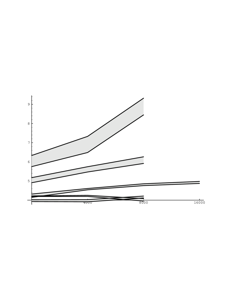
Figure 2: $D_{h}(N,\kappa)$ shown as a function of $N$ for (from top to bottom) $\beta=-\frac{1}{2}\log\kappa=0.14,0.15$, ($N=2K,4K$ and $8K$), $\beta^{*}\approx 0.1603$ ($N=2K,4K,8K$ and $16K$) and $\beta=0.17,0.18$ ($N=2K,4K$ and $8K$).

We see that for $\kappa>\kappa^{*}$ the value of $D_{h}(N,\kappa)$ is consistent with $d_{h}(s)=4$, which is the value for pure gravity ($\kappa\to\infty$). For $\kappa<\kappa^{*}$ the functions $D_{h}(N,\kappa)$ grow with $N$ at least logarithmically, which suggests that $D_{h}(N,\kappa)\to\infty$ for $N\to\infty$ for these values of $\kappa$. Exactly at the critical point $\kappa=\kappa^{*}$ we see a different behavior of $D_{h}(N,\kappa)$, consistent with $D_{h}(N,\kappa^{*})\to 6$ for $N\to\infty$. It is also clear from the slow rise of $D_{h}(N,\kappa^{*})$ that it will require much larger values of $N$ if one wants to obtain a high precision measurement of $\lim_{N\to\infty}D_{h}(N,\kappa^{*})$.

5 Discussion

For the Ising model we have verified that the two-point function defined as a function of the loop gas “time” $t_{s}$ indeed scales with a $d_{h}(s)\approx 6$, i.e. in agreement with (2). On the other hand the use of geodesic distance yields $d_{h}(g)\approx 4$. The results using geodesic distance are in perfect agreement with (1) for $c=-2$. However, for the Ising model coupled to two-dimensional quantum gravity the result $d_{h}(g)\approx 4$ are only marginally in agreement with the prediction $d_{h}=4.2...$ by (1). But certainly (2) is ruled out, when geodesic distance is used. The same conclusion was reached for $c=-2$ coupled to two-dimensional quantum gravity [16, 17].

While the loop gas time $t_{s}$ lacks any obvious geometric interpretation except for $c=0$, where it coincides with the ordinary geodesic distance, it is nevertheless the scaling governed by the dimensionality of $t_{s}$ which appears in the simplest way in matrix model calculations. Further, it is for this choice of “time” variable that it is simplest to develop a string field theory and a transfer matrix formalism. It follows from the transfer matrix formalism that the two-point function for fixed cosmological constant will decay exponentially in $t_{s}$ [9]. By an inverse Laplace transformation this implies the following large $t_{s}$ behavior for fixed space-time volume $N$:

$$n_{N}(s,t_{s})\sim\exp\left\{-\left(\frac{t_{s}}{N^{1/d_{h}(s)}}\right)^{\frac{d_{h}(s)}{d_{h}(s)-1}}\right\}.$$ (29)

¿From dimensional arguments it is tempting to relate $t_{s}$ and $t_{g}$ as follows

$$t_{s}^{d_{h}(s)}\sim t_{g}^{d_{h}(g)}..$$ (30)

This suggests that the long distance behavior of $n_{N}(g,t_{g})$ should be

$$n_{N}(g,t_{g})\sim\exp\left\{-\left(\frac{t_{g}^{\frac{d_{h}(g)}{d_{h}(s)}}}{N^{1/d_{h}(s)}}\right)^{\frac{d_{h}(s)}{d_{h}(s)-1}}\right\}.$$ (31)

This prediction can be tested numerically by a study of the tail of the distribution $n_{N}(g,t_{g})$. For $c=-2$ we have a power of $t_{g}^{3.56}$ (compared to a naive power $t_{g}^{1.39}$, assuming exponential decay of the two-point function for fixed cosmological constant, using geodesic distance), while for $c=1/2$ the power is $t_{g}^{4/5}$ (compared to $t_{g}^{4/3}$). These predictions seem not to be satisfied numerically and it is unlikely that there is a simple relation like (30) between $t_{s}$ and $t_{g}$.

References

- [1] N. Kawamoto, Y. Saeki and Y. Watabiki, unpublished; Y. Watabiki, Prog. Theor. Phys. Suppl. 114 (1993) 1, N. Kawamoto, Fractal Structure of Quantum Gravity in two Dimensions in Proceedings of the 7’th Nishinomiya-Yukawa Memorial Symposium Nov. 1992, Quantum Gravity, eds. K. Kikkawa and M. Ninomiya (World Scientific)
- [2] N. Ishibashi and H. Kawai, Phys. Lett. B322 (1994) 67, Phys. Lett. B352 (1995) 75
- [3] E. Domany, D. Mukamel, B. Nienhuis and A. Schwimmer, Nucl. Phys. B190 (1981) 279
- [4] B. Nienhuis, Phys. Rev. Lett. 49 (1982) 1062
- [5] VI.S. Dotsentko and V.A. Fateev, Nucl. Phys. B240 (1984) 312
- [6] I. Kostov, Mod. Phys. Lett. A4 (1989) 217
- [7] B. Duplantier and I. Kostov, Phys. Rev. Lett. 61 (1988) 1433
- [8] Y. Watabiki, Nucl. Phys. B441 (1995) 119
- [9] J. Ambjørn, C. Kristjansen and Y. Watabiki, Nucl. Phys. B504 (1997) 555.
- [10] B. Eynard and C. Kristjansen, Nucl. Phys. B455 (1995) 577.
- [11] S. Catterall, G. Thorleifsson, M. Bowick and V. John, Phys. Lett. B354 (1995) 58.
- [12] J. Ambjørn, J. Jurkiewicz and Y. Watabiki, Nucl. Phys. B454 (1995) 313.
- [13] J. Ambjørn and K.N. Anagnostopoulos, Nucl. Phys. B497 (1997) 445.
- [14] N.D. Hari Dass, B.E. Hanlon, T. Yukawa, Phys. Lett. B368 (1996) 556.
- [15] M.J. Bowick, S.M. Catterall and G. Thorleifsson, Phys. Lett. B391 (1997) 305
- [16] J. Ambjørn, K.N. Anagnostopoulos, T. Ichihara, L. Jensen, N. Kawamoto, Y. Watabiki and K. Yotsuji, Phys. Lett. B397 (1997) 117.
- [17] J. Ambjørn, K.N. Anagnostopoulos, T. Ichihara, L. Jensen, N. Kawamoto, Y. Watabiki and K. Yotsuji, The quantum space time of gravity, hep-lat/9706009, to appear in Nucl.Phys. B.
- [18] D. Boulatov and V.A. Kazakov, Phys. Lett. 186B (1987) 379.