1 Introduction

Traditionally, the participants of the “Ahrenshoop International Symposium on the Theory of Elementary Particles” form two nearly disjoint subsets, consisting of string theorists and lattice gauge theorists. So, for a plenary speaker the question arises: is it possible to give a talk which addresses both of these species? I don’t have an answer, but this contribution is meant as an attempt.

Considering the basic theoretical objects which are being studied, there is no apparent relation. The geometrical objects of string theory are world-sheets of open or closed strings. We shall not speak about the additional internal degrees of freedom here. A parameterized world-sheet is described by functions $x^{\mu}(\sigma,\tau)$. In lattice gauge theory, on the other hand, the basic objects are group valued variables $U(x,\mu)$ associated with the links $(x,\mu)$ of a space-time lattice. That looks very different.

Let us consider bosonic string theory in $d$ dimensional space-time a little bit closer. The Nambu-Goto action of a world sheet, parameterized by $x^{\mu}(\sigma,\tau)$, with $\mu$ running from 1 to $d$, is

$$S=\alpha\cdot\mbox{Area}=\alpha\int\!\!d\sigma d\tau\sqrt{g}\,,$$ (1)

where

$$g=\det\left(\frac{\partial x_{\mu}}{\partial\xi_{\alpha}}\frac{\partial x^{\mu}}{\partial\xi_{\beta}}\right),\hskip 28.45274pt\xi_{\alpha}=\sigma,\tau.$$ (2)

Most people would start from the Polyakov action [1] nowadays, but let us stick to the Nambu-Goto action for the time being.

To quantize string theory basically means to give meaning to functional integrals of the type

$$Z=\int\!\!D[x^{\mu}(\sigma,\tau)]\ e^{-S}\,.$$ (3)

As is known since long there are obstacles to naive quantization for any dimension $d$. After employing reparametrization invariance to fix the so-called conformal gauge, the remaining conformal symmetry is generated by operators $L_{n}$, which obey the Virasoro algebra

$$[L_{n},L_{m}]=(n-m)L_{n+m}+\frac{d-26}{12}(m^{3}-m)\delta_{n+m,0}\,,$$ (4)

where the ghost contribution to the $L_{n}$’s is included. Consistent straightforward quantization requires the central extension to vanish. Therefore only

$$d=26$$ (5)

is allowed.

Now let us turn to lattice gauge theory. The link variables $U(x,\mu)$ represent the gauge field $A_{\mu}(x)$ in the sense of elementary parallel transporters on the lattice:

$$U(x,\mu)\simeq e^{-aA_{\mu}(x)}\in{\rm SU}(N)\,,$$ (6)

where $a$ is the lattice constant. The simplest action for a lattice gauge field is the Wilson action

$$S=-\frac{\beta}{N}\sum_{p}{\rm Re\,Tr}\,U(p)\,,$$ (7)

where $p$ are the elementary plaquettes on the lattice, $U(p)$ is the ordered product of the four link variables belonging to the boundary of plaquette $p$, and $\beta$ is inversely proportional to the coupling constant squared. The basic functional integral is of the type

$$Z=\int\!\!D[U(x,\mu)]\,e^{-S}\,.$$ (8)

One method to evaluate such integrals approximatively is the strong coupling expansion, i.e. an expansion in powers of $\beta$, analogous to high temperature expansions in statistical mechanics. For example, the strong coupling expansion for Wilson loops leads to diagrams, which are (more or less) surfaces on the lattice bounded by the loop. These surfaces look like world-sheets of strings. Indeed, it turns out that the strong coupling expansion leads to confinement of static quarks, and the above-mentioned surfaces are related to confining strings between colour sources [2, 3].

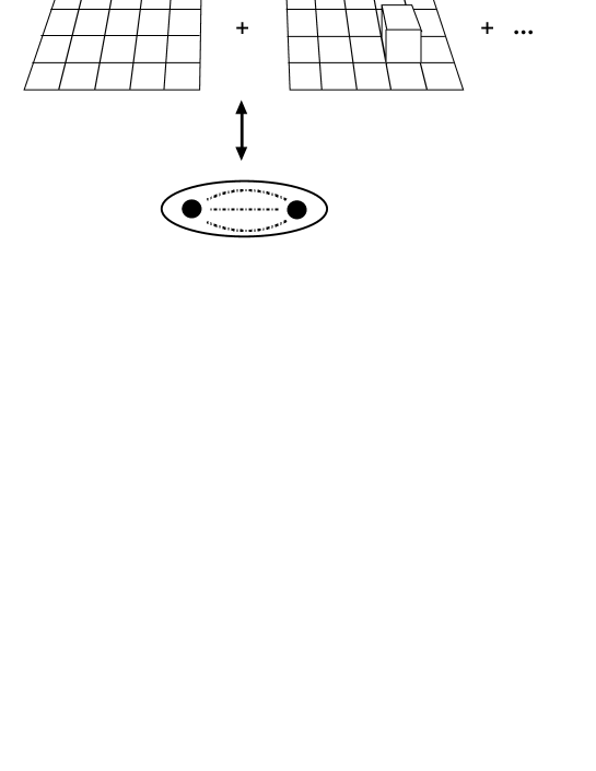
Figure 1: Strong coupling diagrams for a Wilson loop and the confining string

So there appears to be some relation between lattice gauge theory and strings. Can this relation be made more precise? In particular, is it possible to describe lattice gauge theory in terms of an effective string theory? Many attempts have been made in this direction, e.g. by Nielsen and Olesen, ’t Hooft, Nambu, Gervais and Neveu, Polyakov, Migdal and others [4]. It appears to be difficult to obtain concrete results.

As mentioned above, strings appear in the strong coupling expansion. It is, however, difficult to reformulate lattice gauge on the basis of the strong coupling expansion as a theory of strings. The main problem comes from the nontrivial weights of the diagrams.

Another point, where strings appear in lattice gauge theory, is the $1/N$-expansion [5], but it is difficult to obtain a string formulation for finite $N$ from that.

My impression is that the question of an effective string theory for gauge fields is still open. Let us therefore turn to simpler field theoretic models and look for strings in them. In particular, let us consider scalar fields. The simplest model with a scalar field is the Ising model. Its field $s(x)$ is associated with the points of a lattice and only assumes values $s(x)=\pm 1$, representing spins pointing up or down. The action is given by

$$S=-\kappa\sum_{<xy>}s(x)s(y)\,,$$ (9)

where $<xy>$ is a link between nearest neighbour points $x$ and $y$ on the lattice.

In the same universality class is $\phi^{4}$-theory. In the phase with broken symmetry the action can be written as

$$S=\int\!\!d^{d}x\left\{\frac{1}{2}(\partial_{\mu}\phi)^{2}+\frac{g}{4!}(\phi^{2}-v^{2})^{2}\right\}\,.$$ (10)

The minima of the double well potential are located at $\phi=\pm v$.

In the Ising model at large $\kappa$ (“low temperatures”), as well as in $\phi^{4}$-theory in the broken symmetric phase interfaces appear. They are $(d-1)$-dimensional surfaces separating regions with opposite values of the field. In the Ising model they are domain walls between regions with $s(x)=+1$ and $s(x)=-1$. For large enough $\kappa$ fluctuations are small and these interfaces are rather well defined objects. On a finite rectangular lattice with appropriate boundary conditions nearly flat interfaces can be prepared. Similarly, in the $\phi^{4}$-model interfaces separate regions with $\phi(x)\approx+v$ from those with $\phi(x)\approx-v$.

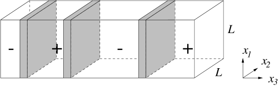
Figure 2: Interfaces in a finite Ising-like system

The interfaces of scalar field theory are string-like, i.e. two-dimensional, only for $d=3$, whereas the strings of lattice gauge theory are always two-dimensional. In $d=3$, where we have both types of “strings”, there is an interesting additional relation between them.

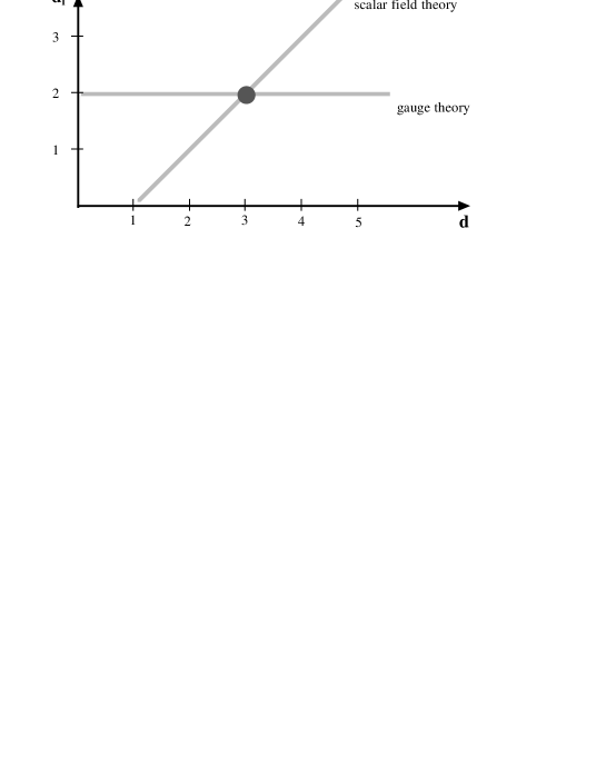
Figure 3: Dimensionality $d_{I}$ of surfaces in $d$ dimensions

This is duality, which can be made quite explicit for models with an abelian symmetry group. An abelian model, whose fields are p-forms and whose interaction terms are defined on $({\rm p}+1)$-cells, is mapped by duality onto an equivalent model of $(d-{\rm p}-2)$-forms and interactions on $(d-{\rm p}-1)$-cells. For $d=3$ duality maps the Ising model (p=0) at low temperatures onto the $Z_{2}$ gauge theory at high temperatures and vice versa. Therefore the Ising string in 3 dimensions is really the same as the $Z_{2}$ gauge theory string.

In the following we shall concentrate on the three-dimensional situation more closely.

2 Interfaces in $d=3$

There are many systems of statistical mechanics in three dimensions for which interfaces play an interesting role. These include

• liquid gas coexistence

• binary liquid mixtures

• anisotropic ferromagnetism

• ferroelectrics

• superconductors

• crystal growth.

Near a critical point ($T\approx T_{c}$) of such a system one observes universal behaviour of certain quantities related to interfaces. Consider the interface tension $\tau$ or the reduced interface tension $\sigma=\tau/kT$, where $k$ is Boltzmann’s constant. It is positive for $T<T_{c}$, but vanishes according to

$$\sigma\sim\sigma_{0}\left|\frac{T-T_{c}}{T_{c}}\right|^{\mu}$$ (11)

as the temperature $T$ approaches $T_{c}$. The value of the critical exponent is approximately $\mu\approx 1.26$ and appears to be universal. On the other hand, the amplitude $\sigma_{0}$ is not universal.

The critical law for the correlation length $\xi$, which diverges at the critical point, is

$$\xi\sim\xi_{0}\left|\frac{T-T_{c}}{T_{c}}\right|^{-\nu}\,.$$ (12)

Widom’s scaling law [6] relates the indices $\mu$ and $\nu$. In $d=3$ it reads

$$\mu=2\nu\,.$$ (13)

Consequently the product $\sigma\xi^{2}$ approaches a finite value at the critical point:

$$\sigma\xi^{2}\longrightarrow\sigma_{0}\xi_{0}^{2}\doteq R_{-}\,.$$ (14)

The number $R_{-}$ appears to be universal, too. It is a so-called universal amplitude product. In the past it has been studied experimentally for various systems, by means of Monte Carlo calculations, and by field theoretic methods. Other quantities, which have been investigated in connection with interfaces, are the interface width, the interface profile, the interface stiffness etc.. Closely related to $R_{-}$ is

$$R_{+}=\sigma_{0}(\xi_{0}^{+})^{2}=R_{-}\left(\frac{\xi_{0}^{+}}{\xi_{0}^{-}}\right)^{2}\,,$$ (15)

where $\xi_{0}^{+}$ is the correlation length amplitude of the high temperature phase (which is easier accessible experimentally), and $\xi_{0}^{-}$ the one of the low temperature phase.

Why should one study $R_{-}$ or $R_{+}$? Early results from the $\epsilon$-expansion [7] and from Monte-Carlo calculations [8] were in strong conflict with experimental numbers $R_{+}=0.38(2)$ (for a brief summary of the history and relevant references see [9]). Therefore the question of universality for these interface-related quantities arose. Furthermore it became desirable to learn about the status of the theoretical predictions.

So, let us turn to the theoretical calculation of the interface tension.

3 Description of interfaces by field theory

The critical phenomena of systems in the universality class of the three-dimensional Ising model, like those mentioned in the previous section, can be calculated in the framework of massive $\phi^{4}$-theory. The scalar field $\phi(x)$ represents the order parameter. For example in the case of a liquid mixture this would be the difference of densities of the two liquids. The action for the scalar field is given in Eq. (10). In order to study a planar interface we consider the theory in a rectangular box with quadratic cross-section $L^{2}$ in the $x_{1}-x_{2}$-plane and antiperiodic boundary conditions in the $x_{3}$-direction. Alternatively, one might choose

$$\phi(x)\longrightarrow\left\{\begin{array}[]{l}+v,\hskip 11.38109pt\mbox{as}\ x_{3}\rightarrow\infty\\ -v,\hskip 11.38109pt\mbox{as}\ x_{3}\rightarrow-\infty\,.\end{array}\right.$$ (16)

A classical solution of the field equations is given by the kink

$$\phi_{c}=\sqrt{\frac{3m^{2}}{g}}\tanh\frac{m}{2}(x_{3}-a)\,,$$ (17)

centered at $x_{3}=a$, where $m^{2}=gv^{2}/3$.

Figure 4: The kink as an interface between two phases

Its classical action is

$$S_{c}=2\frac{m^{3}}{g}L^{2}\,.$$ (18)

Thus the saddle point approximation to the functional integral with the boundary conditions specified above,

$$Z_{+-}=\int_{\pm}D\phi\ e^{-S}\,,$$ (19)

is given by

$$Z_{+-}\approx e^{-S_{c}}\,.$$ (20)

Because $Z_{+-}$ is the partition function of a system with an interface, it should depend on $L$ like

$$Z_{+-}\sim e^{-\sigma L^{2}}\,.$$ (21)

We can read off the interface tension in the saddle point approximation

$$\sigma\approx 2\frac{m^{3}}{g}\,,$$ (22)

and for the product of interest we obtain

$$\sigma\xi^{2}=\frac{\sigma}{m^{2}}\approx 2\frac{m}{g}\,.$$ (23)

Introducing the dimensionless coupling constant

$$u\equiv\frac{g}{m}\,,$$ (24)

we write our tree level result as

$$\frac{\sigma}{m^{2}}\approx\frac{2}{u}\,.$$ (25)

Now let us take into account fluctuations

$$\phi(x)=\phi_{c}(x)+\eta(x)$$ (26)

around the classical solution. The action

$$S=S_{c}+\frac{1}{2}\int\!\!d^{3}x\,\eta(x)M\eta(x)+O(\eta^{3})$$ (27)

contains the fluctuation operator

$$M=-\partial_{\mu}\partial^{\mu}+m^{2}-\frac{3}{2}m^{2}\cosh^{-2}(\frac{m}{2}x_{3})\,.$$ (28)

For the case of periodic boundary conditions, where an interface need not be present, the partition function is denoted $Z_{++}$, and $M$ is replaced by the Helmholtz operator

$$M_{0}=-\partial_{\mu}\partial^{\mu}+m^{2}\,.$$ (29)

The relevant ratio of partition functions can then expressed as

(31)

where the meaning of the graphs can be found in [10]. To evaluate this expression, first of all renormalization has to be carried out in the usual way. Moreover, the contribution of multi-kink configurations has been taken into account, but I refuse to reveal any details here.

Luckily, in the one-loop approximation the determinants can be calculated exactly [11] and one obtains

$$\frac{Z_{+-}}{Z_{++}}=Ce^{-\sigma L^{2}}\,,$$ (32)

with

$$\frac{\sigma}{m^{2}}=\frac{2}{u_{R}}\left(1+\sigma_{1}\frac{u_{R}}{4\pi}+\ldots\right)$$ (33)

and exact expressions for the constants $C$ and $\sigma_{1}$. The quantities $m$ and $u_{R}$ are the renormalized mass and coupling now.

Believe it or not, it has been possible to evaluate the two-loop contribution to the ratio $\sigma/m^{2}$, too [10]. Written in the form

$$\sigma_{2}\left(\frac{u_{R}}{4\pi}\right)^{2}$$ (34)

the coefficient $\sigma_{2}=-0.0076(8)$ turns out to be rather small. In order to obtain the desired universal ratio we have to evaluate the function

$$\frac{\sigma}{m^{2}}\equiv R_{-}(u_{R})$$ (35)

at the fixed point value $u_{R}=u_{R}^{*}$. The most recent value $u_{R}^{*}=14.3(1)$ from Monte Carlo calculations [12] is consistent with an estimate of 14.2(2) from three-dimensional field theory [13]. At this value of the coupling the one-loop contribution is 24% and the two-loop contribution roughly 1% of the tree-level term. The final result from field theory for the amplitude product is

$$R_{-}=0.1065(9)\,.$$ (36)

It compares well with the recent Monte Carlo result $R_{-}=0.1040(8)$ by Hasenbusch and Pinn [14]. The corresponding numbers for $R_{+}$, using theoretical values for $\xi_{0}^{+}/\xi_{0}^{-}$, lie in the range from 0.40(1) to 0.42(1) and are compatible with the recent experimental result $R_{+}=0.41(4)$ [15], which is higher than the earlier average of 0.37(3).

4 Effective string description

Field theory describes fluctuating interfaces, as we have seen. The relevant partition function is analogous to a functional integral over fluctuating string world-sheets, Eq. (3). A proposal to describe the dynamics of fluctuating interfaces in terms of an effective string model is the “capillary wave model” or “drumhead model” [16]. The interface is considered to be a surface without overhangs, which can be described by a height function $x_{3}=h(x_{1},x_{2})$.

Figure 5: Smooth surface in the drumhead model

The action is, as in the Nambu-Goto case, given by the area:

$$S=\tilde{\sigma}\int_{0}^{L_{1}}\!\!dx_{1}\int_{0}^{L_{2}}\!\!dx_{2}\sqrt{1+\left(\frac{\partial h}{\partial x_{1}}\right)^{2}+\left(\frac{\partial h}{\partial x_{2}}\right)^{2}}\,.$$ (37)

Expanding in powers of $h$ we get

$$S = \tilde{\sigma}L_{1}L_{2}+\frac{\tilde{\sigma}}{2}\int\!\!dx_{1}\int\!\!dx_{2}\left[\left(\frac{\partial h}{\partial x_{1}}\right)^{2}+\left(\frac{\partial h}{\partial x_{2}}\right)^{2}\right]$$ (38)

$$-\frac{\tilde{\sigma}}{8}\int\!\!dx_{1}\int\!\!dx_{2}\left[\left(\frac{\partial h}{\partial x_{1}}\right)^{2}+\left(\frac{\partial h}{\partial x_{2}}\right)^{2}\right]^{2}+\cdots$$

The second term, the Gaussian action $S_{G}$, is quadratic in the field $h(x_{1},x_{2})$ and describes a massless scalar field in two dimensions. The expansion of the action above leads to an expansion of the partition function which is organized in powers of $1/\tilde{\sigma}L_{1}L_{2}$:

$$Z_{+-}=e^{-\tilde{\sigma}L_{1}L_{2}}\ Z_{1}\cdot Z_{2}\cdot\ldots$$ (39)

where the one-loop term

$$Z_{1}=\int\!\!Dh\,e^{-S_{G}}=(\det\Delta_{(2)})^{-1/2}$$ (40)

can be expressed in terms of the determinant of the two-dimensional Laplace operator with appropriate boundary conditions. This is a well known object in 2d conformal invariant field theory with central charge $c=1$ on a torus [17], and has been calculated explicitly:

$$Z_{1}=\frac{1}{\sqrt{-i\tau}}\left|\frac{\eta(\tau)}{\eta(i)}\right|^{-2}\cdot\mbox{const.}\,,$$ (41)

where

$$\eta(\tau)=q^{1/24}\prod_{n=1}^{\infty}(1-q^{n})\,,\hskip 14.22636ptq=e^{2\pi i\tau}$$ (42)

is Dedekind’s eta-function, and the parameter $\tau$ is given by the aspect ratio

$$\tau=i\frac{L_{1}}{L_{2}}\,.$$ (43)

This opens the possibility to test the capillary wave model by studying the dependence of $Z_{1}$ on $L_{1}/L_{2}$. Comparing two partition functions with equal area, $L^{2}=L_{1}L_{2}$, the leading term cancels out and one has

$$\frac{Z_{+-}(L_{1},L_{2})}{Z_{+-}(L,L)}=\sqrt{\frac{L_{2}}{L_{1}}}\left|\frac{\eta(iL_{1}/L_{2})}{\eta(i)}\right|^{-2}\,.$$ (44)

A comparison of this formula with Monte Carlo results for the $d=3$ Ising model shows very good agreement, supporting the capillary wave model [18].

The capillary wave model also predicts the roughening phenomenon [16]. The width $w$ of an interface of size $L\times L$, given by

$$w^{2}=\frac{1}{L^{2}}\int\!\!dx_{1}dx_{2}\ \langle(h(x_{1},x_{2})-\langle h\rangle)^{2}\rangle\,,$$ (45)

can be calculated in the Gaussian capillary wave model [19, 20]. For large $L$ it diverges like

$$w^{2}=\frac{1}{2\pi\sigma}\log\frac{L}{R_{0}}\,,$$ (46)

with some cutoff length $R_{0}$. This behaviour indicates the dominance of longwave fluctuations of the interface.

The Gaussian approximation, considered so far, is not specific to the capillary wave model. In fact, it is an infrared fixed point for a whole class of effective models. In order to test the capillary wave model one should go beyond the Gaussian approximation. This has been done in [21] (see also [22]). They have evaluated the two-loop contribution $Z_{2}$ to the partition function and get

$$Z_{2} = 1+\frac{\tilde{\sigma}}{8}\int\!\!dx_{1}\int\!\!dx_{2}\ \langle((\nabla h)^{2})^{2}\rangle_{G}$$ (47)

$$= 1+\frac{1}{4\sigma L^{2}}$$

for $L_{1}=L_{2}=L$. Included is a renormalization of the interface tension $\sigma$. This term has been nicely confirmed by Monte Carlo calculations [21].

At this point one might wonder whether it is possible to derive the string description, i.e. the capillary wave model, directly from $\phi^{4}$-theory in three dimensions. In the Gaussian approximation this can indeed be done, see [23]. The fluctuation operator $M$, Eq. (28), decomposes into the two-dimensional Laplacean $\Delta_{(2)}$ and a Schrödinger operator $Q$: $M=-\Delta_{(2)}+Q$. The operator $Q$ has two discrete eigenvalues, 0 and $3m^{2}/4$, and a continuous spectrum. The zero-mode is associated with translations of the interface along $x_{3}$. Consequently, the determinant of $M$ contains $\det\Delta_{(2)}$ as a factor. But this is just the contribution of a two-dimensional free massless scalar field, and is identical to the Gaussian capillary wave model. The remaining factor belongs to massive modes on the interface and does not dominate the long-wavelength behaviour. It contributes to the renormalization of $\sigma$.

To derive the string model from $\phi^{4}$ theory beyond the Gaussian approximation of interface fluctuations is more difficult. First of all, for a given field $\phi(x)$ the interface variables $h(x_{1},x_{2})=F[\phi(x)]$ have to be defined suitably, at least for fields not too far away from the kink solution $\phi_{c}$. Formally one would then write

$$\int\!\!D[\phi(x)]\ e^{-S}\equiv\int\!\!D[h(\xi)]\ e^{-S_{h}}$$ (48)

with

$$e^{-S_{h}}=\int\!\!D[\phi(x)]\ e^{-S}\delta[h(\xi)-F[\phi(x)]\,.$$ (49)

This approach has been studied e.g. in [24, 25]. In the low temperature limit, $T\rightarrow 0$, the interface (or string) action $S_{h}$ indeed approaches the Nambu-Goto action

$$S_{h}=\sigma\cdot\mbox{Area}+\mbox{corrections}\,.$$ (50)

This is, however, far away from the critical point.

5 Questions

Many questions concerning the relation of critical interfaces to strings are still open. Let us consider fluctuations. Near the critical point the fluctuations of the interface are strong. In the field theoretic approach this means that a typical field $\phi$ is by no means similar to the classical solution $\phi_{c}$. Why then, does the semiclassical expansion work so well?

We can interpret this effect as a result of renormalization. Fluctuations on short scales produce ultraviolet divergencies, which lead to the renormalization of the mass $m$ and the interface tension $\sigma$. In the renormalized propagator in a kink background the UV-fluctuations are summed up effectively. In terms of renormalized quantities we can thus expect a smoother behaviour. So it is the usual picture of renormalization, which is at work.

On the side of the string description the same question arises. Near the critical point the interface is far from smooth. Overhangs, bubbles and handles appear. Why does the capillary wave model work?

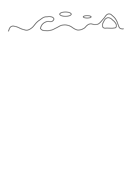
Figure 6: Overhangs, bubbles and handles

Attempts to answer this question have been made in [26]. The analogue of renormalization is claimed to be a “condensation of handles”. Near each point of the interface thin tubes can be attached, which represent overhangs or handles. They yield a renormalization factor proportional to the area, which in turn can be absorbed into the renormalization of the tension $\sigma$. The average size of a handle is expected to be microscopic and independent of the large scale geometry of the interface, so that these condensed handles do not influence the long-wavelength behaviour.

Another question concerns the conformal anomaly. The bosonic string can be quantized consistently without Liouville modes only in 26 dimensions. Why does the effective string model work in 3 dimensions?

A more careful treatment of the transformation from field variables to string variables would take into account the arising Jacobian $J$:

$$e^{-S_{h}}=\int\!\!D[\phi(x)]\ e^{-S}J[h(\xi)]\,\delta[h(\xi)-F[\phi(x)]]\,.$$ (51)

A calculation of $J$ in the framework of a four-dimensional abelian Higgs-model [27] gave

$$J=\mbox{const.}\exp\left\{\int\!\!d^{2}\xi\frac{22}{96\pi}(\partial_{a}\log\sqrt{g})^{2}+\ldots\right\}.$$ (52)

This term contributes to the Virasoro generators $L_{n}$, and their algebra reads

$$[L_{n},L_{m}]=(n-m)L_{n+m}+\frac{d-26+22}{12}(m^{3}-m)\delta_{n+m,0}\,.$$ (53)

The anomaly term now vanishes in $d=4$ dimensions, as desired. The string action is given by

$$S_{h}=\int\!\!d^{2}\xi\left\{\sigma\sqrt{g}-\frac{11}{48\pi}(\partial_{a}\log\sqrt{g})^{2}-\beta\sqrt{g}(\partial_{a}t_{\mu\nu})^{2}+\ldots\right\}\,,$$ (54)

where $t_{\mu\nu}$ is the extrinsic curvature. The second piece, the Liouville term, has been first proposed in [28].

Because the Jacobian $J$ is of a pure geometric nature, the same effect is expected to take place in three-dimensional $\phi^{4}$-theory.

To summarize, there are interesting relations between string theory and fluctuating interfaces in critical statistical systems, and there are several open points, which deserve further study.

References

- [1] A.M. Polyakov, Phys. Lett. B 103 (1981) 207
- [2] K.G. Wilson, Phys. Rev. D 10 (1974) 2445
- [3] J. Kogut, L. Susskind, Phys. Rev. D 11 (1975) 395
- [4] H.B. Nielsen, P. Olesen, Nucl. Phys. B 61 (1973) 45 G. ’t Hooft, Nucl. Phys. B 72 (1974) 461 Y. Nambu, Phys. Lett. B 80 (1979) 372 J.L. Gervais, A. Neveu, Nucl. Phys. B 163 (1980) 189 A.M. Polyakov, Nucl. Phys. B 164 (1980) 179 A.A. Migdal, Nucl. Phys. B 189 (1981) 253
- [5] B. de Wit, G. ’t Hooft, Phys. Lett. B 69 (1977) 61
- [6] B. Widom, J. Chem. Phys. 43 (1965) 3892
- [7] E. Brézin, S. Feng, Phys. Rev. B 29 (1984) 472
- [8] K. Binder, Phys. Rev. A 25 (1982) 1699
- [9] G. Münster, Int. J. Mod. Phys. C 3 (1992) 879
- [10] P. Hoppe, G. Münster, Phys. Lett. A (1998), in press
- [11] G. Münster, Nucl. Phys. B 340 (1990) 559
- [12] M. Caselle, M. Hasenbusch, J. Phys. A 30 (1997) 4963
- [13] C. Gutsfeld, J. Küster, G. Münster, Nucl. Phys. B 479 (1996) 654
- [14] M. Hasenbusch, K. Pinn, Physica A 245 (1997) 366
- [15] T. Mainzer, D. Woermann, Physica A 225 (1996) 312
- [16] F.P. Buff, R.A. Lovett, F.H. Stillinger Jr., Phys. Rev. Lett. 15 (1965) 621
- [17] C. Itzykson, J.-B. Zuber, Nucl. Phys. B 275 (1986) 580
- [18] M. Caselle, F. Gliozzi, S. Vinti, Phys. Lett. B 302 (1993) 74
- [19] M. Lüscher, G. Münster, P. Weisz, Nucl. Phys. B 180 (1981) 1
- [20] M. Hasenbusch, K. Pinn, Physica A 192 (1993) 342
- [21] M. Caselle et al., Nucl. Phys. B 432 (1994) 590
- [22] K. Dietz, T. Filk, Phys. Rev. D 27 (1983) 2944
- [23] P. Provero, S. Vinti, Nucl. Phys. B 441 (1995) 562
- [24] H.W. Diehl, D.M. Kroll, H. Wagner, Z. Phys. B 36 (1980) 329
- [25] R.K.P. Zia, Nucl. Phys. B 251 (1985) 676
- [26] M. Ademollo et al., Nucl. Phys. B 94 (1975) 221 M. Caselle, F. Gliozzi, S. Vinti, Nucl. Phys. (Proc. Suppl.) B 34 (1994) 726 V. Dotsenko et al., Phys. Rev. Lett. 71 (1993) 811
- [27] E.T. Akhmedov, M.N. Chernodub, M.I. Polikarpov, M.A. Zubkov, Phys. Rev. D 53 (1996) 2087
- [28] J. Polchinski, A. Strominger, Phys. Rev. Lett. 67 (1991) 1681