Lectures on D-branes, Gauge Theory and M(atrices)

Abstract

These notes give a pedagogical introduction to D-branes and Matrix theory. The development of the material is based on super Yang-Mills theory, which is the low-energy field theory describing multiple D-branes. The main goal of these notes is to describe physical properties of D-branes in the language of Yang-Mills theory, without recourse to string theory methods. This approach is motivated by the philosophy of Matrix theory, which asserts that all the physics of light-front M-theory can be described by an appropriate super Yang-Mills theory.

Table of Contents
1. Introduction
2. D-branes and Super Yang-Mills Theory
3. D-branes and Duality (T-duality and S-duality in D-brane SYM theory)
4. Branes and Bundles (Constructing $(p\pm 2k)$-branes from $p$-branes)
5. D-brane Interactions
6. M(atrix) theory: The Conjecture
7. Matrix theory: Symmetries, Objects and Interactions
8. Matrix theory: Further Developments
9. Conclusions

1 Introduction

1.1 Orientation

In the last several years there has been a revolution in string theory. There are two major developments responsible for this revolution.

i. It has been found that all five string theories, as well as 11-dimensional supergravity, are related by duality symmetries and seem to be aspects of one underlying theory whose fundamental principles have not yet been elucidated.

ii. String theories contain Dirichlet $p$-branes, also known as “D-branes”. These objects have been shown to play a fundamental role in nonperturbative string theory.

Dirichlet $p$-branes are dynamical objects which are extended in $p$ spatial dimensions. Their low-energy physics can be described by supersymmetric gauge theory. The goal of these lectures is to describe the physical properties of D-branes which can be understood from this Yang-Mills theory description. There is a two-fold motivation for taking this point of view. At the superficial level, super Yang-Mills theory describes much of the interesting physics of D-branes, so it is a nice way of learning something about these objects without having to know any sophisticated string theory technology. At a deeper level, there is a growing body of evidence that super Yang-Mills theory contains far more information about string theory than one might reasonably expect. In fact, the recent Matrix theory conjecture [?] essentially states that the simplest possible super Yang-Mills theory with 16 supersymmetries, namely ${\cal N}=16$ super Yang-Mills theory in 0 + 1 dimensions, completely reproduces the physics of eleven-dimensional supergravity in light-front gauge.

The point of view taken in these lectures is that many interesting aspects of string theory can be derived from Yang-Mills theory. This is a theme which has been developed in a number of contexts in recent research. Conversely, one of the other major themes of recent developments in formal high-energy theory has been the idea that string theory can tell us remarkable things about low-energy field theories such as super Yang-Mills theory, particularly in a nonperturbative context. In these lectures we will not discuss any results of the latter variety; however, it is useful to keep in mind the two-way nature of the relationship between string theory and Yang-Mills theory.

The body of knowledge related to D-branes and Yang-Mills theory is by now quite enormous and is growing steadily. Due to limitations on time, space and the author’s knowledge there are many interesting developments which cannot be covered here. As always in an effort of this sort, the choice of topics covered largely reflects the prejudices of the author. An attempt has been made, however, to concentrate on a somewhat systematic development of those concepts which are useful in understanding recent progress in Matrix theory. For a comprehensive review of D-branes in string theory, the reader is referred to the reviews of Polchinski et al. [?, ?].

These lectures begin with a review of how the low-energy Yang-Mills description of D-branes arises in the context of string theory. After this introduction, we take super Yang-Mills theory as our starting point and we proceed to discuss a number of aspects of D-brane and string theory physics from this point of view. In the last lecture we use the technology developed in the first four lectures to discuss the recently developed Matrix theory.

1.2 D-branes from string theory

We now give a brief review of the manner in which D-branes appear in string theory. In particular, we give a heuristic description of how supersymmetric Yang-Mills theory arises as a low-energy description of parallel D-branes. The discussion here is rather abbreviated; the reader interested in further details is referred to the reviews of Polchinski et al. [?, ?] or to the original papers mentioned below.

Figure 1: D-branes (gray) are extended objects on which strings (black) can end

In string theory, Dirichlet $p$-branes are defined as $(p+1)$-dimensional hypersurfaces in space-time on which strings are allowed to end (see Figure 1). From the point of view of perturbative string theory, the positions of the D-branes are fixed, corresponding to a particular string theory background. The massless modes of the open strings connected to the D-branes can be associated with fluctuation modes of the D-branes themselves, however, so that in a full nonperturbative context the D-branes are expected to become dynamical $p$-dimensional membranes. This picture is analogous to the way in which, in a particular metric background for perturbative string theory, the quantized closed string has massless graviton modes which provide a mechanism for fluctuations in the metric itself.

The spectrum of low-energy fields in a given string background can be simply computed from the string world-sheet field theory [?]. Let us briefly review the analyses of the spectra for the string theories in which we will be interested. We consider two types of strings: open strings, with endpoints which are free to move independently, and closed strings, with no endpoints. A superstring theory is defined by a conformal field theory on the $(1+1)$-dimensional string world-sheet, with free bosonic fields $X^{\mu}$ corresponding to the position of the string in 10 space-time coordinates, and fermionic fields $\psi^{\mu}$ which are partners of the fields $X^{\mu}$ under supersymmetry. Just as for the classical string studied in beginning physics courses, the degrees of freedom on the open string correspond to standing wave modes of the fields; there are twice as many modes on the closed string, corresponding to right-moving and left-moving waves. The open string boundary conditions on the bosonic fields $X^{\mu}$ can be Neumann or Dirichlet for each field separately. When all boundary conditions are Neumann the string endpoints move freely in space. When $9-p$ of the fields have Dirichlet boundary conditions, the string endpoints are constrained to lie on a $p$-dimensional hypersurface which corresponds to a D-brane. Different boundary conditions can also be chosen for the fermion fields on the string. On the open string, boundary conditions corresponding to integer and half-integer modes are referred to as Ramond (R) and Neveu-Schwarz (NS) respectively. For the closed string, we can separately choose periodic or antiperiodic boundary conditions for the left- and right-moving fermions. These give rise to four distinct sectors for the closed string: NS-NS, R-R, NS-R and R-NS.

Straightforward quantization of either the open or closed superstring theory leads to several difficulties: the theory seems to contain a tachyon with $M^{2}<0$, and the theory is not supersymmetric from the point of view of ten-dimensional space-time. It turns out that both of these difficulties can be solved by projecting out half of the states of the theory. For the open string theory, there are two choices of how this GSO projection operation can be realized. These two projections are equivalent, however, so that there is a unique spectrum for the open superstring. For the closed string, on the other hand, one can either choose the same projection in the left and right sectors, or opposite projections. These two choices lead to the physically distinct IIA and IIB closed superstring theories, respectively.

From the point of view of 10D space-time, the massless fields arising from quantizing the string theory and incorporating the GSO projection can be characterized by their transformation properties under ${\rm spin}(8)$ (this is the covering group of the group $SO(8)$ which leaves a lightlike momentum vector invariant). We will now simply quote these results from [?]. For the open string, in the NS sector there is a vector field $A_{\mu}$, transforming under the $8_{v}$ representation of ${\rm spin}(8)$ and in the R sector there is a fermion $\psi$ in the $8_{s}$ representation. The massless fields for the IIA and IIB closed strings in the NS-NS and R-R sectors are given in the following table:

	NS-NS	R-R
IIA	$g_{\mu\nu},\phi,B_{\mu\nu}$	$A^{(1)}_{\mu},A^{(3)}_{\mu\nu\rho}$
IIB	$g_{\mu\nu},\phi,B_{\mu\nu}$	$A^{(0)},A^{(2)}_{\mu\nu},A^{(4)}_{\mu\nu\rho\sigma}$

The IIA and IIB strings have the same fields in the NS-NS sector, corresponding to the space-time metric $g_{\mu\nu}$, dilaton $\phi$ and antisymmetric tensor field $B_{\mu\nu}$. In addition, each closed string theory has a set of R-R fields. For the IIA theory there are 1-form and 3-form fields. For the IIB theory there is a second scalar field (the axion), a second 2-form field, and a 4-form field $A^{(4)}$ which is self-dual. The NS-NS and R-R fields all correspond to space-time bosonic fields. In both the IIA and IIB theories there are also fields in the NS-R and R-NS sectors corresponding to space-time fermionic fields.

Until recently, the role of the R-R fields in string theory was rather unclear. In one of the most important papers in the recent string revolution [?], however, it was pointed out by Polchinski that D-branes are charge carriers for these fields. Generally, a Dirichlet $p$-brane couples to the R-R $(p+1)$-form field through a term of the form

$$\mu_{p}\int_{\Sigma_{(p+1)}}A^{(p+1)}$$ (1)

where the integral is taken over the $(p+1)$-dimensional world-volume of the $p$-brane.

In type IIA theory there are Dirichlet $p$-branes with $p=0,2,4,6,8$ and in type IIB there can be Dirichlet $p$-branes with $p=-1,1,3,5,7,9$. The D-branes with $p>3$ couple to the duals of the R-R fields, and are thus magnetically charged under the corresponding R-R fields. For example, a Dirichlet 6-brane, with a 7-dimensional world-volume, couples to the 7-form whose 8-form field strength is the dual of the 2-form field strength of $A^{(1)}$. Thus, the Dirichlet 6-brane is magnetically charged under the R-R vector field in IIA theory. The story is slightly more complicated for the Dirichlet 8-brane and 9-brane [?]; however, 8-branes and 9-branes will not appear in these lectures in any significant way.

In addition to the Dirichlet $p$-branes which appear in type IIA and IIB string theory, there are also solitonic NS-NS 5-branes which appear in both theories, which are magnetically charged under the NS-NS two-form field $B_{\mu\nu}$. In the remainder of these notes $p$-branes which are not explicitly stated to be Dirichlet or NS-NS are understood to be Dirichlet $p$-branes; we will also sometimes use the notation D$p$-brane to denote a $p$-brane of a particular dimension.

It is interesting to see how the dynamical degrees of freedom of a D-brane arise from the massless string spectrum in a fixed D-brane background [?]. In the presence of a D-brane, the open string vector field $A_{\mu}$ decomposes into components parallel to and transverse to the D-brane world-volume. Because the endpoints of the strings are tied to the world-volume of the brane, we can interpret these massless fields in terms of a low-energy field theory on the D-brane world-volume. The $p+1$ parallel components of $A_{\mu}$ turn into a $U(1)$ gauge field $A_{\alpha}$ on the world-volume, while the remaining $9-p$ components appear as scalar fields $X^{a}$. The fields $X^{a}$ describe fluctuations of the D-brane world-volume in transverse directions. In general throughout these notes we will use $\mu,\nu,\ldots$ to denote 10D indices, $\alpha,\beta,\ldots$ to denote $(p+1)$-D indices on a D-brane world-volume, and $a,b,\ldots$ to denote $(9-d)$-D transverse indices.

One way to learn about the low-energy dynamics of a D-brane is to find the equations of motion for the D-brane which must be satisfied for the open string theory in the D-brane background to be conformally invariant. Such an analysis was carried out by Leigh [?]. He showed that in a purely bosonic theory, the equations of motion for a D-brane are precisely those of the action

$$S=-T_{p}\int d^{p+1}\xi\;e^{-\phi}\;\sqrt{-\det(G_{\alpha\beta}+B_{\alpha\beta}+2\pi\alpha^{\prime}F_{\alpha\beta})}$$ (2)

where $G$, $B$ and $\phi$ are the pullbacks of the 10D metric, antisymmetric tensor and dilaton to the D-brane world-volume, while $F$ is the field strength of the world-volume $U(1)$ gauge field $A_{\alpha}$. This action can be verified by a perturbative string calculation [?], which also gives a precise expression for the brane tension

$$\tau_{p}=\frac{T_{p}}{g}=\frac{1}{g\sqrt{\alpha^{\prime}}}\frac{1}{(2\pi\sqrt{\alpha^{\prime}})^{p}}$$ (3)

where $g=e^{\langle\phi\rangle}$ is the string coupling, equal to the exponential of the dilaton expectation value, and $\alpha^{\prime}$ is related to the string tension through

$$\frac{1}{2\pi\alpha^{\prime}}=T_{{\rm string}}.$$ (4)

The inverse string coupling appears because the leading string diagram which contributes to the action (2) is a disk diagram.

In the full supersymmetric string theory, the action (2) must be extended to a supersymmetric Born-Infeld type action. In addition, there are Chern-Simons type terms coupling the D-brane gauge field to the R-R fields, of which the leading term is the $\int A^{(p+1)}$ term discussed above; we will discuss these terms in more detail later in these notes.

If we make a number of simplifying assumptions, the form of the action (2) simplifies considerably. First, let us assume that the background ten-dimensional space-time is flat, so that $g_{\mu\nu}=\eta_{\mu\nu}$ (we use a metric with signature $-++\cdots++$). Further, let us assume that the D-brane is approximately flat and that we can identify the world-volume coordinates on the D-brane with $p+1$ of the ten-dimensional coordinates (the static gauge assumption). Then, the pullback of the metric to the D-brane world-volume becomes

$$G_{\alpha\beta}\approx\eta_{\alpha\beta}+\partial_{\alpha}X^{a}\partial_{\beta}X^{a}+{\cal O}\left((\partial X)^{4}\right)$$ (5)

If we make the further assumptions that $B_{\mu\mu}$ vanishes, and that $2\pi\alpha^{\prime}F_{\alpha\beta}$ and $\partial_{\alpha}X^{a}$ are small and of the same order, then we see that the low-energy D-brane world-volume action becomes

$$S=-\tau_{p}V_{p}-\frac{1}{4g_{{\rm YM}}^{2}}\int d^{p+1}\xi\left(F_{\alpha\beta}F^{\alpha\beta}+\frac{2}{(2\pi\alpha^{\prime})^{2}}\partial_{\alpha}X^{a}\partial^{\alpha}X^{a}\right)+{\cal O}(F^{4})$$ (6)

where $V_{p}$ is the $p$-brane world-volume and the coupling $g_{\rm YM}$ is given by

$$g_{\rm YM}^{2}=\frac{1}{4\pi^{2}\alpha^{\prime 2}\tau_{p}}=\frac{g}{\sqrt{\alpha^{\prime}}}(2\pi\sqrt{\alpha^{\prime}})^{p-2}$$ (7)

The second term in (6) is essentially just the action for a $U(1)$ gauge theory in $p+1$ dimensions with $9-p$ scalar fields. In fact, after including fermionic fields $\psi$ the low-energy action for a D-brane becomes precisely the supersymmetric $U(1)$ Yang-Mills theory in $p+1$ dimensions which arises from dimensional reduction of the $U(1)$ Yang-Mills theory in 10 dimensions with ${\cal N}=1$ supersymmetry. The action of this 10D theory is

$$S=\frac{1}{g_{\rm YM}^{2}}\int d^{10}\xi\;\left(-\frac{1}{4}F_{\mu\nu}F^{\mu\nu}+\frac{i}{2}\bar{\psi}\Gamma^{\mu}\partial_{\mu}\psi\right)$$ (8)

In the next section we will discuss supersymmetric Yang-Mills theories of this type in more detail. To conclude this introductory discussion let us consider briefly the situation where we have a number of distinct D-branes.

Figure 2: $U(N)$ fields $A_{ij}$ arise from strings stretched between multiple D-branes

In particular, let us imagine that we have $N$ parallel D-branes of the same dimension, as depicted in Figure 2. We label the branes by an index $i$ running from $1$ to $N$. There are massless fields living on each D-brane world-volume, corresponding to a gauge theory with total gauge group $U(1)^{N}$. In addition, however, we expect fields to arise corresponding to strings stretching between each pair of branes. These fields $A^{\mu}_{ij}$ carry 10D indices $\mu$ as well as a pair of indices $i,j$ indicating which branes are at the endpoints of the strings. Because the strings are oriented, there are $N^{2}-N$ such fields (counting a vector $A_{\mu}=(A_{\alpha},X^{a})$ as a single field). The mass of a field corresponding to a string connecting branes $i$ and $j$ is proportional to the distance between these branes. It was pointed out by Witten [?] that as the D-branes approach each other and the stretched strings become massless, the fields arrange themselves precisely into the gauge field components and adjoint scalars of a supersymmetric $U(N)$ gauge theory in $p+1$ dimensions. Generally, such a super Yang-Mills theory is described by the reduction to $p+1$ dimensions of a 10D non-abelian Yang-Mills theory where all fields are in the adjoint representation of $U(N)$.

Thus, we see that with a number of simplifying assumptions, the low-energy field theory describing a system of parallel D-branes is simply a supersymmetric Yang-Mills (SYM) field theory. In the following we will use SYM theory as the starting point from which to analyze aspects of D-brane physics.

2 D-branes and Super Yang-Mills Theory

The previous section contained a fairly abbreviated discussion of the string theory description of D-branes. The most significant part of this description for the purposes of these lectures is the following statement, which we will treat as axiomatic in most of the sequel

Starting point: The low-energy physics of $N$ Dirichlet $p$-branes living in flat space is described in static gauge by the dimensional reduction to $p+1$ dimensions of ${\cal N}=1$ SYM in 10D.

In this section we fill in some of the details of this theory in ten dimensions, and describe explicitly the dimensionally reduced theory in the case of 0-branes, $p=0$.

2.1 10D super Yang-Mills

Ten-dimensional $U(N)$ super Yang-Mills theory has the action

$$S=\int d^{10}\xi\;\left(-\frac{1}{4}{\rm Tr}\;F_{\mu\nu}F^{\mu\nu}+\frac{i}{2}{\rm Tr}\;\bar{\psi}\Gamma^{\mu}D_{\mu}\psi\right)$$ (9)

where the field strength

$$F_{\mu\nu}=\partial_{\mu}A_{\nu}-\partial_{\nu}A_{\mu}-ig_{YM}[A_{\mu},A_{\nu}]$$ (10)

is the curvature of a $U(N)$ hermitian gauge field $A_{\mu}$. The fields $A_{\mu}$ and $\psi$ are both in the adjoint representation of $U(N)$ and carry adjoint indices which we will generally suppress. The covariant derivative $D_{\mu}$ of $\psi$ is given by

$$D_{\mu}\psi=\partial_{\mu}\psi-ig_{\rm YM}[A_{\mu},\psi]$$ (11)

where $g_{{\rm YM}}$ is the Yang-Mills coupling constant. $\psi$ is a 16-component Majorana-Weyl spinor of $SO(9,1)$.

The action (9) is invariant under the supersymmetry transformation

$$\delta A_{\mu} = \frac{i}{2}\bar{\epsilon}\Gamma_{\mu}\psi$$ (12)

$$\delta\psi = -\frac{1}{4}F_{\mu\nu}\Gamma^{\mu\nu}\epsilon$$

where $\epsilon$ is a Majorana-Weyl spinor. Thus, this theory has 16 independent supercharges. There are 8 on-shell bosonic degrees of freedom and 8 fermionic degrees of freedom after imposition of the Dirac equation.

Classically, this ten-dimensional super Yang-Mills action gives a well-defined field theory. The theory is anomalous, however, and therefore problematic quantum mechanically.

It is often convenient to rescale the fields of the Yang-Mills theory so that the coupling constant only appears as an overall multiplicative factor in the action. By absorbing a factor of $g_{\rm YM}$ in $A$ and $\psi$, we find that the action is

$$S=\frac{1}{4g_{\rm YM}^{2}}\int d^{10}\xi\;\left(-{\rm Tr}\;F_{\mu\nu}F^{\mu\nu}+2i{\rm Tr}\;\bar{\psi}\Gamma^{\mu}D_{\mu}\psi\right)$$ (13)

where the covariant derivative is given by

$$D_{\mu}=\partial_{\mu}-iA_{\mu}.$$ (14)

2.2 Dimensional reduction of super Yang-Mills

The ten-dimensional super Yang-Mills theory described in the previous subsection can be used to construct a super Yang-Mills theory in $p+1$ dimensions with 16 supercharges by the simple process of dimensional reduction. This is done by assuming that all fields are independent of coordinates $p+1,\ldots,9$. After dimensional reduction, the 10D field $A_{\mu}$ decomposes into a $(p+1)$-dimensional gauge field $A_{\alpha}$ and $9-p$ adjoint scalar fields $X^{a}$. The action of the dimensionally reduced theory takes the form

$$S=\frac{1}{4g_{\rm YM}^{2}}\int d^{p+1}\xi\;{\rm Tr}\;(-F_{\alpha\beta}F^{\alpha\beta}-2(D_{\alpha}X^{a})^{2}+[X^{a},X^{b}]^{2}+{\rm fermions}).$$ (15)

As discussed in Section 1, this is precisely the action describing the low-energy dynamics of $N$ coincident Dirichlet $p$-branes in static gauge (although there the fields $X$ and $\psi$ are normalized by the factor $X\rightarrow X/(2\pi\alpha^{\prime})$, $\psi\rightarrow\psi/(2\pi\alpha^{\prime})$). The field $A_{\alpha}$ is the gauge field on the D-brane world-volume, and the fields $X^{a}$ describe transverse fluctuations of the D-branes. Let us comment briefly on the signs of the terms in the action (15). We would expect kinetic terms to appear with a positive sign and potential terms to appear with a negative sign. Because the metric we are using has a mostly positive signature, the kinetic terms have a single raised 0 index corresponding to a change of sign, so the kinetic terms indeed have the correct sign. The commutator term $[X^{a},X^{b}]^{2}$ which acts as a potential term is actually negative definite. This follows from the fact that $[X^{a},X^{b}]^{\dagger}=[X^{b},X^{a}]=-[X^{a},X^{b}]$. Thus, as expected, kinetic terms in the action are positive while potential terms are negative.

In order to understand the geometrical significance of the fields $X^{a}$ it is useful to consider the field configurations corresponding to classical vacua of the theory defined by (15). A classical vacuum corresponds to a static solution of the equations of motion where the potential energy of the system is minimized. This occurs when the curvature $F_{\alpha\beta}$ and the fermion fields vanish, and in addition the fields $X^{a}$ are covariantly constant and commute with one another. When the fields $X^{a}$ all commute with one another at each point in the $(p+1)$-dimensional world-volume of the branes, the fields can be simultaneously diagonalized by a gauge transformation, so that we have

$$X^{a}=\left(\begin{array}[]{cccc}x^{a}_{1}&0&0&\ddots\\ 0&x^{a}_{2}&\ddots&0\\ 0&\ddots&\ddots&0\\ \ddots&0&0&x^{a}_{N}\end{array}\right)$$ (16)

In such a configuration, the $N$ diagonal elements of the matrix $X^{a}$ can be associated with the positions of the $N$ distinct D-branes in the $a$-th transverse direction [?]. In accord with this identification, one can easily verify that the masses of the fields corresponding to off-diagonal matrix elements are precisely given by the distances between the corresponding branes.

From this discussion, we see that the moduli space of classical vacua for the $(p+1)$-dimensional field theory arising from dimensional reduction of 10D SYM is given by

$$\frac{({{R}}^{9-p})^{N}}{S_{N}}$$ (17)

The factors of ${{R}}$ correspond to positions of the $N$ D-branes in the $(9-p)$-dimensional transverse space. The symmetry group $S_{N}$ is the residual Weyl symmetry of the gauge group. In the D-brane language this corresponds to a permutation symmetry acting on the D-branes, indicating that the D-branes should be treated as indistinguishable objects.

As pointed out by Witten [?], a remarkable feature of this description of D-branes is that an interpretation of a D-brane configuration in terms of classical geometry can only be given when the matrices $X^{a}$ are simultaneously diagonalizable. In a generic configuration, the positions of the D-branes are only roughly describable through the spectrum of eigenvalues of the $X$ matrices. This gives a natural and simple mechanism for the appearance of a noncommutative geometry at short distances where the D-branes cease to have well-defined positions according to classical commutative geometry.

2.3 Example: 0-branes

We now consider an explicit example of the dimensionally reduced theory, that of the low-energy action of pointlike 0-branes. This system will be of central importance in the later sections on Matrix theory. As discussed above, the low-energy theory describing the dynamics of $N$ 0-branes in a flat ten-dimensional space-time is the dimensional reduction of ${\cal N}=1$ 10D SYM to one space-time dimension. In the dimensionally reduced theory the ten-dimensional vector field $A_{\mu}$ decomposes into 9 transverse scalars $X^{a}$, and a 1-dimensional gauge field $A_{0}$. This theory has 16 supercharges, and is therefore an ${\cal N}=16$ supersymmetric matrix quantum mechanics theory. If we choose a gauge where the gauge field $A_{0}$ vanishes, then the Lagrangian for this theory is given by

$${\cal L} = \frac{1}{2g\sqrt{\alpha^{\prime}}}{\rm Tr}\;\left[\dot{X}^{a}\dot{X}_{a}+\frac{1}{(2\pi\alpha^{\prime})^{2}}\sum_{a<b}[X^{a},X^{b}]^{2}\right.$$

$$\hskip 72.26999pt+\left.\frac{1}{2\pi\alpha^{\prime}}\theta^{T}i\dot{\theta}-\frac{1}{(2\pi\alpha^{\prime})^{2}}\theta^{T}\Gamma_{a}[X^{a},\theta])\right]$$

Each of the nine adjoint scalar matrices $X^{a}$ is a hermitian $N\times N$ matrix, where $N$ is the number of 0-branes. The superpartners of the $X$ fields are 16-component spinors $\theta$ which transform under the $SO(9)$ Clifford algebra given by the $16\times 16$ matrices $\Gamma^{a}$. This theory was discussed many years before the development of D-branes [?, ?, ?]; a more detailed discussion of this theory in the D-brane context can be found in [?, ?, ?].

The classical static solutions of this theory are found by minimizing the potential, which occurs when $[X^{a},X^{b}]=0$ for all $a,b$. As discussed in the general case, when the matrices can be simultaneously diagonalized their diagonal elements can be interpreted geometrically as the coordinates of the $N$ 0-branes. The classical configuration space of $N$ 0-branes is therefore given by

$$\frac{({{R}}^{9})^{N}}{S_{N}}$$ (19)

which is the configuration space of $N$ identical particles moving in euclidean 9-dimensional space. For a general configuration, the matrices cannot be diagonalized and the off-diagonal elements only have a geometrical interpretation in terms of a noncommutative geometry.

Note that for the 0-brane Yang-Mills theory, the reduction of the original Born-Infeld theory is simpler than in higher dimensional cases. The only assumptions necessary to derive the 0-brane Yang-Mills theory are that the background metric is flat and that the velocities of the 0-branes are small. Thus, the super Yang-Mills 0-brane theory is essentially the nonrelativistic limit of the Born-Infeld 0-brane theory. In the case of 0-branes, the assumption of static gauge reduces to the assumption that there are no anti-0-branes in the system.

3 D-branes and Duality

One of the most remarkable features of string theory is the intricate network of duality symmetries relating the different consistent string theories [?, ?]. Such dualities relate each of the five known superstring theories to one another and to 11-dimensional supergravity

Some duality symmetries, such as the T-duality symmetry which relates type IIA to type IIB, are perturbative symmetries; other dualities, such as the S-duality symmetry of type IIB, are nonperturbative symmetries which can take theories with a strong coupling to weakly coupled theories.

Historically, D-branes were first studied using T-duality symmetry on the string world-sheet [?]. In this section we invert the historical sequence of development and study duality symmetries from the point of view of the low-energy field theories of D-branes. We first discuss T-duality from the D-brane point of view. We show that without making reference to the string theory structure from which it arose, the low-energy super Yang-Mills theory of $N$ D-branes admits a T-duality symmetry when compactified on the torus. We then discuss S-duality of the IIB theory, which corresponds to super Yang-Mills S-duality on the 3-brane world-volume.

3.1 T-duality in super Yang-Mills theory

Before deriving T-duality from the point of view of super Yang-Mills theory, we briefly review what we expect of the type II T-duality symmetry from string theory [?]. T-duality is a symmetry of type II string theory after one spatial dimension has been compactified. Let us compactify $X^{9}$ on a circle of radius $R_{9}$, giving a space-time ${{R}}^{9}\times S^{1}$. After such a compactification, T-duality maps type IIA string theory compactified on a circle of radius $R_{9}$ to type IIB string theory compactified on a circle of radius $\hat{R}_{9}=\alpha^{\prime}/R_{9}$.

On a string world-sheet, T-duality maps Neumann boundary conditions on the bosonic field $X^{9}$ to Dirichlet boundary conditions and vice versa. Thus, for a fixed string background, T-duality maps a $p$-brane to a $(p\pm 1)$-brane, where a brane originally wrapped around the $X^{9}$ dimension is unwrapped by T-duality and vice versa. This result in the context of perturbative string theory indicates that we would expect the low-energy field theory of a system of $p$-branes which are unwrapped in the transverse direction $X^{9}$ to be equivalent to a field theory of $(p+1)$-branes wrapped on a dual circle $\hat{X}^{9}$. We now proceed to prove this result in a precise fashion, using only the properties of the low-energy super Yang-Mills theory. For the bulk of this subsection we set $2\pi\alpha^{\prime}=1$ for convenience; constants are restored in the formulas at the end of the discussion. The arguments described in this subsection originally appeared in [?, ?, ?].

3.1.1   0-branes on a circle

In order to simplify the discussion we begin with the simplest case, corresponding to $N$ 0-branes moving on a space ${{R}}^{8}\times S^{1}$. The generalization to higher dimensional branes and to T-dualities in multiple dimensions is straightforward and will be discussed later.

As described in Section 2.3, a system of $N$ 0-branes moving in flat space ${{R}}^{9}$ has a low-energy description in terms of a supersymmetric matrix quantum mechanics. The matrices in this theory are $N\times N$ matrices, and the theory has 16 supersymmetry generators. In order to describe the motion of $N$ 0-branes in a space where one direction is compactified, this theory must be modified somewhat. A naive approach would be to try to make the matrices $X^{9}$ periodic. This cannot be done without increasing the number of degrees of freedom of the system, however. One simple way to see this is to note that the off-diagonal matrix elements corresponding to strings stretching between different 0-branes have masses proportional to the distance between the branes in the flat space theory; this feature cannot be implemented in a compact space without introducing an infinite number of degrees of freedom corresponding to strings wrapping with an arbitrary homotopy class.

A systematic approach to describing the motion of 0-branes on $S^{1}$ can be developed along the lines of familiar orbifold techniques. In general, if we wish to describe the motion of $N$ 0-branes on a space ${{R}}^{9}/\Gamma$ which is the quotient of flat space by a discrete group $\Gamma$, we can simply consider a system of $(N\cdot|\Gamma|)$ 0-branes moving on ${{R}}^{9}$ and then impose a set of constraints which dictate that the brane configuration is invariant under the action of $\Gamma$. This approach was used by Douglas and Moore [?] to study the motion of 0-branes on spaces of the form ${{C}}^{2}/{{Z}}_{k}$; the authors showed that on such spaces the moduli space of 0-brane configurations is modified quantum mechanically to correspond to smooth ALE spaces. Related work was done in [?, ?].

In the case we are interested in here, the study of the motion of 0-branes in terms of a quotient space description is simplified since there are no fixed points of the space under the action of any element of the group $\Gamma$. The universal covering space of $S^{1}$ is ${{R}}$, where $S^{1}={{R}}/{{Z}}$, so we can study 0-branes on $S^{1}$ by considering the motion of an infinite family of 0-branes on ${{R}}$. If we wish to describe $N$ 0-branes moving on $S^{1}$, then, we must consider a family of 0-branes moving on ${{R}}$ which are indexed by two integers $n,i$ with $n\in{{{Z}}}$ and $i\in\{1,\ldots,N\}$ (see Figure 3). This gives us a system described by $U(\infty)$ matrix quantum mechanics with constraints.

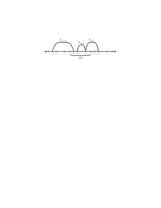
Figure 3: 0-branes on the cover of $S^{1}$ are indexed by two integers

The $U(\infty)$ theory describing the 0-branes on the covering space has a set of matrix degrees of freedom described by fields $X^{a}_{mi,nj}$. Such a field corresponds to a string stretching from the $m$th copy of 0-brane number $i$ to the $n$th copy of 0-brane number $j$. For simplicity of notation, we will suppress the $i,j$ indices and write these matrices as infinite matrices whose blocks $X^{a}_{mn}$ are themselves $N\times N$ matrices.

The constraint of translation invariance under $\Gamma={{Z}}$ imposes the condition that the theory is invariant under a simultaneous translation of the $X^{9}$ coordinate by $2\pi R_{9}$ and relabeling of the indices $n$ by $n+1$. Mathematically, this condition says that

$$X^{a}_{mn} = X^{a}_{(m-1)(n-1)},\;\;\;\;\;a<9$$

$$X^{9}_{mn} = X^{9}_{(m-1)(n-1)},\;\;\;\;\;m\neq n$$ (20)

$$X^{9}_{nn} = 2\pi R_{9}{\hbox to0.0pt{1\hss}\hskip 1.6pt\hbox{1}}+X^{9}_{(n-1)(n-1)}\ .$$

Note that the matrix added to $X^{9}_{nn}$ is proportional to the identity matrix. This is because the translation operation only shifts the diagonal components of the 0-brane matrices. An easy way to see this is that after $X^{9}$ has been diagonalized, its diagonal elements correspond to the positions of the branes in direction $X^{9}$; thus, adding a multiple of the identity matrix shifts the positions by a constant amount. Since the identity matrix commutes with everything, this is the correct implementation of the translation operation even when $X^{9}$ is not diagonal.

As a result of the constraints (20), the infinite block matrix $X^{9}_{mn}$ can be written in the following form

$$\left(\begin{array}[]{ccccccc}\ddots&X_{1}&X_{2}&X_{3}&\ddots\\ X_{-1}&X_{0}-2\pi R_{9}{\hbox to0.0pt{1\hss}\hskip 1.6pt\hbox{1}}&X_{1}&X_{2}&X_{3}\\ X_{-2}&X_{-1}&X_{0}&X_{1}&X_{2}\\ X_{-3}&X_{-2}&X_{-1}&X_{0}+2\pi R_{9}{\hbox to0.0pt{1\hss}\hskip 1.6pt\hbox{1}}&X_{1}\\ \ddots&X_{-3}&X_{-2}&X_{-1}&\ddots\end{array}\right)$$ (21)

where we have defined $X_{k}=X^{9}_{0k}$.

A matrix of this form can be interpreted as a matrix representation of the operator

$$X^{9}=i\hat{\partial}+A(\hat{x})$$ (22)

describing the action of a gauge covariant derivative on a Fourier decomposition of functions of the form

$$\phi(\hat{x})=\sum_{n}\hat{\phi}_{n}e^{in\hat{x}/\hat{R}_{9}}$$ (23)

which are periodic on a circle of radius $\hat{R}_{9}=\alpha^{\prime}/R_{9}=1/(2\pi R_{9})$. In order to see this correspondence concretely, let us first consider the action of the derivative operator $i\hat{\partial}$ on such a function. Writing the Fourier components as a column vector

$$\phi(\hat{x})\rightarrow\left(\begin{array}[]{c}\vdots\\ \hat{\phi}_{2}\\ \hat{\phi}_{1}\\ \hat{\phi}_{0}\\ \hat{\phi}_{-1}\\ \hat{\phi}_{-2}\\ \vdots\end{array}\right)$$ (24)

we find that the derivative operator acts as the matrix

$$i\hat{\partial}={\rm diag}(\ldots,-4\pi R_{9}{\hbox to0.0pt{1\hss}\hskip 1.6pt\hbox{1}},-2\pi R_{9}{\hbox to0.0pt{1\hss}\hskip 1.6pt\hbox{1}},0,2\pi R_{9}{\hbox to0.0pt{1\hss}\hskip 1.6pt\hbox{1}},4\pi R_{9}{\hbox to0.0pt{1\hss}\hskip 1.6pt\hbox{1}},\ldots).$$ (25)

This is precisely the inhomogeneous term along the diagonal of (21)

Decomposing the connection $A(\hat{x})$ into Fourier components in turn

$$A(\hat{x})=\sum_{n}A_{n}e^{in\hat{x}/\hat{R}_{9}}$$ (26)

we find that multiplication of $\phi(\hat{x})$ by $A(\hat{x})$ precisely corresponds in the matrix language to the action of the remaining part of (21) on the column vector representing $\phi(\hat{x})$, where $X_{n}=X_{0n}^{9}$ is identified with $A_{n}$.

This shows that we can identify

$$X^{9}\sim i\hat{\partial}^{9}+\hat{A}^{9}$$ (27)

under T-duality in the compact direction. This identification demonstrates that the infinite number of degrees of freedom in the matrix $X^{9}$ of a constrained $U(\infty)$ Matrix theory describing $N$ 0-branes on ${{R}}^{8}\times S^{1}$ can be precisely packaged in the degrees of freedom of a $U(N)$ connection on a dual circle $\hat{S}^{1}$ of radius $\hat{R}_{9}=1/(2\pi R_{9})$. A similar correspondence exists for the transverse degrees of freedom $X^{a}$, $a<9$, and for the fermion fields $\psi$. Because these fields are unchanged under the translation symmetry, the infinite matrices which they are described by in the 0-brane language satisfy condition (20) without the inhomogeneous term. Thus, these degrees of freedom simply become $N\times N$ matrix fields living on the dual $\hat{S}^{1}$ whose Fourier modes correspond to the winding modes of the original 0-brane fields.

This construction gives a precise correspondence between the degrees of freedom of the supersymmetric Matrix theory describing $N$ 0-branes moving on ${{R}}^{8}\times S^{1}$ and the $(1+1)$-dimensional super Yang-Mills theory on the dual circle. To show that the theories themselves are equivalent it only remains to check that the Lagrangian of the 0-brane theory is taken to the super Yang-Mills Lagrangian under this identification. In fact, this is quite easy to verify. Considering first the commutator terms, the term

$${\rm Tr}\;[X^{a},X^{b}]^{2}\;\;\;\;\;(a,b\neq 9)$$ (28)

in the 0-brane Matrix theory turns into the term

$$\frac{1}{2\pi\hat{R}_{9}}\int d\hat{x}\;{\rm Tr}\;[X^{a},X^{b}]^{2}$$ (29)

of 2D super Yang-Mills. Note that the trace in the 0-brane theory is a trace over the infinite index $n\in{{Z}}$ as well as over $i\in\{1,\ldots,N\}$. The trace over $n$ has the effect of extracting the Fourier zero mode of the corresponding product of fields in the dual theory. The factor of $R_{9}=1/(2\pi\hat{R}_{9})$ in front of the integral in the 2D super Yang-Mills is needed to normalize the zero mode so that it integrates to unity. Technically, there should be a factor of $1/|\Gamma|$ multiplying the 0-brane matrix Lagrangian because of the multiplicity of the copies; this factor is canceled by an overall factor of $|\Gamma|$ from the trace, and since both factors are infinite we simply drop them from all equations for convenience.

Now let us consider the commutator term when one of the matrices is $X^{9}$. In this case we have

$${\rm Tr}\;[X^{9},X^{a}]^{2}$$ (30)

which becomes after the replacement (27)

$$-\left(\frac{1}{2\pi\hat{R}_{9}}\right)\int d\hat{x}\;{\rm Tr}\;(\partial_{9}X^{a}-i[A_{9},X^{a}])^{2}=-\left(\frac{1}{2\pi\hat{R}_{9}}\right)\int d\hat{x}\;{\rm Tr}\;(D_{9}X^{a})^{2}$$ (31)

which is precisely the derivative squared term for the adjoint scalars which we expect in the dual 1-brane theory.

The kinetic term for $X^{9}$ in the 0-brane theory becomes the Yang-Mills curvature squared term in the dual theory

$${\rm Tr}\;(D_{0}X^{9})^{2}\rightarrow\left(\frac{1}{2\pi\hat{R}_{9}}\right)\int d\hat{x}\;{\rm Tr}\;F_{09}^{2}\ .$$ (32)

The remaining terms in the 0-brane Lagrangian transform straightforwardly into precisely the remaining terms expected in a 2D super Yang-Mills Lagrangian with 16 supercharges. This shows that there is a rigorous equivalence between the low-energy field theory description of $N$ 0-branes on ${{R}}^{8}\times S^{1}$ and the low-energy field theory description of $N$ 1-branes wrapped around a dual $\hat{S}^{1}$ in the static gauge. We note again the fact that the Lagrangian in the dual Yang-Mills theory carries an overall multiplicative factor of the original radius $R_{9}$. This fact will play a significant role in later discussions, particularly in regard to Matrix theory. The fact that the coupling constant in the dual Lagrangian should correspond with that of (7) for a system of 1-branes indicates that under T-duality the string coupling transforms through $\hat{g}=g\sqrt{\alpha^{\prime}}/R_{9}$, which is what we expect from string theory.

3.1.2   $p$-branes on a torus $T^{d}$

So far we have discussed the situation of $N$ 0-branes moving on a space which has been compactified in a single direction. It is straightforward to generalize this argument to $p$-branes of arbitrary dimension moving in a space with any number of compact dimensions. By carrying out the construction described above for each of the compact directions in turn, it can be shown that the low-energy theory of $N$ $p$-branes which are completely unwrapped on a torus $T^{d}$ is equivalent to the low-energy theory of $N$ $(p+d)$-branes which are wrapped around the torus, in static gauge. The only new type of term which appears in the Lagrangian corresponds to a commutator term for two directions which are both compactified. In the original $p$-brane theory, such a term would appear as $[X^{a},X^{b}]^{2}$ (integrated over the $p$-dimensional volume of the brane). After T-duality on the two compact directions this term becomes

$$-\left(\frac{1}{4\pi^{2}\hat{R}_{a}\hat{R}_{b}}\right)\int d\hat{x}^{a}d\hat{x}^{b}\;(F^{ab})^{2}$$ (33)

which is just the appropriate Yang-Mills curvature strength squared term in the dual theory. Note that in the dual theory, the action is multiplied by a factor of $R_{a}R_{b}$, since each compact direction gives an extra factor of the radius.

As a particular example of compactification on a higher dimensional torus, we can consider the theory of $N$ 0-branes on a torus $T^{d}$. After interpreting the winding modes of each matrix in terms of Fourier modes of a dual theory, it follows that the Lagrangian becomes precisely that of super Yang-Mills theory in $d+1$ dimensions with a Yang-Mills coupling constant $g_{YM}$ proportional to $V^{-1/2}$ where $V$ is the volume of the original torus $T^{d}$.

3.1.3   Further comments regarding T-duality

Throughout this section we have fixed the constant $2\pi\alpha^{\prime}=1$. It will be useful in some of the later discussions to have the appropriate factors of $\alpha^{\prime}$ reinstated in (27). This is quite straightforward; since $\alpha^{\prime}$ has units of length squared, the correct T-duality relation is given by

$$X^{a}\leftrightarrow(2\pi\alpha^{\prime})(i\partial^{a}+A_{a})$$ (34)

where $X^{a}$ represents an infinite matrix of fields including winding strings around a compactified dimension, and $A$ represents a connection on a gauge bundle over the dual circle.

It should be emphasized that this T-duality relation gives a precise correspondence between winding modes of strings on the original circle and momentum modes on the dual circle. This is precisely the association expected from T-duality in perturbative string theory [?].

So far we have been discussing field configurations in the $X^{a}$ matrices which correspond in the dual picture to connections on a $U(N)$ bundle with trivial boundary conditions. In fact, there are also twisted sectors in the theory corresponding to bundles with nontrivial boundary conditions. We will now discuss such configurations briefly. To make the story clear, it is useful to reformulate the above discussion in a slightly more abstract language.

The constraints (20) can be formulated by saying that there exists a translation operator $U$ under which the infinite matrices $X^{a}$ transform as

$$UX^{a}U^{-1}=X^{a}+\delta^{a9}2\pi R_{9}{\hbox to0.0pt{1\hss}\hskip 1.6pt\hbox{1}}.$$ (35)

This relation is satisfied formally by the operators

$$X^{9}=i\partial^{9}+A_{9},\;\;\;\;\;\;\;\;\;\;U=e^{2\pi i\hat{x}^{9}R_{9}}$$ (36)

which correspond to the solutions discussed above. In this formulation of the quotient theory, the operator $U$ generates the group $\Gamma={{Z}}$ of covering space transformations. Generally, when we take a quotient theory of this type, however, there is a more general constraint which can be satisfied. Namely, the translation operator only needs to preserve the state up to a gauge transformation. Thus, we can consider the more general constraint

$$UX^{a}U^{-1}=\Omega(X^{a}+\delta^{a9}2\pi R_{9}{\hbox to0.0pt{1\hss}\hskip 1.6pt\hbox{1}})\Omega^{-1}.$$ (37)

where $\Omega\in U(N)$ is an arbitrary element of the gauge group. This relation is satisfied formally by

$$X^{9}=i\partial^{9}+A_{9},\;\;\;\;\;\;\;\;\;\;U=\Omega\cdot e^{2\pi i\hat{x}^{9}R_{9}}$$ (38)

This is precisely the same type of solution as we have above; however, there is the additional feature that the translation operator now includes a nontrivial gauge transformation. On the dual circle $\hat{S}^{1}$ this corresponds to a gauge theory on a bundle with a nontrivial boundary condition in the compact direction 9. Note that even with such a nontrivial boundary condition, any $U(N)$ bundle over $S^{1}$ is topologically trivial. An example of the type of boundary condition which might appear would be to take $\Omega$ to be a permutation in $S_{N}$. This type of gauge transformation has the effect in the original 0-brane theory of switching the labels of the 0-branes on each sheet of covering space. When translated into the dual gauge theory picture, this corresponds to a super Yang-Mills theory with a nontrivial boundary condition $\Omega$ in the compact direction.

A similar story occurs when several directions are compact. In this case, however, there is a constraint on the translation operators in the different compact directions. For example, if we have compactified on a 2-torus in dimensions 8 and 9, the generators $U_{8}$ and $U_{9}$ of a general twisted sector must generate a group isomorphic to ${{Z}}^{2}$ and therefore must commute. The condition that these generators commute can be related to the condition that the boundary conditions in the dual gauge theory correspond to a well-defined $U(N)$ bundle over the dual torus. For compactifications in more than one dimension such boundary conditions can define a topologically nontrivial bundle. In Section 4 we will discuss nontrivial bundles of this nature in much more detail. It is interesting to note that this construction can even be generalized to situations where the generators $U_{i}$ do not commute. This leads to a dual theory which is described by gauge theory on a noncommutative torus [?, ?, ?].

3.2 S-duality for strings and super Yang-Mills

The T-duality symmetry we have discussed above is a symmetry of type II string theory which is essentially perturbative, in the sense that the string coupling is only changed through multiplication by a constant. Another remarkable symmetry seems to exist in the type II class of theories which is essentially nonperturbative; this is the S-duality symmetry of the type IIB string [?, ?]. S-duality is a symmetry which acts according to the group $SL(2,{{{Z}}})$ on the type IIB theory. At the level of the low-energy IIB supergravity theory, the dilaton and axion form a fundamental $SL(2,{{Z}})$ multiplet, as do the NS-NS and R-R two-forms. Because the string coupling $g$ is given by the exponential of the dilaton, this S-duality is a nonperturbative symmetry which can exchange strong and weak couplings. Because symmetries in the S-duality group exchange the NS-NS and R-R two-forms, we can see that S-duality exchanges strings and D1-branes, and also exchanges D5-branes and NS (solitonic) 5-branes. As there is only a single four-form in the IIB theory, however, it must be left invariant under S-duality; it follows that S-duality takes a D3-brane into another D3-brane.

Since D3-branes are invariant under S-duality, it is interesting to ask how we can understand the action of S-duality on the low-energy field theory describing $N$ parallel D3-branes. This field theory is the reduction to four dimensions of $U(N)\;{\cal N}=1$ SYM in 10D, which is the pure $U(N)$ ${\cal N}=4$ super Yang-Mills theory in 3 + 1 dimensions. Since the Yang-Mills coupling of this theory is related to the string coupling through $g_{YM}^{2}\sim g$, the action of S-duality on this super Yang-Mills theory must be a nonperturbative $SL(2,{{Z}})$ duality symmetry. In fact, for a number of years it has been conjectured that 4D super Yang-Mills theory with ${\cal N}=4$ supersymmetry has precisely such an S-duality symmetry. This is a supersymmetric version of the non-abelian S-duality symmetry proposed originally by Montonen and Olive. We will now briefly review the basics of this duality symmetry.

Maxwell’s equations describe a simple non-supersymmetric $U(1)$ gauge theory in four dimensions. In the absence of sources, these equations have a very simple symmetry, which takes the curvature tensor $F$ to its dual $*F$. This has the effect of exchanging the electric and magnetic fields in the theory (up to signs). Although this symmetry is broken when electric sources are introduced, if magnetic sources are also introduced then the symmetry is maintained when the electric and magnetic charges are also exchanged.

This marvelous symmetry of $U(1)$ gauge field theory seems at first sight to break down for non-abelian theories with gauge groups like $U(N)$. It was suggested, however, by Montonen and Olive [?] that such a symmetry might be possible for non-abelian theories if the gauge group $G$ were replaced by a dual group $\hat{G}$ with a dual weight lattice. Further work [?, ?] indicated that such a non-abelian duality symmetry would probably only be possible in theories with supersymmetry, and that the ${\cal N}=4$ theory was the most likely candidate. Although there is still no complete proof that the ${\cal N}=4$ super Yang-Mills theory in 4D has this S-duality symmetry, there is a growing body of evidence which supports this conclusion.

The proposed non-abelian S-duality symmetry of 4D super Yang-Mills acts by the group $SL(2,{{Z}})$, just as we would expect from string theory. The (rescaled) Yang-Mills coupling constant and theta angle can be conveniently packaged into the quantity

$$\tau=\frac{\theta}{2\pi}+\frac{i}{g_{{\rm YM}}^{2}}$$ (39)

which is transformed under $SL(2,{{{Z}}})$ by the standard transformation law

$$\tau\rightarrow\frac{a\tau+b}{c\tau+d}$$ (40)

where $a,b,c,d\in{{{Z}}}$ with $ad-bc=1$ parameterize a matrix

$$\left(\begin{array}[]{cc}a&b\\ c&d\end{array}\right)$$ (41)

in $SL(2,{{Z}})$. In particular, the group $SL(2,{{Z}})$ is generated by the transformations

$$\tau\rightarrow\tau+1$$ (42)

corresponding to the periodicity of $\theta$, and

$$\tau\rightarrow-1/\tau$$ (43)

which inverts the coupling and corresponds to strong-weak duality.

There is by now a large body of evidence that S-duality is a true symmetry of ${\cal N}=4$ super Yang-Mills. However, to date there is no real proof of S-duality from the point of view of field theory. One of the strongest pieces of evidence for this duality symmetry is the fact that the spectrum of supersymmetric bound states of dyons is invariant under the action of the S-duality group; a detailed proof of this result and further references can be found in [?].

4 Branes and Bundles

As we discussed in Section 3.1.3, there are different topological sectors for a system of 0-branes on a torus which correspond in the dual gauge theory language to nontrivial $U(N)$ bundles over the dual torus. In fact, these topologically nontrivial configurations of branes correspond to systems containing not only the original 0-branes but also branes of higher dimension. In this section we describe in some detail a general feature of D-branes which amounts to the fact that the low-energy Yang-Mills theory describing Dirichlet $p$-branes also contains information about D-branes of both higher and lower dimensions. Roughly speaking, D-branes of lower dimension can be described by topologically nontrivial configurations of the $U(N)$ gauge field living on the original $p$-branes, while D-branes of higher dimension can be encoded in nontrivial commutation relations between the matrices $X^{a}$ describing transverse D-brane excitations in compact directions. In order to make the discussion precise, it will be useful to begin with a review of nontrivial gauge bundles on compact manifolds. In these notes we will concentrate primarily on configurations of D-branes on tori; on general compact spaces the story is similar but there are some additional subtleties [?, ?, ?, ?].

4.1 Review of vector bundles

An introductory review of bundles and their relevance for gauge field theory is given in [?]. In this section we briefly review some salient features of bundles and Yang-Mills connections. Roughly speaking, a (real) vector bundle is a space constructed by gluing together a copy of a vector space $V={{R}}^{k}$ (called the fiber space) for each point on a particular manifold $M$ (called the base manifold) in a smooth fashion. Mathematically speaking, a vector bundle can be defined by decomposing $M$ into coordinate patches $U_{i}$. The vector bundle is locally equivalent to $U_{i}\times{{R}}^{k}$. When the patches of $M$ are glued together, however, there can be nontrivial identifications which give the vector bundle a nontrivial topology. For every pair of intersecting patches $U,V$ there is a transition function between these patches which relates the fibers at each common point. Such a transition function $\Omega_{UV}$ takes values in a group $G$ called the structure group of the bundle. The transition function $\Omega_{UV}$ identifies $(u,f^{\prime})$ and $(v,f)$ where $u$ and $v$ are points in $U$ and $V$ which represent the same point in $M$, and where the fiber elements are related through $f^{\prime}=\Omega_{UV}f$.

In order to describe a well-defined bundle, the transition functions must obey certain relations called cocycle conditions. For example, if as in Figure 4 there are three patches $U,V,W$ whose intersection is nonempty, the transition functions between the three patches must obey the relation

$$\Omega_{UV}\Omega_{VW}\Omega_{WU}={\rm id}$$ (44)

where ${\rm id}$ is the identity element in $G$. This is clearly necessary in order that a point $(u,f)$ in the intersection region not be identified with any other point in the same fiber after repeated application of the transition functions.

Figure 4: Three patches on a manifold $M$ over which a bundle is defined

This describes a bundle whose fiber is a vector space. Another type of bundle, called a principal bundle, has a fiber which is a copy of the structure group $G$ itself. A Yang-Mills connection for a gauge theory with gauge group $G$ is associated with a principal bundle with fiber $G$. Formally speaking, a Yang-Mills connection $A_{\mu}$ is a one-form which takes values in the Lie algebra of $G$. A connection of this type gives a definition of parallel transport in the bundle. The most important feature for our purposes is the transformation property of such a connection under a transition function $\Omega$, which is given by

$$A^{\prime}=\Omega\cdot A\cdot\Omega^{-1}-i\;d\Omega\cdot\Omega^{-1}$$ (45)

Generally, a physical theory will include both a Yang-Mills field and additional matter fields. The Yang-Mills connection is defined with respect to a particular principal bundle, and the matter fields are given by sections of associated vector bundles whose transition functions are given by particular representations of the $G$-valued transition functions of the principal bundle.

Over any compact Euclidean manifold, such as the torus $T^{d}$, there are many topologically inequivalent ways to construct a nontrivial bundle. One way to distinguish such inequivalent bundles is through the use of topological invariants called characteristic classes. One of the simplest examples of characteristic classes are the Chern classes. These classes distinguish topologically inequivalent $U(N)$ bundles, and are given by invariant polynomials in the Yang-Mills field strength

$$F_{\mu\nu}=\partial_{\mu}A_{\nu}-\partial_{\nu}A_{\mu}-i[A_{\mu},A_{\nu}].$$ (46)

The first two Chern classes are defined by

$$c_{1} = \frac{1}{2\pi}{\rm Tr}\;F$$ (47)

$$c_{2} = \frac{1}{8\pi^{2}}\left({\rm Tr}\;F\wedge F-({\rm Tr}\;F)\wedge({\rm Tr}\;F)\right)$$

These forms $c_{i}$ are integral cohomology classes, so that when $c_{i}$ is integrated over any $2i$-dimensional submanifold (homology class) the result is an integer. As we will now discuss, in a low-energy D-brane Yang-Mills theory, these integers count lower-dimensional D-branes embedded in the original D-brane world-volume.

4.2 D-branes from Yang-Mills curvature

Let us consider the low-energy Yang-Mills theory describing $N$ coincident $p$-branes. If the bundle associated with the Yang-Mills connection is nontrivial, this indicates that the gauge field configuration carries R-R charges which are associated with D-branes of dimension less than $p$. We will now formulate precisely the way in which these lower-dimensional D-branes appear, after which we will discuss the justification for these statements.

Simply put, the integral form corresponding to the $k$th antisymmetric product of the curvature form $F$ carries $(p-2k)$-brane charge. Thus,

$$\frac{1}{2\pi}\int{\rm Tr}\;F {\rm corresponds\ to}\;(p-2)-{\rm brane\ charge}.$$

$$\frac{1}{8\pi^{2}}\int{\rm Tr}\;(F\wedge F) {\rm corresponds\ to}\;(p-4)-{\rm brane\ charge}.$$

$$\frac{1}{48\pi^{3}}\int{\rm Tr}\;(F\wedge F\wedge F) {\rm corresponds\ to}\;(p-6)-{\rm brane\ charge,\ etc.}\ldots$$

More precisely, let us imagine that a $(p-2)$-brane is wrapped around some $(p-2)$-dimensional homology cycle $h_{p-2}$ in the $p$-dimensional volume of the original $p$-branes. If we choose any two-dimensional cycle $h_{2}$, it will generically intersect $h_{p-2}$ in a fixed number of points, corresponding to the intersection number of these two cycles. Thus, any $(p-2)$-cycle defines a cohomology class which associates an integer with any 2-cycle. This cohomology class is known as the Poincare dual of the original homology class. Using this correspondence we can state the connection between D-branes and field strength precisely: The integral cohomology class proportional to $F\wedge^{k}F$ is the Poincare dual of a $(p-2k)$-dimensional homology class which describes a system of embedded $(p-2k)$-branes.

The observation that the instanton number $\frac{1}{8\pi^{2}}\int F\wedge F$ carries $(p-4)$-brane charge was first made by Witten in the context of 5-branes and 9-branes [?]. The more general result for arbitrary $p,k$ was described by Douglas [?]. From the string theory point of view, this correspondence between D-branes and Yang-Mills curvature arises from a Chern-Simons type of term which appears in the full D-brane action, and is given by [?]

$${\rm Tr}\;\int_{\Sigma_{p+1}}{\cal A}\wedge e^{F}$$ (48)

where ${\cal A}$ is a sum over all the R-R fields

$${\cal A}=\sum_{k}A^{(k)}$$ (49)

and where the integral is taken over the full $(p+1)$-dimensional world-volume of the $p$-brane. For example, on a 4-brane $F\wedge F$ couples to $A^{(1)}$ through

$${\rm Tr}\;\int_{\Sigma_{5}}A^{(1)}\wedge F\wedge F,$$ (50)

demonstrating that $F\wedge F$ is playing the role of 0-brane charge in this case. The existence of the Chern-Simons term (48) can be shown on the basis of anomaly cancellation arguments [?]. It is also possible, however, to show that these terms must appear simply using the principles of T-duality and rotational invariance [?, ?, ?, ?]. We follow the latter approach here; in the following sections we show how the correspondence between lower-dimensional branes and wedge products of the curvature form can be seen directly in the low-energy Yang-Mills description of D-branes, using only T-duality and the intrinsic properties of Yang-Mills theory.

4.3 Bundles over tori

We will be primarily concerned here with D-branes on toroidally compactified spaces. Thus, it will be useful to explicitly review here some of the properties of $U(N)$ bundles over tori. Let us begin with the simplest case, the two-torus $T^{2}$.

If we consider a space which has been compactified on $T^{2}$ with radii

$$R_{1}=L_{1}/(2\pi),\;R_{2}=L_{2}/(2\pi)$$ (51)

then the low-energy field theory of $N$ wrapped 2-branes is $U(N)$ SYM on $T^{2}$. To describe a $U(N)$ bundle over a general manifold, we need to choose a set of coordinate patches on the manifold. For the torus, we can choose a single coordinate patch covering the entire space, where the transition functions for the bundle are given by (see Figure 5)

Figure 5: Transition functions defining a bundle over the 2-torus

$$\Omega_{1}(x_{2}),\;\Omega_{2}(x_{1}).$$ (52)

A connection on a bundle defined by these transition functions must obey the boundary conditions

$$A_{1}(x_{1}+L_{1},x_{2}) = \Omega_{1}(x_{2})A_{1}(x_{1},x_{2})\Omega_{1}^{-1}(x_{2})$$ (53)

$$A_{2}(x_{1}+L_{1},x_{2}) = \Omega_{1}(x_{2})A_{2}(x_{1},x_{2})\Omega_{1}^{-1}(x_{2})-i\;(\partial_{2}\Omega_{1}(x_{2}))\cdot\Omega^{-1}_{1}(x_{2})$$

$$A_{1}(x_{1},x_{2}+L_{2}) = \Omega_{2}(x_{1})A_{1}(x_{1},x_{2})\Omega_{2}^{-1}(x_{1})-i\;(\partial_{1}\Omega_{2}(x_{1}))\cdot\Omega^{-1}_{2}(x_{1})$$

$$A_{2}(x_{1},x_{2}+L_{2}) = \Omega_{2}(x_{1})A_{2}(x_{1},x_{2})\Omega_{2}^{-1}(x_{1})$$

while a matter field $\phi$ in the fundamental representation must satisfy the boundary conditions

$$\phi(x_{1}+L_{1},x_{2}) = \Omega_{1}(x_{2})\phi(x_{1},x_{2})$$

$$\phi(x_{1},x_{2}+L_{2}) = \Omega_{2}(x_{1})\phi(x_{1},x_{2}).$$ (54)

The cocycle condition for a well-defined $U(N)$ bundle is

$$\Omega_{1}(L_{2})\Omega_{2}(0)\Omega_{1}^{-1}(0)\Omega_{2}^{-1}(L_{1})={\hbox to0.0pt{1\hss}\hskip 1.6pt\hbox{1}}.$$ (55)

In general, $U(N)$ bundles over $T^{2}$ are classified by the first Chern number

$$C_{1}=\int c_{1}=\frac{1}{2\pi}\int{\rm Tr}\;F=k\in{{{Z}}}$$ (56)

Physically, this integer corresponds to the total non-abelian magnetic flux on the torus. In order to understand these nontrivial $U(N)$ bundles, it is helpful to decompose the gauge group into its abelian and non-abelian components

$$U(N)=(U(1)\times SU(N))/{{{Z}}}_{N}.$$ (57)

Because the curvature $F$ has a trace which arises purely from the abelian part of the gauge group, we see that the $U(1)$ part of the total field strength for a bundle with $C_{1}=k$ is given by $F=k{\hbox to0.0pt{1\hss}\hskip 1.6pt\hbox{1}}/N$. Such a field strength would not be possible for a purely abelian theory (assuming the existence of matter fields in the fundamental representation) since it would not be possible to satisfy (55). Once $U(1)$ is embedded in $U(N)$ through (57), however, this deficiency can be corrected by choosing $SU(N)$ boundary conditions $\tilde{\Omega}$ which correspond to a “twisted” bundle. Such boundary conditions satisfy

$$\tilde{\Omega}_{1}(L_{2})\tilde{\Omega}_{2}(0)\tilde{\Omega}_{1}^{-1}(0)\tilde{\Omega}_{2}^{-1}(L_{1})=Z$$ (58)

where $Z=e^{-2\pi ik/N}{\hbox to0.0pt{1\hss}\hskip 1.6pt\hbox{1}}$ is central in $SU(N)$. Twisted bundles of this type were originally considered by ’t Hooft [?].

The integer $k$ gives a complete classification of $U(N)$ bundles over $T^{2}$. Over a higher dimensional torus $T^{n}$, the story is essentially the same, however there is an integer $k_{ij}$ for every pair of dimensions in the torus. For each dimension $i$ there is a transition function, and for each pair $i,j$ the transition functions satisfy a cocycle relation of the form (55).

4.4 Example: 0-branes as flux on $T^{2}$

We will now discuss nontrivial bundles on $T^{2}$ and show using T-duality that the first Chern class indeed counts 0-branes.

Consider a $U(N)$ theory on $T^{2}$ with total flux $\int{\rm Tr}\;F=2\pi$. We can choose an explicit set of boundary conditions corresponding to such a bundle

$$\Omega_{1}(x_{2}) = e^{2\pi i(x_{2}/L_{2})T}V$$ (59)

$$\Omega_{2}(x_{1}) =$$ 1 1

where

$$V=\pmatrix{&1&&&\cr&&1&&\cr&&&\ddots&\cr&&&&1\cr 1&&&&}$$ (60)

and $T={\rm Diag}\;(0,0,\ldots,0,1)$.

To understand the D-brane geometry of this bundle, let us construct a linear connection on the bundle, which will correspond in the T-dual picture to flat D-branes on the dual torus. The boundary conditions (59) admit a linear connection with constant curvature

$$\begin{array}[]{lll}A_{1}&=&0\\ A_{2}&=&Fx_{1}+\frac{2\pi}{L_{2}}\;{\rm Diag}(0,1/N,\ldots,(N-1)/N)\end{array}$$ (61)

with

$$F=\frac{2\pi}{NL_{1}L_{2}}{\hbox to0.0pt{1\hss}\hskip 1.6pt\hbox{1}}.$$ (62)

Because we have chosen the boundary conditions such that $\Omega_{2}=1$ we can T-dualize in a straightforward fashion using $X^{2}=(2\pi\alpha^{\prime})(i\partial_{2}+A_{2})$. After such a T-duality, $X^{2}$ represents the transverse positions of a set of 1-branes on $T^{2}$. This field is represented by an infinite matrix with indices $n\in{{Z}}$ and $i\in\{1,\ldots,N\}$. In the $(n,m)=(0,0)$ block, the field $X^{2}$ is given by the matrix

$$X^{2}=\left(\frac{\hat{L}_{2}}{N}\right)\left(\begin{array}[]{cccc}\frac{x_{1}}{L_{1}}&0&0&\ddots\\ 0&\frac{x_{1}}{L_{1}}+1&0&\ddots\\ 0&0&\ddots&0\\ \ddots&\ddots&0&\frac{x_{1}}{L_{1}}+(N-1)\end{array}\right)$$ (63)

where

$$\hat{L}_{2}=\frac{4\pi^{2}\alpha^{\prime}}{L_{2}}$$ (64)

Thus, we see that the T-dual of the original gauge field on $T^{2}$ describes a single 1-brane wrapped once diagonally around $\hat{R}_{2}$, and $N$ times around $R_{1}$ (See Figure 6).

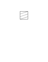
Figure 6: An $(N,1)$ diagonally wrapped string dual to $N$ 2-branes with one unit of flux

The dual configuration has quantum numbers corresponding to $N$ 1-branes on $R_{1}$ and a single 1-brane on $\hat{R}_{2}$. In homology this state could be written as

$$N\cdot(1)+(2)$$ (65)

Since wrapped 1-branes are T-dual to 0-branes, the original flux on the 2-brane corresponds to a single 0-brane. This gives a simple geometrical demonstration through T-duality of the result that the first Chern class counts $(p-2)$-branes.

It is straightforward to carry out an analogous construction for a system with $k$ 0-branes. In this case, the nontrivial boundary condition becomes [?]

$$\Omega_{1}(x_{2})=e^{2\pi i(x_{2}/L_{2})T}V^{k}$$ (66)

with $T$ being the diagonal matrix

$$T = {\rm Diag}(n,\ldots,n,n+1,\ldots,n+1)$$ (67)

where $n$ is the integral part of $k/N$ and where the multiplicities of the diagonal elements of $T$ are $N-k$ and $k$ respectively.

In the discussion in this section we have chosen to set $\Omega_{2}=1$ for convenience. This makes the discussion slightly simpler since the T-duality relation in direction 2 is implemented directly through (34). For a nontrivial gauge transformation $\Omega_{2}$ T-duality would give a configuration of the type described by (37). For example, if we used the more standard (’t Hooft type) boundary conditions for the bundle with $k=1$

$$\Omega_{1}(x_{2}) = e^{2\pi i(x_{2}/L_{2})(1/N)}U$$ (68)

$$\Omega_{2}(x_{1}) = V$$

where

$$U=\pmatrix{1&&&\cr&e^{2\pi i\over N}&&\cr&&\ddots&\cr&&&e^{2\pi i(N-1)\over N}}$$ (69)

Then after T-duality in direction 2 we would get a 1-brane configuration in which translation by $2\pi\hat{R}_{2}$ in the covering space would give rotation by $V$, permuting the labels on the 1-branes. This situation is gauge equivalent to the one we have discussed where the boundary conditions are given by (59).

4.5 Example: 0-branes as instantons on $T^{4}$

Let us now consider nontrivial bundles on $T^{4}$. From the previous discussion it is clear that a nonvanishing first Chern class indicates the existence of 2-branes in the system. For example, if $\int F_{12}=2\pi$ then the configuration contains a 2-brane wrapped around the (34) homology cycle. A constant curvature connection with $\int F_{12}=2\pi$ and $\int F_{34}=2\pi$ would correspond after T-duality in directions 2 and 4 to a diagonally wrapped 2-brane, and in the original Yang-Mills theory on $T^{4}$ corresponds to a “4-2-2-0” configuration with a unit of 0-brane charge as well as 2-brane charge in directions $(12)$ and $(34)$ [?]. A more interesting configuration to consider is one where the first Chern class vanishes but the second Chern class does not. This corresponds to an instanton in the $U(N)$ gauge theory on $T^{4}$. To consider an explicit example of such a configuration, let us take a $U(N)$ gauge theory on a torus $T^{4}$ with sides all of length $L$. We want to construct a bundle with nontrivial second Chern class $C_{2}=(8\pi^{2})^{-1}\int c_{2}=k$ and with $c_{1}=0$. There is no smooth $U(N)$ instanton with $k=1$; a single instanton tends to shrink to a point on the torus [?]. Thus, we will consider a configuration with $k=2,N=2$.

To construct a bundle with the desired topology we can take the transition functions in the four directions of the torus to be

$$\Omega_{2}=\Omega_{4} =$$ 1 1

$$\Omega_{1} = e^{2\pi i(x_{2}/L)\tau_{3}}$$ (70)

$$\Omega_{3} = e^{2\pi i(x_{4}/L)\tau_{3}}$$

where

$$\tau_{3}=\left(\begin{array}[]{cc}1&0\\ 0&-1\end{array}\right)$$ (71)

is the usual Pauli matrix. This bundle admits a linear connection

$$A_{1}=A_{3} = 0$$

$$A_{2} = \frac{2\pi x_{1}}{L^{2}}\tau_{3}$$ (72)

$$A_{4} = \frac{2\pi x_{3}}{L^{2}}\tau_{3}$$

whose curvature is given by

$$F_{12}=F_{34} = \frac{2\pi}{L^{2}}\tau_{3}$$ (73)

Since ${\rm Tr}\;F=0$ there is no net 2-brane charge, as desired. The instanton number of the bundle is

$$C_{2}=\frac{1}{8\pi^{2}}\int d^{4}x\;{\rm Tr}\;F\wedge F=2.$$ (74)

As we would expect from the discussion in section 4.2, this should correspond to the existence of two 0-branes in the system. We can see this by again using T-duality. After performing T-duality transformations in directions 2 and 4 we get two 2-branes whose transverse coordinates are described by

$$X^{2}(x_{1},x_{3}) = \pm\hat{L}x_{1}/L$$ (75)

$$X^{4}(x_{1},x_{3}) = \pm\hat{L}x_{3}/L$$

where $\hat{L}=4\pi^{2}\alpha^{\prime}/L$. These 2-branes are wrapped diagonally on the dual $T^{4}$ in such a way that they correspond to the following homology 2-cycles

$${\rm brane\ 1} \rightarrow (13)+(14)+(23)+(24)$$ (76)

$${\rm brane\ 2} \rightarrow (13)-(14)-(23)+(24)$$

The total resulting homology class is $2(13)+2(24)$, which is T-dual to two 4-branes and two 0-branes as expected. Further discussion of configurations of this type which are dual to instantons on $T^{4}$ can be found in [?, ?, ?].

4.6 Branes from lower-dimensional branes

In the preceding subsections we have discussed how, in general, $(p-2k)$-branes can be described by nontrivial gauge configurations in the world-volume of a system of parallel $p$-branes. We will now discuss the T-dual interpretation of this result, which indicates that it is equally possible to construct $(p+2k)$-branes out of a system of interacting $p$-branes by choosing noncommuting matrices to describe the transverse coordinates.

In the context of the preceding discussion, it is easiest to describe the construction of higher-dimensional branes from a finite number of $p$-branes in the case of toroidally compactified space. In Sections 7.2.2 and 7.2.3 we will discuss the construction of higher dimensional branes in noncompact spaces from a system of 0-branes. The simplest example of the phenomenon we wish to discuss here is the description of a 2-brane in terms of a “topological” charge associated with the matrices describing $N$ 0-branes on $T^{2}$. To see how a configuration with such a charge is constructed, consider again the diagonal ($N,1$) 1-brane on $T^{2}$ (Figure 6). If we take the toroidal dimensions to be $L_{1}\times L_{2}$ then the diagonal 1-brane configuration satisfies

$$[(\partial_{1}-iA_{1}),X^{2}]=\frac{L_{2}}{NL_{1}}{\hbox to0.0pt{1\hss}\hskip 1.6pt\hbox{1}}.$$ (77)

By taking the T-dual on $X^{2}$ we get a system of $N$ 2-branes with unit flux

$$[(\partial_{1}-iA_{1}),(\partial_{2}-iA_{2})]=-iF=\frac{-2\pi i}{NL_{1}\hat{L}_{2}}{\hbox to0.0pt{1\hss}\hskip 1.6pt\hbox{1}},$$ (78)

as discussed in Section 4.4. If, on the other hand, we perform a T-duality transformation on $X^{1}$, then we get a system of $N$ 0-branes satisfying

$$[X^{1},X^{2}]=\frac{2\pi\hat{R}_{1}R_{2}i}{N}{\hbox to0.0pt{1\hss}\hskip 1.6pt\hbox{1}}$$ (79)

where $\hat{R}_{1}$ and $R_{2}$ are the radii of the torus on which the 0-branes are moving. Since the 1-brane wrapped around $X^{2}$ becomes a 2-brane on $T^{2}$ under the T-duality transformation which takes the 1-branes on $X^{1}$ to 0-branes, we see that on a $T^{2}$ with area $A$ a system of $N$ 0-branes described by (infinite) matrices $X$ satisfying

$${\rm Tr}\;[X^{1},X^{2}]=\frac{iA}{2\pi}$$ (80)

carries a unit of 2-brane charge. Note that if the 0-branes were not moving on a compact space the quantity in (80) would vanish for $N$ finite. In the infinite $N$ limit, however, as will be discussed in 7.2.2, this charge can be nonzero even in Euclidean space.

This discussion generalizes naturally to higher dimensions. For example, a system of $N$ 0-branes on a $T^{4}$ of volume $V$ with

$${\rm Tr}\;\epsilon_{abcd}X^{a}X^{b}X^{c}X^{d}=\frac{V}{2\pi^{2}}$$ (81)

will carry a unit of 4-brane charge [?, ?]. This is just the T-dual of the instanton number for a system of $N$ 4-branes, which is associated with 0-brane charge as discussed above. Similarly, any system of $p$-branes on a $2k$-dimensional transverse torus can be in a state with $(p+2k)$-brane charge.

It is also, of course, possible to mix the two types of conditions we have discussed to describe, for example, 2-brane charge on the (34) homology cycle of a 4-torus in terms of a gauge theory of 2-branes wrapped on the (12) homology cycles. Such a charge is proportional to

$${\rm Tr}\;\left(F_{12}[X^{3},X^{4}]-(D_{1}X^{3})(D_{2}X^{4})+(D_{1}X^{4})(D_{2}X^{3})\right).$$ (82)

4.7 Strings and electric fields

We have seen that the gauge fields and transverse coordinates of a system of $p$-branes can be combined to give $(p\pm 2k)$-brane charge. It is also possible to choose gauge fields on the world-volume of a $p$-brane which describe fundamental strings. Consider a system of 0-branes moving on a space which has been compactified in direction $X^{9}$. Clearly, these 0-branes can be given momentum in the compact direction; this momentum is proportional to $\dot{X}^{9}$ and is quantized in units of $1/R$. Under T-duality on the $S^{1}$, we have

$$\dot{X^{9}}\rightarrow\int(2\pi\alpha^{\prime})\dot{A_{9}}$$ (83)

Thus, momentum of a set of 0-branes corresponds to electric flux around the compact direction in the dual gauge theory. Since string momentum is T-dual to string winding, we see that electric flux in a gauge theory on a compact space can be associated with fundamental string winding number. It is natural to give this result a local interpretation, so that lines of electric flux in a gauge theory correspond to fundamental strings even in noncompact space.

It is interesting to note that 0-brane momentum in a compact direction and the T-dual string winding number are quantized only because of the quantum nature of the theory. On the other hand, the quantization of flux giving 0-brane charge in a gauge theory on $T^{2}$ arises from topological considerations, namely the fact that the first Chern class of a $U(1)$ bundle is necessarily integral. Nonetheless, in string theory these quantities which are quantized in such different fashions can be related through duality. It is tempting to speculate that a truly fundamental description of string theory would therefore in some way combine quantum mechanics and topological considerations in a novel fashion.

5 D-brane Interactions

So far we have discussed the geometry of D-branes as described by super Yang-Mills theory. We now proceed to describe some aspects of D-brane interactions. We begin with a discussion of D-brane bound states from the point of view of Yang-Mills theory. We then discuss potentials describing interactions between separated D-branes.

5.1 D-brane bound states

Bound states of D-branes were originally understood from supergravity (as discussed in the lectures of Stelle at this school [?]) and by duality from the perturbative string spectrum [?, ?, ?]. There are a number of distinct types of bound states which are of interest. These include $p-p^{\prime}$ bound states between D-branes of different dimension, $p-p$ bound states between identical D-branes, and bound states of D-branes with strings. We will discuss each of these systems briefly; in order to motivate the results on bound states, however, it is now useful to briefly review the concept of BPS states.

5.1.1   BPS states

Certain extended supersymmetry (SUSY) algebras contain central terms, so that the full SUSY algebra has the general form

$$\{Q,Q\}\sim P+Z.$$ (84)

For example, in $D=4$, ${\cal N}=2$ $U(2)$ super Yang-Mills [?],

$$\{Q_{\alpha i},\bar{Q}_{\beta j}\}=\delta_{ij}\gamma^{\mu}_{\alpha\beta}P_{\mu}+\epsilon_{ij}\left(\delta_{\alpha\beta}U+(\gamma_{5})_{\alpha\beta}V\right).$$ (85)

where

$$U=\langle\phi\rangle e\;\;\;\;\;V=\langle\phi\rangle g$$ (86)

are related to electric and magnetic charges after spontaneous breaking to $U(1)$. Since $\{Q_{\alpha i},\bar{Q}_{\beta j}\}$ is positive definite it follows that

$$M^{2}\geq U^{2}+V^{2}$$ (87)

so

$$M\geq\langle\phi\rangle\sqrt{e^{2}+g^{2}}$$ (88)

This inequality is saturated when $\{Q_{\alpha i},\bar{Q}_{\beta j}\}$ has vanishing eigenvalues. This condition implies $Q|{\rm state}\rangle=0$ for some $Q$. Thus, any state with a mass saturating the inequality (88) lies in a “short” representation of the supersymmetry algebra. Because this property is protected by supersymmetry, it follows that the relation between the mass and charges of such a state cannot be modified by perturbative or nonperturbative effects (although the mass and charges can be simultaneously modified by quantum effects).

Similar BPS states appear in string theory, where the central terms in the SUSY algebra correspond to NS-NS and R-R charges. As in the above example, states which preserve some SUSY are BPS saturated. There are many ways of analyzing BPS states in string theory. The spectrum of BPS states with a particular set of D-brane charges can in some cases be determined through duality from perturbative string states [?, ?, ?]. Such dualities allow the number of BPS states with fixed charges to be counted. BPS states can also be found through the space-time supersymmetry algebra [?], providing a connection to the large body of known results on supergravity solutions [?]. We can also analyze BPS states using the Yang-Mills or Born-Infeld theory on the world-volume of a set of D-branes. We will follow this latter approach in the next few sections.

Before discussing BPS bound states in detail, let us synopsize results on the energies of these states which can be obtained from duality or the supersymmetry algebra [?]. We will then show that these results are correctly reproduced in the SYM description.

i. $p-p$ BPS systems are marginally bound. This means that the energy of a bound state of $N$ $p$-branes, when such a state exists, is $NE_{p}$ where $E_{p}$ is the energy of a single $p$-brane.

ii. $p-(p+4)$ BPS systems are marginally bound. For a bound state of $N_{p}$ $p$-branes and $N_{p+4}$ $(p+4)$-branes the total energy is $E=N_{p}E_{p}+N_{p+4}E_{p+4}$.

iii. $p-(p+2)$ BPS systems are truly bound when $N_{p}$ and $N_{p+2}$ are relatively prime. For these systems, the energy is $E=\sqrt{(N_{p}E_{p})^{2}+(N_{p+2}E_{p+2})^{2}}$.

iv. 1-brane/string BPS systems are truly bound, $E=\sqrt{(N_{1}E_{1})^{2}+(N_{s}E_{s})^{2}}$.

The energies given for these states are the exact energies expected from string theory. These are expected to correspond with the Born-Infeld energies of these bound state configurations. From the Yang-Mills point of view we only see the $F^{2}$ term in the expansion of the Born-Infeld energy around a flat background, as in (6). A static field configuration on a single flat $p$-brane has Born-Infeld energy

$$E_{{\rm BI}}=\tau_{p}\sqrt{\det(\delta_{ij}+2\pi\alpha^{\prime}F_{ij})}.$$ (89)

It is not completely understood at this time how to generalize the Born-Infeld action to arbitrary non-abelian fields [?, ?]. In the case where all components of the field strength commute, however, the Born-Infeld action can be defined by simply taking a trace outside the square root in (89). This gives the expected formula for the non-abelian super Yang-Mills energy at second order

$$E_{{\rm YM}}=\tau_{p}\pi^{2}\alpha^{\prime 2}\int{\rm Tr}\;F_{ij}^{2}.$$ (90)

We will now discuss the descriptions of various bound states in the super Yang-Mills formalism and show that (90) indeed has the expected BPS value for these systems.

5.1.2   0-2 bound states

The simplest bound state of multiple D-branes from the point of view of Yang-Mills theory is a bound state of 0-branes and 2-branes where the 2-branes are wrapped around a compact 2-torus [?]. As discussed in Section 4.4, a system containing $N$ 2-branes and $k$ 0-branes (with the 0-branes confined to the surface of the 2-branes) is described by a $U(N)$ Yang-Mills theory with total magnetic flux $\int F=2\pi k$. From simple dimensional considerations it is clear that the energy of the configuration is minimized when the flux is distributed as uniformly as possible on the surface of the 2-branes. This follows from the fact that in the Yang-Mills theory the energy scales as $\int F^{2}$. For example, if we consider a field configuration $F$ corresponding to a 0-brane on an infinite 2-brane, the energy can be scaled by a factor of $\rho^{2}$ while leaving the flux invariant by taking $F(x)\rightarrow\rho^{2}F(\rho x)$; thus the energy can be taken arbitrarily close to 0 by taking $\rho\rightarrow 0$.

On a compact space such as $T^{2}$, the energy is minimized when the flux is uniformly distributed. Precisely such a configuration of $N$ 2-branes and $k$ 0-branes was considered in Section 4.4. The Yang-Mills energy of this configuration corresponds to the second term in the power series expansion of the expected Born-Infeld energy for a BPS configuration

$$E=\sqrt{(N\tau_{2}L_{1}L_{2})^{2}+(k\tau_{0})^{2}}=N\tau_{2}L_{1}L_{2}+\tau_{2}\pi^{2}\alpha^{\prime 2}\int{\rm Tr}\;F^{2}+\cdots$$ (91)

where

$$F_{12}=\frac{2\pi k}{NL_{1}L_{2}}{\hbox to0.0pt{1\hss}\hskip 1.6pt\hbox{1}}.$$ (92)

Thus, we see that the Yang-Mills energy is indeed that expected of a BPS bound state. The fact that this configuration is truly bound is particularly easy to see in the T-dual picture, where it corresponds to a state of D1-branes with winding numbers $N,k$ on the dual torus. Clearly, when $N$ and $k$ are relatively prime, the lowest energy state of this 1-brane system is a single diagonally wound brane. This is precisely the system described in Section 4.4 as the dual of the 0-2 system with uniform flux density. When $N$ and $k$ have a greatest common denominator $n$ then the system can be considered to be a marginally bound configuration of $n$ $(N/n,k/n)$ states. In this case the moduli space of constant curvature solutions has extra degrees of freedom corresponding to the independent motion of the component branes [?].

Since the 0-2 bound states saturate the BPS bound on the energy, it is natural to try to check that there is an unbroken supersymmetry in the super Yang-Mills theory. Naively applying the supersymmetry transformation (2.1)

$$\delta\psi=-\frac{1}{4}F_{\mu\nu}\Gamma^{\mu\nu}\epsilon$$ (93)

it seems that the state is not supersymmetric, since

$$(\Gamma^{12})^{2}=-1$$ (94)

and therefore $\delta\psi$ cannot vanish for all $\epsilon$ when $F_{12}\sim{\hbox to0.0pt{1\hss}\hskip 1.6pt\hbox{1}}$. There is a subtlety here, however [?, ?]. In the IIA string theory there are 32 supersymmetries. 16 are broken by the 2-brane and therefore do not appear in the SUSY algebra of the gauge theory. To see the unbroken supersymmetry it is necessary to include the extra 16 supersymmetries, which appear as linear terms in (2.1). After including these terms we see that as long as $F$ is constant and proportional to the identity, the Yang-Mills configuration preserves 1/2 of the original 32 supersymmetries, as we would expect for a BPS state of this type. Thus, although the $0-2$ bound state breaks the original 16 supersymmetries of the SYM theory, there exists another linear combination of 16 SUSY generators under which the state is invariant.

5.1.3    0-4 bound states

We now consider bound states of 0-branes and 4-branes. A system of $N$ 4-branes, no 2-branes and $k$ 0-branes is described by a $U(N)$ Yang-Mills configuration with instanton number $C_{2}=k$, as discussed in Section 4.5. Unlike the 0-2 case, on an infinite 4-brane world-volume the Yang-Mills configuration can be scaled arbitrarily without changing the energy of the system. This follows from the fact that the instanton number and the energy both scale as $F^{2}$. The set of Yang-Mills solutions which minimize the energy for a fixed value of $C_{2}$ form the moduli space of $U(N)$ instantons. This corresponds to the classical moduli space of 0-4 bound states.

If we compactify the 4-brane world-volume on a torus $T^{4}$ then the moduli space of 0-4 bound states becomes the moduli space of $U(N)$ instantons on $T^{4}$ with instanton number $k$ [?]. As an example we now describe a particularly simple class of instantons in the case $N=k=2$ considered in Section 4.5. If we allow the dimensions of the torus to be arbitrary, there are solutions of the Yang-Mills equations with constant curvature $F_{12}=2\pi\tau_{3}{\hbox to0.0pt{1\hss}\hskip 1.6pt\hbox{1}}/(L_{1}L_{2}),F_{34}=2\pi\tau_{3}{\hbox to0.0pt{1\hss}\hskip 1.6pt\hbox{1}}/(L_{3}L_{4})$. It is a simple exercise to check that the Yang-Mills energy of this configuration is greater or equal to the energy $2\tau_{0}$ of two 0-branes, with equality when $L_{1}L_{2}=L_{3}L_{4}$. In fact, in the extremal case the Born-Infeld energy

$$E=2\tau_{4}V_{4}\sqrt{(1+4\pi^{2}\alpha^{\prime 2}F_{12}^{2})(1+4\pi^{2}\alpha^{\prime 2}F_{34}^{2})}=2\tau_{4}V_{4}+2\tau_{0}$$ (95)

factorizes exactly so that there are no higher order corrections to the Yang-Mills energy. The extremality condition here amounts to the requirement that the field strength $F$ is self-dual. In this case, precisely 1/4 of the supersymmetries of the system are preserved, and the mass is therefore BPS protected. As discussed in Section 4.5, this field configuration is T-dual to a configuration of two 2-branes intersecting at angles. The self-duality condition is equivalent to the condition that the angles $\theta_{1},\theta_{2}$ relating the intersecting branes are equal; this is precisely the necessary condition for a system of intersecting branes to preserve some supersymmetry [?].

In general, on any manifold the moduli space of instantons is equivalent to the space of self-dual or anti-self-dual field configurations. This follows essentially from the inequality

$$\int(F\pm*F)^{2}=2\int(F^{2}\pm F\wedge F)\geq 0.$$ (96)

As we have discussed, the moduli space of instantons is, roughly speaking, the classical moduli space of bound state configurations for a 0-4 system. There are several complications to this story, however, which we now discuss briefly.

The first subtlety is that when an instanton shrinks to a point, the associated 0-brane can leave the surface of the 4-branes on which it was embedded. Although this is a natural process from the string theory point of view, this phenomenon is not visible in the gauge theory living on the 4-brane world-volume. Thus, to address questions for which this process is relevant, a more general description of a 0-4 system is needed. One approach which has been used [?, ?] is to incorporate two gauge groups $U(N)$ and $U(k)$, describing simultaneously the world-volume physics of the 4-branes and 0-branes. In addition to the gauge fields on the two sets of branes this theory contains a set of additional hypermultiplets $\chi$ corresponding to 0-4 strings. If the dynamics of the 4-brane are dropped by ignoring fluctuations in the $U(N)$ fields, then the remaining theory is the dimensional reduction of an ${\cal N}=2$ super Yang-Mills theory in four dimensions with $Nk$ hypermultiplets. The moduli space of vacua for this theory has two branches: a Coulomb branch where $\chi=0$ and a Higgs branch where the 0-brane lies in the 4-brane world-volume. It was shown by Witten [?] (in the analogous context of 5-branes and 9-branes) that the Higgs branch of this theory is precisely the moduli space of instantons on ${{R}}^{4}$. In fact, the ADHM construction of this moduli space involves precisely the hyperkähler quotient which gives the Higgs branch of the moduli space of vacua for the ${\cal N}=2$ Yang-Mills theory. The generalization of this situation to arbitrary $p-(p+4)$ brane systems was discussed by Douglas [?, ?] who also showed that the instanton structure can be seen by a probe brane.

A second complication which arises in the discussion of 0-4 bound states is that on compact manifolds such as $T^{4}$ for certain values of $N$ and $k$ there are no smooth instantons. For example, for $N=2$ and $k=1$, instantons on $T^{4}$ tend shrink to a point so there are no smooth instanton configurations with these quantum numbers. It was argued by Douglas and Moore [?] that a complete description of the moduli space in this case requires the more sophisticated mathematical machinery of sheaves. Using the language of sheaves it is possible to describe a moduli space analogous to the instanton moduli space for arbitrary $N,k$. One argument for why this language is essential is that the Nahm-Mukai transform which gives an equivalence between moduli spaces of instantons on the torus with $(N,k)$ and $(k,N)$ is only defined for arbitrary $N$ and $k$ in the sheaf context (See [?] for a review of the Nahm-Mukai transform and further references). This equivalence amounts to the statement that the moduli space of 0-4 bound states is invariant under T-duality, which is a result clearly expected from string theory.

This discussion has centered around the classical moduli space of 0-4 bound states. In the quantum theory, the construction of bound states essentially involves solving supersymmetric quantum mechanics on this moduli space, giving a relationship between the number of discrete bound states and the cohomology of the moduli space [?]. Precisely solving this counting problem requires understanding how the singularities in the moduli space are resolved quantum mechanically. The mathematics underlying the resolution of these singularities again involves sheaf theory [?, ?]. A fully detailed description of how this state counting problem works out on a general compact 4-manifold has not been given yet, although there are many results in special cases, particularly for asymptotic values of the charges, which are applicable to entropy analysis for stringy black holes; this issue will be discussed in further detail in the lectures of Maldacena at this school.

5.1.4    0-6 and 0-8 bound states

So far we have discussed 0-2 and 0-4 bound states from the Yang-Mills point of view. In both cases there are classically stable Yang-Mills solutions which correspond to a $p$-brane with a gauge field strength carrying 0 brane charge. It is natural to ask what happens when we try to construct analogous configurations for $p=6$ or 8. From the scaling argument used above, it is clear that a 0-brane on an infinite 6- or 8-brane will tend to shrink to a point, since the 0-brane charge scales as $F^{3}$ or $F^{4}$ while the energy scales as $F^{2}$. Thus, in general we would expect that a 0-brane spread out on the surface of a 6- or 8-brane would tend to contract to a point and then leave the surface of the higher dimensional brane. In fact, analysis of the SUSY algebra in string theory indicates that BPS states containing 0-brane and 6- or 8-brane charge have vanishing Yang-Mills energy so that the 0-brane cannot have nonzero size on the 6/8-brane. Strangely, however, on the torus $T^{6}$ or $T^{8}$ there are (quadratically) stable Yang-Mills configurations with charges corresponding to 0-branes and no other lower-dimensional branes [?]. For example, on $T^{6}$ we can construct a field configuration with

$$F_{12}=2\pi\mu_{1}\;\;\;\;\;F_{34}=2\pi\mu_{2}\;\;\;\;\;F_{56}=2\pi\mu_{3}$$ (97)

where

$$\mu_{1}=\left(\begin{array}[]{cccc}1&0&0&0\\ 0&1&0&0\\ 0&0&-1&0\\ 0&0&0&-1\\ \end{array}\right)\;\;\;\;\;\mu_{2}=\left(\begin{array}[]{cccc}1&0&0&0\\ 0&-1&0&0\\ 0&0&-1&0\\ 0&0&0&1\\ \end{array}\right)$$ (98)

$$\mu_{3}=\left(\begin{array}[]{cccc}1&0&0&0\\ 0&-1&0&0\\ 0&0&1&0\\ 0&0&0&-1\\ \end{array}\right)$$ (99)

This solution is quadratically stable, but breaks all supersymmetry. It is T-dual to a system of 4 3-branes intersecting pairwise on lines. In the quantum theory these configurations must be unstable and will eventually decay; however, because of the classical quadratic stability we might expect that the states would be fairly long-lived. These configurations seem to be related to metastable non-supersymmetric black holes [?, ?].

5.1.5    $p-p$ bound states

We now consider the question of bound states between parallel branes of the same dimension. As in the case of 0-4 bound states, the existence of $p-p$ bound states depends crucially upon subtleties in the quantum theory, and is a somewhat complicated question. We review the story here very briefly; for a much more detailed analysis the reader is referred to the paper of Sethi and Stern [?]. Recall that the world-volume theory of $N$ $p$-branes is $U(N)$ ${\cal N}=1$ SYM in 10D dimensionally reduced to $p+1$ dimensions. The bosonic fields in this theory are $A_{\alpha}$ and $X^{a}$. The moduli space of classical vacua for $N$ $p$-branes is the configuration space

$$\frac{({{R}}^{9-p})^{N}}{S_{N}}$$ (100)

where $S_{N}$ arises from Weyl symmetry. Thus, classically the branes move freely and there is no apparent reason for a bound state to occur.

Once we include quantum effects, the story becomes more subtle. Let us restrict ourselves for simplicity to the case of two 0-branes, corresponding to supersymmetric $U(2)$ matrix quantum mechanics (2.3). If we had a purely bosonic theory, then it is easy to see that if we consider a classical configuration where the two 0-branes are separated by a distance $r$ then the off-diagonal matrix elements would behave like harmonic oscillators with a quantum ground state energy proportional to $r$. Thus, in the classical bosonic theory we expect to see a discrete spectrum of bound states [?]. Once supersymmetry has been included, the fermions contribute ground state energies with the opposite sign, which precisely cancel the zero-point energies of the bosons. In principle, this allows for the possibility of a zero-energy ground state corresponding to a marginal bound state of two 0-branes. The existence of such a state was finally proven definitively in the work of Sethi and Stern [?]. Remarkably, the existence of the marginally bound state depends crucially upon the large degree of supersymmetry in the 0-brane matrix quantum mechanics. The analogous theories with 8 and 4 supersymmetries which arise from dimensional reduction of ${\cal N}=1$ theories in 6 and 4 dimensions have no such bound states.

5.1.6   Bound states of D-strings and fundamental strings

We conclude our discussion of bound states with a brief discussion of bound states of D-strings with fundamental strings. This was in fact the first of the bound state configurations described here to be analyzed from the point of view of the D-brane world-volume gauge theory [?]. In IIB string theory, states of 1-branes and strings with quantum numbers $(N,q)$ transform as a vector under the $SL(2,Z)$ S-duality symmetry. Combining this symmetry with T-duality, the following diagram shows that $N$ D-strings and $q$ fundamental strings should form a truly bound state when $N$ and $q$ are relatively prime since this configuration is dual to an $N,q$ 2-0 system:

Indeed, Witten showed that an argument for the existence of such a bound state can be given in terms of the world-volume gauge theory. As discussed in Section 4.7, string winding number is proportional to electric flux on the 1-brane world-sheet. As mentioned previously, the quantization of fundamental string number is therefore a quantum effect in this gauge theory; the flux quantum in the $U(N)$ theory

$$e=\frac{g}{2\pi\alpha^{\prime}N}$$ (101)

can be related to the fundamental unit of momentum of a 0-brane on a T-dual circle

$$\pi=\frac{\dot{x}}{\hat{g}\sqrt{\alpha^{\prime}}}=\frac{1}{N\hat{R}}$$ (102)

through

$$\hat{g}\sqrt{\alpha^{\prime}}\pi=(2\pi\alpha^{\prime})e=g/N.$$ (103)

In terms of this flux quantum it is easy to check that the leading term in the Born-Infeld expression for the bound state energy indeed corresponds with that found in the gauge theory

$$E = L\sqrt{(\tau_{1}N)^{2}+(\frac{k}{2\pi\alpha^{\prime}})^{2}}=L\tau_{1}N\sqrt{1+k^{2}g^{2}/N^{2}}$$ (104)

$$= L\tau_{1}N+\frac{1}{2}L\tau_{1}(4\pi^{2}\alpha^{\prime 2}k^{2}e^{2})+\cdots$$

5.2 Potentials between separated D-branes

Now that we have discussed bound states of various types of D-branes, we go on to consider interactions between separated branes. In string theory the dominant long-distance interaction between D-branes is found by calculating the annulus diagram which corresponds to the exchange of a closed string between the two objects (See Figure 7). At long distances, this amplitude is dominated by the massless closed string modes, which give an effective supergravity interaction between the objects. The annulus diagram can also be interpreted in the open string channel as a one-loop diagram. We expect that the gauge theory description of the interaction between the branes should be given by the massless open string modes, which are relevant at short distances. These two calculations (restricting to massless closed and open strings respectively) represent different truncations of the full string spectrum. There does not seem to be any a priori reason why gauge theory should correctly describe long distance physics, although in some cases the calculations may agree because the configuration has some supersymmetry protecting its physical properties. The original computations of interactions between separated D-branes were carried out in the context of the full string theory spectrum [?, ?, ?]. In the spirit of these lectures, however, we will confine our discussion to aspects of D-brane interactions which can be studied in the context of Yang-Mills theory. As we shall see, many of the important qualitative features (and some quantitative features) of D-brane interactions can be seen from this point of view.

Figure 7: Annulus diagram for D-brane interactions

In the next few subsections we consider static potentials between branes of various dimensions. Using T-duality, one of these branes can always be transformed into a 0-brane, so without loss of generality we restrict ourselves to interactions between 0-branes and $p$-branes with $p$ even.

5.2.1    Static $p-p$ potential

To begin with, let us consider a pair of parallel $p$-branes. In Yang-Mills theory such a configuration is described by a $U(2)$ gauge theory with a nonzero scalar VEV

$$\langle X^{a}\rangle=d(\tau_{3}+{\hbox to0.0pt{1\hss}\hskip 1.6pt\hbox{1}})/2=\left(\begin{array}[]{cc}d&0\\ 0&0\end{array}\right)$$ (105)

where $d$ is the distance between the branes. For any $d$, this is a BPS configuration with Born-Infeld energy 2 $E_{p}$ and vanishing Yang-Mills energy. Therefore there is no force between the branes even in the quantum theory. This agrees with the results of the full string calculation by Polchinski [?]. In the (closed) string calculation, there is a delicate balance between NS-NS and R-R string exchanges. Note that in a purely bosonic theory, although there is no classical potential between the branes, there is a quantum-mechanical attraction between the branes due to the zero-point energy of the off-diagonal fields, as mentioned in the discussion of 0-brane bound states.

5.2.2    Static 0-2 potential

Unlike the $p-p$ system, a configuration containing a single 2-brane and a single 0-brane cannot be described by a simple gauge theory configuration when the branes are not coincident. This makes it slightly more difficult to study the interactions between a 0-brane and a 2-brane in Yang-Mills theory. Since we know that the static potential between a pair of 2-branes must vanish, however, we can study the static potential between a 0-brane and a 2-brane by attaching the 0-brane to an auxiliary 2-brane. Thus, we consider a pair of 2-branes on a torus $T^{2}$ of area $L^{2}$, corresponding to a $U(2)$ gauge theory with a single unit of magnetic flux ${\rm Tr}\int F=2\pi$. If we fix the expectation values of the scalar fields $X^{a}$ to vanish except in a single direction with $X^{3}=d\tau_{3}/2$ then the branes are fixed at a relative separation $d$. For a fixed value of $d$, we can then minimize the Yang-Mills energy associated with the gauge field $A_{\alpha}$. This energy will depend upon the separation $d$ because of the terms of the form $[A_{\alpha},X^{3}]^{2}$, and gives a classical potential function $V(d)$. As we discussed in Section 5.1.2, when $d=0$ the energy will be minimized when the flux is shared between the two 2-branes, corresponding to a (2,1) bound state. In this case the Yang-Mills energy of the system is proportional to

$$v(0)=\frac{L^{2}}{4\pi^{2}}\int{\rm Tr}\;F_{(0)}^{2}=1/2$$ (106)

On the other hand, when $d$ is very large the energy will be minimized when the flux is constrained to one of the diagonal U(1)’s corresponding to a single brane, so that

$$v(\infty)=\frac{L^{2}}{4\pi^{2}}\int{\rm Tr}\;F_{(\infty)}^{2}=1.$$ (107)

In this case the flux cannot be shared because the constant scalar field $X^{3}$ is not compatible with the boundary conditions (59) needed for the curvature to be proportional to the identity matrix. The energetics of these two limits are easy to understand in the T-dual picture, where the configuration at $d=0$ corresponds to a single diagonally wrapped (2,1) D-string while the $d\rightarrow\infty$ configuration corresponds to a pair of strings with windings (1, 0) and (1,1) (See Figure 8).

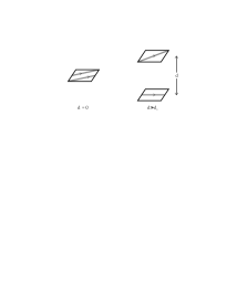
Figure 8: D-string configurations which are T-dual to a pair of separated 2-branes with a unit of flux (0-brane charge)

In fact, it turns out that the potential function $v(d)$ is constant for any $d$ greater than a critical distance $d_{c}$ [?]. Beyond this distance, the 0-brane and 2-brane have essentially no interaction classically. Below this distance, however, the solution where the flux is confined to a single 2-brane becomes unstable and the potential function drops continuously down to the value 1/2 at $d=0$. When quantum effects are included, for example by integrating out at one loop the off-diagonal terms, the potential is smoothed and the force between the objects becomes nonzero and attractive at arbitrary distance. These results agree perfectly with the full string calculation, which indicates that there is an attractive potential at all distances [?].

It is interesting to compare this analysis with a similar discussion by Douglas, Kabat, Pouliot and Shenker (DKPS) [?] of the potential between a pair of 1-branes carrying a single fundamental string charge. The situation they consider is dual to the 0-2 configuration we are discussing; however, because the quantization of electric field strength occurs only at the quantum level, the potential they calculate appears only when quantum effects are considered. The one-loop potential they calculate is smooth and gives a nonzero attractive force at all distances, as we expect from the one-loop calculation in the 0-2 case.

The fact that the force between the 0-brane and 2-brane is mostly localized within a finite distance $d_{c}$ provides a simple example of a general feature which is most clearly seen in brane-anti-brane interactions [?]. Namely, when two brane configurations are separately stable but can combine to form a lower energy configuration, at a distance analogous to $d_{c}$ a tachyonic instability appears in the system which indicates the existence of the lower energy configuration. A similar situation to the one we have described here occurs when two 2-branes are provided with 0-brane and anti-0-brane charges respectively. In this case when the 2-branes are brought sufficiently close a tachyonic instability appears which allows the 0-brane and anti-0-brane to annihilate. In the Yang-Mills language we are using here, these unstable modes can be explicitly constructed as degrees of freedom in the gauge field. Because of the nontrivial boundary conditions on the field, these degrees of freedom are described as theta functions which are sections of a nontrivial U(1) bundle on the torus. Using these theta functions, the tachyonic instabilities associated with brane-brane and brane-anti-brane forces can be precisely analyzed [?, ?].

5.2.3    Static 0-4 potential

Just as we placed a 0-brane on an auxiliary 2-brane to determine the form of the static 0-2 potential, we can place a 0-brane on a pair of auxiliary 4-branes to determine the static potential between a 0-brane and a 4-brane. Thus, we consider a set of 3 (uncompactified) 4-branes with a scalar field $X^{5}={\rm Diag}(d,d,0)$, with a $U(2)$ instanton living on the first two 4-branes. This configuration has a self-dual gauge field, so it is a BPS state in the moduli space of $U(3)$ instantons. Thus, the potential is independent of the distance $d$ even after quantum effects are considered and we see that there is no static potential between 0-branes and 4-branes. This is in agreement with the results from the full string calculation [?].

5.2.4    Static 0-6 and 0-8 potential

The static potential between a 0-brane and a 6-brane or an 8-brane is not as easy to understand from the point of view of gauge theory as in the 0-0, 0-2, and 0-4 cases, since there are no known 0-6 or 0-8 bound states. As mentioned in Section 5.1.4, however, a set of 4 or 8 0-branes can be smoothly distributed on the world-volume of 4 or 8 6-branes or 8-branes in a stable way after energy is added to the system. In the case of the 6-brane, this corresponds to the fact that there is a repulsive interaction between 0-branes and 6-branes (as determined by the string calculation), so that energy is needed to push them together from an infinite separation. Based on Yang-Mills theory alone, then, one might think that in the 0-8 case one would also get a repulsive force between the branes. There is an extra complication in this case, however, arising from interactions via R-R fields. In fact, the potential between separated 0-branes and 8-branes vanishes and such configurations preserve some supersymmetry. The 0-8 story has a number of subtleties, however. For example, as a 0-brane passes through an 8-brane, a (fundamental) string is created [?, ?, ?, ?]. This string produces a charge density on the 8-brane world-volume. The physics associated with this system is still a matter of some discussion.

5.2.5   0-brane scattering

We will now consider the interaction between a pair of moving 0-branes. The classical configuration space for a pair of 0-branes is the flat quotient space

$$\frac{({{R}}^{9})^{2}}{{{{Z}}}_{2}}.$$ (108)

As discussed in Section 5.2.1, this configuration space is protected by supersymmetry, so that all points in the space correspond to classical BPS states of the two 0-brane system. When the two 0-branes have a nonzero relative velocity, however, the supersymmetry of the system is broken and a velocity-dependent potential appears between the branes. The leading term in this potential can be determined by performing a one-loop calculation in the 0-brane quantum mechanics theory. We will now review this calculation briefly. The Yang-Mills calculation of the potential between two moving 0-branes was first carried out by Douglas, Kabat, Pouliot and Shenker [?]; many variations on this calculation have appeared in the literature over the last year or so, particularly in the context of Matrix theory. This calculation will be discussed further in Section 7.3.

To find the velocity-dependent potential at one-loop, we begin by considering a classical background solution for the two-particle system in which the two 0-branes are moving with relative velocity $v$ in the $X^{1}$ direction with an impact parameter of $b$ along the $X^{2}$ axis

$$X^{2}(t) = \left(\begin{array}[]{cc}b&0\\ 0&0\end{array}\right)$$ (111)

$$X^{1}(t) = \left(\begin{array}[]{cc}vt&0\\ 0&0\end{array}\right)$$ (114)

To calculate the effective potential between these 0-branes at one-loop order, we need to integrate out the off-diagonal fields. We can perform the calculation in background-field gauge, where we set

$$X^{a}=\langle X^{a}\rangle+\delta X^{a}$$ (115)

and where we add a background-field gauge fixing term

$$-\frac{1}{2R}\left(\dot{A}_{0}+i[\langle X^{a}\rangle,X^{a}]\right)^{2}$$ (116)

to the Lagrangian (2.3). We can calculate the one-loop potential by expanding the action to quadratic order in the off-diagonal fluctuations. In the quasi-static approximation, which is valid to leading order in the inverse separation [?], the potential is then simply given by the sum of the ground state energies of the corresponding harmonic oscillators. There are 10 (complex) bosonic oscillators, with frequencies

$$\omega_{b} = \sqrt{r^{2}}\;\;\;\;\;{\rm with\ multiplicity\ 8}$$

$$\omega_{b} = \sqrt{r^{2}\pm 2iv}\;\;\;\;\;{\rm with\ multiplicity\ 1\ each}.$$

where $r=\sqrt{b^{2}+v^{2}t^{2}}$ is the distance between the branes at time $t$. There are also 2 ghosts with frequencies

$$\omega_{g}=\sqrt{r^{2}},$$ (117)

and there are 16 fermions with frequencies

$$\omega_{f}=\sqrt{r^{2}\pm iv}\;\;\;\;\;{\rm with\ multiplicity\ 8\ each}.$$ (118)

The velocity-dependent potential is then given by

$$V=\sum_{b}\omega_{b}-2\omega_{g}-1/2\sum_{f}\omega_{f}.$$ (119)

For $v=0$ the frequencies clearly cancel and the potential vanishes. For nonzero $v$ we can expand each frequency in a power series in $1/r$. At the first three orders in $v/r^{2}$ the potential vanishes; the first nonvanishing term appears at fourth order, so that the potential between the 0-branes is given at leading order by

$$V(r)=\frac{-15v^{4}}{16\;r^{7}}.$$ (120)

As we will discuss in more detail in the following sections, it can be checked that this is in precise agreement with the corresponding potential in supergravity, including the multiplicative constant.

6 M(atrix) theory: The Conjecture

In the first four lectures we accumulated a fairly wide range of results which can be derived from the Yang-Mills description of D-branes. The last lecture (Sections 6, 7 and 8) contains an introduction to the Matrix theory conjecture, which states that the large $N$ limit of the Yang-Mills quantum mechanics of 0-branes contains a large portion of the physics of M-theory and string theory. As we shall see, much of the evidence for the Matrix theory conjecture is based on properties of the Yang-Mills description of D-branes which we have discussed in the context of type II string theory. The discussion given here of Matrix theory is fairly abbreviated and focuses on understanding how the objects and interactions of supergravity can be found in Matrix theory. The core of the material is based on the original lectures given in June of 1997; however, some more recent material is included which is particularly germane to the subject matter of the original lectures. Many important and interesting aspects of the theory are mentioned briefly, if at all. Other reviews which discuss some recent developments in more detail have been given by Banks [?] and by Susskind [?].

This section contains the statement of the Matrix theory conjecture as well as a brief review of some background material useful in understanding the statement of the conjecture, namely short reviews of M-theory and the infinite momentum frame. In Section 7 we discuss some of the evidence for Matrix theory, and in Section 8 we discuss some further directions in which this theory has been explored.

6.1 M-theory

The concept of M-theory has played a fairly central role in the development of the web of duality symmetries which relate the five string theories to each other and to supergravity [?, ?, ?, ?, ?]. M-theory is a conjectured eleven-dimensional theory whose low-energy limit corresponds to 11D supergravity [?]. Although there are difficulties with constructing a quantum version of 11D supergravity, it is a well-defined classical theory with the following field content:

$e^{a}_{I}$: a vielbein field (bosonic, with 44 components)
$\psi_{I}$: a Majorana fermion gravitino (fermionic, with 128 components)
$A_{IJK}$: a 3-form potential (bosonic, with 84 components).

In addition to being a local theory of gravity with an extra 3-form potential field, M-theory also contains extended objects. These consist of a two-dimensional supermembrane and a 5-brane.

One way of defining M-theory is as the strong coupling limit of the type IIA string. The IIA string theory is taken to be equivalent to M-theory compactified on a circle $S^{1}$, where the radius of compactification $R$ of the circle in direction 11 is related to the string coupling $g$ through $R=g^{2/3}l_{p}=gl_{s}$, where $l_{p}$ and $l_{s}=\sqrt{\alpha^{\prime}}$ are the M-theory Planck length and the string length respectively. The decompactification limit $R\rightarrow\infty$ corresponds then to the strong coupling limit of the IIA string theory. (Note that we will always take the eleven dimensions of M-theory to be labeled $0,1,\ldots,8,9,11$; capitalized roman indices $I,J,\ldots$ denote 11-dimensional indices).

Given this relationship between compactified M-theory and IIA string theory, a correspondence can be constructed between various objects in the two theories. For example, the Kaluza-Klein photon associated with the components $g_{\mu 11}$ of the 11D metric tensor can be associated with the R-R gauge field $A_{\mu}$ in IIA string theory. The only object which is charged under this R-R gauge field in IIA string theory is the 0-brane; thus, the 0-brane can be associated with a supergraviton with momentum $p_{11}$ in the compactified direction. The membrane and 5-brane of M-theory can be associated with different IIA objects depending on whether or not they are wrapped around the compactified direction; the correspondence between various M-theory and IIA objects is given in Table 1.

Table 1: Correspondence between objects in M-theory and IIA string theory

M-theory	IIA
KK photon ($g_{\mu 11}$)	RR gauge field $A_{\mu}$
supergraviton with $p_{11}=1/R$	0-brane
wrapped membrane	IIA string
unwrapped membrane	IIA D 2-brane
wrapped 5-brane	IIA D 4-brane
unwrapped 5-brane	IIA NS 5-brane

6.2 Infinite momentum frame

Roughly speaking, the infinite momentum frame (IMF) is a frame in which the physics has been heavily boosted in one particular direction. This frame has the advantage that it simplifies many aspects of relativistic quantum field theories [?]. To study a theory in the IMF, we begin by choosing a longitudinal direction; this will be $X^{11}$ in the case of M-theory. We then restrict attention to states which have very large values of momentum $p_{11}$ in the longitudinal direction. This is sometimes stated in the form that any system of interest should be heavily boosted in the longitudinal direction; however, this latter formulation leads to some subtleties, particularly when the longitudinal direction is compact. The basic idea of the IMF frame is that if we are interested in scattering amplitudes where the in-states and out-states have large values of $p_{11}$ then we can integrate out all the states with negative or vanishing $p_{11}$, giving a simplified theory. In general, intermediate states without large $p_{11}$ will indeed be highly suppressed. Degrees of freedom associated with zero-modes can cause complications, however [?].

One advantage of the IMF frame is that it turns a relativistic theory into one with a simpler, Galilean, invariance group. If a state has a large longitudinal momentum $p_{11}$ then to leading order in $1/p_{11}$ a Lorentz boost acts as a Galilean boost on the transverse momentum $p_{\bot}$ of the state

$$p_{\bot}\rightarrow p_{\bot}+p_{11}v_{\bot}.$$ (121)

A massless particle has an energy which is given to leading order in $1/p_{11}$ by a Galilean energy

$$E-p_{11}=\frac{p_{\bot}^{2}}{2p_{11}}$$ (122)

in the IMF. Thus, we see that the longitudinal momentum $p_{11}$ plays the role of the mass in the IMF Galilean theory.

If the longitudinal direction $X^{11}$ is compact with radius $R$, then longitudinal momentum is naturally quantized in units of $1/R$, so that $p_{11}=N/R$. Note that, as mentioned above, there are subtleties with boosting a compactified theory; in particular, a boost is not a symmetry of a Lorentz invariant theory which has been compactified in the direction of the boost, since after the boost the constant time surface becomes noncompact. By simply treating the IMF frame as a way of calculating interactions between states with large longitudinal momentum, however, this complication should not concern us particularly.

The description of a theory in the infinite momentum frame is closely related to the description of the theory given in light-front coordinates. In fact, for comparing Matrix theory to supergravity it is most convenient to use the language of discrete light-front quantization (DLCQ) [?]. In this framework a system is compactified in a lightlike dimension $x^{-}$ so that longitudinal momentum $p^{+}$ is quantized in units $N/R$, where we set

$$x^{\pm}=\frac{1}{\sqrt{2}}(x^{0}\pm x^{11}),\;\;\;\;\;x^{-}\equiv x^{-}+2\pi R$$ (123)

(note that the light-front metric has $\eta_{+-}=-1,\eta_{++}=\eta_{--}=0$). The DLCQ prescription gives a light-front description of a theory in the IMF when $N\rightarrow\infty$. Further discussion of DLCQ quantization in the context of Matrix theory can be found in [?, ?, ?, ?, ?].

6.3 The conjecture

The following conjecture was made by Banks, Fischler, Shenker and Susskind (BFSS) [?]:

M-theory in the IMF is exactly described by the $N\rightarrow\infty$ limit of 0-brane quantum mechanics

$${\cal L}=\frac{1}{2R}{\rm Tr}\;\left[\dot{X}^{a}\dot{X}_{a}+\sum_{a<b}[X^{a},X^{b}]^{2}+\theta^{T}(i\dot{\theta}-\Gamma_{a}[X^{a},\theta])\right]$$ (124)

where $N/R$ plays the role of the longitudinal momentum, and where $N/R$ and $R$ are both taken to $\infty$. Note that (124) is the same as (2.3) in units where $2\pi\alpha^{\prime}=1$, after replacing $g\sqrt{\alpha^{\prime}}=R$

Although we will continue to work in the string units in which (124) is expressed, in many references the Lagrangian is expressed in Planck units

$${\cal L}={\rm Tr}\;\left[\frac{1}{2R}\dot{X}^{a}\dot{X}_{a}+\frac{R}{8\pi^{2}}\sum_{a<b}[X^{a},X^{b}]^{2}+\frac{1}{4\pi}\theta^{T}(i\dot{\theta}-\frac{R}{2\pi}\;\Gamma_{a}[X^{a},\theta])\right].$$ (125)

The change of units can be carried out by simply replacing $\alpha^{\prime}\rightarrow l_{p}^{2}g^{-2/3}$ in (2.3) and setting $l_{p}=1$.

The original evidence for this conjecture included the following:

$\circ$ Only 0-branes carry $p_{11}$. Not only does this mean that states in M-theory with large $p_{11}$ are composed primarily of 0-branes, but this also fits naturally into the holographic principle espoused by ’t Hooft and Susskind [?, ?] which states that at large momentum string theory states can be described in terms of elementary partons which each take up a single Planck unit of transverse area. (Related ideas have also been discussed by Thorn [?].)

$\circ$ The 10D Super-Galilean invariance of (124).

$\circ$ The fact that graviton scattering amplitudes in 11D supergravity are correctly described by the scattering amplitude of 0-branes arising from the leading $v^{4}/r^{7}$ potential term.

$\circ$ The natural appearance of the supermembrane in the matrix quantum mechanics theory [?]. This connection between the low-energy theory of 0-branes and the light-front supermembrane theory was also pointed out by Townsend [?].

In the time since this conjecture was made, supporting evidence has continued to appear. In the following section, we will discuss some of this evidence.

6.4 Matrix compactification

Before discussing in detail the evidence for Matrix theory, let us discuss briefly the issue of compactifying the theory. Compactifying Matrix theory on a manifold $M$ would correspond to a compactification of M-theory on $M\times S^{1}$ where the $S^{1}$ is taken to a decompactified limit through $R\rightarrow\infty$. There are several ways in which BFSS suggested it might be possible to define a compactified version of Matrix theory.

The first approach to compactifying the theory would be to simply define Matrix theory on a manifold $M$ to be the large $N$ limit of the theory of $N$ 0-branes on $M$. For example, by using the equivalence discussed in Section 3.1 between the 0-brane theory on a torus and super Yang-Mills theory on the dual torus, this would define Matrix theory on the torus $T^{d}$ in terms of a $d$-dimensional super Yang-Mills theory. The torus can then be modded out by a finite group to get Matrix theory on an orbifold. So far 0-brane quantum mechanics is only very well understood on tori and orbifolds, however. There has been some progress made on curved manifolds, particularly on K3 and Calabi-Yau spaces [?, ?], however the situation is not as clear in these cases. Thus, this approach does not immediately lead to a candidate definition of Matrix theory compactified on an arbitrary manifold.

A second approach to compactifying Matrix theory involves taking superselection sectors of the theory which may correspond to different compactifications. For example, in the large $N$ limit we can take infinite matrices satisfying

$$UX^{a}U^{-1}=X^{a}+\delta^{a9}2\pi R_{9}{\hbox to0.0pt{1\hss}\hskip 1.6pt\hbox{1}}.$$ (126)

for some “translation” operator $U$ and radius $R_{9}$. This superselection sector of the theory corresponds to an $S^{1}$ compactification, since the matrices satisfying this relation can be interpreted in terms of the fields of $(1+1)$-D super Yang-Mills theory on the circle as in (35). In a similar way, it is easy to see that Matrix theory “contains” the SYM theory in all dimensions $d\leq 10$. It is an interesting open question whether there are other superselection sectors of the theory which naturally correspond to compactifications on non-toroidal spaces.

Both of these approaches to Matrix theory compactification give the same prescription for compactifying the theory on a torus. We will use this description of Matrix theory on a torus in terms of the super Yang-Mills theory on the dual torus in the following discussion. For compactification on tori of dimension $d>3$, however, additional features emerge which make the story more complicated. This issue will be discussed briefly in Section 8.2.

7 Matrix theory: Symmetries, Objects and Interactions

If the Matrix theory conjecture is correct, we would expect that all the symmetries of M-theory should correspond to symmetries of (124). Furthermore, it should be possible to find matrix constructions of all the objects we expect to see in the 11-dimensional supergravity theory which describes M-theory at low energies, and the interactions between these objects in Matrix theory should agree with the interactions between the corresponding supergravity objects. Most of the evidence to date for the Matrix theory conjecture consists of showing that some piece of this correspondence is correct. In this section we review some of this evidence, divided into the three categories mentioned. Recent arguments for the Matrix theory conjecture based on more general principles are discussed in Section 8.3.

7.1 Symmetries in Matrix theory

There are two important symmetries of M-theory which we would like to see reproduced in Matrix theory. First is the Lorentz symmetry of the theory. This is explicitly broken in the IMF; nonetheless, one would hope that a residual version of this symmetry would still be present. The second symmetry of M-theory which should be reproduced by Matrix theory is the group of duality symmetries of the theory. We now discuss these symmetries in turn.

7.1.1   Lorentz symmetry in Matrix theory

There is as of yet very little evidence for a residual Lorentz symmetry in Matrix theory. In fact, this is one of the directions in which the least progress has been made. Some evidence that the theory has Lorentz invariance at the classical level was given by de Wit, Marquard and Nicolai [?]. As stressed by BFSS, however, the quantum version of this argument is liable to be much more subtle. Other results relevant to the Lorentz symmetry of the theory include calculations of scattering with longitudinal momentum transfer which we discuss further below.

7.1.2   Duality in Matrix theory

In addition to Lorentz symmetry, M-theory has a set of duality symmetries which appear when the theory has been compactified on a $d$-dimensional torus. This group of “U-duality” symmetries increases in size and complexity as each additional dimension is compactified, as discussed in the lectures of Mukhi in this school. In this section we discuss the case $d=3$ in some detail. Compactification on tori of other dimensions is discussed briefly in Section 8.2.

After compactification on $T^{3}$, the U-duality group of M-theory is $SL(3,Z)\times SL(2,Z)$. This group is generated by two types of elementary symmetries. The $SL(3,Z)$ part of the U-duality group corresponds to the symmetry group of the moduli space of $T^{3}$ compactifications. Since this symmetry is simply related to the compactification space, it is a manifest symmetry of toroidally compactified Matrix theory. The $SL(2,Z)$ part of the U-duality group corresponds to a form of M-theory T-duality [?, ?]. Symmetries in this group can invert the volume of the compactification 3-torus, and are not manifest from the Matrix theory point of view. We will now discuss T-duality in M-theory and its realization in Matrix theory.

One simple way to understand T-duality in M-theory is through its relationship with IIA T-duality. If we compactify M-theory on a 3-torus in dimensions 8, 9 and 11, then we can draw the following commuting diagram of duality symmetries

Start with M-theory on the upper left. After compactification on dimension 11 (the vertical arrow) this becomes IIA on $T^{2}$. Two T-duality transformations give us another IIA theory on the dual of the original $T^{2}$. This corresponds to a new compactification of M-theory, so that by moving around the diagram we define an isomorphism of M-theory. This isomorphism is an element $T_{M}$ of the $SL(2,Z)$ T-duality group of M-theory.

A remarkable feature of this duality symmetry is that it acts on M-theory in a way which is symmetric in dimensions 8, 9 and 11. More precisely, after exchanging dimensions 8 and 9, the action of $T_{M}$ on the original compactification $T^{3}$ is to invert the volume of the torus through $T_{M}:V=R_{8}R_{9}R_{11}\leftrightarrow 1/V$. This can be verified directly by following the various coupling constants and radii around the diagram above.

It is interesting to consider the effects of the symmetry $T_{M}$ on the various string and membrane states in the theory. Momentum on the original $T^{3}$ can be identified with an element of the lattice dual to that defining the compactification torus. (i.e., for each compact direction $a$ on the torus there is a corresponding integer momentum $k_{a}$.) Similarly, a membrane which has been wrapped around some 2-cycle on $T^{3}$ can be identified with a vector on the dual lattice which is perpendicular to the membrane. M-theory T-duality exchanges these two dual vectors, swapping membrane wrapping number with string momentum in the compact directions. We can easily check this in various special cases by following the T-duality symmetry through the above diagram. For example, if we begin with an M-theory membrane wrapped in directions 9 and 11, after projection into IIA this becomes a string wrapped on dimension 9. Two IIA T-dualities take this into a string with momentum in dimension 9 and no winding. Exchanging dimensions 8 and 9 turns this into momentum in dimension 8. This lifts back into momentum in dimension 8 in M-theory, which is a vector orthogonal to the original 9-11 membrane. The reader can check as an exercise that an 8-9 membrane in M-theory is mapped into a state with 11-momentum in a similar fashion.

Now that we have discussed M-theory T-duality in some detail, we can ask how this symmetry is realized in Matrix theory. We would expect that if Matrix theory is compactified on a 3-torus, say in dimensions 7, 8 and 9, then the theory should have an $SL(2,Z)$ group of self-duality symmetries corresponding to the group of M-theory T-dualities. From the discussion of compactification in Section 6.4, we expect that Matrix theory on $T^{3}$ should correspond to ${\cal N}=4$ super Yang-Mills theory on the dual $\hat{T}^{3}$. In fact, this theory does have a nontrivial $SL(2,Z)$ self-duality symmetry: the S-duality symmetry discussed in Section 3.2. This is precisely the duality symmetry which implements the Matrix theory version of M-theory T-duality [?, ?].

As evidence for this identification of ${\cal N}=4$ super Yang-Mills S-duality with Matrix theory T-duality, we can consider the following observations: First, as discussed in Section 3.1.2, the Yang-Mills coupling constant for Matrix theory on $T^{3}$ is given by

$$\tau=\frac{i}{g_{{\rm YM}}^{2}}\sim iV_{789}.$$ (127)

Under one element of the SYM S-duality group this coupling constant is inverted through $\tau\rightarrow-1/\tau$; this corresponds to the inversion of the volume of the torus which we expect from the element $T_{M}$ of the M-theory T-duality group. Second, SYM S-duality exchanges electric and magnetic fluxes. We have identified membranes in Matrix theory with magnetic flux in the corresponding SYM theory

$${\rm Tr}\;[X^{a},X^{b}]\sim\int iB^{ab}$$ (128)

and momentum in Matrix theory with electric flux through

$${\rm Tr}\;\Pi^{a}={\rm Tr}\;\dot{X^{a}}\sim\int{\rm Tr}\;\dot{A_{a}}=\int{\rm Tr}\;E^{a}.$$ (129)

The exchange of these quantities corresponds precisely to the exchange of membrane winding and momentum expected of M-theory T-duality.

Thus, although S-duality in ${\cal N}=4$ super Yang-Mills has not yet been definitively proven, we have strong evidence that Matrix theory has the expected T-duality symmetry of M-theory, and that it can be expressed precisely in terms of this more widely accepted field theory duality symmetry. Combining the $SL(2,Z)$ of SYM S-duality with the manifest $SL(3,Z)$ symmetry of the 3-torus we find that Matrix theory has the full U-duality group expected from M-theory compactified on a 3-torus.

7.2 Matrix theory objects

We will now discuss evidence that Matrix theory contains most or all of the objects which we expect to see in the 11-dimensional supergravity theory which is the low-energy limit of M-theory.

7.2.1   Supergravitons

Let us first discuss the appearance of supergravitons in Matrix theory. Since 0-branes are the carriers of longitudinal momentum, we would expect a supergraviton with longitudinal momentum $N/R$ to correspond to a bound state of $N$ 0-branes. From the fact that Matrix theory has 16 supersymmetries, we know that threshold bound states of 0-branes must live in a 256-dimensional representation of the supersymmetry algebra. This corresponds precisely to the number of Kaluza-Klein modes of the supergraviton arising from the graviton, 3-form, and gravitino (256 = 44 + 84 + 128). It has been shown that these bound states exist, at least for $N$ prime [?, ?, ?].

One remarkable feature of Matrix theory which is worth emphasizing at this point is that second quantization is automatic in Matrix theory. That is, not only does Matrix theory naturally contain a set of states corresponding to single gravitons, it actually has a Hilbert space containing states with arbitrary numbers of separated gravitons. The point is that in the large $N$ limit we can have matrices which break up into an arbitrary number of blocks. For example, a state with the schematic form

$$\left(\begin{array}[]{cccc}M_{1}^{a}&0&0&\ddots\\ 0&M_{2}^{a}&\ddots&0\\ 0&\ddots&\ddots&0\\ \ddots&0&0&M_{k}^{a}\end{array}\right)$$ (130)

could describe a state of $k$ supergravitons, where the matrices $M_{i}$ are $N_{i}\times N_{i}$ matrices and the longitudinal momentum of the $i$th graviton is $p_{+}=N_{i}/R$. A matrix of this form, of course, corresponds to a classical Matrix theory configuration. A quantum state describing multiple separated gravitons would be described by a wavefunction which would approximate the tensor product of a number of bound state wavefunctions as the separations between the gravitons are taken to be very large.

7.2.2   Supermembranes

We now discuss the appearance of the supermembrane in Matrix theory. It was realized many years ago that there is a remarkable connection between matrix quantum mechanics and the light-front supermembrane [?, ?, ?, ?]. From the point of view that has been taken in these notes, the easiest way to see that the supermembrane must appear in Matrix theory is to note that the (unwrapped) supermembrane corresponds to the 2-brane of type IIA string theory. As discussed in Section 4.6, when the theory is compactified on a 2-torus of area $A$, a 2-brane can be built from 0-branes by constructing a 0-brane configuration with

$${\rm Tr}\;[X^{1},X^{2}]=\frac{iA}{2\pi}.$$ (131)

The energy of this configuration is

$$E=-\frac{1}{2R}{\rm Tr}\;[X^{1},X^{2}]^{2}=\frac{A^{2}}{8\pi^{2}RN}=\frac{A^{2}}{32\pi^{4}\alpha^{\prime 2}RN},$$ (132)

where factors of $2\pi\alpha^{\prime}$ have been restored in the final expression. This corresponds to the second term in an expansion in $1/N$ of the Born-Infeld energy for a system of $N$ 0-branes and a single 2-brane

$$E_{{\rm BI}}=\sqrt{(N\tau_{0})^{2}+(A\tau_{2})^{2}}=N\tau_{0}+\frac{A^{2}\tau_{2}^{2}}{2N\tau_{0}}+\cdots.$$ (133)

Rewritten in Planck units the energy is

$$E=\frac{A^{2}R}{32\pi^{4}N}$$ (134)

which is precisely the light-front energy $E=(T_{2}A)^{2}/2p^{+}$ for an M-theory membrane with area $A$, tension $T_{2}=1/(2\pi)^{2}$ and longitudinal momentum $p^{+}$.

To describe an infinite flat supermembrane in the noncompact theory, we can consider a pair of infinite matrices $X^{1},X^{2}$ satisfying

$$[X^{1},X^{2}]=\frac{i}{2\pi\rho}{\hbox to0.0pt{1\hss}\hskip 1.6pt\hbox{1}}$$ (135)

For example, these matrices could be taken to be proportional to the operators $q,p=-i\;d/dq$ acting on wave functions in one dimension [?]. Comparing to (131) we see that $\rho\sim N/A$ corresponds to the density of 0-branes (longitudinal momentum) on the membrane. Note that (135) cannot be satisfied by any finite dimensional matrices, but has solutions only in the large $N$ limit.

In addition to flat membranes which are either infinite or wrapped around a compact direction, it is desirable to have a Matrix theory description of finite-size compact membranes moving in a noncompact space. In fact, precisely such configurations were described in the work of de Wit, Hoppe and Nicolai almost a decade ago [?]. These authors studied the supermembrane theory in eleven dimensions in light-front coordinates. In light-front gauge, the supermembrane theory has a residual invariance under the group of area-preserving diffeomorphisms on the world-volume. This group can be identified as a large $N$ limit of $SU(N)$. This leads to a discretization of the supermembrane theory which gives precisely the 0-brane quantum mechanics theory. The key ingredient in the derivation of this result is the construction of an explicit correspondence between functions on the membrane and matrices in $U(N)$ [?, ?]. In the case of a membrane of spherical topology, this correspondence is particularly simple; functions on the 2-sphere which are expressed in terms of polynomials in the euclidean coordinates $x_{1},x_{2},x_{3}$ are described in Matrix theory by the equivalent symmetrized polynomials in the generators $J_{1},J_{2},J_{3}$ of the $N$-dimensional representation of $SU(2)$. As a simple example, we can consider the matrix representation of a symmetric 2-sphere. A rotationally invariant 2-sphere of radius $r$ can be embedded in the first three transverse directions of space through

$$X_{a}=\frac{2r}{N}J_{a},\;\;\;\;\;a\in\{1,2,3\}.$$ (136)

Even at finite $N$ this matrix configuration has a number of geometrical properties which are associated with a smooth 2-sphere [?]. For example, the matrices $X_{a}$ satisfy

$$X_{1}^{2}+X_{2}^{2}+X_{3}^{2}=r^{2}{\hbox to0.0pt{1\hss}\hskip 1.6pt\hbox{1}}+{\cal O}(1/N^{2})$$ (137)

so that in a noncommutative sense the component 0-branes are constrained to lie on the 2-sphere. This construction of the Matrix theory spherical membrane is closely related to the “fuzzy” 2-sphere which appears in mathematical work on noncommutative geometry [?, ?]. Toroidal Matrix theory membranes are similarly related to the fuzzy torus [?].

7.2.3   Longitudinal 5-branes

We now discuss 5-branes in Matrix theory. There are two ways in which the M-theory 5-brane can appear as an object in Matrix theory. On the one hand, it can be wrapped around the longitudinal direction, in which case it appears as a 4-brane in Matrix theory. On the other hand, it can be unwrapped in the longitudinal direction in which case it should appear as a true (NS) 5-brane in Matrix theory. We will discuss both cases, but we begin with the longitudinal 5-brane (L5-brane).

Longitudinal 5-branes in Matrix theory were first discussed by Berkooz and Douglas [?]. They included these branes as backgrounds for the 0-brane quantum mechanics theory by including hypermultiplets in the theory corresponding to 0-4 strings. In this work the L5-branes did not appear as dynamical objects described in terms of matrix variables. The authors showed, however, that a membrane which is moved around the L5-brane in the background will pick up a Berry’s phase which corresponds with that expected from the effects of the 3-form field in supergravity.

A description of L5-branes in terms of Matrix theory variables can be given in a fashion directly analogous to the above discussion of the membrane [?]. If we compactify on a $T^{4}$ of volume $V$ then as discussed in Section 4.6 a flat 4-brane wrapped around the torus can be constructed from a set of matrices satisfying

$${\rm Tr}\;\epsilon_{abcd}X^{a}X^{b}X^{c}X^{d}=\frac{V}{2\pi^{2}}$$ (138)

Taking the large volume limit of the torus, a construction of a noncompact 4-brane with longitudinal momentum density $N/V=\rho$ can be given in terms of infinite matrices satisfying

$$\epsilon_{abcd}X^{a}X^{b}X^{c}X^{d}=\frac{1}{2\pi^{2}\rho}{\hbox to0.0pt{1\hss}\hskip 1.6pt\hbox{1}}.$$ (139)

There are a number of ways of constructing a configuration of this type. One can construct a “stack of 2-branes” solution with 2-brane charge as well as 4-brane charge [?]. It is also possible to construct a configuration with no 2-brane charge by identifying $X^{a}$ with the components of the covariant derivative operator for an instanton on $S^{4}$

$$X^{a}=i\partial^{a}+A_{a}.$$ (140)

This construction is known as the Banks-Casher instanton [?].

Just as for the membrane, it is possible to construct a matrix configuration corresponding to an L5-brane which has the transverse geometry of a symmetric 4-sphere [?]. A spherical configuration corresponding to $n$ superimposed L5-brane spheres with radius $r$ is defined through

$$X_{a}=\frac{r}{n}G_{a},\;\;\;\;\;a\in\{1,\ldots,5\}.$$ (141)

where $G_{a}$ are the generators of the $n$-fold symmetric tensor product representation of the five four-dimensional gamma matrices $\Gamma_{a}$. Although these configurations have the geometrical and physical properties expected of $n$ coincident L5-brane spheres, they also have a number of surprising characteristics. These configurations can only be defined for $N$ of the form

$$N=\frac{(n+1)(n+2)(n+3)}{6}.$$ (142)

Furthermore, unlike the case of the membrane 2-sphere where arbitrary fluctuations can be described by symmetrized polynomials in the generators $J_{a}$, it seems that no similar approach correctly describes fluctuations around the symmetric 4-sphere configuration. This Matrix 4-sphere is closely related to the fuzzy 4-sphere which has been discussed in the context of noncommutative geometry [?].

7.2.4   Transverse 5-branes

A systematic way of understanding the membrane and 5-brane charges in Matrix theory arises from considering the supersymmetry algebra of the theory. Schematically, the 11-dimensional supersymmetry algebra takes the form

$$\{Q,Q\}\sim P^{I}+Z^{I_{1}I_{2}}+Z^{I_{1}\ldots I_{5}}$$ (143)

where the central terms correspond to 2-brane and 5-brane charges. The supersymmetry algebra of Matrix theory was explicitly computed by Banks, Seiberg and Shenker [?]. Similar calculations had been performed previously [?, ?]; however, in these earlier analyses terms such as ${\rm Tr}\;[X^{a},X^{b}]$ and ${\rm Tr}\;X^{[a}X^{b}X^{c}X^{d]}$ were dropped since they vanish for finite $N$. The full supersymmetry algebra of the theory takes the form

$$\{Q,Q\}\sim P^{I}+z^{a}+z^{ab}+z^{abcd}.$$ (144)

The charge

$$z^{ab}\sim{\rm Tr}\;[X^{a},X^{b}]$$ (145)

corresponds to membrane charge. The charge

$$z^{abcd}\sim{\rm Tr}\;X^{[a}X^{b}X^{c}X^{d]}$$ (146)

corresponds to longitudinal 5-brane charge, as we have just discussed. The charge

$$z^{a}\sim{\rm Tr}\;\{P^{b},[X^{a},X^{b}]\}$$ (147)

corresponds to longitudinal membranes (strings). This can be understood easily in a dual Yang-Mills picture, where this charge corresponds to the Poynting vector $F^{ab}E^{b}$; as usual, momentum is the dual of string winding number.

Nowhere in this analysis of brane charges do we see any sign of a charge corresponding to transverse 5-branes. As we will see in the next section, there is also no sign of such a charge in the general expression for the leading long-range gravitational interaction between two matrix objects [?]. It was argued by Banks, Seiberg and Shenker that in fact transverse 5-branes cannot exist in the IMF since they are Dirichlet objects for the M-theory membrane [?]. Nonetheless, there is an argument [?] that a T5-brane can be constructed implicitly using the super Yang-Mills S-duality of Matrix theory on $T^{3}$. We now review this argument briefly.

Let us compactify M-theory on dimensions 7, 8 and 9. We now place an infinite membrane along dimensions 5 and 6. Performing M-theory T-duality on dimensions 7, 8 and 9 has the effect of taking the membrane to a 5-brane wrapped around dimensions 5-9, as can be seen in the following commuting diagram

Thus, to construct a T5-brane in Matrix theory we must begin with the theory compactified on $T^{3}$ in dimensions 7-9, with a Yang-Mills configuration having scalar fields satisfying

$$[X^{5},X^{6}]\sim i{\hbox to0.0pt{1\hss}\hskip 1.6pt\hbox{1}}$$ (148)

Performing SYM S-duality on this state should give a transverse 5-brane. There are a number of puzzling subtleties regarding this construction, however. First, we have no explicit representation of S-duality in 4D SYM, so we cannot construct the T5-brane state explicitly. Second, there is a confusing issue about how the large $N$ limit must be taken. In order to construct a configuration like (148) we must take the large $N$ limit before performing the S-duality transformation. It is unclear how SYM S-duality behaves in the large $N$ limit. Finally, if this state truly exists, a good reason needs to be found why the corresponding charge does not appear in the supersymmetry algebra or in the leading term in the long-distance potential. It is possible that this charge may be nonlocal, and vanishes for a reason analogous to the vanishing of the L5-brane and membrane charges at finite $N$.

7.3 Interactions in Matrix theory

7.3.1   The leading $1/r^{7}$ potential

We now turn our attention to the interactions between the objects of Matrix theory. We discussed in Section 5.2.5 the calculation of the velocity-dependent effective potential (120) between a pair of 0-branes in super Yang-Mills quantum mechanics. This potential was found as the result of a one-loop calculation in the Yang-Mills theory. As pointed out by BFSS [?], this potential corresponds precisely with the leading long-range supergravity potential between a pair of gravitons with longitudinal momentum $1/R$ in light-front coordinates. An explicit calculation shows that the leading term in the long-range supergravity potential between a pair of pointlike objects with momenta $\hat{p}^{I}$ and $\tilde{p}^{I}$ due to the exchange of a single graviton with no longitudinal momentum is (in string units)

$$V_{\rm gravity}=-{15\over 4}\,{R^{4}\over r^{7}}\left[\left(\hat{p}\cdot\tilde{p}\right)^{2}-{1\over 9}\hat{p}^{2}\tilde{p}^{2}\right].$$ (149)

Taking one of the Matrix theory 0-branes to be at rest and the other to have transverse velocity $v^{a}$, we have

$$\hat{p}^{+}=\frac{1}{R}\;\;\;\;\; \hat{p}^{a}=0\;\;\;\;\;\;\;\;\;\;\;\;\;\hat{p}^{-}=0$$ (150)

$$\tilde{p}^{+}=\frac{1}{R}\;\;\;\;\; \tilde{p}^{a}=\frac{v^{a}}{R}\;\;\;\;\;\;\;\;\;\;\tilde{p}^{-}=\tilde{p}^{2}_{\perp}/2\tilde{p}^{+}=\frac{v^{2}}{2R}$$

Inserting these momenta into (149) gives

$$V_{{\rm gravity}}=-\frac{15v^{4}}{16\;r^{7}}$$ (151)

in exact agreement with (120). This exact correspondence carries through for states with longitudinal momentum $p^{+}=N/R$. The gravitational potential in this case is simply multiplied by the product $\hat{N}\tilde{N}$. The same factor enters the Yang-Mills calculation because this is the multiplicity of string states stretching between the two collections of 0-branes, assuming that each of the two states is described by a localized bound state of $N$ 0-branes.

In the last year or so, the one-loop potential has been calculated for a variety of Matrix theory objects [?, ?, ?, ?, ?, ?, ?, ?, ?, ?, ?, ?, ?, ?]. In all cases this potential was found to agree at leading order with the expected leading long-distance potential from supergravity. A general proof of this result was given by Kabat and the author in [?]; we will now describe briefly the analysis in the general case. Given a pair of classical Matrix theory objects described by matrices $\hat{X}$ and $\tilde{X}$ of sizes $\hat{N}\times\hat{N}$ and $\tilde{N}\times\tilde{N}$ respectively, the one-loop potential between these objects can be calculated in the quasi-static appropriation by taking a background configuration

$$\langle X^{a}\rangle=\left(\begin{array}[]{cc}\hat{X}^{a}&0\\ 0&\tilde{X}^{a}\end{array}\right).$$ (152)

Summing the frequencies of the string oscillators associated with the bosons, fermions and ghosts in the off-diagonal matrix blocks as in (119) gives the one-loop potential between the two objects. If the centers of mass of the two objects are separated by a distance $r$ which is large compared to the sizes of the objects then this potential can be expanded in powers of $1/r$. The leading term is of the form $F^{4}/r^{7}$ where $F$ can be a term of the form $\dot{X}$ or $[X,X]$ [?, ?]. Decomposing the general expression for this term into functions of $\hat{X}$ and $\tilde{X}$, and grouping terms by their Lorentz structure it can be shown [?] that the leading term in the Matrix theory potential between an arbitrary pair of separated objects is given by

$$V_{\rm matrix}=V_{\rm gravity}+V_{\rm electric}+V_{\rm magnetic}$$ (153)

where

$$V_{\rm gravity} = -{15R^{2}\over 4r^{7}}\left({\hat{\cal T}}^{IJ}\tilde{{\cal T}}_{IJ}-{1\over 9}{\hat{\cal T}}^{I}{}_{I}\tilde{{\cal T}}^{J}{}_{J}\right)$$

$$V_{\rm electric} = -{45R^{2}\over r^{7}}{\hat{\cal J}}^{IJK}{\tilde{\cal J}}_{IJK}$$ (154)

$$V_{\rm magnetic} = -{45R^{2}\over r^{7}}\hat{{\cal M}}^{+-ijkl}\tilde{{\cal M}}^{-+ijkl}$$

and where we define the following quantities: ${\cal T}^{IJ}$ is a symmetric tensor with components

$${\cal T}^{--} = {1\over R}\;{\rm STr}\,\left(\frac{1}{4}\dot{X}^{a}\dot{X}^{a}\dot{X}^{b}\dot{X}^{b}+{1\over 4}\dot{X}^{a}\dot{X}^{a}F^{bc}F^{bc}+\dot{X}^{a}\dot{X}^{b}F^{ac}F^{cb}\right.$$

$$\qquad\qquad\left.+{1\over 4}F^{ab}F^{bc}F^{cd}F^{da}-\frac{1}{16}F^{ab}F^{ab}F^{cd}F^{cd}\right)$$

$${\cal T}^{-a} = {1\over R}\;{\rm STr}\,\left(\frac{1}{2}\dot{X}^{a}\dot{X}^{b}\dot{X}^{b}+{1\over 4}\dot{X}^{a}F^{bc}F^{bc}+F^{ab}F^{bc}\dot{X}^{c}\right)$$

$${\cal T}^{+-} = {1\over R}\;{\rm STr}\,\left(\frac{1}{2}\dot{X}^{a}\dot{X}^{a}+{1\over 4}F^{ab}F^{ab}\right)$$ (155)

$${\cal T}^{ab} = {1\over R}\;{\rm STr}\,\left(\dot{X}^{a}\dot{X}^{b}+F^{ac}F^{cb}\right)$$

$${\cal T}^{+a} = {1\over R}\;{\rm STr}\,\dot{X}^{a}$$

$${\cal T}^{++} = {1\over R}\;{\rm STr}\,{\hbox to0.0pt{1\hss}\hskip 1.6pt\hbox{1}}={N\over R}$$

${\cal J}^{IJK}$ is a totally antisymmetric tensor with components

$${\cal J}^{-ab} = {1\over 6R}{\rm STr}\,\left(\dot{X}^{a}\dot{X}^{c}F^{cb}-\dot{X}^{b}\dot{X}^{c}F^{ca}-\frac{1}{2}\dot{X}^{c}\dot{X}^{c}F^{ab}\right.$$

$$\qquad\qquad\left.+{1\over 4}F^{ab}F^{cd}F^{cd}+F^{ac}F^{cd}F^{db}\right)$$

$${\cal J}^{+-a} = {1\over 6R}{\rm STr}\,\left(F^{ab}\dot{X}^{b}\right)$$ (156)

$${\cal J}^{abc} = -{1\over 6R}{\rm STr}\,\left(\dot{X}^{a}F^{bc}+\dot{X}^{b}F^{ca}+\dot{X}^{c}F^{ab}\right)$$

$${\cal J}^{+ab} = -{1\over 6R}{\rm STr}\,F^{ab}$$

and ${\cal M}^{IJKLMN}$ is a totally antisymmetric tensor with

$${\cal M}^{+-abcd}={1\over 12R}{\rm STr}\,\left(F^{ab}F^{cd}+F^{ac}F^{db}+F^{ad}F^{bc}\right)\,.$$ (157)

We have defined $F_{ab}=-i[X_{a},X_{b}]$. The trace ${\rm STr}\,$ is defined to be the trace symmetrized over all possible orderings of the factors $\dot{X}$ and $F$. Tensors $\hat{{\cal T}}^{IJ},\tilde{{\cal T}}^{IJ}$, etc. are defined through (155-157) as functions of $\hat{X}$ and $\tilde{X}$. Note that the only components of ${\cal M}$ which appear in (154) are those defined in (157); there is no expression known for other components of this tensor.

The general form of the Matrix theory potential (153) can be compared with the leading long-distance potential in 11D supergravity between an arbitrary pair of objects. In supergravity this potential arises from the exchange of a single particle, which must be either a graviton or 3-form quantum. In light-front coordinates the propagator for a quantum carrying no longitudinal momentum carries a factor of $\delta(\hat{x}^{+}-\tilde{x}^{+})$ [?]. Thus, we expect the light-front supergravity potential to be instantaneous in light-front time. An explicit calculation of this potential shows that the leading term is precisely given by (153) where ${\cal T}$, ${\cal J}$ and ${\cal M}$ are the integrated stress tensor, membrane current and 5-brane current in supergravity. Thus, if we use (155), (156) and (157) as definitions of the integrated stress tensor and currents in Matrix theory, we see that there is an exact correspondence between the leading term in the one-loop Matrix theory potential and the leading term in the supergravity potential for an arbitrary pair of objects.

7.3.2   Further aspects of Matrix theory interactions

Although the correspondence between Matrix theory and supergravity interactions has been demonstrated in general at order $1/r^{7}$, the current understanding of subleading terms is much less developed. There are a number of ways in which subleading terms appear in the Matrix theory potential. A systematic analysis of the structure of the subleading terms in the graviton scattering amplitude was carried out by Becker, Becker, Polchinski and Tseytlin (BBPT) [?] and has also been considered by Susskind. Generally, at $n$th loop order, there are terms in the potential of order $v^{4+2k}/r^{4+3n+4k}$ for all values of $k$. For more general Matrix theory objects, the structure is similar, with $F$ playing the role of $v$; however, there are also dependencies on the fields $X$ so that the full expansion is of the form

$$V=\sum_{n,k,l}V_{nkl}\frac{F^{4+2k}X^{l}}{r^{4+l+3n+4k}}$$ (158)

where $n$ indicates the loop order at which a given term arises. Generally, the contraction of the indices of $F$ and $X$ can be carried out in many inequivalent ways; the coefficient $V_{nkl}$ therefore is shorthand for many independent coefficients at each order, corresponding to all possible contractions. We will now discuss some of the features of this loop expansion which are currently understood. Note that our discussion focuses on interactions between purely bosonic states. When fermions are included there can be additional effects such as spin effects; it has been found that these effects seem to be captured accurately by Matrix theory also, at least at leading order [?, ?, ?].

If we consider only the terms in the one-loop expansion which contain four powers of $F$, the expansion reduces to a sum of terms of the form $F^{4}X^{l}/r^{7+l}$. This set of terms was analyzed in [?, ?], where it was shown that these terms can be described in terms of interactions between higher moments of the Matrix theory stress tensor (155), membrane current (156) and L5-brane current (157). These interactions correspond precisely to the higher-order terms expected from supergravity for the interaction between two extended objects due to single graviton or 3-form exchange. It seems reasonable to conclude that the role of the factors $X^{l}/r^{l}$ will in general be to incorporate higher moments of extended objects; thus, to understand the remaining terms in (158) it will suffice to restrict attention to the terms with $l=0$, which are the only ones contributing in the case of graviton scattering.

One set of terms of particular interest are the terms of the form $F^{4}/r^{4+3n}$. If such terms existed with nonvanishing coefficients beyond one-loop order they would renormalize the $v^{4}$ interaction term which already agrees at one-loop order with supergravity. It was conjectured by BFSS that no such renormalization occurs. Becker and Becker have performed the calculation explicitly for graviton scattering at two-loop order and shown that the term of order $v^{4}/r^{10}$ vanishes identically [?]. This supports the hypothesis that all remaining $v^{4}$ terms vanish; however, this has not been shown at higher order. It has also been suggested that the $v^{4}$ terms may in fact be renormalized at higher loop order since analogous renormalizations occur in three-dimensional theories [?]. These terms may also be affected by processes with longitudinal momentum transfer, which we discuss briefly below.

The next several terms which contribute at two loops have also been calculated for graviton scattering. It was shown by BBPT [?] that the term of order $v^{6}/r^{14}$ is also in agreement with the potential expected from classical supergravity. This term corresponds to a general relativistic correction to the lowest order term in the potential. All the terms in the Matrix theory potential of the form $v^{4+2m}/r^{7m}$ carry integral powers of the gravitational constant when expressed in Planck units. It is believed that these terms should reproduce classical supergravity to all orders. Although none of these terms have been calculated precisely beyond two loops, it has been argued [?, ?, ?, ?] that the general form of these terms should correspond with higher order terms in the non-abelian Born-Infeld action. Although these terms cannot be determined uniquely by this ansatz, in certain cases exact expressions for the supergravity interactions are of the Born-Infeld form, and are in agreement with this conjecture.

At each loop order there are terms which contribute at higher order in $1/r$ than the terms which are expected to correspond with classical supergravity. It is believed that these terms represent quantum gravity corrections. There has been some discussion of this question in the literature [?, ?, ?, ?, ?, ?], but as yet there does not seem to be a detailed understanding of this issue.

The loop expansion in Matrix theory which we have been discussing only describes processes in which no longitudinal momentum is exchanged. Clearly, for a full understanding of interactions in Matrix theory it will be necessary to include processes with longitudinal momentum transfer. Some progress has been made in this direction. Polchinski and Pouliot have calculated the scattering amplitude for two 2-branes for processes in which a 0-brane is transferred from one 2-brane to the other [?]. In the Yang-Mills picture the incoming and outgoing configurations in this calculation are described in terms of a $U(2)$ gauge theory with a scalar field taking a VEV which separates the branes, as discussed in Section 5.2.2. The transfer of a 0-brane corresponds to an instanton-like process where a unit of flux is transferred from one brane to the other. The results of this calculation are in agreement with expectations from supergravity. This result suggests that processes involving longitudinal momentum transfer may be correctly described in Matrix theory. Note, however, that the Polchinski-Pouliot calculation is not precisely a calculation of membrane scattering with longitudinal momentum transfer in Matrix theory since it is carried out in the 2-brane gauge theory language. In the T-dual Matrix theory picture the process in question corresponds to a scattering of 0-branes in a toroidally compactified space-time with the transfer of membrane charge. This process was studied further by Dorey, Khoze and Mattis [?] and was related to graviton scattering by Banks, Fischler, Seiberg and Susskind [?].

8 Matrix theory: Further Developments

In the last year there has been a veritable explosion of Matrix theory related papers. In this section we describe briefly a few of the interesting directions in which this work has gone. There are a number of important and interesting developments which we do not discuss here at all. In particular, nothing is said in these notes about the recent developments on Matrix theory black holes or light-front 5-brane theories. We also do not discuss Matrix theory compactification on orbifolds. Although we do give a brief description of the DVV formulation of Matrix string theory, there are many other interesting formulations of string theory in the matrix language, such as heterotic Matrix strings, which we do not cover here. Another particularly interesting set of developments involves the compactification of Matrix theory on higher dimensional tori. Aside from a few brief comments, this topic is not covered. Some of these topics are covered in more detail in the reviews [?, ?].

8.1 Matrix string theory

An interesting feature of Matrix theory is that with a few minor modifications it can be used to give a nonperturbative definition of string theory. A number of approaches have been taken to Matrix string theory [?, ?, ?, ?]. In this section we review briefly a few aspects of the Matrix string theory approach due to Dijkgraaf, Verlinde and Verlinde (DVV) [?, ?].

If we consider Matrix theory compactified in dimension 9 on a circle $S^{1}$, we have a super Yang-Mills theory in $(1+1)$-D on the dual circle $\hat{S}^{1}$. In the BFSS formulation of Matrix theory, this corresponds to M-theory compactified on a 2-torus. If we now think of dimension 9 rather than dimension 11 as the dimension which has been compactified to get a IIA theory, then we see that this super Yang-Mills theory should provide a light-front description of type IIA string theory. Because we are now interpreting dimension 9 as the dimension of M-theory compactification, the fundamental objects which carry momentum $p^{+}$ are no longer 0-branes, but rather strings with longitudinal momentum. Thus, it is natural to interpret $N/R$ in this super Yang-Mills theory as the longitudinal string momentum. It was argued by Dijkgraaf, Verlinde and Verlinde that in fact this gives a natural corollary to the Matrix theory conjecture, namely that 2D super Yang-Mills in the large $N$ limit should correspond to light-front IIA string theory.

To examine this form of the conjecture in more detail, let us begin by considering the Matrix theory Hamiltonian (working in Planck units and dropping factors of order unity as in [?])

$$H=R_{11}{\rm Tr}\;\left[\Pi_{a}\Pi_{a}-[X^{a},X^{b}]^{2}+\theta^{T}\gamma_{a}[X^{a},\theta]\right]\ .$$ (159)

After compactification on $R_{9}$ we identify $X^{9}\rightarrow R^{9}D_{\sigma}$, $\Pi_{9}\rightarrow R_{9}\dot{A}_{9}\sim E_{9}/R_{9}$, where $\sigma\in[0,2\pi]$ is the coordinate on the dual circle. With these identifications, and using $g\sim R_{9}^{3/2}$, the Hamiltonian was rewritten by DVV in the form

$$H = \frac{R_{11}}{2\pi}\int d\sigma\;{\rm Tr}\;\left[\Pi_{a}\Pi_{a}+(D_{\sigma}X^{a})^{2}+\theta^{T}D_{\sigma}\theta\right.$$ (160)

$$\hskip 72.26999pt\left.+\frac{1}{g^{2}}\left(E^{2}-[X^{a},X^{b}]^{2}\right)+\frac{1}{g}\theta^{T}\gamma_{a}[X^{a},\theta]\right]\ .$$

This is essentially the form of the Green-Schwarz light-front string Hamiltonian, with the modification that the fields are now $N\times N$ matrices which do not necessarily commute. This means that the theory automatically contains multi-string objects living in a second quantized Hilbert space. Furthermore, it is possible to construct extended string theory objects in terms of the noncommuting matrix variables, by a simple translation from the original Matrix theory language. We reproduce in Table 2 a table of the extended objects in this Matrix string theory. The objects are listed in terms of their interpretations in M-theory, as well as their interpretations in Matrix string theory and associated charges in Matrix string theory. Charges are given only up to an overall constant.

Table 2: Objects and their charges in Matrix string theory

M-theory	Matrix string object	Matrix string charge
$p_{11}$	$p^{+}$	$N$
$p_{9}$	D$0$	$E$
$p_{a}$	$p_{a}$	$\Pi_{a}$
M${}_{a9}\;\;$ ($a-9$ membrane)	$w_{a}\;\;$(wound string)	$D_{\sigma}X^{a}$
M11 9	$w_{+}$	$\Pi_{a}(D_{\sigma}X^{a})\;\;(E\times B)$
Mab	D$2_{ab}$	$[X^{a},X^{b}]$
Ma 11	D$2_{a+}$	$ED_{\sigma}X^{a}+\Pi_{b}[X^{a},X^{b}]$
$5_{abc+9}$	D$4_{abc+}$	$D^{[9}X^{a}X^{b}X^{c]}$
$5_{abcd+}$	NS$5_{abcd+}$	$X^{[a}X^{b}X^{c}X^{d]}$

To verify each of the entries in this table it suffices to consider a Matrix theory object with its known charge, and to rewrite that object and charge in terms of the Yang-Mills description after the “9-11 flip” corresponding to interpreting dimension 9 as the M-theory compactification direction. For example, consider an M-theory membrane wrapped in dimensions 8-9. In BFSS Matrix theory this is a membrane with charge $[X^{8},X^{9}]$. In Matrix string theory we take $X^{9}\rightarrow D_{9}$ so that the charge becomes $D_{9}X^{8}$. Since dimension 9 is the M-theory compactification direction, this corresponds to a string wrapped around dimension 8. Note that the only objects missing in this table are those corresponding to the T5-brane in BFSS Matrix theory. These correspond to a 4-brane or 5-brane wrapped in transverse directions in Matrix string theory.

One particularly nice feature of the DVV approach to Matrix string theory is the way in which the individual string bits carrying a single unit of longitudinal momentum combine to form long strings. As the string coupling becomes small $g\rightarrow 0$, the coefficient of the term $[X^{a},X^{b}]^{2}$ in the Hamiltonian becomes very large. This forces the matrices to become simultaneously diagonalizable. Because the string configuration is defined over $S^{1}$, however, the matrix configuration need not be periodic in $\sigma$. The matrices $X^{a}(0)$ and $X^{a}(2\pi)$ can be related by an arbitrary permutation. The lengths of the cycles of this permutation determine the numbers of string bits which combine into long strings whose longitudinal momentum $N/R_{11}$ can become large in the large $N$ limit. As the coupling becomes very small, the theory therefore essentially becomes a sigma model on $({{R}}^{8})^{N}/S^{N}$. The twisted sectors of this theory correspond precisely to the sectors where the string bits are combined in different permutations. In this picture, string interactions appear as vertex operators in the conformal field theory arising as the infrared limit of the sigma model theory. It is not apparent, however, how such interactions are related to the Yang-Mills description of the theory. It would be nice to have a more direct understanding of this relationship.

Some discussion is given in the original DVV papers of the structure of D-branes in Matrix string theory. This is another direction in which it would be interesting to develop the theory in further detail. For example, DVV suggest that a 0-brane corresponds to a single string bit which does not become part of an extended string in the large $N$ limit. It would be nice if there were a natural way in which the known properties of 0-branes could be derived from this point of view. Clearly, there is more to be said about the relationship between Matrix string theory and other formulations of light-front string theory.

8.2 Compactification of more than three dimensions

As discussed in Section 6.4, Matrix theory compactified on a torus of dimension $d\leq 3$ is described in terms of super Yang-Mills theory on the dual torus. Compactification on $T^{3}$ was described in section 7.1.2. Compactification of the theory on $T^{2}$ was discussed by Sethi and Susskind [?]. They pointed out that as the $T^{2}$ shrinks, a new dimension appears whose quantized momentum modes correspond to magnetic flux on the $T^{2}$. In the limit where the area of the torus goes to 0, an $O(8)$ symmetry appears. This corresponds with the fact that IIB string theory appears as a limit of M-theory on a small 2-torus [?, ?]. When more than three dimensions are toroidally compactified, the theory undergoes even more remarkable transformations [?]. For example, consider compactifying the theory on $T^{4}$. The manifest symmetry group of this theory is $SL(4,Z)$. The expected U-duality group of M-theory compactified on $T^{4}$ is $SL(5,Z)$, however. It was pointed out by Rozali [?] that the U-duality group can be completed by interpreting instantons on $T^{4}$ as momentum states in a fifth compact dimension. This means that Matrix theory on $T^{4}$ is most naturally described in terms of a (5 + 1)-dimensional theory with a chiral $(2,0)$ supersymmetry. This $(2,0)$ theory is an unusual theory with 16 supersymmetries [?] which appears to play a crucial role in a wide variety of properties of M-theory and 5-branes.

Compactification on tori of higher dimensions than four continues to lead to more complicated situations, particularly in the case of $T^{6}$. A significant amount of literature has been produced on this subject, to which the reader is referred to further details (see for example [?, ?, ?, ?] and references therein). Despite the complexity of $T^{6}$ compactification, however, it was recently suggested by Kachru, Lawrence and Silverstein [?] that compactification of Matrix theory on a more general Calabi-Yau 3-fold might actually lead to a simpler theory than that resulting from compactification on $T^{6}$.

8.3 Proofs and counterexamples

Since the time when these lectures were given, there has been a great deal of debate about whether the Matrix theory conjecture is truly correct to all orders in perturbation theory, and if so, why. The results of this debate are still uncertain, and a full discussion of the issues involved will not be given here. We will only briefly review a few of the points in the discussion.

It was suggested by Susskind [?] that there might be a sense in which the Matrix theory conjecture holds even at finite $N$. This extended version of the conjecture would relate finite $N$ Matrix theory with the finite $N$ discrete light-cone quantization of M-theory. An argument has been given by Seiberg [?] which seems to indicate that this correspondence is correct, and related discussions have been given by Sen [?] and de Alwis [?]. Seiberg’s approach even seems to apply to compactification of Matrix theory on an arbitrary manifold, although the details of this argument have not been made precise.

However, there are also a number of pieces of evidence that the correspondence between Matrix theory and supergravity breaks down in certain contexts. Attempts to formulate Matrix theory on curved spaces seem to lead to discrepancies between the leading terms in the Matrix theory and supergravity interaction potentials [?, ?]. Higher-loop effects on orbifolds also seem to give rise to discrepancies [?, ?] (further comments on this issue appear in [?]). Even in flat space, it seems that Matrix theory may have problems in reproducing supergravity: Recently Dine and Rajaraman considered 3-graviton scattering in Matrix theory [?], and argued that there are certain diagrams in supergravity with nonzero amplitudes which simply cannot be reproduced at any order in Matrix theory. When considering interactions between extended objects, it also seems that Matrix theory may diverge from supergravity in unusual ways; although the one-loop interaction between any two objects must agree with supergravity if the components of the source tensors are defined as in Section 7.3.2, the components of the stress tensor for extended objects are defined so that the equivalence principle seems to break down at finite $N$ [?].

Thus, we seem to be faced with a contradiction: on the one hand proofs that even at finite $N$ Matrix theory is a correct description of DLCQ M-theory, on the other hand evidence that Matrix theory does not agree with results one would expect from supergravity. Some recent papers have addressed this puzzle [?, ?, ?, ?]; however, a complete resolution of the situation will certainly take some time. It may be that to resolve these issues it will be necessary to understand the large $N$ limit of Matrix theory in a more precise fashion. It may also be that detailed aspects of the bound state wave functions of gravitons will play a role in resolving these contradictions.

9 Conclusions

We have seen that a remarkable number of interesting properties of D-branes can be understood from the point of view of the low-energy super Yang-Mills description. Super Yang-Mills theory contains information about all the known duality symmetries of type II string theory and M-theory. We can construct higher- and lower-dimensional branes of various types directly within the super Yang-Mills theory for branes of a particular dimension. Super Yang-Mills theory even seems to know about supergravity. From super Yang-Mills theory we have some suggestion of how to generalize our notions of geometry to include noncommutative spaces such as those of Connes [?]. All this is certainly an indication that super Yang-Mills theory is a much richer theory than it has usually been given credit for. Whether it will truly reproduce all of the physics of string theory, let alone the standard model, however, remains to be seen. To this author, it seems that there is still some fundamental principle lacking. In particular, for Matrix theory to leave the IMF or light-front gauge, it is necessary to introduce anti-0-branes. These are virtually the only objects which cannot be constructed from 0-branes as some kind of generalized fluxes. As has been suggested by a number of authors, it seems that we need some more fundamental structure in which all the objects of the theory, even 0-branes and anti-0-branes, appear as some generalized type of fluxes or as composites of some underlying medium. Because of the way in which quantum mechanics and geometrical constraints often seem to be related through dualities, it easy to imagine that whatever fundamental principles we are currently lacking will necessitate a rather substantial reworking of our concepts of quantum mechanics and field theory themselves.

References

References

- [1] T. Banks, W. Fischler, S. Shenker, and L. Susskind, “M Theory as a Matrix Model: A Conjecture,” hep-th/9610043.
- [2] J. Polchinski, S. Chaudhuri, and C. V. Johnson, “Notes on D-Branes,” hep-th/9602052.
- [3] J. Polchinski, “TASI Lectures on D-branes,” hep-th/9611050.
- [4] M. B. Green, J. H. Schwarz and E. Witten, Superstring theory (Cambridge University Press, Cambridge, 1987).
- [5] J. Polchinski, “Dirichlet-Branes and Ramond-Ramond Charges,” Phys. Rev. Lett. 75 (1995) 4724, hep-th/9510017.
- [6] J. Dai, R. G. Leigh, and J. Polchinski, Mod. Phys. Lett. A4 (1989) 2073.
- [7] R. G. Leigh, Mod. Phys. Lett. A4 (1989) 2767.
- [8] E. Witten, “Bound States of Strings and p-Branes,” Nucl. Phys. B460 (1996) 335, hep-th/9510135.
- [9] M. Claudson and M. Halpern, Nucl. Phys. B250 (1985) 689.
- [10] R. Flume, Ann. of Phys. 164 (1985) 189.
- [11] M. Baake, P. Reinicke and V. Rittenberg, J. Math. Phys. 26 (1985) 1070.
- [12] U. Danielsson, G. Ferretti, and B. Sundborg, Int. J. Mod. Phys. A11 (1996) 5463-5478, hep-th/9603081.
- [13] D. Kabat and P. Pouliot, “A Comment on Zero-Brane Quantum Mechanics,” Phys. Rev. Lett. 77 (1996) 1004-1007, hep-th/9603127.
- [14] M. R. Douglas, D. Kabat, P. Pouliot, and S. Shenker, “D-Branes and Short Distances in String Theory,” hep-th/9608024.
- [15] C. M. Hull and P. K. Townsend, Nucl. Phys. B438 (1995) 109, hep-th/9410167.
- [16] E. Witten, “String Theory Dynamics in Various Dimensions,” Nucl. Phys. B443 (1995) 85, hep-th/9503124.
- [17] W. Taylor, “D-brane Field Theory on Compact Spaces,” Phys. Lett. B394 (1997) 283, hep-th/9611042.
- [18] O. J. Ganor, S. Ramgoolam and W. Taylor, “Branes, Fluxes and Duality in M(atrix)-Theory,” hep-th/9611202.
- [19] M. R. Douglas and G. Moore, “D-branes, Quivers, and ALE Instantons,” hep-th/9603167.
- [20] E. Gimon and J. Polchinski, Phys. Rev. D54 (1996) 1667.
- [21] C. V. Johnson and R. C. Myers, “Aspects of Type IIB Theory on ALE Spaces,” hep-th/9610140.
- [22] A. Connes, M. R. Douglas and A. Schwarz, “Noncommutative geometry and Matrix theory: compactification on tori,” hep-th/9711162.
- [23] M. R. Douglas and C. Hull, “D-branes and the noncommutative torus,” hep-th/9711165.
- [24] P.-M. Ho, Y.-Y. Wu and Y.-S. Wu, “Towards a noncommutative approach to matrix compactification,” hep-th/9712201.
- [25] J. H. Schwarz, Phys. Lett. B360 (1995) 13, Erratum-ibid. B364 (1995) 252, hep-th/9508143.
- [26] C. Montonen and D. Olive, Phys. Lett. B72 (1977) 117.
- [27] E. Witten and D. Olive, “Supersymmetry Algebras that Include Topological Charges,” Phys. Lett. B78 (1978) 97.
- [28] H. Osborn, Phys. Lett. B83 (1979) 321.
- [29] F. Ferrari, Nucl. Phys. B501 (1997) 53-96, hep-th/9702166.
- [30] M. Bershadsky, C. Vafa and V. Sadov, Nucl. Phys. B463 (1996) 420, hep-th/9511222.
- [31] M. B. Green, J. A. Harvey and G. Moore, Class. Quant. Grav. 14 (1997) 47-52, hep-th/9605033.
- [32] Y.-K. E. Cheung and Z. Yin, Nucl. Phys. B517, 69-91 (1998), hep-th/9710206.
- [33] R. Minasian and G. Moore, “K theory and Ramond-Ramond charge,” hep-th/9710230.
- [34] T. Eguchi, P. Gilkey and A. Hanson, “Gravitation, Gauge Theories and Differential Geometry,” Phys. Rep. 66 (1980) 213.
- [35] E. Witten, “Small Instantons in String Theory,” Nucl. Phys. B460 (1996) 541, hep-th/9511030.
- [36] M. R. Douglas, “Branes within Branes,” hep-th/9512077.
- [37] M. Li, Nucl. Phys. B460 (1996) 351, hep-th/9510161.
- [38] C. Bachas, “D-Brane Dynamics,” Phys. Lett. B374 (1996) 37-42, hep-th/9511043.
- [39] E. Bergshoeff, M. de Roo, M. B. Green, G. Papadopoulos and P. K. Townsend, Nucl. Phys. B470 (1996) 113, hep-th/9601150.
- [40] E. Alvarez, J. L. F. Barbon and J. Borlaf, Nucl. Phys. B479 (1996) 218-242, hep-th/9603089.
- [41] G. ’t Hooft, Nucl. Phys. B153 (1979) 141.
- [42] A. Hashimoto and W. Taylor, “Fluctuation Spectra of Tilted and Intersecting D-branes from the Born-Infeld Action,” hep-th/9703217.
- [43] Z. Guralnik and S. Ramgoolam, Nucl. Phys. B499 (1996) 241-252, hep-th/9702099.
- [44] P. van Baal, Nucl. Phys. B49 (Proc.Suppl.) (1996) 238-249, hep-lat/9508019.
- [45] M. Berkooz, M. R. Douglas, and R. Leigh, “Branes Intersecting at Angles,” Nucl. Phys. B480 (1996) 265, hep-th/9606139.
- [46] T. Banks, N. Seiberg, and S. Shenker, “Branes from Matrices,” hep-th/9612157.
- [47] K. Stelle, “Lectures on supergravity -branes,” hep-th/9701088.
- [48] A. Sen, Phys. Rev. D54 (1996) 2964-2967, hep-th/9510229.
- [49] A. Sen, Phys. Rev. D53 (1996) 2874-2894, hep-th/9511026.
- [50] A. A. Tseytlin, “On Non-Abelian Generalisation of Born-Infeld Action in String Theory,” hep-th/9701125.
- [51] P. K. Townsend, Phys. Lett. B373 (1996) 68, hep-th/9512062.
- [52] Z. Guralnik and S. Ramgoolam, “From 0-branes to Torons,” hep-th/9708089.
- [53] M. Green and M. Gutperle, “Light-Cone Supersymmetry and D-branes,” Nucl. Phys. B476 (1996) 484, hep-th/9604091.
- [54] V. Balasubramanian and R. Leigh, Phys. Rev. D55 (1997) 6415-6422, hep-th/9611165.
- [55] C. Vafa, “Instantons on D-branes,” Nucl. Phys. B463 (1996) 435, hep-th/9512078.
- [56] M. R. Douglas, “Gauge Fields and D-Branes,” RU-96-24, hep-th/9604198.
- [57] S. K. Donaldson and P. B. Kronheimer, The geometry of four-manifolds (Clarendon Press, Oxford, 1990).
- [58] C. Vafa, “Gas of D-Branes and Hagedorn Density of BPS States,” Nucl. Phys. B463 (1996) 415-419, hep-th/9511088.
- [59] J. A. Harvey and G. Moore, “On the algebras of BPS states,” hep-th/9609017.
- [60] H. Nakajima, Tokyo lectures on Hilbert schemes of points on surfaces.
- [61] W. Taylor, “Adhering 0-branes to 6-branes and 8-branes,” hep-th/9705116.
- [62] R. Khuri, T. Ortin, “A Non–Supersymmetric Dyonic Extreme Reissner–Nordstrom Black Hole,” Phys. Lett. B373 (1996) 56, hep-th/9512178.
- [63] H. Sheinblatt, “Statistical Entropy of an Extremal Black Hole with 0- and 6-Brane Charge,” hep-th/9705054.
- [64] S. Sethi and M. Stern, “D-brane Bound States Redux,” hep-th/9705046.
- [65] B. Simon, Ann. Phys. 146 (1983) 209.
- [66] G. Lifschytz, “Comparing D-branes to Black-branes,” hep-th/9604156.
- [67] P. van Baal, Nucl. Phys. B47 (Proc.Suppl.) (1996) 326-329, hep-lat/9508019.
- [68] T. Banks and L. Susskind, “Brane-antibrane forces”, hep-th/9511194.
- [69] E. Gava, K. S. Narain and M. H. Sarmadi, “On the Bound States of and Branes,” hep-th/9704006.
- [70] A. Hanany and E. Witten, “Type IIB Superstrings, BPS Monopoles, and Three-Dimensional Gauge Dynamics,” hep-th/9611230.
- [71] C. Bachas, M. R. Douglas and M. Green, “Anomalous Creation of Branes,” hep-th/9705074.
- [72] U. Danielsson, G. Ferretti and I. Klebanov, “Creation of Fundamental Strings by Crossing D-branes,” hep-th/9705084.
- [73] O. Bergman, M. R. Gaberdiel and G. Lifschytz, “Branes, Orientifolds and the Creation of Elementary Strings,” hep-th/9705130.
- [74] Ø. Tafjord and V. Periwal, “Finite-time amplitudes in Matrix theory,” hep-th/ 9711046.
- [75] T. Banks, “Matrix Theory,” hep-th/9710231.
- [76] D. Bigatti and L. Susskind, “Review of matrix theory,” hep-th/9712072.
- [77] M. J. Duff, J. T. Liu and R. Minasian, Nucl. Phys. B452 (1995) 261, hep-th/9506126.
- [78] J. H. Schwarz , Phys. Lett. 367 (1996) 97, hep-th/9510086.
- [79] P. Horava and E. Witten, Nucl. Phys. B460 (1996) 506, hep-th/9510209.
- [80] E. Cremmer, B. Julia and J. Scherk, Phys. Lett. B76 (1978) 409.
- [81] Kogut and L. Susskind, Phys. Rep. 8 (1973) 75-172.
- [82] S. Hellerman and J. Polchinski, “Compactification in the Lightlike Limit,” hep-th/9711037.
- [83] L. Susskind, “Another Conjecture about M(atrix) Theory,” hep-th/9704080.
- [84] A. Sen, “D0 Branes on and Matrix Theory,” hep-th/9709220.
- [85] N. Seiberg, “Why is the Matrix Model Correct?,” Phys. Rev. Lett. 79 (1997) 3577, hep-th/9710009.
- [86] D. Bigatti and L. Susskind, “A note on discrete light cone quantization,” hep-th/9711063.
- [87] G. ’t Hooft, in Proc. Salamfest ’93 (1993), gr-qc/9310026.
- [88] L. Susskind, J. Math. Phys. 36 (1995) 6377-6396, hep-th/9409089.
- [89] C. B. Thorn, in Proc. of Sakharov Conf. on Physics, Moscow (1991) 447-454, hep-th/9405069.
- [90] B. de Wit, J. Hoppe and H. Nicolai, Nucl. Phys. B305 [FS 23] (1988) 545.
- [91] M. R. Douglas, H. Ooguri and S. Shenker, “Issues in M(atrix) Theory Compactification,” hep-th/9702203.
- [92] M. R. Douglas and H. Ooguri, “Why Matrix Theory is Hard,” hep-th/9710178.
- [93] B. de Wit, V. Marquard and H. Nicolai, Comm. Math. Phys. 128 (1990) 39.
- [94] O. Aharony, “String theory dualities from M-theory,” hep-th/9604103.
- [95] L. Susskind, “T-duality in M(atrix)-theory and S-duality in Field Theory,” hep-th/9611164.
- [96] P. Yi, Nucl. Phys. B505 (1997) 307, hep-th/9704098.
- [97] M. Porrati and A. Rozenberg, “Bound states at threshold in supersymmetric quantum mechanics,” hep-th/9708119.
- [98] J. Goldstone, unpublished.
- [99] J. Hoppe, MIT Ph.D. thesis (1982); J. Hoppe, in proc. Int. Workshop on Constraint’s Theory and Relativistic Dynamics; eds. G. Longhi and L. Lusanna (World Scientific, 1987).
- [100] E. A. Bergshoeff, E. Sezgin and Y. Tanii, Nucl. Phys. B298 (1988) 187.
- [101] D. Kabat and W. Taylor, “Spherical membranes in Matrix theory,” hep-th/9711078.
- [102] J. Madore, J. Math. Phys. 32 (1991) 332.
- [103] J. Madore, Non-commutative geometry and applications (Cambridge, 1995).
- [104] M. Berkooz and M. R. Douglas, “Five-branes in M(atrix) Theory,” hep-th/9610236.
- [105] T. Banks and A. Casher, Nucl. Phys. B167 (1980) 215.
- [106] J. Castelino, S. Lee and W. Taylor, “Longitudinal 5-branes as 4-spheres in Matrix theory,” hep-th/9712105.
- [107] H. Grosse, C. Klimčík, P. Prešnajder , “On finite 4D quantum field theory in non-commutative geometry,” hep-th/9602115.
- [108] D. Kabat and W. Taylor, “Linearized supergravity from Matrix theory,” hep-th/9712185.
- [109] O. Aharony and M. Berkooz, “Membrane Dynamics in M(atrix) Theory,” hep-th/9611215.
- [110] G. Lifschytz and S. Mathur, “Supersymmetry and Membrane Interactions in M(atrix) Theory,” hep-th/9612087.
- [111] G. Lifschytz, “Four-brane and Six-brane Interactions in M(atrix) Theory,” hep-th/9612223.
- [112] D. Berenstein and R. Corrado, “M(atrix) Theory in Various Dimensions,” hep-th/9702108.
- [113] G. Lifschytz, “A Note on the Transverse Five-Brane in M(atrix) Theory,” hep-th/9703201.
- [114] I. Chepelev and A. Tseytlin, “Long-distance interactions of D-brane bound states and longitudinal 5-brane in M(atrix) theory,” hep-th/9704127.
- [115] J. Maldacena, “Probing near extremal black holes with D-branes,” hep-th/9705053.
- [116] E. Keski-Vakkuri and P. Kraus, “Notes on Branes in Matrix Theory,” hep-th/9706196.
- [117] R. Gopakumar and S. Ramgoolam, “Scattering of zero branes off elementary strings in Matrix theory,” hep-th/9708022.
- [118] I. Chepelev and A. Tseytlin, “Long-distance interactions of branes: correspondence between supergravity and super Yang-Mills descriptions,” hep-th/9709087.
- [119] J. Maldacena, “Branes Probing Black Holes,” hep-th/9709099.
- [120] E. Keski-Vakkuri and P. Kraus, “Born-Infeld actions from Matrix theory,” hep-th/9709122.
- [121] R. R. Metsaev and A. A. Tseytlin, Nucl. Phys. B298 (1988) 109.
- [122] K. Becker, M. Becker, J. Polchinski, and A. Tseytlin, “Higher Order Graviton Scattering in M(atrix) Theory,” hep-th/9706072.
- [123] J. A. Harvey, “Spin dependence of D0-brane interactions,” hep-th/9706039.
- [124] J. Morales, C. Scrucca and M. Serone, “A note on supersymmetric D-brane dynamics,” hep-th/9709063.
- [125] P. Kraus, “Spin-Orbit interaction from Matrix theory,” hep-th/9709199.
- [126] W. Taylor and M. Van Raamsdonk, “Angular momentum and long-range gravitational interactions in Matrix theory,” hep-th/9712159.
- [127] K. Becker and M. Becker, “A Two-Loop Test of M(atrix) Theory,” hep-th/9705091.
- [128] M. Dine and N. Seiberg, “Comments on higher derivative operators in some SUSY field theories,” hep-th/9705057.
- [129] V. Balasubramanian, R. Gopakumar and F. Larsen, “Gauge theory, geometry and the large N limit,” hep-th/9712077.
- [130] I. Chepelev and A. Tseytlin, “On Membrane Interaction in Matrix Theory,” hep-th/9801120.
- [131] L. Susskind, Talk at Strings ’97.
- [132] P. Berglund and D. Minic, “A note on effective Lagrangians in matrix-theory,” hep-th/9708063.
- [133] M. Serone, “A Comment on the Coupling in M(atrix) Theory,” hep-th/9711031.
- [134] E. Keski-Vakkuri and P. Kraus, “Short distance contributions to graviton-graviton scattering: Matrix theory versus supergravity,” hep-th/9712013.
- [135] K. Becker and M. Becker, “On Graviton Scattering Amplitudes in M-theory,” hep-th/9712238.
- [136] J. Polchinski and P. Pouliot, “Membrane Scattering with M-Momentum Transfer,” hep-th/9704029.
- [137] N. Dorey, V. V. Khoze and M. P. Mattis, Nucl. Phys. B502 (1997) 94-106, hep-th/9704197.
- [138] T. Banks, W. Fischler, N. Seiberg, and L. Susskind, Phys. Lett. B408 (1997) 111-116, hep-th/9610043.
- [139] N. Ishibashi, H. Kawai, Y. Kitazawa and A. Tsuchiya, “A Large-N Reduced Model as Superstring,” hep-th/9612115.
- [140] L. Motl, “Proposals on nonperturbative superstring interactions,” hep-th/9701025.
- [141] T. Banks and N. Seiberg, “Strings from Matrices,” hep-th/9702187.
- [142] R. Dijkgraaf, E. Verlinde, H. Verlinde, Nucl. Phys. B500 (1997) 43-61, hep-th/9703030.
- [143] R. Dijkgraaf, E. Verlinde, H. Verlinde, “Notes on Matrix and Micro Strings,” hep-th/9709107.
- [144] S. Sethi and L. Susskind, Phys. Lett. B400 (1997) 265-268, hep-th/9702101.
- [145] P. Aspinwall, “Some relationships between dualities in string theory,” hep-th/9508154.
- [146] W. Fischler, E. Halyo, A. Rajaraman and L. Susskind, “The Incredible Shrinking Torus,” hep-th/9703102.
- [147] M. Rozali, “Matrix theory and U-duality in seven dimensions,” hep-th/9702136.
- [148] N. Seiberg, “Notes on Theories with 16 Supercharges,” hep-th/9705117.
- [149] M. Berkooz, “String Dualities from Matrix Theory: a Summary,” hep-th/9712012.
- [150] O. J. Ganor and S. Sethi, “New perspectives on Yang-Mills theories with sixteen supersymmetries,” hep-th/9712071.
- [151] S. Kachru, A. Lawrence and E. Silverstein, “On the Matrix Description of Calabi-Yau Compactifications,” hep-th/9712223.
- [152] S. de Alwis, “Matrix Models and String World Sheet Duality,” hep-th/9710219.
- [153] O. J. Ganor, R. Gopakumar and S. Ramgoolam, “Higher loop effects in M(atrix) orbifolds,” hep-th/9705188.
- [154] J. R. David, A. Dhar and G. Mandal, Phys. Lett. B415, 135-143 (1997), hep-th/9707132
- [155] M. Dine and A. Rajaraman, “Multigraviton Scattering in the Matrix Model,” hep-th/9710174.
- [156] A. Bilal, “A comment on compactification of M-theory on an (almost) lightlike circle,” hep-th/9801047.
- [157] A. Connes, Noncommutative geometry (Academic Press, New York, 1994).