Abstract

We discuss the construction of the physical configuration space for Yang-Mills quantum mechanics and Yang-Mills theory on a cylinder. We explicitly eliminate the redundant degrees of freedom by either fixing a gauge or introducing gauge invariant variables. Both methods are shown to be equivalent if the Gribov problem is treated properly and the necessary boundary identifications on the Gribov horizon are performed. In addition, we analyze the significance of non-generic configurations and clarify the relation between the Gribov problem and coordinate singularities.

1 Introduction

Gauge field theories are at the heart of the standard model of the fundamental interactions. The weak coupling phase of the model is rather well understood in terms of standard perturbation theory. This is sufficient for the electro-weak theory where for the physically relevant scales weak and electromagnetic couplings are small. For the strong interactions, however, the situation is different. At small momentum transfer, or large distances, the associated gauge theory of color $SU(3)$, quantum chromodynamics (QCD), is in the strong coupling phase and perturbation theory no longer works. One therefore has to develop nonperturbative techniques, the most elaborate one at the moment being lattice gauge theory [1, 2, 3].

An alternative approach, based on Bjorken’s idea of the femto-universe [4] has been initiated by Lüscher [5] and was later elaborated by van Baal and collaborators [6]. In this approach, one formulates QCD in a finite volume which in a first step is kept sufficiently small so that, due to asymptotic freedom, perturbation theory is still valid. Upon enlarging the volume, nonperturbative effects come into play, however, as is believed, in a controllable manner. Technically, one uses a Hamiltonian formulation of QCD or, neglecting quarks, pure Yang-Mills theory in the Coulomb gauge [7]. The way the nonperturbative effects show up is conceptually simple [8]. For small volumes, the wave functionals behave essentially as those in QED, i.e. they are concentrated around the classical vacuum. For larger volumes, the effective coupling increases, the wave functionals start to spread out in configuration space and become sensitive to its boundaries and nontrivial geometry [9]. It is therefore crucial for the understanding of these effects to learn as much as possible about the structure of the configuration space. Let us illuminate this reasoning with an example from quantum mechanics. For a particle in an infinitely deep square well of size $d$ there is a gap between the ground and first excited state of order $1/d^{2}$. Obviously, the existence of the finite energy gap is directly related to the finite volume of the configuration space. Similar arguments have been given by Feynman to explain the origin of the mass gap for Yang-Mills theory in 2+1 dimensions [10] and are currently being re-investigated [11].

Let us discuss the case of non-Abelian gauge theories [12] in more detail. The configuration space $\mathcal{A}$ of pure Yang-Mills theory is given in terms of the gauge fields (“configurations”) $A(x)$, which under the action of the gauge group $\mathcal{G}$ transform as

$${}^{U}{\!A}=\,U^{-1}A\,U+i\>U^{-1}\mathrm{d}U\quad\text{with}\quad U\in{\mathcal{G}}\;.$$ (1)

The set of all gauge equivalent points ${}^{U}{\!A}$ of a given configuration $A$ constitutes the orbit of $A$. Gauge invariance requires physical quantities to take the same value for every configuration ${}^{U}{\!A}$ on the orbit of $A$. In this sense, the description of gauge theories in terms of the potentials $A$ is somewhat uneconomic as there is a huge redundancy associated with these variables. One way to see this is the infinite volume factor they contribute to the path integral measure. It is therefore desirable to find the set of all gauge inequivalent configurations, i.e. the space of gauge orbits

$$\mathcal{M}:=\mathcal{A}/\mathcal{G}\;,$$ (2)

which we will refer to as the physical configuration space $\mathcal{M}$. The interesting question, of course, is, how to actually find $\mathcal{M}$. A first hint can be obtained from (2), which can naively be “solved” for $\mathcal{A}$ yielding

$$\mathcal{A}\sim\mathcal{M}\times\mathcal{G}\;.$$ (3)

Though at this point it is unclear in which sense this identity really holds, it nevertheless suggests that the large configuration space $\mathcal{A}$ of gauge potentials should be decomposed into gauge invariant quantities from $\mathcal{M}$ and gauge variant ones parameterizing group elements $U\in\mathcal{G}$. The decomposition indicated in (3) can explicitly be achieved using the transformation law (1): parameterize the group elements $U[\varphi]$ with an appropriate collection of angle variables $\varphi$ such that $U[\varphi\!=\!0]=1\!\!\!\>\text{l}$, then pick a representative $\tilde{A}$ on any orbit and rewrite (1) as

$$A[\tilde{A},\varphi]\,:=\,^{U}{\!\tilde{A}}=U^{-1}[\varphi]\,\tilde{A}\>U[\varphi]+i\>U^{-1}[\varphi]\>\mathrm{d}U[\varphi]\;.$$ (4)

Thus, any gauge potential $A$ carries an (implicit) label $\varphi$ which determines the position of $A$ on its orbit, in particular $A=\tilde{A}$ for $\varphi=0$. The identity (4) defines a map $(\tilde{A},\varphi)\mapsto A$ which provides (at least locally) the decomposition of an arbitrary configuration $A$ into a gauge invariant representative $\tilde{A}$ and the gauge variant angles $\varphi$. In general, this map will be a transformation from the cartesian coordinates $A$ to curvilinear coordinates $(\tilde{A},\varphi)$ [7, 13].

Usually, the representative $\tilde{A}$ of the orbit is chosen via gauge fixing, i.e. by defining functionals $\chi$ on $\mathcal{A}$ such that

$$\chi[\tilde{A}\,]=0\;,$$ (5)

This defines a hypersurface $\Gamma_{\chi}\in{\mathcal{A}}$ consisting of all the representatives $\tilde{A}$ (or fields in the gauge $\chi\!=\!0$). There are two requirements that have to be met by an admissible gauge fixing: existence and uniqueness. Existence means that on any orbit there is a representative satisfying the gauge condition. Thus, for any $A\in\mathcal{A}$ there has to be a solution $U(\varphi)$ of the equation ${}^{U}{\!A}\!=\!\tilde{A}$ with $\chi[\tilde{A}\,]\!=\!0$. The criterion of uniqueness is satisfied if on each orbit there is only one representative obeying the gauge condition. If, on the other hand, there are (at least) two gauge equivalent fields, $\tilde{A}_{1}$, $\tilde{A}_{2}$, satisfying the gauge condition, the gauge is not completely fixed. Instead, there is a residual gauge freedom given by the gauge transformation $V$ connecting the copies, $\tilde{A}_{2}\!=\!^{V}{\!\tilde{A}}_{2}$. In terms of the angles $\varphi$ existence and uniqueness mean that there is one and only one solution $\varphi\!=\!0$ such that $\chi[A(\varphi)]=0$. As shown by Gribov [14], for infinitesimal $\varphi$ this amounts to the condition that the Faddeev-Popov determinant,

$$\bigtriangleup_{\scriptscriptstyle\text{FP}}:=\left|\;\frac{\;\delta\chi\;}{\;\delta\varphi\;}\;\right|_{\varphi=0}\;,$$ (6)

should be non-vanishing. In this paper, we will concentrate on the transformation (4). Therefore, it is more natural to study the Jacobian $\det J$ of (4) instead of $\bigtriangleup_{\scriptscriptstyle\text{FP}}$. The relation of both quantities is obtained via the chain rule,

$$\det J\>\Big{|}_{\varphi=0}:=\left|\frac{\delta A}{\delta(\tilde{A},\varphi)}\right|_{\varphi=0}=\left|\frac{\delta A}{\delta(\tilde{A},\chi)}\right|_{\chi=0}\!\!\!\cdot\left|\frac{\delta(\tilde{A},\chi)}{\delta(\tilde{A},\varphi)}\right|_{\varphi=0}=\left|\frac{\delta A}{\delta(\tilde{A},\chi)}\right|_{\chi=0}\!\!\!\cdot\bigtriangleup_{\scriptscriptstyle\text{FP}}\;.$$ (7)

In what follows we will always work in a Hamiltonian formulation using the Weyl gauge, $A_{0}=0$, which allows for a straightforward quantization [15]. The discussion above remains valid; one merely has to replace $A$ by its three-vector part $\vec{A}$.

For QED, the construction of the physical configuration space $\mathcal{M}$ is rather straightforward, as gauge transformations are basically translations that preserve the cartesian nature of the coordinates. Explicitly, (4) becomes

$$\vec{A}\,[\vec{A}_{\perp},\varphi\,]=\vec{A}_{\perp}+\nabla\varphi\;.$$ (8)

Thus, a natural representative $\tilde{A}$ is given by the transverse photon field $\vec{A}_{\perp}$ (Coulomb gauge), and the angle $\varphi=\nabla\cdot\vec{A}/\Delta$ is in one-to-one correspondence with the gauge variant longitudinal gauge field (for fields vanishing at spatial infinity). The physical configuration space consisting of transverse gauge potentials is Euclidean, i.e. flat and unbounded. This gives another explanation of why there is no mass gap for the photon so that it stays massless [10].

The situation becomes much more complicated for non-Abelian gauge theories. At variance with QED the decomposition (4) now involves curvilinear coordinates. It turns out that in this case (3) does not hold in a global sense as was first shown by Gribov [14] and Singer [16]. To be more specific consider the following example, which we will refer to as the Christ-Lee model [7, 13, 17, 18]. This model describes the motion of a particle in a plane with coordinates $x$ and $y$ which is the large configuration space, $\mathcal{A}=\mathbb{R}^{2}$. Let the gauge transformations be the rotations around the origin. If we introduce polar coordinates, the radius $r$ and the angle $\varphi$, it is obvious that the radius $r$ is gauge invariant whereas $\varphi$, parameterizing the rotations, is gauge variant. The decomposition of $\mathcal{A}$ (denoting $A\!=\!(x,y)$) is thus given by the transformation

$$A(r,\varphi)=(r\,\cos\varphi,r\,\sin\varphi)\;.$$ (9)

Accordingly, the physical configuration space is the non-negative real line

$$\mathcal{M}=\mathbb{R}_{0}^{+}=\mathbb{R}^{2}/SO(2)\;.$$ (10)

Let us assume now that we are not as smart as to guess the gauge invariant variable and proceed in a pedestrian’s manner via gauge fixing. We gauge away $y$, $\chi(A):=y=0$, and immediately realize that this gauge selects two representatives on each orbit at $\pm x$. There is a discrete residual gauge freedom between the copies, $x\to-x$, which constitutes the “Gribov problem” for the example at hand. If we calculate the Faddeev-Popov determinant,

$$\bigtriangleup_{\scriptscriptstyle\text{FP}}=\left|\;\frac{\;\partial\chi\;}{\;\partial\varphi\;}\;\right|_{\varphi=0}=\>x\;,$$ (11)

we find that it vanishes at $x=0$, the “Gribov horizon”, which is just the point separating the two gauge equivalent regions $x>0$ and $x<0$. Only if we fix the gauge completely by demanding that $x$ be non-negative we again have the non-negative real line as the physical configuration space and can identify $x$ with the radius $r$. Denoting the representative satisfying $\chi\!=\!0$ as $\tilde{A}=(r,0)$, we obtain the transformation analogous to (4),

$$\begin{matrix}A(r,\varphi)=\tilde{A}(r)\>U(\varphi)=\big{(}\,r\;\;0\,\big{)}\\ \quad\end{matrix}\!\begin{pmatrix}\quad\cos\varphi\;&\sin\varphi\\ -\sin\varphi\;&\cos\varphi\end{pmatrix}\;,$$ (12)

which is equivalent to the decomposition (9). In this simple case, the Jacobian of (12) is identical to the Faddeev-Popov determinant (11). We point out that $\mathcal{M}$ has a boundary point, the origin, which is a fixed point under the action of the gauge group. In field theory such partially gauge invariant configurations [19] are called reducible [16]. For our simple models, however, we will use the term “non-generic” instead, to describe configurations that are invariant under subgroups of $\mathcal{G}$. Note that in the Christ-Lee model a single coordinate system suffices to parameterize the whole physical configuration space $\mathcal{M}$. This is not true in general as will be discussed in a moment.

The example above also raises another question. For $SU(2)$ gauge field theory several types of gauge invariant variables have been proposed [20, 21]). In the case of the Christ-Lee model we were able to “guess” a gauge invariant variable and after that found a gauge fixing and a representative corresponding to this particular choice of a gauge invariant variable. One might therefore ask whether it is generally true that to any construction of gauge invariant coordinates there corresponds a particular gauge fixing. We will address this question in the following sections.

It may also happen that the residual gauge freedom is continuous instead of just discrete. In this case there are whole orbits contained in the gauge fixing hypersurface, $\Gamma_{\chi}$, which are located at the Gribov horizon. A prominent example is provided by axial-type gauges, $n\cdot A=0$, where the residual gauge freedom consists of all gauge transformations independent of $n\cdot x$. To proceed, one generally has to impose additional gauge conditions to eliminate the continuum of Gribov copies. In this way one identifies gauge equivalent points on the Gribov horizon. As the latter seems to constitute (part of) the boundary of the physical configuration space the described procedure is referred to as “boundary identifications” [22, 23, 24]. It is due to these identifications that the nontrivial topology of the physical configuration space comes into play, indicated by the fact that one needs more than one coordinate system to cover $\mathcal{M}$. We will discuss several examples where boundary identifications are necessary and explicitely show how they are related to the topology of $\mathcal{M}$.

In general, we expect the features discussed above to also arise in Yang-Mills field theory. Of course there are additional complications due to the infinite number of degrees of freedom and the necessity of renormalization. Nevertheless, since Gribov’s original work there has been much progress in determining the physical configuration space, in particular by using the Coulomb gauge. In this particular case a certain distance functional turned out to be a very powerful tool to characterize $\mathcal{M}$ [8, 23, 25, 26]. Due to the complicated nature of the functional, however, the set of gauge inequivalent configurations is only approximately known. A variant of the method also seems to work for the maximal abelian gauge [27] used to analyze the condensation of abelian monopoles and confinement due to a dual Meissner effect. Within lattice studies, in particular, the influence of Gribov copies on the dual superconductor scenario has been studied [28, 29].

At the moment, however, it is unclear how the same configuration space (which of course, by construction, has a gauge invariant meaning) can be obtained in different gauges. The method with the distance functional, for example, does not work in axial-type gauges. Furthermore, for the maximal abelian gauges, the physical configuration space has not been determined. We therefore consider it worthwhile to go back to quantum mechanics and a finite number of degrees of freedom. In the spirit of a recently presented soluble gauge model [30] we will address the question of finding the physical configuration space via (i) different types of gauge fixings, (ii) constructing gauge invariant variables without gauge fixing and (iii) relating these two methods.

The paper is organized as follows. In Section 2 we discuss a simple version of $SU(2)$ Yang-Mills quantum mechanics where the gauge group is reduced to $SO(2)$. We will explicitly show the relation between the gauge fixing method and the method of gauge invariant variables. We will also perform the necessary boundary identifications and visualize the resulting physical configuration space $\mathcal{M}$ by means of a suitable embedding into $\mathbb{R}^{3}$. Section 3 is mainly devoted to the study of non-generic configurations for the structure group $SO(3)$. It will be shown, how these configurations give rise to a genuine boundary of the physical configuration space $\mathcal{M}$. As in Section 2 we will compare the spectra of the Hamilton operators defined on the gauge fixing surface and on $\mathcal{M}$, showing the equivalence of both. In Section 4 we will discuss $SU(2)$ Yang-Mills theory on a cylinder, which also reduces to a quantum mechanical model. We will apply the methods used in the preceding sections to construct the physical configuration space of this model and study the non-generic configurations.

2 $SO(2)$ Yang-Mills theory of constant fields

The first model we want to discuss is defined by the Lagrangian

$${\mathcal{L}}^{2\!\times\!2}=\frac{1}{2\,g^{2}}\sum_{i,a=1}^{2}\big{(}\dot{a}^{a}_{i}-a_{0}\,\epsilon^{ab}a^{b}_{i}\big{)}\big{(}\dot{a}^{a}_{i}-a_{0}\,\epsilon^{ac}a^{c}_{i}\big{)}-{\mathcal{V}}^{2\!\times\!2}(a_{i}^{a})\;,$$ (13)

with the antisymmetric tensor $\epsilon^{ab}$. The special form of the kinetic term in (13) stems from the covariant time derivative in $SU(2)$ Yang-Mills theory for spatially constant fields. Since the lower indices $i,j,\ldots$ and the upper indices $a,b,\ldots$ of the basic variables $a_{i}^{a}$ only take the values $1$ and $2$ each, we will call our model the “$2\!\times\!2$-model”. For the time being we interpret ${\mathcal{L}}^{2\!\times\!2}$ as the Lagrangian describing the motion of two “particles” with position vectors $\vec{a}_{1}\!=\!a_{1}^{a}\,\hat{e}_{a}$ and $\vec{a}_{2}\!=\!a_{2}^{a}\,\hat{e}_{a}$ in a “color” plane with orthonormal basis vectors $\hat{e}_{1},\hat{e}_{2}$ under the influence of the potential ${\mathcal{V}}^{2\!\times\!2}$[17]. We choose the potential ${\mathcal{V}}^{2\!\times\!2}$ such, that it is invariant under

$$a^{a}_{i}\mapsto a^{b}_{i}\>U^{ba}\;,$$ (14)

where we parameterize the rotation matrix $U\in SO(2)$ by a time-dependent angle $\phi(t)$

$$U\big{[}\phi(t)\big{]}:=\begin{pmatrix}\quad\cos\phi(t)&\;\;\sin\phi(t)\\ -\sin\phi(t)&\;\;\cos\phi(t)\end{pmatrix}\;.$$ (15)

For example, we may take a Yang-Mills type potential

$${\mathcal{V}}^{2\!\times\!2}_{\scriptscriptstyle\text{YM}}=\frac{1}{2g^{2}}\,\left(a_{1}^{1}a_{2}^{2}-a_{1}^{2}a_{2}^{1}\right)^{2}$$ (16)

or the harmonic oscillator form

$${\mathcal{V}}^{2\!\times\!2}_{\text{osc}}=|\vec{a}_{1}|^{2}+|\vec{a}_{2}|^{2}\;.$$ (17)

Having chosen such a potential, we find, that ${\mathcal{L}}^{2\!\times\!2}$ is invariant under the combination of the $SO(2)$ transformations (14) and

$$a_{0}\mapsto a_{0}-\partial_{t}\phi$$ (18)

Hence ${\mathcal{L}}^{2\!\times\!2}$ in fact describes a gauge model with the abelian gauge group $SO(2)$. Interpreting the transformations (14) as rotations of the coordinate system ($\hat{e}_{1},\hat{e}_{2}$), we realize that gauge invariance in our simple model means, that the physical motion of the two “particles” at positions $\vec{a}_{1}$, $\vec{a}_{2}$ has to be independent of the (time-dependent) orientation of the coordinate axes. We will find that the correct implementation of this condition will eventually spoil our interpretation of $\vec{a}_{1}$ and $\vec{a}_{2}$ as the coordinates of independent particles.

As pointed out in the introduction, invariance under gauge transformations (14) and (18) implies, that the space $\mathcal{A}$ of all configurations ($a_{i}^{a},a_{0}$) contains redundant (unphysical) degrees of freedom. We will realize the reduction of $\mathcal{A}$ to the physical configuration space $\mathcal{M}$ using a Hamiltonian formalism. Denoting the momenta canonically conjugate to the coordinates $a_{i}^{a}$ by $e^{ia}$ (the canonical momentum for $a_{0}$ vanishes) we get

$${\mathcal{H}}=\frac{g^{2}}{2}\sum_{i,a=1}^{2}e^{ia}e^{ia}-a_{0}\,{\mathcal{G}}+{\mathcal{V}}^{2\!\times\!2}_{\scriptscriptstyle\text{YM}}\;,\quad{\mathcal{G}}=\epsilon^{ab}\,a^{a}_{i}\,e^{ib}\;,$$ (19)

where we have put in the potential (16). The condition of gauge invariance is now expressed by the Gauß constraint equation ${\mathcal{G}}=0$, following from the Lagrangian equations of motion. In the particle picture we interpret $\mathcal{G}$ as the total angular momentum, which has to vanish by gauge invariance. The variable $a_{0}$, besides being the Lagrange multiplier of the constraint $\mathcal{G}$, may be interpreted as the angular velocity of a rotating coordinate system [31]. Because the physical quantities have to be independent of the rotation of the coordinate system, we are allowed to set $a_{0}=0$ (“body-fixed frame” [31]). This amounts to applying the gauge (fixing) transformations (14) and (18) with angle

$$\phi(t)=\varphi+\int_{0}^{t}a_{0}(\tau)\>\mathrm{d}\tau\;.$$ (20)

For Yang-Mills field theory this would correspond to the Weyl gauge $A_{0}=0$, which does not fix gauge transformations constant in time. We will denote the group of time-independent gauge transformations as ${\mathcal{G}}_{0}$. In our model these residual transformations are parameterized by the undetermined time-independent integration constant $\varphi$ in (20), which provides the orientation of the coordinate system at $t=0$,

$$\begin{pmatrix}\tilde{a}_{1}^{1}&\;\tilde{a}_{1}^{2}\\ \tilde{a}_{2}^{1}&\;\tilde{a}_{2}^{2}\end{pmatrix}=\begin{pmatrix}a_{1}^{1}&\;a_{1}^{2}\\ a_{2}^{1}&\;a_{2}^{2}\end{pmatrix}\begin{pmatrix}\quad\cos\varphi&\;\sin\varphi\\ -\sin\varphi&\;\cos\varphi\end{pmatrix}\;.$$ (21)

The “Weyl-gauge” Hamiltonian,

$${\mathcal{H}}^{2\!\times\!2}=\frac{g^{2}}{2}\sum_{i,a=1}^{2}e^{ia}e^{ia}+{\mathcal{V}}^{2\!\times\!2}_{\scriptscriptstyle\text{YM}}\;,$$ (22)

only depends on the variables $e^{ia}$ and $a_{i}^{a}$. Assuming a Euclidean metric on $\mathcal{A}$, the $a_{i}^{a}$ form a pre-configuration space ${\mathcal{A}}_{0}$ homeomorphic to $\mathbb{R}^{4}$ with the Euclidean metric

$$g=g_{ij}^{ab}\>\mathrm{d}a_{i}^{a}\mathrm{d}a_{j}^{b}\quad\text{with}\quad g_{ij}^{ab}=\delta_{ij}\>\delta^{ab}\;.$$ (23)

Therefore we can canonically quantize our model by replacing the Poisson brackets with quantum mechanical commutators,

$$\left[e^{ia},a^{b}_{j}\right]=-\,\mathrm{i}\>\delta^{i}_{\,j}\,\delta^{ab}\;.$$ (24)

Accordingly, we promote functions on the phase space to operators acting on a Hilbert space, in particular ${\mathcal{G}}\mapsto\hat{G}$. Within the Hamiltonian formalism, the Gauß constraint equation, ${\mathcal{G}}=0$, can only be realized weakly [32] on the Hilbert space of physical states $|\Psi\rangle_{\text{phys}}$,

$$\hat{G}\;|\Psi\rangle_{\text{phys}}=0\;.$$ (25)

In the Schrödinger representation the Hamilton operator acting on wave functions $\Psi(a)=\langle a|\Psi\rangle$ is given by the Laplacian on the Euclidean pre-configuration space ${\mathcal{A}}_{0}$ and the Yang-Mills potential

$$\hat{H}^{2\!\times\!2}=-\frac{\;g^{2}}{2}\;\frac{\partial^{2}}{\partial a^{a}_{i}\,\partial a^{a}_{i}}+{\mathcal{V}}^{2\!\times\!2}_{\scriptscriptstyle\text{YM}}(a)\;.$$ (26)

As discussed in the introduction there are several ways to eliminate the residual gauge symmetry and thus obtain the physical configuration space $\mathcal{M}$ on which the physical wave functions $\Psi_{\text{phys}}(a)=\langle a|\Psi\rangle_{\text{phys}}$ are defined. To begin with, we will analyze a gauge condition which we will refer to as “axial gauge”.

2.1 Axial gauge

Since we have to eliminate one gauge degree of freedom, the most straightforward condition is to set one of the $a_{i}^{a}$ equal to zero. Thus, we demand the “axial gauge” condition

$$\chi_{\text{ax}}(\tilde{a}^{a}_{i}):=\tilde{a}_{1}^{2}=0\;,$$ (27)

which determines a three-dimensional gauge fixing surface $\Gamma_{\text{ax}}\subset{\mathcal{A}}_{0}$. For any configuration $a=(a_{1}^{1},a_{1}^{2},a_{2}^{1},a_{2}^{2})$ there is a gauge (fixing) transformation which maps $a$ onto a point $(\tilde{a}_{1}^{1},0,\tilde{a}_{2}^{1},\tilde{a}_{2}^{2})$ on $\Gamma_{\text{ax}}$. The inverse of this map is given explicitly by

$$\begin{pmatrix}a_{1}^{1}&\;a_{1}^{2}\\ a_{2}^{1}&\;a_{2}^{2}\end{pmatrix}=\begin{pmatrix}\tilde{a}_{1}^{1}&\;0\\ \tilde{a}_{2}^{1}&\;\tilde{a}_{2}^{2}\end{pmatrix}\begin{pmatrix}\cos\varphi&\;-\sin\varphi\\ \sin\varphi&\;\quad\cos\varphi\end{pmatrix}.$$ (28)

We interpret equation (28) as the transformation $a^{a}_{i}(\tilde{a}_{i}^{a},\varphi)$ from the Euclidean coordinates $a_{1}^{1},a_{1}^{2},a_{2}^{1},a_{2}^{2}$ to curvilinear coordinates $\tilde{a}_{1}^{1},\tilde{a}_{2}^{1},\tilde{a}_{2}^{2},\varphi$. Multiplying equation (28) on both sides from the left with $U(\bar{\varphi})$, we find that $\varphi$ gets shifted to $\varphi-\bar{\varphi}$, whereas the variables $\tilde{a}_{i}^{a}$ remain unchanged. Therefore the transformation (28) explicitly realizes the separation of gauge variant from gauge invariant degrees of freedom. If this map was one-to-one, we would have found an homeomorphism ${\mathcal{A}}_{0}\cong{\mathcal{M}}\times{\mathcal{G}}_{0}$, where we have identified the physical configuration space $\mathcal{M}$ with the gauge fixing surface $\Gamma_{\text{ax}}$ given in terms of the gauge invariant variables $\tilde{a}_{i}^{a}$. However, it has been shown that in general it is impossible to write ${\mathcal{A}}_{0}$ as a trivial fibre bundle ${\mathcal{M}}\times{\mathcal{G}}_{0}$ [16]. Hence, let us study the map (28) in more detail by examining its Jacobian matrix $J$, in particular the zeros of the Jacobian $\det J$ evaluated at $\varphi=0\,$,

$$\det J=\left|\frac{\partial(a_{1}^{1},a_{1}^{2},a_{2}^{1},a_{2}^{2})}{\partial(\tilde{a}_{1}^{1},\tilde{a}_{2}^{1},\tilde{a}_{2}^{2},\varphi)}\right|=-\,\tilde{a}_{1}^{1}\;.$$ (29)

We find that $\det J$ vanishes for $\tilde{a}_{1}^{1}=0$ indicating that the map (28) may not be one-to-one. In the following we will demonstrate how this is related to the existence of residual gauge copies. As in the case of the Christ-Lee model $\det J$ is equal to the Faddeev-Popov determinant $\bigtriangleup_{\scriptscriptstyle\text{FP}}$ modulo a possible sign change.

Intuitively the gauge condition (27) means that we rotate the coordinate system in color space such that the vector $\vec{a}_{1}$ is collinear to the $\hat{e}_{1}$-axis. There are clearly two possibilities for this to happen: one where $\vec{a}_{1}$ is parallel to $\hat{e}_{1}$ and the other, where $\vec{a}_{1}$ is anti-parallel. In terms of the transformation (28) we find that a given configuration $a\in{\mathcal{A}}_{0}$ may be represented by two sets of coordinates $(\tilde{a}_{1}^{1},\tilde{a}_{2}^{1},\tilde{a}_{2}^{2},\varphi)$, since

$$\begin{pmatrix}\tilde{a}_{1}^{1}&\;0\\ \tilde{a}_{2}^{1}&\;\tilde{a}_{2}^{2}\end{pmatrix}\!\begin{pmatrix}\cos\varphi&\;-\sin\varphi\\ \sin\varphi&\;\quad\cos\varphi\end{pmatrix}=\begin{pmatrix}-\tilde{a}_{1}^{1}&\;0\\ -\tilde{a}_{2}^{1}&\;-\tilde{a}_{2}^{2}\end{pmatrix}\!\begin{pmatrix}\cos(\varphi\!-\!\pi)&\!-\sin(\varphi\!-\!\pi)\\ \sin(\varphi\!-\!\pi)&\!\quad\cos(\varphi\!-\!\pi)\end{pmatrix}.$$ (30)

So if we discard the gauge variant variable $\varphi$, there are gauge equivalent configurations $(\tilde{a}_{1}^{1},\tilde{a}_{2}^{1},\tilde{a}_{2}^{2})$ and $(-\tilde{a}_{1}^{1},-\tilde{a}_{2}^{1},-\tilde{a}_{2}^{2})$ related by a discrete residual gauge symmetry with the corresponding matrix $U(\varphi\!=\!\pi)$. We may resolve this problem by restricting $\tilde{a}_{1}^{1}$ to positive values

$$\tilde{a}_{1}^{1}>0\;.$$ (31)

But what happens for $\tilde{a}_{1}^{1}=0$, which implies, that there is no vector $\vec{a}_{1}$ to rotate? The gauge condition (27) and $\det J=-\tilde{a}_{1}^{1}=0$ define a hypersurface in $\Gamma_{\text{ax}}$, usually called the “Gribov horizon”. For the axial gauge, this is the plane $H=\{0,0,\tilde{a}_{2}^{1},\tilde{a}_{2}^{2}\}\subset\Gamma_{\text{ax}}\subset{\mathcal{A}}_{0}$. From the discussion above, we conclude, that the Gribov horizon $H$ separates regions on $\Gamma_{\text{ax}}$ (“Gribov copies”), which are related by discrete residual gauge transformations. After the restriction to one Gribov copy (the “reduced gauge fixing surface”), demanding $\tilde{a}_{1}^{1}>0\,$, the Gribov horizon seems to constitute a boundary of the configuration space. In order to see if this is in fact a boundary of the physical configuration space $\mathcal{M}$, let us have a closer look at configurations on the Gribov horizon. We find that every point on the gauge orbit of a horizon configuration $a=(0,0,a_{2}^{1},a_{2}^{2})$ does not only satisfy the gauge condition (27) but also $\tilde{a}_{1}^{1}=0\,$:

$$\begin{pmatrix}0&\;0\\ \tilde{a}_{2}^{1}&\;\tilde{a}_{2}^{2}\end{pmatrix}=\begin{pmatrix}0&\;0\\ a_{2}^{1}&\;a_{2}^{2}\end{pmatrix}\begin{pmatrix}\quad\cos\varphi&\;\sin\varphi\\ -\sin\varphi&\;\cos\varphi\end{pmatrix}\;.$$ (32)

Hence, the Gribov horizon consists of complete gauge orbits. In the generic case these orbits are non-degenerate and give rise to a continuous residual gauge symmetry on the gauge fixing surface $\Gamma_{\text{ax}}$. Therefore the complete reduction of the configuration space requires an additional gauge condition for the points on the Gribov horizon. We note that for horizon configurations the “$2\!\times\!2$-model” is reduced to the “$1\!\times\!2$-model” of Christ and Lee [7] discussed in the introduction. So by analogy to (12) we may proceed with fixing the continuous residual gauge symmetry by imposing an additional gauge condition on the configurations on the Gribov horizon:

$$\chi^{\prime}_{\text{ax}}(\tilde{a})=\tilde{a}_{2}^{2}=0\quad\text{for}\quad\tilde{a}_{1}^{1}=\tilde{a}_{1}^{2}=0\;.$$ (33)

As in the Christ-Lee model we take into account the residual discrete gauge symmetry, $\tilde{a}_{2}^{1}\mapsto-\tilde{a}_{2}^{1}$, by restricting the remaining degree of freedom to positive values,

$$\tilde{a}_{2}^{1}\geq 0\;.$$ (34)

Note, that in the picture of independent particles, the problem arises because the total angular momentum is not well-defined, if one particle is at the origin. Nevertheless, it is possible to implement Gauß’ law by requiring the angular momentum of the other particle to vanish. This is exactly, what we have done in (33) and (34).

Now that we have eliminated all gauge symmetries, let us try to identify the physical configuration space $\mathcal{M}$. The axial gauge condition $\chi_{\text{ax}}$ (27) reduces the pre-configuration space ${\mathcal{A}}_{0}$ to a three dimensional gauge fixing surface $\Gamma_{\text{ax}}$ parameterized by the coordinates $\tilde{a}_{i}^{a}$. One might be tempted to regard this space as Euclidean. In order to check this, let us calculate the metric $g_{\Gamma}$ on the gauge fixing surface $\Gamma_{\text{ax}}$. Taking the Euclidean metric (23) on ${\mathcal{A}}_{0}$, we obtain $g_{\Gamma}$ by projecting tangent vectors in $T{\mathcal{A}}_{0}$ onto the horizontal subspace defined via Gauß’ law as shown by Babelon and Viallet [33, 34]. The projection onto the gauge fixing surface $\Gamma_{\text{ax}}$ with coordinates $(\tilde{a}_{1}^{1},\tilde{a}_{2}^{1},\tilde{a}_{2}^{2})$ finally yields

$$g_{\Gamma}=\frac{1}{\tilde{a}\cdot\tilde{a}}\begin{pmatrix}\tilde{a}\cdot\tilde{a}&0&0\\ 0&\tilde{a}_{1}^{1}\tilde{a}_{1}^{1}+\tilde{a}_{2}^{1}\tilde{a}_{2}^{1}&\tilde{a}_{2}^{1}\tilde{a}_{2}^{2}\\ 0&\tilde{a}_{2}^{1}\tilde{a}_{2}^{2}&\tilde{a}_{1}^{1}\tilde{a}_{1}^{1}+\tilde{a}_{2}^{2}\tilde{a}_{2}^{2}\end{pmatrix}$$ (35)

with $\tilde{a}\!\cdot\!\tilde{a}:=\tilde{a}_{1}^{1}\tilde{a}_{1}^{1}+\tilde{a}_{2}^{1}\tilde{a}_{2}^{1}+\tilde{a}_{2}^{2}\tilde{a}_{2}^{2}$. The corresponding scalar curvature is given by $R=6/(\tilde{a}\!\cdot\!\tilde{a})$, which is different from the zero curvature in the Euclidean case and even singular at the origin. We therefore have to conclude that the gauge fixing surface $\Gamma_{\text{ax}}$ is not Euclidean.

Figure 1: The gauge fixing surface $\Gamma_{\text{ax}}$ embedded into $\mathbb{R}^{3}$ with the residual discrete symmetry $\tilde{a}\mapsto-\tilde{a}$ and the continuous symmetry on the Gribov horizon ($H$) at $\tilde{a}_{1}^{1}=0$

To get some intuition for what happens let us embed $\Gamma_{\text{ax}}$ parameterized by the coordinates $\tilde{a}_{i}^{a}$ into $\mathbb{R}^{3}$ like depicted in Fig. 1. Note, however, that unlike for a Euclidean space the geodesics in this picture would no longer be straight lines, due to the nontrivial metric (35). We have also sketched the gauge orbits corresponding to the continuous residual gauge symmetry on the Gribov horizon $H$ at $\tilde{a}_{1}^{1}=0$ and the discrete residual gauge symmetry which interchanges $\tilde{a}_{i}^{a}$ with $-\tilde{a}_{i}^{a}$. Condition (31) eliminates the latter symmetry by restricting the gauge fixing surface to the upper half space, whereas the former symmetry reduces the Gribov horizon to the half line $\tilde{a}_{2}^{1}\geq 0$ in accordance with the conditions (33) and (34). How can the upper half space and the half line be glued together to form the physical configuration space $\mathcal{M}$, which according to Singer [16] should be a smooth manifold, if non-generic configurations are discarded?

The answer is that we have to reconsider the additional gauge fixing on the Gribov horizon. Conditions (33) and (34) imply, that we have to identify every point on a residual gauge orbit with one point on the positive $\tilde{a}_{2}^{1}$-axis. But we might as well identify such an orbit with the point ($0,0,-|\tilde{a}_{2}|\!:=\!-\sqrt{\tilde{a}_{2}^{1}\tilde{a}_{2}^{1}+\tilde{a}_{2}^{2}\tilde{a}_{2}^{2}}$) on the negative $\tilde{a}_{1}^{1}$-axis in a continuous way. This identification is most easily performed by choosing spherical coordinates on $\Gamma_{\text{ax}}$ and doubling the azimuthal angle. Just imagine the plane $\tilde{a}_{1}^{1}=0$ to be the surface of an opened umbrella. What we will do in the following is nothing but close the umbrella. We parameterize the gauge fixing surface with spherical coordinates $r\geq 0$, $\vartheta\in[\,0,\pi]$ and $\psi\in[\,0,2\pi[\>$,

$$\tilde{a}_{1}^{1}=r\,\cos\frac{\vartheta}{2},\quad\tilde{a}_{2}^{1}=r\,\sin\frac{\vartheta}{2}\,\cos\psi\quad\text{and}\quad\tilde{a}_{2}^{2}=r\,\sin\frac{\vartheta}{2}\,\sin\psi\;.$$ (36)

Writing $\vartheta/2$ instead of $\vartheta$ guarantees that within the given range of $\vartheta$ we only parameterize the reduced configuration space defined by (31). With these new coordinates it is possible to define an embedding of the physical configuration space $\mathcal{M}$ into $\mathbb{R}^{3}$, such that there are no residual gauge symmetries. Let $x_{1}$, $x_{2}$ and $x_{3}$ denote cartesian coordinates in $\mathbb{R}^{3}$. Then we map any point in $\Gamma_{\text{ax}}$ with coordinates ($r,\vartheta,\psi$) to $\mathbb{R}^{3}$ via

$$x_{1} =r\,\sin\vartheta\,\cos\psi =2\>\tilde{a}_{1}^{1}\tilde{a}_{2}^{1}\>/\>r\;,$$

$$x_{2} =r\,\sin\vartheta\,\sin\psi =2\>\tilde{a}_{1}^{1}\tilde{a}_{2}^{2}\>/\>r\;,$$ (37)

$$x_{3} =r\,\cos\vartheta =(\tilde{a}_{1}^{1}\tilde{a}_{1}^{1}-\tilde{a}_{2}^{1}\tilde{a}_{2}^{1}-\tilde{a}_{2}^{2}\tilde{a}_{2}^{2})\>/\>r\;,$$

where we have also specified the transformation in terms of the original variables $\tilde{a}_{i}^{a}$ ($r^{2}\!:=\!\tilde{a}_{i}^{a}\tilde{a}_{i}^{a}$). Since any point with $\tilde{a}_{1}^{1}=0$ gets indeed mapped onto the negative $x_{3}$-axis to the point ($0,0,-|\tilde{a}_{2}|$), we have accomplished the identifications on the Gribov horizon as required by the continuous residual gauge symmetry. In fact, these identifications are nothing but the “boundary identifications” discussed in the literature [23, 22], which are known to indicate a nontrivial topology of the physical configuration space $\mathcal{M}$. Since there are no residual gauge symmetries left, we can now identify the space obtained via (2.1) with the physical configuration space $\mathcal{M}$. Notice, that apart from a singular point at the origin, $r\!=\!0$, the space $\mathcal{M}$ is a smooth manifold (in particular without boundary).

Figure 2: Boundary identifications on the Gribov horizon and choice of an embedding for a subset of $\Gamma_{\text{ax}}$

To make this procedure more transparent we have represented it graphically in Fig. 2 focusing on a half plane in $\Gamma_{\text{ax}}$. To the left we have drawn the half plane ($\tilde{a}_{1}^{1}\!\geq\!0,\tilde{a}_{2}^{1}\!=\!0,\tilde{a}_{2}^{2}$). After identification of the gauge equivalent configurations ($0,0,\tilde{a}_{2}^{2}$) and ($0,0,-\tilde{a}_{2}^{2}$) the half plane becomes the surface of a cone, which by a suitable embedding in $\mathbb{R}^{3}$ may be represented as a plane. This “plane”, however, has non-vanishing curvature with a singularity at the origin corresponding to the tip of the cone. This is also true for the physical configuration space $\mathcal{M}$ as a whole, as indicated by the scalar curvature which in spherical coordinates is given by $R=6/{r^{2}}$. We note that the origin $r\!=\!0$ of the physical configuration space $\mathcal{M}$ becomes a singular point analogous to the tip of a cone, because it is a fixed point under the operation of boundary identification. Therefore, $\mathcal{M}$ has the structure of an orbifold [35]. However, the deeper reason for the origin to become a singular point of $\mathcal{M}$ lies in the fact, that it is the only (non-generic) configuration with a nontrivial stability group: $a\!=\!0$ is invariant under the entire gauge group $SO(2)$.

If we calculate the Jacobian for the transformation (28) in terms of the coordinates $x_{1},x_{2},x_{3},\varphi$, using (2.1), we obtain

$$\left|\frac{\partial(a_{1}^{1},a_{1}^{2},a_{2}^{1},a_{2}^{2})}{\partial(x_{1},x_{2},x_{3},\varphi)}\right|=-\frac{1}{4}\>r\;,$$ (38)

with $r^{2}=x_{1}^{2}+x_{2}^{2}+x_{3}^{2}$. Thus, in agreement with our previous considerations, there is only one zero of the Jacobian left, the one corresponding to the non-generic configuration, $a\!=\!0$.

We will study possible physical consequences of the orbifold structure of $\mathcal{M}$ in more detail at the end of this section. Before we can do so we have to determine the Hamiltonian on $\mathcal{M}$ from $\hat{H}^{2\!\times\!2}$ (26) defined on the Euclidean pre-configuration space ${\mathcal{A}}_{0}$. This is most easily done in spherical coordinates combining the transformations (28) and (36). To find the Laplacian on $\mathcal{M}$ in these coordinates we need the Jacobian matrix and its determinant

$$\det J=-\frac{1}{4}\,r^{3}\sin\vartheta\;.$$ (39)

Note the factors $r$ reflecting the non-generic singularity at the origin (38) and $r^{2}\sin\vartheta\,$ owing to the use of spherical coordinates. In particular we can now interpret the zero at $\vartheta\!=\!\pi$ as a pure coordinate singularity without any physical significance. Independent of the parameterization of the gauge fixing surface $\Gamma_{\text{ax}}$ or the physical configuration space $\mathcal{M}$, the Gauß constraint is given by

$$\mathrm{i}\>\frac{\partial}{\partial\varphi}\>|\Psi\rangle_{\text{phys}}=0\;.$$ (40)

We solve (40) by requiring the wave functions not to depend on the gauge variant variable $\varphi$, so that we can discard all terms in $\hat{H}$ containing derivatives with respect to $\varphi$. Thus we obtain the physical Hamiltonian in the axial gauge,

$$\hat{H}^{2\!\times\!2}_{\text{ax}}=-\frac{g^{2}}{2r^{3}}\frac{\partial}{\partial r}r^{3}\frac{\partial}{\partial r}\!-\!\frac{2g^{2}}{r^{2}}\!\left(\frac{1}{\sin\!\vartheta}\frac{\partial}{\partial\vartheta}\sin\!\vartheta\frac{\partial}{\partial\vartheta}\!+\!\frac{1}{\sin^{2}\!\vartheta}\frac{\partial^{2}}{\partial\psi^{2}}\!\right)\!+\!\frac{r^{4}}{8\,g^{2}}\,\sin^{2}\!\vartheta\>\sin^{2}\!\psi\>.$$ (41)

This Hamiltonian only depends on the gauge invariant variables $r,\vartheta,\psi$ and acts on wave functions defined on the physical configuration space $\mathcal{M}$.

In the next subsection, we will compare the results obtained by choosing the gauge condition (27) with those, which we will get from a different procedure related to the method of gauge invariant variables.

2.2 Polar Representation

We notice that the Hamiltonian (22) has an additional symmetry generated by ${\mathcal{J}}\!:=\epsilon^{ij}\,a^{a}_{i}\,e^{ja}$, which we write as

$$\begin{pmatrix}a_{1}^{1}&\;a_{1}^{2}\\ a_{2}^{1}&\;a_{2}^{2}\end{pmatrix}\mapsto\begin{pmatrix}\cos\gamma&\;-\sin\gamma\\ \sin\gamma&\;\quad\cos\gamma\end{pmatrix}\begin{pmatrix}a_{1}^{1}&\;a_{1}^{2}\\ a_{2}^{1}&\;a_{2}^{2}\end{pmatrix}$$ (42)

with $\gamma\in[\,0,2\pi[\>$. Apart from being useful in the diagonalization of the Hamiltonian (as $[\>\hat{H},\hat{J}\,]\,=0$), this symmetry can be further exploited to represent the matrix $(a^{a}_{i})$ as

$$\begin{pmatrix}a_{1}^{1}&\;a_{1}^{2}\\ a_{2}^{1}&\;a_{2}^{2}\end{pmatrix}=\begin{pmatrix}\cos\gamma&\;-\sin\gamma\\ \sin\gamma&\;\quad\cos\gamma\end{pmatrix}\begin{pmatrix}\lambda_{1}&\;0\\ 0&\;\lambda_{2}\end{pmatrix}\begin{pmatrix}\cos\varphi&\;-\sin\varphi\\ \sin\varphi&\;\quad\cos\varphi\end{pmatrix}\;.$$ (43)

The representation (43) is known as the polar decomposition of an arbitrary quadratic matrix into one diagonal and two orthogonal matrices [36]. This decomposition has been frequently applied to classical and quantum Yang-Mills mechanics [37, 38, 39, 40, 41]. Actually, upon inserting the transformation (43) into the classical Lagrangian (13), going to the Weyl gauge $a_{0}=0$ and setting $\varphi=\gamma=0$, one would obtain the “xy-model”, a well-known playground for studying non-linear dynamics [42, 43]. For the case of field theory, Simonov proposed the closely related “polar representation” [20], whereas Goldstone and Jackiw applied the polar decomposition within the electric field representation [44].

By analogy with (28) we rewrite the representation (43) as

$$\begin{pmatrix}a_{1}^{1}&\;a_{1}^{2}\\ a_{2}^{1}&\;a_{2}^{2}\end{pmatrix}=\begin{pmatrix}\lambda_{1}\>\cos\gamma&\;-\lambda_{2}\>\sin\gamma\\ \lambda_{1}\>\sin\gamma&\;\quad\lambda_{2}\>\cos\gamma\end{pmatrix}\begin{pmatrix}\cos\varphi&\;-\sin\varphi\\ \sin\varphi&\;\quad\cos\varphi\end{pmatrix}\;$$ (44)

and interpret (44) as the transformation to gauge invariant variables $\lambda_{1}$, $\lambda_{2}$, $\gamma$ and the gauge variant coordinate $\varphi$. The crucial point of writing (43) in this form is, that (44) can also be interpreted as a gauge fixing transformation. The corresponding non-linear gauge condition [45]

$$\chi_{\text{pr}}(\tilde{a}_{i}^{a})=\tilde{a}_{1}^{1}\tilde{a}_{1}^{2}+\tilde{a}_{2}^{1}\tilde{a}_{2}^{2}=0$$ (45)

can easily be read off from the first matrix on the right hand side of (44), where we denoted the corresponding matrix elements by $\tilde{a}_{i}^{a}$ as in (28). Hence the variables $\lambda_{1}$, $\lambda_{2}$ and $\gamma$ form a parameterization $\tilde{a}_{i}^{a}(\lambda_{1},\lambda_{2},\gamma)$ of the gauge fixing surface $\Gamma_{\text{pr}}$ defined by $\chi_{\text{pr}}(\tilde{a}_{i}^{a})=0$. Expression (44) provides an explicit example for the equivalence between the method of gauge fixing and the use of gauge invariant variables from the outset.

From our experience with the axial gauge we anticipate the appearance of residual gauge symmetries. The calculation of the Jacobian for the transformation (44) yields

$$\left|\frac{\partial(a_{1}^{1},a_{1}^{2},a_{2}^{1},a_{2}^{2})}{\partial(\lambda_{1},\,\lambda_{2},\,\gamma,\,\varphi)}\right|=\lambda_{1}^{2}-\lambda_{2}^{2}\;,$$ (46)

which is zero for $\lambda_{1}=\pm\lambda_{2}$. Gauge equivalent configurations may be detected by investigating whether there are gauge copies $a^{a}_{i}\!=\!\tilde{a}_{i}^{b}\,U^{ba}(\varphi)$ of $\tilde{a}_{i}^{a}(\lambda_{1},\lambda_{2},\gamma)$ in the same gauge, i.e. $\chi_{\text{pr}}(a^{a}_{i})=0\,$,

$$\chi_{\text{pr}}\big{(}a^{a}_{i}(\lambda_{1},\lambda_{2},\gamma,\varphi)\big{)}=\frac{1}{2}\>(\lambda_{2}^{2}-\lambda_{1}^{2})\>\sin(2\,\varphi)=0\;.$$ (47)

We find that, apart from the zeros of the Jacobian (46), we have additional gauge copies related by $U(\varphi\!=\!n\,\pi/2)$, corresponding to discrete residual gauge symmetries. As in the case of the axial gauge we eliminate these discrete symmetries by restricting the values of the gauge invariant variables to $\lambda_{1}\geq|\lambda_{2}|$ and $\gamma\in[\,0,\pi[\>$ where we have to identify the points $(\lambda_{1},\lambda_{2},0)\sim(\lambda_{1},\lambda_{2},\pi)$. The reduced gauge fixing surface $\tilde{\Gamma}_{\text{pr}}$ can be embedded in $\mathbb{R}^{3}$ as shown in Fig. 3, where the shaded region defined by $\lambda_{1}\geq|\lambda_{2}|$ is rotated around the $y_{3}$-axis. The explicit embedding is given by $y_{1}=\lambda_{1}\cos\psi$, $y_{2}=\lambda_{1}\sin\psi$ and $y_{3}=\lambda_{2}$ with $\psi=2\gamma$.

Figure 3: Embedding of the reduced gauge fixing surface $\tilde{\Gamma}_{\text{pr}}$ into $\mathbb{R}^{3}$: $\tilde{\Gamma}_{\text{pr}}$ is the complement of the double cone with symmetry axis along the $y_{3}$-direction, the Gribov horizon ($H$) being its boundary, containing complete gauge orbits.

Let us turn to the configurations $\lambda_{1}=\pm\lambda_{2}$ corresponding to the zeros of the Jacobian (46). The set of these configurations constitutes the Gribov horizon $H$, which in the embedding of Fig. 3 forms the surface of a double cone with the $y_{3}$-axis as its symmetry axis. Recalling the discussion of the axial gauge we anticipate the existence of a continuous residual gauge symmetry on this surface. And in fact we find, constructing a relation similar to (32), that on the Gribov horizon $H$ there are gauge orbits in the form of circles (cf. Fig. 3). This continuous residual gauge symmetry is directly related to the fact, that the gauge invariant variable $\psi$ is not well defined for $\lambda_{1}=\pm\lambda_{2}$. As in the case of the axial gauge we have to fix this residual gauge symmetry by imposing an additional gauge condition. Geometrically, we have to identify all the points on a gauge orbit with one point. Choosing this point to be on the $y_{3}$-axis of $\mathbb{R}^{3}$, we may realize this boundary identification by a similar “doubling of an azimuthal angle” as in the case of the axial gauge. Define the angle $\vartheta\in[-\pi/2,\pi/2\,]$ via $\lambda_{1}=r\>\cos\vartheta/2$ and $\lambda_{2}=r\>\sin\vartheta/2$. Then map every point of $\Gamma_{\text{pr}}$ to $\vec{x}\in\mathbb{R}^{3}$ via

$$x_{1}=r\>\cos\vartheta\,\cos\psi\>,\quad x_{2}=r\>\cos\vartheta\,\sin\psi\>,\quad x_{3}=r\>\sin\vartheta\>,$$ (48)

where $x_{1},x_{2},x_{3}$ are cartesian coordinates in $\mathbb{R}^{3}$. As there are no residual symmetries left, we have thus found an embedding of the physical configuration space $\mathcal{M}$ into $\mathbb{R}^{3}$. In other words, (48) defines a coordinate system covering all of $\mathcal{M}$. Once again the physical configuration space $\mathcal{M}$ has the structure of an orbifold with a singularity at the origin. The Jacobian of the resulting gauge transformation $a_{i}^{a}(\vec{x},\varphi)$ is proportional to $r$. As in the case of the axial gauge we conclude that the only zero of the Jacobian which is not due to incomplete gauge fixing or coordinate singularities corresponds to the non-generic configuration $r\!=\!0$. The significance of this configuration also follows from the scalar curvature $R\!=\!6/{r^{2}}$, which we can calculate for the polar representation analogously to the axial gauge.

Expressed in terms of the spherical coordinates $r,\vartheta,\psi$ the Yang-Mills potential is given by

$${\mathcal{V}}^{2\!\times\!2}_{\scriptscriptstyle\text{YM}}=\frac{1}{8\,g^{2}}\>r^{4}\,\sin^{2}\!\vartheta\;,$$ (49)

Notice, that in polar representation ${\mathcal{V}}^{2\!\times\!2}_{\scriptscriptstyle\text{YM}}$ does not depend on $\psi$, due to the additional symmetry (42) for constant fields in the Weyl gauge. The corresponding generator $\hat{J}=\epsilon^{ij}\,\hat{a}_{i}^{a}\,\hat{e}^{ja}$ is given in terms of spherical coordinates by

$$\hat{J}=-\>\mathrm{i}\>\frac{\partial}{\partial\psi}\;,$$ (50)

which commutes with the Hamiltonian. We also note the difference between ${\mathcal{J}}$ and the Gauß constraint $\mathcal{G}$. For the gauge symmetry generated by $\mathcal{G}$ we require invariance of the wave function under the corresponding transformations of its arguments. This implies that wave functions are trivial representations of the gauge group. In the case of ${\mathcal{J}}$, however, the wave function may transform in an arbitrary representation of the corresponding symmetry group. Hence there is no restriction on the configuration space coming from the additional symmetry.

In order to establish the equivalence of the physical Hamiltonian obtained from the polar representation with the axial gauge Hamiltonian (41) we just need to redefine the angular variables $\vartheta$ and $\psi$, which parameterize the physical configuration space $\mathcal{M}$ by choosing another axis as the polar axis. It is a then a trivial exercise to show that one gets precisely the same results as in the axial gauge.

2.3 Natural coordinates

In the preceding subsection we have already demonstrated the equivalence of the choice of a gauge condition and the transformation to gauge invariant variables. Still, we want to consider yet another set of gauge invariant coordinates, which we will call “natural”, because they are the most obvious ones for our problem. Since the physical observables must not depend on the orientation of the coordinate axes with respect to the vectors $\vec{a}_{1}$ and $\vec{a}_{2}$ a natural choice of gauge invariant variables are the lengths $r_{1},r_{2}$ of the two vectors and the angle $\psi$ between them. Once again we can write the transformation to this set of coordinates as a gauge transformation

$$\begin{pmatrix}a_{1}^{1}&\;a_{1}^{2}\\ a_{2}^{1}&\;a_{2}^{2}\end{pmatrix}=\begin{pmatrix}r_{1}\>\cos\frac{\psi}{2}&\;-r_{1}\>\sin\frac{\psi}{2}\\ r_{2}\>\cos\frac{\psi}{2}&\;\quad r_{2}\>\sin\frac{\psi}{2}\end{pmatrix}\begin{pmatrix}\cos\varphi&\;-\sin\varphi\\ \sin\varphi&\;\quad\cos\varphi\end{pmatrix}\;.$$ (51)

The Jacobian of the map $(r_{1},r_{2},\psi,\varphi)\mapsto(a_{i}^{a})$ is given by

$$\left|\frac{\partial(a_{1}^{1},a_{1}^{2},a_{2}^{1},a_{2}^{2})}{\partial(r_{1},r_{2},\psi,\varphi)}\right|=-\>r_{1}\,r_{2}\;.$$ (52)

As in the familiar example of the transformation to polar coordinates in the plane, where the polar angle is not defined at the origin, the angle $\psi$ is not well defined when $r_{i}$ is zero for one $i$. This is analogous to the case $\lambda_{1}=\pm\lambda_{2}$ in the polar representation where the angle $\psi$ was not defined either. Likewise, we observe, that (51) can also be interpreted as the gauge transformation, relating an arbitrary configuration $(a_{i}^{a})$ with $(\tilde{a}_{i}^{a})$, where the $\tilde{a}_{i}^{a}$ satisfy a certain gauge condition. In our case, the gauge condition can easily be read off from the first matrix on the right hand side of (51), and we get

$$\chi_{\text{nc}}(\tilde{a}_{i}^{a})=\tilde{a}_{1}^{1}\tilde{a}_{2}^{2}+\tilde{a}_{1}^{2}\tilde{a}_{2}^{1}=0\;,$$ (53)

which is again non-linear. Let us for the moment assume, that the variables $r_{i}$ and $\psi$ just define a coordinate system on the gauge fixing surface $\Gamma_{\text{nc}}$ corresponding to (53), ignoring e.g. the significance of the $r_{i}$’s as positive lengths. So let us take $r_{i}\in\mathbb{R}$ and $\psi\in[0,4\pi[\>$. Then, using the language of gauge fixing, the zeros of the Jacobian (52) indicate the existence of Gribov horizons on the gauge fixing surface $\Gamma_{\text{nc}}$, separating different Gribov regions related by discrete residual gauge symmetries. How these residual symmetries can be found has been demonstrated before (e.g. in (47)). Thus, we only present the results of this analysis, which will be needed later on. The discrete symmetries relating different Gribov regions follow from

$$a_{i}^{a}(r_{1},r_{2},\psi,\varphi\!+\!\pi/2) =a_{i}^{a}(-r_{1},r_{2},\psi\!+\!\pi,\varphi)\;\; \Rightarrow\;\;(r_{1},r_{2},\psi) \sim(-r_{1},r_{2},\psi\!+\!\pi)\;,$$

$$a_{i}^{a}(r_{1},r_{2},\psi,\varphi\!+\!\pi/2) =a_{i}^{a}(r_{1},-r_{2},\psi\!+\!\pi,\varphi)\;\; \Rightarrow\;\;(r_{1},r_{2},\psi) \sim(r_{1},-r_{2},\psi\!+\!\pi)\;,$$

$$a_{i}^{a}(r_{1},r_{2},\psi,\varphi\!+\!\pi) =a_{i}^{a}(r_{1},r_{2},\psi\!+\!2\pi,\varphi)\;\; \Rightarrow\;\;(r_{1},r_{2},\psi) \sim(r_{1},r_{2},\psi\!+\!2\pi)\;,$$

$$a_{i}^{a}(r_{1},r_{2},\psi,\varphi\!+\!\pi) =a_{i}^{a}(-r_{1},-r_{2},\psi,\varphi)\;\; \Rightarrow\;\;(r_{1},r_{2},\psi) \sim(-r_{1},-r_{2},\psi)\;,$$ (54)

whereas the continuous symmetries are (for arbitrary $\psi_{0}$)

$$a_{i}^{a}(r_{1},0,\psi,\varphi\!+\!\psi_{0}/2)=a_{i}^{a}(r_{1},0,\psi\!+\!\psi_{0},\varphi)\;\;\Rightarrow\;\; (r_{1},0,\psi) \sim(r_{1},0,\psi\!+\!\psi_{0})\;,$$

$$a_{i}^{a}(0,r_{2},\psi,\varphi\!+\!\psi_{0}/2)=a_{i}^{a}(0,r_{2},\psi\!+\!\psi_{0},\varphi)\;\;\Rightarrow\;\; (0,r_{2},\psi) \sim(0,r_{2},\psi\!+\!\psi_{0})\;,$$ (55)

for the case, where $r_{1}$ or $r_{2}$ vanishes. We can eliminate the residual symmetries (54) by restricting $\Gamma_{\text{nc}}$ to one Gribov region (the reduced gauge fixing surface) via $r_{i}\geq 0$ and $\psi\in[0,2\pi[\>$, $\psi$ being a polar angle living on a circle, since $\psi\sim\psi+2\pi$. From these considerations we see the interpretation of the gauge invariant variables as lengths and angle between $\vec{a}_{1}$ and $\vec{a}_{2}$ re-emerge again. We also notice, that the existence of the Gribov horizon and the continuous symmetries (55) for $r_{i}=0$ is equivalent to the breakdown of the corresponding coordinate system, indicating a topologically nontrivial structure of the physical configuration space $\mathcal{M}$.

Again, there are different possibilities how to embed the appropriately restricted gauge fixing surface $\tilde{\Gamma}_{\text{nc}}$ parameterized by $(r_{1},r_{2},\psi)$ into $\mathbb{R}^{3}$. The necessary identifications on the boundary of the reduced gauge fixing surface may be realized by the parameterization $r_{1}=r\sin\vartheta/2$ and $r_{2}=r\cos\vartheta/2$ with $\vartheta\in[\>0,\pi]\,$. As demonstrated before, this “doubling of the azimuthal angle” $\vartheta$ explicitly realizes the identification of a residual gauge orbit with one point. For the total gauge transformation we obtain from (51)

$$\begin{pmatrix}a_{1}^{1}&\;a_{1}^{2}\\ a_{2}^{1}&\;a_{2}^{2}\end{pmatrix}=\begin{pmatrix}r\>\sin\frac{\vartheta}{2}\>\cos\frac{\psi}{2}&\;-r\>\sin\frac{\vartheta}{2}\>\sin\frac{\psi}{2}\\ r\>\cos\frac{\vartheta}{2}\>\cos\frac{\psi}{2}&\;\quad r\>\cos\frac{\vartheta}{2}\>\sin\frac{\psi}{2}\end{pmatrix}\begin{pmatrix}\cos\varphi&\;-\sin\varphi\\ \sin\varphi&\;\quad\cos\varphi\end{pmatrix}$$ (56)

with the Jacobian

$$\left|\frac{\partial(a_{1}^{1},a_{1}^{2},a_{2}^{1},a_{2}^{2})}{\partial(r,\vartheta,\psi,\varphi)}\right|=\frac{1}{4}\>r^{3}\>\sin\vartheta\;.$$ (57)

This is the same expression as for the Jacobian in the axial gauge (39). Once again we can find another set of coordinates, such that the Jacobian is $r/4$. This implies, that the additional factor $r^{2}\sin\vartheta$ in (57) is only due to the use of spherical coordinates. Not surprisingly, the metric, the scalar curvature and the Hamiltonian expressed in spherical coordinates are equivalent to the corresponding expressions in the gauges discussed before. Of course, the physical configuration space $\mathcal{M}$ once again is an orbifold. We conclude that (modulo re-parameterizations) there is indeed a unique Hamiltonian on the physical configuration space $\mathcal{M}$ independent of the method chosen to determine $\mathcal{M}$, provided the Gribov problem is correctly resolved. In terms of spherical coordinates the Hamiltonian for the “$2\!\times\!2$-model” is given by

$$\hat{H}^{2\!\times\!2}_{\mathcal{M}}=-\frac{g^{2}}{2r^{3}}\,\frac{\partial}{\partial r}\,r^{3}\,\frac{\partial}{\partial r}+\frac{2g^{2}}{r^{2}}\,\hat{L}^{2}+\frac{r^{4}}{8\,g^{2}}\,\sin^{2}\!\vartheta\>\sin^{2}\!\psi\>.$$ (58)

The angular part of the Hamiltonian (58) is the angular momentum operator $\hat{L}^{2}$ well-known from standard quantum mechanics. There are, however, two important differences compared to an ordinary quantum mechanical problem in $\mathbb{R}^{3}$ formulated in terms of spherical coordinates. The part of the Jacobian (57) related to the gauge fixing leads to additional factors $r$ and $1/r$ in the radial part of the Laplacian. This is a remainder of the fact, that the original problem was posed in four dimensions. In addition, there is a relative factor $4$ between the radial and the angular part, which is due to the boundary identifications on the Gribov horizon revealing the topological structure of the physical configuration space $\mathcal{M}$.

2.4 Quantum mechanics

In order to study the physical implications of the gauge reduction and the special structure of the physical configuration space $\mathcal{M}$, we have to solve the Schrödinger equation for our model. Since the Yang-Mills potential ${\mathcal{V}}^{2\!\times\!2}_{\scriptscriptstyle\text{YM}}$ is quartic of the form $(z\,r)^{2}$ (58), to get quantitative results we would have to apply numerical or semi-classical methods, like those used for the “xy-model” [42, 43, 46]. Although the configuration space of the “xy-model” has infinite volume and the lines of minimal potential extend to infinity, it has been demonstrated that this toy model has a discrete energy spectrum [47]. Using similar arguments, it is possible to show that this is also the case for the “$2\!\times\!2$-model” with ${\mathcal{V}}^{2\!\times\!2}_{\scriptscriptstyle\text{YM}}$ . However, in order to get analytical results in a straightforward way, we proceed by choosing the harmonic oscillator potential ${\mathcal{V}}^{2\!\times\!2}_{\text{osc}}$ (17) instead.

We want to discuss the physical implications of the identification of gauge copies on the Gribov horizon, which eventually leads to a singular point of the physical configuration space $\mathcal{M}$. Hence we will compare the solutions of the Schrödinger equation defined on some gauge fixing surface $\Gamma_{\chi}$ with the results we obtain from the Hamiltonian (58) defined on the physical configuration space $\mathcal{M}$. Notice, that the first case corresponds to the usual treatment of gauge theories when a gauge condition is chosen to eliminate gauge degrees of freedom. For the comparison we will use the system of natural coordinates discussed in the previous subsection. In these coordinates the Schrödinger equation on the gauge fixing surface $\Gamma_{\text{nc}}$ reads

$$\left(\sum_{i=1}^{2}\left(\frac{1}{r_{i}}\frac{\partial}{\partial r_{i}}r_{i}\frac{\partial}{\partial r_{i}}+\frac{1}{r_{i}^{2}}\frac{\partial^{2}}{\partial\psi^{2}}-\frac{r_{i}^{2}}{g^{2}}\right)+\frac{2}{g^{2}}\>E\right)\Psi(r_{1},r_{2},\psi)=0\;.$$ (59)

Since the wave function $\Psi(r_{1},r_{2},\psi)$ is defined on $\Gamma_{\text{nc}}$, the coordinates take the values $r_{i}\in\mathbb{R}$ and $\psi\in[0,4\pi[\>$. We will implement the residual gauge symmetries listed in (54) and (55) as symmetry conditions on the wave function

$$\Psi(r_{1},r_{2},\psi) =\Psi(-r_{1},r_{2},\psi+\pi)\;,$$ (60)

$$\Psi(r_{1},r_{2},\psi) =\Psi(r_{1},-r_{2},\psi+\pi)\;,$$

$$\Psi(r_{1},r_{2},\psi) =\Psi(r_{1},r_{2},\psi+2\pi)\;,$$

$$\Psi(r_{1},r_{2},\psi) =\Psi(-r_{1},-r_{2},\psi)\;;$$

$$\Psi(r_{1},0,\psi) =\Psi(r_{1},0,\psi^{\prime})\;,$$ (61)

$$\Psi(0,r_{2},\psi) =\Psi(0,r_{2},\psi^{\prime})\;;$$

for arbitrary $\psi$ and $\psi^{\prime}$. The form of the Schrödinger equation (59) allows for a separation ansatz $\Psi(r_{1},r_{2},\psi)=R_{1}(r_{1})\>R_{2}(r_{2})\>Y(\psi)$. The angular wave function $Y_{l}(\psi)$ is given by the exponential $\exp(\mathrm{i}\,l\,\psi)$, where the third of the conditions (60) restricts $l$ to integers. The radial wave functions are given in terms of Laguerre polynomials $L_{n_{i}}^{|l|}$ where $n_{i}$ can only take values in the non-negative integers ($n_{i}=0,1,2,\ldots$) for the wave function to remain finite for $r_{i}\rightarrow\infty$. The complete solution of the Schrödinger equation normalized with respect to the measure following from the Jacobian (52) is given by

$$\Psi(r_{1},\!r_{2},\!\psi)\!=\!{\textstyle\frac{2}{g}\sqrt{\frac{n_{1}!\>n_{2}!}{(n_{1}+|l|)!\,(n_{2}+|l|)!}}}\,\left({\textstyle\frac{r_{1}\,r_{2}}{g}}\right)^{\!|l|}\>\mathrm{e}^{-\frac{1}{2g}(r_{1}^{2}+r_{2}^{2})}\,L_{n_{1}}^{|l|}\!\!\left({\textstyle\frac{r_{1}^{2}}{g}}\right)\,L_{n_{2}}^{|l|}\!\!\left({\textstyle\frac{r_{2}^{2}}{g}}\right)\,\mathrm{e}^{\mathrm{i}\,l\,\psi}.$$ (62)

This solution explicitly realizes the conditions (60) and (61). For example for odd $l$ we have $Y_{l}(\psi+\pi)=-Y_{l}(\psi)$ and $R_{n_{1}}^{|l|}(-r_{1})=-R_{n_{1}}^{|l|}(r_{1})$, such that the total wave function remains unchanged under $\psi\mapsto\psi+\pi$, $r_{1}\mapsto-r_{1}$. As far as the continuous residual gauge symmetries are concerned, we note that the radial wave function $R_{n_{i}}^{|l|}(r_{i})$ vanishes at $r_{i}=0$ for $l\neq 0$. For $l=0$, the radial function $R_{n_{i}}^{|l|}(r_{i})$ remains finite, but the angular part $Y_{0}(\psi)$ is a constant, such that the total wave function is constant along a gauge orbit on the Gribov horizon defined by $r_{i}=0$. The energy spectrum is given by

$$E_{\nu}=2\>g\>(\nu+1)\quad\text{with}\quad\nu=n_{1}+n_{2}+|l|\;.$$ (63)

So the ground state energy is $E_{0}=2\,g$ and we have an equidistant level spacing with $\Delta E=2\,g$. The degeneracy of a state with energy $E_{\nu}$ is given by

$$g_{\nu}=(\nu+1)^{2}$$ (64)

and is a consequence of choosing the highly symmetric potential ${\mathcal{V}}^{2\!\times\!2}_{\text{osc}}$ (17).

Let us compare these findings with the physical Hamiltonian $\hat{H}^{2\!\times\!2}_{\mathcal{M}}$ (58). We solve the corresponding Schrödinger equation

$$\left(\frac{\partial^{2}}{\partial r^{2}}+\frac{3}{r}\frac{\partial}{\partial r}-\frac{4}{r^{2}}\>\hat{L}^{2}-\frac{r^{2}}{g^{2}}+\frac{2}{g^{2}}\>E\right)\Psi(r,\vartheta,\psi)=0$$ (65)

with another separation ansatz, where the angular dependence is given by the standard eigenfunctions of the total angular momentum $\hat{L}^{2}$. We obtain

$$\Psi(r,\!\vartheta,\!\psi)\!=\!{\textstyle\frac{1}{g}\sqrt{\frac{2}{\pi}\frac{(l-m)!}{(l+m)!}\frac{n!\;(2l+1)}{(2l+n+1)!}}}\>\left({\textstyle\frac{r^{2}}{g}}\right)^{\!l}\;\mathrm{e}^{-\frac{1}{2g}r^{2}}\;L_{n}^{2l+1}\!\left({\textstyle\frac{r^{2}}{g}}\right)\;P_{l}^{m}(\cos\vartheta)\;\mathrm{e}^{\mathrm{i}m\psi}\;,$$ (66)

which has been normalized with respect to the measure induced by the Jacobian (57). The wave function $\Psi$ lives on the physical configuration space $\mathcal{M}$. Therefore, there are only the usual boundary conditions for the spherical coordinates $\psi$ and $\vartheta$, restricting the quantum numbers to $l=0,1,2,\ldots$ and $-l\leq m\leq l$. Since for the unreduced gauge theory we require the wave function to be regular at every point of the configuration space $\mathcal{A}$, we have to demand regularity of $\Psi$ at every point of the physical configuration space $\mathcal{M}$ (representing one orbit in $\mathcal{A}$) as well. This also includes the singular point at $r\!=\!0$, where $L_{n}^{2l+1}$ has to be finite. Hence, the radial quantum number $n$ has to be a positive integer ($n=0,1,2,\ldots$). The energy spectrum is then given by

$$E_{\nu}=2\>g\>(\nu+1)\quad\text{with}\quad\nu=n+l\;$$ (67)

in total agreement with the result (63). The degeneracy is

$$g_{\nu}=\sum_{\lambda=0}^{\nu}(2\lambda+1)=(\nu+1)^{2},$$ (68)

which again coincides with the result obtained before. We would also like to mention, that on the $\hat{x}_{3}$-axis ($\vartheta=0,\pi$) corresponding to the Gribov horizon ($r_{i}\!=\!0$) on the gauge fixing surface $\Gamma_{\text{nc}}$, the wave function vanishes for $m\neq 0$ just as the wave function (62) does in the case $l\neq 0$.

We have thus shown that the spectra of the Hamiltonians in the two different frameworks are identical, where on one hand $\hat{H}$ was defined on the gauge fixing surface $\Gamma_{\text{nc}}$, and on the other hand $\hat{H}$ was the Hamiltonian on the physical configuration space $\mathcal{M}$. This equivalence, however, depends crucially on the correct implementation of the residual gauge symmetries when working on the gauge fixing surface $\Gamma_{\text{nc}}$. These residual symmetries have to be imposed as adequate symmetry conditions on the wave function (cf. (60) and (61)). For the Hamiltonian defined on the physical configuration space $\mathcal{M}$ we have to require regularity of the wave function not only at the regular (“generic”) configurations, but also at the singular (“non-generic”) point $r=0$. This distinguishes our treatment from general discussions of quantum mechanics on orbifolds [48], where in certain cases singular values of the wave function may be allowed at singular points of the configuration space.

Let us end this section on the “2x2-model” by summarizing what we have obtained so far. We have seen that every choice of a gauge condition $\chi$ corresponds to a gauge fixing transformation

$$\begin{pmatrix}a_{1}^{1}&\;a_{1}^{2}\\ a_{2}^{1}&\;a_{2}^{2}\end{pmatrix}=\begin{pmatrix}\tilde{a}_{1}^{1}&\;\tilde{a}_{1}^{2}\\ \tilde{a}_{2}^{1}&\;\tilde{a}_{2}^{2}\end{pmatrix}\begin{pmatrix}\cos\varphi&\;-\sin\varphi\\ \sin\varphi&\;\quad\cos\varphi\end{pmatrix}\;,$$ (69)

where the $\tilde{a}_{i}^{a}$ satisfy $\chi(\tilde{a}_{i}^{a})=0$. The gauge condition $\chi$, defining a certain hypersurface $\Gamma_{\chi}$ in the space of all (Weyl) gauge configurations, the “pre-configuration space” ${\mathcal{A}}_{0}$, may be realized by a suitable parameterization $\tilde{a}_{i}^{a}(r_{i})$ of $\Gamma_{\chi}$, where the $r_{i}$ are gauge invariant coordinates. On the other hand, every set of gauge invariant variables given in terms of a map $a_{i}^{a}(r_{j})$ can be related to a gauge transformation (69) and thus to a gauge condition $\chi$. Stated more precisely, every transformation to gauge invariant variables $r_{i}$ may also be considered as defining a hypersurface $\Gamma\in{\mathcal{A}}_{0}$ via the map $r_{i}\mapsto a_{i}^{a}(r_{i})$. This surface can be described by an equation $\chi(a_{i}^{a})=0$, which we interpret as a gauge condition, thus establishing the connection between gauge fixing and gauge invariant coordinates. However, the solution of $\chi(a_{i}^{a})=0$ may yield a larger hypersurface $\Gamma_{\chi}\supset\Gamma$ containing different (Gribov) regions related by residual gauge transformations (cf. Subsection 2.3). This also happens, if we do not know the domains of the chosen gauge invariant variables from the beginning as was the case for the polar representation.

Analyzing gauge equivalent configurations on the gauge fixing surface $\Gamma_{\chi}$, we have to distinguish discrete and continuous residual gauge symmetries. We may leave these symmetries as they are and define wave functions on $\Gamma_{\chi}$. In this case, however, we have to translate the residual gauge symmetries into symmetry conditions imposed on the wave function defined on the space $\Gamma_{\chi}$. If, on the other hand, we want to construct the physical configuration space $\mathcal{M}$, we have to fix the discrete residual symmetries relating different Gribov regions by restricting the values of the gauge invariant variables which parameterize $\Gamma_{\chi}$ to one Gribov region (the reduced gauge fixing surface). The continuous residual gauge symmetries on the Gribov horizon can be implemented by choosing appropriate additional gauge conditions. This corresponds to the identification of points on the Gribov horizon such that in the end, the former boundary of the reduced gauge fixing surface completely vanishes. Due to this identification, the physical configuration space $\mathcal{M}$ cannot be identified with $\Gamma_{\chi}$. Instead, we have to consider $\Gamma_{\chi}$ as defining a chart for $\mathcal{M}$, which is only valid locally, the Gribov horizon indicating the breakdown of the respective coordinate system.

For our simple model we were able to demonstrate the procedure of boundary identifications explicitly, since the physical configuration space is only three dimensional and can be embedded in $\mathbb{R}^{3}$, admitting a coordinate system covering all of $\mathcal{M}$. As we will see in Section 4, this is not possible in general. Although the gauge group of our model was abelian, the physical configuration space $\mathcal{M}$ turned out to be nontrivial. In fact $\mathcal{M}$ has a cone-like structure with a singular point at the zero configuration. As predicted by Shabanov et al. [17], the complete reduction of all gauge symmetries implies a mixing of the coordinates $a_{i}^{a}$, thus invalidating our picture of two particles moving in a plane. This prohibits an ansatz for the total wave function as a product of one-particle functions. We also point out, that, even in the case of a total reduction of all gauge symmetries, there remains a zero of the Jacobian which corresponds to the zero configuration. This configuration is peculiar due to the fact that it is non-generic, which means that it is a fixed point under gauge transformations. Since the gauge group $SO(2)$ does not contain any nontrivial continuous subgroups, the zero configuration is actually the only non-generic configuration, which we have in the “$2\!\times\!2$-model”. Thus, in order to study more interesting examples of such configurations, we need to consider a larger structure group. This will be done in the next section.

3 $SO(3)$ Yang-Mills theory of constant fields

The main object of this section is to study non-generic configurations. Therefore we extend the “$2\!\times\!2$-model” of Section 2 by letting the two “particles” $\vec{a}_{1}$ and $\vec{a}_{2}$ move in a three-dimensional “color space” instead of a plane. Hence we will write $\vec{a}_{i}=a_{i}^{a}\hat{e}_{a}$ using orthonormal basis vectors $\hat{e}_{1},\hat{e}_{2},\hat{e}_{3}$ in color space $\mathbb{R}^{3}$ and call this model the “$2\!\times\!3$-model”. The Lagrangian of our model is

$${\mathcal{L}}^{2\!\times\!3}=\frac{1}{2\,g^{2}}\sum_{i=1,2}\sum_{a=1}^{3}\big{(}\dot{a}^{a}_{i}+\epsilon^{abc}\>a_{0}^{b}\>a^{c}_{i}\big{)}\big{(}\dot{a}^{a}_{i}+\epsilon^{ade}\>a_{0}^{d}\>a^{e}_{i}\big{)}-{\mathcal{V}}^{2\!\times\!3}(a_{i}^{a})\;,$$ (70)

where the potential ${\mathcal{V}}^{2\!\times\!3}$ shall be invariant under the transformations

$$a^{a}_{i}\mapsto a^{b}_{i}\>U^{ba}\quad\text{and}\quad a_{0}^{a}\mapsto a_{0}^{b}\>U^{ba}+u_{0}^{a}\;.$$ (71)

The matrix $U\in SO(3)$ is an ordinary $3\!\times\!3$ rotation matrix, parameterized by three time-dependent angles $\phi^{a}(t)$. The inhomogeneous part $u_{0}^{a}$ in the transformation law for $a_{0}^{a}$ originates from the term $\mathrm{i}\,U^{-1}\partial_{t}U$ in the general gauge transformation (1). For the time being we will choose the Yang-Mills type potential

$${\mathcal{V}}^{2\!\times\!3}_{\scriptscriptstyle\text{YM}}=\frac{1}{2g^{2}}\>|\,\vec{a}_{1}\times\vec{a}_{2}|^{2}\;.$$ (72)

A simplified version of ${\mathcal{L}}^{2\!\times\!3}$ with such a potential has been studied by Levit et al. [49]. Note that ${\mathcal{V}}^{2\!\times\!3}_{\scriptscriptstyle\text{YM}}$ is proportional to the area squared of the parallelogram spanned by $\vec{a}_{1}$ and $\vec{a}_{2}$. Thus the potential vanishes whenever the two vectors are parallel or anti-parallel. Later on we will also discuss the harmonic oscillator potential ${\mathcal{V}}^{2\!\times\!3}_{\text{osc}}$ as defined in (17).

It is easy to check that with such a gauge invariant potential the Lagrangian ${\mathcal{L}}^{2\!\times\!3}$ (70) is invariant under the transformations (71), so that the “$2\!\times\!3$-model” is an $SO(3)$ gauge model. In fact, adding a third “particle” $\vec{a}_{3}$ would yield the Lagrangian for pure $SU(2)$ Yang-Mills theory of constant fields [38] (the “$3\!\times\!3$-model”). However, taking three instead of two “particles” does not substantially change the problem of the reduction to the physical configuration space $\mathcal{M}$. So, for simplicity we will stick to two particles, which has the additional advantage, that we can take over some of the results from the discussion of the “$2\!\times\!2$-model” in the previous section.

Passing to the Hamilton formalism with the color-electric fields $e^{ia}$ as the canonical momenta for the variables $a_{i}^{a}$ we obtain

$${\mathcal{H}}^{2\!\times\!3}=\frac{g^{2}}{2}\>e^{ia}\,e^{ia}-a_{0}^{a}\>{\mathcal{G}}^{a}+{\mathcal{V}}^{2\!\times\!3}_{\scriptscriptstyle\text{YM}}(a_{i}^{a})$$ (73)

with three Gauß constraints

$${\mathcal{G}}^{a}=\epsilon^{abc}\>a^{b}_{i}\>e^{ic}\;,$$ (74)

corresponding to the three gauge degrees of freedom, $\phi^{a}$. The $a_{0}^{a}$ play the rôle of Lagrange multipliers of the constraints ${\mathcal{G}}^{a}$. In analogy to the “$2\!\times\!2$-model”, they can be interpreted as the components of an angular velocity describing the time dependent rotation of the coordinate system in color space. As in Section 2 we can make use of the inhomogeneous transformation (71) to set $a_{0}^{a}=0$ (Weyl gauge). Thus we are left with six coordinates $a_{i}^{a}$ forming the pre-configuration space ${\mathcal{A}}_{0}$ equipped with the Euclidean metric

$$g_{ij}^{ab}=\delta_{ij}\>\delta^{ab}\;.$$ (75)

Quantization is straightforward, and using the Schrödinger representation with wave functions depending on the coordinates $a^{a}_{i}$ we obtain the Hamilton operator

$$\hat{H}^{2\!\times\!3}=-\frac{g^{2}}{2}\!\bigtriangleup+\>{\mathcal{V}}^{2\!\times\!3}_{\scriptscriptstyle\text{YM}}(a)$$ (76)

with the Euclidean Laplace operator

$$\bigtriangleup=\sum_{i=1}^{2}\sum_{a=1}^{3}\frac{\partial^{2}}{\partial a^{a}_{i}\>\partial a^{a}_{i}}$$ (77)

on the pre-configuration space ${\mathcal{A}}_{0}$. In addition we have to impose the constraints ${\mathcal{G}}^{a}$ in operator form weakly on the physical states

$$\hat{G}^{a}\,|\Psi\rangle_{\text{phys}}=0\;.$$ (78)

The Weyl gauge $a_{0}^{a}\!=\!0$ does not fix gauge transformations (71) with a time-independent matrix $U(\vec{\varphi})\in SO(3)$. Let us parameterize the rotation matrices $U(\vec{\varphi})$ as the product of simple rotations around the coordinate axes $\hat{e}_{a}$

$$U(\vec{\varphi})=U_{1}(\varphi^{1})\>U_{2}(\varphi^{2})\>U_{3}(\varphi^{3})$$ (79)

with $U_{a}(\varphi)=\exp(\mathrm{i}\,\varphi\,t^{a})$ and the generators $(t^{a})^{bc}\!=\!-\mathrm{i}\,\epsilon^{abc}$ of the adjoint representation of $SU(2)$. Like in the preceding section we interpret the transformations

$$\begin{pmatrix}\tilde{a}_{1}^{1}&\;\tilde{a}_{1}^{2}&\;\tilde{a}_{1}^{3}\\ \tilde{a}_{2}^{1}&\;\tilde{a}_{2}^{2}&\;\tilde{a}_{2}^{3}\end{pmatrix}=\begin{pmatrix}a_{1}^{1}&\;a_{1}^{2}&\;a_{1}^{3}\\ a_{2}^{1}&\;a_{2}^{2}&\;a_{2}^{3}\end{pmatrix}\Big{(}U^{ab}(\vec{\varphi})\Big{)}$$ (80)

as the rotation of the coordinate system in color space at a fixed time $t$. Again, gauge invariance requires the physical quantities to be independent of the orientation of the coordinate axes.

3.1 Planar gauge

In order to establish the relation to the “$2\!\times\!2$-model” of Section 2 we rotate the coordinate system in color space in such a way, that the two vectors $\vec{a}_{1}$ and $\vec{a}_{2}$ are confined to the plane spanned by $\hat{e}_{1}$ and $\hat{e}_{2}$. In terms of gauge fixing, we impose the “planar gauge” conditions

$$\chi_{\text{pl}}^{1}(\tilde{a})=\tilde{a}_{1}^{3}=0\quad\text{and}\quad\chi_{\text{pl}}^{2}(\tilde{a})=\tilde{a}_{2}^{3}=0\;.$$ (81)

The gauge fixing transformation can be written as

$$\begin{pmatrix}a_{1}^{1}&\;a_{1}^{2}&\;a_{1}^{3}\\ a_{2}^{1}&\;a_{2}^{2}&\;a_{2}^{3}\end{pmatrix}=\begin{pmatrix}\tilde{a}_{1}^{1}&\;\tilde{a}_{1}^{2}&\;0\\ \tilde{a}_{2}^{1}&\;\tilde{a}_{2}^{2}&\;0\end{pmatrix}\>U^{\dagger}_{2}(\varphi^{2})\;U^{\dagger}_{1}(\varphi^{1})$$ (82)

having Jacobian

$$\left|\frac{\partial(a_{1}^{1},a_{1}^{2},a_{1}^{3},a_{2}^{1},a_{2}^{2},a_{2}^{3})}{\partial(\tilde{a}_{1}^{1},\tilde{a}_{1}^{2},\tilde{a}_{2}^{1},\tilde{a}_{2}^{2},\varphi^{1},\varphi^{2})}\right|_{\vec{\varphi}=0}=\>\tilde{a}_{1}^{1}\tilde{a}_{2}^{2}-\tilde{a}_{1}^{2}\tilde{a}_{2}^{1}\;.$$ (83)

We expect the zeros of the Jacobian to indicate the existence of residual gauge symmetries, in addition to the remaining symmetry under rotations $U_{3}(\varphi^{3})$ around the $\hat{e}_{3}$-axis. So let us look for residual gauge symmetries by calculating

$$\chi_{\text{pl}}^{1}(^{U}\tilde{a})= \>\tilde{a}_{1}^{1}\,\cos\varphi^{1}\>\sin\varphi^{2}-\tilde{a}_{1}^{2}\,\sin\varphi^{1}=0$$ (84)

$$\chi_{\text{pl}}^{2}(^{U}\tilde{a})= \>\tilde{a}_{2}^{1}\,\cos\varphi^{1}\>\sin\varphi^{2}-\tilde{a}_{2}^{2}\,\sin\varphi^{1}=0 \;.$$ (85)

We may solve these equations choosing $\varphi^{1}=n_{1}\pi$ and $\varphi^{2}=n_{2}\pi$ ($n_{i}\in\mathbb{N}$), which leads to a set of discrete residual gauge transformations, corresponding to reflections of the transformed vectors in the coordinates axes $\hat{e}_{1}$ or $\hat{e}_{2}$. These discrete symmetries can be eliminated by requiring $\tilde{a}_{1}^{1}\geq 0$ and $\tilde{a}_{2}^{2}\geq 0$. If, on the other hand, $\tilde{a}_{1}^{1}\tilde{a}_{2}^{2}-\tilde{a}_{1}^{2}\tilde{a}_{2}^{1}=0$, then we are free to arbitrarily choose one rotation angle, say $\varphi^{1}$, as long as the other angle $\varphi^{2}$ satisfies

$$\sin\varphi^{2}=\frac{\tilde{a}_{1}^{2}}{\tilde{a}_{1}^{1}}\tan\varphi^{1}=\frac{\tilde{a}_{2}^{2}}{\tilde{a}_{2}^{1}}\tan\varphi^{1}\;.$$ (86)

In planar gauge the term $|\tilde{a}_{1}^{1}\tilde{a}_{2}^{2}-\tilde{a}_{1}^{2}\tilde{a}_{2}^{1}|$ is equal to the area spanned by the vectors $\vec{a}_{1}$ and $\vec{a}_{2}$. We note, that this gauge invariant quantity can only vanish if either one of the two vectors $\vec{a}_{1}$, $\vec{a}_{2}$ is zero or both vectors are collinear. The case of a vanishing color vector has already been discussed in a similar context in Section 2. The latter, however, corresponds to a new feature of the “$2\!\times\!3$-model”. In fact, this is the first indication of a new type of non-generic configurations: collinear configurations, where $\vec{a}_{1}$ is parallel or anti-parallel to $\vec{a}_{2}$. The freedom to choose one angle $\varphi^{1}$ at will corresponds to a nontrivial stability group. Intuitively we may understand this situation by observing that we need only one rotation, say $U^{\dagger}_{2}(\varphi^{2})$, to transform the parallel vectors $\vec{a}_{1}$ and $\vec{a}_{2}$ into the $(\hat{e}_{1}\hat{e}_{2})$-plane, whereas rotations around the common axis leave this configuration invariant, generating an $SO(2)$ stability group.

We still need to fix the remaining gauge freedom with respect to rotations around the $\hat{e}_{3}$-axis. But for this, we can use the results of the last section, because in planar gauge, the “$2\!\times\!3$-model” is reduced to the “$2\!\times\!2$-model”, at least on a formal level. Consider for example the classical Lagrangian (70). Putting $a_{1}^{3}$ and $a_{2}^{3}$ to zero and identifying $a_{0}\equiv a_{0}^{3}$ we recover the expression (13) for the “$2\!\times\!2$-model”; and the remaining symmetry in planar gauge is the $SO(2)$ symmetry discussed in Section 2. This equivalence even holds on the quantum level. In particular the Hamiltonian $\hat{H}^{2\!\times\!3}_{\text{pl}}$, obtained from plugging the transformation (82) into (76) is

$$\hat{H}^{2\!\times\!3}_{\text{pl}}=-\frac{g^{2}}{2}\sum_{i,a=1}^{2}\frac{\partial^{2}}{\partial\tilde{a}_{i}^{a}\partial\tilde{a}_{i}^{a}}+\frac{1}{2\,g^{2}}\big{(}\tilde{a}_{1}^{1}\tilde{a}_{2}^{2}-\tilde{a}_{1}^{2}\tilde{a}_{2}^{1}\big{)}^{2}$$ (87)

and thus identical to the one for the “$2\!\times\!2$-model” (26). To calculate $\hat{H}^{2\!\times\!3}_{\text{pl}}$ we have solved two of the Gauß constraints, by demanding physical states not to depend on $\varphi^{1}$ and $\varphi^{2}$. In addition, from the Laplacian in (87) we deduce that the reduced configuration space in planar gauge is still Euclidean. Hence, we can (with some care) take over most of the results from Section 2. In particular we can apply the same gauge fixings and related sets of gauge invariant coordinates to reduce the residual gauge symmetry generated by ${\mathcal{G}}^{3}$. We might also expect the physical configuration space $\mathcal{M}$ to have a similar form. However, as we have already noticed, there is the additional feature of collinear configurations with nontrivial stability group $SO(2)$.

3.2 Natural coordinates

Having demonstrated the (formal) equivalence of the “$2\!\times\!3$-model” in planar gauge with the “$2\!\times\!2$-model”, we continue the reduction of the former, using the system of natural coordinates $r_{1}$, $r_{2}$ and $\psi$. Other gauge choices just give identical results (cf. Section 2). As before $r_{1}$ and $r_{2}$ correspond to the lengths of the vectors $\vec{a}_{1}$ and $\vec{a}_{2}$, whereas $\psi$ is the angle between them. However, $\psi$ is no longer a polar angle defined on $S^{1}$. Actually, we have to identify $\psi$ and $2\pi-\psi$, since the corresponding configurations are related through a gauge transformation. This is shown in Fig. 4, where the transformation relating the two configurations $(\vec{a}_{1},\vec{a}_{2})$ and $(\vec{a}_{1},\vec{a}^{\prime}_{2})$ is a rotation by an angle $\pi$ around the $\hat{e}_{2}$-axis. Thus $\psi$ may only take values in the closed interval $[\,0,\pi]$ with its boundary points $0$ and $\pi$ corresponding to the non-generic cases, where $\vec{a}_{1}$ and $\vec{a}_{2}$ are collinear.

Figure 4: The additional symmetry of the $2\!\times\!3$-model in planar gauge with respect to reflections in the $\hat{e}_{2}$ axis: $\psi\sim 2\pi-\psi$

The combination of the map (82), rotating an arbitrary configuration to the planar gauge and the transformation to natural coordinates (corresponding to the gauge condition $\chi_{\text{nc}}(\tilde{a})=\tilde{a}_{1}^{1}\tilde{a}_{2}^{2}+\tilde{a}_{1}^{2}\tilde{a}_{2}^{1}$) yields

$$\begin{pmatrix}a_{1}^{1}&\;a_{1}^{2}&\;a_{1}^{3}\\ a_{2}^{1}&\;a_{2}^{2}&\;a_{2}^{3}\end{pmatrix}=\begin{pmatrix}r_{1}\>\cos\frac{\psi}{2}&\;-r_{1}\>\sin\frac{\psi}{2}&\;0\\ r_{2}\>\cos\frac{\psi}{2}&\;\quad r_{2}\>\sin\frac{\psi}{2}&\;0\end{pmatrix}U^{\dagger}(\vec{\varphi})\;,$$ (88)

where $U^{\dagger}(\vec{\varphi})=U^{\dagger}_{3}(\varphi^{3})\,U^{\dagger}_{2}(\varphi^{2})\,U^{\dagger}_{1}(\varphi^{1})$. The Jacobian of (88) is given by

$$\left|\frac{\partial(a_{1}^{1},a_{1}^{2},a_{1}^{3},a_{2}^{1},a_{2}^{2},a_{2}^{3})}{\partial(r_{1},r_{2},\psi,\varphi^{1},\varphi^{2},\varphi^{3})}\right|_{\vec{\varphi}=0}=-\>(r_{1}r_{2})^{2}\>\sin\psi\;.$$ (89)

In contrast to the result (52) of Section 2 we have an additional factor $\sin\psi$ vanishing exactly on the boundary of the domain of $\psi$.

Upon quantizing (74) the Gauß operators expressed in the new coordinates $(r_{1},r_{2},\psi,\varphi^{a})$ become [7, 13]

$$\hat{G}^{a}=(T^{-1}[\vec{\varphi}\,])^{ba}\frac{\partial}{\mathrm{i}\,\partial\varphi^{b}}\;,$$ (90)

where the matrix $T[\vec{\varphi}]$ is defined via the relation

$$\mbox{tr}\left(U[\vec{\varphi}\,]\>\mathrm{d}U^{-1}[\vec{\varphi}\,]\>t^{a}\right)=\mathrm{i}\>T^{ab}[\vec{\varphi}\,]\,\mathrm{d}\varphi^{a}\;.$$ (91)

The matrix $T$ is invertible as long as $\det T=\cos(\varphi^{2})\neq 0$, indicating a coordinate singularity of the chosen parameterization of the gauge group elements $U(\vec{\varphi})$. We solve the conditions (78), requiring the physical states to be independent of the gauge variant variables $\varphi^{a}$. Thus the Hamiltonian (76), transformed to natural coordinates via (88), is

$$\hat{H}^{2\!\times\!3}_{\text{nc}}=-\frac{g^{2}}{2}\sum_{i=1}^{2}\left(\frac{1}{r_{i}^{2}}\frac{\partial}{\partial r_{i}}r_{i}^{2}\frac{\partial}{\partial r_{i}}+\frac{1}{r_{i}^{2}}\frac{1}{\sin\psi}\frac{\partial}{\partial\psi}\sin\psi\frac{\partial}{\partial\psi}\right)+\frac{1}{2\,g^{2}}\,(r_{1}r_{2}\sin\psi)^{2}\;.$$ (92)

The metric on the gauge fixing surface $\Gamma_{\text{nc}}$ may be calculated in terms of the coordinates $r_{1}$, $r_{2}$ and $\psi$ as demonstrated in Section 2,

$$g_{\Gamma}=\begin{pmatrix}1&\quad 0&\;\,0\\ 0&\quad 1&\;\,0\\ 0&\quad 0&\>\frac{r_{1}^{2}\>r_{2}^{2}}{r_{1}^{2}+r_{2}^{2}}\end{pmatrix}\;,$$ (93)

resulting in a non-vanishing scalar curvature $R=6/(r_{1}^{2}+r_{2}^{2})$ which is identical to the one derived for the “$2\!\times\!2$-model”.

Suppose we had started from the gauge conditions $\chi_{\text{pl}}^{1}$, $\chi_{\text{pl}}^{2}$ and $\chi_{\text{nc}}$. Then we would not know anything about the possible values of the variables $r_{1}$, $r_{2}$ and $\psi$ parameterizing the corresponding gauge fixing surface $\Gamma_{\chi}$. However, a similar analysis as carried out in Section 2 (cf. (54) and (55)) yields the following residual symmetries

$$(r_{1},r_{2},\psi) \sim(r_{1},-r_{2},\psi+\pi)\;,$$ (94)

$$(r_{1},r_{2},\psi) \sim(-r_{1},r_{2},\psi+\pi)\;,$$

$$(r_{1},r_{2},\psi) \sim(r_{1},r_{2},\psi+2\pi)\;,$$

$$(r_{1},r_{2},\psi) \sim(-r_{1},-r_{2},\psi)\;;$$

$$(r_{1},0,\psi) \sim(r_{1},0,\psi^{\prime})\;,$$ (95)

$$(0,r_{2},\psi) \sim(0,r_{2},\psi^{\prime})\;;$$

with arbitrary $\psi$, $\psi^{\prime}$ and

$$(r_{1},r_{2},\psi)\sim(r_{1},r_{2},2\pi-\psi)\;.$$ (96)

We recognize the discrete (94) and continuous (95) residual gauge symmetries that we have already found for the “$2\!\times\!2$ - model” (cf. (54) and (55)), but we also have recovered the additional symmetry (96) discussed before. So let us eliminate the discrete residual symmetries by restricting the values of the gauge invariant variables to $r_{1},r_{2}\in\mathbb{R}^{+}_{0}$ and $\psi\in[\,0,\pi]$.

The continuous residual gauge symmetries implied by (95) may be reduced by analogy to the boundary identification procedure carried out in detail in the previous section. Thus we reparameterize $r_{1}=r\,\sin\vartheta/2$, $r_{2}=r\,\cos\vartheta/2$ and interpret $r\in\mathbb{R}^{+}_{0}$, $\vartheta\in[\,0,\pi]\>$ and $\psi$ as spherical coordinates in $\mathbb{R}^{3}$:

$$x_{1}=r\>\sin\vartheta\>\cos\psi,\quad x_{2}=r\>\sin\vartheta\>\sin\psi\quad\text{and}\quad x_{3}=r\>\cos\vartheta.$$ (97)

Due to the additional symmetry (96) and the restriction $\psi\in[\,0,\pi]\>$ the physical configuration space $\mathcal{M}$ obtained by eliminating all residual gauge symmetries and parameterized by the variables $r,\vartheta,\psi$ now only forms a half space, whereas in the “$2\!\times\!2$-model” it filled the entire $\mathbb{R}^{3}$. Hence, the physical configuration space $\mathcal{M}$ has a genuine boundary determined by $\psi=0$ and $\psi=\pi$ (or $x_{2}=0$). The Jacobian corresponding to the coordinates $x_{i}$ is

$$\left|\frac{\partial(\,a_{1}^{1},a_{1}^{2},a_{1}^{3},a_{2}^{1},a_{2}^{2},a_{2}^{3}\>)}{\partial(x_{1},x_{2},x_{3},\varphi^{1},\varphi^{2},\varphi^{3})}\right|=\frac{1}{8}\>x_{2}\>r^{2}\;,$$ (98)

indicating the singularities at the origin $r^{2}=x_{1}^{2}+x_{2}^{2}+x_{3}^{2}=0$ and on the boundary $x_{2}=0$. For practical purposes and for the sake of intuition we introduce another set of angles $\Theta\in[\,0,\pi/4]$ and $\Phi\in[\,0,2\pi[\>$ on the physical configuration space $\mathcal{M}$ via $x_{1}=r\>\sin 2\Theta\>\sin\Phi$, $x_{2}=r\>\cos 2\Theta$ and $x_{3}=r\>\sin 2\Theta\>\cos\Phi$. Choosing also a different embedding in $\mathbb{R}^{3}$, where we now label the cartesian axes by $y_{i}$,

$$y_{1}=r\>\sin\Theta\>\sin\Phi\,,\quad y_{2}=r\>\cos\Theta\,,\quad y_{3}=r\>\sin\Theta\>\cos\Phi\,,$$ (99)

the physical configuration space $\mathcal{M}$ takes the form of a cone.

Figure 5: Construction of the physical configuration space $\mathcal{M}$: a) Embedding of the reduced gauge fixing surface, defined via $r_{i}\geq 0$ and $\psi\in[0,\pi]$ with residual gauge orbits on part of the Gribov horizon $H$; b) Embedding of $\mathcal{M}$ via (97) and c) via (99) with the remaining Gribov horizon $H$ due to non-generic configurations;

In Fig. 5 we have tried to visualize the different possibilities for embeddings of the physical configuration space $\mathcal{M}$ into $\mathbb{R}^{3}$. The Fig. 5a) indicates the restriction of the gauge fixing surface $\Gamma_{\chi}=\mathbb{R}^{3}$ to the (Gribov) region defined by $r_{i}\geq 0$ and $\psi\in[\>0,\pi]\>$ eliminating discrete residual gauge symmetries. The surfaces at $\psi=0,\pi$ are genuine boundaries of the configuration space corresponding to the non-generic configurations with stability group $SO(2)$. Since we still have continuous residual gauge symmetries on the boundaries $r_{i}=0$, this Gribov region cannot be identified with the physical configuration space $\mathcal{M}$ yet. The analogous boundary identifications as in the case of the “$2\!\times\!2$-model” now yield the physical configuration space $\mathcal{M}$, which we embed into $\mathbb{R}^{3}$ according to (97). As shown in Fig. 5b), the physical configuration space $\mathcal{M}$ is homeomorphic to the half space $x_{2}\geq 0$ with its boundary at $x_{2}\!=\!0$ formed by collinear configurations. The set of coordinates $(r,\Theta,\Phi)$ is used for the embedding shown in Fig. 5c), where $\mathcal{M}$ has become a cone, the non-generic collinear configurations making up its surface. $\mathcal{M}$ also includes the tip of the cone at the origin $r=0$, which actually is the only configuration having the entire gauge group $SO(3)$ as its stability group. Thus, we may call the zero configuration the “most non-generic” configuration.

For the new set of coordinates ($r,\Theta,\Phi$ on $\mathcal{M}$) the Jacobian is

$$\left|\frac{\partial(a_{1}^{1},a_{1}^{2},a_{1}^{3},a_{2}^{1},a_{2}^{2},a_{2}^{3})}{\partial(r,\Theta,\Phi,\varphi^{1},\varphi^{2},\varphi^{3})}\right|=\frac{1}{8}\>r^{5}\sin(4\Theta)\;.$$ (100)

Using the Gauß constraints (90) to eliminate all dependence on the gauge variant variables $\varphi^{a}$ we obtain the Hamilton operator on the physical configuration space $\mathcal{M}$

$$\hat{H}^{2\!\times\!3}_{\mathcal{M}}= -\frac{g^{2}}{2}\!\!\left(\frac{1}{r^{5}}\frac{\partial}{\partial r}r^{5}\frac{\partial}{\partial r}+\frac{1}{r^{2}\sin(4\Theta)}\>\frac{\partial}{\partial\Theta}\>\sin(4\Theta)\>\frac{\partial}{\partial\Theta}+\frac{4}{r^{2}\sin^{2}(2\Theta)}\>\frac{\partial^{2}}{\partial\Phi^{2}}\right)$$

$$+\frac{1}{8\,g^{2}}\>r^{4}\>\cos^{2}(2\Theta)\;.$$ (101)

The metric $g_{\mathcal{M}}$ on $\mathcal{M}$ is easily calculated to be

$$g_{\mathcal{M}}=\begin{pmatrix}1&\qquad\;0&\;0\\ 0&\qquad\;r^{2}&\;0\\ 0&\qquad\;0&\;\frac{1}{4}\>r^{2}\sin^{2}(2\Theta)\end{pmatrix}\;,$$ (102)

which determines the scalar curvature to be $R=6/r^{2}$, singular at $r=0$.

3.3 Quantum mechanics

It is interesting to note, that the Yang-Mills potential in (101) takes its minimum at $\Theta=\pi/4$, which is exactly on the boundary of $\mathcal{M}$. From the discussion of the “$2\!\times\!2$-model” it is clear, that the present model also has a discrete energy spectrum. Unfortunately the quartic dependence on $r$ and the factor $\cos^{2}(2\Theta)$ make it impossible to solve the Schrödinger equation exactly. However, for a consistency check we would like to compare the energy spectra obtained by defining the Hamilton operator on the gauge fixing surface $\Gamma_{\chi}$ to the case, where its domain is the physical configuration space $\mathcal{M}$. We also want to study the behavior of the wave functions on the boundary of $\mathcal{M}$. Therefore we replace the Yang-Mills potential ${\mathcal{V}}^{2\!\times\!3}_{\scriptscriptstyle\text{YM}}$ with the harmonic oscillator potential ${\mathcal{V}}^{2\!\times\!3}_{\text{osc}}=a^{a}_{i}a^{a}_{i}/2$.

Let us solve the Schrödinger equation for the Hamilton operator $\hat{H}^{2\!\times\!3}_{\text{nc}}$ (92) in natural coordinates with the harmonic oscillator potential $(r_{1}^{2}+r_{2}^{2})/2$,

$$\left(\sum_{i=1}^{2}\left(\frac{1}{r_{i}^{2}}\frac{\partial}{\partial r_{i}}r_{i}^{2}\frac{\partial}{\partial r_{i}}+\frac{1}{r_{i}^{2}\,\sin\psi}\,\frac{\partial}{\partial\psi}\,\sin\psi\,\frac{\partial}{\partial\psi}-\frac{r_{i}^{2}}{g^{2}}\right)\!+\frac{2}{g^{2}}\,E\right)\Psi(r_{1},r_{2},\psi)=0\;.$$ (103)

The wave function $\Psi$ is defined on the gauge fixing surface $\Gamma_{\chi}$ where $\chi_{\text{pl}}^{1}=\chi_{\text{pl}}^{2}=\chi_{\text{nc}}=0$. Thus, the coordinates are not restricted to one Gribov region (i.e. $r_{i}\in\mathbb{R}$). Therefore, we have to translate the residual symmetries (94-96) into symmetry conditions to be imposed on the wave function. Apart from the additional symmetry,

$$\Psi(r_{1},r_{2},\psi)=\Psi(r_{1},r_{2},2\pi-\psi)\;,$$ (104)

these are identical to the ones stated in Section 2 (cf. (60) and (61)). The energy spectrum is most easily calculated by making the ansatz $\Psi(r_{1},r_{2},\psi)\propto R_{1}(r_{1})\,R_{2}(r_{2})\,P_{l}(\cos\psi)$, where $P_{l}(z)$ are Legendre polynomials. Due to one of the symmetry conditions (60) and the requirement of $\Psi$ being regular, $l$ has to be a positive integer ($l=0,1,2,\ldots$). Note that in particular $\cos(2\pi-\psi)=\cos\psi$, such that (104) is automatically satisfied. The radial equations are solved using Laguerre polynomials

$$R_{i}(r_{i})\propto r_{i}^{l}\;\mathrm{e}^{-\frac{1}{2g}r_{i}^{2}}\>L_{n_{i}}^{l+\frac{1}{2}}\!({\textstyle\frac{r_{i}^{2}}{g}})\qquad(i=1,2)\;,$$ (105)

characterized by the radial quantum numbers $n_{1}$ and $n_{2}$ being positive integers ($n_{i}=0,1,2,\ldots$). The spectrum of $\hat{H}^{2\!\times\!3}_{\text{nc}}$ is given by

$$E_{\nu}=2\>g\>\left(\nu+\frac{3}{2}\right)\qquad\text{with}\quad\nu=n_{1}+n_{2}+l\;.$$ (106)

Hence, the ground state energy is $E_{0}=3\,g$ and the energy levels are equidistant with spacing $\Delta E=2\,g$. The degeneracy of each energy level $E_{\nu}$ is

$$g_{\nu}=\frac{1}{2}\,(\nu+1)(\nu+2)\;.$$ (107)

Like in Section 2 it can easily be checked, that the solutions obey the symmetry conditions (60, 61, 104). Thus, after correctly normalizing these solutions with respect to the Jacobian (89), we accept them as the physical states.

On the physical configuration space $\mathcal{M}$ the Schrödinger equation has the form

$$\left(\!\frac{1}{r^{5}}\frac{\partial}{\partial r}r^{5}\frac{\partial}{\partial r}\!+\!\frac{16}{r^{2}}\bigg{(}\frac{1}{\sin\theta}\frac{\partial}{\partial\theta}\sin\theta\frac{\partial}{\partial\theta}\!+\!\frac{4}{r^{2}\,\sin^{2}\frac{\theta}{2}}\frac{\partial^{2}}{\partial\Phi^{2}}\!\bigg{)}\!-\frac{r^{2}}{g^{2}}\!+\!\frac{2E}{g^{2}}\!\right)\!\Psi(r,\theta,\Phi)=0\,,$$ (108)

where we have replaced $\theta=4\Theta\in[\>0,\pi]\>$ for simplicity. Again a separation ansatz is in order,

$$\Psi(r,\theta,\Phi)=R(r)\>Y_{lk}(\theta,\Phi)\;,$$ (109)

where the angular dependence is given by Jacobi polynomials $P_{n}^{(\alpha,\beta)}$ [50]

$$Y_{lk}(\theta,\Phi)=\sqrt{\frac{2l+1}{\pi}}\;\left(\sin\frac{\theta}{2}\right)^{|k|}\;P_{\>l-|\frac{k}{2}|}^{(|k|,0)}\!\Big{(}\cos\theta\Big{)}\;\mathrm{e}^{\mathrm{i}\,k\,\Phi}\;.$$ (110)

Since $Y_{lk}$ has to be regular on the whole physical configuration space $\mathcal{M}$ (boundaries included!), the quantum number $l$ must be a positive half-integer ($l=0,1/2,1,3/2,\ldots$) and $k$ an integer with $k=-2l,-2l+2,\ldots,2l-2,2l$. The radial part of the Schrödinger equation yields

$$R(r)\propto r^{4l}\;\mathrm{e}^{-\frac{1}{2g}r^{2}}L_{n}^{4l+2}(r^{2}/g)\;,$$ (111)

where regularity conditions, in particular at $r\!=\!0$ (the tip of the cone), require $n$ to be an integer. The energy spectrum is

$$E_{\nu}=2\>g\>\left(\nu+\frac{3}{2}\right)\quad\text{with}\quad\nu=n+2\,l\;.$$ (112)

As expected, we have the same energy levels as for $\hat{H}^{2\!\times\!3}_{\text{nc}}$ on the gauge fixing surface $\Gamma_{\chi}$ (106). In addition, the degeneracy of $E_{\nu}$, given by

$$g_{\nu}=\frac{1}{2}\,(\nu+1)(\nu+2)\;,$$ (113)

is in agreement with (107).

Let us finally examine the behavior of the solutions on the boundary of the physical configuration space $\mathcal{M}$. On the gauge fixing surface $\Gamma_{\chi}$, parameterized in natural coordinates, we obtain $\Psi(r_{1},r_{2},0)=R_{n_{1}l}(r_{1})\,R_{n_{2}l}(r_{2})$ for $\psi=0$, so that $\Psi$ is regular but not constant on the boundary. This also holds for the non-generic configurations with $\psi=\pi$. Let us compare this to the wave function $\Psi(r,\theta,\Phi)$ defined on the physical configuration space $\mathcal{M}$, where the boundary is given by $\theta\!=\!\pi$. Since the $\theta$-dependent part of $\Psi$ remains finite at $\theta\!=\!\pi$, on the boundary the wave function can be any regular function of $r$ and $\Phi$. In this respect, there is no difference between singular and regular points in $\mathcal{M}$. Note, however, that on the boundary $\partial\Psi/\partial\theta=0$.

Let us finally summarize the main results of this section. We have studied the “$2\!\times\!3$-model”, which may be considered as a simplified version of the $SU(2)$ Yang-Mills theory of spatially constant fields. Due to the fact that the relevant group $SO(3)$ has nontrivial continuous $SO(2)$ subgroups, we found a new type of non-generic configurations apart from the zero configuration being invariant under the whole gauge group $SO(3)$. We were able to explicitly demonstrate that these configurations form a genuine boundary of the physical configuration space $\mathcal{M}$, contrary to the apparent boundary we encountered for the “$2\!\times\!2$-model”, which disappeared after performing the necessary boundary identifications. For a certain embedding in $\mathbb{R}^{3}$, $\mathcal{M}$ could be visualized as a cone with the tip at the origin corresponding to the “most non-generic” configuration at $\vec{a}_{1}\!=\!\vec{a}_{2}\!=\!0$. We have also shown, that the zeros of the Jacobian stemming from non-generic configurations remain, although it is possible to eliminate the gauge degrees of freedom completely, i.e. to find a coordinate system covering all of $\mathcal{M}$. Again we have verified the equivalence of two different methods of solving the quantum mechanical problem: Defining the domain of the Schrödinger wave functions as the gauge fixing surface $\Gamma_{\chi}$ leads to the same results as the calculation performed on the physical configuration space $\mathcal{M}$, if in the first case appropriate symmetry conditions are imposed on the wave function. In the latter case we only had to require regularity of the wave function, in particular on the boundary of $\mathcal{M}$. Unfortunately the complicated form of the Yang-Mills potential ${\mathcal{V}}^{2\!\times\!3}_{\scriptscriptstyle\text{YM}}$ makes it impossible to solve the corresponding Schrödinger equation exactly. It is, however, interesting to note, that the Yang-Mills potential ${\mathcal{V}}^{2\!\times\!3}_{\scriptscriptstyle\text{YM}}$ seems to favor the non-generic configurations, as it vanishes for $\vec{a}_{1}\times\vec{a}_{2}=0$.

4 $SU(2)$ Yang-Mills theory on a cylinder

In this last section we will apply our methods to pure Yang-Mills theory on a cylinder $S^{1}\!\times\mathbb{R}$ with structure group $SU(2)$. After the elimination of all gauge dependent degrees of freedom this field theoretical model is reduced to a quantum mechanical one, thus fitting in the series of models discussed in this paper. The properties of this exactly solvable model are well-known [51, 52, 53, 54, 55], hence the motivation for this section is to obtain a better understanding of these results using a different approach along the lines presented in the previous sections. Our main objective will be to show how the configuration space is reduced to the structure group and finally, after dividing out constant gauge transformations, to the physical configuration space $\mathcal{M}$.

So let us consider $SU(2)$ Yang-Mills theory on a $1\!+\!1$ dimensional space-time, where space is compactified to a circle of length $L$. The Lagrangian is

$${\mathcal{L}}=\frac{1}{2}\>\big{(}\partial_{0}A_{1}^{a}-D_{1}^{ab}A_{0}^{b}\big{)}\,\big{(}\partial_{0}A_{1}^{a}-D_{1}^{ac}A_{0}^{c}\big{)}$$ (114)

where $D_{1}^{ab}=\delta^{ab}\partial_{1}-\epsilon^{abc}A_{1}^{c}$ is the covariant derivative and fields are expanded in terms of the Pauli matrices, $A_{\mu}=A_{\mu}^{a}\ \,\sigma^{a}/2$. There is no Yang-Mills potential in $1\!+\!1$ dimensions, therefore the Hamiltonian expressed in terms of color-electric fields $E^{1a}:=F_{01}^{a}/g^{2}$ simply reads

$${\mathcal{H}}=\frac{g^{2}}{2}\>E^{1a}E^{1a}-A_{0}^{a}\>{\mathcal{G}}^{a}\;,$$ (115)

where we have performed a partial integration in order to obtain the Gauß constraints ${\mathcal{G}}^{a}=D_{1}^{ab}E^{1b}$. The Lagrangian (114) is invariant under gauge transformations (1), which we will write as [7]

$$A_{\mu}^{a}\mapsto\tilde{A}_{\mu}^{a}=A_{\mu}^{b}\>U^{ba}[\vec{\varphi}\,]+u_{\mu}^{a}[\vec{\varphi}\,]\;,$$ (116)

where $U[\vec{\varphi}(x,t)]\in SU(2)$ is in the adjoint representation and parameterized by three space-time dependent angles $\varphi^{1}$, $\varphi^{2}$ and $\varphi^{3}$. The translational terms in (116) are given by $u_{\mu}^{a}=\mathrm{i}\,\text{tr}(\,U_{f}^{-1}\,\partial_{\mu}U_{f}\,\sigma^{a})$ with $U_{f}=\exp(\mathrm{i}\,\varphi^{a}\sigma^{a}/2)$ in the fundamental representation.

Since the gauge fields are in the adjoint representation, they are invariant under constant gauge transformations with values in the center $\mathbb{Z}_{2}$ of the structure group $SU(2)$. Therefore, we can replace $SU(2)$ by $SU(2)/\mathbb{Z}_{2}=SO(3)$, which is topologically nontrivial, its fundamental group being $\mathbb{Z}_{2}$. As a consequence, we have two types of gauge group elements $U\in{\mathcal{G}}$, where $\mathcal{G}$ is (loosely speaking) the set of maps from $S^{1}\!\times\mathbb{R}$ into the structure group. If we require the gauge fields $A_{\mu}$ to be periodic in $x$, $A_{\mu}(0)=A_{\mu}(L)$, the elements $U\in{\mathcal{G}}$ have to be periodic only up to an element of the center $\mathbb{Z}_{2}=\{\pm 1\!\!\!\>\text{l}\}$ [56]. For small gauge transformations (connected to unity) $U$ is periodic, $U(L)=U(0)$, whereas for large gauge transformations, $U$ is anti-periodic, $U(L)=-U(0)$. We can represent any element $U\in{\mathcal{G}}$ as a product,

$$U[\vec{\varphi}(x,t)]=\exp(\mathrm{i}\,\varphi^{a}(x,t)\,t^{a})\cdot V^{n}[\hat{\varphi}(x,t)]\;,$$ (117)

with $(t^{a})^{bc}=-\,\mathrm{i}\,\epsilon^{abc}$ and $n\in\mathbb{N}$, where the gauge parameter functions $\varphi^{a}(x,t)$ are periodic in $x$ and therefore can be Fourier expanded,

$$\varphi^{a}(x,t)=\sum_{k}\bar{\varphi}^{a}_{k}(t)\;\mathrm{e}^{2\pi\mathrm{i}\,k\,\frac{x}{L}}\;.$$ (118)

The second factor in (117) is given by

$$V^{n}[\hat{\varphi}(x,t)]=\exp(\mathrm{i}\,n\pi\,\hat{\varphi}(x,t)\!\cdot\!\vec{\sigma}\,\frac{x}{L}).$$ (119)

Hence for $n$ even, $V^{n}$ is periodic and therefore belongs to the class of small gauge transformations, whereas for $n$ odd, $V^{n}(x+L)=-V^{n}(x)$, so that $V^{n}$ and in particular $V:=V^{1}$ is a large gauge transformation. Note that for infinitesimal gauge transformations with infinitesimal $\varphi^{a}(x,t)$, $n$ has to be zero.

As usual we start the reduction of the configuration space $\mathcal{A}$ by transforming the configurations into the Weyl-gauge, $A_{0}=0$, with

$$U^{W}_{f}={\mathcal{T}}\exp\big{(}\,\mathrm{i}\,\int\limits_{0}^{t}A_{0}(x,\tau)\,\mathrm{d}\tau\big{)}\;.$$ (120)

This yields the Hamiltonian

$${\mathcal{H}}=\frac{g^{2}}{2}\>E^{1a}E^{1a}\;.$$ (121)

The remaining coordinates $A_{1}^{a}(x)$ parameterize the pre-configuration space ${\mathcal{A}}_{0}$, which has a Euclidean metric following from the Killing form (trace) on the Lie algebra and the trivial metric on $S^{1}$ [34]

$$g_{ij}^{ab}(x,y)=\delta_{ij}\>\delta^{ab}\>\delta(x-y)\;.$$ (122)

Furthermore, the canonical Poisson brackets are

$$\big{\{}A_{1}^{a}(x,t),E^{1b}(y,t)\big{\}}=\delta^{ab}\>\delta(x-y)\;.$$ (123)

4.1 Coulomb gauge

As usual, the Gauß constraints ${\mathcal{G}}^{a}$ generate small gauge transformations with $n\!=\!0$ (117), where the parameters $\varphi^{a}(x)$ now only depend on the space coordinate $x$. We denote the group of time-independent gauge transformations as ${\mathcal{G}}_{0}$. Due to the boundary conditions on the elements of ${\mathcal{G}}_{0}$, it is not possible to transform $A_{1}$ to zero as would be the case, if we had chosen the entire real line $\mathbb{R}$ as the spatial manifold [57, 58]. All we can do is to require $A_{1}$ to be constant in space by imposing the Coulomb gauge condition

$$\chi^{a}_{\scriptscriptstyle\text{C}}(\tilde{A}_{1})=\partial_{1}\tilde{A}_{1}^{a}=0\;,\quad\tilde{A}_{1}^{a}=:a_{1}^{a}\;.$$ (124)

This gauge condition can also be formulated in terms of the distance functional

$$F_{A_{1}}[U]:=d^{2}(0,\,^{U}{\!A_{1}})=\int\limits_{0}^{L}\mathrm{d}x\>\text{tr}\left(\,{}^{U}{\!A_{1}}\,^{U}{\!A_{1}}\right)\;.$$ (125)

Requiring extrema of (125) to be at $U\!=\!1\!\!\!\>\text{l}$, the linear term in an expansion of $F_{A_{1}}[U[\vec{\varphi}(x)]]$ in terms of infinitesimal $\varphi^{a}$ yields the Coulomb gauge condition [25]. We parameterize the three dimensional gauge fixing surface $\Gamma_{\scriptscriptstyle\text{C}}$ determined by (124) with the coordinates $a_{1}^{a}$. Like in the models discussed before we write the gauge fixing transformation as a transformation from the Euclidean coordinates $A_{1}^{a}(x)$ to gauge variant and invariant coordinates $a_{1}^{a}$ and $\varphi^{a}(x)$

$$A_{1}^{a}\big{[}a_{1}^{a},\varphi^{a}(x)\big{]}=a_{1}^{b}\,\left(U^{\dagger}[\,\vec{\varphi}(x)]\right)^{ba}-u_{1}^{a}\left[\,\vec{\varphi}(x)\right]\;.$$ (126)

Likewise, looking for residual gauge symmetries we have to find solutions to the equation

$$\partial_{1}\!\left({}^{U[\vec{\varphi}]}a_{1}\right)^{a}=a_{1}^{b}\,\partial_{1}\left(U[\vec{\varphi}\,]\right)^{ba}+\partial_{1}u_{1}^{a}[\vec{\varphi}\,]=0\;.$$ (127)

If we consider (small) gauge transformations with infinitesimal, $\varphi^{a}$

$$\left({}^{U[\vec{\varphi}]}a_{1}\right)^{a}\cong a_{1}^{a}(x)-\epsilon^{abc}\,\varphi^{b}(x)\,a_{1}^{c}(x)+\partial_{1}\varphi^{a}(x)=a_{1}^{a}(x)-D_{1}^{ab}[a_{1}]\varphi^{b}(x)\;,$$ (128)

equation (127) becomes

$$-\partial_{1}D_{1}^{ab}[a_{1}]\varphi^{b}(x)=0\;,$$ (129)

which is nothing but the equation for the zero modes of the Faddeev-Popov operator $\text{FP}_{\scriptscriptstyle\text{C}}^{ab}(x,y)=\{\chi_{\scriptscriptstyle\text{C}}^{a}(x),{\mathcal{G}}^{b}(y)\}$ for the Coulomb gauge [14]. In terms of the distance functional (125), we can demand the configuration $A_{1}$ to be at a local minimum for $U\!=\!1\!\!\!\>\text{l}$. This amounts to the requirement, that the coefficient matrix of the second term in the expansion of $F_{A_{1}}[U]$ has to be positive definite. Actually, this matrix is the Faddeev-Popov operator, so that local minima are determined by requiring FP to be positive definite. Hence, the zero mode equation (129) defines the boundary of the set of configurations $A_{1}$ which are at a local minimum of the distance functional (125).

Obvious solutions of condition (129) are given by gauge transformations with constant $\vec{\varphi}$, which act on the remaining degrees of freedom, $a_{1}^{a}$, as pure rotations. For the moment, however, we will not consider constant gauge transformations, but leave them as global gauge symmetries. As a consequence, in the expansion (118) we discard the Fourier coefficients with $k\!=\!0$.

Let us look for other solutions of the zero mode equation (129). Take for example $a_{1}=r\sigma^{3}/2$ with $r\in\mathbb{R}$, then we have the general solution

$$\begin{matrix}\quad\\ \vec{\varphi}(x)\\ \quad\end{matrix}=\begin{pmatrix}c_{1}\>\cos(r\,x)+c_{2}\>\sin(r\,x)\\ -c_{1}\>\sin(r\,x)+c_{2}\>\cos(r\,x)\\ c_{3}\>x\end{pmatrix}\;,$$ (130)

where we have already omitted the integration constants corresponding to constant $\vec{\varphi}$. One might be tempted to conclude, that for any value of $r$, FP[$r$] has a zero mode, so that $\bigtriangleup_{\scriptscriptstyle\text{FP}}$ should vanish everywhere on the gauge fixing surface $\Gamma_{\scriptscriptstyle\text{C}}$. However, we have to take into account that FP acts on infinitesimal parameter functions $\vec{\varphi}(x)$ only. Therefore, the solutions (130) have to be periodic in $x$, which leads to the conditions $c_{3}\!=\!0$ and $r=2\pi\,k/L$ with integer $k$. Hence, the Faddeev-Popov operator only has zero modes for certain values of $r$, and we expect the corresponding determinant $\bigtriangleup_{\scriptscriptstyle\text{FP}}$ to be nonzero everywhere else.

Instead of calculating other solutions of (129), let us determine the Jacobian of the gauge fixing transformation (126) for infinitesimal $\varphi^{a}(x)$. This is most easily done by plugging the Fourier expansions (118) and

$$A_{1}^{a}(x)=\sum_{k}\bar{A}_{k}^{a}\;\mathrm{e}^{2\pi\mathrm{i}\,k\frac{x}{L}}\;.$$ (131)

into the transformation (126) and keeping only terms linear in $\bar{\varphi}^{a}_{k}$,

$$\bar{A}_{k}^{a}=a_{1}^{a}\,\delta_{k0}+\epsilon^{abc}\,a_{1}^{b}\,\bar{\varphi}^{c}_{k}+\mathrm{i}\,k\,\frac{2\pi}{L}\,\bar{\varphi}^{a}_{k}\;.$$ (132)

To avoid a trivial zero of the Jacobian due to the continuous residual gauge symmetry generated by constant $U$’s, we omit the constant parameters $\bar{\varphi}^{a}_{0}$ in the Jacobian matrix

$$J=\frac{\partial(\ldots,\bar{A}_{-1}^{a},\bar{A}_{0}^{a},\bar{A}_{1}^{a},\ldots)}{\partial(\ldots,\,\bar{\varphi}_{-1}^{a},a_{1}^{a}\,,\bar{\varphi}_{1}^{a}\,,\ldots)}\;.$$ (133)

The resulting $J$ has block structure with sub-matrices

$$J_{k\neq 0}^{ab}\Big{|}_{\bar{\varphi}^{a}_{k}=0}=-\epsilon^{abc}\>a_{1}^{c}+\mathrm{i}\,k\,\frac{2\pi}{L}\,\delta^{ab}\quad\text{and}\quad J_{0}^{ab}=\delta^{ab}\;.$$ (134)

Therefore the Jacobian factorizes as

$$\det J=\prod_{k}\det J_{k}\quad\text{with}$$ (135)

$$\det J_{0}=1\quad\text{and}\quad\det J_{k\neq 0}=\left(\mathrm{i}\,k\,\frac{2\pi}{L}\right)\left(\vec{a}_{1}\!\cdot\vec{a}_{1}-\left(\frac{2\pi}{L}k\right)^{2}\right)\;.$$

Note, that $\det J$ is indeed proportional to the Faddeev-Popov determinant $\bigtriangleup_{\scriptscriptstyle\text{FP}}$, which in Fourier space has the form

$$\bigtriangleup_{\scriptscriptstyle\text{FP}}=\prod_{k>0}\left(k\,\frac{2\pi}{L}\right)^{8}\left(\vec{a}_{1}\!\cdot\vec{a}_{1}-\left(\frac{2\pi}{L}k\right)^{2}\right)^{2}=\det J\cdot\prod_{k\neq 0}\left(\mathrm{i}\,k\,\frac{2\pi}{L}\right)^{3}$$ (136)

corresponding to the factorization $\det\partial D=\det\partial\cdot\det D$. We find that $\det J$ and $\bigtriangleup_{\scriptscriptstyle\text{FP}}$ vanish whenever

$$|\,\vec{a}_{1}|^{2}=\left(\frac{2\pi}{L}\>k\right)^{2}\;.$$ (137)

In particular for $a_{1}=r\sigma^{3}/2$ we recover the zeros at $r=2\pi\,k/L$ due to the zero modes (130). By analogy with the models studied in the preceding sections we expect the Gribov horizons $H_{k}$, defined by $\det J=0$ and labeled by an integer $k$, to separate different Gribov regions which are related via discrete residual gauge symmetries. Graphically we can represent the situation as in Fig. 6, where we have identified the remaining variables $a_{1}^{a}$ with the coordinate axes of $\mathbb{R}^{3}$. The Gribov horizons $H_{k}$ form an infinite set of concentric spheres around the origin of the gauge fixing surface $\Gamma_{\scriptscriptstyle\text{C}}$ with the first one located at $|\vec{a}_{1}|=2\pi/L$. Like in Sections 2 and 3, we can restrict the gauge fixing surface $\Gamma_{\scriptscriptstyle\text{C}}$ to one Gribov region by demanding

$$|\vec{a}_{1}|<\frac{2\pi}{L}\;.$$ (138)

Note that, contrary to discussions of the Coulomb gauge in higher dimensions [25] via the distance functional (125), the set of configurations $a_{1}\in\Gamma_{\scriptscriptstyle\text{C}}$ defined by $\bigtriangleup_{\scriptscriptstyle\text{FP}}>0$ is not connected. In particular, since from (136) $\bigtriangleup_{\scriptscriptstyle\text{FP}}\geq 0$ everywhere on $\Gamma_{\scriptscriptstyle\text{C}}$, it is not sufficient to define a fundamental region via $\bigtriangleup_{\scriptscriptstyle\text{FP}}>0$. The reason is, that we have to take into account the domain on which the Faddeev-Popov operator acts. Thus, from the general solutions of (129) we may only accept those being periodic in the spatial coordinate $x$. Ultimately, this is related to the nontrivial topology of the spatial manifold $M=S^{1}$. For $M=\mathbb{R}$, all solutions to (129) would be admissible, so that $\bigtriangleup_{\scriptscriptstyle\text{FP}}=0$ on the entire gauge fixing surface $\Gamma_{\scriptscriptstyle\text{C}}$, indicating that in this case the constant fields $a_{1}$ could be gauged away completely.

Figure 6: The gauge fixing surface $\Gamma_{\text{c}}$ with the first Gribov horizon ${\mathcal{H}}_{1}$ and the discrete shifts generated by the large gauge transformation $V$. Eliminating large gauge transformations completely would require to restrict $\Gamma_{\scriptscriptstyle\text{C}}$ to the ball with the dotted sphere as its boundary.

Let us discuss the residual gauge symmetries in detail. Remembering the product representation (117) of a general gauge group element $U\in\mathcal{G}$, we can study the action of the large gauge transformation $V(a_{1})=\exp(\mathrm{i}\,\pi\,\hat{a}_{1}\!\cdot\!\vec{\sigma}\,x/L)$ and powers $V^{n}$ thereof on an arbitrary configuration $a_{1}\in\Gamma_{\scriptscriptstyle\text{C}}$, $\hat{a}_{1}$ being the unit vector in the direction of $\vec{a}_{1}$. We obtain

$$\left({}^{V^{n}}{\!a}_{1}\right)^{a}=a_{1}^{b}\>\left(V^{n}[\vec{\varphi}\,]\right)^{ba}+v_{1}^{a}=a_{1}^{a}-\frac{2\pi}{L}\,\hat{a}_{1}^{a}\;.$$ (139)

Hence, the transformed configuration, ${}^{V^{n}}{\!a_{1}}$, also satisfies the gauge condition (124), and therefore provides a solution to equation (127) for finite gauge transformations. For $n$ even, $V^{n}$ is a small gauge transformation and generates a discrete residual gauge symmetry, which translates the configuration $a_{1}$ along its direction in color space by multiples of $4\pi/L$. Thus, any configuration $a_{1}$ in one Gribov region has a gauge copy in every other Gribov region, which proves that all the Gribov regions are homeomorphic to each other.

For $n\!=\!1$ the large gauge transformation $V(a_{1})$ yields an additional symmetry relating two different configurations within a Gribov region to each other (cf. Fig. 6). In addition, under large gauge transformations the Gribov horizons contain gauge copies of the classical vacuum $a_{1}\!=\!0$ [8]. In order to eliminate this residual symmetry, one might be tempted to reduce the gauge fixing surface further to $|\vec{a}_{1}|<\pi/L$. Note, however, that Gauß’ law only requires invariance of the wave function under small gauge transformations, whereas in the case of large gauge transformation the wave function may transform in an arbitrary representation of the corresponding symmetry group [59]. So for the moment let us stick to the reduced gauge fixing surface defined by (138). We will come back to this problem later on.

Let us have a closer look at the Gribov horizon $H_{1}$, which again seems to constitute a boundary of the physical configuration space $\mathcal{M}$. Since the consecutive application of two large gauge transformations $V(a_{1})$ results in a small gauge transformation, it is straightforward to construct the expected residual gauge symmetry on the Gribov horizon. Given two configurations $\vec{a}_{1}$ and $\vec{a}_{1}^{\prime}$ with magnitudes $2\pi/L$ we may transform $a_{1}^{\prime}$ to zero via $V(a_{1}^{\prime})$ and subsequently apply the gauge transformation $V(-a_{1})$ to generate a shift from the origin to the horizon configuration $a_{1}$. Therefore, for any two configurations on the Gribov horizon, there exists a local small gauge transformation, transforming one into the other. As a consequence, all points on $H_{1}$ are gauge copies of each other. Analogously to the models discussed before, we can fix this continuous residual gauge symmetry by choosing an additional gauge condition on the Gribov horizon, which amounts to identifying all points on the horizon with one point. In fact, it is precisely this boundary identification that gives the configuration space the topology of $S^{3}$ or $SU(2)$, which is the structure group for the case of small gauge transformations. We have thus recovered the well-known result, that the configuration space of pure Yang-Mills theory on a cylinder is the structure group itself [52]. Denoting elements of $SU(2)$ by $\exp(\mathrm{i}\,\vec{a}_{1}\!\cdot\!\vec{\sigma}/2)$, we have in fact introduced a chart (coordinate system) on $SU(2)\cong S^{3}$, whose coordinate neighborhood [35] is just the central Gribov region $|\vec{a}_{1}|<2\pi/L$. The point $-1\!\!\!\>\text{l}\in SU(2)$, however, is not covered by this chart indicating the need for a second one. In contrast to the simple models discussed before, it is not possible to cover the configuration space with one chart only.

If we had required $|\vec{a}_{1}|<\pi/L$ to eliminate large gauge transformations, there would only be a discrete symmetry on the boundary at $|\vec{a}_{1}|=\pi/L$, relating antipodal points $a_{1}$ and $-a_{1}$ via the shift generated by $V(a_{1})$. Identifying these points, the configuration space once again would become topologically nontrivial. In this case, the physical configuration space $\mathcal{M}$ would be homeomorphic to $SO(3)$, the relevant structure group for large gauge transformations.

Since there is still the global symmetry with respect to constant gauge transformations, we have to demand appropriate symmetry conditions $\Psi(a)=\Psi(^{U}{\!a})$ on the wave functions as discussed before. In the sequel we would obtain for the Hamiltonian on the configuration space $SU(2)$ the corresponding quadratic Casimir operator with its well-known eigenvalues $j\,(j+1)$ [52, 60]. Nevertheless, since we are interested in the physical configuration space ${\mathcal{M}}={\mathcal{A}}/{\mathcal{G}}$, we will now proceed by dividing out global gauge transformations, too.

4.2 Constant gauge transformations

So far, the configuration space is, whatever gauge transformations we admit, a smooth manifold. Eliminating also constant gauge transformations, we anticipate the appearance of singular points, due to the existence of non-generic configurations. This is most easily seen by applying a constant gauge transformation $U_{\text{c}}$ to the origin $a_{1}\!=\!0$. Since $U_{\text{c}}$ acts as a pure rotation, it leaves the origin invariant, as it was the case in our simple quantum mechanical “$d\times r$-models”. There are, however, additional non-constant elements of the stability group of the origin, which may be found with the help of the large gauge transformation $V$. Applying $V(-a_{1})$ to the origin, we get to the point $a_{1}$ on the first Gribov horizon $H_{1}$ (cf. Fig. 6). Then we can rotate the configuration $a_{1}$ to another $a_{1}^{\prime}\in{\mathcal{H}}_{1}$ via a global gauge transformation $U_{\text{c}}$ and shift back to the origin with $V(a_{1}^{\prime})$. Hence, the product $V(a_{1}^{\prime})\,U_{\text{c}}\,V(-a_{1})$ leaves the origin invariant. Since it is in general non-constant and belongs to the class of small gauge transformations, we can thus generate a large number of elements of the stability group of the origin.

Using a similar construction, it is also easy to see, that configurations $a_{1}$ on an arbitrary Gribov horizon ${\mathcal{H}}_{k}$ are invariant under local gauge transformations of the form $V^{k}(a_{1})\,U_{\text{c}}\,V^{-k}(-a_{1})$, where $U_{\text{c}}$ is once again a global gauge transformation. In fact, these gauge transformations are the zero modes of the Faddeev-Popov operator corresponding to solutions of equation (129). For example, choosing $a_{1}=r\sigma^{3}/2$ and a global rotation $U_{\text{c}}$ with angles $\varphi^{1}=c^{1}$ and $\varphi^{2}=c^{2}$ we recover the result (130). We notice that for the Coulomb gauge, the zero modes of the Faddeev-Popov operator correspond to elements of the stability group of configurations on the Gribov horizons. From our experience from Sections 2 and 3 we expect that, after having eliminated constant gauge transformations, these (non-generic) configurations will become singular points of the physical configuration space $\mathcal{M}$.

So let us consider constant gauge transformations of the form

$$a_{1}^{a}\mapsto\tilde{a}_{1}^{a}=a_{1}^{b}\>U^{ba}\;.$$ (140)

We will fix the corresponding gauge symmetry by demanding $\tilde{a}_{1}$ to be diagonal:

$$\chi^{1}(\tilde{a}_{1})=\tilde{a}_{1}^{1}=0\quad\text{and}\quad\chi^{2}(\tilde{a}_{1})=\tilde{a}_{1}^{2}=0\;.$$ (141)

We observe that there is still a gauge symmetry left, corresponding to rotations around the $\hat{e}_{3}$-axis. However, since all configurations $\tilde{a}_{1}=(0,0,\tilde{a}_{1}^{3}\!=:\!r)$ in the gauge (141) are (at least) invariant under these transformations, the residual $SO(2)$ symmetry has no further observable consequences. Calculating the Jacobian of the infinitesimal transformation

$$a_{1}^{a}=r\>\delta^{a3}+r\>\epsilon^{a3b}\,\bar{\varphi}_{0}^{b}$$ (142)

we obtain

$$\left|\frac{\partial(a_{1}^{1},a_{1}^{2},a_{1}^{3})}{\partial(\bar{\varphi}_{0}^{1},\bar{\varphi}_{0}^{2},r)}\right|=r^{2}\;.$$ (143)

Note, that (142) can again be interpreted as a transformation to the gauge invariant variable $r\!=\!|\vec{a}_{1}|$ and the gauge variant $\bar{\varphi}_{0}^{1}$ and $\bar{\varphi}_{0}^{2}$. Like in the quantum mechanical problems discussed before we find a zero of the Jacobian for $r\!=\!0$ and a discrete residual symmetry transforming $r\mapsto-r$ (Weyl-reflections [54, 60]), which we eliminate by demanding $r\geq 0$. Now that we have taken into account all residual gauge symmetries, how does the resulting physical configuration space $\mathcal{M}$ look like? The gauge condition (141) restricts the configuration space to a circle, due to the identification of $r=2\pi/L$ with $r=-2\pi/L$ (cf. Fig. 7).

Figure 7: Construction of the physical configuration space $\mathcal{M}$ from the reduced gauge fixing surface $|\vec{a}_{1}|<2\pi/L$ and the gauge conditions (141), taking into account the necessary identifications due to residual symmetries

Identifying the points $r$ and $-r$ reduces the circle to a closed interval, and in the end we have ${\mathcal{M}}=[\,0,2\pi/L\,]$. As expected, the zero configuration and the configuration with $r=2\pi/L$ constitute the boundary of $\mathcal{M}$, as their stability group is larger than the $SO(2)$ of the other configurations. The configuration with $r=2\pi/L$, for instance, is invariant under the combination of a translation $r\mapsto r-4\pi/L=-r$ and a reflection $-r\mapsto r$. If we had restricted the configuration space to the ball with $|\vec{a}_{1}|<\pi/L$, we would have obtained ${\mathcal{M}}=[\,0,\pi/L\,]$, where the boundary points once again have a larger stability group, when shifts $r\mapsto r-2\pi/L$ are included.

4.3 Quantum mechanics

Let us turn to the quantum theory. We quantize the theory on the Euclidean pre-configuration space ${\mathcal{A}}_{0}$ via

$$\left[\hat{E}^{1a}(x,t),\hat{A}_{1}^{b}(y,t)\right]=-\mathrm{i}\>\delta^{ab}\,\delta(x-y)$$ (144)

and represent the states as Schrödinger wave functionals on ${\mathcal{A}}_{0}$

$$\hat{E}^{1a}(x)\,|\Psi\rangle\rightarrow\frac{\delta}{\mathrm{i}\,\delta A_{1}^{a}(x)}\,\Psi(A)\;.$$ (145)

Thus the Hamiltonian has the form

$$\hat{H}=-\frac{g^{2}}{2}\int_{0}^{L}\mathrm{d}x\>\frac{\delta}{\mathrm{i}\,\delta A_{1}^{a}(x)}\frac{\delta}{\mathrm{i}\,\delta A_{1}^{a}(x)}=-\frac{g^{2}}{2}\bigtriangleup_{{\mathcal{A}}_{0}}\;,$$ (146)

which, after Fourier transforming the fields becomes

$$H=-\frac{g^{2}}{2L}\sum_{k}\frac{\partial^{2}}{\partial\bar{A}_{k}^{a}\>\partial\bar{A}_{k}^{a}}\;.$$ (147)

The physical states are determined by Gauß’s law

$$\hat{G}\>|\Psi\rangle_{\text{phys}}=0\;.$$ (148)

To shorten the discussion, we combine transformation (142) with (126) to represent every configuration $A$ by the gauge invariant variable $r$ such that the gauge conditions (124) and (141) are satisfied. In Fourier components the infinitesimal gauge (fixing) transformation is

$$\bar{A}_{k}^{a}=\frac{2}{L}\,\vartheta\>\delta^{a3}\delta_{k0}+\frac{2}{L}\,\vartheta\>\epsilon^{a3b}\>\bar{\varphi}_{k}^{b}+\mathrm{i}\,k\>\frac{2\pi}{L}\,\bar{\varphi}_{k}^{a}\;,$$ (149)

where we have rescaled the variable $r$ to $\vartheta=r\,L/2$. Note, that the angle $\bar{\varphi}^{3}_{0}$ does not show up in (149), due to the residual gauge symmetry $SO(2)$, the common stability group of all configurations. The Jacobian at $\bar{\varphi}^{a}_{k}=0$ can be expressed as

$$\det J:=\left|\frac{\partial(\ldots,\bar{A}_{-1}^{a},\bar{A}_{0}^{a},\bar{A}_{1}^{a},\ldots)}{\partial(\,\bar{\varphi}^{a}_{k\neq 0}\,,\>\bar{\varphi}_{0}^{1}\,,\>\bar{\varphi}_{0}^{2}\,,\,\vartheta\,)}\right|=\sin^{2}\!\vartheta\>\left(\frac{2}{L}\prod_{k>0}\left(\frac{2\pi}{L}\,k\right)^{\!2}\right)^{\!3}\!\!,$$ (150)

using the representation of $\sin\vartheta$ as an infinite product [50]. As before, we find that on the gauge fixing surface $\Gamma_{\chi}=\mathbb{R}$, defined by the gauge conditions (124) and (141) and parameterized by $\vartheta$, there are zeros of the Jacobian at $\vartheta=z\,\pi\;\;(z\in\mathbb{Z})$ corresponding to an infinite set of Gribov horizons. The Gribov regions are related by discrete (small) gauge transformations $\vartheta\mapsto\vartheta-2\pi$ and $\vartheta\mapsto-\vartheta$, which can be eliminated by restricting $\vartheta$ to obtain ${\mathcal{M}}=[\,0,\pi\>]$. Note, that $\mathcal{M}$ always has a boundary at multiples of $\pi$, since these points have larger stability group than a generic configuration. We also observe that, like in the models discussed in Section 2 and 3, the zeros of the Jacobian due to non-generic configurations remain even after the elimination of all residual gauge symmetries.

Taking into account Gauß law (148), which requires physical wave functions to be independent of the gauge variant variables $\bar{\varphi}_{i}^{a}$, we obtain the Hamiltonian

$$H_{\mathcal{M}}=-\frac{g^{2}L}{8}\left(\frac{1}{\sin^{2}\!\vartheta}\>\frac{\partial}{\partial\vartheta}\>\sin^{2}\!\vartheta\>\frac{\partial}{\partial\vartheta}\right)\;.$$ (151)

The factor $\sin^{2}\!\vartheta$ stems from the Jacobian (150) and may be re-absorbed in the definition of the wave function $\Psi(\vartheta)=\psi(\vartheta)/\sin\vartheta$. In this case, the Schrödinger equation for $SU(2)$ Yang-Mills theory on a cylinder is simply a harmonic oscillator equation

$$\left(\frac{\partial^{2}}{\partial\vartheta^{2}}+\omega^{2}\right)\psi(\vartheta)=0\quad\text{with}\quad\omega^{2}=1+\frac{8\>E}{g^{2}\,L}$$ (152)

with its general solution

$$\psi(\vartheta)=c_{1}\>\sin(\omega\vartheta)+c_{2}\>\cos(\omega\vartheta)\;.$$ (153)

Comparing (for small gauge transformations) the solutions of (153) on the gauge fixing surface $\Gamma_{\chi}$ with those on $\mathcal{M}$, we find complete equivalence. For instance, since $\Psi(\vartheta)$ has to be regular at every point of $\Gamma_{\chi}$ and $\mathcal{M}$ respectively, $\psi(\vartheta)$ has to vanish at $\vartheta=z\pi$, so that we have to discard the second solution in (153), and $\omega$ has to be an integer. Hence, the linearly independent physical wave functions are

$$\Psi_{n}(\vartheta)=N\>\frac{\sin(n\vartheta)}{\sin\vartheta}\quad(n\in\mathbb{N})$$ (154)

with corresponding energies

$$E_{n}=\frac{g^{2}L}{8}\>(n^{2}-1)\;.$$ (155)

The solutions (154) automatically satisfy the symmetry conditions $\Psi(\vartheta)=\Psi(\vartheta-2\pi)$ and $\Psi(\vartheta)=\Psi(-\vartheta)$, needed to take into account the residual symmetries on $\Gamma_{\chi}$. The normalization constant $N$ is easily calculated on ${\mathcal{M}}=[\,0,\pi\>]$, using the measure which follows from the Jacobian (150), where the infinite volume of the gauge group must be divided out.

Putting $j=(n-1)/2$ we see that (155) is indeed proportional to the eigenvalues $j\,(j+1)$ of the quadratic Casimir operator on $SU(2)$, where $j$ is half-integer ($j=0,1/2,1,\ldots$). Thus, upon including large gauge transformations, we expect to obtain the same expression for $SO(3)$, but with $j$ being an integer. And in fact, requiring $\Psi(\vartheta)=\Psi(\vartheta-\pi)$ on the gauge fixing surface $\Gamma_{\chi}$ yields the solutions (154) for $n$ odd, i.e. integer $j$. For the case of the nontrivial representation $\Psi(\vartheta)=-\Psi(\vartheta-\pi)$ we get the solutions with $n$ even. Therefore, the energy spectrum (155) is split into two parts, each representing a superselection sector [59]. This is analogous to the $\theta$-sectors of $U(1)$ gauge theory on the cylinder, where the group $\mathbb{Z}_{2}$ is replaced by $\mathbb{Z}$ giving rise to a continuous infinity of superselection sectors [61].

Let us summarize the main points of this section, which has been devoted to the study of the configuration space of pure $SU(2)$ Yang-Mills theory on a cylinder. Due to the absence of matter fields in the fundamental representation, this model admits large gauge transformations, not connected to unity. Maintaining global gauge symmetries on the configuration space by demanding wave functions to be trivial representations of constant gauge transformations, we have shown how the configuration space can be reduced to the structure group. We have noticed that the condition $\bigtriangleup_{\scriptscriptstyle\text{FP}}>0$ is not sufficient to pick out a connected Gribov region as one has to take into account the domain of $\bigtriangleup_{\scriptscriptstyle\text{FP}}$ which is related to the nontrivial spatial manifold $M=S^{1}$. For small gauge transformations, the configuration space is $SU(2)$, whereas we obtain $SO(3)$ by also dividing out large gauge transformations. Under these, however, the wave function may transform in an arbitrary representation. This is most simply implemented by defining appropriate symmetry conditions on the wave function defined on the configuration space for small gauge transformations. Note that $SU(2)\cong S^{3}$ cannot be embedded into $\mathbb{R}^{3}$, i.e., contrary to the quantum mechanical examples discussed in Sections 2 and 3, there is no single chart covering the entire configuration space. The latter, however, is still a manifold, and it is only when we divide out constant gauge transformations also, that singular points appear. The physical configuration space turns out to be a closed interval, where the boundary points are singled out by having a larger stability group. Notice that the remaining one-dimensional $SO(2)$ symmetry of all configurations is directly related to the remaining degree of freedom for the gauge field. As expected, the discrete energy spectrum corresponds to the eigenvalues of the quadratic Casimir operator on $SU(2)$ and is independent of the stage of reduction, as long as residual gauge symmetries are implemented as symmetry conditions on the wave functions. The inclusion of large gauge transformations splits the spectrum into two halves, corresponding to the two possible representations of $\mathbb{Z}_{2}$.

5 Conclusions

In the preceding sections we have studied the physical configuration space ${\mathcal{M}}={\mathcal{A}}/{\mathcal{G}}$ of low-dimensional gauge theories, where $\mathcal{A}$ was the space of all configurations, $A_{\mu}(x)$, and $\mathcal{G}$ the gauge group. Because there was only a finite number of gauge invariant degrees of freedom, we were able to construct $\mathcal{M}$ explicitly and write down the Hamiltonian in terms of gauge invariant variables. We have demonstrated that the physical quantities are unique, i.e. independent of the chosen gauge condition or set of gauge invariant variables, provided that all (residual) gauge symmetries are correctly taken into account.

Starting from the Weyl gauge $A_{0}\!=\!0$, the problem of constructing $\mathcal{M}$ is reduced to the elimination of time-independent gauge transformations $U\in{\mathcal{G}}_{0}$, acting on the pre-configuration space ${\mathcal{A}}_{0}$. The fundamental tool we have used was the inverse of the gauge fixing transformation $A_{i}\mapsto\tilde{A}_{i}\!=\,^{U}\!A_{i}$, mapping an arbitrary configuration $A_{i}$ along its orbit onto the configuration $\tilde{A}_{i}$, such that $\tilde{A}_{i}$ satisfies a suitable gauge condition $\chi[\tilde{A}_{i}\,]=0$ (cf. Fig. 8). This constraint defines a hypersurface in ${\mathcal{A}}_{0}$, the gauge fixing surface $\Gamma_{\chi}$. We can introduce a set of (gauge invariant) coordinates $r_{j}$ on $\Gamma_{\chi}$, such that $\chi[\tilde{A}_{i}[r_{j}]]$ vanishes by construction. Taking the inverse of the gauge fixing transformation, we obtain

$${\mathcal{M}}\times{\mathcal{G}}_{0}\rightarrow{\mathcal{A}}_{0}:\quad(r_{j},\varphi^{a})\mapsto A_{i}[r_{j},\varphi^{a}]:=\,^{U^{-1}[\varphi^{a}]}\!\tilde{A}_{i}[r_{j}]\;,$$ (156)

where we have parameterized the gauge group element $U\in{\mathcal{G}}_{0}$ by gauge variant time-independent angles $\varphi^{a}$. If this map was one-to-one, we would have constructed a homeomorphism ${\mathcal{A}}_{0}\cong{\mathcal{M}}\times{\mathcal{G}}_{0}$, which, according to Singer [16], is not possible in general. This is the essence of the “Gribov-problem”. From (156) it is also easy to see that with every set of gauge invariant variables $r_{i}$, given in terms of a map $A_{i}[r_{j}]$, we can associate a gauge condition $\chi$. We just need to describe the surface $\Gamma\in{\mathcal{A}}_{0}$ parameterized via $r_{j}\mapsto A_{i}[r_{j}]$ in terms of an equation $\chi[A_{i}]=0$. However, it may happen, that the solution to $\chi=0$ yields a larger hypersurface $\Gamma_{\chi}\supset\Gamma$ (cf. Section 2).

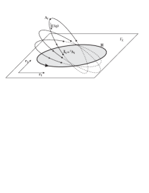
Figure 8: Gauge fixing surface $\Gamma_{\chi}$ for a fictitious problem. The shaded area is the reduced gauge fixing surface $\tilde{\Gamma}_{\chi}$ corresponding to one Gribov region and bounded by a Gribov horizon $H$ consisting of one gauge orbit.

One way to study the map (156), is to look for zeros of the corresponding Jacobian $\det J=|\partial A_{i}/\partial(r_{j},\varphi^{a})|$, which is proportional to the Faddeev-Popov determinant $\bigtriangleup_{\scriptscriptstyle\text{FP}}$ via equation (7). The zeros of $\det J$ form connected sets on the gauge fixing surface $\Gamma_{\chi}$, the Gribov horizons, which separate different Gribov regions from each other. Configurations in one Gribov region are related to configurations in another via discrete gauge transformations such as the shifts in (Coulomb gauge) Yang-Mills theory on a cylinder (cf. Section 4). One can eliminate this discrete residual gauge symmetry by restricting the domains of the gauge invariant variables $r_{j}$, like depicted in Fig. 8, where the shaded area (without the boundary!) corresponds to one Gribov region, the “reduced gauge fixing surface” $\tilde{\Gamma}_{\chi}$.

For the models studied in this paper, we found that the Gribov horizon contained residual gauge copies. In the case of the “$2\!\times\!2$”- and “$2\!\times\!3$-models” and for Yang-Mills theory on a cylinder (considering small gauge transformations only), the residual symmetries relating the gauge copies were continuous, giving rise to complete gauge orbits on the Gribov horizon. These continuous residual gauge symmetries have to be eliminated through additional gauge conditions, which imply the identification of gauge-equivalent points (“boundary identifications”). In Fig. 8, the Gribov horizon consists of one gauge orbit only. Choosing one representative on this orbit via a gauge condition $\chi^{\prime}$ amounts to the identification of all the points of the Gribov horizon with this point. It is easy to see that the resulting physical configuration space $\mathcal{M}$ is a 2-sphere $S^{2}$, which is topologically nontrivial, i.e. one needs at least two coordinate systems (charts) to cover $S^{2}$. For instance, we can interpret the shaded region in Fig. 8 as the coordinate neighborhood of one chart covering the North Pole of $S^{2}$, whereas the South Pole corresponding to all points on the Gribov horizon has to be excluded. This is very similar to what happens in $SU(2)$ Yang-Mills theory on a cylinder for small gauge transformations (ignoring global gauge symmetries), where the resulting configuration space is homeomorphic to $S^{3}$. Taking into account large gauge transformations in addition, the symmetry relating different points on the Gribov horizon becomes discrete. Nevertheless, upon identification of gauge equivalent configurations, the horizon disappears and we obtain a smooth manifold without boundaries or singular points. According to Singer [16], this should be generally true, as long as the gauge group acts freely on the configuration space $\mathcal{A}$. However, due to the boundary identifications, $\mathcal{M}$ will become topologically nontrivial.

This picture changes drastically, when the gauge group does not act freely on the configuration space. For instance, the zero configuration $A_{i}=0$ is invariant under all constant gauge transformations, so that its stability group is the entire structure group. As we have demonstrated within our models, the zero configuration becomes a singular point of the physical configuration space $\mathcal{M}$ after having divided out all gauge transformations. In general, such non-generic configurations, i.e. configurations with larger stability group, form manifolds of lower dimension in $\mathcal{M}$, so that $\mathcal{M}$ is no longer a manifold, but becomes a stratified variety [16, 62]. In particular, the physical configuration space $\mathcal{M}$ may have a genuine boundary of co-dimension $1$, which is to be distinguished from the fictitious boundary due to coordinate singularities [19, 63]. Accordingly, we cannot eliminate the zeros of the Jacobian, related to non-generic configurations. On the other hand, the zeros stemming from coordinate singularities are gauge (coordinate) dependent and, in some cases (cf. Sects. 2 and 3), may even disappear. As we have shown, however, these singular points do not introduce any new features into the theory. For example, solving our models on the gauge fixing surface $\Gamma_{\chi}$ without singular points yields the same results as the discussion on the physical configuration space $\mathcal{M}$, if in the first case, residual symmetries are implemented appropriately as symmetry conditions on the wave functions.

It is not clear, to what extent these results can be generalized to field theoretical models. For instance, the picture of Gribov regions separated by Gribov horizons and related via discrete residual gauge transformations may have to be modified. There may be more Gribov copies [8] inside the Gribov horizon, being not only due to large gauge transformations, as was the case in pure $SU(2)$ Yang-Mills theory on a cylinder. Nevertheless, it is to be expected that in general the physical configuration space $\mathcal{M}$ of gauge field theories will be topologically nontrivial, due to boundary identifications. For practical calculations, this will be most easily taken into account by defining wave functionals on the gauge fixing surface and implementing the residual gauge freedom via symmetry conditions on them. In addition, the nontrivial topology of $\mathcal{M}$ may modify the spectrum of the theory. For instance, in the case of non-Abelian gauge theories in $2\!+\!1$ dimensions, Feynman argued, that there is a mass gap in the gluon spectrum due to a maximal distance on the physical configuration space $\mathcal{M}$ [10]. Another approach currently being pursued is to analyze the influence of the nontrivial structure of $\mathcal{M}$ on the gluon propagator using the lattice as a regulator [24]. On the lattice, Gribov copies have been detected numerically upon choosing a maximally abelian gauge fixing [28, 29] which aims at a dual superconductor scenario of confinement. It is, however, not clear, how to obtain the physical configuration space in this case so that manifest gauge invariance is still an open question in this approach [64]. The presented formalism might also shed some light on these issues.

Acknowledgement

The authors are indepted to E. Werner for continued interest and support. They also thank S. Shabanov for enlightening discussions.

References

- [1] K.G. Wilson, Phys. Rev. D 10 (1974) 2445.
- [2] M. Creutz, Quarks, Gluons and Lattices (Cambridge University Press, Cambridge, 1983).
- [3] I. Montvay and G. Münster, Quantum fields on a lattice (Cambridge University Press, Cambridge, 1994).
- [4] J.D. Bjorken, Elements of Quantum Chromodynamics, Lectures on Lepton Nucleon Scattering and Quantum Chromodynamics, edited by A. Jaffe and D. Ruelle, pp. 423–561, Birkhäuser, Basel, 1982.
- [5] M. Lüscher, Nucl. Phys. B 219 (1983) 233.
- [6] J. Koller and P. Baal, Nucl. Phys. B 302 (1988) 1.
- [7] N.H. Christ and T.D. Lee, Phys. Rev. D 22 (1980) 939.
- [8] P. Baal, Nucl. Phys. B 369 (1992) 259.
- [9] P. Baal and B. Heuvel, Nucl. Phys. B 417 (1994) 215, hep-lat/9310005.
- [10] R.P. Feynman, Nucl. Phys. B 188 (1981) 479.
- [11] D. Karabali and V.P. Nair, Phys. Lett. B 379 (1996) 141, hep-th/9602155.
- [12] C.N. Yang and R.L. Mills, Phys. Rev. 96 (1954) 191.
- [13] H. Cheng and E.C. Tsai, Chin. J. of Phys. 25 (1987) 95.
- [14] V.N. Gribov, Nucl. Phys. B 139 (1978) 1.
- [15] R. Jackiw, Rev. Mod. Phys. 52 (1980) 661.
- [16] I.M. Singer, Commun. Math. Phys. 60 (1978) 7.
- [17] L.V. Prokhorov and S.V. Shabanov, Sov. Phys. Usp. 34 (1991) 108.
- [18] T. Heinzl, Nucl. Phys. B Proc. Suppl. 54 A (1997) 194, hep-th/9609055.
- [19] H. Yabuki, Ann. Phys. 252 (1996) 413.
- [20] Y.A. Simonov, Sov. J. Nucl. Phys. 41 (1985) 835.
- [21] P.E. Haagensen and K. Johnson, Nucl. Phys. B 439 (1995) 597, hep-th/9408164.
- [22] P. Baal, International workshop on nonperturbative approaches to QCD, Trento, Italy, 10-29 July, 1995, edited by D. Diakonov, pp. 4–23, 1995, hep-th/9511119, INLO-PUB-19/95.
- [23] D. Zwanziger, Nucl. Phys. B 412 (1994) 657.
- [24] D. Zwanziger, Nucl. Phys. B 485 (1997) 185, hep-th/9603203.
- [25] V.A. Franke and M.A. Semenov-Tyan-Shanskii, J. Sov. Math. 34 (1986) 1999.
- [26] W.I. Weisberger, Gribov ambiguities and quantization in the axial gauge, Asymptotic Realms of Physics, edited by A.H. Guth, K. Huang and R.L. Jaffe, pp. 162–185, MIT press, Cambridge, Mass., 1983.
- [27] G. Hooft, Nucl. Phys. B 190 (1981) 455.
- [28] G.S. Bali et al., Phys. Rev. D 54 (1996) 2863, hep-lat/9603012.
- [29] A. Hart and M. Teper, Phys. Rev. D 55 (1997) 3756, hep-lat/9606007.
- [30] R. Friedberg et al., Ann. Phys. 246 (1996) 381.
- [31] T.D. Lee, Particle Physics and Introduction to Field Theory (Harwood Academic Publishers, Chur, London, New York, 1981).
- [32] P.A.M. Dirac, Canad. J. Math. 2 (1950) 129.
- [33] O. Babelon and C.M. Viallet, Phys. Lett. 85 B (1979) 246.
- [34] O. Babelon and C.M. Viallet, Comm. Math. Phys. 81 (1981) 515.
- [35] M. Nakahara, Geometry, topology and physics (Institute of Physics Publishing, Bristol and Philadelphia, 1992).
- [36] A.C. Aitken and H.W. Turnbull, An introduction to the theory of canonical matrices (Dover Publishing Co, New York, 1961).
- [37] C. Martin and D. Vautherin, Ground state properties and glueball spectrum in SU(2) Yang-Mills theory using gauge invariant variables, hep-th/9401261, 1994.
- [38] S.G. Matinyan, G.K. Savvidi and N.G. Ter-Arutyunyan-Savvidi, Sov. Phys. JETP 53 (1981) 421.
- [39] G.K. Savvidy, Phys. Lett. 159 B (1985) 325.
- [40] F. Palumbo, Phys. Lett. B 199 (1987) 440.
- [41] I. Halperin, Ann. Phys. 244 (1995) 445, hep-ph/9503240.
- [42] S.J. Chang, Phys. Rev. D 29 (1984) 259.
- [43] C.C. Martens, R.L. Waterland and W.P. Reinhardt, J. Chem. Phys. 90 (1979) 2328.
- [44] J. Goldstone and R. Jackiw, Phys. Lett. 74 B (1978) 81.
- [45] F. Palumbo, M.I. Polykarpov and A.I. Veselov, Phys. Lett. B 258 (1991) 189.
- [46] P. Dahlqvist, J. Phys. A 25 (1992) 6265.
- [47] B. Simon, Ann. Phys. 146 (1983) 209.
- [48] C. Emmrich and H. Römer, Comm. Math. Phys. 129 (1990) 69.
- [49] S. Levit, Topics in QCD, Lecture Notes, GK-Workshop at Waischenfeld, Germany, 1991.
- [50] I.S. Gradshteyn and I.M. Ryzhik, Table of integrals, series and products (Academic Press Inc., New York, 1981).
- [51] A.A. Migdal, Sov. Phys. JETP 42 (1975) 413.
- [52] S.G. Rajeev, Phys. Lett. B 212 (1988) 203.
- [53] E. Langmann and G.W. Semenoff, Phys. Lett. B 303 (1993) 303, hep-th/9212038.
- [54] S.V. Shabanov, Phys. Lett. B 318 (1993) 323, hep-th/9308002.
- [55] O. Jahn, T. Kraus and M. Seeger, Int. J. Mod. Phys. A 12 (1997) 4445, hep-th/9610056.
- [56] G. Hooft, Nucl. Phys. B 153 (1979) 141.
- [57] E. Langmann, M. Salmhofer and A. Kovner, Mod. Phys. Lett. A 9 (1994) 2913, hep-th/9308115.
- [58] F. Lenz, H.W.L. Naus and M. Thies, Ann. Phys. 233 (1994) 317.
- [59] L. Chandar and E. Ercolessi, Nucl. Phys. B 426 (1994) 94, hep-th/9309065.
- [60] M.S. Marinov and M.V. Terentyev, Fortschr. Phys. 27 (1979) 511.
- [61] N.S. Manton, Ann. Phys. 159 (1985) 220.
- [62] J. Fuchs, M.G. Schmidt and C. Schweigert, Nucl. Phys. B 426 (1994) 107, hep-th/9404059.
- [63] H. Yabuki, Nucl. Phys. B 318 (1989) 464.
- [64] S.V. Shabanov, The monopole dominance in QCD, hep-th/9611228, 1996.