Dualities in Supergravity and Solvable Lie Algebras
Mario Trigiante

Department of Physics, University of Wales Swansea, Singleton Park,
Swansea SA2 8PP, United Kingdom

Abstract

The purpose of the present thesis is to give a self–contained review of the solvable Lie algebra approach to supergravity problems related with S, T and U dualities. After recalling the general features of dualities in both Superstring theory and Supergravity , we introduce the solvable Lie algebra formalism as an alternative description of the scalar manifold in a broad class of supergravity theories. It is emphasized how this mathematical technique on one hand allows to achieve a geometrical intrinsic characterization of Ramond–Ramond, Neveu–Schwarz and Peccei–Quinn scalars, once the supergravity theory is interpreted as the low energy limit of a suitably compactified superstring theory, on the other hand provides a convenient framework in which to deal with several non–perturbative problems. Using solvable Lie algebras for instance we find a general mechanism for spontaneous $N=2$ to $N=1$ local supersymmetry breaking. Moreover solvable Lie algebras are used to define a general method for studying systematically BPS saturated Black Hole solutions in supergravity.  

Chapter 0 Introduction

Recently considerable results were obtained towards a deeper understanding of some non–perturbative aspects of both superstring and supergravity theories. The basic concept underlying these latest developments is duality [5].

Superstring theory was originally introduced as a promising proposal for a fundamental quantum theory in which gravity is unified to the other elementary interactions in a consistent and finite framework. It is formulated in 10 space–time dimensions, but, if compactified to a D–dimensional space–time, it’s low–energy states are described by an effective D–dimensional N–extended supergravity theory. For a suitable choice of the initial superstring theory and of its compactification to 4 dimensions, the low–energy supergravity seems to have the right phenomenological content of fields to be the candidate for a theory describing our physical world. Nevertheless, superstring theory soon revealed not to be fundamental, since it is not unique. Indeed there are 5 known superstring theories (Type IIA, Type IIB, Type I, Heterotic $E_{8}\otimes E_{8}^{\prime}$, Heterotic $SO(32)$), and a supergravity in D–dimensions ($D<10$) usually describes the low–energy content of more than one superstring theory compactified on different manifolds. The discovery of string–string dualities made it possible to reduce the number of inequivalent superstring theories.

By string–string duality one denotes a correspondence between regimes of two different superstring theories which preserves the spectrum and the interactions. Such a correspondence allows to consider the two related theories as different mathematical descriptions of a same one. By exploiting the duality symmetries it was indeed possible to relate all the five known superstring theories and therefore view them as perturbative relizations on different backgrounds of a larger non–perturbative quantum theory in $11$ or $12$ space–time dimensions [13], [15] (named M-theory and F-theory respectively). Even if the physical content of the latter is not known so far, they are expected to admit all the known dualities as exact symmetries.

In order to characterize the concept of duality in a more precise fashion, let us consider a colsed superstring theory compactified on a $d$–dimensional compact manifold ${\cal K}_{d}$. The geometry of ${\cal K}_{d}$ is completely defined by the vacuum expectation values of certain low energy excitations, denoted by $t^{n}$, which define its moduli. Moreover, among the scalar $0$–modes of the superstring theory, the dilaton $\phi$ plays the important role of defining, through its vacuum expectation value, the string coupling constant $g$ : $g=exp\left(\langle\phi\rangle\right)$. The main feature of the scalars $t^{n}$ and $\phi$ is that they derive from fields which in the original $10$–dimensional string theory couple directly to the geometry of the world–sheet and are called (Neveu–Schwarz)–(Neveu–Schwarz) (NS). The remaining scalar $0$–modes are associated with the internal components (i.e. components along the directions of ${\cal K}_{d}$) of states in the original $10$–dimensional theory whose vacuum expectation values do not enter the superstring action. These states correspond to an even boundary condition for both the left and right fermionic movers of the closed string and are called Ramond–Ramond (RR) states. The corresponding scalar $0$–modes of the compactified theory are thus called Ramond–Ramond scalars. All the low–energy scalar excitations of the string theory compactified on ${\cal K}_{d}$ define the scalar content of a suitable effective N–extended supergravity theory in $D=10-d$ space–time dimensions.

Duality transformations are mappings between different backgrounds on which the superstring theory is realized. They are therefore represented by thansformations on the scalar fields of the low–energy supegravity, leaving the spectrum and the couplings of the string theory invariant. For instance the T–duality acts on the $t^{n}$ and RR scalars, leaving the dilaton invariant. Its action amounts to a transformation of the inner space geometry and is a generalization of the mapping $R\rightarrow\alpha^{\prime}/R$ ($\alpha^{\prime}$ being the string tension) for a string theory compactified on a circle. Since it does not affect $\phi$, it is perturbative that is it can be verified to be an exact symmetry of the theory order by order in the string coupling constant $g$. On the other hand, the effect of the conjectured S–duality, roughly speaking, is to map $\phi$ into $-\phi$, which implies the transformation $g\rightarrow 1/g$. It is therefore a non–perturbative duality which relates the strong coupling regime of a theory to the weak coupling regime on an other. In general, verifying the existence of a non–perturbative duality would require the knowledge of the complete non–perturbative spectrum of a given superstring theory which is not accessible since string theories are defined perturbatively. Therefore S–duality could only be conjectured. A common characteristic of both T and S–duality is that they do not mix RR and NS scalars.

Finally a larger non–perturbative U–duality was recently conjectured [14] whose main feature is to transform all the scalars into each other as if they were treated on an equal footing. U–duality therefore includes also transformations which do not preserve the RR or NS connotation of the scalar fields. The conjecture for the two non–perturbative S [53] and U [14] dualities was based on evidences drawn from the comparison between the perturbative spectrum of a string theory and some of its known non–perturbative BPS states.

Since suitably compactified superstring theories mapped into each other by duality transformations have the same low–energy effective field theory, dualities between superstring theories should be strictly related to global symmetries of the underlying supergravity. The latter, generally called hidden symmetries or dualities (in the supergravity framework) are well known and have been widely studied since the early eighties [37],[38]. Lets consider this relationship in more detail, for it shows that a proper starting point for a discussion on duality in superstring theory is the analysis of the global symmetries of its underlying low–energy effective theory.

In supergravity the scalar fields ($\Phi^{I}$) are described by a D–dimensional $\sigma$–model (D being the number of space–time dimensions), that is they are local coordinates of a non–compact Riemannian manifold ${\cal M}$ and the scalar action is invariant under the isometries of ${\cal M}$ (i.e. diffeomorphisms leaving the metric on ${\cal M}$ invariant). The isometry–group ${\cal G}$ of ${\cal M}$ is promoted to be a global symmetry–group of the field equations and the Bianchi identities when its action on the scalar fields is associated with a suitable transformation of the vectors or in general p–forms (duality transformation) entering the same supermultiplets as the scalars (this double action of ${\cal G}$ is required if supersymmetry is large enough, i.e. $N\geq 2$ in $D=4$). The NS scalars $\phi$ and $t^{n}$ span two submanifolds ${\cal M}_{s}$ and ${\cal M}_{t}$ of ${\cal M}$ respectively. In particular ${\cal M}_{t}$ is the moduli–space of the internal compact space ${\cal K}_{d}$ and its isometry group ${\cal G}_{t}\subset{\cal G}$ is a candidate for the T–duality group at the superstring level, since it leaves $\phi$ invariant. Nevertheless, it turns out that, in order to preserve the superstring energy levels, the T–duality group must be a suitable restriction to the integers ${\cal G}_{t}(Z)$ of ${\cal G}_{t}$. This statement was verified order by order in the string coupling expansion. In light of this observation, the previously mentioned S and U–duality conjectures may now be restated as the hypothesis that suitable descrete versions of the isometry group ${\cal G}_{s}$ of ${\cal M}_{s}$ and of the whole ${\cal G}$ correspond to the S and U–dualities respectively, at the superstring level. The restriction to the integers is required already in the framework of the effective supergravity once quantization conditions are taken into account i.e. once it is demanded that the hidden symmetries preserve the lattice spanned by the integer valued electric and magnetic charges carried by the solutions of the theory.

In order to retrieve the main ideas expressed so far, let us consider for instance type IIA superstring theory compactified on a six–torus (${\cal K}_{d}=T_{6}$). Its low–energy states are described by an $N=8$ supergravity in $D=4$ dimensions. The scalar manifold [37] is:

$${\cal M}\,=\,\frac{E_{7(7)}}{SU(8)}$$

The moduli $t^{n}$ of $T_{6}$ are $G_{ij}$ and $B_{ij}$ ($i=1,...,6$), internal components of the space–time metric $G_{MN}$ and the antisymmetric tensor field $B_{MN}$ in $10$–dimensions. They naturally span the moduli–space of $T_{6}$:

$${\cal M}_{t}\,=\,\frac{O(6,6)}{O(6)\otimes O(6)}$$

while the dilaton $\phi$ and the axion $B_{\mu\nu}$ span the manifold:

$${\cal M}_{s}\,=\,\frac{SL(2,{\rm I\kern-1.79993ptR})}{O(2)}$$

The isometry groups of these three manifolds are respectively: ${\cal G}=E_{7(7)}$, ${\cal G}_{t}=O(6,6)$ and ${\cal G}_{s}=SL(2,{\rm I\kern-1.79993ptR})$. The string–string T–duality group has been verified to be a restriction to the integers of ${\cal G}_{t}$, that is $O(6,6;Z)$, while the conjectured S and U–duality groups are $SL(2,Z)$ and $E_{7(7)}(Z)$ respectively.

As previously mentioned, evidences for these conjectures were drawn from the analysis of the BPS solitonic spectrum of the effective supergravity theory, under the hypothesis that these states already include the known BPS excitations of the fundamental string. BPS solitons are those solitonic solutions of a supergravity theory which saturate the Bogomolnyi bound, i.e. whose masses equal one or more eigenvalues of the central charge. If we consider theories having a large enough supersymmetry (e.g. $N\geq 4$ in $D=4$), the central charge is not affected by quantum corrections and therefore the value of the BPS mass computed semiclassically is exact. Moreover a duality transformed solution is still a solution of the supergravity theory since duality transformations are symmetries of the field equations and Bianchi identities. This property, together with the fact that the BPS condition is duality invariant, implies that all the BPS solitons of a supergravity theory fill a representation of the U–duality group (therefore also of the T and S–duality groups) suitably restricted to the integers ${\cal G}(Z)$ in order to preserve the charge lattice. The conjecture that ${\cal G}_{s}(Z)$ and the whole ${\cal G}(Z)$ are symmetries of the superstring spectrum requires the perturbative electrically charged string excitations fulfilling the BPS conditions to be in the same duality representation of a magnetically charged BPS soliton state of the low–energy effective supergravity (indeed S–duality exchanges electric and magnetic charges). But this state already belongs to a representation of ${\cal G}(Z)$ which is completely filled by BPS solitons, therefore the S and U–duality conjecture implies that the electrically charged superstring excitations fulfilling the BPS condition should be identified with equally charged BPS solitons of the low–energy effective theory. The fact that two superstring theories which differ at a perturbative level have, when compactified to a lower dimension, the same low–energy effective supergravity theory, and therefore the same BPS solitonic spectrum, is an evidence that they should correspond through a non perturbative duality. An example of two theories which are conjectured to be one the S-dual of the other is given by Type IIA superstring compactified on $K_{3}\times T_{2}$ and heterotic compactified on $T_{6}$. Their common low–energy effective theory is $D=4$, $N=4$ supergravity. In this case the S and U–duality groups of the two theories are : ${\cal G}_{s}(Z)=SL(2,Z)$ and ${\cal G}(Z)=SL(2,Z)\times O(6,22;Z)$.

0.1 Contents of the dissertation.

After this sketchy introduction to the concept of duality in superstring and supergravity theories, in what follows I will give an outline of the main topics discussed in the present thesis, posponing to the next chapters a more precise and complete analysis of some of the ideas introduced so far. All the problems which will be dealt with throughout the thesis are deeply related to the concept of duality in supergravity theories and their common denominator is a well extablished mathematical technique which has been applied for the first time in supergravity by our group: the solvable Lie algebras.

In the first chapter, after an introduction to electric-magnetic duality in supergravity and to Gaillard–Zumino model, the formalism of solvable Lie algebras will be introduced. The use of this technique, as it will be emphasized in the sequel, on one hand allows a considerable semplification of the mathematical structure of the scalar sector, on the other hand makes it possible to unravel the action of the U–duality on the scalar fields, revealing therefore to be a suitable mathematical laboratory for studying the non perturbative aspects of supergravity and hence of superstring theories. It will be shown that in many cases of interest, the scalar manifold ${\cal M}$ , which is a non–compact Riemannian manifold, may be described as a slovable Lie group manifold, locally generated therefore by a solvable Lie algebra. Since the supergravity action depends on the scalar manifold only through its local differential geometry, describing ${\cal M}$ as a group manifold allows to reformulate the scalar dependence of the action in an algebraic way which is much simpler since, for instance, differential operators on ${\cal M}$ correspond to linear mappings on the generating solvable algebra. Moreover such a new formulation allows to extablish a local correspondence between scalar fields and generators of the solvable algebra, this in turn yields a geometrical characterization of the RR and NS scalars and makes it possible to exploit the action of the S,T and U–duality groups on each of them. This analysis will be developed in the second chapter, where explicit examples of how the solvable Lie algebra machinery works will be given.

Another relevant potentiality of solvable Lie algebras is that they allow to determine easily the so called Peccei–Quinn scalars of a given theory, that is those scalars which appear in the supergravity action ’covered’ by a derivative and therefore are associated with global translational symmetries of the theory . The Peccei–Qiunn scalars turn out to be the parameters of the maximal abelian ideal ${\cal A}$ of the solvable algebra, which indeed generates all the possible translations on ${\cal M}$. Once the correspondence between scalar fields and generators of the solvable algebra has been extablished, it is strightforward to determine the RR and NS generators of ${\cal A}$. The latter act on RR Peccei-Quinn scalars translating them by a constant configuration. In order to introduce the topic of the third chapter, let us spend few words about RR fields and their charge. As previously mentioned, a characteristic of the RR fields is that they do not couple directly to the string. In $10$ dimensions the RR fields are higher order forms which can be thought of as the gauge fields corresponding to a certain $U(1)$–charges: the RR charges. Indeed it was recently conjectured that these fields couple solitonic extended objects [25] named D–branes, therefore the RR charges are solitonic (from the string point of view). In the effective low–energy supergravity, the RR scalars may be interpreted as D0–branes originated by wrapping the D–branes in higher dimension around the internal directions, and therefore they carry a solitonic RR charge.

The effect of a RR translation in ${\cal A}$ on a generic bosonic background is to generate a RR field. If this global symmetry is suitably gauged, i.e. made local by associating a vector field with it in a proper way, one may expect that the new theory admit vacua on which the RR scalar field has a non vanishing expectation value, i.e. vacua exhibiting a condensation of the RR charge [24]. Since D–branes were shown by Polchinski to saturate the Bogomolnyi bound, they share with BPS saturated states the property of preserving a certain fraction of the initial supersymmetries of the theory. Therefore the process of soliton condensation may yield to a spontaneous partial supersymmetry breaking. This mechanism was verified in the case of spontaneous $N=2\rightarrow N=1$ supersymmetry breaking in which the effective theory had a surviving quite general compact gauge group [16] but its general check for a generic N–extended supergravity is still work in prograss. In chapter 3, besides showing how gauging a RR translational isometry yields spontaneous supersymmetry breaking in the particular case of the $N=2$ theory mentioned above, emphasis will be given to the important role played by the solvable Lie algebras in solving the problem, since they allowed to determine easily not only ${\cal A}$ but also the flat directions of the scalar potential.

Finally the problem of finding the BPS solitonic solutions of a supergravity theory filling a U–duality representation is faced in Chapter 4 in the case of an $N=8$ theory [109]. In supergravity BPS solitons are Black Holes saturating the Bogomolnyi bound and, as previously pointed out, they have the property of preserving $1/2$, $1/4$ or $1/8$ of the original supersymmetries. We will be dealing with the latter kind of solitons. They are solutions of the second order field equations together with a system of first order equations deriving from the condition for the solution to have a residual number of supersymmetries (Killing spinor equations). The descriprion of the scalar manifold in terms of a solvable Lie algebra allows to formulate the problem in a geometrical fashion in which the first order equations are much easier to be solved. Moreover, using this formalism, it is possible to find the minimal number of scalars characterizing the generating solution of the U–duality orbit. Explicit calculations are carried out applying this approach to a simplified case in which the BPS Black Hole is characterized by the only dilaton fields.

Chapter 1 Duality in Supergravity and Solvable Lie Algebras

The first and most widely known example of duality in field theory is given by the symmetry of the Maxwell–Einstein equations in the vacuum

$$\partial_{\mu}F^{\mu\nu}\, = \,0$$

$$\partial_{\mu}\widetilde{F}^{\mu\nu}\, = \,0$$ (1.1)

with respect to a generic linear transformation mixing the electric field strenght $F^{\mu\nu}$ with its dual $\widetilde{F}^{\mu\nu}=(1/2)\epsilon^{\mu\nu\rho\sigma}F_{\rho\sigma}$ (duality rotation). It is apparent from eqs.1.1 that in presence of an electric current on the rhs of the first equation, a magnetic current should be introduced on the rhs of the second in order for the whole system to remain duality invariant. The requirement of duality symmetry in electromagnetism therefore implies the existence of magnetic charges.

A solution of the Maxwell–Einstein equations carrying magnetic charge $m$ (monopole) was initially found by P.A.M. Dirac [1]. He moreover obtained the following quantization condition which should be fulfilled by the electric charge $e$ and the magnetic charge $m$ in order for his solution to be physically consistent:

$$\frac{em}{4\pi\hbar}\,=\,\frac{n}{2}\quad\,\,n\in Z$$ (1.2)

Later ’t Hooft and Polyakov [2] found a monopole solution in a gauge theory with spontaneous symmetry breaking $SU(2)\rightarrow U(1)$ for which condition 1.2 was automatically fulfilled. The main ingredient used to find such a solution was the presence in the theory of scalar fields in the adjoint representation of the gauge group G. Their result is immediately generalized to a theory with generic compact non–abelian gauge group G describing scalar fields $\phi^{\alpha}\in{\it adj}(G)$. On a vacuum in which $\langle\phi^{\alpha}\rangle\neq 0$, $G$ is spontaneously broken to its Cartan subgroup ${\cal C}=U(1)^{r}\,;\,r=rankG$ (indeed, being ${\cal C}$ the little group of the adjoint representation it is the symmetry group of the vacuum). The ’t Hooft–Polyakov monopole is an example of soliton in field theory.

Since this kind of solution will play an important role in future analyses, I am going to spend few words about it. By soliton one denotes a stationary solution of the field equations with finite energy which corresponds to a boundary condition defining a topologically non trivial mapping between the sphere at infinity $S^{2}_{\infty}$ and the manifold of the degenerate scalar vacua $G/{\cal C}$. Such configurations are characterized by a conserved topological charge related to the element of $\pi_{2}(G/{\cal C})$ defined by their asymptotic behaviour. In the case of a monopole the topological charge coincides with its magnetic charge $m$. Denoting by $\phi_{o}=|\langle\phi^{\alpha}_{o}\rangle|$ the gauge invariant norm of the scalar vector corresponding to a chosen vacuum $V_{o}$, the effective theory on $V_{o}$ will have a spectrum of monopoles whose asymptotic behaviour fulfills the condition:

$$|\langle\phi^{\alpha}\rangle|_{S^{2}_{\infty}}=\phi_{o}$$ (1.3)

Bogomolnyi found that the mass of a monopole is bounded from below according to the condition:

$$M_{monopole}\,\geq\,4\pi\phi_{o}m\approx\frac{n}{e}\quad\,n\in Z$$ (1.4)

therefore in the perturbative regime of the theory ($e\approx 0$) monopoles are expected to be very massive.

One may think of monopoles as elementary excitations of a dual theory with gauge group given by the magnetic $U(1)^{r}$. The correspendence between a spontaneously broken non–abelian gauge theory and its abelian dual was first conjectured by Montonen and Olive [3]. The mapping between the elementary spactra of these two theories is non–perturbative since it is realized by the following duality transformations :

$$e \leftrightarrow m\approx\frac{n}{e}$$

$$B^{i}_{\mu} \leftrightarrow A^{i}_{\mu}$$ (1.5)

where $B^{i}_{\mu}$ are the the magnetic gauge fields defined in the following way:

$$\widetilde{F}^{i}=dB^{i}$$ (1.6)

The first of eqs.1.5 tells us that this duality maps the weak coupling regime of a theory into the strong coupling regime of its dual, while the second equation defines a transformation which is non–local and therefore can be a symmetry of, at most, the field equations and Bianchi identities, but not of the entire action. Moreover the transformations 1.5 should belong to a descrete group $\Gamma_{D}$ in order to preserve the lattices described by the magnetic and electric charges fulfilling the Dirac quantization condition 1.2.

In the case of electromagnetism, it is strightforward to check that the electric–magnetic duality transformations $\Gamma_{D}$ are a symmetry of the Maxwell equations in presence of electric and magnetic currents.

1.1 Duality in Supergravity:
the Gaillard–Zumino model.

Let us now turn on duality in a supersymmetric gauge theory. The following introduction to this topic will mainly refer to the presentation given in the review [73].

In order for a theory to exhibit electric-magnetic duality, it must have a non–perturbative spectrum of magnetic monopole solutions besides the electric fundamental excitations. As previously pointed out, the basic ingredient for the existence of ’t Hooft–Polyakov monopole solutions in a gauge theory is the presence of scalar fields transforming in the adjoint representation of the gauge group G. This requirement is automatically fulfilled in a four dimensional $N\geq 2$ supersymmetric gauge theory in which the gauge vectors $A^{\Lambda}_{\mu}\,;\,\Lambda=1,...,dim(G)$ are related through supersymmetry transformations to scalar fields $\phi^{\Lambda}$ in the same representation of G (i.e. the adjoint one). Moreover the fact that vector fields and scalars sit in the same supermultiplet requires the duality group $\Gamma_{D}$ to be a suitable discrete form of the isometry group of the scalar manifold, and gives these theories a particularly interesting mathematical structure, as I am going to show next.

Let us consider an N–extended supersymmetric model in $D=2p$ dimensions describing among the other fields a set of $n$ $(p-1)$–forms $A^{\Lambda}$ and $m$ sclalar fields $\phi^{I}$ belonging to the same supermultiplet. I shall restrict my treatment to the part of the action describing only the $A^{\Lambda}$ and $\phi^{I}$, which generalizes the Gaillard–Zumino action [38] to space–time dimensions greater than four. Moreover in this theory the $(p-1)$–forms do not gauge any non–abelian gauge group, therefore we can think of it as an abelian gauge theory with gauge group $U(1)^{n}$. As a starting hypothesis we will assume that all the fields are neutral with respect to this gauge group and therefore no electric or magnetic current will couple to the $(p-1)$–forms.

The scalar sector of a supergravity theory is described by a D–dimensional $\sigma$–model, which means that the scalar fields $\phi^{I}$ are local coordinates of a non–compact Riemannian manifold ${\cal M}$ and the scalar action $S_{scal}$ is required to be invariant with respect to the isometries ($t\in{\cal I}som({\cal M}$)) of ${\cal M}$, i.e. diffeomorphisms ($t\in{\it Diff}({\cal M}$)) on ${\cal M}$ leaving the metric $g$ invariant ($t^{*}g=g$). The action describing the scalars and the $(p-1)$–forms has the following structure:

$$S\, = \,S_{scal}\,+\,S_{(p-1)}\,=\,-\frac{1}{2}\int d^{D}\sqrt{-det(g)}g_{IJ}\partial_{\mu}\phi^{I}\partial^{\mu}\phi^{J}\,+$$

$$\frac{1}{2}\int d^{D}\left[(-)^{p}\gamma_{\Lambda\Sigma}(\phi)F^{\Lambda}\wedge\widetilde{F}^{\Sigma}\,+\,\theta_{\Lambda\Sigma}(\phi)F^{\Lambda}\wedge F^{\Sigma}\right]$$

where:

$$F^{\Sigma}\, = \,dA^{\Sigma}$$

$$\widetilde{F}^{\Sigma}\, = \,\frac{1}{p!}\epsilon_{\mu_{1}...\mu_{p}\sigma_{1}...\sigma_{p}}F^{\Sigma|\sigma_{1}...\sigma_{p}}dx^{\mu_{1}}\wedge....\wedge dx^{\mu_{p}}$$

$$\gamma_{\Lambda\Sigma}\, = \,\gamma_{\Sigma\Lambda}$$

$$\theta_{\Lambda\Sigma}\, = \,\theta_{\Sigma\Lambda}\,\,(p\,even)$$

$$\theta_{\Lambda\Sigma}\, = \,-\theta_{\Sigma\Lambda}\,\,(p\,odd)$$ (1.7)

The fact that the field–strenghts of the $(p-1)$–forms couple to the scalars through a generalized coefficient of the kinetic term $\gamma_{\Lambda\Sigma}(\phi)$ and a generalized theta–angle $\theta_{\Lambda\Sigma}(\phi)$ is a requirement of supersymmetry. Let us specialize the expression of the lagrangian describing the $(p-1)$–forms for $p$ even and $p$ odd and define in each case the magnetic field–strenght $G^{\Lambda}$ corresponding to the electric $F^{\Lambda}$:

p even

$${\cal L}\, = \,\frac{1}{2}\left[-\gamma_{\Lambda\Sigma}(\phi)F^{\Lambda}F^{\Sigma}\,-\,{\rm i}\theta_{\Lambda\Sigma}(\phi)F^{\Lambda}F^{*\Sigma}\right]$$

$$G^{*}_{\Lambda}\, = \,{\rm i}\frac{\delta{\cal L}}{\delta F^{\Lambda}}\,=\,{\rm i}\left(-\gamma_{\Lambda\Sigma}(\phi)F^{\Sigma}\,-\,{\rm i}\theta_{\Lambda\Sigma}(\phi)F^{*\Sigma}\right)$$

(1.8)

p odd

$${\cal L}\, = \,\frac{1}{2}\left[-\gamma_{\Lambda\Sigma}(\phi)F^{\Lambda}F^{\Sigma}\,+\,\theta_{\Lambda\Sigma}(\phi)F^{\Lambda}F^{*\Sigma}\right]$$

$$G^{*}_{\Lambda}\, = \,\frac{\delta{\cal L}}{\delta F^{\Lambda}}\,=\,\left(-\gamma_{\Lambda\Sigma}(\phi)F^{\Sigma}\,+\,\theta_{\Lambda\Sigma}(\phi)F^{*\Sigma}\right)$$

In both cases the field equations and the Bianchi identities have the following form:

$$\partial^{\mu}G^{*}_{\Lambda|\mu\mu_{1}...\mu_{p-1}}\, = \,0$$

$$\partial^{\mu}F^{*\Lambda}_{\mu\mu_{1}...\mu_{p-1}}\, = \,0$$ (1.10)

where we have introduced an involutive duality operation (*) on the field strenght $p$–forms defined as follows: $F^{*\Lambda}={\rm i}\widetilde{F}^{\Lambda}\,\,(p\,even)$ and $F^{*\Lambda}=\widetilde{F}^{\Lambda}\,\,(p\,odd)$. Eqs.1.10 are a generalization of eqs.1.1. By definition $S_{scal}$ is invariant with respect to the isometries of ${\cal M}$, but since the $(p-1)$–forms are related to the scalars by supersymmetry ($\Leftrightarrow$ they are coupled in $S_{p-1}$), a transformation on $\phi^{I}$ should have a couterpart also on the $(p-1)$–forms in order for at least the field equation and the Bianchi identities to remain invariant. Therefore, in order for ${\cal I}som({\cal M})$ to be promoted to a global symmetry group of the field equation and the Bianchi identities, it should have a suitable action also on the field strenghts $F^{\Lambda}$ and $G_{\Sigma}$ (duality transformation). The aim of the following calculations is to define such transformations.

It is useful to rewrite the quantities introduced so far in terms of the selfdual and anti–selfdual components $F^{(\pm)\Lambda}$ and $G_{\Sigma}^{(\pm)}$ of the electric and magnetic field strenghts:

$$F^{(\pm)\Lambda}\, = \,\frac{1}{2}\left(F^{\Lambda}\pm F^{*\Lambda}\right)$$

p even:

$${\cal L}\, = \,\frac{{\rm i}}{2}\left[{\cal N}_{\Lambda\Sigma}F^{+\Lambda}F^{+\Sigma}\,-\,{\overline{\cal N}}_{\Lambda\Sigma}F^{-\Lambda}F^{-\Sigma}\right]$$

$${\cal N}_{\Lambda\Sigma}\, = \,\theta_{\Lambda\Sigma}-{\rm i}\gamma_{\Lambda\Sigma}$$

$$G_{\Lambda}^{+}\, = \,{\cal N}_{\Lambda\Sigma}F^{+\Sigma}\,\,\,\,G_{\Lambda}^{-}\,=\,{\overline{\cal N}}_{\Lambda\Sigma}F^{-\Sigma}$$

p odd:

$${\cal L}\, = \,\frac{1}{2}\left[{\cal N}_{\Lambda\Sigma}F^{+\Lambda}F^{+\Sigma}\,+\,{\cal N}^{T}_{\Lambda\Sigma}F^{-\Lambda}F^{-\Sigma}\right]$$

$${\cal N}_{\Lambda\Sigma}\, = \,\theta_{\Lambda\Sigma}-\gamma_{\Lambda\Sigma}$$

$$G_{\Lambda}^{+}\, = \,{\cal N}_{\Lambda\Sigma}F^{+\Sigma}\,\,\,\,G_{\Lambda}^{-}\,=\,-{\cal N}^{T}_{\Lambda\Sigma}F^{-\Sigma}$$ (1.11)

where we have introduced a complex $n\times n$ field–dependent matrix ${\cal N}_{\Lambda\Sigma}(\phi)$. Our problem is to define, for a generic isometry $t$ on $\phi^{I}$, the corresponding transformation rule for ${\cal N}_{\Lambda\Sigma}$ and the linear transformation mixing $F^{(\pm)\Lambda}$ with $G_{\Sigma}^{(\pm)}$ of the form:

$$\left(\matrix{F^{(\pm)\Lambda}\cr G_{\Sigma}^{(\pm)}}\right)\,\rightarrow\,\left(\matrix{F^{(\pm)\prime\Lambda}\cr G^{(\pm)\prime}_{\Sigma}}\right)\,=\,\left(\matrix{A_{t}&B_{t}\cr C_{t}&D_{t}}\right)\left(\matrix{F^{(\pm)\Lambda}\cr G_{\Sigma}^{(\pm)}}\right)$$ (1.12)

$${\cal N}_{\Lambda\Sigma}(\phi)\,\rightarrow\,{\cal N}^{\prime}_{\Lambda\Sigma}(t(\phi))$$ (1.13)

which are demanded to be consistent with the definition of $G^{\Lambda}$ and, moreover, to leave eqs.1.10 invariant. The latter requirement is automatically fulfilled by the linear transformation defined in eq.1.12, while the former implies that the period matrix should transform by means of the following fractional linear transformation:

$${\cal N}^{\prime}(t(\phi))\, = \,\left(C_{t}+D_{t}{\cal N}(\phi)\right)\left(A_{t}+B_{t}{\cal N}(\phi)\right)^{-1}$$

p even:

$${\overline{\cal N}}^{\prime}(t(\phi))\, = \,\left(C_{t}+D_{t}{\overline{\cal N}}(\phi)\right)\left(A_{t}+B_{t}{\overline{\cal N}}(\phi)\right)^{-1}$$

p even:

$$-{\cal N}^{T\prime}(t(\phi))\, = \,\left(C_{t}-D_{t}{\cal N}^{T}(\phi)\right)\left(A_{t}-B_{t}{\cal N}^{T}(\phi)\right)^{-1}$$ (1.14)

Concistency of the second and the first of eqs.1.14 in the case $p$ even or of the third and the first in the case $p$ odd implies, for the linear transformation 1.12 the following condition:

$$\left(\matrix{A_{t}&B_{t}\cr C_{t}&D_{t}}\right)\in\matrix{Sp(2n,{\rm I\kern-1.79993ptR})&\mbox{p even}\cr SO(n,n)&\mbox{p odd}}$$ (1.15)

Summarizing the results described so far, the isometry group of the scalar manifold is promoted to be a global symmetry group of the field equations and the Bianchi identities once a double action on both scalar fields and field strenghts $p$–forms is defined by means of a suitable embedding $i_{\delta}$, which, in the two relevant cases, is:

$$i_{\delta}\,:\,\cases{{\cal I}som({\cal M})\longrightarrow Sp(2n,{\rm I\kern-1.79993ptR})&\mbox{p even}\cr{\cal I}som({\cal M})\longrightarrow SO(n,n)&\mbox{p odd}}$$ (1.16)

Under the action 1.12 of the duality group ${\cal G}=i_{\delta}({\cal I}som({\cal M}))$, the field strenghts $F^{\Lambda}$ and $G_{\Sigma}$ therefore transform as components of a symplectic or pseudo–orthogonal vector.

The model which we have considered so far may be thought of as describing the massless bosonic field content of a theory whose gauge group G, of rank m, was spontaneously broken to its Cartan subgroup $U(1)^{m}$ by a non vanishing expectation value of its scalar fields transforming in the $adj$ representation of G through a Higgs mechanism. Such mechanism would leave massless only those fields $A^{\Lambda}$ and $\phi^{I}$ which are neutral with respect to the residual $U(1)^{m}$ (the index $I$ labeling the Cartan directions of the adjoint representation on G), and generate a spectrum of massive electrically and magnetically charged states (the latter corresponding to ’t Hooft–Polyakov monopoles) coupled to the vector bosons $A^{\Lambda}$. Adopting this interpretation of the model, eqs.1.10 should be modified by the presence of electric and magnetic currents. We now define the following electric and magnetic charges:

$${\cal Q}=\left(\matrix{p^{\Lambda}\cr q_{\Sigma}}\right)=\left(\matrix{\int_{S^{2}_{\infty}}F^{\Lambda}\cr\int_{S^{2}_{\infty}}G_{\Sigma}}\right)\in\cases{Sp(2n,{\rm I\kern-1.79993ptR})&\mbox{p even}\cr SO(n,n)&\mbox{p odd}}$$ (1.17)

Besides the fundamental electrically charged excitations and the magnetic monopoles there are also dyonic colutions carrying both electric and magnetic charges $(p,q)$. Moreover, quantization implies that the charge vector ${\cal Q}$ must fulfill a symplectic (or pseudo–orthogonal) invariant generalization of condition 1.2 called Dirac–Schwinger–Zwanziger (DSZ) condition:

$$\left({\cal Q},{\cal Q}^{\prime}\right)=p^{\Lambda}q^{\prime}_{\Lambda}-p^{\prime\Lambda}q_{\Lambda}\in Z$$ (1.18)

where $\left(\,,\,\right)$ is the symplectic (or pseudo–orthogonal) invariant scalar product. Let us assume as hypothesis that all types of charges exist in the spectrum and let us fix a charge vector ${\cal Q}$, then the charge vector ${\cal Q}^{\prime}$ fulfilling eq.1.18 will describe a lattice, i.e. DSZ–condition implies that $p$ and $q$ are quantized. Requiring the action of the duality group ${\cal G}$ on the vector ${\cal Q}$ to leave the charge lattice invariant, the group ${\cal G}$ is spontaneously broken to a suitable restriction to the integers:

$${\cal G}\longrightarrow{\cal G}(Z)={\cal G}\cap\cases{Sp(2n,Z)&\mbox{p even}\cr SO(n,n;Z)&\mbox{p odd}}$$ (1.19)

The infinite discrete group ${\cal G}(Z)$ is the conjectured U–duality group in superstring theory, while the S and T duality, as we will see, will be suitable restrictions to the integers of well defined continous subgroups ${\cal G}_{s}$, ${\cal G}_{t}$ of ${\cal G}$.

For the sake of simplicity, let us restrict ourselves to the case of $D=4$ space–time dimensions. Our initial abelian $U(1)^{n}$ gauge theory may be also regarded as the fundamental theory prior to gauging. Performing the gauging procedure means to associate a certain number $k$ of vector fields $A^{\alpha}_{\mu}\,;\,\alpha=1,...,k$ with the generators of a non–abelian gauge group $G$ (dim$G=k$), subgroup of ${\cal I}som({\cal M})$ and to modify the lagrangian of the theory, by introducing $G$–covariant derivatives, coupling constants (one for each simple factor of $G$) and a suitable scalar potential in order to make the action locally invariant with respect to $G$. Gauging therefore, roughly speaking, means to promote a certain subgroup of isometries of ${\cal M}$ from global symmetries of the action to local symmetries. After gauging electric and magnetic currents will be present in the theory and the U–duality group will break to its discrete subgroup ${\cal G}(Z)$. As I mentioned earlier, not all the duality transformations in ${\cal G}$ are a symmetry of the action. Some of them indeed (those with $B_{t}\neq 0$ ) act on the charge vector ${\cal Q}$ by transforming the electric charges $q^{\Lambda}$ into a linear combination of electric and magnetic charges. Such transformations are obviously non–perturbative and they amount to a non–local transformation of the vector fields. Therefore they are not a global symmetry of the action and hence cannot be gauged. For instance the S–duality group ${\cal G}_{s}\subset{\cal G}$ is non–perturbative while the T–duality group ${\cal G}_{t}\subset{\cal G}$ is perturbative on the NS charges for its symplectic action on the corresponding field strenghts 1.12 is characterized by $B_{t}=0$. T–duality indeed leaves the perturbative expansions in the electric (NS) co

uplings invariant and in general it can be shown that upon restriction to the integers (as in 1.19) ${\cal G}_{t}$ is a symmetry of the action. By electric transformations one denotes those perturbative duality transformations having a diagonal action on the electric and magnetic charges and they are global symmetries of the lagrangian, with no need of any restriction to the integers. Finding the electric subgroup of ${\cal G}$ is therefore crucial in order to perform a gauging procedure and in next chapter we are going to deal with this problem.

Before electric and magnetic charged were switched on, the operation of conjugating the embedding $i_{\delta}$ by a symplectic (or pseudo–orthogonal) transformation (i.e. choice of a symplectic (or pseudo–orthogonal) gauge) is immaterial for it would lead to physically equivalent theories. In presence of charged states however, different choices of this gauge would lead to inequivalent theories (the intersection in eq.1.19 is indeed dependent on the choice of embeddings related to each other by means of a symplectic (or pseudo–orthogonal) transformation). The physical relevance, after gauging, of which symplectic (or pseudo–orthogonal) gauge is chosen for a given theory will be apparent in capter 3 where it will be shown how, in a four dimensional theory, the choice of a particular

symplectic gauge will be crucial in order for a mechanism of spontaneous supersymmetry breaking to occur. Our analysis so far has shown that studying the global symmetries of supergravity at the classical level, i.e. the isometries of the scalar manifold, is the first step towards a deeper understanding of dualities in superstring theories. For this reason, in what follows, I shall focus my analysis on the continuous versions of the S, T and U–dualities, which will be denoted by the same symbols as their discrete counterparts, seen as isometries of ${\cal M}$ and introduce a new description of the scalar manifold by means of solvable Lie algebras which reveals to have several advantages, as it will be apparent in the sequel.

An important feature of supergravity theories with sufficently large supersymmetry (e.g. in $D=4$ $N\geq 3$) is that the scalar manifold is an homogeneous manifold of the form:

$${\cal M}={\cal G}/{\cal H}\,;\quad\quad m=dim{\cal M}=dim{\cal G}-dim{\cal H}$$ (1.20)

where ${\cal G}$ has already been defined and ${\cal H}$ is its maximal compact subgroup. Since ${\cal M}$ is a non–compact Riemannian manifold, ${\cal G}$ is a non–compact real form of a semisimple Lie group. Writing the scalar manifold in the form 1.20 amounts to associate with each point $P$ of ${\cal M}$, parametrized by the scalar fields $(\phi^{I})$, a coset–representative ${\rm I\kern-1.79993ptL}(\phi)\in{\cal G}$ generated by the non-compact generators of ${\cal G}$ on which the action of a generic isometry $g\in{\cal G}$ on $\phi^{I}$ is defined as follows:

$$g:\phi\longrightarrow\phi^{\prime}\Leftrightarrow g\cdot{\rm I\kern-1.79993ptL}(\phi)\,=\,{\rm I\kern-1.79993ptL}(\phi^{\prime})\cdot h(g,\phi)$$ (1.21)

where $h(g,\phi)\in{\cal H}$ is called the compensator of the transformation $g$ on ${\rm I\kern-1.79993ptL}(\phi)$ (Figure 1.1).

Since, by definition, ${\cal G}$ is the isometry group of ${\cal M}$ embedded in $Sp(2n,{\rm I\kern-1.79993ptR})$ ($SO(n,n)$), eq.1.20 means that we are choosing a description of the scalar manifold in which the coset–representative is a symplectic (pseudo–orthogonal) $2n\times 2n$ matrix: ${\rm I\kern-1.79993ptL}(\phi)\equiv{\rm I\kern-1.79993ptL}(\phi)^{A}_{B}\in Sp(2n,{\rm I\kern-1.79993ptR})$ ($\in SO(n,n)$). So far we have considered the linear action of U–duality only on $(p-1)$–form potentials in an even D–dimensional space–time for which $D=2p$. As far as $n$ generic $(p^{\prime}-1)$–form potentials ($D\neq 2p^{\prime}$) are concerned, U–duality will act only on the corresponding $p^{\prime}$–forms field strenghts $F^{\Lambda}$ by means of a linear transformation belonging to the $n$–dimensional irreducible representation of ${\cal I}som({\cal M})$ which the $F^{\Lambda}$ belong to.

In next section I will show that a generic non–compact Riemannian manifold is isomorphic to a Lie group manifold ${\cal G}^{(s)}$ and therefore can be described locally in terms of a new coset–representative which is now a group element and whose parameters are the new local coordinates. The latter can be thought of as geodesic coordinates in the neighborhood of each point on ${\cal M}$. Indeed the transitive action of ${\cal G}^{(s)}$ on ${\cal M}$ needs no compensator, being the action of a group on its own manifold. In next chapter I will show how describing the scalar manifold in terms of a group manifold leads to a deeper understanding of different supergravity theories in diverse dimensions from a geometrical point of view and allow to exploit useful relations between them.

1.2 Homogeneous manifolds and
solvable Lie algebras.

Figure 1.1:

In this section we will deal with a general property according to which any homogeneous non-compact coset manifold may be expressed as a group manifold generated by a suitable solvable Lie algebra. [19]

Let us start by giving few preliminar definitions. A solvable Lie algebra $Solv$ is a Lie algebra whose $n^{th}$ order (for some $n\geq 1$) derivative algebra vanishes:

$${\cal D}^{(n)}Solv = 0$$

$${\cal D}Solv=[Solv,Solv] \quad{\cal D}^{(k+1)}Solv=[{\cal D}^{(k)}Solv,{\cal D}^{(k)}Solv]$$ ;

A metric Lie algebra $(\,\hbox{$\vrule height=6.45831pt,width=0.4pt,depth=0.0pt\kern-3.00003pt{\rm G}$},\langle,\rangle)$ is a Lie algebra endowed with an euclidean metric $\langle,\rangle$. An important theorem states that if a Riemannian manifold $({\cal M},g)$ admits a transitive group of isometries ${\cal G}_{s}$ generated by a solvable Lie algebra $Solv$ of the same dimension as ${\cal M}$, then:

$${\cal M}\sim{\cal G}_{s} = exp(Solv)$$

$$g_{|e\in{\cal M}} = \langle,\rangle$$

where $\langle,\rangle$ is an euclidean metric defined on $Solv$. Therefore there is a one to one correspondence between Riemannian manifolds fulfilling the hypothesis stated above and solvable metric Lie algebras $(Solv,\langle,\rangle)$.
Consider now an homogeneous coset manifold ${\cal M}={\cal G}/{\cal H}$, ${\cal G}$ being a non compact real form of a semisimple Lie group and ${\cal H}$ its maximal compact subgroup. If  $\vrule height=6.45831pt,width=0.4pt,depth=0.0pt\kern-3.00003pt{\rm G}$ is the Lie algebra generating ${\cal G}$, the so called Iwasawa decomposition ensures the existence of a solvable Lie subalgebra $Solv\subset\,\hbox{$\vrule height=6.45831pt,width=0.4pt,depth=0.0pt\kern-3.00003pt{\rm G}$}$, acting transitively on ${\cal M}$, such that [18]:

$$\,\hbox{$\vrule height=6.45831pt,width=0.4pt,depth=0.0pt\kern-3.00003pt{\rm G}$}={\rm I\kern-1.79993ptH}\oplus Solv\qquad\mbox{dim }Solv=\mbox{dim }{\cal M}$$

${\rm I\kern-1.79993ptH}$ being the maximal compact subalgebra of  $\vrule height=6.45831pt,width=0.4pt,depth=0.0pt\kern-3.00003pt{\rm G}$ generating ${\cal H}$.
In virtue of the previously stated theorem, ${\cal M}$ may be expressed as a solvable group manifold generated by $Solv$. The algebra $Solv$ is constructed as follows [18]. Consider the Cartan decomposition

$$\,\hbox{$\vrule height=6.45831pt,width=0.4pt,depth=0.0pt\kern-3.00003pt{\rm G}$}={\rm I\kern-1.79993ptH}\oplus{\rm I\kern-1.79993ptK}$$ (1.22)

where ${\rm I\kern-1.79993ptK}$ is the subspace consisting of all the non compact generators of  $\vrule height=6.45831pt,width=0.4pt,depth=0.0pt\kern-3.00003pt{\rm G}$. Let us denote by ${\cal C}_{K}$ the maximal abelian subspace of ${\rm I\kern-1.79993ptK}$ and by ${\cal C}$ the Cartan subalgebra of  $\vrule height=6.45831pt,width=0.4pt,depth=0.0pt\kern-3.00003pt{\rm G}$. It can be proven [18] that ${\cal C}_{K}={\cal C}\cap{\rm I\kern-1.79993ptK}$, that is it consists of all non compact elements of ${\cal C}$. Furthermore let $h_{\alpha_{i}}$ denote the elements of ${\cal C}_{K}$, $\{\alpha_{i}\}$ being a subset of the positive roots of  $\vrule height=6.45831pt,width=0.4pt,depth=0.0pt\kern-3.00003pt{\rm G}$ and $\Delta^{+}$ the set of positive roots $\beta$ not orthogonal to all the $\alpha_{i}$ (i.e. the corresponding “shift” operators $E_{\beta}$ do not commute with ${\cal C}_{K}$). It can be demonstrated that the solvable algebra $Solv$ defined by the Iwasawa decomposition may be expressed in the following way:

$$Solv={\cal C}_{K}\oplus\{\sum_{\alpha\in\Delta^{+}}E_{\alpha}\cap\,\hbox{$\vrule height=6.45831pt,width=0.4pt,depth=0.0pt\kern-3.00003pt{\rm G}$}\}$$ (1.23)

where the intersection with  $\vrule height=6.45831pt,width=0.4pt,depth=0.0pt\kern-3.00003pt{\rm G}$ means that $Solv$ is generated by those suitable complex combinations of the “shift” operators which belong to the real form of the isometry algebra  $\vrule height=6.45831pt,width=0.4pt,depth=0.0pt\kern-3.00003pt{\rm G}$.

The rank of an homogeneous coset manifold is defined as the maximum number of commuting semisimple elements of the non compact subspace ${\rm I\kern-1.79993ptK}$. Therefore it coincides with the dimension of ${\cal C}_{K}$, i.e. the number of non compact Cartan generators of  $\vrule height=6.45831pt,width=0.4pt,depth=0.0pt\kern-3.00003pt{\rm G}$. A coset manifold is maximally non compact if ${\cal C}={\cal C}_{K}\subset Solv$. As we will see this kind of manifolds corresponds to the scalar manifold of the so called maximally extended supergravities, that is D–dimensional supergravity theories, whose supersymmetry is the maximal allowed by the space–time dimension D.

It is useful to spend few words about the relation between the two descriptions of ${\cal M}$ considered so far, i.e. coset manifold and the group manifold ${\cal G}^{(s)}$. In the former case each point $P$ of ${\cal M}$ is associated with a coset–representative ${\rm I\kern-1.79993ptL}(P)\in Exp({\rm I\kern-1.79993ptK})$ which is not a group element, being ${\rm I\kern-1.79993ptK}$ not an algebra, in the latter case, on the other hand, the same point is described by a group element ${\rm I\kern-1.79993ptL}_{s}(P)\in{\cal G}^{(s)}\approx Exp(Solv)$. The two transformations ${\rm I\kern-1.79993ptL}(P)$ and ${\rm I\kern-1.79993ptL}_{s}(P)$ belong to the same equivalence class with respect to the right multiplication by an element of ${\cal H}$:

$${\rm I\kern-1.79993ptL}(P)\,=\,{\rm I\kern-1.79993ptL}_{s}(P)\cdot h(P)\,;\quad h(P)\in{\cal H}$$ (1.24)

Differently from ${\rm I\kern-1.79993ptL}$, whatever point $P$ on ${\cal M}$ may be reached from a fixed origin $O\in{\cal M}$ by the left action of a suitable group element of ${\cal G}^{(s)}$ on ${\rm I\kern-1.79993ptL}_{s}(O)$ , with no need of any compensator, being ${\cal G}^{(s)}$ a group of transitive isometries on ${\cal M}$:

$${\rm I\kern-1.79993ptL}_{s}(P)\,=\,g(P,O)\cdot{\rm I\kern-1.79993ptL}_{s}(O)\,;\quad g(P,O)\in{\cal G}^{(s)}$$ (1.25)

As far as the action of the whole isometry group ${\cal G}$ on ${\cal M}$ is concerned, the best description of the latter is the coset manifold one, since $Solv$ is not stable with respect to the adjoint action of the compact subalgebra ${\rm I\kern-1.79993ptH}$ while ${\rm I\kern-1.79993ptK}$ on the other hand is. Therefore, starting from the parametrization of a point $P\in{\cal M}$ by means of solvable coordinates $\phi^{I}(P)$ defined by:

$${\rm I\kern-1.79993ptL}_{s}(\phi(P))\,=\,\exp{\left(\phi^{I}T_{I}\right)}\,;\quad\phi^{I}T_{I}\in Solv$$ (1.26)

$T_{I}$ being the generators of $Solv$ in eq.1.23, the transformation rules of $\phi^{I}$ under the action of a generic isometry $g\in{\cal G}$ in are defined in the following way:

$$g:\,P\, \longrightarrow \,P^{\prime}$$

$${\rm I\kern-1.79993ptL}_{s}(\phi(P)) \rightarrow {\rm I\kern-1.79993ptL}(P)\,{\stackrel{{\scriptstyle g}}{{\longrightarrow}}}\,{\rm I\kern-1.79993ptL}(P^{\prime})\,\rightarrow\,{\rm I\kern-1.79993ptL}_{s}(\phi^{\prime}(P^{\prime}))$$ (1.27)

where the first and the last arrows refer to a transformation from the group description to the coset manifold description and vice versa, while the middle arrow refers to the isometry transformation in the coset manifold formalism as described in eq. 1.21.

One of the main reasons for choosing to describe a scalar manifold ${\cal M}$ in terms of a solvable Lie algebra is that in this formalism the scalar fields $\phi^{I}$ are interpreted as the local solvable coordinates defined in eq. 1.26 which means to extablish a local one to one correspondence between the scalars and the generators $T_{I}$:

$$\phi^{I}\longleftrightarrow T_{I}\,;\quad I=1,...,m=dim{\cal M}$$ (1.28)

As we will se in next chapter, such a correspondence comes out in a quite natural way and allows on one hand to define, through the procedure represented in eq. 1.27, the trasformation rule of each scalar field under the U–duality group ${\cal G}$, on the other hand to achieve a geometrical intrinsic characterization of the scalars and in particular of the RR and NS sectors. An other considerable advantage of using metric solvable Lie algebras $(Solv,\langle,\rangle)$ is that the local differential geometry of the scalar manifold is described in terms of algebraic structures. In particular differential operators on ${\cal M}$ such as the covariant derivative and the Riemann tensor correspond to linear operators on the generating solvable Lie algebra $Solv\sim T_{p}{\cal M}$ in the neighborhood of a generic point $p\in{\cal M}$:

$$\bigtriangledown_{X} \longrightarrow L_{X}\,\,(\mbox{Nomizu operator})\,\,\,\forall x\in Solv$$

$$R(X,Y) \longrightarrow Riem(X,Y)\,\,(\mbox{Riemann operator})\,\,\,\forall X,Y\in Solv$$ (1.29)

where the Nomizu operator $L_{X}\,:Solv\rightarrow Solv$ is defined in the following way:

$$\forall X,Y,Z\in Solv : 2<Z,L_{X}Y>$$ (1.30)

$$= <Z,[X,Y]>-<X,[Y,Z]>-<Y,[X,Z]>$$

and the Riemann curvature 2–form $Riem(X,Y)\,:Solv\rightarrow Solv$ is given by the commutator of two Nomizu operators:

$$<W,\{[L_{X},{\rm I\kern-1.79993ptL}_{Y}]-L_{[X,Y]}\}Z>=Riem^{W}_{\ Z}(X,Y)$$ (1.31)

Since the action of a supergravity theory depends on the scalar manifold only through its local differential properties, such a new formalism allows to describe the scalar dependence of the theory through an algebraic structure which is much simpler to master.

To end this section I will give an explicit example of Iwasawa decomposition Vs Cartan decomposition for the semisimple group ${\cal G}=SL(3,{\rm I\kern-1.79993ptR})$. The positive roots of ${\cal G}$ are:

$$\alpha_{1}=\epsilon_{1}-\epsilon_{2}\,;\,\,\alpha_{2}=\epsilon_{2}-\epsilon_{3}\,;\,\,\alpha_{3}=\epsilon_{1}-\epsilon_{3}$$ (1.32)

Let $\lambda_{i}\,;\,i=1,...,8$ denote a basis for the Lie algebra  $\vrule height=6.45831pt,width=0.4pt,depth=0.0pt\kern-3.00003pt{\rm G}$ of ${\cal G}$ consistent with the Cartan decomposition.

$$\mbox{{\bf Cartan decomposition: }}\,\hbox{$\vrule height=6.45831pt,width=0.4pt,depth=0.0pt\kern-3.00003pt{\rm G}$}\,=\,{\rm I\kern-1.79993ptH}\oplus{\rm I\kern-1.79993ptK}$$

$${\rm I\kern-1.79993ptH}\,=\,\left[\matrix{\lambda_{6}=\left(\matrix{0&1&0\cr-1&0&0\cr 0&0&0}\right)&\lambda_{7}=\left(\matrix{0&0&1\cr 0&0&0\cr-1&0&0}\right)\cr\lambda_{8}=\left(\matrix{0&0&0\cr 0&0&1\cr 0&-1&0}\right)&\phantom{\matrix{0&0&1\cr 0&0&0\cr 1&0&0}}}\right]$$

$${\rm I\kern-1.79993ptK}\,=\,\left[\matrix{\lambda_{1}=\left(\matrix{1&0&0\cr 0&0&0\cr 0&0&-1}\right)&\lambda_{2}=\left(\matrix{0&0&0\cr 0&1&0\cr 0&0&-1}\right)\cr\lambda_{3}=\left(\matrix{0&1&0\cr 1&0&0\cr 0&0&0}\right)&\lambda_{4}=\left(\matrix{0&0&1\cr 0&0&0\cr 1&0&0}\right)\cr\lambda_{5}=\left(\matrix{0&0&0\cr 0&0&1\cr 0&1&0}\right)&\phantom{\matrix{0&0&1\cr 0&0&0\cr 1&0&0}}}\right]$$

$$\mbox{{\bf Iwasawa decomposition: }}\,\hbox{$\vrule height=6.45831pt,width=0.4pt,depth=0.0pt\kern-3.00003pt{\rm G}$}\,=\,{\rm I\kern-1.79993ptH}\oplus Solv$$

$$Solv\,=\,\left[\matrix{\lambda_{1}=\left(\matrix{1&0&0\cr 0&0&0\cr 0&0&-1}\right)&\lambda_{2}=\left(\matrix{0&0&0\cr 0&1&0\cr 0&0&-1}\right)\cr E_{\alpha_{1}}=\left(\matrix{0&1&0\cr 0&0&0\cr 0&0&0}\right)&E_{\alpha_{2}}=\left(\matrix{0&0&0\cr 0&0&1\cr 0&0&0}\right)\cr E_{\alpha_{3}}=\left(\matrix{0&0&1\cr 0&0&0\cr 0&0&0}\right)&\phantom{\matrix{0&0&1\cr 0&0&0\cr 0&0&0}}}\right]$$ (1.33)

Siunce the Cartan subalgebra ${\cal C}$ is generated by $\{\lambda_{1},\lambda_{2}\}$ which are non–compact, it follows that ${\cal C}={\cal C}_{K}$ and the algebra is maximally non compact. The solvable algebra $Solv$ is the direct sum of ${\cal C}$ and the nilpotent generators corresponding to all the positive roots, according to eq.1.23.

1.3 Kählerian, Quaternionic algebras and c–map.

In this last section, I will specialize the solvable algebra machinery to the case of Kählerian and Quaternionic manifolds which are of great interest in some supergravity theories. The main reference which I will follow in this treatment is [19], even if I will give just the main results which will be useful for a later analysis, skipping the mathematical details.

Let us breifly recall the definitions of Special Kähler (of local type) and of Quaternionic manifolds whose geometries characterize the scalar sector of $N=2$ supergravity theories. For a complete analysis of their properties see [73].

1.3.1 Special Kähler manifolds.

Consider a complex n–dimensional manifold ${\cal M}$ endowed with a complex structure $J\in End(T{\cal M})$, $J^{2}=-Id$ and a metric $g$, hermitian with respect to $J$, i.e.

$$g(J\cdot w\,,\,J\cdot u)\,=\,g(w\,,\,u)\,;\quad\forall w,u\in T{\cal M}$$ (1.34)

Referring to a well adapted basis of $T{\cal M}$ $(\partial/\partial z^{i}\,;i=1,...,n\,\,:J\cdot\partial/\partial z^{i}={\rm i}\partial/\partial z^{i})$, hermiticity of $g$ implies that $g_{ij}=g_{i^{\star}j^{\star}}=0$ and its reality that $g_{i\star j}=g_{ij^{\star}}$. Let us now introduce the differential $2$–form $K$:

$$K(w\,,\,u)\,=\,\frac{1}{2\pi}g(J\cdot w\,,\,u)\,;\quad\forall w,u\in T{\cal M}$$ (1.35)

whose expression in a local coordinate patch is:

$$K\,=\,\frac{{\rm i}}{2\pi}g_{ij^{\star}}dz^{i}\wedge d\overline{z}^{j^{\star}}$$ (1.36)

The hermitian manifold ${\cal M}$ is called a Kähler manifold iff:

$$dK\,=\,0$$ (1.37)

Equation 1.37 is a differential equation for $g_{ij^{\star}}$ whose general solution in a generic local chart is given by the expression:

$$g_{ij^{\star}}\,=\,\partial_{i}\partial_{j^{\star}}{\cal K}$$ (1.38)

where the real function ${\cal K}={\cal K}^{\star}={\cal K}(z,\overline{z})$ is named Kähler potential. and is defined up to the real part of an holomorohic function. Let us now introduce a bundle ${\cal Z}\rightarrow{\cal M}$ of the form ${\cal Z}={\cal L}\otimes{\cal SV}$ where ${\cal L}\rightarrow{\cal M}$ is a line bundle whose first chern class equals the cohomology class of $K$ ($\Rightarrow{\cal M}$ is Hodge Kähler manifold), and ${\cal SV}\rightarrow{\cal M}$ is a symplectic bundle with structure group $Sp(2n+2,{\rm I\kern-1.79993ptR})$.

Definition: ${\cal M}$ is a Special Kähler manifold of local type iff there exist a holomorphic section $\Omega\in\Gamma({\cal Z},{\cal M})$

$$\Omega(z)\,=\,\left(\matrix{X^{\Lambda}(z)\cr F_{\Sigma}(z)}\right)$$ (1.39)

such that:

$$K\, = \,\frac{{\rm i}}{2\pi}\partial\overline{\partial}\left({\rm i}\langle\Omega,\overline{\Omega}\rangle\right)$$

$$\langle\partial_{i}\Omega,\partial_{j}\Omega\rangle\, = \,0$$

$${\rm i}\langle\Omega,\overline{\Omega}\rangle {\stackrel{{\scriptstyle def}}{{=}}} {\rm i}\left(\overline{X}^{\Lambda}F_{\Lambda}\,-\,\overline{F}_{\sigma}X^{\sigma}\right)$$ (1.40)

The $n$ complex scalar fields belonging to $n$ vector multiplets of a $N=2$ supergravity theory span a Special Kähler manifold.

1.3.2 Quaternionic manifolds.

The hyperscalars of an $N=2$ supergravity theory on the other hand turn out to parametrize a Quaternionic manifold ${\cal QM}$ which I am about to define.

Consider a $4m$ dimensional real manifold ${\cal QM}$ endowed with three complex structures $J^{\alpha}:T{\cal QM}\rightarrow T{\cal QM}\,;\,\alpha=1,2,3$ such that:

$$J^{\alpha}J^{\beta}\,=\,-\delta^{\alpha\beta}{\rm 1\kern-3.50006pt1}\,+\,\epsilon^{\alpha\beta\gamma}J^{\gamma}$$ (1.41)

and a metric $h$ which is hermitian with respect to them:

$$h(J^{\alpha}\cdot w\,,\,J^{\alpha}\cdot u)\,=\,h(w\,,\,u)\,;\quad\forall w,u\in T{\cal QM}\,;\,\alpha=1,2,3$$ (1.42)

Let us introduce a triplet of $SU(2)$ Lie–algebra valued $2$–forms $K^{\alpha}$ (Hyper Kähler forms):

$$K^{\alpha}\,=\,K^{\alpha}_{uv}dq^{u}\wedge dq^{v}\,=\,h_{uw}{J^{\alpha}}^{w}_{v}dq^{u}\wedge dq^{v}\,;\,u,v=1,...,4m$$ (1.43)

Moreover let a principal $SU(2)$–bundle ${\cal SU}\rightarrow{\cal QM}$ be defined, whose connection is denoted by $\omega^{\alpha}$ and such that:

$$\bigtriangledown K^{\alpha}\,{\stackrel{{\scriptstyle def}}{{=}}}\,dK^{\alpha}\,+\,\epsilon^{\alpha\beta\gamma}\omega^{\beta}\wedge K^{\gamma}\,=\,0$$ (1.44)

Definition: ${\cal QM}$ is a Quaternionic manifold iff the curvature of the ${\cal SU}$ bundle $\Omega^{\alpha}$

$$\Omega^{\alpha}\,{\stackrel{{\scriptstyle def}}{{=}}}\,d\omega^{\alpha}\,+\,\frac{1}{2}\epsilon^{\alpha\beta\gamma}\omega^{\beta}\wedge\omega^{\gamma}$$ (1.45)

is proportional to the Hyper Kähler 2–forms:

$$\Omega^{\alpha}\,=\,\frac{1}{\lambda}K^{\alpha}$$ (1.46)

$\lambda$ being a non vanishing real number. The holonomy group of ${\cal QM}$ turns out to be the direct product of $SU(2)$ and of $Sp(2m;{\rm I\kern-1.79993ptR})$.

1.3.3 Alekseevskii’s formalism.

There is a wide class of Quaternionic and Special Kähler manifolds (${\cal QM}$, ${\cal SK}$) (not necessarely homogeneous) which admit a solvable group of transitive isometries (with no fixed point). By definition, these manifold are called normal. In virtue of the main theorem stated in last section, they are in one to one correspondence with suitable solvable Lie algebras which are hence named quaternionic and Kählerian algebras respectively. In the sequel I will denote a quaternionic metric algebra by $(V,\langle,\rangle)$ and a Kählerian metric algebra by $(W,\langle,\rangle)$ :

$${\cal QM}\, \approx \,\exp{V}$$

$${\cal SK}\, \approx \,\exp{W}$$ (1.47)

In the seventies Alekseevskii faced the problem of classifying the normal quaternionic manifolds through their generating quaternionic algebras and found an interesting correspondence between the latter and certain Kählerian algebras, later called the c–map. All the quantities defined for ${\cal QM}$ and ${\cal SK}$ have their algebraic couterpart on $(V,\langle,\rangle)$ and $(W,\langle,\rangle)$, such as the quaternionic structure $J^{\alpha}:\,V\rightarrow V$ for the former and the complex structure $J:\,W\rightarrow W$ for the latter, fulfilling eq. 1.41 and $J^{2}=-Id$ respectively.

The quaternionic algebras $V$ which we will be interested in, have the following structure:

$$V\, = \,U\oplus\widetilde{U}$$

$$U\, = \,F_{0}\oplus W$$

$$\widetilde{U}\, = \,\widetilde{F}_{0}\oplus\widetilde{W}$$

$$J^{1}\cdot U\, = \,U\,\,\,J^{2}\cdot U\,=\,\widetilde{U}$$ (1.48)

where $F_{0}$ and $\widetilde{F}_{0}$ are defined in the following way:

$$F_{0}\, = \,\{e_{0}\,,\,e_{1}\}$$

$$\widetilde{F}_{0}\, = \,\{e_{2}\,,\,e_{3}\}$$

$$\widetilde{F}_{0}\, = \,J^{2}\cdot F_{0}$$

$$\left[e_{0}\,,\,e_{1}\right]\, = \,e_{1}\,\,;\,\,\left[e_{1}\,,\,e_{2}\right]\,=\,0$$

$$\left[e_{0}\,,\,e_{2}\right]\, = \,e_{2}\,\,;\,\,\left[e_{1}\,,\,e_{3}\right]\,=\,0$$

$$\left[e_{0}\,,\,e_{3}\right]\, = \,e_{3}\,\,;\,\,\left[e_{2}\,,\,e_{3}\right]\,=\,0$$ (1.49)

where $e_{i}\,\,i=0,1,2,3$ are orthonormal with respect to $\langle,\rangle$. Moreover the following relations hold:

$$\left[e_{1}\,,\,W\oplus\widetilde{U}\right]\, = \,0$$

$$\left[e_{0}\,,\,\widetilde{U}\right]\, = \,\frac{1}{2}\,\widetilde{U}$$

$$\left[e_{0}\,,\,W\right]\, = \,0$$

$$\left[U\,,\,U\right]\,\subset\,U\,\quad\left[U\,,\,\widetilde{U}\right]\, \subset \,\widetilde{U}\,\quad\left[\widetilde{U}\,,\,\widetilde{U}\right]\,\subset\,\{e_{1}\}$$ (1.50)

$(F_{0},J^{1}_{|F_{0}})$ and $(W,J^{1}_{|W})$ are Kählerian algebras whose complex structure is the restriction of $J^{1}$ on them. $F_{0}$, defined by 1.49 is called key algebra with weight one (it is strightforward to check that a key algebra is the solvable algebra generating the homogeneous manifold $SU(1,1)/U(1)$). The mapping $Adj_{U}\,:\,\widetilde{U}\rightarrow\widetilde{U}$ defines a representation of the Kählerian algebra $U$ on the subspace $\widetilde{U}$. With respect to a new complex structure introduced on $\widetilde{U}$ as follows:

$$\widetilde{J}_{\widetilde{F}_{0}}{\stackrel{{\scriptstyle def}}{{=}}}J^{1}\,;\,\,\quad\widetilde{J}_{\widetilde{W}}{\stackrel{{\scriptstyle def}}{{=}}}-J^{1}$$ (1.51)

one finds that $Adj$ fulfills the axioms defining a Q–representation. The most relevant of them tells that $Adj$ is a symplectic representation with respect to $\widetilde{J}$. Thus $U$ and in particular $W$ is a Kählerian algebra having a Q–representation and it was shown that there is a one to one correspondence (c–map) between quaternionic algebras of the kind 1.48 and Kählerian algebras $W$ admitting a Q–representation.

$$V(\mbox{quat. algebra}){\stackrel{{\scriptstyle\mbox{c--map}}}{{\leftrightarrow}}}W(\mbox{k\"{a}h. algebra + Q--repr.})$$ (1.52)

Alekseevskii indeed reduced the problem of classifying quaternionic algebras to the simpler problem of classifying Kählerian algebras $W$ admitting a Q–representation. Among the latter, those which we will be dealing with throughout this thesis are the type 1, rank 3 ones. They have the following structure:

$$W\, = \,F_{1}\oplus F_{2}\oplus F_{3}\oplus X\oplus Y\oplus Z$$

$$X\, = \,X^{+}\oplus X^{-}$$

$$Y\, = \,Y^{+}\oplus Y^{-}$$

$$Z\, = \,Z^{+}\oplus Z^{-}$$

the $2$–dimensional real subalgebras $F_{i}\,=\,\{h_{i}\,,\,g_{i}\}\,;\,\left[h_{i}\,,\,g_{i}\right]\,=\,g_{i}\,;\,i=1,2,3$ are all key algebras of weight one (that’s why $W$ is said to be a type one algebra). Moreover the three $h_{i}$ are the only semisimple generators in $W$, which means that $W$ has rank 3. It was shown that $W$ admits a Q–representation only in the following two cases:

Figure 1.2:

• $X=0$, dim $Y=p$, dim $Z=q$. In this case the Kählerian algebra $W$ is denoted by $K(p,q)$;

• $X,Y,Z\neq 0$ , dim $Y^{\pm}=$dim $Z^{\pm}$

We will be dealing with the former kind of algebra in the third chapter, where an $N=2$ supergravity theory will be considered in which the vector scalars describe a manifold of the type:

$${\cal K}(0,q)\,=\,\exp{K(0,q)}\,=\,\frac{SU(1,1)}{U(1)}\otimes\frac{SO(q+2,2)}{SO(q+2)\otimes SO(2)}$$ (1.54)

and the hyperscalars the following quaternionic manifold:

$${\cal W}(0,r)\,=\,\exp{W(0,r)}\,=\,\frac{SO(r+4,4)}{SO(r+4)\otimes SO(4)}$$ (1.55)

the two algebras $K(0,q)$ and $W(0,q)$ correspond to each other through the c–map. Kählerian algebras of the second type on the other hand will be considered in the last chapter for describing the following Special Kähler manifolds:

$$H(1,4)\, = \,\frac{SO^{\star}(12)}{U(6)}$$

$$H(1,2)\, = \,\frac{U(3,3)}{U(3)\otimes U(3)}$$ (1.56)

A visual representation of the structure of these quaternionic and Kählerian algebras is given in Figure.1.2 Let us complete this section by writing the main algebraic relations among the different parts in LABEL:Wstru, which will be used mainly in the last chapter:

$$\left[h_{i}\,,\,g_{i}\right]\, = \,g_{i}\quad i=1,2,3$$

$$\left[F_{i}\,,\,F_{j}\right]\, = \,0\quad i\neq j$$

$$\left[h_{3}\,,\,Y^{\pm}\right]\, = \,\pm\frac{1}{2}Y^{\pm}$$

$$\left[h_{3}\,,\,X^{\pm}\right]\, = \,\pm\frac{1}{2}X^{\pm}$$

$$\left[h_{2}\,,\,Z^{\pm}\right]\, = \,\pm\frac{1}{2}Z^{\pm}$$

$$\left[g_{3}\,,\,Y^{+}\right]\, = \,\left[g_{2}\,,\,Z^{+}\right]\,=\,\left[g_{3}\,,\,X^{+}\right]\,=\,0$$

$$\left[g_{3}\,,\,Y^{-}\right]\, = \,Y^{+}\,;\,\,\left[g_{2}\,,\,Z^{-}\right]\,=\,Z^{+}\,;\,\,\left[g_{3}\,,\,X^{-}\right]\,=\,X^{+}$$

$$\left[F_{1}\,,\,X\right]\, = \,\left[F_{2}\,,\,Y\right]\,=\,\left[F_{3}\,,\,Z\right]\,=\,0$$

$$\left[X^{-}\,,\,Z^{-}\right]\, = \,Y^{-}$$ (1.57)

Chapter 2 Maximally Extended Supergravities

In the present chapter I will deal with the main applications of the solvable Lie algebra machinery to the analisys of the scalar structure of N–extended supergravities in various dimensions and interesting relations among them will be found. My treatment will mainly refer to the two papers by our group [58], [59].

As anticipated in the previous chapter, the first goal of the solvable Lie algebra technique is to characterise in a geometrically intrinsic way the R–R and N–S scalar sectors. Classifying the scalar fields as R–R or N–S is a meaningful operation only in the limit in which the supergravity we are considering is interpreted as a description of the low–energy limit of a suitably compactified superstring theory. In the geometrical procedure which will allow to distinguish between R–R and N–S generators of a solvable Lie algebra the information about the stringy origin of the scalar fields is encoded in the S, T–duality groups. In particular the T–duality group ${\cal G}_{t}$ is the isometry group of the moduli space ${\cal M}_{t}$ of the internal manifold ${\cal K}_{d}$ which the superstring theory has been compactified on, while the S–duality group ${\cal G}_{s}$ on the other hand, acts on the dilaton field $\phi$ (whose vacuum expectation value defines the superstring coupling constant) and, in $D=4$, also on the axion $\chi$, which span another submanifold ${\cal M}_{s}$ of the scalar manifold ${\cal M}$. As we are going to see, ${\cal M}_{s}$ and ${\cal M}_{t}$ are indeed the only input needed in order to tell, within a certain supergravity framework, which scalar field is of N–S and which is of RR type, since all the N–S scalars $\phi$, ($\chi$) and $t^{i}$ (related to the moduli of ${\cal K}_{d}$) parametrize the solvable algebras $Solv_{s}\oplus Solv_{t}$ generating the submanifold ${\cal M}_{s}\otimes{\cal M}_{t}$ of ${\cal M}$. All the other scalar fields will transform in an irreducible representation of the T–duality group and will define the R–R sector. The problem of defining the N–S and the R–R generators therefore reduces to that of decomposing the solvable algebra $Solv$ generating ${\cal M}$ with respect to $Solv_{s}\oplus Solv_{t}$.

For the sake of simplicity I will focus my attention mainly on the so called maximally extended supergravities [21], whose mathematical structure is considerably constrained by their high degree of supersymmetry (the maximal allowed for a certain space–time dimension ). Nevertheless it has to be stressed that all the results obtained for this kind of theories by means of solvable Lie algebra machinery, may be succesfully extended to non–maximal supergravities, even if mastering solvable algebras with non–maximal rank is a bit more complicate.

One of the analyses we shall be particularly interested in when dealing with a particular supergravity theory is the determination of the maximal abelian ideal ${\cal A}$ within the solvable algebra generating the scalar manifold. Indeed, as already mentioned in the introduction, the knowledge of ${\cal A}$ and of its content in terms of N–S and R–R generators is relevant to the study of a partial supersymmetry breaking

mechanism based on the gauging of certain translational symmetries of the theory and which has been so far succesfully tested in the case of a generic $N=2$ theory broken to $N=1$ [16]. We are going to deal with this problem in next chapter.

In the first section of the present chapter I am going to define in a more rigorous fashion the procedure for characterizing in an algebraic language the R–R and N–S sectors of maximally extended supergravities, quoting case by case the dimension and the R–R and N–S content of ${\cal A}$. In the second section the probelm of finding the electric subalgebra $Solv_{el}$ of $Solv$ will be considered in the particular case of the $N=8,\,D=4$ theory. Such an analysis will allow to define the gaugeable isometries $Solv_{el}$ within $Solv$ and furthermore, decomposing $Solv_{el}$ with respect to the S and T–duality groups, to tell which of these generators are of R–R type and which of NS. In the third section an example of how to extend the previously described results to non–maximally extended theories will be given. A further example will be considered in chapter four, where the problem of characterizing geometrically the scalar content of a non–maximal $N=2$ supergravity theory in $D=4$ dimensions (obtained through a consistent truncation of the $N=8$ theory) will be dealt with using the procedure defined in the present chapter.

In the last three sections I shall try to recover the previously obtained results in a more detailed and systematic treatment in which the procedure of dimensional reduction on tori, which relates all the maximally extended supergravities, will be described in a geometrical way, by defining a chain of sequential embedding of the U–duality solvable algebra $Solv_{r}$ in $D+1=11-r$ dimensions into the corresponding solvable algebra $Solv_{r+1}$ in $D$–dimensions. Such chains of regular embeddings will be defined in the three relevant cases in which a given maximally extended supergravity in D–dimensions is thought of as obtained by dimensional reduction of type IIA, IIB and M–theory. They allow to keep trace of the scalar fields inherited from the maximally extended theories in higher dimensions through sequential compactifications on tori. Exploiting in such a systematic way the geometrical structure of the maximally extended supergravities and the relationship among them, will create the proper mathematical ground on which to formulate the problem of gauging compact and non–compact isometries. An other interesting result is the definition of the maximal abelian ideal ${\cal A}_{D}$ in each dimension D through the decomposition of $Solv_{r+1}$ with respect to $Solv_{r}$. It will be shown how the R–R and N–S content of ${\cal A}_{D}$ may be immediately computed by decomposing it with respect to the S,T–duality group in $D+1$ dimensions. Finally the explicit pairing between the generators of $Solv_{r+1}$ and the scalar $0$–modes of type IIA theory compactified to D–dimensions will be achieved and the result is displayed in Appendix A.

2.1 Maximally extended supergravities and their solvable algebras: NS and R–R generators

2.1.1 Counting the N–S and R–R degrees of freedom in a maximally extended supergravity

A supergravity $(N,D)$ is called maximally extended when the order N of supersymmetry is the maximum allowed for the space–time dimension D, or, in a dimensionally independent way, when it has $32$ conserved supercharges. In any dimension $D=3,...,9$ such theories are uniquely defined and the scalar manifold ${\cal M}_{D}$ is constrained by the large supersymmetry to have the characteristic form:

$${\cal M}\,=\,\frac{E_{r+1(r+1)}}{{\cal H}_{r+1}}\,;\,\,\,r=10-D$$ (2.1)

where $E_{r(r)}$ is the maximally non–compact form of the exceptional series and ${\cal H}_{r}\subset E_{r(r)}$ the maximal compact subgroup. The $E_{r(n)}$ algebras have a peculiar structure only for $r=6,7,8$, while for all $r<6$ they coincide with the known algebras $A_{r}$ or $D_{r}$. The index $n$ defines the particular non–compact real form of the algebra and is the difference between the number of non–compact generators of $E_{r(n)}$ and the number of compact ones. In particular when $n=r$ this difference is given by the Cartan generators which are therefore all non–compact. Hence the scalar manifold of maximally extended supergravities is maximally non compact. In the sequel we will always denote by $r$ the number of compactified dimensions from $D=10$. In $D=10$ there are two kinds of maximally extended theories, according to the relative chirality of the two supersymmetry generators: the type IIA and type IIB theory. The former has $O(1,1)$ as U–duality group (acting on the only scalar which is the dilaton $\phi$) while in the latter case the U–duality group is $SL(2,{\rm I\kern-1.79993ptR})$ (acting on two scalar fields: the dilaton $\phi$ and the RR scalar $\rho$). All the maximal supergravities in a lower dimension $D=10-r$ are obtained eighter from type IIA or from type IIB by means of compactification on an r–torus $T_{r}$. On the other hand type IIA theory is obtained from the $11$–dimensional supergravity (low–energy limit of the M–thery) through compactification on a circle. Therefore it is also possible to think of a maximal extended supergravity in $D<10$ dimensions as the low–energy effective theory of the M–theory compactified on $T_{r+1}$.

The scalar fields of a maximally extended supergravity in $D<9$–dimensions will then be identified with the $0$–modes of suitably compactified type IIA, type IIB or M–theory according to which of the three possible interpretations of the theory is adopted. When the latter is interpreted as the low–energy limit of type IIA or type IIB compactified on tori, its scalar content is divided into N–S and R–R sector. The number of R–R and N–S scalars is independent on the choice of type IIA or type IIB as the superstring origin of the theory. Indeed those two superstring theories compactified to the same dimension on two tori $T_{r}$ and $T_{r}^{\prime}$ correspond to each other through a T–duality transformation which maps the moduli of $T_{r}$ into those of $T_{r}^{\prime}$. A feature of T–duality is to leave the N–S and RR connotation of the scalar fields invariant.

If we consider the bosonic massless spectrum [20] of type IIA theory in $D=10$ in the N–S sector we have the metric, the axion and the dilaton, while in the R–R sector we have a 1–form and a 3–form:

$$D=10\quad:\quad\cases{NS:\quad g_{\mu\nu},B_{\mu\nu},\Phi\cr RR:\quad A_{\mu},A_{\mu\nu\rho}\cr}$$ (2.2)

corresponding to the following counting of degrees of freedom: $\#$ d.o.f. $g_{\mu\nu}=35$, $\#$ d.o.f. $B_{\mu\nu}=28$, $\#$ d.o.f. $A_{\mu}=8$, $\#$ d.o.f. $A_{\mu\nu\rho}=56$ so that the total number of degrees of freedom is $64$ both in the Neveu–Schwarz and in the Ramond:

Total $$\# = {64}={35}+{28}+{1}$$ of N–S degrees of freedom

Total $$\# = {64}={8}+{56}$$ of R–R degrees of freedom (2.3)

Let us now organize the degrees of freedom as they appear after toroidal compactification on a $r$–torus [21]:

$${\cal M}_{10}={\cal M}_{D-r}\,\otimes T_{r}$$ (2.4)

Naming with Greek letters the world indices on the $D$–dimensional space–time and with Latin letters the internal indices referring to the torus dimensions we obtain the results displayed in Table 2.1 and number–wise we obtain the counting of Table 2.2:

Table 2.1: Dimensional reduction of type IIA fields

		Neveu Schwarz	Ramond Ramond
	Metric	$g_{\mu\nu}$
	3–forms		$A_{\mu\nu\rho}$
	2–forms	$B_{\mu\nu}$	$A_{\mu\nu i}$
	1–forms	$g_{\mu i},\quad B_{\mu i}$	$A_{\mu},\quad A_{\mu ij}$
	scalars	$\Phi,\quad g_{ij},\quad B_{ij}$	$A_{i},\quad A_{ijk}$

Table 2.2: Counting of type IIA fields

		Neveu Schwarz	Ramond Ramond
	Metric	${1}$
	$\#$ of 3–forms		${1}$
	$\#$ of 2–forms	${1}$	${r}$
	$\#$ of 1–forms	${2r}$	${1}+\frac{1}{2}\,r\,(r-1)$
	scalars	$1\,+\,\frac{1}{2}\,r\,(r+1)$	$r\,+\,\frac{1}{6}\,r\,(r-1)\,(r-2)$
		$+\,\frac{1}{2}\,r\,(r-1)$

We can easily check that the total number of degrees of freedom in both sectors is indeed $64$ after dimensional reduction as it was before.

2.1.2 Geometrical characterization of the N–S and R–R sectors

Our next step will be to construct the solvable algebra generating a manifold of the form (2.1). As previously pointed out, in the U–duality algebra of maximally extended supergravities ($E_{r+1(r+1)}$ in $D=10-r$) all Cartan generators are non compact , namely ${\cal C}_{K}={\cal C}$, and from section 2 of last chapter we know that the corresponding solvable Lie algebra has the universal simple form:

$$Solv\,=\,{\cal C}\,\oplus\,\sum_{\alpha\,\in\,\Phi^{+}}\,E^{\alpha}$$ (2.5)

where ${\cal C}$ is the Cartan subalgebra, $E^{\alpha}$ is the root–space corresponding to the root $\alpha$ and $\Phi^{+}$ denotes the set of positive roots of $E_{r+1(r+1)}$.

From the M–theory interpretation of the supergravity, the Cartan semisimple piece ${\cal C}=O(1,1)^{r+1}$ of the solvable Lie algebra has the physical meaning of diagonal moduli for the $T_{r+1}$ compactification torus (roughly speaking the radii of the $r+1$ circles) [13].

From a stringy (type IIA) perspective one of them is the dilaton and the others are the Cartan piece of the maximal rank solvable Lie algebra generating the moduli space ${O(r,r)\over O(r)\otimes O(r)}$ of the $T_{r}$ torus.

This trivially implies that the Cartan piece is always in the N–S sector.

We are interested in splitting the maximal solvable subalgebra (2.5) into its N–S and R–R parts. To obtain this splitting, as already mentioned in the introduction, we just have to decompose the U–duality algebra $U$ with respect to its ST–duality subalgebra $ST\subset U$ [51], [13]. We have:

$$5\leq D\leq 9\quad:\quad ST= O(1,1)\otimes O(r,r)$$

$$D=4\quad:\quad ST= Sl(2,{\rm I\kern-1.79993ptR})\otimes O(6,6)$$

$$D=3\quad:\quad ST= O(8,8)$$ (2.6)

Correspondingly we obtain the decomposition:

$$5\leq D\leq 9\quad:\quad\mbox{adj}\,E_{r+1(r+1)} = \mbox{adj}O(1,1)\oplus\mbox{adj}O(r,r)$$

$$\oplus\left(2,\mbox{spin}_{(r,r)}\right)$$

$$D=4\quad:\quad\mbox{adj}\,E_{7(7)} = \mbox{adj}Sl(2,{\rm I\kern-1.79993ptR})\oplus\mbox{adj}O(6,6)\oplus\left(2,\mbox{spin}_{(6,6)}\right)$$

$$D=3\quad:\quad\mbox{adj}\,E_{8(8)} = \mbox{adj}O(8,8)\oplus\mbox{spin}_{(8,8)}$$ (2.7)

From ((2.7)) it follows that:

$$5\leq D\leq 9\quad : \quad\mbox{dim}E_{r+1(r+1)}=1+r(2r-1)+2^{r}$$

$$D=4\quad : \quad\mbox{dim}E_{7(7)}=\mbox{dim}[\left({\bf 66},{\bf 1}\right)\oplus\left({\bf 1},{\bf 3}\right)\oplus\left({\bf 2},{\bf 32}\right)]$$

$$D=3\quad : \quad\mbox{dim}E_{8(8)}=\mbox{dim}[{\bf 120}\oplus{\bf 128}]$$ (2.8)

The dimensions of the maximal rank solvable algebras are instead:

$$5\leq D\leq 9\quad : \quad\mbox{dim}Solv_{r+1}=r^{2}+1+2^{(r-1)}=\mbox{dim}{U\over H}$$

$$D=4\quad : \quad\mbox{dim}Solv_{7}=32+37+1=\mbox{dim}{U\over H}$$

$$D=3\quad : \quad\mbox{dim}Solv_{8}=64+64=\mbox{dim}{U\over H}$$ (2.9)

The above parametrizations of the dimensions of the cosets listed in Table 1 can be traced back to the fact that the N–S and R–R generators are given respectively by:

$$\mbox{ N--S}=\mbox{Cartan generators}\oplus\mbox{positive roots of }\mbox{adj}\,ST$$ (2.10)

and

$$\mbox{R--R}=\mbox{positive weights of }\mbox{spin}_{ST}$$ (2.11)

In this way we have:

$$\mbox{dim}(\mbox{ N--S}) = \cases{r^{2}+1\quad\quad(5\leq D\leq 9)\cr 38=7+1+30\quad\quad(D=4)\cr 64=8+56\quad\quad(D=3)\cr}$$

$$\mbox{dim}(\mbox{ R--R}) = \cases{2^{(r-1)}\quad\quad(5\leq D\leq 9)\cr 32\quad\quad(D=4)\cr 64\quad\quad(D=3)\cr}$$ (2.12)

For $D=3$ we notice that the ST–duality group $O(8,8)$ is a non compact form of the maximal compact subgroup $O(16)$ of the U–duality group $E_{8(8)}$.

This explains why R–R = N–S = 64 in this case. Indeed, 64 are the positive weigths of $\mbox{dim}(\mbox{spin}_{16})=128$. This coincides with the counting of the bosons in the Clifford algebra of $N=16$ supersymmetry at $D=3$.

$D=9$	$E_{2(2)}\equiv SL(2,{\rm I\kern-1.79993ptR})\otimes O(1,1)$	$H=O(2)$	$\mbox{dim}_{\bf R}\,(U/H)\,=\,3$
$D=8$	$E_{3(3)}\equiv SL(3,{\rm I\kern-1.79993ptR})\otimes Sl(2,{\rm I\kern-1.79993ptR})$	$H=O(2)\otimes O(3)$	$\mbox{dim}_{\bf R}\,(U/H)\,=\,7$
$D=7$	$E_{4(4)}\equiv SL(5,{\rm I\kern-1.79993ptR})$	$H=O(5)$	$\mbox{dim}_{\bf R}\,(U/H)\,=\,14$
$D=6$	$E_{5(5)}\equiv O(5,5)$	$H=O(5)\otimes O(5)$	$\mbox{dim}_{\bf R}\,(U/H)\,=\,25$
$D=5$	$E_{6(6)}$	$H=Usp(8)$	$\mbox{dim}_{\bf R}\,(U/H)\,=\,42$
$D=4$	$E_{7(7)}$	$H=SU(8)$	$\mbox{dim}_{\bf R}\,(U/H)\,=\,70$
$D=3$	$E_{8(8)}$	$H=O(16)$	$\mbox{dim}_{\bf R}\,(U/H)\,=\,128$

Table 2.3: U–duality groups and maximal compact subgroups of maximally extended supergravities.

In Table 2 we give, for each of the previously listed cases, the dimension of the maximal abelian ideal ${\cal A}$ of the solvable algebra and its N–S, R–R content [4], [14].

D	dim ${\cal A}$	N–S	R–R
3	36	14	22
4	27	11	16
5	16	8	8
6	10	6	4
7	6	4	2
8	3	2	1
9	1	0	1

Table 2.4: Maximal abelian ideals.

2.2 Electric subgroups

In view of possible applications to the gauging of isometries of the four dimensional U–duality group, which may give rise to spontaneous partial supersymmetry breaking with zero–vacuum energy [16], it is relevant to answer the following question: what is the electric subgroup of the solvable group? Furthermore, how many of its generators are of N–S type and how many are of R–R type? Here as an example we focus on the maximal $N=8$ supergravity in $D=4$. To solve the problem we have posed we need to consider the splitting of the U–duality symplectic representation pertaining to vector fields, namely the ${\bf 56}$ of $E_{7(7)}$, under reduction with respect to the ST–duality subgroup. The fundamental ${\bf 56}$ representation defines the symplectic embedding:

$$E_{7(7)}\,\longrightarrow\,Sp(56,{\rm I\kern-1.79993ptR})$$ (2.13)

We have:

$${\bf 56}\,{\stackrel{{\scriptstyle Sl(2,R)\otimes SO(6,6)}}{{\longrightarrow}}}\,\left({\bf 2},{\bf 12}\right)\,\oplus\,({\bf 1},{\bf 32})$$ (2.14)

This decomposition is understood from the physical point of view by noticing that the $28$ vector fields split into $12$ N–S fields which, together with their magnetic counterparts, constitute the $\left({\bf 2},{\bf 12}\right)$ representation plus $16$ R–R fields whose electric and magnetic field strenghts build up the irreducible ${\bf 32}$ spinor representation of $O(6,6)$. From this it follows that the T–duality group is purely electric only in the N–S sector [13]. On the other hand the group which has an electric action both on the N–S and R–R sector is $Sl(8,R)$. This follows from the alternative decomposition of the ${\bf 56}$ [37], [22]:

$${\bf 56}\,{\stackrel{{\scriptstyle Sl(8,R)}}{{\longrightarrow}}}\,{\bf 28}\oplus\,{\bf 28}$$ (2.15)

We can look at the intersection of the ST–duality group with the maximal electric group:

$$SL(2,{\rm I\kern-1.79993ptR})\otimes O(6,6)\,\cap\,Sl(8,{\rm I\kern-1.79993ptR})\,=\,Sl(2,R)\,\otimes\,Sl(6,{\rm I\kern-1.79993ptR})\,\otimes\,O(1,1).$$ (2.16)

Consideration of this subgroup allows to split into N–S and R–R parts the maximal electric solvable algebra. Let us define it. I shall denote, in what follows, by $Solv_{r+1}$ the solvable algebra generating the manifold $E_{r+1(r+1)}/H_{r+1}$. Hence $Solv_{7}$ will stand for ${Solv}\left(E_{7(7)}/SU(8)\right)$. Its electric part is defined by:

$${Solv}_{el}\,\equiv\,{Solv}\left(E_{7(7)}/SU(8)\right)\,\cap\,Sl(8,{\rm I\kern-1.79993ptR})\,=\,{Solv}\left(Sl(8,{\rm I\kern-1.79993ptR})/O(8)\right)$$ (2.17)

Hence we have that:

$$\mbox{dim}_{\bf R}\,{Solv}_{el}\,=35$$ (2.18)

One immediately verifies that the non–compact coset manifold $Sl(8,{\rm I\kern-1.79993ptR})/O(8)$ has maximal rank, namely $r=7$, and therefore the electric solvable algebra has once more the standard form as in eq.(2.5) where ${\cal C}$ is the Cartan subalgebra of $Sl(8,{\rm I\kern-1.79993ptR})$, which is the same as the original Cartan subalgebra of $E_{7(7)}$ and the sum on positive roots is now restricted to those that belong to $Sl(8,R)$. These are $28$. On the other hand the adjoint representation of $Sl(8,{\rm I\kern-1.79993ptR})$ decomposes under the $Sl(2,{\rm I\kern-1.79993ptR})\otimes Sl(6,{\rm I\kern-1.79993ptR})\otimes O(1,1)$ as follows

$${\bf 63}~{}~{}~{}{\stackrel{{\scriptstyle Sl(2,{\rm I\kern-1.25995ptR})\otimes Sl(6,{\rm I\kern-1.25995ptR})\otimes O(1,1)}}{{\longrightarrow}}}\,\left({\bf 3},{\bf 1},{\bf 1}\right)\,\oplus\,\left({\bf 1},{\bf 35},{\bf 1}\right)\,\oplus\,\left({\bf 1},{\bf 1},{\bf 1}\right)\,\oplus\,\left({\bf 2},{\bf 6},{\bf 2}\right)$$ (2.19)

Therefore the N–S generators of the electric solvable algebra are the $7$ Cartan generators plus the $16=1\oplus 15$ positive roots of $Sl(2,{\rm I\kern-1.79993ptR})\otimes Sl(6,{\rm I\kern-1.79993ptR})$. The R–R generators are instead the positive weights of the $\left({\bf 2},{\bf 6},{\bf 2}\right)$ representation. We can therefore conclude that:

$$\mbox{dim}_{\bf R}\,{Solv}_{el}\,=35\,=12\mbox{R--R}\,\oplus[(15+1)+7]\,\mbox{N--S}$$ (2.20)

Finally it is interesting to look for the maximal abelian subalgebra of the electric solvable algebra. It can be verified that the dimension of this algebra is 16, corresponding to 8 R–R and 8 N–S.

2.3 Considerations on non–maximally extended supergravities

Considerations similar to the above can be made for all the non maximally extended or matter coupled supergravities for which the solvable Lie algebra is not of maximal rank. Indeed, in the present case, the set of positive roots entering in formula (1.23) is a proper subset of the positive roots of $U$, namely those which are not orthogonal to the whole set of roots defining the non–compact Cartan generators. As an example, let us analyze the coset ${O(6,22)\over O(6)\otimes O(22)}\otimes{Sl(2,{\rm I\kern-1.79993ptR})\over U(1)}$ corresponding to a $D=4$, $N=4$ supergravity theory obtained compactifying type IIA string theory on $K_{3}\times T_{2}$ [56], [57], [14]. The product $Sl(2,{\rm I\kern-1.79993ptR})\otimes O(6,22)$ is the U–duality group of this theory, while the ST–duality group is $Sl(2,{\rm I\kern-1.79993ptR})\otimes O(4,20)\otimes O(2,2)$. The latter acts on the moduli space of $K_{3}\times T_{2}$ and on the dilaton–axion system. Decomposing the U–duality group with respect to the ST duality group $Sl(2,{\rm I\kern-1.79993ptR})\otimes O(4,20)\otimes O(2,2)$ we get:

$$\mbox{adj}(Sl(2,{\rm I\kern-1.79993ptR})\otimes O(6,22)) = \mbox{adj}Sl(2,{\rm I\kern-1.79993ptR})$$ (2.21)

$$+ \mbox{adj}O(4,20)+\mbox{adj}O(2,2)+({\bf 1},{\bf 24},{\bf 4})$$

The R–R fields belong to the subset of positive roots of U contributing to $Solv$ which are also positive weights of the ST–duality group, namely in this case those defining the $({\bf 1},{\bf 24},{\bf 4})$ representation. This gives us 48 R–R fields. The N–S fields, on the other hand, are selected by taking those positive roots of U entering the definition of $Solv$, which are also positive roots of ST, plus those corresponding to the non–compact generators (${\cal C}_{k}$) of the $U$–Cartan subalgebra.

In our case we have:

$$\mbox{dim}U=\mbox{dim}O(6,22)+\mbox{dim}Sl(2,{\rm I\kern-1.79993ptR})=381$$

$$\mbox{\# of positive roots of U }=183$$

# of positive roots of U not contributing to $$Solv$$

$$\qquad\qquad\quad=183-(\mbox{dim}U/H-\mbox{rank}U/H)=56$$

$$\mbox{dim}ST=\mbox{dim}O(4,20)+\mbox{dim}O(2,2)+\mbox{dim}Sl(2,{\rm I\kern-1.79993ptR})=285$$

$$\mbox{\# of positive roots of ST }={1\over 2}(285-15)=135$$

$$\mbox{\# of positive roots of ST contributing to $Solv$ }=135-56=79$$

$$\mbox{\# of N--S }=79+\mbox{rank}U/H=79+7=86$$

$$\mbox{dim}(U/H)=\mbox{dim}Solv=48+86=134.$$ (2.22)

The maximal abelian ideal ${\cal A}$ of $Solv$ has dimension 64 of which 24 correspond to R–R fields while 40 to N–S fields.

In an analogous way one can compute the number of N–S and R–R fields for other non maximally extended supergravity theories.

2.4 $E_{r+1}$ subalgebra chains and their string interpretation

As anicipated in the introduction, we shall now turn on a more systematic treatment of the solvable Lie algebra structure of maximally extended supergravities and exploit useful relationships among them. To this aim the first step is to inspect the algebraic properties of the solvable Lie algebras $Solv_{r+1}$ defined by eq. (2.5) and illustrate the match between these properties and the physical properties of the sequential compactification.

Due to the specific structure (2.5) of a maximal rank solvable Lie algebra every chain of regular embeddings:

$$E_{r+1}\,\supset\,K^{0}_{r+1}\,\supset\,K^{1}_{r+1}\,\supset\,\dots\,\supset\,K^{i}_{r+1}\,\supset\,\dots$$ (2.23)

where $K^{i}_{r+1}$ are subalgebras of the same rank and with the same Cartan subalgebra ${\cal C}_{r+1}$ as $E_{r+1}$ reflects into a corresponding sequence of embeddings of solvable Lie algebras and, henceforth, of homogenous non–compact scalar manifolds:

$$E_{r+1}/H_{r+1}\,\supset\,K^{0}_{r+1}/Q^{0}_{r+1}\,\supset\,\dots\,\supset\,K^{i}_{r+1}/Q^{i}_{r+1}$$ (2.24)

which must be endowed with a physical interpretation. In particular we can consider embedding chains such that [13]:

$$K^{i}_{r+1}=K^{i}_{r}\oplus X^{i}_{1}$$ (2.25)

where $K^{i}_{r}$ is a regular subalgebra of $rank=r$ and $X^{i}_{1}$ is a regular subalgebra of rank one. Because of the relation between the rank and the number of compactified dimensions such chains clearly correspond to the sequential dimensional reduction of either typeIIA (or B) or of M–theory. Indeed the first of such regular embedding chains we can consider is:

$$K^{i}_{r+1}=E_{r+1-i}\,\oplus_{j=1}^{i}\,O(1,1)_{j}$$ (2.26)

This chain simply tells us that the scalar manifold of supergravity in dimension $D=10-r$ contains the direct product of the supergravity scalar manifold in dimension $D=10-r+1$ with the 1–dimensional moduli space of a $1$–torus (i.e. the additional compactification radius one gets by making a further step down in compactification).

There are however additional embedding chains that originate from the different choices of maximal ordinary subalgebras admitted by the exceptional Lie algebra of the $E_{r+1}$ series.

All the $E_{r+1}$ Lie algebras contain a subalgebra $D_{r}\oplus O(1,1)$ so that we can write the chain [58]:

$$K^{i}_{r+1}=D_{r-i}\,\oplus_{j=1}^{i+1}\,O(1,1)_{j}$$ (2.27)

From the discussion presented earlier in the present chapter it is clear that the embedding chain (2.27) corresponds to the decomposition of the scalar manifolds into submanifolds spanned by either N-S or R-R fields, keeping moreover track of the way they originate at each level of the sequential dimensional reduction. Indeed the N–S fields correspond to generators of the solvable Lie algebra that behave as integer (bosonic) representations of the

$$D_{r-i}\,\equiv\,SO(r-i,r-i)$$ (2.28)

while R–R fields correspond to generators of the solvable Lie algebra assigned to the spinorial representation of the subalgebras (2.28). A third chain of subalgebras is the following one:

$$K^{i}_{r+1}=A_{r-1-i}\,\oplus\,A_{1}\,\oplus_{j=1}^{i+1}\,O(1,1)_{j}$$ (2.29)

and a fourth one is

$$K^{i}_{r+1}=A_{r-i}\,\oplus_{j=1}^{i+1}\,O(1,1)_{j}$$ (2.30)

The physical interpretation of the (2.29), illustrated in the next subsection, has its origin in type IIB string theory. Indeed, as I previously pointed out, the same supergravity effective lagrangian can be viewed as the result of compactifying either version of type II string theory. If we take the IIB interpretation the distinctive fact is that there is, already at the $10$–dimensional level a complex scalar field $\Sigma$ spanning the non–compact coset manifold $SL(2,{\rm I\kern-1.79993ptR})_{U}/O(2)$. The $10$–dimensional U–duality group $SL(2,{\rm I\kern-1.79993ptR})_{U}$ must therefore be present in all lower dimensions and it corresponds to the addend $A_{1}$ of the chain (2.29).

The fourth chain (2.30) has its origin in an M–theory interpretation or in a physical problem posed by the $D=4$ theory.

If we compactify the $D=11$ M–theory to $D=10-r$ dimensions using an $(r+1)$–torus $T_{r+1}$, the flat metric on this is parametrized by the coset manifold $GL(r+1)/O(r+1)$. The isometry group of the $(r+1)$–torus moduli space is therefore $GL(r+1)$ and its Lie Algebra is $A_{r}+O(1,1)$, explaining the chain (2.30). Alternatively, we may consider the origin of the same chain from a $D=4$ viewpoint. As it has been previously mentioned, in four dimensions the electric vector field strengths do not span an irreducible representation of the U–duality group $E_{7}$ but sit together with their magnetic counterparts in the irreducible fundamental ${\bf 56}$ representation. With respect to the electric subgroup $SL(8,{\rm I\kern-1.79993ptR})$ of $E_{7(7)}$ the ${\bf 56}$ decomposes as in (2.15). The Lie algebra of the electric subgroup is $A_{7}\,\subset\,E_{7}$ and it contains an obvious subalgebra $A_{6}\oplus O(1,1)$. The intersection of this latter with the subalgebra chain (2.26) produces the electric chain (2.30). In other words, by means of equation (2.30) we can trace back in each upper dimension which symmetries will maintain an electric action also at the end point of the dimensional reduction sequence, namely also in $D=4$.

We have spelled out the embedding chains of subalgebras that are physically significant from a string theory viewpoint. The natural question to pose now is how to understand their algebraic origin and how to encode them in an efficient description holding true sequentially in all dimensions, namely for all choices of the rank $r+1=7,6,5,4,3,2$. The answer is provided by reviewing the explicit construction of the $E_{r+1}$ root spaces in terms of $r+1$–dimensional euclidean vectors [23].

2.4.1 Structure of the $E_{r+1(r+1)}$ root spaces and of the associated solvable algebras

The root system of type $E_{r+1(r+1)}$ can be described for all values of $1\leq r\leq 6$ in the following way. As any other root system it is a finite subset of vectors $\Phi_{r+1}\,\subset\,{\rm I\kern-1.79993ptR}^{r+1}$ such that $\forall\alpha,\beta\,\in\Phi_{r+1}$ one has $\langle\alpha,\beta\rangle\,\equiv 2(\alpha,\beta)/(\alpha,\alpha)\,\in\,\mathchoice{\hbox{\cmss Z\kern-3.99994ptZ}}{\hbox{\cmss Z\kern-3.99994ptZ}}{\lower 0.9pt\hbox{\cmsss Z\kern-2.79996ptZ}}{\lower 1.2pt\hbox{\cmsss Z\kern-2.79996ptZ}}$ and such that $\Phi_{r+1}$ is invariant with respect to the reflections generated by any of its elements.

The root system is given by the following set of length 2 vectors:

For $2\leq r\leq 5$

$$\Phi_{r+1}\,=\,\left\{\matrix{\mbox{roots}&\mbox{number}\cr\hbox{}&\hbox{}\cr{\underbrace{\quad\pm\,\epsilon_{k}\,\quad\pm\,\epsilon_{\ell}\quad}}&4\times\left(\matrix{r\cr 2}\right)\cr 1\,\leq\,k\,<\,\ell\,\leq r&\hbox{}\cr\hbox{}&\hbox{}\cr{\frac{1}{2}\,\left(\pm\epsilon_{1}\pm\epsilon_{2}\pm\dots\epsilon_{r}\right)\,\pm\,\sqrt{2-\frac{r}{4}}\,\epsilon_{r+1}}&2^{r}\cr\hbox{}&\hbox{}\cr}\right\}$$ (2.31)

For $r=6$

$$\Phi_{7}\,=\,\left\{\matrix{\mbox{roots}&\hbox{}&\mbox{number}\cr\hbox{}&\hbox{}&\hbox{}\cr{\underbrace{\quad\pm\,\epsilon_{k}\,\quad\pm\,\epsilon_{\ell}\quad}}&\hbox{}&60\cr 1\,\leq\,k\,<\,\ell\,\leq 6&\hbox{}&\hbox{}\cr\hbox{}&\hbox{}\cr\pm\,\sqrt{2}\epsilon_{7}&\hbox{}&2\cr\hbox{}&\hbox{}&\hbox{}\cr{\underbrace{\frac{1}{2}\,\left(\pm\epsilon_{1}\pm\epsilon_{2}\pm\dots\epsilon_{6}\right)}}&\pm\,\sqrt{2-\frac{3}{2}}\,\epsilon_{7}&64\cr\mbox{even number of + signs}&\hbox{}&\hbox{}\cr\hbox{}&\hbox{}&\hbox{}\cr}\right\}$$ (2.32)

where $\epsilon_{i}$ ($i=1,\dots,r+1)$ denote a complete set of orthonormal vectors. As far as the roots of the form $(1/2)(\pm\epsilon_{1}\pm\epsilon_{2}\pm\dots\epsilon_{r})\,\pm\,\sqrt{2-(r/4)}\,\epsilon_{r+1}$ in (2.31) are concerned, the following conditions on the number of plus signs in their expression are understood: in the case r=even the number of plus signs within the round brackets must be even, while in the case r=odd there must be an overall even number of plus signs. These conditions are implicit also in (2.33). The r$=1$ case is degenerate for $\Phi_{2}$ consists of the only roots $\pm[(1/2)\epsilon_{1}+\sqrt{7}/2\epsilon_{2}]$.

For all values of $r$ one can find a set of simple roots $\alpha_{1},\alpha_{2}.\dots\,\alpha_{r+1}$ such that the corresponding Dynkin diagram is the standard one given in figure (2.1)

Figure 2.1:

Consequently we can explicitly list the generators of all the relevant solvable algebras for $r=1,\dots,6$ as follows:

For $2\leq r\leq 5$

$$Solv_{r+1}\,=\,$$

$$\left\{\matrix{\hbox{}&\mbox{number}&\mbox{type}\cr\hbox{}&\hbox{}&\hbox{}\cr\mbox{Cartan gener.}&r+1&\mbox{NS}\cr\hbox{}&\hbox{}&\hbox{}\cr\mbox{roots}&\hbox{}&\hbox{}\cr\hbox{}&\hbox{}&\hbox{}\cr{\underbrace{\quad\,\epsilon_{k}\,\quad\pm\,\epsilon_{\ell}\quad}}&2\times\left(\matrix{r\cr 2}\right)&\mbox{NS}\cr 1\,\leq\,k\,<\,\ell\,\leq r&\hbox{}&\hbox{}\cr\hbox{}&\hbox{}&\hbox{}\cr{\frac{1}{2}\,\left(\pm\epsilon_{1}\pm\epsilon_{2}\pm\dots\epsilon_{r}\right)\,+\,\sqrt{2-\frac{r}{4}}\,\epsilon_{r+1}}&2^{r-1}&\mbox{RR}\cr\hbox{}&\hbox{}&\hbox{}\cr\hbox{}&2^{r-1}+r^{2}+1&\mbox{= Total }\cr}\right\}$$

(2.33)

For $r=6$

$$Solv_{7}\,=\,$$

$$\left\{\matrix{\hbox{}&\hbox{}&\mbox{number}&\mbox{type}\cr\hbox{}&\hbox{}&\hbox{}&\hbox{}\cr\mbox{Cartan gener.}&\hbox{}&7&\mbox{NS}\cr\hbox{}&\hbox{}&\hbox{}&\hbox{}\cr\mbox{roots}&\hbox{}&\hbox{}&\hbox{}\cr\hbox{}&\hbox{}&\hbox{}&\hbox{}\cr{\underbrace{\quad\,\epsilon_{k}\,\quad\pm\,\epsilon_{\ell}\quad}}&\hbox{}&30&\mbox{NS}\cr 1\,\leq\,k\,<\,\ell\,\leq 6&\hbox{}&\hbox{}&\hbox{}\cr\hbox{}&\hbox{}&\hbox{}&\hbox{}\cr\sqrt{2}\,\epsilon_{7}&\hbox{}&1&\mbox{NS}\cr\hbox{}&\hbox{}&\hbox{}&\hbox{}\cr{\underbrace{\frac{1}{2}\,\left(\pm\epsilon_{1}\pm\epsilon_{2}\pm\dots\epsilon_{6}\right)}}&+\sqrt{2-\frac{3}{2}}\,\epsilon_{7}&32&\mbox{RR}\cr\mbox{even number of + signs}&\hbox{}&\hbox{}&\hbox{}\cr\hbox{}&\hbox{}&\hbox{}&\hbox{}\cr\hbox{}&\hbox{}&70&\mbox{= Total }\cr}\right\}$$

(2.34)

Comparing eq.s (2.33) and (2.2) we realize that the match between the physical and algebraic counting of scalar fields relies on the following numerical identities, applying to the R–R and N–S sectors respectively:

$$RR : \left\{\matrix{2^{r-1}&=&r+{1\over 6}r(r-1)(r-2)&(r=2,3,4)\cr 2^{r-1}&=&1+r+{1\over 6}r(r-1)(r-2)&(r=5)\cr 2^{r-1}&=&r+r+{1\over 6}r(r-1)(r-2)&(r=6)\cr}\right.$$ (2.35)

$$NS : \left\{\matrix{2\pmatrix{r\cr 2\cr}+r+1&=&1+r^{2}&(r=2,3,4,5)\cr 2\pmatrix{r\cr 2\cr}+r+1+1&=&2+r^{2}&(r=6)\cr}\right.$$ (2.36)

The physical interpretation of these identities from the string viewpoint is further discussed in the next section.

2.4.2 Simple roots and Dynkin diagrams

The most efficient way to deal simultaneously with all the above root systems and see the emergence of the above mentioned embedding chains is to embed them in the largest, namely in the $E_{7}$ root space. Hence the various root systems $E_{r+1}$ will be represented by appropriate subsets of the full set of $E_{7}$ roots. In this fashion for all choices of $r$ the $E_{r+1}$ are anyhow represented by 7–components Euclidean vectors of length 2.

To see the $E_{7}$ structure we just need to choose, among the positive roots of (2.34), a set of seven simple roots $\alpha_{1},\dots\,\alpha_{7}$ whose scalar products are those predicted by the $E_{7}$ Dynkin diagram. The appropriate choice is the following:

$$\alpha_{1}=\left\{-\frac{1}{2},-\frac{1}{2},-\frac{1}{2},-\frac{1}{2},-\frac{1}{2},-\frac{1}{2},\frac{1}{\sqrt{2}}\right\}$$

$$\alpha_{2}=\left\{0,0,0,0,1,1,0\right\}$$

$$\alpha_{3}=\left\{0,0,0,1,-1,0,0\right\}$$

$$\alpha_{4}=\left\{0,0,0,0,1,-1,0\right\}$$

$$\alpha_{5}=\left\{0,0,1,-1,0,0,0\right\}$$

$$\alpha_{6}=\left\{0,1,-1,0,0,0,0\right\}$$

$$\alpha_{7}=\left\{1,-1,0,0,0,0,0\right\}$$

(2.37)

The embedding of chain (2.26) is now easily described: by considering the subset of $r$ simple roots $\alpha_{1},\alpha_{2}\,\dots\,\alpha_{r}$ we realize the Dynkin diagrams of type $E_{r+1}$. Correspondingly, the subset of all roots pertaining to the root system $\Phi(E_{r+1})\,\subset\,\Phi(E_{7})$ is given by:

$$x = 6-r+1$$

$$\Phi(E_{r+1}) \equiv \cases{\pm\epsilon_{i}\pm\epsilon_{j}\quad\quad x\leq i<j\leq 7\cr\pm\left[\frac{1}{2}\,\left(-\epsilon_{1},-\epsilon_{2},\dots\,\pm\epsilon_{x}\,\pm\epsilon_{x+1},\dots,\pm\epsilon_{6}\right)+{\sqrt{2}\over 2}\,\epsilon_{7}\right]\cr}$$

At each step of the sequential embedding one generator of the $r+1$–dimensional Cartan subalgebra ${\cal C}_{r+1}$ becomes orthogonal to the roots of the subsystem $\Phi(E_{r})\subset\Phi(E_{r+1})$, while the remaining $r$ span the Cartan subalgebra of $E_{r}$ (Figure 2.2).

Figure 2.2:

If we name $H_{i}$ ($i=1,\dots,7$) the original orthonormal basis of Cartan generators for the $E_{7}$ algebra, the Cartan generators that are orthogonal to all the roots of the $\Phi(E_{r+1})$ root system at level $r$ of the embedding chain are the following $6-r$:

$$X_{k}=\left(\frac{1}{\sqrt{2}}\,H_{7}+\frac{1}{k}\sum_{i=1}^{k}\,H_{i}\right)\quad\quad k=1,\dots\,6-r$$ (2.39)

On the other hand a basis for the Cartan subalgebra of the $E_{r+1}$ algebra embedded in $E_{7}$ is given by :

$$Y_{i} = H_{6-r+i}\quad i=1,\dots\,r-1$$

$$Y_{r} = (-)^{6-r}\,H_{6}$$

$$Y_{r+1} = \frac{1}{8-r}\,\left(\sqrt{2}H_{7}\,-\,\sum_{i=1}^{6-r}\,H_{i}\right)$$ (2.40)

In order to visualize the other chains of subalgebras it is convenient to make two observations. The first is to note that the simple roots selected in eq. (2.37) are of two types: six of them have integer components and span the Dynkin diagram of a $D_{6}\equiv SO(6,6)$ subalgebra, while the seventh simple root has half integer components and it is actually a spinor weight with respect to this subalgebra. This observation leads to the embedding chain (2.27). Indeed it suffices to discard one by one the last simple root to see the embedding of the $D_{r-1}$ Lie algebra into $D_{r}\subset E_{r+1}$. As discussed in the next section $D_{r}$ is the Lie algebra of the T–duality group in type IIA toroidally compactified string theory.

The next observation is that the $E_{7}$ root system contains an exceptional pair of roots $\beta=\pm\sqrt{2}\epsilon_{7}$, which does not belong to any of the other $\Phi(E_{r})$ root systems. Physically the origin of this exceptional pair is very clear. It is associated with the axion field $B_{\mu\nu}$ which in $D=4$ and only in $D=4$ can be dualized to an additional scalar field. This root has not been chosen to be a simple root in eq.(2.37) since it can be regarded as a composite root in the $\alpha_{i}$ basis. However we have the possibility of discarding either $\alpha_{2}$ or $\alpha_{1}$ or $\alpha_{4}$ in favour of $\beta$ obtaining a new basis for the $7$-dimensional euclidean space ${\rm I\kern-1.79993ptR}^{7}$. The three choices in this operation lead to the three different Dynkin diagrams given in fig.s (2.3) and (2.4), corresponding to the Lie Algebras:

$$A_{5}\oplus A_{2}\,,\quad D_{6}\oplus A_{1}\,,\quad A_{7}$$ (2.41)

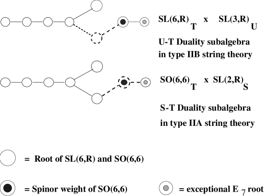
Figure 2.3:

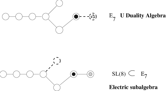
Figure 2.4:

From these embeddings occurring at the $E_{7}$ level, namely in $D=4$, one deduces the three embedding chains (2.27),(2.29),(2.30): it just suffices to peal off the last $\alpha_{r+1}$ roots one by one and also the $\beta$ root that occurs only in $D=4$. One observes that the appearance of the $\beta$ root is always responsible for an enhancement of the S–duality group. In the type IIA case this group is enhanced from $O(1,1)$ to $SL(2,{\rm I\kern-1.79993ptR})$ while in the type IIB case it is enhanced from the $SL(2,{\rm I\kern-1.79993ptR})_{U}$ already existing in $10$–dimensions to $SL(3,{\rm I\kern-1.79993ptR})$. Physically this occurs by combining the original dilaton field with the compactification radius of the latest compactified dimension.

2.4.3 String theory interpretation of the sequential embeddings: Type $IIA$, type $IIB$ and $M$ theory chains

We now turn to a closer analysis of the physical meaning of the embedding chains we have been illustrating.

Let us begin with the chain of eq.(2.29) that, as anticipated, is related with the type IIB interpretation of supergravity theory. The distinctive feature of this chain of embeddings is the presence of an addend $A_{1}$ that is already present in 10 dimensions. Indeed this $A_{1}$ is the Lie algebra of the $SL(2,R)_{\Sigma}$ symmetry of type $IIB$ D=10 superstring. We can name this group the U–duality symmetry $U_{10}$ in $D=10$. We can use the chain (2.29) to trace it in lower dimensions. Thus let us consider the decomposition

$$E_{r+1(r+1)} \rightarrow N_{r}\otimes SL(2,{\rm I\kern-1.79993ptR})$$

$$N_{r} = A_{r-1}\otimes O(1,1)$$ (2.42)

Obviously $N_{r}$ is not contained in the $T$-duality group $O(r,r)$ since the $NS$ tensor field $B_{\mu\nu}$ (which mixes with the metric under $T$-duality) and the $RR$–field $B^{c}_{\mu\nu}$ form a doublet with respect $SL(2,{\rm I\kern-1.79993ptR})_{U}$. In fact, $SL(2,{\rm I\kern-1.79993ptR})_{U}$ and $O(r,r)$ generate the whole U–duality group $E_{r+1(r+1)}$. The appropriate interpretation of the normaliser of $SL(2,R)_{\Sigma}$ in $E_{r+1(r+1)}$ is

$$N_{r}=O(1,1)\otimes SL(r,{\rm I\kern-1.79993ptR})\equiv GL(r,{\rm I\kern-1.79993ptR})$$ (2.43)

where $GL(r,{\rm I\kern-1.79993ptR})$ is the isometry group of the classical moduli space for the $T_{r}$ torus:

$$\frac{GL(r,{\rm I\kern-1.79993ptR})}{Or}.$$ (2.44)

The decomposition of the U–duality group appropriate for the type $IIB$ theory is

$$E_{r+1}\rightarrow U_{10}\otimes GL(r,{\rm I\kern-1.79993ptR})=SL(2,{\rm I\kern-1.79993ptR})_{U}\otimes O(1,1)\otimes SL(r,{\rm I\kern-1.79993ptR}).$$ (2.45)

Note that since $GL(r,{\rm I\kern-1.79993ptR})\supset O(1,1)^{r}$, this translates into $E_{r+1}\supset SL(2,{\rm I\kern-1.79993ptR})_{U}\otimes O(1,1)^{r}$. (In Type $IIA$, the corresponding chain would be $E_{r+1}\supset O(1,1)\otimes O(r,r)\supset O(1,1)^{r+1}$.) Note that while $SL(2,{\rm I\kern-1.79993ptR})$ mixes $RR$ and $NS$ states, $GL(r,{\rm I\kern-1.79993ptR})$ does not. Hence we can write the following decomposition for the solvable Lie algebra:

$$Solv_{r+1} = Solv\left(\frac{GL(r,{\rm I\kern-1.79993ptR})}{Or}\otimes\frac{SL(2,{\rm I\kern-1.79993ptR})}{O(2)}\right)+\left(\frac{\bf r(r-1)}{\bf 2},{\bf 2}\right)\oplus{\bf X}\oplus{\bf Y}$$

$$\mbox{dim }Solv_{r+1} = \frac{d(3d-1)}{2}+2+x+y.$$ (2.46)

where $x=\mbox{dim }{\bf X}$ counts the scalars coming from the internal part of the $4$–form $A^{+}_{{\mu}{\nu}{\rho}{\sigma}}$ of type IIB string theory. We have:

$$x=\left\{\matrix{0&r<4\cr\frac{r!}{4!(r-4)!}&r\geq 4\cr}\right.$$ (2.47)

and

$$y=\mbox{dim }{\bf Y}=\cases{\matrix{0&r<6\cr 2&r=6\cr}\cr}.$$ (2.48)

counts the scalars arising from dualising the two-index tensor fields in $r=6$.

For example, consider the $D=6$ case. Here the type $IIB$ decomposition is:

$$E_{5(5)}=\frac{O(5,5)}{O(5)\otimes O(5)}\rightarrow\frac{GL(4,{\rm I\kern-1.79993ptR})}{O(4)}\otimes\frac{SL(2,{\rm I\kern-1.79993ptR})}{O(2)}$$ (2.49)

whose compact counterpart is given by $O(10)\rightarrow SU(4)\otimes SU(2)\otimes U(1)$, corresponding to the decomposition: ${\bf 45}={\bf(15,1,1)}+{\bf(1,3,1)}+{\bf(1,1,1)}+{\bf(6,2,2)}+{\bf(1,1,2)}$. It follows:

$$Solv_{5}=Solv(\frac{GL(4,{\rm I\kern-1.79993ptR})}{O(4)}\otimes\frac{SL(2,{\rm I\kern-1.79993ptR})}{O(2)})+({\bf 6},{\bf 2})^{+}+({\bf 1},{\bf 1})^{+}.$$ (2.50)

where the factors on the right hand side parametrize the internal part of the metric $g_{ij}$, the dilaton and the $RR$ scalar ($\phi$, $\phi^{c}$), ($B_{ij}$, $B^{c}_{ij}$) and $A^{+}_{ijkl}$ respectively.

There is a connection between the decomposition (2.42) and the corresponding chains in M–theory. The type IIB chain is given by eq.(2.29), namely by

$$E_{r+1(r+1)}\rightarrow SL(2,{\rm I\kern-1.79993ptR})\otimes GL(r,{\rm I\kern-1.79993ptR})$$ (2.51)

while the $M$ theory is given by eq.(2.30), namely by

$$E_{r+1}\rightarrow O(1,1)\otimes SL(r+1,{\rm I\kern-1.79993ptR})$$ (2.52)

coming from the moduli space of $T^{11-D}=T^{r+1}$. We see that these decompositions involve the classical moduli spaces of $T^{r}$ and of $T^{r+1}$ respectively. Type $IIB$ and $M$ theory decompositions become identical if we decompose further $SL(r,{\rm I\kern-1.79993ptR})\rightarrow O(1,1)\times SL(r-1,{\rm I\kern-1.79993ptR})$ on the type $IIB$ side and $SL(r+1,{\rm I\kern-1.79993ptR})\rightarrow O(1,1)\otimes SL(2,{\rm I\kern-1.79993ptR})\otimes SL(r-1,{\rm I\kern-1.79993ptR})$ on the $M$-theory side. Then we obtain for both theories

$$E_{r+1}\rightarrow SL(2,{\rm I\kern-1.79993ptR})\times O(1,1)\otimes O(1,1)\otimes SL(r-1,{\rm I\kern-1.79993ptR}),$$ (2.53)

and we see that the group $SL(2,{\rm I\kern-1.79993ptR})_{U}$ of type $IIB$ is identified with the complex structure of the $2$-torus factor of the total compactification torus $T^{11-D}\rightarrow T^{2}\otimes T^{9-D}$.

Note that according to (2.41) in 8 and 4 dimensions, ($r=2$ and $6$) in the decomposition (2.53) there is the following enhancement (Figure 2.5):

$$SL(2,{\rm I\kern-1.79993ptR})\times O(1,1)\rightarrow SL(3,{\rm I\kern-1.79993ptR})\quad(\mbox{for}\,r=2,6)$$ (2.54)

$$\left\{\matrix{O(1,1)&\rightarrow&SL(2,{\rm I\kern-1.79993ptR})\quad(\mbox{for}\,r=2)\cr SL(5,{\rm I\kern-1.79993ptR})\times O(1,1)&\rightarrow&SL(6,{\rm I\kern-1.79993ptR})\quad(\mbox{for}\,r=6)\cr}\right.$$ (2.55)

Figure 2.5: Enhancement for type IIB in D=4 (r=6).

Finally, by looking at fig.((2.6)) let us observe that $E_{7(7)}$ admits also a subgroup $SL(2,{\rm I\kern-1.79993ptR})_{T}$ $\otimes(SO(5,5)_{S}$ $\equiv E_{5(5)})$ where the $SL(2,{\rm I\kern-1.79993ptR})$ factor is a T–duality group, while the factor $(SO(5,5)_{S}$ $\equiv E_{5(5)})$ is an S–duality group which mixes R–R and N–S states.

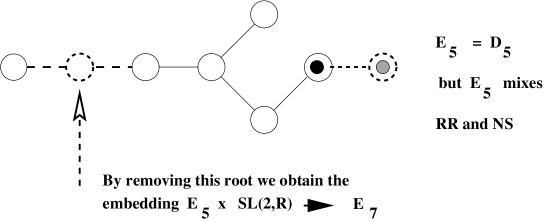
Figure 2.6:

2.5 The maximal abelian ideals ${\cal A}_{r+1}\subset Solv_{r+1}$ of the solvable Lie algebra

It is interesting to work out the maximal abelian ideals ${\cal A}_{r+1}\subset Solv_{r+1}$ of the solvable Lie algebras generating the scalar manifolds of maximal supergravity in dimension $D=10-r$. The maximal abelian ideal of a solvable Lie algebra is defined as the maximal subset of nilpotent generators commuting among themselves. From a physical point of view this is the largest abelian Lie algebra that one might expect to be able to gauge in the supergravity theory. Indeed, as it turns out, the number of vector fields in the theory is always larger or equal than $\mbox{dim}{\cal A}_{r+1}$. Actually, as we are going to see, the gaugeable maximal abelian algebra is always a proper subalgebra ${\cal A}^{gauge}_{r+1}\subset{\cal A}_{r+1}$ of this ideal.

The criteria to determine ${\cal A}^{gauge}_{r+1}$ will be discussed in the next section. In the present section we derive ${\cal A}_{r+1}$ and we explore its relation with the space of vector fields in one dimension above the dimension we each time consider. From such analysis we obtain a filtration of the solvable Lie algebra which provides us with a canonical polynomial parametrization of the supergravity scalar coset manifold $U_{r+1}/H_{r+1}$

2.5.1 The maximal abelian ideal from an algebraic viewpoint

Algebraically the maximal abelian ideal can be characterized by looking at the decomposition of the U–duality algebra $E_{r+1(r+1)}$ with respect to the U–duality algebra in one dimension above. In other words we have to consider the decomposition of $E_{r+1(r+1)}$ with respect to the subalgebra $E_{r(r)}\,\otimes\,O(1,1)$. This decomposition follows a general pattern which is given by the next formula:

$$\mbox{adj }E_{r+1(r+1)}\,=\,\mbox{adj }E_{r(r)}\,\oplus\,\mbox{adj }O(1,1)\,\oplus({\rm I\kern-1.79993ptD}^{+}_{r}\oplus{\rm I\kern-1.79993ptD}^{-}_{r})$$ (2.56)

where ${\rm I\kern-1.79993ptD}^{+}_{r}$ is at the same time an irreducible representation of the U–duality algebra $E_{r(r)}$ in $D+1$ dimensions and coincides with the maximal abelian ideal

$${\rm I\kern-1.79993ptD}^{+}_{r}\,\equiv\,{\cal A}_{r+1}\,\subset\,Solv_{(r+1)}$$ (2.57)

of the solvable Lie algebra we are looking for. In eq. (2.56) the subspace ${\rm I\kern-1.79993ptD}^{-}_{r}$ is just a second identical copy of the representation ${\rm I\kern-1.79993ptD}^{+}_{r}$ and it is made of negative rather than of positive weights of $E_{r(r)}$. Furthermore ${\rm I\kern-1.79993ptD}^{+}_{r}$ and ${\rm I\kern-1.79993ptD}^{-}_{r}$ correspond to the eigenspaces belonging respectively to the eigenvalues $\pm 1$ with respect to the adjoint action of the S–duality group $O(1,1)$.

2.5.2 The maximal abelian ideal from a physical perspective: the vector fields in one dimension above and translational symmetries

Here, we would like to show that the dimension of the abelian ideal in $D$ dimensions is equal to the number of vectors in dimensions $D+1$. Denoting the number of compactified dimensions by $r$ (in string theory, $r=10-D$), we will label the $U$-duality group in $D$ dimensions by $U_{D}=E_{11-D}=E_{r+1}$. The $T$-duality group is $O(r,r)$, while the $S$-duality group is $O(1,1)$ in dimensions higher than four, $SL(2,R)$ in $D=4$ (and it is inside $O(8,8)$ in $D=3$).

It follows from (2.56) that the total dimension of the abelian ideal is given by

$${\rm dim}\,{\cal A}_{D}\,\equiv\,{\rm dim}\,{\cal A}_{r+1}\,\equiv\,{\rm dim}\,{\rm I\kern-1.79993ptD}_{r}$$ (2.58)

where ${\rm I\kern-1.79993ptD}_{r}$ is a representation of $U_{D+1}$ pertaining to the vector fields. According to (2.56) we have (for $D\geq 4$):

$$\mbox{adj }U_{D}=\mbox{adj }U_{D+1}\oplus{\bf 1}\oplus({\bf 2},{\rm I\kern-1.79993ptD}_{r}).$$ (2.59)

This is just an immediate consequence of the embedding chain (2.26) which at the first level of iteration yields $E_{r+1}\rightarrow E_{r}\times O(1,1)$. For example, under $E_{7}\rightarrow E_{6}\times O(1,1)$ we have the branching rule: ${\rm adj}\,E_{7}={\rm adj}\,E_{6}+{\bf 1}+({\bf 2},{\bf 27})$ and the abelian ideal is given by the ${\bf 27^{+}}$ representation of the $E_{6(6)}$ group. The $70$ scalars of the $D=4,N=8$ theory are naturally decomposed as ${\bf 70}={\bf 42}+{\bf 1}+{\bf 27^{+}}$. To see the splitting of the abelian ideal scalars into $NS$ and $RR$ sectors, one has to consider the decomposition of $U_{D+1}$ under the T–duality group $T_{D+1}=O(r-1,r-1)$, namely the second iteration of the embedding chain (2.26): $E_{r+1}\rightarrow O(1,1)\times O(r-1,r-1)$. Then the vector representation of $O(r-1,r-1)$ gives the $NS$ sector, while the spinor representation yields the $RR$ sector. The example of $E_{7}$ considered above is somewhat exceptional, since we have ${\bf 27}\rightarrow({\bf 10}+{\bf 1}+{\bf 16})$. Here in addition to the expected ${\bf 10}$ and ${\bf 16}$ of $O(5,5)$ we find an extra $NS$ scalar: physically this is due to the fact that in four dimensions the two-index antisymmetric tensor field $B_{\mu\nu}$ is dual to a scalar, algebraically this generator is associated with the exceptional root $\sqrt{2}\epsilon_{7}$. To summarize, the $NS$ and $RR$ sectors are separately invariant under $O(r,r)$ in $D=10-r$ dimensions, while the abelian $NS$ and $RR$ sectors are invariant under $O(r-1,r-1)$. The standard parametrization of the $U_{D}/H_{D}$ and $U_{D+1}/H_{D+1}$ cosets gives a clear illustration of this fact:

$$\frac{U_{D}}{H_{D}}\sim(\frac{U_{D+1}}{H_{D+1}},r_{D+1},{\bf V}_{r}^{D+1}).$$ (2.60)

Here $r_{D+1}$ stands for the compactification radius, and ${\bf V}_{r}^{D+1}$ are the compactified vectors yielding the abelian ideal in $D$ dimensions.

Note that:

$$\mbox{adj}\,H_{D}=\mbox{adj}\,H_{D+1}\,+\,\mbox{adj}\,\mbox{Irrep}\,U_{D+1}$$ (2.61)

so it appears that the abelian ideal forms a representation not only of $U_{D+1}$ but also of the compact isotropy subgroup $H_{D+1}$ of the scalar coset manifold.

In the above $r=6$ example we find ${\rm adj}\,SU(8)={\rm adj}\,USp(8)\oplus{\bf 27^{-}}$, $\Longrightarrow$ ${\bf 63}={\bf 36}+{\bf 27^{-}}$.

2.5.3 Maximal abelian ideal and brane wrapping

Now we would like to turn to a uniform counting of the ideal dimension in diverse space–time dimensions. The fact that the ($D+1$)-dimensional vectors have $0$-branes as electric sources (or equivalently, ($D-3$)-branes as magnetic ones) reduces the analysis of the $RR$ sector to a simple exercise in counting the ways of wrapping higher dimensional $d$-branes around the cycles of the compact manifold. This procedure spares one from doing a case-by-case counting and worrying about the scalars arising from the dualization of the tensor fields. It also easily generalizes for manifolds other then $T^{r}$. The latter choice corresponds to the case of maximal preserved supersymmetry, for which the counting is presented here.

Starting from Type $IIA$ theory with 0, 2, 4, 6 -Dbranes [25], the total number of ($D+1$)-dimensional 0-Dbranes (i.e. the maximal abelian ideal in $D$–dimensions) is obtained by wrapping the Dbranes around the even cycles of the ($9-D$)-dimensional torus. One gets:

$$n_{{\cal A}}^{RR}=\sum_{k}b_{2k}(T^{9-D})=2^{8-D}$$ (2.62)

where $b_{2k}$ are the Betti numbers. The same result is obtained by counting the magnetic sources: in this case the sum is taken over alternating series of even (odd) cohomology for $9-D$ even (odd), since the $6$-Dbrane is wrapped on the $(9-D)$-dimensional cycle of $T^{9-D}$, the $4$-Dbrane on $(7-D)$-dimensional cycles and so on. Note that wrapping Dbranes around the cycles of the same dimensions as above but on a $T^{10-D}$ yields the total number of the $RR$ scalars in $D$ dimensions.

The type $IIB$ story is exactly the same with the even cycles replaced by the odd ones. The only little subtlety is in going from ten dimensions to nine - there is no $0$-Dbrane in type $IIB$, but instead there is a $RR$ scalar in the ideal already in ten dimensions, since the $U$-duality group is non-trivial. Of course the results agree on $T^{r}$ as they should on any manifold with a vanishing Euler number.

The $NS$ parts of the ideal ($(D-3)$-branes in ($D+1$)-dimensions) are obtained either by wrapping the ten-dimensional fivebrane or as magnetic sources for Kaluza-Klein vectors (note that for the $NS$ part, the reasonings for Type $IIA$ and $IIB$ are identical). The former are the fivebrane wrapped on $(8-D)$ cycles of $T^{9-D}$ (there are $(9-D)$ of them), while the latter are given by the same number since it is the number of the Kaluza–Klein vectors (number of $1$-cycles). Thus

$$n_{{\cal A}}^{NS}=2b_{1}(T^{9-D})=2(9-D).$$ (2.63)

The only exception to this formula is the $D=4$ case where, as discussed above, we have to add an extra scalar due to the $B_{\mu\nu}$ field.

2.6 Gauging

In this last section we will consider the problem of gauging some isometries of the coset $G/H$ in the framework of solvable Lie algebras.

In particular we will consider in more detail the gauging of maximal compact groups and the gauging of nilpotent abelian (translational) isometries.

This procedure is a way of obtaining partial supersymmetry breaking in extended supergravities [22],[26],[27] and it may find applications in the context of non perturbative phenomena in string and M-theories.

Let us consider the left–invariant 1–form $\Omega=L^{-1}dL$ of the coset manifold $U_{D}/H_{D}$, where $L$ is the coset representative.

The gauging procedure [28] amounts to the replacement of $dL$ with the gauge covariant differential $\nabla L$ in the definition of the left–invariant 1–form $\Omega=L^{-1}dL$:

$$\Omega\rightarrow\widehat{\Omega}=L^{-1}\nabla L=L^{-1}(d+A)L=\Omega+L^{-1}AL$$ (2.64)

As a consequence $\widehat{\Omega}$ is no more a flat connection, but its curvature is given by:

$$R(\widehat{\Omega})=d\widehat{\Omega}+\widehat{\Omega}\wedge\widehat{\Omega}=L^{-1}{\cal F}L\equiv L^{-1}(dA+A\wedge A)L=L^{-1}(F^{I}T_{I}+L^{I}_{AB}T_{I}\overline{\psi}^{A}\psi^{B})L$$ (2.65)

where $F^{I}$ is the gauged supercovariant 2–form and $T_{I}$ are the generators of the gauge group embedded in the U–duality representation of the vector fields.

Indeed, by very definition, under the full group $E_{r+1(r+1)}$ the gauge vectors are contained in the representation ${\rm I\kern-1.79993ptD}_{r+1}$. Yet, with respect to the gauge subgroup they must transform in the adjoint representation, so that ${\cal G}_{D}$ has to be chosen in such a way that:

$${\rm I\kern-1.79993ptD}_{r+1}\,\stackrel{{\scriptstyle{\cal G}_{D}}}{{\longrightarrow}}\,\mbox{adj}\,{\cal G}_{D}\,\oplus\,\mbox{rep}\,{\cal G}_{D}$$ (2.66)

where $\mbox{rep}\,{\cal G}_{D}$ is some other representation of ${\cal G}_{D}$ contained in the above decomposition.

It is important to remark that vectors which are in $\mbox{rep}{\cal G}_{D}$ (i.e. vectors which do not gauge ${\cal G}_{D}$) may be required, by consistence of the theory [31], to appear through their duals $(D-3)$–forms, as for instance happens for $D=5$ [29]. In an analogous way $p$–form potentials ($p\neq 1$) which are in non trivial representations of ${\cal G}_{D}$ may also be required to appear through their duals $(D-p-2)$–potentials, nas is the case in $D=7$ for $p=2$ [30].

The charges and the boosted structure constants discussed in the next subsection can be retrieved from the two terms appearing in the last expression of eq. (2.65)

2.6.1 Filtration of the $E_{r+1}$ root space, canonical parametrization of the coset representatives and boosted structure constants

As it has already been emphasized, the complete structure of $N>2$ supergravity in diverse dimensions is fully encoded in the local differential geometry of the scalar coset manifold $U_{D}/H_{D}$. All the couplings in the Lagrangian are described in terms of the metric, the connection and the coset representative (1.26) of $U_{D}/H_{D}$. A particularly significant consequence of extended supersymmetry is that the fermion masses and the scalar potential the theory can develop occur only as a consequence of the gauging and can be extracted from a decomposition in terms of irreducible $H_{D}$ representations of the boosted structure constants[86] [28]. Let us define these latter. Let ${\rm I\kern-1.79993ptD}_{r+1}$ be the irreducible representation of the $U_{D}$ U–duality group pertaining to the vector fields and denote by ${\vec{\bf w}}_{\Lambda}$ a basis for ${\rm I\kern-1.79993ptD}_{r+1}$:

$$\forall{\vec{\bf v}}\,\in\,{\rm I\kern-1.79993ptD}_{r+1}\qquad:\qquad{\vec{v}}\,=\,v^{\Lambda}\,{\vec{\bf w}}_{\Lambda}$$ (2.67)

In the case we consider of maximal supergravity theories, where the U–duality groups are given by $E_{r+1(r+1)}$ the basis vectors ${\vec{bfw}}_{\Lambda}$ can be identified with the $56$ weights of the fundamental $E_{7(7)}$ representation or with the subsets of this latter corresponding to the irreducible representations of its $E_{r+1(r+1)}$ subgroups, according to the branching rules:

$${\bf 56}{\stackrel{{\scriptstyle E_{6}}}{{\longrightarrow}}}\cases{{\bf 27+1}{\stackrel{{\scriptstyle E_{5}}}{{\longrightarrow}}}\cases{{\bf 16}{\stackrel{{\scriptstyle E_{4}}}{{\longrightarrow}}}{\bf\dots}\cr{\bf 10}{\stackrel{{\scriptstyle E_{4}}}{{\longrightarrow}}}{\bf\dots}\cr{\bf 1+1}{\stackrel{{\scriptstyle E_{4}}}{{\longrightarrow}}}{\bf\dots}\cr}\cr{\bf 27+1}{\stackrel{{\scriptstyle E_{5}}}{{\longrightarrow}}}\cases{{\bf 16}{\stackrel{{\scriptstyle E_{4}}}{{\longrightarrow}}}{\bf\dots}\cr{\bf 10}{\stackrel{{\scriptstyle E_{4}}}{{\longrightarrow}}}{\bf\dots}\cr{\bf 1+1}{\stackrel{{\scriptstyle E_{4}}}{{\longrightarrow}}}{\bf\dots}\cr}\cr}$$ (2.68)

Let:

$$<~{},~{}>\quad:\quad{\rm I\kern-1.79993ptD}_{r+1}\,\times{\rm I\kern-1.79993ptD}_{r+1}\,\longrightarrow\,{\rm I\kern-1.79993ptR}$$ (2.69)

denote the invariant scalar product in ${\rm I\kern-1.79993ptD}_{r+1}$ and let ${\vec{\bf w}}^{\Sigma}$ be a dual basis such that

$$<{\vec{\bf w}}^{\Sigma},{\vec{\bf w}}_{\Lambda}>\,=\,\delta^{\Sigma}_{\Lambda}$$ (2.70)

Consider then the ${\rm I\kern-1.79993ptD}_{r+1}$ representation of the coset representative (1.26):

$$L(\phi)\quad:\quad|{\vec{\bf w}}_{\Lambda}>\,\longrightarrow L(\phi)_{\Lambda}^{\Sigma}\,|{\vec{\bf w}}_{\Sigma}>,$$ (2.71)

and let $T^{I}$ be the generators of the gauge algebra ${\cal G}_{D}\,\subset E_{r+1(r+1)}$.

The only admitted generators are those with index $\Lambda=I\,\in\,{adj}\,{\cal G}_{D}$, and there are no gauge group generators with index $\Lambda\,\in\,\mbox{rep}\,{\cal G}_{D}$. Given these definitions the boosted structure constants are the following three–linear $3$–tensors in the coset representatives:

$$\,\hbox{$\vrule height=6.45831pt,width=0.4pt,depth=0.0pt\kern-3.00003pt{\rm C}$}_{\Sigma\Gamma}^{\Lambda}\left(\phi\right)\,\equiv\,\sum_{I=1}^{{\rm dim}{\cal G}_{D}}\,<{\vec{\bf w}}^{\Lambda}\,,\,L^{-1}\left(\phi\right)\,T_{I}\,L\left(\phi\right)\,{\vec{\bf w}}_{\Sigma}>\,<{\vec{\bf w}}^{I}\,,\,L\left(\phi\right){\vec{\bf w}}_{\Gamma}>$$ (2.72)

and by decomposing them into irreducible $H_{r+1}$ representations we obtain the building blocks utilized by supergravity in the fermion shifts, in the fermion mass–matrices and in the scalar potential.

In an analogous way, the charges appearing in the gauged covariant derivatives are given by the following general form:

$$Q_{I\Sigma}^{\Lambda}\,\equiv\,<{\vec{\bf w}}^{\Lambda}\,,\,L^{-1}\left(\phi\right)\,T_{I}\,L\left(\phi\right)\,{\vec{\bf w}}_{\Sigma}>$$ (2.73)

The coset representative $L\left(\phi\right)$ can be written in a canonical polynomial parametrization which should give a simplifying tool in mastering the scalar field dependence of all physical relevant quantities. This includes, besides mass matrices, fermion shifts and scalar potential, also the central charges [32].

The alluded parametrization is precisely what the solvable Lie algebra analysis produces.

To this effect let us decompose the solvable Lie algebra of $E_{7(7)}/SU(8)$ in a sequential way utilizing eq. (2.56). Indeed we can write the equation:

$$Solv_{7}={\cal C}_{7}\oplus\Phi^{+}(E_{7})$$ (2.74)

where $\Phi^{+}(E_{7})$ is the $63$ dimensional positive part of the $E_{7}$ root space. By repeatedly using eq. (2.56) we obtain:

$$\Phi^{+}(E_{7})=\Phi^{+}(E_{2})\oplus{\rm I\kern-1.79993ptD}^{+}_{2}\oplus{\rm I\kern-1.79993ptD}^{+}_{3}\oplus{\rm I\kern-1.79993ptD}^{+}_{4}\oplus{\rm I\kern-1.79993ptD}^{+}_{5}\oplus{\rm I\kern-1.79993ptD}^{+}_{6}$$ (2.75)

where $\Phi^{+}(E_{2})$ is the one–dimensional root space of the U–duality group in $D=9$ and ${\rm I\kern-1.79993ptD}^{+}_{r+1}$ are the weight-spaces of the $E_{r+1}$ irreducible representations to which the vector field in $D=10-r$ are assigned. Alternatively, as we have already explained, ${\cal A}_{r+2}\equiv{\rm I\kern-1.79993ptD}^{+}_{r+1}$ are the maximal abelian ideals of the U–duality group in $E_{r+2}$ in $D=10-r-1$ dimensions.

We can easily check that the dimensions sum appropriately as follows from:

$$\mbox{dim}\,\Phi^{+}(E_{7})\, = {63}$$

$$\mbox{dim}\,\Phi^{+}(E_{2})\, = {1}\quad\quad~{}\mbox{dim}\,{\rm I\kern-1.79993ptD}^{+}_{2}\,={3}$$

$$\mbox{dim}\,{\rm I\kern-1.79993ptD}^{+}_{3}\, = {6}\quad\quad~{}\mbox{dim}\,{\rm I\kern-1.79993ptD}^{+}_{4}\,={10}$$

$$\mbox{dim}\,{\rm I\kern-1.79993ptD}^{+}_{5}\, = {16}\quad\quad\mbox{dim}\,{\rm I\kern-1.79993ptD}^{+}_{4}\,={27}$$

Relying on eq. (2.74), (2.75) we can introduce a canonical set of scalar field variables:

$$\phi^{i} \longrightarrow Y_{i}\,\in{\cal C}\quad\quad i=1,\dots\,r$$

$$\tau^{i}_{k} \longrightarrow \,D^{(k)}_{i}\,\in{\rm I\kern-1.79993ptD}_{k}\quad i=1,\dots\,\mbox{dim }\,{\rm I\kern-1.79993ptD}_{k}\quad(k=2,\dots,6)$$

$$\tau_{1} \longrightarrow {\rm I\kern-1.79993ptD}_{1}\,\equiv\,E_{2}$$ (2.77)

and adopting the short hand notation:

$$\phi\cdot{\cal C} \equiv \phi^{i}\,Y_{i}$$

$$\tau_{k}\cdot{\rm I\kern-1.79993ptD}_{k} \equiv \tau^{i}_{k}\,D^{(k)}_{i}$$

we can write the coset representative for maximal supergravity in dimension $D=10-r$ as:

$$L = \exp\left[\phi\cdot{\cal C}\right]\,\prod_{k=1}^{r}\,\exp\left[\tau_{k}\cdot{\rm I\kern-1.79993ptD}_{k}\right]$$ (2.79)

$$= \prod_{j=1}^{r+1}S^{i}\,\prod_{k=1}^{r}\,\left({1}+\tau_{r}\cdot{\rm I\kern-1.79993ptD}_{r}\right)$$

The last line follows from the abelian nature of the ideals ${\rm I\kern-1.79993ptD}_{k}$ and from the position:

$$S^{i}\,\equiv\,\exp[\phi^{i}Y_{i}]$$ (2.80)

All entries of the matrix $L$ are therefore polynomials of order at most $2\,r\,+\,1$ in the $S^{i},\tau^{i}_{k},\tau_{1}$ “canonical” variables. Furthermore when the gauge group is chosen within the maximal abelian ideal it is evident from the definition of the boosted structure constants (2.72) that they do not depend on the scalar fields associated with the generators of the same ideal. In such gauging one has therefore a flat direction of the scalar potential for each generator of the maximal abelian ideal.

In the next section we turn to considering the possible gaugings more closely.

2.6.2 Gauging of compact and translational isometries

A necessary condition for the gauging of a subgroup ${\cal G}_{D}\subset U_{D}$ is that the representation of the vectors ${\rm I\kern-1.79993ptD}_{r+1}$ must contain $\mbox{adj}{\cal G}_{D}$. Following this prescription, the list of maximal compact gaugings ${\cal G}_{D}$ in any dimensions is obtained in the third column of Table 2.5. In the other columns we list the $U_{D}$-duality groups, their maximal compact subgroups and the left-over representations for vector fields.

Table 2.5: Maximal gauged compact groups

$D$	$U_{D}$	$H_{D}$	${\cal G}_{D}$	$\mbox{rep}{\cal G}_{D}$
9	$SL(2,{\rm I\kern-1.79993ptR})\times O(1,1)$	$O(2)$	$O(2)$	2
8	$SL(3,{\rm I\kern-1.79993ptR})\times SL(2,{\rm I\kern-1.79993ptR})$	$O(3)\times O(2)$	$O(3)$	$3$
7	$SL(5,{\rm I\kern-1.79993ptR})$	$USp(4)$	$O(5)\sim USp(4)$	0
6	$O(5,5)$	$USp(4)\times USp(4)$	$O(5)$	$5+1$
5	$E_{6,(6)}$	$USp(8)$	$O(6)\sim SU(4)$	$2\times 6$
4	$E_{7(7)}$	$SU(8)$	$O(8)$	0

Table 2.6: Transformation properties under ${\cal G}_{D}$ of 2- and 3-forms

$D$	$\mbox{rep}\,B_{\mu\nu}$	$\mbox{rep}\,A_{\mu\nu\rho}$
9	2	0
8	3	0
7	0	5
6	5	0
5	$2\times 6$	0

We notice that, for any $D$, there are $p$–forms ($p$ =1,2,3) which are charged under the gauge group ${\cal G}_{D}$. Consistency of these theories requires that such forms become massive. It is worthwhile to mention how this can occur in two variants of the Higgs mechanism. Let us define the (generalized) Higgs mechanism for a $p$–form mass generation through the absorption of a massless ($p-1$)–form (for $p=1$ this is the usual Higgs mechanism). The first variant is the anti-Higgs mechanism for a $p$–form [33], which is its absorption by a massless ($p+1$)–form. It is operating, for $p=1$, in $D=5,6,8,9$ for a sextet of $SU(4)$, a quintet of $SO(5)$, a triplet of $SO(3)$ and a doublet of $SO(2)$, respectively. The second variant is the self–Higgs mechanism [31], which only exists for $p=(D-1)/2$, $D=4k-1$. This is a massless $p$–form which acquires a mass through a topological mass term and therefore it becomes a massive “chiral” $p$–form. The latter phenomena was shown to occur in $D=3$ and $7$. It is amazing to notice that the representation assignments dictated by $U$–duality for the various $p$–forms is precisely that needed for consistency of the gauging procedure (see Table 2.6).

The other compact gaugings listed in Table 2.5 are the $D=4$ [34] and $D=8$ cases [35].

It is possible to extend the analysis of gauging semisimple groups also to the case of solvable Lie groups [16]. For the maximal abelian ideals of $Solv(U_{D}/H_{D})$ this amounts to gauge an $n$–dimensional subgroup of the translational symmetries under which at least $n$ vectors are inert. Indeed the vectors the set of vectors that can gauge an abelian algebra (being in its adjoint representation) must be neutral under the action of such an algebra. We find that in any dimension $D$ the dimension of this abelian group $\mbox{dim}{\cal G}_{abel}$ is given precisely by ${\rm dim}(\mbox{rep}{\cal G}_{D})$ which appear in the decomposition of ${\rm I\kern-1.79993ptD}_{r+1}$ under $O(r+1)$. We must stress that this criterium gives a necessary but not sufficient condition for the existence of the gauging of an abelian isometry group, consistent with supersymmetry.

Table 2.7: Decomposition of fields in representations of the compact group ${\cal G}_{D}=O(11-D)$

	vect. irrep	adj($O(11-D)$)	${\cal A}$	$\mbox{dim}{\cal G}_{abel}$
$D=9$	$1+2$	1	1	1
$D=8$	$3+3$	3	3	3
$D=7$	$6+4$	6	6	4
$D=6$	$10+5+1$	10	10	$5+1$
$D=5$	$15+6+6$	15	$15+1$	$6+6$
$D=4$	$(21+7)\times 2$	21	$21+1\times 6$	7

Chapter 3 Partial $N=2\rightarrow N=1$ SUSY Breaking

As it was previously anticipated, in the present chapter I will deal with the problem of partial $N=2\rightarrow N=1$ supersymmetry breaking within the general framework of $N=2$ supergravity coupled to an arbitrary number of vector multiplets and hypermultiplets and with arbitrary gauging of the scalar manifold isometries. In the following treatment I will mainly refer to a work by P. Fré, L. Girardello, I. Pesando and myself [16]. The relevance of this analysis to the logic of the present dissertation is to show how solvable Lie algebra machinery can be succesfully applied to a concrete supergravity problem, giving it a geometrical formulation and therefore simplifying considerably its solution. Indeed, describing the scalar sector of the theory in terms of algebraic objects allows to “visualize” geometrically the mechanism of partial supersymmetry breaking making it more intuitive. Moreover, applying the results discussed in last chapter, a physical meaning can be given to these geometrical objects, leading to a deeper understanding of the physics underlying the mechanism itself.

I shall start giving a brief introduction to the topic of partial supersymmetry breaking in the context of $N=2$ supersymmetric theories. $N=2$ supergravity and $N=2$ rigid gauge theory have recently played a major role in the discussion of string–string dualities [60, 44, 61, 62, 63, 64, 6] and in the analysis of the non–perturbative phases of Yang–Mills theories [65, 66, 67, 68]. Furthermore in its ten years long history, $N=2$ supergravity has attracted the interest of theorists because of the rich geometrical structure of its scalar sector, based on the manifold:

$${\cal M}_{scalar}={\cal SK}_{n}\,\otimes\,{\cal QM}_{m}$$ (3.1)

where ${\cal SK}_{n}$ denotes a complex $n$–dimensional special Kähler manifold [54, 69, 70, 71, 72] (for a review of Special Kähler geometry see either [73] or [74]) and ${\cal QM}_{m}$ a quaternionic $m$–dimensional quaternionic manifold, $n$ being the number of vector multiplets and $m$ the number of hypermultiplets [75, 76, 77, 71].

Unfortunately applications of $N=2$ supergravity to the description of the real world have been hampered by the presence of mirror fermions and by a tight structure which limits severely the mechanisms of spontaneous breaking of local $N=2$ SUSY. Any attempt to investigate the fermion problem requires a thorough understanding of the spontaneous breaking with zero vacuum energy. In particular, an interesting feature is the sequential breaking to $N=1$ and then to $N=0$ at two different scales.

As far as rigid supersymmetry is concerned, a well known theorem [111] forbids the possibility of partial supersymmetry breaking. A heuristic proof of this “no–go” theorem may be given in the following way. Consider the anti–commutation relation between N–extended supersymmetry generators $Q^{i}_{\alpha}\,;\,\,i=1,...,N$:

$$\{\overline{Q}^{i}_{\dot{\alpha}}\,,\,Q^{j}_{\alpha}\}\,=\,2\sigma_{{\dot{\alpha}}\alpha}^{\mu}\delta^{ij}P_{\mu}$$ (3.2)

where $P_{\mu}$ is the $4$–momentum generator. Computing the vacuum expectation value (vev) of both sides of the above equation, one gets the following expression for the vacuum energy:

$$E_{vac}\,=\,\frac{1}{2}\sum_{\alpha}\langle 0|Q^{\dagger i}_{\alpha}Q^{i}_{\alpha}|O\rangle\,=\,\frac{1}{2}\sum_{\alpha}||Q^{i}_{\alpha}|O\rangle||\,\,\,\,(\mbox{no summation over i})$$ (3.3)

If one supersymmetry, say $i=1$, is broken, one has that $Q^{1}_{\alpha}\,|O\rangle\neq 0$. This in turn implies, because of (3.3), that $E_{vac}\neq 0$ and therefore that all the supersymmetries are broken. This argument can be made rigorous [110] by considering the anti–commutation relation between local supercurrents in a theory formulated in finite volume and eventually performing the infinite volume limit. A way out from the “no–go” theorem was found in the rigid case by I. Antoniadis, H. Partouche and T.R. Taylor [83]. They considered an $N=2$ rigid theory with one vector multiplet and included in the lagrangian an electric and magnetic Fayet–Iliapulos term (APT model). This amounted to modifying the supercurrent version of (3.2) by means of an additive constant matrix on the right hand side, making the latter proportional to a non trivial $SU(2)$ matrix which could therefore have, on suitable vacua, one vanishing and one non vanishing eigenvalue.

On the local supersymmetry front, sometimes ago a negative result on partial breaking was established within the $N=2$ supergravity formulation based on conformal tensor calculus [78]. A particular way out was indicated in an ad hoc model [79] which prompted some generalizations based on Noether couplings [80].

With the developments in special Kähler geometry [55, 62, 63] stimulated by the studies on S–duality, the situation can now be cleared in general terms. Indeed it has appeared from [82, 83, 84, 85] that the negative results on $N=2$ partial supersymmetry breaking were the consequence of unnecessary restrictions imposed on the formulation of special Kähler geometry and could be removed. Moreover the minimal $N=2$ supergravity model ( coupled to one vector multiplet and one hypermultiplet) exhibiting partial supersymmetry breaking and introduced for the first time by S. Ferrara, L. Girardello and M. Porrati in [82], was shown to admit the APT model as a suitable flat limit.

As I anticipated at the beginning, in what follows the generic structure of partial supersymmetry breaking within the general form of $N=2$ supergravity coupled with $n+1$ vector multiplets and $m$ hypermultiplets will be discussed in detail. In particular an explicit example is worked out in section 3, based on the choice for the vector multiplets of the special Kähler manifold $SU(1,1)/U(1)\,\otimes\,SO(2,n)/SO(2)\times SO(n)$ and of the quaternionic manifold $SO(4,m)/SO(4)\times SO(m)$ for the hypermultiplets. In this section the mechanism of partial supersymmetry breaking is formulated mathematically by using the coset manifold description for ${\cal M}_{scalar}$. In section four the same result will be achieved by adopting the solvable Lie algebra description for both the Special Kähler and Quaternionic manifolds in (3.1) (Alekseevskii’s formalism) and it will be shown how this formulation of the problem, besides other advantages, allows to find, in a strightforward way, the flat directions of the scalar potential.

3.0.1 The bearing of the coordinate free definition of Special Kähler geometry

A main point in our subsequent discussion is the use of the symplectically covariant, coordinate free definition of special Kähler geometry (1.40) given in Chapter 1.

Consider an $n$ dimensinal Special Kähler manifold ${\cal SK}$ spanned by the scalar fields belonging to $n$ vector multiplets. Definition (1.40) of ${\cal SK}$ implies the existence of a correspondence $i_{\delta}$ between isometries on the base manifold ${\cal M}$ and $Sp(2n+2,{\rm I\kern-1.79993ptR})$ transformations on sections of the symplectic bundle ${\cal Z}\rightarrow{\cal M}$. These transformations turn out to be the same duality transformations mixing the electric field–strenghts $F^{\Lambda}$ with the magnetic ones $G_{\Sigma}$ which have been discussed in Capter 1 and $i_{\delta}$ is the embedding defined by (1.16). A change of basis for the symplectic sections of ${\cal Z}$ amounts to conjugating $i_{\delta}$ through a symplectic transformation $S$. It has been pointed out in Chapter 1 that such an operation is physically immaterial only if the theory is ungauged. As soon as an electric current is introduced the distinction is established and, at least at the classical (or semiclassical) level, the only symplectic transformations $S$ that yield equivalent theories (or can be symmetries) are the perturbative ones generated by lower triangular symplectic matrices:

$$\left(\matrix{{\bf A}&{\bf 0}\cr{\bf C}&{\bf D}\cr}\right)\,$$ (3.4)

It follows that different bases of symplectic sections for the bundle ${\cal Z}$ yield, after gauging, inequivalent physical theories. The possibility of realizing or not realizing partial supersymmetry breaking $N=2\,\rightarrow\,N=1$ are related to this choice of symplectic bases. In the tensor calculus formulation the lower part $F_{\Lambda}(z)$ of the symplectic section $\Omega(z)$ defined in (1.39) should be, necessarily, derivable from a holomorphic prepotential $F(X)$ that is a degree two homogeneous function of the upper half of the section:

$$F_{\Sigma}(z)=\frac{\partial}{\partial X^{\Sigma}(z)}\,F(X(z))\quad;\quad F\left(\lambda\,X^{\Sigma}(z)\,\right)=\,\lambda^{2}\,F\left(X^{\Sigma}(z)\,\right)$$ (3.5)

This additional request is optional in the more general geometric formulation of $N=2$ supergravity [71, 86] where only the intrinsic definition of special geometry is utilized for the construction of the lagrangian. It can be shown that the condition for the existence of the holomorphic prepotential $F(X)$ is the non degeneracy of the jacobian matrix $e^{I}_{i}(z)\equiv\partial_{i}\left(X^{I}/X^{0}\right);I=1,\dots,n$. There are symplectic bases where this jacobian has vanishing determinant and there no $F(X)$ can be found. If one insists on the existence of the prepotential such bases are discarded a priori.

There is however another criterion to select symplectic bases which has a much more intrinsic meaning and should guide our choice. Given the isometry group $G$ of the special Kähler manifold ${\cal SV}$, which is an intrinsic information, which subgroup of $G_{class}\subset G$ is realized by classical symplectic matrices $\left(\matrix{{\bf A}&{\bf 0}\cr{\bf 0}&{\bf D}\cr}\right)$ and which part of $G$ is realized by non perturbative symplectic matrices $\left(\matrix{{\bf A}&{\bf B}\cr{\bf C}&{\bf D}\cr}\right)$ with ${\bf B}\neq 0$ is a symplectic base dependent fact. It appears that in certain cases, very relevant for the analysis of string inspired supergravity, the maximization of $G_{class}$, required by a priori symmetry considerations, is incompatible with the condition ${\rm det}\left(e^{I}_{i}(z)\right)\,\neq\,0$ and hence with the existence of a prepotential $F(X)$. If the unneccessary condition on $F(X)$ existence is removed and the maximally symmetric symplectic bases are accepted the no-go results on partial supersymmetry breaking can also be removed. Indeed in [82] it was shown that by gauging a group

$$G_{gauge}={\rm I\kern-1.79993ptR}^{2}$$ (3.6)

in a N=2 supergravity model with just one vector multiplet and one hypermultiplet based on the scalar manifold:

$${\cal SK}=\frac{SU(1,1)}{U(1)}\quad\quad;\quad\quad{\cal Q}=\frac{SO(4,1)}{SO(4)}$$ (3.7)

supersymmetry can be spontaneously broken from $N=2$ down to $N=1$, provided one uses the symplectic basis where the embedding of $SU(1,1)\equiv SL(2,{\rm I\kern-1.79993ptR})$ in $Sp(4,{\rm I\kern-1.79993ptR})$ is the following :

$$\forall\,\left(\matrix{a&b\cr c&d\cr}\right)\,\in\,SL(2,{\rm I\kern-1.79993ptR})\quad{\stackrel{{\scriptstyle\i_{\delta}}}{{\hookrightarrow}}}\left(\matrix{a\,{\rm 1\kern-3.50006pt1}&b\,\eta\cr c\,\eta&d\,{\rm 1\kern-3.50006pt1}\cr}\right)\,\in\,Sp(4,{\rm I\kern-1.79993ptR})$$ (3.8)

Let us now turn on the general case of an $N=2$ supergravity with $n+1$ vector multiplets and $m$ hypermultiplets based on the scalar manifold:

$${\cal SK}_{n+1}=\frac{SU(1,1)}{U(1)}\otimes\frac{SO(2,n)}{SO(2)\otimes SO(n)}\quad\quad;\quad\quad{\cal QM}_{m}=\frac{SO(4,m)}{SO(4)\otimes SO(m)}$$ (3.9)

We show that we can obtain partial breaking $N=2\,\rightarrow\,N=1$ by

• choosing the Calabi–Vesentini symplectic basis where the embedding of $SL(2,{\rm I\kern-1.79993ptR})\otimes SO(2,n)$ into $Sp(4+2n,{\rm I\kern-1.79993ptR})$ is the following:

  $$\forall\,\left(\matrix{a&b\cr c&d\cr}\right)\,\in\,SL(2,{\rm I\kern-1.79993ptR}) {\stackrel{{\scriptstyle\i_{\delta}}}{{\hookrightarrow}}} \left(\matrix{a\,{\rm 1\kern-3.50006pt1}&b\,\eta\cr c\,\eta&d\,{\rm 1\kern-3.50006pt1}\cr}\right)\,\in\,Sp(2n+4,{\rm I\kern-1.79993ptR})$$

  $$\forall\,L\,\in\,SO(2,n) {\stackrel{{\scriptstyle\i_{\delta}}}{{\hookrightarrow}}} \left(\matrix{L&{\bf 0}\cr{\bf 0}&(L^{T})^{-1}\cr}\right)\,\in\,Sp(2n+4,{\rm I\kern-1.79993ptR})$$ (3.10)

  namely where all transformations of the group $SO(2,n)$ are linearly realized on electric fields

• gauging a group:

  $$G_{gauge}={\rm I\kern-1.79993ptR}^{2}\,\otimes\,G_{compact}$$ (3.11)

  where

  $${\rm I\kern-1.79993ptR}^{2}\, \cap SL(2,R)\otimes SO(2,n)=0$$

  $${\rm I\kern-1.79993ptR}^{2} \subset \mbox{ an abelian ideal of the solvable Lie subalgebra }V\,\subset so(4,m)$$

  $$G_{compact} \subset SO(n)\subset SO(2,n)$$

  $$G_{compact} \subset SO(m-1)\subset SO(4,m)$$ (3.12)

  namely where ${\rm I\kern-1.79993ptR}^{2}$ is a group of two abelian translations acting on the hypermultiplet manifold but with respect to which the vector multiplets have zero charge, while the compact gauge group $G_{compact}$ commutes with such translations and has a linear action on both the hypermultiplet and the vector multiplets.

In the following two sections I shall derive the result summarized above starting from the recently obtained complete form of N=2 supergravity with general scalar manifold interactions [86]. Let us conclude the present introduction with some physical arguments why the result should be obtained precisely in the way described above.

3.0.2 General features of the partial $N=2$ supersymmetry breaking

The mechanism of partial supersymmetry breaking that I am about to describe is referred to as super–Higgs mechanism and is “visually” represented in Figure 3.1.

Figure 3.1:

To break supersymmetry from $N=2$ down to $N=1$ we must break the $O(2)$ symmetry that rotates one gravitino into the other. This symmetry is gauged by the graviphoton $A^{0}_{\mu}$. Hence the graviphoton must become massive. At the same time, since we demand that $N=1$ supersymmetry should be preserved, the second gravitino must become the top state of an $N=1$ massive spin $3/2$ multiplet which has the form $\left\{\left({\o{3}{2}}\right),{2}\left(1\right),\left({\o{1}{2}}\right)\right\}$. Consequently not only the graviphoton but also a second gauge boson $A^{1}_{\mu}$ must become massive through ordinary Higgs mechanism. This explains while the partial supersymmetry breaking involves the gauging of a two–parameter group. That it should be a non compact ${\rm I\kern-1.79993ptR}^{2}$ acting as a translation group on the quaternionic manifold is more difficult to explain a priori, yet we can see why it is very natural. In order to obtain a Higgs mechanism for the graviphoton $A_{\mu}^{0}$ and the second photon $A_{\mu}^{1}$ these vectors must couple to the hypermultiplets. Hence these two fields should gauge isometries of the quaternionic manifold ${\cal QM}$. That such isometries should be translations is understood by observing that in this way one introduces a flat direction in the scalar potential, corresponding to the vacuum expectation value of the hypermultiplet scalar, coupled to the vectors in such a way. Finally the need to use the correct symplectic basis is explained by the following remark. Inspection of the gravitino mass-matrix shows that it depends on both the momentum map ${\cal P}^{0}_{\Lambda}(q)$ for the quaternionic action of the gauge group on the hypermultiplet manifold and on the upper (electric) part of the symplectic section $X^{\Lambda}(z)$. In order to obtain a mass matrix with a zero eigenvalue we need a contribution from both $X^{0}$ and $X^{1}$ at the breaking point, which can always be chosen at $z^{i}=0$, since the vector multiplet scalars are neutral (this is a consequence of ${\rm I\kern-1.79993ptR}^{2}$ being abelian). Hence in the correct symplectic basis we should have both $X^{0}(0)\neq 0$ and $X^{1}(0)\neq 0$. This is precisely what happens in the Calabi–Vesentini basis for the special Kähler manifold $SU(1,1)/U(1)\otimes SO(2,n)/SO(2)\otimes SO(n)$. Naming $y^{i}$ $(i=1,\dots,n)$ a standard set of complex coordinates for the $SO(2,n)/(SO(2)\otimes SO(n))$ coset manifold, characterized by linear transformation properties under the $SO(2)\otimes SO(n)$ subgroup and naming $S$ the dilaton field, i.e. the complex coordinate spanning the coset manifold $SU(1,1)/U(1)$, the explicit form of the symplectic section (1.39) corresponding to the symplectic embedding (3.10) is (see [55] and [73]):

$$\Omega\,=\,\left(\matrix{X^{0}\cr X^{1}\cr X^{i}\cr F_{0}\cr F_{1}\cr F_{i}\cr}\right)\,=\,\left(\matrix{\frac{1}{2}(1+y^{2})\cr\cr{\rm i}\frac{1}{2}(1-y^{2})\cr\cr y^{i}\cr S\,\frac{1}{2}(1+y^{2})\cr S\,{\rm i}\frac{1}{2}(1-y^{2})\cr-\,S\,y^{i}\cr}\right)\,{\stackrel{{\scriptstyle y\,\rightarrow\,0}}{{\longrightarrow}}}\,\left(\matrix{\frac{1}{2}\cr{\rm i}\frac{1}{2}\cr 0\cr\frac{1}{2}\,S\cr{\rm i}\frac{1}{2}\,S\cr 0\cr}\right)$$ (3.13)

3.1 Formulation of the $N=2\rightarrow N=1$ SUSY breaking problem

As it is well understood in very general terms (see [87]), a classical vacuum of an $N=r$ supergravity theory preserving $p\leq r$ supersymmetries in Minkowski space–time is just a constant scalar field configuration $\phi^{I}(x)=\phi^{I}_{0}\,(I=1,\dots,\mbox{dim}\,{\cal M}_{scalar})$ corresponding to an extremum of the scalar potential and such that it admits $p$ Killing spinors. In this context, Killing spinors are covariantly constant spinor parameters of the supersymmetry transformation $\eta^{A}_{(a)}$ $(A=1,\dots,n)$, $(a=1,\dots,p)$ such that the SUSY variation of the fermion fields in the bosonic background $g_{\mu\nu}=\eta_{\mu\nu}\,,\,A^{\Lambda}_{\mu}=0\,,\,\phi^{I}=\phi^{I}_{0}$ is zero for each $\eta^{A}_{(a)}$:

$$\delta_{a}\,\psi_{\mu A} \equiv {\rm i}\gamma_{\mu}\,S_{AB}(\phi_{0})\,\eta^{B}_{(a)}\,=\,0$$

$$\delta_{a}\xi^{i} \equiv \Sigma^{i}_{A}(\phi_{0})\,\eta^{A}_{(a)}\,=\,0\quad\quad(a=1,\dots,p)$$ (3.14)

In eq.( 3.14) the spin $3/2$ fermion shift $S_{AB}(\phi)$ and the spin $1/2$ fermion shifts $\Sigma^{i}_{A}(\phi)$ are the non-derivative contributions to the supersymmetry transformation rules of the gravitino $\psi_{\mu A}$ and of the spin one half fields $\xi^{i}$, respectively. The integrability conditions of supersymmetry transformation rules are just the field equations. So it actually happens that the existence of Killing spinors, as defined by eq.( 3.14), forces the constant configuration $\phi^{I}=\phi^{I}_{0}$ to be an extremum of the scalar potential.

Hence we can just concentrate on the problem of solving eq.( 3.14) in the case $N=2$ with $p=1$.

In $N=2$ supergravity there are two kinds of spin one half fields: the gauginos $\lambda^{j^{\star}}_{A}$ carrying an $SU(2)$ index $A=1,2$ and a world–index $j^{\star}=1^{\star},\dots,n^{\star}$ of the tangent bundle $T^{(0,1)}{\cal SK}$ to the special Kähler manifold ($n=\mbox{dim}_{\bf C}\,{\cal SK}=\#\mbox{vector multiplets}$ ) and the hyperinos $\zeta^{\alpha}$ carrying an index $\alpha$=$(1,\dots,n)$ running in the fundamental representation of $Sp(2m,{\rm I\kern-1.79993ptR})$ ($m=\mbox{dim}_{\bf Q}\,{\cal Q}=\#\mbox{hypermultiplets}$ ). Hence there are three kind of fermion shifts:

$$\delta\psi_{\mu A} = i\gamma_{\mu}S_{AB}\eta^{B}$$

$$\delta(g_{i^{*}j}\Lambda^{i^{*}}_{A}) = W_{j|AB}\eta^{B}$$

$$\delta\zeta^{\alpha} = N_{A}^{\alpha}\eta^{A}$$ (3.15)

According to the analysis and the conventions of [86, 71], the shifts are expressed in terms of the fundamental geometric structures defined over the special Kähler and quaternionic manifolds as follows:

$$S_{AB} = -\frac{1}{2}{\rm i}(\sigma_{x}\epsilon)_{AB}{\cal P}^{x}_{\Lambda}L^{\Lambda}$$

$$W_{j|AB} = -({\epsilon_{AB}}\partial_{j}{\cal P}_{\Lambda}L^{\Lambda}+{\rm i}(\sigma_{x}\epsilon)_{AB}{\cal P}^{x}_{\Lambda}f^{\Lambda}_{j})$$

$$N_{A}^{\alpha} = -2{\bf i}_{\vec{k}_{\Lambda}}{\cal U}^{\alpha}_{A}L^{\Lambda}\,=\,-2\,{\cal U}^{\alpha}_{A|u}\,k^{u}_{\Lambda}\,L^{\Lambda}$$ (3.16)

In eq.(3.16) the index $u$ runs on $4m$ values corresponding to any set of of $4m$ real coordinates for the quaternionic manifold. Further ${\cal P}_{\Lambda}$ is the holomorphic momentum map for the action of the gauge group ${\cal G}_{gauge}$ on the special Kähler manifold ${\cal SK}_{n}$, ${\cal P}^{x}_{\Lambda}\,(x=1,2,3)$ is the triholomorphic momentum map for the action of the same group on the quaternionic manifold, $L^{\Lambda}=e^{{\cal K}/2}X^{\Lambda}(z)$ is the upper part of the symplectic section (1.39), rescaled with the exponential of one half the Kähler potential ${\cal K}(z,{\overline{z}})$ (for more details on special geometry see [86], [73], [74]), ${\vec{k}}_{\Lambda}$ is the Killing vector generating the action of the gauge group on both scalar manifolds and finally ${\cal U}^{\alpha}_{A}$ is the vielbein 1–form on the quaternionic manifold carrying an $SU(2)$ doublet index and an index $\alpha$ running in the fundamental representation of $Sp(2m,{\rm I\kern-1.79993ptR})$.

In the case of effective supergravity theories that already take into account the perturbative and non–perturbative quantum corrections of string theory the manifolds ${\cal SK}$ and ${\cal Q}$ can be complicated non–homogeneous spaces without continuous isometries. It is not in such theories, however, that one performs the gauging of non abelian groups and that looks for a classical breaking of supersymmetry. Indeed, in order to gauge a non abelian group, the scalar manifold must admit that group as a group of isometries. Hence ${\cal M}_{scalar}$ is rather given by the homogeneous coset manifolds that emerge in the field theoretical limit to the tree level approximation of superstring theory. In a large variety of models the tree level approximation yields the choice ( 3.9) and we concentrate on such a case to show that a constant configuration with a single killing spinor can be found. Yet, as it will appear from our subsequent discussion, the key point of our construction resides in the existence of an ${\rm I\kern-1.79993ptR}^{2}$ translation isometry group on ${\cal Q}$ that can be gauged by two vectors associated with section components $X^{0}\,X^{1}$ that become constants in the vacuum configuration of ${\cal SK}$. That these requirements can be met is a consequence of the algebraic structure á la Alekseevski of both the special Kählerian and the quaternionic manifold. Since such algebraic structures exist for all homogeneous special and quaternionic manifolds, we are lead to conjecture that the partial supersymmetry breaking described below can be extended to most N=2 supergravity theories on homogenous scalar manifolds.

For the rest of the chapter, however, I shall concentrate on the study of case (3.9).

In the Calabi-Vesentini basis (3.13) the origin $y=0$ of the vector multiplet manifold $SO(2,n)/SO(2)\otimes SO(n)$ is a convenient point where to look for a configuration breaking $N=2\,\rightarrow\,N=1$. We shall argue that for $y=0$ and for an arbitrary point in the quaternionic manifold $\forall q\,\in\,SO(4,m)/SO(4)\times SO(m)$ there is always a suitable group ${\rm I\kern-1.79993ptR}^{2}_{q}$ whose gauging achieves the partial supersymmetry breaking. Actually the group ${\rm I\kern-1.79993ptR}^{2}_{q}$ is just the conjugate, via an element of the isometry group $SO(4,m)$, of the group ${\rm I\kern-1.79993ptR}^{2}_{0}$ the achieves the breaking in the origin $q=0$. Hence we can reduce the whole analysis to a study of the neighborhood of the origin in both scalar manifolds. To show these facts we need to cast a closer look at the structure of the hypermultiplet manifold.

3.2 Explicit solution

3.2.1 The quaternionic manifold $SO(4,m)/SO(4)\otimes SO(m)$

We start with the usual parametrization of the coset $SO(4,m)\over SO(4)\otimes SO(m)$ [88]:

$${\rm I\kern-1.79993ptL}(q)=\left(\matrix{\sqrt{1+qq^{t}}&q\cr q^{t}&\sqrt{1+q^{t}q}}\right)=\left(\matrix{r_{1}&q\cr q^{t}&r_{2}}\right)$$ (3.17)

where $q=||q_{at}||$ is a $4\times m$ matrix . This coset manifold has a riemannian structure defined by the vielbein, connection and metric given below :

$${\rm I\kern-1.79993ptL}^{-1}d{\rm I\kern-1.79993ptL} = \left(\matrix{\theta&E\cr E^{t}&\Delta}\right)\in so(4,m)$$

$$ds^{2} = E^{t}\otimes E$$ (3.18)

The explicit form of the vielbein and connections which we utilise in the sequel is:

$$E\,=\,r_{1}dq-qdr_{2}\quad;\quad\theta\,=\,r_{1}dr_{1}-qdq^{t}\quad;\quad\Delta\,=\,r_{2}dr_{2}-q^{t}dq$$ (3.19)

where $E$ is the coset vielbein, $\theta$ is the $so(4)$-connection and $\delta$ is the $so(n)$-connection. The quaternionic structure of the manifold is given by

$$K^{x}\,=\,\frac{1}{2}tr(E^{t}\wedge J^{x}E)\quad;\quad\omega^{x}\,=\,-\frac{1}{2}tr(\theta J^{x})\quad;\quad{\cal U}^{A\alpha}\,=\,\frac{1}{\sqrt{2}}E^{at}(e_{a})^{A}_{B}$$ (3.20)

$K^{x}$ being the triplet of hyperKähler 2–forms, $\omega^{x}$ the triplet of $su(2)$–connection 1–forms and ${\cal U}^{A\alpha}$ the vielbein 1–form in the symplectic notation. Furthermore $J^{x}$ is the triplet of $4\times 4$ self–dual ’t Hooft matrices $J^{+|x}$ normalized as in [86], $e_{a}$ are the quaternionic units as given in [86] and the symplectic index $\alpha=1,\dots,2m$ is identified with a pair of an $SU(2)$ doublet index $B=1,2$ times an $SO(4)$ vector index $t=1,\dots,m$: $\alpha\equiv Bt$. Notice also the factor $\frac{1}{2}$ in the definition of $K^{x}$ with respect to the conventions used in [86], which is necessary in order to have $\nabla\omega^{x}=-K^{x}$

3.2.2 Explicit action of the isometries on the coordinates and the killing vectors.

Next we compute the killing vectors; to this purpose we need to know the action of an element $g\in so(4,m)$ on the coordinates $q$. To this effect we make use of the standard formula

$$\delta{\rm I\kern-1.79993ptL}\equiv k^{at}_{g}\,\frac{\partial}{\partial q^{at}}=g{\rm I\kern-1.79993ptL}-{\rm I\kern-1.79993ptL}w_{g}$$ (3.21)

where

$$w_{g}=\left(\matrix{w_{1}&\cr&w_{2}}\right)\in so(4)\oplus so(m)$$ (3.22)

is the right compensator and the element $g\in so(4,m)$ is given by

$$g=\left(\matrix{a&b\cr b^{t}&c}\right)\in{\bf so(4,m)}$$ (3.23)

with $a^{t}=-a$, $c^{t}=-c$. The solution to (3.21) is:

$$\delta q=aq+br_{2}-qc-q\widehat{w}_{2} = aq+r_{1}b-qc+\widehat{w}_{1}q$$

$$\delta r_{1}=[a,r_{1}]+bq^{t}-r_{1}\widehat{w}_{1} \delta r_{2}=[c,r_{2}]+b^{t}q-r_{2}\widehat{w}_{2}$$ ;

$$w_{1}=a+\widehat{w}_{1} w_{2}=c+\widehat{w}_{2}$$ ; (3.24)

The only information we need to know about $\widehat{w}_{1},\widehat{w}_{2}$ is that they depend linearly on $b,b^{t}$. Anyhow for completess we give their explicit form:

$$\widehat{w}_{1;ab} = \left.{d(\sqrt{{\rm 1\kern-3.50006pt1}+x})_{ab}\over dx_{cd}}\right|_{x=qq^{t}}(bq^{t}-qb^{t})_{cd}$$

$$\widehat{w}_{2;st} = \left.{d(\sqrt{{\rm 1\kern-3.50006pt1}+y})_{st}\over dy_{pq}}\right|_{y=q^{t}q}(b^{t}q-q^{t}b)_{pq}$$ (3.25)

¿From these expressions we can obtain the Killing vector field

$$\vec{k}_{g}=(\delta q)_{at}\frac{\partial}{\partial q_{at}}$$ (3.26)

3.2.3 The momentum map.

We are now in a position to compute the triholomorphic momentum map ${\cal P}^{x}_{g}$ associated with the generic element 3.23 of the $so(4,m)$ Lie algebra. Given the vector field 3.26, we are supposed to solve the first order linear differential equation:

$${\bf i}_{{\vec{k}}_{g}}K^{x}=-\nabla{\cal P}^{x}$$ (3.27)

$\nabla$ denoting the exterior derivative covariant with respect to the $su(2)$–connection $\omega^{x}$ and ${\bf i}_{{\vec{k}}_{g}}K^{x}$ being the contraction of the 2–form $K^{x}$ along the Killing vector field ${\vec{k}}_{g}$. By direct verification the general solution is given by:

$${\cal P}^{x}_{g}=\frac{1}{2}tr(\left(\matrix{J^{x}&0\cr 0&0}\right)C_{g})=tr(J^{x}P_{g})$$ (3.28)

where for any element of the ${\bf so(4,m)}$ Lie algebra conjugated with the adjoint action of the coset representative (3.17), we have introduced the following block decomposition and notation:

$$\forall{g}\,\in\,{so(4,m)}:\quad C_{g}\,\equiv\,{\rm I\kern-1.79993ptL}(q)^{-1}g{\rm I\kern-1.79993ptL}(q)=\matrix{2P_{g}&{\bf i}_{\vec{k}}E_{g}\cr{\bf i}_{\vec{k}}E^{t}_{g}&2Q_{g}}$$ (3.29)

Furthermore if we decompose $g=g^{\Lambda}\,{\bf T}_{\Lambda}$ the generic element $g$ along a basis $\{{\bf T}_{\Lambda}\}$ of generators of the $so(4,m)$ Lie algebra, we can write:

$${\cal P}^{x}_{\Lambda}=\frac{1}{2}tr(\left(\matrix{J^{x}&0\cr 0&0}\right)C_{{\bf T}_{\Lambda}})=tr(J^{x}P_{{\bf T}_{\Lambda}})$$ (3.30)

3.2.4 Solution of the breaking problem in a generic point of the quaternionic manifold

At this stage we can attempt to find a solution for our problem i.e. introducing a gauging that yields a partial supersymmetry breaking.

Recalling the supersymmetry variations of the Fermi fields (3.15) we evaluate them at the origin of the special Kähler using the Calabi-Vesentini coordinates (3.13):

$$S_{AB}|_{y=0} = -{1\over 4}i(\sigma_{x}\epsilon)_{AB}tr(J^{x}(P_{0}+iP_{1}))$$

$$W_{s|AB}|_{y=0} = -{1\over 4(ImS)^{3\over 2}}i(\sigma_{x}\epsilon)_{AB}tr(J^{x}(P_{0}+iP_{1}))$$

$$W_{\alpha|AB}|_{y=0} = 0$$

$$N_{A}^{\alpha}|_{y=0} \propto ({\bf i}_{0}E^{at}-i{\bf i}_{1}E^{at}_{1})(e_{a})^{A}_{B}$$ (3.31)

where in the last equation we have identified $\alpha\equiv aB$ as explained after eq. (3.20).

In the next subsection we explicitly compute a solution for the matrices $P_{0},P_{1}$ and ${\bf i}_{0}E^{at},{\bf i}_{1}E^{at}$ at the origin of the quaternionic manifold ${\cal Q}_{m}$. Starting from this result it can be shown that any point $q\neq 0$ can define a vacuum of the theory in which SUSY is broken to $N=1$, provided a suitable gauging is performed. Indeed we can find the general solution for any point $q$ by requiring

$$C_{\Lambda}(q)=C_{\Lambda}(q=0)~{}~{}~{}~{}\Lambda=0,1$$ (3.32)

that is the group generators of the group we are gauging at a generic point $q$ are given by

$$T_{\Lambda}(q)={\rm I\kern-1.79993ptL}(q)T_{\Lambda}(0){\rm I\kern-1.79993ptL}^{-1}(q)$$ (3.33)

This result is very natural and just reflects the homogeneity of the coset manifold, i.e. all of its points are equivalent.

3.2.5 Solution of the problem at the origin of ${\cal Q}_{m}$.

In what follows all the earlier defined quantities, related to ${\cal Q}_{m}$, will be computed near the origin $q=0$. The right-hand side of equations (3.24,3.26) is expanded in powers of $q$ as it follows:

$$\delta q=b+aq-qc+O(q^{2}) \vec{k}_{a}\,=\,(aq)_{at}\frac{\partial}{\partial q_{at}}$$ ;

$$\vec{k}_{b}\,=\,b_{at}\frac{\partial}{\partial q_{at}} \vec{k}_{c}\,=\,-(qc)_{at}\frac{\partial}{\partial q_{at}}$$ ; (3.34)

The expressions for the vielbein, the connections and the quaternionic structure, to the approximation order we work, are:

$$E\,=\,dq-\frac{1}{2}qdq^{t}q \theta\,=\,\frac{1}{2}dqq^{t}-\frac{1}{2}qdq^{t}$$ ;

$$K^{x} = tr\left(dq^{t}~{}J^{x}~{}dq-dqq^{t}~{}J^{x}~{}dqq^{t}\right)$$

$$\omega^{x}\,=\,-\frac{1}{2}tr\left(dqq^{t}J^{x}\right) {\cal U}^{A\alpha}\,=\,\frac{1}{\sqrt{2}}dq^{at}(e_{a})^{A}_{B}$$ ; (3.35)

Finally the triholomorphic momentum maps corresponding to the a,b,c generators, have the following form, respectively :

$${\cal P}^{x}_{a}\,=\,\frac{1}{2}tr(J^{x}a+J^{x}qt^{t}a)\quad;\quad{\cal P}^{x}_{b}\,=\,-\frac{1}{2}tr(J^{x}qb^{t})\quad;\quad{\cal P}^{x}_{c}\,=\,-\frac{1}{2}tr(J^{x}qcq^{t})$$ (3.36)

Inserting eq.s (3.36) into equations (3.31) one finds the expressions for the shift matrices in the origin:

$$S_{AB}|_{y=0} = -{1\over 4}i(\sigma_{x}\epsilon)_{AB}tr(J^{x}(a_{0}+ia_{1}))$$

$$W_{s|AB}|_{y=0} = -{1\over 4(ImS)^{3\over 2}}i(\sigma_{x}\epsilon)_{AB}tr(J^{x}(a_{0}+ia_{1}))$$

$$W_{\alpha|AB}|_{y=0} = 0$$

$$N_{A}^{\alpha}|_{y=0} \propto (b_{0}^{at}-ib^{at}_{1})(e_{a})^{A}_{B}$$ (3.37)

$a_{0,1}$ and $b_{0,1}$ being the a and b blocks of the matrices $P_{0,1}$, respectively.

It is now clear that in order to break supersymmetry we need $a\neq 0$ and $b\neq 0$ . From the first two equations and from the requirement that the gravitino mass–matrix $S_{AB}$ should have a zero eigenvalue we get

$$\sum_{x}(a_{0}+ia_{1})^{2}_{x}=0\Rightarrow\vec{a}_{0}\cdot\vec{a}_{1}=(\vec{a}_{0})^{2}-(\vec{a}_{1})^{2}=0$$ (3.38)

We solve this constraint by setting ($a_{x}=-{1\over 4}tr(J^{x}a)$ )

$$a_{0x}=g_{0}\delta_{x1}~{}~{}~{}~{}a_{1x}=g_{1}\delta_{x2}$$ (3.39)

with $g_{0}=g_{1}$. These number are the gauge coupling constants of the repeatedly mentioned gauge group ${\rm I\kern-1.79993ptR}^{2}$. Note that due to the orthogonality of the antiself–dual t’Hooft matrices ${\overline{J}}^{x}$ to the self–dual ones $J^{x}$, the general solution is not as in eq. 3.39, but it involves additional arbitrary combinations of ${\overline{J}}^{x}$, namely:

$$a_{0}\,=\,g_{0}J^{1}+\overline{a}_{0x}\overline{J}^{x}\quad;\quad a_{1}\,=\,g_{1}J^{2}+\overline{a}_{1x}\overline{J}^{x}$$ (3.40)

For the conventions see [86]. To solve the last of eq.s (3.31) we set

$$b_{0}=\left(\matrix{0\cr\vec{\beta}_{0}\cr 0\cr 0}\right)~{}~{}~{}~{}b_{1}=\left(\matrix{0\cr 0\cr\vec{\beta}_{1}\cr 0}\right)$$ (3.41)

where $\vec{\beta}_{0}$ and $\vec{\beta}_{1}$ are $m$–vectors of the in the fundamental representation of $SO(m)$.

Now the essential questions are:

1. Can one find two commuting matrices belonging to the ${\bf so(4,m)}$ Lie algebra and satisfying the previous constraints? These matrices are the generators of ${\rm I\kern-1.79993ptR}^{2}$.

2. If so, which is the maximal compact subalgebra ${\bf G}_{compact}\subset{\bf so(4,m)}$ commuting with them, namely the maximal compact subalgebra of the centralizer $Z({\rm I\kern-1.79993ptR}^{2})$? ${\bf G}_{compact}$ is the Lie algebra of the maximal compact gauge group that can survive unbroken after the partial supersymmetry breaking.

Let $a_{2},b_{2},c_{2}$ denote the blocks of the commutator $[g_{0},g_{1}]$. To answer the first question we begin to seek a solution with $c=0$, and it is easily checked that also their commutator have vanishing block $c_{3}$. Let us now look at the condition $a_{2}=0$, namely

$$a_{2}=[a_{0},a_{1}]+b_{0}b_{1}^{t}-b_{1}b_{0}^{t}=2g_{0}g_{1}J^{3}+2\epsilon^{xyz}\overline{a}_{0}^{x}\overline{a}_{1}^{y}\overline{J}^{z}+\frac{1}{2}\vec{\beta}_{0}\cdot\vec{\beta}_{1}(J^{3}+\overline{J}^{3})=0$$ (3.42)

This equation can be solved if we set

$$\overline{a}_{0}^{x}\,=\,\gamma g_{0}\delta_{x1}\quad;\quad\overline{a}_{1}^{x}\,=\,\gamma g_{1}\delta_{x2}\quad;\quad\vec{\beta}_{0}\cdot\vec{\beta}_{1}=-4g_{0}g_{1}$$ (3.43)

and if $\gamma^{2}=1\,\leftarrow\,\gamma=\pm 1$. Now we are left to solve the equation $b_{2}=a_{0}b_{1}-a_{1}b_{0}=0$, which implies

$$(\gamma-1)g_{0}\vec{b}_{1}=(\gamma-1)g_{1}\vec{b}_{0}$$ (3.44)

This equation is automatically fulfilled if $\gamma=1$ for any choice of the $\vec{b}_{i}$s, while it is not consistent with the last of equations (3.43) if $\gamma=-1$. Thus the only admissible value for $\gamma$ is $1$.

Choosing $\vec{\beta}_{0}=(\beta_{0},0\dots 0)$ we can immediately answer the second question: for the normalizer of the ${\rm I\kern-1.79993ptR}^{2}$ algebra we have $Z_{\bf so(4,m)}\left({\rm I\kern-1.79993ptR}^{2}\right)={\bf so(m-1)}$, so that of the $m$ hypermultiplets one is eaten by the superHiggs mechanism and the remaining $m-1$ can be assigned to any linear representation of a compact gauge group that can be as large as $SO(m-1)$.

3.3 The $N=2\rightarrow N=1$ breaking problem in Alekseevskiǐ’s formalism.

There are two main motivations for the choice of Alekseevskiǐ’s formalism [19],[40] while dealing with the partial breaking of $N=2$ supersymmetry:

• it provides a description of the quaternionic manifold as a group manifold on which the generators of the ${\rm I\kern-1.79993ptR}^{2}$ act as traslation operators on two (say $t_{0},t_{1}$) of the $4m$ scalar fields, parametrizing ${\cal Q}_{m}$;

• as it will be apparent in the sequel, the fields $t_{0},t_{1}$ define flat directions for the scalar potential. They can be identified with the hidden sector of the theory, for their coupling to the gauge fields $A_{\mu}^{0}$ and $A_{\mu}^{1}$ is what determines the partial supersymmetry breaking.

Thus Alekseevskiǐ’s description of quaternionic manifolds provides a conceptually very powerful tool to deal with the SUSY breaking problem, even in the case in which ${\cal QM}$ is not a symmetric homogeneous manifold [89]. In what follows I will refer to the Alekseevskiǐ’s description of quaternionic manifolds introduced in Chapter 1, specializing it to the symmetric manifold ${\cal QM}_{m}$, and in terms of its $4m$–dimensional quaternionic algebra $V_{m}$, an explicit realization of the gauge group generators will be found.

3.3.1 The Quaternionic Algebra and Partial SUSY Breaking.

Alekseevskiǐ’s description of $V_{m}$ is given by (1.48), (1.49) and (1.50). The Kählerian algebra $W_{m}$ corresponding to $V_{m}$ through the C–map has the general structure illustrated in (LABEL:Wstru) in which the subspaces X and Y have dimension zero:

$$W_{m}\,=\,F_{1}\oplus F_{2}\oplus F_{3}\oplus Z\,\,;\,\,Z\,=\,Z^{+}\oplus Z^{-}$$ (3.45)

The $m-4$–dimensional spaces $Z^{\pm}$ and its image $\widetilde{Z}^{\pm}$ through $J_{2}$ in $\widetilde{U}$ are the only parts of the whole algebra whose dimension depends on $m=\#~{}of~{}hypermultiplets$, and thus it is natural to choose the fields parametrizing them in some representation of ${\cal G}_{compact}$, for, as it was shown earlier, ${\cal G}_{compact}\subset SO(m-1)$. At fixed $m$ the $Z$-sector can provide enough scalar fields as to fill a representation of the compact gauge group. On the other hand the fields of the hidden sector are to be chosen in the orthogonal complement with respect to $Z$ and $\widetilde{Z}$ and to be singlets with respect to ${\cal G}_{compact}$. Indeed, by definition the fields of the hidden sector interact only with $A_{\mu}^{0}$ and $A_{\mu}^{1}$

Using Alekseevskiǐ’s notation, an orthonormal basis for the U subspace of $V_{m}$ is provided by $\{h_{i},g_{i}\quad(i=0,1,2,3),z^{\pm}_{k}(k=1,...,m-4)\}$, while for $\widetilde{U}$ an orthonormal basis is given by $\{p_{i},q_{i}\quad(i=0,1,2,3),\widetilde{z}^{\pm}_{k}\quad(k=1,...,m-4)\}$. The elements $\{h_{i},g_{i},p_{i},q_{i}\quad(i=0,1,2,3)\}$ generate the maximally non–compact subalgebra $O(4,4)/O(4)\times O(4)$ of $V_{m}$ which is characteristic of the large class of quaternionic manifolds we are considering and which include also the $E_{6(2)}/SU(2)\times U(6)$ manifold to be studied in more detail in next chapter.

All these generators have a simple representation in terms of the canonical basis of the full isometry algebra ${\bf so(4,m)}$.

The next step is to determine within this formalism, the generators of the gauge group. As far as the ${\rm I\kern-1.79993ptR}^{2}$ factor is concerned we demand it to act by means of translations on the coordinates of the coset representative ${\rm I\kern-1.79993ptL}(q)$. To attain this purpose the generators of the translations $T_{0},T_{1}$ will be chosen within an abelian ideal ${\cal A}\subset V_{m}$ and the representative of ${\cal QM}_{m}$ will be defined in the following way:

$${\rm I\kern-1.79993ptL}(t,b)\,=\,e^{T(t)}e^{G(b)}\quad(t) = t^{0},t^{1}\quad;\quad(b)=b^{1},...,b^{4m-2}$$

$$T(t)\,=\,t^{\Lambda}T_{\Lambda}\quad\Lambda=0,1 G(t)\,=\,b^{a}G_{i}\quad a=1,...,4m-2$$ ;

$$V_{m} = T\oplus G$$ (3.46)

It is apparent from eq.(3.46) that the left action of a transformation generated by $T_{\Lambda}$ amounts to a translation of the coordinates $t^{0},t^{1}$. The latter will define flat directions for the scalar potential. As the scalar potential depends on the quaternionic coordinates only through ${\cal P}^{x}_{\alpha}$ and the corresponding killing vector, to prove the truth of the above statement it suffices to show that the momentum-map ${\cal P}^{x}_{\alpha}(t,b)$ on ${\cal QM}_{m}$ does not depend on the variables $t^{\Lambda}$. Indeed a general expression for ${\cal P}^{x}_{\alpha}$ associated to the generator $T_{\alpha}$ of ${\bf so(4,m)}$ is given by equation (3.28):

$${\cal P}^{x}_{\alpha}(t,b)=\frac{1}{2}tr({\rm I\kern-1.79993ptL}^{-1}(t,b)T_{\alpha}{\rm I\kern-1.79993ptL}(t,b){\cal J}^{x})=\frac{1}{2}tr(e^{-G}e^{-T}T_{\alpha}e^{T}e^{G}{\cal J}^{x})$$ (3.47)

If $T_{\alpha}$ is a generator of the gauge group, then either it is in $T$ or it is in the compact subalgebra. In both cases it commutes with $T$ allowing the exponentials of $T(t)$ to cancel against each other. It is also straightforward to prove that the Killing vector components on ${\cal QM}_{m}$ do not depend on $t^{\Lambda}$.

A maximal abelian ideal ${\cal A}$ in $V_{m}$ can be shown to have dimension $m+2$. Choosing

$${\cal A}=\left\{e_{1},g_{3},p_{0},p_{3},q_{1},q_{2},\widetilde{z}_{+}^{k}\right\}\quad\quad(k=1,...,m-4)$$ (3.48)

one can show that possible candidates for the role of translation generators are either $T_{\Lambda}$ or $T^{\prime}_{\Lambda}$ defined below:

$$T_{0} = e_{1}-g_{3}=E_{\epsilon_{l}+\epsilon_{3}}-E_{\epsilon_{1}-\epsilon_{3}},\quad T_{1}=p_{0}-p_{3}=E_{\epsilon_{1}-\epsilon_{3}}-E_{\epsilon_{1}+\epsilon_{3}}$$

$$T^{\prime}_{0} = p_{0}-p_{3}=E_{\epsilon_{1}-\epsilon_{3}}-E_{\epsilon_{1}+\epsilon_{3}}\,,\,T^{\prime}_{1}=q_{2}-q_{1}=E_{\epsilon_{1}+\epsilon_{4}}-E_{\epsilon_{1}-\epsilon_{4}}$$ (3.49)

where $\epsilon_{k},\quad k=1,...,l=\mbox{rank}({\bf so(4,m)})$ is an orthonormal basis of ${\rm I\kern-1.79993ptR}^{l}$ and $\epsilon_{i}\pm\epsilon_{j}$ are roots of $so(4,m)$. In the previous section we found constraints on the form of the ${\rm I\kern-1.79993ptR}^{2}$ generators in order for partial SUSY breaking to occur on a vacuum defined at the origin of ${\cal QM}_{m}$. The matrices $T_{\Lambda}$ fulfill such requirements. On the other hand one can check that also $T^{\prime}_{\Lambda}$ fit the purpose as well, even if they do not have the form predicted in the previous section.Indeed specializing the fermion shift matrices in (3.16) to a background defined by $y=0\,;\,b=0$ one finds:

$$W^{\overline{s}}_{AB}\, \propto \,(\sigma^{x}\epsilon^{-1})_{AB}({\cal P}^{x}_{0}+{\rm i}{\cal P}^{x}_{1})$$

$$W^{\overline{\alpha}}_{AB}\, \propto \,(\sigma^{x}\epsilon^{-1})_{AB}{\cal P}^{x}_{\overline{\alpha}}$$

$$S_{AB}\, \propto \,(\sigma^{x}\epsilon^{-1})_{AB}({\cal P}^{x}_{0}+{\rm i}{\cal P}^{x}_{1})$$

$$N^{A}_{\alpha}\, \propto \,(\epsilon e^{a}\epsilon^{-1})^{A}_{B}(g_{0}{\cal U}^{a|t}_{0}-{\rm i}g_{1}{\cal U}^{a|t}_{1})$$

where:

$$e^{0} = Id_{2\times 2}\,\,;\,\,e^{x}=-i\sigma^{x}\,\,\alpha=(t,B)=1,...,2m$$ (3.50)

Gauging for instance $T_{\Lambda}$ as generators of ${\rm I\kern-1.79993ptR}^{2}$, from (3.47) it follows that

$${\cal P}^{x}_{0}\, = \,-g_{0}\delta^{x}_{3}\,\,;\,\,{\cal P}^{x}_{1}\,=\,g_{1}\delta^{x}_{2}\,\,;\,\,{\cal P}^{x}_{\overline{\alpha}}\,=\,0$$

$${\cal U}^{2|t}_{0}\, = \,2\,\,;\,\,{\cal U}^{3|t}_{1}\,=\,-2$$

$$\matrix{S_{AB}\cr W^{\overline{s}}_{AB}}\, \propto \,\left(\matrix{g_{1}&g_{0}\cr g_{0}&g_{1}}\right)$$

$$W^{\overline{\alpha}}_{AB}\, = \,0$$ (3.51)

Setting $g_{0}=g_{1}$ the shift matrices in (3.51) have the following killing spinor: $\eta^{A}=(1,-1)$. Computing the gaugino shift matrices one finds that $\eta^{A}N_{A}\propto(g_{0}-g_{1})$ which vanishes for $g_{0}=g_{1}$.

Moreover, taking $T_{\Lambda}$ as generators of ${\rm I\kern-1.79993ptR}^{2}$, it follows from their matrix form that the largest compact subalgebra of ${\bf so(4,m)}$ suitable for generating ${\cal G}_{compact}$ is ${\bf so(m-1)}$.

As it was also pointed out in the previous section, any point on ${\cal QM}_{m}$ described by $q=(t,b)$ can define a vacuum on which SUSY is partially broken, provided that a suitable choice for the isometry generators to be gauged is done, e.g.:

$$T_{\alpha}(t,b)={\rm I\kern-1.79993ptL}(t,b)T_{\alpha}{\rm I\kern-1.79993ptL}(t,b)^{-1}$$ (3.52)

To this extent all the points on the surface spanned by $t^{0},t^{1}$ and containing the origin, require the same kind of gauging (as it is apparent from equation (3.52)), and this is another way of justifying the flatness of the scalar potential along these two directions.

The existence of a Killing spinor guarantees that on the corresponding constant scalar field configuration $N=2$ SUSY is broken to $N=1$, and the scalar potential vanishes. Furthermore, as explained in [87] and already recalled, the existence of at least one Killing spinor implies the stability of the background,namely that it is an extremum of the scalar potential. We have explicitly verified that the configuration $(y=0;b=0)$ are minima of the scalar potential by plotting its projection on planes, corresponding to different choices of pairs $(y,b)$ of coordinates which were let to vary while keeping all the others to zero. The behaviour of all these curves shows a minimum in the origin, where the potential vanishes, as expected. Two very typical representatives of the general behaviour of such plots are shown in figure 1 and 2.

Figure 3.2: Scalar Potential Vs y generic and b coefficient of $e_{0}$

Figure 3.3: Scalar Potential Vs y generic and b coefficient of $h_{1}$.

Chapter 4 BPS Black Holes in Supergravity

In this last chapter I want to consider the application of solvable Lie algebras to the derivation of the differential equations that characterize BPS states as classical supergravity solutions. The main reference for the present discussion is a recent paper by L. Andrianopoli, R. D’Auria, S.Ferrara, P. Fré and myself [109].

Interest in the extremal black hole solutions of $D=4$ supergravity theories has been quite vivid in the last couple of years [10, 91] and it is just part of a more general interest in the $p$–brane classical solutions of supergravity theories in all dimensions $4\leq D\leq 11$ [92, 93]. This interest streams from the interpretation of the classical solutions of supergravity that preserve a fraction of the original supersymmetries as the BPS non perturbative states necessary to complete the perturbative string spectrum and make it invariant under the conjectured duality symmetries discussed in the first chapters. This identification has become quite circumstantial with the advent of $D$–branes [25] and the possibility raised by them of a direct construction of the BPS states within the language of perturbative string theory extended by the choice of Dirichlet boundary conditions [25].

4.0.1 BPS–saturated states in supergravity: extremal Black Holes

From an abstract viewpoint BPS saturated states are characterized by the fact that they preserve, in modern parlance, $1/2$ (or $1/4$, or $1/8$) of the original supersymmetries. What this actually means is that there is a suitable projection operator ${\rm I\kern-1.79993ptP}^{2}_{BPS}={\rm I\kern-1.79993ptP}_{BPS}$ acting on the supersymmetry charge $Q_{SUSY}$, such that:

$$\left({\rm I\kern-1.79993ptP}_{BPS}\,Q_{SUSY}\right)\,|\,\mbox{BPS state}\,>\,=\,0$$ (4.1)

Since the supersymmetry transformation rules of any supersymmetric field theory are linear in the first derivatives of the fields eq.(4.1) is actually a system of first order differential equations. This system has to be combined with the second order field equations of supergravity and the common solutions to both system of equations is a classical BPS saturated state. That it is actually an exact state of non–perturbative string theory follows from supersymmetry representation theory. The classical BPS state is by definition an element of a short supermultiplet and, if supersymmetry is unbroken, it cannot be renormalized to a long supermultiplet.

Translating eq. (4.1) into an explicit first order differential system requires knowledge of the supersymmetry transformation rules of supergravity and it is at this level that solvable Lie algebras can play an important role. In order to grasp the significance of the above statement let us first rapidly review, as an example, the algebraic definition of $D=4$, $N=2\nu$ BPS states and then the idea of the solvable Lie algebra representation of the scalar sector.

The $D=4$ supersymmetry algebra with an even number $N=2\nu$ of supersymmetry charges can be written in the following form:

$$\left\{{\overline{Q}}_{aI|\alpha}\,,\,{\overline{Q}}_{bJ|\beta}\right\}\,=\,{\rm i}\left(C\,\gamma^{\mu}\right)_{\alpha\beta}\,P_{\mu}\,\delta_{ab}\,\delta_{IJ}\,-\,C_{\alpha\beta}\,\epsilon_{ab}\,\times\,\mathchoice{\hbox{\cmss Z\kern-3.99994ptZ}}{\hbox{\cmss Z\kern-3.99994ptZ}}{\lower 0.9pt\hbox{\cmsss Z\kern-2.79996ptZ}}{\lower 1.2pt\hbox{\cmsss Z\kern-2.79996ptZ}}_{IJ}$$

$$\left(a,b=1,2\qquad;\qquad I,J=1,\dots,\nu\right)$$ (4.2)

where the SUSY charges ${\overline{Q}}_{aI}\equiv Q_{aI}^{\dagger}\gamma_{0}=Q^{T}_{ai}\,C$ are Majorana spinors, $C$ is the charge conjugation matrix, $P_{\mu}$ is the 4–momentum operator, $\epsilon_{ab}$ is the two–dimensional Levi Civita symbol and the symmetric tensor $\mathchoice{\hbox{\cmss Z\kern-3.99994ptZ}}{\hbox{\cmss Z\kern-3.99994ptZ}}{\lower 0.9pt\hbox{\cmsss Z\kern-2.79996ptZ}}{\lower 1.2pt\hbox{\cmsss Z\kern-2.79996ptZ}}_{IJ}=\mathchoice{\hbox{\cmss Z\kern-3.99994ptZ}}{\hbox{\cmss Z\kern-3.99994ptZ}}{\lower 0.9pt\hbox{\cmsss Z\kern-2.79996ptZ}}{\lower 1.2pt\hbox{\cmsss Z\kern-2.79996ptZ}}_{JI}$ is the central charge operator. It can always be diagonalized $\mathchoice{\hbox{\cmss Z\kern-3.99994ptZ}}{\hbox{\cmss Z\kern-3.99994ptZ}}{\lower 0.9pt\hbox{\cmsss Z\kern-2.79996ptZ}}{\lower 1.2pt\hbox{\cmsss Z\kern-2.79996ptZ}}_{IJ}=\delta_{IJ}\,Z_{J}$ and its $\nu$ eigenvalues $Z_{J}$ are the central charges.

The Bogomolny bound on the mass of a generalized monopole state:

$$M\,\geq\,|\,Z_{I}|\qquad\forall Z_{I}\,,\,I=1,\dots,\nu$$ (4.3)

is an elementary consequence of the supersymmetry algebra and of the identification between central charges and topological charges. To see this it is convenient to introduce the following reduced supercharges:

$${\overline{S}}^{\pm}_{aI|\alpha}=\frac{1}{2}\,\left({\overline{Q}}_{aI}\gamma_{0}\pm\mbox{i}\,\epsilon_{ab}\,{\overline{Q}}_{bI}\,\right)_{\alpha}$$ (4.4)

They can be regarded as the result of applying a projection operator to the supersymmetry charges:

$${\overline{S}}^{\pm}_{aI} = {\overline{Q}}_{bI}\,{\rm I\kern-1.79993ptP}^{\pm}_{ba}$$

$${\rm I\kern-1.79993ptP}^{\pm}_{ba} = \frac{1}{2}\,\left({\bf 1}\delta_{ba}\pm\mbox{i}\epsilon_{ba}\gamma_{0}\right)$$ (4.5)

Combining eq.(4.2) with the definition (4.4) and choosing the rest frame where the four momentum is $P_{\mu}$ =$(M,0,0,0)$, we obtain the algebra:

$$\left\{{\overline{S}}^{\pm}_{aI}\,,\,{\overline{S}}^{\pm}_{bJ}\right\}=\pm\epsilon_{ac}\,C\,{\rm I\kern-1.79993ptP}^{\pm}_{cb}\,\left(M\mp Z_{I}\right)\,\delta_{IJ}$$ (4.6)

By positivity of the operator $\left\{{S}^{\pm}_{aI}\,,\,{\overline{S}}^{\pm}_{bJ}\right\}$ it follows that on a generic state the Bogomolny bound (4.3) is fulfilled. Furthermore it also follows that the states which saturate the bounds:

$$\left(M\pm Z_{I}\right)\,|\mbox{BPS state,}i\rangle=0$$ (4.7)

are those which are annihilated by the corresponding reduced supercharges:

$${\overline{S}}^{\pm}_{aI}\,|\mbox{BPS state,}i\rangle=0$$ (4.8)

On one hand eq.(4.8) defines short multiplet representations of the original algebra (4.2) in the following sense: one constructs a linear representation of (4.2) where all states are identically annihilated by the operators ${\overline{S}}^{\pm}_{aI}$ for $I=1,\dots,n_{max}$. If $n_{max}=1$ we have the minimum shortening, if $n_{max}=\nu$ we have the maximum shortening. On the other hand eq.(4.8) can be translated into a first order differential equation on the bosonic fields of supergravity. Indeed, let us consider a configuration where all the fermionic fields are zero. Setting the fermionic SUSY rules appropriate to such a background equal to zero we find the following Killing spinor equation:

$$0=\delta\mbox{fermions}=\mbox{SUSY rule}\left(\mbox{bosons},\epsilon_{AI}\right)$$ (4.9)

where the SUSY parameter satisfies the following conditions:

$$\begin{array}[]{rclcl}\xi^{\mu}\,\gamma_{\mu}\,\epsilon_{aI}&=&\mbox{\rm i}\,\varepsilon_{ab}\,\epsilon^{bI}&;&I=1,\dots,n_{max}\\ \epsilon_{aI}&=&0&;&I>n_{max}\\ \end{array}$$ (4.10)

Here $\xi^{\mu}$ is a time-like Killing vector for the space-time metric and $\epsilon_{aI},\epsilon^{aI}$ denote the two chiral projections of a single Majorana spinor:

$$\gamma_{5}\,\epsilon_{aI}\,=\,\epsilon_{aI}\quad;\quad\gamma_{5}\,\epsilon^{aI}\,=-\epsilon^{aI}$$ (4.11)

Eq.(4.9) has two features which we want to stress as main motivations for the developments presented in later sections:

1. It requires an efficient parametrization of the scalar field sector

2. It breaks the original $SU(2\nu)$ automorphism of the supersymmetry algebra to the subgroup $SU(2)\times SU(2\nu-2)\times U(1)$

The first feature is the reason why the use of the solvable Lie algebra $Solv$ associated with $U/SU(2\nu)\times H^{\prime}$ is of great help in this problem. The second feature is the reason why the solvable Lie algebra $Solv$ has to be decomposed in a way appropriate to the decomposition of the isotropy group $H=SU(2\nu)\times H^{\prime}$ with respect to the subgroup $SU(2)\times SU(2\nu-2)\times U(1)\times H^{\prime}$.

Before continuing our analysis it is worth giving, in this introductory section, a sketchy overview of some aspects of extremal Black Hole solutions in supergravity. Black Holes are classical solutions of Einstein–Maxwell equations whose space–time structure is asimptotically flat and has a singularity hidden by an event horizon. As it is well known, supergravity, being invariant under local super–Poincaré transformations, includes General Relativity, i.e. describes gravitation coupled to other fields in a supersymmetric framework. In particular, among its classical solutions there are Black Holes.

We are interested in BPS saturated states among the charged, stationary, asymptotically flat, spherically symmetric solutions. They are described by a particular kind of Black Holes which have a solitonic interpretation. Indeed their configurations turn out to interpolate between two vacuum states of the theory (as one expects from a soliton): the trivial Minkowski flat metric at spatial infinity and the Bertotti–Robinson conformally–flat metric near the horizon. When no scalar fields are coupled to gravity, this solution reduces to an extreme Reissner–Nordström configuration described by the following metric:

$$ds^{2}\,=\,\left(1-\frac{|q|}{r}\right)^{2}dt^{2}\,-\,\left(1-\frac{|q|}{r}\right)^{-2}dr^{2}-r^{2}d\Omega^{2}$$ (4.12)

being $r$ the radial distance from the singularity $r=0$, $d\Omega^{2}$ the solid angle element and $q$ the electric charge of the Black Hole which, in the chosen units, equals its ADM mass: $M=|q|$. This solution has a unique horizon defined as the sphere on which $g_{tt}=0$, i.e. whose radius is $r_{o}=|q|$. Changing the radial variable $r\rightarrow\rho=r-r_{o}$, equation (4.12) is rewritten in the following way:

$$ds^{2}\,=\,\left(1+\frac{|q|}{\rho}\right)^{-2}dt^{2}\,-\,\left(1+\frac{|q|}{\rho}\right)^{2}\left(d\rho^{2}+\rho^{2}d\Omega^{2}\right)$$ (4.13)

This solution has an apparent flat limit for $\rho\rightarrow\infty$ and near the horizon $\rho\approx 0$ eq. (4.13) reduces to:

$$ds^{2}\,=\,\frac{\rho^{2}}{M_{BR}^{2}}dt^{2}\,-\,\frac{M_{BR}^{2}}{\rho^{2}}\left(d\rho^{2}+\rho^{2}d\Omega^{2}\right)$$ (4.14)

which is the Bertotti–Robinson metric ($M_{BR}$ is the Bertotti–Robinson mass which equals, for this particular solution, the ADM mass i.e. $M_{BR}=|q|$).

When gravity is coupled with scalar fields $\phi$ the BPS saturated solution is more complicate as we will see. The boundary conditions on the sphere at infinity are defined by a flat Minkowsky metric and a constant value of the scalars $\phi(S^{2}_{\infty})\equiv\phi_{0}$ corresponding to a point on the moduli space of the theory. The BPS condition (4.7) on the ADM mass of the solution may be rewritten in the following way:

$$M_{ADM}\,=\,|Z_{I}(p,q,\phi_{0})|\,\,\,\,I=1,...,n_{max}$$ (4.15)

This condition is then translated in a system of first order differential equations derived from (4.9) in the bosonic fields. It has been shown two years ago, [107], [108] that the scalar solution to this system plus the equations of motion, describes a path in the moduli space along which the scalars are driven to a fixed point $\phi\rightarrow\phi_{fix}$ corresponding to the horizon of the Black Hole. In other words, near the horizon, the scalars “loose memory” of their initial values on $S^{2}_{\infty}$. The values of the scalars at the fixed point depend, as we are going to see later, only on the ratios of the electric and magnetic charges $q,p$ of the Black Hole measured on $S^{2}_{\infty}$ and are defined by minimizing $Z_{I}(p,q,\phi)$ with respect to the scalars $\phi$. In the proximity of the horizon, the metric is again the Bertotti–Robinson one, but this time $M_{BR}$ turns out to be equal to the value of the central charge $M_{BR}=|Z_{min}(p,q,\phi_{fix}(p,q))|/4\pi$ at the horizon, i.e. its minimum with respect to the scalar fields.

Bekenstein–Hawking formula relates the entropy of a Black Hole to the area of its horizon. Applying it to our solution, one obtains:

$$S\,=\,\frac{A}{4\pi}\,=\,\frac{1}{4\pi}\int_{horizon}d\theta d\phi\sqrt{g_{\theta\theta}g_{\phi\phi}}\,=\,M_{BR}^{2}\,=\,\frac{|Z_{min}(p,q)|^{2}}{4\pi}$$ (4.16)

where we used the Bertotti–Robinson metric to compute the area of the horizon. Since $Z_{min}$ and therefore the entropy does not depend on the values of the scalars at infinity $\phi_{0}$, they can be expressed in terms of moduli–independent topological quantities $I$ depending only on the U–duality group and on the representation of the electric and magnetic charges and defined on the whole moduli space [112]. As far as the $N=8$, $D=4$ theory is concerned, we know that the U–duality group is $E_{7(7)}$ which has a quartic invariant $I_{4}$. Since $I_{4}$ depends only on the charge vector of the Black Hole, in order for it to be non–zero (i.e. in order for the Black Hole to have a non–vanishing entropy), it can be shown that the solution should have at least four charges. This is the kind of solutions that we are going to study in what follows.

4.0.2 N=2 decomposition in the $N=8$ theory

In the present chapter I shall concentrate on the maximally extended four–dimensional theory, namely $N=8$ supergravity. In Chapter 2 we studied in detail some important properties of the scalar manifold $E_{7(7)}/SU(8)$ of this theory, by analysing its generating solvable Lie algebra denoted by $Solv_{7}$. According to the previous discussion the Killing spinor equation for $N=8$ BPS states requires that $Solv_{7}$ should be decomposed according to the decomposition of the isotropy subgroup: $SU(8)\longrightarrow SU(2)\times U(6)$. We show in later sections that the corresponding decomposition of the solvable Lie algebra is the following one:

$$Solv_{7}=Solv_{3}\,\oplus\,Solv_{4}$$ (4.17)

$$\begin{array}[]{rclrcl}Solv_{3}&\equiv&Solv\left(SO^{\star}(12)/U(6)\right)&Solv_{4}&\equiv&Solv\left(E_{6(2)}/SU(2)\times SU(6)\right)\\ \mbox{rank }\,Solv_{3}&=&3&\mbox{rank }\,Solv_{4}&=&4\\ \mbox{dim }\,Solv_{3}&=&30&\mbox{dim }\,Solv_{4}&=&40\\ \end{array}$$ (4.18)

In the present chapter I shall slightly change the notation introduced in Chapter 2, and denote by $Solv_{3}$ and $Solv_{4}$ non maximally–non–compact solvable algebras. The rank three Lie algebra $Solv_{3}$ defined above describes the thirty dimensional scalar sector of $N=6$ supergravity, while the rank four solvable Lie algebra $Solv_{4}$ contains the remaining fourty scalars belonging to $N=6$ spin $3/2$ multiplets. It should be noted that, individually, both manifolds $\exp\left[Solv_{3}\right]$ and $\exp\left[Solv_{4}\right]$ have also an $N=2$ interpretation since we have:

$$\exp\left[Solv_{3}\right] =$$ homogeneous special Kähler

$$\exp\left[Solv_{4}\right] =$$ homogeneous quaternionic (4.19)

so that the first manifold can describe the interaction of $15$ vector multiplets, while the second can describe the interaction of $10$ hypermultiplets. Indeed if we decompose the $N=8$ graviton multiplet in $N=2$ representations we find:

$$\mbox{N=8}\,\mbox{\bf spin 2}\,\stackrel{{\scriptstyle N=2}}{{\longrightarrow}}\,\mbox{\bf spin 2}+6\times\mbox{\bf spin 3/2}+15\times\mbox{\bf vect. mult.}+10\times\mbox{\bf hypermult.}$$ (4.20)

Although at the level of linearized representations of supersymmetry we can just delete the $6$ spin $3/2$ multiplets and obtain a perfectly viable $N=2$ field content, at the full interaction level this truncation is not consistent. Indeed, in order to get a consistent $N=2$ truncation the complete scalar manifold must be the direct product of a special Kähler manifold with a quaternionic manifold. This is not true in our case since putting together $\exp\left[Solv_{3}\right]$ with $\exp\left[Solv_{4}\right]$ we reobtain the $N=8$ scalar manifold $E_{7(7)}/SU(8)$ which is neither a direct product nor Kählerian, nor quaternionic. The blame for this can be put on the decomposition (4.17) which is a direct sum of vector spaces but not a direct sum of Lie algebras: in other words we have

$$\left[Solv_{3}\,,\,Solv_{4}\right]\,\neq\,0$$ (4.21)

The problem of deriving consistent $N=2$ truncations is most efficiently addressed in the language of Alekseveeskian solvable algebras [19]. $Solv_{3}$ is a Kähler solvable Lie algebra, while $Solv_{4}$ is a quaternionic solvable Lie algebra. We must determine a Kähler subalgebra ${\cal K}\,\subset\,Solv_{3}$ and a quaternionic subalgebra ${\cal Q}\,\subset\,Solv_{4}$ in such a way that:

$$\left[{\cal K}\,,\,{\cal Q}\right]\,=\,0$$ (4.22)

Then the truncation to the vector multiplets described by ${\cal K}$ and the hypermultiplets described by ${\cal Q}$ is consistent at the interaction level. An obvious solution is to take no vector multiplets ( ${\cal K}=0$) and all hypermultiplets ( ${\cal Q}=Solv_{4}$) or viceversa ( ${\cal K}=Solv_{3}$), ( ${\cal Q}=0$). Less obvious is what happens if we introduce just one hypermultiplet, corresponding to the minimal one–dimensional quaternionic algebra. In later sections we show that in that case the maximal number of admitted vector multiplets is $9$. The corresponding Kähler subalgebra is of rank 3 and it is given by:

$$Solv_{3}\,\supset\,{\cal K}_{3}\,\equiv\,Solv\left(SU(3,3)/SU(3)\times U(3)\right)$$ (4.23)

Note that, as we will discuss in the following, the 18 scalars parametrizing the manifold $SU(3,3)/SU(3)\times U(3)$ are all the scalars in the NS-NS sector of $SO^{*}(12)$. A thoroughful discussion of the N=2 truncation problem and of its solution in terms of solvable Lie algebra decompositions is discussed in section 4.5.1. At the level of the present introductory section we want to stress the relation of the decomposition (4.17) with the Killing spinor equation for BPS black-holes.

Indeed, as just pointed out, the decomposition (4.17) is implied by the $SU(2)\times U(6)$ covariance of the Killing spinor equation. As we show in section (3.2) this equation splits into various components corresponding to different $SU(2)\times U(6)$ irreducible representations. Introducing the decomposition (4.17) we will find that the $40$ scalars belonging to $Solv_{4}$ are constants independent of the radial variable $r$. Only the $30$ scalars in the Kähler algebra $Solv_{3}$ can have a radial dependence. In fact their radial dependence is governed by a first order differential equation that can be extracted from a suitable component of the Killing spinor equation. In this way we see that the same solvable Lie algebra decompositions occurring in the problem of N=2 truncations of N=8 supergravity occur also in the problem of constructing N=8 BPS black holes.

We present now our plan for the next sections.

In section 4.1 we discuss the structure of the scalar sector in $N=8$ supergravity and its supersymmetry transformation rules. As just stated, our goal is to develop methods for the analysis of BPS states as classical solutions of supergravity theories in all dimensions and for all values of $N$. Many results exist in the literature for the $N=2$ case in four dimensions [9, 94, 95], where the number of complex scalar fields involved just equals the number of differential equations one obtains from the Killing spinor condition. Our choice to focus on the $N=8$, $D=4$ case is motivated by the different group–theoretical structure of the Killing spinor equation in this case and by the fact that it is the maximally extended supersymmetric theory.

In section 4.2 we introduce the black–hole ansatz and we show how using roots and weights of the $E_{7(7)}$ Lie algebra we can rewrite in a very intrinsic way the Killing spinor equation. We analyse its components corresponding to irreducible representations of the isotropy subalgebra $U(1)\times SU(2)\times SU(6)$ and we show the main result, namely that the $40$ scalars in the $Solv_{4}$ subalgebra are constants.

In section 4.3 we exemplify our method by explicitly solving the simplified model where the only non–zero fields are the dilatons in the Cartan subalgebra. In this way we retrieve the known $a$–model solutions of N=8 supergravity.

The following two sections 5 and 4.5 are concerned with the method and the results of our computer aided calculations on the embedding of the subalgebras $U(1)\times SU(2)\times SU(6)\subset SU(8)$ in $E_{7(7)}$ and with the structure of the solvable Lie algebra decomposition already introduced in eq.(4.17). In particular we study the problem of consistent N=2 truncations using Alekseevski formalism. These two sections, being rather technical, can be skipped in a first reading by the non interested reader. We note however that many of the results there obtained are used for the discussion of the subsequent section. In particular, these results are preliminary for the allied project of gauging the maximal gaugeable abelian ideal ${\cal G}_{abel}$, which I have outlined in the previous chapters and which is still work in progress. Note that such a gauging should on one hand produce spontaneous partial breaking of $N=8$ supersymmetry and on the other hand be interpretable as due to the condensation of $N=8$ BPS black-holes.

In the final section 4.6 we address the question of the most general BPS black-hole. Using the little group of the charge vector in its normal form which, following [97], is identified with $SO(4,4)$, we are able to conclude that the only relevant scalar fields are those associated with the solvable Lie subalgebra:

$$Solv\left(\frac{SL(2,{\rm I\kern-1.79993ptR})^{3}}{U(1)^{3}}\right)\,\subset\,Solv_{3}$$ (4.24)

where the 6 scalars that parametrize the manifold $\frac{SL(2,{\rm I\kern-1.25995ptR})^{3}}{U(1)^{3}}$ are all in the NS-NS sector.

Moreover, with an appropriate identification, we show how the calculation of the fixed scalars performed by the authors of [96] in the N=2 STU model amounts to a solution of the same problem also in the N=8 theory. The most general solution can be actually generated by U-duality rotations of $E_{7(7)}$.

Therefore, the final result of our whole analysis, summarized in the conclusions is that up to U-duality transformations the most general $N=8$ black-hole is actually an $N=2$ black-hole corresponding however to a very specific choice of the special Kähler manifold, namely $\frac{SO^{*}(12)}{U(6)}$ as in eq.(4.18), (4.19).

4.1 N=8 Supergravity and its scalar manifold $E_{7(7)}/SU(8)$

The bosonic Lagrangian of $N=8$ supergravity contains, besides the metric $28$ vector fields and $70$ scalar fields spanning the $E_{7(7)}/SU(8)$ coset manifold. This lagrangian falls into the general type of lagrangians admitting electric–magnetic duality rotations considered in [86],[73],[55]. For the case where all the scalar fields of the coset manifold have been switched on the Lagrangian, according to the normalizations of [86] has the form:

$${\cal L}=\sqrt{-g}\,\left(2\,R[g]+\frac{1}{4}\,\mbox{Im}\,{\cal N}_{\Lambda\Sigma}\,{\cal F}^{\Lambda|\mu\nu}\,{\cal F}^{\Sigma}_{\mu\nu}+\frac{1}{4}\mbox{Re}\,{\cal N}_{\Lambda\Sigma}\,{\cal F}^{\Lambda}_{\mu\nu}\,{\cal F}^{\Sigma}_{\rho\sigma}\,\epsilon^{\mu\nu\rho\sigma}+\frac{\alpha^{2}}{2}\,g_{ij}(\phi)\,\partial_{\mu}\phi^{i}\,\partial^{\mu}\phi^{j}\right)$$ (4.25)

where the indeces $\Lambda,\Sigma$ enumerate the $28$ vector fields, $g_{ij}$ is the $E_{7(7)}$ invariant metric on the scalar coset manifold, $\alpha$ is a real number fixed by supersymmetry and the period matrix ${\cal N}_{\Lambda\Sigma}$ has the following general expression holding true for all symplectically embedded coset manifolds [38]:

$${\cal N}_{\Lambda\Sigma}=h\cdot f^{-1}$$ (4.26)

The complex $28\times 28$ matrices $f,h$ are defined by the $Usp(56)$ realization ${\rm I\kern-1.79993ptL}_{Usp}\left(\phi\right)$ of the coset representative which is related to its $Sp(56,{\rm I\kern-1.79993ptR})$ counterpart ${\rm I\kern-1.79993ptL}_{Sp}(\phi)$ through a Cayley transformation, as dispayed in the following formula [32]:

$${\rm I\kern-1.79993ptL}_{Usp}\left(\phi\right) = \frac{1}{\sqrt{2}}\left(\matrix{f+{\rm i}h&\overline{f}+{\rm i}\overline{h}\cr f-{\rm i}h&\overline{f}-{\rm i}\overline{h}\cr}\right)$$

$$\equiv {\cal C}\,{\rm I\kern-1.79993ptL}_{Sp}\left(\phi\right){\cal C}^{-1}$$

$${\rm I\kern-1.79993ptL}_{Sp}(\phi) \equiv \exp\left[\phi^{i}\,T_{i}\right]\,=\,\left(\matrix{A(\phi)&B(\phi)\cr C(\phi)&D(\phi)\cr}\right)$$

$${\cal C} \equiv \frac{1}{\sqrt{2}}\,\left(\matrix{{\rm 1\kern-3.50006pt1}&{\rm i}\,{\rm 1\kern-3.50006pt1}\cr{\rm 1\kern-3.50006pt1}&-\,{\rm i}\,{\rm 1\kern-3.50006pt1}\cr}\right)$$ (4.27)

In eq. (4.27) we have implicitly utilized the solvable Lie algebra parametrization of the coset, by assuming that the matrices $T_{i}$ ($i=1,\dots,70$) constitute some basis of the solvable Lie algebra $Solv_{7}=Solv\left(E_{7(7)}/SU(8)\right)$.

Obviously, in order to make eq.(4.27) explicit one has to choose a basis for the ${\bf 56}$ representation of $E_{7(7)}$. In the sequel, according to our convenience, we utilize two different bases for a such a representation.

1. The Dynkin basis. In this case, hereafter referred to as $SpD(56)$, the basis vectors of the real symplectic representation are eigenstates of the Cartan generators with eigenvalue one of the $56$ weight vectors ($\pm{\vec{\Lambda}}=\{\Lambda_{1},\dots,\Lambda_{7}\}$ pertaining to the representation:

   $$(W=1,\dots\,56) : |\,{W}\,\rangle\,=\,\cases{|{\vec{\Lambda}}\rangle~{}~{}~{}~{}\,:\quad H_{i}|\,{\vec{\Lambda}}\,\rangle~{}~{}~{}~{}=~{}~{}~{}\Lambda_{i}\,|\,{\vec{\Lambda}}\,\rangle~{}~{}~{}\quad(\Lambda=1,\dots\,28)\cr|\,-{\vec{\Lambda}}\rangle\,:\quad H_{i}|\,-{\vec{\Lambda}}\,\rangle=\,-\Lambda_{i}\,|\,-{\vec{\Lambda}}\,\rangle\quad(\Lambda=1,\dots\,28)\cr}$$

   $$|\,V\,\rangle = f^{\Lambda}\,|{\vec{\Lambda}}\rangle\,\,\oplus\,\,g_{\Lambda}\,|{-\vec{\Lambda}}\rangle$$

   or in matrix notation

   $${\vec{V}}_{SpD} = \left(\matrix{f^{\Lambda}\cr g_{\Sigma}\cr}\right)$$ (4.28)

2. The Young basis. In this case, hereafter referred to as $UspY(56)$, the basis vectors of the complex pseudounitary representation correspond to the natural basis of the ${\bf 28}$ + ${\overline{\bf 28}}$ antisymmetric representation of the maximal compact subgroup $SU(8)$. In other words, in this realization of the fundamental $E_{7(7)}$ representation a generic vector is of the following form:

   $$|{V}\rangle = u^{AB}\,\mbox{$\begin{array}[]{|c|}\hline\cr\stackrel{{\scriptstyle}}{{A}}\cr\hline\cr\stackrel{{\scriptstyle}}{{B}}\cr\hline\cr\end{array}$}\,\,\oplus\,\,{v}_{AB}\,\mbox{$\begin{array}[]{|c|}\hline\cr\stackrel{{\scriptstyle}}{{\overline{A}}}\cr\hline\cr\stackrel{{\scriptstyle}}{{\overline{B}}}\cr\hline\cr\end{array}$}\quad;\quad(A,B=1,\dots,8)$$ (4.33)

   or in matrix notation

   $${\vec{V}}_{UspY} = \left(\matrix{u^{AB}\cr v_{AB}\cr}\right)$$ (4.34)

Although their definitions are respectively given in terms of the real and the complex case, via a Cayley transformation each of the two basis has both a real symplectic and a complex pseudounitary realization. Hence we will actually deal with four bases:

1. The $SpD(56)$–basis

2. The $Usp_{D}(56)$–basis

3. The $SpY(56)$–basis

4. The $UspY(56)$–basis

Each of them has distinctive advantages depending on the aspect of the theory one addresses. In particular the $UspY(56)$ basis is that originally utilized by de Wit and Nicolai in their construction of gauged $N=8$ supergravity [34]. In the considerations of the present analysis the $SpD(56)$ basis will often offer the best picture since it is that where the structure of the solvable Lie algebra is represented in the simplest way. In order to use the best features of each basis we just need to have full control on the matrix that shifts fron one to the other. We name such matrix ${\cal S}$ and we write:

$$\left(\matrix{u^{AB}\cr v_{AB}\cr}\right) = {\cal S}\,\left(\matrix{f^{\Lambda}\cr g_{\Sigma}\cr}\right)$$

where

$${\cal S} = \left(\matrix{{\bf S}&{\bf 0}\cr{\bf 0}&{\bf S^{\star}}\cr}\right)\,{\cal C}=\frac{1}{\sqrt{2}}\left(\matrix{{\bf S}&{\rm i}\,{\bf S}\cr{\bf S^{\star}}&-{\rm i}\,{\bf S^{\star}}\cr}\right)$$

the $$28\times 28 {\bf S}$$ matrix being unitary

$${\bf S}^{\dagger}{\bf S} = {\rm 1\kern-3.50006pt1}$$ (4.35)

The explicit form of the $U(28)$ matrix ${\bf S}$ is given in section 5.4. The weights of the $E_{7(7)}$ ${\bf 56}$ representation are listed in table E.2 of appendix E.

4.1.1 Supersymmetry transformation rules and central charges

In order to obtain the $N=8$ BPS saturated Black Holes we cannot confine ourselves to the bosonic lagrangian, but we also need the the explicit expression for the supersymmetry transformation rules of the fermions. Since the $N=8$ theory has no matter multiplets the fermions are just the ${\bf 8}$ spin $3/2$ gravitinos and the ${\bf 56}$ spin $1/2$ dilatinos. The two numbers ${\bf 8}$ and ${\bf 56}$ have been written boldfaced since they also single out the dimensions of the two irreducible $SU(8)$ representations to which the two kind of fermions are respectively assigned, namely the fundamental and the three times antisymmetric:

$$\psi_{\mu|A}\,\leftrightarrow\,\mbox{$\begin{array}[]{|c|}\hline\cr\stackrel{{\scriptstyle}}{{A}}\cr\hline\cr\end{array}$}\,\equiv\,{\bf 8}\quad;\quad\chi_{ABC}\,\leftrightarrow\,\mbox{$\begin{array}[]{|c|}\hline\cr\stackrel{{\scriptstyle}}{{A}}\cr\hline\cr\stackrel{{\scriptstyle}}{{B}}\cr\hline\cr\stackrel{{\scriptstyle}}{{C}}\cr\hline\cr\end{array}$}\,\equiv\,{\bf 56}$$ (4.36)

Following the conventions and formalism of [32] and [28] the relevant supersymmetry transformation rules can be written as follows:

$$\delta\psi_{A\mu} = \nabla_{\mu}\epsilon_{A}-\frac{k}{4}\,c\,T^{-}_{AB|\rho\sigma}\,\gamma^{\rho\sigma}\,\gamma_{\mu}\,\epsilon^{B}+\cdots$$

$$\delta\chi_{ABC} = aP_{ABCD|i}\,\partial_{\mu}\phi^{i}\,\gamma^{\mu}\,\epsilon^{D}+b\,T^{-}_{[AB|\rho\sigma}\,\gamma^{\rho\sigma}\epsilon_{C]}+\cdots$$ (4.37)

where $a,b,c$ are numerical coefficients fixed by superspace Bianchi identities while, by definition, $T^{-}_{AB|\mu\nu}$ is the antiselfdual part of the graviphoton field strength and $P_{ABCD|i}$ is the vielbein of the scalar coset manifold, completely antisymmetric in $ABCD$ and satisfying the pseudoreality condition:

$$P_{ABCD}=\frac{1}{4!}\epsilon_{ABCDEFGH}\overline{P}^{EFGH}.$$ (4.38)

What we need is the explicit expression of these objects in terms of coset representatives. For the vielbein $P_{ABCD|i}$ this is easily done. Using the $UspY(56)$ basis the left invariant 1–form has the following form:

$${\rm I\kern-1.79993ptL}(\phi)^{-1}\,d{\rm I\kern-1.79993ptL}(\phi)\,=\,\left(\matrix{\delta^{[A}_{[C}\,Q^{\phantom{D}B]}_{D]}&P^{ABEF}\cr P_{CDGH}&\delta^{[E}_{[G}\,Q^{F]}_{\phantom{F}H]}\cr}\right)$$ (4.39)

where the $1$–form $Q^{\phantom{D}B}_{D}$ in the ${\bf 63}$ adjoint representation of $SU(8)$ is the connection while the $1$–form $P_{CDGH}$ in the ${\bf 70}$ four times antisymmetric representation of $SU(8)$ is the vielbein of the coset manifold $E_{7(7)}/SU(8)$. Later we need to express the same objects in different basis but their definition is clear from eq.(4.39). A little more care is needed to deal with the graviphoton field strenghts. To this effect we begin by introducing the multiplet of electric and magnetic field strengths according to the definitions given in the first chapter:

$${\vec{V}}_{\mu\nu}\equiv\left(\matrix{F^{\Lambda}_{\mu\nu}\cr G_{\Sigma|\mu\nu}\cr}\right)$$ (4.40)

where

$$G_{\Sigma|\mu\nu} = -\mbox{Im}{\cal N}_{\Lambda\Sigma}\,{\widetilde{F}}^{\Sigma}_{\mu\nu}-\mbox{Re}{\cal N}_{\Lambda\Sigma}\,{F}^{\Sigma}_{\mu\nu}$$

$${\widetilde{F}}^{\Sigma}_{\mu\nu} = \frac{1}{2}\,\epsilon_{\mu\nu\rho\sigma}\,F^{\Sigma|\rho\sigma}$$ (4.41)

The $56$–component field strenght vector ${\vec{V}}_{\mu\nu}$ transforms in the real symplectic representation of the U–duality group $E_{7(7)}$. We can also write a column vector containing the $28$ components of the graviphoton field strenghts and their complex conjugate:

$${\vec{T}}_{\mu\nu}\equiv\left(\matrix{T^{\phantom{\mu\nu}|AB}_{\mu\nu}\cr T_{\mu\nu|AB}\cr}\right)\quad T^{|AB}_{\mu\nu}=\left(T_{\mu\nu|AB}\right)^{\star}$$ (4.42)

in which the upper and lower components transform in the canonical Young basis of $SU(8)$ for the ${\overline{\bf 28}}$ and ${\bf 28}$ representation respectively.

The relation between the graviphoton field strength vectors and the electric magnetic field strenght vectors involves the coset representative in the $SpD(56)$ representation and it is the following one:

$${\vec{T}}_{\mu\nu}=-{\cal S}\,\,\hbox{$\vrule height=6.45831pt,width=0.4pt,depth=0.0pt\kern-3.00003pt{\rm C}$}\,{\rm I\kern-1.79993ptL}_{SpD}^{-1}(\phi)\,{\vec{V}}_{\mu\nu}$$ (4.43)

The matrix

$$\,\hbox{$\vrule height=6.45831pt,width=0.4pt,depth=0.0pt\kern-3.00003pt{\rm C}$}=\left(\matrix{{\bf 0}&{\rm 1\kern-3.50006pt1}\cr-{\rm 1\kern-3.50006pt1}&{\bf 0}}\right)$$ (4.44)

is the symplectic invariant matrix. Eq.(4.43) reveal that the graviphotons transform under the $SU(8)$ compensators associated with the $E_{7(7)}$ rotations. To show this let $g\in E_{7(7)}$ be an element of the U–duality group, $g(\phi)$ the action of $g$ on the $70$ scalar fields and ${\rm I\kern-1.79993ptD}(g)$ be the $56$ matrix representing $g$ in the real Dynkin basis. Then by definition of coset representative we can write:

$${\rm I\kern-1.79993ptD}(g)\,{\rm I\kern-1.79993ptL}_{SpD}(\phi)={\rm I\kern-1.79993ptL}_{SpD}\left(g(\phi)\right)\,W_{D}(g,\phi)\quad;\quad W_{D}(g,\phi)\,\in\,SU(8)\subset\,E_{7(7)}$$ (4.45)

where $W_{D}(g,\phi)$ is the $SU(8)$ compensator in the Dynkin basis. If we regard the graviphoton composite field as a functional of the scalars and vector field strenghts, from eq.(4.45) we derive:

$$T_{\mu\nu}\left(g(\phi),{\rm I\kern-1.79993ptD}(g){\vec{V}}\right) = W^{*}_{Y}(g,\phi)\,T_{\mu\nu}\left(\phi,{\vec{V}}\right)$$

$$W_{Y}(g,\phi) \equiv {\cal S}^{\star}\,W_{D}(g,\phi)\,{\cal S}^{T}$$ (4.46)

where $W_{Y}(g,\phi)$ is the $SU(8)$ compensator in the Young basis.

It is appropriate to express the upper and lower components of $\vec{T}$ in terms of the self–dual and antiself–dual parts of the graviphoton field strenghts, since only the latters enter (4.37) and therefore the equations for the BPS Black–Hole.
These components are defined as follows:

$$T^{+|AB}_{\mu\nu} = \frac{1}{2}\left(T^{|AB}_{\mu\nu}+\frac{{\rm i}}{2}\,\epsilon_{\mu\nu\rho\sigma}g^{\rho\lambda}g^{\sigma\pi}\,T^{|AB}_{\lambda\pi}\right)$$

$$T^{-}_{AB|\mu\nu} = \frac{1}{2}\left(T_{AB|\mu\nu}-\frac{{\rm i}}{2}\,\epsilon_{\mu\nu\rho\sigma}g^{\rho\lambda}g^{\sigma\pi}\,T_{AB|\lambda\pi}\right)$$ (4.47)

Indeed the following equalities hold true:

$$T_{\mu\nu}^{\phantom{\mu\nu}|AB} = T^{+|AB}_{\mu\nu}$$

$$T_{\mu\nu|AB} = T^{-}_{\mu\nu|AB}$$ (4.48)

In order to understand the above properties [32], let us first rewrite equation (4.43) in components:

$$T^{\phantom{\mu\nu}AB}_{\mu\nu}=\overline{h}^{AB}_{\phantom{AB}\Sigma}F^{\Sigma}_{\mu\nu}-\overline{f}^{AB|\Lambda}G_{\Lambda|\mu\nu}$$

$$T^{-}_{\mu\nu|AB}=h_{AB|\Sigma}F^{\Sigma}_{\mu\nu}-f_{AB}^{\phantom{AB}\Lambda}G_{\Lambda|\mu\nu}$$ (4.49)

having defined the matrices $h,\,f,\,\overline{h},\,\overline{f}$ in the following way:

$$-{\cal S}\,\,\hbox{$\vrule height=6.45831pt,width=0.4pt,depth=0.0pt\kern-3.00003pt{\rm C}$}\,{\rm I\kern-1.79993ptL}_{SpD}^{-1}(\phi)=\left(\matrix{\overline{h}&-\overline{f}\cr h&-f}\right)$$ (4.50)

Next step is to express the self–dual and antiself–dual components of $G_{\Sigma}$ (defined in the same way as for $T_{\mu\nu}$ in (4.47))in terms of the corresponding components of $F^{\Sigma}$ through the period matrix

$$G^{+}_{\Sigma}={\cal N}_{\Sigma\Lambda}F^{+\Lambda}$$

$$G^{-}_{\Sigma}=\overline{{\cal N}}_{\Sigma\Lambda}F^{-\Lambda}$$ (4.51)

Projecting the two equations (4.49) along its self–dual and antiself–dual parts, and taking into account (4.51), one can deduce the following conditions:

$$T^{-|AB}_{\mu\nu}=0$$

$$T^{+}_{\mu\nu|AB}=0$$ (4.52)

which imply in turn equations (4.48). The symplectic vector ${\vec{T}}_{\mu\nu}$ of the graviphoton field strenghts may therefore be rewritten in the following form:

$${\vec{T}}_{\mu\nu}\equiv\left(\matrix{T^{+|AB}_{\mu\nu}\cr T^{-}_{\mu\nu|AB}\cr}\right)$$ (4.53)

These preliminaries completed we are now ready to consider the Killing spinor equation and its general implications.

4.2 The Black Hole ansatz and the Killing spinor equation

As mentioned in the first section, the BPS saturated black holes we are interested in are classical field configurations with rotational symmetry and time translation invariance. As expected on general grounds we must allow for the presence of both electric and magnetic charges. Hence we introduce the following ansatz for the elementary bosonic fields of the theory

4.2.1 The Black Hole ansatz

We introduce isotropic coordinates:

$$\left\{x^{\mu}\right\} = \left\{t,{\vec{x}}=x^{a}\right\}\quad;\quad a=1,2,3$$

$$r = \sqrt{{\vec{x}}\,\cdot\,{\vec{x}}}$$ (4.54)

and we parametrize the metric, the vector fields and the scalar fields as follows:

$$ds^{2} = \exp\left[2U(r)\right]\,dt^{2}-\exp\left[-2U(r)\right]\,d{\vec{x}}^{2}$$ (4.55)

$$F^{-{\vec{\Lambda}}}_{\mu\nu} = \frac{1}{4\pi}\,t^{{\vec{\Lambda}}}(r)\,E^{-}_{\mu\nu}$$ (4.56)

$$\phi^{i} = \phi^{i}(r)$$ (4.57)

where

$$t^{{\vec{\Lambda}}}(r)\,\equiv\,2\pi\,\left(2\,p^{{\vec{\Lambda}}}+\mbox{i}\,q^{{\vec{\Lambda}}}(r)\right)$$ (4.58)

is a $28$–component complex vector whose real part is constant, while the imaginary part is a radial fucntion to be determined. We will see in a moment the physical interpretation of $p^{{\vec{\Lambda}}}$ and $q^{{\vec{\Lambda}}}(r)$. $E^{-}_{\mu\nu}$ is the unique antiself–dual $2$–form in the background of the chosen metric and it reads as follows [98], [99] :

$$E^{-}\,=\,E^{-}_{\mu\nu}\,dx^{\mu}\wedge dx^{\nu}=\mbox{i}\frac{e^{2U(r)}}{r^{3}}\,dt\wedge{\vec{x}}\cdot d{\vec{x}}+\frac{1}{2}\frac{x^{a}}{r^{3}}\,dx^{b}\wedge dx^{c}\epsilon_{abc}$$ (4.59)

and it is normalized so that: $\int_{S^{2}_{\infty}}\,E^{-}=2\,\pi$.

Combining eq.(4.59) with eq.(4.56) and (4.58) we conclude that

$$p^{{\vec{\Lambda}}} =$$ magnetic charge (4.60)

$$q^{{\vec{\Lambda}}}(r=\infty) =$$ electric charge (4.61)

At the same time we can also identify:

$$q^{{\vec{\Lambda}}}(r)\,=\,r^{2}\,\frac{dC^{{\vec{\Lambda}}}(r)}{dr}\,\exp\left[C^{{\vec{\Lambda}}}(r)-2U\right]$$ (4.62)

where $\exp\left[C^{{\vec{\Lambda}}}(r)\right]$ is a function parametrizing the electric potential:

$$A^{{\vec{\Lambda}}}_{elec}\,=\,dt\,\exp\left[C^{{\vec{\Lambda}}}(r)\right].$$ (4.63)

4.2.2 The Killing spinor equations

We can now analyse the Killing spinor equation combining the results (4.48), (4.51) with our ansatz (4.57). This allows us to rewrite (4.49) in the following form:

$$T^{+\phantom{\mu\nu}AB}_{\mu\nu}=\frac{1}{4\pi}\left(\overline{h}^{AB}_{\phantom{AB}\Sigma}t^{\star\Sigma}-\overline{f}^{AB|\Lambda}{\cal N}_{\Lambda\Sigma}t^{\star\Sigma}\right)E^{+}_{\mu\nu}$$

$$T^{-}_{\mu\nu|AB}=\frac{1}{4\pi}\left(h_{AB|\Sigma}t^{\Sigma}-f_{AB}^{\phantom{AB}\Lambda}\overline{{\cal N}}_{\Lambda\Sigma}t^{\Sigma}\right)E^{-}_{\mu\nu}$$ (4.64)

where $E^{+}_{\mu\nu}=\left(E^{-}_{\mu\nu}\right)^{\star}$.

Then we can use the general result (obtained in [98], [99]):

$$E^{-}_{\mu\nu}\,\gamma^{\mu\nu}=2\,\mbox{i}\frac{e^{2U(r)}}{r^{3}}\,\gamma_{a}x^{a}\,\gamma_{0}\,\frac{1}{2}\left[{\bf 1}+\gamma_{5}\right]$$

$$E^{+}_{\mu\nu}\,\gamma^{\mu\nu}=-2\,\mbox{i}\frac{e^{2U(r)}}{r^{3}}\,\gamma_{a}x^{a}\,\gamma_{0}\,\frac{1}{2}\left[{\bf 1}-\gamma_{5}\right]$$

(4.65)

and contracting both sides of (4.64) with $\gamma^{\mu\nu}$ one finally gets:

$$T^{+\phantom{\mu\nu}AB}_{\mu\nu}\gamma^{\mu\nu}=-\frac{{\rm i}}{2\pi}\frac{e^{2U(r)}}{r^{3}}\,\gamma_{a}x^{a}\,\gamma_{0}\,\left(\overline{h}^{AB}_{\phantom{AB}\Sigma}t^{\star\Sigma}-\overline{f}^{AB|\Lambda}{\cal N}_{\Lambda\Sigma}t^{\star\Sigma}\right)\frac{1}{2}\left[{\bf 1}-\gamma_{5}\right]$$

$$T^{-}_{\mu\nu|AB}\gamma^{\mu\nu}=\frac{{\rm i}}{2\pi}\frac{e^{2U(r)}}{r^{3}}\,\gamma_{a}x^{a}\,\gamma_{0}\,\left(h_{AB|\Sigma}t^{\Sigma}-f_{AB}^{\phantom{AB}\Lambda}\overline{{\cal N}}_{\Lambda\Sigma}t^{\Sigma}\right)\frac{1}{2}\left[{\bf 1}+\gamma_{5}\right]$$ (4.66)

At this point we specialize the supersymmetry parameter to be of the form analogue to the form utilized in [98, 99]:

$$\epsilon_{A}=e^{f(r)}\xi_{A}$$ (4.67)

It is useful to split the $SU(8)$ index $A=1,\dots,8$ into an $SU(6)$ index $X=1,\dots,6$ and an $SU(2)$ index $a=7,8$. Since we look for BPS states belonging to just once shortened multiplets (i.e. with $N=2$ residual supersymmetry) we require that $\xi^{X}=0,\,X=1,\dots,6$ and furthermore that:

$$\gamma_{0}\,\xi_{a}=-\mbox{i}\,\epsilon_{ab}\,\xi^{b}$$ (4.68)

The vanishing of the gravitino transformation rule implies conditions on both functions $U(r)$ and $f(r)$. The equation for the latter is uninteresting since it simply fixes the form of the Killing spinor parameter. The equation for $U$ instead is relevant since it yields the form of the black hole metric. It can be written in the following form:

$$\frac{dU}{dr}=-{k}\frac{e^{U}}{r^{2}}\left(h_{\Sigma}t^{\Sigma}-f^{\Lambda}\overline{\cal N}_{\Lambda\Sigma}t^{\Sigma}\right)$$ (4.69)

Furthermore the $56$ differential equations from the dilatino sector can be written in the form:

$$a\,P_{ABCa|i}\,\frac{d\phi^{i}}{dr}=\frac{b}{2\pi}\frac{e^{U(r)}}{r^{2}}\left(h_{\Sigma}t^{\Sigma}-f^{\Lambda}\overline{{\cal N}}_{\Lambda\Sigma}t^{\Sigma}\right)_{[AB}\delta_{C]}^{b}\epsilon_{ba}$$

$$a\,P^{ABCa|i}\,\frac{d\phi^{i}}{dr}=\frac{b}{2\pi}\frac{e^{U(r)}}{r^{2}}\left(\overline{h}_{\Sigma}t^{\star\Sigma}-\overline{f}^{\Lambda}{\cal N}_{\Lambda\Sigma}t^{\star\Sigma}\right)^{[AB}\delta^{C]}_{b}\epsilon^{ba}$$ (4.70)

Suppose now that the triplet of indices $(A,\,B,\,C)$ is of the type $(X,\,Y,\,Z)$. This corresponds to projecting eq. (4.70) into the representation $({\bf 1},{\bf 2},{\bf 20})$ of $U(1)\times SU(2)\times SU(6)\subset SU(8)$. In this case however the right hand side vanishes identically:

$$a\,P_{XYZa|i}\,\frac{d\phi^{i}}{dr}=\frac{b}{2\pi}\frac{e^{U(r)}}{r^{2}}\left(h_{\Sigma}t^{\Sigma}-f^{\Lambda}\overline{{\cal N}}_{\Lambda\Sigma}t^{\Sigma}\right)_{[XY}\delta_{Z]}^{b}\epsilon_{ba}\equiv 0$$ (4.71)

so that we find that the corresponding 40 scalar fields are actually constant.

In the case where the triplet of indices $(A,\,B,\,C)$ is $(X,\,Y,\,a)$ the equations may be put in the following matrix form:

$$\left(\matrix{P^{XY|i}\cr P_{XY|i}}\right)\,\frac{d\phi^{i}}{dr}=\frac{b}{3\,a\,\pi}\frac{e^{U(r)}}{r^{2}}\left(\matrix{\overline{h}&-\overline{f}\cr h&-f}\right)_{|XY}\,\left(\matrix{{\bf Re}(\,t\,)\cr{\bf Re}(\,\overline{{\cal N}}t\,)}\right)$$ (4.72)

The above equations are obtained by projecting the terms on the left and on the right side of eq. (4.70) (transforming respectively in the ${\bf 70}$ and in the ${\bf 56}$ of $SU(8)$) on the common representation ${\bf(1,1,15)\oplus\overline{(1,1,15)}}$ of the subgroup $U(1)\times SU(2)\times SU(6)\subset SU(8)$).

Finally, when the triplet $(A,\,B,\,C)$ takes the values $(X,\,b,\,c)$, the l.h.s. of eq. (4.70) vanishes and we are left with the equation:

$$0=\frac{e^{U(r)}}{r^{2}}\left(h_{\Sigma}t^{\Sigma}-f^{\Lambda}\overline{{\cal N}}_{\Lambda\Sigma}t^{\Sigma}\right)_{[Xb}\epsilon_{c]a}$$ (4.73)

This corresponds to the projection of eq. (4.70) into the representation $({\bf 1},{\bf 2},{\bf 6})+\overline{({\bf 1},{\bf 2},{\bf 6})}\subset\bf{28}+\overline{{\bf{28}}}$.

Let us consider the basis vectors $|\vec{\Lambda}>\,,\,|-\vec{\Lambda}>\in{\bf 56}={\bf 28+\overline{2}8}$ defined in ref. (1) and let us introduce the eigenmatrices ${\rm I\kern-1.79993ptK}^{\vec{\lambda}}$ of the $SU(8)$ Cartan generators ${\cal H}_{i}$ diagonalized on the subspace of non-compact $E_{7(7)}$ generators ${\rm I\kern-1.79993ptK}$ defined by the Lie algebra Cartan decomposition $E_{7(7)}={\rm I\kern-1.79993ptK}\oplus{\rm I\kern-1.79993ptH}$ ($\vec{\lambda}$ being the weights of the ${\bf 70}$ of $SU(8)$). It is convenient to use a real basis for both representations ${\bf 56}$ and ${\bf 70}$, namely:

$$|\vec{\Lambda}_{x}> = \frac{|\vec{\Lambda}>+|-\vec{\Lambda}>}{2}$$

$$|\vec{\Lambda}_{y}> = \frac{|\vec{\Lambda}>-|-\vec{\Lambda}>}{2{\rm i}}$$

$${\rm I\kern-1.79993ptK}^{\vec{\lambda}}_{x} = \frac{{\rm I\kern-1.79993ptK}^{\vec{\lambda}}+{\rm I\kern-1.79993ptK}^{-\vec{\lambda}}}{2}$$

$${\rm I\kern-1.79993ptK}^{\vec{\lambda}}_{y} = \frac{{\rm I\kern-1.79993ptK}^{\vec{\lambda}}-{\rm I\kern-1.79993ptK}^{-\vec{\lambda}}}{2{\rm i}}$$ (4.74)

such that they satisfy the following relations:

$$\begin{array}[]{lcrcll}\mbox{projectors on irrep ${\bf 70}$}&:&\left[{\cal H}_{i}\,,\,{\rm I\kern-1.79993ptK}^{\vec{\lambda}}_{x}\right]&=&\hbox{}&\left({\vec{\lambda}},{\vec{a}}_{i}\right){\rm I\kern-1.79993ptK}^{\vec{\lambda}}_{y}\\ \hbox{}&\hbox{}\hfil&\left[{\cal H}_{i}\,,\,{\rm I\kern-1.79993ptK}^{\vec{\lambda}}_{y}\right]&=&-&\left({\vec{\lambda}},{\vec{a}}_{i}\right){\rm I\kern-1.79993ptK}^{\vec{\lambda}}_{x}\\ \mbox{projectors on irrep ${\bf 28}$ }&:&{\cal H}_{i}|\,{\vec{\Lambda}}_{x}\,\rangle&=&\hbox{}&\left({\vec{\Lambda}},{\vec{a}}_{i}\right)|\,{\vec{\Lambda}}_{y}\,\rangle\\ \hbox{}&\hbox{}\hfil&{\cal H}_{i}|\,{\vec{\Lambda}}_{y}\,\rangle&=&-&\left({\vec{\Lambda}},{\vec{a}}_{i}\right)|\,{\vec{\Lambda}}_{x}\,\rangle\\ \end{array}$$ (4.75)

As it will be explained in section 4.4.1, the seven Cartan generators ${\cal H}_{i}$ are given by appropriate linear combinations of the $E_{7(7)}$ step operators (see eq.s (4.148)).

Using the definitions given above, it is possible to rewrite equations (4.69) and (4.70) in an algebraically intrinsic way, which, as we will see, will prove to be useful following. This purpose can be achieved by expressing the l.h.s. and r.h.s. of eqs. (4.69) and (4.70) in terms of suitable projections on the real bases ${\rm I\kern-1.79993ptK}^{\vec{\lambda}}_{x,y}$ and $|\vec{\Lambda}_{x,y}>$ respectively. In particular eqn. (4.71), (4.73) become respectively:

$$\begin{array}[]{rclcrcl}\mbox{Tr}\left({\rm I\kern-1.79993ptK}^{{\vec{\lambda}}}_{x}\,{\rm I\kern-1.79993ptL}^{-1}d{\rm I\kern-1.79993ptL}\right)&=&0&;&{\vec{\lambda}}&\in&{\bf(1,2,20)}\subset{\bf 70}\\ 0&=&\langle\,{\vec{\Lambda}}_{x}={\vec{\lambda}}_{D}|\,\,\hbox{$\vrule height=6.45831pt,width=0.4pt,depth=0.0pt\kern-3.00003pt{\rm C}$}\,{\rm I\kern-1.79993ptL}^{-1}(\phi)\,|\,{\vec{t}},\phi\,\rangle&;&\quad{\vec{\Lambda}}&\in&{\bf(1,2,6)}\subset{\bf 28}\\ 0&=&\langle\,{\vec{\Lambda}}_{y}={\vec{\lambda}}_{D}|\,\,\hbox{$\vrule height=6.45831pt,width=0.4pt,depth=0.0pt\kern-3.00003pt{\rm C}$}\,{\rm I\kern-1.79993ptL}^{-1}(\phi)\,|\,{\vec{t}},\phi\,\rangle&;&\quad{\vec{\Lambda}}&\in&{\bf(1,2,6)}\subset{\bf 28}+\overline{\bf 28}\end{array}$$

where we have set:

$$|\,{\vec{t}},\phi\,\rangle=\left(\matrix{{\bf Re}(\,t\,)\cr{\bf Re}(\,\overline{{\cal N}}t\,)}\right)$$ (4.76)

The real vectors $|\vec{\Lambda}_{x}>$ and $|\vec{\Lambda}_{y}>$ in eq. (4.2.2) are related by eq. (4.74) to $|\vec{\Lambda}>$ and $-|\vec{\Lambda}>$, which are now restricted to the subrepresentations ${\bf(1,2,6)}$ and $\overline{{\bf(1,2,6)}}$ respectively. The pair of eq.s (4.2.2) can now be read as very clear statements. The first in the pair tells us that $40$ out of the $70$ scalar fields in the theory must be constants in the radial variable. Comparison with the results of section 4.5 shows that the fourty constant fields are those belonging to the solvable subalgebra $Solv_{4}\subset Sol_{7}$ defined in eq.(4.18).

Hence those scalars that in an N=2 truncation belong to hypermultiplets are constant in any BPS black hole solution.

The second equation in the pair (4.2.2) can be read as a statement on the available charges. Indeed since it must be zero everywhere, the right hand side of this equation can be evaluated at infinity where the vector $|{\vec{t}},\phi\rangle$ becomes the $56$-component vector of electric and magnetic charges defined as:

$$\left(\matrix{g^{\vec{\Lambda}}\cr e_{\vec{\Sigma}}\cr}\right)=\left(\matrix{\int_{S^{2}_{\infty}}\,F^{\vec{\Lambda}}\cr\int_{S^{2}_{\infty}}\,G_{\vec{\Sigma}}\cr}\right)$$ (4.77)

As we will see in the following, the explicit evaluation of (4.78) implies that $24$ combinations of the charges are zero. This, together with the fact that the last of eqn. (4.2.2) yields the vanishing of $24$ more independent combinations, implies that there are only $8$ surviving charges.

On the other hand, eq. (4.72) can be rewritten in the following form:

$$\mbox{Tr}\left({\rm I\kern-1.79993ptK}^{{\vec{\lambda}}}\,{\rm I\kern-1.79993ptL}^{-1}d{\rm I\kern-1.79993ptL}\right)=\frac{b}{3\,a\,\pi}\frac{e^{U(r)}}{r^{2}}\,\langle\,{\vec{\Lambda}}={\vec{\lambda}}|_{D}\,\,\hbox{$\vrule height=6.45831pt,width=0.4pt,depth=0.0pt\kern-3.00003pt{\rm C}$}\,{\rm I\kern-1.79993ptL}^{-1}(\phi)\,|\,{\vec{t}},\phi\,\rangle$$ (4.78)

In equation (4.78) both the weights ${\vec{\lambda}}$ and ${\vec{\Lambda}}$ defining the projections in the l.h.s. and r.h.s. belong to the common representation ${\bf(1,1,15)\oplus\overline{(1,1,15)}}$ ( $\lambda\,\in\,{\bf(1,1,15)\oplus\overline{(1,1,15)}}\,\subset\,{\bf 70}$, $\left({\vec{\Lambda}}\,,\,-{\vec{\Lambda}}\right)\,\in\,{\bf(1,1,15)\oplus\overline{(1,1,15)}}\,\subset\,{\bf 28+\overline{28}}$). Finally, in this intrinsic formalism eq. (4.69) takes the form:

$$\frac{dU}{dr}\,=\,2k\frac{e^{U}}{r^{2}}\langle{\vec{\Lambda}}|_{D}\,\,\hbox{$\vrule height=6.45831pt,width=0.4pt,depth=0.0pt\kern-3.00003pt{\rm C}$}\,{\rm I\kern-1.79993ptL}^{-1}(\phi)\,|\,{\vec{t}},\phi\,\rangle\quad;\quad{\vec{\Lambda}}\in{\bf(1,1,1)}\subset{\bf 28}$$ (4.79)

Eq. (4.79) implies that the projection on $|\,{\vec{\Lambda}}_{x}\,\rangle$ of the right-hand side equals $\frac{dU}{dr}$ and thus gives the differential equation for $U$, while the projection on $|\,{\vec{\Lambda}}_{y}\,\rangle$ equals zero, which means in turn that the central charge must be real.

In the next section, restricting our attention to a simplified case where the only non-zero scalar fields are taken in the Cartan subalgebra, we show how the above implications of the Killing spinor equation can be made explicit.

4.3 A simplified model: BPS black-holes reduced to the Cartan subalgebra

Just as an illustrative exercise in the present section we consider the explicit BPS black–hole solutions where the only scalar fields excited out of zero are those in the Cartan subalgebra of $E_{7(7)}$. Having set to zero all the fields except these seven, we will see that the Killing spinor equation implies that $52$ of the $56$ electric and magnetic charges are also zero. So by restricting our attention to the Cartan subalgebra we retrieve a BPS black hole solution that depends only on $4$ charges. Furthermore in this solution $4$ of the $7$ Cartan fields are actually set to constants and only the remaining $3$ have a non trivial radial dependence. Which is which is related to the basic solvable Lie algebra decomposition (4.17): the $4$ Cartan fields in $Solv_{4}$ are constants, while the $3$ Cartan fields in $Solv_{3}$ are radial dependent. This type of solution reproduces the so called $a$-model black-holes studied in the literature, but it is not the most general. However, as we shall argue in the last section, the toy model presented here misses full generality by little. Indeed the general solution that depends on $8$, rather than $4$ charges, involves, besides the $3$ non trivial Cartan fields other $3$ nilpotent fields which correspond to axions of the compactified string theory.

Let us then begin examining this simplified case. For its study it is particularly useful to utilize the Dynkin basis since there the Cartan generators have a diagonal action on the ${\bf 56}$ representation and correspondingly on the vector fields. Namely in the Dynkin basis the matrix ${\cal N}_{\Lambda\Sigma}$ is purely imaginary and diagonal once the coset representative is restricted to the Cartan subalgebra. Indeed if we name $h^{i}(x)$ ($i=1,\dots\,7$ ) the Cartan subalgebra scalar fields, we can write:

$${\rm I\kern-1.79993ptL}_{SpD}\left(h\right) \equiv \exp\left[{\vec{h}}\,\cdot\,{\vec{H}}\right]\,=\,\left(\matrix{{\bf A}(h)&{\bf 0}\cr{\bf 0}&{\bf D}(h)\cr}\right)$$

where

$${\bf A}(\phi)^{{\vec{\Lambda}}}_{\phantom{{\vec{\Lambda}}}{\vec{\Sigma}}} = \delta^{{\vec{\Lambda}}}_{\phantom{{\vec{\Lambda}}}{\vec{\Sigma}}}\,\exp\left[{\vec{\Lambda}}\,\cdot\,{\vec{h}}\right]$$

$${\bf D}(\phi)_{{\vec{\Lambda}}}^{\phantom{{\vec{\Lambda}}}{\vec{\Sigma}}} = \delta_{{\vec{\Lambda}}}^{\phantom{{\vec{\Lambda}}}{\vec{\Sigma}}}\,\exp\left[-\,{\vec{\Lambda}}\,\cdot\,{\vec{h}}\right]$$

so that combining equation (4.26) with (4.27) and (4.3) we obtain:

$${\cal N}_{{\vec{\Lambda}}{\vec{\Sigma}}}={\rm i}\,\left({\bf A}^{-1}\,{\bf D}\right)_{{\vec{\Lambda}}{\vec{\Sigma}}}={\rm i}\,\delta_{{\vec{\Lambda}}{\vec{\Sigma}}}\,\exp\left[-\,2\,{\vec{\Lambda}}\,\cdot\,{\vec{h}}\right]$$ (4.81)

Hence in the Dynkin basis the lagrangian (4.25) reduced to the Cartan sector takes the following form:

$${\cal L}=\sqrt{-g}\,\left(2\,R[g]-\frac{1}{4}\sum_{{\vec{\Lambda}}\in\Pi^{+}}\,\exp\left[-\,2\,{\vec{\Lambda}}\,\cdot\,{\vec{h}}\right]\,{\cal F}^{{\vec{\Lambda}}|\mu\nu}\,{\cal F}^{{\vec{\Lambda}}}_{\mu\nu}+\frac{\alpha^{2}}{2}\,\sum_{i=1}^{7}\,\partial_{\mu}h^{i}\,\partial^{\mu}h^{i}\right)$$ (4.82)

where by $\Pi^{+}$ we have denoted the set of positive weights for the fundamental representation of the U–duality group $E_{7(7)}$ and $\alpha$ is a real number fixed by supersymmetry already introduced in eq.(4.25).

Let us examine in detail the constraints imposed by (4.78),(4.2.2) and (4.79) on the $28$ complex vectors $t^{\Lambda}$. Note that these vectors are naturally split in two subsets:

• The set: $t_{z}\equiv\{t^{17},t^{18},t^{23},t^{24}\}$ that parametrizes $8$ real charges which, through 4 suitable linearly independent combinations, transform in the representations ${\bf(1,1,1)+\overline{(1,1,1)}}$ $\oplus{\bf(1,1,15)+\overline{(1,1,15)}}$ and contribute to the 4 central charges of the theory.

• the remaining 24 complex vectors $t_{\ell}$. Suitable linear combinations of these vectors transform in the representations ${\bf(1,1,15)+\overline{(1,1,15)}}$ ${\bf\oplus(1,2,6)+\overline{(1,2,6)}}$ and are orthogonal to the set $t_{z}$

Referring now to the present simplified model we can analyze the consequences of the projections (4.79) and (4.78). They are $16$ complex conditions which split into:

1. a set of 4 equations whose coefficients depend only on $t_{z}$ and give rise to 4 real conditions on the real and immaginary parts of $t_{z}$ and 4 real differential equations on the Cartan fields $h_{1,2,7}$ belonging to vector multiplets, namely to the solvable Lie subalgebra $Solv_{3}$ (see section 4.5)

2. a set of 12 equations which contribute, together with the 12 conditions coming from the second of eq.s (4.2.2), to set the 24 $t_{\ell}$ to zero

In obtaining the above results, we used the fact that all the Cartan fields in $Solv_{4}$, (namely ($h_{3,4,5,6}$) which fall into hypermultiplets when the theory is $N=2$ truncated) are constants, and thus can be set to zero (modulo duality rotations) as was discussed in the previous section.

After the projections have been taken into account we are left with a reduced set of non vanishing fields that includes only four vectors and three scalars, namely:

vector fields $$= \cases{F^{\Lambda^{17}}_{\mu\nu}\equiv{\cal F}^{17}_{\mu\nu}\cr F^{\Lambda^{18}}_{\mu\nu}\equiv{\cal F}^{18}_{\mu\nu}\cr F^{\Lambda^{23}}_{\mu\nu}\equiv{\cal F}^{23}_{\mu\nu}\cr F^{\Lambda^{24}}_{\mu\nu}\equiv{\cal F}^{24}_{\mu\nu}\cr}$$

scalar fields $$= \cases{h_{1}\cr h_{2}\cr h_{7}\cr}$$ (4.83)

In terms of these fields, using the scalar products displayed in table E.3, the lagrangian has the following explicit expression:

$${\cal L} = \sqrt{-g}\,\Biggl{\{}2\,R[g]\,+\,\frac{\alpha^{2}}{2}\,\left[\left(\partial_{\mu}h_{1}\right)^{2}+\left(\partial_{\mu}h_{2}\right)^{2}+\left(\partial_{\mu}h_{3}\right)^{2}\right]$$ (4.84)

$$-\,\frac{1}{4}\,\exp\left[2\,\sqrt{\frac{2}{3}}\,h_{1}\,-\,\frac{2}{\sqrt{3}}\,h_{7}\right]\,\left({\cal F}_{\mu\nu}^{17}\right)^{2}\,-\frac{1}{4}\,\exp\left[2\,\sqrt{\frac{2}{3}}\,h_{2}\,-\,\frac{2}{\sqrt{3}}\,h_{7}\right]\,\left({\cal F}_{\mu\nu}^{18}\right)^{2}$$

$$-\,\frac{1}{4}\,\exp\left[2\,\sqrt{\frac{2}{3}}\,h_{1}\,+\,\frac{2}{\sqrt{3}}\,h_{7}\right]\,\left({\cal F}_{\mu\nu}^{23}\right)^{2}\,-\frac{1}{4}\,\exp\left[2\,\sqrt{\frac{2}{3}}\,h_{2}\,+\,\frac{2}{\sqrt{3}}\,h_{7}\right]\,\left({\cal F}_{\mu\nu}^{24}\right)^{2}\Biggr{\}}$$

Introducing an index $\alpha$ that takes the four values $\alpha=17,18,23,24$ for the four field strenghts, and moreover four undetermined radial functions to be fixed by the field equations:

$$q^{\alpha}(r)\,\equiv\,C_{\alpha}^{\prime}e^{C_{\alpha}-2U}\,r^{2}$$ (4.85)

and four real constants $p^{\alpha}$, the ansatz for the vector fields can be parametrized as follows:

$${\cal F}^{\alpha}_{el} = -\frac{q^{\alpha}(r)\,e^{2U(r)}}{r^{3}}\,dt\wedge\vec{x}\cdot d\vec{x}\,\equiv\,-{C_{\alpha}^{\prime}e^{C_{\alpha}}\over r}dt\wedge\vec{x}\cdot d\vec{x}$$

$${\cal F}^{\alpha}_{mag} = {p^{\alpha}\over 2r^{3}}x^{a}dx^{b}\wedge dx^{c}\epsilon_{abc}$$

$${\cal F}^{\alpha} = {\cal F}^{\alpha}_{el}+{\cal F}^{\alpha}_{mag}$$

$${\cal F}^{-\alpha}_{\mu\nu} = \frac{1}{4\pi}\,t^{\alpha}E^{-}_{\mu\nu}$$

$$t^{\alpha} = 2\pi\left(2p^{\alpha}+{\rm i}q^{\alpha}(r)\right)\equiv 2\pi(2p^{\alpha}+{\rm i}C^{\prime}_{\alpha}e^{C_{\alpha}-2U}r^{2})$$ (4.86)

The physical interpretation of the above data is the following:

$$p^{\alpha}=\mbox{mag. charges}\quad;\quad q^{\alpha}(\infty)=\mbox{elec. charges}$$ (4.87)

From the effective lagrangian of the reduced system we derive the following set of Maxwell-Einstein-dilaton field equations, where in addition to the index $\alpha$ enumerating the vector fields an index $i$ taking the three values $i=1,2,7$ for the corresponding three scalar fields has also been introduced:

Einstein eq. $$: -2R_{MN}=T_{MN}={1\over 2}\alpha^{2}\sum_{i}\,\partial_{M}h_{i}\partial_{N}h_{i}+S_{MN}$$

$$\Biggl{(}S_{MN} \equiv -{1\over 2}\sum_{\alpha}e^{-2\vec{\Lambda}_{\alpha}\cdot h}\left[{\cal F}^{\alpha}_{M\cdot}{\cal F}^{\alpha}_{N\cdot}-{1\over 4}{\cal F}^{\alpha}_{\cdot\cdot}{\cal F}^{\alpha}_{\cdot\cdot}\eta_{MN}\right]\Biggr{)}$$

Maxwell eq. $$: \partial_{\mu}\left(\sqrt{-g}\exp\left[-2\vec{\Lambda}_{\alpha}\cdot h\right]\,F^{\alpha|\mu\nu}\right)=0$$

Dilaton eq.s $$: \frac{\alpha^{2}}{\sqrt{-g}}\,\partial_{\mu}\left(\sqrt{-g}\,g^{\mu\nu}\,\partial_{\nu}h_{i}(r)\right)+\frac{1}{2}\sum_{\alpha}\,\Lambda^{\alpha}_{i}\,\exp[-2\,\Lambda^{\alpha}\cdot h]\,{\cal F}_{\cdot\cdot}^{\alpha}{\cal F}_{\cdot\cdot}^{\alpha}=0$$

In eq.(LABEL:campequa) we have denoted by dots the contraction of indices. Furthermore we have used the capital latin letters $M,N$ for the flat Lorentz indeces obtained through multiplication by the inverse or direct vielbein according to the case. For instance:

$$\partial_{M}\equiv V_{M}^{\mu}\,\partial_{\mu}=\cases{\partial_{0}=e^{-U}\,\frac{\partial}{\partial t}\cr\partial_{I}=e^{U}\,\frac{\partial}{\partial x^{i}}\quad(I=1,2,3)\cr}$$ (4.89)

Finally the components of the four relevant weights, restricted to the three relevant scalar fields are:

$$\vec{\Lambda}_{17} = \left(-\sqrt{\frac{2}{3}},0,\sqrt{\frac{1}{3}}\right)$$

$$\vec{\Lambda}_{18} = \left(0,-\sqrt{\frac{2}{3}},\sqrt{\frac{1}{3}}\right)$$

$$\vec{\Lambda}_{23} = \left(-\sqrt{\frac{2}{3}},0,-\sqrt{\frac{1}{3}}\right)$$

$$\vec{\Lambda}_{24} = \left(0,-\sqrt{\frac{2}{3}},-\sqrt{\frac{1}{3}}\right)$$

The flat indexed stress–energy tensor $T_{MN}$ can be evaluated by direct calculation and we easily obtain:

$$T_{00} = S_{00}=-{1\over 4}\sum_{\alpha}\exp\left[{-2\vec{\Lambda}_{\alpha}\cdot\vec{h}}+4U\right]\,\frac{1}{r^{4}}\,\left[\left(q^{\alpha}(r)\right)^{2}+\left(p^{\alpha}\right)^{2}\right]$$

$$T_{\ell m} = \left(\delta_{\ell m}-2{x_{\ell}x_{m}\over r^{2}}\right)S_{00}+{\alpha^{2}\over 2}{x_{\ell}x_{m}\over r^{2}}{\partial\vec{h}\over\partial r}\cdot{\partial\vec{h}\over\partial r}$$ (4.91)

The next part of the calculation involves the evaluation of the flat–indexed Ricci tensor for the metric in eq.(4.55). From the definitions:

$$0 = dV^{M}-\omega^{MN}\,\wedge\,V^{N}\,\eta_{NR}$$

$$R^{MN} = d\omega^{MN}-\omega^{MR}\,\wedge\,\omega^{SN}\,\eta_{RS}\equiv R^{MN}_{RS}\,V^{R}\,\wedge V^{S}$$

$$V^{R} = \cases{V^{0}=dte^{U}\cr V^{I}=dx^{i}e^{-U}\cr}$$ (4.92)

we obtain the spin connection:

$$\omega^{0I}=-\frac{x^{i}}{r}\,dx^{i}\,U^{\prime}\,\exp\left[2U\right]\quad;\quad\omega^{IJ}=2\frac{x^{[i}\,dx^{j]}}{r}\,U^{\prime}\,$$ (4.93)

and the Ricci tensor:

$$R_{00} = -\frac{1}{2}\exp[2U]\,\left(U^{\prime\prime}+\frac{2}{r}U^{\prime}\right)$$

$$R_{ij} = \frac{x^{i}\,x^{j}}{r^{2}}\,\exp[2U]\,\left(U^{\prime}\right)^{2}+\delta_{ij}R_{00}$$ (4.94)

Correspondingly the field equations reduce to a set of first order differential equations for the eight unknown functions:

$$U(r)\quad;\quad h_{i}(r)\quad;\quad q^{\alpha}(r)$$ (4.95)

From Einstein equations in (LABEL:campequa) we get the two ordinary differential equations:

$$U^{\prime\prime}+\frac{2}{r}U^{\prime} = S_{00}\,\exp\left[\,-2U\,\right]$$

$$\left(U^{\prime}\right)^{2} = \left(S_{00}-\frac{\alpha^{2}}{4}\sum_{i}\left(h^{\prime}_{i}\right)^{2}\right)\,\exp\left[\,-2U\,\right]$$ (4.96)

from which we can eliminate the contribution of the vector fields and obtain an equation involving only the scalar fields and the metric:

$$U^{\prime\prime}+\frac{2}{r}U^{\prime}-\left(U^{\prime}\right)^{2}-\frac{1}{4}\sum_{i}\left(h^{\prime}_{i}\right)^{2}=0$$ (4.97)

From the dilaton equations in (LABEL:campequa) we get the three ordinary differential equations:

$$h^{\prime\prime}_{i}+\frac{2}{r}h^{\prime}_{i}=\frac{1}{\alpha^{2}}\sum_{\alpha}\,\Lambda^{\alpha}_{i}\,\exp\left[-2\Lambda^{\alpha}\cdot h+2U\right]\,\left[\left(q^{\alpha}\right)^{2}-\left(p^{\alpha}\right)^{2}\right]\frac{1}{r^{4}}$$ (4.98)

Finally form the Maxwell equations in (LABEL:campequa) we obtain:

$$0=\frac{d}{dr}\,\left(\exp\left[-2\Lambda_{\alpha}\cdot h\right]\,q^{\alpha}(r)\right)$$ (4.99)

4.3.1 The first order equations from the projection ${\bf(1,1,15)}\oplus{\bf(\overline{1},\overline{1},\overline{15})}$

If we reconsider the general form of eq.s (4.78), (4.79), we find that out of these 32 equations $24$ are identically satisfied when the fields are restricted to be non–zero only in the chosen sector. The remaining $8$ non trivial equations take the following form:

$$0 = {{c\,{\frac{\bf e^{U}}{r^{2}}}\,\left({e^{{{{\sqrt{2}}\,{\bf h_{2}}-{\bf h_{7}}}\over{{\sqrt{3}}}}}}\,{\bf p^{18}}+{e^{{{{\sqrt{2}}\,{\bf h_{1}}+{\bf h_{7}}}\over{{\sqrt{3}}}}}}\,{\bf p^{23}}-{e^{{{{\sqrt{2}}\,{\bf h_{1}}-{\bf h_{7}}}\over{{\sqrt{3}}}}}}\,{\bf q^{17}}+{e^{{{{\sqrt{2}}\,{\bf h_{2}}+{\bf h_{7}}}\over{{\sqrt{3}}}}}}\,{\bf q^{24}}\right)}}$$

$$0 = {{c\,{\frac{\bf e^{U}}{r^{2}}}\,\left({e^{{{{\sqrt{2}}\,{\bf h_{1}}-{\bf h_{7}}}\over{{\sqrt{3}}}}}}\,{\bf p^{17}}+{e^{{{{\sqrt{2}}\,{\bf h_{2}}+{\bf h_{7}}}\over{{\sqrt{3}}}}}}\,{\bf p^{24}}-{e^{{{{\sqrt{2}}\,{\bf h_{2}}-{\bf h_{7}}}\over{{\sqrt{3}}}}}}\,{\bf q^{18}}+{e^{{{{\sqrt{2}}\,{\bf h_{1}}+{\bf h_{7}}}\over{{\sqrt{3}}}}}}\,{\bf q^{23}}\right)}}$$

$$0 = {{c\,{\frac{\bf e^{U}}{r^{2}}}\,\left({e^{{{{\sqrt{2}}\,{\bf h_{2}}-{\bf h_{7}}}\over{{\sqrt{3}}}}}}\,{\bf p^{18}}-{e^{{{{\sqrt{2}}\,{\bf h_{1}}+{\bf h_{7}}}\over{{\sqrt{3}}}}}}\,{\bf p^{23}}-{e^{{{{\sqrt{2}}\,{\bf h_{1}}-{\bf h_{7}}}\over{{\sqrt{3}}}}}}\,{\bf q^{17}}-{e^{{{{\sqrt{2}}\,{\bf h_{2}}+{\bf h_{7}}}\over{{\sqrt{3}}}}}}\,{\bf q^{24}}\right)}}$$

$$0 = {{c\,{\frac{\bf e^{U}}{r^{2}}}\,\left({e^{{{{\sqrt{2}}\,{\bf h_{1}}-{\bf h_{7}}}\over{{\sqrt{3}}}}}}\,{\bf p^{17}}-{e^{{{{\sqrt{2}}\,{\bf h_{2}}+{\bf h_{7}}}\over{{\sqrt{3}}}}}}\,{\bf p^{24}}-{e^{{{{\sqrt{2}}\,{\bf h_{2}}-{\bf h_{7}}}\over{{\sqrt{3}}}}}}\,{\bf q^{18}}-{e^{{{{\sqrt{2}}\,{\bf h_{1}}+{\bf h_{7}}}\over{{\sqrt{3}}}}}}\,{\bf q^{23}}\right)}}$$

$${\bf h^{\prime}_{7}} = {{\frac{c}{2}\,{\frac{\bf e^{U}}{r^{2}}}\,\left({e^{{{{\sqrt{2}}\,{\bf h_{2}}-{\bf h_{7}}}\over{{\sqrt{3}}}}}}\,{\bf p^{18}}-{e^{{{{\sqrt{2}}\,{\bf h_{1}}+{\bf h_{7}}}\over{{\sqrt{3}}}}}}\,{\bf p^{23}}+{e^{{{{\sqrt{2}}\,{\bf h_{1}}-{\bf h_{7}}}\over{{\sqrt{3}}}}}}\,{\bf q^{17}}+{e^{{{{\sqrt{2}}\,{\bf h_{2}}+{\bf h_{7}}}\over{{\sqrt{3}}}}}}\,{\bf q^{24}}\right)}}$$

$$\left({\bf h^{\prime}_{1}}-{\bf h^{\prime}_{2}}\right) = {{\frac{c}{{\sqrt{2}}}\,{\frac{\bf e^{U}}{r^{2}}}\,\left({e^{{{{\sqrt{2}}\,{\bf h_{1}}-{\bf h_{7}}}\over{{\sqrt{3}}}}}}\,{\bf p^{17}}+{e^{{{{\sqrt{2}}\,{\bf h_{2}}+{\bf h_{7}}}\over{{\sqrt{3}}}}}}\,{\bf p^{24}}+{e^{{{{\sqrt{2}}\,{\bf h_{2}}-{\bf h_{7}}}\over{{\sqrt{3}}}}}}\,{\bf q^{18}}-{e^{{{{\sqrt{2}}\,{\bf h_{1}}+{\bf h_{7}}}\over{{\sqrt{3}}}}}}\,{\bf q^{23}}\right)}}$$

$$\left({\bf h^{\prime}_{1}}+{\bf h^{\prime}_{2}}\right) = {{\frac{c}{{\sqrt{2}}}\,{\frac{\bf e^{U}}{r^{2}}}\,\left({e^{{{{\sqrt{2}}\,{\bf h_{2}}-{\bf h_{7}}}\over{{\sqrt{3}}}}}}\,{\bf p^{18}}+{e^{{{{\sqrt{2}}\,{\bf h_{1}}+{\bf h_{7}}}\over{{\sqrt{3}}}}}}\,{\bf p^{23}}+{e^{{{{\sqrt{2}}\,{\bf h_{1}}-{\bf h_{7}}}\over{{\sqrt{3}}}}}}\,{\bf q^{17}}-{e^{{{{\sqrt{2}}\,{\bf h_{2}}+{\bf h_{7}}}\over{{\sqrt{3}}}}}}\,{\bf q^{24}}\right)}}$$

$$\frac{dU}{dr} = -\frac{k}{4\sqrt{2}}{{{\frac{\bf e^{U}}{r^{2}}}\,\left({e^{{{{\sqrt{2}}\,{\bf h_{1}}-{\bf h_{7}}}\over{{\sqrt{3}}}}}}\,{\bf p^{17}}-{e^{{{{\sqrt{2}}\,{\bf h_{2}}+{\bf h_{7}}}\over{{\sqrt{3}}}}}}\,{\bf p^{24}}+{e^{{{{\sqrt{2}}\,{\bf h_{2}}-{\bf h_{7}}}\over{{\sqrt{3}}}}}}\,{\bf q^{18}}+{e^{{{{\sqrt{2}}\,{\bf h_{1}}+{\bf h_{7}}}\over{{\sqrt{3}}}}}}\,{\bf q^{23}}\right)}}$$

where we have defined the coefficient

$$c\equiv\frac{b}{18\times\sqrt{2}\,\pi}$$ (4.101)

$b/a,k$ being the relative coefficient between the left and right hand side of equations (4.69), (4.70) respectively, which are completely fixed by the supersymmetry transformation rules of the $N=8$ theory (4.37).

From the homogeneous equations of the first order system we get:

$$q_{17}(r)\,\exp\left[-{\vec{\Lambda}}_{17}\cdot{\vec{h}}\right]\, = \,p_{18}\,\exp\left[-{\vec{\Lambda}}_{18}\cdot{\vec{h}}\right]$$

$$q_{18}(r)\,\exp\left[-{\vec{\Lambda}}_{18}\cdot{\vec{h}}\right]\, = \,p_{17}\,\exp\left[-{\vec{\Lambda}}_{17}\cdot{\vec{h}}\right]$$

$$q_{23}(r)\,\exp\left[-{\vec{\Lambda}}_{23}\cdot{\vec{h}}\right]\, = \,-p_{24}\,\exp\left[-{\vec{\Lambda}}_{24}\cdot{\vec{h}}\right]$$

$$q_{24}(r)\,\exp\left[-{\vec{\Lambda}}_{24}\cdot{\vec{h}}\right]\, = \,-p_{23}\,\exp\left[-{\vec{\Lambda}}_{23}\cdot{\vec{h}}\right]$$ (4.102)

Then, from the Maxwell equations we get:

$$q_{\alpha}(r)\,=\,A_{\alpha}\,\exp\left[2{\vec{\Lambda}}_{\alpha}\cdot{\vec{h}}\right]$$ (4.103)

where $A_{\alpha}$ are integration constants. By substituting these into the inhomogeneous first order equations one obtains:

$$q_{17}\, = \,q_{24}\,=\,p_{18}\,=\,p_{23}\,=\,0$$

$$h_{1}^{\prime}\, = \,-h_{2}^{\prime}$$

$$h_{7}^{\prime}\, = \,0$$ (4.104)

Introducing the field:

$$\phi=\sqrt{\frac{2}{3}}h_{1}-\frac{1}{\sqrt{3}}h_{7}$$ (4.105)

so that:

$$h_{1}\, = \,\sqrt{\frac{3}{2}}\left(\phi+\frac{1}{\sqrt{3}}h_{7}\right)$$

$$h_{2}\, = \,-\sqrt{\frac{3}{2}}\left(\phi+\frac{1}{\sqrt{3}}h_{7}-\log{B}\right)$$

$$\phi^{\prime}\, = \,\sqrt{\frac{2}{3}}h_{1}^{\prime}\,=\,-\sqrt{\frac{2}{3}}h_{2}^{\prime}$$ (4.106)

where $B$ is an arbitrary constant, the only independent first order equations become:

$$\phi^{\prime}\,=\,\frac{{c}}{\sqrt{3}}\frac{{\bf e^{U}}}{r^{2}}\left(p_{17}e^{\phi}\,+\,p_{24}Be^{-\phi}\right)$$ (4.107)

$$U^{\prime}=\,-\frac{k}{2\sqrt{2}}\frac{{\bf e^{U}}}{r^{2}}\left(p_{17}e^{\phi}\,-\,p_{24}Be^{-\phi}\right)$$ (4.108)

and correspondingly the second order scalar field equations become:

$$\phi^{\prime\prime}+\frac{2}{r}\phi^{\prime}\, = \,\frac{1}{3\alpha^{2}\pi^{2}}\left(p_{17}^{2}e^{2\phi}-p_{24}^{2}B^{2}e^{-2\phi}\right)$$ (4.109)

$$h^{\prime\prime}_{7}+\frac{2}{r}h^{\prime}_{7}\, = \,0$$ (4.110)

The system of first and second order differential equations given by eqn. (4.107), (4.108), the Einstein equations (4.96) and the scalar fields equations (LABEL:scaleveronesi) can now be solved and gives:

$$\phi = -\frac{1}{2}{\mbox{log}}\left(1+\frac{b}{r}\right)+\frac{1}{2}{\mbox{log}}\left(1+\frac{d}{r}\right)$$ (4.112)

$$U = -\frac{1}{2}{\mbox{log}}\left(1+\frac{b}{r}\right)-\frac{1}{2}{\mbox{log}}\left(1+\frac{d}{r}\right)+{\mbox{log}}A$$ (4.113)

with:

$$b=-\frac{1}{\pi\sqrt{2}}p_{17}\quad;\quad d=-\frac{1}{\pi\sqrt{2}}Bp_{24}$$ (4.114)

fixing at the same time the coefficients (which could be alternatively fixed with supersymmetry techniques):

$$\alpha^{2}\, = \,\frac{4}{3}$$

$$c\, = \,-\frac{\sqrt{3}}{2}$$

$$k\, = \,\sqrt{2}$$ (4.115)

This concludes our discussion of the simplified model.

We can now identify the simplified $N=8$ model (reduced to the Cartan subalgebra) that we have studied with a class of black holes well studied in the literature. These are the black–hole generating solutions of the heterotic string compactified on a six torus. As described in [100], these heterotic black–holes can be found as solutions of the following truncated action:

$$S^{het} = \int\,d^{4}x\,\sqrt{-g}\,\,\Biggl{\{}2\,R+2\bigl{[}(\partial\phi)^{2}+(\partial\sigma)^{2}+(\partial\rho)^{2}\bigr{]}$$ (4.116)

$$-\frac{1}{4}\,e^{-2\phi}\,\Bigl{[}e^{-2(\sigma+\rho)}(F_{1})^{2}+e^{-2(\sigma-\rho)}(F_{2})^{2}$$

$$+e^{2(\sigma+\rho)}(F_{1})^{2}+e^{2(\sigma-\rho)}(F_{2})^{2}\Bigr{]}\Biggr{\}}$$

and were studied in [101],[102],[103]. The truncated action (4.116) is nothing else but our truncated action (4.84). The translation vocabulary is given by:

$$\begin{array}[]{rclcrcl}h_{1}&=&\frac{\sqrt{3}}{2}\,\left(\sigma-\phi\right)&;&F_{17}&=&F_{4}\\ h_{2}&=&\frac{\sqrt{3}}{2}\,\left(-\sigma-\phi\right)&;&F_{18}&=&F_{1}\\ h_{7}&=&\sqrt{3}\,\rho&;&F_{23}&=&F_{3}\\ \hbox{}\hfil&\hbox{}\hfil&\hbox{}&\hbox{}\hfil&F_{24}&=&F_{2}\\ \end{array}$$ (4.117)

As discussed in [100] the extreme multi black–hole solutions to the truncated action (4.116) depend on four harmonic functions $H_{i}({\vec{x}})$ and for a single black hole solution the four harmonic functions are simply:

$$H_{i}=1+\frac{|k_{i}|}{r}$$ (4.118)

which introduces four electromagnetic charges. These are the four surviving charges $p_{17},p_{23},q_{18},q_{24}$ that we have found in our BPS saturated solution. It was observed in [100] that among the general extremal solutions of this model only a subclass are BPS saturated states, but in the way we have derived them, namely through the Killing spinor equation, we have automatically selected the BPS saturated ones.

To make contact with the discussion in [100] let us introduce the following four harmonic functions:

$$\begin{array}[]{rclcrcl}H_{17}(r)&=&1+\frac{|g^{17}|}{r}&;&H_{24}(r)&=&1+\frac{|g^{24}|}{r}\\ H_{18}(r)&=&1+\frac{|e_{18}|}{r}&;&H_{23}(r)&=&1+\frac{|e_{23}|}{r}\\ \end{array}$$ (4.119)

where $g^{17},g^{24},e_{18},e_{23}$ are four real parameters. Translating the extremal general solution of the lagrangian (4.116) (see eq.s (30) of [100] ) into our notations we can write it as follows:

$$\begin{array}[]{rcrl}h_{1}(r)&=&-\frac{\sqrt{3}}{4}&\log\,\left[H_{17}/H_{23}\right]\\ h_{2}(r)&=&-\frac{\sqrt{3}}{4}&\log\,\left[H_{24}/H_{18}\right]\\ h_{7}(r)&=&-\frac{\sqrt{3}}{4}&\log\,\left[H_{18}\,H_{24}/H_{17}\,H_{23}\right]\\ U(r)&=&-\frac{1}{4}&\log\left[H_{17}\,H_{18}\,H_{23}\,H_{24}\right]\\ q^{18}(r)&=&-e_{18}&H_{18}^{-2}\\ q^{23}(r)&=&-e_{23}&H_{23}^{-2}\\ p^{24}&=&g^{24}&\hbox{}\\ p^{17}&=&g^{17}&\hbox{}\\ \end{array}$$ (4.120)

and we see that indeed $e_{18}=-q^{18}(\infty)$, $e_{23}=-q^{23}(\infty)$ are the electric charges, while $g^{24}=p^{24}$, $g^{17}=g^{17}$ are the magnetic charges for the general extremal black–hole solution.

Comparing now eq.(4.117) with our previous result (4.106) we see that having enforced the Killing spinor equation, namely the BPS condition, we have the restrictions:

$$h_{1}+h_{2}=\mbox{const}\quad;\quad h_{7}=\mbox{const}$$ (4.121)

which yield:

$$H_{17}^{2}=H_{18}^{2}\quad;\quad H_{23}^{2}=H_{24}^{2}$$ (4.122)

and hence

$$e_{18}=g^{17}\quad;\quad e_{23}=g^{24}$$ (4.123)

Hence the BPS condition imposes that the electric charges are pairwise equal to the magnetic charges.

4.4 Solvable Lie algebra representation

4.4.1 ${\bf U(1)\times SU(2)\times SU(6)\subset SU(8)\subset E_{7(7)}}$

In order to make formulae (4.78) (4.2.2),(4.79) explicit and in order to derive the solvable Lie algebra decompositions we are interested in a preliminary work based on standard Lie algebra techniques.

The ingredients that we have already tacitly used in the previous sections and that are needed for a thoroughful discussion of the solavable Lie algebra splitting in (4.17) are:

1. The explicit listing of all the positive roots of the $E_{7(7)}$ Lie algebra

2. The explicit listing of all the weight vectors of the fundamental ${\bf 56}$ representation of $E_{7(7)}$

3. The explicit construction of the $56\times 56$ matrices realizing the 133 generators of $E_{7(7)}$ real Lie algebra in the fundamental representation

4. The canonical Weyl–Cartan decomposition of the $SU(8)$ maximally compact subalgebra of $E_{7(7)}$. This involves the construction of a Cartan subalgebra of $A_{7}$ type made out of $E_{7(7)}$ step operators and the construction of all $A_{7}$ step operators also in terms of suitable combinations of $E_{7(7)}$ step operators.

5. The determination of the embedding ${\bf SU(2)\times U(6)\subset SU(8)}\subset E_{7(7)}$.

6. The decomposition of the maximal non compact subspace ${\rm I\kern-1.79993ptK}\subset E_{7(7)}$ with respect to ${\bf U(1)}\times{\bf SU(2)\times SU(6)}$:

   $${\bf 70}\rightarrow{\bf(1,1,15)}\oplus{\bf\overline{(1,1,15)}}\oplus{\bf(1,2,20)}$$

7. Using the ${\bf 56}$ representation of $E_{7(7)}$ in the Usp-basis, the construction of the subalgebra ${\bf SO^{*}(12)}$

The work-plan described in the above points has been completed by means of a computer programme written in MATHEMATICA [104]. In the present section we just outline the logic of our calculations and we describe the results that are summarized in various tables in appendix E. In particular we explain the method to generate the matrices of the ${\bf 56}$ representation whose explicit form is the basic tool of our calculations.

4.4.2 Roots and Weights and the fundamental representation of $E_{7(7)}$

Let us begin with the construction of the fundamental representation of the U–duality group.

Let us adopt the decomposition of the $63$–dimensional positive part $\Phi^{+}(E_{7})$ of the $E_{7}$ root space described in (2.75). The filtration (2.75) provides indeed a convenient way to enumerate the $63$ positive roots which in Appendix D are paired in one–to–one way with the massless bosonic fields of compactified string theory (for instance the TypeIIA theory). We name the roots as follows:

$${\vec{\alpha}}_{i,j}\,\in\,{\rm I\kern-1.79993ptD}_{i}\quad;\quad\cases{i=1,\dots,6\cr j=1,\dots,\mbox{dim}\,{\rm I\kern-1.79993ptD}_{i}\cr}$$ (4.124)

Each positive root can be decomposed along a basis of simple roots $\alpha_{\ell}$ (i=1,…, 7):

$${\vec{\alpha}}_{i,j}=n_{i,j}^{\ell}\,\alpha_{\ell}\,\quad n_{i,j}^{\ell}\in\mathchoice{\hbox{\cmss Z\kern-3.99994ptZ}}{\hbox{\cmss Z\kern-3.99994ptZ}}{\lower 0.9pt\hbox{\cmsss Z\kern-2.79996ptZ}}{\lower 1.2pt\hbox{\cmsss Z\kern-2.79996ptZ}}$$ (4.125)

It turns out that as simple roots we can choose:

$$\begin{array}[]{rclcrclcrcl}\alpha_{1}&=&{\vec{\alpha}}_{6,2}&;&\alpha_{2}&=&{\vec{\alpha}}_{5,2}&;&\alpha_{3}&=&{\vec{\alpha}}_{4,2}\\ \alpha_{4}&=&{\vec{\alpha}}_{3,2}&;&\alpha_{5}&=&{\vec{\alpha}}_{2,2}&;&\alpha_{6}&=&{\vec{\alpha}}_{2,1}\\ \alpha_{7}&=&{\vec{\alpha}}_{1,1}&\hbox{}\hfil&\hbox{}\hfil&\hbox{}\hfil&\hbox{}&\hbox{}\hfil&\hbox{}\hfil&\hbox{}\hfil&\hbox{}\\ \end{array}$$ (4.126)

Having fixed this basis, each root is intrinsically identified by its Dynkin labels, namely by its integer valued components in the basis (4.126). The listing of all positive roots is given in table E.1 were we give their name (4.124) according to the abelian ideal filtration, their Dynkin labels and the correspondence with massless fileds in a TypeIIA toroidal compactification.

Having identified the roots, the next step for the construction of real fundamental representation $SpD(56)$ of our U–duality Lie algebra $E_{7(7)}$ is the knowledge of the corresponding weight vectors ${\vec{W}}$.

A particularly relevant property of the maximally non–compact real sections of a simple complex Lie algebra is that all its irreducible representations are real. $E_{7(7)}$ is the maximally non compact real section of the complex Lie algebra $E_{7}$, hence all its irreducible representations $\Gamma$ are real. This implies that if an element of the weight lattice ${\vec{W}}\,\in\,\Lambda_{w}$ is a weight of a given irreducible representation ${\vec{W}}\in\Gamma$ then also its negative is a weight of the same representation: $-{\vec{W}}\in\Gamma$. Indeed changing sign to the weights corresponds to complex conjugation.

According to standard Lie algebra lore every irreducible representation of a simple Lie algebra  $\vrule height=6.45831pt,width=0.4pt,depth=0.0pt\kern-3.00003pt{\rm G}$ is identified by a unique highest weight ${\vec{W}}_{max}$. Furthermore all weights can be expressed as integral non–negative linear combinations of the simple weights ${\vec{W}}_{\ell}\,(\ell=1,...,r=\mbox{rank}(\,\hbox{$\vrule height=6.45831pt,width=0.4pt,depth=0.0pt\kern-3.00003pt{\rm G}$}))$, whose components are named the Dynkin labels of the weight. The simple weights ${\vec{W}}_{i}$ of  $\vrule height=6.45831pt,width=0.4pt,depth=0.0pt\kern-3.00003pt{\rm G}$ are the generators of the dual lattice to the root lattice and are defined by the condition:

$$\frac{2({\vec{W}}_{i}\,,\,{\vec{\alpha}}_{j})}{({\vec{\alpha}}_{j}\,,\,{\vec{\alpha}}_{j})}=\delta_{ij}$$ (4.127)

In the simply laced $E_{7(7)}$ case, the previous equation simplifies as follows

$$({\vec{W}}_{i}\,,\,{\vec{\alpha}}_{j})=\delta_{ij}$$ (4.128)

where ${\vec{\alpha}}_{j}$ are the the simple roots. Since we are no more interested in the geometrical description of dimensional reduction on tori, as we were in Chapter 2, for the sake of our present analysis, it is more convenient to use a labeling for the simple roots in the Dynkin diagram of $E_{7(7)}$ (see Figure 4.1) different from that represented in Figure 2.1. With this convention and using eq.(4.126) and table E.1, from eq.(4.128) we can easily obtain the explicit expression of the simple weights.

Figure 4.1: $E_{7}$ Dynkin diagram

The Dynkin labels of the highest weight of an irreducible representation $\Gamma$ gives the Dynkin labels of the representation. Therefore the representation is usually denoted by $\Gamma[n_{1},...,n_{r}]$. All the weights ${\vec{W}}$ belonging to the representation $\Gamma$ can be described by $r$ integer non–negative numbers $q^{\ell}$ defined by the following equation:

$${\vec{W}}_{max}-{\vec{W}}=\sum_{\ell=1}^{r}q^{\ell}{\vec{\alpha}}_{\ell}$$ (4.129)

where $\alpha_{\ell}$ are the simple roots. According to this standard formalism the fundamental real representation $SpD(56)$ of $E_{7(7)}$ is $\Gamma[1,0,0,0,0,0,0]$ and the expression of its weights in terms of $q^{\ell}$ is given in table E.2, the highest weight being ${\vec{W}}^{(51)}$.

We can now explain the specific ordering of the weights we have adopted.

First of all we have separated the $56$ weights in two groups of $28$ elements so that the first group:

$${\vec{\Lambda}}^{(n)}={\vec{W}}^{(n)}\quad n=1,...,28$$ (4.130)

are the weights for the irreducible 28 dimensional representation of the electric subgroup $SL(8,{\rm I\kern-1.79993ptR})\subset E_{7(7)}$. The remaining group of $28$ weight vectors are the weights for the transposed representation of the same group that we name ${\bf\overline{28}}$.

Secondly the $28$ weights ${\vec{\Lambda}}$ have been arranged according to the decomposition with respect to the T–duality subalgebra $SO(6,6)\subset E_{7}(7)$: the first $16$ correspond to R–R vectors and are the weights of the spinor representation of $SO(6,6)$ while the last $12$ are associated with N–S fields and correspond to the weights of the vector representation of $SO(6,6)$.

Eq.(4.130) makes explicit the adopted labeling for the electric gauge fields $A_{\mu}^{{\vec{\Lambda}}}$ and their field strenghts $F_{\mu\nu}^{{\vec{\Lambda}}}$ adopted throughout the previous sections.

Equipped with the weight vectors we can now proceed to the explicit construction of the ${\bf SpD(56)}$ representation of $E_{7(7)}$. In our construction the basis vectors are the $56$ weights, according to the enumeration of table E.2. What we need are the $56\times 56$ matrices associated with the $7$ Cartan generators $H_{{\vec{\alpha}}_{i}}$ ($i=1,\dots,7$) and with the $126$ step operators $E^{\vec{\alpha}}$ that are defined by:

$$\left[SpD_{56}\left(H_{{\vec{\alpha}}_{i}}\right)\right]_{nm} \equiv \langle{\vec{W}}^{(n)}|\,H_{{\vec{\alpha}}_{i}}\,|{\vec{W}}^{(m)}\rangle$$

$$\left[SpD_{56}\left(E^{{\vec{\alpha}}}\right)\right]_{nm} \equiv \langle{\vec{W}}^{(n)}|\,E^{{\vec{\alpha}}}\,|{\vec{W}}^{(m)}\rangle$$ (4.131)

Let us begin with the Cartan generators. As a basis of the Cartan subalgebra we use the generators $H_{\vec{\alpha}_{i}}$ defined by the commutators:

$$\left[E^{{\vec{\alpha}}_{i}},E^{-{\vec{\alpha}}_{i}}\right]\,\equiv\,H_{\vec{\alpha}_{i}}$$ (4.132)

In the $SpD(56)$ representation the corresponding matrices are diagonal and of the form:

$$\langle{\vec{W}}^{(p)}|\,H_{\vec{\alpha}_{i}}\,|{\vec{W}}^{(q)}\rangle\,=\,\left({\vec{W}}^{(p)},{\vec{\alpha}_{i}}\right)\delta_{p\,q}\quad;\quad(p,q\,=\,1,...,56)$$ (4.133)

The scalar products

$$\left({\vec{\Lambda}}^{(n)}\,\cdot\,{\vec{h}},-{\vec{\Lambda}}^{(m)}\,\cdot\,{\vec{h}}\right)\,=\,\left({\vec{W}}^{(p)}\,\cdot\,{\vec{h}}\right)\quad;\quad(n,m=1,...,28\,;\,p=1,...,56)$$ (4.134)

appearing in the definition 4.3 of the coset representative restricted to the Cartan fields, are therefore to be understood in the following way:

$${\vec{W}}^{(p)}\,\cdot\,{\vec{h}}\,=\,\sum_{i=1}^{7}\left({\vec{W}}^{(p)},{\vec{\alpha}_{i}}\right)h^{i}$$ (4.135)

The explicit form of these scalar products is given in table E.3

Next we construct the matrices associated with the step operators. Here the first observation is that it suffices to consider the positive roots. Indeed because of the reality of the representation, the matrix associated with the negative of a root is just the transposed of that associated with the root itself:

$$E^{-\alpha}=\left[E^{\alpha}\right]^{T}\,\leftrightarrow\,\langle{\vec{W}}^{(n)}|\,E^{-{\vec{\alpha}}}\,|{\vec{W}}^{(m)}\rangle\,=\,\langle{\vec{W}}^{(m)}|\,E^{{\vec{\alpha}}}\,|{\vec{W}}^{(n)}\rangle$$ (4.136)

The method we have followed to obtain the matrices for all the positive roots is that of constructing first the $56\times 56$ matrices for the step operators $E^{\vec{\alpha}_{\ell}}\,(\ell=1,...,7)$ associated with the simple roots and then generating all the others through their commutators. The construction rules for the $SpD(56)$ representation of the six operators $E^{\alpha_{\ell}}\,(\ell\neq 5)$ are:

$$\ell\,\neq\,5\quad\,\Biggl{\{}\matrix{\langle{\vec{W}}^{(n)}|\,E^{\vec{\alpha}_{\ell}}\,|{\vec{W}}^{(m)}\rangle&=&\delta_{{\vec{W}}^{(n)},{\vec{W}}^{(m)}+{\vec{\alpha}}_{\ell}}&;&n,m=1,\dots,28\cr\langle{\vec{W}}^{(n+28)}|\,E^{\vec{\alpha}_{\ell}}\,|{\vec{W}}^{(m+28)}\rangle&=&-\delta_{{\vec{W}}^{(n+28)},{\vec{W}}^{(m+28)}+{\vec{\alpha}}_{\ell}}&;&n,m=1,\dots,28\cr}$$ (4.137)

The six simple roots ${\vec{\alpha}_{\ell}}$ with $\ell\neq 5$ belong also to the the Dynkin diagram of the electric subgroup SL(8,IR) (see fig.4.2). Thus their shift operators have a block diagonal action on the 28 and ${\bf\overline{28}}$ subspaces of the $SpD(56)$ representation that are irreducible under the electirc subgroup. Indeed from eq.(4.137) we conclude that:

$$\ell\,\neq\,5\quad\,SpD_{56}\left(E^{{\vec{\alpha}}_{\ell}}\right)=\left(\matrix{A[{{\vec{\alpha}}_{\ell}}]&{\bf 0}\cr{\bf 0}&-A^{T}[{{\vec{\alpha}}_{\ell}}]\cr}\right)$$ (4.138)

the $28\times 28$ block $A[{{\vec{\alpha}}_{\ell}}]$ being defined by the first line of eq.(4.137).

On the contrary the operator $E^{\vec{\alpha}_{5}}$, corresponding to the only root of the $E_{7}$ Dynkin diagram that is not also part of the $A_{7}$ diagram is represented by a matrix whose non–vanishing $28\times 28$ blocks are off–diagonal. We have

$$SpD_{56}\left(E^{{\vec{\alpha}}_{5}}\right)=\left(\matrix{{\bf 0}&B[{{\vec{\alpha}}_{5}}]\cr C[{{\vec{\alpha}}_{5}}]&{\bf 0}\cr}\right)$$ (4.139)

where both $B[{{\vec{\alpha}}_{5}}]=B^{T}[{{\vec{\alpha}}_{5}}]$ and $C[{{\vec{\alpha}}_{5}}]=C^{T}[{{\vec{\alpha}}_{5}}]$ are symmetric $28\times 28$ matrices. More explicitly the matrix $SpD_{56}\left(E^{{\vec{\alpha}}_{5}}\right)$ is given by:

$$\langle{\vec{W}}^{(n)}|\,E^{\vec{\alpha}_{5}}\,|{\vec{W}}^{(m+28)}\rangle\,=\,\langle{\vec{W}}^{(m)}|\,E^{\vec{\alpha}_{5}}\,|{\vec{W}}^{(n+28)}\rangle$$

$$\langle{\vec{W}}^{(n+28)}|\,E^{\vec{\alpha}_{5}}\,|{\vec{W}}^{(m)}\rangle\,=\,\langle{\vec{W}}^{(m+28)}|\,E^{\vec{\alpha}_{5}}\,|{\vec{W}}^{(n)}\rangle$$ (4.140)

with

$$\begin{array}[]{rcrcrcrcrcr}\langle{\vec{W}}^{(7)}|\,E^{\vec{\alpha}_{5}}\,|{\vec{W}}^{(44)}\rangle&=&-1&\hbox{}\hfil&\langle{\vec{W}}^{(8)}|\,E^{\vec{\alpha}_{5}}\,|{\vec{W}}^{(42)}\rangle&=&1&\hbox{}\hfil&\langle{\vec{W}}^{(9)}|\,E^{\vec{\alpha}_{5}}\,|{\vec{W}}^{(43)}\rangle&=&-1\\ \langle{\vec{W}}^{(14)}|\,E^{\vec{\alpha}_{5}}\,|{\vec{W}}^{(36)}\rangle&=&1&\hbox{}\hfil&\langle{\vec{W}}^{(15)}|\,E^{\vec{\alpha}_{5}}\,|{\vec{W}}^{(37)}\rangle&=&-1&\hbox{}\hfil&\langle{\vec{W}}^{(16)}|\,E^{\vec{\alpha}_{5}}\,|{\vec{W}}^{(35)}\rangle&=&-1\\ \langle{\vec{W}}^{(29)}|\,E^{\vec{\alpha}_{5}}\,|{\vec{W}}^{(6)}\rangle&=&-1&\hbox{}\hfil&\langle{\vec{W}}^{(34)}|\,E^{\vec{\alpha}_{5}}\,|{\vec{W}}^{(1)}\rangle&=&-1&\hbox{}\hfil&\langle{\vec{W}}^{(49)}|\,E^{\vec{\alpha}_{5}}\,|{\vec{W}}^{(28)}\rangle&=&1\\ \langle{\vec{W}}^{(50)}|\,E^{\vec{\alpha}_{5}}\,|{\vec{W}}^{(27)}\rangle&=&-1&\hbox{}\hfil&\langle{\vec{W}}^{(55)}|\,E^{\vec{\alpha}_{5}}\,|{\vec{W}}^{(22)}\rangle&=&-1&\hbox{}\hfil&\langle{\vec{W}}^{(56)}|\,E^{\vec{\alpha}_{5}}\,|{\vec{W}}^{(21)}\rangle&=&1\\ \end{array}$$ (4.141)

In this way we have completed the construction of the $E^{{\vec{\alpha}}_{\ell}}$ operators associated with simple roots. For the matrices associated with higher roots we just proceed iteratively in the following way. As usual we organize the roots by height :

$${\vec{\alpha}}=n^{\ell}\,{\vec{\alpha}}_{\ell}\quad\rightarrow\quad\mbox{ht}\,{\vec{\alpha}}\,=\,\sum_{\ell=1}^{7}n^{\ell}$$ (4.142)

and for the roots $\alpha_{i}+\alpha_{j}$ of height $\mbox{ht}=2$ we set:

$$SpD_{56}\left(E^{\alpha_{i}+\alpha_{j}}\right)\equiv\left[SpD_{56}\left(E^{\alpha_{i}}\right)\,,\,SpD_{56}\left(E^{\alpha_{i}}\right)\right]\quad;\quad i<j$$ (4.143)

Next for the roots of $\mbox{ht}=3$ that can be written as $\alpha_{i}+\beta$ where $\alpha_{i}$ is simple and $\mbox{ht}\,\beta\,=\,2$ we write:

$$SpD_{56}\left(E^{\alpha_{i}+\beta}\right)\equiv\left[SpD_{56}\left(E^{\alpha_{i}}\right)\,,\,SpD_{56}\left(E^{\beta}\right)\right]$$ (4.144)

Obtained the matrices for the roots of $\mbox{ht}=3$ one proceeds in a similar way for those of the next height and so on up to exhaustion of all the $63$ positive roots.

This concludes our description of the algorithm by means of which our computer programme constructed all the $70$ matrices spanning the solvable Lie algebra $Solv_{7}$ in the $SpD(56)$ representation. Taking into account property (4.136) once the representation of the solvable Lie algebra is given, also the remaining $63$ operators corresponding to negative roots are also given.

The next point in our programme is the organization of the maximal compact subalgebra $SU(8)$ in a canonical Cartan Weyl basis. This is instrumental for a decomposition of the full algebra and of the solvable Lie algebra in particular into irreducible representations of the subgroup $U(1)\times SU(2)\times SU(6)$.

4.4.3 Cartan Weyl decomposition of the maximal compact subalgebra $SU(8)$

The Lie algebra  $\vrule height=6.45831pt,width=0.4pt,depth=0.0pt\kern-3.00003pt{\rm G}$ of $E_{7(7)}$ is written, according to the Cartan decomposition, in the form:

$$\,\hbox{$\vrule height=6.45831pt,width=0.4pt,depth=0.0pt\kern-3.00003pt{\rm G}$}={\rm I\kern-1.79993ptH}\oplus{\rm I\kern-1.79993ptK}$$ (4.145)

where ${\rm I\kern-1.79993ptH}$ denotes its maximal compact subalgebra (i.e. the Lie algebra of ${\bf SU(8)}$) and ${\rm I\kern-1.79993ptK}$ its maximal non-compact subspace. Starting from the knowledge of the $E_{7(7)}$ generators in the symplectic $SpD(56)$ representation, for brevity now denoted $H_{\alpha_{i}}\quad E^{\alpha}$, the generators in ${\rm I\kern-1.79993ptH}$ and in ${\rm I\kern-1.79993ptK}$ are obtained from the following identifications:

$${\rm I\kern-1.79993ptH} = \{E^{\alpha}-E^{-\alpha}\}=\{E^{\alpha}-(E^{\alpha})^{T}\}$$ (4.146)

$${\rm I\kern-1.79993ptK} = \{H_{\alpha_{i}};\quad E^{\alpha}+E^{-\alpha}\}=\{H_{\alpha_{i}};\quad E^{\alpha}+(E^{\alpha})^{T}\}$$ (4.147)

In eq. (4.147) what is actually meant is that both ${\rm I\kern-1.79993ptH}$ and ${\rm I\kern-1.79993ptK}$ are the vector spaces generated by the linear combinations with real coefficients of the specified generators.

In order to find out the generators belonging to the subalgebra ${\bf U(1)\times SU(2)\times SU(6)}$ within ${\rm I\kern-1.79993ptH}$ the generators of ${\rm I\kern-1.79993ptH}$ have to be rearranged according to the canonical form of the ${\bf SU(8)}$ algebra. This was achieved by first fixing seven commuting matrices in ${\rm I\kern-1.79993ptH}$ to be the Cartan generators of ${\bf SU(8)}$ and then diagonalizing with a computer programme their adjoint action over ${\rm I\kern-1.79993ptH}$. Their eigenmatrices were identified with the shift operators of ${\bf SU(8)}$. In the sequel we will use the following notation: $a$ will denote a generic root of ${\rm I\kern-1.79993ptH}$ of the form $a=\pm\epsilon_{i}\pm\epsilon_{j}$, $E^{a}$ the corresponding shift operator, ${\cal H}_{a_{i}}$ the Cartan generator associated with the simple root $a_{i}$ and $B^{\alpha_{i,j}}$ the compact combination $E^{\alpha_{i,j}}-E^{-\alpha_{i,j}}$ where $\alpha_{i,j}$ is the $j^{th}$ positive root in the $i^{th}$ abelian ideal ${\rm I\kern-1.79993ptD}_{i}\quad i=1,...,6$ of $E_{7(7)}$, according to the enumeration of table E.1.

A basis ${\cal H}_{i}$ of Cartan operators was chosen as follows:

$${\cal H}_{1} = E^{{\vec{\alpha}}_{2,1}}-E^{-{\vec{\alpha}}_{2,1}}$$

$${\cal H}_{2} = E^{{\vec{\alpha}}_{2,2}}-E^{-{\vec{\alpha}}_{2,2}}$$

$${\cal H}_{3} = E^{{\vec{\alpha}}_{4,1}}-E^{-{\vec{\alpha}}_{4,1}}$$

$${\cal H}_{4} = E^{{\vec{\alpha}}_{4,2}}-E^{-{\vec{\alpha}}_{4,2}}$$

$${\cal H}_{5} = E^{{\vec{\alpha}}_{6,1}}-E^{-{\vec{\alpha}}_{6,1}}$$

$${\cal H}_{6} = E^{{\vec{\alpha}}_{6,2}}-E^{-{\vec{\alpha}}_{6,2}}$$

$${\cal H}_{7} = E^{{\vec{\alpha}}_{6,11}}-E^{-{\vec{\alpha}}_{6,11}}$$ (4.148)

The reason for this choice is that the seven roots:

$$\begin{array}[]{ccccc}\{1,2,2,2,1,1,0\}&\leftrightarrow&{\vec{\alpha}}_{6,1}&=&\epsilon_{1}+\epsilon_{2}\\ \{1,0,0,0,0,0,0\}&\leftrightarrow&{\vec{\alpha}}_{6,2}&=&\epsilon_{1}-\epsilon_{2}\\ \{0,0,1,2,1,1,0\}&\leftrightarrow&{\vec{\alpha}}_{4,1}&=&\epsilon_{3}+\epsilon_{4}\\ \{0,0,1,0,0,0,0\}&\leftrightarrow&{\vec{\alpha}}_{4,1}&=&\epsilon_{3}-\epsilon_{4}\\ \{0,0,0,0,1,0,0\}&\leftrightarrow&{\vec{\alpha}}_{2,1}&=&\epsilon_{5}+\epsilon_{6}\\ \{0,0,0,1,0,0,0\}&\leftrightarrow&{\vec{\alpha}}_{2,2}&=&\epsilon_{5}-\epsilon_{6}\\ \{1,2,3,4,2,3,2\}&\leftrightarrow&{\vec{\alpha}}_{6,11}&=&\sqrt{2}\,\epsilon_{7}\\ \end{array}$$ (4.149)

are all orthogonal among themselves as it is evident by the last column of eq.(4.149) where $\epsilon_{i}$ denote the unit vectors in a Euclidean $7$–dimensional space.

The roots ${\vec{a}}$ were obtained by arranging into a vector the seven eigenvalues associated with each ${\cal H}_{i}$ for a fixed eigenmatrix $E^{\vec{a}}$. Following a very well known procedure, the positive roots were computed as those vectors ${\vec{a}}$ that a positive projection along an arbitrarely fixed direction (not parallel to any of them) and among them the simple roots ${\vec{a}}_{i}$ were identified with the undecomposable ones [23]. Finally the Cartan generator corresponding to a generic root ${\vec{a}}$ was worked out using the following expression:

$${\cal H}_{a}=a^{j}{\cal H}_{j}$$ (4.150)

Once the generators of the ${\bf SU(8)}$ algebra were written in the canonical form, the ${\bf U(1)\times}$ ${\bf SU(2)\times U(6)}$ subalgebra could be easily extracted. Choosing ${\vec{a}}_{1}$ as the root of ${\bf SU(2)}$ and ${\vec{a}}_{i}\quad i=3,...,7$ as the simple roots of ${\bf SU(6)}$, the ${\bf U(1)}$ generator was found to be the following combination of Cartan generators:

$${\cal H}_{U(1)}=-3{\cal H}_{a_{1}}-6{\cal H}_{a_{2}}-5{\cal H}_{a_{3}}-4{\cal H}_{a_{4}}-3{\cal H}_{a_{5}}-2{\cal H}_{a_{6}}-{\cal H}_{a_{7}}$$ (4.151)

A suitable combination of the shift operators $E^{\vec{a}}$ allowed to define the proper real compact form of the generators of ${\bf SU(8)}$, denoted by $X^{a},\quad Y^{a}$. By definition, these latter fulfill the following commutation rules:

$$\left[{\cal H}_{i},X^{a}\right] = a^{i}Y^{a}$$ (4.152)

$$\left[{\cal H}_{i},Y^{a}\right] = -a^{i}X^{a}$$ (4.153)

$$\left[X^{a},Y^{a}\right] = a^{i}{\cal H}_{i}$$ (4.154)

In tables E.4, E.5, E.6 the explicit expressions of the generators $X^{a}$ and $Y^{a}$ are dislpayed as linear combinations of the step operators $B^{i,j}$. These latter are labeled according to the labeling of the $E_{7(7)}$ roots as given in table E.1 where they are classified by the abelian ideal filtration. The labeling of the $SU(8)$ positive roots is the standard one according to their height. Calling ${\vec{a}}_{1},\dots,{\vec{a}}_{7}$ the simple roots, the full set of the $28$ positive roots is the following one:

$${\vec{a}}_{i,i+i,\dots,j-1,j}\,=\,{\vec{a}}_{i}+\,{\vec{a}}_{i+1}+\dots+{\vec{a}}_{j-1}+{\vec{a}}_{j}\quad;\quad\forall 1\leq i<j\leq 7$$ (4.155)

We stress that the non–compact $A_{7}$ subalgebra $SL(8,{\rm I\kern-1.79993ptR})$ of $E_{7(7)}$ is regularly embedded, so that it shares the same Cartan subalgebra and its roots are vectors in the same $7$–dimensional space as the roots of $E_{7(7)}$. On the other hand the compact $A_{7}$ subalgebra of $SU(8)$ is irregularly embedded and its Cartan subalgebra has actually intersection zero with the Cartan subalgebra of $E_{7(7)}$. Hence the $SU(8)$ roots are vectors in a $7$–dimensional totally different from the space where the $E_{7(7)}$ roots live. Infact the Cartan generators of $SU(8)$ have been written as linear combinations of the step operators $E_{7(7)}$. The difference is emphasized in fig.4.2

Figure 4.2: $A_{7}$ subalgebras of $E_{7(7)}$

4.4.4 The ${\bf UspY(56)}$ basis for fundamental representation of $E_{7(7)}$

As outlined in the preceeding subsection, the generators of ${\bf U(1)\times SU(2)\times SU(6)}\subset SU(8)$ were found in terms of the matrices $B^{\alpha_{ij}}=E^{\alpha_{ij}}-E^{-\alpha_{ij}}$ belonging to the real symplectic representation ${\bf 56}$ of $E_{7(7)}$ ($SpD(56)$). By the simultaneous diagonalization of ${\cal H}_{U(1)}$ and the Casimir operator of ${\bf SU(2)}$. it was then possible to decompose the $SpD(56)$ with respect to ${\bf U(1)\times SU(2)\times SU(6)}$ ( i.e. ${\bf 56}\rightarrow[(1,1,1)\oplus(1,1,15)\oplus(1,2,6)]\oplus\overline{[...]}$). The eigenvector basis of this decomposition provided the unitary symplectic representation ${\bf UspY(56)}$ in which the first diagonal block has the standard form for the Young basis:

$$T^{AB}_{CD} = \frac{1}{2}\delta^{[A}_{[C}q^{\phantom{D}B]}_{D]}$$ (4.156)

$$q^{\phantom{D}B}_{D} \in {\bf SU(8)}\quad A,...,D=1,...,8$$ (4.157)

the $8\times 8$ matrix $q^{\phantom{D}B}_{D}$ being the fundamental octet representation of the corresponding $SU(8)$ generator.

Such a procedure amounts to the determination of the matrix ${\bf S}$ introduced in eq.(4.1). The explicit form of ${\bf S}$ is given below:

$${\bf S}=$$

$$\frac{1}{\sqrt{2}}\left(\matrix{0&0&0&0&0&0&0&0&0&0&0&0&0&0&0&0&{i\over{{\sqrt{2}}}}&{1\over{{\sqrt{2}}}}&0&0&0&0&{1\over{{\sqrt{2}}}}&{{-i}\over{{\sqrt{2}}}}&0&0&0&0\cr 0&0&0&0&0&0&0&0&0&0&0&0&0&0&0&0&-i&0&0&0&0&0&0&-i&0&0&0&0\cr 0&0&0&0&0&0&0&0&0&0&0&0&0&0&0&0&-{1\over{{\sqrt{3}}}}&0&0&0&0&0&{{-2\,i}\over{{\sqrt{3}}}}&{1\over{{\sqrt{3}}}}&0&0&0&0\cr 0&0&0&0&0&0&0&0&0&0&0&0&0&0&0&0&-{1\over{{\sqrt{6}}}}&-i\,{\sqrt{{3\over 2}}}&0&0&0&0&{i\over{{\sqrt{6}}}}&{1\over{{\sqrt{6}}}}&0&0&0&0\cr 1&0&0&0&0&0&-1&0&0&0&0&0&0&0&0&0&0&0&0&0&0&0&0&0&0&0&0&0\cr 0&1&i&0&0&0&0&0&0&0&0&0&0&0&0&0&0&0&0&0&0&0&0&0&0&0&0&0\cr 0&0&0&1&0&0&0&0&0&0&0&0&1&0&0&0&0&0&0&0&0&0&0&0&0&0&0&0\cr 0&0&0&0&1&0&0&0&0&0&0&-1&0&0&0&0&0&0&0&0&0&0&0&0&0&0&0&0\cr 0&0&0&0&0&1&0&0&0&0&0&0&0&0&0&1&0&0&0&0&0&0&0&0&0&0&0&0\cr 0&0&0&0&0&0&0&1&0&0&0&0&0&0&i&0&0&0&0&0&0&0&0&0&0&0&0&0\cr 0&0&0&0&0&0&0&0&1&0&0&0&0&i&0&0&0&0&0&0&0&0&0&0&0&0&0&0\cr 0&0&0&0&0&0&0&0&0&1&i&0&0&0&0&0&0&0&0&0&0&0&0&0&0&0&0&0\cr 0&0&0&0&0&0&0&0&0&0&0&0&0&0&0&0&0&0&1&0&0&0&0&0&i&0&0&0\cr 0&0&0&0&0&0&0&0&0&0&0&0&0&0&0&0&0&0&0&1&0&0&0&0&0&i&0&0\cr 0&0&0&0&0&0&0&0&0&0&0&0&0&0&0&0&0&0&0&0&1&0&0&0&0&0&i&0\cr 0&0&0&0&0&0&0&0&0&0&0&0&0&0&0&0&0&0&0&0&0&1&0&0&0&0&0&i\cr 1&0&0&0&0&0&1&0&0&0&0&0&0&0&0&0&0&0&0&0&0&0&0&0&0&0&0&0\cr 0&1&-i&0&0&0&0&0&0&0&0&0&0&0&0&0&0&0&0&0&0&0&0&0&0&0&0&0\cr 0&0&0&1&0&0&0&0&0&0&0&0&-1&0&0&0&0&0&0&0&0&0&0&0&0&0&0&0\cr 0&0&0&0&1&0&0&0&0&0&0&1&0&0&0&0&0&0&0&0&0&0&0&0&0&0&0&0\cr 0&0&0&0&0&1&0&0&0&0&0&0&0&0&0&-1&0&0&0&0&0&0&0&0&0&0&0&0\cr 0&0&0&0&0&0&0&1&0&0&0&0&0&0&-i&0&0&0&0&0&0&0&0&0&0&0&0&0\cr 0&0&0&0&0&0&0&0&1&0&0&0&0&-i&0&0&0&0&0&0&0&0&0&0&0&0&0&0\cr 0&0&0&0&0&0&0&0&0&1&-i&0&0&0&0&0&0&0&0&0&0&0&0&0&0&0&0&0\cr 0&0&0&0&0&0&0&0&0&0&0&0&0&0&0&0&0&0&1&0&0&0&0&0&-i&0&0&0\cr 0&0&0&0&0&0&0&0&0&0&0&0&0&0&0&0&0&0&0&1&0&0&0&0&0&-i&0&0\cr 0&0&0&0&0&0&0&0&0&0&0&0&0&0&0&0&0&0&0&0&1&0&0&0&0&0&-i&0\cr 0&0&0&0&0&0&0&0&0&0&0&0&0&0&0&0&0&0&0&0&0&1&0&0&0&0&0&-i\cr}\right)$$ (4.158)

4.4.5 Weights of the compact subalgebra $SU(8)$

Having gained control over the embedding of the subgroup ${\bf U(1)\times SU(2)\times SU(6)}$, let us now come back to the fundamental representation of $E_{7(7)}$ and consider the further decomposition of its ${\bf 28}$ and ${\bf\overline{28}}$ components, irreducible with respect to ${\bf SU(8)}$, when we reduce this latter to its subgroup ${\bf U(1)\times SU(2)\times SU(6)}$. In the unitary symplectic basis (either $UspD(56)$ or $UspY(56)$) the general form of an $E_{7(7)}$ Lie algebra matrix is

$${\cal S}=\left(\matrix{T&V\cr V^{*}&T^{*}}\right)$$ (4.159)

where $T$ and $V$ are $28\times 28$ matrices respectively antihermitean and symmetric:

$$T=-T^{\dagger}\quad;\quad V=V^{T}$$ (4.160)

The subgalgebra $SU(8)$ is represented by matrices where $V=0$. Hence the subspaces corresponding to the first and second blocks of $28$ rows are ${\bf 28}$ and ${\bf\overline{28}}$ irreducible representations, respectively. Under the subgroup ${\bf U(1)\times SU(2)\times SU(6)}$ each blocks decomposes as follows:

$${\bf 28} \rightarrow {\bf(1,1,1)\oplus(1,1,15)\oplus(1,2,6)}$$

$${\bf\overline{28}} \rightarrow {\bf\overline{(1,1,1)}\oplus\overline{(1,1,15)}\oplus\overline{(1,2,6)}}$$

This decomposition corresponds to a rearrangement of the ${\vec{\Lambda}}^{(n)}={\vec{W}}^{(n)}$ (and therefore $-{\vec{\Lambda}}^{(n)}={\vec{W}}^{(n+28)}$) in a new sequence of weights ${\vec{\Lambda}}^{\prime(n)}$ ($-{\vec{\Lambda}}^{\prime(n)}$), defined in the following way:

$${\vec{\Lambda}}^{\prime(n^{\prime})}\, = \,{\vec{\Lambda}}^{(n)}$$

$$n=1,...,28\leftrightarrow n^{\prime} = \cases{[7]\,\leftarrow\,{\bf(1,1,1)}\cr[5,20,26,16,13,28,1,22,4,19,25,21,6,27,12]\,\leftarrow\,{\bf(1,1,15)}\cr[9,14,2,17,23,3,24,18,8,15,10,11]\,\leftarrow\,{\bf(1,2,6)}\cr}$$ (4.162)

Denoting by ${\vec{\Lambda}}_{i}\,(i=1,...,7)$ the simple weights of (SU(8)), defined by an equation analogous to 4.128, it turns out that: ${\bf 28}=\Gamma[0,0,0,0,0,1,0]$ and ${\bf\overline{28}}=\Gamma[0,1,0,0,0,0,0]$. Using the labeling (4.129), the weights ${\vec{\Lambda}}^{\prime(n)}$ for the 28 representation of $SU(8)$ and the weights $-{\vec{\Lambda}}^{\prime(n)}$ for the ${\bf\overline{28}}$ representation, ordered according to the decomposition LABEL:28decomp, have the form listed in table E.7 and E.8.

In fig.4.3 we show the structure of the $SU(8)$ Lie algebra elements in the ${\bf UspY(56)}$ basis for the fundamental representation of $E_{7(7)}$.

Figure 4.3: $SU(2)\otimes U(6)$ and $SU(8)$ generators

4.5 Solvable Lie algebra decompositions

In the present section, the construction of the $SO^{\star}(12)$ and $E_{6(2)}$ subalgebras of $E_{7(7)}$ will be discussed in detail. The starting point of this analysis is eq. (4.17). This equality does not uniquely define the embedding of $SO^{\star}(12)$ and $E_{6(2)}$ into $E_{7(7)}$. This embedding is determined by the requirement that the effective $N=2$ theories corresponding to a truncation of the $N=8$ scalar manifold to either ${\cal M}_{3}\sim\exp Solv_{3}$ or ${\cal M}_{4}\sim\exp Solv_{4}$, be obtained from $D=10$ type IIA theory through a compactification on a suitable Calabi–Yau manifold. This condition amounts to imposing that the fields parametrizing $Solv_{3}$ and $Solv_{4}$ should split into R–R and N–S in the following way:

$$Solv_{3}\, : \quad{\bf 30}\rightarrow{\bf 18}\,(N-S)\,+\,{\bf 12}\,(R-R)$$

$$Solv_{4}\, : \quad{\bf 40}\rightarrow{\bf 20}\,(N-S)\,+\,{\bf 20}\,(R-R)$$ (4.163)

The above equations should correspond, according to a procedure defined in ([59]) and ([13]), to the decomposition of $Solv_{3}$ and $Solv_{4}$ with respect to the solvable algebra of the ST–duality group $O(6,6)\,\otimes\,SL(2,{\rm I\kern-1.79993ptR})$, which is parametrized by the whole set of N–S fields in $D=4$ maximally extended supergravity. The decomposition is the following one :

$$Solv\left(O(6,6)\,\otimes\,SL(2,{\rm I\kern-1.79993ptR})\right)\, = \,Solv\left(SU(3,3)_{1}\right)\,\oplus\,Solv\left(SU(3,3)_{2}\right)\,\oplus\,Solv\left(SL(2,{\rm I\kern-1.79993ptR})\right)$$

$$Solv_{3}\, = \,Solv\left(SU(3,3)_{1}\right)\,\oplus\,{\cal W}_{12}$$

$$Solv_{4}\, = \,Solv\left(SL(2,{\rm I\kern-1.79993ptR})\right)\,\oplus\,Solv\left(SU(3,3)_{2}\right)\,\oplus\,{\cal W}_{20}$$ (4.164)

where ${\cal W}_{12}$ and ${\cal W}_{20}$ consist of nilpotent generators in $Solv_{3}$ and $Solv_{4}$ respectively, describing R–R fields in the 12 and 20 irreducible representations of $SU(3,3)$.

4.5.1 Structure of $SO^{\star}(12)$ and $E_{6(2)}$ subalgebras of $E_{7(7)}$ and some consistent $N=2$ truncations.

The subalgebras $SO^{\star}(12)$ and $E_{6(2)}$ in $E_{7(7)}$ were explicitly constructed starting from their maximal compact subalgebras, namely $U(6)$ and $SU(2)\otimes SU(6)\subset{\rm I\kern-1.79993ptH}$, respectively. The construction of the algebra $U(1)\otimes SU(2)\otimes SU(6)\subset SU(8)$ was discussed in section $5.2$. As mentioned in earlier sections, by diagonalizing the adjoint action of $U(1)$ on the $70$–dimensional vector space ${\rm I\kern-1.79993ptK}$, (see e.(4.145)) we could decompose it into irreducible representations of $U(1)\otimes SU(2)\otimes SU(6)\subset SU(8)$, namely:

$${\rm I\kern-1.79993ptK}\,=\,{\rm I\kern-1.79993ptK}_{(1,1,15)}\,\oplus\,{\rm I\kern-1.79993ptK}_{{\overline{(1,1,15)}}}\,\oplus\,{\rm I\kern-1.79993ptK}_{(1,2,20)}$$ (4.165)

The algebras $SO^{\star}(12)$ and $E_{6(2)}$ were then constructed as follows:

$$SO^{\star}(12)\, = \,{\rm I\kern-1.79993ptK}_{(1,1,15)}\,\oplus\,{\rm I\kern-1.79993ptK}_{{\overline{(1,1,15)}}}\,\oplus\,U(1)\,\oplus\,SU(6)$$

$$E_{6(2)}\, = \,{\rm I\kern-1.79993ptK}_{(1,2,20)}\,\oplus\,SU(2)\,\oplus\,SU(6)$$ (4.166)

Unfortunately this construction does not define an embedding $Solv_{3}\,,\,Solv_{4}\hookrightarrow Solv_{7}$ fulfilling the requirements (4.164). However this is not a serious problem. Indeed it suffices to write a new conjugate solvable Lie algebra $Solv_{7}^{\prime}\,=\,U^{-1}\,Solv_{7}\,U\\ \,\,\,\left(U\in SU(8)/U(1)\otimes SU(2)\otimes SU(6)\right)$ (recall that $Solv_{7}$ is not stable with respect to the action of $SU(8)$) such that the new embedding $Solv_{3}\,,\,Solv_{4}\hookrightarrow Solv_{7}^{\prime}$ fulfills (4.164). We could easily determine such a matrix $U$. The unitary transformation $U$ depends of course on the particular embedding $U(1)\otimes SU(2)\otimes SU(6)\hookrightarrow SU(8)$ chosen to define $SO^{\star}(12)$ and $E_{6(2)}$. Therefore, in order to achieve an interpretation of the generators of $Solv_{3}\,,\,Solv_{4}$ in terms of $N=8$ fields, the positive roots defining the two solvable algebras must be viewed as roots of $Solv_{7}^{\prime}$ whose Dynkin diagram consists of the following new simple roots:

$$\widetilde{\alpha}_{1}\, = \,{\vec{\alpha}}_{5}\quad\widetilde{\alpha}_{2}\,=\,{\vec{\alpha}}_{3,6}\quad\widetilde{\alpha}_{3}\,=\,{\vec{\alpha}}_{3}$$

$$\widetilde{\alpha}_{4}\, = \,{\vec{\alpha}}_{2}\quad\widetilde{\alpha}_{5}\,=\,{\vec{\alpha}}_{1}\quad\widetilde{\alpha}_{6}\,=\,{\vec{\alpha}}_{4,1}$$

$$\widetilde{\alpha}_{7}\, = \,-{\vec{\alpha}}_{6,27}$$ (4.167)

Since $Solv_{3}$ and $Solv_{4}$ respectively define a special Kähler and a quaternionic manifold, it is useful to describe them in the Alekseevski’s formalism [19]. The algebraic structure of $Solv_{3}$ and $Solv_{4}$ can be described in the following way:

$$Solv_{3}\,:\quad\quad\quad\quad\quad\quad\quad\quad$$

$$Solv_{3}\, = \,F_{1}\,\oplus\,F_{2}\,\oplus\,F_{3}\,\oplus\,{\bf X}\,\oplus\,{\bf Y}\,\oplus\,{\bf Z}$$

$$F_{i}\, = \,\{{\rm h}_{i}\,,\,{\rm g}_{i}\}\quad i=1,2,3$$

$${\bf X}\, = \,{\bf X}^{+}\,\oplus\,{\bf X}^{-}\,=\,{\bf X}_{NS}\,\oplus\,{\bf X}_{RR}$$

$${\bf Y}\, = \,{\bf Y}^{+}\,\oplus\,{\bf Y}^{-}\,=\,{\bf Y}_{NS}\,\oplus\,{\bf Y}_{RR}$$

$${\bf Z}\, = \,{\bf Z}^{+}\,\oplus\,{\bf Z}^{-}\,=\,{\bf Z}_{NS}\,\oplus\,{\bf Z}_{RR}$$

$$Solv\left(SU(3,3)_{1}\right)\, = \,F_{1}\,\oplus\,F_{2}\,\oplus\,F_{3}\,\oplus\,{\bf X}_{NS}\,\oplus\,{\bf Y}_{NS}\,\oplus\,{\bf Z}_{NS}$$

$$Solv\left(SL(2,{\rm I\kern-1.79993ptR})^{3}\right)\, = \,F_{1}\,\oplus\,F_{2}\,\oplus\,F_{3}$$

$${\cal W}_{12}\, = \,{\bf X}_{RR}\,\oplus\,{\bf Y}_{RR}\,\oplus\,{\bf Z}_{RR}$$

$$dim\left(F_{i}\right)\, = \,2\,;\quad dim\left({\bf X}_{NS/RR}\right)\,=\,dim\left({\bf X}^{\pm}\right)\,=\,4$$

$$dim\left({\bf Y}_{NS/RR}\right)\, = \,dim\left({\bf Y}^{\pm}\right)\,=\,dim\left({\bf Z}_{NS/RR}\right)\,=\,dim\left({\bf Z}^{\pm}\right)\,=\,4$$

$$\left[{\rm h}_{i}\,,\,{\rm g}_{i}\right]\, = \,{\rm g}_{i}\quad i=1,2,3$$

$$\left[F_{i}\,,\,F_{j}\right]\, = \,0\quad i\neq j$$

$$\left[{\rm h}_{3}\,,\,{\bf Y}^{\pm}\right]\, = \,\pm\frac{1}{2}{\bf Y}^{\pm}$$

$$\left[{\rm h}_{3}\,,\,{\bf X}^{\pm}\right]\, = \,\pm\frac{1}{2}{\bf X}^{\pm}$$

$$\left[{\rm h}_{2}\,,\,{\bf Z}^{\pm}\right]\, = \,\pm\frac{1}{2}{\bf Z}^{\pm}$$

$$\left[{\rm g}_{3}\,,\,{\bf Y}^{+}\right]\, = \,\left[{\rm g}_{2}\,,\,{\bf Z}^{+}\right]\,=\,\left[{\rm g}_{3}\,,\,{\bf X}^{+}\right]\,=\,0$$

$$\left[{\rm g}_{3}\,,\,{\bf Y}^{-}\right]\, = \,{\bf Y}^{+}\,;\,\,\left[{\rm g}_{2}\,,\,{\bf Z}^{-}\right]\,=\,{\bf Z}^{+}\,;\,\,\left[{\rm g}_{3}\,,\,{\bf X}^{-}\right]\,=\,{\bf X}^{+}$$

$$\left[F_{1}\,,\,{\bf X}\right]\, = \,\left[F_{2}\,,\,{\bf Y}\right]\,=\,\left[F_{3}\,,\,{\bf Z}\right]\,=\,0$$

$$\left[{\bf X}^{-}\,,\,{\bf Z}^{-}\right]\, = \,{\bf Y}^{-}$$ (4.168)

$$Solv_{4}\,:\quad\quad\quad\quad\quad\quad\quad\quad\quad\quad\quad\quad\quad$$

$$Solv_{4} = F_{0}\,\oplus\,F_{1}^{\prime}\,\oplus\,F_{2}^{\prime}\,\oplus\,F_{2}^{\prime}\,$$

$$\oplus\,{\bf X}_{NS}^{\prime}\,\oplus\,{\bf Y}_{NS}^{\prime}\,\oplus\,{\bf Z}_{NS}^{\prime}\,\oplus\,{\cal W}_{20}$$

$$Solv\left(SL(2,{\rm I\kern-1.79993ptR})\right)\,\oplus\,Solv\left(SU(3,3)_{2}\right)\, = \,\left[F_{0}\right]\,\oplus\,\Biggl{[}F_{1}^{\prime}\,\oplus\,F_{2}^{\prime}\,\oplus\,F_{2}^{\prime}$$

$$\,\oplus\,{\bf X}_{NS}^{\prime}\,\oplus\,\Biggr{]}$$

$$F_{0}\, = \,\{{\rm h}_{0}\,,\,{\rm g}_{0}\}\quad\left[{\rm h}_{0}\,,\,{\rm g}_{0}\right]\,=\,{\rm g}_{0}$$

$$F_{i}^{\prime}\, = \,\{{\rm h}_{i}^{\prime}\,,\,{\rm g}_{i}^{\prime}\}\quad i=1,2,3$$

$$\left[F_{0}\,,\,Solv\left(SU(3,3)_{2}\right)\right]\, = \,0\,;\quad\left[{\rm h}_{0}\,,\,{\cal W}_{20}\right]\,=\,\frac{1}{2}{\cal W}_{20}$$

$$\left[{\rm g}_{0}\,,\,{\cal W}_{20}\right]\, = \,\left[{\rm g}_{0}\,,\,Solv\left(SU(3,3)_{2}\right)\right]\,=\,0$$

$$\left[Solv\left(SL(2,{\rm I\kern-1.79993ptR})\right)\,\oplus\,Solv\left(SU(3,3)_{2}\right)\,,\,{\cal W}_{20}\right]\, = \,{\cal W}_{20}$$ (4.169)

The operators ${\rm h}_{i}\quad i=1,2,3$ are the Cartan generators of $SO^{\star}(12)$ and ${\rm g}_{i}$ the corresponding axions which together with ${\rm h}_{i}$ complete the solvable algebra $Solv\left(SL(2,{\rm I\kern-1.79993ptR})^{3}\right)$ For reasons that will be apparent in the next sections we name:

$$Solv\left(SL(2,{\rm I\kern-1.79993ptR})^{3}\right)=\mbox{the STU algebra}$$ (4.170)

In order to achieve a characterization of all the $Solv\left(SO^{\star}(12)\right)$ generators in terms of fields, the next step is to write down the explicit expression of the $Solv\left(SO^{\star}(12)\right)$ generators in terms of roots of $Solv_{7}^{\prime}$, whose field interpretation can be read directly from Table E.1. We have:

$${\rm h}_{1}\, = \,\frac{1}{2}H_{{\vec{\alpha}}_{6,1}}\quad{\rm g}_{1}\,=\,E^{{\vec{\alpha}}_{6,1}}$$

$${\rm h}_{2}\, = \,\frac{1}{2}H_{{\vec{\alpha}}_{4,1}}\quad{\rm g}_{2}\,=\,E^{{\vec{\alpha}}_{4,1}}$$

$${\rm h}_{3}\, = \,\frac{1}{2}H_{{\vec{\alpha}}_{2,2}}\quad{\rm g}_{3}\,=\,E^{{\vec{\alpha}}_{2,2}}$$

$${\bf X}_{NS}^{+}\, = \,\left(\begin{array}[]{c}E^{{\vec{\alpha}}_{4,3}}+E^{{\vec{\alpha}}_{3,4}}\\ E^{{\vec{\alpha}}_{3,1}}-E^{{\vec{\alpha}}_{4,6}}\end{array}\right)\,\,\,{\bf X}_{NS}^{-}\,=\,\left(\begin{array}[]{c}E^{{\vec{\alpha}}_{4,5}}+E^{{\vec{\alpha}}_{3,2}}\\ E^{{\vec{\alpha}}_{3,3}}-E^{{\vec{\alpha}}_{4,4}}\end{array}\right)$$ (4.175)

$${\bf X}_{RR}^{+}\, = \,\left(\begin{array}[]{c}E^{{\vec{\alpha}}_{6,21}}+E^{-{\vec{\alpha}}_{6,17}}\\ E^{{\vec{\alpha}}_{5,16}}-E^{-{\vec{\alpha}}_{5,12}}\end{array}\right)\,\,\,{\bf X}_{RR}^{-}\,=\,\left(\begin{array}[]{c}E^{{\vec{\alpha}}_{6,20}}+E^{-{\vec{\alpha}}_{6,16}}\\ E^{{\vec{\alpha}}_{5,15}}-E^{-{\vec{\alpha}}_{5,11}}\end{array}\right)$$ (4.180)

$${\bf Y}_{NS}^{+}\, = \,\left(\begin{array}[]{c}E^{{\vec{\alpha}}_{6,10}}+E^{{\vec{\alpha}}_{5,5}}\\ E^{{\vec{\alpha}}_{5,8}}-E^{{\vec{\alpha}}_{6,7}}\end{array}\right)\,\,\,{\bf Y}_{NS}^{-}\,=\,\left(\begin{array}[]{c}E^{{\vec{\alpha}}_{6,8}}+E^{{\vec{\alpha}}_{5,7}}\\ E^{{\vec{\alpha}}_{5,6}}-E^{{\vec{\alpha}}_{6,9}}\end{array}\right)$$ (4.185)

$${\bf Y}_{RR}^{+}\, = \,\left(\begin{array}[]{c}E^{{\vec{\alpha}}_{6,24}}+E^{-{\vec{\alpha}}_{3,6}}\\ E^{{\vec{\alpha}}_{6,26}}-E^{-{\vec{\alpha}}_{4,9}}\end{array}\right)\,\,\,{\bf Y}_{RR}^{-}\,=\,\left(\begin{array}[]{c}E^{{\vec{\alpha}}_{6,23}}+E^{-{\vec{\alpha}}_{3,5}}\\ E^{{\vec{\alpha}}_{6,25}}-E^{-{\vec{\alpha}}_{4,8}}\end{array}\right)$$ (4.190)

$${\bf Z}_{NS}^{+}\, = \,\left(\begin{array}[]{c}E^{{\vec{\alpha}}_{6,5}}+E^{{\vec{\alpha}}_{5,1}}\\ E^{{\vec{\alpha}}_{5,3}}-E^{{\vec{\alpha}}_{6,3}}\end{array}\right)\,\,\,{\bf Z}_{NS}^{-}\,=\,\left(\begin{array}[]{c}E^{{\vec{\alpha}}_{6,4}}-E^{{\vec{\alpha}}_{5,4}}\\ E^{{\vec{\alpha}}_{5,2}}+E^{{\vec{\alpha}}_{6,6}}\end{array}\right)$$ (4.195)

$${\bf Z}_{RR}^{+}\, = \,\left(\begin{array}[]{c}E^{{\vec{\alpha}}_{6,12}}-E^{-{\vec{\alpha}}_{2,3}}\\ E^{{\vec{\alpha}}_{6,27}}+E^{-{\vec{\alpha}}_{1,1}}\end{array}\right)\,\,\,{\bf Z}_{RR}^{-}\,=\,\left(\begin{array}[]{c}E^{{\vec{\alpha}}_{6,22}}+E^{-{\vec{\alpha}}_{4,10}}\\ E^{{\vec{\alpha}}_{6,13}}+E^{-{\vec{\alpha}}_{4,7}}\end{array}\right)$$ (4.200)

One can finally check that the axions associated with the STU–algebra, i.e. with the generators ${\rm g}_{i}$ are $B_{5,6}\,,\,B_{7,8}\,,\,g_{9,10}$. Futhermore it is worthwhile noticing that the bidimensional subalgebra $F_{0}$ of $Solv_{4}$ is the solvable algebra of the S–duality group $SL(2,{\rm I\kern-1.79993ptR})$ of the $N=8$ theory, and therefore is parametrized by the following fields:

$$\phi\,(dilaton)\, \leftrightarrow {\rm h}_{0}$$

$$B_{\mu\nu}\,\,\,\, \leftrightarrow {\rm g}_{0}$$ (4.201)

Some consistent $N=2$ truncations of the $N=8$ theory can be described in terms of their scalar content in the following way:

$${\cal M}_{N=8} \sim Solv_{7}^{\prime}\,\rightarrow\,{\cal M}_{N=2}\equiv{\cal M}_{vec}\,\otimes\,{\cal M}_{quat}$$

$${\cal M}_{vec}\, \sim \,Solv_{3}\,\,\,\,\,\,\,\,\,\,\,\,\,\,\,\,\,\,\,\,\,\,\,\,\,\,\,\quad{\cal M}_{quat}\,\sim\,{\rm 1\kern-3.50006pt1}$$

$${\cal M}_{vec}\, \sim \,Solv\left(SU(3,3)_{1}\right)\quad{\cal M}_{quat}\,\sim\,Solv\left(SU(2,1)\right)$$

$${\cal M}_{vec}\, \sim \,Solv\left(Sl(2,{\rm I\kern-1.79993ptR})^{3}\right)\quad{\cal M}_{quat}\,\sim\,Solv\left(SO(4,6)\right)$$

$${\cal M}_{vec}\, \sim \,{\rm 1\kern-3.50006pt1}\,\,\,\,\,\,\,\,\,\,\,\,\,\,\,\,\,\quad\qquad\,\,\,\,\quad{\cal M}_{quat}\,\sim\,Solv\left(E_{6(2)}\right)$$ (4.202)

4.6 The general solution

In this treatment we have considered two separate but closely related issues:

1. The $N=2$ decomposition of the $N=8$ solvable Lie algebra $Solv_{7}\equiv Solv\left(E_{7(7)}/SU(8)\right)$

2. The system of first and second order equations characterizing $BPS$ black–holes in the $N=8$ theory

With respect to issue (1) our treatment has been exhaustive and we have shown how the decomposition (4.17),(4.18) corresponds to the splitting of the $N=8$ scalar fields into vector multiplet scalars and hypermultiplet scalars. We have also shown how the alekseevskian analysis of the decomposed solvable Lie algebra $Solv_{7}$ is the key to determine the consistent $N=2$ truncations of the $N=8$ theory at the interaction level. In addition the algebraic results on the embedding of the $U(1)\times SU(2)\times SU(6)$ Lie algebra into $E_{7(7)}$ and the solvable counterparts of this embedding are instrumental for the completion of the programme already outlined in the previous chapters, namely the gauging of the maximal gaugeable abelian ideal ${\cal G}_{abel}\subset Solv_{7}$ which turns out to be of dimension $7$.

With respect to issue (2) we made a general group–theoretical analysis of the Killing vector equations and we proved that the hypermultiplet scalars corresponding to the solvable Lie subalgebra $Solv_{4}\subset Solv_{7}$ are constant in the most general solution. Next we analysed a simplified model where the only non–zero fields are those in the Cartan subalgebra $H\,\subset\,Solv_{7}$ and we showed how the algebraically decomposed Killing spinor equations work in an explicit way. In particular by means of this construction we retrieved the $N=8$ embedding of the $a$–model black-hole solutions known in the literature [91]. It remains to be seen how general the presented solutions are, modulo U–duality rotations. That they are not fully general is evident from the fact that by restricting the non–zero fields to be in the Cartan subalgebra we obtain constraints on the electric and magnetic charges such that the solution is parametrized by only four charges: two electric $(q_{18},q_{23})$ and two magnetic $p_{17},p_{24}$. We are therefore lead to consider the question

How many more scalar fields besides those associated with the Cartan subalgebra have to be set non zero in order to generate the most general solution modulo U–duality rotations?

An answer can be given in terms of solvable Lie algebra once again. The argument is the following.

Let

$${\vec{Q}}\equiv\left(\matrix{g^{\vec{\Lambda}}\cr e_{\vec{\Sigma}}\cr}\right)$$ (4.203)

be the vector of electric and magnetic charges (see eq.(4.77)) that transforms in the ${\bf 56}$ dimensional real representation of the U duality group $E_{7(7)}$. Through the Cayley matrix we can convert it to the ${\bf Usp(56)}$ basis namely to:

$$\left(\matrix{t^{{\vec{\Lambda}}_{1}}=g^{{\vec{\Lambda}}_{1}}+{\rm i}\,e_{{\vec{\Lambda}}_{1}}\,\cr{\overline{t}}_{{\vec{\Lambda}}_{1}}=g^{{\vec{\Lambda}}_{1}}-{\rm i}\,e_{{\vec{\Lambda}}_{1}}\,\cr}\right)$$ (4.204)

Acting on ${\vec{Q}}$ by means of suitable $Solv\left(E_{7(7)}\right)$ transformations, we can reduce it to the following normal form:

$${\vec{Q}}\rightarrow{\vec{Q}}^{N}\equiv\left(\matrix{t^{0}_{(1,1,1)}\cr t^{1}_{(1,1,15)}\cr t^{2}_{(1,1,15)}\cr t^{3}_{(1,1,15)}\cr 0\cr\dots\cr 0\cr\cr{\overline{t}}^{0}_{{\overline{(}1,1,1)}}\cr{\overline{t}}^{1}_{{\overline{(}1,1,15)}}\cr{\overline{t}}^{2}_{{\overline{(}1,1,15)}}\cr{\overline{t}}^{3}_{{\overline{(}1,1,15)}}\cr 0\cr\dots\cr 0\cr}\right)$$ (4.205)

Consequently also the central charge ${\vec{Z}}\equiv\left(Z^{AB}\,,\,Z_{CD}\right)$, which depends on ${\vec{Q}}$ through the coset representative in a symplectic–invariant way, will be brought to the normal form

$${\vec{Z}}\rightarrow{\vec{Z}}^{N}\equiv\left(\matrix{z^{0}_{(1,1,1)}\cr z^{1}_{(1,1,15)}\cr z^{2}_{(1,1,15)}\cr z^{3}_{(1,1,15)}\cr 0\cr\dots\cr 0\cr\cr{\overline{z}}^{0}_{{\overline{(}1,1,1)}}\cr{\overline{z}}^{1}_{{\overline{(}1,1,15)}}\cr{\overline{z}}^{2}_{{\overline{(}1,1,15)}}\cr{\overline{z}}^{3}_{{\overline{(}1,1,15)}}\cr 0\cr\dots\cr 0\cr}\right)$$ (4.206)

through a suitable $SU(8)$ transformation. It was shown in [97], [105] that ${\vec{Q}}^{N}$ is invariant with respect to the action of an $O(4,4)$ subgroup of $E_{7(7)}$ and its normalizer is an $SL(2,{\rm I\kern-1.79993ptR})^{3}\subset E_{7(7)}$ commuting with it. Indeed it turns out that the eight real parameters in ${\vec{Q}}^{N}$ are singlets with respect to $O(4,4)$ and in a ${\bf(2,2,2)}$ irreducible representation of $SL(2,{\rm I\kern-1.79993ptR})^{3}$ as it is shown in the following decomposition of the ${\bf 56}$ with respect to $O(4,4)\otimes SL(2,{\rm I\kern-1.79993ptR})^{3}$:

$${\bf 56}\rightarrow{\bf(8_{v},2,1,1)\,\oplus\,(8_{s},1,2,1)\,\oplus\,(8_{s^{\prime}},1,1,2)}\,\oplus\,{\bf(1,2,2,2)}$$ (4.207)

The corresponding subgroup of $SU(8)$ leaving ${\vec{Z}}^{N}$ invariant is therefore $SU(2)^{4}$ which is the maximal compact subgroup of $O(4,4)$.

Note that $SL(2,{\rm I\kern-1.79993ptR})^{3}$ contains a $U(1)^{3}$ which is in $SU(8)$ and which can be further used to classify the general normal frame black-holes by five real parameters, namely four complex numbers with the same phase. This corresponds to write the 56 dimensional generic vector in terms of the five normal frame parameters plus 51 “angles” which parametrize the 51 dimensional compact space $\frac{SU(8)}{SU(2)^{4}}$, where $SU(2)^{4}$ is the maximal compact subgroup of the stability group $O(4,4)$ [106].

Consider now the scalar “geodesic” potential (see eq.(4.43)):

$$V(\phi) \equiv {\overline{Z}}^{AB}(\phi)\,Z_{AB}(\phi)$$ (4.208)

$$= {\vec{Q}}^{T}\,\left[{\rm I\kern-1.79993ptL}^{-1}\left(\phi\right)\right]^{T}\,{\rm I\kern-1.79993ptL}^{-1}\left(\phi\right)\,{\vec{Q}}$$

whose minimization determines the fixed values of the scalar fields at the horizon of the black–hole. Because of its invariance properties the scalar potential $V(\phi)$ depends on ${\vec{Z}}$ and therefore on ${\vec{Q}}$ only through their normal forms. Since the fixed scalars at the horizon of the Black–Hole are obtained minimizing $V(\phi)$, it can be inferred that the most general solution of this kind will depend (modulo duality transformations) only on those scalar fields associated with the normalizer of the normal form ${\vec{Q}}^{N}$. Indeed the dependence of $V(\phi)$ on a scalar field is achieved by acting on ${\vec{Q}}$ in the expression of $V(\phi)$ by means of the transformations in $Solv_{7}$ associated with that field. Since at any point of the scalar manifold $V(\phi)$ can be made to depend only on ${\vec{Q}}^{N}$, its minimum will be defined only by those scalars that correspond to trasformations acting on the non–vanishing components of the normal form (normalizer of ${\vec{Q}}^{N}$). Indeed all the other isometries were used to rotate ${\vec{Q}}$ to the normal form ${\vec{Q}}^{N}$. Among those scalars which are not determined by the fixed point conditions there are the flat direction fields namely those on which the scalar potential does not depend at all:

$$\mbox{flat direction field }\,q_{f}\quad\leftrightarrow\quad\frac{\partial}{\partial q_{f}}\,V(\phi)=0$$ (4.209)

Some of these fields parametrize $Solv\left(O(4,4)\right)$ since they are associated with isometries leaving ${\vec{Q}}^{N}$ invariant, and the remaining ones are obtained from the latter by means of duality transformations. In order to identify the scalars which are flat directions of $V(\phi)$, let us consider the way in which $Solv\left(O(4,4)\right)$ is embedded into $Solv_{7}$, referring to the description of $Solv_{4}$ given in eqs. (4.169):

$$Solv\left(O(4,4)\right) \subset Solv_{4}$$

$$Solv\left(O(4,4)\right)\, = \,F_{0}\,\oplus\,F_{1}^{\prime}\,\oplus\,F_{2}^{\prime}\,\oplus\,F_{3}^{\prime}\,\oplus\,{\cal W}_{8}$$ (4.210)

where the R–R part ${\cal W}_{8}$ of $Solv\left(O(4,4)\right)$ is the quaternionic image of $F_{0}\,\oplus\,\\ F_{1}^{\prime}\,\oplus\,F_{2}^{\prime}\,\oplus\,F_{3}^{\prime}$ in ${\cal W}_{20}$. Therefore $Solv\left(O(4,4)\right)$ is parametrized by the $4$ hypermultiplets containing the Cartan fields of $Solv\left(E_{6(2)}\right)$. One finds that the other flat directions are all the remaining parameters of $Solv_{4}$, that is all the hyperscalars.

Alternatively we can observe that since the hypermultiplet scalars are flat directions of the potential, then we can use the solvable Lie algebra $Solv_{4}$ to set them to zero at the horizon. Since we know from the Killing spinor equations that these $40$ scalars are constants it follows that we can safely set them to zero and forget about their existence (modulo U–duality transformations). Hence the non zero scalars required for a general solution have to be looked for among the vector multiplet scalars that is in the solvable Lie algebra $Solv_{3}$. In other words the most general $N=8$ black–hole (up to U–duality rotations) is given by the most general $N=2$ black–hole based on the $15$–dimensional special Kähler manifold:

$${\cal SK}_{15}\,\equiv\,\exp\left[Solv_{3}\right]\,=\frac{SO^{\star}(12)}{U(1)\times SU(6)}$$ (4.211)

Having determined the little group of the normal form enables us to decide which among the above $30$ scalars have to be kept alive in order to generate the most general BPS black–hole solution (modulo U–duality).

We argue as follows. The normalizer of the normal form is contained in the largest subgroup of $E_{7(7)}$ commuting with $O(4,4)$. Indeed, a necessary condition for a group $G^{N}$ to be the normalizer of ${\vec{Q}}^{N}$ is to commute with the little group $G^{L}=O(4,4)$ of ${\vec{Q}}^{N}$:

$${\vec{Q}}^{\prime N}\, = \,G^{N}\cdot{\vec{Q}}^{N}\quad{\vec{Q}}^{N}\,=\,G^{L}\cdot{\vec{Q}}^{N}$$

$${\vec{Q}}^{\prime N}\, = \,G^{L}\cdot{\vec{Q}}^{\prime N}\Rightarrow\left[G^{N}\,,\,G^{L}\right]\,=\,0$$ (4.212)

As previously mentioned, it was proven that $G^{N}\,=\,SL(2,{\rm I\kern-1.79993ptR})^{3}\subset SO^{\star}(12)$ whose solvable algebra is defined by the last of eqs. (4.168). Moreover $G^{N}$ coincides with the largest subgroup of $Solv_{7}$ commuting with $G^{L}$.
The duality transformations associated with the $SL(2,{\rm I\kern-1.79993ptR})^{3}$ isometries act only on the eight non vanishing components of ${\vec{Q}}^{N}$ and therefore belong to ${\bf Sp(8)}$.

In conclusion the most general $N=8$ black–hole solution is described by the 6 scalars parametrizing $Solv\left(SL(2,{\rm I\kern-1.79993ptR})^{3}\right)$, which are the only ones involved in the fixed point conditions at the horizon.

Another way of seeing this is to notice that all the other $64$ scalars are either the $16$ parameters of $Solv\left(O(4,4)\right)$ which are flat directions of $V\left(\phi\right)$, or coefficients of the $48=56-8$ transformations needed to rotate ${\vec{Q}}$ into ${\vec{Q}}^{N}$ that is to set $48$ components of ${\vec{Q}}$ to zero as shown in eq. (4.205).

Let us then reduce our attention to the Cartan vector multiplet sector, namely to the 6 vectors corresponding to the solvable Lie algebra $Solv\left(SL(2,{\rm I\kern-1.79993ptR})\right)$.

4.6.1 $SL(2,{\rm I\kern-1.79993ptR})^{3}$ and the fixed scalars at the horizon

So far we have elaborated group–theoretical apparatus for studying generic BPS Black Holes and in section 4.3 we have worked out the simplified example where the only non–zero fields are in the Cartan subalgebra. From the viewpoint of string toroidal compactifications this means that we have just introduced the dilaton and the $6$ radii $R_{i}$ of the torus $T^{6}$. An item that so far was clearly missing are the $3$ commuting axions $B_{5,6}$, $B_{7,8}$ and $g_{9,10}$. As already pointed out, by looking at table E.1 we realize that they correspond to the roots $\alpha_{6,1},\alpha_{4,1},\alpha_{2,2}$. So, as it is evident from eq.(4.200) the nilpotent generators associated with these fields are the $g_{1},g_{2},g_{3}$ partners of the Cartan generators $h_{1},h_{2},h_{3}$ completing the three 2–dimensional key algebras $F_{1},F_{2},F_{3}$ in the Alekseveeskian decomposition of the Kähler algebra $Sol_{3}=Solv\left(SO^{\star}(12)\right)$ (see eq.(4.168)):

$$Solv_{3}=F_{1}\oplus F_{2}\oplus F_{3}\oplus{\bf X}\oplus{\bf Y}\oplus{\bf Z}$$ (4.213)

This triplet of key algebras is nothing else but the Solvable Lie algebra of $\left[SL(2,{\rm I\kern-1.79993ptR})/U(1)\right]^{3}$ defined above as the normalizer of the little group of the normal form ${\vec{Q}}^{N}$:

$$F_{1}\oplus F_{2}\oplus F_{3}=Solv\left(SL(2,{\rm I\kern-1.79993ptR})\otimes SL(2,{\rm I\kern-1.79993ptR})\otimes SL(2,{\rm I\kern-1.79993ptR})\right)$$ (4.214)

The above considerations have reduced the quest for the most general $N=8$ black–hole to the solution of the model containing only the $6$ scalar fields associated with the triplet of key algebras (4.214). This model is nothing else but the model of $STU$ N=2 black-holes studied in [96]. Hence we can utilize the results of that paper and insert them in the general set up we have derived. In particular we can utilize the determination of the fixed values of the scalars at the horizon in terms of the charges given in [96]. To make a complete connection between the results of that paper and our framework we just need to derive the relation between the fields of the solvable Lie algebra parametrization and the standard $S,T,U$ complex fields utilized as coordinates of the special Kähler manifold:

$${\cal ST}[2,2]\,\equiv\,\frac{SU(1,1)}{U(1)}\,\otimes\,\frac{SO(2,2)}{SO(2)\times SO(2)}$$ (4.215)

To this effect we consider the embedding of the Lie algebra $SL(2,{\rm I\kern-1.79993ptR})_{1}\times SL(2,{\rm I\kern-1.79993ptR})_{2}\times SL(2,{\rm I\kern-1.79993ptR})_{3}$ into $Sp(8,{\rm I\kern-1.79993ptR})$ such that the fundamental ${\bf 8}$–dimensional representation of $Sp(8,{\rm I\kern-1.79993ptR})$ is irreducible under the three subgroups and is

$${\bf 8}=\left({\bf 2},{\bf 2},{\bf 2}\right)$$ (4.216)

The motivation of this embedding is that the $SO(4,4)$ singlets in the decomposition (4.207) transform under $SL(2,{\rm I\kern-1.79993ptR})^{3}$ as the representation mentioned in eq.(4.216). Therefore the requested embedding corresponds to the action of the key algebras $F_{1}\oplus F_{2}\oplus F_{3}$ on the non vanishing components of the charge vector in its normal form. We obtain the desired result from the standard embedding of $SL(2,{\rm I\kern-1.79993ptR})\,\times\,SO(2,n)$ in $Sp\left(2\times(2+n),{\rm I\kern-1.79993ptR}\right)$:

$${\bf A}\,\in\,SO(2,n) \hookrightarrow \left(\matrix{{\bf A}&{\bf 0}\cr{\bf 0}&-{\bf A}^{T}\cr}\right)$$

$$\left(\matrix{a&b\cr c&d\cr}\right)\,\in\,SL(2,{\rm I\kern-1.79993ptR}) \hookrightarrow \left(\matrix{a\,{\rm 1\kern-3.50006pt1}&b\,\eta\cr c\,\eta&d\,{\rm 1\kern-3.50006pt1}\cr}\right)$$ (4.217)

used to derive the Calabi Vesentini parametrization of the Special Kähler manifold:

$${\cal ST}[2,n]\,\equiv\,\frac{SU(1,1)}{U(1)}\times\frac{SO(2,n)}{SO(2)\times SO(n)}$$ (4.218)

It suffices to set $n=2$ and to use the accidental isomorphism:

$$SO(2,2)\,\sim\,SL(2,{\rm I\kern-1.79993ptR})\,\times\,SL(2,{\rm I\kern-1.79993ptR})$$ (4.219)

Correspondingly we can write an explicit realization of the $SL(2,{\rm I\kern-1.79993ptR})^{3}$ Lie algebra:

$$\begin{array}[]{rcrl}\left[L^{(i)}_{0}\,,\,L^{(i)}_{\pm}\right]&=&\pm\,L^{(i)}_{\pm}&i=1,2,3\\ \left[L^{(i)}_{+}\,,\,L^{(i)}_{-}\right]&=&2\,L^{(i)}_{0}&i=1,2,3\\ \left[L^{(i)}_{A}\,,\,L^{(j)}_{B}\right]&=&0&i\neq j\\ \end{array}$$

by means of $8\times 8$ symplectic matrices satisfying:

$$\left[L^{(i)}_{A}\right]^{T}\,\,\hbox{$\vrule height=6.45831pt,width=0.4pt,depth=0.0pt\kern-3.00003pt{\rm C}$}+\,\hbox{$\vrule height=6.45831pt,width=0.4pt,depth=0.0pt\kern-3.00003pt{\rm C}$}\,L^{(i)}_{A}=0$$ (4.220)

where

$$\,\hbox{$\vrule height=6.45831pt,width=0.4pt,depth=0.0pt\kern-3.00003pt{\rm C}$}=\left(\matrix{{\bf 0}_{4\times 4}&{\rm 1\kern-3.50006pt1}_{4\times 4}\cr-{\rm 1\kern-3.50006pt1}_{4\times 4}&{\bf 0}_{4\times 4}}\right)$$ (4.221)

Given this structure of the algebra, we can easily construct the coset representatives by writing:

$${\rm I\kern-1.79993ptL}^{(i)}\left(h_{i},a_{i}\right) \equiv \exp[2\,h_{i}\,L_{0}^{(i)}]\,\exp[a_{i}\,e^{-h_{i}}\,L_{+}^{(i)}]$$

$$= \left(Cosh[h_{i}]{\rm 1\kern-3.50006pt1}+Sinh[h_{i}]\,L_{0}^{(i)}\right)\,\left({\rm 1\kern-3.50006pt1}+a_{i}\,e^{-h_{i}}\,L_{+}^{(i)}\right)$$

which follows from the identitities:

$$L_{0}^{(i)}\,L_{0}^{(i)} = \frac{1}{4}\,{\rm 1\kern-3.50006pt1}$$ (4.223)

$$L_{+}^{(i)}\,L_{+}^{(i)} = {\bf 0}$$ (4.224)

The explicit form of the matrices $L_{a}^{(i)}$ and ${\rm I\kern-1.79993ptL}^{(i)}$ is given in appendix D.

We are now ready to construct the central charges and their modulus square whose minimization with respect to the fields yields the values of the fixed scalars.

Let us introduce the charge vector:

$${\vec{Q}}=\left(\matrix{g^{1}\cr g^{2}\cr g^{3}\cr g^{4}\cr e_{1}\cr e_{2}\cr e_{3}\cr e_{4}}\right)$$ (4.226)

Following our general formulae we can write the central charge vector as follows:

$${\vec{Z}}\,=\,{\cal S}\,\,\hbox{$\vrule height=6.45831pt,width=0.4pt,depth=0.0pt\kern-3.00003pt{\rm C}$}\,\prod_{i=1}^{3}\,{\rm I\kern-1.79993ptL}^{(i)}(-h_{1},-a_{i})\,{\vec{Q}}$$ (4.227)

where ${\cal S}$ is some unitary matrix and  $\vrule height=6.45831pt,width=0.4pt,depth=0.0pt\kern-3.00003pt{\rm C}$ is the symplectic metric.

At this point it is immediate to write down the potential, whose minimization with respect to the scalar fields yields the values of the fixed scalars at the horizon.

We have:

$$V({\vec{Q}},h,a)\equiv{\vec{Z}}^{\dagger}\,{\vec{Z}}\,=\,{\vec{Q}}\,\prod_{i=1}^{3}\,M^{(i)}\left(h_{i},a_{i}\right)\,{\vec{Q}}$$ (4.228)

where:

$$M^{(i)}\left(h_{i},a_{i}\right)\,\equiv\,\left[{\rm I\kern-1.79993ptL}^{(i)}\left(-h_{i},-a_{i}\right)\right]^{T}\,{\rm I\kern-1.79993ptL}^{(i)}\left(-h_{i},-a_{i}\right)$$ (4.229)

Rather then working out the derivatives of this potential and equating them to zero, we can just use the results of paper [96]. It suffices to write the correspondence between our solvable Lie algebra fields and the $3$ complex scalar fields $S,T,U$ used in the $N=2$ standard parametrization of the theory. This correspondence is:

$$T = \,a_{1}\,+\mbox{\rm i}\,\exp[2h_{1}]$$

$$U = \,a_{2}\,+\mbox{\rm i}\,\exp[2h_{2}]$$

$$S = \,a_{3}\,+\mbox{\rm i}\,\exp[2h_{3}]$$ (4.230)

and it is established with the following argument. The symplectic section of special geometry $X^{\Lambda}$ is defined, in terms of the $SO(2,2)$ coset representative $L^{\Lambda}_{\phantom{\Lambda}\Sigma}(\phi)$, by the formula ( see eq.(C.1) of [86]):

$$\frac{1}{\sqrt{X^{\Lambda}\,X^{\Sigma}}}\,X^{\Lambda}=\frac{1}{\sqrt{2}}\,\left(L^{\Lambda}_{\phantom{\Lambda}1}+\mbox{\rm i}\,L^{\Lambda}_{\phantom{\Lambda}2}\right)$$ (4.231)

Using for $L^{\Lambda}_{\phantom{\Lambda}\Sigma}(\phi)$ the upper $4\times 4$ block of the product ${\rm I\kern-1.79993ptL}^{(1)}\left(h_{1},a_{1}\right)\,{\rm I\kern-1.79993ptL}^{(2)}\left(h_{2},a_{2}\right)$ and using for the symplectic section $X^{\Lambda}$ that given in eq.(58) of [96] we obtain the first two lines of eq.(4.230). The last line of the same equation is obtained by identifying the $SU(1,1)$ matrix:

$${\cal C}\,\left(\matrix{e^{h_{3}}&a_{3}\cr 0&e^{-h3}\cr}\right)\,{\cal C}^{-1}$$ (4.232)

where ${\cal C}$ is the $2$–dimensional Cayley matrix with the matrix $M(S)$ defined in eq.(3.30) of [86].

Given this identification of the fields, the fixed values at the horizon are given by eq.(37) of [96].

We can therefore conclude that we have determined the fixed values of the scalar fields at the horizon in a general $N=8$ BPS saturated black–hole.

Appendix A Scalars $\leftrightarrow$ generators correspondence

By referring to the toroidal dimensional reduction of type IIA superstring and Tables 2.1, 2.2, it is straightforward to establish a correspondence between the scalar fields of either Neveu–Schwarz or Ramond–Ramond type emerging at each step of the sequential compactification and the positive roots of $\Phi^{+}(E_{7})$, distributed into the ${\rm I\kern-1.79993ptD}^{+}_{r+1}$ subspaces. This gives rise to the following list of solvable algebra generators. The roots of $SO(6,6)$ are associated with N–S fields, the spinor weights of $SO(6,6)$ are associated with R–R fields.

The abelian ideal in $D=8$ $E_{3}\supset{\cal A}_{3}\equiv{\rm I\kern-1.79993ptD}^{+}_{2}$ is given by the roots:

${\rm I\kern-1.79993ptD}^{+}_{2}=$

$$B_{9,10}~{}\rightarrow~{}D_{2}(1) = \{0,0,0,0,1,1,0\}$$

$$g_{9,10}~{}\rightarrow~{}D_{2}(2) = \{0,0,0,0,1,-1,0\}$$

$$A_{9}~{}\rightarrow~{}D_{2}(3) = \{-{1\over 2},-{1\over 2},-{1\over 2},-{1\over 2},{1\over 2},{1\over 2},{1\over{{\sqrt{2}}}}\}$$ (A.1)

The abelian ideal in $D=7$ $E_{4}\supset{\cal A}_{4}\equiv{\rm I\kern-1.79993ptD}^{+}_{3}$ is given by the roots:

${\rm I\kern-1.79993ptD}^{+}_{3}=$

$$B_{8,9}~{}\rightarrow~{}D_{3}(1) = \{0,0,0,1,1,0,0\}$$

$$g_{8,9}~{}\rightarrow~{}D_{3}(2) = \{0,0,0,1,-1,0,0\}$$

$$B_{8,10}~{}\rightarrow~{}D_{3}(3) = \{0,0,0,1,0,1,0\}$$

$$g_{8,10}~{}\rightarrow~{}D_{3}(4) = \{0,0,0,1,0,-1,0\}$$

$$A_{8}~{}\rightarrow~{}D_{3}(5) = \{-{1\over 2},-{1\over 2},-{1\over 2},{1\over 2},{1\over 2},-{1\over 2},{1\over{{\sqrt{2}}}}\}$$

$$A_{8,9,10}~{}\rightarrow~{}D_{3}(6) = \{-{1\over 2},-{1\over 2},-{1\over 2},{1\over 2},-{1\over 2},{1\over 2},{1\over{{\sqrt{2}}}}\}$$ (A.2)

The abelian ideal in $D=6$ $E_{5}\supset{\cal A}_{5}\equiv{\rm I\kern-1.79993ptD}^{+}_{4}$ is given by the roots:

${\rm I\kern-1.79993ptD}^{+}_{4}=$

$$B_{7,8}~{}\rightarrow~{}D_{4}(1) = \{0,0,1,1,0,0,0\}$$

$$g_{7,8}~{}\rightarrow~{}D_{4}(2) = \{0,0,1,-1,0,0,0\}$$

$$B_{7,9}~{}\rightarrow~{}D_{4}(3) = \{0,0,1,0,1,0,0\}$$

$$g_{7,9}~{}\rightarrow~{}D_{4}(4) = \{0,0,1,0,-1,0,0\}$$

$$B_{7,10}~{}\rightarrow~{}D_{4}(5) = \{0,0,1,0,0,1,0\}$$

$$g_{7,10}~{}\rightarrow~{}D_{4}(6) = \{0,0,1,0,0,-1,0\}$$

$$A_{7,9,10}~{}\rightarrow~{}D_{4}(7) = \{-{1\over 2},-{1\over 2},{1\over 2},{1\over 2},-{1\over 2},-{1\over 2},{1\over{{\sqrt{2}}}}\}$$

$$A_{7,8,10}~{}\rightarrow~{}D_{4}(8) = \{-{1\over 2},-{1\over 2},{1\over 2},-{1\over 2},{1\over 2},-{1\over 2},{1\over{{\sqrt{2}}}}\}$$

$$A_{7,8,9}~{}\rightarrow~{}D_{4}(9) = \{-{1\over 2},-{1\over 2},{1\over 2},-{1\over 2},-{1\over 2},{1\over 2},{1\over{{\sqrt{2}}}}\}$$

$$A_{7}~{}\rightarrow~{}D_{4}(10) = \{-{1\over 2},-{1\over 2},{1\over 2},{1\over 2},{1\over 2},{1\over 2},{1\over{{\sqrt{2}}}}\}$$ (A.3)

The abelian ideal in $D=5$ $E_{6}\supset{\cal A}_{6}\equiv{\rm I\kern-1.79993ptD}^{+}_{5}$ is given by the roots:

${\rm I\kern-1.79993ptD}^{+}_{5}=$

$$B_{6,7}~{}\rightarrow~{}D_{5}(1) = \{0,1,1,0,0,0,0\}$$

$$g_{6,7}~{}\rightarrow~{}D_{5}(2) = \{0,1,-1,0,0,0,0\}$$

$$B_{6,8}~{}\rightarrow~{}D_{5}(3) = \{0,1,0,1,0,0,0\}$$

$$g_{6,8}~{}\rightarrow~{}D_{5}(4) = \{0,1,0,-1,0,0,0\}$$

$$B_{6,9}~{}\rightarrow~{}D_{5}(5) = \{0,1,0,0,1,0,0\}$$

$$g_{6,9}~{}\rightarrow~{}D_{5}(6) = \{0,1,0,0,-1,0,0\}$$

$$B_{6,10}~{}\rightarrow~{}D_{5}(7) = \{0,1,0,0,0,1,0\}$$

$$g_{6,10}~{}\rightarrow~{}D_{5}(8) = \{0,1,0,0,0,-1,0\}$$

$$A_{6,8,9}~{}\rightarrow~{}D_{5}(9) = \{-{1\over 2},{1\over 2},{1\over 2},-{1\over 2},-{1\over 2},-{1\over 2},{1\over{{\sqrt{2}}}}\}$$

$$A_{6,7,9}~{}\rightarrow~{}D_{5}(10) = \{-{1\over 2},{1\over 2},-{1\over 2},{1\over 2},-{1\over 2},-{1\over 2},{1\over{{\sqrt{2}}}}\}$$

$$A_{6,7,8}~{}\rightarrow~{}D_{5}(11) = \{-{1\over 2},{1\over 2},-{1\over 2},-{1\over 2},{1\over 2},-{1\over 2},{1\over{{\sqrt{2}}}}\}$$

$$A_{\mu\nu\rho}~{}\rightarrow~{}D_{5}(12) = \{-{1\over 2},{1\over 2},-{1\over 2},-{1\over 2},-{1\over 2},{1\over 2},{1\over{{\sqrt{2}}}}\}$$

$$A_{6,7,10}~{}\rightarrow~{}D_{5}(13) = \{-{1\over 2},{1\over 2},-{1\over 2},{1\over 2},{1\over 2},{1\over 2},{1\over{{\sqrt{2}}}}\}$$

$$A_{6,8,10}~{}\rightarrow~{}D_{5}(14) = \{-{1\over 2},{1\over 2},{1\over 2},-{1\over 2},{1\over 2},{1\over 2},{1\over{{\sqrt{2}}}}\}$$

$$A_{6,9,10}~{}\rightarrow~{}D_{5}(15) = \{-{1\over 2},{1\over 2},{1\over 2},{1\over 2},-{1\over 2},{1\over 2},{1\over{{\sqrt{2}}}}\}$$

$$A_{6}~{}\rightarrow~{}D_{5}(16) = \{-{1\over 2},{1\over 2},{1\over 2},{1\over 2},{1\over 2},-{1\over 2},{1\over{{\sqrt{2}}}}\}$$ (A.4)

The abelian ideal in $D=4$ $E_{7}\supset{\cal A}_{7}\equiv{\rm I\kern-1.79993ptD}^{+}_{6}$ is given by the roots:

${\rm I\kern-1.79993ptD}^{+}_{6}=$

$$B_{5,6}~{}\rightarrow~{}D_{6}(1) = \{1,1,0,0,0,0,0\}$$

$$g_{5,6}~{}\rightarrow~{}D_{6}(2) = \{1,-1,0,0,0,0,0\}$$

$$B_{5,7}~{}\rightarrow~{}D_{6}(3) = \{1,0,1,0,0,0,0\}$$

$$g_{5,7}~{}\rightarrow~{}D_{6}(4) = \{1,0,-1,0,0,0,0\}$$

$$B_{5,8}~{}\rightarrow~{}D_{6}(5) = \{1,0,0,1,0,0,0\}$$

$$g_{5,8}~{}\rightarrow~{}D_{6}(6) = \{1,0,0,-1,0,0,0\}$$

$$B_{5,9}~{}\rightarrow~{}D_{6}(7) = \{1,0,0,0,1,0,0\}$$

$$g_{5,9}~{}\rightarrow~{}D_{6}(8) = \{1,0,0,0,-1,0,0\}$$

$$B_{5,10}~{}\rightarrow~{}D_{6}(9) = \{1,0,0,0,0,0,1\}$$

$$g_{5,10}~{}\rightarrow~{}D_{6}(10) = \{1,0,0,0,0,0,-1\}$$

$$B_{\mu\nu}~{}\rightarrow~{}D_{6}(11) = \{0,0,0,0,0,0,{1\over{{\sqrt{2}}}}\}$$

$$A_{5}~{}\rightarrow~{}D_{6}(12) = \{{1\over 2},{1\over 2},{1\over 2},{1\over 2},{1\over 2},{1\over 2},{1\over{{\sqrt{2}}}}\}$$

$$A_{\mu\nu 6}~{}\rightarrow~{}D_{6}(13) = \{{1\over 2},{1\over 2},-{1\over 2},-{1\over 2},-{1\over 2},-{1\over 2},{1\over{{\sqrt{2}}}}\}$$

$$A_{\mu\nu 7}~{}\rightarrow~{}D_{6}(14) = \{{1\over 2},-{1\over 2},{1\over 2},-{1\over 2},-{1\over 2},-{1\over 2},{1\over{{\sqrt{2}}}}\}$$

$$A_{\mu\nu 8}~{}\rightarrow~{}D_{6}(15) = \{{1\over 2},-{1\over 2},-{1\over 2},{1\over 2},-{1\over 2},-{1\over 2},{1\over{{\sqrt{2}}}}\}$$

$$A_{\mu\nu 9}~{}\rightarrow~{}D_{6}(16) = \{{1\over 2},-{1\over 2},-{1\over 2},-{1\over 2},{1\over 2},-{1\over 2},{1\over{{\sqrt{2}}}}\}$$

$$A_{\mu\nu 10}~{}\rightarrow~{}D_{6}(17) = \{{1\over 2},-{1\over 2},-{1\over 2},-{1\over 2},-{1\over 2},{1\over 2},{1\over{{\sqrt{2}}}}\}$$

$$A_{5,6,7}~{}\rightarrow~{}D_{6}(18) = \{{1\over 2},-{1\over 2},-{1\over 2},{1\over 2},{1\over 2},{1\over 2},{1\over{{\sqrt{2}}}}\}$$

$$A_{5,6,8}~{}\rightarrow~{}D_{6}(19) = \{{1\over 2},-{1\over 2},{1\over 2},-{1\over 2},{1\over 2},{1\over 2},{1\over{{\sqrt{2}}}}\}$$

$$A_{5,6,9}~{}\rightarrow~{}D_{6}(20) = \{{1\over 2},-{1\over 2},{1\over 2},{1\over 2},-{1\over 2},{1\over 2},{1\over{{\sqrt{2}}}}\}$$

$$A_{5,6,10}~{}\rightarrow~{}D_{6}(21) = \{{1\over 2},-{1\over 2},{1\over 2},{1\over 2},{1\over 2},-{1\over 2},{1\over{{\sqrt{2}}}}\}$$

$$A_{5,7,8}~{}\rightarrow~{}D_{6}(22) = \{{1\over 2},{1\over 2},-{1\over 2},-{1\over 2},{1\over 2},{1\over 2},{1\over{{\sqrt{2}}}}\}$$

$$A_{5,7,9}~{}\rightarrow~{}D_{6}(23) = \{{1\over 2},{1\over 2},-{1\over 2},{1\over 2},-{1\over 2},{1\over 2},{1\over{{\sqrt{2}}}}\}$$

$$A_{5,7,10}~{}\rightarrow~{}D_{6}(24) = \{{1\over 2},{1\over 2},-{1\over 2},{1\over 2},{1\over 2},-{1\over 2},{1\over{{\sqrt{2}}}}\}$$

$$A_{5,8,9}~{}\rightarrow~{}D_{6}(25) = \{{1\over 2},{1\over 2},{1\over 2},-{1\over 2},-{1\over 2},{1\over 2},{1\over{{\sqrt{2}}}}\}$$

$$A_{5,8,10}~{}\rightarrow~{}D_{6}(26) = \{{1\over 2},{1\over 2},{1\over 2},-{1\over 2},{1\over 2},-{1\over 2},{1\over{{\sqrt{2}}}}\}$$

$$A_{5,9,10}~{}\rightarrow~{}D_{6}(27) = \{{1\over 2},{1\over 2},{1\over 2},{1\over 2},-{1\over 2},-{1\over 2},{1\over{{\sqrt{2}}}}\}$$ (A.5)

Finally, in $D=9$ we have the only root of the $E_{2}$ root space:

$$A_{10}~{}\rightarrow~{}\Phi^{+}(E_{2})\,=\,\{-{1\over 2},-{1\over 2},-{1\over 2},-{1\over 2},-{1\over 2},-{1\over 2},{1\over{{\sqrt{2}}}}\}$$ (A.6)

Appendix B Gaugeable isometries in ${\cal A}$.

In this appendix we list the matrices describing the action of the abelian ideals on the space of vector fields. For all cases $D\geq 5$ the numbering of rows and columns of the matrix corresponds to the listing of generators $D_{r}(i)$ given in the previous appendix. In the case $D=4$ we need more care. The vector fields are associated with a subset of $28$ weights of the $56$ fundamental weights of $E_{7}$. For these weights we have chosen a conventional numbering that will be defined in the last chapter. Using this numbering the following matrix describes the action of the 10 dimensional subspace of ${\rm I\kern-1.79993ptD}^{+}_{6}$ made of “electric” generators (that is the intersection of the abelian ideal ${\cal A}_{7}$ with the “electric” subgroup $SL(8,{\rm I\kern-1.79993ptR})$ of the U–duality group) on the 28 dimensional column vector of the “electric” field strengths. It is a linear combination $\sum s_{i}N_{i}$, where $N_{i}$ are the ten nilpotent generators and $s_{i}$ the corresponding parameters of the solvable Lie algebra. The maximal number of vector fields which correspond to gauging translational isometries is found by looking at the maximal number of vectors which are annihilated by the maximal subset of abelian $N_{i}$ generators. It turns out that in the present four dimensional case this number is 7.

$$\left(\matrix{0&s1&s2&s3&s4&0&0&0&0&0&0&0&0&0&0&0&0&0&0&0&0&0&0&0&0&0&0&0\cr 0&0&0&0&0&0&0&0&0&0&0&0&0&0&0&0&0&0&0&0&0&0&0&0&0&0&0&0\cr 0&0&0&0&0&0&0&0&0&0&0&0&0&0&0&0&0&0&0&0&0&0&0&0&0&0&0&0\cr 0&0&0&0&0&0&0&0&0&0&0&0&0&0&0&0&0&0&0&0&0&0&0&0&0&0&0&0\cr 0&0&0&0&0&0&0&0&0&0&0&0&0&0&0&0&0&0&0&0&0&0&0&0&0&0&0&0\cr 0&0&0&0&0&0&0&0&0&0&0&0&0&0&0&0&0&0&0&0&0&0&0&0&0&0&0&0\cr 0&0&0&0&0&0&0&s1&s2&s3&s4&0&s7&s8&s9&s10&0&0&0&0&0&0&s5&0&0&0&0&s6\cr 0&0&0&0&0&0&0&0&0&0&0&0&0&0&0&0&s8&s9&s10&0&0&0&0&5&0&0&0&0\cr 0&0&0&0&0&0&0&0&0&0&0&0&0&0&0&0&s7&0&0&s9&s10&0&0&0&s5&0&0&0\cr 0&0&0&0&0&0&0&0&0&0&0&0&0&0&0&0&0&s7&0&s8&0&s10&0&0&0&s5&0&0\cr 0&0&0&0&0&0&0&0&0&0&0&0&0&0&0&0&0&0&s7&0&s8&s9&0&0&0&0&s5&0\cr 0&0&0&0&0&0&0&0&0&0&0&0&0&0&0&0&0&0&0&0&0&0&0&s7&s8&s9&s10&0\cr 0&s6&0&0&0&0&0&0&0&0&0&0&0&0&0&0&s2&s3&s4&0&0&0&0&0&0&0&0&0\cr 0&0&s6&0&0&0&0&0&0&0&0&0&0&0&0&0&s1&0&0&s3&s4&0&0&0&0&0&0&0\cr 0&0&0&s6&0&0&0&0&0&0&0&0&0&0&0&0&0&s1&0&s2&0&s4&0&0&0&0&0&0\cr 0&0&0&0&s6&0&0&0&0&0&0&0&0&0&0&0&0&0&s1&0&s2&s3&0&0&0&0&0&0\cr 0&0&0&0&0&0&0&0&0&0&0&0&0&0&0&0&0&0&0&0&0&0&0&0&0&0&0&0\cr 0&0&0&0&0&0&0&0&0&0&0&0&0&0&0&0&0&0&0&0&0&0&0&0&0&0&0&0\cr 0&0&0&0&0&0&0&0&0&0&0&0&0&0&0&0&0&0&0&0&0&0&0&0&0&0&0&0\cr 0&0&0&0&0&0&0&0&0&0&0&0&0&0&0&0&0&0&0&0&0&0&0&0&0&0&0&0\cr 0&0&0&0&0&0&0&0&0&0&0&0&0&0&0&0&0&0&0&0&0&0&0&0&0&0&0&0\cr 0&0&0&0&0&0&0&0&0&0&0&0&0&0&0&0&0&0&0&0&0&0&0&0&0&0&0&0\cr 0&0&0&0&0&s6&0&0&0&0&0&0&0&0&0&0&0&0&0&0&0&0&0&s1&s2&s3&s4&0\cr 0&0&0&0&0&0&0&0&0&0&0&0&0&0&0&0&0&0&0&0&0&0&0&0&0&0&0&0\cr 0&0&0&0&0&0&0&0&0&0&0&0&0&0&0&0&0&0&0&0&0&0&0&0&0&0&0&0\cr 0&0&0&0&0&0&0&0&0&0&0&0&0&0&0&0&0&0&0&0&0&0&0&0&0&0&0&0\cr 0&0&0&0&0&0&0&0&0&0&0&0&0&0&0&0&0&0&0&0&0&0&0&0&0&0&0&0\cr 0&s7&s8&s9&s10&s5&0&0&0&0&0&0&0&0&0&0&0&0&0&0&0&0&0&0&0&0&0&0\cr}\right)$$ (B.1)

In $D=5$ the matrix $\sum s_{i}N_{i}$ is 27 dimensional and using the numbering of eq.(A.5) is given by:

$$\pmatrix{0&0&s2&s1&s4&s3&s6&s5&0&0&0&0&0&0&0&0&0&0&0&0&0&0&0&0&0&0&0\cr 0&0&0&0&0&0&0&0&0&0&0&0&0&0&0&0&0&0&0&0&0&0&0&0&0&0&0\cr 0&s1&0&0&0&0&0&0&0&0&0&0&0&0&0&0&0&0&0&0&0&0&0&0&0&0&0\cr 0&s2&0&0&0&0&0&0&0&0&0&0&0&0&0&0&0&0&0&0&0&0&0&0&0&0&0\cr 0&s3&0&0&0&0&0&0&0&0&0&0&0&0&0&0&0&0&0&0&0&0&0&0&0&0&0\cr 0&s4&0&0&0&0&0&0&0&0&0&0&0&0&0&0&0&0&0&0&0&0&0&0&0&0&0\cr 0&s5&0&0&0&0&0&0&0&0&0&0&0&0&0&0&0&0&0&0&0&0&0&0&0&0&0\cr 0&s6&0&0&0&0&0&0&0&0&0&0&0&0&0&0&0&0&0&0&0&0&0&0&0&0&0\cr 0&0&0&0&0&0&0&0&0&0&0&0&0&0&0&0&0&0&0&0&0&0&0&0&0&0&0\cr 0&0&0&0&0&0&0&0&0&0&0&0&0&0&0&0&0&0&0&0&0&0&0&0&0&0&0\cr 0&0&0&0&0&0&0&0&0&0&0&0&0&0&0&0&0&0&0&0&0&0&0&0&0&0&0\cr 0&0&s13&0&s14&0&s15&0&0&0&0&0&0&0&0&0&0&s1&s3&s5&s7&0&0&0&0&0&0\cr 0&0&0&s9&0&s10&0&s11&0&0&0&0&0&s2&s4&s6&s8&0&0&0&0&0&0&0&0&0&0\cr 0&s9&0&0&0&0&0&0&0&0&0&0&0&0&0&0&0&0&0&0&0&0&0&0&0&0&0\cr 0&s10&0&0&0&0&0&0&0&0&0&0&0&0&0&0&0&0&0&0&0&0&0&0&0&0&0\cr 0&s11&0&0&0&0&0&0&0&0&0&0&0&0&0&0&0&0&0&0&0&0&0&0&0&0&0\cr 0&s12&0&0&0&0&0&0&0&0&0&0&0&0&0&0&0&0&0&0&0&0&0&0&0&0&0\cr 0&s13&0&0&0&0&0&0&0&0&0&0&0&0&0&0&0&0&0&0&0&0&0&0&0&0&0\cr 0&s14&0&0&0&0&0&0&0&0&0&0&0&0&0&0&0&0&0&0&0&0&0&0&0&0&0\cr 0&s15&0&0&0&0&0&0&0&0&0&0&0&0&0&0&0&0&0&0&0&0&0&0&0&0&0\cr 0&s16&0&0&0&0&0&0&0&0&0&0&0&0&0&0&0&0&0&0&0&0&0&0&0&0&0\cr 0&0&0&s14&0&s13&s12&0&0&0&0&0&0&0&0&s7&s5&s4&s2&0&0&0&0&0&0&0&0\cr 0&0&0&s15&s12&0&0&s13&0&0&0&0&0&0&s7&0&s3&6&0&s2&0&0&0&0&0&0&0\cr 0&0&0&s16&s11&0&s10&0&0&0&0&0&0&0&s5&s3&0&s8&0&0&s2&0&0&0&0&0&0\cr 0&0&s12&0&0&s15&0&s14&0&0&0&0&0&s7&0&0&s1&0&s6&s4&0&0&0&0&0&0&0\cr 0&0&s11&0&0&s16&s9&0&0&0&0&0&0&s5&0&s1&0&0&s8&0&s4&0&0&0&0&0&0\cr 0&0&s10&0&s9&0&0&s16&0&0&0&0&0&s3&s1&0&0&0&0&s8&s6&0&0&0&0&0&0\cr}$$ (B.2)

The maximal number of gaugeable translational isometries is 12.

We list in the following, with the same notations as before, the analogous matrices in $D=6,7,8,9$, which have dimensions 16, 10, 6 and 3 respectively.We number the rows and columns according to eq.s(A.4),(A.3),(A.2) and (A.6). (In the last case, corresponding to D=9 there are two additional vector fields besides the one corresponding to the $E_{2}$ root.

In each case the number of gaugeable translational isometries turns out to be 6,4,3,1 respectively.

$D=6$:

$$\pmatrix{0&0&s2&s1&s4&s3&s6&s5&0&0&0&0&0&0&0&0\cr 0&0&0&0&0&0&0&0&0&0&0&0&0&0&0&0\cr 0&s1&0&0&0&0&0&0&0&0&0&0&0&0&0&0\cr 0&s2&0&0&0&0&0&0&0&0&0&0&0&0&0&0\cr 0&s3&0&0&0&0&0&0&0&0&0&0&0&0&0&0\cr 0&s4&0&0&0&0&0&0&0&0&0&0&0&0&0&0\cr 0&s5&0&0&0&0&0&0&0&0&0&0&0&0&0&0\cr 0&s6&0&0&0&0&0&0&0&0&0&0&0&0&0&0\cr 0&0&0&s7&0&s8&0&s9&0&s2&s4&s6&0&0&0&0\cr 0&s7&0&0&0&0&0&0&0&0&0&0&0&0&0&0\cr 0&s8&0&0&0&0&0&0&0&0&0&0&0&0&0&0\cr 0&s9&0&0&0&0&0&0&0&0&0&0&0&0&0&0\cr 0&s10&0&0&0&0&0&0&0&0&0&0&0&0&0&0\cr 0&0&0&s10&s9&0&s8&0&0&0&s5&s3&s2&0&0&0\cr 0&0&s9&0&0&s10&s7&0&0&s5&0&s1&s4&0&0&0\cr 0&0&s8&0&s7&0&0&s10&0&s3&s1&0&s6&0&0&0\cr}$$ (B.3)

$D=7$:

$$\pmatrix{0&0&s2&s1&s4&s3&0&0&0&0\cr 0&0&0&0&0&0&0&0&0&0\cr 0&s1&0&0&0&0&0&0&0&0\cr 0&s2&0&0&0&0&0&0&0&0\cr 0&s3&0&0&0&0&0&0&0&0\cr 0&s4&0&0&0&0&0&0&0&0\cr 0&0&0&s5&0&s6&0&s2&s4&0\cr 0&s5&0&0&0&0&0&0&0&0\cr 0&s6&0&0&0&0&0&0&0&0\cr 0&0&s6&0&s5&0&0&s3&s1&0\cr}$$ (B.4)

$D=8$:

$$\pmatrix{0&0&s2&s1&0&0\cr 0&0&0&0&0&0\cr 0&s1&0&0&0&0\cr 0&s2&0&0&0&0\cr 0&0&0&s3&0&s2\cr 0&s3&0&0&0&0\cr}$$ (B.5)

$D=9$:

$$\pmatrix{0&0&s1\cr 0&0&0\cr 0&0&0\cr}$$ (B.6)

Appendix C Alekseevskii structure of $SO(4,m)/SO(4)\times SO(m)$ manifold

In the present Appendix I will represent the generators of the quaternionic algebra $V_{m}$ generating the manifold

$${\cal QM}_{m}\,=\,\frac{SO(4,m)}{SO(4)\otimes SO(m)}$$ (C.1)

in terms of the ${\bf so(4,m)}$ generators in the canonical representation: $H_{\alpha}\,,\,E_{\pm\beta}$, (H being the Cartan generators, $E_{\alpha}$ the shift operators and $\alpha$ ; $\beta$ positive roots).

Let us consider first the case m odd, i.e. $m=2k-1$.

The algebra ${\bf so(4,m)}$ has rank $k+1$ and is described by the Dynkin diagram $B_{k+1}$. With respect to an orthonormal basis $(\epsilon_{i})$ of ${\rm I\kern-1.79993ptR}^{k+1}$, its simple roots have the following expression:

$$\alpha_{1}=\epsilon_{1}-\epsilon_{2}\,,\,\alpha_{2}=\epsilon_{2}-\epsilon_{3}\,,\,......,\alpha_{k}=\epsilon_{k}-\epsilon_{k+1}\,,\,\alpha_{k+1}=\epsilon_{k+1}$$ (C.2)

The space $\Phi^{+}$ of positive roots has the following content:

$$\Phi^{+}\,=\,\cases{\epsilon_{i}\pm\epsilon_{j}&\mbox{long roots}\cr\epsilon_{i}&\mbox{short roots}}\,\,i,j=1,...,k+1$$ (C.3)

Choosing as non–compact Cartan generators (i.e. belonging to ${\cal C}_{K}$) those corresponding to the roots $\epsilon_{1}\pm\epsilon_{2}\,;\,\epsilon_{3}\pm\epsilon_{4}$, the positive roots expressed only in terms of $\epsilon_{i}=5,...,k+1$ will not enter the set $\Delta^{+}$ introduced in the Chapter 1, or equivalently they are ruled out from the general definition 1.23 of $V_{m}$. Since ${\cal C}_{K}\neq{\cal C}$ $V_{m}$ is an other example of non–maximally non compact solvable Lie algebra.

It is worth recalling the general structure of quaternionic algebras defined by (1.48), (1.49), eqsVstru2:

$$V_{m}\, = \,U\oplus\widetilde{U}$$

$$U\, = \,F_{0}\oplus W_{m}$$

$$\widetilde{U}\, = \,\widetilde{F}_{0}\oplus\widetilde{W}_{m}$$

$$J^{1}\cdot U\, = \,U\,\,\,J^{2}\cdot U\,=\,\widetilde{U}$$ (C.4)

The Kählerian algebra $W_{m}$ has the form given in (3.45). Following the conventions adopted in Chapter 3, let us denote by $\{p_{i},q_{i}\quad(i=0,1,2,3),\widetilde{z}^{\pm}_{k}\quad(k=1,...,2k-5)\}$ and $\{h_{i},g_{i}\quad(i=0,1,2,3),z^{\pm}_{k}(k=1,...,2k-5)\}$ orthonormal bases of $\widetilde{U}$ and $U$ respectively. The subset $\{h_{i},g_{i}\}$ generates the key algebras $F_{i}\,\,i=0,1,2,3$ of $U$ while $\{p_{i},q_{i}\}$ generate the image of $F_{i}$ through $J^{2}$ in $\widetilde{U}$, namely $\widetilde{F}_{0}\oplus\widetilde{F}_{1}\oplus\widetilde{F}_{2}\oplus\widetilde{F}_{3}$. Finally $z^{\pm}_{k}$ are the generators of $Z^{+}\oplus Z^{-}$ and $\widetilde{z}^{\pm}_{k}$ generate $\widetilde{Z}^{+}\oplus\widetilde{Z}^{-}=J^{2}\cdot(Z^{+}\oplus Z^{-})$. The explicit form of the above generators is:

U:

$$h_{0}\, = \,\frac{1}{2}H_{\epsilon_{1}+\epsilon_{2}}\,\,;\,\,\,g_{0}\,=\,E_{\epsilon_{1}+\epsilon_{2}}$$

$$h_{1}\, = \,\frac{1}{2}H_{\epsilon_{3}+\epsilon_{4}}\,\,;\,\,\,g_{1}\,=\,E_{\epsilon_{3}+\epsilon_{4}}$$

$$h_{2}\, = \,\frac{1}{2}H_{\epsilon_{3}-\epsilon_{4}}\,\,;\,\,\,g_{2}\,=\,E_{\epsilon_{3}-\epsilon_{4}}$$

$$h_{3}\, = \,\frac{1}{2}H_{\epsilon_{1}-\epsilon_{2}}\,\,;\,\,\,g_{3}\,=\,E_{\epsilon_{1}-\epsilon_{2}}$$

$$\matrix{z^{+}_{i|(1,2)}\cr z^{-}_{i|(1,2)}}\, = \,\matrix{E_{\epsilon_{3}+\epsilon_{i+4}}\pm E_{\epsilon_{3}-\epsilon_{i+4}}\cr E_{\epsilon_{4}+\epsilon_{i+4}}\mp E_{\epsilon_{4}-\epsilon_{i+4}}}\,\,(i=1,...,k-3)$$

$$z^{+}_{2k-5}\, = \,E_{\epsilon_{3}}\,\,;\,\,z^{-}_{2k-5}\,=\,E_{\epsilon_{4}}$$

$$\widetilde{U}$$:

$$p_{0}\, = \,E_{\epsilon_{1}+\epsilon_{3}}\,\,;\,\,\,q_{0}\,=\,E_{\epsilon_{2}-\epsilon_{3}}$$

$$p_{1}\, = \,E_{\epsilon_{2}+\epsilon_{4}}\,\,;\,\,\,q_{1}\,=\,E_{\epsilon_{1}-\epsilon_{4}}$$

$$p_{2}\, = \,E_{\epsilon_{2}-\epsilon_{4}}\,\,;\,\,\,q_{2}\,=\,E_{\epsilon_{1}+\epsilon_{4}}$$

$$p_{3}\, = \,E_{\epsilon_{1}-\epsilon_{3}}\,\,;\,\,\,q_{3}\,=\,E_{\epsilon_{2}+\epsilon_{3}}$$

$$\matrix{\widetilde{z}^{+}_{i|(1,2)}\cr\widetilde{z}^{-}_{i|(1,2)}}\, = \,\matrix{E_{\epsilon_{1}+\epsilon_{i+4}}\pm E_{\epsilon_{1}-\epsilon_{i+4}}\cr E_{\epsilon_{2}+\epsilon_{i+4}}\mp E_{\epsilon_{2}-\epsilon_{i+4}}}\,\,(i=1,...,k-3)$$

$$\widetilde{z}^{+}_{2k-5}\, = \,E_{\epsilon_{1}}\,\,;\,\,\widetilde{z}^{-}_{2k-5}\,=\,E_{\epsilon_{2}}$$ (C.5)

In the case m even, namely $m=2(k-1)$, the algebra ${\bf so(4,m)}$ is described by the Dynkin diagram $D_{k+1}$. The positive–root space consists now of all the long roots in (C.3) and therefore the form of the $V_{m}$ generators is the same as given in (C.5) except for the fact that there are $4$ generators less, namely: $z^{\pm}_{2k-5}$ and $\widetilde{z}^{\pm}_{2k-5}$.

Appendix D $Sp(8,{\rm I\kern-1.79993ptR})$ representation of the STU–isometries.

The explicit expression for the generators of $SL(2,{\rm I\kern-1.79993ptR})^{3}$ of section 7.1 is:

$$L_{0}^{(1)} = \left(\matrix{0&0&0&{1\over 2}&0&0&0&0\cr 0&0&-{1\over 2}&0&0&0&0&0\cr 0&-{1\over 2}&0&0&0&0&0&0\cr{1\over 2}&0&0&0&0&0&0&0\cr 0&0&0&0&0&0&0&-{1\over 2}\cr 0&0&0&0&0&0&{1\over 2}&0\cr 0&0&0&0&0&{1\over 2}&0&0\cr 0&0&0&0&-{1\over 2}&0&0&0\cr}\right)$$

$$L_{+}^{(1)} = \left(\matrix{0&-{1\over 2}&-{1\over 2}&0&0&0&0&0\cr{1\over 2}&0&0&-{1\over 2}&0&0&0&0\cr-{1\over 2}&0&0&{1\over 2}&0&0&0&0\cr 0&-{1\over 2}&-{1\over 2}&0&0&0&0&0\cr 0&0&0&0&0&-{1\over 2}&{1\over 2}&0\cr 0&0&0&0&{1\over 2}&0&0&{1\over 2}\cr 0&0&0&0&{1\over 2}&0&0&{1\over 2}\cr 0&0&0&0&0&{1\over 2}&-{1\over 2}&0\cr}\right)$$

$$L_{-}^{(1)} = \left(\matrix{0&{1\over 2}&-{1\over 2}&0&0&0&0&0\cr-{1\over 2}&0&0&-{1\over 2}&0&0&0&0\cr-{1\over 2}&0&0&-{1\over 2}&0&0&0&0\cr 0&-{1\over 2}&{1\over 2}&0&0&0&0&0\cr 0&0&0&0&0&{1\over 2}&{1\over 2}&0\cr 0&0&0&0&-{1\over 2}&0&0&{1\over 2}\cr 0&0&0&0&{1\over 2}&0&0&-{1\over 2}\cr 0&0&0&0&0&{1\over 2}&{1\over 2}&0\cr}\right)$$

$$L_{0}^{(2)} = \left(\matrix{0&0&0&-{1\over 2}&0&0&0&0\cr 0&0&-{1\over 2}&0&0&0&0&0\cr 0&-{1\over 2}&0&0&0&0&0&0\cr-{1\over 2}&0&0&0&0&0&0&0\cr 0&0&0&0&0&0&0&{1\over 2}\ \cr 0&0&0&0&0&0&{1\over 2}&0\cr 0&0&0&0&0&{1\over 2}&0&0\cr 0&0&0&0&{1\over 2}&0&0&0\ \cr}\right)$$

$$L_{+}^{(2)} = \left(\matrix{0&-{1\over 2}&-{1\over 2}&0&0&0&0&0\cr{1\over 2}&0&0&{1\over 2}&0&0&0&0\cr-{1\over 2}&0&0&-{1\over 2}&0&0&0&0\cr 0&{1\over 2}&{1\over 2}&0&0&0&0&0\cr 0&0&0&0&0&-{1\over 2}&{1\over 2}&0\cr 0&0&0&0&{1\over 2}&0&0&-{1\over 2}\cr 0&0&0&0&{1\over 2}&0&0&-{1\over 2}\cr 0&0&0&0&0&-{1\over 2}&{1\over 2}&0\cr}\right)$$

$$L_{-}^{(2)} = \left(\matrix{0&{1\over 2}&-{1\over 2}&0&0&0&0&0\cr-{1\over 2}&0&0&{1\over 2}&0&0&0&0\cr-{1\over 2}&0&0&{1\over 2}&0&0&0&0\cr 0&{1\over 2}&-{1\over 2}&0&0&0&0&0\cr 0&0&0&0&0&{1\over 2}&{1\over 2}&0\cr 0&0&0&0&-{1\over 2}&0&0&-{1\over 2}\cr 0&0&0&0&{1\over 2}&0&0&{1\over 2}\cr 0&0&0&0&0&-{1\over 2}&-{1\over 2}&0\cr}\right)$$

$$L_{0}^{(3)} = \left(\matrix{{1\over 2}&0&0&0&0&0&0&0\cr 0&{1\over 2}&0&0&0&0&0&0\cr 0&0&{1\over 2}&0&0&0&0&0\cr 0&0&0&{1\over 2}&0&0&0&0\cr 0&0&0&0&-{1\over 2}&0&0&0\cr 0&0&0&0&0&-{1\over 2}&0&0\cr 0&0&0&0&0&0&-{1\over 2}&0\cr 0&0&0&0&0&0&0&-{1\over 2}\cr}\right)$$

$$L_{+}^{(3)} = \left(\matrix{0&0&0&0&1&0&0&0\cr 0&0&0&0&0&1&0&0\cr 0&0&0&0&0&0&-1&0\cr 0&0&0&0&0&0&0&-1\cr 0&0&0&0&0&0&0&0\cr 0&0&0&0&0&0&0&0\cr 0&0&0&0&0&0&0&0\cr 0&0&0&0&0&0&0&0\cr}\right)$$

$$L_{-}^{(3)} = \left(\matrix{0&0&0&0&0&0&0&0\cr 0&0&0&0&0&0&0&0\cr 0&0&0&0&0&0&0&0\cr 0&0&0&0&0&0&0&0\cr 1&0&0&0&0&0&0&0\cr 0&1&0&0&0&0&0&0\cr 0&0&-1&0&0&0&0&0\cr 0&0&0&-1&0&0&0&0\cr}\right)$$

Furthermore, the explicit expression for the coset representatives of $\frac{SL(2,{\rm I\kern-1.25995ptR})^{3}}{U(1)^{3}}$ in the same section is:

$${\rm I\kern-1.79993ptL}^{(1)}\left(h_{1},a_{1}\right)=$$

$$\left(\matrix{\cosh h_{1}&-a_{1}&-a_{1}&\sinh h_{1}&0&0&0&0\cr a_{1}&\cosh h_{1}&-\sinh h_{1}&-a_{1}&0&0&0&0\cr-a_{1}&-\sinh h_{1}&\cosh h_{1}&a_{1}&0&0&0&0\cr\sinh h_{1}&-a_{1}&-a_{1}&\cosh h_{1}&0&0&0&0\cr 0&0&0&0&\cosh h_{1}&-a_{1}&a_{1}&-\sinh h_{1}\cr 0&0&0&0&a_{1}&\cosh h_{1}&\sinh h_{1}&a_{1}\cr 0&0&0&0&a_{1}&\sinh h_{1}&\cosh h_{1}&a_{1}\cr 0&0&0&0&-\sinh h_{1}&a_{1}&-a_{1}&\cosh h_{1}\cr}\right)$$

$${\rm I\kern-1.79993ptL}^{(2)}\left(h_{2},a_{2}\right)=$$

$$\left(\matrix{\cosh h_{2}&-a_{2}&-a_{2}&-\sinh h_{2}&0&0&0&0\cr a_{2}&\cosh h_{2}&-\sinh h_{2}&a_{2}&0&0&0&0\cr-a_{2}&-\sinh h_{2}&\cosh h_{2}&-a_{2}&0&0&0&0\cr-\sinh h_{2}&a_{2}&a_{2}&\cosh h_{2}&0&0&0&0\cr 0&0&0&0&\cosh h_{2}&-a_{2}&a_{2}&\sinh h_{2}\cr 0&0&0&0&a_{2}&\cosh h_{2}&\sinh h_{2}&-a_{2}\cr 0&0&0&0&a_{2}&\sinh h_{2}&\cosh h_{2}&-a_{2}\cr 0&0&0&0&\sinh h_{2}&-a_{2}&a_{2}&\cosh h_{2}\cr}\right)$$

$${\rm I\kern-1.79993ptL}^{(3)}\left(h_{3},a_{3}\right)=$$

$$\left(\matrix{1\,{e^{h_{3}}}&0&0&0&2\,a_{3}&0&0&0\cr 0&1\,{e^{h_{3}}}&0&0&0&\,a_{3}&0&0\cr 0&0&1\,{e^{h_{3}}}&0&0&0&-\,a_{3}&0\cr 0&0&0&1\,{e^{h_{3}}}&0&0&0&-\,a_{3}\cr 0&0&0&0&{1\over{{e^{h_{3}}}}}&0&0&0\cr 0&0&0&0&0&{1\over{{e^{h_{3}}}}}&0&0\cr 0&0&0&0&0&0&{1\over{{e^{h_{3}}}}}&0\cr 0&0&0&0&0&0&0&{1\over{{e^{h_{3}}}}}\cr}\right)$$

Appendix E Tables on $E_{7(7)}$ and $SU(8)$.

In this appendix we give several tables concerning various results obtained by computer-aided computations about roots and weights and their relations to the physical fields of the solvable Lie algebra of $E_{7(7)}/SU(8)$.

Table E.1: The abelian ideals ${\rm I\kern-1.79993ptD}^{+}_{r}$ and the roots of $E_{7(7)}$:

Type IIA	Root	Dynkin		Type IIA	Root	Dynkin
field	name	labels		field	name	labels
			${\rm I\kern-1.79993ptD}^{+}_{1}$
$A_{10}$	${\vec{\alpha}}_{1,1}$	$\{0,0,0,0,0,0,1\}$
			${\rm I\kern-1.79993ptD}^{+}_{2}$
$B_{9,10}$	${\vec{\alpha}}_{2,1}$	$\{0,0,0,0,0,1,0\}$		$g_{9,10}$	${\vec{\alpha}}_{2,2}$	$\{0,0,0,0,1,0,0\}$
$A_{9}$	${\vec{\alpha}}_{2,3}$	$\{0,0,0,0,0,1,1\}$
			${\rm I\kern-1.79993ptD}^{+}_{3}$
$B_{8,9}$	${\vec{\alpha}}_{3,1}$	$\{0,0,0,1,1,1,0\}$		$g_{8,9}$	${\vec{\alpha}}_{3,2}$	$\{0,0,0,1,0,0,0\}$
$B_{8,10}$	${\vec{\alpha}}_{3,3}$	$\{0,0,0,1,0,1,0\}$		$g_{8,10}$	${\vec{\alpha}}_{3,4}$	$\{0,0,0,1,1,0,0\}$
$A_{8}$	${\vec{\alpha}}_{3,5}$	$\{0,0,0,1,1,1,1\}$		$A_{8,9,10}$	${\vec{\alpha}}_{3,6}$	$\{0,0,0,1,0,1,1\}$
			${\rm I\kern-1.79993ptD}^{+}_{4}$
$B_{7,8}$	${\vec{\alpha}}_{4,1}$	$\{0,0,1,2,1,1,0\}$		$g_{7,8}$	${\vec{\alpha}}_{4,2}$	$\{0,0,1,0,0,0,0\}$
$B_{7,9}$	${\vec{\alpha}}_{4,3}$	$\{0,0,1,1,1,1,0\}$		$g_{7,9}$	${\vec{\alpha}}_{4,4}$	$\{0,0,1,1,0,0,0\}$
$B_{7,10}$	${\vec{\alpha}}_{4,5}$	$\{0,0,1,1,0,1,0\}$		$g_{7,10}$	${\vec{\alpha}}_{4,6}$	$\{0,0,1,1,1,0,0\}$
$A_{7,9,10}$	${\vec{\alpha}}_{4,7}$	$\{0,0,1,2,1,1,1\}$		$A_{7,8,10}$	${\vec{\alpha}}_{4,8}$	$\{0,0,1,1,1,1,1\}$
$A_{7,8,9}$	${\vec{\alpha}}_{4,9}$	$\{0,0,1,1,0,1,1\}$		$A_{7}$	${\vec{\alpha}}_{4,10}$	$\{0,0,1,2,1,2,1\}$
			${\rm I\kern-1.79993ptD}^{+}_{5}$
$B_{6,7}$	${\vec{\alpha}}_{5,1}$	$\{0,1,2,2,1,1,0\}$		$g_{6,7}$	${\vec{\alpha}}_{5,2}$	$\{0,1,0,0,0,0,0\}$
$B_{6,8}$	${\vec{\alpha}}_{5,3}$	$\{0,1,1,2,1,1,0\}$		$g_{6,8}$	${\vec{\alpha}}_{5,4}$	$\{0,1,1,0,0,0,0\}$
$B_{6,9}$	${\vec{\alpha}}_{5,5}$	$\{0,1,1,1,1,1,0\}$		$g_{6,9}$	${\vec{\alpha}}_{5,6}$	$\{0,1,1,1,0,0,0\}$
$B_{6,10}$	${\vec{\alpha}}_{5,7}$	$\{0,1,1,1,0,1,0\}$		$g_{6,10}$	${\vec{\alpha}}_{5,8}$	$\{0,1,1,1,1,0,0\}$
$A_{6,8,9}$	${\vec{\alpha}}_{5,9}$	$\{0,1,2,2,1,1,1\}$		$A_{6,7,9}$	${\vec{\alpha}}_{5,10}$	$\{0,1,1,2,1,1,1\}$
$A_{6,7,8}$	${\vec{\alpha}}_{5,11}$	$\{0,1,1,1,1,1,1\}$		$A_{\mu\nu\rho}$	${\vec{\alpha}}_{5,12}$	$\{0,1,1,1,0,1,1\}$
$A_{6,7,10}$	${\vec{\alpha}}_{5,13}$	$\{0,1,1,2,1,2,1\}$		$A_{6,8,10}$	${\vec{\alpha}}_{5,14}$	$\{0,1,2,2,1,2,1\}$
$A_{6,9,10}$	${\vec{\alpha}}_{5,15}$	$\{0,1,2,3,1,2,1\}$		$A_{6}$	${\vec{\alpha}}_{5,16}$	$\{0,1,2,3,2,2,1\}$
			${\rm I\kern-1.79993ptD}^{+}_{6}$
$B_{5,6}$	${\vec{\alpha}}_{6,1}$	$\{1,2,2,2,1,1,0\}$		$g_{5,6}$	${\vec{\alpha}}_{6,2}$	$\{1,0,0,0,0,0,0\}$
$B_{5,7}$	${\vec{\alpha}}_{6,3}$	$\{1,1,2,2,1,1,0\}$		$g_{5,7}$	${\vec{\alpha}}_{6,4}$	$\{1,1,0,0,0,0,0\}$
$B_{5,8}$	${\vec{\alpha}}_{6,5}$	$\{1,1,1,2,1,1,0\}$		$g_{5,8}$	${\vec{\alpha}}_{6,6}$	$\{1,1,1,0,0,0,0\}$
$B_{5,9}$	${\vec{\alpha}}_{6,7}$	$\{1,1,1,1,1,1,0\}$		$g_{5,9}$	${\vec{\alpha}}_{6,8}$	$\{1,1,1,1,0,0,0\}$
$B_{5,10}$	${\vec{\alpha}}_{6,9}$	$\{1,1,1,1,0,1,0\}$		$g_{5,10}$	${\vec{\alpha}}_{6,10}$	$\{1,1,1,1,1,0,0\}$
$B_{\mu\nu}$	${\vec{\alpha}}_{6,11}$	$\{1,2,3,4,2,3,2\}$		$A_{5}$	${\vec{\alpha}}_{6,12}$	$\{1,2,3,4,2,3,1\}$
$A_{\mu\nu 6}$	${\vec{\alpha}}_{6,13}$	$\{1,2,2,2,1,1,1\}$		$A_{\mu\nu 7}$	${\vec{\alpha}}_{6,14}$	$\{1,1,2,2,1,1,1\}$
$A_{\mu\nu 8}$	${\vec{\alpha}}_{6,15}$	$\{1,1,1,2,1,1,1\}$		$A_{\mu\nu 9}$	${\vec{\alpha}}_{6,16}$	$\{1,1,1,1,1,1,1\}$
$A_{\mu\nu 10}$	${\vec{\alpha}}_{6,17}$	$\{1,1,1,1,0,1,1\}$		$A_{5,6,7}$	${\vec{\alpha}}_{6,18}$	$\{1,1,1,2,1,2,1\}$
$A_{5,6,8}$	${\vec{\alpha}}_{6,19}$	$\{1,1,2,2,1,2,1\}$		$A_{5,6,9}$	${\vec{\alpha}}_{6,20}$	$\{1,1,2,3,1,2,1\}$
$A_{5,6,10}$	${\vec{\alpha}}_{6,21}$	$\{1,1,2,3,2,2,1\}$		$A_{5,7,8}$	${\vec{\alpha}}_{6,22}$	$\{1,2,2,2,1,2,1\}$
$A_{5,7,9}$	${\vec{\alpha}}_{6,23}$	$\{1,2,2,3,1,2,1\}$		$A_{5,7,10}$	${\vec{\alpha}}_{6,24}$	$\{1,2,2,3,2,2,1\}$
$A_{5,8,9}$	${\vec{\alpha}}_{6,25}$	$\{1,2,3,3,1,2,1\}$		$A_{5,8,10}$	${\vec{\alpha}}_{6,26}$	$\{1,2,3,3,2,2,1\}$
$A_{5,9,10}$	${\vec{\alpha}}_{6,27}$	$\{1,2,3,4,2,2,1\}$

Table E.2: Weights of the ${\bf 56}$ representation of $E_{7(7)}$:

Weight	$q^{\ell}$		Weight	$q^{\ell}$
name	vector		name	vector
${\vec{W}}^{(1)}\,=\,$	$\{2,3,4,5,3,3,1\}$		${\vec{W}}^{(2)}\,=\,$	$\{2,2,2,2,1,1,1\}$
${\vec{W}}^{(3)}\,=\,$	$\{1,2,2,2,1,1,1\}$		${\vec{W}}^{(4)}\,=\,$	$\{1,1,2,2,1,1,1\}$
${\vec{W}}^{(5)}\,=\,$	$\{1,1,1,2,1,1,1\}$		${\vec{W}}^{(6)}\,=\,$	$\{1,1,1,1,1,1,1\}$
${\vec{W}}^{(7)}\,=\,$	$\{2,3,3,3,1,2,1\}$		${\vec{W}}^{(8)}\,=\,$	$\{2,2,3,3,1,2,1\}$
${\vec{W}}^{(9)}\,=\,$	$\{2,2,2,3,1,2,1\}$		${\vec{W}}^{(10)}\,=\,$	$\{2,2,2,2,1,2,1\}$
${\vec{W}}^{(11)}\,=\,$	$\{1,2,2,2,1,2,1\}$		${\vec{W}}^{(12)}\,=\,$	$\{1,1,2,2,1,2,1\}$
${\vec{W}}^{(13)}\,=\,$	$\{1,1,1,2,1,2,1\}$		${\vec{W}}^{(14)}\,=\,$	$\{1,2,2,3,1,2,1\}$
${\vec{W}}^{(15)}\,=\,$	$\{1,2,3,3,1,2,1\}$		${\vec{W}}^{(16)}\,=\,$	$\{1,1,2,3,1,2,1\}$
${\vec{W}}^{(17)}\,=\,$	$\{2,2,2,2,1,1,0\}$		${\vec{W}}^{(18)}\,=\,$	$\{1,2,2,2,1,1,0\}$
${\vec{W}}^{(19)}\,=\,$	$\{1,1,2,2,1,1,0\}$		${\vec{W}}^{(20)}\,=\,$	$\{1,1,1,2,1,1,0\}$
${\vec{W}}^{(21)}\,=\,$	$\{1,1,1,1,1,1,0\}$		${\vec{W}}^{(22)}\,=\,$	$\{1,1,1,1,1,0,0\}$
${\vec{W}}^{(23)}\,=\,$	$\{3,4,5,6,3,4,2\}$		${\vec{W}}^{(24)}\,=\,$	$\{2,4,5,6,3,4,2\}$
${\vec{W}}^{(25)}\,=\,$	$\{2,3,5,6,3,4,2\}$		${\vec{W}}^{(26)}\,=\,$	$\{2,3,4,6,3,4,2\}$
${\vec{W}}^{(27)}\,=\,$	$\{2,3,4,5,3,4,2\}$		${\vec{W}}^{(28)}\,=\,$	$\{2,3,4,5,3,3,2\}$
${\vec{W}}^{(29)}\,=\,$	$\{1,1,1,1,0,1,1\}$		${\vec{W}}^{(30)}\,=\,$	$\{1,2,3,4,2,3,1\}$
${\vec{W}}^{(31)}\,=\,$	$\{2,2,3,4,2,3,1\}$		${\vec{W}}^{(32)}\,=\,$	$\{2,3,3,4,2,3,1\}$
${\vec{W}}^{(33)}\,=\,$	$\{2,3,4,4,2,3,1\}$		${\vec{W}}^{(34)}\,=\,$	$\{2,3,4,5,2,3,1\}$
${\vec{W}}^{(35)}\,=\,$	$\{1,1,2,3,2,2,1\}$		${\vec{W}}^{(36)}\,=\,$	$\{1,2,2,3,2,2,1\}$
${\vec{W}}^{(37)}\,=\,$	$\{1,2,3,3,2,2,1\}$		${\vec{W}}^{(38)}\,=\,$	$\{1,2,3,4,2,2,1\}$
${\vec{W}}^{(39)}\,=\,$	$\{2,2,3,4,2,2,1\}$		${\vec{W}}^{(40)}\,=\,$	$\{2,3,3,4,2,2,1\}$
${\vec{W}}^{(41)}\,=\,$	$\{2,3,4,4,2,2,1\}$		${\vec{W}}^{(42)}\,=\,$	$\{2,2,3,3,2,2,1\}$
${\vec{W}}^{(43)}\,=\,$	$\{2,2,2,3,2,2,1\}$		${\vec{W}}^{(44)}\,=\,$	$\{2,3,3,3,2,2,1\}$
${\vec{W}}^{(45)}\,=\,$	$\{1,2,3,4,2,3,2\}$		${\vec{W}}^{(46)}\,=\,$	$\{2,2,3,4,2,3,2\}$
${\vec{W}}^{(47)}\,=\,$	$\{2,3,3,4,2,3,2\}$		${\vec{W}}^{(48)}\,=\,$	$\{2,3,4,4,2,3,2\}$
${\vec{W}}^{(49)}\,=\,$	$\{2,3,4,5,2,3,2\}$		${\vec{W}}^{(50)}\,=\,$	$\{2,3,4,5,2,4,2\}$
${\vec{W}}^{(51)}\,=\,$	$\{0,0,0,0,0,0,0\}$		${\vec{W}}^{(52)}\,=\,$	$\{1,0,0,0,0,0,0\}$
${\vec{W}}^{(53)}\,=\,$	$\{1,1,0,0,0,0,0\}$		${\vec{W}}^{(54)}\,=\,$	$\{1,1,1,0,0,0,0\}$
${\vec{W}}^{(55)}\,=\,$	$\{1,1,1,1,0,0,0\}$		${\vec{W}}^{(56)}\,=\,$	$\{1,1,1,1,0,1,0\}$

Table E.3: Scalar products of weights and Cartan dilatons:

${\vec{\Lambda}}^{(1)}\,\cdot\,{\vec{h}}$	=	${{-h_{1}-h_{2}-h_{3}-h_{4}-h_{5}+h_{6}}\over{{\sqrt{6}}}}$	${\vec{\Lambda}}^{(2)}\,\cdot\,{\vec{h}}$	=	${{-h_{1}+h_{2}+h_{3}+h_{4}+h_{5}+h_{6}}\over{{\sqrt{6}}}}$
${\vec{\Lambda}}^{(3)}\,\cdot\,{\vec{h}}$	=	${{h_{1}-h_{2}+h_{3}+h_{4}+h_{5}+h_{6}}\over{{\sqrt{6}}}}$	${\vec{\Lambda}}^{(4)}\,\cdot\,{\vec{h}}$	=	${{h_{1}+h_{2}-h_{3}+h_{4}+h_{5}+h_{6}}\over{{\sqrt{6}}}}$
${\vec{\Lambda}}^{(5)}\,\cdot\,{\vec{h}}$	=	${{h_{1}+h_{2}+h_{3}-h_{4}+h_{5}+h_{6}}\over{{\sqrt{6}}}}$	${\vec{\Lambda}}^{(6)}\,\cdot\,{\vec{h}}$	=	${{h_{1}+h_{2}+h_{3}+h_{4}-h_{5}+h_{6}}\over{{\sqrt{6}}}}$
${\vec{\Lambda}}^{(7)}\,\cdot\,{\vec{h}}$	=	${{-h_{1}-h_{2}+h_{3}+h_{4}+h_{5}-h_{6}}\over{{\sqrt{6}}}}$	${\vec{\Lambda}}^{(8)}\,\cdot\,{\vec{h}}$	=	${{-h_{1}+h_{2}-h_{3}+h_{4}+h_{5}-h_{6}}\over{{\sqrt{6}}}}$
${\vec{\Lambda}}^{(9)}\,\cdot\,{\vec{h}}$	=	${{-h_{1}+h_{2}+h_{3}-h_{4}+h_{5}-h_{6}}\over{{\sqrt{6}}}}$	${\vec{\Lambda}}^{(10)}\,\cdot\,{\vec{h}}$	=	${{-h_{1}+h_{2}+h_{3}+h_{4}-h_{5}-h_{6}}\over{{\sqrt{6}}}}$
${\vec{\Lambda}}^{(11)}\,\cdot\,{\vec{h}}$	=	${{h_{1}-h_{2}+h_{3}+h_{4}-h_{5}-h_{6}}\over{{\sqrt{6}}}}$	${\vec{\Lambda}}^{(12)}\,\cdot\,{\vec{h}}$	=	${{h_{1}+h_{2}-h_{3}+h_{4}-h_{5}-h_{6}}\over{{\sqrt{6}}}}$
${\vec{\Lambda}}^{(13)}\,\cdot\,{\vec{h}}$	=	${{h_{1}+h_{2}+h_{3}-h_{4}-h_{5}-h_{6}}\over{{\sqrt{6}}}}$	${\vec{\Lambda}}^{(14)}\,\cdot\,{\vec{h}}$	=	${{h_{1}-h_{2}+h_{3}-h_{4}+h_{5}-h_{6}}\over{{\sqrt{6}}}}$
${\vec{\Lambda}}^{(15)}\,\cdot\,{\vec{h}}$	=	${{h_{1}-h_{2}-h_{3}+h_{4}+h_{5}-h_{6}}\over{{\sqrt{6}}}}$	${\vec{\Lambda}}^{(16)}\,\cdot\,{\vec{h}}$	=	${{h_{1}+h_{2}-h_{3}-h_{4}+h_{5}-h_{6}}\over{{\sqrt{6}}}}$
${\vec{\Lambda}}^{(17)}\,\cdot\,{\vec{h}}$	=	${{-\left({\sqrt{2}}\,h_{1}\right)+h_{7}}\over{{\sqrt{3}}}}$	${\vec{\Lambda}}^{(18)}\,\cdot\,{\vec{h}}$	=	${{-\left({\sqrt{2}}\,h_{2}\right)+h_{7}}\over{{\sqrt{3}}}}$
${\vec{\Lambda}}^{(19)}\,\cdot\,{\vec{h}}$	=	${{-\left({\sqrt{2}}\,h_{3}\right)+h_{7}}\over{{\sqrt{3}}}}$	${\vec{\Lambda}}^{(20)}\,\cdot\,{\vec{h}}$	=	${{-\left({\sqrt{2}}\,h_{4}\right)+h_{7}}\over{{\sqrt{3}}}}$
${\vec{\Lambda}}^{(21)}\,\cdot\,{\vec{h}}$	=	${{-\left({\sqrt{2}}\,h_{5}\right)+h_{7}}\over{{\sqrt{3}}}}$	${\vec{\Lambda}}^{(22)}\,\cdot\,{\vec{h}}$	=	${{{\sqrt{2}}\,h_{6}+h_{7}}\over{{\sqrt{3}}}}$
${\vec{\Lambda}}^{(23)}\,\cdot\,{\vec{h}}$	=	$-{{{\sqrt{2}}\,h_{1}+h_{7}}\over{{\sqrt{3}}}}$	${\vec{\Lambda}}^{(24)}\,\cdot\,{\vec{h}}$	=	$-{{{\sqrt{2}}\,h_{2}+h_{7}}\over{{\sqrt{3}}}}$
${\vec{\Lambda}}^{(25)}\,\cdot\,{\vec{h}}$	=	$-{{{\sqrt{2}}\,h_{3}+h_{7}}\over{{\sqrt{3}}}}$	${\vec{\Lambda}}^{(26)}\,\cdot\,{\vec{h}}$	=	$-{{{\sqrt{2}}\,h_{4}+h_{7}}\over{{\sqrt{3}}}}$
${\vec{\Lambda}}^{(27)}\,\cdot\,{\vec{h}}$	=	$-{{{\sqrt{2}}\,h_{5}+h_{7}}\over{{\sqrt{3}}}}$	${\vec{\Lambda}}^{(28)}\,\cdot\,{\vec{h}}$	=	${{{\sqrt{2}}\,h_{6}-h_{7}}\over{{\sqrt{3}}}}$

Table E.4: The step operators of the $SU(8)$ subalgebra of $E_{7(7)}$:

$\#$	Root	Root	SU(8) step operator in
	name	vector	terms of $E_{7(7)}$ step oper.
1	${\vec{a}}_{1}$	$\left\{{-1,-1,1,1,0,0,0}\right\}$	$\cases{\hbox{}\cr X^{a_{1}}=2\left(B^{\alpha_{3,3}}+B^{\alpha_{3,4}}-B^{\alpha_{4,3}}+B^{\alpha_{4,4}}\right)\cr Y^{a_{1}}=2\left(B^{\alpha_{3,1}}-B^{\alpha_{3,2}}+B^{\alpha_{4,5}}+B^{\alpha_{4,6}}\right)\cr\hbox{}\cr}$
2	${\vec{a}}_{2}$	$\left\{{0,0,-1,-1,1,1,0}\right\}$	$\cases{\hbox{}\cr X^{a_{2}}=2\left(B^{\alpha_{5,3}}+B^{\alpha_{5,4}}-B^{\alpha_{6,3}}+B^{\alpha_{6,4}}\right)\cr Y^{a_{2}}=2\left(B^{\alpha_{5,1}}-B^{\alpha_{5,2}}+B^{\alpha_{6,5}}+B^{\alpha_{6,6}}\right)\cr\hbox{}\cr}$
3	${\vec{a}}_{3}$	$\left\{{1,1,1,1,0,0,0}\right\}$	$\cases{\hbox{}\cr X^{a_{3}}=2\left(B^{\alpha_{3,3}}+B^{\alpha_{3,4}}+B^{\alpha_{4,3}}-B^{\alpha_{4,4}}\right)\cr Y^{a_{3}}=2\left(-B^{\alpha_{3,1}}+B^{\alpha_{3,2}}+B^{\alpha_{4,5}}+B^{\alpha_{4,6}}\right)\cr\hbox{}\cr}$
4	${\vec{a}}_{4}$	$\left\{{-1,0,-1,0,-1,0,-1}\right\}$	$\cases{\hbox{}\cr X^{a_{4}}=2\left(B^{\alpha_{2,3}}+B^{\alpha_{4,7}}-B^{\alpha_{6,12}}+B^{\alpha_{6,13}}\right)\cr Y^{a_{4}}=2\left(B^{\alpha_{1,1}}+B^{\alpha_{4,10}}+B^{\alpha_{6,22}}+B^{\alpha_{6,27}}\right)\cr\hbox{}\cr}$
5	${\vec{a}}_{5}$	$\left\{{1,-1,0,0,1,-1,0}\right\}$	$\cases{\hbox{}\cr X^{a_{5}}=2\left(B^{\alpha_{5,5}}+B^{\alpha_{5,6}}-B^{\alpha_{6,9}}+B^{\alpha_{6,10}}\right)\cr Y^{a_{5}}=-2\left(B^{\alpha_{5,7}}-B^{\alpha_{5,8}}+B^{\alpha_{6,7}}+B^{\alpha_{6,8}}\right)\cr\hbox{}\cr}$
6	${\vec{a}}_{6}$	$\left\{{0,0,1,-1,-1,1,0}\right\}$	$\cases{\hbox{}\cr X^{a_{6}}=2\left(-B^{\alpha_{5,1}}-B^{\alpha_{5,2}}-B^{\alpha_{6,5}}+B^{\alpha_{6,6}}\right)\cr Y^{a_{6}}=-2\left(-B^{\alpha_{5,3}}+B^{\alpha_{5,4}}+B^{\alpha_{6,3}}+B^{\alpha_{6,4}}\right)\cr\hbox{}\cr}$
7	${\vec{a}}_{7}$	$\left\{{-1,1,0,0,1,-1,0}\right\}$	$\cases{\hbox{}\cr X^{a_{7}}=2\left(B^{\alpha_{5,5}}+B^{\alpha_{5,6}}+B^{\alpha_{6,9}}-B^{\alpha_{6,10}}\right)\cr Y^{a_{7}}=-2\left(-B^{\alpha_{5,7}}+B^{\alpha_{5,8}}+B^{\alpha_{6,7}}+B^{\alpha_{6,8}}\right)\cr\hbox{}\cr}$
8	${\vec{a}}_{12}$	$\left\{{-1,-1,0,0,1,1,0}\right\}$	$\cases{\hbox{}\cr X^{a_{12}}=2\left(B^{\alpha_{5,7}}+B^{\alpha_{5,8}}-B^{\alpha_{6,7}}+B^{\alpha_{6,8}}\right)\cr Y^{a_{12}}=2\left(B^{\alpha_{5,5}}-B^{\alpha_{5,6}}+B^{\alpha_{6,9}}+B^{\alpha_{6,10}}\right)\cr\hbox{}\cr}$
9	${\vec{a}}_{23}$	$\left\{{1,1,0,0,1,1,0}\right\}$	$\cases{\hbox{}\cr X^{a_{23}}=2\left(B^{\alpha_{5,7}}+B^{\alpha_{5,8}}+B^{\alpha_{6,7}}-B^{\alpha_{6,8}}\right)\cr Y^{a_{23}}=2\left(-B^{\alpha_{5,5}}+B^{\alpha_{5,6}}+B^{\alpha_{6,9}}+B^{\alpha_{6,10}}\right)\cr\hbox{}\cr}$
10	${\vec{a}}_{34}$	$\left\{{0,1,0,1,-1,0,-1}\right\}$	$\cases{\hbox{}\cr X^{a_{34}}=2\left(B^{\alpha_{3,6}}+B^{\alpha_{4,8}}-B^{\alpha_{6,24}}-B^{\alpha_{6,25}}\right)\cr Y^{a_{34}}=2\left(-B^{\alpha_{3,5}}+B^{\alpha_{4,9}}-B^{\alpha_{6,23}}+B^{\alpha_{6,26}}\right)\cr\hbox{}\cr}$
11	${\vec{a}}_{45}$	$\left\{{0,-1,-1,0,0,-1,-1}\right\}$	$\cases{\hbox{}\cr X^{a_{45}}=2\left(B^{\alpha_{5,11}}+B^{\alpha_{5,15}}-B^{\alpha_{6,17}}+B^{\alpha_{6,21}}\right)\cr Y^{a_{45}}=-2\left(B^{\alpha_{5,12}}-B^{\alpha_{5,16}}+B^{\alpha_{6,16}}+B^{\alpha_{6,20}}\right)\cr\hbox{}\cr}$

Table E.5: The step operators of the $SU(8)$…continued $2^{nd}$:

$\#$	Root	Root	SU(8) step operator in
	name	vector	terms of $E_{7(7)}$ step oper.
12	${\vec{a}}_{56}$	$\left\{{1,-1,1,-1,0,0,0}\right\}$	$\cases{\hbox{}\cr X^{a_{56}}=2\left(B^{\alpha_{3,1}}+B^{\alpha_{3,2}}-B^{\alpha_{4,5}}+B^{\alpha_{4,6}}\right)\cr Y^{a_{56}}=-2\left(B^{\alpha_{3,3}}-B^{\alpha_{3,4}}+B^{\alpha_{4,3}}+B^{\alpha_{4,4}}\right)\cr\hbox{}\cr}$
13	${\vec{a}}_{67}$	$\left\{{-1,1,1,-1,0,0,0}\right\}$	$\cases{\hbox{}\cr X^{a_{67}}=2\left(B^{\alpha_{3,1}}+B^{\alpha_{3,2}}+B^{\alpha_{4,5}}-B^{\alpha_{4,6}}\right)\cr Y^{a_{67}}=-2\left(-B^{\alpha_{3,3}}+B^{\alpha_{3,4}}+B^{\alpha_{4,3}}+B^{\alpha_{4,4}}\right)\cr\hbox{}\cr}$
14	${\vec{a}}_{123}$	$\left\{{0,0,1,1,1,1,0}\right\}$	$\cases{\hbox{}\cr X^{a_{123}}=2\left(B^{\alpha_{5,3}}+B^{\alpha_{5,4}}+B^{\alpha_{6,3}}-B^{\alpha_{6,4}}\right)\cr Y^{a_{123}}=2\left(-B^{\alpha_{5,1}}+B^{\alpha_{5,2}}+B^{\alpha_{6,5}}+B^{\alpha_{6,6}}\right)\cr\hbox{}\cr}$
15	${\vec{a}}_{234}$	$\left\{{0,1,-1,0,0,1,-1}\right\}$	$\cases{\hbox{}\cr X^{a_{234}}=2\left(B^{\alpha_{5,12}}+B^{\alpha_{5,16}}+B^{\alpha_{6,16}}-B^{\alpha_{6,20}}\right)\cr Y^{a_{234}}=2\left(-B^{\alpha_{5,11}}+B^{\alpha_{5,15}}+B^{\alpha_{6,17}}+B^{\alpha_{6,21}}\right)\cr\hbox{}\cr}$
16	${\vec{a}}_{345}$	$\left\{{1,0,0,1,0,-1,-1}\right\}$	$\cases{\hbox{}\cr X^{a_{345}}=2\left(B^{\alpha_{5,9}}+B^{\alpha_{5,13}}+B^{\alpha_{6,15}}-B^{\alpha_{6,19}}\right)\cr Y^{a_{345}}=-2\left(-B^{\alpha_{5,10}}+B^{\alpha_{5,14}}+B^{\alpha_{6,14}}+B^{\alpha_{6,18}}\right)\cr\hbox{}\cr}$
17	${\vec{a}}_{456}$	$\left\{{0,-1,0,-1,-1,0,-1}\right\}$	$\cases{\hbox{}\cr X^{a_{456}}=2\left(B^{\alpha_{3,6}}+B^{\alpha_{4,8}}+B^{\alpha_{6,24}}+B^{\alpha_{6,25}}\right)\cr Y^{a_{456}}=2\left(B^{\alpha_{3,5}}-B^{\alpha_{4,9}}-B^{\alpha_{6,23}}+B^{\alpha_{6,26}}\right)\cr\hbox{}\cr}$
18	${\vec{a}}_{567}$	$\left\{{0,0,1,-1,1,-1,0}\right\}$	$\cases{\hbox{}\cr X^{a_{567}}=2\left(B^{\alpha_{5,1}}+B^{\alpha_{5,2}}-B^{\alpha_{6,5}}+B^{\alpha_{6,6}}\right)\cr Y^{a_{567}}=-2\left(B^{\alpha_{5,3}}-B^{\alpha_{5,4}}+B^{\alpha_{6,3}}+B^{\alpha_{6,4}}\right)\cr\hbox{}\cr}$

Table E.6: The step operators of the $SU(8)$…continued $3^{rd}$:

$\#$	Root	Root	SU(8) step operator in
	name	vector	terms of $E_{7(7)}$ step oper.
19	${\vec{a}}_{1234}$	$\left\{{-1,0,0,1,0,1,-1}\right\}$	$\cases{\hbox{}\cr X^{a_{1234}}=2\left(B^{\alpha_{5,10}}+B^{\alpha_{5,14}}+B^{\alpha_{6,14}}-B^{\alpha_{6,18}}\right)\cr Y^{a_{1234}}=2\left(-B^{\alpha_{5,9}}+B^{\alpha_{5,13}}+B^{\alpha_{6,15}}+B^{\alpha_{6,19}}\right)\cr\hbox{}\cr}$
20	${\vec{a}}_{2345}$	$\left\{{1,0,-1,0,1,0,-1}\right\}$	$\cases{\hbox{}\cr X^{a_{2345}}=2\left(-B^{\alpha_{1,1}}+B^{\alpha_{4,10}}-B^{\alpha_{6,22}}+B^{\alpha_{6,27}}\right)\cr Y^{a_{2345}}=-2\left(B^{\alpha_{2,3}}-B^{\alpha_{4,7}}+B^{\alpha_{6,12}}+B^{\alpha_{6,13}}\right)\cr\hbox{}\cr}$
21	${\vec{a}}_{3456}$	$\left\{{1,0,1,0,-1,0,-1}\right\}$	$\cases{\hbox{}\cr X^{a_{3456}}=2\left(B^{\alpha_{2,3}}+B^{\alpha_{4,7}}+B^{\alpha_{6,12}}-B^{\alpha_{6,13}}\right)\cr Y^{a_{3456}}=2\left(-B^{\alpha_{1,1}}-B^{\alpha_{4,10}}+B^{\alpha_{6,22}}+B^{\alpha_{6,27}}\right)\cr\hbox{}\cr}$
22	${\vec{a}}_{4567}$	$\left\{{-1,0,0,-1,0,-1,-1}\right\}$	$\cases{\hbox{}\cr X^{a_{4567}}=2\left(B^{\alpha_{5,9}}+B^{\alpha_{5,13}}-B^{\alpha_{6,15}}+B^{\alpha_{6,19}}\right)\cr Y^{a_{4567}}=-2\left(B^{\alpha_{5,10}}-B^{\alpha_{5,14}}+B^{\alpha_{6,14}}+B^{\alpha_{6,18}}\right)\cr\hbox{}\cr}$
23	${\vec{a}}_{12345}$	$\left\{{0,-1,0,1,1,0,-1}\right\}$	$\cases{\hbox{}\cr X^{a_{12345}}=2\left(B^{\alpha_{3,5}}+B^{\alpha_{4,9}}+B^{\alpha_{6,23}}+B^{\alpha_{6,26}}\right)\cr Y^{a_{12345}}=-2\left(B^{\alpha_{3,6}}-B^{\alpha_{4,8}}-B^{\alpha_{6,24}}+B^{\alpha_{6,25}}\right)\cr\hbox{}\cr}$
24	${\vec{a}}_{23456}$	$\left\{{1,0,0,-1,0,1,-1}\right\}$	$\cases{\hbox{}\cr X^{a_{23456}}=2\left(B^{\alpha_{5,10}}+B^{\alpha_{5,14}}-B^{\alpha_{6,14}}+B^{\alpha_{6,18}}\right)\cr Y^{a_{23456}}=2\left(B^{\alpha_{5,9}}-B^{\alpha_{5,13}}+B^{\alpha_{6,15}}+B^{\alpha_{6,19}}\right)\cr\hbox{}\cr}$
25	${\vec{a}}_{34567}$	$\left\{{0,1,1,0,0,-1,-1}\right\}$	$\cases{\hbox{}\cr X^{a_{34567}}=2\left(B^{\alpha_{5,11}}+B^{\alpha_{5,15}}+B^{\alpha_{6,17}}-B^{\alpha_{6,21}}\right)\cr Y^{a_{34567}}=-2\left(-B^{\alpha_{5,12}}+B^{\alpha_{5,16}}+B^{\alpha_{6,16}}+B^{\alpha_{6,20}}\right)\cr\hbox{}\cr}$
26	${\vec{a}}_{123456}$	$\left\{{0,-1,1,0,0,1,-1}\right\}$	$\cases{\hbox{}\cr X^{a_{123456}}=2\left(B^{\alpha_{5,12}}+B^{\alpha_{5,16}}-B^{\alpha_{6,16}}+B^{\alpha_{6,20}}\right)\cr Y^{a_{123456}}=2\left(B^{\alpha_{5,11}}-B^{\alpha_{5,15}}+B^{\alpha_{6,17}}+B^{\alpha_{6,21}}\right)\cr\hbox{}\cr}$
27	${\vec{a}}_{234567}$	$\left\{{0,1,0,-1,1,0,-1}\right\}$	$\cases{\hbox{}\cr X^{a_{234567}}=2\left(-B^{\alpha_{3,5}}-B^{\alpha_{4,9}}+B^{\alpha_{6,23}}+B^{\alpha_{6,26}}\right)\cr Y^{a_{234567}}=2\left(-B^{\alpha_{3,6}}+B^{\alpha_{4,8}}-B^{\alpha_{6,24}}+B^{\alpha_{6,25}}\right)\cr\hbox{}\cr}$
28	${\vec{a}}_{1234567}$	$\left\{{-1,0,1,0,1,0,-1}\right\}$	$\cases{\hbox{}\cr X^{a_{1234567}}=2\left(-B^{\alpha_{1,1}}+B^{\alpha_{4,10}}+B^{\alpha_{6,22}}-B^{\alpha_{6,27}}\right)\cr Y^{a_{1234567}}=-2\left(-B^{\alpha_{2,3}}+B^{\alpha_{4,7}}+B^{\alpha_{6,12}}+B^{\alpha_{6,13}}\right)\cr\hbox{}\cr}$

Table E.7: Weights of the $28$ representation of $SU(8)$:

Weight	Weight		Weight	Weight
name	vector		name	vector
		(1,1,1)
${\vec{\Lambda}}^{\prime(1)}\,=\,$	$\{1,2,2,2,2,2,1\}$
		(1,1,15)
${\vec{\Lambda}}^{\prime(2)}\,=\,$	$\{0,0,0,1,1,2,1\}$		${\vec{\Lambda}}^{\prime(3)}\,=\,$	$\{0,0,0,1,1,1,1\}$
${\vec{\Lambda}}^{\prime(4)}\,=\,$	$\{0,0,0,1,1,1,0\}$		${\vec{\Lambda}}^{\prime(5)}\,=\,$	$\{0,0,1,2,2,2,1\}$
${\vec{\Lambda}}^{\prime(6)}\,=\,$	$\{0,0,0,1,2,2,1\}$		${\vec{\Lambda}}^{\prime(7)}\,=\,$	$\{0,0,0,0,0,1,0\}$
${\vec{\Lambda}}^{\prime(8)}\,=\,$	$\{0,0,0,0,0,0,0\}$		${\vec{\Lambda}}^{\prime(9)}\,=\,$	$\{0,0,0,0,0,1,1\}$
${\vec{\Lambda}}^{\prime(10)}\,=\,$	$\{0,0,1,1,1,2,1\}$		${\vec{\Lambda}}^{\prime(11)}\,=\,$	$\{0,0,1,1,1,1,1\}$
${\vec{\Lambda}}^{\prime(12)}\,=\,$	$\{0,0,1,1,1,1,0\}$		${\vec{\Lambda}}^{\prime(13)}\,=\,$	$\{0,0,0,0,1,1,1\}$
${\vec{\Lambda}}^{\prime(14)}\,=\,$	$\{0,0,0,0,1,2,1\}$		${\vec{\Lambda}}^{\prime(15)}\,=\,$	$\{0,0,0,0,1,1,0\}$
${\vec{\Lambda}}^{\prime(16)}\,=\,$	$\{0,0,1,1,2,2,1\}$
		(1,2,6)
${\vec{\Lambda}}^{\prime(17)}\,=\,$	$\{1,1,1,2,2,2,1\}$		${\vec{\Lambda}}^{\prime(18)}\,=\,$	$\{0,1,1,2,2,2,1\}$
${\vec{\Lambda}}^{\prime(19)}\,=\,$	$\{1,1,1,1,1,2,1\}$		${\vec{\Lambda}}^{\prime(20)}\,=\,$	$\{1,1,1,1,1,1,1\}$
${\vec{\Lambda}}^{\prime(21)}\,=\,$	$\{1,1,1,1,1,1,0\}$		${\vec{\Lambda}}^{\prime(22)}\,=\,$	$\{0,1,1,1,1,2,1\}$
${\vec{\Lambda}}^{\prime(23)}\,=\,$	$\{0,1,1,1,1,1,0\}$		${\vec{\Lambda}}^{\prime(24)}\,=\,$	$\{0,1,1,1,1,1,1\}$
${\vec{\Lambda}}^{\prime(25)}\,=\,$	$\{1,1,2,2,2,2,1\}$		${\vec{\Lambda}}^{\prime(26)}\,=\,$	$\{0,1,2,2,2,2,1\}$
${\vec{\Lambda}}^{\prime(27)}\,=\,$	$\{1,1,1,1,2,2,1\}$		${\vec{\Lambda}}^{\prime(28)}\,=\,$	$\{0,1,1,1,2,2,1\}$

Table E.8: Weights of the ${\overline{2}8}$ representation of $SU(8)$:

Weight	Weight		Weight	Weight
name	vector		name	vector
		${\bf{\overline{(1,1,1)}}}$
${-\vec{\Lambda}}^{\prime(1)}\,=\,$	$\{0,0,0,0,0,0,0\}$
		${\bf{\overline{(1,1,15)}}}$
${-\vec{\Lambda}}^{\prime(2)}\,=\,$	$\{1,2,2,1,1,0,0\}$		${-\vec{\Lambda}}^{\prime(3)}\,=\,$	$\{1,2,2,1,1,1,0\}$
${-\vec{\Lambda}}^{\prime(4)}\,=\,$	$\{1,2,2,1,1,1,1\}$		${-\vec{\Lambda}}^{\prime(5)}\,=\,$	$\{1,2,1,0,0,0,0\}$
${-\vec{\Lambda}}^{\prime(6)}\,=\,$	$\{1,2,2,1,0,0,0\}$		${-\vec{\Lambda}}^{\prime(7)}\,=\,$	$\{1,2,2,2,2,1,1\}$
${-\vec{\Lambda}}^{\prime(8)}\,=\,$	$\{1,2,2,2,2,2,1\}$		${-\vec{\Lambda}}^{\prime(9)}\,=\,$	$\{1,2,2,2,2,1,0\}$
${-\vec{\Lambda}}^{\prime(10)}\,=\,$	$\{1,2,1,1,1,0,0\}$		${-\vec{\Lambda}}^{\prime(11)}\,=\,$	$\{1,2,1,1,1,1,0\}$
${-\vec{\Lambda}}^{\prime(12)}\,=\,$	$\{1,2,1,1,1,1,1\}$		${-\vec{\Lambda}}^{\prime(13)}\,=\,$	$\{1,2,2,2,1,1,0\}$
${-\vec{\Lambda}}^{\prime(14)}\,=\,$	$\{1,2,2,2,1,0,0\}$		${-\vec{\Lambda}}^{\prime(15)}\,=\,$	$\{1,2,2,2,1,1,1\}$
${-\vec{\Lambda}}^{\prime(16)}\,=\,$	$\{1,2,1,1,0,0,0\}$
		${\bf{\overline{(1,2,6)}}}$
${-\vec{\Lambda}}^{\prime(17)}\,=\,$	$\{0,1,1,0,0,0,0\}$		${-\vec{\Lambda}}^{\prime(18)}\,=\,$	$\{1,1,1,0,0,0,0\}$
${-\vec{\Lambda}}^{\prime(19)}\,=\,$	$\{0,1,1,1,1,0,0\}$		${-\vec{\Lambda}}^{\prime(20)}\,=\,$	$\{0,1,1,1,1,1,0\}$
${-\vec{\Lambda}}^{\prime(21)}\,=\,$	$\{0,1,1,1,1,1,1\}$		${-\vec{\Lambda}}^{\prime(22)}\,=\,$	$\{1,1,1,1,1,0,0\}$
${-\vec{\Lambda}}^{\prime(23)}\,=\,$	$\{1,1,1,1,1,1,1\}$		${-\vec{\Lambda}}^{\prime(24)}\,=\,$	$\{1,1,1,1,1,1,0\}$
${-\vec{\Lambda}}^{\prime(25)}\,=\,$	$\{0,1,0,0,0,0,0\}$		${-\vec{\Lambda}}^{\prime(26)}\,=\,$	$\{1,1,0,0,0,0,0\}$
${-\vec{\Lambda}}^{\prime(27)}\,=\,$	$\{0,1,1,1,0,0,0\}$		${-\vec{\Lambda}}^{\prime(28)}\,=\,$	$\{1,1,1,1,0,0,0\}$

Bibliography

- [1] P.A.M. Dirac, Proc. Roy. Soc. A133 (1931) 60.
- [2] G. ’t Hooft, Nucl. Phys. B79 (1974) 276. M. Polyakov, JETP Lett. 20 (1974) 194.
- [3] C. Montonen, D. Olive Phys. Lett. 72B (1977) 117.
- [4] E. Cremmer, in “Supergravity ’81”, ed. by S. Ferrara and J.G. Taylor, pag. 313; B. Julia in “Superspace and Supergravity”, ed. by S. W. Hawking and M. Rocek, Cambridge (1981) pag. 331
- [5] For recent reviews see: J. Schwarz, preprint CALTECH-68-2065, hep-th/9607201; M. Duff, preprint CPT-TAMU-33-96, hep-th/9608117; A. Sen, preprint MRI-PHY-96-28, hep-th/9609176
- [6] A. Sen and J. Schwarz, Phys. Lett. B 312 (1993) 105 and Nucl. Phys. B 411 (1994) 35
- [7] J. Harvey and G. Moore, Nucl. Phys. B 463 (1996) 315
- [8] C. M. Hull and P. K. Townsend, Nucl. Phys. B 451 (1995) 525, hep-th/9505073
- [9] S. Ferrara and R. Kallosh, Phys. Rev. D 54 (1996) 1525
- [10] For a recent update see: J. M. Maldacena, “Black-Holes in String Theory”, hep-th/9607235
- [11] E. Witten, Nucl. Phys. B 474 (1996) 343
- [12] A. Klemm, W. Lerche, P. Mayr, C. Vafa and N. P. Warner, Nucl. Phys. B 477 (1996) 746
- [13] E. Witten, hep-th/9503124, Nucl. Phys. B443 (1995) 85
- [14] C.M. Hull and P.K. Townsend, hep-th/9410167, Nucl. Phys. B438 (1995) 109
- [15] J. H. Schwarz, “M–Theory Extension of T–Duality”, hep-th/9601077; C. Vafa, “Evidence for F–Theory”, hep-th/9602022
- [16] S. Ferrara, L. Girardello and M. Porrati, Phys. Lett. B366 (1996) 155; P. Fré, L. Girardello, I. Pesando and M. Trigiante, “Spontaneous Supersymmetry Breaking with Surviving Local Compact Gauge Group”, hep-th/9607032
- [17] A. Salam and E. Sezgin, “Supergravities in diverse Dimensions” Edited by A. Salam and E. Sezgin, North–Holland, World Scientific 1989, vol. 1
- [18] S. Helgason, “ Differential Geometry and Symmetric Spaces”, New York: Academic Press (1962)
- [19] D.V. Alekseevskii, Math. USSR Izvestija, Vol. 9 (1975), No.2
- [20] M.B. Green, J.H. Schwarz and E. Witten, “Superstring Theory”, Cambridge University Press, 1987
- [21] H. Lu and C. N. Pope, hep-th/9512012, Nucl. Phys. B 465 (1996) 127; H. Lu, C. N. Pope and K. Stelle, hep-th/9602140, Nucl. Phys. B 476 (1996) 89
- [22] C.M. Hull, Phys. Lett. 142B (1984) 39
- [23] See for instance: R. Gilmore, “Lie groups, Lie algebras and some of their applications”, (1974) ed. J. Wiley and sons; J. E. Humphreys, “Introduction to Lie Algebras and representation theory” ed. by SPRINGER–VERLAG, New York . Heidelberg . Berlin (1972)
- [24] J. Polchinski, A. Strominger, hep-th/9510227, Phys. Lett. B 388 (1996) 736
- [25] J. Polchinski, hep-th/9510017 Phys. Rev. Lett 75 (1995) 4724; J. Polchinski, S. Chaudhuri and C. Johnson, Notes on D-Branes, hep-th/9602052 For a recent review see:J. Polchinski, “TASI Lectures on D-Branes”
- [26] N. P. Warner, Nucl. Phys. B 231 (1984) 250
- [27] C. M. Hull and N. P. Warner, Nucl. Phys. B 253 (1985) 675
- [28] L. Castellani, R. D’Auria and P. Fré, “Supergravity and Superstrings: A Geometric Perspective” World Scientific 1991
- [29] M. Günaydin, L. J. Romans and N. P. Warner, Phys. Lett. 154 B (1985) 268
- [30] M. Pernici, K. Pilch and P. van Nieuwenhuizen, Phys. Lett. 143 B (1984) 103; K. Pilch, P. van Nieuwenhuizen and P. K. Townsend, Nucl. Phys. B 242 (1984) 377
- [31] P. K. Townsend, K. Pilch, P. van Nieuwenhuizen, Phys. Lett. B 136 (1984) 38.
- [32] L. Andrianopoli, R. D’Auria and S. Ferrara, “U–Duality and Central Charges in Various Dimensions Revisited”, hep-th/9612105
- [33] P. K. Townsend, in “Gauge field theories: theoretical studies and computer simulations, ed. by W. Garazynski (Harwood Academic Chur, 1981); S. Cecotti and S. Ferrara, Nucl. Phys. B 294 (1987) 537
- [34] B. de Wit and H. Nicolai, Phys. Lett. 108 B (1982) 285
- [35] A. Salam and E. Sezgin, Nucl. Phys. B 258 (1985) 284
- [36] E. Cremmer, S. Ferrara and J. Scherk, Phys. Lett. B74 (1978) 61; S. Ferrara, J. Scherk and B. Zumino, Nucl. Phys. B121 (1977) 393
- [37] E. Cremmer and B. Julia, Nucl. Phys. B159 (1979) 141
- [38] M.K. Gaillard and B. Zumino, Nucl. Phys. B193 (1981) 221
- [39] J. Bagger and E. Witten, Nucl. Phys. B222 (1983) 1
- [40] S. Cecotti, Comm. Math. Phys. 124 (1989) 23
- [41] B. de Wit and A. Van Proeyen, Phys. Lett. B252 (1990) 221; B. de Wit and A. Van Proeyen, “Isometries of Special Manifolds”, hep-th/9505097
- [42] S. Cecotti, S. Ferrara and L. Girardello, Int. Jour. of Mod. Phys., Vol. 4 (1987) 2457
- [43] K. Becker, M. Becker and A. Strominger, hep-th/9507158, Nucl. Phys. B456 (1995) 130
- [44] S. Ferrara, J.H. Harvey, A. Strominger and C. Vafa, hep-th/9505162 Phys. Lett. 361B (1995) 59
- [45] A. Strominger, hep-th/9504090, Nucl. Phys. B451 (1995) 96; B.R. Greene, D.R. Morrison and A. Strominger, Nucl. Phys. B451 (1995) 109; D.R. Morrison and N. Seiberg, “Extremal Transitions and Five Dimensional Supersymmetric Field Theories”, hep-th/9609070
- [46] H. Ooguri and C. Vafa, “Summing Up D–Instantons”, hep-th/9608079
- [47] N. Seiberg and E. Witten, “Gauge Dynamics and Compactification to Three Dimensions”, hep-th/9607163; N. Seiberg, “Five Dimensional SUSY Field Theories, Non–Trivial Fixed Points and String Dynamics”, hep-th/9608111; N. Seiberg and S. Shenker, “Hypermultiplets Moduli Space and String Compactificaton to Three Dimensions”, hep-th/9608086
- [48] S. Ferrara and S. Sabharwal, Nucl. Phys B332 (1990) 317
- [49] E. Cremmer, B. Julia and J. Scherk, Phys. Lett. B76 (1978) 409
- [50] B. De Wit, E. Vanderseypen and A. Van Proeyen, Nucl. Phys. B400 (1993) 463
- [51] S. Ferrara and C. Kounnas, Nucl. Phys. B328 (1989) 406
- [52] N. Marcus and J.H. Schwarz, Nucl. Phys. B228 (1983) 145
- [53] A. Sen, hep-th/9408083, Nucl. Phys. B434 (1995)179
- [54] B. de Wit and A. Van Proeyen, Nucl. Phys. B245 (1984) 89
-
[55]
A. Ceresole, R. D’Auria, S. Ferrara and A. Van Proeyen,
Nucl. Phys. B444 (1995) 92 - [56] M. Duff and H. Nilsson, Phys. Lett. B175 (1986) 417
- [57] N. Seiberg, Nucl. Phys. B303 (1988) 286
- [58] L. Andrianopoli, R. D’Auria, S. Ferrara, P. Fré and M. Trigiante, “R-R Scalars, U-Duality and Solvable Lie Algebras”, Nucl. Phys. B496/3 (1997) p.617, hep-th/9611014
- [59] L. Andrianopoli, R. D’Auria, S. Ferrara, P. Fré and M. Trigiante, “Solvable Lie Algebras in TypeIIA, TypeIIB and M–theories”, Nucl. Phys. B493/1-2 (1997) p.249, hep-th/9612202.
- [60] S. Kachru and C. Vafa, Nucl. Phys. B450 (1995) 69, hep-th/9505105.
- [61] M. Billó, R. D’Auria, S. Ferrara, P. Frè, P. Soriani and A. Van Proeyen, “R-symmetry and the topological twist of N=2 effective supergravities of heterotic strings”, preprint hep-th/9505123, to be published in Int. J. Mod. Phys. A.
- [62] M. Billó, A. Ceresole, R. D’Auria, S. Ferrara, P. Frè, T. Regge, P. Soriani and A. Van Proeyen, “A search for non–perturbative dualities of local N=2 Yang–Mills theories from Calabi–Yau three–folds”, preprint hep-th 9506075, to appear on Class and Quant. Grav.
- [63] I. Antoniadis, S. Ferrara, E. Gava, K.S. Narain and T.R. Taylor, Nucl. Phys. B447 (1995) 35, hep-th 9504034 (1995).
- [64] A. Sen ”Strong–Weak coupling duality in Four–dimensional String Theory” hep-th / 9402002.
- [65] N. Seiberg and E. Witten, Nucl. Phys. B426 (1994) 19.
- [66] N. Seiberg and E. Witten, Nucl. Phys. B431 (1994) 484.
- [67] A. Klemm, W. Lerche and P. Mayr, Phys. Lett. B357 (1995) 313, hep-th/9506112.
- [68] A. Klemm, W. Lerche and S. Theisen, “Nonperturbative Effective Actions of N=2 Supersymmetric Gauge Theories”, preprint CERN-TH/95-104, LMU-TPW 95-7, hep-th 9505150.
- [69] B. de Wit, P. G. Lauwers and A. Van Proeyen Nucl. Phys. B255 (1985) 569.
- [70] L. Castellani, R. D’Auria and S. Ferrara, Phys. Lett. 241B (1990) 57,
- [71] R. D’Auria, S. Ferrara and P. Fré, Nucl. Phys. B359 (1991) 705.
- [72] A. Strominger, Comm. Math. Phys. 133 (1990) 163.
- [73] P. Fré, Nucl. Phys. B (Proc. Suppl.) 45B,C
- [74] A. Van Proeyen, KUL-TF-95-39, Dec 1995. 40pp. Lectures given at ICTP Summer School in High Energy Physics and Cosmology, Trieste, Italy, 12 Jun - 28 Jul 1995, hep-th/9512139
- [75] J. Bagger, E. Witten, Nucl. Phys. B 211 (1983) 302.
- [76] B. de Wit, R. Philippe, S.Q. Su and A. Van Proeyen Phys. Lett. B 134 (1984) 37.
- [77] K. Galicki, Comm. Math. Phys. 108 (1987) 117.
- [78] S. Cecotti, L. Girardello and M. Porrati, Phys. Lett. 145B (1984) 61.
- [79] S. Cecotti, L. Girardello and M. Porrati, Phys. Lett. 168 B (1986) 83.
- [80] Yu.M. Zinoviev Int. J. of Mod. Phys. A7 (1992) 7515, Yad. Fiz. 46 (1987) 943
-
[81]
A. Ceresole, R. D’Auria, S. Ferrara and A. Van Proeyen,
Nucl. Phys. B444 (1995) 92
“On Electromagnetic Duality in Locally Supersymmetric N=2 Yang–Mills Theory”, preprint CERN-TH.08/94, hep-th/9412200, Proceedings of the Workshop on Physics from the Planck Scale to Electromagnetic Scale, Warsaw 1994. - [82] S. Ferrara, L. Girardello and M. Porrati, Minimal Higgs Branch for the breaking of half of the Supersymmetries in N=2 Supergravity, Phys.Lett. B366 : p.155-159, 1996
- [83] I. Antoniadis, H. Partouche and T.R. Taylor, Spontaneous breaking of N=2 global supersymmetry, Phys.Lett. B372 :p.83-87, 1996
- [84] S. Ferrara, L. Girardello and M. Porrati, Spontaneous Breaking of N=2 to N=1 in Rigid and Local Supersymmetric Theories. hep-th/9512180, Phys. Lett. B376 (1996) 275
- [85] L. Alvarez Gaumé, J. Distler and C. Kounnas, Softly broken N=2 QCD, hep-th/9604004
- [86] L. Andrianopoli, M. Bertolini, A. Ceresole, R. D’Auria, S. Ferrara, P. Fré and T. Magri, hep-th/9605032, hep-th/9603004
-
[87]
F. Cecotti, L. Girardello, M. Porrati: Proc. IX John Hopkins
Workshop, World Scientific 1985, Nucl. Phys. B 268 (1986) 265,
S. Ferrara and L. Maiani, Proc. V Silarg Symposium, World Scientific 1986,
For a general discussion see for instance the book
L. Castellani, R. D’Auria, P. Fré: “Supergravity and Superstring Theory: a geometric perspective”. World Scientific 1990, page 1078 and following ones (in particular eq. (IV.8.1)). - [88] See last item in the above reference, Vol I
-
[89]
V.A. Tsokur and Yu.M.Zinoviev, N=2 Supergravity models based on the nonsymmetric quaternionic manifolds.1.Symmetries and Lagrangian, hep-th/9605134,
V.A. Tsokur and Yu.M.Zinoviev, N=2 Supergravity models based on the nonsymmetric quate rnionic manifolds.2.Gauge interactions, hep-th/9605143 - [90] R. Kallosh, Superpotential from balck holes, hep-th/9606093
- [91] References on susy black holes: G. Gibbons, in “Unified theories of Elementary Particles. Critical Assessment and Prospects”, Proceedings of the Heisemberg Symposium, München, West Germany, 1981, ed. by P. Breitenlohner and H. P. Dürr, Lecture Notes in Physics Vol. 160 (Springer-Verlag, Berlin, 1982); G. W. Gibbons and C. M. Hull, Phys. lett. 109B (1982) 190; G. W. Gibbons, in “Supersymmetry, Supergravity and Related Topics”, Proceedings of the XVth GIFT International Physics, Girona, Spain, 1984, ed. by F. del Aguila, J. de Azcárraga and L. Ibáñez, (World Scientific, 1995), pag. 147; R. Kallosh, A. Linde, T. Ortin, A. Peet and A. Van Proeyen, Phys. Rev. D46 (1992) 5278; R. Kallosh, T. Ortin and A. Peet, Phys. Rev. D47 (1993) 5400; R. Kallosh, Phys. Lett. B282 (1992) 80; R. Kallosh and A. Peet, Phys. Rev. D46 (1992) 5223; A. Sen, Nucl. Phys. B440 (1995) 421; Phys. Lett. B303 (1993) 221; Mod. Phys. Lett. A10 (1995) 2081; J. Schwarz and A. Sen, Phys. Lett. B312 (1993) 105; M. Cvetic and D. Youm, Phys. Rev. D53 (1996) 584; M. Cvetic and A. A. Tseytlin, Phys. Rev. D53 (1996) 5619; M. Cvetic and C. M. Hull, Nucl. Phys. B480 (1996) 296
- [92] K. Stelle, “Lectures on supergravity –branes”, Lectures presented at 1996 ICTP Summer School, Trieste
- [93] M.J. Duff, R.R. Khuri and J.X. Lu, “String Solitons”, Phys.Rept.259:213-326,1995, hep-th/9412184
- [94] K. Behrndt, G. Lopes Cardoso, B. de Wit, R. Kallosh, D. Lüst, T. Mohaupt, “Classical and quantum N=2 supersymmetric black holes”, hep-th/9610105
- [95] K. Behrndt, D. Lust and W.A. Sabra,“Stationary solutions of N=2 supergravity”, hep-th/9705169
- [96] M. J. Duff, J. T. Liu, J. Rahmfeld, “Four Dimensional String/String/String Triality ”, Nucl.Phys. B459 (1996) 125, hep-th/9508094; R. Kallosh, M. Shmakova, W. K. Wong, ”Freezing of Moduli by N=2 Dyons”, Phys.Rev. D54 (1996) 6284, hep-th/9607077; K. Behrndt, R. Kallosh, J. Rahmfeld, M. Smachova and W. K. Wond, ”STU Black-holes and string triality”, hep-th/9608059; G. Lopes Cardoso, D. Lust and T. Mohaupt, “Modular Symmetries of N=2 Black Holes ”, Phys.Lett. B388 (1996) 266, hep-th/9608099; K. Behrndt, D. Lust, W. A. Sabra, “Stationary solutions of N=2 supergravity”, hep-th/9705169
- [97] S. Ferrara, J. Maldacena “Branes, Central Charges and U–Duality invariant BPS conditions”
- [98] P. Fré “Supersymmetry and first order equations for extremal states: monopoles, hyperinstantons, black–holes and –branes”, Talk given at the Santa Margherita workshop on constrained dynamics and quantum gravity. Sept. 1996. hep–th 9701054.
- [99] P. Fré “U–duality, Solvable Lie algebras and extremal Black–Holes”, Talk given at the B. Bertotti 65th birthday meeting. Sept. 1996. hep–th 9702167.
- [100] T. Ortin, Extremality versus Supersymmetry in Stringy Black Holes, hep-th/9612142
- [101] M. Cvetic and D. Youm, Singular BPS saturated states and enhanced symmetries of four dimensional N=4 supersymmetric string vacua Phys. Lett. B359 (1995) 87-92
- [102] M. Cvetic and A.A. Tseytlin, General class of BPS saturated dyonic black–holes as exact superstring solutions, Phys. Lett. B366 (1996) 95
- [103] J. Rahmfeld, Extremal Black holes as bound states Phys. Lett. B372 (1996) 198
- [104] S. Wolfram, “MATHEMATICA”, Addison-Wesley Company, New York, 1988
- [105] S. Ferrara, M. Gunaydin and C.A. Savoy, unpublished.
- [106] M. Cvetic and C. M. Hull, “Black Holes and U-Duality ”, Nucl.Phys. B480 (1996) 296, hep-th/9606193 ; M. Cvetic and I. Gaida, “Duality Invariant Non-Extreme Black Holes in Toroidally Compactified String Theory ”, hep-th/9703134; M. Cvetic and D. Youm, “General Static Spherically Symmetric Black Holes of Heterotic String on a Six Torus”, hep-th/9512127; M. Cvetic and A. A. Tseytlin, “Solitonic Strings and BPS Saturated Dyonic Black Holes”, Phys.Rev. D53 (1996) 5619, hep-th/9512031
- [107] S. Ferrara, R. Kallosh and A. Strominger, Phys. Rev. D 52 5412 (1996)
- [108] S. Ferrara and R. Kallosh, hep-th/9602136
- [109] L. Andrianopoli, R.D’Auria, S.Ferrara, P.Fré and M. Trigiante, hep-th/9707087
- [110] M. Porrati, Nucl. Phys. Proc. Suppl. 55 B (1997) 240.
- [111] E. Witten, Nucl. Phys. B 188 (1981) 513.
- [112] L. Andrianopoli, R.D’Auria, S.Ferrara, hep-th/9705024.