Ward Identities in Non-equilibrium QED

Abstract

We verify the QED Ward identity for the two- and three -point functions at non-equilibrium in the HTL limit. We use the Keldysh formalism of real time finite temperature field theory. We obtain an identity of the same form as the Ward identity for a set of one loop self-energy and one loop three-point vertex diagrams which are constructed from HTL effective propagators and vertices.

I Introduction

There has been much progress in our understanding of field theory at finite temperature, however, the perturbation theory of gauge theories is still plagued with serious problems: some physical quantities, when computed perturbatively, suffer from gauge dependence and infrared divergences. Many of these problems are resolved by the use of the Braaten and Pisarski resummation scheme [1, 2]. In many theories (for example QED and QCD) there are amplitudes with soft ($\sim gT$) external lines that have loop ‘corrections’ that are of the same order in perturbation theory as the tree diagrams. These additional contributions are one-loop diagrams in which the loop momentum is hard ($\sim T$). In such a theory, in order to systematically calculate amplitudes with soft lines, it is necessary to do perturbation theory within an effective theory that is obtained from the original theory by resumming ‘hard thermal loops’ (HTLs). For soft lines, effective propagators are used in which the bare propagator is corrected by a self-energy insertion given by the one loop graph with the momentum integral restricted to the hard momentum range (which is the region that dominates the integral - see Fig. 1). For vertices in which all external legs are soft, the effective vertex is given by the bare vertex plus the one-loop vertex, where the momentum integral is restricted to the hard momentum range (Fig. 2). These are the hard thermal loop effective propagators and vertices. If a line is hard, or if a vertex contains at least one external line that is hard, loop corrections are suppressed by at least one power of the coupling constant, and therefore bare propagators and vertices can be used to leading order. In particular, it is consistent to use bare propagators and vertices to calculate the HTLs themselves. In addition, the HTLs are gauge invariant [1, 3, 4]. Thus, the Braaten and Pisarski resummation scheme provides a self-consistent, gauge invariant way to do perturbative calculations for amplitudes with soft external momenta.

The HTL effective perturbation theory was derived within the imaginary formalism and attention was mainly focused on equilibrium field theory. However, realistic physical systems are frequently out of equilibrium. We want to consider how microscopic processes change when they take place in a background distribution that is not at equilibrium. It is assumed that the time scale of these microscopic processes is much less than the time scale with which the background relaxes towards equilibrium.

Non-equilibrium calculations must be carried out in the real time formalism [5, 6]. One of the traditional difficulties associated with the real time formalism is the doubling of degrees of freedom. In equilibrium, it is easy to see that these additional degrees of freedom are necessary to affect the cancellation of pinch singularities. Out of equilibrium, the situation is not as straightforward. In an earlier paper we have proven that pinch singularities do not occur in the non-equilibrium HTL effective propagator [7]. When the imaginary part of the HTL contribution to the self energy is zero, the singularity does not occur. When the imaginary part is non-zero, the HTL effective propagator is given by a resummation of pinch terms that is finite. This result indicates that perturbative calculations are sensible in a non-equilibrium field theory.

In this paper we use the Keldysh formulation of real time thermal field theory [5, 6]. In the next section we explain this formalism. In the third section of this paper we will show that the gauge invariance of HTLs in equilibrium persists when the system is out of equilibrium; we will study 2 and 3-point HTLs in QED and verify that the Ward identities are obeyed out of equilibrium. This result shows that non-equilibrium HTL calculations are analogous to calculations in the equilibrium case. In the fourth section of this paper we consider a type of higher order effective theory. We will consider a subset of diagrams from such a second order effective theory and show that they satisfy an identity which has the same form as the Ward identity.

II Keldysh Formalism

In the Keldysh formalism, the closed time path contour is used. This contour has two branches, ${\cal C}_{1}$ going from negative infinity to positive infinity at a distance $+i\epsilon$ above the real axis, and ${\cal C}_{2}$ returning from positive infinity to negative infinity just below the real axis[5, 6].

A Propagator

The propagator has four components given by [5]

$$G_{11}(x-y) = -i\langle T(\phi(x)\phi(y))\rangle\,,$$ (1)

$$G_{12}(x-y) = \mp i\langle\phi(y)\phi(x)\rangle\,,$$ (2)

$$G_{21}(x-y) = -i\langle\phi(x)\phi(y)\rangle\,,$$ (3)

$$G_{22}(x-y) = -i\langle\tilde{T}(\phi(x)\phi(y))\rangle\,,$$ (4)

where $T$ is the usual time ordering operator, $\tilde{T}$ is the antichronological time ordering operator, and the subscripts $\{1,2\}$ refer to the contours along which the fields take values. $G$ is either a scalar propagator (D) or a spinor propagator (S), with the upper sign taken for bosons and the lower sign for fermions. As a consequence of the identity $\theta(x)+\theta(-x)=1$, these four components satisfy,

$$G_{11}-G_{12}-G_{21}+G_{22}=0.$$ (5)

It is more useful to write the propagator in terms of the three functions

$$G_{R} = G_{11}-G_{12}\,,$$ (6)

$$G_{A} = G_{11}-G_{21}\,,$$ (7)

$$G_{F} = G_{11}+G_{22}\,.$$ (8)

$G_{R}$ and $G_{A}$ are the usual retarded and advanced propagators. In equilibrium these propagators are related:

$$G_{F}(P)=N(P)\Bigl{(}G_{R}(P)-G_{A}(P)\Bigr{)}.$$ (9)

Throughout this paper we define: for bosons $N(P)\equiv N_{B}(P)=[1+2n_{B}(p_{0})]\mbox{sgn}(p_{0})$ with $n_{B}(p_{0})$ the thermal Bose-Einstein distribution; for fermions $N(P)\equiv N_{F}(P)=[1-2n_{F}(p_{0})]\mbox{sgn}(p_{0})$ with $n_{F}(p_{0})$ the thermal Fermi-Dirac distribution. Out of equilibrium, (9) holds for bare propagators when the thermal distribution functions are replaced by the appropriate Wigner functions: $n_{B}\rightarrow f_{B}$ and $n_{F}\rightarrow f_{F}$. [7].

The self energies, or 1PI 2-point functions are obtained from the propagators by truncating external legs. The retarded and advanced self energies are defined as,

$$\Sigma_{R} = \frac{1}{2}[\Sigma_{11}+\Sigma_{12}-\Sigma_{21}-\Sigma_{22}],$$ (10)

$$\Sigma_{A} = \frac{1}{2}[\Sigma_{11}+\Sigma_{21}-\Sigma_{12}-\Sigma_{22}],$$ (11)

where we have used the identity,

$$\Sigma_{11}+\Sigma_{12}+\Sigma_{21}+\Sigma_{22}=0.$$ (12)

The symmetric self-energy is given by,

$$\Sigma_{F} = \frac{1}{2}[\Sigma_{11}+\Sigma_{22}-\Sigma_{12}-\Sigma_{21}]$$ (13)

and satisfies, in equilibrium,

$$\Sigma_{F}(P)=N(P)(\Sigma_{R}(P)-\Sigma_{A}(P)).$$ (14)

In real time, the simplest way to do calculations is to use tensor forms for the propagators (19). These forms are obtained by inverting (5) and (6),

$$G_{11} = \frac{1}{2}(G_{F}+G_{A}+G_{R})\,,$$ (15)

$$G_{12} = \frac{1}{2}(G_{F}+G_{A}-G_{R})\,,$$ (16)

$$G_{21} = \frac{1}{2}(G_{F}-G_{A}+G_{R})\,,$$ (17)

$$G_{22} = \frac{1}{2}(G_{F}-G_{A}-G_{R})\,,$$ (18)

and rewriting as [8]

$$2\,G=G_{R}{1\choose 1}{1\choose-1}+G_{A}{1\choose-1}{1\choose 1}+G_{F}{1\choose 1}{1\choose 1},$$ (19)

where the outer product of the column vectors is to be taken.

We establish the following notation. Throughout this paper, photons always carry the momentum $S$. We write $S^{2}\equiv s_{0}^{2}-s^{2}$, $s\equiv|{\bf s}|$, and work in the covariant gauge with the Feynman choice of the gauge parameter so that the photon propagator is

$$-iD_{\mu\nu}(S)=-ig_{\mu\nu}D(S),$$ (20)

where $D(S)$ is given by (19) with

$$D_{R}(S)=\frac{1}{(s_{0}+i\epsilon)^{2}-s^{2}},\,\,\,\,\,\,\,\,\,\,D_{A}(S)=\frac{1}{(s_{0}-i\epsilon)^{2}-s^{2}}$$ (21)

and $D_{F}(S)$ is obtained from (9) as $N_{B}(S)(D_{R}(S)-D_{A}(S))$.

Fermions carry momentum $P_{1}=P+S$ or $P_{3}=Q+S$. The fermion propagator has the form,

$$iS_{\alpha\beta}(P_{1})=i(P_{1}\!\!\!\!/\,)_{\alpha\beta}D(P_{1}),$$ (22)

We can use (19) to write the fermion propagator as the combination of three terms where,

$$i(S_{R})_{\alpha\beta}(P_{1})=i(P_{1}\!\!\!\!/\,)_{\alpha\beta}\,D_{R}(P_{1}),\,\,\,{\rm etc.}$$ (23)

Eq. (9) gives $D_{F}(P_{1})=N_{F}(P_{1})(D_{R}(P_{1})-D_{A}(P_{1}))$ or $S_{F}(P_{1})=N_{F}(P_{1})(S_{R}(P_{1})-S_{A}(P_{1}))$. We will use the shorthand notation $D_{R}(P_{1})=r_{1},$ $D_{R}(S)=r_{S}$ and $S_{R}(P_{1})=\tilde{r}_{1}$ ${\rm etc.}$

B Three-Point Vertex Function

In the real time formalism the three-point function has $2^{3}=8$ components. We denote connected three-point functions by $\Gamma^{c}_{abc}$ where $\{a,b,c=1,2\}$. The eight components are not independent because of the identity

$$\sum_{a=1}^{2}\sum_{b=1}^{2}\sum_{c=1}^{2}(-1)^{a+b+c-3}\Gamma^{c}_{abc}=0,$$ (24)

which follows in the same way as (5) from $\theta(x)+\theta(-x)=1$. The retarded combinations are given by

$$\Gamma^{c}_{R} = \Gamma^{c}_{111}-\Gamma^{c}_{112}-\Gamma^{c}_{211}+\Gamma^{c}_{212},$$ (25)

$$\Gamma^{c}_{Ri} = \Gamma^{c}_{111}-\Gamma^{c}_{112}-\Gamma^{c}_{121}+\Gamma^{c}_{122},$$ (26)

$$\Gamma^{c}_{Ro} = \Gamma^{c}_{111}-\Gamma^{c}_{121}-\Gamma^{c}_{211}+\Gamma^{c}_{221},$$ (27)

$$\Gamma^{c}_{F} = \Gamma^{c}_{111}-\Gamma^{c}_{121}+\Gamma^{c}_{212}-\Gamma^{c}_{222},$$ (28)

$$\Gamma^{c}_{Fi} = \Gamma^{c}_{111}+\Gamma^{c}_{122}-\Gamma^{c}_{211}-\Gamma^{c}_{222},$$ (29)

$$\Gamma^{c}_{Fo} = \Gamma^{c}_{111}-\Gamma^{c}_{112}+\Gamma^{c}_{221}-\Gamma^{c}_{222},$$ (30)

$$\Gamma^{c}_{E} = \Gamma^{c}_{111}+\Gamma^{c}_{122}+\Gamma^{c}_{212}+\Gamma^{c}_{221}.$$ (31)

In coordinate space we always label the first leg of the three-point function by $x$ and call it the “incoming leg $(i)$”, the third leg we label by $z$ and call it the “outgoing leg $(o)$”, and the second (middle) leg we label by $y$.

For our purposes we will need the 1PI three-point functions ${\Gamma}(P_{1},P_{2},P_{3})$ which are obtained from the connected vertex functions $\Gamma^{c}(P_{1},P_{2},P_{3})$ by truncating external legs. For example, we have,

$$\Gamma^{c}_{R} = i^{3}a_{1}r_{2}a_{3}{\Gamma}_{R},$$ (32)

$$\Gamma^{c}_{Ri} = i^{3}r_{1}a_{2}a_{3}{\Gamma}_{Ri},$$ (33)

$$\Gamma^{c}_{Ro} = i^{3}a_{1}a_{2}r_{3}{\Gamma}_{Ro}.$$ (34)

The retarded 1PI vertex functions are given by,

$$\Gamma_{R} = \frac{1}{2}(\Gamma_{111}+\Gamma_{112}+\Gamma_{211}+\Gamma_{212}-\Gamma_{121}-\Gamma_{122}-\Gamma_{221}-\Gamma_{222}),$$ (35)

$$\Gamma_{Ri} = \frac{1}{2}(\Gamma_{111}+\Gamma_{112}+\Gamma_{121}+\Gamma_{122}-\Gamma_{211}-\Gamma_{212}-\Gamma_{221}-\Gamma_{222}),$$ (36)

$$\Gamma_{Ro} = \frac{1}{2}(\Gamma_{111}+\Gamma_{121}+\Gamma_{211}+\Gamma_{221}-\Gamma_{112}-\Gamma_{122}-\Gamma_{212}-\Gamma_{222}),$$ (37)

$$\Gamma_{F} = \frac{1}{2}(\Gamma_{111}+\Gamma_{121}+\Gamma_{212}+\Gamma_{222}-\Gamma_{112}-\Gamma_{211}-\Gamma_{221}-\Gamma_{122}),$$ (38)

$$\Gamma_{Fi} = \frac{1}{2}(\Gamma_{111}+\Gamma_{122}+\Gamma_{211}+\Gamma_{222}-\Gamma_{121}-\Gamma_{112}-\Gamma_{221}-\Gamma_{122}),$$ (39)

$$\Gamma_{Fo} = \frac{1}{2}(\Gamma_{111}+\Gamma_{112}+\Gamma_{221}+\Gamma_{222}-\Gamma_{121}-\Gamma_{112}-\Gamma_{212}-\Gamma_{122}),$$ (40)

$$\Gamma_{E} = \frac{1}{2}(\Gamma_{111}+\Gamma_{122}+\Gamma_{221}+\Gamma_{212}-\Gamma_{121}-\Gamma_{112}-\Gamma_{211}-\Gamma_{222}).$$ (41)

Inverting these expressions we obtain a decomposition of the vertex function that is analogous to (19) for the propagator:

$$4\,\Gamma = \Gamma_{R}{1\choose 1}{1\choose-1}{1\choose 1}+\Gamma_{Ri}{1\choose-1}{1\choose 1}{1\choose 1}+\Gamma_{Ro}{1\choose 1}{1\choose 1}{1\choose-1}$$ (42)

$$+ \Gamma_{F}{1\choose-1}{1\choose 1}{1\choose-1}+\Gamma_{Fi}{1\choose 1}{1\choose-1}{1\choose-1}+\Gamma_{Fo}{1\choose-1}{1\choose-1}{1\choose 1}$$ (43)

$$+ \Gamma_{E}{1\choose-1}{1\choose-1}{1\choose-1}.$$ (44)

C Contracting Keldysh Vertices

When performing calculations, we proceed according to the rules used in [8, 9]. Bare vertices carry a factor of $\tau_{3}$ (the third Pauli matrix) because of the fact that a vertex of type-2 fields changes sign relative to a vertex of type-1 fields. When contracting indices, we must distinguish between internal and external indices. For external indices, the product of the two column vectors carrying the same index is defined to be another column vector whose upper (lower) component is given by the product of upper (lower) components of the original vectors:

$${x_{1}\choose x_{2}}{x_{3}\choose x_{4}}={x_{1}x_{3}\choose x_{2}x_{4}}\,.$$ (45)

When contracting internal indices, the product of two column vectors is defined to be a scalar,

$${x_{1}\choose x_{2}}{x_{3}\choose x_{4}}=x_{1}x_{3}+x_{2}x_{4}.$$ (46)

The usefulness of this representation of the Keldysh formalism becomes clear when these contractions are done. Most of the huge number of terms that are produced in the real time formalism give zero, and these terms can be easily identified before any actual calculations are done.

III Bare Propagators

In this section we use bare propagators so that (9) is satisfied, with the equilibrium distribution functions replaced by the appropriate non-equilibrium distributions.

A Self Energy

We want to obtain integral expressions for the retarded and advanced electron self energies in non-equilibrium QED in the HTL limit.

  From Fig. 1A we have,

$$[\Sigma_{\lambda\alpha}]_{ab}=i\int\frac{d^{4}S}{(2\pi)^{4}}(-ie\gamma^{\mu}_{\beta\alpha})(-ig_{\mu\nu}[\tau_{3}D(S)\tau_{3}]_{ba})(-ie\gamma^{\nu}_{\lambda\gamma})i(P+S)_{\tau}\gamma^{\tau}_{\gamma\beta}[D(P+S)]_{ab}.$$ (47)

In this expression both the self-energy and the propagators carry two Keldysh indices $\{a,b\}$ each of which takes values $\{1,2\}$. Doing the contraction over gamma matrices gives,

$$\Sigma_{ab}=2ie^{2}\int\frac{d^{4}S}{(2\pi)^{4}}(P\!\!\!\!/\,+S\!\!\!\!/\,)[\tau_{3}D(S)\tau_{3}]_{ba}[D(P+S)]_{ab}.$$ (48)

We contract the Keldysh indices using the rules discussed above and obtain a four component tensor whose six terms (two propagators, each with three terms coming from the division into retarded, advanced and symmetric parts) can each be written as proportional to an outer product of column vectors of the form

$${x\choose y}{u\choose v},$$ (49)

where $\{x,y,u,v\}$ all have values $\pm 1$. From (11) and (13) it is clear that for $\Sigma_{R}$, $\Sigma_{A}$ and $\Sigma_{F}$ the only non-zero contributions will come from the terms proportional to

$${1\choose-1}{1\choose 1}\,,\,\,\,\,\,\,\,\,\,\,{1\choose 1}{1\choose-1}\,,\,\,\,\,\,\,\,\,\,\,{1\choose-1}{1\choose-1},$$ (50)

respectively. The results are,

$$\Sigma_{R}(P) = ie^{2}\int\frac{d^{4}S}{(2\pi)^{4}}(P\!\!\!\!/\,+S\!\!\!\!/\,)[D_{F}(S)D_{R}(P+S)+D_{A}(S)D_{F}(P+S)],$$ (51)

$$\Sigma_{A}(P) = ie^{2}\int\frac{d^{4}S}{(2\pi)^{4}}(P\!\!\!\!/\,+S\!\!\!\!/\,)[D_{F}(S)D_{A}(P+S)+D_{R}(S)D_{F}(P+S)],$$ (52)

$$\Sigma_{F}(P) = ie^{2}\int\frac{d^{4}S}{(2\pi)^{4}}(P\!\!\!\!/\,+S\!\!\!\!/\,)[D_{F}(S)D_{F}(P+S)+D_{A}(S)D_{R}(P+S)+D_{R}(S)D_{A}(P+S)].$$ (53)

We rewrite these expressions using the notation $P_{1}=P+S$ and $r_{1}=D_{R}(P_{1})$, etc. In addition we use the HTL limit and write $P\!\!\!\!/\,+S\!\!\!\!/\,\rightarrow S\!\!\!\!/\,$. We obtain,

$$\Sigma_{R}(P) = ie^{2}\int\frac{d^{4}S}{(2\pi)^{4}}S\!\!\!\!/\,(f_{S}r_{1}+a_{S}f_{1}),$$ (54)

$$\Sigma_{A}(P) = ie^{2}\int\frac{d^{4}S}{(2\pi)^{4}}S\!\!\!\!/\,(f_{S}a_{1}+r_{S}f_{1}),$$ (55)

$$\Sigma_{F}(P) = ie^{2}\int\frac{d^{4}S}{(2\pi)^{4}}S\!\!\!\!/\,(f_{S}f_{1}+a_{S}r_{1}+r_{S}a_{1}).$$ (56)

B Vertex

We consider the 1PI three-point function in QED. The integral for this vertex is given by the following expression (Fig. 2).

$$(\Gamma^{\alpha\eta}_{\phi})(-Q,K,P)_{abc} = \int\frac{d^{4}S}{(2\pi)^{4}}\{(-ie\gamma^{\gamma}_{\alpha\beta})(-ig_{\mu\nu}[\tau_{3}D(S)]_{ab})(-ie\gamma^{\nu}_{\theta\eta})i(P\!\!\!\!/\,+S\!\!\!\!/\,)_{\tau\theta}$$ (58)

$$[\tau_{3}D(P+S)]_{bc}(-ie\gamma^{\phi}_{\lambda\tau})i(Q\!\!\!\!/\,+S\!\!\!\!/\,)_{\beta\lambda}[\tau_{3}D(Q+S)]_{ca}\},$$

where $a,b,c$ are Keldysh indices. After contracting gamma matrices we obtain,

$$(\Gamma^{\alpha\eta}_{\phi})_{abc}=2e^{3}(\gamma^{\lambda}\gamma^{\phi}\gamma^{\tau})_{\alpha\eta}\int\frac{d^{4}S}{(2\pi)^{4}}(Q+S)_{\tau}(P+S)_{\lambda}[\tau_{3}D(S)]_{ab}[\tau_{3}D(P+S)]_{bc}[\tau_{3}D(Q+S)]_{ca}.$$ (59)

We use the contraction rules discussed previously. We obtain an eight component tensor for the vertex function whose nine terms (three propagators, each with three terms coming from the division into retarded, advanced and symmetric parts) can each be written as proportional to an outer product of column vectors of the form

$${x\choose y}{u\choose v}{w\choose z},$$ (60)

where $\{x,y,u,v,w,z\}$ all have values $\pm 1$. From (38) it is clear that for ${\Gamma}_{R}$, ${\Gamma}_{Ri}$ and ${\Gamma}_{Ro}$ the only non-zero contributions will come from the terms proportional to

$${1\choose 1}{1\choose-1}{1\choose 1},\,\,\,\,\,\,\,\,\,\,\,{1\choose-1}{1\choose 1}{1\choose 1},\,\,\,\,\,\,\,\,\,\,\,{1\choose 1}{1\choose 1}{1\choose-1},$$ (61)

respectively. Similarly, for $\Gamma_{F}$, $\Gamma_{Fi}$, $\Gamma_{Fo}$ we need terms proportional to

$${1\choose-1}{1\choose 1}{1\choose-1},\,\,\,\,\,\,\,\,\,\,\,{1\choose 1}{1\choose-1}{1\choose-1},\,\,\,\,\,\,\,\,\,\,\,{1\choose-1}{1\choose-1}{1\choose 1},$$ (62)

respectively. We will not need an expression for $\Gamma_{E}$. It does not appear in the integral expression for the one loop self energy or the one loop vertex in the second order effective theory, and therefore it is not needed to verify the Ward identity.

The results are the following,

$$(\Gamma_{\alpha\eta}^{\phi})_{R}(-Q,K,P) = e^{3}(\gamma^{\lambda}\gamma^{\phi}\gamma^{\tau})_{\alpha\eta}\int\frac{d^{4}S}{(2\pi)^{4}}(Q+S)_{\tau}(P+S)_{\lambda}[r_{S}f_{1}r_{3}+f_{S}a_{1}r_{3}+a_{S}a_{1}f_{3}],$$ (63)

$$(\Gamma_{\alpha\eta}^{\phi})_{Ri}(-Q,K,P) = e^{3}(\gamma^{\lambda}\gamma^{\phi}\gamma^{\tau})_{\alpha\eta}\int\frac{d^{4}S}{(2\pi)^{4}}(Q+S)_{\tau}(P+S)_{\lambda}[r_{S}r_{1}f_{3}+f_{S}a_{1}a_{3}+r_{S}f_{1}a_{3}],$$ (64)

$$(\Gamma_{\alpha\eta}^{\phi})_{Ro}(-Q,K,P) = e^{3}(\gamma^{\lambda}\gamma^{\phi}\gamma^{\tau})_{\alpha\eta}\int\frac{d^{4}S}{(2\pi)^{4}}(Q+S)_{\tau}(P+S)_{\lambda}[f_{S}r_{1}r_{3}+a_{S}f_{1}a_{3}+a_{S}r_{1}f_{3}],$$ (65)

$$(\Gamma_{\alpha\eta}^{\phi})_{F}(-Q,K,P) = e^{3}(\gamma^{\lambda}\gamma^{\phi}\gamma^{\tau})_{\alpha\eta}\int\frac{d^{4}S}{(2\pi)^{4}}(Q+S)_{\tau}(P+S)_{\lambda}[r_{S}a_{1}a_{3}+a_{S}r_{1}r_{3}+f_{S}f_{1}a_{3}+f_{S}r_{1}f_{3}],$$ (66)

$$(\Gamma_{\alpha\eta}^{\phi})_{Fi}(-Q,K,P) = e^{3}(\gamma^{\lambda}\gamma^{\phi}\gamma^{\tau})_{\alpha\eta}\int\frac{d^{4}S}{(2\pi)^{4}}(Q+S)_{\tau}(P+S)_{\lambda}[r_{S}a_{1}r_{3}+a_{S}r_{1}a_{3}+f_{S}f_{1}r_{3}+a_{S}f_{1}f_{3}],$$ (67)

$$(\Gamma_{\alpha\eta}^{\phi})_{Fo}(-Q,K,P) = e^{3}(\gamma^{\lambda}\gamma^{\phi}\gamma^{\tau})_{\alpha\eta}\int\frac{d^{4}S}{(2\pi)^{4}}(Q+S)_{\tau}(P+S)_{\lambda}[r_{S}r_{1}a_{3}+a_{S}a_{1}r_{3}+r_{S}f_{1}f_{3}+f_{S}a_{1}f_{3}],$$ (68)

where we have used the notation, $P_{1}=P+S,\,\,\,\,P_{3}=Q+S$. We take the hard thermal loop limit $S>>P,Q$ and rewrite,

$$(\gamma^{\lambda}\gamma^{\phi}\gamma^{\tau})(Q+S)_{\tau}(P+S)_{\lambda}\rightarrow S_{\tau}S_{\lambda}(\gamma^{\lambda}\gamma^{\phi}\gamma^{\tau})=2S^{\phi}S\!\!\!\!/\,-\gamma^{\phi}S^{2}\rightarrow 2S^{\phi}S\!\!\!\!/\,,$$ (69)

where we have used the fact that terms in the integrand containing the factor $\gamma^{\phi}S^{2}$ do not contribute to leading order in the HTL approximation, as can be seen from power counting [1].

C Verification of the Ward Identities

In order to verify the Ward identity between the three-point vertex function and the self-energy, we need to split propagators in the integral expressions for the vertex functions. Using (21) we obtain the identities,

$$D_{R/A}(P_{1})D_{R/A}(P_{3})=\frac{1}{P_{3}^{2}-P_{1}^{2}}(D_{R/A}(P_{1})-D_{R/A}(P_{3})).$$ (70)

We rewrite the integral expressions for the vertices (65) by splitting $D(P_{1})$ and $D(P_{3})$ using (70). We obtain,

$$\Gamma^{\phi}_{R}(-Q,K,P) = e^{3}\int\frac{d^{4}S}{(2\pi)^{4}}\frac{2S^{\phi}S\!\!\!\!/\,}{(Q+S)^{2}-(P+S)^{2}}[r_{S}f_{1}+f_{S}(a_{1}-r_{3})-a_{S}f_{3}],$$ (71)

$$\Gamma^{\phi}_{Ri}(-Q,K,P) = e^{3}\int\frac{d^{4}S}{(2\pi)^{4}}\frac{2S^{\phi}S\!\!\!\!/\,}{(Q+S)^{2}-(P+S)^{2}}[-r_{S}f_{3}+f_{S}(a_{1}-a_{3})+r_{S}f_{1}],$$ (72)

$$\Gamma^{\phi}_{Ro}(-Q,K,P) = e^{3}\int\frac{d^{4}S}{(2\pi)^{4}}\frac{2S^{\phi}S\!\!\!\!/\,}{(Q+S)^{2}-(P+S)^{2}}[f_{S}(r_{1}-r_{3})+a_{S}f_{1}-a_{S}f_{3}],$$ (73)

$$\Gamma^{\phi}_{F}(-Q,K,P) = e^{3}\int\frac{d^{4}S}{(2\pi)^{4}}\frac{2S^{\phi}S\!\!\!\!/\,}{(Q+S)^{2}-(P+S)^{2}}[r_{S}(a_{1}-a_{3})+a_{S}(r_{1}-r_{3})+f_{S}f_{1}-f_{S}f_{3}],$$ (74)

$$\Gamma^{\phi}_{Fi}(-Q,K,P) = e^{3}\int\frac{d^{4}S}{(2\pi)^{4}}\frac{2S^{\phi}S\!\!\!\!/\,}{(Q+S)^{2}-(P+S)^{2}}[r_{S}(a_{1}-r_{3})+a_{S}(r_{1}-a_{3})+f_{S}f_{1}],$$ (75)

$$\Gamma^{\phi}_{Fo}(-Q,K,P) = e^{3}\int\frac{d^{4}S}{(2\pi)^{4}}\frac{2S^{\phi}S\!\!\!\!/\,}{(Q+S)^{2}-(P+S)^{2}}[r_{S}(r_{1}-a_{3})+a_{S}(a_{1}-r_{3})-f_{S}f_{3}].$$ (76)

Using the HTL approximation, we can write $[(Q+S)^{2}-(P+S)^{2}]\rightarrow 2S\cdot(Q-P)$. We contract (73) with $K_{\phi}=(Q-P)_{\phi}$ and drop terms that have poles on the same side of the real axis in the $s_{0}$ plane (i.e., terms proportional to $a_{S}a_{1}$, $r_{S}r_{3}$, etc.), since they give zero after the contour integration is performed. We obtain,

$$K_{\phi}\Gamma^{\phi}_{R}(-Q,K,P) = e^{3}\int\frac{d^{4}S}{(2\pi)^{4}}S\!\!\!\!/\,[f_{S}(r_{1}-r_{3})+a_{S}f_{1}-a_{S}f_{3}],$$ (77)

$$K_{\phi}\Gamma^{\phi}_{Ri}(-Q,K,P) = e^{3}\int\frac{d^{4}S}{(2\pi)^{4}}S\!\!\!\!/\,[-r_{S}f_{3}+f_{S}(a_{1}-a_{3})+r_{S}f_{1}],$$ (78)

$$K_{\phi}\Gamma^{\phi}_{Ro}(-Q,K,P) = e^{3}\int\frac{d^{4}S}{(2\pi)^{4}}S\!\!\!\!/\,[r_{S}f_{1}+f_{S}(a_{1}-r_{3})-a_{S}f_{3}],$$ (79)

$$K_{\phi}\Gamma^{\phi}_{F}(-Q,K,P) = e^{3}\int\frac{d^{4}S}{(2\pi)^{4}}S\!\!\!\!/\,[r_{S}(a_{1}-a_{3})+a_{S}(r_{1}-r_{3})+f_{S}f_{1}-f_{S}f_{3}],$$ (80)

$$K_{\phi}\Gamma^{\phi}_{Fi}(-Q,K,P) = e^{3}\int\frac{d^{4}S}{(2\pi)^{4}}S\!\!\!\!/\,[r_{S}(a_{1}-r_{3})+a_{S}(r_{1}-a_{3})+f_{S}f_{1}],$$ (81)

$$K_{\phi}\Gamma^{\phi}_{Fo}(-Q,K,P) = e^{3}\int\frac{d^{4}S}{(2\pi)^{4}}S\!\!\!\!/\,[r_{S}(r_{1}-a_{3})+a_{S}(a_{1}-r_{3})-f_{S}f_{3}].$$ (82)

Using (55) these expressions can be written,

$$K_{\phi}\Gamma^{\phi}_{R}(-Q,K,P) = -ie(\Sigma_{A}(P)-\Sigma_{R}(Q)),$$ (83)

$$K_{\phi}\Gamma^{\phi}_{Ri}(-Q,K,P) = -ie(\Sigma_{A}(P)-\Sigma_{A}(Q)),$$ (84)

$$K_{\phi}\Gamma^{\phi}_{Ro}(-Q,K,P) = -ie(\Sigma_{R}(P)-\Sigma_{R}(Q)),$$ (85)

$$K_{\phi}\Gamma^{\phi}_{F}(-Q,K,P) = -ie(\Sigma_{F}(P)-\Sigma_{F}(Q)),$$ (86)

$$K_{\phi}\Gamma^{\phi}_{Fi}(-Q,K,P) = -ie\Sigma_{F}(P),$$ (87)

$$K_{\phi}\Gamma^{\phi}_{Fo}(-Q,K,P) = ie\Sigma_{F}(Q),$$ (88)

which verifies that the Ward identities are obeyed by QED HTLs in non-equilibrium. We notice that the Ward identities in non-equilibrium are structurely identical to those in equilibrium.

IV Resummed Propagators

In this section we will consider a type of higher order effective theory. We will show that an identity which has the same form as the Ward identity is satisfied for a certain set of diagrams that form part of a second order effective theory. We note that this relation is not really a Ward identity since it does not relate all diagrams contributing at a given order to the Green functions under consideration. We will work with the propagator shown in Fig. 3. The counterterm in this figure is included so that the HTL resummation provides a resummation of the perturbative expansion without changing the original Lagrangian. Diagramatically, the counterterm is necessary to avoid the double counting of the HTL [Fig. (1A)]. Naively, it appears that the pinch singularities which are regulated in the HTL propagator could re-emerge in this propagator. We have shown however, that as with the HTL effective theory, such a second order effective propagator represents a resummation of all terms containing pinch singularities, and therefore we expect that the singularity is regulated in the same way as in the case of the HTL propagator [7]. The corresponding vertex function is given in Fig. 4. As before, the counterterm is necessary to avoid double counting.

We use the superscript $*$ to indicate a HTL resummed propagator (and not complex conjugation). The resummed retarded and advanced propagators are given by (Fig. 1),

$$G_{R}^{*}=G_{R}+G_{R}\Sigma_{R}G_{R}^{*},$$ (89)

$$G_{A}^{*}=G_{A}+G_{A}\Sigma_{A}G_{A}^{*},$$ (90)

where $\Sigma_{R/A}$ is the HTL self-energy (as calculated in Section IIIA for fermions). The resummed symmetric propagator is given by [7],

$$G_{F}^{*}(P) = N(P)[G_{R}^{*}(P)-G_{A}^{*}(P)]+\{\Sigma_{F}(P)-N(P)[\Sigma_{R}(P)-\Sigma_{A}(P)]\}G^{*}_{R}(P)G^{*}A(P)$$ (91)

$$= \Sigma_{F}(P)G_{R}^{*}(P)G_{A}^{*}(P).$$ (92)

The effective vertex is given by [Fig. 2],

$$(\Gamma_{\mu}^{*})_{\alpha\beta}=-ie(\gamma_{\mu})_{\alpha\beta}+(\Gamma_{\mu})_{\alpha\beta},$$ (93)

where $(\Gamma_{\mu})_{\alpha\beta}$ is the HTL vertex, as calculated in Section IIIB.

A The Self-Energy

We begin by calculating the self-energy shown in Fig. 3A. The result is,

$$\Sigma^{*}_{R}(P) = -\frac{ie^{2}}{2}\int\frac{d^{4}S}{(2\pi)^{4}}\gamma^{\mu}(f^{*}_{S}\tilde{r}^{*}_{1}+a^{*}_{S}\tilde{f}^{*}_{1})\gamma_{\mu},$$ (94)

$$\Sigma^{*}_{A}(P) = -\frac{ie^{2}}{2}\int\frac{d^{4}S}{(2\pi)^{4}}\gamma^{\mu}(f^{*}_{S}\tilde{a}^{*}_{1}+r^{*}_{S}\tilde{f}^{*}_{1})\gamma_{\mu},$$ (95)

B The Vertex

We calculate the vertex shown in Fig. 4. The integral is given by,

$$(\Gamma^{\phi})^{**}_{\alpha\eta}(-Q,K,P)_{cba}= -ie(\gamma^{\phi})_{\alpha\eta}+\int\frac{d^{4}S}{(2\pi)^{4}}(-ie\gamma^{\mu})_{\alpha\lambda}iS^{*}_{\lambda\theta}(Q+S)_{ec}$$ (97)

$$(\Gamma^{\phi})^{*}_{\theta\tau}(-Q-S,K,P+S)_{ebd}iS^{*}_{\tau\beta}(P+S)_{ad}(-ie\gamma^{\nu})_{\beta\eta}(-ig_{\mu\nu}\tau_{3}D^{*}(S)\tau_{3})_{ca}.$$

We use the tensor representations of the propagator and vertex as before, and do the contractions over Keldysh indices to obtain e.g. $(\Gamma^{\phi}_{Ri})^{**}_{\alpha\eta}(-Q,K,P)$. Suppressing momentum variables and Dirac indices we obtain,

$${\Gamma^{\phi}}^{**}_{Ri}=-ie\gamma^{\phi}-\frac{i}{2}e^{2}\int\frac{d^{4}S}{(2\pi)^{4}}\gamma^{\mu}[\tilde{a}^{*}_{3}{\Gamma^{\phi}}^{*}_{F}\tilde{r}^{*}_{1}r^{*}_{S}+\tilde{f}^{*}_{3}{\Gamma^{\phi}}^{*}_{Ro}\tilde{r}^{*}_{1}r^{*}_{S}+\tilde{a}^{*}_{3}{\Gamma^{\phi}}^{*}_{Ri}\tilde{f}^{*}_{1}r^{*}_{S}+\tilde{a}^{*}_{3}{\Gamma^{\phi}}^{*}_{Ri}\tilde{a}^{*}_{1}f^{*}_{S}]\gamma_{\mu}.$$ (98)

To verify the identity we contract this expression with $K_{\phi}$. We use the Ward identities derived in Section IIIB for the HTL vertices $\Gamma$ to obtain expressions for the effective vertices $\Gamma^{*}$. From (85) and (93) we obtain,

$$K_{\phi}\Gamma^{\phi*}_{Ri}(-Q-S,K,P+S) = ie(\tilde{a}^{*-1}_{1}-\tilde{a}_{3}^{*-1}),$$ (99)

$$K_{\phi}\Gamma^{\phi*}_{Ro}(-Q-S,K,P+S) = ie(\tilde{r}^{*-1}_{1}-\tilde{r}_{3}^{*-1}),$$ (100)

$$K_{\phi}\Gamma^{\phi*}_{F}(-Q-S,K,P+S) = -ie(\Sigma_{F}(P_{1})-\Sigma_{F}(P_{3}))$$ (101)

where $\tilde{a}_{1}^{*-1}=P\!\!\!\!/\,+S\!\!\!\!/\,-\Sigma_{A}(P+S)$, etc. Note that (41) shows that $\Gamma_{F}$ is zero at the tree level. Contracting (98) with $K_{\phi}$ and using (92), (95), and (100) we obtain

$$K_{\phi}\Gamma^{\phi**}_{Ri}(-Q,K,P)=ie(\tilde{a}_{P}^{**-1}-\tilde{a}_{Q}^{**-1}),$$ (102)

where $\tilde{a}_{P}^{**-1}=P\!\!\!\!/\,-\Sigma_{A}^{*}(P)$. Equation (102) has the same form as (100). Similar relations hold for the other components of ${\Gamma^{\phi}}^{**}$.

V Conclusions

In this paper we have studied the retarded and advanced electron self-energies and the 1PI three-point vertex in QED. We have used the Keldysh representation of the RTF of finite temperature field theory. We have worked within the HTL approximation. We have shown that, out of equilibrium, the standard Ward identities are obeyed by the HTL self-energy and three-point vertex. The analysis suggests that one could use the same procedure to show that the Ward identities are preserved out of equilibrium for higher n-point functions, in the HTL limit. This result implies that the HTL effective action is gauge invariant both in and out of equilibrium.

At next order we have shown that the same identity is obeyed by a set of one loop self-energy and one loop three-point functions which are constructed from HTL effective propagators and vertices. The result holds both in and out of equilibrium and suggests that non-equilibrium calculations can be carried out in analogy to equilibrium ones.

ACKNOWLEDGMENTS

We would like to thank R. Kobes for helpful discussions.

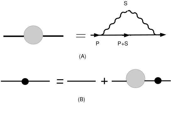
FIG. 1.: (A) HTL electron self energy with hard loop momenta; (B) Schwinger-Dyson equation for the HTL effective fermion propagator.

FIG. 2.: HTL effective vertex with hard loop momenta.

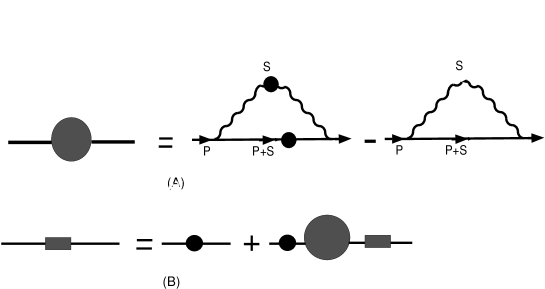
FIG. 3.: (A) Electron self energy in a second order effective theory; (B) Schwinger-Dyson equation for the fermion propagator in a second order effective theory.

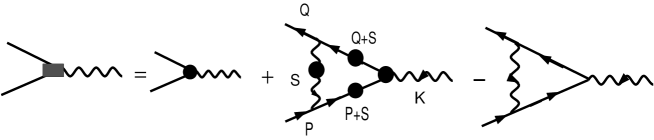
FIG. 4.: Effective vertex in a second order theory.

REFERENCES

• [1] E. Braaten and R.D. Pisarski, Nucl. Phys. B337, 569 (1990).
• [2] M.H. Thoma, in Quark-Gluon Plasma 2, edited by R. Hwa (World Scientific, Singapore, 1995), p.51.
• [3] J. Frenkel and J.C. Taylor, Nucl.Phys. B374, 156 (1992).
• [4] E. Braaten and R.D. Pisarski, Phys. Rev. D 45, R1827 (1992).
• [5] K. Chou, Z. Su, B. Hao, and L. Yu, Phys. Rep. 118, 1 (1985).
• [6] L.V. Keldysh, JETP 20, 1018 (1965).
• [7] M.E. Carrington, Hou Defu, and M.H.Thoma, hep-ph/9708363.
• [8] P.A. Henning, Phys. Rep. 253, 235 (1995).
• [9] M.E. Carrington and U. Heinz, Eur. Phys. J. C 1, 619 (1998).
Refer to caption