1 Introduction

1.1 Motivation

The Ising model is widely used for illustrating concepts in statistical mechanics and field theory. In 2-dimensions it is exactly solvable and provides the classic example of a theory which exhibits non-mean-field critical exponents. There are three representations of the model: That as a magnetic spin system, as a theory of random paths [2]-[5] and as a fermionic lattice field theory with Gaussian action (Grassmann representation) [6, 7, 9]. The connections between these are interesting, since they illustrate a deep relationship between dynamics and geometry. The random paths can be thought of as Euclidean world lines of the fermions and in turn as domain boundaries in the spin system.

Even more fascinating are the corresponding relationships in the 3-$D$ Ising model. The 3-$D$ model is not exactly solvable. However, it does share some of the geometrical features of the 2-$D$ model. Its partition function can be represented as a spin model, as a model of decorated random surfaces [13]-[16] and as a fermionic lattice model which is no longer Gaussian [6, 8, 10]. There is an intriguing suggestion [17, 18] that the continuum limit of the 3-$D$ Ising model could be some sort of non-critical string theory. The precise form of such a string theory is yet unknown.

Even the representation in terms of lattice surfaces (or loops) remains to be completely understood. In particular the calculus of surfaces (loops) is rather cumbersome to work with. Handling the symmetry and geometry factors in the loop and surface representations is a non-trivial problem. It would be desirable to have an exact algebraic representation of the geometrical objects. In this article we shall show that such an algebraic representation can be obtained from the hopping expansion (see e.g. [19]) of the Grassmann representation of the model. We obtain several new results which serve to demonstrate the power of this calculus.

The language of the hopping expansion allows for a simple algebraic formulation of the combinatorics of surfaces and loops. In particular all geometric factors are obtained as traces of ordered products of the hopping generators (= generators of shifts on the lattice). Also, counting problems which correspond to some symmetries of the geometric objects, such as iteration of loops (i.e. the loop runs through its links several times) can be tackled in a simple manner. As an application of the latter we shall give the corrected version of the loop expansion of the free energy in the 2-$D$ case. It differs from previous results by extra factors for iterated loops. Also the computation of the radius of convergence of loop- or surface expansion is a rather intractable problem if one has to work with the geometrical objects. For the 2-$D$ case we show that our calculus reduces this problem to the computation of the norm of the hopping matrix.

For the 3-$D$ case we derive a representation of the 3-$D$ Ising model as a product of 2-$D$ Ising models coupled to an auxiliary field. Based on this representation we give an elegant derivation of the geometric factor which eliminates overcounting of surfaces. Our approach also allows for a simple classification of surfaces to be summed over in the surface representation. We show that this classification can be reduced to a 2-dimensional problem: The surfaces can be characterized by the loops that emerge as intersections of the surfaces with the coordinate planes of the lattice. There is some freedom in the choice of admissible loops in these planes. Different choices lead to different classes of surfaces. For both 2- and 3-$D$ we derive an elegant formula for 2$n$-point functions in terms of loops and surfaces, respectively.

The paper is organized as follows: In Section 1.2 we review the representations of the Ising model in terms of loops (2-$D$) and surfaces (3-$D$) and introduce our conventions. Section 2 is dedicated to the 2-$D$ case. In 2.1 we set up the Grassmann representation and perform the hopping expansion. This is followed by Sub-section 2.2 where we show how to obtain the representation in terms of loops from the hopping expansion and show that the latter is an exact, algebraic representation of the loop calculus. The radius of convergence of the loop expansion of the free energy is shown to be determined by the critical temperature in 2.3.

Section 3 gives our results for the 3-$D$ case. In 3.1 we first decompose the quartic term in the Grassmann representation by introducing an auxiliary field and set up the hopping expansion. In 3.2 we extract the surface picture from the hopping expansion, derive the geometric factors and discuss the above mentioned classification of surfaces. In Sub-section 3.3 we derive the formula for the 2$n$-point functions in terms of surfaces (loops). The article closes with a discussion in Section 4.

1.2 Partition function, loops and surfaces

Since we will make extensive use of the representation of the partition function in terms of loops and surfaces we will review these representations here and introduce our conventions.

The Ising model in terms of spin variables has the partition function

$$Z\;=\;\sum_{\{s(x)=\pm 1\}}\exp\left(\beta\sum_{\langle x,y\rangle}s(x)s(y)\right)\;,$$ (1.1)

where $x$ runs over all sites of the $D$-dimensional lattice $\Lambda=$ZZ^D ($D=2,3)$ and $\langle x,y\rangle$ denotes nearest neighbors.

The 2-$D$ partition function has a representation in terms of closed loops [2]-[5],[16] on the dual lattice $\Lambda^{*}$ (for the square lattice $\Lambda\simeq\Lambda^{*}$). This representation is obtained by drawing closed loops $\gamma$ on the dual lattice around patches of negative spins on the original lattice. Each link in $\gamma$ crosses a link of the original lattice which has anti-aligned spins at its endpoints. By drawing loops around all such patches every anti-aligned link is taken into account. Each of these links has a Boltzmann weight exp$(-\beta)$, and since the total length $|\gamma|$ of all loops is equal the number of anti-aligned neighbors, this gives rise to the weight exp$(-\beta|\gamma|)$. If $V$ denotes the number of all sites, there remain $2V-|\gamma|$ links with aligned spins at the endpoints. They have Boltzmann weight exp$(+\beta)$ and one finds

$$Z\;=\;2\;t^{-2V}\sum_{\gamma\in{\cal L}_{ext}}(t^{2})^{|\gamma|}\;.$$ (1.2)

Here we introduced $t=$ exp$(-\beta)$. The factor 2 emerges, since every loop configuration corresponds to 2 spin configurations related by the ZZ₂ symmetry of the model. ${\cal L}_{ext}$ is defined to be the set of closed loops (not necessarily connected) which can be obtained by drawing lines on the dual lattice around patches of negative spins, so that a curve $\gamma$ in ${\cal L}_{ext}$ is given by a collection of links that have no boundary. This defines loops by their so-called extrinsic geometry. The series (1.2) will converge for small $t$, hence is a low temperature expansion (the convergence properties will be discussed in Section 2.3).

It is known that the partition function can also be written in terms of loops which have intrinsic geometry:

$$Z\;=\;2\;t^{-2V}\sum_{\gamma\in{\cal L}_{int}}(t^{2})^{|\gamma|}\;(-1)^{n(\gamma)}\;.$$ (1.3)

Here we introduced the number of self-intersections $n(\gamma)=0,1,2,\dots$ of a loop $\gamma$. We define ${\cal L}_{int}$ to be the set of all closed, not necessarily connected, loops $\gamma$ on the dual lattice with a fixed chosen orientation and with the restriction that each of the links of $\gamma$ is occupied only once. The loops may however intersect themselves or each other. Thus a loop $\gamma$ in ${\cal L}_{int}$ consists of a base point (or several base points when there are disconnected pieces) and a set of directions with the above restrictions. This is what we refer to as loops with intrinsic geometry.

A representation of the partition function in terms of loops with intrinsic geometry is a powerful tool, since it allows to exponentiate the sum over loops in (1.3). This gives an expression of the free energy in terms of loops. We will discuss the precise form of this representation later in detail. The density of the free energy is a well defined physical quantity also in the infinite volume limit, and its representation in terms of loops is a beautiful illustration of the interplay between dynamics and geometry.

There is a canonical mapping from ${\cal L}_{int}$ onto ${\cal L}_{ext}$, with the image of a loop $\gamma_{int}$ under this mapping given by the collection of links traced out by that loop $\gamma_{int}$. Obviously there exist many loops in ${\cal L}_{int}$ with distinct intrinsic geometries which get mapped to a single loop in ${\cal L}_{ext}$. However, the self-intersection factor $(-1)^{n(\gamma)}$ leads to a cancellation of this over-counting in the sum (1.3). This is illustrated in Fig. 1. Every pinch structure of a loop in ${\cal L}_{ext}$ (as depicted in Fig. 1, left-hand side) is the image of each of the three pieces of loops in ${\cal L}_{int}$ shown on the right-hand side of the figure.

Figure 1: Scheme for the cancellation of overcounting in the representation (1.3) using loops with intrinsic geometry. The left-most picture is the pinch-structure for the extrinsic geometry loop, and the other 3 pictures show the corresponding decomposition in the intrinsic geometry picture. The last one has an extra minus sign due to the intersection factor $(-1)^{n(\gamma)}$.

Note that larger classes of loops than ${\cal L}_{int}$ can be used to represent the Ising model. For example, the restriction that links are occupied only once in a loop can be relaxed to the restriction that the loops are non-back-tracking, i.e. they must not turn around at a site and run back on their last link. Again, the same self-intersection factor $(-1)^{n(\gamma)}$ gives rise to the necessary cancellations. However, for our presentation the above definition of ${\cal L}_{int}$ is most convenient.

It is straightforward to generalize (1.3) to the case of the variable bond Ising model, where the coupling $\beta_{\langle x,y\rangle}$ is allowed to vary over links $\langle x,y\rangle$. The generalization of (1.3) to the case of the variable bond model is given by

$$Z\;=\;2\prod_{\langle x,y\rangle}(t_{\langle x,y\rangle})^{-1}\sum_{\gamma\in{\cal L}_{int}}(-1)^{n(\gamma)}\prod_{\langle x,y\rangle\in\gamma^{*}}(t_{\langle x,y\rangle})^{2}\;.$$ (1.4)

Here we have generalized $t$ to $t_{\langle x,y\rangle}=$ exp$(-\beta_{\langle x,y\rangle})$ and $\gamma^{*}$ denotes the collection of links on the original lattice dual to the loop $\gamma$.

All of these representations can be generalized to the 3-$D$ case. The representation analogous to (1.2) is given by a sum over random surfaces with extrinsic geometry,

$$Z\;=\;2\;t^{-3V}\sum_{\sigma\in{\cal S}_{ext}}(t^{2})^{|\sigma|}\;.$$ (1.5)

Here ${\cal S}_{ext}$ denotes all closed, but not necessarily connected surfaces $\sigma$ made from plaquettes on the dual lattice which can be obtained by enclosing lumps of negative spins in the surface $\sigma$. Analogous to the 2-$D$ case the surface $\sigma$ in ${\cal S}_{ext}$ is a collection of plaquettes with zero boundary. We introduced the notation $|\sigma|$ for the area of the surface $\sigma$.

Also for the 3-$D$ case one is interested in a representation in terms of surfaces that allow for intrinsic geometry [6],[10],[13]-[16]. It is given by

$$Z\;=\;2\;t^{-3V}\sum_{\sigma\in{\cal S}_{int}}(t^{2})^{|\sigma|}\;(-1)^{L(\sigma)}\;.$$ (1.6)

Here $L(\gamma)$ denotes the number of links where the surface self-intersects. Again different choices for the set ${\cal S}_{int}$ of surfaces with intrinsic geometry are possible. We will be more explicit on the possible choices of ${\cal S}_{int}$ in Section 3, where we also give an elegant proof of formula (1.6).

2 The 2-D case

In this section we discuss the 2-dimensional case. This serves to outline the general strategy for the hopping expansion, to introduce some notation and we also obtain results that will be needed for the 3-$D$ case. Finally we give the correct result for the loop expansion of the free energy (exponentiation formula) which contains an additional factor for iterated loops which has previously been overlooked in the literature.

2.1 Grassmann representation and hopping expansion

The partition function in the form (1.2) can be written as an integral over Grassmann variables [6, 7, 9], which in two dimensions is given by

$$Z=\int\!\prod_{x\in\Lambda^{*}}d\eta_{-1}(x)d\eta_{+1}(x)d\eta_{-2}(x)d\eta_{+2}(x)\;e^{\beta[S_{L}(\eta)+S_{C}(\eta)+S_{M}(\eta)]}\;,$$ (2.1)

where the line-, corner- and monomer-terms of the action are given by

$$S_{L}(\eta)\!\!\! \!=\! \!\!t^{2}\sum_{x\in\Lambda^{*}}\!\left[\eta_{+1}(x)\eta_{-1}(x+\hat{1})+\eta_{+2}(x)\eta_{-2}(x+\hat{2})\right]\;,$$

$$S_{C}(\eta)\!\!\! \!=\! \!\!\!\!\sum_{x\in\Lambda^{*}}\!\left[\eta_{+1}(x)\eta_{-2}(x)\!+\!\eta_{+2}(x)\eta_{-1}(x)\!+\!\eta_{+2}(x)\eta_{+1}(x)\!+\!\eta_{-2}(x)\eta_{-1}(x)\right],$$

$$S_{M}(\eta)\!\!\! \!=\! \!\!\!\!\sum_{x\in\Lambda^{*}}\!\left[\eta_{-1}(x)\eta_{+1}(x)+\eta_{-2}(x)\eta_{+2}(x)\right]\;.$$ (2.2)

When the exponent in (2.1) is expanded, the non-vanishing contributions to the Grassmann integral exactly reproduce (without the overall factor $t^{-2V}$) the representation (1.2) of the partition function as a sum of loops with extrinsic geometry. The subscripts $L,C$ and $M$ refer to the elements: lines, corners and monomers of the loops as they are produced by the corresponding terms in the action. These building blocks give the extrinsic geometry loops in the following way: A line coming into a site has to have a partner going out. This property of having a partner is enforced by the integration rules for Grassmann variables. The outgoing line can continue in the direction of the incoming line, in this case the Grassmann integral is saturated by the monomer term. The outgoing line can also turn by $\pi/2$ in which case the Grassmann integral is made non-vanishing by the corner terms. The line can however not turn back since the square of a Grassmann variable vanishes. Finally there is the possibility that 4 lines are attached to a site and so saturate the Grassmann integral. This gives rise to the pinch structure already discussed above. Thus the loops produced by the expansion of (2.1) are closed (every incoming line has an outgoing partner) and non-back-tracking (square of the Grassmann variable vanishes). They are loops in extrinsic geometry since they simply occur as a set of links. Thus the expansion of (2.1) reproduces (1.2). For details concerning the ordering of the Grassmann variables see [7, 9].

For the following we need to write the action in a more compact and also anti-symmetrized form. We introduce the vector

$$\eta(x)\;=\;\Big{(}\eta_{+1}(x),\eta_{-1}(x),\eta_{+2}(x),\eta_{-2}(x)\Big{)}^{T}\;,$$ (2.3)

and the $4\times 4$ matrices $P_{\mu}(i,j)$ (the same matrices will be used in the 3-$D$ case where it is more convenient to denote them as $P_{\pm x}$ and $P_{\pm y})$

$$P_{+1}(i,j)\;\equiv\;P_{+x}(i,j)\;\equiv\;\delta_{i,1}\;\delta_{j,2} \;,\; P_{-1}(i,j)\;\equiv\;P_{-x}(i,j)\;\equiv\;-\delta_{i,2}\;\delta_{j,1}\;,$$

$$P_{+2}(i,j)\;\equiv\;P_{+y}(i,j)\;\equiv\;\delta_{i,3}\;\delta_{j,4} \;,\; P_{-2}(i,j)\;\equiv\;P_{-y}(i,j)\;\equiv\;-\delta_{i,4}\;\delta_{j,3}\;.$$

They obey $P_{\mu}^{T}=-P_{-\mu}$. We also define

$$M=\left(\begin{array}[]{cccc}0&-1&-1&+1\\ +1&0&-1&-1\\ +1&+1&0&-1\\ -1&+1&+1&0\end{array}\right)\;\;\;\;\;\mbox{with}\;\;\;\;\;M^{-1}=\left(\begin{array}[]{cccc}0&-1&+1&-1\\ +1&0&+1&+1\\ -1&-1&0&-1\\ +1&-1&+1&0\end{array}\right)\;.$$ (2.5)

We remark that $\det M=1$ and $M^{T}=-M$. With these definitions the action can be written as (the overall factor 1/2 comes from the anti-symmetrization)

$$S(\eta)\;=\;\frac{1}{2}\sum_{x,y\in\Lambda}\;\eta^{T}(x)\;K(x,y)\;\eta(y)\;\equiv\;\frac{1}{2}\eta^{T}K\eta\;,$$ (2.6)

where the kernel $K$ is given by

$$K(x,y)\;=\;M\delta(x,y)+t^{2}\!\sum_{\mu=\pm 1}^{\pm 2}P_{\mu}\;\delta(x+\hat{\mu},y)\;\equiv\;M\delta(x,y)+R(x,y)\;.$$ (2.7)

It is easy to see that $K$ is anti-symmetric. We remark that the representation (2.6), (2.7) is a natural way of writing the action for the Grassmann variables. It was already introduced in [11]. The partition function is given by a Pfaffian which, since $K$ is anti-symmetric, reduces to the root of a determinant

$$Z=\int d\eta\;e^{\frac{1}{2}\eta^{T}K\eta}=\;\mbox{Pf}\;K=\sqrt{\det K}\;=\;\sqrt{\det[M+R]}=\sqrt{\det[1+M^{-1}R]}.$$ (2.8)

Expanding the determinant one obtains

$$Z\;=\;\exp\left(-\frac{1}{2}\sum_{n=1}^{\infty}\frac{(-t^{2})^{n}}{n}\mbox{Tr}\;[H^{n}]\right),$$ (2.9)

where the hopping matrix $H$ is defined as $t^{2}H\equiv M^{-1}R$. In the last step we used the well known formula for the expansion of determinants of the form $\det[1-t^{2}H]$. This series converges for $t^{2}\parallel\!H\!\parallel_{\infty}<1$, and in Section 2.3 we will show that $t=t_{crit}\equiv\exp(-\beta_{crit})$ saturates this bound. The hopping matrix $H$ has the form

$$H(x,y)\;=\;\sum_{\mu=\pm 1}^{\pm 2}H_{\mu}\;\delta(x+\hat{\mu},y)\;\;\;\;\mbox{with}\;\;\;H_{\mu}\equiv M^{-1}P_{\mu}\;.$$ (2.10)

The trace of powers of $H$ is given by

$$\mbox{Tr}[H^{n}]\!\!\! = \!\!\sum_{x_{1},x_{2}\dots x_{n}}\sum_{\mu_{1},\mu_{2}\dots\mu_{n}}\!\!\delta(x_{1}+\hat{\mu}_{1},x_{2})\dots\delta(x_{n}+\hat{\mu}_{n},x_{1})\;\mbox{Tr}[H_{\mu_{1}}\dots H_{\mu_{n}}]$$

$$= \sum_{x_{1}}\sum_{\mu_{1},\mu_{2}\dots\mu_{n}}\delta(x_{1}+\hat{\mu}_{1}+\hat{\mu}_{2}+\dots\hat{\mu}_{n},x_{1})\;\mbox{Tr}\;[H_{\mu_{1}}H_{\mu_{2}}\dots H_{\mu_{n}}]\;.$$

Structures of this type are well known from the hopping expansion (see e.g. [19]) of the fermion determinant in lattice gauge theories with fermions. Due to the Kronecker delta the terms in the sum have support on closed loops. In the next section we will show that these loops have simple properties due to the algebra of the $H_{\mu}$’s and this will also lead to a straightforward computation of the trace $\mbox{Tr}\;[H_{\mu_{1}}H_{\mu_{2}}\dots H_{\mu_{n}}]$ for arbitrary closed loops $\gamma$.

2.2 Loop representation from the hopping expansion

From the remarks in the end of the last section it is clear that the loops supporting the contributions to (LABEL:htrace) are closed loops with a base point $x_{1}$ and described by the ordered set of directions $\{\mu_{1},\mu_{2},\dots\mu_{n}\}$, where each $\mu_{i}$ can have the values $\pm 1,\pm 2$. These loops are more general than the ones we included in ${\cal L}_{int}$. They are connected and are allowed to self-intersect, however in addition, they can occupy links several times or even iterate their whole path many times. Since closed loops have even length: Tr$[H^{2n+1}]=0$, and only even terms contribute in (2.9). Some examples of loops occuring in the hopping expansion are depicted in Fig. 2.

Figure 2: Some of the loops occuring in the hopping expansion. They differ from the loops in ${\cal L}_{int}$ since they can occupy links several times or iterate their whole path.

In order to compute the weights for the loops in (LABEL:htrace) the properties of the matrices $H_{\mu}=M^{-1}P_{\mu}$ have to be studied. The $H_{\mu}$-matrices will be encountered again in the 3-$D$ case where it will be convenient to denote them as $H_{\pm x}$ and $H_{\pm y}$. They are explicitly given by (compare [11])

$$H_{+1}\equiv H_{+x}=\left(\begin{array}[]{cccc}0&0&0&0\\ 0&+1&0&0\\ 0&-1&0&0\\ 0&+1&0&0\end{array}\right)\!\!\!\!\!\! \!H_{-1}\equiv H_{-x}=\left(\begin{array}[]{cccc}+1&0&0&0\\ 0&0&0&0\\ +1&0&0&0\\ +1&0&0&0\end{array}\right),$$ , (2.20)

$$H_{+2}\equiv H_{+y}=\left(\begin{array}[]{cccc}0&0&0&+1\\ 0&0&0&+1\\ 0&0&0&0\\ 0&0&0&+1\end{array}\right)\!\!\!\!\!\! \!H_{-2}\equiv H_{-y}=\left(\begin{array}[]{cccc}0&0&+1&0\\ 0&0&-1&0\\ 0&0&+1&0\\ 0&0&0&0\end{array}\right).$$ , (2.29)

We will now show that the algebra of these matrices restricts the set of loops occuring in the hopping expansion. The first observation is that $H_{\pm\mu}H_{\mp\mu}=0$, this property excludes back-tracking loops in (LABEL:htrace). Furthermore one can show that the trace of a product of $H_{\mu}$’s is invariant under reversing the orientation of the loop. This can be seen by using the definition $H_{\mu}=M^{-1}P_{\mu}$ and the transposition properties $P_{\mu}^{T}=-P_{-\mu}$ and $(M^{-1})^{T}=-M^{-1}$,

$$\mbox{Tr}\;[H_{-\mu_{2n}}H_{-\mu_{2n-1}}\dots H_{-\mu_{1}}] = \mbox{Tr}\;[M^{-1}P_{\mu_{2n}}^{T}\dots M^{-1}P_{\mu_{1}}^{T}]\;=$$

$$\mbox{Tr}\;[P_{\mu_{1}}M^{-1}\dots P_{\mu_{2n}}M^{-1}]^{T} = \mbox{Tr}\;[H_{\mu_{1}}H_{\mu_{2}}\dots H_{\mu_{2n}}]\;.$$

One can then fix an orientation for each loop in (LABEL:htrace) and write a factor 2 in front of the sum. This factor cancels the overall factor of 1/2 from the square root in (2.8).

Thus far we have shown that the paths which contribute in (LABEL:htrace) are closed, connected, non back-tracking loops, $\gamma$, with a chosen orientation. We finally prove that the trace over the product of $H_{\mu}$’s along a loop $\gamma$ yields the self-intersection factor

$$\mbox{Tr}\;\prod_{\mu\in\gamma}H_{\mu}\;=\;-(-1)^{n(\gamma)}\;.$$ (2.31)

As before $n(\gamma)$ denotes the number of self-intersections of the loop $\gamma$. The proof is decomposed into several steps. Using the explicit form (LABEL:hmatrices) of the $H_{\mu}$’s it is straightforward to show the following rules:

Basic loop:

$$\mbox{Tr}[H_{+1}H_{+2}H_{-1}H_{-2}]\;=\;-1\;.$$ (2.32)

Telescope rule:

$$H_{\mu}^{2}\;=\;H_{\mu}\;.$$ (2.33)

Kink rule:

$$H_{\mu}H_{\nu}H_{\mu}\;=\;H_{\mu}\;\;\;\mbox{for}\;\;\;\nu\neq-\mu\;.$$ (2.34)

Intersection rule:

$$(H_{+1})^{2}H_{+2}H_{-1}(H_{-2})^{2} = -H_{+1}H_{-2}\;,$$

$$(H_{+2})^{2}H_{+1}H_{-2}(H_{-1})^{2} = -H_{+2}H_{-1}\;.$$ (2.35)

The four rules have the obvious graphical interpretation depicted in Fig. 3.

Figure 3: Graphical representation of the rules for the reduction of $\mbox{Tr}\;[\prod_{\mu\in\gamma}H_{\mu}]$: basic loop (a), telescope rule (b), kink rule (c) and intersection rule (d) .

The result (2.32) is just formula (2.31) for the simplest loop, i.e. the one running around a single plaquette. Formula (2.33) allows one to stretch or shrink a loop without altering the trace (2.31). The kink rule (2.34) allows one to remove kinks in the path, and finally the intersection rule (2.35) allows one to remove sub-loops, giving rise to a factor of $-1$ for each self-intersection. Formula (2.35) gives the result (for both possible orientations) for the sub-loop depicted in Fig. 3 (d). The other 6 possibilities for (2.35) follow immediately from invariance of the formalism under rotations by $\pi/2$.

The above rules allow for a constructive reduction of the trace Tr$\prod_{\mu\in\gamma}H_{\mu}$ for an arbitrary closed, connected, non-back-tracking loop $\gamma$ as follows:

(1) Start with a sub-loop which has only one self-intersection point (an example for such a sub-loop is e.g. given in Fig. 4, second line). If the loop we started with has no self-intersection at all, proceed to (2), otherwise there exist at least two such sub-loops.

(2) Use telescope and kink rules to bring the sub-loop to the standard form as depicted in the left picture of Fig. 3 (d). Under these transformations the trace (2.31) remains invariant. In case the loop had no self-intersection to begin with, bring it to the standard form for loops without self-intersection as depicted in Fig. 3 (a), and (2.32) is the final result.

(3) Use the intersection rule to remove the sub-loop and collect an overall factor of $-1$. Repeat the steps (1) - (3) until finished.

We remark that if nested sub-loops coincide on some links, it is always possible to disentangle them using the telescope rule. Let’s elaborate a little bit more on the actual implementation of step (2): The idea is to replace products of $H_{\mu}$’s, corresponding to some sub-chain of links, by another product of $H_{\mu}$’s (obtained from the first one using kink and telescope rules), such that the new chain corresponds to a new piece of loop which is smoother, but still leaves the whole loop closed. The necessary condition for the new sub-chain to match the starting- and end-point of the old sub-chain is that the number of $+1$-moves minus the number of $-1$-moves as well as the number of $+2$-moves minus the number of $-2$-moves remains invariant (compare the example in Fig. 4 (a). In order to illustrate the steps involved we discuss two examples (see Fig. 4).

Figure 4: Examples for the reduction of loops: In step (a) telescope and kink rule were used to smoothen the dotted part of the loop (compare (2.36) for the corresponding algebraic expression). In step (b) we bring a sub-loop to canonical form, again using telescope and kink rule, and in step (c) the sub-loop is removed using the intersection rule giving an overall factor $-1$.

The first two pictures in Fig. 4 demonstrate how the telescope and kink rules are used to smoothen a contour (step (a) in the figure). The dotted part of the contour in the left figure is represented by the left-hand side of the following equation

$$H_{+1}H_{-2}H_{+1}H_{-2}\;=\;H_{+1}H_{-2}\;=\;(H_{+1})^{2}(H_{-2})^{2}\;.$$ (2.36)

Here we used the kink rule (2.34) to replace $H_{+1}H_{-2}H_{+1}$ by $H_{+1}$ and then expanded, using the telescope rule (2.33), to obtain the form on the right-hand side. This is once again a contour which matches starting- and end-points and corresponds to the second dotted contour in Fig. 4 (a). Thus step (a) in Fig. 4 is simply the replacement of the left-hand side of (2.36) inside some trace over $H_{\mu}$’s by its right-hand side. With combinations of telescope and kink rules all (sub-) loops can be transformed into squares, which can then be shrunk to loops around single plaquettes using the telescope rule. Under such a set of operations the trace (2.31) remains invariant. An example of such a transformation is depicted in step (b) of Fig. 4. Finally in step (c) of Fig. 4 the sub-loop is removed using the intersection rule (2.35) and an overall factor of $-1$ emerges. These steps can be applied iteratively to prove (2.31) for an arbitrary closed, connected, non-back-tracking loop $\gamma$.

On inserting (2.31) in (LABEL:htrace) and the result in (2.9) one finds

$$Z\;=\;\mbox{Pf}K\;=\;\exp\left(\sum_{n=1}^{\infty}\frac{(t^{2})^{2n}}{2n}\sum_{x}\sum_{\gamma\in L^{(2n)}_{x}}(-1)^{n(\gamma)}\right)\;.$$ (2.37)

Here $L_{x}^{(2n)}$ denotes the set of closed, connected, non-back-tracking loops of length $2n$ based at $x$ with a chosen orientation. Recall that (LABEL:htrace) is non-vanishing only for even $n$ and thus the alternating sign of (2.9) disappears. The overall factor of 1/2 in (2.9) is gone since we chose only one of the two possible orientations of a loop, and the overall minus sign in (2.9) is cancelled by the overall sign in (2.31).

It is possible to simplify the exponential in (2.37) even further: To do that we discuss (in order of increasing complexity) loops with singly occupied links, iterated loops where the whole set of links is run through several times and finally loops where only some links are occupied several times. To start take some loop $\gamma$ in $L_{x}^{(2n)}$ where each link in the loop is occupied only once. For the contour corresponding to this loop $\gamma$ there are all together $2n$ inequivalent choices of a base point. Each of these points can serve as the base point for a different loop giving rise to the same contribution to (2.37) as $\gamma$. As such, one can choose a single representative of this class of loops and remove the factor of $1/2n$ in (2.37). Now consider a loop which runs through its contour twice, i.e. each link occurs exactly twice (an example of such a loop is given in Fig. 2 (c)). For such an iterated loop we have only $2n/2$ possible choices of inequivalent base points. In general for a loop $\gamma$ that is iterated $I(\gamma)$-times there are $2n/I(\gamma)$ inequivalent choices for the base point. As for the non-iterated loops, one can choose a single representative and remove the factor of $1/2n$ in (2.37), however, the factor of $1/I(\gamma)$ remains. Finally we remark that for loops where only a sub-loop is iterated no such factor can occur, since the set of directions $\mu_{1},\mu_{2}\dots\mu_{2n}$ is different (cyclicly permuted) for some starting point $x$, and the same point visited by the loop after running through a sub-loop. The partition function thus reads:

$$Z\;=\;\mbox{Pf}K\;=\;\exp\left(\sum_{\gamma\in{\cal L}^{con}_{exp}}(t^{2})^{|\gamma|}\;(-1)^{n(\gamma)}\;\frac{1}{I(\gamma)}\right)\;,$$ (2.38)

where ${\cal L}_{exp}^{con}$ denotes the set of all closed, connected, non-back-tracking loops (without base point) and $I(\gamma)$ is the number of iterations of the loop $\gamma$.

We stress that this result differs from previous formulas for the exponentiation of (1.3) by the factor $1/I(\gamma)$ for iterated loops. This factor is, however, essential for the correct cancellation of loops that have no counterpart in ${\cal L}_{ext}$. This can be seen by the following simple example: Consider the basic loop of length 4 which runs around a plaquette. When the exponent in (2.38) is expanded, this loop will, in the quadratic term of the expansion, give rise to the plaquette which is occupied by two such loops running around this single plaquette (see the left-hand side of Fig. 5). It has the factor $t^{16}/2$, where the factor 1/2 comes from the expansion of the exponential function. This loop has no counterpart in ${\cal L}_{ext}$ and thus has to be cancelled by some other loop. It is clear that the only loop which can cancel this loop is the one depicted on the right-hand side of Fig. 5. It appears in the linear term of the expansion of the exponential function and comes with the factor $-t^{16}/2$ and thus exactly cancels the first loop. The overall minus sign is due to the self-intersection and the factor 1/2 comes from the term $I(\gamma)^{-1}$. Hence this factor is essential for the cancellation of unphysical loops.

Figure 5: Example for the cancellation of an iterated loop. The figure on the left-hand side shows the contribution of the basic loop around a single plaquette in the quadratic term of the expansion of the exponential in (2.38). Here the factor 1/2 comes from the power series expansion of the exponential function. The picture on the right-hand side shows the contribution of the iterated loop, which appears in the linear term of the expansion. Here the factor 1/2 comes from the iteration term $1/I(\gamma)$. The self intersection term produces the minus sign which ensures the cancellation of the two contributions.

With the derivation of (2.38) we have established that the hopping expansion (2.9) of the Grassmann formulation gives an exact algebraic representation of the loop expansion.

It is straightforward to generalize (2.38) to the case of the variable bond Ising model by running through the derivation once more but allowing for varying Boltzmann factors $t_{\langle x,y\rangle}=$ exp$(-\beta_{\langle x,y\rangle})$. The result is (neglecting the overall factor $2\prod(t_{\langle x,y\rangle})^{-1}$):

$$Z=\exp\left(\sum_{\gamma\in{\cal L}^{con}_{exp}}\frac{(-1)^{n(\gamma)}}{I(\gamma)}\;\prod_{\langle x,y\rangle\in\gamma^{*}}(t_{\langle x,y\rangle})^{2}\right)\;.$$ (2.39)

We remark that when a loop $\gamma$ occupies some links several times, its dual $\gamma^{*}$ has multiply occupied links. Thus in the last equation the product includes a link-factor whenever the link is intersected by the loop. In particular for iterated loops each link factor $(t_{\langle x,y\rangle})^{2}$ occurs $I(\gamma)$-times.

2.3 Radius of convergence and critical temperature

The formula (2.38) is a physically interesting result, since the exponent is proportional to the loop expansion of the free energy density $f$

$$f\;=\;-\frac{1}{\beta}\lim_{V\rightarrow\infty}\frac{1}{V}\sum_{\gamma\in{\cal L}^{con}_{exp}}(t^{2})^{|\gamma|}\;(-1)^{n(\gamma)}\;\frac{1}{I(\gamma)}\;.$$ (2.40)

The sum (2.40) will converge for sufficiently small $t$, and the radius of convergence corresponds to the critical temperature. However, computing the radius of convergence of the loop expansion in the form (2.40) is a rather intractable problem. It is very convenient to make use of the form (2.9) of the expansion, where it is clear that the expansion converges for

$$t^{2}\parallel\!\!H\!\!\parallel_{\infty}\;<\;1\;.$$ (2.41)

The norm $\parallel\!H\!\parallel_{\infty}$ is defined as sup${}_{\parallel t\parallel=1}\sqrt{(t,H^{\dagger}Ht)}$ where $t$ is some test-function and $\parallel\!t\!\parallel=\sqrt{(t,t)}$, and the inner product is defined to be the $l^{2}$ product obtained by summing over all lattice and spinor indices. It is straightforward to compute

$$H^{\dagger}H\!=\!\left(\!\!\!\begin{array}[]{cccc}3\delta(x,y)&0&\!\!\!\!\!2\delta(x\!+\!\hat{1}\!-\!\hat{2},y)&2\delta(x\!+\!\hat{1}\!+\!\hat{2},y)\\ 0&3\delta(x,y)&\!\!\!\!\!-2\delta(x\!-\!\hat{1}\!-\!\hat{2},y)&2\delta(x\!-\!\hat{1}\!+\!\hat{2},y)\\ 2\delta(x\!-\!\hat{1}\!+\!\hat{2},y)&-2\delta(x\!+\!\hat{1}\!+\!\hat{2},y)&\!\!\!\!\!3\delta(x,y)&0\\ 2\delta(x\!-\!\hat{1}\!-\!\hat{2},y)&2\delta(x\!+\!\hat{1}\!-\!\hat{2},y)&\!\!\!\!\!0&3\delta(x,y)\end{array}\!\!\!\right)\!.$$

The lattice indices of this matrix can be diagonalized using Fourier transformation, giving

$$F^{\dagger}H^{\dagger}HF(p,q)=\delta(p,q)\!\left(\!\!\!\begin{array}[]{cccc}3&\!0&\!\!\!\!2e^{-ip_{1}+ip_{2}}&2e^{-ip_{1}-ip_{2}}\\ 0&\!3&\!\!\!\!-2e^{+ip_{1}+ip_{2}}&2e^{+ip_{1}-ip_{2}}\\ 2e^{+ip_{1}-ip_{2}}&\!-2e^{-ip_{1}-ip_{2}}&\!\!\!\!3&0\\ 2e^{+ip_{1}+ip_{2}}&\!2e^{-ip_{1}+ip_{2}}&\!\!\!\!0&3\end{array}\!\!\!\right)\!,$$

where the transformation matrix $F$ is given by $F(y,q)=\exp(-iyq)/2\pi$. The eigenvalues $\lambda$ for the remaining $4\times 4$ problem can be easily computed giving (each $\lambda$ is two-fold degenerate)

$$\lambda_{\pm}\;=\;3\pm 2\sqrt{2}\;.$$ (2.42)

The norm $\parallel\!H\!\parallel_{\infty}$ is then given by the square root of the larger eigenvalue. From (2.41) and (2.42) we obtain for the critical $t_{c}=e^{-\beta_{c}}$:

$$1\;=\;(t_{c})^{2}\parallel\!H\!\parallel\;=\;e^{-2\beta_{c}}\sqrt{3+2\sqrt{2}}\;\;\;\Longrightarrow\;\;\;\beta_{c}\;=\;\frac{1}{2}\ln(1+\sqrt{2})\;.$$ (2.43)

This is the well known result for the critical inverse temperature. We thus have achieved an elegant proof that the radius of convergence of the loop expansion (2.40) for the free energy is determined by the critical temperature. Computing the radius of convergence of (2.40) without the Grassmann representation is a rather intractable problem.

3 The 3-D case

We now discuss the 3-$D$ case. We will see that the 3-$D$ model factorizes into products of 2-$D$ models coupled to an auxiliary field and many of the concepts developed in the previous section will become very useful.

3.1 Grassmann representation and hopping expansion

Also for the 3-$D$ case there exists a Grassmann integral for the representation of the partition function in terms of surfaces with extrinsic geometry [6, 8, 10]. Here we use a notation different from the original work, which is however more convenient for our expansion.

Each link of the dual lattice carries 4 Grassmann variables denoted by $\eta_{\pm\nu}(x,\mu)$ as depicted in Fig. 6. Here $x$ and $\mu$ denote the link the variable lives on, and $\pm\nu$ distinguishes the 4 different variables on each link.

Figure 6: Labeling of the Grassmann variables $\eta_{\pm\nu}(x,\mu)$ associated with the links of the dual lattice.

The action for the Grassmann variables is again a sum of three terms $S=S_{P}+S_{E}+S_{M}$ producing the elements of the surfaces: plaquettes, edges and monomers. The terms are given by

$$S_{P}[\eta] = t^{2}\sum_{x}\sum_{\stackrel{{\scriptstyle\scriptstyle\mu,\nu=1}}{{\mu<\nu}}}^{3}\eta_{+\mu}(x,\nu)\eta_{-\mu}(x+\hat{\mu},\nu)\;\eta_{+\nu}(x,\mu)\eta_{-\nu}(x+\hat{\nu},\mu)\;,$$

$$S_{E}[\eta] = \sum_{x}\sum_{\mu=1}^{3}\sum_{\stackrel{{\scriptstyle\scriptstyle\nu,\rho\neq\mu}}{{\nu<\rho}}}\Big{[}\eta_{+\nu}(x,\mu)\eta_{-\rho}(x,\mu)+\eta_{+\rho}(x,\mu)\eta_{+\nu}(x,\mu)$$

$$+ \eta_{+\rho}(x,\mu)\eta_{-\nu}(x,\mu)+\eta_{-\rho}(x,\mu)\eta_{-\nu}(x,\mu)\Big{]}\;,$$

$$S_{M}[\eta] = \sum_{x}\sum_{\mu=1}^{3}\sum_{\stackrel{{\scriptstyle\scriptstyle\nu,\rho\neq\mu}}{{\nu<\rho}}}\Big{[}\eta_{-\nu}(x,\mu)\eta_{+\nu}(x,\mu)+\eta_{-\rho}(x,\mu)\eta_{+\rho}(x,\mu)\Big{]}\;.$$ (3.1)

The Grassmann representation of the 3-$D$ Ising model [6, 8, 10] is a straightforward generalization of the 2-$D$ case. Again the exponential of (3.1) has to be expanded, and the Grassmann integral reproduces the terms corresponding to the representation of the partition function in terms of surfaces with extrinsic geometry. Similar to the 2-$D$ case plaquettes, produced by $S_{P}$, that are incoming to a link must have an outgoing partner to saturate the Grassmann integral. Possible choices for the direction of the outgoing plaquette are either the same direction as the incoming plaquette (monomer terms) or rotated by $\pi/2$ (edge terms). The outgoing plaquette can however not fold back on the incoming one due to the fact that the square of a Grassmann variable vanishes. Also 4 plaquettes attached to a link can saturate the Grassmann integral, producing the pinch structure of the surfaces. The resulting terms of the Grassmann integral thus correspond to the closed surfaces in ${\cal S}_{ext}$. For details concerning the ordering of the Grassmann variables see [6, 8, 10].

The quartic interaction, from $S_{P}[\eta]$, can be decomposed into a Yukawa-like term with a tensor field by using the following identity for Grassmann variables $\eta_{1},\eta_{2},\eta_{3},\eta_{4}$

$$\exp\left(t^{2}\eta_{1}\eta_{2}\eta_{3}\eta_{4}\right)=\frac{1}{2}\sum_{A=\pm 1}\exp\Big{(}t~{}A~{}[\eta_{1}\eta_{2}+\eta_{3}\eta_{4}]\Big{)}\;.$$ (3.2)

Thus, $S_{P}[\eta]$ can be replaced by

$$S_{P}[\eta,A]=t\sum_{x}\sum_{\stackrel{{\scriptstyle\scriptstyle\mu,\nu=1}}{{\mu<\nu}}}^{3}A_{\mu\nu}(x)\Big{[}\eta_{+\mu}(x,\nu)\eta_{-\mu}(x+\hat{\mu},\nu)+\eta_{+\nu}(x,\mu)\eta_{-\nu}(x+\hat{\nu},\mu)\Big{]},$$ (3.3)

and the partition function now contains a sum over auxiliary fields $A_{\mu\nu}(x)$ associated with the plaquettes $(x;\mu,\nu)$ of the dual lattice,

$$Z\;=\;\left(\frac{1}{2}\right)^{3V}\sum_{\{A_{\mu\nu}(x)=\pm 1\}}\int d\eta\;e^{S_{P}[\eta,A]+S_{E}[\eta]+S_{M}[\eta]}\;.$$ (3.4)

The introduction of the auxiliary fields transformed the action for the Grassmann variables to a quadratic form, and the hopping expansion methods can be applied. As in the 2-$D$ case, the next step is to introduce the vectors $\psi(x)$ containing all 12 variables living on the 3 links associated with the site $x$ of the dual lattice

$$\psi(x) = \Big{(}\eta_{+2}(x,1),\eta_{-2}(x,1),\eta_{+3}(x,1),\eta_{-3}(x,1),\eta_{+1}(x,2),\eta_{-1}(x,2),$$

$$\eta_{+3}(x,2),\eta_{-3}(x,2),\eta_{+1}(x,3),\eta_{-1}(x,3),\eta_{+2}(x,3),\eta_{-2}(x,3)\Big{)}^{T}\;.$$

With this ordering of the variables, the edge and monomer terms of the action can be written as a quadratic form $S_{E}+S_{M}=1/2\psi^{T}\widetilde{M}\;\psi$, which is a simple generalization of the expression already used in the 2-$D$ case. The kernel $\widetilde{M}$ for the corresponding terms is block-diagonal, with the blocks given by the matrix $M$ from the 2-$D$ formulation (2.5),

$$\widetilde{M}\;\equiv\;\mbox{diag}\;\Big{(}1,1,1\Big{)}\otimes M\;.$$ (3.5)

$\widetilde{M}$ inherits the following properties from $M$: det $\widetilde{M}=1,\widetilde{M}^{T}=-\widetilde{M}$ and $\widetilde{M}^{-1}=$ diag$(1,1,1)\otimes M^{-1}$ with $M^{-1}$ given in (2.5). Also, the terms containing the auxiliary fields have a simple form if one makes use of the matrices $P_{\pm x},P_{\pm y}$ already defined in (LABEL:pmatrix),

$$S_{P}\;=\;\frac{t}{2}\sum_{x}\sum_{\mu=\pm 1}^{\pm 3}\psi(x)^{T}B_{\mu}(x)\psi(x+\hat{\mu})\;,$$ (3.6)

where the fields $B_{\mu}$ are composed from the auxiliary fields $A_{\mu\nu}(x)$ as follows:

$$B_{+1}(x) = A_{12}(x)\;\mbox{diag}(0,1,0)\otimes P_{+x}+A_{13}(x)\;\mbox{diag}(0,0,1)\otimes P_{+x}\;,$$

$$B_{+2}(x) = A_{12}(x)\;\mbox{diag}(1,0,0)\otimes P_{+x}+A_{23}(x)\;\mbox{diag}(0,0,1)\otimes P_{+y}\;,$$

$$B_{+3}(x) = A_{13}(x)\;\mbox{diag}(1,0,0)\otimes P_{+y}+A_{23}(x)\;\mbox{diag}(0,1,0)\otimes P_{+y}\;,$$

$$B_{-\mu}(x) = -B_{+\mu}(x-\hat{\mu})^{T}\;\;\;\;,\;\;\mu=1,2,3\;.$$ (3.7)

Using these definitions, the action takes the simple form,

$$S\;=\;\frac{1}{2}\sum_{x,y}\psi(x)^{T}K(x,y)\;\psi(y)\;,$$ (3.8)

where,

$$K(x,y)\;=\;\widetilde{M}\;\delta(x,y)\;+\;t\sum_{\mu=\pm 1}^{\pm 3}B_{\mu}(x)\;\delta(x+\hat{\mu},y)\;.$$ (3.9)

The kernel $K$ is obviously anti-symmetric. With this form for the action, the partition function can be partially evaluated,

$$Z = 2^{-3V}\!\!\sum_{\{A_{\mu\nu}(x)\}}\int d\psi\;e^{\frac{1}{2}\psi^{T}K\psi}=2^{-3V}\!\!\sum_{\{A_{\mu\nu}(x)\}}\mbox{Pf}K$$ (3.10)

$$= 2^{-3V}\!\!\sum_{\{A_{\mu\nu}(x)\}}\sqrt{\mbox{det}K}=2^{-3V}\!\!\sum_{\{A_{\mu\nu}(x)\}}\sqrt{\mbox{det}\widetilde{M}\;\mbox{det}[1+tH]}$$

As in the 2-$D$ case the determinant can be expanded (use det$\widetilde{M}=1$) to give the expansion for the partition function,

$$Z\;=\;2^{-3V}\!\!\sum_{\{A_{\mu\nu}(x)\}}\exp\left(-\frac{1}{2}\sum_{n=1}^{\infty}\frac{(-t)^{n}}{n}\mbox{Tr}[H^{n}]\right)\;,$$ (3.11)

where the hopping matrix $H$ takes the form

$$H(x,y)\;=\;\sum_{\mu=\pm 1}^{\pm 3}C_{\mu}(x)\;\delta(x+\hat{\mu},y)\;.$$ (3.12)

The fields $C_{\mu}(x)$ are obtained from $B_{\mu}(x)$ by multiplication with $\widetilde{M}^{-1}$ from the left. Making use of the block-diagonal form of $\widetilde{M}$ we find their explicit expression

$$C_{+1}(x) = A_{12}(x)\;\mbox{diag}(0,1,0)\otimes H_{+x}+A_{13}(x)\;\mbox{diag}(0,0,1)\otimes H_{+x},$$

$$C_{-1}(x)\! = \!A_{12}(x-\hat{1})\;\mbox{diag}(0,1,0)\otimes H_{-x}+A_{13}(x-\hat{1})\;\mbox{diag}(0,0,1)\otimes H_{-x},$$

$$C_{+2}(x)\! = \!A_{12}(x)\;\mbox{diag}(1,0,0)\otimes H_{+x}+A_{23}(x)\;\mbox{diag}(0,0,1)\otimes H_{+y},$$

$$C_{-2}(x)\! = \!A_{12}(x-\hat{2})\;\mbox{diag}(1,0,0)\otimes H_{-x}+A_{23}(x-\hat{2})\;\mbox{diag}(0,0,1)\otimes H_{-y},$$

$$C_{+3}(x)\! = \!A_{13}(x)\;\mbox{diag}(1,0,0)\otimes H_{+y}+A_{23}(x)\;\mbox{diag}(0,1,0)\otimes H_{+y},$$

$$C_{-3}(x)\! = \!A_{13}(x-\hat{3})\;\mbox{diag}(1,0,0)\otimes H_{-y}+A_{23}(x-\hat{3})\;\mbox{diag}(0,1,0)\otimes H_{-y},$$

The hopping generators $H_{\pm x},H_{\pm y}$ were already used in the 2-$D$ case (LABEL:hmatrices). To compute the partition function we once again must study the traces of powers of the hopping matrix,

$$\mbox{Tr}[H^{n}]\!\! = \!\!\sum_{x}\sum_{\mu_{1},\dots\mu_{n}}\delta(x+\hat{\mu}_{1}+\dots+\hat{\mu}_{n},x)$$ (3.14)

$$\!\!\mbox{Tr}[C_{\mu_{1}}(x)C_{\mu_{2}}(x+\hat{\mu}_{1})\dots C_{\mu_{n}}(x+\hat{\mu}_{1}+\dots+\hat{\mu}_{n-1})].$$

The result is similar to the 2-$D$ case but the remaining traces now also depend on $x$. Again it can be seen immediately from the Kronecker delta, that the terms in the sum have support on connected, closed loops with base point $x$. The fact that closed loops have even length forces Tr$[H^{n}]$ to vanish for odd $n$.

We remark that since the partition function (3.11) is now a sum over auxiliary fields a simple computation of the radius of convergence of the expansion is not available. This also prevents a simple exponentiation of the terms in the statistical sum to obtain the free energy. For an alternative approach, using different geometric factors see [15].

3.2 Surfaces

In this section we will show that the expansion (3.10), (3.11), (3.14) gives rise to an interpretation in terms of surfaces with intrinsic geometry (see also [6], [10], [13]-[16]). There is however an intermediate step, which we discuss first, where the terms in (3.14) are interpreted as loops corresponding to ribbons of plaquettes.

It was already mentioned that the loops supporting the contributions to (3.14) have to be closed and connected. Using essentially the same arguments as in the 2-$D$ case one can show that the trace over the fields $C_{\mu}(x)$ remains invariant under reversing the orientation of the loop. Thus, as in the 2-$D$ case, one can fix an orientation for each loop and write a factor 2 in front of the sum in (3.14), which will later cancel the factor of 1/2 from the square root in (3.11).

It is crucial to observe, that the special form (LABEL:cfields) of the matrix valued fields $C_{\mu}(x)$ reduces the contributions to (3.14) to effectively 2-dimensional objects. In particular the matrices diag$(1,0,0)$, diag$(0,1,0)$, diag$(0,0,1)$ in (LABEL:cfields) form a complete set of projectors, corresponding to the three coordinate planes of the dual lattice. This has two important implications:

Firstly we note, that the loops in (3.14) are non-back-tracking. This is a consequence of $H_{\pm\mu}H_{\mp\mu}=0$ (compare the discussion for the 2-$D$ case) and the fact that the mentioned projectors do not allow for cross-terms in $C_{\pm\mu}(x)C_{\mp\mu}(x\pm\hat{\mu})$ (each $C_{\mu}(x)$ is a sum of two terms).

Secondly, the projectors imply that the choice of just two of the matrices $C_{\mu}(x)$ in the trace Tr$[C_{\mu_{1}}(x)\dots C_{\mu_{2n}}(x+\mu_{1}+\dots+\mu_{2n-1})]$ already fixes a coordinate plane for all the terms in this trace. Assume, for example, that the first factor in the trace is one of $C_{\pm 1}(x)$ and any other factor is one of $C_{\pm 2}(x)$, then from the explicit representation (LABEL:cfields) it is clear that only the terms containing the projector diag$(0,0,1)$ can contribute. One is confined to the 1-2 plane, since only the $C_{\pm 1}(x)$ and $C_{\pm 2}(x)$ contain this projector. The formula for all terms in this plane (i.e. all terms associated with the projector diag$(0,0,1)$) can be read of from (3.14) and (LABEL:cfields) and is given by

$$2\sum_{x}\sum_{\gamma\in L^{(2n)}_{x,12}}\mbox{Tr}\Big{[}\prod_{\mu\in\gamma}H_{\mu}\Big{]}\;\prod_{(y,\nu)\in\gamma}A_{\nu 3}(y)\;.$$ (3.15)

To abbreviate the notation we defined $A_{-\nu 3}(y)\equiv A_{\nu 3}(y-\hat{\nu})$ for $\nu=1,2$. The set $L^{(2n)}_{x,12}$ is defined to be the set of all closed, non-back-tracking loops with a chosen orientation and length $2n$ in the 1-2 plane, with base point $x$. In the product under the trace the indices $\mu$ of $H_{\mu}$ can have the values $\pm x,\pm y$ (corresponding to $\pm 1$ and $\pm 2$ directions on the dual lattice). The trace was already computed in the 2-$D$ case and the result is $-(-1)^{n(\gamma)}$. The product over the auxiliary field picks up all the terms $A_{\nu 3}(x)$ along the loop $\gamma$.

Actually the geometrical objects that appear in the above sum should be thought of as ribbons of plaquettes. These ribbons are defined to be the set of plaquettes spanned by the links of $\gamma$ together with the unit vector in $\hat{3}$-direction. In the above expression (3.15) one can interpret the ribbons as being dressed with the auxiliary fields $A_{\mu 3}(x)$ defined on the plaquettes of the ribbon. For the other coordinate planes the ribbons are constructed likewise. The concept of ribbons is illustrated in Fig. 7.

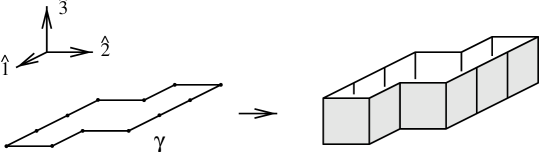
Figure 7: Example for a loop $\gamma$ in the 1-2-plane and the ribbon spanned by the links of $\gamma$ together with the unit vector in 3-direction.

The contributions to (3.14) in the other two coordinate planes have the same structure as (3.15), giving the final result

$$\mbox{Tr}[H^{2n}] = \!\!-2\sum_{x}\Big{(}\sum_{\gamma\in L^{(2n)}_{x,12}}(-1)^{n(\gamma)}\prod_{(y,\nu)\in\gamma}A_{\nu 3}(y)$$

$$+ \!\!\!\!\sum_{\gamma\in L^{(2n)}_{x,13}}(-1)^{n(\gamma)}\prod_{(y,\nu)\in\gamma}A_{\nu 2}(y)+\sum_{\gamma\in L^{(2n)}_{x,23}}(-1)^{n(\gamma)}\prod_{(y,\nu)\in\gamma}A_{\nu 1}(y)\Big{)}.$$

To shorten our notation we identified $A_{\mu\nu}(x)\equiv A_{\nu\mu}(x)$ and introduced $A_{-\mu\nu}(x)\equiv A_{\mu\nu}(x-\hat{\mu})$ (both definitions for $\mu,\nu=1,2,3;\mu\neq\nu$).

Inserting the result for the trace Tr$[H^{2n}]$ into the expansion (3.11) and this into the expression (3.10) for the partition function one ends up with

$$Z=2^{-3V}\sum_{\{A_{\mu\nu}(x)=\pm 1\}}\! \!\prod_{x_{3}}\exp\left(\sum_{\gamma\in{\cal L}^{con}_{exp}(12,x_{3})}\frac{(-1)^{n(\gamma)}}{I(\gamma)}\;t^{|\gamma|}\;\prod_{(y,\nu)\in\gamma}A_{\nu 3}(y)\right)$$

$$\!\prod_{x_{2}}\exp\left(\sum_{\gamma\in{\cal L}^{con}_{exp}(13,x_{2})}\frac{(-1)^{n(\gamma)}}{I(\gamma)}\;t^{|\gamma|}\;\prod_{(y,\nu)\in\gamma}A_{\nu 2}(y)\right)$$

$$\!\prod_{x_{1}}\exp\left(\sum_{\gamma\in{\cal L}^{con}_{exp}(23,x_{1})}\frac{(-1)^{n(\gamma)}}{I(\gamma)}\;t^{|\gamma|}\;\prod_{(y,\nu)\in\gamma}A_{\nu 1}(y)\right)\;.$$

This formula is a representation of the 3-$D$ Ising model as a product of 2-$D$ Ising models in their loop representation coupled to an external field. We introduced ${\cal L}^{con}_{exp}(12,x_{3})$ to be the set of loops ${\cal L}^{con}_{exp}$ already discussed in the 2-$D$ case, but living in particular in the 1-2 plane of the 3-$D$ lattice with 3-coordinate $x_{3}$. The sets ${\cal L}^{con}_{exp}(13,x_{2})$ and ${\cal L}^{con}_{exp}(23,x_{1})$ are defined likewise. By comparing (LABEL:3za) with the 2-$D$ expression (2.39) one finds that the 3-$D$ partition function is a product of 2-$D$ partition functions with locally varying Boltzmann factors $tA_{\mu\nu}(x)$. Making use of the fact that the representations (2.39) and (1.4) are equal (drop the overall factor in (1.4)) we obtain

$$Z=2^{-3V}\sum_{\{A_{\mu\nu}(x)=\pm 1\}}\! \!\!\!\prod_{x_{3}}\left(\sum_{\gamma\in{\cal L}_{int}(12,x_{3})}\!\!\!(-1)^{n(\gamma)}\;t^{|\gamma|}\;\prod_{(y,\nu)\in\gamma}A_{\nu 3}(y)\right)$$

$$\!\!\!\prod_{x_{2}}\left(\sum_{\gamma\in{\cal L}_{int}(13,x_{2})}\!\!\!(-1)^{n(\gamma)}\;t^{|\gamma|}\;\prod_{(y,\nu)\in\gamma}A_{\nu 2}(y)\right)$$

$$\!\!\!\prod_{x_{1}}\left(\sum_{\gamma\in{\cal L}_{int}(23,x_{1})}\!\!\!(-1)^{n(\gamma)}\;t^{|\gamma|}\;\prod_{(y,\nu)\in\gamma}A_{\nu 1}(y)\right)$$

$$=\prod_{x_{1},x_{2},x_{3}}\sum_{\stackrel{{\scriptstyle\scriptstyle\gamma_{12}\in{\cal L}_{int}(12,x_{3})}}{{\stackrel{{\scriptstyle\scriptstyle\gamma_{13}\in{\cal L}_{int}(13,x_{2})}}{{\gamma_{23}\in{\cal L}_{int}(23,x_{1})}}}}}\!\!\! t^{|\gamma_{12}|+|\gamma_{13}|+|\gamma_{23}|}\;(-1)^{n(\gamma_{12})+n(\gamma_{13})+n(\gamma_{23})}$$

$$2^{-3V}\!\!\!\!\!\!\sum_{\{A_{\mu\nu}(x)=\pm 1\}}\!\!\!\!\!\!\prod_{\;\;\;\;(y_{12},\nu_{12})\in\gamma_{12}}\!\!\!\!\!\!A_{\nu_{12}3}\!\!\!\!\! \!\!\!\!\!\!(y_{12})\!\!\!\!\!\prod_{\;\;\;\;(y_{13},\nu_{13})\in\gamma_{13}}\!\!\!\!\!A_{\nu_{13}2}(y_{13})\!\!\!\prod_{\;\;\;\;(y_{23},\nu_{23})\in\gamma_{23}}\!\!\!\!\!A_{\nu_{23}1}(y_{13}).$$

${\cal L}_{int}(12,x_{3})$ is the set of loops ${\cal L}_{int}$ defined in the 2-$D$ case, but living in the 1-2 coordinate plane with 3-coordinate $x_{3}$. ${\cal L}_{int}(13,x_{2})$ and ${\cal L}_{int}(23,x_{1})$ are defined likewise. The representation (LABEL:surf1) has an interesting interpretation in terms of surfaces. The last term in (LABEL:surf1), i.e. the sum over products of $A_{\mu\nu}(x)$, is non-vanishing only if each $A_{\mu\nu}(x)$ occurs an even number of times otherwise the sum will cancel terms which differ only by a minus sign. All non-vanishing contributions to the sum can be given a geometrical interpretation. This is achieved by associating a ribbon to every loop (as described earlier), and then dressing the ribbons with the auxiliary fields $A_{\mu\nu}(x)$ defined on the plaquettes of that ribbon. The evenness condition on the auxiliary fields forces non-vanishing contributions to come from networks of ribbons that cover each plaquette an even number of times (or not at all). The set of loops in the sum, ${\cal L}_{int}$, was restricted to loops without iterated links, hence, the double covering of a plaquette has to come from ribbons corresponding to different coordinate planes. The surfaces are thus built by ribbons wrapping around the surface, such that each plaquette is covered by 2 ribbons corresponding to different coordinate planes. This ensures that the sum over the $A_{\mu\nu}(x)$ is nonvanishing, in particular it produces a factor of $2^{3V}$ which cancels the overall factor in (LABEL:surf1).

As an example, we show in Fig. 8 how the surface of a simple cube is generated from three ribbons in the three coordinate planes. In Fig. 9 we give an example for a surface which self-intersects on one link and show how it is composed from the ribbons.

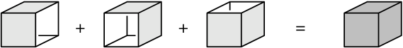
Figure 8: The three ribbons that build the surface of the cube. Each face of the cube is covered exactly twice by plaquettes from two ribbons corresponding to different coordinate planes.

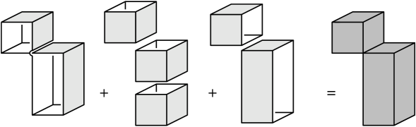
Figure 9: Example how a surface with one link of self-intersection is composed from ribbons. Each plaquette of the surface is covered twice by ribbons corresponding to different coordinate planes.

When one sums over all loops in all coordinate planes, all possible surfaces $\sigma$ on the dual lattice are summed over. Since each plaquette is covered twice by the ribbons, the factor $t$ is counted twice, giving the overall factor $t^{2|\sigma|}$, where $|\sigma|$ denotes the area of the surface. The factor $(-1)^{n(\gamma_{12})+n(\gamma_{13})+n(\gamma_{23})}$ turns into $(-1)^{L(\sigma)}$, where $L(\sigma)$ is the number of links where the surface self-intersects. The final result for the 3-$D$ partition function is

$$Z\;=\;\sum_{\sigma\in{\cal S}_{int}}(-1)^{L(\sigma)}\;t^{2|\sigma|}\;.$$ (3.18)

The set ${\cal S}_{int}$ are the surfaces which can be obtained by wrapping ribbons corresponding to the subset of loops in ${\cal L}_{int}$ onto each other. More explicitly the surfaces in ${\cal S}_{int}$ are closed, not necessarily connected surfaces, which are allowed to self-intersect, but plaquettes may not touch each other.

We remark, that when the set of loops in ${\cal L}_{int}$ is extended, so is the class of allowed surfaces in ${\cal S}_{int}$. For example if loops, where links can be occupied several times, are taken into account, one can generate surfaces where plaquettes of the surface touch each other. However, they are no longer necessarily closed surfaces. Consider e.g. the loop depicted in Fig. 2 (c). It gives rise to a ribbon where each of the plaquettes is covered twice, and the contribution thus survives summing over the auxiliary fields $A_{\mu\nu}(x)$. The corresponding surface has however a boundary. Thus as in the 2-$D$ case it is possible to allow for a larger class of surfaces than $S_{int}$. Many of these surfaces, such as our example of the doubly covered ribbon have no counterparts in the set ${\cal S}_{ext}$ of surfaces with extrinsic geometry and get cancelled. All these more general sets of surfaces can be generated by allowing for generalized sets of loops ${\cal L}_{int}$. In other words, the surfaces are classified by the behavior of the loops which are obtained as an intersection of the surfaces with all possible coordinate planes on the lattice. This makes (LABEL:surf1) and (3.18) very powerful for a simple characterization of possible classes of surfaces with intrinsic geometry. For all these cases the geometry factor is $(-1)^{L(\sigma)}$ and the partition function is given by (3.18).

3.3 Correlation functions in terms of surfaces

In this section we derive a simple formula for 2$n$-point functions in terms of surfaces. We will compute these correlation functions by making use of the variable bond Ising model,

$$Z\Big{(}\{\beta_{\langle x,y\rangle}\}\Big{)}\;=\;\sum_{\{s(x)=\pm 1\}}\exp\left(\sum_{\langle x,y\rangle}\beta_{\langle x,y\rangle}s(x)s(y)\right)\;.$$ (3.19)

This expression can serve as a generating functional for 2-point functions (or more general 2n-point) functions: Let 0 and z be the two lattice sites where the spins in the 2-point function are located. Connect them by an arbitrary set of links, $\Gamma$, forming a path from $0$ to $z$. It is convenient to encode the path $\Gamma$ by the set of directions $\hat{\mu}_{1}\dots\hat{\mu}_{|\Gamma|}$ which trace it out when starting at 0 (here $|\Gamma|$ denotes the length of $\Gamma$.) Then one can write,

$$\langle s(0)s(z)\rangle = \langle s(0)\underbrace{s(\hat{\mu}_{1})s(\hat{\mu}_{1})}_{=1}\dots\underbrace{s(z-\hat{\mu}_{|\Gamma|})s(z-\hat{\mu}_{|\Gamma|})}_{=1}s(z)\rangle=$$

$$\Big{\langle}\prod_{\langle x,y\rangle\in\Gamma}\!\!s(x)s(y)\Big{\rangle} = \frac{1}{Z}\left(\prod_{\langle x,y\rangle\in\Gamma}\frac{\partial}{\partial\beta_{\langle x,y\rangle}}\right)Z\Big{(}\{\beta_{\langle x,y\rangle}\}\Big{)}\Big{|}_{\beta_{\langle x,y\rangle}=\beta}\;.$$

We remark that it is not necessary to set the coupling constants equal (this was done only for notational convenience), and all results below can easily be generalized to the variable bond model. Also, the generalization to 2$n$-point functions is straightforward: simply replace the single path $\Gamma$ by a network of paths, consisting of links on the lattice, which connect all sites occuring in the 2$n$-point function. We will show in the end, that the result is independent of the choice of the network.

The essential step is to replace the partition function of the variable bond model by the corresponding expression in terms of surfaces. For notational convenience we will work with the representation in terms of surfaces with extrinsic geometry rather than the more cumbersome intrinsic geometry. However, it is of course possible to express the final result in terms of surfaces with intrinsic geometry. For the variable bond model the surface representation is given by,

$$Z\Big{(}\{\beta_{\langle x,y\rangle}\}\Big{)}\;=\;2\exp\left(\sum_{\langle x,y\rangle}\beta_{\langle x,y\rangle}\right)\sum_{\sigma\in{\cal S}_{int}}\;\prod_{\langle x,y\rangle:\;\langle x,y\rangle\in\sigma^{*}}e^{-2\beta_{\langle x,y\rangle}}\;.$$ (3.21)

Here $\sigma^{*}$ denotes the set of links dual to the plaquettes of $\sigma$. A straightforward but lengthy calculation gives

$$\prod_{\langle x,y\rangle\in\Gamma}\frac{\partial}{\partial\beta_{\langle x,y\rangle}}Z\Big{(}\{\beta_{\langle x,y\rangle}\}\Big{)}\Big{|}_{\beta_{\langle x,y\rangle}}\;=\;Z\;+$$

$$2e^{\beta 3V}(-2)\;\sum_{\langle x,y\rangle\in\Gamma}\;\;\;\sum_{\{\sigma:\;\langle x,y\rangle\in\sigma^{*}\}}\!\!\!\!\!\!\!e^{-2\beta|\sigma|}\qquad+$$

$$2e^{\beta 3V}(-2)^{2}\sum_{\langle x,y\rangle<\langle x^{\prime},y^{\prime}\rangle\in\Gamma}\;\;\sum_{\{\sigma:\;\langle x,y\rangle,\langle x^{\prime},y^{\prime}\rangle\in\sigma^{*}\}}\!\!\!\!\!\!\!\!\!\!\!\!\!e^{-2\beta|\sigma|}\qquad+$$

$$2e^{\beta 3V}(-2)^{3}\!\!\sum_{\langle x,y\rangle<\langle x^{\prime},y^{\prime}\rangle<\langle x^{\prime\prime},y^{\prime\prime}\rangle\in\Gamma}\;\;\;\;\sum_{\{\sigma:\;\langle x,y\rangle,\langle x^{\prime},y^{\prime}\rangle,\langle x^{\prime\prime},y^{\prime\prime}\rangle\in\sigma^{*}\}}\!\!\!\!\!\!\!\!\!\!\!\!\!\!\!\!\!\!\!\!\!\!\!e^{-2\beta|\sigma|}\quad+$$

$$\dots\dots$$

$$2e^{\beta 3V}(-2)^{|\Gamma|}\sum_{\{\sigma:\;|\Gamma\cap\sigma^{*}|=|\Gamma|\}}\!\!\!e^{-2\beta|\sigma|}\;.$$ (3.22)

We introduced an (arbitrary) ordering $\langle x,y\rangle<\langle x^{\prime},y^{\prime}\rangle\dots$ of the links in $\Gamma$. In the last term we introduced $|\Gamma\cap\sigma^{*}|$ to be the number of links in $\Gamma$ which are also in $\sigma^{*}$. The final step is to interpret all the contributions in terms of surfaces. Let $\sigma$ be a surface that intersects $\Gamma$ at $m$ links, then $\sigma$ is counted in the first $m+1$ terms on the right hand side of (3.22). To begin with, $\sigma$ is certainly counted in $Z$, which is the first term on the right hand side of (3.22), with a factor $1=(-2)^{0}{m\choose 0}$. Of course, there is also the factor $2\exp(\beta[3V-2|\sigma|])$ but this will appear in all terms in (3.22), so we will neglect it for the moment. In the second term in (3.22) the surface $\sigma$ gets firstly an overall factor of $-2$ and then it is counted $m$-times, since the first sum in this term runs over all links. Thus, in the second term of (3.22) $\sigma$ acquires the factor $(-2)m=(-2){m\choose 1}$. In the third term the overall factor is $(-2)^{2}$ and since the links in the sum are ordered the surface occurs ${m\choose 2}$ times. Thus the factor is $(-2)^{2}{m\choose 2}$. In general a surface which intersects $\Gamma$ at $m$ links obtains a factor of $(-2)^{i-1}{m\choose i-1}$ from the $i$-th term in (3.22). These factors can be summed up to give

$$\sum_{i=1}^{m+1}{m\choose i-1}(-2)^{i-1}\;=\;(1-2)^{m}\;=\;(-1)^{m}\;.$$

We thus end up with the surprisingly simple result (the overall factor $2e^{\beta 3V}$ gets cancelled when dividing by $Z$)

$$\langle s(x_{1})s(x_{2})\dots s(x_{2n})\rangle\;=\;\sum_{\sigma\in{\cal S}_{ext}}(-1)^{|\Gamma\cap\sigma^{*}|}\;\;t^{2|\sigma|}\;\Bigg{/}\;\sum_{\sigma\in{\cal S}_{ext}}t^{2|\sigma|}\;,$$ (3.23)

where $\Gamma$ is an arbitrary network of paths connecting the sites $x_{1},\dots x_{2n}$ and $t$ denotes $\exp(-\beta)$. It is simple to see the independence of (3.23) from the choice of $\Gamma$: The network $\Gamma$ can be deformed arbitrarily by adding single plaquettes to $\Gamma$ and since a plaquette always intersects an even number of times (0, 2 or 4-times) with a given surface, the intersection term $(-1)^{|\Gamma\cap\sigma^{*}|}$ remains invariant under such deformations. We finally remark, that the same formula holds if one works with the representation in terms of surfaces with intrinsic geometry (certainly the self-intersection factor $(-1)^{L(\sigma)}$ has to be re-inserted). The formula also holds in 2-$D$, when the surfaces $\sigma$ are replaced by the loops $\gamma$.

4 Discussion

In this paper we discussed the hopping expansion of the Grassmann representation of the Ising model in both 2 and 3 dimensions. For the 3-$D$ case an auxiliary field was introduced in order to write the action in quadratic form. In both dimensions the expansion was interpreted in terms of loops or surfaces. It was shown that the hopping expansion, with its calculus of hopping generators, provides an exact algebraic representation of the expansions in terms of loops and surfaces, respectively. This connection allows for a simple algebraic treatment of many of the problems which emerge in the loop or surface expansion and are rather intractable when working with the original geometrical objects.

Counting problems and symmetry factors can be analyzed in a rather simple fashion using the algebraic representation. As an application, in 2-$D$, we gave the corrected result of the loop representation of the free energy and computed its radius of convergence showing that it is determined by the critical temperature. In 3-$D$ we derived a representation of the partition function as a product of 2-$D$ Ising models in their loop representation coupled to an auxiliary field. We gave a simple proof that the self intersection factor leads to the cancellations necessary so that the sum over surfaces with intrinsic geometries reproduces the correct partition function. The possible classes of surfaces to be summed over were characterized by their intersections with all coordinate planes of the lattice. Our formula for the $2n$-point functions in terms of surfaces illustrates the tight relation between dynamics and geometry in 2- and 3-dimensional Ising models.

The fermionic representation of the Ising model is also known in dimensions higher than 3. It involves however terms of order larger than the quartic contributions generating the plaquettes in 3-$D$. By introducing several auxiliary fields one could write the action as a quadratic form and perform the hopping expansion along the lines of this paper. However, the geometrical interpretation of the emerging structures might turn out to be rather involved.

The results obtained here might have a more or less straightforward generalization to other models where Grassmann representations exist [7], such as vertex models and the Ashkin-Teller model. It would be interesting to work out representations of these models in terms of geometrical objects with intrinsic geometry. In particular representations of $n$-point functions in terms of these surfaces could be analyzed further. The outcome of such an enterprise might be a better understanding of the relation between dynamics and geometrical concepts.

Acknowledgement: This work is supported in part by NSERC of Canada, NATO CRG 970561 and the Fonds zur Förderung der Wissenschaftlichen Forschung in Österreich under project number J1577-PHY.

References

- [1]
- [2] M. Kac and J.C. Ward, Phys. Rev. 88 (1952) 1332.
- [3] R.B. Potts and J.C. Ward, Prog. Theor. Phys. 13 (1955) 38.
- [4] S. Sherman, J. Math. Phys. 1 (1961) 202; J. Math. Phys. 4 (1963) 1213.
-
[5]
L.D. Landau and E.M. Lifshitz,
Statistical Mechanics, Pergamon Press, New York, 1959;
R.P. Feynman, Statistical Mechanics, Benjamin Publishers, Reading, MA, 1972. - [6] E. Fradkin, M. Srednicki and L. Susskind, Phys. Rev. D 21 (1980) 2885.
- [7] S. Samuel, J. Math. Phys. 21 (1980) 2806; 2815.
- [8] S. Samuel, J. Math. Phys. 21 (1980) 2820.
- [9] C. Itzykson, Nucl. Phys. B210 (1982) 448.
- [10] C. Itzykson, Nucl. Phys. B210 (1982) 477.
- [11] Vi.S. Dotsenko and Vl. S. Dotsenko, Adv. Phys. 32 (1983) 129.
- [12] A.R. Kavalov and A.G. Sedrakyan, Nucl. Phys. B 285 (1987) 264.
-
[13]
A. Sedrakyan,
Phys. Lett.
137 B (1984) 397;
A. Kavalov and A. Sedrakyan, Phys. Lett. 173 B (1986) 449. - [14] A. Casher, D. Foerster and P. Windey, Nucl. Phys. B 251 (1985) 29.
- [15] P. Orland, Phys. Rev. Lett. 59 (1987) 2393.
- [16] J. Distler, Nucl. Phys. B 388 (1992) 648.
- [17] A. Polyakov, Phys. Lett. 82B (1979) 247; 103B (1981) 211.
-
[18]
Vl. Dotsenko and A. Polyakov,
in Advanced Studies in Pure Mathematics
15;
Vl. Dotsenko, Nucl. Phys. B285 (1987) 45. - [19] I. Montvay and G. Münster, Quantum Fields on a Lattice, Cambridge University Press, Cambridge, 1994.