ABOUT
SYMMETRIES IN PHYSICS

Abstract

The goal of this introduction to symmetries is to present some general ideas, to outline the fundamental concepts and results of the subject and to situate a bit the following lectures of this school. [These notes represent the write-up of a lecture presented at the fifth Séminaire Rhodanien de Physique “Sur les Symétries en Physique” held at Dolomieu (France), 17-21 March 1997. Up to the appendix and the graphics, it is to be published in Symmetries in Physics, F. Gieres, M. Kibler, C. Lucchesi and O. Piguet, eds. (Editions Frontières, 1998).]

LYCEN 9754

December 1997

Institut de Physique Nucléaire de Lyon, IN2P3/CNRS, Université Claude Bernard
43, boulevard du 11 novembre 1918, F - 69622 - Villeurbanne CEDEX

Contents

1   Introduction 1

2   Symmetries of geometric objects 2

3   Symmetries of the laws of nature 5

1   Geometric (space-time) symmetries 6

2   Internal symmetries 10

3   From global to local symmetries 11

4   Combining geometric and internal symmetries 14

5   Duality symmetries 15

6   Miscellaneous 16

4   The mathematical description of symmetries and their implementation in physical theories 16

1   Mathematical description : (Lie) groups and algebras 16

2   Physical implementation : representations 18

3   Generalizations 18

5   Implications of symmetries for the formalism, the results and the structure of physical theories 20

6   Different manifestations of symmetries 22

1   Broken symmetries 23

2   Miscellaneous and some important asymmetries 26

7   Conclusion 27

A.1   On (Lie) groups and algebras 28

A.2   About representations 32

1 Introduction

‘Symmetric’ objects are aesthetically appealing and fascinating for the human mind. But what does symmetric mean? The original sense of the Greek word symmetros is ‘well-proportioned’ or ‘harmonious’. In his classic work on symmetry [1], H. Weyl puts it the following way : “Symmetry denotes that sort of concordance of several parts by which they integrate into a whole. Beauty is bound up with symmetry.” This fact might account for the omnipresence of symmetries in nature and our description of it, if we adhere to the views of d’Arcy Thompson [2] : “The perfection of mathematical beauty is such that whatever is most beautiful and regular is also found to be most useful and excellent.”

In less poetic terms (and with a thought for the great cathedral builders of the Renaissance), we could say that stable complex systems are best created by assembling in a regular way symmetric constituents blocks. Thus, it is natural that symmetries manifest themselves at all levels - microscopic and macroscopic - in our world as we see it, as we comprehend it and as we shape it.

Outline of the notes

These notes are intended to be of an elementary level, though some remarks refer to some more specific knowledge of physics or mathematics. (For the more technical parts of the notes, I assume some familiarity with the algebraic tools of the subject which the reader should remember from quantum mechanics : these are the notions of group, Lie group, Lie algebra and the representations of these algebraic structures. These concepts are briefly reviewed in section 4 and for the reader’s convenience, we have summarized the basic definitions together with some illustrative examples in an appendix.) In my write-up, I have preferred to maintain the informal character of the lectures rather than making attempts for formal rigor.

In the next two sections, we successively define and classify symmetries of geometric objects in space (which may be referred to as spatial symmetries) and symmetries of the laws of nature (physical symmetries). In section 4, we recall how symmetries are described in mathematical terms (groups, algebras,…) and how these mathematical structures are implemented in physical theories (representations,…). Thereafter, it is shown how the presence of symmetries affects physics at different levels : the formalism, the predictions and the general structure of theories. In conclusion, different manifestations of symmetries are indicated (approximate symmetries, broken symmetries,…).

About the literature

Though I tried to convey a flavor of the subject, it was neither possible nor intended to present an exhaustive treatment of it. For further information, the interested reader is referred to the many excellent and fascinating textbooks which are largely or completely devoted to symmetries : a selection of them is given in the bibliography [4]-[21]. We particularly mention the wonderful introductions to symmetries given by H. Weyl [1] and R. Feynman [4] in series of lectures addressed towards a general audience. In preparing these notes, I repeatedly used the books of Tarassow [5] and Genz/Decker [6] which I recommend wholeheartedly together with the pleasant and somewhat encyclopedic monograph of Sivardière [7] (though I am afraid none of these texts is available in English …).

2 Symmetries of geometric objects

In everyday life, symmetry usually means left-right (mirror or bilateral) sym- metry. For an object in a plane, this means that there exists a symmetry line and for an object in space, it amounts to the existence of a symmetry plane: if you exchange the two sides of the object, it looks exactly the same. This symmetry is realized - at least approximatively - for human beings and higher animals. (Henceforth, it is also the first symmetry of which we became aware in our personal life.)

One may wonder whether there is any reason for the occurrence of this symmetry for humans and animals. Obviously, there are two preferred directions for all of these beings : on one hand, there is the direction of motion (which is used when looking for food, attacking the enemy or joining friends) and on the other hand, there is the direction of gravity to which everybody is subject to. Altogether these two directions define a plane of symmetry in space.

What can we learn from these simple reflections? They show that symmetries usually reflect some intrinsic properties or characteristics of objects and of the space to which they belong. And they indicate that symmetries in nature are often realized as nearby (approximate) symmetries rather than in an exact way. It should be noted that, in general, symmetries in the living nature only manifest themselves if they are privileged from the point of view of selection [8].

The interpretation of our initial example is confirmed by looking at the plant world : for plants and trees, there is only one distinguished direction, namely the one given by gravity, all horizontal directions being equally well suited for absorbing oxygen, light or humidity. Consequently, plants and trees admit one symmetry axis and thus have rotational symmetry. Trees with many branches approximately have a continuous rotational symmetry around the vertical axis of their trunk, while flowers rather have a discrete rotational symmetry. In fact, many flowers have five petals and therefore admit a discrete rotational symmetry of fifth order : they are transformed into themselves when turned by an angle $n\,{360^{\circ}\over 5}\ ({\rm with}\;n\in{\bf Z})$ around their symmetry axis.

Again one may wonder whether there is a deeper reason for this symmetry of order five that many flowers share? Simple models for the growth of flowers show that the number of petals is a Fibonacci number ($1,2,3,5,8,13,..$) [22]. (Such models also explain the manifestation of these numbers in the symmetric arrangement of sunflowers seats or of branches around the stem of a tree,…) Should you notice many flowers with six petals on your next outdoor trip, then you should not conclude that the models we mentioned are wrong : the growth conditions for the buds of these flowers are different and such that their petals get organized as two generations of $3$ petals each, $3$ being a Fibonacci number too!

A very different and somewhat metaphysical argument in favor of the number $5$ is referred to in [5]. The five petals of a flower span a regular pentagon and if you try to put as many as possible of these together (i.e. pave or tile a plane with them), then some spaces will remain uncovered between these pentagons - see figure below. In fact, such a tiling can be achieved with regular triangles, squares or hexagons, but not with pentagons. One can argue that by choosing a fifth-order symmetry, the flowers try to fight for survival and protect themselves against crystallization, the first step of which would consist of getting ‘trapped’ in a crystal lattice. Though this remark should not be taken too seriously, it reveals an important fact concerning symmetries in nature [23] :

Only certain symmetries are supported by the space in which we live.

This does not only apply to patterns created by men, but to all regular structures occurring in nature. (Our example of pentagons refers to planar domains, but we can also think about our three-dimensional space : there are only five Platonic bodies, i.e. regular polyeders like the cube or tetraeder.) Even the mathematical tools we use to describe physical phenomena are reflections of the symmetries of space. For instance, the Pythagorean theorem would not hold as such if space were to have other symmetries.

The issue of tilings brings us to the subject of symmetries in art [18], e.g. the famous tilings of the Alhambra, ornamental symmetry, Escher’s drawings [19], Penrose tilings [7],… The construction of these regular patterns is based on translational symmetry and combinations of all spatial symmetries introduced so far.

The paradigm, or perfect example, of symmetries is definitely given by the crystal. For a discussion of regular and quasicrystals, we refer to [7, 24] and the lectures of J.P. Gazeau in this volume.

After contemplating all these examples, the reader may still wonder :

What is a symmetry?

Roughly speaking, an object is symmetric (has a symmetry) if there is something you can do to it, so that after you finished doing it, it looks exactly the same way it did before. In other words, a symmetry transformation of a geometric object (which is part of a plane or of space) is a transformation of the object whose realization (effect) is impossible to detect. For instance, for the following geometric figures, it is not possible to notice the effect of a rotation by an angle of, respectively, $180^{\circ}$, $90^{\circ}$ or an arbitrary value around their symmetry axis.

The more symmetries an object admits, the more symmetric it is.

In order to formulate these ideas more precisely from the mathematical point of view [25, 21], we recall that an isometry of a geometric object in Euclidean space is a transformation of it which preserves the distances. Examples are given by rotations, translations or reflections.

Definition 1

A symmetry or symmetry transformation of a geometric object in Euclidean space is an isometry which maps the object onto itself. If an object admits a certain symmetry, it is said to have this invariance.

The set of all symmetry transformations of an object represents a group (the group multiplication being the consecutive application of transformations) : this is the symmetry group of the object.

3 Symmetries of the laws of nature

We can fit the definition given for objects in space to the present case: loosely speaking, a symmetry of a law of nature means that there is something we can do to a physical law - or rather to our way of representing it - which makes no difference and leaves everything unchanged in its effects. To be more precise, we consider a physical system described by a law or, more specifically, by some equations involving a certain number of variables which may (or may not) represent directly observable quantities, and which possibly depend on the space-time coordinates. E.g. we consider the propagation of an impulse with the speed of light $c$, as described by the equation $\Box\varphi(\vec{r},t)=0$ where $\Box\equiv{1\over c^{2}}\,\partial_{t}^{2}-(\partial_{x}^{2}+\partial_{y}^{2}+\partial_{z}^{2})$ denotes the wave operator.

Definition 2

A symmetry transformation of a physical law is a change of the variables and/or space-time coordinates (in terms of which it is formulated) such that the equations describing the law have the same form in terms of the new variables and coordinates as they had in terms of the old ones. One says that the equations preserve their form or that they are covariant with respect to the sym- metry transformation.

Thus, the realization of a symmetry transformation is impossible to detect. In our example of the wave equation, we may apply a Lorentz transformation (a boost) with velocity $\vec{v}=(v,0,0)$ : under this operation, the space-time coordinates $(\vec{r},t)$ become

$$x^{\prime}=\gamma(x-vt)\quad,\quad y^{\prime}=y\quad,\quad z^{\prime}=z\quad,\quad t^{\prime}=\gamma(t-{v\over c^{2}}x)\ \ ,$$ (3.1)

where $\gamma=(1-v^{2}/c^{2})^{-1/2}$, but the wave operator is invariant under these transformations, i.e. $\Box^{\prime}=\Box$. This result, first found by H. Lorentz, and the fact that the scalar function $\varphi$ has the same numerical value in the transformed and original reference frames, i.e. $\varphi^{\prime}(\vec{r}^{\,\prime},t^{\prime})=\varphi(\vec{r},t)$, imply that the wave equation has exactly the same form in both reference frames. In physical terms: the wave propagates in the same way and with the same velocity $c$ in two inertial frames that are in uniform motion relative to each other. With another phrasing we can say that, by analyzing the wave propagation in a spaceship, an observer cannot tell whether this spaceship is at rest or in uniform motion relative to the stars (unless he looks outside of its windows).

In the next sections, we will be concerned with physics in flat, four-dimen- sional space-time. Curved space and symmetries in other-dimensional spaces, which are relevant for statistical mechanics or string theory, will only be commented upon.

For the classification of symmetries, one distinguishes between those which operate on space-time coordinates, the so-called geometric symmetries and those which do not affect them, the internal symmetries.

3.1 Geometric (space-time) symmetries

The basic operations are the following ones [26] :

$$\begin{array}[]{ll}\mbox{Translation in time :}&\,t^{\prime}=t+a^{0}\\ \mbox{Translation in space :}&\vec{r}^{\,\prime}=\vec{r}+\vec{a}\\ \mbox{Rotation in space :}&\vec{r}^{\,\prime}=R\,\vec{r}\ \ ,\end{array}$$ (3.2)

where $a^{0}\in{\bf R},\ \vec{a}\in{\bf R}^{3}$, $R$ being a $3\times 3$ rotation matrix. These transformations preserve the form of time evolution equations, e.g. of the equation $m\ddot{\vec{r}}=\vec{0}$ in classical mechanics. (Thus, some potential symmetries for objects in space are basic symmetries of the laws of nature.) The origin of these fundamental invariances can be traced back to intrinsic properties of space and time - see the table below.

Since the changes of coordinates (3.2) are continuous symmetry transformations in the sense that they are parametrized in a smooth way by real numbers, we can apply the famous theorem of E. Noether :

Covariance of the equations of motion with respect to a continuous transformation with $n$ parameters implies the existence of $n$ conserved quantities (‘conserved charges’ or ‘integrals of motion’), i.e. it implies conservation laws.

We have the following correspondence in the present case :

Property	Invariance of equations	Conserved quantity
homogeneity of time	time translation invariance	energy
homogeneity of space	translational invariance	momentum
isotropy of space	rotational invariance	angular momentum

In non-relativistic theories like Newtonian mechanics or usual quantum mechanics, the time evolution equations are also covariant with respect to the Galilean transformation

$$\vec{r}^{\,\prime}=\vec{r}-\vec{v}\,t\qquad{\rm where}\ \;\vec{v}\in{\bf R}^{3}\ \ .$$ (3.3)

In relativistic theories like electromagnetism, this symmetry transformation is to be replaced by the Lorentz transformation (3.1).

In order to discuss the relativistic symmetries from a formal point of view, it is convenient to introduce Minkowski space $({\bf R}^{4},(ds)^{2})$, i.e. the real vector space ${\bf R}^{4}$ parametrized by space-time coordinates $x=(x^{\mu})_{{\mu}=0,1,2,3}=(ct,\vec{r}\,)$ and equipped with the metric

$$(ds)^{2}=(dx)^{2}\equiv c^{2}dt^{2}-(d\vec{r}\,)^{2}\ \ .$$ (3.4)

By definition, the Lorentz group $L$ is the set of all real $4\times 4$ matrices $\Lambda$ which leave the Minkowski metric (3.4) invariant, i.e. all linear coordinate transformations $x\to x^{\prime}=\Lambda x$ such that $(dx^{\prime})^{2}=(dx)^{2}$. These include the rotations and Lorentz boosts, but also the operations of parity ($\vec{r}^{\,\prime}=-\vec{r}\,$) and time reversal ($t^{\prime}=-t$) [27]. The latter transformations are referred to as discrete - as opposed to continuous - symmetries.

The space-time translations $x\to x+a$ also leave the Minkowski metric invariant, because $d(x+a)=dx$. They form a group, the group of translations ${\cal T}_{4}$, i.e. the set of all mappings $T_{a}$ (with $a=(a^{0},\vec{a}\,)\in{\bf R}^{4}$ ) defined by

$$T_{a}\ :\ {\bf R}^{4} \longrightarrow\ {\bf R}^{4}$$

$$x \longmapsto\ T_{a}(x)=x+a\ \ ,$$

the group multiplication being the composition : $T_{a}\circ T_{b}=T_{a+b}$. By combining Lorentz transformations and translations, we obtain the Poincaré group

$$P=L\subset\!\!\!\!\!\!\times{\cal T}_{4}\ \ ,$$ (3.5)

whose elements $(\Lambda,T_{a})$ act on $x\in{\bf R}^{4}$ according to $x\to\Lambda x+a$. They represent isometries of Minkowski space.

An elementary particle is an object whose nature does not change when it is translated in space or time, when it is rotated or seen from an observer in uniform motion relative to it. These considerations led E. Wigner to postulate that the quantum mechanical states of such a particle should belong to a Hilbert space carrying a certain representation of the Poincaré group (cf. appendix A.2). Thus, the very definition of an elementary particle is based on the geometric symmetries and so is the whole classification of particles according to their mass and spin [28]. A particle may be viewed as the ‘quantum’ of a classical relativistic field $(A_{1}(x),...,A_{n}(x))$, i.e. a collection of space-time functions $A_{i}(x)$ having specific transformation properties with respect to Poincaré transformations. The way in which these fields can interact with each other, is strongly restricted by the requirement of relativistic covariance of the equations of motion. In summary :

The Poincaré group is an invariance group of all relativistic theories and thereby determines their general structure to a large extent.

It should be noted that continuous symmetries in physics are often formulated in terms of infinitesimal rather than finite transformations, i.e. one considers the Lie algebra rather than the Lie group of transformations - see the appendix for an illustration concerning rotations.

One may wonder whether there are more general groups (or algebraic structures) containing the Poincaré group as a subgroup, which are of physical interest. Indeed, there are such extensions of the Poincaré group, two of which will now be presented.

3.1.1 The conformal group

Conformal transformations of Minkowski space are coordinate transformations $x\to x^{\prime}(x)$ which are such that the induced change of the metric is a rescaling by a positive function :

$$(ds^{\prime})^{2}={\rm e}^{\Omega(x)}\;ds^{2}\ \ ,$$ (3.6)

where $\Omega$ is a smooth, real-valued function. Geometrically, this means that a conformal transformation preserves the angles in magnitude and direction, though it may locally change the distances in a smooth way. Of course, transformations with this property are essential for the design of geographic maps ; remarkably enough, it was already realized by Ptolemy that the stereographic projection of a sphere onto a plane represents a conformal mapping.

The set of all conformal transformations of Minkowski space is called its conformal group. Of course, this group contains the Poincaré transformations for which $\Omega=0$. But it also involves dilatations (rescalings or scale transformations) by a positive, constant factor ${\rm e}^{\lambda}$ :

$$x^{\prime}={\rm e}^{\lambda}\,x\ \ \Longrightarrow\ \ (ds^{\prime})^{2}={\rm e}^{\lambda}\;ds^{2}\ \ .$$

Besides, it contains the so-called special conformal transformations [29].

Conformal field theories, i.e. field theories admitting the conformal group as symmetry group have been intensively studied during the last decades. Their relevance for particle physics is severely limited by the fact that the presence of a massive particle in such models implies the existence of a continuous mass spectrum [30]. However, scale transformations play an important rôle for the description of critical phenomena (phase transitions) in statistical physics [31]. Furthermore, two-dimensional conformal field theories [32] are at the very heart of string theories which are currently viewed as the most promising candidates for a unified quantum theory of all fundamental interactions of nature [33].

3.1.2 The super Poincaré algebra

Let ${\rm Lie}\,P$ denote the Lie algebra associated to the Poincaré group, i.e. the set of infinitesimal translations, rotations and boosts. The super Poincaré algebra

$${\cal G}_{\overline{0}}\oplus{\cal G}_{\overline{1}}\ \equiv\ {\rm Lie}\,P\ \oplus\{{\rm SUSY}\}$$ (3.7)

is a Lie superalgebra (or ${\bf Z}_{2}$-graded Lie algebra) which roughly means the following [34, 35]. The elements of the vector spaces ${\cal G}_{\overline{0}}$ and ${\cal G}_{\overline{1}}$ are assigned a degree or parity $0$ and $1$, respectively : therefore, they are referred to as even and odd or as bosonic and fermionic elements, respectively, and one often writes ${\cal B}={\cal G}_{\overline{0}}$ and ${\cal F}={\cal G}_{\overline{1}}$. Instead of the usual Lie commutator $[A,B]\equiv AB-BA$, one has a ‘${\bf Z}_{2}$-graded’ commutator $[A,B\}$ which has the properties of an anticommutator $\{A,B\}\equiv AB+BA$ if $A$ and $B$ are both fermionic and otherwise those of a commutator. Schematically, one has

$$\framebox{\mbox{$\ {[{\cal B},{\cal B}]}={\cal B}\quad,\quad{[{\cal B},{\cal F}]}={\cal F}\quad,\quad\{{\cal F},{\cal F}\}={\cal B}\ $}}\ \ .$$ (3.8)

In our example of the super Poincaré algebra, the relation ${[{\cal B},{\cal B}]}={\cal B}$ summarizes the commutation relations of the Poincaré algebra ${\cal B}={\rm Lie}\,P$ and ${\cal F}=\{{\rm SUSY}\}$ is spanned by the so-called supersymmetry generators $(Q_{\alpha})_{\alpha=1,..,4}$: for these elements, the relation $\{{\cal F},{\cal F}\}={\cal B}$ takes the explicit form

$$\ \{Q_{\alpha},Q_{\beta}\}=\sum_{\mu=0}^{3}f_{\alpha\beta}^{\mu}\,P_{\mu}\$$ (3.9)

where $f_{\alpha\beta}^{\mu}\in{\bf C}$ are structure constants and $(P_{\mu})_{\mu=0,..,3}$ the generators of space-time translations (i.e. $P_{\mu}=i\partial_{\mu}$ in a representation by differential operators). In essence, the last relation states that

The supersymmetry generators are ‘square roots’ of translation generators.

By introducing $4N$ (with $N=2,3,...$ ) supersymmetry generators $Q_{\alpha}^{i}$ (where $i=1,..,N$), one can define the $N$-extended super Poincaré algebra.

Supersymmetric quantum mechanics [36] and supersymmetric field theories [35, 37] represent realizations of the super Poincaré algebra - see the lectures of V. Hussin, J.-P. Derendinger and H.P. Nilles in this volume : in the latter theories, the supersymmetry generators relate bosonic and fermionic fields and thus represent a symmetry between these fields.

3.2 Internal symmetries

As an example, we consider the time evolution of a free particle of mass $m$ and charge $e$ as described by quantum mechanics. It is governed by the Schrödinger equation

$$H\psi={\rm i}\hbar\,\partial_{t}\psi\ \ ,$$ (3.10)

where $H={1\over 2m}\,\vec{P}^{2}={1\over 2m}\,({\hbar\over{\rm i}}\,\vec{\nabla})^{2}$ denotes the Hamiltonian operator and $\psi=\psi(\vec{r},t)$ the wave function associated to the particle. Obviously, equation (3.10) is invariant under the global (i.e. $\vec{r}$ and $t$ independent) phase transformation

$$\psi\ \longmapsto\ \psi^{\prime}={\rm e}^{{\rm i}\alpha}\psi\ \ ,$$ (3.11)

where $\alpha\in{\bf R}$ is a constant. Note that ${\rm e}^{{\rm i}\alpha}$ is an element of the abelian Lie group $U(1)$ of complex numbers of modulus one.

We emphasize that the invariance (3.11) represents an internal symmetry: it only acts on the space of fields (i.e. space-time functions) $\psi$ and not on the space-time manifold.

According to Noether’s theorem, the invariance of the equation of motion under the continuous symmetry (3.11) implies the existence of a conserved charge. In fact, one can easily check that the integral $\int_{{\bf R}^{3}}|\psi(\vec{r},t)|^{2}\,d^{3}x$ (which may be associated with the electric charge of the particle) does not depend on the variable $t$ if $\psi$ is a solution of (3.10).

3.3 From global to local symmetries

We now consider a local (i.e. $\vec{r}$ and $t$ dependent) phase transformation or so-called gauge transformation :

$$\framebox{\mbox{$\ \psi^{\prime}(\vec{r},t)={\rm e}^{{\rm i}\alpha(\vec{r},t)}\,\psi(\vec{r},t)\ $}}\qquad{\rm with}\quad\alpha(\vec{r},t)\in{\bf R}\ \ .$$ (3.12)

The Schrödinger equation (3.10) is not invariant under these transformations. To verify this fact explicitly, we introduce relativistic notation (and choose a system of units in which the velocity of light $c$ equals one) : for the derivatives $(\partial_{\mu}\psi)\equiv(\partial\psi/\partial x^{\mu})=(\partial_{t}\psi,\vec{\nabla}\psi)$ with respect to the space-time coordinates $(x^{\mu})_{\mu=0,..,3}=(t,\vec{r}\,)$, we have

$$\partial_{\mu}\psi^{\prime}={\rm e}^{{\rm i}\alpha}[\partial_{\mu}\psi+{\rm i}(\partial_{\mu}\alpha)\psi]$$

and the terms in $\partial_{\mu}\alpha$ do not drop out of the primed (i.e. gauge transformed) Schrödinger equation. Thus, if we want the gauge transformations (3.12) to be a symmetry of the theory, we have to modify the evolution equation (3.10) in such a way that it preserves its form under these transformations. For this purpose, we introduce some new fields into the equation which transform in a specific way so as to ensure its covariance. The simplest way to realize this idea consists of introducing a scalar potential $\phi(\vec{r},t)$ and a vector potential $\vec{A}(\vec{r},t)$ into the free Schrödinger equation by means of the so-called minimal coupling procedure: one replaces the ordinary derivative by the (gauge-) covariant derivative,

$$\partial_{\mu}\ \longrightarrow\ \ \framebox{\mbox{$\ D^{(A)}_{\mu}\equiv\partial_{\mu}+\displaystyle{{\rm i}e\over\hbar}\,A_{\mu}\ $}}\qquad{\rm where}\quad(A_{\mu})\equiv(\Phi,-\vec{A})\ \ ,$$ (3.13)

i.e. explicitly $\partial_{t}\rightarrow\partial_{t}+{{\rm i}e\over\hbar}\Phi,\ \vec{\nabla}\rightarrow\vec{\nabla}-{{\rm i}e\over\hbar}\vec{A}$. Furthermore, the gauge vector field $(A_{\mu})$ is required to transform inhomogenously under gauge transformations,

$$\framebox{\mbox{$\ A_{\mu}^{\prime}=A_{\mu}-\displaystyle{\hbar\over e}\,\partial_{\mu}\alpha\ $}}\qquad\Longleftrightarrow\ \ \left\{\begin{array}[]{l}\Phi^{\prime}=\Phi-{\hbar\over e}\,\partial_{t}\alpha\\ \vec{A}^{\prime}=\vec{A}+{\hbar\over e}\,\vec{\nabla}\alpha\end{array}\right.\ \ ,$$ (3.14)

so as to compensate the unwanted terms in $\partial_{\mu}\alpha$ in the primed equation. In fact,

$$(D_{\mu}^{(A)}\psi)^{\prime}\equiv D_{\mu}^{(A^{\prime})}\psi^{\prime} = (\partial_{\mu}+\displaystyle{{\rm i}e\over\hbar}\,A_{\mu}^{\prime})\,({\rm e}^{{\rm i}\alpha}\psi)$$

$$= {\rm e}^{{\rm i}\alpha}\,\left[D_{\mu}^{(A)}\psi+{\rm i}(\partial_{\mu}\alpha)\psi-{\rm i}(\partial_{\mu}\alpha)\psi\right]\ \ ,$$

which means that the covariant derivative of $\psi$ transforms in the same way as $\psi$ (whence its name) :

$$\framebox{\mbox{$\ (D_{\mu}^{(A)}\psi)^{\prime}={\rm e}^{{\rm i}\alpha}\;D_{\mu}^{(A)}\psi\ $}}\ \ .$$ (3.15)

After performing the minimal coupling, the free Schrödinger equation becomes

$$-\displaystyle{\hbar^{2}\over 2m}\,(\vec{\nabla}-\displaystyle{{\rm i}e\over\hbar}\,\vec{A}\,)^{2}\psi\,=\,{\rm i}\hbar\,(\partial_{t}+\displaystyle{{\rm i}e\over\hbar}\,\Phi)\psi$$

or

$${1\over 2m}(\vec{P}-e\vec{A}\,)^{2}\psi+e\Phi\,\psi\,=\,{\rm i}\hbar\,\partial_{t}\psi\ \ .$$ (3.16)

This differential equation describes the coupling of the particle of mass $m$ and charge $e$ with the electromagnetic field associated to the potential $(A_{\mu})$,

$$\vec{E} \equiv -\stackrel{{\scriptstyle\rightarrow}}{{{\rm grad}}}\Phi-\partial_{t}\vec{A}$$ (3.17)

$$\vec{B} \equiv \stackrel{{\scriptstyle\rightarrow}}{{{\rm rot}}}\vec{A}\ \ .$$

By construction, the interacting Schrödinger equation (3.16) is invariant under the gauge transformations of $\psi$ and $A_{\mu}$ (which leave the field strengths $\vec{E},\vec{B}$ invariant).

Let us summarize once more the whole gauging procedure in quantum mechanics :

(1) The starting point is the Schrödinger equation for a free particle : it is invariant under global $U(1)$-transformations which implies the conservation of electric charge by virtue of Noether’s theorem. (2) The requirement that the Schrödinger equation be invariant under local $U(1)$-transformations (and simplicity) implies • the introduction of a gauge field $(A_{\mu})$ • that the way in which matter and gauge fields interact with each other is fixed !

Clearly, the fact that symmetries determine the (form of) interactions is a very strong result. The gauging recipe is at the origin of one of the greatest success stories of theoretical physics : the introduction of non-abelian gauge (Yang- Mills) theories led to the development of the standard model of particle physics [28, 38, 39]. After the foregoing discussion of quantum mechanics, it is straightforward to outline the construction of Yang-Mills theories. Instead of the abelian Lie group $U(1)$, one considers a non-abelian (and compact) Lie group $G$, e.g. the special unitary group

$$SU(n)=\{n\times n\;\mbox{matrices}\ A\ \mbox{with complex coefficients}\ |\;A^{\dagger}A={\bf 1}_{n},\,{\rm det}\,A=1\}.$$

Just as it was the case for quantum mechanics, the starting point (input) is the following :

1. A certain content of matter fields $\varphi_{1}(x),...,\varphi_{N}(x)$ (scalar or spinor fields) which are best assembled into a multiplet $\Phi=(\varphi_{1},...,\varphi_{N})^{t}$.

2. A continuous symmetry group $G$.

3. A Hamiltonian (or Lagrangian) which describes the dynamics and self-interaction of the fields $\varphi_{i}$ and which is invariant under global internal symmetry transformations $g\in G$, i.e. under

   $$g={\rm e}^{{\rm i}\underline{\alpha}}\qquad{\rm with}\ \;\underline{\alpha}=\sum_{a=1}^{{\rm dim}\,G}\alpha^{a}t_{a}\ \ ,$$

   where $\{t_{a}\}_{a=1,..,{\rm dim}\,G}$ denotes a basis of the Lie algebra of $G$ and $\alpha^{a}\in{\bf R}$. (We remark that $g$ acts on the multiplet $\Phi$ by means of an $N\times N$ representation matrix $D(g)$.)

The gauging procedure ($\alpha^{a}\to\alpha^{a}(x)$) then leads to the introduction of a gauge field with values in the Lie algebra of $G$,

$$\underline{A}_{\mu}(x)=\sum_{a=1}^{{\rm dim}\,G}A_{\mu}^{a}(x)t_{a}\ \ ,$$ (3.18)

transforming inhomogenously under $g(x)={{\rm e}}^{{{\rm i}}\underline{\alpha}(x)}$ :

$$\underline{A}_{\mu}^{\prime}=g^{-1}\,\underline{A}_{\mu}\,g+\displaystyle{{\rm i}\over\lambda}\;g^{-1}\,\partial_{\mu}g\qquad(\,\lambda=\mbox{coupling constant}\,)\ .$$ (3.19)

(Note that our previous equations are recovered for the case of the abelian group $U(1)$ for which ${\rm dim}\,G=1,\;t_{1}=1,\;\alpha^{1}\equiv\alpha$ and $\lambda=e/\hbar$.)

Gauge theories based on the groups $U(1),\,SU(2)$ and $SU(3)$ describe the electromagnetic, weak and strong interactions [28, 38] - see the lectures of P. Aurenche in this volume. The associated conserved charges are the electric charge, weak isospin and baryon number.

By gauging translations ($a^{\mu}\to a^{\mu}(x)$), one can construct general relativity which is invariant under the group of general coordinate transformations $x\to x^{\prime}(x)\simeq x+a(x)$. Similarly, by gauging rigid supersymmetry transformations, one obtains supergravity, i.e. the supersymmetric extension of general relativity [35]. Actually, general relativity was not constructed along these lines at first : Einstein derived his whole theory from a single symmetry principle, the equivalence principle (equivalence of inertial and gravitational mass) which finds its formal expression in the principle of general covariance (equivalence of all reference frames for the description of physical laws) [40]. For the interpretation of general relativity as a gauge theory, we refer to [41].

3.4 Combining geometric and internal symmetries

Let us recall that $SU(2)$ is a three-dimensional Lie group whose Lie algebra $su(2)$ is spanned by the Pauli matrices $(\sigma_{a})_{a=1,2,3}$. In field theories admitting $SU(2)$ as an internal symmetry group, one can introduce fields $\underline{\pi}(x)$ with values in the Lie algebra $su(2)$, i.e. $\underline{\pi}(x)=\sum_{a=1}^{3}\pi^{a}(x)\sigma_{a}$. For static configurations, the three components $\pi^{a}(\vec{r}\,)$ can be related to the three components of the ordinary space vector $\vec{r}=(x^{a})_{a=1,2,3}$, e.g. $\underline{\pi}^{a}(\vec{r}\,)=f(r)x^{a}$ where $r=\sqrt{(x^{1})^{2}+(x^{2})^{2}+(x^{3})^{2}}$, as in the Skyrme model of nuclear physics [42]. Similar examples are given by the monopole and instanton configurations which occur in $SU(2)$ gauge theories [39]. Thus, for these configurations (states), there is a certain mixing of indices associated with internal and geometric invariances (which are - a priori - completely unrelated).

One may wonder whether such a blend of internal and geometric symmetries may exist at a more fundamental level as a general feature of field theory and not simply in specific field configurations of particular models. (This feature would be very attractive for the construction of a unified theory of all fundamental interactions including gravity.) That this is not possible is expressed by the so-called no-go theorems, in particular the theorem of Coleman and Mandula, which essentially says the following : the most general invariance group of a relativistic quantum field theory is a direct product of the Poincaré group and an internal symmetry group, i.e. there is no mixture of these symmetry transformations.

However, these no-go theorems do not claim that such a mixture cannot exist if the set of all symmetry transformations represents a more general algebraic structure than a Lie group. Indeed, a famous result known as the theorem of Haag, Lopuszànski and Sohnius [35] states that the most general super Lie group of symmetries of a local field theory is the $N$-extended super Poincaré group in which there is a non-trivial mixing of geometric transformations and internal $SU(N)$ transformations. As a matter of fact, this result can also be viewed as a good argument in favor of the existence of supersymmetry as an invariance of nature since it states that supersymmetry is the natural (only possible) symmetry if one allows for super Lie groups as symmetry structures.

3.5 Duality symmetries

Let us consider Maxwell’s equations with both electric and magnetic sources (i.e. hypothetical magnetic monopoles) :

$${\rm div}\,\vec{E} = \rho_{e}\quad\,,\quad\stackrel{{\scriptstyle\rightarrow}}{{{\rm rot}}}\vec{E}+\partial_{t}\vec{B}\,=\,-\vec{\jmath}_{m}$$

$${\rm div}\,\vec{B} = \rho_{m}\quad,\quad\stackrel{{\scriptstyle\rightarrow}}{{{\rm rot}}}\vec{B}-\partial_{t}\vec{E}\,=\,\ \vec{\jmath}_{e}\ \ .$$ (3.20)

These equations are invariant under the duality transformation

$$(\vec{E},\vec{B},\rho_{e},\rho_{m},\vec{\jmath}_{e},\vec{\jmath}_{m})\longrightarrow(\vec{B},-\vec{E},\rho_{m},-\rho_{e},\vec{\jmath}_{m}-\vec{\jmath}_{e})\ \ .$$

In quantum mechanics, the presence of monopoles leads to the quantization of both electric and magnetic charges : for a given particle, these charges have to be related by Dirac’s condition $q_{e}q_{m}=2\pi n$ where $n$ denotes an entire number. Thus, the minimal charges obey $q_{m}={2\pi\over q_{e}}$. Since the duality symmetry exchanges electric and magnetic variables, we conclude from this relation that duality exchanges the coupling constant $q_{e}$ with its inverse (up to the factor $2\pi$) or that

Duality symmetries exchange weak and strong coupling regimes.

Henceforth, it is possible to learn about strong-coupling physics from the weak-coupling physics of a dual formulation of the theory [43]. Following a seminal paper by N. Seiberg and E. Witten, the latter idea proved to be extremely useful in recent years in the context of both field and string theories. It led to a further study of other extended objects like membranes or even higher-dimensional objects, all of which are referred to as $p$-branes ($p=1$ for strings, $p=2$ for two-dimensional membranes,…). All of these objects and theories seem to be related in amazing ways by duality transformations.

3.6 Miscellaneous

The fact that the rescalings $x\to{\rm e}^{\lambda}x$ do not represent an invariance of nature was already elucidated by G. Galilei [4]. Yet, this notion plays an important rôle in natural phenomena : in many places, one encounters self-similar structures, i.e. structures looking exactly the same way at different scales and fractal objects, i.e. objects which are self-similar up to statistical fluctuations [7, 44].

The discrete geometric symmetries of parity (P) and time reversal (T) are usually discussed in conjunction with charge conjugation (C) which transforms a charged particle into its anti-particle with the opposite charge. This represents an internal symmetry relating a complex field to its complex conjugate. The celebrated PCT theorem states that the product of all these discrete symmetries is conserved in any local quantum field theory [28].

Elementary particles are not only characterized by their mass and spin (related to geometric symmetries) and their charge with respect to gauge symmetries (e.g. electric charge and weak isospin for the $U(1)$- and $SU(2)$-invariances), but also by other additive quantum numbers like the leptonic numbers. These can always be associated with a global $U(1)$ symmetry group since $g(Q_{1})g(Q_{2})=g(Q_{1}+Q_{2})$ for $g(Q)={\rm exp}\,({{\rm i}}Q\alpha)\in U(1)$. Thus, the corresponding conservation laws can also be traced back to an $U(1)$-invariance of the Lagrangian.

4 The mathematical description of symmetries and their implementation in physical theories

4.1 Mathematical description : (Lie) groups and algebras

By studying the composition of symmetry transformations, e.g. of geometric objects, one reaches the conclusion that they form a group and, more specifically, a Lie transformation group if one considers continuous, finite symmetry transformations. (One talks about transformation groups if the group elements operate on a certain space.)

Let us mention a few prototypes of groups. The sets ${\bf Z}$ and ${\bf R}$ of entire and real numbers, supplemented with the law of addition as ‘group multiplication’ are examples of abelian (i.e. commutative) groups. A very useful group can be constructed from the additive group $({\bf Z},+)$ by identifying even and odd numbers, respectively : this is the quotient (factor) group

$${\bf Z}_{2}\equiv{\bf Z}\,/\,2{\bf Z}=\{\overline{0},\overline{1}\}\ \ ,$$

which consists of equivalence classes of even and odd numbers. The ‘multiplication table’ reads

$$\overline{0}+\overline{0}=\overline{0}\qquad,\qquad\overline{0}+\overline{1}=\overline{1}=\overline{1}+\overline{0}\qquad,\qquad\overline{1}+\overline{1}=\overline{0}\ \ .$$

In physical applications, the dichotomy $\overline{0}/\overline{1}$ has different interpretations depending on the field considered : even/odd, spin up/spin down, integer spin/half-integer spin (i.e. boson/fermion field), … Concerning the latter interpretation, we note that the multiplication table of the group ${\bf Z}_{2}$ reflects the general structure of the commutation relations of ${\bf Z}_{2}$-graded (‘super’) Lie algebras - see equations (3.8).

The examples considered so far already convey an idea of the variety of groups one can encounter : ${\bf Z}_{2}$ is a finite discrete group, Z is an infinite discrete group whereas ${\bf R}$ is an infinite group characterized by one continuous real parameter : this is an example of a (one-dimensional) Lie group. Roughly speaking, a Lie group is a group whose elements can be parametrized by one or several real numbers (the total number of which is referred to as the dimension of the Lie group). Thus, $({\bf R}^{n},+)$ is an $n$-dimensional, abelian Lie group.

Before pointing out further examples and applications, it is useful to recall that a given group admits many disguises : two groups are isomorphic to one another if there is a one-to-one correspondence between their elements and if they have exactly the same structure. For instance, the group $({\cal T}_{n},\circ)$ of translations of ${\bf R}^{n}$ (introduced in section 3) is isomorphic to the additive group $({\bf R}^{n},+)$, because the correspondence $T_{a}\leftrightarrow a$ is one-to-one and preserves the group ‘multiplication’ : $T_{a}\circ T_{b}=T_{a+b}$ .

There is a large number of finite-dimensional Lie groups of physical importance. The examples we encountered so far include the groups of translations and rotations, the groups of Lorentz, Poincaré and conformal transformations (which are all related to geometric symmetries) or the special unitary groups related to internal symmetries. The latter (and various others) also occur as classification groups in atomic, nuclear, particle and solid state physics.

Apart from these finite-dimensional Lie groups, some infinite-dimensional ones, for which we will give three examples, play an important rôle in physics. The Lie group of diffeomorphisms of the space-time manifold (‘reparametrizations’ or ‘general coordinate transformations’) is at the very heart of general relativity. The Virasoro group, i.e. the group of diffeomorphisms of the unit circle, is fundamental in two-dimensional conformal field theory and its applications to statistical mechanics or solid state physics [20]. Finally, the group of area-preserving diffeomorphisms of a (hyper)surface manifests itself, amongst others, in the quantum Hall effect - see the lectures of A. Cappelli in this volume.

Instead of a Lie group, one often considers the associated Lie algebra : this is the set of infinitesimal transformations, supplemented with a Lie bracket which is the ordinary commutator $[A,B]=AB-BA$ in the case of matrix algebras. By exponentiating the Lie algebra elements (i.e. integrating up the infinitesimal transformations), one recovers the Lie group elements.

4.2 Physical implementation : representations

In physics, one is often confronted with the problem of letting a given symmetry transformation (e.g. a translation or rotation in three-dimensional space) act on other objects (e.g. the wave function describing an electron in quantum mechanics or the vector field describing a force). The appropriate mathematical tool for achieving this goal is the one of a representation of the group (or Lie group or Lie algebra, depending on the type of symmetries considered). For instance, an $N$-dimensional representation $D$ of the group $G$ is defined as follows : to each element $g\in G$, one associates an $N\times N$-matrix $D(g)$ (i.e. a linear operator on an $N$-dimensional vector space) such that the group structure is preserved, i.e. $D(gg^{\prime})=D(g)D(g^{\prime})$. If the correspondence $g\mapsto D(g)$ is one-to-one, the set of all representatives $D(g)$ forms a group which is isomorphic to the original group $G$. E.g. an (infinite-dimensional) representation of the translation group $({\cal T}_{1},\circ)$ on the Hilbert space of wave functions $\psi(x)$ is defined by $T_{a}\mapsto D(T_{a})$ with $D(T_{a})\psi\equiv\psi_{a}$ and $\psi_{a}(x):=\psi(x-a)$.

4.3 Generalizations

Besides (Lie) groups and algebras, various other algebraic structures have been invoked in physics over the last decades for the description of symmetries. Let us mention a few of them.

The renormalization transformations occurring in the theory of dynamical systems [45], in statistical mechanics or quantum field theory [31] are not invertible in general and therefore only form a semigroup, the renormalization semi- group, traditionally referred to as renormalization group.

Lie superalgebras or ${\bf Z}_{2}$-graded algebras (whose definition was outlined in section 3) are ${\bf Z}_{2}$-graded extensions of ordinary Lie algebras. As we pointed out, the super Poincaré algebra represents the basis of all supersymmetric field theories. ${\bf Z}_{2}$-graded extensions of other Lie algebras like $su(n)$ also admit numerous physical applications [34].

For a Lie algebra, the commutator of two elements is again an algebra element, i.e. a linear combination of basis elements of the algebra. As first shown by A.B. Zamolodchikov, one can construct in a consistent way algebras for which the commutator involves products of algebra elements : these non-linear generalizations of Lie algebras are known as $W$-algebras. They occur in numerous contexts, e.g. as symmetry algebra of the hydrogen atom and other elementary quantum systems [46] or as invariances of field theoretical models [47].

The so-called quantum groups (i.e. deformations of groups) as well as related algebraic structures like quasi-triangular Hopf algebras are currently studied and applied in various ways to quantum physics [20, 48].

The current algebras of two-dimensional field theory represent examples of affine Kac-Moody algebras, which are to be combined with Virasoro algebras in conformally invariant models [49].

In the remainder of this section, we will describe in some detail the so-called BRS (Becchi-Rouet-Stora) algebra for Yang-Mills theories with structure group $G$ [50, 51]. This algebra allows to express the gauge invariance at the quantum level of the theory and thus to impose restrictions on the possible counterterms that can be added to the quantum action. Henceforth, the BRS symmetry is the clue to the proof of renormalizability [52] - see the lectures of O. Piguet in this volume. It is also an essential tool for the algebraic characterization and determination of anomalies occurring in quantum theory - see section 6.

To start with, we consider the infinitesimal form of the gauge transformation (3.19) : with $g={\rm e}^{{\rm i}\underline{\alpha}}\simeq{\rm 1}+{\rm i}\underline{\alpha}$, we have $\underline{A}_{\mu}^{\prime}\simeq\underline{A}_{\mu}-{1\over\lambda}\,\delta_{\underline{\alpha}}\underline{A}_{\mu}$ with

$$\delta_{\underline{\alpha}}\underline{A}_{\mu}=D_{\mu}\underline{\alpha}\equiv\partial_{\mu}\underline{\alpha}-{{\rm i}}\lambda\,[\underline{A}_{\mu},\underline{\alpha}]\ \ ,$$

i.e. the gauge covariant derivative of the Lie algebra-valued parameter $\underline{\alpha}$. The commutation relation of these transformations reads

$$[\delta_{\underline{\alpha}}\;,\delta_{\underline{\alpha}^{\prime}}]=-{{\rm i}}\lambda\,\delta_{[\underline{\alpha}\,,\,\underline{\alpha}^{\prime}]}\ \ .$$ (4.1)

By virtue of this relation, the set of infinitesimal gauge transformations $\delta_{\underline{\alpha}}$ is a representation of the gauge algebra ${\cal G}=\{\,\underline{\alpha}:{\bf R}^{4}\to{\rm Lie}\,G\,\}$ where ${\rm Lie}\,G$ denotes the Lie algebra of $G$.

In order to obtain the BRS algebra of this theory, the parameter $\underline{\alpha}$ is turned into a Faddeev-Popov ghost field $\underline{c}$, i.e. a relativistic field with ‘ghost number’ one. All classical fields like $\underline{A}_{\mu}$ or the matter fields are assigned the ghost number zero. (Note that the introduction of the ghost number in the algebra of fields amounts to the definition of a grading by ${\bf Z}_{2}$.) We now introduce the BRS-operator $s$ by the following requirements. The $s$-variation of the classical field $\underline{A}_{\mu}$ is an infinitesimal gauge transformation with $\underline{\alpha}$ replaced by the field $\underline{c}$. The operator $s$ is linear and acts on products according to $s(PQ)=(sP)Q+(-1)^{g(P)}PsQ$ where $g(P)$ denotes the ghost number of $P$. The $s$-variation of the ghost field $\underline{c}$ is defined in such a way that $s$ is nilpotent (i.e. $s^{2}=0$) on all fields. This implies

$$\framebox{\mbox{$s\underline{A}_{\mu}=D_{\mu}\underline{c}\quad,\quad s\underline{c}=\displaystyle{{{\rm i}}\lambda\over 2}\,[\,\underline{c}\,,\,\underline{c}\,\}={{\rm i}}\lambda\,\underline{c}\,\underline{c}$}}\ \ ,$$ (4.2)

where $[\underline{P},\underline{P}^{\prime}\}=\underline{P}\,\underline{P}^{\prime}-(-1)^{g(\underline{P})g(\underline{P}^{\prime})}\underline{P}^{\prime}\,\underline{P}$ represents the graded commutator of the Lie algebra elements $\underline{P}$ and $\underline{P}^{\prime}$. We remark that the BRS-variation of the ghost field amounts to “reading the other way round” the commutation relations (4.1) and that $s^{2}\underline{c}=0$ reflects the Jacobi identity of the Lie algebra ${\cal G}$. Since $s$ raises the ghost number by one unit and has properties that are analogous to the exterior derivative $d$ of differential forms, the BRS-algebra may be viewed as the differential algebra associated to the Lie algebra of infinitesimal gauge transformations.

5 Implications of symmetries for the formalism, the results and the structure of physical theories

In the following, we will try to gather the conclusions drawn from the examples studied in the previous sections and to highlight the salient features and implications of symmetries in physics. Probably the latter are best summarized by the following observation of H. Weyl [1] : “As far as I see, all a priori statements in physics have their origin in symmetry”.

The laws of nature are possible realizations of the symmetries of nature. The basic quantities or building blocks of physical theories are often defined and classified by virtue of symmetry considerations, e.g. elementary particles and relativistic fields. The general structure of physical theories is largely determined by the underlying invariances. In particular, the form of interactions is strongly restricted by geometric symmetries (relativistic covariance) and the gauge symmetries essentially fix all fundamental interactions (electro-weak, strong and gravitational forces).

From a practical point of view, one can say :

• The knowledge and study of the symmetries of nature provide deeper insights into the properties of physical systems. • The exploitation of symmetries often simplifies the determination of solutions of a physical problem and, in some cases, a complete or exact solution only becomes accessible if a sufficient amount of symmetry is present.

As an illustration of the first of these points, we recall how the characteristics of space-time affect physics :

Properties of space and time $\ \ \Longrightarrow\ \$ Symmetries (invariances) of equations $\ \ \stackrel{{\scriptstyle{\rm Noether}}}{{\Longrightarrow}}\ \$ Conservation of energy, momentum and angular momentum

Even if one doesn’t know anything about the symmetries of physical laws or if one doesn’t take them into account when solving a concrete problem, they manifest themselves in the solutions or results. For instance, if one is not aware of the symmetries of Newton’s equation $m\ddot{x}=-{dV\over dx}(x)$, one finds that, for its solutions $x=x(t)$, the combination ${1\over 2}\,m\dot{x}(t)^{2}+V(x(t))$ does not depend on the variable $t$. Of course, this quantity is nothing but the energy whose conservation is due to the time translation invariance of the equation of motion.

Illustrations of the second point are given by the study of time evolution equations of classical and quantum physics. Many of these differential equations are expressions of invariants associated to some Lie group and the theory of these groups provides a unifying viewpoint for the study of all special functions and all their properties [3, 53]. In fact, S. Lie invented the theory of Lie groups when studying the symmetries of differential equations. The integration of a (partial) differential equation by the method of separation of variables [54] or by Lie algebraic methods is intimately connected with the existence of symmetries [55, 56]. In particular, the exact solubility of the Schrödinger equation in quantum mechanics can be traced back to the underlying invariances [57]. In the latter case, the investigation of symmetries allows for an interpretation of the degeneracies which generally occur in the energy spectrum of quantum systems - see the lectures of M. Kibler in this volume.

In many non-linear field theories like general relativity or Yang-Mills theories, the basic field equations are highly non-linear and exact solutions are only known for ‘sufficiently symmetric’ distributions of matter (e.g. rotationally or axially symmetric configurations) [58].

6 Different manifestations of symmetries

So far we have discussed exact symmetries of the laws of nature without inquiring about their domain of validity. When dealing with such symmetries, it is natural to ask the following questions :

• Symmetries of what ? You may either have symmetries of the equations of motion (the Lagrangian or Hamiltonian) and of the boundary conditions or symmetries of the solutions (the states). • Symmetries at which scale ? At the microscopic or macroscopic scale, at low or high energies, temperatures, … ? • Symmetries at what level ? Symmetries may occur in the classical theory or in quantum theory. • What type of symmetry ? A symmetry that is exact, approximate or broken ? And if the latter applies : do you have an explicit, spontaneous or anomalous breaking of symmetry ?

Obviously, some of these issues are related to some others. While focusing on the last point, we will touch upon all the others.

6.1 Broken symmetries

Explicit breaking

When an atom is placed in an electric or magnetic field, its rotational symmetry gets broken (Stark and Zeemann effects). The Hamiltonian then involves an additional contribution which is not invariant under rotations : this is referred to as an explicit (‘effective’) breaking of symmetry.

A similar situation is encountered in field theory if one considers a Lagrangian which is invariant under certain symmetry transformations and then adds a term which does not share this invariance (e.g. mass terms in the free $SU(3)$ quark model [38]).

Even in the case where a symmetry is explicitly broken, important conclusions can be drawn from this symmetry. For instance, if the breaking term has a small amplitude, perturbation theory around the solutions of the symmetric theory can be applied. In field theory, the conserved charges of the symmetric theory are time-dependent in the presence of a symmetry breaking term, but they still fulfill the same current algebra, from which far reaching conclusions can be inferred [38].

Anomalous breaking

If a certain number of symmetries is present in the classical theory and not all of these symmetries exist in the corresponding quantum theory, then one talks about an anomalous breaking of symmetries [51]. The term expressing the non-invariance of the effective action in quantum theory is referred to as anomaly. J. Wess and B. Zumino pointed out that this term can be characterized by an algebraic consistency condition. Later on, it was shown by R. Stora that the latter equation for the anomaly ${\cal A}$ can be rewritten in terms of the BRS-operator $s$ as $s{\cal A}=0$ and that solutions of it can be constructed by applying the BRS symmetry algebra of the theory [51, 50].

The presence of anomalies in quantum field theories spoils their renormalizability. Therefore, their absence in the standard model of particle physics is crucial : it is equivalent to the equality of the number of quark families and lepton families. In the framework of string theories, the requirement that anomalies do not occur, leads to the conclusion that these strings can only propagate in space-time manifolds of a specific dimension, the so-called critical dimension ($d=10$ for superstrings). Let us also mention that the so-called axial anomaly of field theory manifests itself in observable physical processes, e.g. the decay of neutral pions into photons [30].

Spontaneous breaking

One talks about a spontaneously broken (or hidden) symmetry if a symmetry of the equations of motion and boundary conditions is not present in the observed solution or, more specially, if the quantum states (in particular the fundamental state or vacuum in quantum field theory) have less symmetry than the equations of motion (the Hamiltonian or Lagrangian) [59, 28].

A simple non-relativistic model with spontaneous symmetry breaking is given by an infinite ferromagnetic substance : at each site $\vec{x}\in{\bf Z}^{3}$ of a regular cubic lattice, there is a spin $\vec{S}(\vec{x}\,)$ and the magnetic interaction of neighboring spins contributes a term $-\vec{S}(\vec{x}\,)\cdot\vec{S}(\vec{y}\,)$ to the energy. Thus, the Hamiltonian, which is obtained by summing up all these contributions over the lattice, is invariant under a rotation of all spins by the same amount. The fundamental state is the one for which the energy is minimal, i.e. the one for which all spins are parallel : clearly, this state is not invariant under the symmetries of the Hamiltonian since application of a rotation transforms it into another state (which is physically equivalent to the first one). Similar examples can be found in many systems [12], e.g. in nuclear and condensed matter physics [11].

Rather than limiting oneself to the observation that the phenomenon of spontaneous symmetry breaking occurs in nature, one can apply this idea to the construction of physical models, e.g. of supersymmetric field theories. In fact, if supersymmetry is realized as an exact and fundamental symmetry of nature, then for each known particle of integer/half-integer spin, there ought to be a ‘supersymmetric partner’ of half-integer/integer spin and of exactly the same mass. However, particles with the latter properties are not observed. This rules out supersymmetry as an exact invariance of nature, but not as a spontaneously broken symmetry : in the latter case, the invariance exists, but the states of the theory do not share it, which means that the superpartners of the known particles actually have greater masses than the known ones. The mechanism of spontaneous symmetry breaking is applied in a similar vein in the standard model of particle physics to ‘give’ masses to the gauge bosons which mediate short-range interactions.

In conclusion, we want to present another nice manifestation of hidden symmetries, namely turbulence [60]. This phenomenon also illustrates the fact that different symmetries may occur at different scales given by a certain order parameter of the theory. Let us consider the uniform flow of a viscous fluid around an infinitely long cylinder. For this system, the only order parameter is the Reynolds number $R=LV/\nu$ where $L$ is the diameter of the cylinder, $V$ the velocity of the flow and $\nu$ its viscosity. . This physical system is described by the Navier-Stokes equations supplemented with appropriate boundary conditions. We assume that the flow is incident from the left. For small values of the Reynolds number, one observes a maximal number of symmetries :

• Left-right symmetry

• Up-down symmetry

• Time translation ($t$-) invariance

• Invariance with respect to translations along the direction of the cylinder.

As the Reynolds number is increased, these symmetries disappear one after the other :

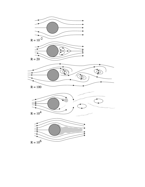
Figure 1: drawn following Feynman’s lectures [61]

First, recirculating eddies form behind the cylinder and detach themselves in a periodic way, giving rise to the Kármán street of alternating vortices. Thus, the first two symmetries are broken and a discrete $t$-invariance is all that is left over from the continuous $t$-invariance. Upon further increase of the order parameter $R$, the last invariance also breaks down. This represents a spontaneous breaking of symmetries, because the symmetries of the equations of motion and boundary conditions are not present in the observed solution for large Reynolds number.

Interestingly enough, in the present example, all symmetries are again restored in a statistical sense (and far from the boundaries) for very large values of $R$ : in fact, a homogeneous isotropic turbulence is observed in this case. It should be noted that complete symmetry in statistical physics means a completely irregular distribution when space- or time averages are considered. (There are no spatial correlations in the distribution - see [60] for more precise definitions.)

6.2 Miscellaneous and some important asymmetries

We conclude with some remarks on the breaking of the basic geometric symmetries in physical systems. Lorentz invariance is broken in finite temperature field theory since the heat bath defines a privileged reference frame [62] - see the lectures of C. Lucchesi. Some of the discrete symmetries ($P,C$ and $T$) or combinations thereof are violated in the microscopic world [63]. Actually, some of them are also broken at the macroscopic level, in particular in thermodynamics : while the basic equations of classical or quantum mechanics governing the dynamics of particles are invariant under the operation of time reversal (i.e. describe reversible processes), the processes observed at the macroscopic level, like the conduction of heat, do not have this property and are irreversible [64]. A further example is provided by cosmology, i.e. the study of the evolution of the universe. Note that the latter does not represent a physical system like any other since it is unique ; it is believed to have had a definite time of beginning and it is expanding. Therefore, cosmological time will not look the same if delayed in time, i.e. things are not invariant under translations in time. All these puzzles related to the arrow of time have intrigued scientists since Boltzmann’s pioneering work on statistical mechanics and they have stimulated intensive research [65].

Mention should also be made of two other asymmetries to whose understanding a lot of endeavor and work has been devoted in recent years. These are the baryon asymmetry in the universe (i.e. the question why matter is much more abundant in our universe than antimatter) [66] and the origin of chiral asymmetry in living systems (i.e. the fact that some of the basic organic structures only occur with one chirality in nature) [67].

7 Conclusion

The reader may find it disappointing or unsatisfactory to close our excursion on symmetries with asymmetries. However, symmetries and asymmetries often coexist in nature just as bad and good moments are parts of our daily life : they all have their right of being and without the hard times you would probably not appreciate the better ones to the right extent.

Acknowledgments

I wish to thank C. Doyen, S. Gourmelen, M. Kibler, C. Lucchesi and S. Theisen for pleasant discussions and useful remarks on the symmetries of nature. I also express my gratitude to Z. Hernaus for his skillful production of the graphics.

Appendix A Appendix

Further details concerning the notions summarized in this appendix are to be found in references [3].

A.1 On (Lie) groups and algebras

Definition 3

A group $(G,\circ)$ consists of a set $G$ together with a composition law denoted by $\circ$ which associates an element $x\circ y\in G$ to each pair of elements $(x,y)\in G\times G$ such that the following properties are satisfied :

1. Associativity : $\ x\circ(y\circ z)=(x\circ y)\circ z\;$ for all $\;x,y,z\in G$.

2. There exists a neutral element (identity), i.e. an element $e\in G$ which is such that $\ e\circ x=x\circ e=x\$ for all $x\in G$.

3. For each $x\in G$, there exists an inverse, i.e. an element $x^{-1}\in G$ such that $x\circ x^{-1}=x^{-1}\circ x=e$.

The group is said to be abelian if the commutative law $x\circ y=y\circ x$ holds for all $x,y\in G$.

If the elements of $G$ only satisfy the first two properties, then $(G,\circ)$ is called a semigroup.

If the group operation is ‘multiplicative’ (e.g. multiplication of real numbers), then the identity is denoted by $1$. If the operation is ‘additive’ (e.g. addition of real numbers), the identity is denoted by $0$ and the inverse $x^{-1}$ by $-x$.

Examples of (abelian) groups are given by $({\bf R},+)$, $({\bf Z},+)$ and $({\bf R}-\{0\},\cdot)$, $({\bf R}_{+},\cdot)$ where ${\bf R}_{+}$ denotes the set of positive real numbers which may be identified with $\{{\rm e}^{a}\,|\,a\in{\bf R}\}$. On the other hand, $({\bf Z}-\{0\},\cdot)$ is only a semigroup, because the inverse $1/n$ of an integer $n$ is not an integer (except for $n=\pm 1$).

Some particularly interesting groups are the Lie groups, i.e. groups whose elements can be parametrized by one or several real numbers ; the number of these parameters is referred to as the dimension of the Lie group. For instance, $({\bf R}^{n},+)$ is an $n$-dimensional abelian Lie group and so is the group $({\cal T}_{n},\circ)$ of translations of ${\bf R}^{n}$ introduced in section 3.1 $({\cal T}_{n}=\{T_{a}\,|\,a\in{\bf R}^{n}\})$. $({\bf R}-\{0\},\cdot)$ and $({\bf R}_{+},\cdot)$ are $1$-dimensional (hence abelian) Lie groups.

An important example of a non-abelian Lie group is given by the special orthogonal group $SO(3)$, i.e. the group of rotations around the origin of ${\bf R}^{3}$,

$$SO(3)=\{3\times 3\;\mbox{matrices}\ A\ \mbox{with real coefficients}\ |\;A^{t}A={\bf 1}_{3},\,{\rm det}\,A=1\}\ \ ,$$

the group operation being the multiplication of matrices. This group contains in particular the rotation $R_{3}(\varphi)$ by an angle $\varphi\in{\bf R}$ around the $z$-axis,

$$\left[\begin{array}[]{c}x^{\prime}\\ y^{\prime}\\ z^{\prime}\end{array}\right]=\left[\begin{array}[]{ccc}\cos\varphi&-\sin\varphi&0\\ \sin\varphi&\cos\varphi&0\\ 0&0&1\end{array}\right]\left[\begin{array}[]{c}x\\ y\\ z\end{array}\right]\equiv R_{3}(\varphi)\left[\begin{array}[]{c}x\\ y\\ z\end{array}\right]$$

as well as the analogous rotations around the $x$- and $y$-axis :

$$R_{1}(\varphi)=\left[\begin{array}[]{ccc}1&0&0\\ 0&\cos\varphi&-\sin\varphi\\ 0&\sin\varphi&\cos\varphi\\ \end{array}\right]\quad,\quad R_{2}(\varphi)=\left[\begin{array}[]{ccc}\cos\,\varphi&0&\sin\,\varphi\\ 0&1&0\\ -\sin\,\varphi&0&\cos\,\varphi\\ \end{array}\right]\ \ .$$

A rotation by an angle $\varphi$ around an arbitrary direction in space can be characterized by a vector $(\alpha,\beta,\gamma)\in{\bf R}^{3}$ pointing in this direction and having a length equal to $\varphi$. Thus, any element of $SO(3)$ is labeled by three real parameters : this Lie group is three-dimensional and it is non-abelian, because rotations do not commute in general. Another example of a matrix Lie group is given by the special unitary group $SU(n)$ defined in section 3.3. These matrix groups and ${\cal T}_{n}$ all represent examples of Lie transformation groups, i.e. groups whose elements act on a certain space.

To every Lie group one can associate its Lie algebra. If the former consists of transformations on a certain space, the latter represents the set of infinitesimal transformations on this space. For concreteness, we consider the rotation $R_{3}(\varphi)$ by an angle $\varphi$ which is close to $0$ (i.e. $R_{3}(\varphi)$ is close to the identity rotation) and expand it in a Taylor series around $\varphi=0$ :

$$R_{3}(\varphi) = R_{3}(0)+\left.\displaystyle{dR_{3}\over d\varphi}\right|_{\varphi=0}\ \varphi\,+\,...$$

$$= {\bf 1}_{3}+r_{3}\;\varphi+...\ \ .$$

By this way of reasoning, one finds that the rotations $R_{1}(\varphi),R_{2}(\varphi),R_{3}(\varphi)$ admit as ‘infinitesimal generators’ the antisymmetric matrices

$$r_{1}=\left[\begin{array}[]{ccc}0&0&0\\ 0&0&-1\\ 0&1&0\end{array}\right]\quad,\quad r_{2}=\left[\begin{array}[]{ccc}0&0&1\\ 0&0&0\\ -1&0&0\end{array}\right]\quad,\quad r_{3}=\left[\begin{array}[]{ccc}0&-1&0\\ 1&0&0\\ 0&0&0\end{array}\right]\ \ .$$ (A.2)

In terms of the Lie commutator (of matrices)

$$\framebox{\mbox{$\ {[A,B]}\equiv AB-BA\ $}}\ \ ,$$ (A.3)

we have

$$\left.\begin{array}[]{l}{[r_{1},r_{2}]}=r_{3}\\ {[r_{3},r_{1}]}=r_{2}\\ {[r_{2},r_{3}]}=r_{1}\end{array}\right\}\ \Longleftrightarrow\ \framebox{\mbox{$\ [r_{j},r_{k}]=\sum_{l=1}^{3}\varepsilon_{jkl}\,r_{l}\ $}}\ \ {\rm for}\ \;j,k\in\{1,2,3\}\ \ .$$ (A.4)

Here, the so-called structure constants $\varepsilon_{jkl}$ are the elements of the totally antisymmetric tensor of rank three normalized by $\varepsilon_{123}=1$ (i.e. $1=\varepsilon_{123}=\varepsilon_{312}=\varepsilon_{231}=-\varepsilon_{213}=-\varepsilon_{132}=-\varepsilon_{321}$ and $\varepsilon_{jkl}=0$ otherwise).

By definition, the Lie algebra $so(3)$ associated to the Lie group $SO(3)$ (which is $3$-dimensional) is the real, $3$-dimensional vector space consisting of all linear combinations of the matrices $r_{1},r_{2}$ and $r_{3}$ together with the Lie bracket operation defined by (A.3). Explicitly, we have

$$so(3)=\{3\times 3\;\mbox{matrices}\ A\ \mbox{with real coefficients}\ |\;A^{t}=-A\}\ \ .$$

Note that two Lie groups which “look the same in the neighborhood of the identity” admit the same Lie algebra since the latter is only defined by considering such a neighborhood. E.g. the elements of ${\bf R}-\{0\}$ and ${\bf R}_{+}$ which are close to the identity $1$ have the form ${\rm e}^{a}=1+1\cdot a+...$ with $a\in{\bf R}$ and therefore both Lie groups admit ${\bf R}$ as their Lie algebra.

Lie algebras may also be introduced without any reference to Lie groups : a (real) abstract Lie algebra is a (real) vector space ${\cal G}$ together with an operation $[\,,\,]:{\cal G}\times{\cal G}\to{\cal G}$ which is (${\bf R}$-) bilinear, antisymmetric and satisfies the Jacobi identity (i.e. $0=[A,[B,C]]\,+$ cyclic permutations of $A,B,C$ ). E.g. the vector space ${\bf R}^{3}$ together with the cross product as commutator, $[\vec{a},\vec{b}\,]=\vec{a}\times\vec{b}$, represents an abstract Lie algebra. Note that the vectors $\vec{e}_{1}=(1,0,0),\vec{e}_{2}=(0,1,0),\vec{e}_{3}=(0,0,1)$ which define the canonical basis of ${\bf R}^{3}$ satisfy $\vec{e}_{j}\times\vec{e}_{k}=\sum_{l=1}^{3}\varepsilon_{jkl}\,\vec{e}_{l}$ for $j,k\in\{1,2,3\}$, i.e. the same relation as the matrices $r_{j}\in so(3)$.

While we passed from the Lie group $SO(3)$ to the associated Lie algebra $so(3)$ by differentiation, we can go the other way round by exponentiation : in fact, one can verify that $R_{3}(\varphi)={\rm exp}\,(\varphi r_{3})={\bf 1}_{3}+\varphi r_{3}+...$ where the exponential of matrices is defined by the Taylor series expansion (${\rm exp}\,A\equiv\sum_{n=0}^{\infty}{1\over n!}A^{n}$).

To summarize, the sets of finite and infinitesimal transformations are related as follows :

$$\ \begin{array}[]{l c c c r}&&{\rm differentiate}&&\\ {\rm Lie\ group}&&\rightleftharpoons&&{\rm Lie\ algebra}\\ &&{\rm exponentiate}&&\end{array}\$$

Note that, in general, the exponentiation of Lie algebra elements does not allow to recover all Lie group elements. E.g. exponentiation of the Lie algebra ${\bf R}$ associated to the Lie group $({\bf R}-\{0\},\cdot)$ yields the Lie group $\{{\rm e}^{a}\,|\,a\in{\bf R}\}={\bf R}_{+}$, i.e. the component of ${\bf R}-\{0\}$ which is connected to the identity $1$.

Before proceeding further, we recall that a homomorphism between two sets which are supplemented with additional structures is a structure preserving map. Thus, a homomorphism of groups is a map between two groups which preserves the group multiplication. E.g. the groups $({\bf R}^{n},+)$ and $({\cal T}_{n},\circ)$ can be related by the map

$$f\ :\ \ {\bf R}^{n} \!\longrightarrow\ \;{\cal T}_{n}$$

$$a \!\longmapsto\ \;T_{a}\ \ ,$$

which is a homomorphism, because $f(a+b)=T_{a+b}=T_{a}\circ T_{b}=f(a)\circ f(b)$. The groups $({\bf R},+)$ and $({\bf R}_{+},\cdot)$ may be related by the homomorphism $a\mapsto{\rm e}^{a}$.

Analogously, a homomorphism of Lie algebras is a map which preserves the Lie algebra structure, i.e. a linear map preserving the Lie bracket. For instance, the Lie algebra ${\bf R}^{3}$ (with the cross product as commutator) and the matrix Lie algebra $so(3)$ can be related by the following mapping of the basis vectors,

$$f\ :\ \ {\bf R}^{3} \!\longrightarrow\ \;so(3)$$

$$\vec{e}_{j} \!\longmapsto\ \;r_{j}\ \ ,$$

which we extend in a linear way to all linear combinations of vectors : this map is a homomorphism since it is linear (by definition) and

$$[f(\vec{e}_{j}),f(\vec{e}_{k})]=[r_{j},r_{k}]=\sum_{l=1}^{3}\varepsilon_{jkl}\,r_{l}=\sum_{l=1}^{3}\varepsilon_{jkl}\,f(\vec{e}_{l})=f(\sum_{l=1}^{3}\varepsilon_{jkl}\,\vec{e}_{l})=f(\vec{e}_{j}\times\vec{e}_{k}),$$

which implies $[f(\vec{a}),f(\vec{b})]=f(\vec{a}\times\vec{b})$ for all $\vec{a},\vec{b}\in{\bf R}^{3}$ by linearity.

Actually, all of these illustrations represent examples of isomorphisms, i.e. bijective maps such that the map and its inverse are homomorphisms. Two groups, Lie algebras,… related by an isomorphism have exactly the same structure and thus may be identified with each other for many purposes.

A.2 About representations

A.2.1 Representation of a (Lie) group

Suppose you want to let the elements of the group $SU(2)$, i.e. complex $2\times 2$ matrices act linearly on vectors of ${\bf R}^{3}$ in such a way that the group operation is preserved. More generally, you may want to define the action of a group $G$ on a real vector space $V$ of finite dimension $n$. The device which allows to realize this idea is provided by the next definition.

Let $GL(V)$ denote the group of all invertible linear maps from $V$ to itself, the group operation being the composition of maps. This group is isomorphic to the group $GL(n,{\bf R})$ of all invertible $n\times n$ matrices with real coefficients, the group law being the matrix multiplication.

Definition 4

A representation $D$ of the group $G$ on the vector space $V$ is a homomorphism from the group $G$ to the group $GL(V)$, i.e. it is a map

$$D\ :\ \ G \!\longrightarrow\ \;GL(V)$$ (A.5)

$$g \!\longmapsto\ \;D(g)$$

such that the linear operators $D(g)$ satisfy

$$\framebox{\mbox{$\ D(g_{1}\circ g_{2})=D(g_{1})\circ D(g_{2})\ $}}\quad for\ \,all\ g_{1},g_{2}\in G\ \ .$$ (A.6)

The dimension of the representation is the dimension of the representation space, i.e. ${\rm dim}\,D={\rm dim}\,V$.

We now come back to the question concerning the action of $SU(2)$ on ${\bf R}^{3}$ : rather than providing a complete answer (which may be found in many textbooks on quantum mechanics or quantum field theory), we give an illustration for a particular element of $SU(2)$ :

$$D\ :\ SU(2) \longrightarrow\ \ SO(3)\subset GL(3,{\bf R})$$

$$A_{\varphi}\equiv\left[\begin{array}[]{cc}{\rm e}^{{\rm i}\varphi/2}&0\\ 0&{\rm e}^{-{\rm i}\varphi/2}\end{array}\right] \longmapsto\ \ D(A_{\varphi})=\left[\begin{array}[]{ccc}\cos\varphi&-\sin\varphi&0\\ \sin\varphi&\cos\varphi&0\\ 0&0&1\end{array}\right]\ \ .$$ (A.12)

Here, $\varphi$ is a real parameter and it is straightforward to verify that the group product is preserved by the mapping $D$, i.e. $D(A_{\varphi_{1}}A_{\varphi_{2}})=D(A_{\varphi_{1}})D(A_{\varphi_{2}})$.

The previous definition can be generalized to the cases where $V$ is a complex vector space or where its dimension is not finite. In the latter case, one encounters the technical complication that the linear operators acting on $V$ can, in general, only be defined on a subspace of $V$ (e.g. the action of differential operators on function spaces can only be defined on sufficiently smooth functions). However, in physics one usually deals with vector spaces that are supplemented with a Hilbert space structure, e.g. the (complex, infinite-dimensional) Hilbert space of square-integrable functions on ${\bf R}$,

$${\cal H}\equiv{\cal L}^{2}({\bf R})=\{\psi:{\bf R}\to{\bf C}\ |\;\int_{-\infty}^{+\infty}|\psi(x)|^{2}dx<\infty\}$$ (A.13)

describing the quantum mechanical states of a particle moving on the real axis. In this case, one generally considers unitary representations, i.e. the group representative $D(g)$ of each element $g\in G$ is a unitary operator on the Hilbert space ${\cal H}$ (and thereby defined on all vectors of ${\cal H}$).

Let us illustrate this notion by an example involving the space (A.13). Suppose you want to translate the wave function $\psi\in{\cal H}$ of a particle moving on the real axis by an amount $a\in{\bf R}$. In other words, you want to consider the action of the translation $T_{a}\in{\cal T}_{1}$ on the vector $\psi$ : the group element $T_{a}$ acts by means of the Hilbert space operator

$$D(T_{a})\ :\ \ {\cal H} \!\stackrel{{\scriptstyle{\rm linear}}}{{\longrightarrow}}\ \;{\cal H}$$

$$\psi \!\longmapsto\ \;D(T_{a})\psi\equiv\psi_{a}$$

defined by

$$\psi_{a}(x):=\psi(x-a)\ \ .$$ (A.14)

The operator $D(T_{a})$ is unitary and it defines a representation since

$$D(T_{a}\circ T_{b})\,\psi=D(T_{a+b})\,\psi=\psi_{a+b}=D(T_{a})\,\psi_{b}=D(T_{a})D(T_{b})\,\psi\ \ {\rm for}\ {\rm all}\ \ \psi\in{\cal H}\,,$$

henceforth $D(T_{a}\circ T_{b})=D(T_{a})D(T_{b})$. The dimension of this unitary representation of the translation group ${\cal T}_{1}$ is infinite.

A.2.2 Representation of a Lie algebra

As in the previous section, we consider a real vector space $V$ of finite dimension. The set $gl(V)$ consisting of all linear operators from $V$ to itself, equipped with the usual linear operations (addition of operators and multiplication of operators by real numbers) and with the commutator $[A,B]=A\circ B-B\circ A$ is a real Lie algebra : it is the Lie algebra associated to the Lie group $GL(V)$.

Definition 5

A representation $d$ of the (real) Lie algebra ${\cal G}$ on the vector space $V$ is a homomorphism from the Lie algebra ${\cal G}$ to the Lie algebra $gl(V)$, i.e. it is a map

$$d\ :\ \ {\cal G} \!\longrightarrow\ \;gl(V)$$ (A.15)

$$t \!\longmapsto\ \;d(t)$$

such that the linear operators $d(t)$ satisfy

$$\framebox{\mbox{$\ d(c_{1}t_{1}+c_{2}t_{2})=c_{1}d(t_{1})+c_{2}d(t_{2})\ $}}\quad and\quad\framebox{\mbox{$\ d([t_{1},t_{2}])=[d(t_{1}),d(t_{2})]\ $}}$$ (A.16)

for all $t_{1},t_{2}\in{\cal G}$ and $c_{1},c_{2}\in{\bf R}$. Furthermore, one defines ${\rm dim}\,d={\rm dim}\,V$ .

As an illustration, we consider the operators $L_{1},L_{2},L_{3}$ of angular momentum which act on the Hilbert space ${\cal H}={\cal L}^{2}({\bf R}^{3})$ of quantum mechanics : they admit a common invariant domain ${\cal D}$ which is dense in ${\cal H}$ and on which they satisfy the algebra

$$[L_{j},L_{k}]={\rm i}\hbar\,\sum_{l=1}^{3}\varepsilon_{jkl}\,L_{l}\qquad\quad{\rm for}\ \;j,k\in\{1,2,3\}\ \ .$$

Therefore, the mapping

$$d\ :\ so(3) \longrightarrow\ gl({\cal D})$$ (A.17)

$$r_{k} \longmapsto\ d(r_{k})\equiv{1\over{\rm i}\hbar}\,L_{k}$$

(extended by linearity to all elements of the vector space $so(3)$) is a representation of the Lie algebra of infinitesimal rotations on the Hilbert space ${\cal H}$. (We leave the verification of the properties (A.16) as an exercise.)

The image $D(G)$ of a Lie group $G$ under a representation $D$ is again a Lie group and similarly $d({\cal G})$ is a Lie algebra. The passage from the set $D(G)$ of finite transformations to the set $d({\cal G})$ of infinitesimal transformations can be performed in the same way as the one between $G$ and ${\cal G}$, i.e. by differentiation and exponentiation, respectively.

References

- [1] H. Weyl, “Symmetry”, Princeton University Press 1952 ;
- [2] D’Arcy W. Thompson, “On Growth and Form”, Cambridge 1917 ;
- [3] R. Gilmore, “Lie Groups, Lie Algebras, and some of their Applications”, Wiley 1974 ; B.G. Wybourne, “Classical Groups for Physicists”, Wiley 1974 ; D.H. Sattinger and O.L. Weaver, “Lie Groups and Algebras with Applications to Physics, Geometry, and Mechanics”, Applied Mathematical Sciences Vol. 61 , Springer 1986 ; W. Ludwig and C. Falter, “Symmetries in Physics - Group theory applied to physical problems”, Springer Series in Solid-State Sciences Vol. 64, Springer 1988 ; J.F. Cornwell, “Group Theory in Physics”, Vol. I - III, Academic 1984, 1989 ; G.G.A. Baeuerle and E.A. de Kerf, “Lie Algebras part 1 : finite and infinite dimensional Lie algebras and applications to physics”, North-Holland 1990; S. Sternberg, “Group Theory and Physics”, Cambridge University Press 1994 ;
- [4] R. P. Feynman, “The Character of Physical Law”, Penguin Books 1965 ;
- [5] L. Tarassow, “Symmetrie, Symmetrie! - Strukturprinzipien in Natur und Technik”, Spektrum Akademischer Verlag 1993 ;
- [6] H. Genz und R. Decker, “Symmetrie und Symmetriebrechung in der Physik”, Vieweg 1991 ;
- [7] J. Sivardière, “La symétrie en mathématiques, physique et chimie”, Presses Universitaires de Grenoble 1995 ;
- [8] M. Eigen und R. Winkler, “Das Spiel - Naturgesetze steuern den Zufall”, Piper 1975;
- [9] T. Mayer-Kuckuk, “Der gebrochene Spiegel - Symmetrie, Symmetriebrechung und Ordnung in der Natur”, Birkhäuser 1989 ;
- [10] J.-P. Blaizot et J.-C. Tolénado, “Symétries et physique microscopique”, Ellipses 1997 ;
- [11] “Symétries et Physique Nucléaire”, Ecole Joliot-Curie de Physique Nucléaire (IN2P3) 1986 ;
- [12] P. Chossat, “Les symétries brisées”, Pour la Science 1996 ;
- [13] L. Fonda and G.C. Ghirardi, “Symmetry Principles in Quantum Physics”, Marcel Dekker 1970 ; J.McL. Emmerson, “Symmetry Principles in Particle Physics”, Oxford University Press 1972 ; J. Leite Lopes, “Lectures on Symmetries”, Gordon and Breach 1969 ;
- [14] C.D. Froggatt and H.B. Nielsen, “Origin of Symmetries”, World Scientific 1991 ; J. Rosen (ed.), “Symmetry in Physics : Selected Reprints”, American Association of Physics Teachers 1982 ; “Symmetry in Nature - A volume in honor of Luigi A. Radicati di Brozolo”, Scuola Normale Superiore Pisa 1989 ;
- [15] J. Rosen, “Symmetry in Science - An introduction to the general theory”, Springer 1995 ;
- [16] E. Wigner, “Symmetries and Reflections”, Indiana University Press 1967 ; R.G. Newton, “What makes the nature tick?”, Harvard University Press 1993;
- [17] M. Schottenloher, “Geometrie und Symmetrie in der Physik - Leitmotiv der Mathematischen Physik”, Vieweg 1995 ;
- [18] A.V. Shubnikov and V.A. Koptsik, “Symmetry in Science and Art”, Plenum Press 1974 ; M. Field and M. Golubitsky, “Symmetry in Chaos - a search for pattern in mathematics, art and nature”, Oxford University Press 1992 ;
- [19] M.C. Escher, “Graphik und Zeichnungen”, Benedikt Taschen 1993 ; B. Ernst, “Der Zauberspiegel des M.C. Escher”, Benedikt Taschen 1994;
- [20] J. Fröhlich et al. (eds.), “New Symmetry Principles in Quantum Field Theory”, Plenum Press 1992 ;
- [21] B. Grünbaum and G.C. Shepard, “Tilings and Patterns - An introduction”, Freeman 1989 ;
- [22] J.H. Conway and R.K. Guy, “The Book of Numbers”, Springer 1996 ;
- [23] J. Bronowski, “Der Aufstieg des Menschen - Stationen unserer Entwicklungsgeschichte”, Ullstein 1973 ;
- [24] C. Giacovazzo et al., “Fundamentals of Crystallography”, Oxford University Press 1992 ; M. Senechal, “Quasicrystals and Geometry”, Cambridge University Press 1995 ;
- [25] H. Knörrer, “Geometrie”, Vieweg 1996 ;
- [26] J. Honerkamp and H. Römer, “Theoretical Physics - a classical approach”, Springer 1993 ;
- [27] R.G. Sachs, “The Physics of Time Reversal”, University of Chicago Press 1987 ;
- [28] S. Weinberg, “The Quantum Theory of Fields”, Vol. I and II, Cambridge University Press 1995 and 1996 ;
- [29] B.A. Dubrovin, A.T. Fomenko and S.P. Novikov, “Modern Geometry - Methods and Applications”, Part I , Springer 1984 ;
- [30] S.B. Treiman, R. Jackiw and D.J. Gross, “Lectures on Current Algebra and its Applications”, Princeton University Press 1972 ; S. Coleman, “Aspects of Symmetry - Selected Erice Lectures”, Cambridge University Press 1985 ;
- [31] G.L. Sewell, “Quantum Theory of Collective Phenomena”, Oxford University Press 1986 ; L.E. Reichl, “A Modern Course in Statistical Mechanics”, University of Texas Press 1980 ;
- [32] P. DiFrancesco, P. Mathieu and D. Senechal, “Conformal Field Theory”, Springer 1997 ;
- [33] M.B. Green, J.H. Schwarz and E. Witten, “Superstring Theory”, Vol. 1 and 2, Cambridge University Press 1987 ; D. Lüst and S. Theisen, “Lectures on String Theory”, Lecture Notes in Physics Vol. 346, Springer 1989 ;
- [34] L. Corwin, Y. Ne’eman and S. Sternberg, “Graded Lie algebras in mathematics and physics (Bose-Fermi symmetry)”, Rev.Mod.Phys. 47 (1975) 573 ; B. DeWitt, “Supermanifolds”, second edition, Cambridge University Press 1992 ; V.A. Kostelecký and D.K. Campbell, eds., “Supersymmetry in Physics”, North Holland 1985 ;
- [35] M.F. Sohnius, “Introducing supersymmetry”, Phys.Rep. 128 (1985) 39 ; I.L. Buchbinder and S.M. Kuzenko, “Ideas and methods of supersymmetry and supergravity or a walk through superspace”, IOP 1995 ;
- [36] G. Junker, “Supersymmetric Methods in Quantum and Statistical Physics”, Texts and Monographs in Physics, Springer 1996 ; H. Kalka und G. Soff, “Supersymmetrie”, Teubner 1997 ;
- [37] H.E. Haber and G.L. Kane, “The search for supersymmetry : probing physics beyond the standard model”, Phys.Rep. 117 (1985) 75 ;
- [38] T.-P. Cheng and L.-F. Li, “Gauge Theory of Elementary Particle Physics”, Oxford University Press 1984 ;
- [39] L.H. Ryder, “Quantum Field Theory”, Cambridge University Press 1985 ;
- [40] N. Straumann, “General Relativity and Relativistic Astrophysics”, Springer 1984 ;
- [41] R.U. Sexl und H.K. Urbantke, “Gravitation und Kosmologie”, Bibliographisches Institut 1987 ;
- [42] V.G. Makhankov, Y.P. Rybakov and V.I. Sanyuk, “The Skyrme Model - Fundamentals, Methods, Applications”, Springer 1993 ;
- [43] J. Louis und S. Theisen, “Dualität in Feld- und Stringtheorien”, Phys.Bl. Dez. 1997 ; D.I. Olive, “Introduction to Electromagnetic Duality”, Nucl.Phys.B (Proc. Suppl.) 58 (1997) 43 ; A. Bilal, “Duality in SUSY Yang-Mills Theory: A pedagogical introduction to the work of Seiberg and Witten”, hep-th/9601007;
- [44] M. Schroeder, “Fractals, Chaos, Power Laws - Minutes from an infinite paradise”, Freeman 1991 ;
- [45] P. Collet and J.-P. Eckmann, “Iterated Maps on the Interval as Dynamical Systems”, Birkhäuser 1980 ; S.H. Strogatz, “Nonlinear Dynamics and Chaos - With applications to physics, biology, chemistry and engineering”, Addison-Wesley 1994 ;
- [46] J. de Boer, F. Harmsze and T. Tjin, “Non-linear finite -symmetries and applications in elementary systems”, Phys.Rep. 272 (1996) 139 ;
- [47] P. Bouwknegt and K. Schoutens, “ -symmetry in conformal field theory”, Phys.Rep. 223 (1993) 183 ;
- [48] V. Chari and A. Pressley, “A guide to Quantum Groups”, Cambridge University Press 1994 ; C. Kassel, “Quantum Groups”, Graduate Texts in Mathematics Vol.155, Springer 1995 ;
- [49] P. Goddard and D. Olive, “Kac-Moody and Virasoro algebras in relation to quantum physics”, Int.J.Mod.Phys. A1 (1986) 303 ;
- [50] F. Gieres, “Geometry of Supersymmetric Gauge Theories - Including an introduction to BRS differential algebras and anomalies”, Lecture Notes in Physics Vol. 302, Springer 1988 ;
- [51] R.A. Bertlmann, “Anomalies in Quantum Field Theory”, Oxford University Press 1996 ;
- [52] O. Piguet and S.P. Sorella, “Algebraic Renormalization - Perturbative renormalization, symmetries and anomalies”, Lecture Notes in Physics - Monographs m 28, Springer 1995 ;
- [53] N.J. Vilenkin and A.U. Klimyk, “Representations of Lie Groups and Special Functions”, Vol. 1-3, Kluwer 1991, 1993, 1992 ;
- [54] W. Miller Jr., “Symmetry and Separation of Variables”, Addison-Wesley 1977 ;
- [55] H. Stephani, “Differential Equations - Their solution using symmetries”, Cambridge University Press 1989 ; P.J. Olver, “Applications of Lie Groups to Differential Equations”, Graduate Texts in Mathematics Vol. 107 , Springer 1986 ;
- [56] B.G. Adams, “Algebraic Approach to Simple Quantum Systems”, Springer 1994 ;
- [57] F. Iachello, “Lie algebras and exactly solvable problems in quantum mechanics”, in “Strings and Symmetries”, G. Aktaş et al. (eds.), Lecture Notes in Physics Vol. 447, Springer 1995 ;
- [58] D. Kramer, H. Stephani, M. McCallum and E. Herlt, “Exact Solutions of Einstein’s Field Equations”, DVW, Berlin 1980 ;
- [59] J. Lopuszánski, “An Introduction to Symmetry and Supersymmetry in Quantum Field Theory”, World Scientific 1991 ; H. Reeh, “Symmetries, currents and infinitesimal generators“, in “Statistical Mechanics and Field Theory”, R.N. Sen and C. Weil, eds., Halsted/Wiley 1972; A.H. Völkel, “Fields, Particles and Currents”, Lecture Notes in Physics Vol. 66, Springer 1977 ;
- [60] U. Frisch, “Turbulence - The legacy of A.N. Kolmogorov”, Cambridge University Press 1995 ;
- [61] R.P. Feynman, R.B. Leighton and M. Sands, “The Feynman Lectures on Physics”, Vol. 2, Addison-Wesley 1964 ;
- [62] M. le Bellac, “Thermal Field Theory”, Cambridge University Press 1996 ;
- [63] C. Jarlskog (ed.), “CP violation”, World Scientific 1989 ;
- [64] R. Balian, “From Microphysics to Macrophysics - Methods and applications of Statistical Physics, Vol. I”, Texts and Monographs in Physics, Springer 1991 ;
- [65] P.C.W. Davies, “The Physics of Time Asymmetry”, Surrey University Press, 1974 ; J.J. Halliwell, J. Pérez-Mercader and W.H. Zurek (eds.), “Physical Origins of Time Asymmetry”, Cambridge University Press, 1994 ; S. Savitt (ed.), “Time’s Arrows Today”, Cambridge University Press, 1994; E. Klein et M. Spiro (eds.), “Le temps et sa flèche”, Frontières 1994 ; A. Magnon, “Arrow of Time and Reality : in search of a conciliation”, World Scientific 1997 ;
- [66] E.W. Kolb and M.S. Turner, “The Early Universe”, Addison-Wesley, 1990;
- [67] D.B. Cline (ed.), “Physical Origin of Homochirality in Life”, Oxford University Press, 1997 ;
- [68] T. Bröcker and T. tom Dieck, “Representations of Compact Lie Groups”, Graduate Texts in Mathematics Vol.98 , Springer 1985 ;
- [69] A.O. Barut and R. Raczka, “Theory of Group Representations and Applications”, Polish Scientific Publishers 1977 .