Analytic structure of scalar composites in the symmetric phase of the gauged Nambu–Jona-Lasinio model

Abstract

The gauged Nambu–Jona-Lasinio model in the quenched-ladder approximation has nontrivial dynamics near a critical scaling region (critical curve) separating a chiral symmetric and a dynamically chiral symmetry broken phase. Scalar and pseudoscalar composites corresponding to the four-fermion and gauge interactions become relevant degrees of freedom at long distances, which is reflected in the appearance of a large anomalous dimension of the four-fermion operators. A method is introduced for solving the Schwinger-Dyson equation for the Yukawa vertex in specific kinematic regimes. This allows one to derive an analytic expression for the scalar propagator, which is valid along the entire critical curve. The mass and width of the scalar composites in the critical scaling region are reexamined and the conformal phase transition at gauge coupling $\alpha_{0}=\alpha_{c}$ is discussed.

I Introduction

The recent interest in the gauged Nambu–Jona-Lasinio (GNJL) model has been stimulated by its importance for constructing extended technicolor models (ETC) and the top-quark condensate model (for an introduction see Ref. [1]).

It is well known that in the quenched-ladder approximation the GNJL model has a nontrivial phase structure [2] in the coupling constant plane $(g_{0},\alpha_{0})$, where $g_{0}\equiv G_{0}\Lambda^{2}/4\pi^{2},\alpha_{0}\equiv e_{0}^{2}/4\pi$ as shown in Fig. 1 ($\Lambda$ is a cutoff). The critical line is

$$g_{c}(\alpha_{0})\equiv\frac{1}{4}\left(1+\sqrt{1-\frac{\alpha_{0}}{\alpha_{c}}}\right)^{2},\qquad 0\leq\alpha_{0}<\alpha_{c}=\frac{\pi}{3}$$ (1)

at $g_{0}>{1\over 4}$, and

$$\alpha_{0}=\alpha_{c}$$ (2)

at $g_{0}\leq{1\over 4}$, above which the gap equation for the fermion self-energy $\Sigma(p)$ has a nontrivial solution. Thus the chiral symmetry is dynamically broken, which implies the existence of a nonzero vacuum condensate $\langle\bar{\psi}\psi\rangle$. One end point $(g_{0}=1,\alpha_{0}=0)$ of the critical line corresponds to the ordinary NJL model, while the other one $(g_{0}=0,\alpha_{0}=\alpha_{c}=\pi/3)$ corresponds to pure QED. The interesting feature of the GNJL model is the observation that naively irrelevant chiral invariant four-fermion operators become relevant near the chiral phase transition [3] due to the appearance of a large anomalous dimension $\gamma_{m}$ of the operator $\bar{\psi}\psi$ along the critical curve Eq. (1), $2\geq\gamma_{m}\geq 1$, and $\gamma_{m}=1$ along the part of the critical line with $\alpha_{0}=\alpha_{c}$ [4]. Therefore the GNJL model is believed to be renormalizable as an interacting continuum theory near a critical scaling region (critical curve) in the coupling plane separating a chiral symmetric phase ($\chi S$) and a spontaneous chiral symmetry broken phase ($S\chi SB$).

In the ladder approximation it has been shown [5, 6, 7] that the GNJL model in four dimensions is indeed renormalizable, and that the anomalous dimension

$$\gamma_{m}\equiv-\Lambda\frac{\partial\ln m_{0}}{\partial\Lambda}$$ (3)

is

$$\gamma_{m} = 1-\omega+2\omega\frac{g_{0}}{g_{c}},\qquad g_{0}<g_{c}={1\over 4},\quad\omega=\sqrt{1-\alpha_{0}/\alpha_{c}},$$ (4)

$$\gamma_{m} = 1+\omega+2(g_{0}-g_{c}),\qquad g_{0}\geq g_{c}.$$ (5)

Fine-tuning the coupling $g_{0}$ to $g_{c}$ in $S\chi SB$ phase in such a way that $m_{d}/\Lambda\ll 1$, where $m_{d}\equiv\Sigma(0)$ is the dynamical mass of a fermion, a nontrivial continuum limit ($m_{d}/\Lambda\rightarrow 0$) can be reached just as in pure quenched QED [8, 9, 10]. The spectrum of such a theory contains pseudoscalar ($\pi$) and scalar ($\sigma$) bound states which become light and dynamically active in the vicinity of the critical line. Since the phase transition is second order along the part Eq. (1) of the critical curve, scalar and pseudoscalar resonances have been shown to be produced on the symmetric side of the curve, whose masses approach zero as the critical curve is approached [11]. The part of the critical curve, Eq. (2), with $\alpha_{0}=\alpha_{c}$ is rather special. For example, an abrupt change of the spectrum of light excitations occurs when the line $\alpha_{0}=\alpha_{c}$, $g_{0}<1/4$ is crossed: while light scalar and pseudoscalar excitations still persist in the broken phase, there are no such light excitations in the symmetric phase [6, 12]. A similar behavior has been revealed also in QED₃ [13]. This peculiar phase transition was referred to as a conformal phase transition (CPT) [14].

In this paper we study scalar composites ($\sigma$ and $\pi$ bosons) in the symmetric phase of the GNJL model. Computing the scalar propagator (see Fig. 2) requires knowledge of the full scalar-fermion-antifermion vertex ${\Gamma_{\rm S}}(p+q,p)$ which in turn satisfies the Bethe-Salpeter (BS) equation displayed in Fig. 3. We solve this BS equation in the ladder approximation (Fig. 4) but differ from the corresponding studies in Refs. [7, 11] who used an approximation for ${\Gamma_{\rm S}}(p+q,p)$ with zero boson momentum ($q=0$). A technique of expansion in the Chebyshev polynomials is introduced for solving the Yukawa vertex with nonzero boson momentum and consequently an explicit analytical expression is derived for the propagator of the $\sigma$ boson valid along the entire critical curve.

Our main physical conclusions are the same as in Refs. [6, 11, 12]: in the region $\alpha_{0}<\alpha_{c}$, $g_{0}>1/4$, in the symmetric phase, a spectrum of light resonances exists while at $\alpha_{0}<\alpha_{c},g_{0}<1/4$ there are no light resonances. Having obtained an analytical expression for the scalar propagator, we can analytically continue it into the region $\alpha_{0}>\alpha_{c}$ and find light tachyons there, signaling the instability of the symmetric solution.

The plan of the present paper is as follows. After introducing the GNJL model (Sec. II) we solve the equation for the Yukawa vertex with nonzero boson momentum in Sec. III keeping only the zero order Chebyshev harmonics. In Sec. IV we obtain an analytical expression for the boson propagator valid along the entire critical line and analyze its behavior in different asymptotical regimes. Sec. V is devoted to comparing our results for the Yukawa vertex and boson propagator with the corresponding ones in Refs. [7, 11]. In Sec. VI we discuss the behavior of the scalar propagator near the critical line (1) in the symmetric phase and, in particular, the mass and the width of resonances. The analysis of the scalar composites near the critical line (2) is given in Sec. VII, where we show the absence of light excitations at $\alpha_{0}\leq\alpha_{c}$ while analytically continuing the symmetric phase propagator into the region $\alpha_{0}\geq\alpha_{c}$ leads to the appearance of tachyonic states. We discuss this behavior from the viewpoint of the CPT conception proposed recently in Ref. [14]. We present our summary in Sec. VIII and in Appendix A we give an analysis of the contribution of higher order Chebyshev harmonics into the Yukawa vertex equation and scalar vacuum polarization.

II The Gauged Nambu–Jona-Lasinio model

The gauged NJL model is described by the Lagrangian

$${\cal L}_{\rm GNJL}=-{1\over 4}F^{2}_{\mu\nu}+\bar{\psi}(i\gamma^{\mu}D_{\mu}-m_{0})\psi+{G_{0}\over 2}[(\bar{\psi}\psi)^{2}+(\bar{\psi}i\gamma_{5}\psi)^{2}],$$ (6)

where $D_{\mu}=\partial_{\mu}-ie_{0}A_{\mu}$ is a covariant derivative, $e_{0}$ the gauge coupling constant, and the last term is a chirally invariant four-fermion interaction with $G_{0}$ the corresponding Fermi coupling constant. Another way to refer to this model is that it is QED with an additional four-fermion interaction. In the absence of a fermion mass term $m_{0}$ which breaks the chiral symmetry explicitly, the Lagrangian (6) possesses a $U(1)$ gauge symmetry and a global $U_{L}(1)\times U_{R}(1)$ chiral symmetry. (It is not difficult to extend our results for $SU_{L}(N_{f})\times SU_{R}(N_{f})$ chiral symmetry with $N_{f}$ fermion flavors.)

Let us introduce the chiral fields $\sigma$ and $\pi$ rewriting the Lagrangian (6) in the form

$${\cal L}_{\rm GNJL}=-{1\over 4}F^{2}_{\mu\nu}+\bar{\psi}i\gamma^{\mu}D_{\mu}\psi-\bar{\psi}(\sigma+i\gamma_{5}\pi)\psi-{1\over 2G_{0}}(\sigma^{2}+\pi^{2})+\frac{m_{0}}{G_{0}}\sigma.$$ (7)

One can readily verify the equivalence of the Lagrangians (6) and (7) by just making use of the Euler-Lagrange equations. Further we study mainly the chiral symmetric case with $m_{0}=0$.

With this Lagrangian we define the generating functional of the GNJL model by

$$Z_{\rm GNJL}[J,\eta,\bar{\eta},J_{\sigma},J_{\pi}]=N\int{\rm d}\mu\left(A,\bar{\psi},\psi,\sigma,\pi\right)\,\exp\left\{iS_{J}\right\},$$ (8)

where the “measure” is defined as

$${\rm d}\mu\left(A,\bar{\psi},\psi,\sigma,\pi\right)\equiv{\cal D}A{\cal D}\psi{\cal D}\bar{\psi}{\cal D}\sigma{\cal D}\pi,$$ (9)

and where the source-dependent action $S_{J}$ is

$$S_{J}=S_{\rm GNJL}+J_{\mu}A^{\mu}+\bar{\eta}\psi+\bar{\psi}\eta+J_{\sigma}\sigma+J_{\pi}\pi+{\cal S}_{\Lambda}.$$ (10)

The last term ${\cal S}_{\Lambda}$ represents the ultraviolet regulating part of the action. The starting point to derive the Schwinger-Dyson equations (SDEs) is the following formal identity:

$$\int{\rm d}\mu\left(A,\bar{\psi},\psi,\sigma,\pi\right)\,\frac{\delta iS_{\rm J}}{\delta\phi(x)}\exp\left\{iS_{J}\right\}=0,\quad\mbox{where}\quad\phi=A,\psi,\bar{\psi},\sigma,\pi,$$ (11)

from which the SDE for the propagators and vertices in momentum space can be obtained. For our purpose it is convenient to recall the SDEs for the scalar propagator and scalar vertex. The SDE equation for the scalar propagator is given by

$$\Delta_{\rm S}^{-1}(p)=-\frac{1}{G_{0}}+\Pi_{\rm S}(p^{2}),$$ (12)

where the scalar vacuum polarization is

$$\Pi_{\rm S}(p^{2})=i\int_{\Lambda}\frac{{\rm d}^{4}k}{(2\pi)^{4}}\,{\rm Tr}\left[S(k+p){\Gamma_{\rm S}}(k+p,k)S(k)\right]$$ (13)

(see Fig. 2), $S(k)$ is the full fermion propagator, and ${\Gamma_{\rm S}}(k+p,k)$ is the scalar fermion-antifermion vertex. The absence of kinetic terms for the $\sigma$ and $\pi$ fields in the Lagrangian is reflected in the constant bare propagator $-G_{0}$.

The scalar propagator is defined as the Fourier transform of the connected part of the correlator

$$\langle 0|T\left(\sigma(x)\sigma(y)\right)|0\rangle_{connected}=\int\frac{{\rm d}^{4}k}{(2\pi)^{4}}{\,\rm e}^{-ik(x-y)}i\Delta_{\rm S}(k).$$ (14)

and the scalar vertex or Yukawa vertex ${\Gamma_{\rm S}}$ is defined as the Fourier transform of the amputated vertex of the three-point correlator

$$\langle 0|T\left(\psi_{a}(x)\bar{\psi}_{b}(y)\sigma(z)\right)|0\rangle_{connected} = \int\frac{{\rm d}^{4}k{\rm d}^{4}p}{(2\pi)^{8}}{\,\rm e}^{-ik(x-z)+ip(y-z)}$$ (15)

$$\times \left[iS(k)(-i){\Gamma_{\rm S}}(k,p)iS(p)\right]_{ab}i\Delta_{\rm S}(k-p).$$ (16)

The full untruncated SDE for the scalar vertex in momentum space reads

$$-i{\Gamma_{\rm S}}_{ab}(p+q,p)=({-i\bf 1})_{ab}+ \int\frac{{\rm d}^{4}r}{(2\pi)^{4}}\left[iS(r+q)(-i){\Gamma_{\rm S}}(r+q,r)iS(r)\right]_{dc}$$ (18)

$$\qquad\times(-ie_{0}^{2})K_{cd,ab}(r,r+q,p+q)$$

(see Fig. 3), and the Bethe-Salpeter kernel $K$ is defined as the two-fermion one-boson irreducible fermion-fermion scattering kernel. In the symmetric phase of the GNJL the pseudoscalar and scalar propagators are degenerate, so are the pseudoscalar vertex and scalar vertex.

III Scalar Vertex in Quenched Ladder Approximation

In this section we discuss the SDEs for the scalar propagator and the scalar vertex in the well-known quenched-ladder approximation and introduce an approximation scheme for solving the SDE for the scalar vertex. The ladder approximation is obtained by replacing the Bethe-Salpeter kernel $K$ by the one photon exchange graph. Furthermore the photon propagator is considered as quenched, i.e., vacuum polarization effects are turned off, and thus the gauge coupling does not run. In principle the Bethe-Salpeter kernel also contains scalar and pseudoscalar exchanges. One question is whether such exchanges can be neglected. It is beyond the scope of this paper to give a complete answer to such questions, since the answer not only depends on the short-distance behavior of the full scalar propagators and Yukawa vertex which is yet unsolved, but also on the representation of the chiral symmetry. In this respect, it is interesting to note that if one includes the ladder-like one-scalar and one-pseudoscalar exchanges in the truncation of the BS kernel $K$, and considers a chiral symmetry representation in which the number of scalars equals the number of pseudoscalars (thus both scalars and pseudoscalars in adjoint representation), then such contributions cancel each other exactly in the symmetric phase. Hence, provided scalars and pseudoscalars are considered both in the adjoint representation of the chiral symmetry, the neglect of scalar and pseudoscalar exchanges in the kernel $K$ seems reasonable for the SDE for the Yukawa vertices ${\Gamma_{\rm S}}$ and ${\Gamma_{\rm P}}$.

The SDE equation for the scalar vertex in the ladder approximation can be written as

$${\Gamma_{\rm S}}(p+q,p) = {\bf 1}+ie_{0}^{2}\int\frac{{\rm d}^{4}r}{(2\pi)^{4}}\gamma^{\lambda}S(r+q){\Gamma_{\rm S}}(r+q,r)S(r)\gamma^{\sigma}D_{\lambda\sigma}(r-p)$$ (19)

(see Fig. 4). The SDE for the scalar propagator, Eq. (13), is left unchanged. In the symmetric phase, the equation for the scalar vertex, Eq. (19), is a self-contained equation, if we note that in the Landau gauge the fermion propagator is $S(p)=1/\hat{p}$. The SDEs in ladder approximation for scalar propagator and vertex, Eqs. (13) and (19), have been studied extensively in the literature [7, 11, 15, 16, 17], but mainly for the case of zero transfer boson momentum.

In what follows, we present a method for solving the scalar vertex with nonzero boson momentum. The starting point is a general structure of the scalar vertex and pseudoscalar vertex. The scalar and pseudoscalar vertices in momentum space can be decomposed over four spinor structures with dimensionless scalar functions in the following way:

$${\Gamma_{\rm S}}(k+q,k) = F^{({\rm s})}_{1}(k+q,k)+\left(\hat{q}\hat{k}-\hat{k}\hat{q}\right)F^{({\rm s})}_{2}(k+q,k)$$ (20)

$$+ (\hat{k}+\hat{q})F^{({\rm s})}_{3}(k+q,k)+\hat{k}F^{({\rm s})}_{4}(k+q,k),$$ (21)

$${\Gamma_{\rm P}}(k+q,k) = (i\gamma_{5})\bigg{[}F^{({\rm p})}_{1}(k+q,k)+\left(\hat{q}\hat{k}-\hat{k}\hat{q}\right)F^{({\rm p})}_{2}(k+q,k)$$ (22)

$$+ (\hat{k}+\hat{q})F^{({\rm p})}_{3}(k+q,k)+\hat{k}F^{({\rm p})}_{4}(k+q,k)\bigg{]},$$ (23)

where the scalar functions $F^{({\rm s})}_{i}$ and $F^{({\rm p})}_{i}$ depend on the squares of the Minkowski momenta, $(k+q)^{2}$, $k^{2}$, $q^{2}$. Thus by use of the notation $F(k+q,k)$ we actually refer to a momentum dependence $F((k+q)^{2},k^{2},q^{2})$. Unless mentioned otherwise, our investigations will be focussed mainly on the symmetric phase of the GNJL model. In the symmetric phase, the equations for the scalar functions $F_{3}$ and $F_{4}$ decouple from the equations for $F_{1}$ and $F_{2}$. Moreover, $F_{3}$ and $F_{4}$ do not contribute in scalar and pseudoscalar vacuum polarizations. In fact the integral equations for these functions are homogeneous ones and in the symmetric phase we can always take the solution $F_{3}=F_{4}=0$ which is a consistent one. Furthermore the scalar and pseudoscalar vertex functions coincide, i.e., $F^{(\rm s)}_{i}=F^{(\rm p)}_{i}$, $i=1,2$. The consequence is that the scalar and pseudoscalar propagators are identical in the symmetric phase. So the problem is reduced to solving a coupled set of integral equations for two scalar functions $F_{1}$, $F_{2}$, which has the form (after making a standard Wick rotation [18])

$$F_{i}(p+q,p)=\delta_{i1}+\lambda\sum_{j=1}^{2}\int_{\Lambda}{\rm d}r^{2}\,\int\frac{{\rm d}\Omega_{r}}{2\pi^{2}}\,K_{ij}(p,q,r)F_{j}(r+q,r),\qquad i=1,2,$$ (24)

where $\lambda=3\alpha_{0}/4\pi$, and

$$K_{11}(p,q,r) = \frac{(r^{2}+q\cdot r)}{(r+q)^{2}(r-p)^{2}},$$ (25)

$$K_{12}(p,q,r) = \frac{2[(q\cdot r)^{2}-r^{2}q^{2}]}{(r+q)^{2}(r-p)^{2}},$$ (26)

$$K_{21}(p,q,r) = \frac{1}{6}\frac{\kappa(p,q,r)}{(r+q)^{2}(r-p)^{4}[(p\cdot q)^{2}-p^{2}q^{2}]},$$ (27)

$$K_{22}(p,q,r) = \frac{1}{3}\frac{\kappa(p,q,r)(r^{2}+q\cdot r)}{(r+q)^{2}(r-p)^{4}[(p\cdot q)^{2}-p^{2}q^{2}]},$$ (28)

with

$$\kappa(p,q,r) = p^{2}p\cdot rq^{2}-p^{2}p\cdot qq\cdot r-2p\cdot qp\cdot rq\cdot r+2p^{2}(q\cdot r)^{2}$$ (29)

$$+ 2(p\cdot q)^{2}r^{2}-2p^{2}q^{2}r^{2}+p\cdot rq^{2}r^{2}-p\cdot qq\cdot rr^{2},$$ (30)

and $\int{\rm d}\Omega_{r}$ denotes the usual angular part of the four-dimensional integration.

The equations Eq. (24) are still very complicated due to the fact that the angular part of the integration cannot be performed in explicit form, since the angular dependence of the Yukawa vertex is unknown. Without any further approximations it seems impossible to solve the equations analytically. Our primary interest is the scalar propagator defined by the vacuum polarization Eq. (13). The equation for the scalar vacuum polarization is

$$\Pi_{\rm S}(q^{2})=\frac{1}{4\pi^{2}}\int\limits_{0}^{\Lambda^{2}}{\rm d}k^{2}\,\int\frac{{\rm d}\Omega_{k}}{2\pi^{2}}\biggr{[}A_{1}(k,q)F_{1}(k+q,k)+A_{2}(k,q)F_{2}(k+q,k)\biggr{]},$$ (31)

where

$$A_{1}(k,q)\equiv\frac{k^{2}+k\cdot q}{(k+q)^{2}},\qquad A_{2}(k,q)\equiv\frac{2[(k\cdot q)^{2}-k^{2}q^{2}]}{(k+q)^{2}}.$$ (32)

The method to tackle the angular dependence is to expand in terms of Chebyshev polynomials of the second kind $U_{n}(x)$, a method which was used before, for instance, in Refs. [9] and [19].

We define the following expansions:

$$F_{1}(p+q,p) = \sum_{n=0}^{\infty}f_{n}(p^{2},q^{2})U_{n}(\cos\alpha),\qquad F_{2}(p+q,p)=\sum_{n=0}^{\infty}g_{n}(p^{2},q^{2})U_{n}(\cos\alpha),$$ (33)

$$A_{1}(p,q) = \sum_{n=0}^{\infty}a_{n}(p^{2},q^{2})U_{n}(\cos\alpha),\qquad A_{2}(p,q)=\sum_{n=0}^{\infty}b_{n}(p^{2},q^{2})U_{n}(\cos\alpha),$$ (34)

and for the kernels, Eqs. (25)–(28)

$$K(p,q,r) = \sum_{n,m,l=0}^{\infty}K_{nml}(p^{2},q^{2},r^{2})U_{n}(\cos\alpha)U_{m}(\cos\beta)U_{l}(\cos\gamma),$$ (35)

where

$$\cos\alpha=\frac{p\cdot q}{pq},\quad\cos\beta=\frac{p\cdot r}{pr},\quad\cos\gamma=\frac{q\cdot r}{qr}$$ (36)

(for the coefficients $K_{nml}(p^{2},q^{2},r^{2})$ see Appendix A). After that the angular integration can be done explicitly leading to an infinite chain of equations for harmonics $f_{n}(p^{2},q^{2})$ and $g_{n}(p^{2},q^{2})$. The important thing is that only the harmonics $f_{0}$ contains an inhomogeneous term in the equation for it (the constant $1$ in Eq. (24)), while other harmonics can be found iteratively once $f_{0}$ is computed. In other words, for the vertex function $F_{1}$ the scale is set by the bare vertex, i.e., such a function has nonhomogeneous ultraviolet boundary conditions. For the vertex function $F_{2}$ there is no such inhomogeneous term other than given indirectly by the coupling to vertex function $F_{1}$.

We assume that the scalar vertex function $F_{1}(p+q,p)$ depends only weakly on the angle between fermion and scalar-boson momentum $p\cdot q$, so that an infinite set of equations for $f_{n}$ and $g_{n}$ is replaced by the equation for the zeroth-order Chebyshev coefficient function $f_{0}$ which we shall solve exactly. The main approximation is to replace the Yukawa vertex by the angular average of vertex function $F_{1}$,

$${\Gamma_{\rm S}}(p+q,p)\approx{\bf 1}\int\frac{{\rm d}\Omega_{p}}{2\pi^{2}}F_{1}(p+q,p)={\bf 1}f_{0}(p^{2},q^{2}),$$ (37)

since Chebyshev polynomials of the second kind are precisely orthogonal with respect to such integration. Then we write

$$f_{0}(p^{2},q^{2})\equiv F_{\rm IR}(p^{2},q^{2})\theta(q^{2}-p^{2})+F_{\rm UV}(p^{2},q^{2})\theta(p^{2}-q^{2}).$$ (38)

The functions $F_{\rm IR}$ and $F_{\rm UV}$ are respectively referred to as the IR channel (infrared), and the UV channel (ultraviolet).

If the scalar vertex indeed weakly depends on angle between scalar-boson and fermion momentum $p$ flowing through the Yukawa vertex, these channel functions should have the limits

$$\lim_{p^{2}\gg q^{2}}{\Gamma_{\rm S}}(p+q,p) = {\bf 1}\lim_{p^{2}\gg q^{2}}F_{\rm UV}(p^{2},q^{2}),$$ (39)

$$\lim_{q^{2}\gg p^{2}}{\Gamma_{\rm S}}(p+q,p) = {\bf 1}\lim_{q^{2}\gg p^{2}}F_{\rm IR}(p^{2},q^{2}),$$ (40)

i.e., the asymptotics of the scalar vertex are independent of the angle between $p$ and $q$. Hence the UV channel contains a limit of the Yukawa vertex with the boson momentum $q$ that is much less than both fermion momenta $(q\ll p)$, and the IR channel contains a limit of the vertex with the fermion momentum $p$ that is much less than the boson momentum $(q\gg p)$. The connection between the Yukawa vertex ${\Gamma_{\rm S}}$ and these two channel functions is illustrated in Fig. 5.

The expansion in Chebyshev polynomials is discussed in detail in Appendix A. Moreover, the error, due to our approximation, Eq. (37), in the computation of the scalar vacuum polarization, is estimated in that appendix.

The zeroth-order Chebyshev or the two channel approximation of Eq. (38) gives the following equation for the vertex function $f_{0}(p^{2},q^{2})$:

$$f_{0}(p^{2},q^{2})=1+\lambda\int\limits_{0}^{\Lambda^{2}}{\rm d}r^{2}\,N_{0}(r^{2},p^{2})a_{0}(r^{2},q^{2})f_{0}(r^{2},q^{2}),$$ (41)

where

$$N_{0}(r^{2},p^{2})=\frac{\theta(r^{2}-p^{2})}{r^{2}}+\frac{\theta(p^{2}-r^{2})}{p^{2}}$$ (42)

and

$$a_{0}(r^{2},q^{2}) = \frac{1}{2}\left[\left(2-\frac{q^{2}}{r^{2}}\right)\theta(r^{2}-q^{2})+\frac{r^{2}}{q^{2}}\theta(q^{2}-r^{2})\right]$$ (43)

(see also Appendix A). The equation for the scalar vacuum polarization in this approximation Eq. (31) takes the form

$$\Pi_{\rm S}(q^{2})=\frac{1}{4\pi^{2}}\int\limits_{0}^{\Lambda^{2}}{\rm d}k^{2}\,a_{0}(k^{2},q^{2})f_{0}(k^{2},q^{2}).$$ (44)

With the Eqs. (42) and (43) for $N_{0}$ and $a_{0}$, respectively, and the definition of the channel functions Eq. (38), we get two coupled integral equations for the IR-UV channels:

$$F_{\rm IR}(s,t) =_{{}_{{}_{{}_{{{(s<t)}}}}}} 1+\lambda\int\limits_{0}^{s}{\rm d}u\,\frac{u}{2st}F_{\rm IR}(u,t)+\lambda\int\limits_{s}^{t}{\rm d}u\,\frac{1}{2t}F_{\rm IR}(u,t)+\lambda\int\limits_{t}^{\Lambda^{2}}{\rm d}u\,\frac{2u-t}{2u^{2}}F_{\rm UV}(u,t),$$ (45)

$$F_{\rm UV}(s,t) =_{{}_{{}_{{}_{{{(s>t)}}}}}} 1+\lambda\int\limits_{0}^{t}{\rm d}u\,\frac{u}{2st}F_{\rm IR}(u,t)+\lambda\int\limits_{t}^{s}{\rm d}u\,\frac{2u-t}{2su}F_{\rm UV}(u,t)$$ (46)

$$+ \lambda\int\limits_{s}^{\Lambda^{2}}{\rm d}u\,\frac{2u-t}{2u^{2}}F_{\rm UV}(u,t),$$ (47)

where $s=p^{2}$, $t=q^{2}$, and $u=r^{2}$. For the vacuum polarization, Eq. (44), we obtain the equation

$$\Pi_{\rm S}(t)=\frac{1}{4\pi^{2}}\left[\int\limits_{0}^{t}{\rm d}u\,\frac{u}{2t}F_{\rm IR}(u,t)+\int\limits_{t}^{\Lambda^{2}}{\rm d}u\,\frac{2u-t}{2u}F_{\rm UV}(u,t)\right],\qquad t=q^{2}.$$ (48)

Using Eq. (47) with $s=\Lambda^{2}$ provides a simple relation between the vacuum polarization and the UV-channel function

$$\Pi_{\rm S}(q^{2})=\frac{\Lambda^{2}}{4\pi^{2}}\frac{1}{\lambda}\left[F_{\rm UV}(\Lambda^{2},q^{2})-1\right],$$ (49)

which is different from the functional form proposed in Ref. [7].

The integrals equations for $F_{\rm IR}$ and $F_{\rm UV}$ are equivalent to two second order differential equations with four appropriate boundary conditions. We get for the IR channel:

$$s^{2}\frac{{\rm d}^{2}}{{\rm d}s^{2}}F_{\rm IR}(s,t)+2s\frac{{\rm d}}{{\rm d}s}F_{\rm IR}(s,t)+\frac{\lambda}{2t}sF_{\rm IR}(s,t)=0,$$ (50)

and for the UV channel

$$s^{2}\frac{{\rm d}^{2}}{{\rm d}s^{2}}F_{\rm UV}(s,t)+2s\frac{{\rm d}}{{\rm d}s}F_{\rm UV}(s,t)+\lambda\frac{2s-t}{2s}F_{\rm UV}(s,t)=0.$$ (51)

The infrared and ultraviolet boundary conditions (IRBC), respectively, (UVBC) are

$$\left[s^{2}\frac{{\rm d}}{{\rm d}s}F_{\rm IR}(s,t)\right]\Biggr{|}_{s=0}=0,\qquad\left[F_{\rm UV}+s\frac{{\rm d}}{{\rm d}s}F_{\rm UV}\right]\Biggr{|}_{s=\Lambda^{2}}=1.$$ (52)

Moreover we get a continuity and differentiability equation at $s=t$

$$F_{\rm IR}(t,t)=F_{\rm UV}(t,t),\qquad\frac{{\rm d}}{{\rm d}s}F_{\rm IR}(s,t)\Biggr{|}_{s=t}=\frac{{\rm d}}{{\rm d}s}F_{\rm UV}(s,t)\Biggr{|}_{s=t}.$$ (53)

The differential equations can be solved straightforwardly. The equation for $F_{\rm IR}$ can be written as a Bessel equation, and the equation for $F_{\rm UV}$ as a modified Bessel equation. The general solutions of the differential equations are

$$F_{\rm IR}(s,t) = c_{3}(t/\Lambda^{2},\omega)\left(\frac{t}{s}\right)^{1/2}J_{1}\left(\sqrt{2\lambda s/t}\right)+c_{4}(t/\Lambda^{2},\omega)\left(\frac{t}{s}\right)^{1/2}Y_{1}\left(\sqrt{2\lambda s/t}\right),$$ (54)

$$F_{\rm UV}(s,t) = c_{1}(t/\Lambda^{2},\omega)\left(\frac{t}{s}\right)^{1/2}I_{-\omega}\left(\sqrt{2\lambda t/s}\right)+c_{2}(t/\Lambda^{2},\omega)\left(\frac{t}{s}\right)^{1/2}I_{\omega}\left(\sqrt{2\lambda t/s}\right),$$ (55)

with $J_{1}$ and $Y_{1}$ the Bessel functions of first and second kind, respectively, and where $I_{\pm\omega}$ are modified Bessel functions and $\omega=\sqrt{1-4\lambda}$, see also Eq. (4). We note that since Eqs. (50), (51) are scale invariant their solutions are functions of the ratio $s/t$ and the scale invariance is violated by the UV boundary condition (52) only.

The IRBC for the IR channel requires $c_{4}(t/\Lambda^{2},\omega)=0$, since the Bessel function $Y_{n}(z)$ is irregular at $z=0$, the other coefficients are fixed by the remaining three boundary conditions and the solutions are

$$c_{1}(t/\Lambda^{2},\omega) = \frac{\pi\gamma(\omega)}{2\sin\omega\pi}Z^{-1}(t/\Lambda^{2},\omega),$$ (56)

$$c_{2}(t/\Lambda^{2},\omega) = c_{1}(t/\Lambda^{2},-\omega),$$ (57)

$$c_{3}(t/\Lambda^{2},\omega) = Z^{-1}(t/\Lambda^{2},\omega),$$ (58)

where

$$Z(t/\Lambda^{2},\omega)\equiv\frac{\pi}{2\sin\omega\pi}\left[\gamma(\omega)G(t/\Lambda^{2},-\omega)-\gamma(-\omega)G(t/\Lambda^{2},\omega)\right],$$ (59)

and

$$\gamma(\omega) \equiv \sqrt{2\lambda}\left[J_{1}(\sqrt{2\lambda})I_{\omega}^{\prime}(\sqrt{2\lambda})+J_{1}^{\prime}(\sqrt{2\lambda})I_{\omega}(\sqrt{2\lambda})\right],$$ (60)

$$G(t/\Lambda^{2},\omega) \equiv \frac{1}{2}\sqrt{\frac{t}{\Lambda^{2}}}\left[I_{\omega}\left(\sqrt{2\lambda t/\Lambda^{2}}\right)-\sqrt{2\lambda t/\Lambda^{2}}I_{\omega}^{\prime}\left(\sqrt{2\lambda t/\Lambda^{2}}\right)\right].$$ (61)

Summarizing, the solution of scalar vertex in terms of channel functions is

$$F_{\rm IR}(p^{2},q^{2}) = Z^{-1}\left(\frac{q^{2}}{\Lambda^{2}},\omega\right)\left(\frac{q^{2}}{p^{2}}\right)^{1/2}J_{1}\left(\sqrt{\frac{2\lambda p^{2}}{q^{2}}}\right),$$ (62)

$$F_{\rm UV}(p^{2},q^{2}) = \frac{\pi}{2\sin\omega\pi}Z^{-1}\left(\frac{q^{2}}{\Lambda^{2}},\omega\right)\left(\frac{q^{2}}{p^{2}}\right)^{1/2}$$ (63)

$$\times \left[\gamma(\omega)I_{-\omega}\left(\sqrt{\frac{2\lambda q^{2}}{p^{2}}}\right)-\gamma(-\omega)I_{\omega}\left(\sqrt{\frac{2\lambda q^{2}}{p^{2}}}\right)\right].$$ (64)

It is easy to verify that at zero boson momentum one gets

$${\Gamma_{\rm S}}(p,p)\equiv F_{\rm UV}(p^{2},q^{2}=0)=\frac{2}{1+\omega}\left(\frac{p^{2}}{\Lambda^{2}}\right)^{-(1-\omega)/2},$$ (65)

which coincides with the zero transfer vertex of Refs. [7, 11]. In the limit of pure NJL model, $\alpha_{0}\to 0\quad(\omega\to 1)$, the vertex is equal, of course, to the bare vertex, $\Gamma_{S}=1=F_{\rm UV}=F_{\rm IR}$. To study the vertex at critical gauge coupling $\alpha_{0}=\alpha_{c}\quad(\omega=0)$ we expand the Bessel functions in small $\omega$ using the following property of the modified Bessel functions:

$$I_{\omega}(x(\omega))\approx I_{0}(x(0))-\omega K_{0}(x(0))+{\cal O}(\omega^{2}),$$ (66)

where $x(\omega)\propto\sqrt{1-\omega^{2}}$. Then the expressions for $F_{\rm IR}$, $F_{\rm UV}$, Eqs. (62), (64), take the following form at $\alpha_{0}\rightarrow\alpha_{c}$:

$$F_{\rm IR}(p^{2},q^{2}) = Z^{-1}\left(\frac{q^{2}}{\Lambda^{2}},0\right)\left(\frac{q^{2}}{p^{2}}\right)^{1/2}J_{1}\left(\sqrt{\frac{p^{2}}{2q^{2}}}\right),$$ (67)

$$F_{\rm UV}(p^{2},q^{2}) = Z^{-1}\left(\frac{q^{2}}{\Lambda^{2}},0\right)\left(\frac{q^{2}}{p^{2}}\right)^{1/2}\left[\epsilon_{1}K_{0}\left(\sqrt{\frac{q^{2}}{2p^{2}}}\right)-\epsilon_{2}I_{0}\left(\sqrt{\frac{q^{2}}{2p^{2}}}\right)\right],$$ (68)

where

$$Z^{-1}\left(\frac{q^{2}}{\Lambda^{2}},0\right) = \frac{1}{2}\left(\frac{q^{2}}{\Lambda^{2}}\right)^{1/2}\left[\epsilon_{1}K_{0}(x)+\epsilon_{1}xK_{1}(x)-\epsilon_{2}I_{0}(x)-\epsilon_{2}xI_{0}^{\prime}(x)\right],$$ (69)

$$x = \sqrt{q^{2}/2\Lambda^{2}},$$ (70)

$$\epsilon_{1} = \sqrt{1/2}(J_{1}(\sqrt{1/2})I_{0}^{\prime}(\sqrt{1/2})+J_{1}^{\prime}(\sqrt{1/2})I_{0}(\sqrt{1/2})),$$ (71)

$$\epsilon_{2} = \sqrt{1/2}(J_{1}(\sqrt{1/2})K_{0}^{\prime}(\sqrt{1/2})+J_{1}^{\prime}(\sqrt{1/2})K_{0}(\sqrt{1/2})),$$ (72)

and $K_{i}$ is the modified Bessel function of the third kind. Note that when we expand the UV channel function, ($p^{2}\gg q^{2}$), Eq. (68), we get

$$F_{\rm UV}(p^{2},q^{2})=2\left(\frac{p^{2}}{\Lambda^{2}}\right)^{-1/2}\left[\frac{\epsilon_{3}-2+\ln(p^{2}/q^{2})}{\epsilon_{3}-\ln(q^{2}/\Lambda^{2})}+{\cal O}\left(q^{2}/p^{2}\ln(q^{2}/p^{2})\right)\right],$$ (73)

where

$$\epsilon_{3}=2(1-\gamma)+3\ln 2-2\frac{\epsilon_{2}}{\epsilon_{1}}\approx 3.2$$ (74)

and $\gamma$ is the Euler gamma. The expression (73) is of the same form as obtained in Ref. [7] (their formula (2.88)).

IV The Scalar Propagator

In the previous section we obtained an analytical expression for the scalar vertex by assuming that the vertex only weakly depends on the angle between boson momentum and fermion momentum. The expression for the scalar vacuum polarization in such an approximation takes the form of Eq. (48). The main object of investigation is scalar compositeness near the critical line. In the neighborhood of the critical line, the tendency of fermion-antifermion pairs to form bound states under the influence of strong attractive four-fermion forces becomes apparent.

Since we are in the symmetric phase of the GNJL model (there is no dynamical mass), the only important variable is the scalar boson momentum over cutoff $t=q^{2}/\Lambda^{2}$. Equation (48) shows that the vacuum polarization depends only on the UV channel with fermion momentum at $\Lambda^{2}$, Eq. (49). Substituting the expressions obtained for the vertex function Eq. (55) in the equation for the vacuum polarization Eq. (49), we obtain

$$\Pi_{\rm S}(q^{2})=\frac{\Lambda^{2}}{4\pi^{2}}\frac{1}{\lambda}\left[\frac{\gamma(\omega)H(q^{2}/\Lambda^{2},-\omega)-\gamma(-\omega)H(q^{2}/\Lambda^{2},\omega)}{\gamma(\omega)G(q^{2}/\Lambda^{2},-\omega)-\gamma(-\omega)G(q^{2}/\Lambda^{2},\omega)}\right],$$ (75)

where $\gamma$ and $G$ are given by Eqs. (60) and (61), and where

$$H(t/\Lambda^{2},\omega) \equiv \frac{1}{2}\sqrt{\frac{t}{\Lambda^{2}}}\left[I_{\omega}\left(\sqrt{2\lambda t/\Lambda^{2}}\right)+\sqrt{2\lambda t/\Lambda^{2}}I_{\omega}^{\prime}\left(\sqrt{2\lambda t/\Lambda^{2}}\right)\right].$$ (76)

This expression is valid along the entire critical curve in the symmetric phase. Note that the vacuum polarization is symmetric in $\omega$ which means that we can analytically continuate it to values $\alpha_{0}>\alpha_{c}$.

Equation (75) is a rather complicated expression, and we will first investigate some specific limits:

1. The pure NJL limit, where the gauge interaction is turned off, i.e., the case where $\alpha_{0}=0$, thus $\omega=1$.

2. The behavior at the critical gauge coupling $\alpha_{0}=\alpha_{c}$, thus $\omega=0$.

3. The behavior of $\Pi_{\rm S}$ for $\alpha_{0}>\alpha_{c}$, $\omega=i\nu$, $\nu=\sqrt{\alpha_{0}/\alpha_{c}-1}$, i.e., analytic continuation across the critical curve at $\alpha_{0}=\alpha_{c}$.

4. Asymptotic behavior of $\Pi_{\rm S}$, the infrared behavior $q^{2}/\Lambda^{2}\ll 1$ in such a manner, so that $(q^{2}/\Lambda^{2})^{\omega}\gg q^{2}/\Lambda^{2}$.

A The pure NJL limit

The pure Nambu–Jona-Lasinio limit is the case where the gauge interaction is completely turned off, possible bound states in such a model are purely due to the four-fermion interaction. So $\alpha_{0}\rightarrow 0$, and therefore $\omega\rightarrow 1$. The scalar vertex at $\alpha_{0}=0$ is just equal to the bare vertex, ${\Gamma_{\rm S}}=1=F_{\rm UV}=F_{\rm IR}$. The pure NJL limit can be correctly obtained from Eq. (75) by making expansions of the Bessel functions keeping sufficient number of terms, and then performing an expansion in $(1-\omega)$ to zeroth order. Hence with $\alpha_{0}=0$, $\omega=1$ in Eq. (75), we get

$$\Pi_{\rm S}(q^{2})=\frac{\Lambda^{2}}{4\pi^{2}}\left[1+\frac{q^{2}}{2\Lambda^{2}}\ln\left(\frac{q^{2}}{\Lambda^{2}}\right)-\frac{3q^{2}}{4\Lambda^{2}}\right].$$ (77)

The log term is a consequence of the “hard” fermion loop which also ruins the renormalizability of the pure NJL model.

B The $\sigma$ boson at critical gauge coupling

At critical gauge coupling $\alpha_{0}=\alpha_{c}$ ($\omega=0$) is the onset of the scalar compositeness origining purely from electromagnetic forces. The expression for $F_{\rm UV}$, Eq. (68), has the form at $\alpha_{0}=\alpha_{c}$

$$F_{\rm UV}(p^{2},q^{2}) = 2\left(\frac{p^{2}}{\Lambda^{2}}\right)^{-1/2}\left[\frac{\epsilon_{2}I_{0}(y)-\epsilon_{1}K_{0}(y)}{\epsilon_{2}I_{0}(x)-\epsilon_{2}xI_{1}(x)-\epsilon_{1}K_{0}(x)-\epsilon_{1}xK_{1}(x)}\right],$$ (78)

where $x=\sqrt{q^{2}/2\Lambda^{2}}$ and $y=\sqrt{q^{2}/2p^{2}}$. This gives

$$\Pi_{\rm S}(q^{2})=\frac{\Lambda^{2}}{4\pi^{2}}\left[4+\frac{8\left[\epsilon_{2}xI_{1}(x)+\epsilon_{1}xK_{1}(x)\right]}{\epsilon_{2}I_{0}(x)-\epsilon_{2}xI_{1}(x)-\epsilon_{1}K_{0}(x)-\epsilon_{1}xK_{1}(x)}\right].$$ (79)

C Analytic continuation across the critical curve

Since the expression for the scalar vacuum polarization is symmetric in $\omega$, Eq. (75), it can be analytically continuated to the values $\alpha_{0}>\alpha_{c}$. This holds in replacing $\omega$ by $i\nu$ in Eq. (75), where

$$\nu=\sqrt{\alpha_{0}/\alpha_{c}-1}.$$ (80)

D Asymptotic behavior of the $\sigma$ boson vacuum polarization

The asymptotic behavior $0<\omega<1$ so that $(q^{2}/\Lambda^{2})^{\omega}\gg q^{2}/\Lambda^{2}$ can be obtained by considering first the $q^{2}\ll\Lambda^{2}$ limit of $Z$, Eq. (59):

$$Z\approx\frac{\pi}{2\sin\omega\pi}\sqrt{h(\omega)h(-\omega)(1-\omega^{2})}\left(\frac{q^{2}}{\Lambda^{2}}\right)^{1/2}\sinh\left[\frac{\omega}{2}\ln\left(\frac{\Lambda^{2}}{q^{2}}\right)+\delta(\omega)\right],$$ (81)

where

$$\delta(\omega)\equiv\frac{1}{2}\ln\frac{h(\omega)(1+\omega)}{h(-\omega)(1-\omega)}-\omega\ln\sqrt{2\lambda},\qquad h(\omega)\equiv\frac{\gamma(\omega)2^{\omega}}{\Gamma(1-\omega)}.$$ (82)

Then the UV-channel function with fermion momentum $p^{2}=\Lambda^{2}$ can be expressed, in this limit, as

$$F_{\rm UV}(\Lambda^{2},q^{2})\approx\frac{2}{1+\omega}+\frac{2\omega}{1-\omega^{2}}(1-\coth y),\qquad y={\omega\over 2}\ln\left(\frac{\Lambda^{2}}{q^{2}}\right)+\delta(\omega).$$ (83)

Hence

$$\Pi_{\rm S}(q^{2}) \approx \frac{\Lambda^{2}}{4\pi^{2}}\left[\frac{1}{g_{c}(\omega)}+\frac{8\omega}{(1-\omega^{2})^{2}}(1-\coth y)\right],\qquad q^{2}\ll\Lambda^{2}.$$ (84)

However, the above expression does not reproduce the correct leading term of the NJL limit ($\omega\rightarrow 1$), for that we should use the expression (75). In order to obtain such an expression which contains properly the pure NJL limit, we have to keep more terms in the expansion of $Z$. We then get for the scalar vacuum polarization

$$\Pi_{\rm S}(q^{2}) \approx \frac{\Lambda^{2}}{4\pi^{2}}\left[\frac{1}{g_{c}(\omega)}-B(\omega)\left(\frac{q^{2}}{\Lambda^{2}}\right)^{\omega}+A(\omega)\frac{q^{2}}{\Lambda^{2}}+{\cal O}\left((q^{2}/\Lambda^{2})^{2\omega}\right)+{\cal O}\left((q^{2}/\Lambda^{2})^{1+\omega}\right)\right],$$ (85)

where

$$A(\omega)\equiv\frac{1}{2g_{c}(\omega)(1-\omega)},\qquad B(\omega)=\frac{16\omega}{(1-\omega^{2})^{2}}\frac{\gamma(-\omega)}{\gamma(\omega)}\frac{\Gamma(2-\omega)}{\Gamma(2+\omega)}\left(\frac{\lambda}{2}\right)^{\omega}.$$ (86)

For Eq. (85) to be valid, it is assumed that $\omega>1/2$. It is straightforward to check that this expression satisfies the NJL limit ($\omega\rightarrow 1$).

This is a suitable point to refer to Appendix A for an analysis of the reliability of Eq. (85), where it is shown that the leading and next-to-leading terms in $q^{2}/\Lambda^{2}$ of $\Pi_{\rm S}$ (i.e., the first two terms on the right-hand side of Eq. (85)) are indeed correctly obtained by our approximation, see Eq. (A41).

The four specific limits of the scalar vacuum polarization described above are very useful for studying the resonance structure of the bound states which will be done in Sec. VI, and for the study of the CPT which will be done in Sec. VII. But first we shall compare our result for $\Delta_{\rm S}$ with that one obtained by other authors in the next section.

V Comparison with earlier works

In this section we discuss the earlier work of Appelquist, Terning, and Wijewardhana [11] and related work based on that by Kondo, Tanabashi, and Yamawaki [7] on the scalar composites in the GNJL model. The method used by these authors to solve the coupled set of scalar vertex and scalar vacuum polarization is the following. They consider a Taylor-series expansion about $q=0$ of the scalar vacuum polarization $\Pi_{\rm S}(q^{2})$. In the ladder approximation, such a series has the property that the $n$th derivative can be written as

$$\left(\frac{{\rm\partial}}{\partial q}\right)^{n}\Pi_{\rm S}(q^{2})\sim\int_{\Lambda}\frac{{\rm d}^{4}k}{(2\pi)^{4}}\,\sum_{m=0}^{n-1}C_{m}{\rm Tr}\left[\left(\frac{\partial^{m}}{\partial q^{m}}{\Gamma_{\rm S}}(k+q,k)\right)\frac{1}{\hat{k}}{\Gamma_{\rm S}}(k,k+q)\frac{\partial^{n-m}}{\partial q^{n-m}}\frac{1}{\hat{k}-\hat{q}}\right].$$ (87)

Their basic assumption is then that derivatives of the scalar vertex ${\Gamma_{\rm S}}$ can be neglected with respect to ${\Gamma_{\rm S}}$ for small $\alpha_{0}$,

$$\frac{\partial^{n}{\Gamma_{\rm S}}(k+q,k)}{\partial q^{n}}\Biggr{|}_{q=0}\sim\frac{1}{k^{n}}\frac{\alpha_{0}}{4\alpha_{c}}{\Gamma_{\rm S}}(k,k).$$ (88)

Subsequently the Taylor series is resummed using the assumption stated above to obtain

$$\Pi_{\rm S}(q^{2})\sim\int_{\Lambda}\frac{{\rm d}^{4}k}{(2\pi)^{4}}\,{\rm Tr}\left[{\Gamma_{\rm S}}(k,k)\frac{1}{\hat{k}}{\Gamma_{\rm S}}(k,k)\frac{1}{\hat{k}-\hat{q}}\right],$$ (89)

which yields in terms of Euclidean momentum,

$$\Pi_{\rm S}(q^{2})=\frac{\Lambda^{2}}{4\pi^{2}}\left[\frac{1}{g_{c}(\omega)}-b(\omega)\left(\frac{q^{2}}{\Lambda^{2}}\right)^{\omega}+a(\omega)\frac{q^{2}}{\Lambda^{2}}\right],$$ (90)

where

$$a(\omega)=\frac{1}{2g_{c}(\omega)(1-\omega)},\qquad b(\omega)=\frac{1}{g_{c}(\omega)\omega(1-\omega^{2})},\qquad g_{c}=\frac{(1+\omega)^{2}}{4}.$$ (91)

How does their result compare to ours? From our expression for the asymptotic behavior of $\Pi_{\rm S}$, Eq. (85), and the result obtained in Refs. [11] and [7], Eq. (90), the leading power of momentum is the same, namely, $(q^{2}/\Lambda^{2})^{\omega}$. However, the $\omega$-dependent factors in front of the leading and next-to-leading powers are different. At the same time the pure NJL limit is obtained correctly in Refs. [11] and [7]. The differences are rather small for values of $\omega$ close to 1, i.e. the coefficients are

$$A(\omega)=a(\omega),\qquad B(\omega)=b(\omega)\left[1+{\cal O}((1-\omega)^{2})\right].$$ (92)

Hence the approach to the NJL point $\omega=1$ of both approximations is equal. However, for smaller values of $\omega$ the coefficient $B$ obtained in the present paper starts to deviate from the one obtained in Ref. [11]. Then for such values of $\omega$, $b(\omega)>B(\omega)$.

What is the origin of this difference? The first point is that the expression derived in Refs. [11] and [7] is valid for $\alpha_{0}$ not too large. Secondly, from their answer Eq. (90) it is clear that a Taylor series of the scalar propagator about $q=0$ is not well defined due to the noninteger power behavior for values $0<\omega<1$. This is reflected also in their assumption regarding the derivatives of the scalar vertex at $q=0$, Eq. (88). The expression for the scalar vertex obtained in Sec. III shows that in general, for $0<\omega<1$, the assumption (88) is not true. Such derivatives of ${\Gamma_{\rm S}}$ are singular at $q=0$ due to the fact that they depend on noninteger powers of $q$, which can be seen from Eq. (55).

The scalar vertex for small $q\ll p$ is of the form

$${\Gamma_{\rm S}}(p+q,p)\sim F_{\rm UV}(p^{2},q^{2}) \approx \left(\frac{p^{2}}{\Lambda^{2}}\right)^{-1/2+\omega/2}\Biggr{\{}\frac{2}{(1+\omega)}+\frac{q^{2}}{p^{2}}\left[\frac{1}{4}+\frac{(1-\omega)}{4(1+\omega)}\frac{p^{2}}{\Lambda^{2}}\right]$$ (93)

$$- 2\left(\frac{q^{2}}{p^{2}}\right)^{\omega}\frac{\gamma(-\omega)}{\gamma(\omega)}\frac{\Gamma(1-\omega)}{\Gamma(2+\omega)}\left[1-\frac{(1-\omega)}{(1+\omega)}\left(\frac{p^{2}}{\Lambda^{2}}\right)^{\omega}\right]\left(\frac{\lambda}{2}\right)^{\omega}$$ (94)

$$+ {\cal O}\left((q^{2}/p^{2})^{\omega}(q^{2}/\Lambda^{2})^{\omega}\right)+{\cal O}\left((q^{2}/p^{2})^{1+\omega}\right)+\cdots\Biggr{\}},$$ (95)

which is consistent with Eq. (85) for $p^{2}=\Lambda^{2}$, because of Eq. (49). Of course at $q=0$ our result coincides with that of the other authors. But for nonzero $q$ this expression clearly shows that for $0<\omega<1$ the vertex contains noninteger powers of $q$. Hence the assumption made in Refs. [7, 11] is not true in general, since higher derivatives of the scalar vertex with respect to $q$ are singular at $q=0$.

In what follows, we discuss the results from the viewpoint of the renormalizability of the GNJL model. The renormalization is performed by a suitable redefinition of the composite or auxilary fields $\sigma$ and $\pi$:

$$\sigma_{R}\equiv\left[Z_{\sigma}^{(\mu)}\right]^{-1}\sigma,\qquad\pi_{R}\equiv\left[Z_{\pi}^{(\mu)}\right]^{-1}\pi.$$ (96)

The renormalization factors of the scalar and pseudoscalar fields $Z_{\sigma}^{(\mu)}$, respectively, $Z_{\pi}^{(\mu)}$ can be chosen to coincide both in the symmetric and broken phase, and the renormalized auxilary fields $\sigma_{R}$ and $\pi_{R}$ define the renormalized scalar propagator

$$\Delta_{\rm S}^{R}(q)=\left[Z_{\sigma}^{(\mu)}\right]^{-2}\Delta_{\rm S}(q)$$ (97)

and the renormalized scalar vertex

$$\Gamma_{\rm S}^{R}(p+q,p)=Z_{\sigma}^{(\mu)}{\Gamma_{\rm S}}(p+q,p).$$ (98)

In order to renormalize the scalar propagator and Yukawa vertex simultaneously (see also Eqs. (85) and (95)), the wave function renormalization factor at some arbitrary renormalization scale $\mu$ should be of the form

$$Z_{\sigma}^{(\mu)}\propto\left(\frac{\mu^{2}}{\Lambda^{2}}\right)^{(1-\omega)/2}.$$ (99)

Freedom in the choice of renormalization scheme allows us to take the factor $Z$ defined in Eq. (59) as the wave function renormalization factor, since

$$Z_{\sigma}^{(\mu)}=Z(\mu^{2}/\Lambda^{2},\omega)\approx\frac{\pi}{2\sin\omega\pi}\frac{\gamma(\omega)}{2}\frac{(1+\omega)}{\Gamma(1-\omega)}\left(\frac{\lambda}{2}\right)^{-\omega/2}\left(\frac{\mu^{2}}{\Lambda^{2}}\right)^{(1-\omega)/2}.$$ (100)

Hence it follows that four-fermion scattering amplitudes, for instance one-scalar exchange amplitudes are renormalization group (RG) invariant, i.e.

$$\Gamma_{\rm S}^{R}(p_{1}+q,p_{1})\Delta_{\rm S}^{R}(q)\Gamma_{\rm S}^{R}(p_{2},p_{2}+q)\sim{\Gamma_{\rm S}}(p_{1}+q,p_{1})\Delta_{\rm S}(q){\Gamma_{\rm S}}(p_{2},p_{2}+q).$$ (101)

Consider the case where $p_{1}^{2},\,p_{2}^{2}\gg q^{2}$, so that the scalar vertices are described by the UV channels, and suppose that we are sufficiently close to the critical line

$$\Delta g_{0}\equiv g_{c}-g_{0}\ll\left(\frac{q^{2}}{\Lambda^{2}}\right)^{\omega}\Longrightarrow\Delta g_{0}\sim\left(\frac{\mu^{2}}{\Lambda^{2}}\right)^{\omega},\qquad\mu^{2}\ll q^{2},$$ (102)

then from Eqs. (12) and (85) the scalar propagator has the asymptotic behavior

$$\Delta_{\rm S}(q)\approx-\frac{4\pi^{2}}{\Lambda^{2}}\frac{1}{B(\omega)}\left(\frac{\Lambda^{2}}{q^{2}}\right)^{\omega}.$$ (103)

Such a specific power-law behavior for the scalar propagator is essential for the renormalizability of the GNJL model as is shown in Refs. [5, 6, 7].

Thus, from Eq. (99) and Eq. (95), we get

$$\Delta_{\rm S}^{R}(q) \propto -\frac{1}{\mu^{2}}\left(\frac{\mu^{2}}{q^{2}}\right)^{\omega},$$ (104)

$$F_{\rm UV}^{R}\left(p^{2},q^{2}\right) \propto \frac{2}{(1+\omega)}\left(\frac{p^{2}}{\mu^{2}}\right)^{-(1-\omega)/2}\left[1-2\left(\frac{q^{2}}{p^{2}}\right)^{\omega}\frac{\gamma(-\omega)}{\gamma(\omega)}\frac{\Gamma(1-\omega)}{\Gamma(2+\omega)}\left(\frac{\lambda}{2}\right)^{\omega}\right].$$ (105)

With these expressions, it is straightforward to check that Eq. (101) is indeed independent of $\Lambda$ and $\mu$. Hence the renormalization of the auxilary fields $\sigma$ and $\pi$, Eq. (96), simultaneously renormalizes the Yukawa vertex and the scalar propagator.

VI Light Scalar Resonances near criticality

In this section we discuss the behavior of the scalar propagator near the critical line in the symmetric phase $g_{0}\leq g_{c}$. In the symmetric phase the scalar and pseudoscalar composites, the $\sigma$ and $\pi$ bosons are degenerate. Near the critical curve, a combination of strong four-fermion coupling and gauge coupling will tend to bind fermions and antifermions into these scalar composites. Since the chiral symmetry is unbroken the $\sigma$ and $\pi$ bosons decay to massless fermions and antifermions. Hence the scalar composites are resonances which are described by a complex pole in their propagators. The complex pole determines the mass and the width of the resonances. In what follows, we redo the computation of the complex poles of the $\sigma$ boson which was performed by Appelquist et al. in Ref. [11] using the expression for $\Delta_{\rm S}$, Eq. (75), obtained with the two-channel approximation of the Yukawa vertex. The expressions obtained in Sec. IV for $\Pi_{\rm S}(p^{2})$ in various regimes are rotated back to Minkowski momentum $p^{2}\rightarrow p^{2}_{M}\exp(-i\pi)$. Then the complex poles are given by

$$p_{M}^{2}=p_{0}^{2}\exp{(-i\theta)},\qquad\Delta_{\rm S}^{-1}(p_{M})=-\frac{\Lambda^{2}}{4\pi^{2}g_{0}}+\Pi_{\rm S}(p_{0}^{2}\exp{(-i\theta)})=0.$$ (106)

We can also parametrize the location of a pole by a mass and a width, i.e., $p_{0}^{2}\exp{(-i\theta)}=\left[M_{\sigma}-(i/2)\Gamma_{\sigma}\right]^{2}$, which yields

$$M_{\sigma}=p_{0}\left[\frac{1+\cos\theta}{2}\right]^{1/2},\qquad\frac{\Gamma_{\sigma}}{M_{\sigma}}=\frac{2\sin\theta}{1+\cos\theta}.$$ (107)

If $\theta$ is small, then $\Gamma_{\sigma}/M_{\sigma}\approx\theta$.

Near the Nambu–Jona-Lasinio point ($\alpha_{0}=0$) our expression for the vacuum polarization coincides with that obtained by Appelquist et al., Eq. (77), and we get the following equations for the resonances:

$$\frac{c\Lambda^{2}}{p_{0}^{2}}=\frac{\ln(\Lambda^{2}/p_{0}^{2})+3/2}{\cos\theta},\qquad c=\frac{2(1-g_{0})}{g_{0}},$$ (108)

and

$$\pi+\theta=\left[\ln(\Lambda^{2}/p_{0}^{2})+\frac{3}{2}\right]\tan\theta.$$ (109)

If now $g_{0}$ is tuned close enough to the critical value $g_{c}=1$, so that $\ln 1/c\gg 1$, the solution is approximately

$$p_{0}^{2}\approx\frac{2(1-g_{0})}{g_{0}\ln\left[g_{0}/2(1-g_{0})\right]}\Lambda^{2}$$ (110)

and we find a narrow width

$$\theta\approx\frac{\pi}{\ln\left[g_{0}/2(1-g_{0})\right]}.$$ (111)

These results are nothing else than the familiar NJL results. For intermediate values of the gauge coupling, $0<\alpha_{0}<\alpha_{c}$ ($0<\omega<1$), we assume the poles of $\Delta_{\rm S}$ are small, $p_{0}/\Lambda\ll 1$, so that

$$\left(p_{0}/\Lambda\right)^{\omega}\ll 1.$$ (112)

Then, from Eq. (85) we get the following equation for the real part of the pole:

$$0\approx-\frac{1}{g_{0}}+\frac{1}{g_{c}}-B(\omega)\left(\frac{p_{0}^{2}}{\Lambda^{2}}\right)^{\omega}\cos\omega(\theta+\pi).$$ (113)

The equation for the imaginary part reads

$$0\approx\sin\omega(\theta+\pi),$$ (114)

where $B(\omega)$ is given by Eq. (86).

The solution is

$$\theta=\frac{\pi(n-\omega)}{\omega},$$ (115)

and $n$ is odd integer, so that $\cos\omega(\theta+\pi)=-1$, thus

$$p_{0}\approx\Lambda\left[\frac{(1-g_{0}/g_{c})}{g_{0}B(\omega)}\right]^{1/2\omega}.$$ (116)

Hence $\theta$ is only small if $\omega\sim 1$ for $n=1$. The result obtained in Ref. [11], see Eq. (91), gives a mass

$$p_{0}\approx\Lambda\left[\frac{(1-g_{0}/g_{c})}{g_{0}b(\omega)}\right]^{1/2\omega},\qquad b(\omega)=\frac{1}{g_{c}\omega(1-\omega^{2})}.$$ (117)

The pole obtained in Ref. [11] is of the same order as Eq. (116) for values of $\omega$ close to 1 (see also discussion in the previous section). For more intermediate values of $\omega$ the poles obtained in our approximation are somewhat bigger, since $b(\omega)>B(\omega)$ for $0<\omega<1$. The quantitative difference between the result of Ref. [11] and that obtained in this paper for resonance structures are visualized in Fig. 6. In Fig. 6 the imaginary part of $\Delta_{\rm S}$ given by Eq. (75) and Eq. (12) is plotted versus $p/M$ where the tuning of the four-fermion to the critical line is $g_{0}/g_{c}=0.999$, and $M/\Lambda=(1-g_{0}/g_{c})^{1/2}$. From Fig. 6 it is clear that the position of the peak of the resonant curve is slightly shifted to the right in our case at a fixed ratio $\alpha_{0}/\alpha_{c}\sim{\cal O}(1)$ (intermediate or small values of $\omega$), while the width over mass ratio remains comparable. Near the pure NJL point $\omega\sim 1$ both results coincide.

As was pointed out in the previous section, and following from the restriction Eq. (112), these results are only valid for $\alpha_{0}/\alpha_{c}$ small. For larger values of the gauge coupling, $\omega\rightarrow+0$, the widths become larger, and Eq. (112) is no longer satisfied. This can also be seen in Fig. 6. As the ratio $\alpha_{0}/\alpha_{c}$ increases the width increases too, and the position of the peak becomes more difficult to define.

VII The Conformal Phase Transition (CPT)

In this section we analyze the scalar composites near the critical gauge coupling $\alpha_{0}=\alpha_{c}$, with the purpose of investigating the conformal phase transition. The conception of the CPT was introduced and elaborated recently in Ref. [14]. It embodies the classification of specific types of phase transitions. The main feature of the CPT is an abrupt change of the spectrum of light excitations (composites) as the critical point is crossed, though the phase transition itself is continuous. This is connected with the nonperturbative breakdown of the conformal symmetry by marginal operators ($(\bar{\psi}\psi)^{2}+(\bar{\psi}i\gamma_{5}\psi)^{2}$ in the model under consideration), which was illustrated in Ref. [14] by a study of the effective potentials in Gross-Neveu and GNJL models and quenched QED4.

In the previous section we encountered a no-CPT, $\sigma$-model-like phase transition for values of $\alpha_{0}<\alpha_{c}$ [14]. The masses of light excitations are continuous functions across the critical curve; there is no abrupt change in the spectrum of light excitations. In the broken phase the $\pi$ boson becomes a massless Nambu-Goldstone boson, while the fermion and $\sigma$ boson acquire a dynamical mass which is small with respect to the cutoff $\Lambda$ near criticality.

The pole at the critical gauge coupling $\alpha_{0}=\alpha_{c}$ is determined by Eq. (79), which is rather complicated but we only need to study the IR limit, so we assume that the pole is small $p_{0}^{2}\ll\Lambda^{2}$. The infrared limit obtained from Eq. (79) is

$$\Pi_{\rm S}(q^{2})\approx\frac{\Lambda^{2}}{4\pi^{2}}\left[4+\frac{16}{\ln(q^{2}/\Lambda^{2})-\epsilon_{3}}+{\cal O}\left(q^{2}/\Lambda^{2}\ln(q^{2}/\Lambda^{2})\right)\right].$$ (118)

We then find zeros of $\Delta_{S}^{-1}(p)$ at

$$0\approx\left(\frac{1}{g_{0}}-4\right)+\frac{16(\ln(\Lambda^{2}/p_{0}^{2})+\epsilon_{3})}{\left(\ln(\Lambda^{2}/p_{0}^{2})+\epsilon_{3}\right)^{2}+(\theta+\pi)^{2}},$$ (119)

$$0\approx\theta+\pi.$$ (120)

Thus $\theta\approx-\pi$, and from Eq. (119) it is clear that if $g_{0}\leq g_{c}=1/4$ both terms on the right-hand side are positive, and there is no solution for the pole with $p_{0}/\Lambda\ll 1$. Hence if there is a pole it will be heavy, i.e., $p_{0}/\Lambda={\cal O}(1)$. Therefore at $\alpha_{0}=\alpha_{c}$ no light resonances are present in the spectrum for $g_{0}\leq g_{c}=1/4$. The imaginary phase $\theta$ approaches $-\pi$ which means the heavy pole occurs at “Euclidean” momentum, a sign of tachyonic states.

The statement above can be made more explicit. If we analytically continue the scalar propagator to the values of $\alpha_{0}>\alpha_{c}$, then we end up in the “wrong vacuum” and we should get tachynonic states. In the broken phase ($\alpha_{0}>\alpha_{c}$), a chiral symmetric solution still exists, but it is unstable. The $\pi$ and $\sigma$ bosons are tachyons for such a solution. The unstable symmetric solution is obtained by analytic continuation of the solution in the symmetric phase across the critical curve (at $\alpha_{c}$). The scaling law is determined by the UV properties of the theory and therefore the scaling law of the tachyonic masses is the same as that of the fermion and $\sigma$-boson mass in the broken phase.

Tachyons are described by imaginary mass $m^{2}<0$. This means the scalar propagator must have a real pole for Euclidean momentum. If the pole $p_{0}$ is small, $p_{0}\ll\Lambda$, we analytically continue Eq. (84) to $\alpha_{0}>\alpha_{c}$ by replacing $\omega$ by $i\nu$,

$$\omega\rightarrow i\nu\equiv i\sqrt{4\lambda-1}.$$ (121)

We then obtain

$$\Pi_{\rm S}(q^{2})=\frac{\Lambda^{2}}{\pi^{2}}\frac{1-\nu^{2}-2\nu\cot y}{(1+\nu^{2})^{2}},\qquad y=\frac{\nu}{2}\ln\left(\frac{\Lambda^{2}}{q^{2}}\right)+\nu\phi(\nu^{2}),$$ (122)

where

$$\phi(\nu^{2}) \equiv \frac{1}{2i\nu}\ln\frac{h(i\nu)(1+i\nu)}{h(-i\nu)(1-i\nu)}-\ln\sqrt{2\lambda}.$$ (123)

The tachyonic pole is then given by the zero of the equation

$$-\frac{\Lambda^{2}}{4\pi^{2}g_{0}}+\Pi_{\rm S}(p_{0}^{2})=0,$$ (124)

which gives

$$\frac{p_{0}}{\Lambda}=\exp\left(-\frac{n\pi}{\nu}-\frac{\beta}{\nu}+\phi(\nu^{2})\right),$$ (125)

where $n$ is a positive integer and

$$\beta=\tan^{-1}\frac{\nu g_{0}}{g_{0}-2\lambda(g_{0}+\lambda)}.$$ (126)

The tachyon with largest $p_{0}$ in the physical region $p_{0}<\Lambda$ corresponds to $n=1$. If we now consider the limit $\nu\to 0\quad(\lambda\to 1/4)$, we get

$$\beta \approx \frac{2\nu g_{0}}{g_{0}-1/4},\quad\phi(\nu^{2})\approx 1-\gamma-\frac{1}{2}\ln 2-\frac{\epsilon_{2}}{\epsilon_{1}}+{\cal O}(\nu^{2}).$$ (127)

In this case,

$$\frac{p_{0}}{\Lambda}\approx\exp\left(\frac{2g_{0}}{1/4-g_{0}}+\phi(0)\right)\exp\left(-\frac{\pi}{\sqrt{4\lambda-1}}\right),$$ (128)

which is proportional to the well-know scaling law of quenched QED. Thus the scalar propagator giving the tachyon pole equation, Eq. (128), reproduces the scaling law with essential singularity, which is another confirmation of the CPT.

VIII Conclusion

In this paper we studied the scalar composites near criticality in the GNJL model. We obtained an analytic expression for the scalar propagator describing the composite states which is valid along the entire critical curve of the GNJL model. We presented a method for solving the Yukawa vertex in the GNJL in the quenched-ladder approximation. The crucial assumption was that such a vertex depends only weakly on the angle between $\sigma$-boson momentum and fermion momentum. The method presented here incorporated the infrared boundary condition in a more natural way than previous attempts in this direction. Also the observation that derivatives of the Yukawa vertex are singular at zero $\sigma$-boson momentum transfer is a warning that derivative expansions and Taylor series could fail. Moreover this is reflected by the property of the scalar composites having noninteger power-law behavior, which means that, although these states are tightly bound, they are not pointlike.

The conclusion of the comparison of the method presented here and work done previously on the $\sigma$-boson propagator is the following. Qualitatively the results obtained by Appelquist et al., Kondo et al. and by our approximation are in agreement. Both methods yield a renormalizable $\sigma$-boson propagator and Yukawa vertex near criticality and find light resonances for gauge coupling $0<\alpha_{0}<\alpha_{c}$. Quantitatively, at a fixed value of the gauge coupling, the scalar composites computed in the our case are slightly heavier with comparable width, as is illustrated in Fig. 6.

In addition, the scalar composites propagator were examined for values of the coupling near the critical gauge coupling $\alpha_{c}$. Near the critical line $\alpha_{0}=\alpha_{c},g_{0}<{1\over 4}$ the conformal phase transition is encountered and the spectrum of light excitations (resonances) in the symmetric phase disappears. Moreover the well-known scaling law with essential singularity, which is characteristic for the CPT, was recovered by analytic continuation of the $\sigma$-boson propagator across the critical curve at $\alpha_{0}=\alpha_{c}$.

A Analysis of the Chebyshev Expansion

In this appendix we discuss the validity of the zeroth-order Chebyshev expansion for the Yukawa vertex function $F_{1}$ introduced in Sec. III. The problem of angular dependence in the SDEs for the Yukawa vertex functions $F_{1}$ and $F_{2}$ is replaced by an infinite set of Chebyshev harmonics. Subsequently this set is truncated to the lowest order harmonic of $F_{1}$, which is the only harmonic having nonhomogeneous ultraviolet boundary conditions because of the presence of the (angular independent) inhomogeneous term $1$.

As mentioned previously, the method of using expansions in terms of Chebyshev polynomials $U_{n}(x)$ (of the second kind) was used before [9, 19]. These polynomials are orthogonal with respect to the angular integration $\int{\rm d}\Omega$. In the analysis of BSEs in Ref. [9] a CP invariant Chebyshev expansion was used, which has the nice property of keeping only even terms in the expansion. However, we use a slightly different expansion (not explicitly CP invariant) which has the disadvantage of also including odd terms in the Chebyshev expansion, but the advantages that the integral equation for the zeroth order harmonic is more friendly and the zeroth order harmonic coincides with both the large fermion momentum limit ($p^{2}\gg q^{2}$) as well the large boson-momentum limit ($q^{2}\gg p^{2}$) of the Yukawa vertex, see Fig. 5.

Thus the vertex functions satisfying the SDEs (24) are expanded in the angle between fermion momentum $p$ and scalar boson $q$, i.e., $p\cdot q$, in the following way:

$$F_{1}(p+q,p) = \sum_{n=0}^{\infty}f_{n}(p^{2},q^{2})U_{n}(\cos\alpha),\qquad F_{2}(p+q,p)=\sum_{n=0}^{\infty}g_{n}(p^{2},q^{2})U_{n}(\cos\alpha),$$ (A1)

$$\frac{1}{(r-p)^{2}} = \sum_{n=0}^{\infty}N_{n}(r^{2},p^{2})U_{n}(\cos\beta),$$ (A2)

$$A_{1}(r,q) = \sum_{n=0}^{\infty}a_{n}(r^{2},q^{2})U_{n}(\cos\gamma),\qquad A_{2}(r,q)=\sum_{n=0}^{\infty}b_{n}(r^{2},q^{2})U_{n}(\cos\gamma),$$ (A3)

where

$$\cos\alpha=\frac{p\cdot q}{pq},\quad\cos\beta=\frac{p\cdot r}{pr},\quad\cos\gamma=\frac{q\cdot r}{qr}.$$ (A4)

The vertex functions and kernels $A_{1}$ and $A_{2}$ were defined in Eq. (21), respectively, Eq. (32). The coefficients $N_{n}$, $a_{n}$, and $b_{n}$ are

$$N_{n}(r^{2},p^{2})=\frac{\theta(r^{2}-p^{2})}{r^{2}}\left(\frac{p}{r}\right)^{n}+\frac{\theta(p^{2}-r^{2})}{p^{2}}\left(\frac{r}{p}\right)^{n},$$ (A5)

and

$$a_{0}(r^{2},q^{2}) = \frac{1}{2}\left[\left(2-\frac{q^{2}}{r^{2}}\right)\theta(r^{2}-q^{2})+\frac{r^{2}}{q^{2}}\theta(q^{2}-r^{2})\right],$$ (A6)

$$a_{n}(r^{2},q^{2}) = (-1)^{n}\frac{(r^{2}-q^{2})}{2}\left[\frac{\theta(r^{2}-q^{2})}{r^{2}}\left(\frac{q}{r}\right)^{n}+\frac{\theta(q^{2}-r^{2})}{q^{2}}\left(\frac{r}{q}\right)^{n}\right],\qquad n\geq 1,$$ (A7)

and

$$b_{0}(r^{2},q^{2}) = \frac{1}{2}\left[\frac{q^{2}(q^{2}-3r^{2})}{r^{2}}\theta(r^{2}-q^{2})+\frac{r^{2}(r^{2}-3q^{2})}{q^{2}}\theta(q^{2}-r^{2})\right],$$ (A8)

$$b_{1}(r^{2},q^{2}) = -\frac{1}{2}\left[\frac{q^{3}(q^{2}-2r^{2})}{r^{3}}\theta(r^{2}-q^{2})+\frac{r^{3}(r^{2}-2q^{2})}{q^{3}}\theta(q^{2}-r^{2})\right],$$ (A9)

$$b_{n}(r^{2},q^{2}) = (-1)^{n}\frac{(r^{2}-q^{2})^{2}}{2}\left[\frac{\theta(r^{2}-q^{2})}{r^{2}}\left(\frac{q}{r}\right)^{n}+\frac{\theta(q^{2}-r^{2})}{q^{2}}\left(\frac{r}{q}\right)^{n}\right],\qquad n\geq 2.$$ (A10)

The equations for the scalar vertex functions (24) and scalar vacuum polarization (31) are expressed in terms of an infinite set of equations between the harmonics. Hence

$$\Pi_{\rm S}(q^{2})=\frac{1}{4\pi^{2}}\int\limits_{0}^{\Lambda^{2}}{\rm d}k^{2}\,\sum_{n=0}^{\infty}\left[a_{n}(k^{2},q^{2})f_{n}(k^{2},q^{2})+b_{n}(k^{2},q^{2})g_{n}(k^{2},q^{2})\right],$$ (A11)

and with Eqs. (25) and (26) using Eqs. (A2) and (A3), we get for the harmonics of $F_{1}$

$$f_{l}(p^{2},q^{2}) = \delta_{0,l}+\frac{\lambda}{(l+1)}\int\limits_{0}^{\Lambda^{2}}{\rm d}r^{2}\,N_{l}(r^{2},p^{2})$$ (A12)

$$\times \sum_{m=0}^{\infty}\sum_{n=0}^{\infty}C_{lmn}\left[a_{m}(r^{2},q^{2})f_{n}(r^{2},q^{2})+b_{m}(r^{2},q^{2})g_{n}(r^{2},q^{2})\right],$$ (A13)

where

$$C_{lmn}\equiv\frac{2}{\pi}\int\limits_{0}^{\pi}{\rm d}\gamma\,\sin^{2}\gamma\,U_{l}(\cos\gamma)U_{m}(\cos\gamma)U_{n}(\cos\gamma).$$ (A14)

In the derivation of Eq. (A13) use has been made of the fact that

$$\frac{1}{\pi\sin\gamma}\int\limits_{-1}^{1}{\rm d}\cos\alpha\,\int\limits_{\cos(\alpha+\gamma)}^{\cos(\alpha-\gamma)}{\rm d}\cos\beta\,U_{m}(\cos\alpha)U_{n}(\cos\beta)=\delta_{m,n}\frac{U_{n}(\cos\gamma)}{n+1}.$$ (A15)

The symmetric index $C_{lmn}$ can be calculated using product properties of the Chebyshev polynomials, giving

$$C_{(2l)mn} = \sum_{k=0}^{l}\left(\delta_{2k,|m-n|}-\delta_{2k,n+m+2}\right),$$ (A16)

$$C_{(2l+1)mn} = \sum_{k=0}^{l}\left(\delta_{2k+1,|m-n|}-\delta_{2k+1,n+m+2}\right),\qquad l=0,1,2,\dots.$$ (A17)

Then the first two equations for the coefficients $f_{n}(p^{2},q^{2})$ of vertex function $F_{1}$ read

$$f_{0}(s,t) = 1+\lambda\int\limits_{0}^{\Lambda^{2}}{\rm d}u\,N_{0}(u,s)\sum_{m=0}^{\infty}\left[a_{m}(u,t)f_{m}(u,t)+b_{m}(u,t)g_{m}(u,t)\right],$$ (A18)

$$f_{1}(s,t) = \frac{\lambda}{2}\int\limits_{0}^{\Lambda^{2}}{\rm d}u\,N_{1}(u,s)\sum_{m=0}^{\infty}\biggr{[}a_{m+1}(u,t)f_{m}(u,t)+a_{m}(u,t)f_{m+1}(u,t)$$ (A19)

$$+ b_{m+1}(u,t)g_{m}(u,t)+b_{m}(u,t)g_{m+1}(u,t)\biggr{]},$$ (A20)

where we have introduced the variables

$$s=p^{2},\qquad t=q^{2},\qquad u=r^{2}.$$ (A21)

In principle there is an equivalent set of equations for the coefficients $g_{n}$ of $F_{2}$. However we did not succeed in finding explicit expression for these, due to our inability to compute explicitly the angular integrals given by kernels $K_{21}$ and $K_{22}$ of Eqs. (27) and(28). The problem is to compute the integrals

$$\int\frac{{\rm d}\Omega_{p}}{2\pi^{2}}\int\frac{{\rm d}\Omega_{r}}{2\pi^{2}}U_{n}(\cos\alpha)K_{21}(p,q,r),\quad\int\frac{{\rm d}\Omega_{p}}{2\pi^{2}}\int\frac{{\rm d}\Omega_{q}}{2\pi^{2}}U_{n}(\cos\alpha)K_{21}(p,q,r).$$ (A22)

The main approximation used in this paper is Eq. (37), the replacement of the Yukawa vertex by the zeroth-order harmonic of $F_{1}$. In what follows we estimate the error made by such an approximation. We define the error $E(q^{2})$ in computation of the scalar vacuum polarization Eq. (A11) as follows:

$$\Pi_{\rm S}(q^{2}) = \frac{1}{4\pi^{2}}\int\limits_{0}^{\Lambda^{2}}{\rm d}k^{2}\,a_{0}(k^{2},q^{2})f_{0}(k^{2},q^{2})+E(q^{2}),$$ (A23)

$$E(q^{2}) \equiv \frac{1}{4\pi^{2}}\int\limits_{0}^{\Lambda^{2}}{\rm d}k^{2}\,\left[\sum_{n=1}^{\infty}a_{n}(k^{2},q^{2})f_{n}(k^{2},q^{2})+\sum_{n=0}^{\infty}b_{n}(k^{2},q^{2})g_{n}(k^{2},q^{2})\right].$$ (A24)

For an estimation of $E(q^{2})$ we need to know more about the harmonics $f_{n}$, $n\geq 1$, and $g_{n}$, $n\geq 0$. The solution to these harmonics is assumed to be governed by the harmonic $f_{0}$ only, since the integral over the harmonic $f_{0}$ acts as the largest inhomogeneous term in the integral equations for the higher order harmonics. So the equations for the higher order harmonics are approximated by

$$g_{n}(p^{2},q^{2}) \approx \lambda\int\limits_{0}^{\Lambda^{2}}{\rm d}r^{2}\,\int\frac{{\rm d}\Omega_{p}}{2\pi^{2}}\int\frac{{\rm d}\Omega_{r}}{2\pi^{2}}U_{n}(\cos\alpha)K_{21}(p,q,r)f_{0}(r^{2},q^{2}),$$ (A25)

$$f_{n}(p^{2},q^{2}) \approx \frac{\lambda}{(n+1)}\int\limits_{0}^{\Lambda^{2}}{\rm d}r^{2}\,N_{n}(r^{2},p^{2})a_{n}(r^{2},q^{2})f_{0}(r^{2},q^{2}),\qquad n\geq 1.$$ (A26)

Unfortunately there is no explicit expression for Eq. (A25) for the reason described above. However it is possible to approximate the angular average by considering either one of the three momenta in $K_{21}(p,q,r)$ to be much smaller than the other two. Then the dependence on one of the three angles between the momenta is lost, and the integration can be performed explicitly. The result for the lowest harmonic of $F_{2}$, i.e., $g_{0}$ given by Eq. (A25), is

$$g_{0}(s,t) \approx_{{}_{{}_{{}_{{{(s<t)}}}}}} \frac{\lambda}{12}\int_{0}^{s}{\rm d}u\,\frac{u}{s^{2}t}F_{\rm IR}(u,t)+\frac{\lambda}{12}\int_{s}^{t}{\rm d}u\,\frac{1}{st}F_{\rm IR}(u,t)+\frac{\lambda}{12}\int_{t}^{\Lambda^{2}}{\rm d}u\,\frac{1}{u^{2}}F_{\rm UV}(u,t),$$ (A27)

$$g_{0}(s,t) \approx_{{}_{{}_{{}_{{{(s>t)}}}}}} \frac{\lambda}{12}\int_{0}^{t}{\rm d}u\,\frac{u}{s^{2}t}F_{\rm IR}(u,t)+\frac{\lambda}{12}\int_{t}^{s}{\rm d}u\,\frac{1}{s^{2}}F_{\rm UV}(u,t)+\frac{\lambda}{12}\int_{s}^{\Lambda^{2}}{\rm d}u\,\frac{1}{u^{2}}F_{\rm UV}(u,t),$$ (A28)

and for Eq. (A26) with Eqs (A5) and (A7)

$$f_{1}(s,t) \approx_{{}_{{}_{{}_{{{(s<t)}}}}}} -\frac{\lambda}{4}\int_{0}^{s}{\rm d}u\,\frac{u-t}{st}\sqrt{\frac{u^{2}}{st}}F_{\rm IR}(u,t)-\frac{\lambda}{4}\int_{s}^{t}{\rm d}u\,\frac{u-t}{ut}\sqrt{\frac{s}{t}}F_{\rm IR}(u,t)$$ (A29)

$$- \frac{\lambda}{4}\int_{t}^{\Lambda^{2}}{\rm d}u\,\frac{u-t}{u^{2}}\sqrt{\frac{st}{u^{2}}}F_{\rm UV}(u,t),$$ (A30)

$$f_{1}(s,t) \approx_{{}_{{}_{{}_{{{(s>t)}}}}}} -\frac{\lambda}{4}\int_{0}^{t}{\rm d}u\,\frac{u-t}{st}\sqrt{\frac{u^{2}}{st}}F_{\rm IR}(u,t)-\frac{\lambda}{4}\int_{t}^{s}{\rm d}u\,\frac{u-t}{us}\sqrt{\frac{t}{s}}F_{\rm UV}(u,t)$$ (A31)

$$- \frac{\lambda}{4}\int_{s}^{\Lambda^{2}}{\rm d}u\,\frac{u-t}{u^{2}}\sqrt{\frac{st}{u^{2}}}F_{\rm UV}(u,t),$$ (A32)

where $s=p^{2}$, $t=q^{2}$, and we have used Eq. (38). These equations can be analyzed in detail once the solutions for the channel functions, Eqs. (62) and (64), are known. But for obtaining the asymptotic behavior of the harmonics $g_{0}$ and $f_{1}$ it is sufficient to use the asymptotics of the channels, i.e., take $F_{\rm IR}(p^{2},q^{2})\rightarrow F_{\rm IR}(0,q^{2})\propto(q^{2}/\Lambda^{2})^{\omega/2-1/2}$, $F_{\rm UV}(p^{2},q^{2})\rightarrow F_{\rm UV}(p^{2},0)\propto(p^{2}/\Lambda^{2})^{\omega/2-1/2}$. This gives for the harmonics

$$g_{0}(p^{2},q^{2}) \propto \lambda\frac{1}{p^{2}}F_{\rm UV}(p^{2},0),\qquad f_{1}(p^{2},q^{2})\propto\lambda\frac{q}{p}F_{\rm UV}(p^{2},0),\qquad p^{2}\gg q^{2},$$ (A33)

$$g_{0}(p^{2},q^{2}) \propto \lambda\frac{1}{p^{2}}F_{\rm IR}(0,q^{2}),\qquad f_{1}(p^{2},q^{2})\propto\lambda\frac{p}{q}F_{\rm IR}(0,q^{2}),\qquad q^{2}\gg p^{2}.$$ (A34)

The above equations give the leading behavior (in either $q/p\ll 1$ or $p/q\ll 1$) of the harmonics $g_{0}$, $f_{1}$ in terms of $f_{0}$ up to some $\lambda$-dependent factor, which is ${\cal O}(1)$ (thus nonsingular in $\lambda$). Furthermore, from Eq. (A26) we get the relation

$$\frac{f_{n+1}(p^{2},q^{2})}{f_{n}(p^{2},q^{2})}\propto-\frac{q}{p},\qquad p^{2}\gg q^{2},\qquad\frac{f_{n+1}(p^{2},q^{2})}{f_{n}(p^{2},q^{2})}\propto-\frac{p}{q},\qquad q^{2}\gg p^{2},$$ (A35)

and we assume a similar relation to hold between the harmonics $g_{n+1}$ and $g_{n}$. Thus the series

$$S(p^{2},q^{2})\equiv\sum_{m=0}^{\infty}\left[a_{m}(p^{2},q^{2})f_{m}(p^{2},q^{2})+b_{m}(p^{2},q^{2})g_{m}(p^{2},q^{2})\right],$$ (A36)

which occurs both in the equation for $f_{0}$, Eq. (A18), and for $\Pi_{\rm S}$, Eq. (A11), will be rapidly converging for either $p^{2}\gg q^{2}$ or $p^{2}\ll q^{2}$, since

$$\frac{a_{n+1}(p^{2},q^{2})f_{n+1}(p^{2},q^{2})}{a_{n}(p^{2},q^{2})f_{n}(p^{2},q^{2})}\approx\frac{\min(p^{2},q^{2})}{\max(p^{2},q^{2})}\ll 1,$$ (A37)

and again a similar equation for the part containing the harmonics $g_{n}$. At $p^{2}=q^{2}$ only three terms of the series $S$, Eq. (A36), contribute, since $a_{n}(p^{2},p^{2})=0$ for $n\geq 1$ and $b_{n}(p^{2},p^{2})=0$ for $n\geq 2$. Hence, a straightforward approximation for the series $S$ is

$$S(p^{2},q^{2}) \approx a_{0}(p^{2},q^{2})f_{0}(p^{2},q^{2})+{\cal O}\left(a_{1}(p^{2},q^{2})f_{1}(p^{2},q^{2})\right)+{\cal O}\left(b_{0}(p^{2},q^{2})g_{0}(p^{2},q^{2})\right),$$ (A38)

supporting Eq. (37). With the expressions obtained for $f_{1}$ and $g_{0}$, Eqs. (A33) and (A34), the leading term of the error $E$ defined in Eq. (A24) can be estimated. The leading term of the error $E(q^{2})$ is given by

$$E(q^{2}) \approx \frac{1}{4\pi^{2}}\int\limits_{0}^{\Lambda^{2}}{\rm d}k^{2}\,\left[a_{1}(k^{2},q^{2})f_{1}(k^{2},q^{2})+b_{0}(k^{2},q^{2})g_{0}(k^{2},q^{2})\right]$$ (A39)

$$\sim \lambda\int\limits_{q^{2}}^{\Lambda^{2}}{\rm d}k^{2}\,\frac{q^{2}}{k^{2}}F_{\rm UV}(k^{2},q^{2}=0)+\mbox{next-to-leading}$$ (A40)

$$\sim \Lambda^{2}\left[(1+{\cal O}(\lambda))\left(\frac{q^{2}}{\Lambda^{2}}\right)^{\omega/2+1/2}-(1+{\cal O}(\lambda))\frac{q^{2}}{\Lambda^{2}}\right],$$ (A41)

where we have kept only leading terms and for $F_{\rm UV}(p^{2},0)=F_{1}(p,p)$ given by Eq. (65). Recall that $\omega=\sqrt{1-4\lambda}$. The estimation of Eq. (A41) can be checked more explicitly by using the solutions obtained in Sec. III for the channel functions $F_{\rm IR}$, $F_{\rm UV}$, Eqs. (62) and (64).

Eq. (A41) shows that when $\lambda=0$, $\omega=1$, the error $E$ vanishes, and when $\omega<1$ clearly the terms in the error can be neglected with respect to the first two terms on the right-hand side of $\Pi_{\rm S}(q^{2})$, see Eq. (85). Thus this analysis supports the assumption Eq. (37) made in Sec. III and the error $E$ contributes only to next-to-next-to-leading order in $q^{2}/\Lambda^{2}$. And therefore we may conclude that our approximation gives correct leading and next-to-leading behavior of $\Pi_{\rm S}(q^{2})$.

FIG. 1.: The critical curve in the $(\alpha_{0},g_{0})$ plane.

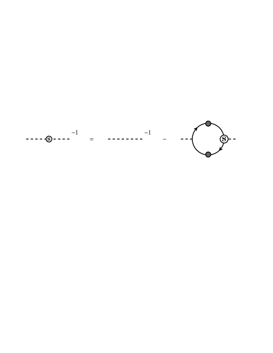
FIG. 2.: The SDE for the scalar propagator $\Delta_{\rm S}(p)$.

FIG. 3.: The SDE for the scalar vertex ${\Gamma_{\rm S}}(p+q,p)$. The shaded circle with the $2$ represents the two-fermion one-boson irreducible fermion-fermion scattering kernel.

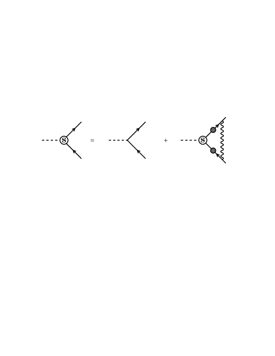
FIG. 4.: The SDE for the scalar vertex in the quenched-ladder approximation.

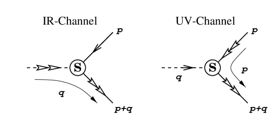
FIG. 5.: The two-channel approximation.

FIG. 6.: A comparison of our result with Appelquist et al. Graphs of ${\rm Im}(\Delta_{\rm S}(p))$ for different values of $\alpha_{0}/\alpha_{c}$. The curves are normalized so that the peak of the $\alpha_{0}/\alpha_{c}=0.01$ curve equals 1.