Abstract. We show that the spectral dimension on non-generic branched polymer models with susceptibility exponent $\gamma>0$ is given by $d_{s}=2/(1+\gamma)$. For those models with $\gamma<0$ we find that $d_{s}=2$.

The spectral dimension $d_{s}$ is an important measure of the dimensionality of the manifold ensembles appearing in quantum gravity. In particular much effort has recently been put into its determination for discretized two-dimensional quantum gravity ensembles. The spectral dimension is defined by a random walk which leaves a fixed vertex at $t=0$ and at every step is allowed to move from its present position to one of its neighbouring vertices with uniform probability. After $t$ steps the probability that the walk has returned to the initial point is given by

$${}P(t)\approx\frac{const}{t^{d_{s}/2}}$$ (1)

provided that $t\gg 1$ (to negate discretization effects) and that $t\ll N^{\Delta}$ where $N$ is the number of vertices in the graph and $\Delta$ some exponent (to avoid finite size effects). The spectral dimension has been investigated numerically for many different values of the central charge $c$ [1] and it has been calculated analytically for the generic branched polymer model [2] and found to be $d_{s}={4\over 3}$ in excellent agreement with the numerical results at large $c$. We refer the reader to refs [1] and [2] for detailed discussion of the definition of $d_{s}$ and the ensemble averages involved. In this letter we extend the results of [2] to the non-generic branched polymers.

We start by recalling the essential features of the branched polymer models [3]. A general branched polymer (BP) model has grand canonical partition function ${\mathcal{Z}}(z)$ satisfying

$${}{\mathcal{Z}}(z)=z(1+\sum_{n=1}^{\infty}\alpha_{n}{\mathcal{Z}}(z)^{n})$$ (2)

where the $\alpha_{n}$ are constants. Iterating this equation shows that ${\mathcal{Z}}(z)$ is the generating function for the set of all rooted trees ${\mathcal{B}}$ made up of links and vertices of all coordination numbers $n+1$ such that $\alpha_{n}\neq 0$,

$${}{\mathcal{Z}}(z)=\sum_{{{\mathrm{A}}}\in{\mathcal{B}}}z^{N_{{\mathrm{A}}}}w_{{\mathrm{A}}}.$$ (3)

The number of links in A is denoted by $N_{{\mathrm{A}}}$ and the weight $w_{{\mathrm{A}}}$ of A is given by

$${}w_{{\mathrm{A}}}=\prod_{v\in{\mathrm{A}}}\alpha_{n(v)-1}$$ (4)

where $v$ runs over all vertices of A and $n(v)$ denotes the coordination number of $v$. We denote the set of all polymers whose first vertex has coordination number $n+1$ by ${\mathcal{B}}^{n}$; clearly ${\mathcal{B}}={\mathcal{B}}^{0}\cup{\mathcal{B}}^{1}\cup{\mathcal{B}}^{2}\cup\ldots$ (${\mathcal{B}}^{0}$ contains the polymer consisting of a single link). Any graph ${\mathrm{A}}\in{\mathcal{B}}^{n}$ has a set of constituents ${\mathrm{A}}_{1},\ldots,{\mathrm{A}}_{n}$ obtained by severing the links connecting the first vertex to the rest of the graph (see fig.1).

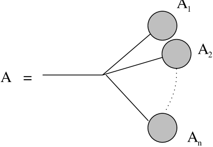
Figure 1: The constituents ${\mathrm{A}}_{1},\ldots,{\mathrm{A}}_{n}$ of a branched polymer ${\mathrm{A}}\in{\mathcal{B}}^{n}$.

Note that for ${\mathrm{A}}\in{\mathcal{B}}^{n}$

$${}w_{{\mathrm{A}}}=\alpha_{n}\prod_{i=1}^{n}w_{{{\mathrm{A}}}_{i}}$$ (5)

and

$${}N_{{\mathrm{A}}}=1+\sum_{i=1}^{n}N_{{{\mathrm{A}}}_{i}}.$$ (6)

Equation (2) can be rewritten in the form

$$\frac{1}{z} = {\mathcal{F}}({\mathcal{Z}})$$ (7)

$${\mathcal{F}}(x) = x^{-1}(1+\sum_{n=1}^{\infty}\alpha_{n}x^{n}).$$ (8)

For small enough $z$ the solution ${\mathcal{Z}}(z)$ is an analytic function but at some critical value $z=z_{{\mathrm{c}}{\mathrm{r}}}$ it is non-analytic; this is the point at which the graphical expansion (3) diverges. The susceptibilty is given by

$${}\chi(z)=\frac{\partial{\mathcal{Z}}}{\partial z}=-\frac{z^{-2}}{{\mathcal{F}}^{\prime}({\mathcal{Z}}(z))}=\frac{{\mathcal{Z}}z^{-1}}{1-z\sum_{n=1}^{\infty}n\alpha_{n}{\mathcal{Z}}(z)^{n-1}}$$ (9)

and so the critical point is where ${\mathcal{F}}^{\prime}({\mathcal{Z}}(z_{{\mathrm{c}}{\mathrm{r}}}))=0$. As $z\to z_{{\mathrm{c}}{\mathrm{r}}}$ the susceptibility has leading non-analytic behaviour given by

$${}\chi(z)\simeq(z_{{\mathrm{c}}{\mathrm{r}}}-z)^{-\gamma}$$ (10)

where $\gamma$ is the susceptibility exponent. (Throughout this letter we use the symbol $\simeq$ to denote the leading singularity as $z\to z_{{\mathrm{c}}{\mathrm{r}}}$.) The nature of the critical point and the value of $\gamma$ depend upon how ${\mathcal{F}}^{\prime}$ vanishes. The multi-critical BPs are obtained by supposing that ${\mathcal{F}}^{(n)}({\mathcal{Z}}(z_{{\mathrm{c}}{\mathrm{r}}}))=0,\>n=0,\ldots k$ but that ${\mathcal{F}}^{(k+1)}({\mathcal{Z}}(z_{{\mathrm{c}}{\mathrm{r}}}))\neq 0$ so, close to $z_{{\mathrm{c}}{\mathrm{r}}}$,

$${}\chi(z)\simeq\frac{z^{-2}}{|{\mathcal{Z}}(z)-{\mathcal{Z}}(z_{{\mathrm{c}}{\mathrm{r}}})|^{k}}\;.$$ (11)

However

$${}{\mathcal{Z}}(z)\simeq{\mathcal{Z}}(z_{{\mathrm{c}}{\mathrm{r}}})-const.(z_{{\mathrm{c}}{\mathrm{r}}}-z)^{1-\gamma}$$ (12)

so comparing singularities we obtain

$$\gamma = k(1-\gamma)$$

$${\mathrm{or}}\quad\gamma = 1-\frac{1}{k+1}\;.$$ (13)

The generic case, requiring no special tuning of the $\alpha_{n}$ (except that at least one $\alpha_{n}$ ($n\geq 2$) must be non-zero), is $k=1$, $\gamma={1\over 2}$; higher values of $k$, which require at least $k$ of the $\alpha_{n}$ ($n\geq 2$) to be non-zero and of varying sign to enforce the vanishing of higher derivatives, give the multi-critical BPs (MCBP from now on).

The MCBPs are not the only ones with $\gamma\neq{1\over 2}$. By allowing an infinite number of the $\alpha_{n}$ to be non-zero we can arrange that ${\mathcal{F}}^{\prime}$ vanishes non-analytically [4, 5]. Consider

$${}{\mathcal{F}}({\mathcal{Z}})=\frac{1}{{\mathcal{Z}}}+\mu+\frac{{\mathcal{Z}}}{A^{2}}+\lambda\left(1-\frac{{\mathcal{Z}}}{A}\right)^{\beta+1}$$ (14)

where $A$, $\lambda$, $\mu$ and $\beta$ are positive constants. Then

$${}{\mathcal{F}}^{\prime}({\mathcal{Z}})=-\frac{1}{{\mathcal{Z}}^{2}}+\frac{1}{A^{2}}-\frac{\lambda(\beta+1)}{A}\left(1-\frac{{\mathcal{Z}}}{A}\right)^{\beta}.$$ (15)

As $z$ increases from zero so does ${\mathcal{Z}}(z)$. The first zero of ${\mathcal{F}}^{\prime}$ is at ${\mathcal{Z}}=A$ when $z_{{\mathrm{c}}{\mathrm{r}}}=(2/A+\mu)^{-1}$; provided that $1>\beta>0$ the non-analytic term in (15) dominates as $z\to z_{{\mathrm{c}}{\mathrm{r}}}$. Inserting this dominant behaviour into (11), using (12), and comparing singularities, we obtain

$${}\gamma=\frac{\beta}{\beta+1}.$$ (16)

Thus we get models with continuously varying $\gamma$ in the range 0 to ${1\over 2}$ as discussed in [5]. However the restriction on the range of $\beta$ is easily removed; by tuning the coefficients $\alpha_{n}$ so that the analytic part of ${\mathcal{F}}^{\prime}$ in (15) vanishes as $({\mathcal{Z}}-A)^{2}$ the non-analytic behaviour dominates for $2>\beta>0$ so now we can get continuously varying $\gamma$s up to ${2\over 3}$. If the coefficients are tuned so that the analytic part of ${\mathcal{F}}^{\prime}$ in (15) vanishes as $({\mathcal{Z}}-A)^{m}$ then $\beta$ can be as large as $m$. In this way we see that by combining the multi-critical strategy and the non-analytic form of ${\mathcal{F}}$ used in [4, 5] we can obtain all $\gamma$ values in the range 0 to 1. If $\beta$ is an integer these models just reproduce the MCBP; when $\beta$ is not an integer we will call them the ‘continuous critical branched polymers’, or CCBP.

The CCBPs actually continue to negative gamma. Suppose that ${\mathcal{F}}^{\prime}$ is finite at $z_{{\mathrm{c}}{\mathrm{r}}}$ but that ${\mathcal{F}}^{\prime\prime}$ diverges; then by (9) the susceptibility $\chi$ is finite at $z_{{\mathrm{c}}{\mathrm{r}}}$. However

$${}\frac{\partial\chi}{\partial z}=\frac{2z^{-3}}{{\mathcal{F}}^{\prime}({\mathcal{Z}}(z))}+\frac{z^{-2}{\mathcal{F}}^{\prime\prime}({\mathcal{Z}}(z))\chi}{{\mathcal{F}}^{\prime}({\mathcal{Z}}(z)^{2})}$$ (17)

so the derivative of $\chi$ diverges at the critical point and $\gamma$ is negative. This is easily arranged by (for example) eliminating the linear term in (14) so that

$${}{\mathcal{F}}({\mathcal{Z}})=\frac{1}{{\mathcal{Z}}}+\mu+\lambda\left(1-\frac{{\mathcal{Z}}}{A}\right)^{\beta+1}$$ (18)

with $1>\beta>0$ and comparison of the behaviour as $z\to z_{{\mathrm{c}}{\mathrm{r}}}$ then gives

$${}\gamma=\frac{-\beta}{2-\beta}.$$ (19)

In our calculation of the spectral dimension we will need to know the behaviour of

$${}\Omega_{l}=\frac{d^{l+1}}{d{\mathcal{Z}}^{l+1}}\sum_{n=1}^{\infty}\alpha_{n}{\mathcal{Z}}(z)^{n}=\frac{d^{l+1}}{d{\mathcal{Z}}^{l+1}}{\mathcal{Z}}{\mathcal{F}}({\mathcal{Z}})$$ (20)

close to the critical point. Using the properties of ${\mathcal{F}}$ discussed above we find that for $\gamma>0$

$$\Omega_{l} \simeq ({\mathcal{Z}}(z)-{\mathcal{Z}}(z_{{\mathrm{c}}{\mathrm{r}}}))^{\beta-l}+\frac{1}{z_{{\mathrm{c}}{\mathrm{r}}}}\delta_{l,0}$$ (21)

$$= (z_{{\mathrm{c}}{\mathrm{r}}}-z)^{\gamma-l(1-\gamma)}+\frac{1}{z_{{\mathrm{c}}{\mathrm{r}}}}\delta_{l,0}$$

unless $\beta$ is an integer (ie MCBP) in which case for $l\geq\beta$ we find that $\Omega_{l}$ is finite at $z_{{\mathrm{c}}{\mathrm{r}}}$. If $\gamma<0$ then ${\mathcal{F}}^{\prime}$ is finite and it follows from (9) that

$${}1-z_{{\mathrm{c}}{\mathrm{r}}}\Omega_{0}(z_{{\mathrm{c}}{\mathrm{r}}})=C$$ (22)

where $C$ is finite.

Our calculation of the spectral dimension follows the same method as in [2] but generalized to take account of the presence of vertices of varying order. The return probability generating function $P_{{\mathrm{A}}}(y)$ on a given polymer ${\mathrm{A}}\in{\mathcal{B}}^{n}$ is related to that on its $n$ constituents ${\mathrm{A}}_{1},\ldots{\mathrm{A}}_{n}$ (see fig.1). It is convenient to define for any polymer ${\mathrm{A}}\in{\mathcal{B}}$

$${}P_{{\mathrm{A}}}(y)=\frac{1}{1-y}\frac{1}{h_{{\mathrm{A}}}(y)}$$ (23)

and then we find for ${\mathrm{A}}\in{\mathcal{B}}^{n}$ [2]

$${}h_{{\mathrm{A}}}(y)=\frac{1+\sum_{i=1}^{n}h_{{{\mathrm{A}}}_{i}}(y)}{1+(1-y)\sum_{i=1}^{n}h_{{{\mathrm{A}}}_{i}}(y)}.$$ (24)

Note that at $y=1$ the solution is

$${}h_{{\mathrm{A}}}(1)=N_{{\mathrm{A}}}$$ (25)

for all polymers ${\mathrm{A}}\in{\mathcal{B}}$. The spectral dimension is found by considering the quantity

$${}{\widetilde{{\mathcal{Q}}}}(z,y)=-\frac{d}{dy}(1-y)\sum_{{\mathrm{A}}\in{\mathcal{B}}}z^{N_{{\mathrm{A}}}}w_{{\mathrm{A}}}P_{{\mathrm{A}}}(y)=\frac{d}{dy}\sum_{{\mathrm{A}}\in{\mathcal{B}}}\frac{z^{N_{{\mathrm{A}}}}w_{{\mathrm{A}}}}{h_{{\mathrm{A}}}(y)}.$$ (26)

At $y=1$ the $n$th derivative with respect to $y$ of ${\widetilde{{\mathcal{Q}}}}(z,y)$ behaves as

$${}{\widetilde{{\mathcal{Q}}}}_{n}(z)=\frac{\partial^{n}}{\partial y^{n}}{\widetilde{{\mathcal{Q}}}}(z,y){\Bigg{|}_{y=1}}\simeq(z_{{\mathrm{c}}{\mathrm{r}}}-z)^{\beta-n\Delta}$$ (27)

where the exponents $\beta$ and $\Delta$ are related to the spectral dimension by

$${}\beta=1-\gamma+\Delta(d_{s}/2-1).$$ (28)

The behaviour (27) can be established by considering the quantities

$${}H^{(n_{1},n_{2},\ldots,n_{p})}=\sum_{{\mathrm{A}}\in{\mathcal{B}}}z^{N_{{\mathrm{A}}}}w_{{\mathrm{A}}}\prod_{i=1}^{p}\frac{d^{n}}{dy^{n}}h_{{\mathrm{A}}}(y){\Bigg{|}_{y=1}}$$ (29)

which have leading singular behaviour as $z\to z_{{\mathrm{c}}{\mathrm{r}}}$ given by [2]

$${}H^{(n_{1},n_{2},\ldots,n_{p})}\simeq(z_{{\mathrm{c}}{\mathrm{r}}}-z)^{a-bp-c\sum_{i=1}^{p}n_{i}}$$ (30)

where we will determine the constants a,b,c.

First we will consider the case when $\gamma>0$. Let us compute

$$H^{(1)} = \sum_{{\mathrm{A}}\in{\mathcal{B}}}z^{N_{{\mathrm{A}}}}w_{{\mathrm{A}}}h^{\prime}_{{\mathrm{A}}}(1)$$ (31)

$$= \sum_{n}\sum_{{\mathrm{A}}\in{\mathcal{B}}^{n}}z^{N_{{\mathrm{A}}}}w_{{\mathrm{A}}}h^{\prime}_{{\mathrm{A}}}(1).$$

Now we use (24) to relate $h^{\prime}_{{\mathrm{A}}}$ to the corresponding quantity for the constituents of ${\mathrm{A}}$ and (4) to relate the weights and obtain

$$H^{(1)} = \sum_{n}\alpha_{n}\sum_{{\mathrm{A}}\in{\mathcal{B}}^{n}}\sum_{{\mathrm{A}}_{1}\cup{\mathrm{A}}_{2}\cup\ldots{\mathrm{A}}_{n}={\mathrm{A}}}z^{1+N_{{{\mathrm{A}}}_{1}}+\ldots N_{{{\mathrm{A}}}_{n}}}w_{{{\mathrm{A}}}_{1}}\ldots w_{{{\mathrm{A}}}_{n}}$$ (32)

$$\left\{\sum_{i=1}^{n}h^{\prime}_{{{\mathrm{A}}}_{i}}(1)+\sum_{i=1}^{n}h_{{{\mathrm{A}}}_{i}}(1)\left(1+\sum_{j=1}^{n}h_{{{\mathrm{A}}}_{j}}(1)\right)\right\}.$$

Note that although ${\mathrm{A}}\in{\mathcal{B}}^{n}$ in the above expression there is no such restriction on its constituent polymers, ${\mathrm{A}}_{i}\ldots{\mathrm{A}}_{n}$ which are drawn from the entire ensemble ${\mathcal{B}}$. The terms on the r.h.s. of (32) which involve $h_{{{\mathrm{A}}}_{m}}^{\prime}(1)$, of which there are $n$, simply reproduce $H^{(1)}$ multiplied by powers of the partition function; by using (25) we see that the remaining pieces simply produce derivatives of the partition function so we may rearrange (32) to obtain

$${}H^{(1)}\left(1-z\sum_{n=1}^{\infty}n\alpha_{n}{\mathcal{Z}}(z)^{n-1}\right)=z^{2}\frac{\partial^{2}}{\partial z^{2}}{\mathcal{Z}}.$$ (33)

The coefficient of $H^{(1)}$ is $1-z\Omega_{0}$ so by (10) and (21) we obtain

$${}H^{(1)}\simeq(z_{{\mathrm{c}}{\mathrm{r}}}-z)^{-1-2\gamma}$$ (34)

and also, since $H^{(1)}$ is the second derivative of ${\widetilde{{\mathcal{Q}}}}_{0}(z)$ with respect to $z$, that

$${}{\widetilde{{\mathcal{Q}}}}_{0}(z)\simeq(z_{{\mathrm{c}}{\mathrm{r}}}-z)^{1-2\gamma}$$ (35)

which gives $\beta=1-2\gamma$.

Next we compute

$$H^{(1,1)} = \sum_{{\mathrm{A}}\in{\mathcal{B}}}z^{N_{{\mathrm{A}}}}w_{{\mathrm{A}}}h^{\prime}_{{\mathrm{A}}}(1)h^{\prime}_{{\mathrm{A}}}(1)$$ (36)

$$= \sum_{n}\alpha_{n}\sum_{{\mathrm{A}}\in{\mathcal{B}}^{n}}\sum_{{\mathrm{A}}_{1}\cup{\mathrm{A}}_{2}\cup\ldots{\mathrm{A}}_{n}={\mathrm{A}}}z^{1+N_{{{\mathrm{A}}}_{1}}+\ldots N_{{{\mathrm{A}}}_{n}}}w_{{{\mathrm{A}}}_{1}}\ldots w_{{{\mathrm{A}}}_{n}}\left\{\sum_{i=1}^{n}h^{\prime}_{{{\mathrm{A}}}_{i}}(1)\right\}^{2}$$

$$+2z^{2}\frac{\partial^{2}}{\partial z^{2}}\sum_{n}\alpha_{n}\sum_{{\mathrm{A}}\in{\mathcal{B}}^{n}}\sum_{{\mathrm{A}}_{1}\cup{\mathrm{A}}_{2}\cup\ldots{\mathrm{A}}_{n}={\mathrm{A}}}z^{1+N_{{{\mathrm{A}}}_{1}}+\ldots N_{{{\mathrm{A}}}_{n}}}w_{{{\mathrm{A}}}_{1}}\ldots w_{{{\mathrm{A}}}_{n}}\left\{\sum_{i=1}^{n}h^{\prime}_{{{\mathrm{A}}}_{i}}(1)\right\}$$

$$+\left(z^{2}\frac{\partial^{2}}{\partial z^{2}}\right)^{2}{\mathcal{Z}}.$$

Again the first sum contains pieces which reproduce $H^{(1,1)}$; the remaining terms on the r.h.s. of (36) can be expressed in terms of $H^{(1)}$ and ${\mathcal{Z}}$. We obtain

$$H^{(1,1)}\left(1-z\sum_{n=1}^{\infty}n\alpha_{n}{\mathcal{Z}}(z)^{n-1}\right) = z\sum_{n=2}^{\infty}n(n-1)\alpha_{n}{\mathcal{Z}}^{n-2}\left(H^{(1)}\right)^{2}$$ (37)

$$+2z^{2}\frac{\partial^{2}}{\partial z^{2}}z\sum_{n=1}^{\infty}n\alpha_{n}{\mathcal{Z}}(z)^{n-1}H^{(1)}$$

$$+\left(z^{2}\frac{\partial^{2}}{\partial z^{2}}\right)^{2}{\mathcal{Z}}.$$

Noting that the coefficient of the $\left(H^{(1)}\right)^{2}$ term is simply $z\Omega_{1}$ and that the coefficient of the $H^{(1)}$ term is $z\Omega_{0}$ which tends to 1 as $z\to z_{{\mathrm{c}}{\mathrm{r}}}$ we see that the first two terms on the r.h.s. of (37) both vary as $(z_{{\mathrm{c}}{\mathrm{r}}}-z)^{-3-2\gamma}$ whilst the last term is sub-leading since it varies as $(z_{{\mathrm{c}}{\mathrm{r}}}-z)^{-3-\gamma}$. The coefficient of $H^{(1,1)}$ varies, as before, like $(z_{{\mathrm{c}}{\mathrm{r}}}-z)^{\gamma}$ so we find

$${}H^{(1,1)}\simeq(z_{{\mathrm{c}}{\mathrm{r}}}-z)^{-3-3\gamma}.$$ (38)

We can iterate this process; $H^{(1,1,1)}$ is given by

$$H^{(1,1,1)}\left(1-z\Omega_{0}\right) = z\Omega_{2}\left(H^{(1)}\right)^{3}+z\Omega_{1}H^{(1,1)}H^{(1)}+3z^{2}\frac{\partial^{2}}{\partial z^{2}}z\Omega_{0}H^{(1,1)}$$ (39)

$$+\,\hbox{(less singular terms)}.$$

The presence of the coefficients $\Omega_{1,2}$ in the first two terms on the r.h.s. changes their degree of divergence to $(z_{{\mathrm{c}}{\mathrm{r}}}-z)^{-5-3\gamma}$ which is the same as that of the third term and hence we conclude that

$${}H^{(1,1,1)}\simeq(z_{{\mathrm{c}}{\mathrm{r}}}-z)^{-5-4\gamma}.$$ (40)

This process may be continued to longer strings $(1,1,1,\ldots,1)$ and to strings involving higher derivatives of $h_{{\mathrm{A}}}(y)$ (obtained by successive differentiation of (24)). Following [2] we can set up a proof by induction [6] that

$${}H^{(n_{1},n_{2},\ldots,n_{p})}\simeq(z_{{\mathrm{c}}{\mathrm{r}}}-z)^{1-\gamma-p-(1+\gamma)\sum_{i=1}^{p}n_{i}}$$ (41)

from which it follows, by inserting this result in (27) (see [2] for details), that $\Delta=1+\gamma$. Substituting this and $\beta=1-2\gamma$ into (28) we find that

$${}d_{s}=\frac{2}{1+\gamma}.$$ (42)

Note that the spectral dimension also satisfies the scaling relation $d_{s}\Delta=2$. As was discussed in [7] this scaling relation is expected to be true for graphs whose Laplacian has no level-dependent degeneracy in its eigenvalue spectrum; clearly the BP ensembles, most of whose graphs have no symmetries, fall into this category.

The case of $\gamma<0$ is simpler. The factor $1-z\Omega_{0}$ does not vanish as $z\to z_{{\mathrm{c}}{\mathrm{r}}}$ so we now find that

$${}H^{(1)}\simeq(z_{{\mathrm{c}}{\mathrm{r}}}-z)^{-1-\gamma}$$ (43)

and therefore that

$${}{\widetilde{{\mathcal{Q}}}}_{0}(z)\simeq(z_{{\mathrm{c}}{\mathrm{r}}}-z)^{1-\gamma}$$ (44)

which implies $\beta=1-\gamma$. Using (28) we see immediately that $d_{s}=2$. Of course it is necessary to check that $\Delta\neq 0$ before reaching this conclusion; in fact it is straightforward to show that $\Delta=1$ [6] and so the scaling relation $d_{s}\Delta=2$ is still satisfied.

It is interesting to compare these results with a scaling relation recently found by Ambjørn et al [8]. They showed that

$${}\frac{2}{d_{H}}=\Delta\left(1-\frac{d_{s}}{2}\right)$$ (45)

where $d_{H}$ is the extrinsic Hausdorff dimension. For the $k$th multicritical model $d_{H}$ has been calculated [3] and is known to be given by

$${}d_{H}=\frac{2(k+1)}{k}.$$ (46)

Assuming that $d_{s}\Delta=2$ we can then use (45) to determine that [8]

$${}d_{s}=\frac{2}{2-\frac{1}{k+1}}=\frac{2}{1+\gamma}$$ (47)

in agreement with our calculations. The value of $d_{H}$ has not been calculated explicitly for the CCBPs but we can now use the scaling relation (45) and our results to show that $\gamma d_{H}=2$ if $\gamma>0$. When $\gamma<0$ we have $d_{s}=2$ so we expect $d_{H}=\infty$. It is amusing that the two-dimensional quantum gravity models at $c<1$ also have $d_{H}=\infty$ and hence $d_{s}=2$ [8].

We acknowledge valuable conversations with Jan Ambjørn who told us of the scaling relation result (45) prior to writing the paper [8]. J.C. acknowledges a grant from Praxis XXI.

References

[1] J.Ambjørn, J.Jurkiewicz and Y.Watabiki, Nucl. Phys. B454
(1995) 313.
[2]T. Jonsson and J.F. Wheater, “The spectral dimension of the
branched polymer phase of two dimensional quantum gravity”, Oxford University Preprint OUTP-97-33P, hep-lat/9710024.
[3]J.Ambjørn, B.Durhuus and T.Jonsson, Phys. Lett. B244
(1990) 403.
[4]J.Ambjørn, B. Durhuus, J. Fröhlich and P.Orland,
Nucl. Phys. B270 [FS16] 457.
[5]P. Bialas and Z. Burda, Phys. Lett. B 384 (1996) 75.
[6]J.D. Correia, D.Phil Thesis, Oxford University 1998.
[7]T. Jonsson and J.F. Wheater, “The spectral dimension
on branched polymer ensembles”, to appear in the proceedings of NATO
workshop
New Developments in Quantum Field Theory, eds. P.H. Damgaard and
J. Jurkiewicz, published by Plenum Publishing Corp., New York.
[8]J. Ambjørn, D. Boulatov, J.L. Nielsen, J. Rolf and Y. Watabiki, “The spectral dimension of 2d quantum gravity”, Niels Bohr Institute preprint NBI-HE-97-62.