Theoretical Physics Institute
University of Minnesota

OUTP-97-70-P

TPI-MINN-97/27-T

UMN-TH-1611-97

hep-th/9712046

More on Supersymmetric Domain Walls, $N$ Counting and Glued Potentials

Ian I. Kogan, Alex Kovner

Theoretical Physics, Oxford University. 1 Keble Road, Oxford OX13NP, UK

and

Mikhail Shifman

Theoretical Physics Institute, Univ. of Minnesota, Minneapolis, MN 55455, USA

Various features of domain walls in supersymmetric gluodynamics are discussed. We give a simple field-theoretic interpretation of the phenomenon of strings ending on the walls recently conjectured by Witten. An explanation of this phenomenon in the framework of gauge field theory is outlined. The phenomenon is argued to be particularly natural in supersymmetric theories which support degenerate vacuum states with distinct physical properties. The issue of existence (or non-existence) of the BPS saturated walls in the theories with glued (super)potentials is addressed. The amended Veneziano–Yankielowicz effective Lagrangian belongs to this class. The physical origin of the cusp structure of the effective Lagrangian is revealed, and the limitation it imposes on the calculability of the wall tension is explained. Related problems are considered. In particular, it is shown that the so called discrete anomaly matching, when properly implemented, does not rule out the chirally symmetric phase of supersymmetric gluodynamics, contrary to recent claims.

1 Introduction

Recently there have been a renewed interest in the study of theoretical aspects of $N=1$ supersymmetric (SUSY) gauge theories. In addition to the calculation of exact effective potentials [1] and conjectured dualities between theories with distinct gauge groups [2], it has been realized that in some supersymmetric theories there exists a class of dynamical objects whose energy can be calculated exactly [3]. Those are the domain walls interpolating between discrete vacua which are typical for many SUSY gauge theories. The remarkable fact is that the energy density (tension) of these walls is exactly calculable even in the strong coupling regime.

For supersymmetric gluodynamics, the theory of gluons and gluinos with no matter, the calculation of the energy density was carried out in Ref. [3], in an indirect way. The key ingredient is the central extension of the $N=1$ superalgebra,

$$\{Q^{\dagger}_{\dot{\alpha}}Q^{\dagger}_{\dot{\beta}}\}=\frac{N}{4\pi^{2}}\left(\vec{\sigma}\right)_{\dot{\alpha}\dot{\beta}}\int\,d^{3}x\,\vec{\nabla}\left(\mbox{Tr}\,\lambda^{2}\right)\,,$$ (1)

where $Q^{\dagger}_{\dot{\alpha}}$ is the supercharge, $\lambda$ is the gluino field, and $\left(\vec{\sigma}\right)_{\dot{\alpha}\dot{\beta}}=\{\sigma^{3},-i,-\sigma^{1}\}_{\dot{\alpha}\dot{\beta}}$ is a set of matrices converting the vectorial index of the representation $(1,0)$ of the Lorentz group in the spinorial indices. The commutator (1) is given for $SU(N)$ gauge group; the parameter $N$ stands for the number of colors. The right-hand side of Eq. (1) is a reflection of “geometric” anomalies of SUSY gluodynamics (i.e. that in the trace of the energy-momentum tensor plus its supergeneralizations).

The integral over the full derivative on the right-hand side is zero for all localized field configurations. It does not vanish, however, for the domain walls. Equation (1) implies that the tension of the domain wall is

$$\varepsilon=\frac{N}{8\pi^{2}}\left|\langle\mbox{Tr}\,\lambda^{2}\rangle_{\infty}-\langle\mbox{Tr}\,\lambda^{2}\rangle_{-\infty}\right|\,,$$ (2)

where the subscript $\pm\infty$ marks the values of the gluino condensate at spatial infinities (say, at $z\rightarrow\pm\infty$ assuming that the domain wall lies in the $xy$ plane). The existence of the exact relation (2) is a consequence of the fact that the domain wall in the case at hand is a BPS-saturated configuration preserving $1/2$ of the original supersymmetry. A general discussion of BPS saturated domain walls was given in [4], while a particular wall realization in the framework of the amended [5] Veneziano–Yankielowicz effective Lagrangians [6] were studied in some detail in [7] and [8].

On the other hand, a theory related to supersymmetric gluodynamics was analyzed recently from the point of view of $D$-brane physics [9]. In this picture the domain walls also appear naturally. Moreover they seem to have some rather surprising properties. These properties are natural from the $D$-brane perspective but were considered unusual (even paradoxical) from the field-theoretical point of view [9]. One of such features is an “abnormal” $N$ dependence of the wall tension. The wall energy density of some BPS saturated walls scales as $N$, rather than $N^{2}$, a dependence one might expect apriori from glueball solitons. The second surprise [9] is that the confining QCD string emanating from the probe color charges (quarks) on one side of the wall can terminate on the wall, without penetrating on the other side.

So far these features had no satisfactory explanation in the field-theoretical framework. One of our tasks is to understand how this works in field theory, at least at a qualitative level. We show that both aspects – the $N$ dependence and termination of the flux tubes on the walls – are quite natural consequences of the peculiar gauge dynamics. We suggest various toy models, which are simpler than SUSY gluodynamics but still carry essential features of the phenomena under discussion, to substantiate our qualitative observations. For instance, an Abelian model is presented where probe fractional charges generate induced “mirror” fractional charges on the wall in spite of the fact that at the fundamental level the model contains no fractionally charged fields.

Then we turn to the Veneziano–Yankielowicz effective Lagrangians. Previously they were exploited as a framework for quantitative analysis of the domain walls [7]. A BPS wall interpolating between a chirally symmetric vacuum [5] and one of the conventional vacua with $\langle\lambda\lambda\rangle\neq 0$ was explicitly built. However, building a wall interpolating between two neighboring chirally asymmetric vacua turned out to be a much harder endeavor. The task had not been solved in Ref. [7]. Moreover, it was argued later [8] that such walls do not exist within the framework of the Veneziano–Yankielowicz effective Lagrangians.

A crucial feature of such a Lagrangian emerging in SUSY gluodynamics is discontinuity of the superpotential ${\cal W}$. The realization compatible with all symmetries of the underlying theory requires, with necessity, a “glued” potential [5], with $N$ distinct sectors and matching lines along the boundaries of the sectors. We explain the physical nature of this phenomenon. The sector pattern, with cusps, reflects a restructuring of heavy degrees of freedom (which were integrated out) in the process of an adiabatic variation of the light degrees of freedom. A level crossing takes place in the heavy sector of the theory. Precisely for this reason, one cannot construct the domain wall from the effective Lagrangian if the wall crosses the cusp. The presence of the cusps prevents one from being able to use this potential for calculating a wall profile if the field configuration along the wall crosses the cusp somewhere in space. In fact, if one naively tries to do this in the presence of the cusp an apparent paradox arises – the wall in the effective theory seems to have a lower energy density than the BPS bound on this quantity in the original theory. The missing energy density is contributed by the excitation of the heavy modes which are necessarily excited when the light fields take values in the vicinity of the cusp.

The statement is thoroughly illustrated by two toy models. The phenomenon is quite general and may be considered in supersymmetric as well as non-supersymmetric context.

The chirally symmetric vacuum, $\langle\lambda\lambda\rangle=0$, is inherent to the Veneziano–Yankielowicz Lagrangian. Recently it was claimed [10] that a discrete anomaly matching rules out the existence of such phase, at least its most straightforward realization. We make a digression to show that the claim is due to an inconsistent treatment of the discrete anomaly matching. In SUSY gluodynamics and similar theories the discrete anomaly matching imposes no constraints on the spectrum. The only information one gets are rather mild constrains on certain amplitudes following from the classical symmetries that become anomalous at the quantum level (see e.g. [11]). The existence of a discrete anomaly-free subgroup adds no new information.

The organization of the paper is as follows. Section 2 is devoted to general aspects of the BPS walls in SUSY gluodynamics. We analyze, qualitatively, the $N$ dependence of the wall tension and visualize the phenomenon of strings ending on the domain walls. An analogy between the walls in SUSY gluodynamics and the axion domain walls in gauge theories with monopoles is worked out.

In Sect. 3 we turn to a more quantitative discussion based on the amended Veneziano–Yankielowicz effective action. The issue of glued potentials is studied here. In Sect. 3.3 we consider an explicit example of a supersymmetric theory which upon integrating out heavy modes generates an effective potential with cusps. In this model we calculate explicitly the cusp contribution to the wall tension and show how the apparent contradiction with the BPS bound is resolved. In Sect. 3.4 aspects of the general theory of glued (super)potentials are presented.

In Sect. 4 we discuss other domain walls in gauge theories obtained as a Kaluza-Klein reduction on topologically non-trivial space-time manifolds. The specific example considered refers to $R_{4}\times S_{1}$. An unconventional $N$ dependence of the wall tension arises which may be related to $D$-branes.

Section 5 is devoted to the issue of the discrete anomaly matching and the chirally symmetric vacuum of SUSY gluodynamics.

Finally, Sect. 6 contains a brief summary and discussion of our results.

2 $N$ Dependence, Flux Tubes Ending on the Walls and All That

2.1 SUSY Gluodynamics

We consider the supersymmetric generalization of pure gluodynamics – i.e. the theory of gluons and gluinos. At the fundamental level the Lagrangian of the model has the form [12]

$${\cal L}=-\frac{1}{4g_{0}^{2}}G_{\mu\nu}^{a}G_{\mu\nu}^{a}+{\vartheta\over 32\pi^{2}}G_{\mu\nu}^{a}\tilde{G}_{\mu\nu}^{a}+\frac{1}{g_{0}^{2}}\left[i\lambda^{a\alpha}D_{\alpha\dot{\beta}}\bar{\lambda}^{a\dot{\beta}}\right]\,,$$ (3)

where the spinorial notation is used. In the superfield language the Lagrangian can be written as

$${\cal L}=\frac{1}{4g^{2}}\mbox{Tr}\int d^{2}\theta W^{2}+\,\mbox{H.c.}\,,$$ (4)

where

$$\frac{1}{g^{2}}=\frac{1}{g_{0}^{2}}-\frac{i\vartheta}{8\pi^{2}}\,.$$

Here $\vartheta$ denotes the vacuum angle. Our conventions regarding the superfield formalism are summarized e.g. in the recent review [13]. We will limit ourselves to the $SU(N)$ gauge group (the generators of the group $T^{a}$ are in the fundamental representation, so that $\mbox{Tr}(T^{a}T^{b})=(1/2)\delta^{ab}$).

$SU(N)$ supersymmetric gluodynamics has a discrete symmetry, $Z_{2N}$, a (non-anomalous) remnant of the anomalous axial symmetry generated by the phase rotations of the gluino field. The gluino condensate $\langle\lambda\lambda\rangle$ is the order parameter of this symmetry. The discrete chiral symmetry may or may not be spontaneously broken [5]. Therefore, there exists a set of distinct vacua labeled by the value of the gluino condensate. In the phase with the broken chiral symmetry Tr$\langle\lambda\lambda\rangle=\Lambda^{3}\exp(2\pi ik/N)$ where $k=0,1,2,...,N-1$ (for $\vartheta=0$). In the chirally symmetric phase Tr$\langle\lambda\lambda\rangle=0$. The field configurations interpolating between different values of $\langle\lambda\lambda\rangle$ at spatial infinities are topologically stable domain walls. Although the theory is in the strong coupling regime one can derive an exact lower bound on the surface energy density (tension) for such a wall [3]

$$\varepsilon\geq\frac{N}{8\pi^{2}}\left|\langle\mbox{Tr}\,\lambda^{2}\rangle_{\infty}-\langle\mbox{Tr}\,\lambda^{2}\rangle_{-\infty}\right|\,.$$ (5)

In our normalization the condensate $\langle\mbox{Tr}\,\lambda^{2}\rangle$ scales as $N$ in the large $N$ limit.

One may consider two types of walls. The wall of type I connects a vacuum with the spontaneously broken chiral symmetry with the symmetric vacuum ($\langle\mbox{Tr}\,\lambda^{2}\rangle=0$). For such a wall the BPS bound for the tension is

$$\varepsilon\sim O(N^{2})\,.$$

The walls of type II connect two adjacent (or close) chirally asymmetric vacua, e.g. $k=0$ and $k=1$ (or $k=0$ and $k=2$, etc.). Even though for each of these vacua the order parameter is of order $N$, the difference between the order parameters is $O(1)$. The BPS bound for the tension, therefore, is

$$\varepsilon\sim O(N)\,.$$

Let us assume for the moment that the BPS-saturated walls of type II do indeed exist in SUSY gluodynamics. Although we cannot prove this at present, there are no visible reasons forbidding them .

The question then arises as to how one can understand the large $N$ scaling of the wall energy density from the point of view of the effective field theory which describes dynamics of the low lying physical states, mesons and glueballs and their superpartners.

At large $N$ the mesons and the glueballs should have masses of order 1, trilinear couplings of order $1/N$, and so on [14]. This is conveniently encoded in an effective Lagrangian of the form

$${\cal L}=N^{2}F[M_{i},\partial M_{i}]\,,$$ (6)

where $\{M_{i}\}$ is a set of fields representing all relevant degrees of freedom, mesons and glueballs. The value of the functional $F$ itself and all its derivatives at the minima should be independent of $N$. This would ensure the proper $N$ dependence of the masses and coupling constants. Now, suppose we have a solution of classical equations of motion $M_{\rm wall}$ which describes a wall configuration interpolating between two distinct minima. Since $N^{2}$ is an overall factor in Eq. (6), at first sight one may expect that $F[M_{\rm wall}]=O(1)$, and, therefore, the wall tension $\varepsilon=O(N^{2})$. Such a situation is standard in the soliton physics. This is perfectly in line with what we get for the type I walls, but is in apparent contradiction with the BPS energy density of the type II wall.

Can one avoid this conclusion? The answer is yes. Consider a function $F$ which is nonanalytic so that although all its derivatives are $O(1)$ at the minimum $M_{*}$, at some finite distance $M=M_{*}+\delta M$ (with $\delta M=O(1/N)$) the derivatives become large ($O(N)$, for example). Then, if the wall solution $M_{\rm wall}$ passes through this region of the field space, the standard counting leading to $\varepsilon=O(N^{2})$ does not work. An extreme example of such a situation arises if the effective Lagrangian has a structure of $N$ distinct sectors in the space of fields, and no single analytical function $F$ exist. The $N$ sector structure then is an implicit source of $N$ dependence. Such a potential is singular (or rather has a singular first derivative) along the boundaries of the sectors, being glued from different pieces along the boundaries. As we will discuss later, this situation can arise due to the fact that the state that was the ground state in one sector, becomes an excited state in another, and vice versa. At the boundary there are degenerate states, and the level crossing occurs. Due to the cusps at the boundary the naive estimate of the tension presented above does not work in the case of the glued potential. As we will see, the effective potential in SUSY gluodynamics has precisely this $N$–sector structure.

Of course, in the full theory everything is smooth. One can ensure the smoothness of an effective Lagrangian by including more fields in it. Those extra fields will not correspond to low energy excitations in the vicinity of the minima (and therefore will be unimportant for local properties like Green’s functions), but will be essential for smoothing the singularity at the cusps. In the example just discussed one would have to include in the game at least $N$ fields. That is how $N$ enters the effective potential as a hidden parameter (besides the overall $N^{2}$ factor in Eq. (6)). Then the typical value of relevant fields $M_{i}$ inside the wall solution can be $O(N^{-1})$, each field contributes to $F$ at the level $O(N^{-2})$, but there are $N$ relevant fields, and the value of $F\sim 1/N$. Note that the wall width is $L\sim N^{0}$. Then the volume energy density inside the wall $E\sim N$ and, correspondingly, the wall tension $\varepsilon\sim N$.

The fact that the volume energy $E$ is $O(N)$ inside the BPS wall connecting two neighboring vacua, say with Tr$\langle\lambda\lambda\rangle=\Lambda^{3}\exp(2\pi ik/N)$ where $k=0$ and 1, is seen in the microscopic theory (3) per se. Indeed, for the BPS wall

$$G_{\mu\nu}^{a}G_{\mu\nu}^{a}\sim\partial_{z}\lambda^{2}\sim\Delta\lambda^{2}/L\,.$$

Since the volume energy density $E\sim N\,G_{\mu\nu}^{a}G_{\mu\nu}^{a}$, and $\Delta\lambda^{2}$ in the neighboring chirally asymmetric vacua is $O(1)$, we conclude that $E$ scales as $N$.

How do we learn about the $N$-sector structure of the effective Lagrangian emerging in SUSY gluodynamics? If the gauge group is $SU(N)$, the theory has a discrete $Z_{2N}$ chiral symmetry, which is spontaneously broken down to $Z_{2}$ in some of the vacua. This means that the effective Lagrangian for mesons/glueballs must have at least $N$ degenerate minima which differ from each other only in the value of the phase $\phi$ of the order parameter Tr$\lambda^{2}$ (the latter is an interpolating field for one of the lighter mesons). The minima lie at $\phi=0,2\pi/N,4\pi/N$ and so on. Then, clearly, we must have a much more rapid variation of $F$ as a function of $\phi$, than one would naively infer. Naively, since there is no explicit $N$ dependence in $F$, one would say that if the first minimum lies at $\phi=0$, the second one should be at $\phi\sim 1$. The only way out is either to have an $N$-sector structure (within the construction that includes only fixed, $N$ independent number of fields in the effective Lagrangian), or to build a Lagrangian on a minimal set of $N$ fields. In both cases a hidden parameter $N$ appears. It does not affect the value of the derivatives of $F$ at the minima, which are all of order 1.

In Sect. 3 we will consider the amended Veneziano–Yankielowicz effective Lagrangian and will see that it indeed has the required structure. In a somewhat simplified picture, we can understand how it appears by considering the dependence of the vacuum energy in the Yang-Mills theory on the vacuum angle $\vartheta$. As is well known form the consideration of the Ward identities [15], this dependence has a “wrong” $\vartheta$ periodicity. That is, naively the energy is periodic in $\vartheta$ with the period $2\pi N$ rather than $2\pi$,

$$E_{\rm vac}\propto N^{2}\left[\cos{\vartheta\over N}-1\right]\,.$$ (7)

The correct periodicity of the physical quantities is restored in the following way. The ground state at $\vartheta<\pi$, becomes an excited state at $\vartheta>\pi$. At $\vartheta=\pi$ there are two degenerate states. At this point due to the level crossing the vacuum energy has a cusp so that

$$E_{\rm vac}\propto N^{2}\left[\left(\cos{{\vartheta-2\pi k}\over N}\right)-1\right]\,,\ \ \ \ (2k-1)\pi<\theta<(2k+1)\pi\,.$$ (8)

Now, the interaction of the phase $\phi$ with the gluonic degrees of freedom is the same as of the rescaled angle $\vartheta/N$. The effective potential for $\phi$ is, therefore, roughly

$$E_{\rm vac}\propto N^{2}\left[-1+\cos\left(\phi-{2\pi k\over N}\right)\right]\,,\ \ \ \ \ {(2k-1)\pi\over N}<\phi<{(2k+1)\pi\over N}\,.$$ (9)

This potential indeed has the form of Eq. (6). Moreover, the derivatives of the function $F$ at all the minima are $O(1)$. Nevertheless, it has $N$ minima at $\phi={2\pi k/N}$. The value of $F$ on interpolating trajectories varies from zero at the minima to $O(N^{-2})$ at the cusp. A naive estimate of the wall tension would therefore give a value much smaller than $O(N^{2})$.

Our next remark concerns a field-theoretical understanding of a confining string which ends on a domain wall. A simple example of such a situation is the wall that separates the confining phase in a gauge theory from a nonconfining one. The type I wall in SUSY gluodynamics is precisely of this kind. Recall that the chirally symmetric vacuum at $\langle\lambda^{2}\rangle=0$ sustains massless excitations. It was argued in [5] that this phase is in fact conformally invariant and can be thought of as a kind of a non-Abelian Coulomb phase. Now consider a wall that separates a confining phase from a Coulomb phase. A probe charge placed in the confining phase is a source of the electric flux which travels in a flux tube – the confining string. On the other side of the wall, however, it is energetically favorable for the flux to spread out into a Coulomb field. So an observer in the Coulomb phase will not see a string but, rather, a point charge (in fact, twice as big in magnitude as the original probe charge, since the electric flux will spread in half the space) sitting on the domain wall. One is not used to thinking about a phase boundary between the Coulomb and confining phases, since usually the two are not degenerate in energy. It is the peculiar feature of supersymmetric theories that two physically completely distinct phases are degenerate.

It is very easy to find an easy-to-handle example of a domain wall separating the confining and the Abelian Coulomb phases by introducing some extra fields in SUSY gluodynamics. Start from the Lagrangian (4), and add one chiral matter superfield $\Phi$ in the adjoint representation of the gauge group, with the superpotential

$${\cal W}=m\mbox{Tr}\Phi^{2}+M^{-1}(\mbox{Tr}\Phi^{2})^{2}$$ (10)

(the gauge group $SU(2)$ is assumed). The second term in the superpotential is non-renormalizable. One can think of it as a result of integrating out some heavy degrees of freedom, so that at a large scale $M$ we return back to a renormalizable theory. It is assumed that $m\ll\Lambda$, but $mM\gg\Lambda^{2}$.

If $M^{-1}=0$ the theory we deal with is nothing but a softly broken $N=2$ model studied by Seiberg and Witten [16]. In the Seiberg-Witten vacua $\mbox{Tr}\Phi^{2}\sim\Lambda^{2}$, monopole condensation takes place, and due to the dual Meissner effect the probe electric charges placed in one of these vacua will form flux tubes. The presence of a very weak additional interaction $M^{-1}(\mbox{Tr}\Phi^{2})^{2}$ not considered in Ref. [16] does not affect the picture obtained there, since this term can be viewed as an arbitrary small perturbation if the theory resides in one of the Seiberg-Witten vacua.

However, at large values of $\mbox{Tr}\Phi^{2}$ the term $M^{-1}(\mbox{Tr}\Phi^{2})^{2}$ leads to a drastic restructuring – no matter how small $M^{-1}$ is there appears a new vacuum state at $\mbox{Tr}\Phi^{2}\sim mM$. In this vacuum the gauge symmetry is broken down to $U(1)$ by a very large vacuum expectation value of the $\Phi$ field, the monopoles are very heavy, and the theory is obviously in the weakly coupled Coulomb phase. Supersymmetry guarantees that the vacuum energy densities in both phases vanish: the two phases are degenerate. Under the circumstances a domain wall separating the weakly coupled Coulomb phase and the strongly coupled confining phase (one of the Seiberg-Witten vacua) must exist, with the wall tension $\sim m^{2}M$. If the confining phase is to the left of the wall, and we put there a probe electric charge, a flux tube going towards the wall develops; the chromoelectric flux is clearly diffused to the right of the wall.

Another example of a wall that serves as a sink of the chromoelectric flux is a situation when the Coulomb phase exists not in half the space (say, to the left of the wall) but only inside the wall. For example if one considers a wall in SUSY gluodynamics that separates the phases Tr$\lambda^{2}=\Lambda^{3}$ and Tr$\lambda^{2}=-\Lambda^{3}$, it is very likely that the order parameter $\lambda^{2}$ will vanish inside the wall. Both phases then are confining but the wall itself is “made” of the Coulomb vacuum. In such a case the flux tube that originates in one of the phases will not penetrate into another but, most likely, the flux will spread out in transverse directions inside the wall in a two-dimensional Coulomb field. Energetically this is preferable, since the energy of the two-dimensional Coulomb field depends only logarithmically on the size of the system, while the energy of the string that penetrates into the other phase is linear.

Note that in this latter scenario the degeneracy between the Coulomb and confining phases is not necessary. The picture can be dynamically realized both in the supersymmetric and nonsupersymmetric contexts. An illustrative nonsupersymmetric model, where inside the wall the theory is in the Abelian Coulomb phase while outside it is in the confining phase, was presented in Ref. [3]. It would be instructive to exploit this model for a more quantitative analysis of a flux tube coming from the confining phase and diffusing itself inside the wall (i.e. in the Coulomb phase). A (semi)quantitative analysis seems possible since at least inside the wall the theory [3] is in the weak coupling regime.

Finally, if in the previous examples we consider the Higgs phase instead of the Coulomb phase (either to the left of the wall, or inside it), the chromoelectric flux will still disappear in the wall. In this case it is even more trivial, since the chromoelectric flux is not conserved in the Higgs phase, and it will be screened by the Higgs phase vacuum either on the left side or inside the wall. We would like to argue that the type II wall, considered in Ref. [9], is, in fact, an example of this kind, in a certain sense. Indeed, consider the type II wall. Let us say, on the left there lies a phase with the condensate of monopoles, while on the right with the condensate of dyons . Let us imagine a probe electric charge to the left of the wall. Since the dyons are electrically charged, their condensate acts like a Higgs vacuum, in the sense that it can be easily polarized to completely screen the electric flux that might enter the dyon condensate through the wall. Of course, since the dyons are also magnetically charged, any such polarization of their condensate will lead to appearance of net magnetic charge to the right of the wall. However, the magnetic flux tube emanating from this induced magnetic charge can be directed towards the domain wall. In that case it will be screened on the other side of the wall by polarization of the condensate of the monopoles. In other words it is plausible that the dyonic condensate to the right of the wall will be polarized to screen the electric charge while the monopole condensate to the left of the wall will be polarized to compensate for the excess of the induced magnetic charge. As a result the confining electric string will terminate on the wall.

Note, that this picture is somewhat different from the one advocated in Ref. [9], where it was suggested that a bound state of a monopole and a dyon appears on the wall. It is difficult to talk about monopoles and dyons forming a bound state, since they do not exist as free particles on either side of the wall, because both vacua have nonvanishing condensates.

2.2 Toy model – axion wall

The type II wall can be thought of as carrying the quark quantum numbers in the presence of a QCD string, in the sense that it can screen a fundamental charge or other charges which are nontrivially transformed under the center $Z_{N}$, in the theory where all dynamical fields are invariant with respect to $Z_{N}$. Surprising as it is, one can trace the very same phenomenon in simple Abelian models. Although the parallel is not perfect, a simple Abelian example may be useful for deeper understanding of this general phenomenon.

The problem we keep in mind is the axion wall in the presence of a monopole [18]. For simplicity we will consider the $SU(2)$ case (the Georgi–Glashow model). The $SU(2)$ symmetry is spontaneously broken by the vacuum expectation value of a Higgs field down to $U(1)$ giving rise to the ’t Hooft-Polyakov monopoles [19]. After the breaking, the fields in the adjoint representation have the $U(1)$ charges $\pm 1$, while those in the fundamental representation have charges $\pm 1/2$.

Let us recall some facts about the monopoles in the presence of the $\vartheta$ term. The Lagrangian of the Georgi–Glashow model is

$${\cal L}=-\frac{1}{4e^{2}}F_{a}^{\mu\nu}F^{a}_{\mu\nu}+\frac{\vartheta}{32\pi^{2}}\tilde{F}_{a}^{\mu\nu}F^{a}_{\mu\nu}+L_{H}(\Phi)\,,$$ (11)

where $e$ is the gauge coupling constant and the last term is the scalar Lagrangian for the Higgs field $\Phi^{a}$ in the adjoint representation of the $SU(2)$ group.

It was shown by Witten [20] that if $\vartheta\neq 0$, a monopole becomes a dyon with the electric charge

$$q=\frac{\vartheta e^{2}}{8\pi^{2}}\mu+ne\,,$$ (12)

where $\mu$ is the magnetic charge,

$$\mu=\frac{4\pi}{e}\,.$$ (13)

When $\vartheta$ changes from $0$ to $2\pi$ one gets $n\rightarrow n+1$.

In the theory (11) $\vartheta$ is constant, given once and forever. However, if the axions are added in the theory, then, effectively, $\vartheta$ is substituted by the axion field which can vary in space-time. The axion field can be introduced through a phantom-axion construction [21], i.e. we add an $SU(2)$-singlet Higgs field coupled to a doublet quark field. In the limit when the expectation value of the $SU(2)$-singlet Higgs field tends to infinity, the quark becomes infinitely massive and disappears from the spectrum, and so does the modulus of the singlet Higgs field. Its phase becomes an axion field $a(x)$.

The axion Lagrangian is

$${\cal L}_{a}=\frac{f_{a}^{2}}{2}\partial_{\mu}a\partial_{\mu}a-K^{2}\left[1-\cos(a-\vartheta)\right]\,,$$ (14)

where the parameter $K^{2}$ is connected with the vacuum susceptibility, it is exponentially small in the model at hand, $\sim\exp(-8\pi^{2}/e^{2})$. Moreover, $f_{a}$ is (a very large) expectation value of the singlet Higgs. In this limit the only other axion interaction to be taken into account is its coupling to $F\tilde{F}$. The $\vartheta$ term in Eq. (11) becomes

$${\cal L}^{\prime}_{\vartheta}=\frac{\vartheta-a(x)}{32\pi^{2}}\,\tilde{F}_{a}^{\mu\nu}F^{a}_{\mu\nu}\,.$$ (15)

One can now set $\vartheta=0$ (and we will do this hereafter).

The vacua at $a=0$ and $a=2\pi$ are physically identical. Correspondingly, axion domain walls exist in this system [22] interpolating between $a=0$ and $a=2\pi$. Assume a wall lies in the $xy$ plane, so that the axion profile depends only on $z$. The wall solution centered at origin is

$$a(z)=2\pi-2\arccos\tanh(mz)$$ (16)

where $m$ is the axion mass, $m=K/f_{a}$, and the width of the wall is of order $m^{-1}$. Of course, it is assumed that $m\ll M$ where $M$ is the monopole mass.

Start from the monopole with electric charge zero to the left of the wall, and let it adiabatically propagate through the wall. Effectively, $\vartheta$ adiabatically changes from 0 to $2\pi$. To the right of the wall the monopole becomes a dyon with electric charge 1. Inside the wall, the electric charge of the monopole gradually increases.

Thus, one gets an apparent nonconservation of the electric charge of the monopole. However, since $U(1)$ is unbroken , the total electric charge must be conserved. The question is where is the missing electric charge.

As was shown by Sikivie [23], the monopoles actually induce electric charges $\pm 1/2$ on the wall. When the monopole is far to the left of the wall, it is neutral, but the charge induced on the wall is $+1/2$. When the monopole is far to the right of the wall, the induced charge will be $-1/2$, so the total charge is conserved, $1/2=1-1/2$.

To see that this is indeed the case we observe that the extra term (15) in the Lagrangian is immediately translated into an additional piece in the definition of the electromagnetic current

$$j_{\mu}^{\rm axion}=\frac{\delta{\cal L}^{\prime}}{\delta A_{\mu}}=\frac{1}{8\pi^{2}}\,\partial_{\nu}\left(a\tilde{F}_{\mu\nu}^{3}\right)$$ (17)

where it is assumed that the expectation value of the triplet Higgs field is aligned along the third direction, so that ${F}_{\mu\nu}^{3}$ is the photon field strength tensor. Note that $j_{\mu}^{\rm axion}$ is automatically conserved, $\partial^{\mu}j_{\mu}^{\rm axion}=0$. The corresponding contribution in the electric charge consists of two parts,

$$Q=\int d^{3}xj_{0}^{\rm axion}=\frac{1}{8\pi^{2}}\,\left(\tilde{F}_{0\nu}^{3}\partial_{\nu}a+a\partial_{\nu}\tilde{F}_{0\nu}^{3}\right)\,.$$ (18)

Let us assume that the distance between the wall center $R$ and the monopole is much larger than $m^{-1}$. For such distant monopoles the physical meaning of each term in Eq. (18) is transparent. The second term vanishes everywhere except the point where the monopole sits. Thus, it gives the electric charge of the monopole/dyon. If the latter sits to the left of the wall, where $a=0$, the monopole electric charge vanishes. To the right of the wall $a=2\pi$, and

$$\Delta Q_{\rm monopole}=\frac{e}{4\pi}\int d^{3}x\vec{\nabla}\vec{B}_{\rm monopole}=\frac{e\mu}{4\pi}=1\,.$$

The first term in Eq. (18) is obviously saturated inside the wall; it describes the electric charge induced on the axion wall in the presence of a distant monopole. The induced charge is equal to the flux of the monopole magnetic field through the plane of the wall times $\Delta a/(8\pi^{2})$. Since this flux is 1/2 of the flux through the large sphere ($=e\mu/2=2\pi$), the induced charge on the wall is obviously equal to $\pm 1/2$ depending on whether the monopole is on the left or on the right of the wall.

Thus, the picture is in complete agreement with the conservation of the total electric charge.

This picture can be readily generalized for $SU(N)$. Then there are $N-1$ different monopoles corresponding to $N-1$ (= rank for $SU(N)$) Abelian $U(1)$ factors in the Cartan subalgebra of $SU(N)$. Repeating the same analysis, one can see that fundamental and antifundamental representations $[N]$ and $[\bar{N}]$ are induced on the domain wall $(n,n+1)$ and $(n+1,n)$ respectively. Here $n=0,1,...N-1$ corresponds to $a=2\pi n$. One can see that taking two domain walls $(n,n+1)$ and $(n+1,n+2)$ one can get all representations corresponding to the product of two fundamental representations $[N]\times[N]$. For $m$ consecutive walls we have $[N]\times[N]...\times[N]$. If one takes $m=N-1$ than one can get antifundamental representation, in full agreement with the fact that the $N-1$ walls $(0,1),~{}(1,2),~{}...(N-2,N-1)$ make together a wall $(0,N-1)$, which is equivalent to the wall $(N,N-1)$. But the last one, as any $(n+1,n)$ wall, corresponds to antifundamental representation $[\bar{N}]$.

Returning to our original problem, SUSY gluodynamics, we note that the phase of $\lambda^{2}$ in a sense plays a role analogous to the axion field. It could be interesting to pursue the analogy between the Abelian toy model and SUSY gluodynamics further.

In summary, in supersymmetric theories which have degenerate vacua with very different physical properties, the fact that the confining string can end on a domain wall is quite natural. Actually, the wall does not have to be BPS saturated to serve as a sink for the chromoelectric flux carried by the string.

Regardless, it is still an interesting question whether all possible BPS saturated walls are dynamically realized in SUSY gluodynamics. In the next section we will attempt to address this question. Although we will not be able to give a positive proof, we will show that the straightforward search in the framework of the Veneziano–Yankielowicz Lagrangians for the walls connecting neighboring chirally asymmetric vacua is in general a dangerous endeavor. As we shall see the cusp structure of these Lagrangians makes it impossible to decide this question without additional nontrivial dynamical information. We will also present a toy version of the underlying phenomenon.

3 Glued Potentials

3.1 $N$ counting and paradoxes of the wall-building in the Veneziano–Yankielowicz Lagrangians

First, we briefly remind the relevant formalism. The effective Lagrangian for SUSY gluodynamics was written down a long time ago [6] and then amended recently [5] to properly incorporate the non-anomalous $Z_{N}$ symmetry.

We will write down the Lagrangian realizing the anomalous Ward identities in terms of the chiral superfield

$$S=\frac{3}{32\pi^{2}N}\,\mbox{Tr}\,W^{2}\,,$$ (19)

namely,

$${\cal L}=\frac{1}{4}\int d^{4}\theta N^{2}\left(\bar{S}S\right)^{1/3}+$$

$$\frac{1}{3}\int d^{2}\theta NS\left(\ln\frac{S^{N}}{\sigma^{N}}+2\pi in\right)+\frac{1}{3}\int d^{2}\bar{\theta}N\bar{S}\left(\ln\frac{\bar{S}^{N}}{\bar{\sigma}^{N}}-2\pi in\right)\,,$$ (20)

where $\sigma$ is a numerical parameter,

$$\sigma={\rm e}\Lambda^{3}{\rm e}^{i\vartheta/N}\,,$$

$\Lambda$ is the scale parameter, a positive number of dimension of mass which we will set equal to unity in the following. Please, note the $N$ factors in Eqs. (19) and (20).

An important element in the Lagrangian (20) is an integer-valued Lagrange multiplier $n$. In calculating the partition function and all correlation functions the sum over $n$ is implied. The variable $n$ takes only integer values and is not a local field. It does not depend on the space-time coordinates and, therefore, integration over it imposes a global constraint on the topological charge. It is easy to see that (after the Euclidean rotation) the constraint takes the form

$$\nu\ =\ \frac{1}{32\pi^{2}}\int d^{4}xG_{\mu\nu}^{a}\tilde{G}_{\mu\nu}^{a}=Z\,.$$ (21)

While the $F$ term in Eq. (20) is unambiguously fixed, the $D$ term is not specified by the anomalous Ward identities. We have chosen it in the simplest possible form, with the numerical coefficient which gives the correct large $N$ counting.

The extra term added to the Lagrangian is clearly supersymmetric and is also invariant under all global symmetries of the original theory. The single-valuedness of the scalar potential and the $Z_{N}$ invariance which were missing in the original Veneziano- Yankielowicz effective Lagrangian are restored . The chiral phase rotation by the angle $2\pi k/N$ with integer $k$ just leads to the shift of $n$ by $k$ units. Since $n$ is summed over in the functional integral, the resulting Lagrangian for $S$ is indeed $Z_{N}$ invariant.

The constraint on $[S-\bar{S}]_{F}$ following from the Lagrangian (20) results in a peculiar form of the scalar potential. The expression for the scalar potential is given in Ref. [7].

Eliminating, as usual the $F$ component of $S$ with the help of classical equations of motion at fixed $n$, the effective potential can be written as

$$U(\phi)\ =\ -V^{-1}\ln\left[\sum_{n}\exp\{-4N^{2}V(\phi^{*}\phi)^{2/3}[\ln^{2}|\phi|+(\alpha+\pi n)^{2}]\}\right]\,.$$ (22)

Here $V$ is the total space-time volume of the system, $\phi$ is the lowest component of the superfield $S$, and $\alpha={\rm Arg}(\phi)$. In the limit $V\rightarrow\infty$ only one term in the sum over $n$ contributes for every value of $\alpha$; which particular term depends on the value of $\alpha$. Thus, for $-\pi/N<\alpha<\pi/N$ the only contribution comes from $n=0$. In this sector the scalar potential is

$$U(\phi)=4N^{2}(\phi^{*}\phi)^{2/3}\ln\phi\ln\phi^{*}\,,$$ (23)

In general we have

$$U(\phi) = 4N^{2}(\phi^{*}\phi)^{2/3}\ln(\phi e^{-i{2\pi n/N}})\ln(\phi^{*}e^{i{2\pi n/N}})$$ (24)

$$\mbox{at}\ \ \ \ {(2n-1)\pi\over N}<{\rm arg}\phi<{(2n+1)\pi\over N}\,.$$

In other words, the complex $\phi$ plane is divided into $N$ sectors. The scalar potential in the $n$-th sector is just that in the first sector rotated by $-2\pi/N$. The scalar potential itself is continuous, but its first derivative in the angular direction experiences a jump at arg$\phi=(2n+1)\pi/N$. The scalar potential is “glued” out of $N$ pieces. The $Z_{N}$ symmetry is explicit in this expression. It is quite obvious that the problem at hand has $N+1$ supersymmetric minima – $N$ minima at $\phi=e^{i{2\pi n/N}}$, corresponding to a non-vanishing value of the gluino condensate (spontaneously broken discrete chiral symmetry), and a minimum at $\phi=0$ (unbroken chiral symmetry).

Including the kinetic term of the field S, as it appears in Eq. (20), leads to the following effective Lagrangian:

$$L=N^{2}\{\partial_{\mu}\phi^{1/3}\partial_{\mu}\phi^{*1/3}+U(\phi)\}\,.$$ (25)

We now ask ourselves whether this Lagrangian can be used to find an explicit wall solutions. In fact, the solution for the type I wall has been considered in detail in [7] and was found to exist and to be BPS-saturated. The situation with the type II walls is more complicated. Note that any field configuration that interpolates between the two vacua at $\phi=1$ and $\phi=e^{i{2\pi/N}}$ has to go through a point where the phase of the field $\phi$ is ${\pi/N}$. At this point the scalar potential has a cusp, and one has to be very careful in treating such configurations.

As an illustration, let us forget for a while about possible complications and estimate the tension of the type II wall using the Lagrangian (25). The potential and kinetic energies should contribute to the tension of the wall roughly the same amount, so we concentrate on the kinetic term. The variation of the field $\phi$ inside the wall at large $N$ is $\Delta\phi\sim O(1/N)$. The mass $m$ of the field $\phi$ is independent of $N$ with our choice of the coefficient of the kinetic term. The width of the wall obviously is of order $L\sim 1/m\sim O(1)$. The kinetic energy contribution is, therefore,

$$E_{\rm kin}\sim N^{2}(\Delta\phi)^{2}/L^{2}\sim O(1)\,,\,\,\,\varepsilon\sim E_{\rm kin}L\sim O(1)\,.$$ (26)

The same estimate is obtained if we consider the potential energy contribution.

Surprisingly, this is by far lower than the BPS bound on the wall energy in the original theory, Eq. (5), which gives $\varepsilon\sim O(N)$. At first sight this might seem to be an arithmetic paradox even in the framework of the effective theory per se, viewed as a generalized Wess–Zumino model. In the generalized Wess–Zumino models with a superpotential ${\cal W}(S)$ the BPS bound is ([3, 4], see also [24])

$$\varepsilon>2|{\cal W}(S_{1})-{\cal W}(S_{0})|\,,$$ (27)

where $S_{0,1}$ are the values of the field in two vacua between which the given wall interpolates. Taken at its face value that would give a bound of $\varepsilon\sim O(N)$ for the type II wall we are considering.

In fact, there is no arithmetic paradox here. The BPS bound (27) on the wall energy in the generalized Wess–Zumino models assumes that the superpotential is smooth. In the effective theory (20), for the walls that cross the cusp (type II), it experiences a jump,

$$\Delta{\cal W}_{\wedge}={\cal W}(S_{\wedge+})-{\cal W}(S_{\wedge-})\neq 0\,.$$

(Here $S_{\wedge}$ is the point where the wall crosses the discontinuity line, and ${\cal W}(S_{\wedge-})$ and ${\cal W}(S_{\wedge+})$ are the values of the superpotential below and above this line, respectively.) The superpotential which is obtained from Eq. (20), after summation over $n$, has a phase discontinuity along the same lines where the effective scalar potential (24) has a cusp. Accounting for the jump, modifies the bound, and, instead of Eq. (27) we, therefore, have

$$2\left|{\cal W}(S_{1})-{\cal W}(S_{0})-\Delta{\cal W}_{\wedge}\right|\,.$$ (28)

Due to the discontinuity $\Delta{\cal W}_{\wedge}$, the expression in Eq. (28) is $O(1)$, in full accord with Eq. (26).

Nevertheless, even though there is no paradox at the level of the effective theory, clearly the effective potential grossly misrepresents the tension of the type II wall. This is surprising since the field $\phi$ changes slowly inside the wall, and normally one would think that the effective potential should properly describe slowly varying configurations. It is clear that this failure is intimately connected with the cusp structure of the effective potential. Our aim now is to understand what is the physical origin of the cusp structure. To warm up we consider first a very simple (non-supersymmetric) model, leading to a similar structure, and then move on to a more general picture of the phenomenon in supersymmetry.

3.2 Glued effective potential in a simple model

To understand how an effective potential with cusps can appear from a smooth potential of the original theory it is best to consider an explicit example. Let us take a (non-supersymmetric) theory of two scalar fields with the potential (Fig. 1)

$$U(\phi,\chi)=\frac{\lambda}{2}\,(\phi^{2}-\eta^{2})^{2}+\frac{\zeta}{2}\,(\chi^{2}-\mu^{2})^{2}-\kappa^{2}\phi\chi$$ (29)

where $\phi$ and $\chi$ are real fields and $\lambda$ and $\zeta$ are the coupling constants. The coupling constant $\kappa$ is taken to be real. The mass of the $\phi$ quantum $M^{2}=4\lambda\eta^{2}$, while that of the $\chi$ quantum $m^{2}=4\zeta\mu^{2}$. Let us assume that the field $\phi$ is much heavier than the field $\chi$, $M\gg m$. For technical simplicity we will also assume that $\kappa\ll m,M$, and the expectation values $\eta,\mu$ are of the same order of magnitude, although this is not crucial.

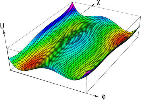
Figure 1: The scalar potential in the model considered in Sect. 3.2.

The theory has two symmetry breaking minima. When both coupling constants $\lambda,\zeta$ are large, those are

$$\{\phi=\eta,\ \ \ \chi=\mu\}\,\,\,\mbox{and}\,\,\,\{\phi=-\eta,\ \ \ \chi=-\mu\}\,.$$ (30)

Let us now derive an effective potential for the field $\chi$ by integrating out $\phi$. To calculate the effective potential in the leading adiabatic approximation we fix the value of $\chi$ and solve for $\phi$ in this background. Note that for a fixed and not too large value of $\chi$ the potential for $\phi$ has two local minima. Generically, the two local minima are nondegenerate. For $\chi<0$ the state $\phi=-\eta$ has lower energy , while for $\chi>0$ the global minimum is at $\phi=\eta$. At $\chi=0$ both local minima become degenerate. At this point there is a discontinuous change of the vacuum in the heavy sector. As a result the effective potential develops a cusp of precisely the same nature as discussed in the previous section,

$$U_{\rm eff}=-\kappa^{2}\eta|\chi|+\frac{\zeta}{2}(\chi^{2}-\mu^{2})^{2}\,.$$ (31)

Thus, although the underlying theory is perfectly smooth, the effective theory has two sectors and a cusp at $\chi=0$ (Fig. 2).

Figure 2: The effective potential obtained after the heavy field $\phi$ is integrated out. The cusp at $\chi=0$ reflects a restructuring of the vacua in the $\phi$ sector.

We can again pose the question about the existence of the wall, and the calculability of its energy density from the effective Lagrangian. Clearly there exists a solution of the original equations of motion, stemming from Eq. (29), with the wall boundary conditions, i.e. interpolating between the two vacua of Eq. (30). It is equally clear that the estimate of its energy from the effective Lagrangian will be generically incorrect. The obvious reason is that the effective Lagrangian is completely independent of the larger mass scale $M$. This is natural since it was calculated in the leading adiabatic approximation, i.e. in the limit $M\rightarrow\infty$. On the other hand, to produce the wall one has to excite the heavy field $\phi$, which jumps from $-\eta$ to $+\eta$ inside the wall profile. This costs energy proportional to $M$, so the wall energy density in this theory must be proportional to $M$. The wall tension in the present example can be calculated directly from the “fundamental” Lagrangian (29) without appealing to the effective Lagrangian (31). Roughly it behaves as

$$\varepsilon=xM\eta^{2}+ym\mu^{2}$$ (32)

where $x$ and $y$ are numbers of order one. If the expectation values of the heavy and light fields are of the same order, $\eta\sim\mu$, the bulk of the wall energy is contributed by the heavy modes. In that case the wall energy can not be obtained from the effective potential for $\chi$. One can say that a dominant part of the wall tension is associated with the cusp.

Physically the picture of what is happening is very simple. The field $\chi$ is light and therefore changes slowly inside the wall, on the scale $1/m$. The heavy field $\phi$ follows this change adiabatically almost everywhere in space, except for the region where $\chi=0$. In this region, within a distance of order $1/M$, the value of $\phi$ changes from $-\eta$ to $\eta$. The big contribution to the wall energy density, proportional to $M$ comes precisely from this small region in space in which the field $\chi$ sits on the cusp of the effective potential.

If we use the effective potential to calculate the wall energy, the result will be of order $m\mu^{2}$, since this is indeed the contribution of the light field. The contribution of the heavy fields can be thought of as an extra contribution of the cusp in the light field effective potential.

There are several lessons we want to draw from this toy model. First, the physical reason for the appearance of the cusp in the effective potential (glued potential) at some value $\chi_{0}$ of the field is that at this particular value of the light field, the system of heavy fields has two (or more) degenerate ground states. In general, when the value of the light field changes continuously, the heavy fields follow adiabatically after this change. However when the light field passes through $\chi_{0}$, there is a level crossing in the heavy system and the properties of the heavy field vacuum change discontinuously. This “first order phase transition” leads to discontinuity in the first derivative of the effective potential, and, therefore, a cusp.

The second lesson, is that the wall configuration that connects the points on different sides of the cusp necessarily involves excitation of heavy modes. This is so since close to the point $\chi_{0}$ inside the wall the heavy modes must rearrange in order to make the transition between the two degenerate vacuum states.

Finally, the description of the wall with the help of naive glued potential is not valid if the bulk of the wall energy comes from the change of the heavy fields. The problem stems from the fact that the effective potential is calculated in expansion in powers of $1/M$, which is the adiabatic approximation. As we already stressed, the adiabatic approximation breaks down inside the wall due to the level crossing. On one hand, this is a signal of possible appearance of terms proportional $M$ in the effective action. On the other hand, this is precisely the situation in which a nontrivial topological Berry phase should appear. A more careful calculation of effective action should reveal the presence of the terms of the type

$$M[\phi(\infty)-\phi(-\infty)]^{2}\,.$$ (33)

This topological term does not affect the vacuum sector, but adds the missing large piece, cusp contribution to the energy of the wall.

Returning to SUSY gluodynamics it is now clear why the original BPS bound is so badly violated by a wall configurations in the effective theory. The reason is that the effective theory misses a large cusp contribution to the energy which comes from the heavy modes not appearing in the effective Lagrangian that are excited inside the wall. We conclude, therefore, that the Veneziano–Yankielowicz effective Lagrangian, as it stands, can not be used to calculate the wall energy; without additional information we can not say whether or not the BPS saturated type II walls exist in SUSY gluodynamics.

In the next section we would like to give a detailed example of how this situation arises in a supersymmetric theory. The model we will consider has the same symmetries as SUSY gluodynamics and an effective potential of the Veneziano–Yankielowicz type. We will see in detail how the cusp structure of the effective Lagrangian appears when integrating out the heavy superfields and will be able to trace exactly the missing piece of the wall energy.

3.3 Supersymmetric model with $N$ sector superpotential

The model of the previous subsection was only intended for explaining how cusps arise in the effective potential. We now want to consider a model which captures more features inherent to SUSY gluodynamics. Consider a generalized Wess-Zumino model of two scalar chiral superfields $\Phi$ and $X$, with the superpotential

$${\cal W}={a\over N+2}\Phi^{N+2}-b\Phi X+{c\over 2}X^{2}\,,$$ (34)

where the coefficients $a,b$ and $c$ are real positive numbers. This model obviously has a $Z_{N}$ symmetry, under which

$$\Phi\rightarrow\Phi e^{i{2\pi n/N}}\,,\,\,\,X\rightarrow Xe^{i{2\pi n/N}}\,,\,\,\,\theta\rightarrow\theta e^{i{2\pi n/N}}\,.$$ (35)

The global minima of the energy are determined from the equations

$${\partial{\cal W}\over\partial\Phi}=a\Phi^{N+1}-bX=0\,,\,\,\,{\partial{\cal W}\over\partial X}=-b\Phi+cX=0\,.$$ (36)

These equations have one $Z_{N}$ symmetric solution

$$\Phi=X=0$$ (37)

and $N$ solutions which spontaneously break the $Z_{N}$ symmetry

$$\Phi_{n}=\left({b^{2}\over ac}\right)^{1/N}e^{i{2\pi n/N}},\ \ \ \ \ X_{n}={b\over c}\,\Phi_{n}\,.$$ (38)

Choosing $b\gg c$, we find that the field $\Phi$ near the asymmetric vacua is very heavy; its mass

$$M=(N+1)\,{b^{2}\over c}\,,$$ (39)

while the field $X$ is light, with the mass $m=c$ .

The effective potential for the field $X$ is obtained by eliminating the heavy field $\Phi$ by virtue $\partial{\cal W}/\partial\Phi=0$, see the first equation in (36). The condition $\partial{\cal W}/\partial\Phi=0$ has $N+1$ solutions

$$\Phi_{*}(X)=\left({b\over a}X\right)^{1\over N+1}\exp\left\{{2\pi in\over N+1}\right\}\,.$$ (40)

The solution has to be substituted in the superpotential,

$${\cal W}[\Phi,X]\rightarrow{\cal W}[\Phi_{*}(X),X]=$$

$$-\frac{N+1}{N+2}b\left(\frac{b}{a}\right)^{1/(N+1)}X^{(N+2)/(N+1)}\exp\left(\frac{2\pi in}{N+1}\right)+\frac{c}{2}X^{2}\,.$$ (41)

This is not the end of the story, however. The effective superpotential is obtained by choosing for every value of $X$ the solution that gives a minimal energy. The energy as a function of the lowest component $\chi$ of the superfield $X$ for each branch is

$$\left|-b\left({b\over a}\chi\right)^{1\over N+1}\exp\left\{{2\pi in\over N+1}\right\}+c\chi\right|^{2}\,.$$ (42)

Clearly, the energy is minimal for the branch for which Arg$\chi$ is closest to

$${2\pi n\over N+1}+{1\over N+1}{\rm Arg}\,\chi\,.$$

For instance, if $\chi$ is real and positive, $n=0$, if Arg$\chi=2\pi/N$ then $n=1$, and so on. At Arg$\chi=\pi/N$ both branches, with $n=0$ and $n=1$, have the same energies. The resulting effective superpotential has $N$ sectors and is “glued” along $N$ rays,

$${\cal W}_{\rm eff}={c\over 2}X^{2}-{N+1\over N+2}\,b\left({b\over a}\right)^{1\over N+1}X^{{(N+2)}/{(N+1)}}\,,$$ (43)

$$\mbox{at}\,\,\,-{\pi\over N}<{\rm Arg}\chi<{\pi\over N}\,,$$

$${\cal W}_{\rm eff}={c\over 2}X^{2}-{N+1\over N+2}\,b\left({b\over a}\right)^{1\over N+1}\exp\left\{{2\pi i\over N+1}\right\}X^{{(N+2)}/{(N+1)}}\,,$$ (44)

$$\mbox{at}\,\,\,{\pi\over N}<{\rm Arg}\chi<{3\pi\over N}\,,$$

and so on (see Eq. (41)). The discontinuities in the effective superpotential (or, equivalently, the cusps in the effective potential) occur along the rays

$${\rm Arg}\chi=\frac{(2k+1)\pi}{N}$$

where two branches in Eq. (40) with $n=k$ and $n=k+1$ are degenerate in energy, see Eq. (42). For instance, at Arg$\chi=\pi/N$

$${\cal W}_{\rm eff}(\chi_{\wedge\pm})=e^{2\pi i/N}\left[\frac{c|\chi|^{2}}{2}-\frac{N+1}{N+2}b\,\left(\frac{b}{a}\right)^{\frac{1}{N+1}}|\chi|^{(N+2)/(N+1)}\exp\left(\pm\frac{\pi i}{N+1}\right)\right]\,.$$

Now we are ready to address the issue of the domain walls. Consider a domain wall that connects two adjacent asymmetric vacua. The BPS bound on its tension is

$$\varepsilon>2|{\cal W}(\Phi_{0},X_{0})-{\cal W}(\Phi_{1},X_{1})|={2N\over N+2}{b^{2}\over c}\left({b^{2}\over ac}\right)^{2\over N}\,\sin\left({2\pi\over N}\right)\,.$$ (45)

At large $N$ this is of order $1/N$. On the other hand, a naive estimate based on the effective potential for the light field would yield

$$\varepsilon\sim m\left|\Delta\chi\right|^{2}\sim{b^{2}\over c}\left({b^{2}\over ac}\right)^{2\over N}\,\frac{1}{N^{2}}\sim N^{-2}\,.$$ (46)

Just like in SUSY gluodynamics the two expressions are incompatible. We know already that the reason is that the adiabatic approximation used to derive the effective Lagrangian breaks down at the cusp. For configurations crossing the cusp an extra “topological” term has to be added to the effective Lagrangian, as discussed in the previous section. Let us first estimate a part of the tension associated with the cusp, and the corresponding restructuring of the heavy field $\phi$. A straightforward estimate analogous to that of Eq. (46) is

$$\varepsilon_{\wedge}\sim M|\Delta\phi|^{2}\sim{b^{2}\over c}\left({b^{2}\over ac}\right)^{2\over N}\,\frac{1}{N}\,,$$ (47)

i.e. we reproduce the order of magnitude of the BPS bound (45).

As a matter of fact, in the present case one can do better than that. To this end we note, that the only point where the adiabatic approximation breaks down is at the cusp. In other words, almost everywhere throughout the space the heavy field $\phi$ does indeed follow the change of $\chi$ adiabatically. Only at the point inside the wall, where

$$\chi=\rho e^{i\pi/N}\,,$$

the value of $\phi$ changes rapidly. This change, of course, does not happen abruptly, but rather on the scale of the inverse mass $M^{-1}$ of the field $\phi$. The field $\chi$ remains constant throughout the region of space where the rapid variation of $\phi$ takes place. The profile of $\phi$ in this region as well as the energy associated with this variation can be calculated by considering the original theory at a frozen cusp value of $\chi$.

If $\chi=\rho\exp{(i\pi/N)}$, the wall profile of the field $\phi$ is determined from the following superpotential

$${\cal W}_{\phi}={a\over N+2}\Phi^{N+2}-b\rho e^{i\pi/N}\Phi\,.$$ (48)

At $\chi=\rho\exp{(i\pi/N)}$ the two branches of Eq. (40) are degenerate. The $\phi$ wall under consideration interpolates between

$$\phi_{*0,1}=\left({b\over a}\rho\right)^{1\over N+1}\,\exp\left[i\pi\left(\frac{1}{N}\pm\frac{1}{N+1}\right)\right]\,,$$ (49)

where the upper and lower signs correspond to the final and initial points, respectively. These points are two degenerate minima of the potential stemming from Eq. (48). The $\phi$ wall in question is BPS saturated. This is because the BPS equation in this case is a pair of the first order equations for two real fields (real and imaginary parts of $\phi$),

$$\partial_{z}\phi=\frac{d\bar{{\cal W}}}{d\bar{\phi}}\,\exp\left(-\frac{i\pi}{2}+\frac{2\pi i}{N}\right)\,,$$ (50)

which possess one conserved quantity (see Ref. [4] for details)

$${\rm Im}\,\left[({\cal W}(\Phi)-{\cal W}(\Phi_{*0}))\exp\left(\frac{i\pi}{2}-\frac{2\pi i}{N}\right)\right]\,=0\,.$$ (51)

Using Eq. (51) one can always eliminate one real field, getting in this way a trajectory in the plane $\{\mbox{Re}\phi\,,\,\mbox{Im }\phi\}$ that connects $\phi_{*0,1}$. The trajectory depends on one real variable. The resulting one first-order equation for one real function always has a solution.

We conclude that the tension of the $\phi$ wall (the cusp term) is given by the BPS bound for the theory with the superpotential (48),

$$\varepsilon_{\wedge}=4\,{N+1\over N+2}\,(b\rho)^{(N+2)/(N+1)}a^{-{1/(N+1)}}\sin{\pi\over N+1}\,.$$ (52)

This is precisely the term that has to be added to the effective potential of $\chi$ in order to be able to calculate the wall tension properly. Equation (52) can be generalized to a wall configuration which connects any two vacua, and not necessarily the two adjacent ones. The extra term in this case would be just the sum of contributions of all cusps crossed by the wall.

Note that although the $\phi$ component is built above through the BPS saturation, the full $\{\phi\,,\,\chi\}$ wall in the original theory is not BPS-saturated, at least, in some range of parameters. (We mean the type II wall connecting, say, two neighboring asymmetric vacua with $n=0$ and $n=1$ in Eq. (38).)

To see that this is indeed the case consider the model (34) with $a=b=c=1$ and $N\gg 1$. (For these values of parameters the field $\Phi$ is still much heavier than $X$, see the footnote following Eq. (39)). Assume that the wall is BPS saturated. Then

$$\partial_{z}\phi=\left(\bar{\phi}^{N+1}-\bar{\chi}\right)\,\exp\left(\frac{i\pi}{2}+\frac{2i\pi}{N}\right)\,,\,\,\,\partial_{z}\chi=\left(-\bar{\phi}+\bar{\chi}\right)\,\exp\left(\frac{i\pi}{2}+\frac{2i\pi}{N}\right)\,.$$ (53)

As a consequence,

$$\partial_{z}\phi+\partial_{z}\chi=\left(\bar{\phi}^{N+1}-\bar{\phi}\right)\,\exp\left(\frac{i\pi}{2}+\frac{2i\pi}{N}\right)\,,$$ (54)

where the right-hand side contains no dependence on $\bar{\chi}$. We can take advantage of this fact. Multiply both sides by $\partial_{z}\bar{\phi}$ and integrate over $z$ from $-\infty$ to $+\infty$. Then

$$\int_{-\infty}^{\infty}(\partial_{z}\phi+\partial_{z}\chi)\partial_{z}\bar{\phi}dz=\exp\left(\frac{i\pi}{2}+\frac{2i\pi}{N}\right)\,\left[\frac{1}{N+2}{\bar{\phi}}^{N+2}-\frac{1}{2}{\bar{\phi}}^{2}\right]_{-\infty}^{\infty}=-\frac{\varepsilon_{\rm BPS}}{2}\,,$$ (55)

where $\varepsilon_{\rm BPS}$ is the tension defined on the right-hand side of Eq. (45) and the values of the $\phi$ field in the vacua, Eq. (38), are substituted. Equation (55) implies

$$\int_{-\infty}^{\infty}(\partial_{z}\chi)(\partial_{z}\bar{\phi})dz=-\frac{\varepsilon_{\rm BPS}}{2}-C_{1}$$ (56)

where $C_{1}$ is a real positive number. On the other hand,

$$C_{2}=\int_{-\infty}^{\infty}(\partial_{z}\phi+\partial_{z}\chi)(\partial_{z}\bar{\phi}+\partial_{z}\bar{\chi})dz=\int_{-\infty}^{\infty}(\partial_{z}\phi\partial_{z}\bar{\phi}+\partial_{z}\chi\partial_{z}\bar{\chi})+$$

$$\left[\int_{-\infty}^{\infty}(\partial_{z}\chi)(\partial_{z}\bar{\phi})dz+\mbox{H.c.}\right]$$ (57)

where $C_{2}$ is a real positive number. The first term is obviously equal to $\varepsilon_{\rm BPS}/2$, while the second term can be read off from Eq. (56). In this way we obtain

$$C_{2}=\frac{\varepsilon_{\rm BPS}}{2}+2\left(-\frac{\varepsilon_{\rm BPS}}{2}-C_{1}\right)\,,$$ (58)

or $C_{2}+2C_{1}=-\varepsilon_{\rm BPS}/2$. This relation is obviously inconsistent, which proves that we cannot built a BPS saturated wall in the problem at hand.

Thus, the lesson to be drawn is as follows. Consideration of the effective low-energy theory, by itself, yields information on the vacuum structure. The fact of existence of the walls can be unambiguously inferred from this information. But neither the nature of the wall (BPS versus non-BPS), nor its tension can be properly found from the analysis of the effective low-energy theory if the corresponding potential is glued from distinct sectors, and the wall in question crosses the cusps.

3.4 Elements of the general theory

Given an effective low-energy theory, obtained after integrating out all heavy fields, with a discrete set of degenerate vacua (as it is typical for supersymmetry), the question we ask is: can one infer from this low-energy theory the existence of the BPS walls interpolating between the distinct vacua? Under what circumstances the BPS wall seen in the effective theory is a reflection of the wall in the full theory? And vice versa, if we see no BPS walls in the effective low-energy theory does it mean there are no such walls in the full theory?

The full general theory is not yet worked out, and the answers to these questions in the generic situation are not known so far. In this section we will present some illustrative considerations which are valid in the simplest possible setting: the generalized Wess-Zumino models, with all parameters in the superpotentials that are real. We will limit ourselves to the wall solutions where all fields take real values, so we do not have to travel in the complex plane, and can apply a rich physical intuition stemming from the fact that the BPS equations in this case are those of high-viscosity fluid (the so called creek equations) [4]. We will see that even in this simplest case the situation is quite non-trivial. Whenever the low-energy theory has a glued potential, we can count the number of distinct walls but, generically, can say nothing about their BPS nature and/or tension.

Let us consider for simplicity two chiral superfields, $\Phi$ and $X$, and a superpotential shown on Fig. 3. (More exactly, Fig. 3 displays ${\cal W}$ as a function of $\phi,\chi$ for real values of $\phi,\chi$.) Shown are two “mountain ridges”, the left ridge and the right one, separated by a “canyon”. The heavy field is $\Phi$, the light one is $X$. The vacua of the theory correspond to the points where

$$\frac{\partial{\cal W}}{\partial\Phi}=0\,,\,\,\,\frac{\partial{\cal W}}{\partial X}=0\,.$$ (59)

These points are denoted by $A,B,C,D,E$ on Fig. 4. The points $A,B,C$ lie on the left ridge, the point $D$ on the right ridge while the point $E$ belongs to the bottom of the canyon.

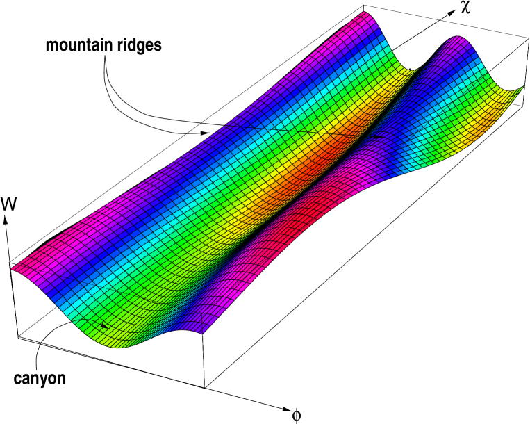
Figure 3: A superpotential with two mountain ridges and a canyon and five vacuum states.

Figure 4: The projection of the superpotential of Fig. 3 onto the ${\cal W}\chi$ plane. Shown are the shapes of the mountain ridges and the canyon bottom. The points of extrema in ${\cal W}$ are denoted by $A,B,C,D,E$.

The low-energy reduction is obtained by eliminating the field $\Phi$ by virtue of the equation

$$\frac{\partial{\cal W}(\Phi,X)}{\partial\Phi}=0\,\,\,\rightarrow\,\,\,\Phi=\Phi_{*}(X)\,.$$ (60)

Substituting $\Phi_{*}(X)$ back in the superpotential ${\cal W}$ we get an effective low-energy superpotential

$${\cal W}_{\rm eff}(X)={\cal W}(\Phi_{*}(X),X)\,.$$ (61)

Equation (60) determines the positions of the mountain ridges and the bottom of the canyon, while Eq. (61) projects them onto the ${\cal W}\chi$ plane. One can visualize ${\cal W}_{\rm eff}$ as shadows of the ridges left by a parallel horizontal beam of light in the $\phi$ direction.

First of all, let us prove that the vacua of the full theory (extrema of ${\cal W}$) lie on the mountain ridges and/or bottoms of the canyons (extrema of ${\cal W}_{\rm eff}$ ). Indeed,

$$\frac{d{\cal W}_{\rm eff}}{dX}=\left[\frac{\partial{\cal W}(\Phi,X)}{\partial X}+\frac{\partial{\cal W}(\Phi,X)}{\partial\Phi}\,\frac{\partial\Phi_{*}}{\partial X}\right]_{\Phi=\Phi_{*}(X)}=0\,,$$

if Eq. (59) is satisfied. Thus, the extrema of ${\cal W}_{\rm eff}$ and ${\cal W}$ coincide.

Let us assume now, for a short while, that the right mountain ridge and the canyon do not exist, and the profile of ${\cal W}$ has only the left mountain ridge, with three vacua, $A,B$ and $C$. In this case the solution of Eq. (60) is unique. The full theory has two BPS walls: $AB$ and $CB$. The potential of the low-energy effective theory ${\cal W}_{\rm eff}(X)$ is a smooth function, and the low-energy theory has two BPS walls too. Their existence can be seen from the creek equation in the low-energy theory per se,

$$\partial_{z}X=\frac{d{\cal W}_{\rm eff}}{dX}\,.$$ (62)

The wall profile $X(z)$ we find from Eq. (62) is a little bit different from what one would get by solving the creek equations in the full theory,

$$\partial_{z}X=\frac{\partial{\cal W}(\Phi,X)}{\partial X}\,,\,\,\,\partial_{z}\Phi=\frac{\partial{\cal W}(\Phi,X)}{\partial\Phi}\,.$$ (63)

The difference vanishes in the limit when the field $\Phi$ becomes infinitely heavy; it dies off as positive powers of $1/M_{\phi}$. At the same time , the wall tension found in the effective theory exactly coincides with that one would find in the full theory. No $1/M_{\phi}$ corrections can appear. This is a remarkable feature of BPS supersymmetric walls. The tension of such a wall is exactly determined by the central charge [3, 4, 7] which reduces, in turn, to $|{\cal W}(\Phi_{0},X_{0})-{\cal W}(\Phi_{1},X_{1})|$ in the full theory, and to $|{\cal W}(X_{0})_{\rm eff}-{\cal W}(X_{1})_{\rm eff}|$ in the effective low-energy theory. (Here $\{\Phi_{0,1},X_{0,1}\}$ are the points of extrema.) The two expressions above coincide identically.

Summarizing, if for all values of the light fields the solution for the heavy fields, to be integrated out, is unique, the existence of a BPS wall in the effective theory entails the existence of such a wall in the full theory, and vice versa. Moreover, if one calculates the wall tension in the effective theory, one gets the exact answer valid in the full theory, with no $1/M_{\phi}$ corrections.

Let us return to the superpotential depicted on Fig. 3, with two mountain ridges and one canyon. In addition to the $AB$ and $CB$ walls, the full theory has a $BE$ wall which is BPS saturated, and three continuous sets of BPS walls $AE$, $CE$ and $DE$. Each set includes an infinite amount of degenerate walls (by degenerate we mean that the tensions of all walls inside each set are the same). The phenomenon of continuously degenerate supersymmetric walls was first observed in Ref. [25]. Besides these BPS walls, the full theory may have $AD,BD$ and $CD$ walls that are not BPS saturated. Depending on the values of parameters in the superpotential it may be expedient for some or all non-BPS walls to decay into a pair of BPS walls.

What can be said about the effective theory? The corresponding low-energy effective potential will be glued out of five pieces, as indicated in Fig. 4. In each of five domains, the branch of the effective superpotential corresponding to the lowest energy is shown by rectangles. We get a typical five-sector structure of the scalar potential in the effective theory. ¿From this structure we conclude, with certainty, that the theory under consideration has five degenerate vacuum states, so that each pair can be connected by a domain wall. Inspecting the low-energy theory, without additional information on the full theory, we can say nothing, generally speaking, as to the nature of these walls. The reason is obvious: we have no idea where each sector comes from, whether or not two extrema in question belong to one and the same mountain ridge (canyon). If they do, no restructuring of the heavy field $\phi$ vacuum occurs inside the wall, and we return back to the situation with the unique solution of Eq. (60) discussed above.

If extrema from different sectors actually do belong to distinct mountain ridges or canyons (Eq. (60) has more than one solution) there is no unambiguous way to decide BPS versus non-BPS from inspection of the low-energy theory alone. We need additional information regarding what happens with the heavy fields inside the wall. In any case, a part of the wall tension associated with the light fields will not saturate $\varepsilon$.

4 The Kaluza-Klein Domain Wall

As was discussed above, the tension of the walls interpolating between the neighboring vacua in supersymmetric gluodynamics is expected to scale as $N$ rather than $N^{2}$. This gives rise to a natural identification of these walls with the $D$-brane solutions found in Ref. [9]. Here we will show, that this phenomenon, “abnormal” $N$ dependence, is actually more general, and shows up in other wall configurations related to Witten’s analysis. In fact, the low-energy limit of the theory considered in Ref. [9] is a five-dimensional Kaluza-Klein (KK) theory with a five-dimensional $SU(N)$ gauge field $A_{M},~{}M=1,..,5$ and charged matter. After compactification there are two types of gauge fields – our original $SU(N)$ gauge field $A_{\mu}$ and a new $U(1)$ gauge field $B_{\mu}$ coming from the $G_{\mu 5}$ components of the metric tensor as well as a scalar made from the fifth component $A_{5}$ of the $SU(N)$ gauge field. We are going to demonstrate that if this theory is modified, so that the supersymmetry is broken explicitly, there is a new type of domain wall due to the field $A_{5}$. By analyzing this low-energy theory per se, with no reference to $D$-branes, we demonstrate that the wall tension scales as $N$, in parallel with the brane-based derivation of Ref. [9]. Moreover, these walls carry an induced fractional charge [18]. Conceptually the situation reminds that with the axion wall discussed in Sect. 2.2.

The theory to be considered is gravity plus the gauge field $A_{M}$ in five dimensions. To warm up we start from the Abelian case, i.e. the $U(1)$ gauge group. At this stage we also omit the superpartners from the discussion. The action is

$$S=\int d^{5}x\sqrt{-G}\left[-\kappa_{5}R-\frac{1}{4e^{2}_{5}}F_{MN}F^{MN}+G^{MN}(\partial_{M}-iA_{M})\Phi^{\ast}(\partial_{N}+iA_{N})\Phi\right],$$ (64)

where $\kappa_{5}$ and $e_{5}$ are the five-dimensional gravitational and gauge coupling constants, $G_{MN}$ is the metric, $R$ stands for the curvature, $F^{MN}$ is the gauge field strength tensor, all capital Latin letters run from 1 to 5, say, $M,N=1,...,5$, while the Greek letters $\mu,\nu\,,...=1,...,4$. It is assumed that one of the five dimensions forms a circle, so that we deal with $M^{4}\times S^{1}$ KK model. The mater sector consists of charged scalars $\Phi$, the simplest possible choice.

After $M^{4}\times S^{1}$ decomposition of the metric

$$G_{MN}=\left(\begin{array}[]{lc}g_{\mu\nu}&B_{\mu}\\ B_{\nu}&1+B_{\mu}B^{\mu}\end{array}\right);\;G^{MN}=\left(\begin{array}[]{lc}g^{\mu\nu}+B^{\mu}B^{\nu}&-B^{\mu}\\ -B^{\nu}&1\end{array}\right)$$ (69)

we get four-dimensional gravity, two $U(1)$ gauge fields $A_{\mu}$ and $B_{\mu}$, plus a scalar $A_{5}$ (we put dilaton $G^{55}=1$).

For any manifold $K$ with a nontrivial $\pi_{1}(K)$ the KK theory contains special Wilson line operators

$$U_{\gamma}=P\,exp\,\left(i\oint_{\gamma}Adx\right)\,,$$ (70)

where $\gamma$ is a closed noncontractible contour on $K$. In our case $K=M^{4}\times S^{1}$ and $\pi_{1}(S^{1})=Z$. For the $U(1)$ gauge field

$$U=e^{i\phi},\;\;\;\;\phi\in[0,2\pi)\,.$$

The phase $\phi$ represents the constant component of the gauge field $A_{5}=[0,1/R]$, where $R$ is the compactification radius. Other values of $A_{5}$ can be gauged into the interval $[0,1/R)$ while $A_{5}=1/R$ is gauge equivalent to $A_{5}=0$. The corresponding gauge function is $\epsilon=x_{5}/R$. This means that the charged (with respect to field $A$) fields are related by a gauge transformation,

$$\Psi_{A_{5}=1/R}(x,x_{5})=e^{ix_{5}/R}\Psi_{A_{5}=0}(x,x_{5})$$ (71)

where $x$ denotes four noncompact coordinates. Using the standard KK decomposition

$$\Psi(x,x_{5})=\sum_{n=-\infty}^{\infty}e^{inx_{5}/R}\Psi_{n}(x)\,,$$ (72)

where $\Psi_{n}(x)$ describes different four-dimensional fields with masses $m^{2}_{n}=n^{2}/R^{2}$ and charges $q=n$ with respect to the KK gauge field $B_{\mu}=G_{\mu 5}$, we see that the gauge transformation (71) shifts $n\rightarrow n+1$:

$$\Psi_{n}(x)|_{A_{5}=1/R}=\Psi_{n+1}(x)|_{A_{5}=0}$$ (73)

Changing adiabatically $A_{5}$ from zero to $1/R$ all levels in the particle spectrum are shifted by one. For example, a massless neutral (with respect to $B_{\mu}$) particle will be transmuted into a heavy ($m=1/R$) charged ($q=1$) particle. Thus, if there is a domain wall $A_{5}(x)$ interpolating between $A_{5}(-\infty)=0$ and $A_{5}(\infty)=1/R$, and one scatters a massless neutral particle with $n=0$ on the domain wall it either reflects or becomes massive and charged. The total KK charge must be conserved in the process, since it is the gauge charge which generates a part of the general coordinate transformation, $\delta G_{MN}=\partial_{M}\epsilon_{N}(x,x_{5})+\partial_{N}\epsilon_{M}(x,x_{5})\,$ which for $\epsilon_{M}(x,x_{5})=\delta_{M,5}\epsilon(x)$ is the $U(1)$ gauge transformation, $\delta B_{\mu}=\delta G_{\mu 5}=\partial_{\mu}\epsilon$.

The conservation of the KK charge is insured in a way very similar to the one discussed in Sect. 2.2. In the presence of the charged particles the domain wall itself acquires an induced KK charge $q$. The total charge of the domain wall plus the particle is conserved. The real process of the particle penetration through the domain wall looks as follows: the initial state is the KK neutral particle($q=n=0$) plus the charged domain wall, with the charge $q_{i}=+1/2$. The final state (if the particle initially has momentum $p_{x}>1/R$) is the charged particle $q=n=1$ plus the domain wall with the charge $q_{f}=-1/2$. The total charge $+1/2$ is conserved.

These walls have a variety of interesting properties. Thus, for example, if the theory contains fermions, their charge may be half integer. In this case the charges of the wall and the fermion are exchanged in the scattering process and there is no threshold energy for this process. Moreover the fermion and the wall can form a neutral bound state. For a detailed discussion see Ref. [18].

Under what circumstances is this wall stable? The five-dimensional Maxwell term $(1/4e_{5}^{2})F_{MN}^{2}$ gives rise to the four-dimensional kinetic term $(1/4e^{2})\partial_{\mu}A_{5}\partial_{\mu}A_{5}$ where $e$ is the four-dimensional gauge coupling. It is quite evident that to get a stable domain wall an effective potential (which does not exist at the classical level) must be generated. Such an effective potential $U(A_{5})$ is indeed induced at the one-loop level. The mass operator for the scalar field modes is

$$\hat{m}=-i\partial_{5}+A_{5};\;\;\;\;m_{n}=\frac{n}{R}+A_{5}\,.$$ (74)

The mass spectrum depends on the value of $A_{5}$ with periodicity $1/R$. Due to this dependence there is an effective potential for the field $A_{5}$ which is given, at one loop, by (see [26] for details)

$$V(A_{5})=\frac{1}{(2\pi R)^{4}16\pi^{2}}\int dtt^{3}\ln(1-2e^{-t}\cos 2\pi RA_{5}+e^{-2t})\,.$$ (75)

This potential is periodic in $A_{5}$, with the period $1/R$. It has minima at $A_{5}=n/R$. Using this effective potential it is not difficult to see that the wall width $L$ is of the order of $R/e$ and the energy density (wall tension) scales as

$$L(1/e^{2})(1/RL)^{2}=(1/e)(1/R^{3}).$$

Observe that the wall tension scales as $1/e$ rather than $1/e^{2}$. This is essentially the same difference as between the $N$ and $N^{2}$ scaling laws in SUSY gluodynamics. Indeed, $1/N$ is an effective coupling constant in the string description of the gauge theory.

The same $N$ dependence arises also in the non-Abelian case. If there are no fields transforming in the fundamental representation, the gauge group $G$ is actually not $SU(N)$ but $SU(N)/Z_{N}$ and $\pi_{1}(G)=Z_{N}$, so one may have a $Z_{N}$ domain wall. The domain walls will be somewhat more complicated: instead of one phase field there are $N-1$ independent phases (=rank of the group $SU(N)$).

In the supersymmetric theory the situation is essentially different. The fermions and the bosons give contributions of the opposite signs to the effective potential, which, thus, cancel each other. This is so since supersymmetry should be maintained at any value of $A_{5}$ and the vacuum energy must be zero. Therefore, in five-dimensional SUSY gauge theory (which is essentially a low-energy limit of Witten’s theory) there are no stable domain walls of the type just discussed. To get a non-zero one-loop effective potential supersymmetry must be broken explicitly. This can be achieved either by imposing different boundary conditions on bosons and fermions, or by adding non-SUSY mass terms by hand, or in any other way – in any case there will be an induced effective potential. In the particular case of $M^{4}\times U(1)$ relevant details can be found in Ref. [26], and the result for the wall tension in the large $N$ limit is

$$\varepsilon\sim\frac{N}{R^{3}}\frac{1}{e\sqrt{N}}\,.$$ (76)

At large $N$ the proper coupling constant is not $e$ but $g=e\sqrt{N}$, and the domain wall tension has a typical $D$-brane behavior – linear in both $N$ and $1/g$,

$$\varepsilon\sim(N/g)(1/R^{3})\,.$$

Thus we see that in the theory of the type considered in [9] (with explicitly broken SUSY) a new type of the domain wall, with an abnormal $N$-dependence, emerges. The $D$-brane interpretation of these walls should also be possible.

5 Comment on Discrete Anomaly Matching

The issue of the discrete anomaly matching in SUSY gluodynamics was raised in Ref. [10], with the conclusion that the chirally symmetric vacuum suggested in Ref. [5] does not satisfy the matching condition, at least in its naive realization. Although this topic is peripheral to the main subject of the present work, we would like to dwell briefly on this issue in view of general important consequences which might follow.

The construction which goes under the name of discrete anomaly matching was suggested in Refs. [28, 29, 30], in a model-building context where it was quite informative and useful. Below we will show that in supersymmetric gluodynamics and similar settings no new physical results can be obtained from the procedure, besides those Ward identities which are already obtained by a different method. These Ward identities neither support nor rule out the chirally symmetric Kovner-Shifman vacuum.

Let us introduce the construction in an explicit form, first in a somewhat simplified setting of a non-supersymmetric Yang-Mills theory, with the intention to revisit SUSY gluodynamics later on. Assume we have a $SU(N)$ Yang-Mills theory with one quark field $\Psi^{a}$ belonging to the adjoint representation of the gauge group. Note that, unlike SUSY gluodynamics, $\Psi$ is the Dirac field, so it can be coupled to an external “electromagnetic” field $A_{\mu}$ vectorially, with a very small coupling constant $e$,

$$\Delta{\cal L}=e\bar{\Psi}^{a}\gamma^{\mu}\Psi^{a}A_{\mu}\,.$$ (77)

The field $A_{\mu}$ is auxiliary and is needed only for the purpose of constructing the ’t Hooft AVV triangles [31]. The quark $\Psi^{a}$ is assumed to be massless.

This theory, classically, has two conserved currents, the vector current $\bar{\Psi}\gamma^{\mu}\Psi$ and the axial one, $\bar{\Psi}\gamma^{\mu}\gamma^{5}\Psi$. (There are two other conserved currents [32], but this is another story.) The vector current is useless from the point of view of the ’t Hooft matching [31] and we will forget about it, focusing on the axial $U(1)$ symmetry associated with the axial current. This symmetry is internally anomalous,

$$\partial^{\mu}\left(\bar{\Psi}\gamma^{\mu}\gamma^{5}\Psi\right)=\frac{N}{8\pi^{2}}G_{\mu\nu}^{a}\tilde{G}_{\mu\nu}^{a}\,,$$ (78)

so that the only remnant of this “non-symmetry” is a discrete $Z_{4N}$. The fact of survival of the discrete $Z_{4N}$ symmetry is most readily seen from the instanton-induced ’t Hooft interaction [33] which in the case at hand includes $4N$ fermion lines. The factor $4N$ is related to the coefficient $N$ in the right-hand side of Eq. (78), which in turn represents $T(G)$, (one half) of the Dynkin index for the adjoint representation. If instead of the adjoint quark we were dealing with the quark in a representation $R$, then $T(G)\rightarrow T(R)$.

The survival of a discrete unbroken subgroup of the axial $U(1)$ is similar to what we have in SUSY gluodynamics.

To construct the ’t Hooft triangles that must be matched at the fundamental and constituent levels we have to have a continuous axial symmetry, rather than a discrete one. The basic idea of the discrete matching [28, 29, 30] is embedding the theory under consideration into a larger one, where we do have a continuous axial symmetry, which is later spontaneously broken down to $Z_{4N}$. The spontaneous breaking should happen in such a way that at low energies we recover the original theory plus possible extra decoupled degrees of freedom. Such an embedding is easy to achieve by exploiting the phantom axion construction [21]. Let us add to our Yang-Mills theory a quark field $Q$ in the fundamental representation of the gauge group. This quark is coupled to a (color-singlet) complex scalar field $\Phi$,

$$\Delta{\cal L}_{\Phi}=h\bar{Q}_{R}Q_{L}\Phi+\mbox{H.c.}+V(|\Phi|)\,,$$ (79)

where $h$ is a coupling constant, and $V(|\Phi|)$ is a self-interaction potential which will eventually ensure the development of a large vacuum expectation value of the field $\Phi$,

$$\langle\Phi\rangle=v\rightarrow\infty\,.$$

When $v$ becomes very large, the quark $Q$ and the modulus of the filed $\Phi$ disappear from the spectrum, leaving only Arg$\Phi$, the axion field, as a remnant. The quark $Q$ and the modulus of the filed $\Phi$ are auxiliary elements of the construction. With the extra fields introduced in this way we have an additional axial $U(1)$ symmetry

$$Q_{L}\rightarrow Q_{L}e^{i\beta}\,,\,\,\,Q_{R}\rightarrow Q_{R}e^{-i\beta}\,,\,\,\,\Phi\rightarrow\Phi e^{-2i\beta}\,.$$ (80)

This symmetry is internally anomalous too. Out of two internally anomalous $U(1)$ symmetries we can readily pick up an anomaly-free combination,

$$\psi_{L}\rightarrow\psi_{L}e^{-i\alpha}\,,\,\,\,Q_{L}\rightarrow Q_{L}e^{-i2N\alpha}\,,\,\,\,\Phi\rightarrow\Phi e^{i4N\alpha}\,.$$ (81)

The corresponding conserved axial current has the form

$$J_{\mu}=\bar{\Psi}\gamma^{\mu}\gamma^{5}\Psi-2N\bar{Q}\gamma^{\mu}\gamma^{5}Q+\mbox{scalar term}\,.$$ (82)

The vacuum expectation value of the field $\Phi$ spontaneously breaks the $U(1)$ symmetry of Eq. (81), but since the corresponding charge of the $\Phi$ field is $4N$, there is a survivor, a $Z_{4N}$ subgroup.

So, we have a theory which, at the fundamental level, has an internally anomaly-free axial $U(1)$ containing a discrete subgroup. At the scale below $v$ only the discrete subgroup survives. Let us examine now implications of the ’t Hooft anomaly matching. The triangle to be considered is AVV where the A vertex is due to the axial current (82), while the vector vertices are due to Eq. (77). Note that the auxiliary quark $Q$ has no coupling to $A_{\mu}$.

The AVV triangle appearing at the fundamental level is

$$\partial^{\mu}J_{\mu}=\frac{N^{2}-1}{8\pi^{2}}F_{\mu\nu}\tilde{F}_{\mu\nu}$$ (83)

where $F_{\mu\nu}$ is the photon field strength tensor built of the auxiliary field $A_{\mu}$. If the photons are on mass shell, Eq. (83) implies [34, 31] the existence of a pole coupled to $J_{\mu}$,

$$\langle J_{\mu}\rangle=\frac{q_{\mu}}{q^{2}}\frac{N^{2}-1}{8\pi^{2}}F_{\mu\nu}\tilde{F}_{\mu\nu}\,.$$ (84)

The coefficient in front of $q_{\mu}/q^{2}$ has to be matched by the contribution of physical massless particles. Some of them may or may not occur dynamically, as composite mesons or baryons built from $\Psi$’s in the original Yang-Mills theory under consideration. More important is the occurrence of the massless axion field, which is coupled to the current $J_{\mu}$ and, thus, participates in the matching with necessity. This is a distinctive feature of the discrete matching, as opposed to the ’t Hooft matching, where such field, totally foreign to the original Yang-Mills theory per se, does not emerge. It is to be stressed that, as opposed to the Peccei–Quinn construction [35], in the present setup the axion is necessarily massless and can not acquire mass through nonperturbative effects. This is so since it is a Goldstone boson appearing due to spontaneous breaking of a continuous global symmetry.

The axion field $a$ is not coupled to the $A_{\mu}$ field because the auxiliary quark $Q$ does not have this coupling. It is coupled, however, to the gluon field, through the standard vertex

$$a\,\frac{1}{32\pi^{2}}\,G_{\mu\nu}^{a}\tilde{G}_{\mu\nu}^{a}\,.$$ (85)

Since its coupling to the current $J_{\mu}$ is

$$J_{\mu}^{\rm axion}=-4Nv^{2}(\partial_{\mu}a)$$ (86)

we conclude that at low energies, in the effective low-energy theory, $\langle J_{\mu}\rangle=\langle J_{\mu}\rangle^{\rm axion}$ plus a possible pole term in $\langle J_{\mu}\rangle$ due to the contribution of massless composites built of $\Psi$, should they exist. Here

$$\langle J_{\mu}\rangle^{\rm axion}=\frac{q_{\mu}}{q^{2}}\left(-\frac{N}{8\pi^{2}}\right)\,\langle 0|G_{\mu\nu}^{a}\tilde{G}_{\mu\nu}^{a}|\gamma\gamma\rangle\,.$$ (87)

The momentum $q$ in Eq. (87) is the momentum flowing in the $G\tilde{G}$ vertex (the total momentum of the photon pair). It is assumed that $q\rightarrow 0$.

The matching of Eqs. (84) and (87) tells us that

$$\frac{N^{2}-1}{8\pi^{2}}F_{\mu\nu}\tilde{F}_{\mu\nu}+\left(\frac{N}{8\pi^{2}}\right)\,\langle 0|G_{\mu\nu}^{a}\tilde{G}_{\mu\nu}^{a}|\gamma\gamma\rangle$$ (88)

$$\mbox{= possible contributions due to massless $\Psi$ composites}.$$

If there are none, then the expression on the left-hand side vanishes.

Recall that our initial task was getting information on the emergence or nonemergence of the massless $\Psi$ composites. The entire construction with embedding the discrete remnant of the anomalous axial $U(1)$ was designed for that purpose. We are neither closer nor further now from this goal. Indeed, one can discard this construction altogether, and just consider the internally anomalous current (78). Then, combining both the external and internal anomaly, we would get

$$\partial^{\mu}\left(\bar{\Psi}\gamma^{\mu}\gamma^{5}\Psi\right)=\frac{N}{8\pi^{2}}G_{\mu\nu}^{a}\tilde{G}_{\mu\nu}^{a}+\frac{N^{2}-1}{8\pi^{2}}F_{\mu\nu}\tilde{F}_{\mu\nu}\,.$$ (89)

Sandwiching both sides of this formula between $\langle 0|$ and $|\gamma\gamma\rangle$ in the limit $q\rightarrow 0$ we immediately reproduce Eq. (88). The only interesting dynamical question is whether the left-hand side of Eq. (88) vanishes or not. At first sight the $N$ dependence of two terms in this equation is different, so one is tempted to say that they cannot cancel each other. A closer look shows, however, that the discrepancy is superficial. Indeed, a typical graph for the second term is depicted in Fig. 5. The gluons are converted into photons through the $\Psi$ loop. It is not difficult to count that the matrix element shown in Fig. 5 scales as $N^{2}$, i.e. in the same way as the first term in Eq. (88).

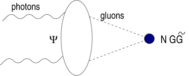
Figure 5: The two-photon matrix element of $NG\tilde{G}$. The photons are assumed to be on mass shell.

If $T(R)$ were a free parameter than one could establish the non-vanishing of Eq. (88) since the second term is proportional to $(T(R))^{2}$ while the first term to dim$R$. The choice of $T(R)$ is not free, however, since, on the one hand, to have a discrete unbroken subgroup $Z_{N}$ we must work with the quarks in representation higher than fundamental, but on the other hand the representation can not be too high, since otherwise we loose asymptotic freedom. For this reason $T(R)$ cannot scale faster than $N$. These two requirements are contradictory unless $T(R)\propto N$.

Thus, Eq. (88) may or may not vanish, depending on whether the two terms cancel each other. As far as the $N$ dependence is concerned, they are perfectly fit to cancel. In the absence of massless composites they would be forced to cancel. This is nothing but the NSVZ low-energy theorem for the two-photon coupling to $G\tilde{G}$ [11].

Instead of the auxiliary photon $A_{\mu}$ we could have considered the coupling to gravitons, i.e. the $U(1)$ current in the gravitational background. Then the issue would reduce to a formula connecting $(N^{2}-1)R\tilde{R}$ to a two-graviton matrix element of $NG\tilde{G}$. Again, the so called discrete matching would have nothing to say whether or not the two terms combine to cancel each other (in the first case there are no massless $\Psi$ composites while in the second they would have to be present to match the anomaly).

Now, we can readily adapt our consideration to SUSY gluodynamics. Again, we could have built a “tower of discrete anomaly matching” by embedding the theory in a larger one where an internally nonanomalous axial $U(1)$ current exists, with the subsequent spontaneous breaking of this $U(1)$ down to $Z_{2N}$, the actual symmetry of SUSY gluodynamics. As we have just demonstrated, this procedure is redundant. It would yield no more constrains or information compared to what one gets considering the axial current of gluinos from the very beginning. The gluino is described by the Majorana field, so we cannot couple it to the auxiliary photon (vector current). However, the anomaly in the gravitational background remains an open possibility. The relation to be analyzed is

$$\partial_{\mu}\left(\bar{\lambda}\gamma^{\mu}\gamma^{5}\lambda\right)=\frac{N}{16\pi^{2}}\langle 0|G_{\mu\nu}^{a}\tilde{G}_{\mu\nu}^{a}|\mbox{2 gravitons}\rangle+\frac{N^{2}-1}{8\pi^{2}}\,C\,R\tilde{R}\,,$$ (90)

where $C$ is a known constant. The question to be answered is: are there massless composites built from gluons/gluinos? In the standard chirally asymmetric phase we expect none, while in the chirally symmetric vacuum of Kovner and Shifman a set of massless composites must exist.

We see that, if at all, the massless composites of the Kovner-Shifman solution facilitate the anomaly matching. Indeed, in the chirally asymmetric vacua the exact cancellation of two terms in Eq. (90) must take place, while in the chirally symmetric one this cancellation can be partial. The missing part will then be filled by the contribution of massless composites. Regardless, the $N$ dependence of both terms in Eq. (90) is the same, and no constraints on the chirally symmetric solution [5] follow.

To summarize, the addition of extra matter which promotes the discrete $Z_{2N}$ symmetry into the continuous one necessarily leads to the appearance of a massless axion. This axion is indeed practically decoupled from the dynamics of the rest of the low energy sector when the symmetry breaking scale $v^{2}$ is large. However, at the same time it couples strongly to the conserved global current by virtue of Eq. (86). As a result, the contribution of the axion to the anomaly matching is finite and independent of the scale $v$. This contribution is the first term on the right hand side of Eqs. (89) and (90). The discrete anomaly matching conditions, therefore, do not pose any restrictions on the spectrum of massless composite fermions but, rather, just determine the contribution of the axion which is not a physical quantity in the original theory. In this language the “modulo $N$” matching of Ref. [10] is the statement that the contribution of the axion to an anomaly triangle has to be an integer multiple of $N$. This statement is true in a simple case when the fundamental fermions acquire mass only due to a Yukawa coupling to the scalar whose vacuum expectation value breaks the global $U(1)$ symmetry down to the discrete subgroup in question. It is, however, not provable as a general result and there is no a priori reason to believe that it holds in strongly interacting theories with confining dynamics, like SUSY gluodynamics.

For example, let us consider the very same toy model (79), but this time, instead of the vector current (77), let us analyze the triangle with two vector currents $\bar{Q}\gamma_{\mu}Q$ (and the same axial current as above). For convenience one can couple $\bar{Q}\gamma_{\mu}Q$ to another auxiliary vector field ${\cal A}_{\mu}$, which is distinct from the field $A$ introduced above. (${\cal A}$ does not couple to $\Psi$.) The gauge strength tensor built from ${\cal A}_{\mu}$ will be denoted by ${\cal F}_{\mu\nu}$. Now we can match the anomaly between the high energy scale $M\gg v$ where the extra quarks $Q$ are massless and the intermediate scale $m$ ($v\gg m\gg\Lambda$). At this scale the quarks $Q$ do not appear in the spectrum anymore. Note that the truly dynamical quarks $\Psi$ and their scale $\Lambda$ are irrelevant in this problem.

In this matching the contribution of the massless axion at the scale $m$ must be equal to the contribution of the fermions $Q$ at the scale $M$, since the only nontrivial dynamics that happens at $v$ is the spontaneous symmetry breaking due to the Higgs field $\Phi$. Since $Q$ couple directly to $\Phi$ their axial charges are necessarily integer multiples of $2N$, Eq. (81). The contribution of $Q$ to the anomalous triangle at $M$ is

$$-4N^{2}\frac{1}{16\pi^{2}}{\cal F}_{\mu\nu}{\tilde{\cal F}}_{\mu\nu}\,;$$

the coefficient is multiple integer of $4N$. Thus, it is indeed true that the contribution of the axion to this anomaly at the intermediate scale $m$ is an integer multiple of $4N$. This is of course trivially so, since the axion coupling

$$a\frac{N}{16\pi^{2}}{\cal F}_{\mu\nu}{\tilde{\cal F}}_{\mu\nu}$$

in conjunction with Eq. (86) automatically guarantee the required proportionality.

We are interested, however, in matching the anomaly between $m$ and a still lower scale $\mu<\Lambda$. We would have the statement about “modulo N” matching here if we knew that the contribution of the axion changes by an integer multiple of $4N$ when crossing the scale $\Lambda$. This we can not know, however, because of the strong nontrivial interaction at $\Lambda$. The best we can do is to express this contribution in terms of a matrix element of $G\tilde{G}$, see Eq.(88). The fact that the axion couples extremely weakly to the gauge field $G$ does not help here, since it is a finite “renormalization” of this weak coupling due the strong interactions of the gauge field and $\Psi$ that determines the contribution of the axion to the anomaly.

6 Discussion

In this paper we have analyzed aspects of the supersymmetric walls in SUSY gluodynamics and in a more general context. We have argued that the linear scaling of the wall tension with $N$ does not contradict the picture where the wall is a classical soliton in an effective Lagrangian describing low-energy mesons and glueballs. We have also provided a simple qualitative explanation of how the confining string can end on a domain wall.

A key part of our analysis is related to the issue what happens when the low-energy Lagrangian has a glued structure. The Veneziano–Yankielowicz description of SUSY gluodynamics belongs to this class.

We have tried to answer the question whether the walls in SUSY gluodynamics are indeed BPS saturated. Our conclusion is that the knowledge of the effective Lagrangian by itself is not sufficient to answer this question if the wall in question crosses boundaries of distinct sectors. The effective Lagrangian has a cusp structure which arises due to adiabatic integration of the heavy degrees of freedom. The adiabatic approximation breaks down when the wall trajectory crosses the cusp. We have considered a simple model which illustrates this feature in detail. In this toy model we were able to calculate the extra term, which gives the cusp contribution to the wall energy. Unfortunately in SUSY gluodynamics we are unaware of a well-defined procedure which could be used to obtain the missing term, since the (amended) Veneziano–Yankielowicz effective Lagrangian was not obtained by explicitly integrating out heavy fields, but, rather, from certain Ward identities of the theory. It is an interesting question whether these same Ward identities could also determine the cusp contribution.

We then made some observations of the general nature pertinent to the theory of the domain walls in the effective low-energy theories. Supersymmetric walls possess some unique features. Namely, if we find the BPS wall tension (for a wall which does not cross the sector boundary) in the effective theory, the very same tension takes place in the full theory. There are no corrections inversely proportional to the masses of the heavy fields which were integrated out.

Finally, we worked out the issue of the discrete anomaly matching in SUSY gluodynamics. This procedure, when appropriately implemented, is shown to impose no constraints on the existence of the chirally symmetric vacuum state [5].

We would like to make a remark on relation of our analysis to the calculations of [8]. The analysis of [8] is performed in the framework of the effective Taylor - Veneziano - Yankielowicz (TVY) effective Lagrangian, which in addition to the ”glueball” superfield S contains matter superfields corresponding to additional matter fields in the SUSY QCD. Due to inclusion of these additional superfields the TVY Lagrangian does not have a cusp structure and the wall configurations considered in [8] therefore do not cross any cusps. The numerical analysis of the simplest TVY Lagrangian carried in [8] showed that the BPS saturated wall, although present in the weak coupling regime - at small value of the Higgs mass - disappears for masses greater than some critical mass $m_{*}$. Even more surprisingly at a slightly greater mass $m_{**}$ even the non BPS solutions that connect two adjacent vacua but do not pass through the chiral point $S=0$ disappear altogether. Since the VY effective Lagrangian is obtained from the TVY Lagrangian in the limit $m\rightarrow\infty$ the authors of [8] tentatively conclude that the only walls that exist in pure SUSY gluodynamics are the ones that pass through the chirally symmetric vacuum. If this is the case it is indeed very surprising, since the energy density of these walls in the large $N$ limit is $O(N^{2})$. We feel however that it is premature to draw such definite conclusions from the existing calculations for two main reasons. First, the calculations have only been performed at $N=2,3$. It is not clear whether the critical mass remains finite at large $N$ if the kinetic term in the TVY Lagrangian is taken to reproduce the correct large $N$ scaling of meson masses. Secondly, even though the introduction of the matter fields eliminates the cusps in the effective potential we believe that in the SUSY gluodynamics limit this effect must be unphysical. The heavy degrees of freedom that should be responsible for smoothening of the effective potential in SUSY gluodynamics should be glueballs which are heavier than the order parameter field $S$ but still much lighter than the matter fields, which become infinitely heavy and should completely decouple in this limit. To our mind it is therefore questionable that the TVY effective Lagrangian reflects correctly the physics of heavy modes at large matter fields masses, where it ceases to be the effective Lagrangian in the Wilsonian sense. We think therefore that the existence or nonexistence of BPS saturated walls in SUSY gluodynamics remains an open question. We also would like to add that after this work has been finished we learned about the preprint [37] where the vacuum structure and domain walls in SUSY gluodynamics were studied using D-brane approach.

Acknowledgments:

The authors are grateful to G. Dvali for pointing out a sloppy treatment of one of the models in Sect. 2.1. We also thank A. Smilga for interesting correspondence regarding relation of this work and [8].

This work was supported in part by DOE under the grant number DE-FG02-94ER40823. A.K. is supported by PPARC advanced fellowship.

References

- [1] N. Seiberg Phys. Rev. D49 (1994) 6857.
- [2] N. Seiberg, Nucl. Phys. B435 (1995) 129.
- [3] G. Dvali and M. Shifman, Phys. Lett. B396 (1997) 64; (E) B407 (1997) 452.
- [4] B. Chibisov and M. Shifman, hep-th/9706141 [Phys. Rev. D, in press].
- [5] A. Kovner and M. Shifman, Phys. Rev. D56 (1997) 2396.
- [6] G. Veneziano and S. Yankielowicz, Phys. Lett. 113B (1982) 231; T.R. Taylor, G. Veneziano, and S. Yankielowicz, Nucl. Phys. B218 (1983) 493.
- [7] A. Kovner, M. Shifman, and A. Smilga, hep-th/9706089 [Phys. Rev. D, in press].
- [8] A. Smilga and A. Veselov, hep-th/9706217, hep-th/9710123; A. Smilga, hep-th/9711032.
- [9] E. Witten, hep-th/9706109.
- [10] C. Csáki and H. Murayama, hep-th/9710105.
- [11] V.A. Novikov, M.A. Shifman, A.I. Vainshtein, and V.I. Zakharov, Nucl. Phys. B191 (1981) 301.
- [12] S. Ferrara and B. Zumino, Nucl. Phys. B79 (1974) 413.
- [13] M. Shifman, hep-th/9704114.
-
[14]
G. ’t Hooft, Nucl. Phys. B72 (1974) 461;
E. Witten, Nucl. Phys. B149 (1979) 285. -
[15]
E. Witten, Nucl. Phys. B156 (1979) 269;
G. Veneziano, Nucl. Phys. B159 (1979) 213. - [16] N. Seiberg and E. Witten, Nucl. Phys. B426 (1994) 19; (E) B430 (1994) 485; Nucl. Phys. B431 (1994) 484.
- [17] G. ’t Hooft, in 1981 Cargése Summer School Lecture Notes on Fundamental Interactions, NATO Adv. Study Inst. Series B: Phys., Vol. 85, ed. M. Lévy et al. (Plenum Press, New York, 1982) [reprinted in G. ’t Hooft, Under the Spell of the Gauge Principle (World Scientific, Singapore, 1994), page 514]; Nucl. Phys. B190 (1981) 455.
- [18] I.I. Kogan, Phys. Lett. B 299 (1993) 16.
-
[19]
A. Polyakov, JETP Lett. 20 (1974) 194;
G. ’t Hooft, Nucl. Phys. B79 (1974) 276. - [20] E. Witten, Phys. Lett. B86 (1979) 283.
- [21] J.E. Kim, Phys. Rev. Lett. 43 (1979) 103; M. Shifman, A. Vainshtein, and V.I. Zakharov, Nucl. Phys. B166 (1980) 493
-
[22]
P. Sikivie, Phys. Rev. Lett.
48 (1982) 1156;
A. Vilenkin and A.E. Everett, Phys. Rev. Lett. 48 (1982) 1867. - [23] P. Sikivie, Phys. Lett. B 137 (1984) 353.
-
[24]
E.R.C. Abraham and P.K. Townsend, Nucl. Phys. B351
(1991) 313;
M. Cvetič, F. Quevedo and S.-J. Rey, Phys. Rev. Lett. 67 (1991) 1836. - [25] M. Shifman, hep-th/9708060; M. Shifman and M. Voloshin, hep-th/9709137.
- [26] V.M. Belyaev and I.I. Kogan, Mod. Phys. Lett. A7 (1992) 117.
-
[27]
D.J. Gross, R.D. Pisarski and L.G. Yaffe, Rev. Mod. Phys.
53 43 (1981);
N. Weiss, Phys. Rev. D 24 475 (1981); Phys. Rev. D 25 2667 (1982). - [28] J. Preskill, S. Trivedi, F. Wilczek and M. Wise, Nucl. Phys. B363 (1991) 207.
- [29] L. Ibañez and G. Ross, Phys. Lett. B260 (1991) 291; Nucl. Phys. B368 (1992) 3; L. Ibañez, Nucl. Phys. B398 (1993) 301.
- [30] T. Banks and M. Dine, Phys. Rev. D45 (1992) 1424.
- [31] G. ’t Hooft, in Recent Developments in Gauge Theories, Eds. G. ’t Hooft et al. (Plenum, New York, 1980), page 135.
- [32] I. Kogan, M. Shifman, and M.I. Vysotsky, Yad. Fiz. 42 (1985) 504 [Sov. J. Nucl. Phys. 42 (1985) 318].
- [33] G. ’t Hooft, Phys. Rev. D14 (1976) 3432; (E) D18 (1978) 2199.
- [34] A. Dolgov and V. Zakharov, Nucl. Phys. B12 (1971) 68.
-
[35]
R.Peccei and H. Quinn, Phys. Rev. Lett. 38 (1977) 1440;
S. Weinberg, Phys. Rev. Lett. 40 (1978) 223;
F. Wilczek, Phys. Rev. Lett. 40 (1978) 279. - [36] M. Schwetz and M. Zabzine, hep-th/9710125.
- [37] Cesar Gomez, hep-th/9711074.