OU-HET 284

hep-th/9712029

December 1997

On the Baryonic Branch Root of $N=2$ MQCD

Toshio Nakatsu, Kazutoshi Ohta and Takashi Yokono

Department of Physics,
Graduate School of Science, Osaka University,
Toyonaka, Osaka 560, JAPAN

We investigate the brane exchange in the framework of $N=2$ MQCD by using a specific family of $M$ fivebrane configurations relevant to describe the baryonic branch root. An exchange of $M$ fivebranes is realized in the Taub-NUT geometry and controlled by the moduli parameter of the configurations. This family also provides two different descriptions of the root. These descriptions are examined carefully using the Taub-NUT geometry. It is shown that they have the same baryonic branch and are shifted each other by the brane exchange.

1 Introduction

Recently, many interesting results about supersymmetric gauge field theories in various dimensions have been obtained by analyzing the effective theory on the worldvolume of branes in superstring theory. These field theories can be realized by branes mostly in Type IIA or Type IIB superstring theory, but particularly an interesting configuration, which describes $N=2$ supersymmetric QCD, has been proposed in [1] within the framework of $M$-theory. In this construction a mysterious hyper-elliptic curve, which is used for the description of the exact solution of the Coulomb branch of $N=2$ supersymmetric QCD, appears as a part of a $M$-theory fivebrane. This $M$-theory fivebrane description of QCD is called as MQCD for short.

It is pointed out [2, 3, 4, 5] that there exist various dualities between supersymmetric gauge field theories and these dualities play an important role for our understanding of their non-perturbative dynamics. Several steps to clarify an origin of these dualities from the string theory viewpoint have been taken. For example, the mirror symmetry in three-dimensional gauge theory besides the non-Abelian duality in $N=1$ four-dimensional gauge theory possibly reduce to an exchange of branes in Type IIB or Type IIA theory [6, 7]. In this course of explanation, we need a novel concept that a brane can be created when two different branes cross each other. However, since this phenomenon of the crossing is owing to the strong coupling dynamics of Type IIA or Type IIB theory, it is still difficult to treat it correctly in these theories.

On the other hand, $M$-theory fortunately includes the strong coupling dynamics of Type IIA theory in its semi-classical description [8]. So one can expect that the “brane creation” accompanied by exchanging branes can be understood via semi-classical analysis of $M$-theory. One of the motivations of this paper is to understand the process of brane exchange in Type IIA theory from a point of view of $M$-theory brane configuration. Our approach has some resemblance to the field theoretical approaches to prove the non-Abelian duality by studying a flow from $N=2$ theory to $N=1$ theory [9, 10, 11]. In these approaches the dual theory is obtained as the flow from an effective theory at the baryonic branch root. Here the baryonic branch is one of Higgs branches in $N=2$ supersymmetric QCD, where the gauge symmetry is completely broken by the Higgs mechanism and “baryonic” fields can have vevs, and “root” means vacua where the Higgs branches meet the Coulomb branch. We study a specific family of $M$-theory configurations which realize this baryonic branch root by taking a suitable scaling limit. It consists of curves of $N=2$ MQCD fivebranes having a discrete ${\bf Z}_{2N_{c}-N_{f}}$ symmetry and being maximally degenerated. We investigate the brane exchange in this $M$-theory configurations and will give a detailed interpretation of the brane creation by exchanging branes.

In section 2 we study a realization of $N=2$ supersymmetric theory by $M$-theory fivebrane configuration. In this description the worldvolume of fivebrane includes a hyper-elliptic curve, the so-called Seiberg-Witten curve, as a part. When the underlying field theory does not have a matter hypermultiplet, this curve is embedded in the flat space, while if including matter, the curve becomes one embedded into a multi Taub-NUT space. This embedding of the curve is studied in detail by using a concrete metric of the multi Taub-NUT space. We also classify the BPS states in $N=2$ MQCD with respect to topology of $M$-theory membranes with minimal area.

In section 3 we consider the aforementioned configurations of $M$ fivebrane. They are constructed by modifying curves of a finite (scale-invariant) gauge theory so that fivebranes have definite positions, which becomes important to explain the exchange of fivebranes in $M$-theory. Besides this, the bare coupling constant $\tau$ of the finite gauge theory plays the role of a modulus of these configurations which controls the asymptotic position of fivebrane. Namely it is a family of $M$ fivebrane configurations parametrised by $\tau$. Changing the value of the bare coupling constant and considering the configuration at each value we find that the brane exchange actually occurs on a semi-circle with radius one in the upper half $\tau$-plane. Physical significance of this brane exchange becomes clear when the underlying field theory is investigated. On this semi-circle the original configuration ($|\tau|>1$) which describes the baryonic branch root of the “electric” theory shifts to a dual one. This dual theory ($|\tau|<1$) has solitonic states of the original theory as elementary massless spectrum. The brane exchange simultaneously exchanges elementary states and solitonic states. The dual configuration provides another description of the baryonic branch root of $N=2$ MQCD. Therefore one can expect that these two configurations give the $N=1$ non-Abelian dual brane configurations [7, 12] after rotating a part of brane [13, 14, 15].

2 $M$-theory fivebranes, membranes and MQCD spectra

2.1 Background space-time geometry

Four-dimensional gauge theories with $N=2$ supersymmetry can be realized as effective theories on the world-volume of a $M$-theory fivebrane. A different type of gauge theories requires a different topology of $M$-theory fivebrane and a different eleven-dimensional background where the fivebrane is embedded. This realization of $N=2$ supersymmetric QCD via the world-volume effective theory of the $M$-theory fivebrane is called $N=2$ $M$-theory QCD (MQCD for short.) MQCD does not exactly coincide with an ordinary supersymmetric QCD in four-dimension, but is considered to belong to the same universality class. Moreover many difficulties appearing in the field theoretical analysis of the supersymmetric QCD vacua, which are mainly due to their singularities, are resolved within the framework of $M$-theory. So, MQCD is a very useful tool for our understanding of the dynamics of supersymmetric QCD.

Consider an eleven-dimensional manifold $M^{1,10}$ of $M$-theory. Let us suppose $M^{1,10}$ admits to have the form

$$M^{1,10}\simeq{\bf R}^{1,3}\times X^{7}.$$ (2.1)

${\bf R}^{1,3}$ is the four-dimensional space-time where $N=2$ supersymmetric theory will exist. $X^{7}$ is a (non-compact) seven-dimensional manifold which suffers several constraints due to the requirement of $N=2$ supersymmetry on the worldvolume. The supersymmetry of $M$-theory in the eleven-dimensions is generally broken by this product space structure of $M^{1,10}$. However, if the submanifold $X^{7}$ has a non-trivial holonomy group, some of supersymmetries are survived on the four-dimensional space-time ${\bf R}^{1,3}$. Recall that we ultimately realize $N=2$ supersymmetry on the worldvolume of a $M$-theory fivebrane, strictly speaking, on its four-dimensional part which is identified with ${\bf R}^{1,3}$ in (2.1). The fivebrane itself will be introduced soon later as a BPS saturated state which breaks the half of the surviving supersymmetries. So, with this reason, we must take $X^{7}$ as a submanifold which keeps $N=4$ supersymmetry on the four-dimensional space-time ${\bf R}^{1,3}$. Namely, the holonomy group of $X^{7}$ is required to be isomorphic to $SU(2)$. It is the subgroup of a maximal holonomy group $SO(7)$ for a generic seven-manifold.

This requirement for the holonomy group reduces the seven-manifold $X^{7}$ to be

$$X^{7}\simeq{\bf R}^{3}\times Q^{4},$$ (2.2)

where ${\bf R}^{3}$ is a flat three-manifold and $Q^{4}$ is a four-manifold with $SU(2)$ holonomy, that is, a hyper-Kähler manifold. This hyper-Kähler manifold should be chosen appropriately according to whether the theory on ${\bf R}^{1,3}$ contains matter hypermultiplets or not.

2.2 Pure $N=2$ MQCD

Let us describe a configuration of $M$-theory fivebrane suitable to our purpose. Since we would like to leave $N=2$ supersymmetry on ${\bf R}^{1,3}$ as the supersymmetry of the worldvolume effective theory of fivebrane, the worldvolume must fill all of ${\bf R}^{1,3}$. The rest of the fivebrane is a two-dimensional surface $\Sigma$ in $X^{7}$.

The Lorentz group $SO(3)\simeq SU(2)/{\bf Z}_{2}$ of ${\bf R}^{3}$ in (2.2) turns out, by considering its action on covariantly constant Majorana spinors on ${\bf R}^{1,3}$, to be the $R$-symmetry of $N=2$ supersymmetry algebra. In order to preserve this symmetry $\Sigma$ must lie at a single point in ${\bf R}^{3}$. It can only spread in $Q^{4}$ as a two-dimensional surface. To summarize, the worldvolume of the fivebrane must be $R^{1,3}\times\Sigma$ where $R^{1,3}$ is identified with the four-dimensional space-time and $\Sigma$ is a two-dimensional surface embedded in $Q^{4}$.

Further restriction on the fivebrane world-volume is that it must be BPS-saturated in order to preserve a half of supersymmetries. This is achieved by the minimal embedding of $\Sigma$ into $Q^{4}$. The area $A_{\Sigma}$ of the surface $\Sigma$ is bounded from the below [23, 24, 25, 26]

$$A_{\Sigma}\geq\frac{1}{2}\int_{\Sigma}\omega_{\Sigma},$$ (2.3)

where $\omega_{\Sigma}$ is the pull-back of a Kähler form $\omega$ of the hyper-Kähler manifold $Q^{4}$. This inequality is saturated if and only if $\Sigma$ is holomorphically embedded in $Q^{4}$ with fixing an appropriate complex structure. Namely, if we introduce a complex structure of $Q^{4}$ and define its coordinates by two complex parameters $y$ and $v$, the surface $\Sigma$ is a curve in $Q^{4}$ defined by a holomorphic function

$$F(y,v)=0.$$ (2.4)

Let $\Sigma$ be a Riemann surface with genus $N_{c}-1$. Then there appear $N_{c}-1$ massless vector multiplets on ${\bf R}^{1,3}$ [16]. So, the effective theory on ${\bf R}^{1,3}$ is a supersymmetric $U(1)^{N_{c}-1}$ gauge theory. In particular let a Riemann surface be the Seiberg-Witten curve [2, 3] for the pure $SU(N_{c})$ gauge theory [17, 18].

$$y^{2}-2\prod_{a=1}^{N_{c}}(v-\phi_{a})y+\Lambda^{2N_{c}}=0.$$ (2.5)

If one regards this as a quadratic equation in $y$, two roots have the forms

$$\left\{\begin{array}[]{rcl}y_{+}&=&\prod_{a=1}^{N_{c}}(v-\phi_{a})+\sqrt{\prod_{a=1}^{N_{c}}(v-\phi_{a})^{2}-\Lambda^{2N_{c}}},\\ y_{-}&=&\prod_{a=1}^{N_{c}}(v-\phi_{a})-\sqrt{\prod_{a=1}^{N_{c}}(v-\phi_{a})^{2}-\Lambda^{2N_{c}}},\end{array}\right.$$ (2.6)

which are considered as a double-sheeted cover of $v$-plane and have $N_{c}$ branch cuts on each sheet.

We now take, as the four-manifold $Q^{4}$, a flat space $Q_{0}\simeq{\bf R}^{3}\times S^{1}$ with coordinates $(v,b,\sigma)=(x^{4}+ix^{5},x^{6},x^{10})/R$, where $R$ is a compactified radius of $M$-theory. These two sheets are embedded [1] by the relation $y=\exp(-b-i\sigma)$ into ${\bf R}^{3}\times S^{1}$, connected by the branch cuts. The stretching and connecting parts of fivebrane wrap once around the circle of the eleventh-dimension, so these parts become $N_{c}$ D fourbranes in Type IIA picture. After all, the single fivebrane in $M$-theory described by curve (2.5) becomes two NS fivebranes with worldvolume $(x^{0},x^{1},x^{2},x^{3},x^{4},x^{5})$ and $N_{c}$ D fourbranes with worldvolume $(x^{0},x^{1},x^{2},x^{3},[x^{6}])$ stretching between them in $x^{6}$ direction. See Fig.1.

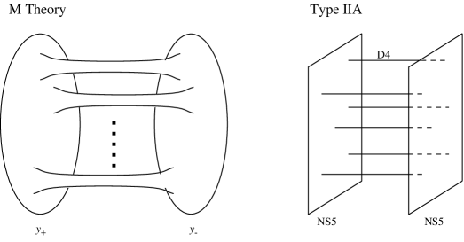
Figure 1: $M$-theory fivebrane and configuration in Type IIA theory.

2.3 $N=2$ MQCD with matter

In Type IIA picture an inclusion of $N_{f}$ matter hypermultiplets into the above pure gauge theory can be achieved by considering $N_{f}$ D sixbranes with worldvolume $(x^{0},x^{1},x^{2},x^{3},x^{7},x^{8},x^{9})$ and then putting these sixbranes between two NS fivebranes. In such a configuration there appears $N=2$ $SU(N_{c})$ supersymmetric QCD with $N_{f}$ flavors on their common worldvolume $(x^{0},x^{1},x^{2},x^{3})$. This is because the open string sector between $N_{c}$ D fourbranes and $N_{f}$ D sixbranes of the configuration gives hypermultiplets which belong to the fundamental representations both of the gauge and flavor groups.

D sixbranes could be regarded as the “Kaluza-Klein monopoles” of $M$-theory compactified to Type IIA theory with a circle $S^{1}$, since they are magnetically charged with respect to the $U(1)$ gauge field associated with $S^{1}$. The $N_{f}$ sixbranes transmute [20] the flat space $Q_{0}={\bf R}^{3}\times S^{1}$ into the multi Taub-NUT space $Q$, which is still hyper-Kähler manifold. Since the sixbranes play the role of matter hypermultiplets, the Seiberg-Witten curve which is a part of the fivebrane in $M$-theory changes to the curve of $N=2$ supersymmetric QCD with $N_{f}$ flavors [19, 30]

$$y^{2}-2\prod_{a=1}^{N_{c}}(v-\phi_{a})y+\Lambda^{2N_{c}-N_{f}}\prod_{i=1}^{N_{f}}(v-e_{i})=0,$$ (2.7)

where $e_{i}$ are the bare masses of the matter hypermultiplets and identified with the positions of the sixbranes in $v$-plane. Now the above curve is embedded in the multi Taub-NUT space $Q$.

To provide a detailed description of the embedding of curve (2.7) into the multi Taub-NUT space $Q$, we will first deal with the multi Taub-NUT metric. The multi Taub-NUT metric has the following standard form [21]

$$ds^{2}=\frac{V}{4}d{\vec{r}}^{2}+\frac{1}{4V}(d\sigma+\vec{\omega}\cdot d\vec{r})^{2},$$ (2.8)

where we introduce the coordinates $\vec{r}$ and $\sigma$ of the four-dimensional space $Q$. The potential $V$ is given by

$$V=1+\sum_{i=1}^{N_{f}}\frac{1}{|\vec{r}-\vec{r}_{i}|},$$ (2.9)

where $\vec{r}_{i}$ represents the position of the $i$-th sixbrane. The $U(1)$ gauge field $A=\vec{\omega}\cdot d\vec{r}$ is determined by the relation

$$\vec{\nabla}\times\vec{\omega}=\vec{\nabla}V.$$ (2.10)

Since $Q$ is a hyper-Kähler manifold it will have a complex structure which fits curve (2.7). With such a complex structure one may expect that the multi Taub-NUT metric becomes Kähler. In order to describe it, let us separate $\vec{r}$ into two parts, $b\in{\bf R}$ and $v\in{\bf C}$. Using these variables, metric (2.8) acquires the form [27]

$$ds^{2}=\frac{V}{4}dvd\bar{v}+\frac{1}{4V}\left(\frac{2dy}{y}-\delta dv\right)\overline{\left(\frac{2dy}{y}-\delta dv\right)}$$ (2.11)

with

$$V = 1+\sum_{i=1}^{N_{f}}\frac{1}{\Delta_{i}},$$ (2.12)

$$y = Ce^{-(b+i\sigma)/2}\prod_{i=1}^{N_{f}}(-b+b_{i}+\Delta_{i})^{1/2},$$ (2.13)

$$\delta = \sum_{i=1}^{N_{f}}\frac{1}{\Delta_{i}}\frac{b-b_{i}+\Delta_{i}}{v-e_{i}},$$ (2.14)

$$\Delta_{i} = \sqrt{(b-b_{i})^{2}+|v-e_{i}|^{2}},$$ (2.15)

where $C$ is a constant and $(b_{i},e_{i})$ represents again the position of the $i$-th sixbrane in this coordinate. While $y$ in eq.(2.13) is determined rather explicitly by $v,b$ and $\sigma$, one can also regard that $v$ and $y$ give the holomorphic coordinates of $Q$. With this complex structure the multi Taub-NUT metric becomes Kähler as is clear from (2.11). The Kähler form $\omega$ is given by

$$\omega=i\frac{V}{4}dv\wedge d\bar{v}+\frac{i}{4V}\left(\frac{2dy}{y}-\delta dv\right)\wedge\overline{\left(\frac{2dy}{y}-\delta dv\right)},$$ (2.16)

and the holomorphic two-form $\Omega$ becomes

$$\Omega=\frac{i}{2}dv\wedge\frac{dy}{y},$$ (2.17)

which satisfies the relation, $\frac{1}{2}\omega\wedge\omega=\Omega\wedge\bar{\Omega}$.

Instead of $y$ in (2.13) one can also take another choice of the holomorphic coordinates of $Q$ which corresponds to another branch of curve (2.7). It can be given by the holomorphic coordinates $(v,z)$, where $z$ is introduced by

$$z=C^{\prime}e^{(b+i\sigma)/2}\prod_{i=1}^{N_{f}}\frac{v-e_{i}}{|v-e_{i}|}(b-b_{i}+\Delta_{i})^{1/2}.$$ (2.18)

Notice that $z$ is related to $y$ by the relation

$$yz=\Lambda^{2N_{c}-N_{f}}\prod_{i=1}^{N_{f}}(v-e_{i}).$$ (2.19)

Eq. (2.19) shows that $Q$ describes a resolution of $A_{N_{f}-1}$ simple singularity, $yz=v^{N_{f}}$. It is resolved by a chain of $(N_{f}-1)$ holomorphic two-cycles. Each two-cycle intersects the next at the position of one of these $N_{f}$ sixbranes. Let us denote a two-cycle between two sixbranes $(e_{i},b_{i})$ and $(e_{i+1},b_{i+1})$ by $C_{i}$. Integrals of the two-forms $\omega$ and $\Omega$ on $C_{i}$ become [27]

$$\int_{C_{i}}\Omega = \pi(e_{i+1}-e_{i}),$$ (2.20)

$$\int_{C_{i}}\omega = 2\pi(b_{i+1}-b_{i}),$$ (2.21)

which give the difference between the positions of these two sixbranes.

The curve $\Sigma$ described by eq.(2.7) is embedded into $Q$ by using the holomorphic coordinates $(v,y)$ given above. Since $y$ is related with $b$ and $\sigma$ by eq.(2.13) it makes possible to describe the embedding of the curve $\Sigma$, say, in $(v,b)$-space. Some cases are sketched in Fig.2.

Figure 2: Sections of the Seiberg-Witten curves $\Sigma$ in $M$ theory. (a) is for asymptotically free theory ($N_{f}<2N_{c}$), (b) is for IR free theory ($N_{f}>2N_{c}$) and (c) is for finite theory ($N_{f}=2N_{c}$). The distance of two NS fivebranes at large $v$ is infinite, zero and finite, respectively.

2.4 Membranes and BPS states

In this subsection we classify the BPS states of $N=2$ MQCD according to the topology of membrane.

Let us consider a membrane which worldvolume is ${\bf R}\times D$, where a two-dimensional surface $D$ is embedded into $Q$ with its boundary $C=\partial D$ lying on the curve $\Sigma$. Area of the membrane, which is proportional to the membrane mass, satisfies the inequality [23, 24, 25, 26]

$$A_{D}\geq\frac{1}{2}\left|\int_{D}\Omega_{D}\right|,$$ (2.22)

where $\Omega_{D}$ is the pull-back to $D$ of the holomorphic two-form (2.17). $\Omega_{D}$ can be written as an exact form on $D$, that is, $\Omega_{D}=d\lambda$ where $\lambda=\frac{i}{2}v\frac{dy}{y}$. Then the integral in the r.h.s. of inequality (2.22) can be evaluated as a boundary integral

$$\int_{D}\Omega_{D}=\oint_{C}\lambda.$$ (2.23)

This boundary integral is nothing but the Seiberg-Witten mass formula for four-dimensional $N=2$ theories. In particular $\lambda$ can be regarded as the Seiberg-Witten differential [2, 3]. Thus the membrane of minimal area gives the BPS saturated state of $N=2$ MQCD with its mass being its area up to the membrane tension.

Quantum numbers of the BPS saturated state or the membrane of minimal area can be read from homology class $[C]$ of its boundary in $H_{1}(\Sigma,{\bf Z})$. We will examine some simple examples of these BPS saturated membranes.

Gauge fields and W bosons appear as Type IIA strings stretching between same or different D fourbranes. In $M$-theory, since IIA string corresponds to a membrane wrapping around a circle of the compactified eleven-dimension, gauge fields and W bosons can be identified cylindrical membranes connecting between cycles $\alpha_{i}$ on the curve $\Sigma$. $\alpha_{i}$ is a closed path surrounding the $i$-th branch cut on the Riemann sheet of $\Sigma$. If two cycles are coincident the corresponding membrane of minimal area represents gauge boson, otherwise W boson. Both states are electrically charged and integrals (2.23) on the cycles $\alpha_{i}$ give their correct BPS masses.

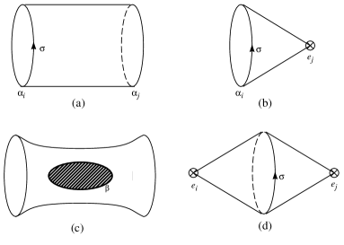
Figure 3: Topology of the minimal surfaces in $Q$ corresponding to the BPS saturated states in $N=2$ MQCD. (a) electrically charged gauge boson or W boson in vector multiplet. (b) electrically charged quark with bare mass $e_{j}$ in hypermultiplet. (c) magnetically charged monopole in hypermultiplet. (d) gauge singlet quark - anti-quark bound state. (“meson”.)

Electrically charged matter (quark) hypermultiplets are Type IIA strings between D fourbranes and D sixbranes. In $M$-theory they are the membranes connecting the cycles $\alpha_{i}$ and the sixbranes. Topology of these membranes is a disk with a puncture at the position of the sixbrane. It is like a cone. Since the Seiberg-Witten differential $\lambda$ has a pole at $v=e_{j}$ with its residue equal to the bare mass $e_{j}$, the BPS mass of the membrane is sum of the period along the cycle $\alpha_{i}$ and the bare mass $e_{j}$. This also agree with the result of [3].

Monopole is a magnetically charged hypermultiplet. Therefore the boundary of the corresponding membrane must be on a cycle $\beta_{i}$ dual to $\alpha_{i}$. Topology of this membrane is a disk. Therefore integral (2.23) gives the correct monopole mass.

Finally, let us consider a slight curious state in $N=2$ MQCD. Suppose that two membranes representing quark hypermultiplets have their common boundary on the $\alpha$-cycles of $\Sigma$. If one paste these two membranes along their common boundary, one can obtain another membrane which have a sphere topology with two punctures at the positions of the sixbranes. This state is not charged under the gauge group. This gauge singlet state will represent the quark and anti-quark bound state, that is, “meson” hypermultiplet $M^{i}_{j}=Q^{i}_{a}\tilde{Q}^{a}_{j}$. However, since this membrane does not end on the fivebrane, the state does not appear in the worldvolume effective theory on ${\bf R}^{1,3}$. So we must add the worldvolume ${\bf R}^{1,3}$ to the “meson” and regard it as a fivebrane with worldvolume ${\bf R}^{1,3}\times S^{2}$, where $S^{2}$ is a two-sphere in the multi Taub-NUT space $Q$.

This two-sphere in $Q$ can be identified with the two-cycle which resolve the simple singularity. When the theory enter the Higgs branch, a part of the fivebrane described by the curve begins to wrap the two-cycle and divides into “meson” parts [1]. According to the analysis of the embedding of the curve into $Q$, the number of these fivebranes wrapping the two-cycles is exactly equal to the dimensions of the Higgs branch [14, 27]. Therefore the above “meson” variables parameterize the moduli space of the Higgs branch.

3 Baryonic branch root of MQCD

In this section we will examine the root of baryonic branch from the MQCD view-point. The baryonic branch and the Coulomb branch encounter with each other at this root. Field theoretical analysis [10] shows that the baryonic branch root is a single point where the underlying theory is invariant under the ${\bf Z}_{2N_{c}-N_{f}}$ discrete symmetry (anomaly-free subgroup of the classical $U(1)_{R}$ symmetry). Though the $SU(N_{c})$ gauge symmetry is broken to $U(1)^{N_{c}-1}$ at a generic point of the Coulomb branch, $SU(N_{f}-N_{c})\times U(1)^{2N_{c}-N_{f}}$ non-Abelian gauge symmetry is allowed at this root and the corresponding gauge theory can be regarded as a IR-effective theory of the root. Moreover, this IR-free $SU(N_{f}-N_{c})\times U(1)^{2N_{c}-N_{f}}$ gauge theory has $2N_{c}-N_{f}$ massless singlet hypermultiplets charged only by the $U(1)$ factors in addition to $N_{f}$ quark hypermultiplets which belong to the fundamental representations of $SU(N_{f}-N_{c})$. A baryonic branch of this IR-effective theory exactly coincides with the baryonic branch of the original microscopic $SU(N_{c})$ theory. Original microscopic theory and IR-effective theory will be called respectively as “electric” theory and “magnetic” theory.

If one flows the IR-effective theory of the baryonic branch root from $N=2$ to $N=1$ by giving a mass to the adjoint scalar field, we naively expect to obtain $N=1$ $SU(N_{f}-N_{c})$ gauge theory, which is a non-Abelian dual to the original gauge theory. In terms of brane configuration this flow can be interpreted as a rotation of a part of fivebrane [13, 14, 15]. While this observation, the non-Abelian duality of $N=1$ gauge theories can be explained as the exchange of a NS fivebrane and rotated one in the $N=1$ brane configuration of Type IIA theory [7] and $M$-theory[12].

If these two operations are reversible, we may first exchange fivebranes in $M$-theory configuration and expect the same result after the rotation. Since the brane exchange could be related with the strong coupling dynamics of string theory, to consider it first in the Taub-NUT geometry, which is rather tractable than the Calabi-Yau threefold, will provide new insight on the duality. In order to exchange fivebranes in the $M$-theory configuration, we need their exact positions in the multi Taub-NUT space. As we can see in Fig.2, for the AF theory and IR-free theory the corresponding fivebrane has no definite position, but for the finite theory the position of fivebrane asymptotically approaches to a definite value since the coupling constant of the theory does not run. So we may utilize a curve of the finite theory in our description of the brane exchange in $M$-theory.

3.1 Configuration of fivebrane inspired by finite theory curve

Let us first recall that the Seiberg-Witten curve of $N_{f}=2N_{c}$ finite theory has the form [30, 10]

$$y^{2}-2\prod_{a=1}^{N_{c}}(v-\phi_{a})y-h(h+2)\prod_{j=1}^{2N_{c}}(v-he_{S}-e_{j})=0,$$ (3.1)

where $e_{S}=\frac{1}{2N_{c}}\sum e_{j}$ is the center of the bare masses $e_{j}$. $h$ is a specific modular function of the bare coupling constant $\tau=\frac{\theta}{\pi}+\frac{8\pi i}{g^{2}}$ and is given by

$$h(\tau)=\frac{2\lambda(\tau)}{1-2\lambda(\tau)}.$$ (3.2)

Notice that $\lambda(\tau)$ is the following automorphic function

$$\lambda(\tau)=16q\prod_{n=1}^{\infty}\left(\frac{1+q^{2n}}{1+q^{2n-1}}\right)^{8}$$ (3.3)

with $q=e^{\pi i\tau}$. The modular transformation of $\lambda(\tau)$ are [31]

$$T : \lambda(\tau+1)=\frac{\lambda(\tau)}{\lambda(\tau)-1},$$ (3.4)

$$S : \lambda(-1/\tau)=1-\lambda(\tau),$$ (3.5)

which implies that $\lambda(\tau)$ is invariant under the action of the congruence subgroup of level 2

$$\Gamma(2)=\left\{\left(\left.\begin{array}[]{cc}a&b\\ c&d\end{array}\right)\in SL(2,{\bf Z})~{}\right|~{}b,c~{}~{}\mbox{even}\right\}.$$ (3.6)

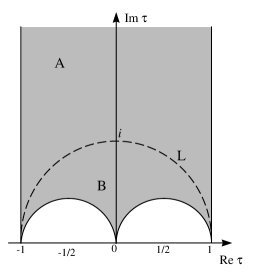
Figure 4: Fundamental domain ${\cal F}$ for $\Gamma(2)$.

Let ${\cal F}$ be a fundamental domain for $\Gamma(2)$ depicted in Fig.4. The function $\lambda(\tau)$ maps the set ${\cal F}$, one-to-one, onto ${\bf C}\cup\{\infty\}$. Since $\lambda(\tau)$ satisfies the relation $\overline{\lambda(\tau)}=\lambda(-\bar{\tau})$, it follows that ${\rm Re}~{}\lambda(\tau)=1/2$ for ${}^{\forall}\tau\in L\equiv{\cal F}\cap\{~{}\tau~{}|~{}|\tau|=1\}$. Moreover, one can find that

$$\left\{\begin{array}[]{ccc}{\rm Re}~{}\lambda(\tau)<1/2&{\rm in}&A\equiv{\cal F}\cap\{~{}\tau~{}|~{}|\tau|>1\},\\ {\rm Re}~{}\lambda(\tau)>1/2&{\rm in}&B\equiv{\cal F}\cap\{~{}\tau~{}|~{}|\tau|<1\}.\end{array}\right.$$ (3.7)

These properties of $\lambda(\tau)$ will be important for later discussions.

As a result, $h(\tau)$ satisfies the modular property $h\rightarrow-(h+2)$ under $\tau\rightarrow-1/\tau$. Therefore, the Seiberg-Witten curve (3.1), which describes the Coulomb branch of the theory, is invariant under $S$-transformation if the bare masses admit to be transformed as

$$\left\{\begin{array}[]{lcl}e_{j}&\rightarrow&e_{j}-2e_{S},\\ e_{S}&\rightarrow&-e_{S}.\end{array}\right.$$ (3.8)

With these transformations the Coulomb branch acquires a $SL(2,{\bf Z})$ symmetry. We may call it the $SL(2,{\bf Z})_{V}$ symmetry since the Coulomb branch is the moduli space of vector multiplets.

Now let us examine a family of the baryonic branch root embedded in the finite theory. Since the baryonic branch has the ${\bf Z}_{2N_{c}-N_{f}}$ symmetry, we require first the finite theory curve to have this symmetry. By this requirement the vevs of the adjoint scalar field and the bare masses must be of the form

$$\phi_{a} = (0,\ldots,0,\varphi\omega,\varphi\omega^{2},\ldots,\varphi\omega^{2N_{c}-N_{f}}),$$ (3.9)

$$e_{j} = (\underbrace{0,\ldots,0}_{N_{f}-N_{c}},m\omega,m\omega^{2},\ldots,m\omega^{2N_{c}-N_{f}}),$$ (3.10)

where $\omega^{2N_{c}-N_{f}}=1$. Then, curve (3.1) becomes

$$y^{2}-2v^{N_{f}-N_{c}}(v^{2N_{c}-N_{f}}-\varphi^{2N_{c}-N_{f}})y-h(h+2)v^{N_{f}}(v^{2N_{c}-N_{f}}-m^{2N_{c}-N_{f}})=0.$$ (3.11)

Further requirement on the curve is that it should be maximally degenerated at the baryonic branch root. Namely, all cycles on the curve must vanish. To establish this, we first rewrite curve (3.11) in a quadratic form of $Y=y-\prod_{a=1}^{N_{c}}(v-\phi_{a})$

$$Y^{2}=v^{2(N_{f}-N_{c})}\left\{(v^{2N_{c}-N_{f}}-\varphi^{2N_{c}-N_{f}})^{2}+h(h+2)v^{2N_{c}-N_{f}}(v^{2N_{c}-N_{f}}-m^{2N_{c}-N_{f}})\right\}.$$ (3.12)

When the r.h.s. of (3.12) becomes a perfect square, all the branches disappear and therefore all the cycles vanish. The Riemann sheets of the hyperelliptic curve are decoupled to two complex planes. This situation can occur if and only if the relation

$$m^{2N_{c}-N_{f}}=\frac{2}{-h(\tau)}\varphi^{2N_{c}-N_{f}},$$ (3.13)

or

$$m^{2N_{c}-N_{f}}=\frac{2}{h(\tau)+2}\varphi^{2N_{c}-N_{f}}$$ (3.14)

is satisfied. Note that these two relations are equivalent in the sense that modular transformation $\tau\rightarrow-1/\tau$ exchanges (3.13) and (3.14). So it is enough to study only the former without loss of generality. However, this $S$-transformation of the position of sixbranes does not satisfy (3.8). So it breaks the $SL(2,{\bf Z})_{V}$ symmetry, which means that configuration (3.13) does not belong to the category of finite theory curve, but it is still meaningful as a $M$-theory brane configuration and, after taking a suitable scaling limit, it turns out to describe the baryonic branch root.

When relation (3.13) is satisfied the curve becomes the perfect square

$$Y^{2}=v^{2(N_{f}-N_{c})}\left\{(h+1)v^{2N_{c}-N_{f}}+\varphi^{2N_{c}-N_{f}}\right\}^{2}.$$ (3.15)

Or equivalently two roots of (3.11) with respect to $y$ describe two independent complex planes without any branch

$$\left\{\begin{array}[]{rcl}y_{+}&=&(h+2)v^{N_{c}},\\ y_{-}&=&-v^{N_{f}-N_{c}}\left\{hv^{2N_{c}-N_{f}}+2\varphi^{2N_{c}-N_{f}}\right\}.\end{array}\right.$$ (3.16)

It means that the single fivebrane embedded in the multi Taub-NUT space now decouples to two parts. As we discuss subsequently these two fivebranes admit to have an intersection in the Taub-NUT space. Though the intersection itself has its origin in the branch cuts of the Riemann sheets, its behavior for a given $\tau$, if one consider it in the Taub-NUT space, is quite different depending on the value of $\tau$.

3.2 Intersection of fivebranes in the Taub-NUT space

We examine their intersection in the Taub-NUT space in detail. Recall the embeddings of two fivebranes (3.16) are given by the equations

$$\left\{\begin{array}[]{rcl}y_{+}&=&Ce^{-(b_{+}+i\sigma_{+})/2}\prod^{2N_{c}}_{j=1}(-b_{+}+b_{i}+\Delta_{i}),\\ y_{-}&=&Ce^{-(b_{-}+i\sigma_{-})/2}\prod^{2N_{c}}_{j=1}(-b_{-}+b_{i}+\Delta_{i}).\end{array}\right.$$ (3.17)

Their intersection in the Taub-NUT space can be handled by the equation $b_{+}(v)=b_{-}(v)$, which implies

$$\left|\frac{y_{+}}{y_{-}}\right|=1.$$ (3.18)

This can be regarded as an equation for $v$. The allowed values of $v$, that is, solutions of the equation, describe the intersection projected to $v$-plane. Inserting explicit forms (3.16) to (3.18), after a little calculation, we obtain

$$\left|1-\frac{M}{V}\right|=\left|1-\frac{1}{\lambda(\tau)}\right|,$$ (3.19)

where $V=v^{2N_{c}-N_{f}}$ and $M=m^{2N_{c}-N_{f}}$. An implication of eq.(3.19) may be tractable if one considers it in $V$-plane rather than $v$-plane. Now $M$ gives the sixbrane position on $V$-plane. Let us take $M$ as a positive real quantity and set $V=X+iY$. Then eq.(3.19) becomes

$$\left(X-\frac{|\lambda|^{2}M}{2\gamma-1}\right)^{2}+Y^{2}=\left|\frac{\lambda(\lambda-1)M}{2\gamma-1}\right|^{2},$$ (3.20)

where $\gamma={\rm Re}~{}\lambda$. If $\gamma\neq 1/2$ it describes a circle centered at $X_{0}\equiv\frac{|\lambda|^{2}}{2\gamma-1}M$ on $X$-axis with radius $R\equiv\left|\frac{\lambda(\lambda-1)}{2\gamma-1}\right|M$. Let us comment some details on this intersection (3.20). It can be classified into the following three cases.

When $\gamma$ is less than $1/2$ (i.e. $|\tau|>1$), it holds that $X_{0}<0$ and $0<X_{0}+R<M$. So the origin is inside of the circle and the sixbrane is located outside of the circle. When $\gamma$ is equal to $1/2$ (i.e. $|\tau|=1$), (3.19) describes a straight line between the origin and the sixbrane; $X=\frac{1}{2}M$. Finally, when $\gamma$ is greater than $1/2$ (i.e. $|\tau|<1$), it holds that $X_{0}>0$ and $0<X_{0}-R<M<X_{0}+R$. So the origin is outside of the circle while the sixbrane is inside of the circle. They are depicted in Fig.5.

Figure 5: Intersections of two fivebrane on $V$-plane.

Since $v$ is a ($2N_{c}-N_{f}$)-th root of $V$, these circles and line are copied $2N_{c}-N_{f}$ times on the original $v$-plane. Namely, the circle or line in each case becomes a single wavy circle which surrounds the origin, $2N_{c}-N_{f}$ parabolic lines or $2N_{c}-N_{f}$ circles surrounding each sixbrane, respectively. These intersections of two fivebranes in the Taub-NUT space are depicted in Fig.6.

Figure 6: Intersections of two fivebrane on $v$-plane. Dots represent the positions of the sixbranes. The case of $2N_{c}-N_{f}=6$ is sketched as an example.

3.3 Weak coupling limits

Since the intersection of fivebranes in the Taub-NUT space is realized in very different fashions depending on the value of $\tau$, it will bring us different descriptions of the ${\bf Z}_{2N_{c}-N_{f}}$ symmetric and maximally degenerate theory. There appear two regions of the fundamental domain ${\cal F}$ where the intersection is qualitatively different from each other. These two regions are separated by the semi-circle $L$. So, we can expect, at least, two completely different descriptions of the theory.

To determine the massless spectrum of each description, we will take the weak coupling limit in terms of the bare coupling constant $\tau$ or its dual $\tilde{\tau}=-1/\tau$. We first consider the case of the original “electric” theory. Let $m$ in (3.13) be a function of $\tau$ with a fixed constant $\varphi=\Lambda$. In the weak coupling limit ($\tau\rightarrow i\infty$) of the configurations, $2N_{c}-N_{f}$ sixbranes are naturally decoupled and curve (3.11) becomes

$$y^{2}-2v^{N_{f}-N_{c}}(v^{2N_{c}-N_{f}}-\Lambda^{2N_{c}-N_{f}})y-4\Lambda^{2N_{c}-N_{f}}v^{N_{f}}=0.$$ (3.21)

Note that $\lim_{\tau\rightarrow i\infty}h(\tau)=0$. This degenerated curve describes the baryonic branch root of the AF theory with color $SU(N_{c})$ and $N_{f}$ flavor. It exactly agrees with [10]. This is nothing but the desired original “electric” theory! At this baryonic branch root of the “electric” theory, the gauge symmetry is broken to $SU(N_{f}-N_{c})\times U(1)^{2N_{c}-N_{f}}$. Due to the degeneration of the curve there appear $2N_{c}-N_{f}$ mutually local massless hypermultiplets. Each of them is charged under only one $U(1)$ factor. Thus all massless fields appear as the magnetically charged solitonic states.

Next we examine the weak coupling limit of the dual bare coupling constant $\tilde{\tau}=-1/\tau$. This limit $\tilde{\tau}\rightarrow i\infty$ corresponds to the limit $\tau\rightarrow 0$ of the original bare coupling constant. So we must examine the region $|\tau|<1$. The intersection of two fivebranes is circles which surround the extra $2N_{c}-N_{f}$ sixbranes. The radius of these circles vanish in this limit. Let us pay attention to these small circles. In the Taub-NUT space they give rise to two-spheres surrounding the sixbranes and confined by the two fivebranes. These two-spheres consist of the circles and the disks in the fivebranes inside their intersection. Mathematically speaking, what we obtain here is not a two-sphere but a punctured two-sphere. This is because the sixbranes are the NUT singularities in the Taub-NUT space and there exist Dirac strings running from the sixbranes. Two-spheres obtained above must have intersections with these Dirac strings since they are surrounding the sixbranes.

On the other hand, if we look at only one side of the fivebranes, the radius of circles is also considered roughly as thickness of the fivebrane which stretches from major part lying at asymptotic position toward the sixbrane. So, in the limit $\tau\rightarrow 0$ the stretching part of the fivebrane becomes very fine. Moreover, due to aforementioned puncture on the fivebrane, this stretching part can be thought to wrap the eleventh-dimension. Then this part becomes D fourbrane stretching from NS fivebrane and touching the D sixbrane in Type IIA theory. (See Fig.7.)

This observation can be also confirmed from the curve. In the limit $\tau\rightarrow 0$, it holds $\lim_{\tau\rightarrow 0}m^{2N_{c}-N_{f}}(\tau)=\Lambda^{2N_{c}-N_{f}}$. So curve (3.11) becomes

$$y^{2}-2v^{N_{f}-N_{c}}(v^{2N_{c}-N_{f}}-\Lambda^{2N_{c}-N_{f}})y-h(h+2)v^{N_{f}}(v^{2N_{c}-N_{f}}-\Lambda^{2N_{c}-N_{f}})=0.$$ (3.22)

This describes the finite theory whose $2N_{c}-N_{f}$ D sixbranes and D fourbranes are at the same position on $v$-plane and touching each other.

The massless spectrum which we can read from the above limit of the configurations are as follows: $2N_{c}-N_{f}$ massless singlet hypermultiplets obtained from the open string connecting the extra $2N_{c}-N_{f}$ D sixbranes and the D fourbranes touching them. These hypermultiplets appear now as the elementary states. So the configuration itself describes the dual “magnetic” theory.

In both limits, $\tau\rightarrow i\infty$ and $\tau\rightarrow 0$, same massless spectrum appears, but in different fashions. Namely they appear as massless solitonic states due to the monopole singularity or massless elementary states due to the quark singularity.

Figure 7: Sections of the intersecting two fivebranes. Dots represent the sixbranes. A limit to the left ($\tau\rightarrow i\infty$) describes the baryonic branch root of $SU(N_{c})$ theory and a limit to the right ($\tau\rightarrow 0$) describes the baryonic branch root of $SU(N_{f}-N_{c})$ theory.

3.4 Brane exchange

We have seen the massless spectrum of the configuration at the boundaries of their moduli space, that is, $\tau=i\infty$ and $\tau=0$. Now consider a path in the moduli space which connects these two boundaries. In the region $|\tau|>1$ the asymptotic positions of two fivebranes for large $|v|$ can be read from (3.16)

$$\left\{\begin{array}[]{rcl}b_{+}^{as}&=&\ln|h(\tau)+2|,\\ b_{-}^{as}&=&\ln|-h(\tau)|.\end{array}\right.$$ (3.23)

These asymptotic positions coincide with each other on the semi-circle $L$, since the relative distance of the asymptotic positions satisfies

$$\Delta b^{as}=\ln\left|\frac{h(\tau)+2}{-h(\tau)}\right|=\ln\left|\frac{\lambda(\tau)-1}{\lambda(\tau)}\right|=0,$$ (3.24)

if $|\tau|=1$. And obviously two positions are exchanged under the $S$-dual transformation $\tau\rightarrow-1/\tau$. Therefore one can say that, if $\tau$ moves continuously from one region to another across the semi-circle $L$, the asymptotic positions of two fivebranes are passed each other on $L$ and exchanged.

As we have seen, this brane exchange also exchanges the solitonic states with the elementary states. Moreover, the degeneracy of the curve at the origin of $v$-plane, which only relates to the moduli space of the baryonic branch, is not affected by this exchange of branes. Therefore the baryonic branches realized in each region are exactly the same, that is, the baryonic branch of $SU(N_{c})$ MQCD with $N_{f}$ flavors is isomorphic to that of $SU(N_{f}-N_{c})$ MQCD with $N_{f}$ flavors. Thus, instead of broken $SL(2,{\bf Z})_{V}$ symmetry, there exists another $SL(2,{\bf Z})$ symmetry for the baryonic branch, that is, the moduli space of vacua for the hypermultiplets.

This situation is very similar to the explanation of Seiberg’s non-Abelian duality in $N=1$ SQCD by the exchange of Type IIA brane configurations. So if we rotate the above $N=2$ MQCD configuration and break the supersymmetry to $N=1$, it will give a proof of the $N=1$ non-Abelian duality via $M$-theory.

Appendix

Appendix A The multi Taub-NUT metric as a Kähler metric

The multi Taub-NUT space is asymptotically flat and looks near infinity like ${\bf R}^{3}\times S^{1}$. If we set the coordinates $(\vec{r},\sigma)\equiv(x^{1},x^{2},x^{3},\sigma)\in{\bf R}^{3}\times S^{1}$, where $\sigma$ is periodic $(0\leq\sigma\leq 4\pi)$, the metric is given by [21]

$$ds^{2}=\frac{V}{4}d{\vec{r}}^{2}+\frac{1}{4V}(d\sigma+\vec{\omega}\cdot d\vec{r})^{2},$$ (A.1)

where

$$V=1+\sum_{i=1}^{d}\frac{1}{|\vec{r}-\vec{r}_{i}|},$$ (A.2)

and $\vec{r}_{j}$ is a position of the $j$-th monopole in ${\bf R}^{3}$. $\vec{\omega}$ is the Dirac monopole potential, which satisfies

$$\vec{\nabla}\times\vec{\omega}=\vec{\nabla}V.$$ (A.3)

A particular solution of eq.(A.3) can be chosen as

$$\left\{\begin{array}[]{rcl}\omega_{1}&=&0,\\ \omega_{2}&=&\sum_{j=1}^{d}\frac{x^{3}-x^{3}_{j}}{|\vec{r}-\vec{r}_{j}|(x^{1}-x^{1}_{j}-|\vec{r}-\vec{r}_{j}|)},\\ \omega_{3}&=&\sum_{j=1}^{d}\frac{-x^{2}+x^{2}_{j}}{|\vec{r}-\vec{r}_{j}|(x^{1}-x^{1}_{j}-|\vec{r}-\vec{r}_{j}|)}.\end{array}\right.$$ (A.4)

Let us first substitute this solution for $\vec{\omega}\cdot d\vec{r}$ in metric (A.1),

$$\vec{\omega}\cdot d\vec{r}={\rm Im}\left(\sum_{j=1}^{d}\frac{1}{|\vec{r}-\vec{r}_{j}|}\frac{b-b_{j}+|\vec{r}-\vec{r}_{j}|}{v-e_{j}}dv\right),$$ (A.5)

where $b\equiv x^{1}\in{\bf R}$ and $v\equiv x^{2}+ix^{3}\in{\bf C}$. The position of the $j$-th monopole is rewritten in this coordinates as $\vec{r}_{j}\mapsto(b_{j},e_{j})$. We also define the following quantities for later convenience:

$$\Delta_{j} \equiv |\vec{r}-\vec{r}_{j}|$$

$$= \sqrt{(b-b_{j})^{2}+|v-e_{j}|^{2}},$$

$$\delta \equiv \sum_{j=1}^{d}\frac{1}{\Delta_{j}}\frac{(b-b_{j})+\Delta_{j}}{v-e_{j}}.$$ (A.7)

Then (A.5) simply becomes

$$\vec{\omega}\cdot d\vec{r}={\rm Im}(\delta dv).$$ (A.8)

Next we introduce the quantity

$$y\equiv Ce^{-(b+i\sigma)/2}\prod_{j=1}^{d}(-b+b_{j}+\Delta_{j})^{1/2},$$ (A.9)

where $C$ is some constant. After some straightforward calculation we can find

$$\frac{2dy}{y}=-Vdb-id\sigma+{\rm Re}(\delta dv).$$ (A.10)

Using eq.(A.10) the following equalities can be shown:

$$\left(\frac{2dy}{y}-\delta dv\right)\overline{\left(\frac{2dy}{y}-\delta dv\right)} = \left\{{\rm Re}\left(\frac{2dy}{y}-\delta dv\right)\right\}^{2}+\left\{{\rm Im}\left(\frac{2dy}{y}-\delta dv\right)\right\}^{2}$$ (A.11)

$$= V^{2}db^{2}+\{d\sigma+{\rm Im}(\delta dv)\}^{2}.$$

Finally, inserting eq.(A.8) into metric (A.1) and rewriting it using eq.(A.11), the multi Taub-NUT metric acquires the form of a Kähler metric:

$$ds^{2} = \frac{V}{4}(db^{2}+dvd\bar{v})+\frac{1}{4V}\{d\sigma+{\rm Im}(\delta dv)\}^{2}$$ (A.12)

$$= \frac{V}{4}dvd\bar{v}+\frac{1}{4V}\left(\frac{2dy}{y}-\delta dv\right)\overline{\left(\frac{2dy}{y}-\delta dv\right)}.$$ (A.13)

Appendix B Integrals on vanishing two-cycles in the multi Taub-NUT space

A vanishing two cycle $C_{j}$ between two monopoles at $(b_{j},e_{j})$ and $(b_{j+1},e_{j+1})$ can be represented in $(b,v)$-space as a line

$$\left\{\begin{array}[]{rcl}b&=&\lambda(b_{j+1}-b_{j})+b_{j},\\ v&=&\lambda(e_{j+1}-e_{j})+e_{j},\end{array}\right.$$ (B.1)

where $\lambda$ is a real parameter, $0\leq\lambda\leq 1$. Let $y(\lambda,\sigma)$ be a function defined by restricting $y$ on $C_{j}$, that is, $y(\lambda,\sigma)\equiv y|_{C_{j}}$. Using the explicit form (A.9) of $y$, $y(\lambda,\sigma)$ turns out to have the form:

$$y(\lambda,\sigma)=e^{-i\sigma/2}f(\lambda),$$ (B.2)

where a function $f(\lambda)$ is independent of $\sigma$ and satisfies $f(0)=f(1)=0$.

Integrals of the holomorphic two-form $\Omega$ on $C_{j}$ become as follows:

$$\int_{C_{j}}\Omega = \frac{i}{2}\int_{C_{j}}dv\wedge d\ln y(\lambda,\sigma)$$ (B.3)

$$= \frac{1}{4}(e_{j+1}-e_{j})\int_{0}^{1}d\lambda\int_{0}^{4\pi}d\sigma$$

$$= \pi(e_{j+1}-e_{j}),$$

while integrals of the Kähler two-form are slightly entangled:

$$\int_{C_{j}}\omega = \frac{i}{4}\int_{C_{j}}\frac{1}{V}\left(\frac{2dy}{y}-\delta dv\right)\wedge\overline{\left(\frac{2dy}{y}-\delta dv\right)}$$ (B.4)

$$= \frac{i}{4}\int_{C_{j}}\frac{1}{V}\left\{Vdb+id\sigma+i{\rm Im}(\delta dv)\right\}\wedge\left\{Vdb-id\sigma-i{\rm Im}(\delta dv)\right\}$$

$$= \frac{1}{2}\int_{C_{j}}\left\{db\wedge d\sigma+{\rm Im}(\delta dv)\wedge db\right\}$$

$$= \frac{1}{2}\int_{C_{j}}db\wedge d\sigma$$

$$= 2\pi(b_{j+1}-b_{j}),$$

where we use the fact that ${\rm Im}(\delta dv)\wedge db$ vanish on $C_{j}$.

References

- [1] E. Witten, “Solutions of Four-Dimensional Field Theories via M Theory”, Nucl. Phys. B500 (1997) 3, hep-th/9703166.
- [2] N. Seiberg and E. Witten, “Electric-Magnetic Duality, Monopole Condensation, and Confinement in N=2 Supersymmetric Yang-Mills Theory,” Nucl. Phys. B426 (1994) 19, hep-th/9407087.
- [3] N. Seiberg and E. Witten, “Monopoles, Duality and Chiral Symmetry Breaking in N=2 Supersymmetric QCD,” Nucl. Phys. B431 (1994) 484, hep-th/9408099.
- [4] N. Seiberg, “Electric - Magnetic Duality in Supersymmetric Non-Abelian Gauge Theories”, Nucl. Phys. B435 (1995) 129, hep-th/9411149.
- [5] K. Intriligator and N. Seiberg, “Lectures on Supersymmetric Gauge Theories and Electric - Magnetic Duality”, Nucl. Phys. Proc. Suppl. 45BC (1996) 1, hep-th/9509066.
- [6] A. Hanany and E. Witten, “Type IIB Superstrings, BPS Monopoles, and Three-dimensional Gauge Dynamics”, Nucl. Phys. B492 (1997) 152, hep-th/9611230.
- [7] S. Elitzur, A Giveon and D. Kutasov, “Branes and N=1 Duality in String Theory”, Phys. Lett. B400 (1997) 269, hep-th/9702014.
- [8] E. Witten, “String Theory Dynamics in Various Dimension”, Nucl. Phys. B443 (1995) 85, hep-th/9503124.
- [9] R. G. Leigh and M. J. Strassler, “Exactly Marginal Operators and duality in Four-dimensional N=1 Supersymmetric Gauge Theory”, Nucl. Phys. B447 (1995) 95, hep-th/9503121.
- [10] P. C. Argyres, M. R. Plesser and N. Seiberg, “The Moduli Space of Vacua of N=2 SUSY QCD and Duality in N=1 SUSY QCD,” Nucl. Phys. B471 (1996) 159, hep-th/9603042.
- [11] T. Hirayama, N. Maekawa and S. Sugimoto, “Deformations of N=2 Dualities to N=1 Dualities in , and Gauge Theories”, hep-th/9705069.
- [12] M. Schmaltz and R. Sundrum, “N=1 Field Theory Duality from M Theory”, hep-th/9708015.
- [13] J. L. F. Barbon, “Rotated Branes and N=1 Duality”, hep-th/9703051.
- [14] K. Hori, H. Ooguri and Y.Oz, “Strong Coupling Dynamics of Four-Dimensional N=1 Gauge Theories from M theory Fivebrane”, hep-th/9706082.
- [15] E. Witten, “Branes and The Dynamics of QCD”, hep-th/9706109.
- [16] E. Verlinde, “Global Aspects of Electric - Magnetic Duality”, Nucl. Phys. B455 (1995) 211, hep-th/9506011.
- [17] A. Klemm, W. Lerche, S. Yankielowicz, “Simple Singularities and Supersymmetric Yang-Mills Theory,” Phys. Lett. B344 (1995) 169, hep-th/9411048.
- [18] P. C. Argyres and A. E. Faraggi, “The Vacuum Structure and Spectrum of Supersymmetric Gauge Theory,” Phys. Rev. Lett. 74 (1995) 3931, hep-th/9411057.
- [19] A. Hanany and Y. Oz, “On the Quantum Moduli Space of Vacua of Supersymmetric Gauge Theories,” Nucl. Phys. B452 (1995) 283, hep-th/9505075.
- [20] P. K. Townsend, “ The eleven-dimensional supermembrane revisited”, Phys. Lett. B350 (1995) 184, hep-th/9501068.
-
[21]
S. W. Hawking, “Gravitational Instantons,” Phys. Lett. 60A (1977) 81.
G. W. Gibbons and S. W. Hawking, “Classification of Gravitational Instanton Symmetries”, Commun. Math. Phys. 66 (1979) 291.
T. Eguchi, B. Gilkey and J. Hansen, Phys. Rep. 66 (1980) 213. - [22] N. J. Hitchin, “Polygons and gravitons”, Math. Proc. Camb. Phil. Soc. 85 (1979) 465.
- [23] A. Fayyazuddin and M. Spalinski, “The Seiberg-Witten Differential from M Theory”, Nucl. Phys. B508 (1997) 219, hep-th/9706087.
- [24] M. Henningson and P. Yi, “Four-dimensional BPS-spectra via M-theory”, hep-th/9707251.
- [25] A. Mikhailov, “BPS States and Minimal Surfaces”, hep-th/9708068.
- [26] A. Fayyazuddin and M. Spalinski, “Extended Objects in MQCD”, hep-th/9711083.
- [27] T. Nakatsu, K. Ohta, T. Yokono and Y. Yoshida, “Higgs Branch of N=2 SQCD and M Theory Branes”, hep-th/9707258.
- [28] T. Nakatsu, K. Ohta, T. Yokono and Y. Yoshida, “A Proof of Brane Creation via M theory”, hep-th/9711117.
- [29] Y. Yoshida, “Geometrical Analysis of Brane Creation via -theory”, hep-th/9711177.
- [30] P. C. Argyres, M. R. Plesser and A. D. Shapere, “The Coulomb Phase of N=2 Supersymmetric QCD,” Phys. Rev. Lett. 75 (1995) 1699, hep-th/9505100.
-
[31]
L. R. Ford, “Automorphic Functions”, Chelsea Publishing, New York.
E. T. Whittaker and G. W. Watson, “A Course of Modern Analysis”, Cambridge University Press.