Dimensional reduction of the chiral-continous Gross-Neveu model

G.N.J.Añaños, A.P.C.Malbouisson, M.B.Silva-Neto and N.F.Svaiter*
Centro Brasileiro de Pesquisas Fisicas-CBPF

Rua Dr.Xavier Sigaud 150, Rio de Janeiro, RJ 22290-180 Brazil

We study the finite-temperature phase transition of the generalized Gross-Neveu model with continous chiral symmetry in $2<d\leq 4$ euclidean dimensions. The critical exponents are computed to the leading order in the $1/N$ expansion at both zero and finite temperatures. A dimensionally reduced theory is obtained after the introduction of thermal counterterms necessary to cancel thermal divergences that arise in the limit of high temperature. Although at zero temperature we have an infinitely and continously degenerate vacuum state, we show that at finite temperature this degeneracy is discrete and, depending on the values of the bare parameters, we may have either total or partial restoration of symmetry. Finally we determine the universality class of the reduced theory by a simple analysis of the infrared structure of thermodynamic quantities computed using the reduced action as starting point.

Pacs numbers: 11.10.Ef, 11.10.Gh

1 Introduction

One of the differences between field theories and mechanical systems is that field theories have an infinite number of degrees of freedom, which makes possible spontaneous symmetry breaking. More generally, we know, by now, that also dynamical symmetry breaking plays an important role in modern physics. In condensed matter physics, for example, such a mechanism is used to describe superconductivity, by the condensate of Cooper pairs, while for particle physics it is the main source of hadron masses and governs the low energy hadron dynamics.

Connected with dynamical symmetry breaking comes the problem of restoration of broken symmetries for some sufficiently high temperature. As it is well known, a phase transition occurs when there is a singularity in the free energy or one of its derivatives. The fact that almost all phenomena studied in theories near the transition point exhibit scaling, that is, a power-law behavior between two mesurable quantities, leads naturally to the classification of different conformal field theories in universality classes, which are itself determined by a set of numbers usually called critical indices.

A large number of conformal field theories is known in two dimensions and none is firmly established in four. The dimensionality $(d=3)$ is between these extremes and contains two well established families of conformal field theories. The first family contains the usual Ising, XY and Heisenberg critical $\sigma$ models and is characterized by a particular set of exponents called scalar critical exponents. The second family contains various critical four fermion models [1] and the set of exponents that characterizes it is called chiral critical exponents. The critical properties of the great majority of phase transitions in three euclidean dimensions (magnetic systems, superconductors etc.) are quite accurately described by the first family of conformal field theories while the finite-temperature phase transitions in certain $(3+1)$ dimensional quantum field theories are argued to belong to these same universality classes [2].

When studying the finite-temperature chiral restoration in QCD one is usually gided by the concepts of dimensional reduction and universality. From the dimensional reduction point of view, a hot field theory can be regarded as a static field theory at zero temperature in a lower dimension [3]. For example, four dimensional QCD with $N_{f}$ light quarks near the transition can be described by the three dimensional linear $\sigma$ model with the same global symmetry [4]. On the other hand, as the classification in universality classes is done by the computation of critical indices and those critical indices are infrared (IR) sensitive, we must understand the role of each degree of freedom in this context. This can be easily done with the use of effective field theory methods in which the integration over different energy scales gives a theory for the degrees of freedom which are the real responsible for infrared divergencies [5]. Dimensional reduction is based in the zero temperature Appelquist-Carazone decoupling theorem [6], where a low energy theory is constructed by the integration over heavy fields in the functional integral.

According to standard dimensional reduction arguments, the fermions themselves, even if they are massless at zero temperature, do not influence the nature of phase transition at finite-temperature. It is rather their bosonic composites, the Goldstone bosons, which are of importance. This follows directly from the universality of second order phase transitions [7], in which the commonly held assumption is that all the possible universality classes (or equivalently, conformal field theories) are variations of the $\sigma$ model and one need only match the correct symmetry-breaking pattern. As a consequence, the chiral transition of four dimensional QCD, with $N_{f}=2$ flavors, should lie in the same universality class as a three dimensional $O(4)$ magnet. Similarly, other models, e.g. four-fermion theories in $d$ dimensions such as the Gross-Neveu model (GN model) [8] with discrete symmetries or the Nambu-Jona-Lasinio model (NJL model) [9] with continous chiral symmetry, are expected to be in the same universality class of a $(d-1)$ dimensional Ising or Heisenberg magnet, respectively.

Recently, however, it was pointed out that there exist different $(d=3)$ conformal field theories with the same symmetry-breaking pattern [1]. They are exactly the four-fermion interaction models of the Nambu-Jona-Lasinio type. Physically, this corresponds to the fact that on the chirally symmetric side of the phase transition there are $N$ massless fermions whose effect is felt even in the IR fixed point, just like the Goldstone bosons. The presence of more than one universality class in $(d=3)$ makes the procedure of dimensionally reducing a quantum field theory ambigous and it is now uncertain to which conformal field theory the $(d+1)$ finite-temperature quantum field theory will reduce. The argument if favor of the bosonic universality class goes as follows. At finite-temperature, the $(d=4)$ fermion reduces to a collection of $(d=3)$ massive fermions and there is no zero mode for which the Matsubara frequency vanishes. Nevertheless, even if a single massive field does not influence the phase transition, the cumulative effects of an infinite number of such fields may have an appreciable impact. In order to see whether or not this happens, all harmonics should be summed and their cumulative effects studied.

It is the purpose of this paper to discuss the assumptions underlying this analysis and to determine to which universality class the simplest generalization of the Gross-Neveu model with continous chiral symmetry, belongs. Besides being an interesting theoretical model, it is also believed that, when properly extended to incorporate continous chiral symmetry, four-fermion models are more realistic as effective theories of QCD than the linear $\sigma$ model, especially at scales where quark structure is important.

The paper is organized as follows. In section II, we present the model. In section III we compute the critical exponents at zero temperature while, in section IV, we obtain, after dimensional reduction, the new critical exponents that determines the universality class of the reduced theory. In section V, we analyse the vacuum structure at finite-temperature. Conclusions are given in section VII. In the appendix, we compute the thermal renormalization group functions that controlls thedependence of the thermal counterterms on the temperature. In this paper we use $h\!\!\!/=c=1$.

2 The chiral-continous GN model

We are interested in studying the behavior of a multiplet of N fermions coupled with a pair of composite self-interacting pseudo-scalar and scalar fields, $\sigma(x)$ and $\pi(x)$ respectively, in such a way that the euclidean functional action reads

$$S_{E}=\int d^{d}{\bf x}\left\{-\bar{\psi}\left(\partial\!\!\!/+g_{B}\left(\sigma+i\gamma_{S}\pi\right)\right)\psi+\frac{1}{2}(\partial_{\mu}\sigma)^{2}+\frac{1}{2}(\partial_{\mu}\pi)^{2}-\frac{1}{2}m_{B}^{2}\left({\sigma}^{2}+{\pi}^{2}\right)+\frac{\lambda_{B}}{4}\left({\sigma}^{2}+{\pi}^{2}\right)^{2}\right\}.$$ (1)

This model has continous chiral symmetry

$$\left\{\begin{array}[]{ll}\bar{\psi}\rightarrow\bar{\psi}e^{i\alpha\gamma_{s}}\\ \psi\rightarrow e^{i\alpha\gamma_{s}}\psi,\end{array}\right.,$$ (2)

and $\sigma\rightarrow-\sigma$, $\pi\rightarrow\pi$ with $\alpha$ being a constant and we use for the $\gamma_{s}$ the following representation $\gamma_{S}=\left(\begin{array}[]{ll}1&0\\ 0&-1\end{array}\right)$.

In order to have an uniquely defined vacuum (see fig. 1), we must choose a prefered direction in the space of components, say $\left<\sigma\right>=v$ and $\left<\pi\right>=0$, and shift our fields as

$$\left\{\begin{array}[]{ll}\sigma(x)\rightarrow v+\sigma(x)\\ \pi(x)\rightarrow\pi(x)\end{array}\right.,$$ (3)

where $v=\frac{\sqrt{m_{B}}}{\lambda_{B}}$. In this new picture the euclidean action becomes

$$S_{E} = \int d^{d}{\bf x}\left\{-\frac{1}{2}m_{B}^{2}v^{2}+\frac{\lambda_{B}}{4}v^{4}-\bar{\psi}\left(\partial\!\!\!/+g_{B}\left(v+\sigma+i\gamma_{S}\pi\right)\right)\psi+\frac{1}{2}(\partial_{\mu}\sigma)^{2}+\frac{1}{2}(\partial_{\mu}\pi)^{2}\right.$$ (4)

$$- \left.\frac{1}{2}m_{\sigma}^{2}\sigma^{2}-\frac{1}{2}m_{\pi}^{2}\pi^{2}-{\lambda_{B}}v{\sigma^{3}}-{\lambda_{B}}v{\sigma}{\pi^{2}}+\frac{\lambda_{B}}{4}\left({\sigma}^{2}+{\pi}^{2}\right)^{2}\right\},$$ (5)

with $m_{\sigma}=m_{B}^{2}-3\lambda_{B}v^{2}$ and $m_{\pi}=m_{B}^{2}-\lambda_{B}v^{2}$. If we use the definition of $v$ we can see that $m_{\pi}=0$, as it should be since the $\pi$ field is a Goldstone boson. Although new interaction terms have arised, it is easy to prove that this renormalizable model needs only usual wave function, mass and coupling constant renormalization to render the theory finite.

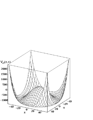
Figure 1: Mexican hat shape for the zero temperature effective potential in the tree level. The vacuum is infinitely degenerate and one of the degrees of freedom will become a Goldstone boson after the definition of an unique ground-state.

The finite-temperature version of this model is obtained, in the Matsubara formalism, by the compactification of the imaginary time dimension together with the imposition of (anti)-periodic boundary conditions to (fermionic)-bosonic fields [3] as

$$\bar{\psi}({\bf x},\tau)=\frac{1}{\sqrt{\beta}}\sum_{n=-\infty}^{\infty}\bar{\psi}_{n}({\bf x})e^{i\omega_{n}\tau},$$ (6)

with $\omega_{n}=\frac{2\pi}{\beta}(n+\frac{1}{2})$ and

$$\sigma({\bf x},\tau)=\frac{1}{\sqrt{\beta}}\sum_{n=-\infty}^{\infty}\sigma_{n}({\bf x})e^{i\omega_{n}\tau},$$ (7)

with $\omega_{n}=\frac{2\pi n}{\beta}$.

Since global aspects of the euclidean manifold do not affect local properties of a quantum field theory we will, again, need only those previously mentioned renormalization constants to render the theory finite.

3 Critical exponents at zero temperature

The chiral-continous Gross-Neveu model, in contrast to the discrete Gross-Neveu model, is renormalizable in four dimensions and it can be described, beyound the tree level, by all the techniques developed for the $(\Phi^{2})^{2}$ theory: renormalization group equations and large N expansion, for example.

To investigate the vacuum structure of the theory, we must consider the leading order density $V_{eff}$ evaluated for constant fields $\left<\sigma\right>=v$ and $\left<\pi\right>=0$ [10]. This gives the gap equation (a cut-off $\Lambda$ is implied)

$$\frac{\partial V_{eff}}{\partial\sigma}=0\Longrightarrow-m_{B}^{2}+\lambda_{B}v^{2}=2g_{B}^{2}\int^{\Lambda}\frac{d^{d}q}{(2\pi)^{d}}\frac{1}{q^{2}+g_{B}^{2}v^{2}}.$$ (8)

We define the critical coupling $g_{c}$ as

$$-m_{B}^{2}=2g_{c}^{2}\int^{\Lambda}\frac{d^{d}q}{(2\pi)^{d}}\frac{1}{q^{2}},$$ (9)

so that the gap equation takes the form

$$\frac{1}{2}\left(m_{B}^{2}t-\frac{\lambda_{B}v^{2}}{t+1}\right)=\int^{\Lambda}\frac{d^{d}q}{(2\pi)^{d}}\frac{g_{B}^{2}v^{2}}{q^{2}(q^{2}+g_{B}^{2}v^{2})},$$ (10)

where $t=\left(\frac{g_{B}^{2}}{g_{c}^{2}}-1\right)$ is the reduced coupling.

This form for the gap equation is particularly well suited for extracting critical indices since the problem reduces to counting the infrared divergences on the right hand side [11]. As previously said, the critical indices are the responsible for the power-law behavior between two mesurable quantities as we approach the critical coupling. In this sense we will compute the critical exponents defined by $\left.\left<\bar{\psi}\psi\right>\right|_{v\rightarrow 0}\sim t^{\beta}$, $\left.\left<\bar{\psi}\psi\right>\right|_{t\rightarrow 0}\sim v^{1/\delta}$, $\left.\left<\Sigma\right>\right|_{v\rightarrow 0}\sim t^{\nu}$ etc, and show that the introduction of a self-interaction for the bosonic fields does not change the values of the exponents obtained for the NJL model.

First, we can see that the critical indices for the NJL model are recovered by simply putting $\lambda_{B}=0$ in the gap equation (10). Indeed, in this case the infrared behavior of the integral with $v$ goes as

$$\int_{v}^{\Lambda}\frac{d^{d}q}{(2\pi)^{d}}\frac{g_{B}^{2}v^{2}}{q^{2}(q^{2}+g_{B}^{2}v^{2})}\sim g_{B}^{2}v^{d-2}-g_{B}^{4}v^{d-4}+g_{B}^{6}v^{d-6}-...,$$ (11)

and the critical indices are simply $\beta=\nu=1/(d-2)$ and $\delta=d-1$, since, to the order we are concerned, the self-energy and the two point function coincide.

Now, let us show that even with $\lambda\neq 0$ we still have the same critical indices. For $d<4$ this is rather obvious since the singularity of the integral in (10) allow us to neglect the $v^{2}$ term in the left hand side. However, if we are in four dimensions, we can use the integral behavior (11) to obtain

$$m_{B}^{2}t-\frac{\lambda_{B}v^{2}}{t+1}\sim 2g_{B}^{2}v^{2},$$ (12)

and compute the $\beta$ exponent from the behavior of

$$v^{2}\sim\frac{m_{B}^{2}t}{\frac{\lambda_{B}}{t+1}+2g_{B}^{2}}$$ (13)

with $t$. This gives the mean field value $\beta=\frac{1}{2}$, a characteristic of conformal field theories in dimensions greater or equal to 4.

We conclude that the introduction of self-interaction for the composite bosons, has not changed the structure of the IR singularities. Also, we can see that, in $(d=4)$ all critical exponents are mean field and there are no non-gaussian fixed points while, in three dimensions the value $\beta=1$ tell us this is a chiral conformal field theory of the Nambu-Jona-Lasinio type.

4 Dimensional reduction and universality

We will now consider the problem of computing critical indices when a non zero temperature is introduced. We could do this in a similar way to what we have done in the zero temperature case but we will, instead, compute the fermionic determinant using a modified minimal subtraction scheme at zero momentum and temperature $1/\beta$ because this is a more suitable way of obtaining the functional form of the dimensionally reduced theory.

As we have pointed out in the introduction, the reduced theory is an effective theory for the zero modes of the original fields [3] (and see also [12]). It can be explicitly obtained from the initial partition funcion by integrating out the $\omega_{n}\neq 0$ Matsubara frequencies of the bosonic fields and, as we do not have a zero mode in the case of fermions, the complete integration over the $\psi$ and $\bar{\psi}$ fields. The resulting QFT will be described by an euclidean partition function of the type

$$Z=\int{\cal D}{\sigma_{0}}{\cal D}{\pi_{0}}\,exp{\left\{-\int d^{d-1}{\bf x}\left({\cal L}_{eff}(\sigma_{0},\pi_{0})+\delta{\cal L}\right)\right\}},$$ (14)

where $\delta{\cal L}$ includes all other local terms not present in the original lagrangian density but which are consistent with the symmetries and, in the lagrangian density ${\cal L}_{eff}(\sigma_{0},\pi_{0})$, the parameters will be, in general, functions of the cut-off, the temperature and the bare parameters.

Since we are interested in the computation of the finite-temperature effective action at the leading order in the $1/N$ expansion it is convenient to define

$$\left\{\begin{array}[]{ll}\tilde{g}=g_{B}\sqrt{N}\\ \tilde{m}^{2}=m_{B}^{2}N\\ \tilde{\lambda}=\lambda_{B}N.\end{array}\right.,$$ (15)

and

$$\left\{\begin{array}[]{ll}\bar{m}_{1}=\tilde{g}_{B}\left(\sigma_{0}+i\pi_{0}\right)\\ \bar{m}_{2}=\tilde{g}_{B}\left(\sigma_{0}-i\pi_{0}\right),\end{array}\right.$$ (16)

being the eigenvalues of $\bar{M}\equiv g_{B}({\bf I}\sigma_{0}+i\gamma_{S}\pi_{0})$, where ${\bf I}$ is the unit matrix.

At finite-temperature, the integration over the imaginary time becomes a sum over Matsubara frequencies and if we remember that the fields $\bar{\psi}$ and $\psi$ are anti-periodic in the time component, we obtain, after integrating out the fermionic degrees of freedom, the expression for the fermionic determinant

$$trln{\left(\partial\!\!\!/+\bar{M}\right)}=\frac{2}{\beta}\sum_{n=-\infty}^{\infty}\int\frac{d^{d-1}{\bf k}}{(2\pi)^{d-1}}\sum_{i=1}^{2}\ln{\left({\bf k}^{2}+\omega_{n}^{2}+\bar{m}_{i}^{2}\right)},$$ (17)

where, as usual, $\omega_{n}=\frac{2\pi}{\beta}(n+\frac{1}{2})$ for fermions, or yet

$$trln{\left(\partial\!\!\!/+\bar{M}\right)}=\frac{2}{\beta}\sum_{n=-\infty}^{\infty}\int\frac{d^{d-1}{\bf k}}{(2\pi)^{d-1}}\left\{2\ln{\left({\bf k}^{2}+\omega_{n}^{2}\right)}+ln{\left(1+\frac{\bar{m}_{1}^{2}}{{\bf k}^{2}+\omega_{n}^{2}}\right)}+ln{\left(1+\frac{\bar{m}_{2}^{2}}{{\bf k}^{2}+\omega_{n}^{2}}\right)}\right\}.$$ (18)

The first logarithim in the above expression is naturally absorved as an overall normalization factor. The other two can be written, after integration over ${\bf k}$ and summation over $n$, as a series

$$trln{\left(\partial\!\!\!/+\bar{M}\right)}=2\sum_{s=1}^{\infty}\frac{(-)^{s}{\tilde{g}}^{2s}}{s}\left[\left(\sigma_{0}+i\pi_{0}\right)^{2s}+\left(\sigma_{0}-i\pi_{0}\right)^{2s}\right]\frac{(2\pi)^{d-1-2s}}{(4\pi)^{\frac{d-1}{2}}}\frac{\Gamma\left(s-\frac{d-1}{2}\right)}{\Gamma(s)}\frac{\zeta\left(2s-(d-1),\frac{1}{2}\right)}{\beta^{d-2s}},$$ (19)

where $\zeta$ is the analytic extension of the modified Epstein-Hurwitz zeta function [13].

In the limit of high temperature ($\beta\rightarrow 0$) the only contributions to the effective action comming from expression (19) are those given by $s=1$ and $s=2$. Those contributions are divergent so that thermal couterterms will be needed to make the reduced theory finite in this limit [12]. In this context, we join the above divergences with those comming from the integration over non-static bosonic modes [14] and introduce the following counterterms (for $d=4-\varepsilon$)

$$\delta m^{2}=\frac{1}{24}\frac{1}{\beta^{2}}\left(4\tilde{\lambda}{\bf I}-\tilde{g}^{2}\gamma_{S}\right)+\frac{\tilde{\lambda}\tilde{m}^{2}{\bf I}}{4\pi^{2}}\left(\frac{1}{\varepsilon}+1-\gamma-ln{\frac{2\beta\mu}{\sqrt{\pi}}}\right),$$ (20)

and

$$\delta\lambda=\left[\frac{10}{6}\frac{\lambda^{2}}{64\pi^{2}}{\bf I_{4}}+\frac{{\tilde{g}^{4}}}{16\pi^{2}}\left(\begin{array}[]{ll}1&-3\\ -3&1\end{array}\right)\right]\left(-\frac{1}{\varepsilon}+\frac{\gamma}{2}+ln{\frac{2\beta\mu}{\sqrt{\pi}}}\right),$$ (21)

where, as usual, $\gamma$ is the Euler number, $\mu$ is a mass parameter introduced by dimensional regularization to give Green functions their proper dimensions and we have defined, for simplicity

$${\bf I_{4}}=\left(\begin{array}[]{ll}1&1\\ 1&1\end{array}\right).$$ (22)

Since as $\beta\rightarrow 0$ we are in the disordered phase ($v=0$), we define

$$\phi=\left(\begin{array}[]{c}\sigma_{0}\\ \pi_{0}\end{array}\right),$$ (23)

and

$$\Phi=\left(\begin{array}[]{ll}\sigma_{0}&0\\ 0&\pi_{0}\end{array}\right),$$ (24)

so that the renormalized action for the $(d=4)$ becomes

$$S_{eff}({\sigma_{0}},{\pi_{0}})=\int d^{3}{\bf x}\left\{\frac{1}{2}\left(\partial_{i}\phi^{a}\right)^{2}+\frac{1}{2}\phi^{a}m_{ab}^{2}(\beta)\phi^{b}+\frac{1}{4}\phi^{a}\Phi_{a\alpha}\frac{\lambda_{\alpha\alpha^{{}^{\prime}}}(\beta)}{\beta}\Phi_{\alpha^{{}^{\prime}}b}\phi^{b}+\frac{28}{9}\frac{\tilde{\lambda}^{3}\zeta(3)}{2^{9}\pi^{4}}(\phi^{a}\phi^{a})^{3}\right\},$$ (25)

where, as usual,

$$\left\{\begin{array}[]{ll}m^{2}(\beta)=-\tilde{m}^{2}{\bf I}+\delta m^{2}\\ \lambda(\beta)=\tilde{\lambda}{\bf I_{4}}+\delta\lambda.\end{array}\right.$$ (26)

Now we are ready to start the computation of the critical indices for the reduced theory. In this sense we will, again, set $\left<\pi\right>=0$ and expand our field $\sigma$ around a constant configuration $v$ to obtain the thermal effective potential

$$V_{eff}=\frac{1}{2}m_{10}^{2}(\beta)v^{2}+\frac{1}{4}\frac{\lambda_{10}(\beta)}{\beta}v^{4}+\frac{28}{9}\frac{\tilde{\lambda}^{3}(\beta)\zeta(3)}{2^{9}\pi^{4}}v^{6}.$$ (27)

The first critical exponent one usualy computes is the $\beta$ exponent which gives the power-law behavior of the order parameter with the temperature. The critical temperature $\beta_{c}$ is itself determined by the requirement of a vanishing thermal mass when $\beta\rightarrow\beta_{c}$. In this sense the condition $m_{10}(\beta_{c})=0$ gives

$$\beta_{c}^{2}=\frac{1}{24}\frac{\left(4\tilde{\lambda}-{\tilde{g}}^{2}\right)}{\tilde{m}^{2}}.$$ (28)

In order to have a critical temperature we will, for the moment, consider the case $4\tilde{\lambda}>\tilde{g}^{2}$. Now, we can rewrite $m_{10}^{2}(\beta)$ as

$$m_{10}^{2}(\beta)=\frac{1}{24}\left(4\tilde{\lambda}-\tilde{g}^{2}\right)\left(\frac{1}{\beta^{2}}-\frac{1}{\beta_{c}^{2}}\right).$$ (29)

As $\beta\rightarrow\beta_{c}$ we see that, by defining the reduced temperature $\theta$ as

$$\beta=\frac{\beta_{c}}{1+\theta\beta_{c}},$$ (30)

we obtain

$$m_{10}^{2}(\beta)=\frac{1}{24}\left(4\tilde{\lambda}-\tilde{g}^{2}\right)\frac{2\theta}{\beta_{c}}+O(\theta^{2})\sim a+b\theta,$$ (31)

that is, $m_{10}^{2}(\beta)$ is linear in $\theta$, or equivalently, we have for the first critical exponent the value $\beta=\frac{1}{2}$.

The second critical exponent, the $\delta$ critial exponent, is obtained from the inhomogenious gap equation, when we consider an external source $J$ for the $\sigma$ field. In this case, the gap equation becomes

$$m_{10}^{2}(\beta)v+\frac{\lambda_{10}(\beta)}{\beta}v^{3}+\frac{28}{3}\frac{\tilde{\lambda}^{3}\zeta(3)}{2^{8}\pi^{4}}v^{5}=J,$$ (32)

and, as we approach criticality $(m_{10}(\beta_{c})\rightarrow 0)$, the gap equation gives $\delta=3$, since $v^{3}$ dominates the $v^{5}$ term. Finally, as we are in the leading order in the $1/N$ expansion, once again the two point function and the self-energy are the same. This tells that the $\nu$ critical exponent is also equal to $\beta$ assuming the value $\frac{1}{2}$.

After all, to which universality class does the reduced theory belong? As we have seen, all critical exponents are mean field in the leading order of the $1/N$ expansion. Actually, one would get the same critical exponents in this approximation in $d=3$ [15], although they would obviously not satisfy hyperscaling relations in this dimension. Notice also that they are almost as far from the scalar critical exponents $\beta\approx 0.3$ in three dimensions [7], as from the chiral critical exponents computed in the previous section $\beta=1$ [16].

We would be tempted to conclude that dimensional reduction really spoiled the critical behavior of thermodinamic quantities [17], reforcing the thesis that this procedure is ambigous. However, this sentence must be used with care. The critical exponents we have just computed are related to an effective field theory obtained from the integration over all fermions and all nonstatic bosons. Since the critical indices come from the IR behavior of mesurable quantities near the transition point and the integration we have done gives IR finite results, it is reasonable to expect that the above degrees of freedom will not improve mean field values for the exponents. In order to recover non trivial values for the critical indices we must consider the effects of the zero modes $\sigma_{0}$ and $\pi_{0}$ in the computation of thermodynamic quantities, because they are the only responsible for IR divergences in the finite-temperature version of this model.

Following the same steps of Kogut in [17] we will consider the critical behavior of the susceptibility $\chi$ for a $\sigma$ model with action given by eq. (25). Defining the critical curvature $\mu^{2}_{c}$ as the point where the susceptibility diverges

$$\mu^{2}_{c}=\frac{\lambda_{10}(\beta)}{\beta}\int^{\Lambda}\frac{d^{d-1}q}{(2\pi)^{d-1}}\frac{1}{q^{2}},$$ (33)

the expression for the inverse susceptibility can be recast into

$$\chi^{-1}\left(1+\frac{\lambda_{10}(\beta)}{\beta}\int^{\Lambda}\frac{d^{d-1}q}{(2\pi)^{d-1}}\frac{1}{q^{2}(q^{2}+\chi^{-1})}\right)=\mu^{2}-\mu^{2}_{c}.$$ (34)

Again, the extraction of the critical index $\gamma$ reduces to counting the powers of the infrared singularities in the left hand side of the previous equation. In three dimensions $(d-1=3)$ the second term in eq. (34) dominates the scaling region, giving the zero temperature susceptibility exponent $\gamma=2/(d-3)$. It is easy to obtain the other critical exponents and they show the same type of behavior as $\gamma$. The reduced theory has scalar critical indices and due to the dimensionality of the order parameter we conclude that it belongs to the universality class of the Heisenberg magnet, as reasonably expected.

5 Vacuum structure at finite-temperature

In the previous section, we defined the vacuum state in the $\sigma_{0}$ direction, breaking spontaneously a symmetry, and computed the critical indices from the effective potential (27), obtained after dimensional reduction. Now comes the question. Is this really a choice? As it will become clear soon, this is definitely not a choice.

If we still had the shape of a ”mexican hat” for the effective potential (see fig. 1), we would simply have to choose a prefered direction to be the minimum configuration defining the vacuum of the theory. However, differently from the zero temperature situation, this is no longer the case. As we can see from expression (20), the integration over fermi fields give different thermal contributions for the masses of $\sigma_{0}$ and $\pi_{0}$ and if we define the critical temperature as the temperature in which we have a vanishing mass, we will conclude that, since we have two different masses, we will have two critical temperatures $\beta_{\sigma}^{-1}$ and $\beta_{\pi}^{-1}$ such that

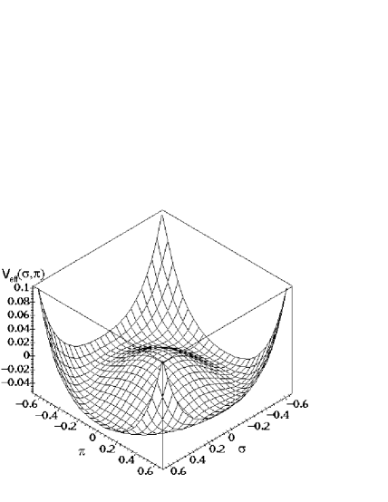
Figure 2: Vacuum structure for $\beta>\beta_{\pi}$. We see that the ground state is twice degenerate in the $\sigma_{0}$ direction while a false vacuum (or metastable vacuum) can be identified in the $\pi_{0}$ direction. After the identification of the true vacuum state we will no longer have a Goldstone boson.

$$\beta_{\sigma}^{2}=\frac{1}{24}\frac{\left(4\tilde{\lambda}-{\tilde{g}}^{2}\right)}{\tilde{m}^{2}}$$ (35)

and

$$\beta_{\pi}^{2}=\frac{1}{24}\frac{\left(4\tilde{\lambda}+{\tilde{g}}^{2}\right)}{\tilde{m}^{2}}.$$ (36)

Now, let us show that associated to each critical temperature there is a second order phase transition and a symmetry restoring phase. Indeed, if we go from zero temperature $(\beta=\infty)$ to a temperature close to $\beta_{\pi}^{-1}$ the effective potential takes the form of (fig. 2). There is a discrete degeneracy of the vacuum showing that in the previous section we made a correct choice of the ground-state.

If we continue increasing the temperature in such a way that $\beta_{\sigma}<\beta<\beta_{\pi}$ we note (see fig. 3) that the discrete symmetry in the $\pi_{0}$ direction is restored but we continue with a broken phase in the $\sigma_{0}$ direction. Complete restoration of symmetry (fig. 4) will only be achieved when $\beta<\beta_{\sigma}$, and this is exactly the picture after dimensional reduction since we have already taken the limit $\beta\rightarrow 0$.

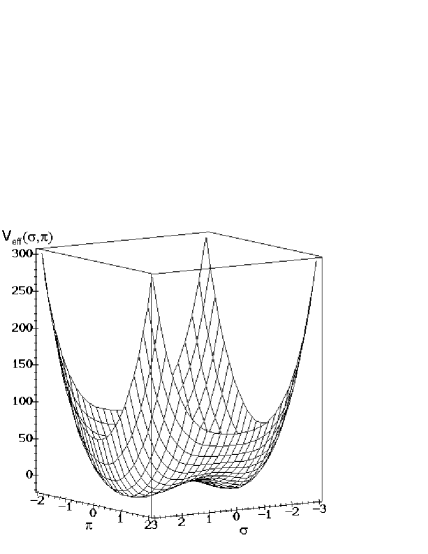
Figure 3: Partial restoration of symmetry for $\beta_{\sigma}<\beta<\beta_{\pi}$. The $\pi_{0}$ degree of freedom is now in the disordered phase while we still have discrete breakdown of symmetry in the $\sigma_{0}$ direction.

All the above discussion is valid only if $4\tilde{\lambda}>\tilde{g}^{2}$. What happens when $4\tilde{\lambda}<\tilde{g}^{2}$? In this case we will have only the $\beta_{\pi}$ critical temperature. This is to say, the discrete symmetry on the $\pi_{0}$ direction will be restored while, in the $\sigma_{0}$ direction, the minimum will become deeper and deeper as we increase the temperature. We will not have a complete restoration of symmetry and the effective potential will have the shape of (fig. 3).

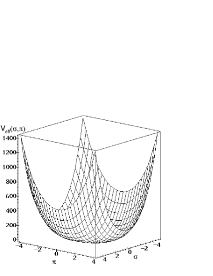
Figure 4: Complete disorder for $\beta<\beta_{\sigma}$. We see that, due to the difference in the thermal masses of the static fields $\sigma_{0}$ and $\pi_{0}$ this surface cannot be obtained by the revolution of a generating curve.

6 Conclusions

Dimensional reduction of the chiral-continous Gross-Neveu model was performed giving an effective theory that belongs to the same universality class of the Heisenberg magnet. In spite of the integration over fermions and nonstatic bosons modes have given mean field results for the critical indices, we were able to explicitely determine the universality class of the reduced theory by simply taking into account the effects of the only relevant degrees of freedom in the computation of thermodynamic quantities; the static Matsubara modes.

The presence of a coupling $i\gamma_{S}$ in the original action is the responsible for the difference on the thermal contributions for the masses of the pseudo-scalar and scalar fields $\sigma_{0}$ and $\pi_{0}$. This difference has important implications. First, we saw that if $4\tilde{\lambda}>\tilde{g}^{2}$ we have restoration of symmetry for some critical temperature, first in the $\pi_{0}$ direction and after in the $\sigma_{0}$ direction, while, if $4\tilde{\lambda}<\tilde{g}^{2}$ we have only partial restoration of symmetry. The introduction of temperature in a theory with a continous chiral symmetry has changed the role played by the $\pi_{0}$ field from the zero temperature case, where it was a Goldstone boson, to the finite-temperature case, where this is no longer true.

7 Acknowledgment

We are greatfull to C. de Callan, S. A. Dias and R. O. Ramos for interesting discussions. This paper was suported by Conselho Nacional de Desenvolvimento Científico e Tecnológico do Brasil (CNPq) and Fundação Coordenadoria de Aperfeiçoamento de Pessoal de Nível Superior (CAPES).

Appendix A - Thermal RG flow

We compute, for completeness, the thermal renormalization group functions which controlls the dependence of the counterterms on the temperature. As it is well known [12], the transition from a four-dimensional theory to an effective three-dimensional one is renormalization point dependent. This is not surprising since the Appelquist-Carazone decoupling theorem [6] only holds if a particular class of renormalization prescriptions is adopted, being optimal in BPHZ subtractions at zero momenta and temperature $\beta$. Neverthless, we can write down the thermal renormalization group equation which controls the dependence with the temperature on the correlation functions and compute the running quantities.

The independence of bare correlation functions on the choice of the renormalization point, is expressed by the conditions

$$\mu\frac{d}{d\mu}\Gamma^{(N)}=0,$$ (37)

$$T\frac{d}{dT}\Gamma^{(N)}=0,$$ (38)

and, for simplicity, we will work, in this section, with the temperature $T$ instead of $\beta\equiv 1/T$.

Since we are only interested on the computation of thermal renormalization group functions, we will consider solely

$$\left(T_{0}\frac{\partial}{\partial T_{0}}+\beta_{T}\frac{\partial}{\partial\lambda}+\gamma_{T}m^{2}\frac{\partial}{\partial m^{2}}\right)\Gamma^{(N)}=0$$ (39)

where

$$\beta_{T}=T_{0}\frac{\partial\lambda(T)}{\partial T_{0}},$$ (40)

$$\gamma_{T}=m^{-2}T_{0}\frac{\partial m^{2}(T)}{\partial T_{0}},$$ (41)

and

$$\Gamma^{(N)}=\left.\frac{\partial^{N}V_{\mbox{eff}}}{\partial\sigma_{0}^{N}}\right|_{\sigma_{0}=0}.$$ (42)

Using for the effective potential the expression (27) we easily get

$$\beta_{T}=\frac{1}{16\pi^{2}}\left(\frac{5}{12}\tilde{\lambda}^{2}+\tilde{g}^{4}\right),$$ (43)

and

$$\gamma_{T}=\frac{1}{12}\left(4\tilde{\lambda}-\tilde{g}^{2}\right)\frac{T^{2}}{m^{2}}+\frac{\tilde{\lambda}}{4\pi^{2}}.$$ (44)

Equation (39) can be solved by the method of characteristics. One simply introduces a dilatation parameter $t$ and look for functions $\lambda(t)$ (for fixed $g$) which satisfies

$$t\frac{d\lambda(t)}{dt}=\beta(\lambda(t)),$$ (45)

with $\lambda(1)=\lambda$. If we now solve the above equation we get

$$\int_{\lambda}^{\lambda(t)}\frac{d\lambda^{{}^{\prime}}}{\beta(\lambda^{{}^{\prime}})}=ln{t}.$$ (46)

To investigate the large $T$ limit we will have to study the behavior of the effective coupling $\lambda(t)$ as $t$ goes to zero. Since $\beta(\lambda)$ is positive $\lambda(t)$ will decrease. Moreover, since the slope of the $\beta$ function is also positive, the gaussian IR fixed point is attractive.

We can solve a similar equation to $g$ and defining $(\lambda^{*},g^{*})$ as the zero of the $\beta$ function

$$\beta(\lambda^{*},g^{*})=0,$$ (47)

we see that, although the anomalous dimension for the $\sigma_{0}$ field may change when we pass from the situation of total to the situation of partial restoration of symmetry, the $\eta$ exponent defined as $\eta\equiv\eta(\lambda^{*},g^{*})$ remains unchanged $(\eta=0)$.

One may ask whether renormalization group improves the critical indices after dimensional reduction or not. The answer is no and this should not be surprising since the form of the ultraviolet and thermal divergences that we had to renormalize are of the same type as for a theory in four dimensions, where everything is mean field.

References

- [1] G. Gat, A. Kovner and B. Rosenstein, Nucl. Phys. B385, 76 (1992).
- [2] B. Svetitsky and L. Yaffe, Nucl. Phys. B210, 423 (1982).
- [3] T. Appelquist and R. Pisarski, Phys. Rev. D 23, 2305 (1981); A. N. Jourjine, Ann. Phys. 155, 305 (1984); S. Nadkarni, Phys. Rev. D 27, 917 (1983); 38, 3287 (1988).
- [4] R. Pisarski and F. Wilczek, Phys. Rev. D 29, 338 (1984); F. Wilczek, Int. J. Mod. Phys. A 7, 3911 (1992); K. Rajagopal and F. Wilczek, Nucl. Phys. B404, 57 (1993); A. Bochkarev and J. Kapusta, Phys. Rev. D 54, 4066 (1996).
- [5] E. Braaten, Phys. Rev. Lett. 74, 2164 (1995); E. Braaten and A. Nieto, Phys. Rev. Lett. 76, 1417 (1996);
- [6] T. Appelquist and J. Carazone, Phys. Rev. D 11, 2856 (1975).
- [7] D. Amit, in Renormalization Group and Critical Phenomenon (World Scientific, Singapore, 1984); C. Itzykson and J. M. Drouffe, in Statistical Field Theory (Cambridge University Press, N.Y., 1989), vol. 1.
- [8] D. Gross and A. Neveu, Phys. Rev. D 10, 3235 (1974).
- [9] Y. Nambu and G. Jona-Lasinio, Phys. Rev. 122, 345 (1961).
- [10] E.S.Abers and B.W.Lee, Phys. Rep. 9, 1 (1973); B. Rosenstein, B. Warr and S. Park, Phys. Rep. 205, 59 (1991).
- [11] J. Zinn-Justin, Nucl. Phys. B367, 105 (1991).
- [12] N. P. Landsman, Nucl. Phys. B322, 498 (1989); E. Braaten and A. Nieto, Phys. Rev. D 51, 6990 (1995).
- [13] E. Elisalde and A. Romeo, J. Math. Phys. 30, 5 (1989).
- [14] A. P. C. Malbouisson, M. B. Silva-Neto and N. F. Svaiter, Physica A, to appear (1998).
- [15] B. Rosenstein, B. J. Warr and S. H. Park, Phys. Rev. D 39, 3088 (1989).
- [16] G. Gat et al., Phys. Lett. B 240, 158 (1990); A. N. Vasil’ev et al., Teor. Mat. Fiz. 92, 486 (1992); 94, 179 (1993); Saclay Report No. T96/016, (unpublished).
- [17] A. Kocić and J. Kogut, Phys. Rev. Lett. 74, 3110 (1995).
- [18] B. Rosenstein, A. D. Speliotopoulos and H. L. Yu, Phys. Rev. D 49, 6822 (1994).