Symmetries of Large $N_{c}$ Matrix Models for Closed Strings

Abstract

We obtain the symmetry algebra of multi-matrix models in the planar large $N_{c}$ limit. We use this algebra to associate these matrix models with quantum spin chains. In particular, certain multi-matrix models are exactly solved by using known results of solvable spin chain systems.

Quantum systems whose degrees of freedom are matrices appear in several areas of mathematics and physics; for example, Yang-Mills theory [1], [2], [3], [4], string theory[5], [6] and $M$ -theory[7], [8]. Of particular interest is the limit as the dimension $N_{c}$ of the matrices goes to infinity. In this limit the dynamics is expected to simplify; for example, the quantum fluctuations of the invariants are of order $1/N_{c}$ . The algebra of invariant observables becomes a Poisson algebra discovered in Ref.[9]. For the general large $N_{c}$ limit, these Poisson brackets are very non-linear. The planar large $N_{c}$ limit is equivalent to a further approximation that replaces this Poisson algebra with a Lie algebra. In this paper we will describe this Lie algebra of observables of the matrix model in the planar limit, by a direct argument.

As an illustration of the power of this new symmetry algebra, we will use it to solve some matrix models in the large $N_{c}$ limit. More precisely, we will map certain matrix models to quantum spin chains and use results from the theory of spin chains to solve them. This is reminiscent of the work [5] that connects some integrals over finite chains of matrices with classical integrable systems. From this point of view, our result is that certain path integrals over matrices can be mapped into quantum integrable systems. However we will mostly use the canonical formulation rather than the path integral formulation of these systems.

We will study a class of matrix models whose degrees of freedom are a set of matrix-valued bosonic variables $a^{\mu}_{\nu}(i),a^{{\dagger}\mu}_{\nu}(i)$ satisfying the canonical commutation relations $[a^{\mu}_{\nu}(i),a^{\rho}_{\sigma}(j)]=[a^{{\dagger}\mu}_{\nu}(i),a^{{\dagger}\rho}_{\sigma}(j)]=0$ and $[a^{\mu}_{\nu}(i),a^{{\dagger}\rho}_{\sigma}(j)]=\delta(i,j)\delta^{\mu}_{\sigma}\delta^{\rho}_{\nu}.$ Here, $\mu,\nu=1,2,\ldots$ or $N_{c}$ . The positions of the indices indicate the transformation properties under $U(N_{c})$ : $a^{\mu}_{\nu}\rightarrow g^{\mu}_{\rho}g^{*\sigma}_{\nu}a^{\rho}_{\sigma}$ etc. The degree of freedom labelled by the indices $\mu,\nu$ etc. will be called ‘color’ in analogy with quantum chromodynamics (QCD). Indeed our matrix model can be thought of as a regularized version of pure QCD, with the variables $a,a^{{\dagger}}$ representing gluons. The indices $i=1,\cdots,{\Lambda}$ describe the degrees of freedom (other than color) of the system. The Hamiltonian (along with all other observables) will be required to be color invariant, i.e., invariant under the adjoint action of $U(N_{c})$ on $a$ and $a^{{\dagger}}$ .

The path integral over matrix-valued functions of time, $P^{\mu}_{\nu}(j,t),Q^{\mu}_{\nu}(j,t)$ with Lagrangian

$$L(P,Q)=\sum_{j=1}^{{\Lambda}}P^{\mu}_{\nu}(j,t){d\over dt}Q^{\nu}_{\mu}(j,t)-H(P(t),Q(t))$$ (1)

gives an equivalent theory, with the identifications $a^{\mu}_{\nu}(j)=Q^{\mu}_{\nu}(j)+iP^{\mu}_{\nu}(j),a^{\mu{\dagger}}_{\nu}(j)=Q^{\mu}_{\nu}(j)-iP^{\mu}_{\nu}(j)$ ; but the canonical formulation is more convenient for our purposes.

Define the vacuum state of the representation of these relations by $a|0>=0$ . In the limit of large $N_{c}$ the color invariant states of the system are the ‘closed string’ (or ‘glueball’) states such as

$$\Psi^{(K)}=N_{c}^{-c/2}a^{\dagger\mu_{1}}_{\mu_{2}}(k_{1})a^{\dagger\mu_{2}}_{\mu_{3}}(k_{2})\cdots a^{\dagger\mu_{c}}_{\mu_{1}}(k_{c})|0\rangle.$$ (2)

Here strings of indices are denoted by capital letters. For example, $K$ stands for $k_{1},\cdots,k_{c}$ . The state is invariant under cyclic permutations; the equivalence class of permutations related to $K$ by cyclic permutations is denoted by $(K)$ .

The operators that dominate the large $N_{c}$ limit are

$$g^{I}_{J} \equiv N_{c}^{-(a+b-2)/2}a^{\dagger\mu_{1}}_{\mu_{2}}(i_{1})a^{\dagger\mu_{2}}_{\mu_{3}}(i_{2})\cdots a^{\dagger\mu_{a}}_{\nu_{b}}(i_{a})$$ (4)

$$a_{\nu_{b-1}}^{\nu_{b}}(j_{b})a_{\nu_{b-2}}^{\nu_{b-1}}(j_{b-1})\cdots a_{\mu_{1}}^{\nu_{1}}(j_{1}).$$

(Notice the reversal of order in the indices in the string $J$ ; this definition serves to simplify some later equations.) All observables of a matrix model which survive in the large $N_{c}$ limit– the Hamiltonian of regularized QCD for example – are linear combinations of such operators. These states and operators were previously studied in Ref. [2], where an elegant application to large $N_{c}$ QCD is described .

The factors of $N_{c}$ have been chosen to obtain the ‘planar’ limit; it is so called because in perturbation theory, the Feynman diagrams that survive can be drawn on a plane. There are other ways of taking the large $N_{c}$ limit, but the planar limit is the simplest.

In the limit as $N_{c}\to\infty$ these operators will map single closed string states to linear combinations of single closed string states (“glueballs”) :

$$g^{I}_{J}\Psi^{(K)}=\delta^{K}_{(J)}\Psi^{(I)}+\sum_{K_{1}K_{2}=(K)}\delta^{K_{1}}_{J}\Psi^{(IK_{2})}.$$ (5)

This is the key simplification of the planar limit. (To higher orders in the $1/N_{c}$ expansion, there will be terms that correspond to splitting a glueball into several glueballs.) Here, $\delta^{K}_{(J)}$ is equal to the number of different cyclic permutations of $J$ such that each permuted sequence is identical to $K$. Also, in the second term we sum over all ways of splitting the sequence $(K)$ into non-empty subsequences $K_{1}$ and $K_{2}$ . A graphical representation of  (5) is given in Fig. 1.

The operators $g^{I}_{J}$ are like matrices except that they operate on the space of cyclically symmetric tensors. We will call them ‘cyclix’ operators. The product $g^{I}_{J}g^{K}_{L}$ of two of the above operators is not a finite linear combination of the $g$ ’s themselves. But the commutator is indeed such a finite linear combination: finite linear combinations of the operators $g^{I}_{J}$ form a Lie algebra. (By finite linear cobinations we mean a sum over all sequences of indices $I$ and $J$ , of the form $\sum c^{J}_{I}g^{I}_{J}$ , such that only a finite number of the coefficients $c^{J}_{I}$ are non-zero.) The discovery of this Lie algebra is our main result. We will see that it has powerful consequences: for example we can solve some matrix models exactly using this newly discovered dynamical symmetry.

Before we describe the commutation relations between two $g^{I}_{J}$ ’s , it is convenient to introduce another kind of operator $\tilde{f}^{(I)}_{(J)}$ on closed string states. The defining equation for these operators is $\tilde{f}^{(I)}_{(J)}\Psi^{(K)}=\delta^{K}_{(J)}\Psi^{(I)}.$ These are thus the Weyl matrices in the basis $\Psi^{(I)}$ of closed string states up to constant multiples. Rather than being independent operators, they are in fact just linear combinations of $g^{I}_{J}$ : $\tilde{f}^{(I)}_{(J)}=g^{I}_{J}-\sum_{k=1}^{{\Lambda}}g^{Ik}_{Jk}$ and $\tilde{f}^{(I)}_{(J)}=g^{I}_{J}-\sum_{k=1}^{{\Lambda}}g^{kI}_{kJ}.$ The two different ways of writing $\tilde{f}^{(I)}_{(J)}$ imply that the operators $g^{I}_{J}$ are not linearly independent.

Now we can state the commutation relations of our Lie algebra:

$$\left[g^{I}_{{J}},g^{K}_{{L}}\right]=\delta^{K}_{J}g^{I}_{{L}}+\sum_{J_{1}J_{2}=J}\delta^{K}_{J_{2}}g^{I}_{{J_{1}L}}+\sum_{K_{1}K_{2}=K}\delta^{K_{1}}_{J}g^{IK_{2}}_{{L}}$$ (23)

$$+\sum_{\begin{array}[]{l}J_{1}J_{2}=J\\ K_{1}K_{2}=K\end{array}}\delta^{K_{1}}_{J_{2}}g^{IK_{2}}_{{J_{1}L}}+\sum_{J_{1}J_{2}=J}\delta^{K}_{J_{1}}g^{I}_{{LJ_{2}}}+\sum_{K_{1}K_{2}=J}\delta^{K_{2}}_{J}g^{K_{1}I}_{{L}}$$

$$+\sum_{\begin{array}[]{l}J_{1}J_{2}=J\\ K_{1}K_{2}=K\end{array}}\delta^{K_{2}}_{J_{1}}g^{K_{1}I}_{{LJ_{2}}}+\sum_{J_{1}J_{2}J_{3}=J}\delta^{K}_{J_{2}}g^{I}_{{J_{1}LJ_{3}}}$$

$$+\sum_{K_{1}K_{2}K_{3}=K}\delta^{K_{2}}_{J}g^{K_{1}IK_{3}}_{{L}}+\sum_{\begin{array}[]{l}J_{1}J_{2}=J\\ K_{1}K_{2}=K\end{array}}\delta^{K_{1}}_{J_{2}}\delta^{K_{2}}_{J_{1}}\tilde{f}^{(I)}_{({L})}$$

$$+\sum_{\begin{array}[]{l}J_{1}J_{2}J_{3}=J\\ K_{1}K_{2}=K\end{array}}\delta^{K_{1}}_{J_{3}}\delta^{K_{2}}_{J_{1}}\tilde{f}^{(I)}_{({J_{2}L})}+\sum_{\begin{array}[]{l}J_{1}J_{2}=J\\ K_{1}K_{2}K_{3}=K\end{array}}\delta^{K_{1}}_{J_{2}}\delta^{K_{3}}_{J_{1}}\tilde{f}^{(IK_{2})}_{({L})}$$

$$+\sum_{\begin{array}[]{l}J_{1}J_{2}J_{3}=J\\ K_{1}K_{2}K_{3}=K\end{array}}\delta^{K_{1}}_{J_{3}}\delta^{K_{3}}_{J_{1}}\tilde{f}^{(IK_{2})}_{({J_{2}L})}-(I\leftrightarrow K,J\leftrightarrow L).$$

Although it appears complicated when written this way, these commutation relations have a rather natural graphical interpretation which we will describe in a longer paper[10]. We will call the Lie algebra defined by these commutation relations the ‘cyclix Lie algebra’ or $\hat{\underline{C}}_{M}$ .

The above defined $\tilde{f}^{(I)}_{(J)}$ span an ideal of this algebra isomorphic to the inductive limit of linear algberas, $gl_{\infty}$ . ( $gl_{\infty}$ can also be defined as the Lie algebra of matrices with only a finite number of non-zero entries.)

We can quotient $\hat{\underline{C}}_{M}$ by this ideal to get another Lie algebra ${\underline{C}}_{M}$ , which is the essentially new object we have discovered. However it is only the extension $\hat{\underline{C}}_{M}$ that has a representation on the space of closed string states.

In the simplest special case of a matrix model with just one degree of freedom ( $M=1$ ), the algebra ${\underline{C}}_{1}$ is just the algebra of (polynomial) vector fields on the circle. $\hat{\underline{C}}_{1}$ is then the extension of this algebra by the algebra of finite-rank matrices[11]. Perhaps then ${\underline{C}}_{M}$ can be realized as the Lie algebra of vector fields on a non-commutative manifold.

We will now show how some large $N_{c}$ matrix models can be solved by using this new symmetry algebra. Suppose the Hamiltonian of a matrix model is a linear combination $H=\sum_{IJ}h^{J}_{I}g^{I}_{J}$ where $h^{J}_{I}=0$ unless $I$ and $J$ have the same number of indices. ( This means that the ‘gluon number’ is a conserved quantity: regularized QCD is not of this type.) Such linear combinations form a subalgebra; let us call it $\hat{\underline{C}}_{M}^{0}$ .

There is an isomorphism between multi-matrix models whose hamiltonians are in $\hat{\underline{C}}_{M}^{0}$ and quantum spin chains. Now, there are some well-known examples of exactly solved quantum spin chains; they yield exactly solved matrix models.

More explicitly, consider a spin chain with $\nu$ sites: at any site $a=1$ ,…, or $\nu$ , there is a variable $i_{a}$ (called ‘spin’ for historical reasons) that can take the value 1, 2, $\ldots$ , or ${\Lambda}$ . We will impose the periodic boundary condition. A basis of states is given by $|k_{1}\cdots k_{\nu}>.$

Define the operator

$$X^{i}_{j}(a)|k_{1}\cdots k_{\nu}>=\delta^{k_{a}}_{j}|k_{1}\cdots k_{a-1}ik_{a+1}\cdots k_{\nu}>.$$ (24)

This is just the Weyl matrix at site $a$ . Let $X^{i}_{j}(a)=X^{i}_{j}(a-\nu)$ if $a>\nu$. Now we can check that if $I$ and $J$ have the same length $b\leq\nu$ ,

$$r_{\nu}(g^{I}_{J})\equiv\sum_{a=1}^{\nu}X^{i_{1}}_{j_{1}}(a)X^{i_{2}}_{j_{2}}(a+1)\cdots X^{i_{b}}_{j_{b}}(a+b-1)$$ (25)

satisfies the commutation relations of the algebra $\hat{\underline{C}}^{0}_{M}$ . If we also set $r_{\nu}(g^{I}_{J})=0$ for $b>\nu$ , we will have a representation $r_{\nu}$ of $\hat{\underline{C}}^{0}_{M}$ . The states of the periodic spin chain with zero total momentum correspond to cyclically symmetric tensors which are the states of the matrix model.

With each matrix model whose hamiltonian $H=\sum_{IJ}h^{J}_{I}g^{I}_{J}$ is in $\hat{\underline{C}}^{0}_{M}$ , we can associate a quantum spin chain with the Hamiltonian

$$H^{\rm spin}=\sum_{IJ}h^{J}_{I}\sum_{a=1}^{\nu}X^{i_{1}}_{j_{1}}(a)X^{i_{2}}_{j_{2}}(a+1)\cdots X^{i_{b}}_{j_{b}}(a+b-1).$$ (26)

Thus matrix models conserving the gluon number correspond to quantum spin systems with interactions involving neighborhoods of spins $\{a,a+1,a+2,\ldots,a+b-1\}$ .

Let us look at some examples of solvable spin models and their associated matrix models. The simplest solvable quantum spin chain is perhaps the Ising model [12],[13]:

$$H^{\rm spin}_{\rm Ising}=\sum_{a=1}^{\nu}\tau^{z}(a)+\lambda\sum_{a=1}^{\nu}\tau^{x}(a)\tau^{x}(a+1).$$ (27)

Here $\tau^{x,y,z}_{a}$ are Pauli matrices at site $a$ . Let the states 1 and 2 in the matrix model correspond to the spin-up and spin-down states in the Ising model. Using the fact that $\tau^{z}_{a}=X^{1}_{1}(a)-X^{2}_{2}(a)$ and $\tau^{x}_{a}+i\tau^{y}_{a}=2X^{1}_{2}(j),$ we get the corresponding element in $\hat{\underline{C}}_{2}^{0}$ :

$$H^{\rm matrix}_{\rm Ising}=g^{1}_{1}-g^{2}_{2}+\lambda[g^{22}_{11}+g^{21}_{12}+g^{12}_{21}+g^{11}_{22}].$$ (28)

This is the large $N_{c}$ limit of the matrix model with the Hamiltonian

$$H^{\rm matrix}_{\rm Ising} = \;\;{\rm tr}\;\;[a^{{\dagger}}(1)a(1)-a^{{\dagger}}(2)a(2)]+{\lambda\over N_{c}}\;\;{\rm tr}\;\;[a^{{\dagger}}(2)a^{{\dagger}}(2)a(1)a(1)$$ (30)

$$+a^{{\dagger}}(2)a^{{\dagger}}(1)a(2)a(1)+a^{{\dagger}}(1)a^{{\dagger}}(2)a(1)a(2)+a^{{\dagger}}(1)a^{{\dagger}}(1)a(2)a(2)].$$

Our results, along with known results of the Ising spin chain [13] give the spectrum of this matrix model in the large $N_{c}$ limit:

$$E(n_{p},\nu)=-2\sum_{p=-\nu}^{\nu}\Bigg{(}1+2\lambda\cos\big{[}{2\pi p\over 2\nu+1}\big{]}+\lambda^{2}\Bigg{)}^{1/2}n_{p}$$ (31)

where $\nu$ is any positive integer and $n_{p}=0$ or 1. Also, we must impose the condition $\sum_{p=-\nu}^{\nu}n_{p}p=0$ to get cyclically symmetric states. In particular we see that the value $\lambda=1$ is the critical value of the matrix model at which the spectum (in the planar limit) is that of a massless free fermion field on a lattice.

It is interesting to ask whether the symmetries of the Ising spin chain can be understood within our formalism . Recall that [12],[14] the solvability of the Ising model is due to the existence of an infinite number of conserved quantities. They form an infinite-dimensional Lie algebra, the Onsager algebra. This is the Lie algebra generated by iterating commutators of two operators $H_{0}$ and $V$ satisfying $[H_{0},[H_{0},[H_{0},V]]]=16[H_{0},V]$ and $[V,[V,[V,H_{0}]]]=16[V,H_{0}].$ For the Ising model, $H_{0}=H=g^{1}_{1}-g^{2}_{2}$ and $V=g^{22}_{11}+g^{21}_{12}+g^{12}_{21}+g^{11}_{22}.$ Clearly, the Onsager algebra is a subalgebra of ${\underline{C}}_{M}^{0}$ . In particular, all conserved quantities of the Ising model are contained in our cyclix Lie algebra. It is not known whether this Ising matrix model is solvable for an arbitrary finite value of $N_{c}$ .

To every solved spin chain there is thus a corresponding solved matrix model. Instead of a comprehensive list, we are just going to give a few illustrative examples.

The generalization of the Ising model with the Hamiltonian [15]

$$H^{\rm spin}_{\rm GI}=\sum_{a=1}^{\nu}\tau^{z}_{a}+\lambda\sum_{a=1}^{\nu}[\tau^{x}_{a}\tau^{x}_{a+1}+v\{\tau^{x}_{a}\tau^{y}_{a+1}-\tau^{y}_{a}\tau^{x}_{a+1}\}]$$ (32)

also has the Onsager algebra as a dynamical symmetry. It corresponds to the element

$$H^{\rm matrix}_{\rm GI} = g^{1}_{1}-g^{2}_{2}+\lambda[g^{22}_{11}+(1-2iv)g^{21}_{12}+(1+2iv)g^{12}_{21}+g^{11}_{22}]$$ (33)

of the cyclix Lie algebra and hence to the exactly solvable matrix model

$$H^{{\rm matrix}}_{{\rm GI}} = \;\;{\rm tr}\;\;[a^{{\dagger}}(1)a(1)-a^{{\dagger}}(2)a(2)]+{\lambda\over N_{c}}\;\;{\rm tr}\;\;[a^{{\dagger}}(2)a^{{\dagger}}(2)a(1)a(1)$$ (36)

$$+(1-2iv)a^{{\dagger}}(2)a^{{\dagger}}(1)a(2)a(1)+(1+2iv)a^{{\dagger}}(1)a^{{\dagger}}(2)a(1)a(2)$$

$$+a^{{\dagger}}(1)a^{{\dagger}}(1)a(2)a(2)].$$

The XYZ model[16] with the Hamiltonian

$$H^{{\rm spin}}_{{\rm XYZ}}=\sum_{a=1}^{\nu}\tau^{z}_{a}\tau^{z}_{a+1}-\lambda\sum_{a=1}^{\nu}[\tau_{a}^{x}\tau^{x}_{a+1}+v\tau^{y}_{a}\tau^{y}_{a+1}]$$ (37)

is a generalization of the Ising model in another direction. The corresponding element in the cyclix algebra is

$$H^{{\rm matrix}}_{{\rm XYZ}}=g^{11}_{11}-g^{12}_{12}-g^{21}_{21}+g^{22}_{22}-\lambda[(1-v)(g^{22}_{11}+g^{11}_{22})+(1+v)(g^{21}_{12}+g^{12}_{21})].$$ (38)

A special case of this, the equivalence of a matrix model to the XXZ model, was found in [17].

The above correspondence between spin chains and matrix models is not restricted to the case ${\cal M}=2$ . The chiral Potts model [18] has the Hamiltonian

$$H^{{\rm spin}}_{{\rm CP}}=\sum_{a=1}^{\nu}\sum_{k=1}^{{\Lambda}-1}[\tilde{\alpha}_{k}Q_{a}^{k}+\lambda\alpha_{k}P_{a}^{k}P^{{\Lambda}-k}_{a+1}]$$ (39)

where $\alpha_{k},\tilde{\alpha}_{k}$ are constants. Also, $P_{a}$ and $Q_{a}$ are generalized spin matrices at site $a$ : $Q=\;{\rm diag}\;\;\big{(}1,\omega,\omega^{2},\cdots\omega^{{\Lambda}-1}\big{)}$ and $P$ is defined by $PQ=\omega QP$ . Here, $\omega=e^{2\pi i/{\Lambda}}$ . This model is exactly solvable and corresponds to the element

$$H^{{\rm matrix}}_{{\rm CP}}=\sum_{k=1}^{{\Lambda}-1}[\tilde{\alpha}_{k}\sum_{j=1}^{\nu}\omega^{k(j-1)}g^{j}_{j}+\lambda\alpha_{k}\sum_{j_{1},j_{2}=1}^{\nu}g^{j_{1}+k,\;j_{2}-k}_{j_{1}j_{2}}]$$ (40)

where $j_{1}+k$ should be replaced with $j_{1}+k-\Lambda$ if $j_{1}+k>\Lambda$ and $j_{2}-k$ should be replaced with $j_{2}+\Lambda-k$ if $j_{2}-k\leq 0$ in $g^{j_{1}+k,j_{2}-k}_{j_{1}j_{2}}$ of the cyclix algebra.

The problem of finding the partition function of the spectrum of a hamiltonian $H$ is equivalent to evaluating the path integral over paths of period $T$ : $\;\;{\rm Tr}\;\;e^{-iHT}=\int D[P]D[Q]e^{i\int_{0}^{T}[\sum_{j}\;\;{\rm tr}\;\;P(j)\dot{Q}(j)-H(P(j),Q(j))]dt}.$ where $H(P,Q)$ is obtained by substituting $a=Q+iP,a^{{\dagger}}=Q-iP$ into $H$ as described previously. By applying this transcription to the above systems, we can obtain path integrals over matrices which can be evaluated exactly in the planar large $N_{c}$ limit. We wont give explicit expressions to keep the paper short.

In addition to integrable matrix models associated with quantum spin chain models, we have also formulated models for QCD in terms of elements of the cyclix algebra [10]. We have also found the analog of the cyclix algebra suitable for studying open strings (‘meson states’) [19]; the supersymmetric extension has also been constructed [20]. The former is of interest in spin chains with open boundary conditions and QCD with quarks, and the latter in $M$ -theory.

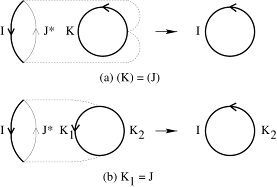
FIG. 1.: The action of a gluonic operator on a single glueball state. The gluonic operator $g^{I}_{J}$ searches for a substring of $K$ that agrees with $J$ . If found, it replaces each such substring with $I$ ; otherwise, we get zero. Here, $J^{*}$ denotes the reverse of the sequence $J$ .

REFERENCES

[1] G. ’t Hooft, Nucl. Phys. B 75, 461 (1974);
E. Brezin, C. Itzykson, G. Parisi and J. B. Zuber, Comm. Math. Phys. 59, 35 (1978);
E. Witten, Nucl. Phys. B 160, 57 (1979);
B. Sakita, Quantum Theory of Many-Variable Systems and Fields, Singapore: World Scientific
(World Scientific Lecture Notes in Physics: 1) (1985).
[2] C. B. Thorn, Phys. Rev. D 20, 1435 (1979).
[3] S. G. Rajeev, Phys. Letts B 209 53 (1988); Syracuse 1989, Proc., 11th Annual
Montreal-Rochester-Syracuse-Toronto Meeting, p.78;
Phy. Rev. D 42 2779 (1990); Phy. Rev. D 44 1836 (1991).
[4] K. Demeterfi, I. R. Klebanov and G. Bhanot, Nucl. Phys. B 418, 15 (1994);
F. Antonuccio and S. Dalley, Nucl. Phys. B 461, 275
(1996).
[5] M. R. Douglas, Phys. Lett. B 238, 176, (1990);
[6] O. Bergman and C. B. Thorn, Phys. Rev. D 52, 5980 (1995) and
Phys. Rev. Lett. 76, 2214 (1996).
[7] U. H. Danielsson, G. Ferretti and B. Sundborg, Int. J. Mod. Phys. A 11, 5463 (1996);
D. Kabat and P. Pouliot, Phys. Rev. Lett. 77, 1004 (1996).
[8] T. Banks, W. Fischler, S. H. Shenkar and L. Susskind, Phys. Rev. D 55, 5112 (1997);
L. Susskind, e-print hep-th/9704080.
[9] S. G. Rajeev and O. T. Turgut, J. Math. Phys. 37, 637 (1996).
[10] C.-W. H. Lee and S. G. Rajeev, to be published.
[11] V. G. Kac and D. H. Peterson, in Lectures on the Infinite Wedge-Representation and the MKP
Hierarchy,
Système dynamiques non lińeaires: intégrabilité et comportement qualitatif,
Sem. Math. Sup. 102, (Press Univ. Montréal, Montreal, Que. 1986).
[12] L. Onsager, Phys. Rev. 65, 117 (1944);
E. Fradkin and L. Susskind, Phys. Rev. D 17, 2637 (1978).
[13] J. B. Kogut, Rev. Mod. Phys. 51, 659 (1979).
[14] L. Dolan and M. Grady, Phys. Rev. D 25, 1587 (1982);
B. Davies, J. Math. Phys. 32, 2945 (1991).
[15] A. Honecker, Ph.D. thesis [e-print hep-th/9503104].
[16] R. J. Baxter, Exactly Solved Models in Statistical
Mechanics, Academic Press, London (1982).
[17] I. R. Klebanov and L. Susskind, Nucl. Phys. B 309, 175 (1988).
[18] H. Au-Yang, B. M. McCoy, J. H. H. Perk, S. Tang and M. L. Yan,
Phys. Lett. A 123, 219 (1987);
H. Au-Yang, R. J. Baxter and J. H. H. Perk, Phys. Lett. A 128 138 (1988);
Ph. Christe and M. Henkel,
Introduction to Conformal Invariance and its Applications to Critical Phenomena,
Lecture Notes in Physics m16 (Springer-Verlag, 1993).
[19] C.-W. H. Lee and S. G. Rajeev, e-print hep-th/9712090.
[20] C.-W. H. Lee and S. G. Rajeev, to be published.