Abstract

We study field theories in the limit that a compactified dimension becomes lightlike. In almost all cases the amplitudes at each order of perturbation theory diverge in the limit, due to strong interactions among the longitudinal zero modes. The lightlike limit generally exists nonperturbatively, but is more complicated than might have been assumed. Some implications for the matrix theory conjecture are discussed.

1 Introduction

Matrix theory [1] is a promising proposal for the fundamental degrees of freedom and Hamiltonian of M-theory. The further proposal [2] of Susskind, which gives a physical interpretation to the finite-$N$ matrix model, appears to be a major step forward. This proposal states that

$$\mbox{Finite $N$ matrix model}\ =\ \mbox{Discrete light cone quantization of M-theory}.$$ (1.1)

The left-hand side of this equation has a precise definition in terms of supersymmetric quantum mechanics, at least when the transverse dimensions are noncompact. It is the meaning of the right-hand side that we wish to address.

Discrete light cone quantization (DLCQ) [3] refers to compactification on a light-like circle,

$$(x^{+},x^{-},x^{i})\cong(x^{+},x^{-}+2\pi R,x^{i})\ ,$$ (1.2)

with fixed nonzero $p_{-}=n/R$. For the purpose of the conjecture (1.1), we believe that this must be understood as a limit of compactification on spacelike circles. This point of view has also been taken in some very recent papers [4]-[9].

We should note that most of the literature on DLCQ is not directed toward the above conjecture, but toward providing an infrared regulator for light-cone quantized field theories. In this case the discrete theory has no physical significance of its own, and the only physical criterion it must satisfy is to give the correct infinite volume limit. But for conjecture (1.1) to be meaningful, the right-hand side must have a natural and unique definition, and the limiting procedure provides this. If instead the DLCQ of M-theory is something different, the conjecture loses much of its content and becomes more of a definition. Further, it implies that matrix theory has a whole new moduli space of vacua, the discrete light-cone vacua, disconnected from all previously known moduli spaces. We think that this is unlikely to be true.

If our interpretation of the conjecture is correct, it raises a curious point. The finite-$N$ matrix theory is interpreted as one more limit of M-theory. But we already know many limits of M-theory: the various string theories, and eleven-dimensional supergravity. Why should one more limit generate great excitement? Presumably the answer is that while matrix theory is a limit of M-theory, it is hoped that the full M-theory can also be obtained as a limit of matrix theory, namely the limit of large $N$: taking $N\to\infty$ at fixed $R$ is Lorentz-equivalent to taking $R\to\infty$ holding the frame of an experiment fixed.

In this paper we will address not the second limiting procedure but the first: does it make sense to put a quantum system in a light-like box, in the limiting sense that we assume? Our study in this paper is limited to quantum field theory, rather than string or M-theory. The purpose is in part to develop some intuition in this simpler setting, but it is also of interest in its own right. Lightlike compactification is one of the few limits in which field theories dramatically simplify, and therefore is a tool that should be developed further.

We find that the situation is somewhat complicated. If we consider perturbation theory, the limit of lightlike compactification does not exist. That is, individual Feynman graphs diverge due to the infamous zero modes. In retrospect the problem is rather obvious. The zero modes are described by a field theory in one fewer dimension, interacting with fixed degrees of freedom representing the particles with nonzero $p_{-}$. We are holding fixed the parameters in the higher dimensional theory, so the coupling $g^{2}$ of the reduced theory scales as $R_{s}^{-1}$ with $R_{s}$ being the invariant length of the compact dimension. One would therefore expect every loop graph to diverge. The only theories that have smooth limits order-by-order are certain supersymmetric theories where the zero modes interact with the fixed degrees of freedom but not with each other.

However, if we consider the full theory, then it is likely that the limit does exist, at least if the original field theory itself exists in the sense of being asymptotically free in the ultraviolet. The lightlike limit is governed by an infrared fixed point, and in simple cases the zero modes simply become massive and cause no further trouble. While the limit appears to exist in most cases, our work points up the fact that it is more complicated than expected.

We should note that there are various discussions of zero modes in the DLCQ literature, for example the recent paper [10]. However, because the orthodox interpretation of DLCQ differs from ours, there seems to be little relation between the treatments of the zero modes. In particular, the standard DLCQ appears to treat them essentially classically.

Although our work is not specifically applicable to M-theory, we include in the conclusion some further discussion of recent work.

2 Scalar Field Theory

We start with a complex scalar field theory in $d$ dimensions with quartic self-interaction. We will denote the time coordinate by $\tau$, the periodic coordinate by $x^{-}$, and the remainder by $x^{i}$ for $i=3,\ldots,x^{d}$. The metric and periodicity are

$$ds^{2} = -2d\tau dx^{-}+\epsilon^{2}dx^{-}dx^{-}+dx^{i}dx^{i}\ ,$$

$$(\tau,x^{-},x^{i}) \cong (\tau,x^{-}+2\pi R,x^{i})\ .$$ (2.1)

The invariant length of the compact dimension is

$$R_{s}=2\pi\epsilon R\ .$$ (2.2)

The time $\tau$ is related to light-cone time $x^{+}$ by

$$\tau=x^{+}+\frac{\epsilon^{2}}{2}x^{-}\ ,$$ (2.3)

becoming identical in the limit $\epsilon\to 0$.

The action is

$$S=-\int d^{d}x\left(\partial_{\mu}\phi^{*}\partial^{\mu}\phi+M^{2}\phi^{*}\phi+\frac{g^{2}}{4}(\phi^{*}\phi)^{2}\right)\ .$$ (2.4)

We leave $d$ unspecified; a perturbatively well-defined theory requires $d\leq 4$, a nonperturbatively well-defined theory $d\leq 3$.

Expanding

$$\phi(\tau,x^{-},x^{i})=(2\pi R)^{-1/2}\sum_{n=-\infty}^{\infty}\phi_{n}(\tau,x^{i})e^{inx^{-}/R}\ ,$$ (2.5)

the kinetic term is

$$\sum_{n=-\infty}^{\infty}\int d\tau\,d^{d-2}x^{i}\left(\epsilon^{2}\partial_{\tau}\phi_{n}^{*}\partial_{\tau}\phi^{\vphantom{x}}_{n}+\frac{2in}{R}\phi_{n}^{*}\partial_{\tau}\phi^{\vphantom{x}}_{n}-\partial_{i}\phi_{n}^{*}\partial_{i}\phi^{\vphantom{x}}_{n}-M^{2}\phi^{*}\phi\right)\ .$$ (2.6)

This gives the propagator

$$\frac{i}{\epsilon^{2}p_{\tau}^{2}+2np_{\tau}/R-p_{i}p_{i}-M^{2}}\ =\ \frac{i}{\epsilon^{2}p_{\omega}^{2}-n^{2}/\epsilon^{2}R^{2}-p_{i}p_{i}-M^{2}}\ ,$$ (2.7)

where $p_{\omega}\equiv p_{\tau}+n/\epsilon^{2}R$.

Now consider the one loop amplitude in figure 1,

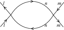
Figure 1: One loop scalar graph. Lines are labeled by $p_{-}R$, flowing in the direction of the arrow. The dangerous term is $n=0$.

$$\frac{g^{4}}{4\pi^{2}R^{2}}\sum_{n=-\infty}^{\infty}\int\frac{dq_{\tau}d^{d-2}q_{i}}{(2\pi)^{d-1}}$$ (2.8)

$$\qquad\Bigl{(}\epsilon^{2}q_{\omega}^{2}-n^{2}/\epsilon^{2}R^{2}-q_{i}q_{i}-M^{2}\Bigr{)}^{-1}\Bigl{(}\epsilon^{2}q^{\prime 2}_{\omega}-n^{2}/\epsilon^{2}R^{2}-q^{\prime}_{i}q^{\prime}_{i}-M^{2}\Bigr{)}^{-1}\ .$$

Here $q^{\prime}_{\mu}=q_{\mu}+k_{\mu}$, where $k_{\mu}$ is the exchanged momentum. We have taken the dangerous case $k_{-}=0$. The problematic term is $n=0$, where both lines in the loop have vanishing longitudinal momenta. When $\epsilon=0$, the integrand is independent of $q_{\tau}$ and the integral diverges. The integral is proportional to $\epsilon^{-1}$ and diverges in the limit of lightlike compactification.

One way to understand this is in coordinate space. In the lightlike limit of $\epsilon=0$, the kinetic term (2.6) for the zero modes has no $x^{+}$ (time) derivative and so the propagator is proportional to $\delta(x^{+})$. A closed loop of zero modes then involves $\delta(x^{+})^{2}\propto\delta(0)$. We can also understand the divergence from dimensional reduction. The effective loop expansion parameter in the dimensionally reduced zero mode theory is

$$g^{\prime 2}=\frac{g^{2}}{2\pi R\epsilon}\ .$$ (2.9)

Leaving the external lines fixed and summing over all graphs with internal zero mode lines reproduces the full complication of the dimensionally reduced field theory, interacting with fixed sources representing the external lines. In the lightlike limit the coupling in this theory diverges.

Now let us examine the case $d=3$, where the original theory is weakly coupled in the UV and should exist nonperturbatively. The effective dimensionless coupling at length $l$ in the zero mode theory is $g^{2}l^{2}/R\epsilon$. At the cutoff distance $l=R\epsilon$ this actually goes to zero in the lightlike limit, so the theory should be well-defined. However, it diverges at any fixed $l$. In fact, one expects a mass gap at

$$l\approx\epsilon^{1/2}R^{1/2}/g$$ (2.10)

where the effective coupling becomes strong. Thus the zero mode dynamics cures itself: at any fixed distance, the zero modes decouple when $\epsilon$ is taken to zero. However, amplitudes with vanishing $p_{-}$ exchange will be very different from their form in the noncompact theory, due to the gap.

This same kind of analysis should apply to any theory that is asymptotically free in the UV, such as four dimensional nonsupersymmetric or supersymmetric gauge theory. If the IR fixed point has massless fields, then some residue of the zero mode dynamics will survive.

Finally let us remark on the $n\neq 0$ terms in the amplitude (2.8). At large $\epsilon$ these take the form

$$\frac{ig^{4}\epsilon^{2}R}{16\pi^{2}n^{3}}\int\frac{d^{d-2}q_{i}}{(2\pi)^{d-2}}(1+\epsilon^{2}q_{i}q_{i}R^{2}/n^{2})^{-3/2}\ .$$ (2.11)

At fixed $q_{i}$ this vanishes as $\epsilon\to 0$, consistent with the analysis of Weinberg [11]: for either time-ordering of the vertices in figure 1, there is a particle with negative $p_{-}$. The integrated amplitude also vanishes in $d<4$, but in $d=4$ it scales as $\epsilon^{0}$. Further it is proportional to $n^{-1}$ so the sum diverges. This just reflects the fact that the nonzero modes renormalize the coupling to the scale $R_{s}$.

3 The $+-0$ Model

In the course of this investigation we did find one theory whose light-cone limit is finite order-by-order. This is a toy model inspired by our eventual interest in $N=4$ gauge theories. It is a supersymmetric model with three chiral superfields and superpotential

$$W=g\Phi^{+}\Phi^{-}\Phi^{0}\ .$$ (3.1)

We also introduce nondynamical ‘Wilson lines,’, so that the compact momenta for $\Phi^{\pm}$ are shifted,

$$p_{-}=\frac{r}{R}\ ,\quad r\in{\bf Z}\pm\nu\ .$$ (3.2)

Here $\nu$ is an arbitrary noninteger constant. The point is that the fields in $\Phi^{\pm}$ do not have zero modes, so the effective zero mode theory is free.

The absence of divergences is still nontrivial, because the zero modes interact with the external states.

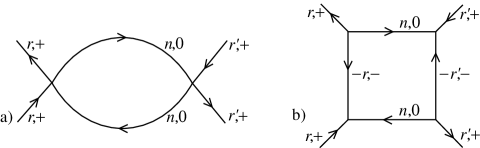
Figure 2: a) A divergent scalar graph. Lines are labeled by $p_{-}R$ and by the superfield. Other divergent graphs are obtained by replacing a pair of $+$ superfields with $-$. b) Canceling fermion loop.

Thus figure 2a has the same divergence as figure 1. Now, however, it is canceled by the fermion loop of figure 2b. More generally, any closed loop of bosonic zero modes, generalizing figure 2a to $2M$ external lines, will give one net $\delta(0)$. The divergence is canceled by a corresponding fermion loop.

Rather than show the graphical calculations explicitly we give an argument based on supersymmetry. The zero mode theory lives at a single light-cone time, so to first approximation we can ignore the $x^{+}$-dependence of the external lines. The supersymmetry transformations that close on translation of $x^{+}$ are then unbroken by the external lines, and guarantee net vanishing of the loop amplitude (again, to leading order in $\epsilon$).

Let us see this explicitly. We write out in components the relevant terms in the Lagrangian, using the conventions and notations of Wess and Bagger [12], except that we denote scalars by $\phi$:

$${\cal L} = -\,\epsilon^{2}\partial_{\tau}\phi_{0}^{*}\partial_{\tau}\phi_{0}^{\vphantom{x}}-\partial_{i}\phi_{0}^{*}\partial_{i}\phi^{\vphantom{x}}_{0}-i\bar{\psi}_{0}\left(\bar{\sigma}^{+}\partial_{\tau}+\mbox{$\frac{1}{2}$}\epsilon^{2}\bar{\sigma}^{-}\partial_{\tau}+\bar{\sigma}^{i}\partial_{i}\right)\psi_{0}$$ (3.3)

$$-\,i\bar{\psi}_{r}\left(\bar{\sigma}^{+}\partial_{\tau}+\mbox{$\frac{1}{2}$}\epsilon^{2}\bar{\sigma}^{-}\partial_{\tau}+i\bar{\sigma}^{-}rR^{-1}+\bar{\sigma}^{i}\partial_{i}\right)\psi_{r}$$

$$-\,2\Lambda_{r}\psi_{-r}\psi_{0}-{\rm h.c.}-4\Lambda^{*}_{r}\Lambda^{\vphantom{x}}_{r}\phi_{0}^{*}\phi^{\vphantom{x}}_{0}\ .$$

We have kept only fields that contribute to the loop graphs. In particular, the scalars with nonzero $p_{-}$ do not appear, but the fermions with nonzero $p_{-}$ appear in figure 2b. All terms are quadratic in the quantum fields. We have adopted a rather condensed notation. The subscript labeling the superfields is omitted, because the $p_{-}$ moding is sufficient to distinguish these. The index $r$ runs over the values (3.2) for both $\pm\nu$, thus implying also a sum over the superfields $\pm$. The coupling and backgrounds are joined in

$$\Lambda_{r}=g\phi_{r}\ .$$ (3.4)

To make the $\epsilon\to 0$ limit clear we redefine $\tau=\epsilon t$, and make a Lorentz boost on the spinor indices so that

$$\sigma^{+}\to\epsilon\sigma^{+}\ ,\quad\sigma^{-}\to\epsilon^{-1}\sigma^{-}\ .$$ (3.5)

The Lagrangian becomes

$${\cal L} = -\,\partial_{t}\phi_{0}^{*}\partial_{t}\phi_{0}^{\vphantom{x}}-\partial_{i}\phi_{0}^{*}\partial_{i}\phi^{\vphantom{x}}_{0}-i\bar{\psi}_{0}\left(\bar{\sigma}^{+}\partial_{t}+\mbox{$\frac{1}{2}$}\bar{\sigma}^{-}\partial_{t}+\bar{\sigma}^{i}\partial_{i}\right)\psi_{0}$$ (3.6)

$$-\,i\bar{\psi}_{r}\left(\bar{\sigma}^{+}\partial_{t}+\mbox{$\frac{1}{2}$}\bar{\sigma}^{-}\partial_{t}+i\epsilon^{-1}\bar{\sigma}^{-}rR^{-1}+\bar{\sigma}^{i}\partial_{i}\right)\psi_{r}$$

$$-\,2\Lambda_{r}\psi_{-r}\psi_{0}-{\rm h.c.}-4\Lambda^{*}_{r}\Lambda^{\vphantom{x}}_{r}\phi_{0}^{*}\phi^{\vphantom{x}}_{0}\ .$$

The action acquires an overall $\epsilon$ from $d\tau$, which implies the loop counting factor of $\epsilon^{-1}$. Otherwise, $\epsilon$ appears only in one term, where it causes one component of $\psi_{r}$ to decouple. The surviving component, designated by a prime, satisfies

$$\bar{\sigma}^{-}\psi^{\prime}_{r}=0\ ,\quad\sigma^{-}\bar{\sigma}^{+}\psi^{\prime}_{r}=2\psi^{\prime}_{r}\ .$$ (3.7)

The Lagrangian finally comes to the form

$${\cal L} = -\,\partial_{t}\phi_{0}^{*}\partial_{t}\phi_{0}^{\vphantom{x}}-\partial_{i}\phi_{0}^{*}\partial_{i}\phi^{\vphantom{x}}_{0}-i\bar{\psi}_{0}\left(\bar{\sigma}^{+}\partial_{t}+\mbox{$\frac{1}{2}$}\bar{\sigma}^{-}\partial_{t}+\bar{\sigma}^{i}\partial_{i}\right)\psi_{0}$$ (3.8)

$$-\,i\bar{\psi}^{\prime}_{r}\bar{\sigma}^{+}\partial_{t}\psi^{\prime}_{r}-\,2\Lambda^{\vphantom{x}}_{r}\psi^{\prime}_{-r}\psi^{\vphantom{x}}_{0}-{\rm h.c.}-4\Lambda^{*}_{r}\Lambda^{\vphantom{x}}_{r}\phi_{0}^{*}\phi^{\vphantom{x}}_{0}\ .$$

To leading order in $\epsilon$, the background is invariant under the supersymmetry whose parameter $\xi^{\prime}$ satisfies (3.7). Correspondingly the action (3.8) is invariant under

$$\delta\phi_{0} = \sqrt{2}\xi^{\prime}\psi_{0}\ ,$$

$$\delta\psi_{0} = \sqrt{2}i\sigma^{i}\bar{\xi}^{\prime}\partial_{i}\phi_{0}+i\sqrt{2}\sigma^{+}\bar{\xi}^{\prime}\partial_{t}\phi_{0}\ ,$$

$$\delta\psi^{\prime}_{r} = -2\sqrt{2}\xi^{\prime}\Lambda_{-r}^{*}\phi_{0}^{\vphantom{x}}\ .$$ (3.9)

This acts linearly on the quantum fields, and so guarantees cancellation of the leading $\epsilon^{-1}$ term in the one loop amplitude.

4 Discussion

Our work points out that for rather simple dimensional reasons, the limit of lightlike compactification leads to a strong coupling problem in almost any field theory. This may reduce the promise of this idea as a means of studying field theory dynamics: DLCQ is not a free lunch.

To conclude, we comment on some very recent papers on matrix theory, in particular one that seems to derive the matrix model [5] and one [6] that seems to show that it is incorrect. Other very recent papers [7, 8, 9] discuss related issues.

Roughly speaking, the recent paper by Seiberg [5] observes that compactification on a nearly lightlike circle is Lorentz-equivalent to compactification on a circle of small spacelike radius $R_{s}$. The latter compactification of M-theory gives the IIA string, but now in a sector with nonzero D0-brane charge $p_{-}=n/R$. Taking $R_{s}\to 0$ while holding distances fixed in units of the eleven-dimensional Planck scale, one retains just the open string ground states, which are indeed described by the matrix theory. This approach allows one to understand the increase in the number of degrees of freedom when several coordinates are periodically identified, from additional light states that survive the limiting process. Similar arguments are made by Sen [7].

Dine and Rajaraman [6] calculate a three-graviton to three-graviton process in eleven-dimensional supergravity and obtain a result that is not in agreement with the corresponding two-loop matrix theory calculation. Is this in direct contradiction with the derivation in ref. [5]? Does the argument in that paper actually imply the previous successful tests of matrix model scattering, and therefore that the matrix model and supergravity calculations in ref. [6] must agree? We do not see why this should be so. The established range of validity for the supergravity calculation is eleven large dimensions, while the derivation of the matrix theory deals with M-theory compactified on a circle small compared to the eleven-dimensional Planck scale. Without some additional physical input, mere boosts of coordinate systems and uniform rescaling of units of length will not turn one regime into the other.

We could try to provide the additional input as follows. Consider the supergravity scattering process in eleven large dimensions, but in a frame (which can always be chosen for few enough particles) where the $p_{-}$ components are integer multiples of some length $R$, assumed to be greater than the eleven-dimensional Planck length. One could then consider the same process in a spacetime with the null identification (1.2). Actually let us consider first an identification that is almost null, with invariant periodicity $R_{s}$ much less than the Planck scale, and then take a limit. By the argument in ref. [5], the resulting physics is indeed described by the matrix theory Hamiltonian. The one nontrivial step would then seem to be the periodic identification: should we expect this to leave the amplitude invariant?

It is certainly not obvious that this should be so. One effect of the compactification is that loop momenta are quantized, leading as we have seen to strong coupling effects. The compactified theory then breaks down at longer distance, the ten-dimensional rather than eleven-dimensional Planck scale. A second effect is the introduction of winding sectors, in this case winding membranes which are IIA strings (this point is also made in ref. [8]). This causes supergravity to break down at even longer distance, the string scale. This is just the point that the supergravity description is valid for small $R_{s}$ but distances large compared to the string scale, while the matrix theory description is valid for small $R_{s}$ and distances small compared to the string scale.

Thus, while the scaling argument of Seiberg shows that the conjecture (1.1) is literally true, it does not explain the agreement with supergravity calculations, guarantee that future supergravity calculations will agree or enable us to reconstruct the eleven-dimensional limit. For the same reason, the paper [4], which purported to test the conjecture (1.1), does not. Rather, it tests some not yet clearly formulated assumption about continuation from the supergravity regime to the matrix theory regime.

Additional input, perhaps the large-$N$ limit, is needed. Note that even at large $N$ the zero modes become strongly coupled as $R_{s}\to 0$, so it is necessary to show that these decouple from the large-$N$ process.

Acknowledgments

We would like to thank Melanie Becker, Katrin Becker, Shanta de Alwis, Michael Dine, Eric Gimon, David Gross, Juan Maldacena, Hirosi Ooguri, Nati Seiberg, and Charles Thorn for discussions and communications. This work was supported in part by NSF grants PHY94-07194 and PHY97-22022.

References

- [1] T. Banks, W. Fischler, S. H. Shenker and L. Susskind, Phys. Rev. D55 (1997) 5112, hep-th/9610043.
- [2] L. Susskind, Another Conjecture about M(atrix) Theory, Stanford preprint, hep-th/9704080.
-
[3]
T. Maskawa and K. Yamawaki, Prog. Theor. Phys. 56 (1976) 270;
A. Casher, Phys. Rev. D14 (1997) 452;
R. Giles and C. B. Thorn, Phys. Rev. D16 (1977) 366;
C. B. Thorn, Phys. Rev. D19 (1979) 639;
H. C. Pauli and S. J. Brodsky, Phys. Rev. D32 (1985) 1993, 2001. - [4] K. Becker, M. Becker, J. Polchinski, and A. Tseytlin, Phys. Rev. D56 (1997) 3174, hep-th/9706072.
- [5] N. Seiberg, Why is the Matrix Model Correct? IAS preprint, hep-th/9710009.
- [6] M. Dine and A. Rajaraman, Multigraviton scattering in the matrix model, Santa Cruz/SLAC preprint, hep-th/9710174.
- [7] A. Sen, D0-Branes on and Matrix Theory, Mehta preprint, hep-th/9709220.
- [8] M. R. Douglas and H. Ooguri, Why Matrix Theory is Hard, IHES/LBL/Rutgers/Berkeley preprint, hep-th/9710178.
- [9] S. P. de Alwis, Matrix Models and String World Sheet Duality, IAS preprint, hep-th/9710219.
- [10] K. Yamawaki, Zero Mode and Symmetry Breaking on the Light Front, Nagoya preprint, hep-th/9707141.
- [11] S. Weinberg, Phys. Rev. 150 (1966) 1313.
- [12] J. Wess and J. Bagger, “Supersymmetry and Supergravity,” Princeton, Princeton University Press, 1992.
- [13] O. J. Ganor, R. Gopakumar, and S. Ramgoolam, Higher Loop Effects in M(atrix) Orbifolds, preprint hep-th/9705188.