Gonihedric String Equation I

We discuss the basic properties of the gonihedric string and the problem of its formulation in continuum. We propose a generalization of the Dirac equation and of the corresponding gamma matrices in order to describe the gonihedric string. The wave function and the Dirac matrices are infinite-dimensional. The spectrum of the theory consists of particles and antiparticles of increasing half-integer spin lying on quasilinear trajectories of different slope. Explicit formulas for the mass spectrum allow to compute the string tension and thus demonstrate the string character of the theory. The string tension varies from trajectory to trajectory and indicates nonperturbative character of the spectrum. Additional $\Gamma_{5}$ and pure Casimir mass terms in the string equation allow to increase the slope of the trajectories, so that the mass spectrum grows as $j^{3}$ and $j^{5}$. The equation does not admit tachyonic solutions, but still has unwanted ghost solutions. We include bosons and show that they also lie on the same quasilinear trajectories.

1 Introduction

There is some experimental and theoretical evidence for the existence of a string theory in four dimensions which may describe strong interactions and represent the solution of QCD [6].

One of the possible candidates for that purpose is the gonihedric string which has been defined as a model of random surfaces with an action which is proportional to the linear size of the surface [7]

$$A(M_{2})=m\sum_{<ij>}\lambda_{ij}\cdot\Theta(\alpha_{ij}),~{}~{}~{}~{}~{}~{}~{}\Theta(\alpha)=|\pi-\alpha|^{\varsigma},$$ (1)

where $\lambda_{ij}$ is the length of the edge $<ij>$ of the triangulated surface $M_{2}$ and $\alpha_{ij}$ is the dihedral angle between two neighbouring triangles of $M$ sharing a common edge $<ij>$. The angular factor $\Theta$ defines the rigidity of the random surfaces [7]. The action has been defined for self-intersecting surfaces as well [7] and is equal to

$$A(M_{2})=m\sum_{<ij>}\lambda_{ij}\cdot\Theta(\alpha_{ij})~{}~{}+~{}~{}k_{r}~{}m\sum_{<ij>}\lambda_{ij}\cdot(\Theta(\alpha^{(1)}_{ij})+...+\Theta(\alpha^{(r)}_{ij}))$$ (2)

where the number of terms inside parentheses is equal to the order of the intersection $r=3,4,...$;  $r$ is the number of triangles sharing the edge $<ij>$. The coupling constant $k_{r}$ is called self-intersection coupling constant [13] .

The model has a number of properties which make it very close to the Feynman path integral for a point-like relativistic particle. This can be seen from (1) in the limit when the surface $M_{2}$ degenerates into a single world line $M_{1}$ (see Figure 9), in that case

$$A(M_{2})~{}~{}=~{}m\int_{M_{2}}(\frac{1}{R_{1}}+\frac{1}{R_{2}})~{}dS~{}~{}\rightarrow~{}2\pi m\int_{M_{1}}~{}dL~{}~{}=~{}~{}L(M_{1}).$$ (3)

In this limit the classical equation of motion for the gonihedric string

$$K~{}=~{}\frac{1}{R_{1}~{}R_{2}}~{}=~{}0,$$

which describes the evolution of rigid string, is reduced to the classical equation of motion for a free relativistic particle.

The other important property of the theory is that at the classical level the string tension is equal to zero and quarks viewed as open ends of the surface are propagating freely without interaction [7]:

$$\sigma_{classical}=0.$$

This is because the gonihedric action (1) is equal to the perimeter $P(M_{2})$ of the flat Wilson loop

$$A(M_{2})\rightarrow~{}~{}~{}~{}P(M_{2})=R+T$$

and the potential $V(R)$ is constant. As it was demonstrated in [7], quantum fluctuations generate the nonzero string tension

$$\sigma_{quantum}=\frac{d}{a^{2}}~{}(1-ln\frac{d}{\beta}),$$ (4)

where $d$ is the dimension of the spacetime, $\beta$ is the coupling constant, $a$ is the scaling parameter and $\varsigma=(d-2)/d$ in (1). In the scaling limit $\beta\rightarrow\beta_{c}=d/e$ the string tension has a finite limit while the scaling parameter tends to zero as $a=(\beta-\beta_{c})^{1/2},$ thus the critical exponent $\nu$ is equal to one half, $\nu=1/d_{H}=1/2$ , where $d_{H}$ is the Hausdorff dimension.

Thus at the tree level the theory describes free quarks with the string tension equal to zero, quantum fluctuations generate nonzero string tension and, as a result, the quark confinement [7]. The gonihedric string may consistently describe asymptotic freedom and confinement as it is expected to be the case in QCD and we have to ask what type of equation may describe this string. The aim of this article is to answer this question.

Some additional understanding of the physical behaviour of the system comes from the transfer matrix approach [14]. The transfer matrix can be constructed in two cases, $k=0$ and $k=\infty$, that is for $free-intersecting$ and $self-avoiding~{}surfaces$. In both cases it describes the propagation of the closed string $M^{\tau}_{1}$ in time direction $\tau$ with an amplitude which is proportional to the sum of the length of the string and of the total curvature [14]

$$A(M^{\tau}_{1})=\int_{M^{\tau}_{1}}dL+\int_{M^{\tau}_{1}}k(L)dL$$

and of the interaction which is proportional to the overlapping length of the string on two neighbouring time slices

$$A_{int}(M^{\tau};M^{\tau+1})=\int_{M^{\tau}\cap\ M^{\tau+1}}dL.$$

Considering the system of closed paths on a given time slice $\tau$ as a separate system with the length and curvature amplitude one can see that this two-dimensional system has a continuum limit which can be described by a free Dirac fermion [14]. Thus on every time slice the system generates a fermionic string which may propagate in time because of the week interaction between neighbouring time slices [14]. Thus the physical picture of the fermionic string propagation which follows from the transfer matrix approach again stresses the need for answering the question of the corresponding string equation.

In addition to the formulation of the theory in the continuum space the system allows an equivalent representation on Euclidean lattices where a surface is associated with a collection of plaquettes [12, 13]. Lattice spin systems whose interface energy coincides with the action (1) have been constructed in an arbitrary dimension $d$ [12] for the self-intersection coupling constant $k=1$ and for an arbitrary $k$ in [13]. This gives an opportunity for numerical simulations of the corresponding statistical systems in a way which is similar to the Monte Carlo simulations of QCD [16]. The Monte Carlo simulations [18] demonstrate that the gonihedric system with a large intersection coupling constant undergoes the second order phase transition and the string tension is generated by quantum fluctuations, as it was expected theoretically [7]. This result again suggests the existence of a noncritical string theory in four dimensions.

It is natural to think that each particle in this theory should be viewed as a state of a complex fermionic system and that this system should have a point-particle limit when there is no excitation of the internal motion, thus requiring the basic property of the gonihedric string (3). The question is then how to incorporate this internal motion into existing point particle equations. Ettore Majorana suggested in 1932 [2] an extension of the Dirac equation by constructing an infinite-dimensional representation of the Lorentz group and the corresponding extension of the gamma matrices. The equation has the Dirac form

$$\{~{}i~{}\Gamma_{\mu}~{}\partial^{\mu}~{}~{}-~{}~{}M~{}\}~{}~{}\Psi~{}~{}~{}=0$$ (5)

and the Majorana commutation relations which define the $\Gamma_{\mu}$ matrices are given by the formula (see (13) in [2])

$$[\Gamma_{\mu},~{}I_{\lambda\rho}]=\eta_{\mu\lambda}~{}\Gamma_{\rho}-\eta_{\mu\rho}~{}\Gamma_{\lambda},$$ (6)

where $I_{\mu\nu}$ are the generators of the Lorentz algebra. These equations allow to find the $\Gamma_{\mu}$ matrices when the representation of the $I_{\mu\nu}$ is given. The original Majorana solution for $\Gamma_{\mu}$ matrices is infinite-dimensional (see equation (14) in [2]) and the mass spectrum of the theory is equal to

$$M_{j}=\frac{M}{j+1/2},$$ (7)

where $j=1/2,3/2,5/2,....$ in the fermion case and $j=0,1,2,....$ in the boson case. The main problems in the Majorana theory are the decreasing mass spectrum (7), absence of antiparticles and troublesome tachyonic solutions - the problems common to high spin theories. Nevertheless we intend to interpret the Majorana theory as a natural way to incorporate $additional$ degrees of freedom into the relativistic Dirac equation. The problem is to formulate physical principles allowing to choose appropriate representations of the Lorentz group in order to have a string equation with necessary properties. The above discussion of the gonihedric string shows that an appropriate equation should exist. Indeed we shall demonstrate that the solution of the Majorana commutation relations exists and the corresponding equation has an increasing mass spectrum (10), (11) and nonzero string tension (8).

An alternative way to incorporate the internal motion into the Dirac equation was suggested by Pierre Ramond in 1971 [3]. In his extension of the Dirac equation the internal motion is incorporated through the construction of operator-valued gamma matrices. The equations which define the $\Gamma_{\mu}$ matrices are

$$<\Gamma_{\mu}(\tau)>=\gamma_{\mu},$$

$$\{\Gamma_{\mu}(\tau),\Gamma_{\nu}(\tau^{{}^{\prime}})\}=2\eta_{\mu\nu}~{}\delta(~{}\frac{1}{2\pi\alpha^{{}^{\prime}}}~{}(\tau-\tau^{{}^{\prime}})~{})$$

$$\Gamma^{+}_{\mu}(\tau)~{}\gamma_{0}=\gamma_{0}~{}\Gamma_{\mu}(\tau),$$

where it is required that the proper-time average $<...>$ over the periodic internal motion with period $2\pi\alpha^{{}^{\prime}}=1/\sigma$ should coincide with the Dirac matrices. The mass spectrum lies on the linear trajectories

$$M^{2}_{n}=\frac{1}{\alpha^{{}^{\prime}}}~{}(j+n-3/2)~{}~{}~{}~{}~{}~{}~{}~{}~{}~{}~{}~{}~{}n=1,2,3,....$$

where $\sigma$ is the string tension, $j=1/2,3/2,...$ and $n$ enumerates the trajectories (here part of the states are spurious). In both cases one can see effective extensions of Dirac gamma matrices into the infinite-dimensional case, but these extensions are quite different. The free Ramond string is a consistent theory in ten dimensions and the spectrum contains a massless ground state .

For our purposes we shall follow Majorana’s approach to incorporate the internal motion in the form of an infinite-dimensional wave equation. Unlike Majorana we shall consider the infinite sequence of high- dimensional representations of the Lorentz group with nonzero Casimir operators $(\vec{a}\cdot\vec{b})$ and $(\vec{a}^{2}-\vec{b}^{2})$. The important restriction which we have to impose on the system is that it should have a point particle limit. In the given case this restriction should be understood as a principle according to which the infinite sequence of representations should contain the Dirac spin one-half representation. In the next section we shall review the known representations of the Lorentz group $SO(3,1)$ and shall select necessary representations for our purpose. These representations $(j_{0},\lambda)$ and their adjoint $(j_{0},-\lambda)$ are enumerated by the index $r=j_{0}+1/2$, where $r=1,...,N$ and $j_{0}=1/2,3/2,...$  is the lower spin in the representation $(j_{0},\lambda)$, thus $j=j_{0},j_{0}+1,...$. The representations used in the Dirac equation are $(1/2,-3/2)$ and $(1/2,3/2)$ and in the Majorana equation they are $(0,1/2)$ in the boson case and $(1/2,0)$ in the fermion case. We shall introduce also the concept of the dual representation which is defined as $\Theta=(j_{0};\lambda)\rightarrow(\lambda;j_{0})=\Theta^{dual}$. This dual transformation is essentially used in subsequent sections to construct the solution of the Majorana commutation relations which has an increasing mass spectrum and is bounded from bellow.

The invariant Lagrangian, the string equation and the Majorana commutation relations are formulated in the third and forth sections. In the fifth and six sections the solution of Majorana commutators is constructed for small values $N=1,2,....$ in the form of Jacoby matrices [10] and then it is used to construct the solution for an arbitrary $N$. This basic solution (we shall call it $B$-solution) is well defined for any $N$ and allows to take the limit $N\rightarrow\infty$. The spectrum can be computed for any $N$ and demonstrates a tendency to concentrate around the eigenvalues $+1$ and $-1$. When $N\rightarrow\infty$ all masses are equal to one and the spectrum is bounded from bellow, but the $\Gamma_{0}$ matrix is not Hermitian. In the next four sections we reach the necessary Hermitian property of the system and the correct commutation relation with the matrix of the invariant form. The solution is symmetric and we shall call it $\Sigma$-solution. The spectrum of the theory now consists of particles and antiparticles of increasing half-integer spin and lying on quasilinear trajectories of different slope

$$2\pi\sigma_{n}=\frac{1}{\alpha^{{}^{\prime}}_{n}}=\frac{2M^{2}}{n}~{}~{}~{}~{}~{}~{}n=1,2,3....$$ (8)

here $n$ enumerates the trajectories and the lower spin on a trajectory is $j=n+1/2$. This result demonstrates that we have indeed a string equation which has trajectories with different string tension and that trajectories with large $n$ are almost ”free” because the string tension tends to zero. The number of particles with a given spin $j$ is equal to $j+1/2$. The components of the wave function which describe spin $j$ satisfy a partial differential equation of order $2j+1$. The corresponding differential operator is a sum of the powers of the D’Alembertian. The general formula for all trajectories is

$$M^{2}_{n}=\frac{2M^{2}}{n}~{}\frac{j^{2}-(2n-1)j+n(n-1)}{j-(n-1)/2}~{}~{}n=1,2,...$$

where $j=n+1/2,n+5/2,....$. The unwanted property of the $\Sigma$-solution is that the smallest mass on a given trajectory $n$ has the spin $j=n+1/2$ and decreases as $M^{2}_{n}(j=n+1/2)=3M^{2}/n(n+3)$,   the disadvantage which is common with the Majorana solution (7). In the eleventh section we introduce additional $(\vec{a}\cdot\vec{b})~{}\Gamma_{5}$ and pure Casimir $(\vec{a}^{2}-\vec{b}^{2})$ mass terms into the string equation (5)

$$\{~{}i~{}\Gamma_{\mu}~{}\partial^{\mu}~{}~{}-~{}~{}M~{}(\vec{a}\cdot\vec{b})\Gamma_{5}~{}~{}-~{}~{}gM~{}(\vec{a}^{2}-\vec{b}^{2})~{}\}~{}~{}\Psi~{}~{}~{}=0$$ (9)

where $(\vec{a}\cdot\vec{b})$ and $(\vec{a}^{2}-\vec{b}^{2})$ are the Casimir operators of the Lorentz algebra. These terms essentially increase the string tension so that all trajectories have a nonzero slope, but still we have a decreasing part in the spectrum.

The cardinal solution of the problem is given in the twelfth section where we perform a $dual$ transformation of the system. The dual formula for the mass spectrum is

$$M^{2}_{n}=\frac{2M^{2}}{n}~{}\frac{(j+n)(j+n+1)}{j+(n+1)/2},~{}~{}~{}~{}~{}~{}~{}~{}~{}~{}~{}~{}n=1,2,...$$ (10)

The lower spin on a given trajectory is either $1/2$ or $3/2$ depending on n: if n is odd then $j_{min}=1/2$, if n is even then $j_{min}=3/2$. The essentially new property of the dual equation is that now we have an infinite number of states with a given spin $j$ instead of $j+1/2$, which we had before we did the dual transformation. String tension has the same values as in (8) and the lower mass on a given trajectory $n$ is given by the formula $M^{2}_{n}(j=1/2)=4M^{2}(2n+1)(2n+3)/n(n+2)\rightarrow(4M)^{2}$ and the similar one for $M^{2}_{n}(j=3/2)$. Thus the main problem of decreasing spectrum has been solved after the dual transformation because the spectrum is now bounded from below. Additional $\Gamma_{5}$ mass term is also analyzed with the main result

$$M^{2}_{n}=\frac{2M^{2}}{n}\frac{(j+n)^{2}(j+n+1)^{2}}{j+(n+1)/2}\frac{1}{4}~{}~{}~{}~{}~{}n=1,2,...$$ (11)

and the pure Casimir mass term with the following spectrum

$$M^{2}_{n}=g^{2}~{}\frac{2M^{2}}{n}\frac{(j+n)^{3}(j+n+1)^{3}}{j+(n+1)/2}~{}~{}~{}~{}~{}n=1,2,3,...$$ (12)

In the last thirteenth section we extend the equation to include bosons and show that bosons also lie on the same quasilinear trajectories (10). At the end we discuss the problems of tachyonic and ghost solutions of the Majorana and of the new equation. Some technical details can be found in the Appendixes.

2 Representations of Lorentz Algebra

The algebra of the $SO(3,1)$ generators [11, 2]

$$[I^{\mu\nu}~{}I^{\lambda\rho}]=-\eta^{\mu\lambda}~{}I^{\nu\rho}+\eta^{\nu\lambda}~{}I^{\mu\rho}+\eta^{\mu\rho}~{}I^{\nu\lambda}-\eta^{\nu\rho}~{}I^{\mu\lambda}$$

can be rewritten in terms of $SO(3)$ generators $\vec{a}$ and Lorentz boosts $\vec{b}$

$$a_{x}=iI^{23}~{}~{}~{}~{}a_{y}=iI^{31}~{}~{}~{}~{}a_{z}=iI^{12}$$

$$b_{x}=iI^{10}~{}~{}~{}~{}b_{y}=iI^{20}~{}~{}~{}~{}b_{z}=iI^{30}$$

as [2] (we use Majorana’s notations)

$$[a_{x},a_{y}]=ia_{z}$$ (13)

$$[a_{x},b_{y}]=ib_{z}$$ (14)

$$[b_{x},b_{y}]=-ia_{z}.$$ (15)

The irreducible representations $R^{(j)}$ of $SO(3)$ algebra (13) are

$$<j,m|~{}a_{z}~{}|j,m>=m$$

$$<j,m|~{}a_{+}~{}|j,m-1>=\sqrt{(j+m)(j-m+1)}$$

$$<j,m|~{}a_{-}~{}|j,m+1>=\sqrt{(j+m+1)(j-m)},$$ (16)

where $m=-j,...,+j$,   the dimension of $R^{(j)}$ is   $2j+1$   and $j=0,~{}1/2,~{}1,~{}3/2,~{}...$ Then

$$<j,m|~{}\vec{a}^{2}~{}|j,m>=j(j+1).$$

Since $\vec{b}$ transforms as a vector under $SO(3)$ spatial rotations (14) it follows that

$$<j|~{}\vec{b}~{}|j^{\prime}>=0$$

unless $j^{\prime}=j$, or $j^{\prime}=j~{}\pm 1$, thus the matrix elements of $\vec{b}$ are fixed by their vector character, apart from the factors depending on $j$ but not on $m$. Therefore the solution of the commutation relations (14) for $\vec{b}$ can be parameterized as [11, 2]

$$<j,m|~{}b_{z}~{}|j,m>=\lambda_{j}\cdot m$$

$$<j-1,m|~{}b_{z}~{}|j,m>=\varsigma_{j}\cdot\sqrt{(j^{2}-m^{2})}$$

$$<j,m|~{}b_{z}~{}|j-1,m>=\varsigma_{j}\cdot\sqrt{(j^{2}-m^{2})}$$

$$<j,m|~{}b_{+}~{}|j,m-1>=~{}\lambda_{j}\cdot\sqrt{(j+m)(j-m+1)}$$

$$<j-1,m|~{}b_{+}~{}|j,m-1>=~{}\varsigma_{j}\cdot\sqrt{(j-m)(j-m+1)}$$

$$<j,m|~{}b_{+}~{}|j-1,m-1>=-\varsigma_{j}\cdot\sqrt{(j+m)(j+m-1)}$$

$$<j,m|~{}b_{-}~{}|j,m+1>=~{}\lambda_{j}\cdot\sqrt{(j-m)(j+m+1)}$$

$$<j-1,m|~{}b_{-}~{}|j,m+1>=-\varsigma_{j}\cdot\sqrt{(j+m)(j+m+1)}$$

$$<j,m|~{}b_{-}~{}|j-1,m+1>=~{}\varsigma_{j}\cdot\sqrt{(j-m)(j-m-1)}$$ (17)

where the amplitudes $\lambda_{j}$ describe diagonal transitions inside the $SO(3)$ multiplet $R^{(j)}$ while $\varsigma_{j}$ describe nondiagonal transitions between $SO(3)$ multiplets which form the representation $\Theta$ of $SO(3,1)$. These amplitudes should satisfy the boundary condition

$$(j_{0}+1)\lambda_{j_{0}}=i~{}\lambda~{}~{}~{}~{}~{}~{}~{}\varsigma_{j_{0}}=0,$$ (18)

where $j_{0}$ defines the lower spin in the representation $\Theta=(j_{0};\lambda)$ and $\lambda$ is a free parameter, thus

$$\Theta(j_{0},\lambda)=\oplus\sum^{\infty}_{j=j_{0}}~{}R^{(j)}.$$ (19)

The amplitudes $\lambda$ and $\varsigma$ can be found from the last of the commutation relations (15) rewritten in the component form

$$(2j+3)\cdot\varsigma^{2}_{j+1}-(2j-1)\cdot\varsigma^{2}_{j}-\lambda^{2}_{j}=1$$

$$\{(j+1)\cdot\lambda_{j}-(j-1)\cdot\lambda_{j-1}\}\cdot\varsigma_{j}=0.$$ (20)

From the last recursion equation and the boundary conditions (18) it follows that

$$\lambda_{j}~{}=~{}\frac{j-1}{j+1}~{}\lambda_{j-1}=~{}~{}\frac{j_{0}(j_{0}+1)}{j(j+1)}~{}\lambda_{j_{0}}=~{}~{}i\frac{j_{0}~{}\lambda}{j(j+1)},$$ (21)

where $j_{0}$ is the lower spin in the representation $\Theta=(j_{0};\lambda)$ and $\lambda$ appears as an essential dynamical parameter which cannot be determined solely from the kinematics of the Lorentz group. Substituting $\lambda_{j}$ from (21) into (20) one can find $\varsigma_{j}$

$$\varsigma^{2}_{j}=\frac{(~{}j^{2}-j^{2}_{0}~{})~{}(~{}j^{2}-\lambda^{2})}{j^{2}~{}(~{}4j^{2}-1~{})}$$ (22)

in terms of $j_{0}$ and $\lambda$. The adjoint representation is defined as $\dot{\Theta}=(j_{0};-\lambda)$ and we shall introduce here also the concept of the dual representation which we define as

$$\Theta=(j_{0};\lambda)\longleftrightarrow(\lambda;j_{0})=\Theta^{dual}$$ (23)

The representations used in the Dirac equation are $(1/2,-3/2)$ and $(1/2,3/2)$ and in the Majorana equation they are $(0,1/2)$ in the boson case and $(1/2,0)$ in the fermion case. The infinite-dimensional Majorana representation $(1/2,0)$ contains $j=1/2,3/2,...$ multiplets of the $SO(3)$ while $(0,1/2)$ contains $j=0,1,2,...$ multiplets. The essential difference between these representations is that the Lorentz boost operators $\vec{b}$ are diagonal in the first case ( the diagonal amplitudes (21) are $\lambda^{1}_{1/2}=-\lambda^{\dot{1}}_{1/2}=i$ and nondiagonal amplitudes (22) are equal to zero $\varsigma^{1}_{3/2}=\varsigma^{\dot{1}}_{3/2}=0$) and they are nondiagonal in the case of Majorana representations (the nondiagonal amplitudes are $\varsigma_{j}=1/2$ and the diagonal amplitudes are equal to zero $\lambda_{j}=0$ as it follows from (21) and (22) and coincide with the solution (19) in [2] ).

Let us consider pairs of adjoint representations with $j_{0}=1/2,~{}3/2,~{}\cdots$

$$\Theta_{r}=(j_{0};\lambda)~{}~{}~{}~{}~{}~{}~{}~{}~{}\Theta_{\dot{r}}=(j_{0};-\lambda)$$ (24)

which we shall enumerate by the representation index $r=1,2,3,...$    so that $j_{0}=r-1/2$ (see Fig.1). The corresponding matrices $\vec{b}^{r}$ and $\vec{b}^{\dot{r}}$ are defined by (17) where from (21) and (22) we have

$$\lambda^{r}_{j}=-\lambda^{\dot{r}}_{j}=i~{}\frac{r-1/2}{j(j+1)}~{}\lambda~{}~{}~{}~{}~{}~{}~{}~{}j\geq r-1/2$$ (25)

and

$$\varsigma^{r}_{j}=\varsigma^{\dot{r}}_{j}=\frac{1}{2}\sqrt{(1-\frac{r^{2}-r}{j^{2}-1/4})(1-(\frac{\lambda}{j})^{2})}~{}~{}~{}~{}~{}~{}j\geq r+1/2$$ (26)

and we shall consider the case when

$$-3/2\leq\lambda\leq 3/2$$ (27)

to have $\varsigma$ real for all values of $r$. The Casimir operators $(\vec{a}\cdot\vec{b})$ and $~{}(\vec{a}^{2}-\vec{b}^{2})~{}$ for the representation $\Theta_{r}$ are equal correspondingly to

$$<j,m|~{}\vec{a}\cdot\vec{b}~{}|j,m>=i~{}\lambda~{}(r-1/2)$$ (28)

$$<j,m|~{}(\vec{a}^{2}-\vec{b}^{2})~{}|j,m>=(r-1/2)^{2}+\lambda^{2}-1.$$ (29)

As it is easy to see from these formulas the Casimir operator $(\vec{a}\cdot\vec{b})$ is nonzero only if $\lambda\neq 0$. For the Majorana representations $(1/2,0)$ and $(0,1/2)$ the Casimir operator $(\vec{a}\cdot\vec{b})$ is equal to zero.

3 The Invariant form, Lagrangian and conserved current

To have an invariant scalar product

$$<~{}\Theta~{}\Psi_{1}~{}|~{}\Theta~{}\Psi_{2}~{}>~{}~{}~{}=~{}~{}~{}<~{}\Psi_{1}~{}|~{}\Psi_{2}~{}>$$ (30)

where $\Theta=1+\frac{1}{2}\epsilon_{\mu\nu}~{}I^{\mu\nu}$, one should define the matrix $\Omega$

$$<~{}\Psi_{1}~{}|~{}\Psi_{2}~{}>=\bar{\Psi}_{1}~{}\Psi_{2}=\Psi^{+}_{1}~{}\Omega~{}\Psi_{2}=\Psi^{*~{}r}_{1~{}jm}~{}\Omega^{rr^{\prime}}_{jm~{}j^{\prime}m^{\prime}}~{}\Psi^{r^{\prime}}_{2~{}j^{\prime}m^{\prime}}$$ (31)

with the properties

$$\Omega~{}a_{k}=a_{k}~{}\Omega$$ (32)

$$\Omega~{}b_{k}=b^{+}_{k}~{}\Omega$$ (33)

$$\Omega=\Omega^{+}.$$ (34)

From the first relation it follows that

$$\Omega=\omega^{rr^{\prime}}_{j}\cdot\delta_{jj^{\prime}}\cdot\delta_{mm^{\prime}}$$ (35)

and from the last two equations, for our choice of the representation $\Theta$ (24)-(27) and for a real $\lambda$,

$$\omega^{r\dot{r}}_{j}=\omega^{\dot{r}r}_{j}~{}=~{}1~{}~{}~{}\omega^{2}_{j}=1,$$ (36)

thus $\Omega$ is an antidiagonal matrix

$$\bar{\Psi}_{1}~{}\Psi_{2}~{}~{}=~{}~{}\sum^{\infty}_{r=1}~{}\sum^{\infty}_{j=r-1/2}\sum^{j}_{m=-j}~{}(~{}\Psi^{*~{}r}_{1~{}jm}~{}\Psi^{~{}\dot{r}}_{2~{}jm}+\Psi^{*~{}\dot{r}}_{1~{}jm}~{}\Psi^{~{}r}_{2~{}jm}~{})$$ (37)

and to have a finite invariant product the summation should be convergent .

Having in hand the invariant form (37) one can construct the Lagrangian

$$L=\int~{}\{i~{}\bar{\Psi}~{}\Gamma_{\mu}~{}\partial^{\mu}~{}\Psi~{}-i~{}\partial^{\mu}~{}\bar{\Psi}~{}\Omega\Gamma^{+}_{\mu}\Omega~{}\Psi~{}-2~{}M~{}\bar{\Psi}~{}\Psi~{}\}~{}d^{4}x$$ (38)

and the corresponding equation of motion

$$\{~{}i~{}(\Gamma_{\mu}+\Omega\Gamma^{+}_{\mu}\Omega)~{}\partial^{\mu}~{}~{}-~{}2~{}M~{}\}~{}~{}\Psi~{}~{}~{}=0.$$ (39)

Multiplying the conjugate equation

$$-i~{}\partial^{\mu}~{}\Psi^{+}~{}(\Omega\Gamma_{\mu}\Omega+\Gamma^{+}_{\mu})~{}-2M~{}\Psi^{+}~{}~{}=0$$ (40)

by $\Omega$ from the r.h.s. we have

$$-i~{}\partial^{\mu}~{}\bar{\Psi}~{}(\Gamma_{\mu}+\Omega\Gamma^{+}_{\mu}\Omega)~{}-2M~{}\bar{\Psi}~{}~{}=0$$ (41)

and then from both equations follows the conservation of the current

$$J_{\mu}=i~{}\bar{\Psi}~{}\frac{(\Gamma_{\mu}+\Omega\Gamma^{+}_{\mu}\Omega)}{2}~{}\Psi~{}~{}~{}~{}~{}~{}~{}~{}~{}\partial^{\mu}~{}J_{\mu}=0.$$ (42)

The crucial point is that current density should be positive definite

$$J_{0}=i~{}\Psi^{+}~{}\frac{(\Omega\Gamma_{0}+\Gamma^{+}_{0}\Omega)}{2}~{}\Psi,$$ (43)

which is equivalent to the positivity of the eigenvalues of the matrix

$$\rho=\frac{\Omega~{}\Gamma_{0}+\Gamma^{+}_{0}~{}\Omega}{2}.$$ (44)

If in addition the important relation is required to be satisfied

$$\Gamma^{+}_{\mu}~{}\Omega=\Omega~{}\Gamma_{\mu},$$ (45)

then the current will have the form

$$J_{\mu}=i~{}\bar{\Psi}~{}\Gamma_{\mu}~{}\Psi,$$ (46)

and equation (39) can be transformed in this case into Hamiltonian form

$$i~{}\frac{\partial~{}\Psi}{\partial~{}t}=H~{}\Psi$$ (47)

with the Hamiltonian

$$H=\Gamma^{-1}_{0}~{}\vec{\Gamma}~{}\vec{p}~{}+~{}\Gamma^{-1}_{0}~{}M.$$ (48)

4 Majorana commutation relations for Gamma matrices

The Lagrangian and the equation

$$\{~{}i~{}\Gamma_{\mu}~{}\partial^{\mu}~{}~{}-~{}~{}M~{}\}~{}~{}\Psi~{}~{}~{}=0$$ (49)

should be invariant under Lorentz transformations

$$X^{\prime}_{\mu}=\Lambda_{\mu}^{~{}\nu}~{}X_{\nu}~{}~{}~{}~{}~{}~{}~{}~{}~{}~{}\Psi^{\prime}(X^{\prime})=\Theta(\Lambda)~{}\Psi(X),$$ (50)

which leads to the following equation for the gamma matrices

$$\Gamma_{\nu}=\Lambda_{\nu}^{~{}\mu}~{}\Theta~{}\Gamma_{\mu}~{}\Theta^{-1}.$$ (51)

If we use the infinitesimal form of Lorentz transformations

$$\Lambda_{\mu\nu}=\eta_{\mu\nu}+\epsilon_{\mu\nu}~{}~{}~{}~{}~{}~{}~{}~{}\Theta=1+\frac{1}{2}\epsilon_{\mu\nu}~{}I^{\mu\nu}$$ (52)

it follows that gamma matrices should satisfy the Majorana commutation relation [2]

$$[\Gamma_{\mu},~{}I_{\lambda\rho}]=\eta_{\mu\lambda}~{}\Gamma_{\rho}-\eta_{\mu\rho}~{}\Gamma_{\lambda}$$ (53)

or in components (see formulas (13) in [2])

$$[\Gamma_{0},~{}a_{x}]=0~{}~{}~{}~{}~{}~{}[\Gamma_{0},~{}b_{x}]=i\Gamma_{x}$$ (54)

$$[\Gamma_{x},~{}a_{x}]=0~{}~{}~{}[\Gamma_{x},~{}a_{y}]=i\Gamma_{z}~{}~{}~{}[\Gamma_{x},~{}a_{z}]=-i\Gamma_{y}$$ (55)

$$[\Gamma_{x},~{}b_{x}]=i\Gamma_{0}~{}~{}~{}~{}~{}[\Gamma_{x},~{}b_{y}]=0~{}~{}~{}~{}~{}[\Gamma_{x},~{}b_{z}]=0~{}~{}~{}~{}$$ (56)

From these equations it follows that $\Gamma_{\mu}$ should satisfy the equation

$$[[\Gamma_{\mu},~{}b_{k}],~{}b_{k}]=-\Gamma_{\mu}~{}~{}~{}~{}~{}~{}~{}~{}~{}~{}~{}~{}k=x,y,z.$$ (57)

One can also derive that

$$\{\Gamma_{0}~{}\Gamma_{k}\}=i~{}[b_{k}~{}\Gamma^{2}_{0}],$$ (58)

thus the anticommutator between $\Gamma_{0}$ and $\Gamma_{k}$ essentially depends on the form of the $\Gamma^{2}_{0}$ operator. These are the most important equations because they allow to find gamma matrices when a representation $\Theta$ of the Lorentz algebra is given. It is an art to choose an appropriate representation $\Theta$ in order to have an equation with the necessary properties. We shall choose $N$ pairs of adjoint representations with $j_{0}=1/2,...,N-1/2$ (see Fig.1).

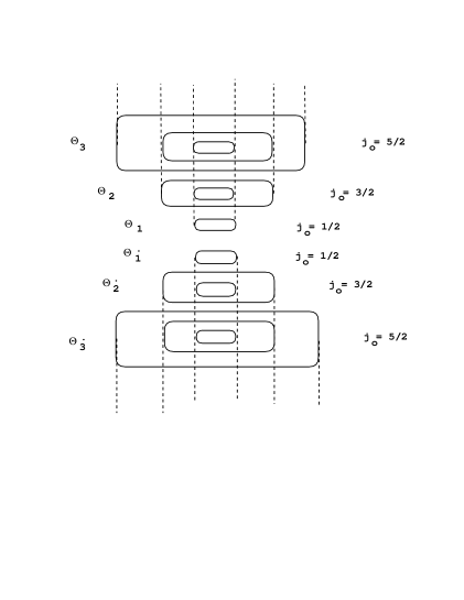
Figure 1: The tower of infinite-dimensional representations of Lorentz group $\Theta=(\Theta_{\dot{N}},\cdots,\Theta_{\dot{1}},\Theta_{1},\cdots,\Theta_{N})$. The number of states on the spin level j is equal to j+1/2.

Because $\Gamma_{0}$ commutes with spatial rotations $\vec{a}$ it should have the form

$$<j,m|~{}\Gamma^{rr^{\prime}}_{0}~{}|j^{\prime}m^{\prime}>=\gamma^{rr^{\prime}}_{j}\cdot\delta_{jj^{\prime}}\cdot\delta_{mm^{\prime}}~{}~{}~{}~{}~{}~{}~{}r,r^{\prime}=\dot{N},...,\dot{1},1,...,N$$ (59)

where we consider $N$ pairs of adjoint representations $\Theta=(\Theta_{\dot{N}},\cdots,\Theta_{\dot{1}},\Theta_{1},\cdots,\Theta_{N})$, thus $\gamma^{rr^{\prime}}$ is $2N\times 2N$ matrix which should satisfy the equation (57) for $\mu=0$ and the wave function has the form (see Fig.1)

$$\left(\begin{array}[]{c}\Psi^{r}_{jm}\\ \Psi^{\dot{r}}_{jm}\end{array}\right)~{}~{}~{}r=1,...,N~{}~{}~{}~{}~{}~{}j=r-1/2,~{}r+1/2,...~{}~{}~{}~{}~{}~{}~{}m=-j,...,j.$$ (60)

It should be understood that

$$\vec{a}^{~{}rr^{\prime}}=\delta^{rr^{\prime}}\cdot\vec{a}~{}~{}~{}~{}~{}~{}~{}~{}\vec{b}^{~{}rr^{\prime}}=\delta^{rr^{\prime}}\cdot\vec{b}^{~{}r}.$$ (61)

One can compute $\Gamma_{k}$ matrices using relation $\Gamma_{k}=i~{}(b_{k}~{}\Gamma_{0}~{}-~{}\Gamma_{0}~{}b_{k})$,  $k=x,y,z$

$$<j,m,r~{}|~{}\Gamma_{z}~{}|~{}r+1,j,m>=i~{}m~{}(\lambda^{r}_{j}-\lambda^{r+1}_{j})\cdot\gamma^{rr+1}_{j}$$

$$<j,m,r+1~{}|~{}\Gamma_{z}~{}|~{}r,j,m>=-i~{}m~{}(\lambda^{r}_{j}-\lambda^{r+1}_{j})\cdot\gamma^{r+1r}_{j}$$

$$<j-1,m,r~{}|~{}\Gamma_{z}~{}|~{}r+1,j,m>=i~{}\sqrt{j^{2}-m^{2}}\cdot(\varsigma^{r}_{j}\gamma^{rr+1}_{j}-\gamma^{rr+1}_{j-1}\varsigma^{r+1}_{j})$$

$$<j-1,m,r+1~{}|~{}\Gamma_{z}~{}|~{}r,j,m>=i~{}\sqrt{j^{2}-m^{2}}\cdot(\varsigma^{r+1}_{j}\gamma^{r+1r}_{j}-\gamma^{r+1r}_{j-1}\varsigma^{r}_{j})$$

$$<j,m,r+1~{}|~{}\Gamma_{z}~{}|~{}r,j-1,m>=-i~{}\sqrt{j^{2}-m^{2}}\cdot(\varsigma^{r}_{j}\gamma^{r+1r}_{j}-\gamma^{r+1r}_{j-1}\varsigma^{r+1}_{j})$$

$$<j,m,r~{}|~{}\Gamma_{z}~{}|~{}r+1,j-1,m>=-i~{}\sqrt{j^{2}-m^{2}}\cdot(\varsigma^{r+1}_{j}\gamma^{rr+1}_{j}-\gamma^{rr+1}_{j-1}\varsigma^{r}_{j}).$$ (62)

It is appropriate to introduce separate notations for diagonal and nondiagonal parts of $\Gamma_{k}$, we shall define them as $\tilde{\Gamma_{k}}$ and $\tilde{\tilde{\Gamma_{k}}}$.

We start by analyzing the situation for some lower values of $N$. A pattern emerges which is then used to construct the solution in the general case.

5 N pairs of infinite dimensional representations

5.1 N=1

First we shall consider the pair of infinite-dimensional adjoint representations $\Theta=(~{}\Theta_{\dot{1}},\Theta_{1}~{})$

$$\Theta_{\dot{1}}~{}---~{}\Theta_{1}~{}~{}~{}~{}$$ (63)

$$(1/2;-\lambda)~{}~{}~{}~{}~{}~{}~{}~{}~{}(1/2;\lambda),$$ (64)

thus the representation is given by matrices

$$||\vec{a}^{rr^{\prime}}||=\left(\begin{array}[]{c}\vec{a},~{}~{}0{}{}\\ 0~{}~{}~{},\vec{a}\end{array}\right),~{}~{}~{}~{}||\vec{b}^{rr^{\prime}}||=\left(\begin{array}[]{c}\vec{b}^{1},~{}~{}0{}{}\\ 0~{}~{}~{},\vec{b}^{\dot{1}}\end{array}\right),~{}~{}~{}~{}\Psi=\left(\begin{array}[]{c}\psi_{1}\\ \psi_{\dot{1}}\end{array}\right)$$

with the transition amplitudes

$$\lambda^{1}_{j}=-\lambda^{\dot{1}}_{j}=i~{}\frac{1}{2}~{}\frac{\lambda}{j(j+1)}~{}~{}~{}~{}~{}~{}~{}~{}~{}j\geq 1/2$$

and

$$\varsigma^{1}_{j}=\varsigma^{\dot{1}}_{j}=\frac{1}{2}\sqrt{(~{}1-(\frac{\lambda}{j})^{2}~{})}~{}~{}~{}~{}~{}~{}~{}~{}j\geq 3/2.$$

We are searching for the solution of the equations (57) in the form of Jacoby matrices (166) (see Appendix A). For $N=1$ the solution of (57) is

$$\gamma_{j}=\left(\begin{array}[]{c}0~{}~{}~{},j+1/2\\ j+1/2~{},~{}~{}~{}0\end{array}\right)~{}~{}~{}~{}~{}~{}~{}~{}~{}~{}~{}~{}~{}~{}j\geq 1/2$$ (65)

with the characteristic equation

$$\gamma^{2}_{j}-(j+1/2)^{2}=0$$ (66)

thus the positive eigenvalues $\epsilon_{j}$ are equal to

$$\epsilon_{j}=j+1/2~{}~{}~{}~{}~{}~{}~{}~{}~{}~{}~{}~{}~{}~{}j\geq 1/2$$ (67)

and grow linearly with j. Therefore the mass spectrum decreases like in (7). The determinant and the trace are equal to

$$Det~{}\gamma_{j}=(-1)(j+1/2)^{2}~{}~{}~{}~{}~{}~{}~{}~{}~{}~{}Tr~{}\gamma^{2}_{j}=2(j+1/2)^{2}$$ (68)

5.2 N=2

Now we shall take two pairs of adjoint representations $\Theta=(~{}\Theta_{\dot{2}},~{}\Theta_{\dot{1}},\Theta_{1}~{}\Theta_{2})$

$$\Theta_{\dot{2}}~{}---~{}\Theta_{\dot{1}}~{}---~{}\Theta_{1}~{}---\Theta_{2}~{}~{}~{}~{}~{}$$ (69)

$$(3/2;-\lambda)~{}~{}~{}~{}~{}(1/2;-\lambda)~{}~{}~{}~{}~{}~{}(1/2;\lambda)~{}~{}~{}~{}~{}(3/2;\lambda),$$ (70)

then the representation is defined by the matrices of the Lorentz algebra

$$||~{}\vec{a}^{rr^{\prime}}~{}||=\left(\begin{array}[]{c}\vec{a},~{}~{}~{}0,~{}~{}~{}~{}0,~{}~{}~{}~{}0\\ 0,~{}~{}~{}~{}\vec{a},~{}~{}~{}0,~{}~{}~{}~{}0\\ 0,~{}~{}~{}~{}0,~{}~{}~{}~{}\vec{a},~{}~{}~{}0\\ 0,~{}~{}~{}~{}0,~{}~{}~{}~{}0,~{}~{}~{}~{}\vec{a}\end{array}\right),~{}~{}||~{}\vec{b}^{rr^{\prime}}~{}||=\left(\begin{array}[]{c}\vec{b}^{2},~{}~{}~{}0,~{}~{}~{}~{}0,~{}~{}~{}~{}0\\ 0,~{}~{}~{}~{}\vec{b}^{1},~{}~{}~{}0,~{}~{}~{}~{}0\\ 0,~{}~{}~{}~{}0,~{}~{}~{}~{}\vec{b}^{\dot{1}},~{}~{}~{}0\\ 0,~{}~{}~{}~{}0,~{}~{}~{}~{}0,~{}~{}~{}~{}\vec{b}^{\dot{2}}\end{array}\right),~{}~{}\Psi=\left(\begin{array}[]{c}\psi_{2}\\ \psi_{1}\\ \psi_{\dot{1}}\\ \psi_{\dot{2}}\end{array}\right)$$

where the transition amplitudes are

$$\lambda^{1}_{j}=-\lambda^{\dot{1}}_{j}=i~{}\frac{1}{2}~{}\frac{\lambda}{j(j+1)}~{}~{}~{}~{}~{}~{}~{}~{}~{}j\geq 1/2$$

$$\lambda^{2}_{j}=-\lambda^{\dot{2}}_{j}=i~{}\frac{3}{2}~{}\frac{\lambda}{j(j+1)}~{}~{}~{}~{}~{}~{}~{}~{}~{}j\geq 3/2$$

and

$$\varsigma^{1}_{j}=\varsigma^{\dot{1}}_{j}=\frac{1}{2}\sqrt{(~{}1-(\frac{\lambda}{j})^{2}~{})}~{}~{}~{}~{}~{}~{}~{}~{}j\geq 3/2$$

$$\varsigma^{2}_{j}=\varsigma^{\dot{2}}_{j}=\frac{1}{2}\sqrt{(~{}1-\frac{2}{j^{2}-1/4})}~{}~{}\sqrt{(~{}1-(\frac{\lambda}{j})^{2}~{})}~{}~{}~{}~{}~{}~{}~{}~{}j\geq 5/2.$$

Again we are searching for a solution of equations (57) in the form of the second matrix (166) presented in Appendix A. For $N=2$ the representation of the solution of (57) is

$$\gamma_{1/2}=\left(\begin{array}[]{c}0,~{}~{}~{}1\\ 1,~{}~{}~{}0\end{array}\right),~{}~{}~{}~{}\gamma_{j}=\left(\begin{array}[]{c}0,~{}~{}~{}~{}~{}~{}~{}i\sqrt{\frac{3}{4}((j^{2}+j)/3-1/4)},~{}~{}~{}~{}~{}~{}~{}~{}~{}~{}~{}0,~{}~{}~{}~{}~{}~{}~{}~{}~{}~{}~{}0\\ i\sqrt{\frac{3}{4}((j^{2}+j)/3-1/4)},~{}~{}~{}~{}~{}~{}0,~{}~{}~{}~{}~{}~{}~{}~{}~{}~{}~{}j+1/2,~{}~{}~{}~{}~{}~{}~{}~{}0\\ 0,~{}~{}~{}~{}~{}~{}~{}~{}~{}j+1/2,~{}~{}~{}~{}~{}~{}~{}~{}~{}~{}0,~{}~{}~{}~{}~{}~{}i\sqrt{\frac{3}{4}((j^{2}+j)/3-1/4)}\\ 0,~{}~{}~{}~{}~{}~{}~{}~{}~{}~{}~{}0,~{}~{}~{}~{}~{}~{}~{}~{}~{}~{}~{}i\sqrt{\frac{3}{4}((j^{2}+j)/3-1/4)},~{}~{}~{}~{}~{}~{}~{}0\end{array}\right)$$ (71)

where $j\geq 3/2$ and the corresponding determinants and traces are equal to

$$Det~{}\gamma_{1/2}=-1,~{}~{}~{}~{}Tr~{}\gamma^{2}_{1/2}=2$$ (72)

$$Det~{}\gamma_{j}=\frac{1}{16}(j^{2}+j-3/4)^{2}~{}~{}~{}Tr~{}\gamma^{2}_{j}=j^{2}+j+5/4~{}~{}~{}~{}~{}j\geq 3/2$$ (73)

Characteristic equations for these matrices are:

$$\gamma^{2}_{1/2}-1=0,~{}~{}~{}~{}~{}~{}~{}~{}~{}~{}~{}~{}~{}$$ (74)

$$\gamma^{4}_{j}-\frac{1}{2}(j^{2}+j+\frac{5}{4})\gamma^{2}_{j}+\frac{1}{16}(j^{2}+j-\frac{3}{4})^{2}=0~{}~{}~{}~{}~{}~{}j\geq 3/2$$ (75)

and the eigenvalues satisfy the relation

$$Det~{}\gamma_{j}=\epsilon_{1}^{2}\epsilon_{2}^{2}~{}~{}~{}Tr~{}\gamma^{2}_{j}=2(\epsilon_{1}^{2}+\epsilon_{2}^{2})~{}~{}j\geq 3/2.$$ (76)

The positive eigenvalues $\epsilon_{j}$ in the given case are:

$$1~{}~{}~{}~{}~{}~{}~{}~{}~{}~{}~{}~{}~{}~{}~{}~{}~{}~{}~{}~{}~{}~{}~{}~{}j=1/2$$ (77)

$$\frac{1}{2}(j-1/2)~{}~{}~{}~{}~{}\frac{1}{2}(j+3/2)~{}~{}~{}~{}~{}~{}~{}j\geq 3/2$$ (78)

and they grow linearly with $j$ as it was in the previous case $N=1$, but what is more important, the coefficient of proportionality drops by half in (78), compared with (67) and we get an eigenvalue $\epsilon_{3/2}$ which is less than unity.

5.3 N=3

The solution in this case $\Theta=(~{}\Theta_{\dot{3}}~{}\Theta_{\dot{2}},~{}\Theta_{\dot{1}},\Theta_{1}~{}\Theta_{2}~{}\Theta_{3})$ has the form

$$\gamma_{1/2}=\left(\begin{array}[]{c}~{}~{}~{}1\\ 1{}{}{}\end{array}\right),~{}~{}~{}~{}\gamma_{3/2}=\left(\begin{array}[]{c}0,~{}~{}~{}~{}~{}~{}~{}i\sqrt{\frac{8}{9}},{}{}{}{}{}{}{}{}{}{}{}{}{}{}{}{}{}{}\\ i\sqrt{\frac{8}{9}},~{}~{}~{}~{}~{}~{}0,~{}~{}~{}~{}~{}~{}~{}~{}~{}2{}{}{}{}{}{}{}{}{}\\ ~{}~{}~{}~{}~{}~{}~{}~{}~{}~{}~{}2,~{}~{}~{}~{}~{}~{}~{}~{}0,~{}~{}~{}~{}~{}~{}i\sqrt{\frac{8}{9}}\\ ~{}~{}~{}~{}~{}~{}~{}~{}~{}~{}~{}~{}~{}~{}~{}~{}~{}~{}~{}~{}i\sqrt{\frac{8}{9}},~{}~{}~{}~{}~{}~{}~{}0\end{array}\right)$$ (79)

$$\gamma_{j}=\left(\begin{array}[]{l}~{}~{}~{}~{}0,~{}~{}~{}i\sqrt{\frac{5}{9}((j^{2}+j)/15-1/4)},{}{}{}{}{}{}{}{}{}{}{}{}{}{}{}{}{}{}{}{}{}{}{}\\ i\sqrt{\frac{5}{9}((j^{2}+j)/3-1/4)},~{}~{}~{}~{}~{}~{}0,~{}~{}~{}~{}i\sqrt{\frac{8}{9}((j^{2}+j)/3-1/4)},{}{}{}{}{}{}{}{}{}{}\\ ~{}~{}~{}~{}~{}~{}~{}~{}~{}~{}i\sqrt{\frac{8}{9}((j^{2}+j)/3-1/4)},~{}~{}~{}~{}~{}~{}0,~{}~{}~{}~{}~{}~{}~{}~{}j+1/2,{}{}{}{}{}{}{}{}{}{}{}{}{}{}{}{}{}{}{}{}\\ ~{}~{}~{}~{}~{}~{}~{}~{}~{}~{}~{}~{}~{}~{}j+1/2,~{}~{}~{}~{}~{}~{}~{}~{}~{}~{}0,~{}~{}~{}~{}~{}~{}i\sqrt{\frac{8}{9}((j^{2}+j)/3-1/4)}\\ ~{}~{}~{}~{}~{}~{}~{}~{}~{}~{}~{}~{}~{}~{}~{}~{}~{}~{}~{}~{}~{}i\sqrt{\frac{8}{9}((j^{2}+j)/3-1/4)},~{}~{}~{}~{}~{}~{}~{}~{}0,~{}~{}~{}~{}~{}~{}~{}~{}~{}i\sqrt{\frac{5}{9}((j^{2}+j)/15-1/4)}\\ ~{}~{}~{}~{}~{}~{}~{}~{}~{}~{}~{}~{}~{}~{}~{}~{}~{}~{}~{}~{}~{}~{}~{}~{}~{}~{}~{}~{}~{}i\sqrt{\frac{5}{9}((j^{2}+j)/15-1/4)},~{}~{}~{}~{}~{}~{}~{}0\end{array}\right)$$ (80)

where $j\geq 5/2$ and the corresponding determinants and traces are equal to

$$Det~{}\gamma_{1/2}=-1,~{}~{}~{}~{}Tr~{}\gamma^{2}_{1/2}=2$$

$$Det~{}\gamma_{3/2}=(1-1/9)^{2}~{}~{}~{}~{}Tr~{}\gamma^{2}_{3/2}=40/9$$

$$Det~{}\gamma_{j}=(-1/27^{2})(j+1/2)^{2}(j^{2}+j-15/4)^{2}~{}~{}~{}Tr~{}\gamma^{2}_{j}=\frac{2}{3}(j^{2}+j+35/12)~{}~{}~{}~{}j\geq 5/2$$ (81)

In this case the characteristic equations are:

$$\gamma^{2}_{1/2}-1=0~{}~{}~{}~{}~{}~{}~{}~{}~{}~{}~{}~{}~{}$$

$$((\gamma_{3/2}-1)^{2}-1/9)~{}((\gamma_{3/2}+1)^{2}-1/9)=0~{}~{}~{}~{}~{}~{}~{}~{}~{}~{}~{}~{}~{}$$

$$(~{}\gamma^{3}_{j}+(j+\frac{1}{2})\gamma^{2}_{j}+\frac{1}{3}(j^{2}+j-\frac{13}{12})\gamma_{j}+\frac{1}{27}(j+\frac{1}{2})(j^{2}+j-\frac{15}{4})~{})~{}~{}~{}~{}~{}~{}~{}~{}~{}~{}~{}~{}~{}~{}~{}~{}~{}~{}$$

$$(~{}\gamma^{3}_{j}-(j+\frac{1}{2})\gamma^{2}_{j}+\frac{1}{3}(j^{2}+j-\frac{13}{12})\gamma_{j}-\frac{1}{27}(j+\frac{1}{2})(j^{2}+j-\frac{15}{4})~{})=0~{}~{}j\geq 5/2$$ (82)

and eigenvalues satisfy the relations

$$Det~{}\gamma_{j}=-\epsilon_{1}^{2}\epsilon_{2}^{2}\epsilon_{3}^{2}~{}~{}~{}~{}~{}Tr~{}\gamma^{2}_{j}=2(\epsilon_{1}^{2}+\epsilon_{2}^{2}+\epsilon_{3}^{2})~{}~{}~{}~{}j\geq 5/2.$$ (83)

The positive eigenvalues are equal to (see Fig.2)

$$1~{}~{}~{}~{}~{}~{}~{}~{}~{}~{}~{}~{}~{}~{}~{}~{}~{}~{}~{}~{}~{}~{}~{}~{}~{}~{}~{}~{}~{}~{}~{}~{}~{}~{}~{}~{}~{}~{}~{}~{}~{}~{}~{}j=1/2$$

$$1-1/3~{}~{}~{}~{}~{}~{}~{}~{}~{}~{}~{}~{}~{}~{}~{}~{}~{}1+1/3~{}~{}~{}~{}~{}~{}~{}~{}~{}~{}~{}~{}~{}~{}~{}~{}~{}~{}~{}~{}~{}~{}~{}~{}j=3/2$$

$$\frac{1}{3}(j-3/2)~{}~{}~{}~{}~{}~{}~{}~{}~{}\frac{1}{3}(j+1/2)~{}~{}~{}~{}~{}~{}~{}~{}~{}~{}~{}~{}\frac{1}{3}(j+5/2)~{}~{}~{}~{}~{}~{}~{}~{}j\geq 5/2.$$ (84)

This solution demonstrates that when we consider three pairs of infinite-dimensional representations the rate of growth of the positive eigenvalues as a function of $j$ drops three times in (84), compared with (67) and (78). This actually means that by increasing the number of representations we can slow down the growth of the eigenvalues. To see how it happens let us consider $N$ pairs of adjoint representations.

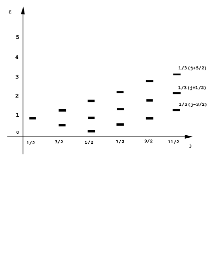
Figure 2: The positive part of spectrum of the $\Gamma_{0}$ matrix for N=3. One can clearly see the appearance of eigenvalues which are less than unity, $\epsilon<1$.

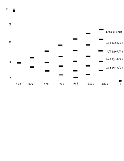
Figure 3: The positive part of spectrum of the $\Gamma_{0}$ matrix for N=5. The number of states with $\epsilon<1$ increases. As N tends to infinity the spectral cone $j=[1/2,N-1/2]$ becomes more ”narrow” and the eigenvalues are concentrated around $\epsilon=1$.

5.4 N pairs of adjoint representations

In this case we shall take $\Theta=(\Theta_{\dot{N}},\cdots,\Theta_{\dot{1}},\Theta_{1},\cdots,\Theta_{N})$ which can be rewritten also in the form (19)

$$(N-1/2;-\lambda),~{}~{}~{}\cdots~{}~{}~{},(1/2;-\lambda)~{},~{}(1/2;\lambda),~{}~{}~{}\cdots~{}~{}~{},(N-1/2;\lambda),$$ (85)

the wave function has the form

$$\Psi=\left(\begin{array}[]{c}\Psi^{r}_{jm}\\ \Psi^{\dot{r}}_{jm}\end{array}\right)~{}~{}~{}~{}~{}~{}~{}~{}r=1,...,N;~{}~{}~{}~{}~{}~{}j=r-1/2,~{}r+1/2,...;~{}~{}~{}~{}~{}~{}~{}m=-j,...,j$$

Then the transition amplitudes are equal to

$$\lambda^{r}_{j}=-\lambda^{\dot{r}}_{j}=i~{}\frac{r-1/2}{j(j+1)}~{}\lambda~{}~{}~{}~{}~{}~{}~{}~{}~{}~{}~{}~{}~{}~{}~{}j\geq r-1/2$$

and

$$\varsigma^{r}_{j}=\varsigma^{\dot{r}}_{j}=\frac{1}{2}\sqrt{(1-\frac{r^{2}-r}{j^{2}-1/4})(1-(\frac{\lambda}{j})^{2})}~{}~{}~{}~{}~{}~{}j\geq r+1/2$$

where $~{}~{}~{}r=1,...,N$.

Our basic solution ( B-solution) of the equation (57) for the $\Gamma_{0}$ in this general case is a $~{}2N\times 2N~{}$ Jacoby matrix with the following nonzero elements

$$\gamma^{r+1~{}r}_{j}=\gamma^{r~{}r+1}_{j}=\gamma^{\dot{r+1}~{}\dot{r}}_{j}=\gamma^{\dot{r}~{}\dot{r+1}}_{j}=i~{}\sqrt{(1-\frac{r^{2}}{N^{2}})~{}(\frac{j^{2}+j}{4r^{2}-1}-\frac{1}{4})}~{}~{}~{}~{}~{}j\geq r+1/2$$ (86)

$$\gamma^{1~{}\dot{1}}_{j}=\gamma^{\dot{1}~{}1}_{j}=j+1/2$$ (87)

here $r=1,...,N-1$. The gamma matrices for the first few values of $j$ are equal to

$$\gamma_{1/2}=\left(\begin{array}[]{c}0,~{}~{}~{}~{}~{}~{}1\\ 1,~{}~{}~{}~{}~{}~{}0\end{array}\right),~{}~{}\gamma_{3/2}=\left(\begin{array}[]{c}0,~{}~{}~{}~{}~{}~{}~{}~{}~{}~{}~{}~{}~{}i\sqrt{1-1/N^{2}},{}{}{}{}{}{}{}{}{}{}{}{}{}{}{}{}{}{}{}{}{}{}{}\\ i\sqrt{1-1/N^{2}},~{}~{}~{}~{}~{}0,~{}~{}~{}~{}~{}~{}2,{}{}{}{}{}{}{}{}{}{}{}{}{}{}{}{}{}{}{}{}{}{}{}\\ ~{}~{}~{}~{}~{}~{}~{}~{}~{}~{}~{}~{}~{}~{}~{}~{}~{}~{}~{}~{}~{}~{}~{}~{}2,~{}~{}~{}~{}~{}~{}0,~{}~{}~{}~{}~{}~{}~{}~{}~{}~{}i\sqrt{1-1/N^{2}}\\ ~{}~{}~{}~{}~{}~{}~{}~{}~{}~{}~{}~{}~{}~{}~{}~{}~{}~{}~{}~{}~{}~{}~{}~{}~{}~{}~{}~{}i\sqrt{1-1/N^{2}},~{}~{}~{}~{}~{}~{}~{}~{}~{}~{}~{}0\end{array}\right),$$

$$\gamma_{5/2}=\left(\begin{array}[]{c}0,~{}~{}~{}~{}~{}~{}i\sqrt{(1-4/N^{2})(1/3)},{}{}{}{}{}{}{}{}{}{}{}{}{}{}{}{}{}{}{}{}{}{}\\ i\sqrt{(1-4/N^{2})(1/3)},~{}~{}~{}~{}~{}0,~{}~{}~{}~{}~{}~{}~{}~{}~{}~{}i\sqrt{(1-1/N^{2})(8/3)},{}{}{}{}{}{}{}{}{}{}{}{}{}{}{}{}{}\\ ~{}~{}~{}~{}~{}~{}~{}~{}~{}~{}~{}~{}~{}i\sqrt{(1-1/N^{2})(8/3)},~{}~{}~{}~{}0,~{}~{}~{}~{}~{}~{}~{}~{}~{}~{}3,{}{}{}{}{}{}{}\\ ~{}~{}~{}~{}~{}~{}~{}~{}~{}~{}~{}~{}~{}~{}~{}~{}~{}~{}~{}~{}~{}~{}~{}~{}~{}~{}~{}~{}~{}~{}~{}~{}~{}~{}~{}~{}~{}~{}~{}~{}~{}3,~{}~{}~{}~{}~{}~{}~{}~{}~{}~{}0,~{}~{}~{}~{}~{}i\sqrt{(1-1/N^{2})(8/3)},{}{}{}{}{}{}{}{}{}\\ ~{}~{}~{}~{}~{}~{}~{}~{}~{}~{}~{}~{}~{}~{}~{}~{}~{}~{}~{}~{}~{}~{}~{}~{}~{}~{}i\sqrt{(1-1/N^{2})(8/3)},~{}~{}~{}0,~{}~{}~{}i\sqrt{(1-4/N^{2})(1/3)}\\ ~{}~{}~{}~{}~{}~{}~{}~{}~{}~{}~{}~{}~{}~{}~{}~{}~{}~{}~{}~{}~{}~{}~{}~{}~{}~{}~{}~{}~{}~{}~{}~{}~{}~{}~{}~{}~{}~{}~{}i\sqrt{(1-4/N^{2})(1/3)},~{}~{}~{}0\end{array}\right),$$

and they grow in size with $j$ until $j=N-1/2$, for greater $j$ the size of the matrix $\gamma_{j}$ remains the same and is equal to $2N\times 2N$. The determinant of the $\gamma_{j}$ matrix for $j$ in the interval $[3/2,~{}7/2,...,N-1/2]$ is equal to

$$Det~{}\gamma_{j}=(1-1/N^{2})^{2}~{}\cdots~{}(1-(j-1/2)^{2}/N^{2})^{2}$$ (88)

and for $j$ in the interval $[1/2,~{}5/2,...,N-1/2]$ is

$$Det~{}\gamma_{j}=(-1)(1-4/N^{2})^{2}~{}\cdots~{}(1-(j-1/2)^{2}/N^{2})^{2}.$$ (89)

From the determinant and the trace of the gamma matrix it follows that

$$\epsilon_{1}^{2}\cdot...\cdot\epsilon_{j+1/2}^{2}=|Det~{}\gamma_{j}|~{}~{}~{}~{}~{}~{}~{}~{}\epsilon_{1}^{2}+...+\epsilon_{j+1/2}^{2}=\frac{1}{2}Tr~{}\gamma^{2}_{j}~{}~{}~{}~{}j\geq(N-1/2).$$ (90)

The characteristic equations for these matrices are:

$$\gamma^{2}_{1/2}-1=0,$$

$$((\gamma_{3/2}-1)^{2}-1/N^{2})~{}((\gamma_{3/2}+1)^{2}-1/N^{2})=0,$$

$$(\gamma^{2}_{5/2}-1)~{}((\gamma_{5/2}-1)^{2}-4/N^{2})~{}((\gamma_{5/2}+1)^{2}-4/N^{2})=0,$$

$$.~{}.~{}.~{}.~{}.~{}.~{}.~{}.~{}.~{}.~{}.~{}.~{}.~{}.~{}.~{}.~{}.~{}.~{}.~{}.~{}.~{}.~{}.~{}.~{}.~{}.~{}.~{}.~{}.~{}.~{}.~{}.~{}.~{}.~{}.~{}.~{}.~{}.~{}.~{}.~{}.~{}.$$

$$\cdots(\gamma^{2}_{j}-(1+(j-5/2)/N)^{2})~{}(\gamma^{2}_{j}-(1+(j-1/2)/N)^{2})=0,$$ (91)

where in the last equation $j\geq N-1/2$. The positive eigenvalues $\epsilon_{j}$ can be now found

$$1~{}~{}~{}~{}~{}~{}~{}~{}~{}~{}~{}~{}~{}~{}~{}~{}~{}~{}~{}~{}~{}~{}~{}~{}~{}~{}~{}~{}~{}j=1/2$$

$$1-1/N~{}~{}~{}~{}~{}~{}~{}~{}1+1/N~{}~{}~{}~{}~{}~{}~{}~{}~{}~{}~{}~{}~{}~{}~{}~{}~{}~{}~{}~{}~{}~{}~{}~{}~{}~{}~{}~{}~{}~{}~{}~{}j=3/2$$

$$1-2/N~{}~{}~{}~{}1~{}~{}~{}1+2/N~{}~{}~{}~{}~{}~{}~{}~{}~{}~{}~{}~{}~{}~{}~{}~{}~{}~{}~{}~{}~{}~{}~{}~{}~{}~{}~{}~{}~{}~{}~{}~{}j=5/2$$

$$1-3/N~{}~{}~{}~{}1-1/N~{}~{}~{}~{}~{}1+1/N~{}~{}~{}~{}1+3/N~{}~{}~{}~{}~{}~{}~{}~{}~{}~{}~{}~{}~{}~{}~{}~{}~{}~{}~{}~{}~{}~{}~{}~{}~{}j=7/2$$

$$1-4/N~{}~{}~{}~{}1-2/N~{}~{}1~{}~{}1+2/N~{}~{}~{}~{}1+4/N~{}~{}~{}~{}~{}~{}~{}~{}~{}~{}~{}~{}~{}~{}~{}~{}~{}~{}~{}~{}~{}~{}~{}~{}~{}j=9/2$$

. . . . . . . . . . . . . . . . . . . . . . . . . . . . . . .  . . . . .

$$\cdots~{}~{},1+(j-5/2)/N,~{}~{}~{}1+(j-1/2)/N~{}~{}~{}~{}~{}~{}~{}~{}~{}j\geq N-1/2$$ (92)

On Fig.2,3 one can see the spectrum of the matrix $\gamma_{j}$ as a functin of $j$.

The number of states with angular momentum $j$ grows as $j+1/2$ and this takes place up to spin $j=N-1/2$. For the higher spins $j\geq N-1/2$ the number of states remains constant and is equal to $N$ (see Fig.2,3). Thus we see that the coefficient of proportionality drops N times and many eigenvalues are less than unity. The mass spectrum is bounded from bellow only if all eigenvalues are less than unity.

6 Nonhermitian Solution of $\Gamma_{0}$. $N\rightarrow\infty$.

In the limit $N\rightarrow\infty$ our solution (86) is being reduced to the form

$$\gamma^{r+1~{}r}_{j}=\gamma^{r~{}r+1}_{j}=\gamma^{\dot{r+1}~{}\dot{r}}_{j}=\gamma^{\dot{r}~{}\dot{r+1}}_{j}=i~{}\sqrt{(\frac{j^{2}+j}{4r^{2}-1}-\frac{1}{4})}~{}~{}~{}~{}~{}j\geq r+1/2$$ (93)

$$\gamma^{1~{}\dot{1}}_{j}=\gamma^{\dot{1}~{}1}_{j}=j+1/2$$ (94)

where $r=1,2,...$. As it is easy to see from the previous formulas, all eigenvalues $\epsilon_{j}$ tend to unity when number of representations $N\rightarrow\infty$. The characteristic equation which is satisfied by the gamma matrix in this limit is

$$(\gamma_{j}^{2}-1)^{j+1/2}=0~{}~{}~{}~{}~{}~{}~{}~{}~{}~{}j=1/2,~{}3/2,~{},5/2,\cdots$$ (95)

with all eigenvalues $\epsilon_{j}=\pm 1$ (see Fig.4).

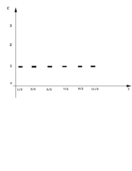
Figure 4: The positive part of the spectrum of the $\Gamma_{0}$ matrix for $N=\infty$.

The determinant and the trace are equal to

$$Det~{}\gamma_{j}=\pm 1~{}~{}~{}~{}~{}Tr~{}\gamma^{2}_{j}=2j+1,$$ (96)

thus

$$\epsilon_{1}^{2}\cdot...\cdot\epsilon_{j+1/2}^{2}=1~{}~{}~{}~{}~{}~{}\epsilon_{1}^{2}+...+\epsilon_{j+1/2}^{2}=j+1/2$$ (97)

The matrix $\Omega~{}\Gamma_{0}$ has the characteristic equation

$$(\omega_{j}~{}\gamma_{j}-1)^{2j+1}=0$$ (98)

with all eigenvalues equal to $\rho_{j}=+1$, therefore introducing

$$\omega_{j}~{}\gamma_{j}-1=\sigma_{j}$$ (99)

we have an important relation

$$\sigma^{2j+1}_{j}=0$$ (100)

and

$$\gamma_{j}=\omega_{j}(~{}1+~{}\sigma_{j}~{})$$ (101)

The $\sigma_{j}$ defines the algebra of elements

$$\sigma_{j},~{}\sigma^{+}_{j},~{}\sigma^{2}_{j},~{}\sigma^{+~{}2}_{j},...,\sigma^{2j}_{j},~{}\sigma^{+~{}2j}_{j}$$ (102)

with the property

$$\sigma^{2j+1}_{j}=\sigma^{+~{}2j+1}_{j}=0$$ (103)

Thus the matrix $\Omega~{}\Gamma_{0}$ is positive definite and all its eigenvalues are equal to one, but the important relations

$$\Omega~{}\Gamma_{0}\neq\Gamma^{+}_{0}~{}\Omega~{}~{}~{}~{}~{}~{}\Gamma^{+}_{0}\neq\Gamma_{0}$$ (104)

are not held and therefore the Hamiltonian is not Hermitian. In the next section we shall find the Hermitian solution for $\Gamma_{0}$ using the fact that one can change the phases of the matrix elements without disturbing its determinant.

7 Hermitian solution for $\Gamma_{0}$

The Hermitian solution (H-solution) of (57) for $\Gamma_{0}$ can be found as a phase modification of our basic B-solution (86)

$$\gamma^{r+1~{}r}_{j}=-\gamma^{r~{}r+1}_{j}=-\gamma^{\dot{r+1}~{}\dot{r}}_{j}=\gamma^{\dot{r}~{}\dot{r+1}}_{j}=i~{}\sqrt{(\frac{j^{2}+j}{4r^{2}-1}-\frac{1}{4})}~{}~{}~{}~{}~{}j\geq r+1/2$$ (105)

$$\gamma^{1~{}\dot{1}}_{j}=\gamma^{\dot{1}~{}1}_{j}=j+1/2$$ (106)

which for low values of $j$ is:

$$\gamma_{1/2}=\left(\begin{array}[]{c}0,~{}~{}~{}1\\ 1,~{}~{}~{}0\end{array}\right),~{}~{}\gamma_{3/2}=\left(\begin{array}[]{c}0,~{}~{}~{}i,{}{}{}{}{}{}{}{}{}\\ -i,~{}~{}0,~{}~{}~{}2,{}{}{}{}\\ ~{}~{}~{}~{}~{}2,~{}~{}~{}0,~{}~{}~{}i\\ ~{}~{}~{}~{}~{}~{}~{}~{}~{}-i,~{}~{}~{}0\end{array}\right),$$

$$\gamma_{5/2}=\left(\begin{array}[]{c}~{}~{}~{}~{}~{}0,~{}~{}~{}~{}~{}i\sqrt{1/3},{}{}{}{}{}{}{}{}{}{}{}{}{}{}{}{}{}{}{}{}{}{}{}{}{}{}{}{}{}{}{}{}{}{}{}{}{}{}\\ -i\sqrt{1/3},~{}~{}~{}0,~{}~{}~{}i\sqrt{8/3},{}{}{}{}{}{}{}{}{}{}{}{}{}{}{}{}{}{}{}{}{}{}{}{}{}{}{}{}{}\\ ~{}~{}~{}~{}~{}~{}~{}~{}~{}~{}~{}-i\sqrt{8/3},~{}~{}~{}0,~{}~{}~{}~{}3,{}{}{}{}{}{}{}{}{}{}{}{}{}{}{}{}{}{}{}{}{}{}{}{}{}{}{}\\ ~{}~{}~{}~{}~{}~{}~{}~{}~{}~{}~{}~{}~{}~{}~{}~{}~{}~{}~{}~{}~{}~{}~{}~{}~{}~{}~{}3,~{}~{}~{}~{}0,~{}~{}~{}~{}i\sqrt{8/3},{}{}{}{}{}{}{}{}{}{}{}\\ ~{}~{}~{}~{}~{}~{}~{}~{}~{}~{}~{}~{}~{}~{}~{}~{}~{}~{}~{}~{}~{}~{}~{}~{}~{}~{}~{}~{}-i\sqrt{8/3},~{}~{}~{}0,~{}~{}~{}~{}~{}i\sqrt{1/3}\\ ~{}~{}~{}~{}~{}~{}~{}~{}~{}~{}~{}~{}~{}~{}~{}~{}~{}~{}~{}~{}~{}~{}~{}~{}~{}~{}~{}~{}~{}~{}~{}~{}~{}~{}~{}~{}~{}~{}~{}-i\sqrt{1/3},~{}~{}~{}~{}0{}{}{}{}{}\end{array}\right),...$$

These matrices are Hermitian $\Gamma^{+}_{0}=\Gamma_{0}$, but the characteristic equations are more complicated now:

$$\gamma^{2}_{1/2}-1=0,$$

$$(\gamma^{2}_{3/2}-2\gamma_{3/2}-1)~{}(\gamma^{2}_{3/2}+2\gamma_{3/2}-1)=0,$$

$$(\gamma^{2}_{5/2}-1)~{}(\gamma^{2}_{5/2}-4\gamma_{5/2}+1)~{}(\gamma^{2}_{5/2}+4\gamma_{5/2}+1)=0,$$

$$(\gamma^{4}_{7/2}+4\gamma^{3}_{7/2}-6\gamma^{2}_{7/2}-4\gamma_{7/2}+1)(\gamma^{4}_{7/2}-4\gamma^{3}_{7/2}-6\gamma^{2}_{7/2}+4\gamma_{7/2}+1)=0,$$

$$(\gamma^{2}_{9/2}-1)~{}(\gamma^{4}_{9/2}+4\gamma^{3}_{9/2}-14\gamma^{2}_{9/2}+4\gamma_{9/2}+1)~{}(\gamma^{4}_{9/2}-4\gamma^{3}_{9/2}-14\gamma^{2}_{9/2}-4\gamma_{9/2}+1)=0,$$

$$.~{}.~{}.~{}.~{}.~{}.~{}.~{}.~{}.~{}.~{}.~{}.~{}.~{}.~{}.~{}.~{}.~{}.~{}.~{}.~{}.~{}.~{}.~{}.~{}.~{}.~{}.~{}.~{}.~{}.~{}.~{}.~{}.~{}.~{}.~{}.~{}.~{}.~{}.~{}.~{}.~{}.~{}.~{}.~{}.~{}.~{}.~{}.~{}.~{}.~{}.~{}.~{}.~{}.~{}.~{}.~{}.~{}.~{}.$$

These polynomials $p(\epsilon)$ have the reflective symmetry and are even

$$p_{j}(\epsilon)~{}=~{}\epsilon^{2j+1}~{}p_{j}(1/\epsilon)$$ (108)

$$p_{j}(-\epsilon)~{}=~{}p_{j}(\epsilon)$$ (109)

therefore if $\epsilon_{j}$ is a solution then $1/\epsilon_{j}$,$-\epsilon_{j}$ and $-1/\epsilon_{j}$ are also solutions. Computing the traces and determinants of these matrices one can get the following general relation for the eigenvalues

$$\epsilon_{1}^{2}\cdot...\cdot\epsilon_{j+1/2}^{2}=1~{}~{}~{}~{}~{}~{}~{}~{}\epsilon_{1}^{2}+...+\epsilon_{j+1/2}^{2}=j(2j+1).$$ (110)

The eigenvalues $\epsilon_{j}$ can be now found

$$~{}~{}~{}~{}~{}~{}~{}~{}~{}~{}~{}~{}~{}~{}~{}~{}~{}~{}~{}1~{}~{}~{}~{}~{}~{}~{}~{}~{}~{}~{}~{}~{}~{}~{}~{}~{}~{}~{}~{}~{}~{}~{}~{}~{}~{}~{}~{}~{}~{}~{}~{}~{}~{}~{}j=1/2$$

$$~{}~{}~{}~{}~{}~{}~{}~{}~{}~{}~{}~{}~{}~{}~{}~{}~{}\sqrt{2}-1~{}~{}~{}~{}~{}~{}~{}~{}\sqrt{2}+1~{}~{}~{}~{}~{}~{}~{}~{}~{}~{}~{}~{}~{}~{}~{}~{}~{}~{}~{}~{}~{}~{}~{}~{}~{}~{}~{}~{}~{}~{}~{}~{}~{}~{}j=3/2$$

$$~{}~{}~{}~{}~{}~{}~{}~{}~{}~{}~{}~{}~{}~{}~{}~{}~{}2-\sqrt{3}~{}~{}~{}~{}1~{}~{}~{}~{}2+\sqrt{3}~{}~{}~{}~{}~{}~{}~{}~{}~{}~{}~{}~{}~{}~{}~{}~{}~{}~{}~{}~{}~{}~{}~{}~{}~{}~{}~{}~{}~{}~{}~{}~{}~{}~{}j=5/2$$

$$\sqrt{(\sqrt{2}+1)^{2}+1}-(\sqrt{2}+1)~{}~{}~{}~{}~{}~{}~{}~{}\sqrt{(\sqrt{2}-1)^{2}+1}-(\sqrt{2}-1)~{}~{}~{}~{}~{}~{}~{}~{}~{}~{}~{}~{}~{}j=7/2$$

$$\sqrt{(\sqrt{2}-1)^{2}+1}+(\sqrt{2}-1)~{}~{}~{}~{}~{}~{}~{}~{}\sqrt{(\sqrt{2}+1)^{2}+1}+(\sqrt{2}+1)~{}~{}~{}~{}~{}~{}~{}~{}~{}~{}~{}~{}~{}j=7/2$$

$$\sqrt{5}+1-\sqrt{(\sqrt{5}+1)^{2}-1}~{}~{}~{}~{}~{}~{}~{}~{}\sqrt{5}-1-\sqrt{(\sqrt{5}-1)^{2}-1}~{}~{}~{}~{}~{}~{}~{}~{}~{}~{}~{}~{}~{}j=9/2$$

$$~{}~{}~{}~{}~{}~{}~{}~{}~{}~{}~{}~{}~{}~{}~{}~{}~{}~{}~{}~{}~{}~{}~{}~{}~{}~{}~{}~{}~{}~{}~{}~{}~{}1~{}~{}~{}~{}~{}~{}~{}~{}~{}~{}~{}~{}~{}~{}~{}~{}~{}~{}~{}~{}~{}~{}~{}~{}~{}~{}~{}~{}~{}~{}~{}~{}~{}~{}~{}~{}~{}~{}~{}~{}~{}~{}~{}~{}~{}~{}~{}~{}~{}j=9/2$$

$$\sqrt{5}-1+\sqrt{(\sqrt{5}-1)^{2}-1}~{}~{}~{}~{}~{}~{}~{}~{}\sqrt{5}+1+\sqrt{(\sqrt{5}+1)^{2}-1}~{}~{}~{}~{}~{}~{}~{}~{}~{}~{}~{}~{}~{}j=9/2$$

$$.~{}.~{}.~{}.~{}.~{}.~{}.~{}.~{}.~{}.~{}.~{}.~{}.~{}.~{}.~{}.~{}.~{}.~{}.~{}.~{}.~{}.~{}.~{}.~{}.~{}.~{}.~{}.~{}.~{}.~{}.~{}.~{}.~{}.~{}.~{}.$$ (111)

The changes of the phases in the matrix elements (105) result into different behaviour of eigenvalues (see Fig.5).

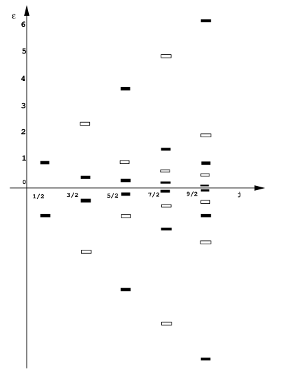
Figure 5: The spectrum of the $\Gamma_{0}$ matrix for the Hermitian solution (H-solution). The quasilinear trajectories have different slope. One can observe also approximate hyperbolic curves on which lie the eigenvalues from different trajectories. The symmetric solution ($\Sigma$-solution) has the same spectrum.

The matrix $\Omega~{}\Gamma_{0}$ has again the characteristic equation

$$(\omega_{j}~{}\gamma_{j}-1)^{2j+1}=0$$ (112)

and all eigenvalues are equal to one. Thus again the matrix $\Omega~{}\Gamma_{0}$ is positive definite because all eigenvalues are equal to one, but the important relation

$$\Omega~{}\Gamma_{0}\neq\Gamma^{+}_{0}~{}\Omega$$ (113)

does not hold. Introducing

$$\omega_{j}~{}\gamma_{j}-1=~{}\tau_{j}$$ (114)

we have the relation

$$\tau_{j}^{2j+1}=0$$ (115)

and

$$\gamma_{j}=\omega_{j}(~{}1+~{}\tau_{j})$$ (116)

The $\tau_{j}$ defines the algebra of elements

$$\tau_{j},~{}\tau^{+}_{j},~{}\tau^{2}_{j},~{}\tau^{+~{}2}_{j},...,\tau^{2j}_{j},~{}\tau^{+~{}2j}_{j}$$ (117)

with the property

$$\tau^{2j+1}_{j}=\tau^{+~{}2j+1}_{j}=0.$$ (118)

8 Real and symmetric solution for $\Gamma_{0}$

The solution of (57) for $\Gamma_{0}$ with necessary properties can be found by using our basic solutions (86) rewritten with arbitrary phases of the matrix elements and then by requiring that $\Gamma_{0}$ should be Hermitian $\Gamma^{+}_{0}=\Gamma_{0}$ and should satisfy the relations $\Gamma^{+}_{0}~{}\Omega=\Omega~{}\Gamma_{0}$. The symmetric $\Sigma$-solution is

$$\gamma^{r+1~{}r}_{j}=~{}\gamma^{r~{}r+1}_{j}=\gamma^{\dot{r+1}~{}\dot{r}}_{j}=\gamma^{\dot{r}~{}\dot{r+1}}_{j}=\sqrt{(\frac{j^{2}+j}{4r^{2}-1}-\frac{1}{4})}~{}~{}~{}~{}~{}j\geq r+1/2$$ (119)

$$\gamma^{1~{}\dot{1}}_{j}=\gamma^{\dot{1}~{}1}_{j}=j+1/2$$ (120)

which for the low values of $j$ is:

$$\gamma_{1/2}=\left(\begin{array}[]{c}0,~{}~{}~{}1\\ 1,~{}~{}~{}0\end{array}\right),~{}~{}\gamma_{3/2}=\left(\begin{array}[]{c}0,~{}~{}~{}1,{}{}{}{}{}{}{}{}{}\\ 1,~{}~{}0,~{}~{}~{}2,{}{}{}{}\\ ~{}~{}~{}~{}~{}2,~{}~{}~{}0,~{}~{}~{}1\\ ~{}~{}~{}~{}~{}~{}~{}~{}~{}1,~{}~{}~{}0\end{array}\right),$$ (121)

$$\gamma_{5/2}=\left(\begin{array}[]{c}~{}~{}~{}~{}~{}0,~{}~{}~{}~{}~{}\sqrt{1/3},{}{}{}{}{}{}{}{}{}{}{}{}{}{}{}{}{}{}{}{}{}{}{}{}{}{}{}{}{}{}{}{}{}{}{}{}{}{}\\ \sqrt{1/3},~{}~{}~{}0,~{}~{}~{}\sqrt{8/3},{}{}{}{}{}{}{}{}{}{}{}{}{}{}{}{}{}{}{}{}{}{}{}{}{}{}{}{}{}\\ ~{}~{}~{}~{}~{}~{}~{}~{}~{}~{}~{}\sqrt{8/3},~{}~{}~{}0,~{}~{}~{}~{}3,{}{}{}{}{}{}{}{}{}{}{}{}{}{}{}{}{}{}{}{}{}{}{}{}{}{}{}\\ ~{}~{}~{}~{}~{}~{}~{}~{}~{}~{}~{}~{}~{}~{}~{}~{}~{}~{}~{}~{}~{}~{}~{}~{}~{}~{}~{}3,~{}~{}~{}~{}0,~{}~{}~{}~{}\sqrt{8/3},{}{}{}{}{}{}{}{}{}{}{}\\ ~{}~{}~{}~{}~{}~{}~{}~{}~{}~{}~{}~{}~{}~{}~{}~{}~{}~{}~{}~{}~{}~{}~{}~{}~{}~{}~{}~{}\sqrt{8/3},~{}~{}~{}0,~{}~{}~{}~{}~{}\sqrt{1/3}\\ ~{}~{}~{}~{}~{}~{}~{}~{}~{}~{}~{}~{}~{}~{}~{}~{}~{}~{}~{}~{}~{}~{}~{}~{}~{}~{}~{}~{}~{}~{}~{}~{}~{}~{}~{}~{}~{}~{}~{}\sqrt{1/3},~{}~{}~{}~{}0{}{}{}{}{}\end{array}\right),...$$

In this case we have Hermitian matrix $\Gamma^{+}_{0}=\Gamma_{0}$ which has the desired property

$$\Gamma^{+}_{0}~{}\Omega=\Omega~{}\Gamma_{0}.$$ (122)

This means that the charge density is equal to $\rho=\Omega~{}\Gamma_{0}$. In addition all gamma matrices now have this property (45)

$$\Gamma^{+}_{k}~{}\Omega=\Omega~{}\Gamma_{k}~{}~{}~{}~{}~{}k=x,y,z$$ (123)

which follows from the definition of $\Gamma_{k}=i[b_{k}~{}\Gamma_{0}]$ and equation (33) $\Omega~{}b_{k}~{}=b^{+}_{k}~{}\Omega$.

The characteristic equations for the first few values of $j$ are

$$\gamma^{2}_{1/2}-1=0,$$

$$(\gamma^{2}_{3/2}-2\gamma_{3/2}-1)~{}(\gamma^{2}_{3/2}+2\gamma_{3/2}-1)=0,$$

$$(\gamma^{2}_{5/2}-1)~{}(\gamma^{2}_{5/2}-4\gamma_{5/2}+1)~{}(\gamma^{2}_{5/2}+4\gamma_{5/2}+1)=0,$$

$$(\gamma^{2}_{7/2}+2(\sqrt{2}-1)\gamma_{7/2}-1)~{}(\gamma^{2}_{7/2}-2(\sqrt{2}+1)\gamma_{7/2}-1)~{}~{}~{}~{}~{}~{}~{}$$

$$(\gamma^{2}_{7/2}+2(\sqrt{2}+1)\gamma_{7/2}-1)~{}(\gamma^{2}_{7/2}-2(\sqrt{2}-1)\gamma_{7/2}-1)=0,$$

$$(\gamma^{2}_{9/2}-1)~{}(\gamma^{2}_{9/2}+2(\sqrt{5}-1)\gamma_{9/2}+1)~{}(\gamma^{2}_{9/2}-2(\sqrt{5}+1)\gamma_{9/2}+1)~{}~{}~{}~{}~{}~{}~{}$$

$$(\gamma^{2}_{9/2}+2(\sqrt{5}+1)\gamma_{9/2}+1)~{}(\gamma^{2}_{9/2}-2(\sqrt{5}-1)\gamma_{9/2}+1)=0,$$

$$.~{}.~{}.~{}.~{}.~{}.~{}.~{}.~{}.~{}.~{}.~{}.~{}.~{}.~{}.~{}.~{}.~{}.~{}.~{}.~{}.~{}.~{}.~{}.~{}.~{}.~{}.~{}.~{}.~{}.~{}.~{}.~{}.~{}.~{}.~{}.~{}.~{}.~{}.~{}.~{}.~{}.~{}.~{}.~{}$$ (124)

and the spectrum (111) (see Fig.5) is the same for the Hermitian H-solution and symmetric $\Sigma$-solution. The corresponding characteristic equations for the matrices $\rho_{j}$ are

$$(\rho_{1/2}-1)^{2}=0,$$

$$(\rho^{2}_{3/2}-2\rho_{3/2}-1)^{2}=0,$$

$$(\rho_{5/2}+1)^{2}~{}(\rho^{2}_{5/2}-4\rho_{5/2}+1)^{2}=0,$$

$$(\rho^{4}_{7/2}-4\rho^{3}_{7/2}-6\rho^{2}_{7/2}+4\rho_{7/2}+1)^{2}=0,$$

$$(\rho_{9/2}-1)^{2}(\rho^{4}_{9/2}-4\rho^{3}_{9/2}-14\rho^{2}_{9/2}-4\rho_{9/2}+1)^{2}=0,$$

$$.~{}.~{}.~{}.~{}.~{}.~{}.~{}.~{}.~{}.~{}.~{}.~{}.~{}.~{}.~{}.~{}.~{}.~{}.~{}.~{}.~{}.~{}.~{}.~{}.~{}.~{}.~{}.~{}.~{}.~{}.~{}.~{}.~{}.~{}.~{}.~{}.~{}.$$

and the eigenvalues of the density matrix are equal therefore to

$$~{}~{}~{}~{}~{}~{}~{}~{}~{}~{}~{}~{}~{}~{}~{}~{}~{}~{}~{}~{}~{}~{}~{}~{}~{}1~{}~{}~{}~{}~{}~{}~{}~{}~{}~{}1~{}~{}~{}~{}~{}~{}~{}~{}~{}~{}~{}~{}~{}~{}~{}~{}~{}~{}~{}~{}~{}~{}~{}~{}~{}~{}~{}~{}~{}~{}~{}~{}~{}~{}~{}~{}~{}j=1/2$$

$$~{}~{}~{}~{}~{}~{}~{}~{}~{}~{}~{}~{}~{}~{}~{}~{}~{}1-\sqrt{2}~{}~{}~{}~{}~{}~{}~{}~{}\sqrt{2}+1~{}~{}~{}~{}~{}~{}~{}~{}~{}~{}~{}~{}~{}~{}~{}~{}~{}~{}~{}~{}~{}~{}~{}~{}~{}~{}~{}~{}~{}~{}~{}~{}j=3/2$$

$$~{}~{}~{}~{}~{}~{}~{}~{}~{}~{}~{}~{}~{}~{}~{}~{}~{}2-\sqrt{3}~{}~{}~{}~{}-1~{}~{}~{}~{}2+\sqrt{3}~{}~{}~{}~{}~{}~{}~{}~{}~{}~{}~{}~{}~{}~{}~{}~{}~{}~{}~{}~{}~{}~{}~{}~{}~{}~{}~{}~{}~{}~{}~{}~{}j=5/2$$

$$(1+\sqrt{2})+\sqrt{(\sqrt{2}+1)^{2}+1}~{}~{}~{}~{}~{}~{}(1+\sqrt{2})-\sqrt{(\sqrt{2}+1)^{2}+1}~{}~{}~{}~{}~{}~{}~{}~{}~{}~{}~{}j=7/2$$

$$(1-\sqrt{2})+\sqrt{(\sqrt{2}-1)^{2}+1}~{}~{}~{}~{}~{}(1-\sqrt{2})-\sqrt{(\sqrt{2}-1)^{2}+1}~{}~{}~{}~{}~{}~{}~{}~{}~{}~{}~{}j=7/2$$

$$1+\sqrt{5}+\sqrt{(\sqrt{5}+1)^{2}-1}~{}~{}~{}~{}~{}~{}~{}~{}1+\sqrt{5}-\sqrt{(\sqrt{5}+1)^{2}-1}~{}~{}~{}~{}~{}~{}~{}~{}~{}~{}~{}~{}j=9/2$$

$$~{}~{}~{}~{}~{}~{}~{}~{}~{}~{}~{}~{}~{}~{}~{}~{}~{}~{}~{}~{}~{}~{}~{}~{}~{}~{}~{}~{}~{}~{}~{}~{}~{}~{}~{}~{}1~{}~{}~{}~{}~{}~{}~{}~{}~{}~{}~{}~{}~{}~{}~{}~{}~{}~{}~{}~{}~{}~{}~{}~{}~{}~{}~{}~{}~{}~{}~{}~{}~{}~{}~{}~{}~{}~{}~{}~{}~{}~{}~{}~{}~{}~{}~{}~{}~{}j=9/2$$

$$1-\sqrt{5}+\sqrt{(\sqrt{5}-1)^{2}-1}~{}~{}~{}~{}~{}~{}~{}~{}1-\sqrt{5}-\sqrt{(\sqrt{5}-1)^{2}-1}~{}~{}~{}~{}~{}~{}~{}~{}~{}~{}~{}~{}j=9/2$$

$$.~{}.~{}.~{}.~{}.~{}.~{}.~{}.~{}.~{}.~{}.~{}.~{}.~{}.~{}.~{}.~{}.~{}.~{}.~{}.~{}.~{}.~{}.~{}.~{}.~{}.~{}.~{}.~{}.~{}.~{}.~{}.~{}.~{}.~{}.~{}.~{}.~{}.~{}.~{}.~{}.~{}.~{}.~{}.~{}.$$ (126)

Both states with $j=1/2$ have positive norms, the $j=3/2$ level has two positive and two negative norm states, the $j=5/2$ has four positive and two negative norm states, the $j=7/2$ has four positive and four negative norm states, the $j=9/2$ have six positive and four negative norm states, and so on (see Fig.5). On the Figure 6 one can see the mass spectrum of the $\Sigma$-equation. The positive norm physical states, marked by the black bricks, are lying on the quasilinear trajectories and the negative norm ghost states, marked by the white bricks, are also lying on the quasilinear trajectories of different slope. Thus we have the equation which has the increasing mass spectrum, but the smallest mass on a given trajectory still tends to zero and in addition we have infinitely many ghost states. In the next section we shall solve the problem of decreasing behaviour of the smallest mass on a given trajectory, but before that let us remark that one can project out the unwanted ghost states by constructing the projection operator

$$Pr=\prod_{i}(1+\frac{1}{\epsilon_{i}}\Omega\Gamma_{0})$$ (127)

where the product is over ghost states. The details will be given in the second part of this work where we shall formulate natural constraints which appear in this system.

Figure 6: The mass spectrum of $H=M\Gamma^{-1}_{0}$. One can see positive norm physical states, marked by the black bricks, lying on the quasilinear trajectories and negative norm ghost states, marked by the white bricks, also lying on the quasilinear trajectories of different slope.

8.1 Equation for the spin j components of the wave function

Let us consider only a time dependent $\Sigma$-equation

$$i~{}\Gamma_{0}~{}\dot{\Psi}~{}=~{}M~{}\Psi~{}~{}~{}~{}~{}~{}~{}i~{}\dot{\Psi}~{}=\Gamma^{-1}_{0}~{}M~{}\Psi.$$ (128)

Using the explicit form of the gamma matrices (121) one can get for $j=1/2$

$$i~{}\left(\begin{array}[]{c}0,~{}~{}~{}1\\ 1,~{}~{}~{}0\end{array}\right)\partial_{t}\left(\begin{array}[]{c}\psi_{1}\\ \psi_{\dot{1}}\end{array}\right)_{1/2,m}=M~{}\left(\begin{array}[]{c}\psi_{1}\\ \psi_{\dot{1}}\end{array}\right)_{1/2,m}$$ (129)

and for $j=3/2$

$$i~{}\left(\begin{array}[]{c}0,~{}~{}~{}1,{}{}{}{}{}{}{}{}{}\\ 1,~{}~{}0,~{}~{}~{}2,{}{}{}{}\\ ~{}~{}~{}~{}~{}2,~{}~{}~{}0,~{}~{}~{}1\\ ~{}~{}~{}~{}~{}~{}~{}~{}~{}1,~{}~{}~{}0\end{array}\right)\partial_{t}\left(\begin{array}[]{c}\psi_{2}\\ \psi_{1}\\ \psi_{\dot{1}}\\ \psi_{\dot{2}}\end{array}\right)_{3/2,m}=M~{}\left(\begin{array}[]{c}\psi_{2}\\ \psi_{1}\\ \psi_{\dot{1}}\\ \psi_{\dot{2}}\end{array}\right)_{3/2,m}$$ (130)

and so on. After simple manipulations one can get equations for the $j=1/2$ components

$$(\Box+M^{2})\left(\begin{array}[]{c}\psi_{1}\\ \psi_{\dot{1}}\end{array}\right)_{1/2,m}=0,$$ (131)

and for $j=3/2$ components

$$(\Box^{2}+6M^{2}\Box+M^{4})\left(\begin{array}[]{c}\psi_{2}\\ \psi_{1}\\ \psi_{\dot{1}}\\ \psi_{\dot{2}}\end{array}\right)_{3/2,m}=0$$ (132)

where $\Box=\partial^{2}_{t}$ and for higher spins the differential operator will be of order $2j+1$ and it can be written by using the characteristic polynomial $p_{j}(\epsilon)$ of the $\gamma_{j}$ matrix

$$p_{j}(\Box^{1/2})~{}\left(\begin{array}[]{c}\psi_{j+1/2}\\ \psi_{j-1/2}\\ ........\\ ........\\ \psi_{\dot{j-1/2}}\\ \psi_{\dot{j+1/2}}\end{array}\right)_{j,m}=0~{}~{}~{}~{}~{}~{}~{}~{}~{}m=-j,...,j$$ (133)

This Lorentz invariant operator has the order $2j+1$ and the first term is equal to the D’Alembertian in the power $j+1/2$   ,e.g. $\Box^{j+1/2}$ and thus provides better convergence of quantum corrections.

9 The solution with diagonal $\Gamma^{2}_{0}$

In the case when some of the transition amplitudes in (119) are set to zero

$$\gamma^{\dot{1}~{}1}~{}=~{}\gamma^{2~{}3}_{j}~{}=~{}\gamma^{4~{}5}_{j}=....=0~{}~{}~{}~{}~{}\gamma^{1~{}\dot{1}}~{}=~{}\gamma^{\dot{2}~{}\dot{3}}~{}=~{}\gamma^{\dot{4}~{}\dot{5}}~{}=...=0$$ (134)

and all other elements of the $\Gamma_{0}$ matrix remain the same as in (119) we have a new $\Sigma_{1}$-solution with an important property that $\Gamma^{2}_{0}$ is a diagonal matrix and that the antihermitian part of $\Gamma_{k}$ anticommutes with $\Gamma_{0}$. Thus in this case we recover the nondiagonal part of the Dirac commutation relations for gamma matrices

$$\{\Gamma_{0},\tilde{\Gamma_{k}}\}=0~{}~{}~{}~{}~{}~{}~{}~{}k=x,y,z.$$ (135)

For the solution (134) one can explicitly compute the slope of the trajectories. For the first one we have

$$M^{2}_{1}=2M^{2}~{}(j-1)\approx 2M^{2}j,~{}~{}~{}~{}~{}~{}~{}~{}~{}~{}j=3/2,7/2,...$$ (136)

thus for this trajectory the string tension $\sigma$ is equal to

$$2\pi\sigma_{1}=\frac{1}{\alpha^{{}^{\prime}}_{1}}=2M^{2}.$$ (137)

For the second and third trajectories we have

$$M^{2}_{2}=M^{2}\frac{(j^{2}-3j+2)}{(j-1/2)}\approx M^{2}j,~{}~{}~{}~{}~{}~{}~{}~{}~{}~{}~{}j=5/2,9/2,...$$ (138)

$$M^{2}_{3}=\frac{2M^{2}}{3}\frac{(j^{2}-5j+6)}{(j-1)}\approx\frac{2M^{2}}{3}j,~{}~{}~{}~{}~{}~{}~{}~{}~{}~{}~{}j=7/2,11/2,...$$ (139)

thus

$$2\pi\sigma_{2}=\frac{1}{\alpha^{{}^{\prime}}_{2}}=M^{2},~{}~{}~{}~{}~{}~{}~{}~{}~{}~{}~{}~{}~{}~{}~{}2\pi\sigma_{3}=\frac{1}{\alpha^{{}^{\prime}}_{3}}=2M^{2}/3,$$ (140)

and so on. When we move to the next trajectories the slope decreases and the string tension $\sigma_{n}=1/2\pi\alpha^{{}^{\prime}}_{n}$ varies from one trajectory to another and tends to zero

$$2\pi\sigma_{n}=\frac{1}{\alpha^{{}^{\prime}}_{n}}=\frac{2M^{2}}{n}\rightarrow 0$$ (141)

This result demonstrates that we have indeed the string equation which has trajectories with different string tension and that trajectories with large $n$ are almost ”free” because the string tension tends to zero. Finally the general formula for all trajectories is

$$M^{2}_{n}=\frac{2M^{2}}{n}~{}\frac{j^{2}-(2n-1)j+n(n-1)}{j-(n-1)/2}~{}~{}n=1,2,...$$ (142)

where $j=n+1/2,n+5/2,....$ (see Figure 7). The smallest mass on a given trajectory $n$ has spin $j=n+1/2$ and decreases as

$$M^{2}_{n}(j=n+1/2)=\frac{3M^{2}}{n(n+3)}.$$

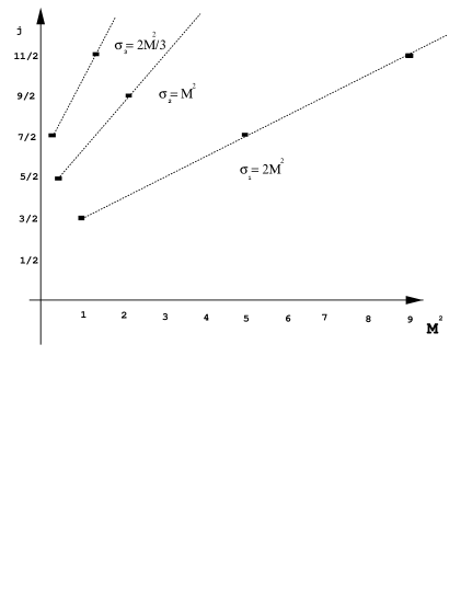
Figure 7: The spectrum of $\Gamma^{-2}_{0}$ has a structure of linear trajectories with different string tension $2\pi\sigma_{n}=2M^{2}/n,~{}~{}n=1,2,..$. The smallest mass on a given trajectory $n$ has the spin $j=n+1/2$ and tends to zero as $1/n^{2}$.

The other solution, $\Sigma_{2}$-solution, which shares the above properties of $\Sigma_{1}$-solution is (119) with

$$\gamma^{1~{}2}_{j}~{}=~{}\gamma^{3~{}4}_{j}~{}=....=0~{}~{}~{}~{}~{}~{}\gamma^{\dot{1}~{}\dot{2}}_{j}~{}=~{}\gamma^{\dot{3}~{}\dot{4}}_{j}~{}=...=0.$$ (143)

The difference between the last two solutions is that in the first case the lower spin is $j=3/2$ and in the second case it is $j=1/2$. The unwanted property of all these solutions $\Sigma$, $\Sigma_{1}$ and $\Sigma_{2}$ is that the smallest mass $M^{2}_{n}(min)$ tends to zero as it was in the original Majorana equation and the spectrum is not bounded from bellow. It is also true that $\Sigma=\Sigma_{1}+\Sigma_{2}$ in the sense of the footnote 5.

We have to remark also that both equations, $\Sigma_{1}$ and $\Sigma_{2}$, which correspond to (134) and to (143) have natural $constraints$. In the rest frame they are

$$\left(\begin{array}[]{c}\psi_{1}\\ \psi_{\dot{1}}\end{array}\right)_{1/2}=\left(\begin{array}[]{c}\psi_{3}\\ \psi_{\dot{3}}\end{array}\right)_{5/2}=.....=\left(\begin{array}[]{c}\psi_{2k-1}\\ \psi_{\dot{2k-1}}\end{array}\right)_{(4k-3)/2}~{}=~{}0~{}~{}~{}~{}k=1,2,...$$ (144)

for the $\Sigma_{1}$ case (134) and are

$$\left(\begin{array}[]{c}\psi_{2}\\ \psi_{\dot{2}}\end{array}\right)_{3/2}=\left(\begin{array}[]{c}\psi_{4}\\ \psi_{\dot{4}}\end{array}\right)_{7/2}=.....=\left(\begin{array}[]{c}\psi_{2k}\\ \psi_{\dot{2k}}\end{array}\right)_{(4k-1)/2}~{}=~{}0~{}~{}~{}~{}k=1,2,...$$ (145)

for the $\Sigma_{2}$ case (143). We shall return to this constraints with more details in the second part of this article.

10 The $\Gamma_{5}$ mass term

One can define the $\Gamma_{5}$ matrix which has all the properties of Dirac’s $\gamma_{5}$ matrix (see Appendix C)    $\{\Gamma_{5},\Gamma_{\mu}\}=0$ and allows to introduce an additional mass term into the string equation (49) of the form

$$(\vec{a}\cdot\vec{b})~{}\Gamma_{5}.$$

It was our aim to use the representations $\Theta$ of the Lorentz group which have nonzero Casimir operator

$$<j,m,r~{}|~{}\vec{a}\cdot\vec{b}~{}|~{}r,j,m>=~{}i~{}\lambda~{}(r-1/2)$$

$$<j,m,\dot{r}~{}|~{}\vec{a}\cdot\vec{b}~{}|~{}\dot{r},j,m>=-i~{}\lambda~{}(r-1/2).$$

The matrix $(\vec{a}\cdot\vec{b})~{}\Gamma_{5}$ is diagonal

$$<j,m,r~{}|(\vec{a}\cdot\vec{b})~{}\Gamma_{5}|~{}r,j,m>~{}=~{}<j,m,\dot{r}~{}|(\vec{a}\cdot\vec{b})~{}\Gamma_{5}|~{}\dot{r},j,m>$$

$$=i~{}\lambda~{}M~{}(-1)^{r+1}(r-1/2).$$

With this new mass term the mass spectrum of the theory changes and we get trajectory

$$M^{2}_{1}=2M^{2}~{}(j-1)\cdot\lambda^{2}j(j+1)\approx 2(\lambda M)^{2}j^{3},$$

thus for this trajectory

$$2\pi\sigma_{1}=\frac{1}{\alpha^{{}^{\prime}}_{1}}=2(\lambda M)^{2}\cdot j^{2}.$$

For the second and third trajectories we have

$$M^{2}_{2}=M^{2}\frac{(j^{2}-3j+2)}{(j-1/2)}\cdot\lambda^{2}(j-1)j\approx(\lambda M)^{2}j^{3},$$

$$M^{2}_{3}=\frac{2M^{2}}{3}\frac{(j^{2}-5j+6)}{(j-1)}\cdot\lambda^{2}(j-2)(j-1)\approx\frac{2(\lambda M)^{2}}{3}j^{3},$$

thus

$$2\pi\sigma_{2}=\frac{1}{\alpha^{{}^{\prime}}_{2}}=(\lambda M)^{2}\cdot j^{2}~{}~{}~{}~{}~{}~{}~{}~{}~{}~{}~{}~{}~{}2\pi\sigma_{3}=\frac{1}{\alpha^{{}^{\prime}}_{3}}=2(\lambda M)^{2}/3\cdot j^{2},$$ (146)

and so on. The appearance of $\lambda$ in these formulas together with $M$ demonstrates that this contribution to the spectrum is possible only if we use representations which have nonzero Casimir operators. The general formula for all trajectories is

$$M^{2}_{n}=\frac{2(\lambda M)^{2}}{n}\frac{j^{2}-(2n-1)j+n(n-1)}{j-(n-1)/2}(j+1-n)(j+2-n)~{}~{}~{}~{}n=1,2,...$$ (147)

and the smallest mass on a given trajectory behaves as

$$M^{2}_{n}(j=n+1/2)=\frac{3(\lambda M)^{2}}{n(n+3)}~{}\frac{3}{2}~{}\frac{5}{2}~{}~{}~{}~{}~{}~{}~{}j=n+1/2$$

and still falls down as $1/n^{2}$.

11 The dual string equation

Under the dual transformation (23)

$$\Theta=(j_{0};\lambda)\rightarrow(\lambda;j_{0})=\Theta^{dual}$$

the representation $\Theta$ (85) is transformed into its dual

$$.....(\lambda;-5/2)~{}~{}(\lambda;-3/2)~{}~{}(\lambda;-1/2)~{}~{}(\lambda;1/2)~{}~{}(\lambda;3/2)~{}~{}(\lambda;5/2)....$$ (148)

and we shall consider here the case $\lambda=1/2$ in order to have the Dirac representation incorporated in $\Theta$. The solution which is dual to $\Sigma_{2}$ (119) and (143) is equal to

$$\gamma^{r+1~{}r}_{j}=~{}\gamma^{r~{}r+1}_{j}=\gamma^{\dot{r+1}~{}\dot{r}}_{j}=\gamma^{\dot{r}~{}\dot{r+1}}_{j}=\sqrt{(\frac{1}{4}-\frac{j^{2}+j}{4r^{2}-1})}~{}~{}~{}~{}~{}r\geq j+3/2$$ (149)

where $j=1/2,3/2,5/2,...$,  $r=2,4,6,....$ and the rest of the elements are equal to zero

$$\gamma^{\dot{1}~{}1}~{}=~{}\gamma^{1~{}2}_{j}~{}=~{}\gamma^{3~{}4}_{j}=....=0~{}~{}~{}~{}~{}\gamma^{1~{}\dot{1}}~{}=~{}\gamma^{\dot{1}~{}\dot{2}}~{}=~{}\gamma^{\dot{3}~{}\dot{4}}~{}=...=0.$$ (150)

The Lorentz boost operators $\vec{b}$ are antihermitian in this case

$$b^{+}_{k}=-b_{k},$$ (151)

because the amplitudes $\varsigma$ (22) are pure imaginary and therefore the $\Gamma_{k}$ matrices are also antihermitian

$$\Gamma^{+}_{k}=-\Gamma_{k}.$$ (152)

The matrix $\Omega$ changes and is now equal to the parity operator $P$, the relation

$$\Omega~{}\Gamma^{+}_{\mu}=\Gamma_{\mu}~{}\Omega$$

remains valid. The diagonal part of $\Gamma_{k}$ anticommutates with $\Gamma_{0}$ as it was before (135)

$$\{\Gamma_{0},\tilde{\Gamma_{k}}\}=0~{}~{}~{}~{}~{}~{}~{}~{}k=x,y,z$$ (153)

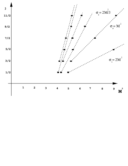
Figure 8: The spectrum of the dual equation has again a structure of linear trajectories with string tension $2\pi\sigma_{n}=2M^{2}/n,~{}~{}n=1,2,..$. The smallest mass on a given trajectory $n$ has the spin $j=1/2$ or $j=3/2$ and is bounded from bellow.

The mass spectrum is equal to

$$M^{2}_{n}=\frac{2M^{2}}{n}~{}\frac{(j+n)(j+n+1)}{j+(n+1)/2}$$ (154)

where $n=1,2,3,..$ and enumerates the trajectories (see Figure 8). The lower spin on a given trajectory is either $1/2$ or $3/2$ depending on n: if n is odd then $j_{min}=1/2$, if n is even then $j_{min}=3/2$. This is an essential new property of the dual equation because now we have an infinite number of states with a given spin $j$ instead of $j+1/2$, which we had before we did the dual transformation. The string tension is the same as in the dual system (141)

$$2\pi\sigma_{n}=\frac{2M^{2}}{n}~{}~{}~{}~{}~{}~{}~{}~{}~{}~{}~{}~{}~{}~{}n=1,2,3,...$$ (155)

and the lower mass on a given trajectory $n$ is given by the formula $(j=1/2)$

$$M^{2}_{n}(j=1/2)=\frac{4M^{2}}{n}\frac{(2n+1)(2n+3)}{n+2}\rightarrow(4M)^{2}.$$ (156)

Thus the main problem of decreasing spectrum has been solved after the dual transformation because the spectrum is now bounded from below.

Including the $\Gamma_{5}$ mass term one can see that all trajectories acquire a nonzero slope

$$M^{2}_{n}=\frac{2M^{2}}{n}~{}\frac{(j+n)^{2}(j+n+1)^{2}}{j+(n+1)/2}\frac{1}{4}$$ (157)

where

$$n=1,2,3,....$$

$$j(n)_{min}=1/2,3/2,1/2,....$$

thus for the lower mass on a given trajectory $n$ we have

$$M^{2}_{n}(j=1/2)=\frac{M^{2}}{16}\frac{(2n+1)^{2}(2n+3)^{2}}{n(n+2)}\rightarrow M^{2}n^{2}.$$ (158)

Turning on the pure Casimir mass term $gM~{}(\vec{a}^{2}-\vec{b}^{2})$ we will get the spectrum which grows as $j^{5}$

$$M^{2}_{n}=g^{2}~{}\frac{2M^{2}}{n}\frac{(j+n)^{3}(j+n+1)^{3}}{j+(n+1)/2},$$ (159)

where $n=1,2,3...$

12 Extension to bosons

Irrespective of the future interpretation of the theory it is important to include bosons. The appropriate representation $\Theta$ for this purpose is

$$.....(\lambda;-3)~{}~{}(\lambda;-2)~{}~{}(\lambda;-1)~{}~{}(\lambda;0)~{}~{}~{}~{}~{}(\lambda;0)~{}~{}(\lambda;1)~{}~{}(\lambda;2)~{}~{}(\lambda;3)....$$ (160)

and we shall consider $\lambda=0$. The solution for $\Gamma_{0}$ is of the same form as we had before for fermions

$$\gamma^{r+1~{}r}_{j}=~{}\gamma^{r~{}r+1}_{j}=\gamma^{\dot{r+1}~{}\dot{r}}_{j}=\gamma^{\dot{r}~{}\dot{r+1}}_{j}=\sqrt{(\frac{1}{4}-\frac{j^{2}+j}{4r(r-1)})}~{}~{}~{}~{}~{}r\geq j+2$$ (161)

where $j=0,1,2,3,..$,  $r=2,4,6,....$ and the rest of the elements are equal to zero

$$\gamma^{\dot{1}~{}1}~{}=~{}\gamma^{1~{}2}_{j}~{}=~{}\gamma^{3~{}4}_{j}=....=0~{}~{}~{}~{}~{}\gamma^{1~{}\dot{1}}~{}=~{}\gamma^{\dot{1}~{}\dot{2}}~{}=~{}\gamma^{\dot{3}~{}\dot{4}}~{}=...=0.$$ (162)

One can compute the slope of the first trajectory

$$M^{2}_{1}=2M^{2}~{}(j+2)\approx 2M^{2}j,~{}~{}~{}~{}~{}~{}~{}~{}~{}~{}j=0,2,4,...$$ (163)

thus for this trajectory the string tension $\sigma$ is equal to

$$2\pi\sigma_{1}=\frac{1}{\alpha^{{}^{\prime}}_{1}}=2M^{2}$$ (164)

and coincides with the one we obtain for the fermion string. The general formula for the mass spectrum is

$$M^{2}_{n}=\frac{2M^{2}}{n}\frac{(j+n)(j+n+1)}{j+(n+1)/2}~{}~{}~{}~{}~{}n=1,2,3,...$$ (165)

and the lower spin on a given trajectory is either $0$ or $1$ depending on n: if n is odd then $j_{min}=0$, if n is even then $j_{min}=1$. Comparing this spectrum with the fermionic one (154) one can see that fermions and bosons lie on the same trajectories. In the bosonic case we do not have $\Gamma_{5}$-matrix and the Casimir operator $(\vec{a}\cdot\vec{b})$ is zero because $\lambda=0$, but we can include pure Casimir mass term $(\vec{a}^{2}-\vec{b}^{2})$ into the string equation to receive additional contribution to the slope of the trajectories. The formula for the spectrum is the same as for the fermions (159).

13 Discussion

In this article we suggest a relativistic equation for the gonihedric string which has the Dirac form. The spectrum of the theory consists of particles and antiparticles of increasing half-integer spin lying on quasilinear trajectories of different slope. Explicit formulas for the mass spectrum allow to compute the string tension and thus demonstrate the string character of the theory. The old problem of decreasing mass spectrum has been solved and the spectrum is bounded from below. The trajectories are only asymptotically linear and thus are different from the free string linear trajectories. It is difficult to say at the moment what is the physical reason for this nonperturbative behaviour. Nonzero Casimir operators and the generalization of the $\Gamma_{5}$ matrix allow to introduce additional mass terms into the string equation and to increase the slope of the trajectories.

The equation is explicitly Lorentz invariant, but what we have now to worry about is the unitarity of the theory and unwanted ghost solutions. In the second part of this article we shall return to these questions and will demonstrate that tachyonic solutions which appear in Majorana equation do not show up here. This is because the nondiagonal transition amplitudes of the form $<..j..|~{}\Gamma_{k}~{}|j\pm 1>$ are small here and the diagonal amplitudes $<..j..|~{}\Gamma_{k}~{}|j>$ are large. Indeed in the Majorana equation the diagonal elements are equal to zero, therefore the nondiagonal elements give rise to space-like tachyonic solutions (see (20) in [2]). In the Dirac equation only diagonal transition amplitudes are present, and so the equation does not admit tachyonic solutions. The problem of ghost states is more subtle here and we shall analyze the natural constraints appearing in the system in the second part of this article to ensure that they decouple from the physical space of states.

In conclusion one of us (G.K.S.) wishes to acknowledge the hospitality of the Niels Bohr Institute where this work was started and would like to thank J.Ambjorn, P.Olesen, G.Tiktopoulos and P.Di Vecchia for the interesting discussions. We are thankful to Pavlos Savvidis, who has found the recurrent relation for the computation of the characteristic polynomials of the Jacoby matrices which finally leads to the basic solution for $\Gamma_{0}$. This work has been initiated during Triangular Meeting in Rome, in March 1996, where we got the collected articles of Ettore Majorana: ”La vita e l’opera di Ettore Majorana (1906-1938)” Roma, Accademia Nazionale dei Lincei, 1966, (ed. by E. Amaldi).

Figure 9: Surface $M_{2}$ degenerates into a single world line $M_{1}$ and the action $A(M_{2})$ is reduced to the length of the world line $L(M_{1})$.

14 Appendix A

Jacoby matrices.   We are searching for the solution of equations (57) in the form of Jacoby matrices

$$\left(\begin{array}[]{c}0,~{}~{}a\\ a,~{}~{}0\end{array}\right),~{}~{}\left(\begin{array}[]{c}0,~{}~{}b,{}{}{}{}{}{}{}\\ b,~{}~{}0,~{}~{}a,{}{}{}\\ ~{}~{}~{}~{}a,~{}~{}0,~{}~{}b\\ ~{}~{}~{}~{}~{}~{}~{}~{}b,~{}~{}0\end{array}\right),~{}~{}\left(\begin{array}[]{c}0,~{}~{}c,{}{}{}{}{}{}{}{}{}{}{}{}{}{}{}\\ c,~{}~{}0,~{}~{}b,{}{}{}{}{}{}{}{}{}{}{}\\ ~{}~{}~{}~{}b,~{}~{}0,~{}~{}a,{}{}{}{}{}{}{}\\ ~{}~{}~{}~{}~{}~{}~{}~{}a,~{}~{}0,~{}~{}b,{}{}{}\\ ~{}~{}~{}~{}~{}~{}~{}~{}~{}~{}~{}~{}b,~{}~{}0,~{}~{}c\\ ~{}~{}~{}~{}~{}~{}~{}~{}~{}~{}~{}~{}~{}~{}~{}~{}c,~{}~{}~{}0\end{array}\right),....$$ (166)

The characteristic polynomials have the form

$$x^{2}-a^{2}=0$$

$$x^{4}-(a^{2}+2b^{2})x^{2}+b^{4}=0$$

$$x^{6}-(a^{2}+2b^{2}+2c^{2})x^{4}+(2a^{2}c^{2}+2b^{2}c^{2}+b^{4}+c^{4})x^{2}-a^{2}c^{4}=0$$

$$x^{8}-(a^{2}+2b^{2}+2c^{2}+2d^{2})x^{6}+~{}~{}~{}~{}$$ (167)

$$(2a^{2}c^{2}+2b^{2}c^{2}+2a^{2}d^{2}+2c^{2}d^{2}+b^{4}+c^{4}+d^{4}+4b^{2}d^{2})x^{4}-~{}~{}~{}~{}$$

$$-(a^{2}c^{4}+a^{2}d^{4}+2b^{2}d^{4}+2b^{4}d^{2}+2a^{2}c^{2}d^{2}+2b^{2}c^{2}d^{2})x^{2}+b^{4}d^{4}=0$$

$$.~{}.~{}.~{}.~{}.~{}.~{}.~{}.~{}.~{}.~{}.~{}.~{}.~{}.~{}.~{}.~{}.~{}.~{}.~{}.~{}.~{}.~{}.~{}.~{}.~{}.~{}.~{}.~{}.~{}.~{}.~{}.$$

15 Appendix B

$\sigma$ and $\tau$ algebra.  j=1/2

$$\sigma_{1/2}=0$$

j=3/2 For this spin we have

$$\sigma_{3/2},~{}~{}\sigma^{*}_{3/2},~{}~{}\sigma^{2}_{3/2}~{}=~{}\sigma^{*~{}2}_{3/2}=0$$

and the main relation is

$$\sigma_{3/2}~{}\sigma^{*}_{3/2}+\sigma^{*}_{3/2}~{}\sigma_{3/2}=4$$

and thus

$$\gamma_{3/2}=\omega_{3/2}(1+\sigma_{3/2})$$ (169)

j=5/2 For this spin we have

$$\sigma_{5/2},~{}\sigma^{*}_{5/2},~{}\sigma^{2}_{5/2},~{}\sigma^{*~{}2}_{5/2},~{}~{}\sigma^{3}_{5/2}~{}=~{}\sigma^{*~{}3}_{5/2}~{}=0$$

which appears to satisfy the algebra

$$\{\sigma_{5/2},~{}\sigma^{*}_{5/2}\}-2~{}(\sigma_{5/2}+\sigma_{5/2})-3~{}\{\sigma^{2}_{5/2},~{}\sigma^{*~{}2}_{5/2}\}+4~{}(\sigma^{2}_{5/2}+\sigma^{*~{}2}_{5/2})=2$$ (171)

Then it follows that

$$\gamma_{5/2}=\omega_{5/2}(1+\sigma_{5/2})$$

and that

$$\sigma^{2}_{5/2}~{}\sigma^{*~{}2}_{5/2}~{}\sigma^{2}_{5/2}=2~{}\sigma^{2}_{5/2}~{}\sigma^{*}_{5/2}~{}\sigma^{2}_{5/2}.$$ (173)

Similar algebra takes place for the $\tau_{j}$ matrices.

16 Appendix C

Parity and $\Gamma_{5}$ matrices.  The commutation relations which define the parity operator P are

$$P~{}a_{k}=a_{k}~{}P~{}~{}~{}~{}~{}P~{}b_{k}=-b_{k}~{}P~{}~{}~{}~{}~{}P^{2}=1,$$ (174)

because the parity operator P commutes with spatial rotations we have

$$P=P^{rr^{\prime}}_{j}~{}\delta_{jj^{\prime}}~{}\delta_{mm^{\prime}}$$ (175)

and from the second commutator

$$P^{r\dot{r}}_{j}=-P^{r\dot{r}}_{j-1}~{}~{}~{}~{}P^{\dot{r}r}_{j}=-P^{\dot{r}r}_{j-1},$$ (176)

thus

$$P^{r\dot{r}}_{j}=P^{\dot{r}r}_{j}=(-1)^{[j]}$$ (177)

One can check that

$$P~{}\Gamma_{0}=\Gamma_{0}~{}P~{}~{}~{}~{}~{}P~{}\Gamma_{k}=-\Gamma_{k}~{}P~{}~{}~{}~{}~{}~{}~{}P~{}\Omega=\Omega~{}P$$ (178)

$$P_{1/2}=\left(\begin{array}[]{c}0,~{}1\\ 1,~{}0\end{array}\right),~{}~{}P_{3/2}=\left(\begin{array}[]{c}~{}~{}~{}~{}~{}~{}~{}~{}~{}-1\\ ~{}~{}~{}~{}~{}~{}-1{}{}\\ ~{}~{}~{}-1{}{}{}{}{}\\ -1{}{}{}{}{}{}{}{}\end{array}\right),~{}~{}P_{5/2}=\left(\begin{array}[]{c}~{}~{}~{}~{}~{}~{}~{}~{}~{}~{}~{}~{}1\\ ~{}~{}~{}~{}~{}~{}~{}~{}~{}1{}{}\\ ~{}~{}~{}~{}~{}~{}1{}{}{}{}{}\\ ~{}~{}~{}1{}{}{}{}{}{}{}{}\\ ~{}~{}1{}{}{}{}{}{}{}{}{}{}\\ 1{}{}{}{}{}{}{}{}{}{}{}{}{}\end{array}\right),...$$ (179)

For $\Gamma_{5}$ we have

$$\Gamma_{5}~{}a_{k}=a_{k}~{}\Gamma_{5}~{}~{}~{}~{}~{}\Gamma_{5}~{}b_{k}=b_{k}~{}\Gamma_{5}~{}~{}~{}~{}~{}~{}~{}~{}~{}\Gamma_{5}^{2}=1$$ (180)

because it commutes with spatial rotations we have

$$\Gamma_{5}=\Gamma_{5~{}j}^{rr^{\prime}}~{}\delta_{jj^{\prime}}~{}\delta_{mm^{\prime}}$$ (181)

and from the second commutator

$$\Gamma_{5~{}j}^{rr}=\Gamma_{5~{}j-1}^{rr}~{}~{}~{}~{}\Gamma_{5~{}j}^{\dot{r}\dot{r}}=\Gamma_{5~{}j-1}^{\dot{r}\dot{r}}~{}~{}~{}~{}\Gamma_{5~{}j}^{rr}=-\Gamma_{5~{}j}^{\dot{r}\dot{r}}$$ (182)

thus

$$\Gamma_{5~{}j}^{rr}=-\Gamma_{5~{}j}^{\dot{r}\dot{r}}=(-1)^{r+1}$$ (183)

One can check that

$$\Gamma_{5}~{}\Gamma_{0}=-\Gamma_{0}~{}\Gamma_{5}~{}~{}~{}~{}~{}\Gamma_{5}~{}\Gamma_{k}=-\Gamma_{k}~{}\Gamma_{5}~{}~{}~{}~{}~{}~{}~{}\Gamma_{5}~{}P=-P~{}\Gamma_{5}~{}~{}~{}~{}~{}~{}\Gamma_{5}~{}\Omega=-\Omega~{}\Gamma_{5}$$ (184)

and thus

$$\Gamma_{5~{}1/2}=\left(\begin{array}[]{c}1{}{}\\ ~{}~{}~{}-1\end{array}\right),~{}~{}\Gamma_{5~{}3/2}=\left(\begin{array}[]{c}-1,{}{}{}{}{}{}{}\\ ~{}~{}~{}1,{}{}{}{}\\ ~{}~{}~{}~{}~{}~{}-1{}{}\\ ~{}~{}~{}~{}~{}~{}~{}~{}~{}1\end{array}\right),~{}~{}\Gamma_{5~{}5/2}=\left(\begin{array}[]{c}1{}{}{}{}{}{}{}{}{}{}{}{}\\ ~{}~{}-1{}{}{}{}{}{}{}{}{}\\ ~{}~{}~{}~{}~{}1{}{}{}{}{}{}{}\\ ~{}~{}~{}~{}~{}~{}~{}-1{}{}{}{}\\ ~{}~{}~{}~{}~{}~{}~{}~{}~{}~{}1{}{}\\ ~{}~{}~{}~{}~{}~{}~{}~{}~{}~{}~{}~{}-1\end{array}\right),...$$ (185)

17 Appendix D

Hermitian solution of $\Gamma_{0}$ for finite N.  The Hermitian solution of (57) for the $\Gamma_{0}$ can be constructed by using our previous solution

$$\gamma^{r+1~{}r}_{j}=-\gamma^{r~{}r+1}_{j}=-\gamma^{\dot{r+1}~{}\dot{r}}_{j}=\gamma^{\dot{r}~{}\dot{r+1}}_{j}=i~{}\sqrt{(1-\frac{r^{2}}{N^{2}})~{}(\frac{j^{2}+j}{4r^{2}-1}-\frac{1}{4})}~{}~{}~{}~{}~{}j\geq r+1/2$$ (186)

$$\gamma^{1~{}\dot{1}}_{j}=\gamma^{\dot{1}~{}1}_{j}=j+1/2$$ (187)

which for the low values of $j$ is:

$$\gamma_{1/2}=\left(\begin{array}[]{c}0,~{}~{}~{}~{}~{}~{}1\\ 1,~{}~{}~{}~{}~{}~{}0\end{array}\right),~{}~{}\gamma_{3/2}=\left(\begin{array}[]{c}0,~{}~{}~{}~{}~{}~{}~{}~{}~{}~{}~{}~{}~{}i\sqrt{1-1/N^{2}},{}{}{}{}{}{}{}{}{}{}{}{}{}{}{}{}{}{}{}{}{}{}{}\\ -i\sqrt{1-1/N^{2}},~{}~{}~{}~{}~{}0,~{}~{}~{}~{}~{}~{}2,{}{}{}{}{}{}{}{}{}{}{}{}{}{}{}{}{}{}{}{}{}{}{}\\ ~{}~{}~{}~{}~{}~{}~{}~{}~{}~{}~{}~{}~{}~{}~{}~{}~{}~{}~{}~{}~{}~{}~{}~{}2,~{}~{}~{}~{}~{}~{}0,~{}~{}~{}~{}~{}~{}~{}~{}~{}~{}i\sqrt{1-1/N^{2}}\\ ~{}~{}~{}~{}~{}~{}~{}~{}~{}~{}~{}~{}~{}~{}~{}~{}~{}~{}~{}~{}~{}~{}~{}~{}~{}~{}~{}~{}-i\sqrt{1-1/N^{2}},~{}~{}~{}~{}~{}~{}~{}~{}~{}~{}~{}0\end{array}\right),$$

$$\gamma_{5/2}=\left(\begin{array}[]{c}0,~{}~{}~{}~{}~{}~{}i\sqrt{(1-4/N^{2})(1/3)},{}{}{}{}{}{}{}{}{}{}{}{}{}{}{}{}{}{}{}{}{}{}\\ -i\sqrt{(1-4/N^{2})(1/3)},~{}~{}~{}~{}~{}0,~{}~{}~{}~{}~{}~{}~{}~{}~{}~{}i\sqrt{(1-1/N^{2})(8/3)},{}{}{}{}{}{}{}{}{}{}{}{}{}{}{}{}{}\\ ~{}~{}~{}~{}~{}~{}~{}~{}~{}~{}~{}~{}~{}-i\sqrt{(1-1/N^{2})(8/3)},~{}~{}~{}~{}0,~{}~{}~{}~{}~{}~{}~{}~{}~{}~{}3,{}{}{}{}{}{}{}\\ ~{}~{}~{}~{}~{}~{}~{}~{}~{}~{}~{}~{}~{}~{}~{}~{}~{}~{}~{}~{}~{}~{}~{}~{}~{}~{}~{}~{}~{}~{}~{}~{}~{}~{}~{}~{}~{}~{}~{}~{}~{}3,~{}~{}~{}~{}~{}~{}~{}~{}~{}~{}0,~{}~{}~{}~{}~{}i\sqrt{(1-1/N^{2})(8/3)},{}{}{}{}{}{}{}{}{}\\ ~{}~{}~{}~{}~{}~{}~{}~{}~{}~{}~{}~{}~{}~{}~{}~{}~{}~{}~{}~{}~{}~{}~{}~{}~{}~{}-i\sqrt{(1-1/N^{2})(8/3)},~{}~{}~{}0,~{}~{}~{}i\sqrt{(1-4/N^{2})(1/3)}\\ ~{}~{}~{}~{}~{}~{}~{}~{}~{}~{}~{}~{}~{}~{}~{}~{}~{}~{}~{}~{}~{}~{}~{}~{}~{}~{}~{}~{}~{}~{}~{}~{}~{}~{}~{}~{}~{}~{}~{}-i\sqrt{(1-4/N^{2})(1/3)},~{}~{}~{}0\end{array}\right),$$

$$etc...$$

The characteristic equations for these matrices are:

$$\gamma^{2}_{1/2}-1=0,$$

$$(\gamma^{2}_{3/2}-2\gamma_{3/2}-1+1/N^{2})~{}(\gamma^{2}_{3/2}+2\gamma_{3/2}-1+1/N^{2})=0,$$

$$(\gamma^{3}_{5/2}+3\gamma^{2}_{5/2}-3\gamma_{5/2}-1+4(\gamma_{5/2}+1)/N^{2})~{}~{}~{}~{}$$

$$(\gamma^{3}_{5/2}-3\gamma^{2}_{5/2}-3\gamma_{5/2}+1+4(\gamma_{5/2}-1)/N^{2})=0,$$

$$............................................................$$

and the eigenvalues $\epsilon_{j}$ can be found

$$1~{}~{}~{}~{}~{}~{}~{}~{}~{}~{}~{}~{}~{}~{}~{}~{}~{}~{}~{}~{}~{}~{}~{}~{}~{}~{}~{}~{}~{}j=1/2$$

$$\sqrt{2-1/N^{2}}-1~{}~{}~{}~{}~{}~{}~{}~{}\sqrt{2-1/N^{2}}+1~{}~{}~{}~{}~{}~{}~{}~{}~{}~{}~{}~{}~{}~{}~{}~{}~{}~{}~{}~{}~{}~{}~{}~{}~{}~{}~{}~{}j=3/2$$

$$.~{}.~{}.~{}.~{}.~{}.~{}.~{}.~{}.~{}.~{}.~{}.~{}.~{}.~{}.~{}.~{}.~{}.~{}.~{}.~{}.~{}.~{}.~{}.~{}.~{}.~{}.~{}.~{}.~{}.~{}.~{}.~{}.~{}.~{}.~{}.~{}.~{}.~{}.~{}.~{}.~{}.~{}.~{}.~{}.~{}~{}~{}~{}~{}~{}~{}~{}~{}~{}~{}~{}~{}~{}$$

When $N\rightarrow\infty$ these formulas are reduced to the formulas presented in the section where we consider the Hermitian solution.

18 Appendix E

Nonzero Casimir operators.   If $\lambda=0$ then

$$<\vec{a}\cdot\vec{b}>=0~{}~{}~{}<(\vec{a}^{2}-\vec{b}^{2})>=(r-1/2)^{2}-1$$

and

$$\varsigma^{r}_{j}=\varsigma^{\dot{r}}_{j}=\frac{1}{2}\sqrt{1-(\frac{r^{2}-r}{j^{2}-1/4})}~{}~{}~{}~{}~{}~{}j\geq r+1/2.$$

and if $\lambda=1$ then

$$<\vec{a}\cdot\vec{b}>=i~{}(r-1/2)~{}~{}~{}~{}~{}<(\vec{a}^{2}-\vec{b}^{2})>=(r-1/2)^{2}$$

An essential simplification appears when $\lambda=1/2$, in that case

$$\varsigma^{r}_{j}=\varsigma^{\dot{r}}_{j}=\frac{1}{2}\sqrt{1-(\frac{r-1/2}{j})^{2}}~{}~{}~{}~{}~{}~{}j\geq r+1/2$$

and

$$<\vec{a}\cdot\vec{b}>=i/2~{}(r-1/2)~{}~{}~{}~{}~{}<(\vec{a}^{2}-\vec{b}^{2})>=(r-1/2)^{2}-3/4.$$

References

- [1] P.A.M.Dirac. The Quantum Theory of Electron. Proc.Roy.Soc. A117 (1928) 610; A118 (1928) 351
- [2] E.Majorana. Teoria Relativistica di Particelle con Momento Intrinseco Arbitrario. Nuovo Cimento 9 (1932) 335
- [3] P.Ramond. Dual Theory for Free Fermions. Phys.Rev. D3 (1971) 2415
-
[4]
P.A.M.Dirac. Relativistic wave equations.
Proc.Roy.Soc. A155 (1936) 447;
Unitary Representation of the Lorentz Group. Proc.Roy.Soc. A183 (1944) 284
M.Fierz and W.Pauli. On Relativistic Wave Equations for Particles of Arbitrary Spin in an Electromagnetic Field. Proc.Roy.Soc. A173 (1939) 211
W.Rarita and J.Schwinger. On a Theory of Particles with Half-Integral Spin. Phys.Rev. 60 (1941) 61
I.M.Gel’fand and M.A.Naimark. J.Phys. (USSR) 10 (1946) 93
I.M.Gel’fand and A.M.Yaglom. Zh.Experim. i Teor.Fiz. 18 (1948) 707
Y.Nambu. Phys.Rev. 160 (1967) 1171
W.Rúhl. Comm.Math.Phys. 6 (1967) 312 -
[5]
Superstrings: the first 15 years of superstring theory.
V1,V2. World Scientific 1985. (Ed. by J.Schwarz)
M.Green, J.Schwarz and E.Witten. Superstring Theory. V1,V2. Cambridge University Press, Cambridge, 1988
J.Polchinski. TASI Lectures on D-Branes. NSF-ITP-96-145; hep-th/9611050
T.Banks,W.Fischler,S.H.Shenker and L.Susskind. M-theory as a Matrix Model: A Conjecture, hep-th/9610043
C. Bachas, Introduction to D-branes, hep-th/9701019 -
[6]
H.B.Nielsen and P.Olesen. Phys.Lett. B32 (1970) 203
D.J.Gross and F.Wilczek. Phys.Rev.Lett.30(1973)1343
H.D.Politzer. Phys.Rev.Lett.30(1973)1346
K.Wilson. Phys.Rev.D10 (1974) 2445
G. ’t Hooft. Nucl.Phys. B72 (1974) 461; Nucl.Phys. B75 (1975) 461
G.K.Savvidy. Phys.Lett. B71 (1977) 133
A.Polyakov. Gauge fields and String. (Harwood Academic Publishers, 1987)
D.Gross and W.Taylor. Nucl.Phys. B400 (1993) 181 ; B403 (1993) 395
N. Seiberg and E. Witten. Nucl.Phys.B426 (1994) 19; Nucl.Phys.B431 (1994) 484 -
[7]
G.K. Savvidy and K.G. Savvidy. Gonihedric string and
asymptotic freedom. Mod.Phys.Lett. A8 (1993) 2963
R.V. Ambartzumian, G.K. Savvidy , K.G. Savvidy and G.S. Sukiasian. Phys. Lett. B275 (1992) 99
G.K. Savvidy and K.G. Savvidy. Int. J. Mod. Phys. A8 (1993) 3993. - [8] G.K.Savvidy and R.Schneider. Comm.Math.Phys. 161 (1994) 283
- [9] B.Durhuus and T.Jonsson. Phys.Lett. B297 (1992) 271
-
[10]
G.K.Savvidy. Symplectic and large-N gauge theories.
In ”Cargese 1990,v.225, Proceedings, Vacuum structure in intense fields”.
Plenum Press, NY 1991, p415
Renormalization of infinite dimensional gauge symmetries. (Minnesota U. and Yerevan Phys. Inst.). TPI-MINN-90-2-T, Jan 1990. 18pp. -
[11]
M.Born, W.Heisenberg and P.Jordan. Z.Physik 35 (1926) 557
H.Weyl. Math.Z. 24 (1926) 342
H.Weyl. The theory of groups and quantum mechanics. London. Methuen 1931.
R.Brauer and H.Weyl. Amer.J.Math. 57 (1935) 425
E.Cartan. Bull.Soc.math.France 41 (1913) 53
Van der Waerden. Die gruppentheoretische methode der Quantummechanik. Berlin, Springer 1932; Nachr.Ges.Wiss.Gott. (1929) 100
E.P.Wigner. Ann.Math. 40 (1939) 149; Z.Physik. 124 (1948) 665
O.Laporte and G.Uhlenbeck. Phys.Rev. 37 (1931) 1380 - [12] G.K.Savvidy and F.J.Wegner. Nucl.Phys.B413(1994)605.
- [13] G.K. Savvidy and K.G. Savvidy. Phys.Lett. B324 (1994) 72
- [14] G.K. Savvidy and K.G. Savvidy. Interaction hierarchy. Phys.Lett. B337 (1994) 333; Mod.Phys.Lett. A11 (1996) 1379.
- [15] R. Pietig and F.J. Wegner. Nucl.Phys. B466 (1996) 513
- [16] M.Creutz, Quarks, gluons and lattices. (Cambridge University Press,Cambridge 1983)
- [17] C.F.Baillie and D.A.Johnston. Phys.Rev D 45 (1992) 3326
-
[18]
G.Koutsoumbas, G.K. Savvidy and K.G. Savvidy.
Phase structure of four-dimensional gonihedric spin sysytem.
Phys.Lett. B (1997); hep-th/9706173
G.K.Bathas et.al. Mod.Phys.Lett. A10 (1995) 2695 - [19] G.K.Savvidy. Classical and quantum mechanics of nonabelian gauge fields. Nucl.Phys. B246 (1984) 302