VARIOUS SHADES OF BLUE’S FUNCTIONS

Romuald A. Janik¹, Maciej A. Nowak^1,2,3, Gábor Papp^2,4, and
Ismail Zahed⁵

¹Department of Physics, Jagellonian University, 30-059 Kraków, Poland
²GSI, Planckstr. 1, D-64291 Darmstadt, Germany
³Institut für Kernphysik, TU Darmstadt, D-64289 Darmstadt, Germany
⁴Institute for Theoretical Physics, Eötvös University, Budapest, Hungary
⁵Department of Physics, SUNY, Stony Brook, NY 11794, USA

We discuss random matrix models in terms of elementary operations on Blue’s functions (functional inverse of Green’s functions). We show that such operations embody the essence of a number of physical phenomena whether at/or away from the critical points. We illustrate these assertions by borrowing on a number of recent results in effective QCD in vacuum and matter. We provide simple physical arguments in favor of the universality of the continuum QCD spectral oscillations, whether at zero virtuality, in the bulk of the spectrum or at the chiral critical points. We also discuss effective quantum systems of disorder with strong or weak dissipation (Hatano-Nelson localization).

1 INTRODUCTION

Complex and disordered systems play an important role in a number of areas in physics ranging from mesoscopic conductance fluctuations to simplicial quantum gravity. The dual interplay between disorder and localization [1], and disorder and chaos [2], has far reaching consequences on many aspects of modern physics whether at the macroscopic or microscopic level.

An important tool for investigating Hamiltonians of disordered systems is random matrix theory [3, 4, 5, 6]. A number of techniques have been developed such as the method of orthogonal polynomials, the supersymmetric and replica methods to cite afew. A powerful alternative to some of these methods has been the work of Voiculescu [7] in the context of operator algebras and the ensuing concept of free random variables. Free disorder allows for an exact calculation of various moments of a Hamiltonian composed of random plus deterministic parts, hence it’s Green’s function, while maintaining its parts logically separated. In physical systems, freeness amounts to summing over all ‘single-site’ rescatterings [8], a procedure that is close to mean-field treatments in many-body physics. In systems amenable to a $1/N$ expansion, this procedure is equivalent to the one based on the concept of independent disorder in the large $N$ limit. In most cases, it is simpler to implement and holds for arbitrary forms of disorder.

In these lectures we will review and generalize the basic operations introduced by Voiculescu for free random variables, and show how they could be used in a variety of physical applications. Instead of using the standard language of Green’s functions, we choose to work with their functional inverses introduced and named Blue’s functions by Zee [9]. We show that the use of Blue’s functions sheds new light on a number of issues in conventional as well as non-conventional random matrix theory, while providing an effective calculational shortcut. In many ways, it is the user-friendly alternative to Voiculescu’s involved concepts of non-commutative independence [7] and non-crossing cumulants to cite a few [10]. The concept of addition law between Blue’s functions in random matrix theory is perhaps the closest in spirit to the concept of a mean-field analysis in many-body physics. Indeed, for quantum problems with diagonal disorder it is equivalent to the Coherent Phase Approximation (see below and [11]).

In the first part of these lectures we will introduce the elementary calculus with Blue’s functions. We will define the concepts of addition law and multiplication law for Blue’s functions for hermitian random ensembles with arbitrary measures, and the concept of generalized addition law for generalized Blue’s functions for nonhermitian random ensembles with arbitrary measure. We also define the concepts of differentiation and integration of Blue’s functions and their respective relationship with the end-points and boundaries of eigenvalue spectra. Finally we exploit some analytical properties of Blue’s functions by constructing conformal mappings between the domains of analyticity for hermitian and non-hermitian ensembles. In the second part of these lectures, we will present a number of applications to effective Quantum Chromodynamics (QCD), and models of quantum mechanics with strong and weak dissipation.

In effective QCD we emphasize the role played by the quark modes near zero virtuality, in the characterization of the issue of spontaneous symmetry breaking in the vacuum and near the chiral critical points. We present simple arguments for the importance of chiral symmetry in the conditioning of the spectral fluctuations near zero virtuality as well as within the bulk of the low-lying eigenvalue spectrum, both in vacuum and matter. We introduce simple examples of chiral random matrix models, and provide plausible arguments for the decoupling of the soft and hard modes in infrared sensitive observables. We give a schematic description of the U(1) problem and its resolution, and illustrate the ingredients at work in the screening of the topological charge. We also show how the concepts of temperature and chemical potential may be schematically incorporated in the present approach, and how the structural changes in the eigenvalue spectra are encoded in the Blue’s functions. We briefly comment on the role of masses and vacuum angle $\theta$ in this effective approach to QCD. In the models of quantum mechanics, we demonstrate the versatility of our approach to the problem of open chaotic scattering as well as tunneling in the presence of dissipation. We go on showing that the addition law for Blue’s functions for a class of quantum systems with dissipation is the analogue of the Coherent Phase Approximation (CPA), a method commonly used for the Anderson model [1] and its variants [11, 12]. We speculate on further applications of this approach in our conclusions.

2 OPERATIONS on BLUE’S FUNCTIONS

The fundamental problem in random matrix theories [4, 6, 13, 14] is to find the distribution of eigenvalues in the large $N$ (size of the matrix ${\cal M}$) limit. One encounters two generic situations — in the case of hermitian matrices the eigenvalues lie on one or more intervals on the real axis, while for general non-hermitian ones, the eigenvalues occupy two-dimensional domains (or even fractals) in the complex plane. In both cases the distribution of eigenvalues can be reconstructed from the knowledge of the Green’s function

$$G(z)=\frac{1}{N}\left<{\rm tr}\frac{1}{z-{\cal M}}\right>$$ (1)

where averaging is done over the ensemble of $N\times N$ random matrices generated with probability

$$P({\cal M})=\frac{1}{Z}e^{-N{\rm tr}{\cal V}({\cal M})}\,.$$ (2)

For hermitian matrices the discontinuities of the Green’s function coincide with the support of eigenvalues. In the simplest example of the Gaussian potential ${\cal V}({\cal M})=\frac{1}{2}{\cal M}^{2}$ for a hermitian matrix ${\cal M}$, a standard calculation gives [15]

$$G(z)=\frac{1}{2}(z-\sqrt{z^{2}-4})\,.$$ (3)

The reconstruction of the spectral function (eigenvalue distribution) is based on the well known relation

$$\frac{1}{x\pm i\epsilon}={\rm PV}\frac{1}{x}\mp i\pi\delta(x)$$ (4)

hence

$$\nu(\lambda)=-\frac{1}{\pi}\lim_{\epsilon\rightarrow 0}{\rm Im}G(z)|_{z=\lambda+i\epsilon}\,.$$ (5)

In the Gaussian case (3), the discontinuities in the Green’s function come from the cut of the square root, leading to Wigner’s semicircle law $2\pi\nu(\lambda)=\sqrt{4-\lambda^{2}}$ for the eigenvalue distribution. In practice, the averaging procedure $<...>$ for more complicated probability distributions is difficult. It could be simplified if the randomness is assumed to be free (see below).

In the general case of non-hermitian matrices, the two-dimensional domains where the eigenvalues are distributed are exactly those where the Green’s functions cease to be holomorphic, that is

$$\nu(z,\bar{z})=\frac{1}{\pi}\partial_{\bar{z}}G(z,\bar{z})\neq 0\,.$$ (6)

2.1 Addition

Let us consider the problem of calculating Green’s function for the sum of two independent ensembles ${\cal M}_{1}$ and ${\cal M}_{2}$, i.e.

$$G(z) = \frac{1}{N}\int[d{\cal M}_{1}][d{\cal M}_{2}]P_{1}({\cal M}_{1})P_{2}({\cal M}_{2})\ {\rm tr}\frac{1}{z-{\cal M}_{1}-{\cal M}_{2}}$$ (7)

$$\equiv \frac{1}{N}\left<{\rm tr}\frac{1}{z-{\cal M}_{1}-{\cal M}_{2}}\right>\,.$$

The concept of addition law for hermitian ensembles was introduced by Voiculescu [7]. In brief, he proposed an additive transformation (R transformation), which linearizes the convolution of non-commutative matrices (7), much like the logarithm of the Fourier transform for the convolution of arbitrary functions. This method is an important shortcut to obtain the equations for the Green’s functions for a sum of matrices, starting from the knowledge of the Green’s functions of individual ensembles of matrices. This formalism was reinterpreted diagrammatically by Zee [9], who introduced the concept of Blue’s function.

Let us consider the problem of finding the Green’s function of a sum of two independent (free [7]) random matrices ${\cal M}_{1}$ and ${\cal M}_{2}$, provided we know the Green’s functions of each of them separately. The key observation is that the self-energy $\Sigma$, defined as $\Sigma(z)=z-G^{-1}(z)$, can be always expressed as a function of $G$ itself and not z as usually done in textbooks. Then the following addition law holds

$$\Sigma_{1+2}(G)=\Sigma_{1}(G)+\Sigma_{1}(G).$$ (8)

This formula does not hold for $G\rightarrow z$. Voiculescu’s R transform is nothing but the self-energy expressed as a function of $G$ (i.e. $R(G)\equiv\Sigma(G)$). For the Gaussian randomness $R(u)=u$. For an arbitrary complex number $u$, the addition (8) reads $R_{1+2}(u)=R_{1}(u)+R_{2}(u)$. The set of all R transforms generate an Abelian group. The Blue’s function, introduced by Zee [9], is simply

$$B(G)=\Sigma(G)+G^{-1}.$$ (9)

Therefore, using the identity $G(z)=(z-\Sigma)^{-1}$, we see that the Blue’s function is the functional inverse of the Green’s function

$$B[G(z)]=z$$ (10)

and the addition law for Blue’s functions reads

$$B_{1+2}(z)=B_{1}(z)+B_{2}(z)-\frac{1}{z}.$$ (11)

Using the definition of the Blue’s function we could rewrite the last equation in “operational” form as

$$z=B_{1}(G)+B_{2}(G)-G^{-1}$$ (12)

with $G_{1+2}\equiv G$. The algorithm of addition is now surprisingly simple [9]: Knowing $G_{1}$ and $G_{2}$, we find $B_{1}$ and $B_{2}$ from (10), and read from (12) the final equation for the resolvent of the sum. Note that the method treats on equal footing the Gaussian and non-Gaussian ensembles, provided that the measures $P_{1}$ and $P_{2}$ are independent (free).

The generalization of this algorithm to the case of arbitrary complex random matrices is subtle. In this case, the eigenvalues are complex and are not distributed along the one dimensional cuts on the real axes, but rather form on the $z$ plane two-dimensional surfaces or fractals [17]. Again we would like to have a method for finding the Green’s function (1).

The generalization [18] amounts to consider, in addition to the original matrix ${\cal M}$, a hermitian conjugate copy ${\cal M}^{\dagger}$ and an infinitesimal ‘coupling’ $\lambda$ between both copies. This leads us to investigate the matrix-valued Green’s function

$$\hat{{\cal{G}}}=\left(\begin{array}[]{cc}{\cal G}_{qq}&{\cal G}_{q\overline{q}}\\ {\cal G}_{\overline{q}q}&{\cal G}_{\overline{q}\overline{q}}\end{array}\right)_{2N\times 2N}=\left\langle\left(\begin{array}[]{cc}z-{\cal M}&\lambda\\ \lambda&\bar{z}-{\cal M}^{\dagger}\end{array}\right)^{-1}_{2N\times 2N}\right\rangle\,.$$ (17)

The subscript $2N\times 2N$ indicates that we are dealing with a $2N$ by $2N$ matrix — ${\cal M}$ and ${\cal M}^{\dagger}$ are $N$ by $N$ matrices, and $z$ and $\lambda$ are implicitly multiplied by an $N\times N$ identity matrix. A variant of this construction leading to similar results was recently proposed in [19]. Now, the ordinary Green’s function (1), the chief aim of the calculation, is just the trace of the upper left-hand corner of $\hat{{\cal{G}}}$:

$$G(z)=\lim_{\stackrel{{\scriptstyle N\rightarrow\infty}}{{\lambda\rightarrow 0}}}\frac{1}{N}\mbox{\rm tr}_{N}\,{\cal G}_{qq}$$ (18)

where the limit $N\rightarrow\infty$ is understood before $\lambda\rightarrow 0$. However in ordinary calculations one never has to perform any explicit limits. It is convenient to take the traces of the four $N$ by $N$ blocks of $\hat{{\cal G}}$ to obtain a $2\times 2$ matrix:

$${\cal G}\equiv\left(\begin{array}[]{cc}G_{qq}&G_{q\overline{q}}\\ G_{\overline{q}q}&G_{\overline{q}\overline{q}}\end{array}\right)_{2\times 2}\equiv\left(\begin{array}[]{cc}\mbox{\rm tr}_{N}\,{\cal G}_{qq}&\mbox{\rm tr}_{N}\,{\cal G}_{q\overline{q}}\\ \mbox{\rm tr}_{N}\,{\cal G}_{\overline{q}q}&\mbox{\rm tr}_{N}\,{\cal G}_{\overline{q}\overline{q}}\end{array}\right)_{2\times 2}\,.$$ (23)

The generalized Blue’s function [18, 20] is now a matrix valued function of a $2\times 2$ matrix variable defined by

$${\cal B}({\cal G})={\cal Z}=\left(\begin{array}[]{cc}z&\lambda\\ \lambda&\bar{z}\end{array}\right)$$ (26)

where $\lambda$ will be eventually set to zero. This is equivalent to the definition in terms of the self-energy matrix

$${\cal B}({\cal G})=\Sigma+{\cal G}^{-1}$$ (27)

where $\Sigma$ is a $2\times 2$ self energy matrix expressed as a function of a matrix valued Green’s function. The generalized addition law reads

$${\cal Z}={\cal B}_{1}({\cal G})+{\cal B}_{2}({\cal G})-{\cal G}^{-1}.$$ (28)

This matrix equation has always two kinds of solutions. The first one (trivial) corresponds to the case when the off-diagonal matrix elements of ${\cal G}$ are equal to zero. In this case, (28) splits into two copies of the addition law (11), for the holomorphic function $B(z)$ and its anti-holomorphic copy $B(\bar{z})$, respectively. The second (non-trivial) solution corresponds to the case when holomorphic separability of (28) is no longer possible, and all matrix elements of ${\cal G}$ are nonholomorphic functions of $z$ and $\bar{z}$. The average density of eigenvalues follows then from the electrostatic analogy to two-dimensional Gauss law [16]

$$\nu(z,\bar{z})=\frac{1}{\pi}\partial_{\bar{z}}G_{qq}(z,\bar{z})\,.$$ (29)

The condition that the holomorphic and nonholomorphic solutions match (i.e. $G_{q\bar{q}}(z,\bar{z})=0$) defines the borderline of the eigenvalue distribution of the $z$ plane. The advantage of the addition law, for hermitian and non-hermitian random matrix models, stems from the fact that it treats Gaussian and non-Gaussian randomness on the same footing [21].

2.2 Multiplication

We now demonstrate that Blue’s functions provide also an important shortcut to obtain the equation for the Green’s (Blue’s) function for a product of matrices, starting from the knowledge of Green’s (Blue’s) functions of individual ensembles of matrices, i.e. to find

$$G(z)=\frac{1}{N}\left<{\rm tr}\frac{1}{z-{\cal M}_{1}\cdot{\cal M}_{2}}\right>$$ (30)

provided that ${\cal M}_{1}$ and ${\cal M}_{2}$ are free and $\langle{\rm tr}{\cal M}_{1}\rangle,\langle{\rm tr}{\cal M}_{2}\rangle\neq 0$. Let us introduce the notation for continued fraction

$$\frac{w}{\Sigma_{{\cal M}}\left(\frac{w}{\Sigma_{{\cal M}}\left(\frac{w}{\Sigma_{{\cal M}}(...)}\right)}\right)}\equiv\frac{w}{\Sigma_{{\cal M}}(\bullet)}\,.$$ (31)

Then the multiplication law for Blue’s functions reads

$$B_{1\star 2}\left(\frac{w}{\Sigma_{1\star 2}(\bullet)}\right)=\frac{w}{1+w}B_{1}\left(\frac{w}{\Sigma_{1}(\bullet)}\right)\cdot B_{2}\left(\frac{w}{\Sigma_{2}(\bullet)}\right)\,.$$ (32)

For the diagrammatic proof of this relation we refer to [22]. Contrary to standard Green’s functions, the Blue’s functions provides the factorization mechanism for the averaging procedure in (30). Using the definition $B(G)=\Sigma(G)+G^{-1}$ we get $B(w/\Sigma(\bullet))=\Sigma(\bullet)(1+1/w)$ therefore the multiplication law reads

$$\Sigma_{1\star 2}\left(\frac{w}{\Sigma_{1\star 2}(\bullet)}\right)=\Sigma_{1}\left(\frac{w}{\Sigma_{1}(\bullet)}\right)\cdot\Sigma_{2}\left(\frac{w}{\Sigma_{2}(\bullet)}\right)\,.$$ (33)

Note that the S-transformation of Voiculescu is related to $\Sigma(\bullet)$ via [22]

$$S(w)=\frac{1}{\Sigma\left(\frac{w}{\Sigma(\bullet)}\right)}$$ (34)

hence (33) reads $S_{1\star 2}(w)=S_{1}(w)\cdot S_{2}(w)$.

To check that the relation (34) with Voiculescu’s S-transform is true, we have to check that the function $\chi(w)$ defined by $S(w)=\chi(w)(1+1/w)$ satisfies [7]

$$\chi\big{(}zG(z)-1\big{)}=1/z\,.$$ (35)

Comparing the definition of $\chi$ and (34) we see that indeed

$$\chi(w)=\frac{1}{(1+1/w)\Sigma\left(\frac{w}{\Sigma(\bullet)}\right)}=\frac{1}{B(w/\Sigma)}=\frac{1}{B[G(z)]}=\frac{1}{z}$$ (36)

where in the last two equalities we changed the variables $w=zG(z)-1$ and used the definition of Blue’s function, respectively.

2.3 Differentiation

In the previous two sections we showed how to use Blue’s functions to obtain the Green’s function of a sum or product of random matrices from the properties of the individual ensembles. Now we will concentrate on the information about the structure of the eigenvalues of some fixed random matrix ensemble, which we may extract from the Blue’s function.

As shown by Zee [9], the differentiation of the Blue’s function leads to the determination of the endpoints of the eigenvalue distribution for hermitian random matrices. One could easily visualize this point recalling the form of the Green’s function for the Gaussian distribution (3). When approaching the endpoints $z=\pm 2$, the imaginary part of the Green’s function vanishes like $\sqrt{(2-\lambda)(2+\lambda)}$. Therefore, the endpoints fulfill the equation $G^{\prime}(z)|_{z=\pm 2}=\infty$, which may be used as the defining equation for unknown endpoints in the case of more complicated ensembles, since the endpoints are the branching points of the resolvent. Since Blue’s function is the functional inverse of the Green’s function, the location of the endpoints could be inferred from its extrema

$$\frac{dB(G)}{dG}=0\,.$$ (37)

2.4 Integration

In this section we will consider the phase structure of a class of systems with a partition function depending on a parameter $z$:

$$Z_{N}(z)=\langle{\det(z-{\cal M})}\rangle\,.$$ (38)

In general ${\cal M}$ may be a sum of a random matrix and some deterministic one (not necessarily hermitian). The variable $z$ may also be promoted to a matrix. A typical example being the chiral random matrix model for effective QCD as discussed below. Generically, the analytical structure of (38) and its zeros are of interest for phase studies in generalized statistical mechanics [23]. In matrix models, this information is all contained in the Blue’s functions.

For finite $N$ the partition function is a polynomial in $z$ and has $N$ (Yang-Lee) zeroes

$$Z_{N}(z)=(z-z_{1})(z-z_{2})\dots(z-z_{N})\,.$$ (39)

Taking the logarithm and approximating the density of zeroes by a continuous distribution we get

$$\log\left<{\det(z-{\cal M})}\right>=\sum_{i}\log(z-z_{i})=\int\rho(z^{\prime})\log(z-z^{\prime})dz^{\prime}\,.$$ (40)

We see that the density of zeroes can be reconstructed from the discontinuities of the unquenched Green’s function

$$\partial_{z}\log\left<{\det(z-{\cal M})}\right>=\left<{\mbox{\rm tr}\,\frac{1}{z-{\cal M}}\cdot\det(z-{\cal M})}\right>$$ (41)

through Gauss law  [24]. For $z$ close to infinity the unquenched and quenched (1) Green’s functions coincide. Moreover the unquenched resolvent is nonsingular configuration by configuration, hence holomorphic. Therefore it is exactly the functional inverse of the ordinary holomorphic Blue’s function. In general we may have several branches for the Green’s functions, which are determined by different saddle points contributing to (38). The discontinuity (cusp) and hence the location of the zeroes is determined by the possible contribution of two of them. From a $1/N$ expansion

$$\log Z_{N}=NE_{0}+E_{1}+\frac{1}{N}E_{2}+\ldots$$ (42)

we see that two saddle points may contribute if

$${\rm Re}E_{0}^{sp.I}={\rm Re}E_{0}^{sp.II}$$ (43)

and $E_{0}$ is determined by (41)

$$E_{0}=\int^{z}dz^{\prime}G(z^{\prime})+const$$ (44)

or equivalently

$$E_{0}=zG-\int\!dG\ B(G)+const$$ (45)

after integrating by part. Note that we have used the fact that $z(G)=B(G)$ is just the Blue’s function of $G$. The constant in $E_{0}$ is fixed by the asymptotic behavior of (38), that is $Z_{N}\sim z^{N}$. We should add that performing the integration using Blue’s function is in most cases much simpler than the corresponding direct integration of $G(z)$.

If we denote the complex valued set of all the cusps by

$$F(z,\bar{z})\equiv{\rm Re}E_{0}^{sp.I}-{\rm Re}E_{0}^{sp.II}=0$$ (46)

then, to leading order, the distribution of singularities along the “cusps” (43) is

$$\varrho(z)=\frac{1}{2\pi}|\partial_{z}F|^{2}\,\,\delta(F(z,\bar{z}))$$ (47)

which is normalized to 1 in the $z$-plane. Redefining the density of singularities by unit length along the curve $F(z,\bar{z})=0$, we may rewrite ( 47) as

$$\left.\varrho(z)\right|_{F=0}=\frac{1}{2\pi}|\partial_{z}F|\equiv\frac{1}{4\pi}|G^{(i)}-G^{(j)}|\,.$$ (48)

For $\varrho\neq 0$, the integrand in (40) is singular at $z=z^{\prime}$ which results in a cusp. For $\varrho=0$, that is $\partial_{z}F=0$, (40) is differentiable. For physical $E_{0}$ (real and monotonically increasing), the points $\varrho=0$ are multi-critical points. At these points all $n$-point ($n\geq 2$) functions diverge. This observation also holds for Ising models with complex external parameters [25]. Assuming macroscopic universality [26, 27, 28, 29, 30] for all $n$-point functions($n\geq 2$), we conclude that $\partial_{z}F=0$ means a branching point for the resolvents, hence $\partial_{z}G=\infty$ or $B^{\prime}(G)=0$, as shown before.

The next to leading contribution $E_{1}$ in (42) does not influence the preceding discussion except at exceptional points. In fact the expression for $Z_{N}$ is

$$Z_{N}(z)=e^{NE_{0}}\cdot\left(\left\{\det C(G)\right\}^{-\frac{1}{2}}+{\cal O}\left(\frac{1}{N}\right)\right)\,.$$ (49)

The explicit form of the argument of the determinant could be addressed using several methods. We do not discuss this point here. We would like to stress, that usually $C$ is a simple function of the resolvent $G$ on a specific branch. In such a way the Blue’s function conditions the leading behavior of the partition functions, either explicitly via integration leading to $E_{0}$, or implicitly via the functional inverse and the macroscopic universality of higher correlators.

Note that due to the power $-1/2$ in (49), the fluctuations have “bosonic” character, and are dwarfed by the “quark-loop” contribution in the ratio $1:N$ [31]. In particular, the condition for the divergence of the “bosonic” fluctuation at $C(G)=0$, signals the breakdown of the $1/N$ expansion. These are the exceptional points, for which new regimes of microscopic universality may set in, following pertinent scalings. The standard example for Gaussian randomness is the divergence of the wide two-point correlator for $z^{2}-4=0$, signaling the universal behavior (Airy oscillations) [32] near the endpoints of the spectra. In the case of chiral Gaussian randomness the divergence happens for $z(z^{2}-4)=0$. The additional multicritical point $z=0$ is due to the chiral nature (“Goldstone pole”) and signals another class of universal behavior (Bessel oscillations) [33].

2.5 Mapping

The concept of Blue’s functions has a very surprising interpretation in terms of conformal mappings between two distinct ensembles of random matrices. Indeed, these mappings can take the discontinuities or cuts of the eigenvalue distribution of a hermitian random matrix model and transform them into the boundary of the eigenvalue distribution of its non-hermitian analogue [20]. These transformations can be carried fully in the holomorphic region, thereby avoiding the subtle issue of nonholomorphy altogether.

To illustrate these points, consider the case where a Gaussian random and hermitian matrix $H$ is added to an arbitrary deterministic matrix $M$. The addition law for Blue’s functions states that

$$B_{H+M}(u)=B_{H}(u)+B_{M}(u)-\frac{1}{u}=u+B_{M}(u)$$ (50)

where we have used explicitly that for a Gaussian ensemble $B_{H}(u)=u+1/u$. Now, if we were to note that in the holomorphic domain the Blue’s transformation for the Gaussian anti-hermitian ensemble is $B_{iH}(u)=-u+1/u$, we find

$$B_{iH+M}(u)=B_{iH}(u)+B_{M}(u)-\frac{1}{u}=-u+B_{M}(u).$$ (51)

These two equations yield

$$B_{iH+M}(u)=B_{H+M}(u)-2u\,.$$ (52)

Substituting $u\rightarrow G_{H+M}(z)$ we can rewrite (52) as

$$B_{iH+M}[G_{H+M}(z)]=z-2G_{H+M}(z)\,.$$ (53)

Let $w$ be a point in the complex plane for which $G_{iH+M}(w)=G_{H+M}(z)$. Then, using the definition of the Blue’s function, we get

$$w=z-2G_{H+M}(z)\,.$$ (54)

The result (54) provides a conformal transformation mapping the holomorphic domain of the ensemble $H+M$ (i.e. the complex plane $z$ minus cuts) onto the holomorphic domains of the ensemble $iH+M$, (i.e. the complex plane $w$ minus the “islands”), defining in this way the support of the eigenvalues.

3 UNIVERSALITY without BLUE’S FUNCTIONS

The concept of Blue’s functions rely on the use of the $1/N$ expansion. There is a number of circumstances where the standard $1/N$ expansion breaks down, and where interesting phenomena take place in spectral analysis. In this part of our lectures, we will discuss them in the context of effective QCD. The Euclidean Dirac spectrum in effective QCD presents the global structure described qualitatively in Fig. 1. For gauge configurations with non-zero winding number $n\neq 0$, an accumulation of zero modes take place at zero as expected from the Atiyah-Singer index theorem. The large eigenvalues $\lambda$ do not sense sufficiently localized gauge configurations. They are described by a free density of states $\nu(\lambda)\sim V|\lambda|^{3}$ with $V$ the Euclidean four-volume. Near zero, the density of states is conditioned by the spontaneous breaking of chiral symmetry. This phenomenon causes a huge accumulation of eigenvalues, with a level spacing typically of order $1/V$. In this regime the $1/N$ expansion has to be reorganized to accomodate for new scaling laws. We now proceed to describe some of these features and other related properties, using effective QCD.

a.) b.)

Figure 1: Typical Dirac Spectrum for massless chiral quarks in Euclidean space (a). The enlargement around zero virtuality for finite volume is shown in (b).

3.1 Effective QCD and Broken Chiral Symmetry

Of all the effective model approaches to QCD, most noteworthy are those that account properly for the spontaneous breaking of chiral symmetry [34]. There are a number of effective models in this direction, such as the linear and non-linear sigma models and their progenies, the Nambu-Jona-Lasinio model and its variants [35], the instanton model [34, 36], and more recently the chiral random matrix models. Since these lectures are devoted to random matrix models, we will focus our attention on the latters.

Why do chiral random matrix models have anything to do with effective QCD? The answer to this question is simple: in the long wavelength limit, chiral symmetry is spontaneously broken in the vacuum. As a result the symmetry of the associated coset space as well as the mode of explicit chiral breaking determines uniquely the character of the QCD effective action in the infinite wavelength limit and to leading order in the symmetry breaking.

For $N_{f}>1$ the coset space is isomorphic to $SU(N_{f})$ and the mode of explicit breaking is in the fundamental $(N_{f},N_{f})$ representation (ignoring the induced U(1) breaking from the anomaly ). The partition function of four dimensional QCD on an Euclidean hypertorus of volume $V$ with finite vacuum angle $\theta$ is [37, 40]

$$Z(\theta,M)=Z_{0}\int\,\,[dU]e^{-\frac{1}{2}V\Sigma\,\,{\rm Tr}\left((Me^{i\theta/N_{f}}U+U^{\dagger}M\,e^{-i\theta/N_{f}})+{\cal O}\right)}$$ (55)

where the mass matrix $M$ is real, positive and diagonal, and $U$ is $SU(N_{f})$ valued. ${\cal O}$ are the nonzero mode contributions as well as terms of order $M^{2}$ and higher. $Z_{0}$ is an overall $M,\theta$ independent normalization, and $V$ is the space-time volume. $\Sigma=|\left<\bar{q}q\right>|$ is a measure of the vacuum condensate in the chiral limit with a normalization scale matching that of the quark mass matrix . Chiral random matrix models share (55) with QCD [41, 42, 33]. (This is also the case of all the other models mentioned above.)

In the limit $VM\Sigma\gg 1$ (macroscopic regime), the integrand in (55) is peaked. As a result, the contribution is dominated by the saddle point with a preferred direction on the coset, say $U\sim{\bf 1}$. In this regime, chiral symmetry is spontaneously broken, with a vacuum condensate of the order of $\Sigma$ (in absolute value). The saddle point contribution is extensive with a vacuum energy density ${\cal E}=M\Sigma+{\cal O}$. The corrections ${\cal O}$ may be organized in chiral power counting $M\sqrt{V}\sim 1$. The additional tree contribution to the saddle point due to the omitted non-zero modes is of order $1/\sqrt{V}$, and vanishes in the large volume limit. Similarly, the loop contribution from the non-zero modes (massive bosons) as well as the counterterms to order $1/V$ vanishes as $V\rightarrow\infty$. The former disappears exponentially through Boltzman-like factors $e^{-\beta\sqrt{M}}$ with $\beta^{4}=V$. The divergences in the loops are solely extensive (same in small and large volumes) and readily absorbed in the renormalization of the cosmological constant. Chiral random matrix models support this rationale only to tree level in the macroscopic limit, and hence should be regarded as effective models in this regime.

In the limit $VM\Sigma\ll 1$ (microscopic regime), the condensate is of the order of the volume $V$, and vanishes in the chiral limit (Mermin-Wagner-Coleman theorem). The calculation can still be organized in powers of $M$ and $1/V$ such as $MV\sim 1$. In this case (55) is still the leading contribution from the zero modes (constant modes on the coset). In this way of counting, the non-zero mode contributions are Gaussian and subleading in the large volume limit, making (55) universal [37, 40]. In the microscopic regime, Leutwyler and Smilga [40] further observed that when (55) is converted through $Z_{n}(M)=\int d\theta/2\pi e^{-i\theta n}Z(\theta,M)$ to the n-vacuum state, the terms of order $(VM\Sigma)^{k}$ in the Taylor expansion of $Z_{n}$ are in one-to-one correspondence with inverse moments of powers of the eigenvalues of the Euclidean and massless Dirac operator, $iD\!\!\!/[A]\phi_{k}=\lambda_{k}[A]\phi$, in the external gluon field $A$. A typical example is the first moment [40]

$$\left<\sum_{i}^{\prime}\frac{1}{\lambda_{i}^{2}[A]}\right>_{n}=\frac{V^{2}\Sigma^{2}}{4(|n|+N_{f})}$$ (56)

where the averaging is over the quenched gluon field, excluding the zero modes (primed sum), in the large volume $V$ limit . In the n-state, the number of Dirac eigenvalues $\lambda_{k}$ near zero is decreased with increasing windings $|n|$ and flavors $N_{f}$, due to the accumulation of zero modes (exclusion principle). More importantly, (56) implies that the spectrum near zero involves a huge number of eigenvalues $\lambda_{k}\sim 1/V$, in comparison to $1/\sqrt[4]{V}$ in free space. The onset of spontaneous chiral symmetry breaking is followed by a large accumulation of eigenvalues in the microscopic region near zero virtuality, a point first made by Banks and Casher [43].

3.2 Universal Spectral Fluctuations in Vacuum

Random matrix models share (55) with QCD at tree level (macroscopic regime) and to leading order (microscopic limit), so they also share these moments. This is also true for the effective models announced earlier, such as the instanton model [44] and the Nambu-Jona-Lasinio model [35]. Unlike other models, however, random matrix models provide a simple access to a chiral fermionic spectrum where the properties following from the spontaneous symmetry breaking are properly encoded at zero virtuality. (The same features can be checked to hold for the Nambu-Jona-Lasinio model or the instanton model on an Euclidean hypertorus, provided that the ultraviolet contributions in the former are removed.).

The set of all moments introduced by Leutwyler and Smilga follows readily from a mean spectral density $\overline{\nu}(\lambda)$ which follows from (55) as suggested in [40]. Indeed, for $N_{f}=1$ (see footnote) and in a fixed n-vacuum [40]

$$\frac{1}{V}\overline{\nu}_{n}(\lambda)=\sum_{k=0}^{\infty}\delta(\lambda V\pm\frac{\xi_{n,k}}{\Sigma})$$ (57)

where $\xi_{k,n}$ are the positive zeros of $J_{n}(\xi_{n,k})=0$ with $\xi_{n,k}\sim\pi(k+n/2-1/4)$. For $V\rightarrow\infty$ and $x=\lambda V$ fixed, (57) reproduces ${\it all}$ of the sum rules discussed in [40]. This limit is referred to as microscopic, and is best taken using random matrix models [42, 33]. For continuum four dimensional QCD in the 0-vacuum state, the microscopic distribution is given by Bessel functions [33],

$$\nu_{s}(x)=\frac{x\Sigma^{2}}{2}\left(J_{N_{f}}^{2}(\Sigma x)-J_{N_{f}+1}(\Sigma x)J_{N_{f}-1}(\Sigma x)\right)$$ (58)

with a node at zero in agreement with (56) and higher moments. The larger $N_{f}$, the wider the node near zero. Eq. (58) captures the onset of the spontaneous breaking of chiral symmetry near zero virtuality as suggested by (57). This result was extended to the n-vacuum state in [45].

Although the microscopic distribution was constructed using a Chiral Gaussian Unitary Ensemble (ChGUE), it was postulated in [33] to be universal, and therefore shared by QCD itself. There, it was also argued that for sufficiently random gauge configurations, the distribution of eigenvalues is a priori constrained by the central limit theorem in the microscopic regime. This assumption, however, is not needed. Any chiral model is bound by chiral power counting to reproduce (55) and hence (57). This includes chiral random matrix models with an arbitrary polynomial weight consistent with unitary invariance (unbroken chiral symmetry), and positivity. Non-Gaussian weights bring about corrections to (55-57) that vanish as $V\rightarrow\infty$. Hence (55) uniquely constrains both the diagonal and off-diagonal parts of the $n$-point eigenvalue-correlators in the microscopic limit, forcing them to be essentially unique (universal). This point has been explicitly proven in [46].

In fact chiral symmetry through (55) also constrains the fluctuations around (57) to be generic, since the finite size corrections in $1/{V}$ are likely to be subleading compared to the bulk distribution, in the regime where $|\langle\bar{q}q\rangle|\sim MV\Sigma^{2}$. These fluctuations are best analyzed by unfolding the spectra [6], that is reexpressing the distribution of states around the mean, say (57), and calculating the pertinent spectral statistics. We believe that this is what transpires from the detailed calculations in [47] for noncontinuum QCD. Our observations do not extend to the regime where $|\langle\bar{q}q\rangle|\sim\Sigma$ except if chiral power counting is only enforced at tree level, or if the volume corrections are accidentally small.

From our analysis, it is clear that (55) is a result that holds for quenched and unquenched spectra of the Dirac operator, provided that the associated ground state breaks spontaneously chiral symmetry in the macroscopic limit. This is the case for QCD, since chiral symmetry is believed to be spontaneously broken even in the quenched case. The effect of the unquenching, is to provide for chiral loops etc. , but these effects bring about corrections to (55) that vanish exponentially in the large volume limit. This observation confirms a detailed analysis of the effects of unquenching on the microscopic spectral density [48]. Changes in the microscopic spectral density are induced in the transition regime $MV{\Sigma}\sim 1$. This is expected from chiral power counting since the loop effects are no longer suppressed in this regime, $e^{-\sqrt[4]{V}M}\sim e^{-1/\sqrt[3]{V}}\sim 1$. In this case (55) receives contributions from loops in the infrared, and is no longer unique. This is the regime where the dynamical content of the theory is tested, and where lattice and continuum physics are likely to depart.

We note, that all our arguments apply to continuum QCD. On the lattice, the issue of chiral symmetry is blurred by the fermion doubling problem and the nature of the Lorentz structure on a discrete mesh (staggered formulations). Nevertheless, some of the above concepts may be extended to this case as well. However, we expect various microscopic universalities to set in between the strong and weak coupling limits. Indeed, for staggered quarks in strong coupling, the exact (but bare) chiral symmetry is $U(1)\times U(1)$, and is only expected to turn to $U(N_{f})\times U(N_{f})$ in weak coupling. The strong to weak coupling limit is followed by a reordering of the quark eigenmodes near zero virtuality. This point can be analytically investigated along the lines put forward by Gross and Witten [49], and checked numerically using present lattice formulations. The true continuum limit is only recovered in weak coupling with full Lorentz and chiral symmetry restored.

Finally, it is worth mentioning at this stage that in odd-dimensional spaces the issue of chiral symmetry is more subtle. Nevertheless, the spontaneous breakdown of a global form of chiral symmetry is possible, and an analogue effective action to (55) for QCD in three dimensions has been worked out, together with its microscopic distribution [50]. This is an important point, since the nature of matrix models in QCD encompass the instanton issue from which they were originally concocted (see below). There are no instantons in odd-dimensional spaces.

3.3 Universal Spectral Fluctuations in Matter

Under changes in the external parameters such as $N_{f}$, $N_{c}$, $M$, $\theta$, temperature, quark chemical potential, QCD may undergo phase changes. If we were to assume that some of these phase changes obey the general lore of universality, then at the critical points the transition is dictated by the symmetry of the order parameter (again the nature of the coset space) and a number of relevant operators as originally discussed by Pisarski and Wilczek [51]. While the relevant operators characterize the structure of the ‘effective potential’ (radial variable), the nature of the coset in the weak field limit dictates the universality of the spectral fluctuations of the QCD Dirac operator in matter. For instance, a phase change induced by the temperature $T$ would yield around the critical point to ($\beta=1/T$)

$$Z(\theta,M;T)\sim\int\,\,[d\Phi]\,\,e^{-\beta V_{3}\,\,{\cal L}_{3}(T,\theta,M,\Phi)}$$ (59)

where ${\cal L}_{3}$ involves polynomial operators

$${\cal L}_{3}(T,\theta,M,\Phi) = {\rm Tr}(e^{i\theta/N_{f}}M\Phi+\Phi^{\dagger}M^{\dagger}e^{-i\theta/N_{f}})+g_{0}(T)\,\,{\rm Tr}(\Phi^{\dagger}\Phi)$$ (60)

$$+ g_{1}(T){\rm Tr}(\Phi^{\dagger}\Phi)^{2}+g_{2}(T)({\rm Tr}(\Phi^{\dagger}\Phi))^{2}$$

$$+ g_{3}(T)({\rm det}\Phi+{\rm det}\Phi^{\dagger})+{\cal O}(\Phi^{6})\,.$$

Here $\Phi$ is a complex $N_{f}\times N_{f}$ matrix, $V_{3}$ a dimensionless parameter commensurate with the three volume, and ${\cal O}$ are contributions from higher dimensional operators as well as non-zero modes. $g_{0}(T)$ is negative below and zero at the critical temperature. The standard and nonstandard chiral random matrix models formulated so far are consistent with (60) near the critical point [31].

We observe that near the critical temperature, the relevant operators determine the value of $|\Phi|\sim\Sigma(T)$ at the saddle point in the radial direction. In the weak field limit, this value is $M$ independent, and as a result (59-60) reduce to (55) with the substitution $\Sigma\rightarrow\Sigma(T)$, $V\rightarrow\beta\,V_{3}$, and $SU(N_{f})\rightarrow U(N_{f})$. In the microscopic regime $\beta\,V_{3}M\Sigma(T)\ll 1$, the vacuum sum rules are unchanged provided that the concept of an n-state remains valid (the $\theta$ integration merely bringing an $M$-independent overall normalization for $g_{3}\neq 0$). This is the case for the chiral random matrix models discussed in [31]. These arguments are in agreement with detailed calculations in the case $N_{f}=1$ and $g_{3}=0$ [53]. Following on our arguments in section 3.1.2, we would also expect the fluctuations in the infrared part of the bulk of the spectrum to be universal, and follow from chiral random matrix models. This can also be checked by studying the spectral statistics of the unfolded spectra at finite temperature.

Clearly, our arguments apply to other phase changes provided that the analysis is maintained within the spontaneously broken phase (approach from below), for which the concept of an order parameter such as $\Phi$ makes sense . In this sense there is a dichotomy in universality: the universal spectral oscillations of the QCD operator in the infrared are tied to the universality of phase transitions at the critical point. What is amazing, is the fact that the spectral oscillations remain unaltered below the phase transition, thanks to the universality of phase changes.

4 APPLICATIONS of BLUE’S FUNCTIONS

Having gone over the universal aspects of spectral oscillations in the microscopic limit of effective QCD, we now return to some aspects of the macroscopic limit, where random matrix models are regarded as effective models beyond the contribution of order $M$ and infinite volume. In this regime, the $1/N$ approximation is an interesting way of organizing the expansion (modulo exceptional points), where subtleties may arise from different limiting procedures (large volume, small masses, quenched, etc.).

For effective QCD, chiral random matrix models offer a useful alternative to conventional power counting as is the case for the U(1) and CP problem, and provide a simple framework for discussing phase changes driven by conventional and non-conventional universality arguments. Although they do not follow the general lore of conventional chiral power counting, they are still useful in the infrared for a qualitative description of bulk observables for which soft and hard modes decouple (see below). For models of quantum mechanics with or without dissipation it is a useful mean for implementing mean-field-like approximations. We now proceed to illustrate these points.

4.1 Chiral Random Matrix Models

Chiral random matrix models follow naturally from the 0-dimensional reduction of chiral four-fermi models in even dimensions. Specifically [31]

$${\cal L}_{0}=q_{L}^{\dagger}iMe^{i\theta/N_{f}}q_{R}+q_{R}^{\dagger}iMe^{-i\theta/N_{f}}q_{L}+\frac{1}{{\Sigma V}}q_{L}^{\dagger}q_{L}q_{R}^{\dagger}q_{R}$$ (61)

where ${\rm dim}\,\,q_{R,L}=N_{f}n_{+,-}$ characterizes the dimension of the Grassmanian space, and $n_{+}+n_{-}=V$. Other ‘multi-quark’ interactions are possible provided that they transform as singlets $(1,1)$ under $SU(N_{f})\times SU(N_{f})$. Chirality is the only remnant of the even dimensionality of the original space. For odd dimensions, we refer to [50]. In the macroscopic regime, these models owe their essential physics to the instanton liquid model (from which they were originally inspired) [33, 41, 42, 54], and in the microscopic limit to the uniqueness of (55), following from (61) by bosonization $W=q_{L}q_{R}^{\dagger}$.

Indeed, from present cooled lattice simulations, it appears that the bulk features of a number of hadronic expectation values and correlations can be well-described by an ensemble of random topological structures (singular instantons) where the quark and antiquark zero modes play an important (perhaps) dominant role. The hopping between the zero modes in this complex environment can be assumed to be random with a typical strength set by the chiral condensate in the vacuum. This is a non-controllable approximation, and in general causes most of the results in the macroscopic limit to depend on the nature of the random weight. If we were to assume that the QCD vacuum is sufficiently random, then there may exist an infrared Gaussian fixed point that will cause the weight to truncate to a Gaussian, in the macroscopic limit . Since instanton models are fair effective models to the QCD vacuum and its low-lying excitations, we may expect chiral random matrix models to be a fair (albeit cruder) effective model for bulk observables with weak ultraviolet sensitivity. Their advantages being their solubility and clarity in the thermodynamical limit.

The bosonized version of the four-fermi model (61) yields $W=q_{R}q_{L}^{\dagger}$, that is

$$Z(\theta,M)=\sum_{n_{\pm}}\int[dW] e^{-N/\sigma{\rm Tr}{\cal V}(WW^{\dagger})}\cdot e^{-\frac{\chi^{2}}{2\chi^{\star}V}}\cdot e^{-\frac{\kappa^{2}}{2\kappa^{\star}V}}\cdot$$ (64)

$$\cdot\prod_{N_{f}}{\rm det}\left(\begin{array}[]{cc}m_{f}e^{i\theta/N_{f}}&iW\\ iW^{\dagger}&m_{f}e^{-i\theta/N_{f}}\end{array}\right)\,.$$

Here $W$ is a complex random asymmetric $n_{-}\times n_{+}$ matrix. The two diagonal blocks have implicit size $n_{\mp}\times n_{\mp}$. The weight for the random potential is assumed Gaussian for simplicity. The widths of the Gaussians: $\sigma$, $\chi^{*}$, $\kappa^{*}$ are related to the quark condensate, the topological susceptibility and the compressibility of the quenched ensemble, respectively. They have been discussed in [56]. Here $2N=n_{+}+n_{-}$, $\kappa\pm\chi=2(n_{\pm}-\langle n_{\pm}\rangle)$, $N_{f}$ is the number of flavors, and $V$ a dimensionless parameter commensurate with the original four volume. For most cases we will assume $2N/V=1$ in the thermodynamical limit unless stated otherwise.

The model (64) has been studied extensively [33, 41, 42, 44, 54, 56, 57] and this is why we have chosen to analyze it in these lectures. It is minimal, in the sense that it follows from the instanton model to the QCD vacuum in the zero-mode sector and infinite wavelength limit [41]. To account for the presence of near zero modes, along with the topological (exact) zero modes, a simple variation of (64) is just [31]

$$Z(\theta,M)=\sum_{n_{\pm}}\,\,\xi(n_{+},n_{-})\,\,\int\,d{\bf R}\,e^{-\frac{\Sigma}{2}\,{\rm Tr}({\bf R}{\bf R}^{\dagger})}\,{\rm det}{\bf Q}$$ (65)

with $\xi(n_{+},n_{-})$ a pertinent measure in the quenched limit, and ${\bf Q}={\bf D}+{\bf R}$. The random matrix ${\bf R}$ has rectangular entries

$${\bf R}=\left(\begin{array}[]{cccc}0&{\bf A}&0&{\bf\Gamma}_{R}^{\dagger}\\ {\bf A}^{\dagger}&0&{\bf\Gamma}_{L}^{\dagger}&0\\ 0&{\bf\Gamma}_{L}&0&{\bf\alpha}\\ {\bf\Gamma}_{R}&0&{\bf\alpha}^{\dagger}&0\end{array}\right)$$ (70)

and the sparse and deterministic matrix ${\bf D}$ has square entries,

$${\bf D}=\left(\begin{array}[]{cccc}iMe^{i\theta/N_{f}}&0&0&0\\ 0&iMe^{-i\theta/N_{f}}&0&0\\ 0&0&iMe^{i\theta/N_{f}}&0\\ 0&0&0&iMe^{-i\theta/N_{f}}\end{array}\right)\,.$$ (75)

Each of the four rows and columns in the above matrices (70-75) have dimensions $N_{f}N$, $N_{f}N$, $N_{f}n_{+}$, $N_{f}n_{-}$, respectively. ${\bf A}$ characterizes the hopping between near zero modes, $\alpha$ the hopping between the zero modes, and ${\Gamma}$ the cross-hopping between zero and near zero modes. For ${\Gamma}=0$ the near zero modes decouple from the zero modes in this model. This non-standard model is perhaps more in line with the recent QCD studies on the lattice [58]. Since (65) share the same (55) with QCD in the vacuum, it fulfills the same microscopic sum rules, and hence the same Bessel oscillations [33]. It is amusing to note that a similar class of random matrices (ring matrices) was actually discussed by Brézin, Hikami and Zee in some generic models of disorder [59], where Bessel oscillations identical to the ones following from (64) were derived in the microscopic regime, for the case of symmetric matrices with $n_{+}=n_{-}=N$ and $N_{f}=1$.

4.1.1 Decoupling and Spectral Densities

We note that both (64) and (65) are chiral in the sense that the argument of the determinant anticommutes $\gamma_{5}\equiv{\rm diag}({\bf 1}_{n_{+}},-{\bf 1}_{n_{-}})$, in the massless case. For simplicity we return to (64) and restrict for the moment to the case $N_{f}=1$. For $\theta=0$ and fixed $\kappa$, the spectral properties of (64) follow from

$$G(z)=\frac{1}{2N}\left<\frac{1}{z-\left(\begin{array}[]{cc}m&iW\\ iW^{\dagger}&m\end{array}\right)}\right>\,.$$ (78)

Using (5), we have ($m\rightarrow 0$)

$$\left<\bar{q}q\right>=-\frac{1}{N}\sum_{n}\frac{m}{m^{2}+\lambda_{n}^{2}}=-\frac{\pi}{N}\,\nu(\lambda=0)$$ (79)

where the density of states $\nu(\lambda)$ relates to the discontinuity of $G(z)$ through (5) with $m=0$. For the quark condensate to be non-zero, the average number of quark states near zero virtuality has to grow with the size $N$. (79) means that the level spacing near zero is of order $1/N$ in comparison to $1/\sqrt[4]{N}$ in free space. Chiral symmetry brings about huge correlations near zero virtuality. The relation (79) was originally established by Banks and Casher [43]. It is also the first of the infinite sum rules discussed recently by Leutwyler and Smilga [40].

Since the spacing near zero is of order $1/N$ it follows that in the microscopic limit $N\lambda\sim 1$, the density of states is solely given by the soft modes, as the hard modes (essentially free) are separated to infinity. In this limit the spectrum near zero is blown up to cover the whole energy scale, causing the hard modes to decouple by hand. The random matrix assumptions of keeping only the soft modes become legitimate. In the macroscopic limit, the hard and soft modes couple, and the decoupling assumption is in general not justified. However, for a number of infrared sensitive parameters this coupling is weak. For instance, although (79) diverges quadratically, the divergences are readily seen to be of the form ${\bf C}_{1}m+{\bf C}_{2}m^{3}$ by performing a double subtraction. Hence, they do not affect explicitly the value of the quark condensate in the chiral limit, as expected for an order parameter. They only affect it implicitly through the occurrence of anomalous dimensions, which is a mild logarithm dependence on the renormalization scale. These arguments carry on to matter, thanks to the non-renormalization theorems [60].

The averaging over the rectangular matrices in (78) could be performed either by using diagrammatic methods [57], or by using the multiplication law for Blue’s functions by rewriting the rectangular matrices as square random matrices multiplied with projectors (see next section). In both cases, $G(z)$ takes the generic form

$$G=g{\bf 1}+g_{5}\gamma_{5}$$ (80)

for fixed $n_{\pm}$ with ${\bf 1}\equiv{\rm diag}({\bf 1}_{n_{+}},{\bf 1}_{n_{-}})$. Specifically

$${\rm Tr}\,G = g+xg_{5}=\frac{1}{2}(z-\sqrt{z^{2}-4+4x^{2}/z^{2}})|_{z\equiv im}$$

$${\rm Tr}\,G\gamma_{5} = xg+g_{5}=-\frac{x}{z}|_{z\equiv im}$$ (81)

for the chirality even and odd resolvents with asymmetry $x=(n_{+}-n_{-})/2N$. The corresponding spectral densities are

$$\nu_{+}(\lambda,x) = |x|\delta(\lambda)+\frac{1}{2\pi|\lambda|}\sqrt{(\lambda^{2}-\lambda^{2}_{-})(\lambda^{2}-\lambda^{2}_{+})}$$

$$\nu_{-}(\lambda,x) = x\delta(\lambda)$$ (82)

with $\lambda^{2}_{\pm}=2\pm 2\sqrt{1-x^{2}}$. For $x=0$ we recover Wigner’s semi-circle. In particular, $\nu_{+}(0)\neq 0$ in agreement with (79) and the general lore of spontaneous breaking of chiral symmetry in the infinite volume limit. Note that $\nu_{-}(0)$ measures directly the difference between the left-handed and right-handed quark zero modes. It follows from the rectangularity of the chiral random matrices, and is a schematic version of the Atiyah-Singer index theorem [61].

4.1.2 Screening of the Topological Charge

The quenched version of (64) shows that the topological charge is fixed by the width of the Gaussian, that is $\chi\sim\chi_{*}\sim m^{0}$ and finite in the chiral limit. In the presence of quarks, the Gaussian distribution gets correlated with the fluctuations in the asymmetry of the matrices. As a result, the topological charge $\chi\sim m$ and vanishes in the chiral limit. What causes this is the occurrence of terms of order $x/m\sim 1/Nm$ in the large $N$ analysis which makes the limits $N\rightarrow\infty$ and $m\rightarrow 0$ non-commutative.

To analyze this consider the vacuum partition function (64) for fixed asymmetry $x=\chi/2N$, equal quark masses and zero $\theta$. For $z=im$, we have

$$\partial_{z}\log Z_{\chi}=-2iNN_{f}\,{\rm Tr}G$$ (83)

where ${\rm Tr}G$ follows from (81). $Z_{\chi}$ follows through the integration law (44) or (45) for Blue’s functions. However, for the screening of the topological charge we only need to retain the terms of order $x^{2}\sim 1/N$ in $G(z)$, since the Gaussian forces $\chi\sim\sqrt{N}$. With this in mind, we have $G(z)\approx-x^{2}/(z^{2}\sqrt{z^{2}-4})$, so that integration of Green’s (Blue’s) function yields

$$\log Z_{\chi}=\log Z_{\chi=0}+\frac{N_{f}}{2N}\frac{1}{m(\sqrt{m^{2}+4}+m)}\chi^{2}+{\cal O}(\chi^{3})\,.$$ (84)

The integration constant was fixed from the asymptotic condition on $Z_{\chi}$. Inserting $Z_{\chi}$ into ($V=N$)

$$Z(0,M)=\int d\chi\,\,\,e^{\frac{-\chi^{2}}{2\chi^{*}N}}\,\,\,Z_{\chi}$$ (85)

yields the following substitution

$$1/\chi^{*}\rightarrow 1/\chi^{*}+\sum_{i=1}^{N_{f}}\frac{1}{m_{i}(\sqrt{m_{i}^{2}+4}+m_{i})}\equiv 1/\chi^{*}+\sum_{i=1}^{N_{f}}\gamma_{i}$$ (86)

after reinstating the flavor dependence. For $N_{f}=0$ (quenched) the topological susceptibility is just given by $\chi^{*}\sim m^{0}$, while for $N_{f}\neq 0$ it is screened, $\chi\sim m\ll 1$. The fluctuations of order $x^{2}$ induced by quark matrices of different sizes are crucial for this screening. This mechanism is generic [62], and holds for more realistic models of the QCD vacuum such as the instanton vacuum model [63].

4.1.3 U(1) Problem

The non-vanishing of the unquenched topological charge is usually enough to show that QCD solves its U(1) problem. This is also true in the present chiral random matrix models. Indeed, at finite $\theta$, (64) allows us to define a simple ‘Ward-identity’ between the topological susceptibility $\tilde{\chi}$, the pseudoscalar susceptibility $\chi_{ps}$ and the quark condensate [57]. For $\theta=0$ and equal quark masses, this identity is just

$$\tilde{\chi}=-\frac{2m}{N_{f}^{2}}i{\rm TrG}-\frac{m^{2}}{N_{f}^{2}}\chi_{ps}$$ (87)

in total analogy with the QCD Ward identity

$$i\chi_{top}=-\frac{im}{N^{2}_{f}}\langle\bar{\psi}\psi\rangle+\frac{m^{2}}{N^{2}_{f}}\int d^{4}x\langle T^{*}\bar{\psi}i\gamma_{5}\psi(x)\bar{\psi}i\gamma_{5}\psi(0)\rangle$$ (88)

where the pseudoscalar susceptibility is defined by the integral in (88). The resolution of the U(1) problem in QCD stems from the fact that the unquenched topological susceptibility $\chi_{top}\neq 0$, for otherwise (88) implies that the powers of $m$ matches only if the pseudoscalar susceptibility develops an infrared sensitivity in the form of $1/m$, much like the pion susceptibility. In the chiral random matrix model, the analogue of (88) is

$$\chi_{ps}\equiv-\frac{1}{N}\langle{\rm tr}{\bf Q}^{-1}\gamma_{5}{\bf Q}^{-1}\gamma_{5}\rangle+\frac{1}{N}\langle{\rm tr}{\bf Q}^{-1}\gamma_{5}{\rm tr}{\bf Q}^{-1}\gamma_{5}\rangle_{\rm conn.}$$ (89)

where ${\bf Q}$ denotes the argument of the determinant in (64). From the preceding discussion, it follows that

$$\chi_{ps}\sim(\sum_{i}^{N_{f}}\frac{1}{m_{i}})^{2}\cdot\frac{1}{1/\chi^{*}+\sum_{i}^{N_{f}}\gamma_{i}}-4\sum_{i}^{N_{f}}\gamma_{i}$$ (90)

which is finite in the chiral limit. For illustration, we show in Fig. 2 the behavior of the various terms in (90) following from ensemble averaging large samples of random matrices of different sizes $N$ versus the analytical results (solid curve) in the large $N$ limit.

The remarkable cancelation of the the $1/m^{2}$ terms in (90) between the trace-term and the trace-trace term, implies that the disconnected term is as important as the connected one in this channel, contrary to conventional wisdom. The reason is the strong infrared sensitivity in this channel as emphasized above. Crucial to our argument is the issue of the large $N$ limit or the thermodynamical limit since $V\sim N$ in our analysis. The above issues are important, and should be retained in a lattice analysis of full QCD, as they teach us valuable lessons on the subtle interplay between fluctuations in finite size lattices and the onset of screening.

Figure 2: Topological (left), pseudoscalar (middle) susceptibilities and anomalous Ward identity (right) for three equal flavors. The numerical simulations were carried for for fixed $2N=n_{+}+n_{-}=60,120,200$. Solid lines are analytical results.

4.1.4 $\theta$ Vacua

For $\theta\neq 0$ the determinant in (64) is complex. Simulations in QCD with complex fermionic determinants are still elusive, owing to the occurrence of random phases. In simplified models, we refer to the recent numerical studies in [64]. For this problem, chiral random matrix models may be effective in addressing some of the underlying issues, especially those related to the thermodynamical limit. Having said this, we note that (64) is periodic of period $2\pi$ in $\theta$, provided that the sums $n_{\pm}$ span over n-vacua with $n$ even and odd. We also note, that in general the matrices sampled in (64) are finite in size, thereby making the issue of the $\theta$ dependence of the vacuum state subtle in the thermodynamical limit [65]. In a nutshell: the precision of the calculation and the thermodynamical limit are intertwined, and erroneous results may emerge if due care is not taken [65]. The large $N$ analysis we will present below has been found to be consistent with the above observations [65].

With this in mind, and to investigate the behavior of the vacuum energy versus $\theta$ we now proceed to estimate ${\rm ln}Z(\theta,M)/N$. If we were to assume that the range of resummation over $\chi=n_{+}-n_{-}$ is infinite, for $N=n_{+}+n_{-}$ peaked with a small but nonzero spread, then the Gaussian integration in (64) can be readily performed. Standard bozonization [65] gives

$${\rm ln}Z(\theta,M)=N\,{\rm Tr\,ln}\left(-\frac{|z+P|^{2}}{|P|^{2}}\right)+\frac{\chi_{*}V}{8}\left({\rm Tr\,ln}\frac{\overline{z}+P^{\dagger}}{z+P}\right)^{2}$$ (91)

where $z={\rm diag}\,\,\,m_{j}e^{i\theta/N_{f}}$, and $P$ is a complex $N_{f}\times N_{f}$ matrix expressed in terms of the $m_{j}$’s and $\theta$ through the saddle point equations (see below). In the vacuum, $P={\rm diag}\,\,\,p_{j}e^{i(\theta/N_{f}-\phi_{j})}$, so that the unsubtracted free energy associated to (91) reads

$$F(\theta,M)= \sum_{j=1}^{N_{f}}\left({\rm ln}\,p_{j}^{2}-{\rm ln}(p_{j}^{2}+2m_{j}p_{j}{\rm cos}\,\phi_{j}+m_{j}^{2})\right)$$ (92)

$$+\frac{\chi_{*}V}{2N}\left(\theta+\frac{i}{2}\sum_{j=1}^{N_{f}}{\rm ln}\left(\frac{m_{j}+p_{j}e^{i\phi_{j}}}{m_{j}+p_{j}e^{-i\phi_{j}}}\right)\right)^{2}\,.$$

From (92) it follows immediately that if the quarks masses are large, that is $m_{j}\gg p_{j}\sim 1$ at the saddle points, then the $\theta$ dependence of the unsubtracted free energy is just that of the quenched limit, that is $F\sim\chi_{*}\theta^{2}/2$. For small masses $m_{j}\ll\chi_{*}\sim p_{j}\sim 1$ (the scale of spontaneous symmetry breaking), then (92) simplifies to

$$F(\theta,M)= \sum_{j=1}^{N_{f}}\left(p_{j}^{2}-{\rm ln}\,p_{j}^{2}-2\frac{m_{j}}{p_{j}}{\rm cos}\,\phi_{j}\right)$$ (93)

$$+\frac{\chi_{*}V}{2N}\left(\theta-\sum_{j=1}^{N_{f}}\phi_{j}-\sum_{j=1}^{N_{f}}\frac{m_{j}}{p_{j}}{\rm sin}\phi_{j}\right)^{2}+{\cal O}(m^{2})\,.$$

The saddle point solution in the $p$’s decouples and gives $p_{j}=1+{\cal O}(m)$. The saddle points in the $\phi$’s give

$$\theta=\sum_{j=1}^{N_{f}}\phi_{j}+{\cal O}(m)$$

$$m_{1}{\rm sin}\,\phi_{1}=...=m_{N_{f}}{\rm sin}\,\phi_{N_{f}}$$ (94)

in agreement with results derived by Witten [39] using large $N_{c}$ (number of colors) arguments. That they are reproduced by (64) is reassuring. This also means that they should also be satisfied in the instanton model as well as some variants of the Nambu-Jona-Lasinio model with proper $U(1)$ breaking [66].

For $N_{f}=2$ these equations can be readily solved to give

$${\rm sin}\phi_{1,2}=\pm\frac{m_{2,1}{\rm sin}\,\theta}{\sqrt{m_{1}^{2}+m_{2}^{2}+2m_{1}m_{2}{\rm cos}\,\theta}}\,.$$ (95)

As a result $Z(\theta,M)$ is a smooth $2\pi$ periodic function except at $\theta=\pi$ and $m_{1}=m_{2}$ where both the numerator and denominator vanishes in (95). In this case, the free energy is again $2\pi$ periodic but with a cusp at $\theta=\pi$. The cusp reflects on a first order transition caused by the coexistence of two CP violating solutions. As a result CP is spontaneously broken at $\theta=\pi$ in agreement with earlier arguments [39, 67, 68, 69].

For $N_{f}=3$, the explicit solutions to (94) are in general involved analytically. However, at $\theta=\pi$ the analysis simplifies. There are two classes of solutions. In general, a unique solution that is CP symmetric, and a doubly degenerate solution for $m_{1}m_{2}>m_{3}|m_{1}-m_{2}|$ for which CP is spontaneously broken, again in agreement with a number of analyses [39, 67, 69].

4.1.5 Finite Temperature

The formalism of Blue’s functions is very well suited to investigate the random matrix models of the QCD Dirac operator for finite temperatures and/or chemical potential. Indeed, the modifications in the medium corresponds to replacement of the argument of the determinant (modulo trivial factor of $i$) (64) by

$$\left(\begin{array}[]{cc}0&{\bf\Omega}+i\mu\\ {\bf\Omega}+i\mu&0\end{array}\right)+\left(\begin{array}[]{cc}0&W\\ W^{\dagger}&0\end{array}\right)$$ (96)

where $\mu$ is the chemical potential for “quarks” and ${\bf\Omega}=\omega_{n}{\bf 1}_{n}\otimes{\bf 1}_{N}$. Here $\omega_{n}=(2n+1)\pi T$ are all fermionic Matsubara frequencies. The form of the replacement in (96) is consistent with the effective models of QCD and the Dirac structure [31] near the critical temperature. For simplicity, we restrict ourselves to the lowest pair of Matsubara frequencies $\pm\pi T$ and the chiral limit. This corresponds to the model proposed in [70].

To investigate chiral symmetry breaking in this model we should calculate the Green’s function and, through the Banks-Casher relation, analyze the chiral condensate near the critical point. Therefore, we have to “add” the deterministic (D) and random (R) “Hamiltonians”,

$$\left(\begin{array}[]{cc}0&\pi T\\ \pi T&0\end{array}\right)+\left(\begin{array}[]{cc}0&W\\ W^{\dagger}&0\end{array}\right)\,.$$ (101)

In the present form, the Blue’s function technique does not incorporate the chiral block structure of the matrices, but for the deterministic matrices considered here it works correctly [71]. The Blue’s function for (101) satisfies

$$B(z)-z=B_{D}(z)$$ (102)

where $B_{D}$ is the Blue’s function of the deterministic piece. By definition we have

$$z-G(z)=B_{D}(G(z))\,.$$ (103)

Now if we evaluate the Green’s function of the deterministic piece on both sides of this equality we will get Pastur equation [72]

$$G_{D}(z-G(z))=G_{D}(B_{D}(G(z)))\equiv G(z)\,.$$ (104)

The explicit form of the deterministic Green’s function is $G_{D}(z)=z/(z^{2}-\pi^{2}T^{2})$, since the deterministic eigenvalues are $\pm\pi T$, so the final result reads 

$$G^{3}-2zG^{2}+(z^{2}-\pi^{2}T^{2}+1)G-z=0\,.$$ (105)

The ‘critical temperature’ for chiral symmetry restoration follows from the the condition $B^{\prime}(G)=0$. Using (105) this locates the end-points of the quark spectrum at

$$\pm A_{1} = \frac{1}{\sqrt{8}\pi T}\frac{(4\pi^{2}T^{2}-1+\sqrt{8\pi^{2}T^{2}+1})^{\frac{3}{2}}}{\sqrt{8\pi^{2}T^{2}+1}-1}$$

$$\pm A_{2} = \frac{1}{\sqrt{8}\pi T}\frac{(4\pi^{2}T^{2}-1-\sqrt{8\pi^{2}T^{2}+1})^{\frac{3}{2}}}{\sqrt{8\pi^{2}T^{2}+1}+1}\,.$$ (106)

The condition $A_{2}=0$ corresponds to the situation when the two-arc support of the spectrum $[-A_{1},-A_{2}]\cup[A_{2},A_{1}]$ evolves into a one-arc at $[-A_{1},+A_{1}]$. These structural changes in the spectrum of quark eigenvalues are shown in Fig. 3. The critical temperature is $T_{*}=1/\pi$, in units where the width of the random Gaussian distribution is set to 1. The break up near zero virtuality $(\lambda\sim 0)$ may be generic of a phase change in the system, provided that the decoupling between soft ($S$) and hard ($H$) modes take place in the Dirac spectrum [31]. This is the case for order parameters as we discussed above.

Figure 3: Spectral density $\nu(\lambda)$ as a function of the deterministic parameter $\epsilon=\pi T$.

The set of all critical exponents could be easily inferred from solving the algebraic equation (105) and calculating the free energy of the system by integrating Blue’s functions. The result is

$$F=G^{2}+\log\frac{z-G}{G}\,.$$ (107)

All critical exponents are of the mean-field-type in agreement with conventional universality arguments [31]. It is not difficult to construct random matrix models with non-mean field critical exponents. Using the results in [31] one can easily see that the effective potential at the critical point is all what matters, much like the effective potential (55) at zero temperature as discussed in section 3.1. A non-mean field effective potential can be unraveled in the form of a chiral random matrix model by using the inverse procedure. An example of a model with first order transition was given in [31].

How realistic are all these statements? This can be seen by comparing some of the present results to lattice simulations near the critical point. Recent simulations by the Columbia group [73], have revealed interesting insights on the distribution of eigenvalues using the semi-quenched condensate

$$\langle\overline{\zeta}\zeta\rangle=2m_{\zeta}\int_{0}^{\infty}\,d\lambda\,\frac{\nu(\lambda)}{\lambda^{2}+m_{\zeta}^{2}}$$ (108)

where the distribution of eigenvalues is for $N_{f}=2$ with sea quark masses $m_{s}\neq m_{\zeta}$. Although at finite $m_{\zeta}$ there is a sensitivity of (108) to the hard modes (see above), the latter is suppressed for small $m_{\zeta}$. The behavior of (108) for staggered fermions on a $16^{3}\times 4$ lattice is shown in Fig. 4 (left) versus the valence quark mass $m_{\zeta}$ for equal but fixed sea quark masses $m_{s}a=0.01$ (6 MeV). In the chiral random matrix model, the eigenvalue distribution $\nu(\lambda)$ follows from (104) through the substitution $\pi^{2}T^{2}\rightarrow\pi^{2}T^{2}+m_{s}^{2}$ [74]. The result for (108) is shown in Fig. 4 (right) for $m_{s}=0.1$ (10 MeV). We have identified the lattice $\beta$ with $T$ through : $\pi(T-T_{c})=(\beta-\beta_{c})$ and set $\beta_{c}=5.275$. There is overall qualitative agreement over several decades of the valence quark mass $m_{\zeta}$.

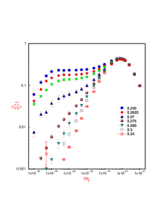
Figure 4: Semi-quenched condensate versus the valence quark mass $m_{\zeta}$ for two-flavor QCD [73] with a sea mass $m_{s}a=0.01$ (left). The result on the right is from a chiral random matrix model. See text.

4.1.6 Finite Chemical Potential

The case of finite chemical potential can be analyzed in a similar way, using instead

$$\left(\begin{array}[]{cc}0&i\mu\\ i\mu&0\end{array}\right)+\left(\begin{array}[]{cc}0&W^{\dagger}\\ W&0\end{array}\right)\,.$$ (109)

The deterministic part is now nonhermitian and we have two distinct regions (at least in the quenched case) on the complex plane. The Green’s function in the holomorphic region outside the blob of eigenvalues is given by (105) with the substitution $\pi^{2}T^{2}\longrightarrow-\mu^{2}$:

$$G^{3}-2zG^{2}+(z^{2}+\mu^{2}+1)G-z=0\,.$$ (110)

In order to find the boundary of the nonholomorphic region we may exploit the method of conformal mapping via the Blue’s functions, and transform the cuts of the $T\neq 0$ case into the boundary (see Fig. 5) by the transformation

$$z\longrightarrow iw=z-2G(z)$$ (111)

where $G(z)$ is the appropriate branch of the cubic equation (105) with the formal identification $\pi^{2}T^{2}=+\mu^{2}$. The extra factor of $i$ corresponds to the rotated Hamiltonian (here the deterministic as opposed to the random part is antihermitian).

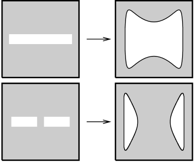
Figure 5: Conformal mapping from temperature to chemical potential. The one- and two-arc cuts (left) are mapped onto islands (right). The shaded region is the holomorphic support of the mapping.

The result of this mapping is in total agreement with a result derived originally by Stephanov [75] using a variant of the replica technique for the identical problem. The domains encircled by the mapping (111) defines the support of the complex eigenvalues of (109). In this region the resolvent $G(z)$ is non-analytic. The analytical resolvent following from (110) defines the correct branch in the holomorphic (shaded region), but fails on the boundary where the $1/N$ expansion breaks down. The failure is caused by the accumulation of eigenvalues in the plane, and signals large fluctuations in the phase of (109) as well as its correlations [76]. Similar effects are observed in quenched lattice calculations [77].

This effect is an artifact of the quenching (suppression of the fermion determinant) in the calculation of the resolvent which is a singular operator [18]. This may be overcome by unquenching at the price of much larger precision in the numerics, due to the presence of phase oscillations [78], or analyzing non-singular operators such as the partition function, which are self-quenched in the large $N$ limit [18, 31, 34]. High precision calculations for the unquenched partition function $Z_{N}(z=0,m)$ with $N_{f}=1$ are shown in Fig. 6 (dotted line). The solid lines refer to the two holomorphic solutions of (110). The long arrows indicate the points where the islands of non-analyticity in the quenched resolvent cross the real axis. The short arrow is the position of the cusp resulting from the intersection of the two holomorphic solutions to (110).

Figure 6: Unquenched free energy for $N_{f}=1$ at $\mu^{2}=0.8$ (left) and $\mu^{2}=1.2$ (right). The dots are high precision numerical results, while the solid lines follow from the solutions to (110). See text.

The phase structure of (109) directly follows from the analytical properties of the partition function $Z_{N}(z,\mu)$ for general complex $z=im$ with $N_{f}\neq 0$ and in the $1/N$ approximation as also noticed in [75]. In our case, this can be readily done using the integration law for Blue’s functions and the holomorphic solutions to (110) [18]. The outcome is simple: $Z_{N}$ develops cusps in the $z$- or $\mu$-plane that reflect on the two-branches of (110), with end-points conditioned by $B^{\prime}(G)=0$, in agreement with the results in [75]. The curves of zeroes obtained in this way are also in agreement with the (high-precision) numerics of [79]. The location of all zeroes follow from the analytical condition (43), here

$${\rm Re}\left[G^{2}_{i}(z)-G^{2}_{j}(z)+\log\frac{z-G_{i}(z)}{z-G_{j}(z)}+\log\frac{G_{j}(z)}{G_{i}(z)}\right]=0$$ (112)

where the labels $i,j$ refer to the different branches of the solutions (110). The density of zeroes follows accordingly from (47).

Using similar techniques one could also calculate the effect of fluctuations ($1/N$ corrections to the one-point Green’s function), with the result [18]

$$Z_{N}(z,\mu)=e^{NE_{0}}\cdot\left(\left\{D^{-2}[(D^{2}+\mu^{2})^{2}-(z-G)^{4}]\right\}^{-\frac{1}{2}}+{\cal O}\left(\frac{1}{N}\right)\right)\,.$$ (113)

Both $E_{0}$ and $D$ depends functionally on $G$ to this order. Hence, the information carried by the Blue’s functions condition the analytical behavior of (113). In particular, the location of the zeros of the curly bracket coincide with the points at which the $1/N$ expansion breaks down. These are exceptional points that may signal the onset of new scaling regimes for a new class of microscopic universalities in the context of non-hermitian random matrix models [18, 80].

Figure 7: Sample distribution of eigenvalues for different $\mu^{2}$. The solid lines follow from the conformal mapping.

4.1.7 Phase-Diagram

For general finite $T$ and finite $\mu$ the discussion about the thermodynamics of chiral random matrix models is very much model dependent, much like the thermodynamics in the Nambu-Jona-Lasinio model or the instanton liquid model. It is simply that of ‘constituent quarks’, with one quark and one anti-quark state (two-level) [31, 34]. In the absence of matter, chiral symmetry is spontaneously broken by filling the ‘negative-energy’ state. In the presence of matter, the symmetry is restored by depleting the ‘negative-energy’ state and filling the ‘positive-energy’ state with equal weight (finite T), or when the quark chemical potential reaches the ‘positive-energy’ state (finite $\mu$). In the first case the transition is second order, while in the first case it is first order. Diquarks effects in the present chiral random matrix models are down by $1/N$, and hence they decouple in the large $N$ limit. They are inessential for the thermodynamics in these models. Although unwelcome for $N_{c}\geq 3$ QCD because of color confinement (zero triality), they are dominant for $N_{c}=2$ QCD where they play the role massless baryons. 

Having said this, we now consider (96) with infinitely many Matsubara modes. This is essential when departing from the critical points, or in taking the temperature to zero for fixed $\mu$ [31]. In the chiral limit, the quark condensate $|\langle\overline{q}q\rangle|=P_{*}$ (spectral density $\nu(0)$), follows from the saddle point equation to the partition function associated to (96), that is [31, 34]

$$2\Sigma P_{*}=1-\frac{1}{1+e^{(|P_{*}+m|-\mu)/T}}-\frac{1}{1+e^{(|P_{*}+m|+\mu)/T}}\,.$$ (114)

The solution to (114) for $m=0$ is shown in Fig. 8. For $\mu>1/6\Sigma\ln{(2+\sqrt{3})}$, the transition is first order and disappears at $\mu_{*}=1/2\Sigma$. At $\mu=0$, the transition is second order (mean-field) and sets in at $T_{*}=1/4\Sigma$. The mismatch with the $T_{*}=1/\pi$ quoted in section 3.1.6 is due to: a different normalization for $\Sigma$ and an infinite number of Matsubara modes. The behavior shown in Fig. 8 is overall consistent with results in four dimensions using constituent quark models, $e.g.$ [35]. We refer to [31, 34] for further details on some of these and other issues in relation to phase changes. We note that the result for $\mu=0$ was also reproduced by [81] using a similar random matrix model. The effects of the inclusion of more Matsubara modes was also investigated in [82].

Figure 8: $|\langle\bar{q}q\rangle|$ from (114) with $\Sigma=1/4$ and $m=0$.

4.2 Strongly Nonhermitian Ensembles

The theory of open quantum systems plays a key role in many areas of physics and chemistry [83]. Microscopic treatment of dissipative evolution involves hermitian Hamiltonians. However, the use of non-hermitian Hamiltonians has been found to provide a convenient way to give a reduced description of the system. In this case, the hermitian part of the Hamiltonian refers to the free undamped dynamics whereas the nonhermitian remainder describes the damping imposed on the system by some external source. In this section, we will show a few applications of the Blue’s functions for dissipative systems, where the effective Hamiltonian is obtained by the standard Wigner-Weisskopf [84] reduction by partition. Reduction by partition follows from dividing the whole Hilbert space into two subspaces, and then the Hamiltonian is integrated over one of them. In this way one reduces the eigenvalue problem of high dimension to a lower one, and the resulting nonhermicity of the effective Hamiltonian comes from the “leakage of probability” due to the truncated vectors of the original Hilbert space.

4.2.1 Open Chaotic Scattering

We start from non hermitian random matrix model introduced by Mahaux and Weidenmüller [85] for resonance scattering. In brief, a quantum system composed of $(N-M)$ closed and $M$ open channels can be described by the effective scattering Hamiltonian

$$H=H_{R}+H_{\Gamma}\equiv H_{R}-ig\Gamma\qquad,\qquad\Gamma=AA^{T}$$ (115)

which is $N\!\times\!N$ dimensional. $A$ is an asymmetric $N\!\times\!M$ random matrix, $H_{R}$ is random Gaussian Hamiltonian and $g$ an overall coupling. Unitarity enforces the form of $\Gamma$ used in (115). The matrix elements $A_{k}^{a}$ characterize the transition between the $(N-M)$-internal channels and $M$-external channels, and are assumed to be independent of the scattering energy. For $M=0$, the Hamiltonian is real and the spectrum is bound. For $M\neq 0$, the Hamiltonian is complex, with all states acquiring a width. In what follows, we will solve the system by “decomposition” into subsystems and consecutively apply the methods presented above for Blue’s functions.

First consider the case of an $N\!\times\!N$ real symmetric product matrix $\Gamma^{S}_{kl}=A^{a}_{k}A^{a}_{l}$. Note that the Green’s function (for even random potentials) for the square of a square matrix is related to the Green’s function for the unsquared one via $G(z^{2}=w)=G(z)/z$, due to the identity

$$G(w)=\left<{\rm Tr}\frac{1}{w-A^{2}}\right>=\frac{1}{2z}\left<{\rm Tr}\frac{1}{z-A}\right>+\frac{1}{2z}\left<{\rm Tr}\frac{1}{z+A}\right>\,.$$ (116)

From (116) and (3), we infer the resolvent for the square of the Gaussian

$$G_{\!A^{\!2}}=\frac{1}{2}\left(1-\sqrt{1-\frac{4}{z}}\right)\,.$$ (117)

Second, let us observe, that the case of rectangular $N\times M$ matrices with $N,M\rightarrow\infty$ but $m=M/N$ fixed, follows by truncation using the projector [86]

$$P={\rm diag}(\underbrace{1,\ldots,1}_{M},\underbrace{0,\dots,0}_{N-M})$$ (118)

that is $\Gamma=\Gamma^{S}P$. We recognize the problem of “multiplication” of the random matrix $\Gamma^{S}$ by the deterministic projector P, and therefore could use the multiplication law for the Blue’s functions, hence the S-transform. The construction of the resolvent for the projector is straightforward

$$G_{P}(z)\equiv\frac{1}{N}{\rm Tr}\frac{1}{z-P}=m\frac{1}{z-1}+(1-m)\frac{1}{z}\,.$$ (119)

Using the relations for “multiplication law” from the previous part we obtain the S-transform

$$S_{P}(z)=\frac{1+z}{m+z}\ .$$ (120)

Similarly, the S-transform for the Green’s function for the square of the Gaussian (117) is

$$S_{\!A^{\!2}}=\frac{1}{1+z}\ .$$ (121)

The product reads

$$S=S_{\!A^{\!2}}\cdot S_{P}=\frac{1}{m+z}$$ (122)

so inverting the order of reasoning we get for the resolvent

$$G(z)=\frac{1-m}{2z}+\frac{1}{2}\left[1\pm\sqrt{\left(\frac{1-m}{z}-1\right)^{2}-\frac{4m}{z}}\right]\,.$$ (123)

Note that the $1/z$ terms (first term and a term under the square root) represent $(N-M)$ zero modes of the matrix $\Gamma$.

Now we could “add” the Hamiltonians $H_{R}$ and $-ig\Gamma$, by constructing the generalized Blue’s functions. Let us first write down the hermitian Blue’s functions for $H_{R}$ and $g\Gamma$. The first Blue’s function, coming from inverting (3) is

$$B_{1}(z)=z+\frac{1}{z}\,.$$ (124)

The second one is the functional inverse of (123), therefore

$$B_{2}(z)=\frac{mg}{1-gz}+\frac{1}{z}\,.$$ (125)

Then the generalized Blue’s functions read

$${\cal B}_{1}({\cal Z}) = {\cal Z}+\frac{1}{{\cal Z}}$$

$${\cal B}_{2}({\cal Z}) = m(1-\hat{g}{\cal Z})^{-1}\hat{g}+\frac{1}{{\cal Z}}$$ (126)

where the coupling $\hat{g}$ is a matrix $\hat{g}={\rm diag}(-ig,ig)$. The signs in the matrix coupling reflects the fact, that the complex conjugate “copy” interacts with opposite coupling constant. Then, the generalized addition law for the Blue’s functions leads to the final matrix equation for the Green’s function

$${\cal Z}=m(1-\hat{g}{\cal G})^{-1}\hat{g}+{\cal G}+\frac{1}{{\cal G}}\,.$$ (127)

Nontrivial (nonholomorphic) solution to the matrix equation (127) provides full information on the eigenvalue distribution. The condition $G_{q\bar{q}}=0$ defines the boundaries of the eigenvalue distribution, and the divergence of $G_{qq}$ (Gauss law) gives the desired spectral density of eigenvalues on the islands. Instead of presenting the explicit formulae, we show the figures with few sample solutions (figure 9).

Figure 9: Comparison of the numerically generated distribution of eigenvalues for few sample couplings in the model (115) with the analytical results. The solid lines represent the boundaries following from the condition $G_{q\bar{q}}=0$.

The results obtained above were obtained also by other methods [87], so we do not need to dwell on their physical content. However, we encourage the reader to compare the present derivation with the derivations of the same result based on the replica or supersymmetric methods (see e.g. [88, 89]).

4.2.2 Bridging via Dissipation

We conclude this brief overview by another example, where analytical results were obtained by direct application of the generalized Blue’s functions. This is the model of an effective two-level system, coupled to a noise reservoir of the random type [90]. Such systems could e.g. serve as model systems for electron or proton transfers in condensed phase reactions in the field of chemical physics. The deterministic part of the Hamiltonian is given by an effective two-level system with N electrons, building up two close energy states with half of the energies equal to $\epsilon$ and other half equal to $-\epsilon$. For the dissipative part, we take $H_{\Gamma}$ from (115), therefore the effective Hamiltonian reads

$$H=H_{D}-igAA^{\dagger}\,.$$ (128)

The deterministic Green’s function for two levels is

$$G_{D}=\frac{1}{2}(\frac{1}{z-\epsilon}+\frac{1}{z+\epsilon})$$ (129)

therefore the relevant generalized Blue’s function is given by the matrix equation

$${\cal Z}=\frac{1}{2}\left[({\cal B}_{D}({\cal Z})-\epsilon)^{-1}+({\cal B}_{D}({\cal Z})+\epsilon)^{-1}\right]\,.$$ (130)

The generalized Blue’s function for the noise term is just ${\cal B}_{2}$ in (126). The generalized addition law for the Blue’s functions leads at once [90]

$${\cal G}=\frac{1}{2}\left[({\cal Z}-m(1-\hat{g}{\cal G})^{-1}\hat{g}-\epsilon)^{-1}+({\cal Z}-m(1-\hat{g}{\cal G})^{-1}\hat{g}+\epsilon)^{-1}\right]\,.$$ (131)

As in the previous example, one easily infers the spectral density of the system (128) from the nonholomorphic solution to the equation. Again, we present a figure instead of the explicit formulae (see figure 10).

Figure 10: Comparison of the numerically generated distribution of eigenvalues for few sample parameters of the model (128). The solid lines represent the boundaries following from the analytical condition $G_{q\bar{q}}=0$.

We would like to note two “phase transitions” visible easily from the change of character of the envelopes. Here the envelope is represented by the solid curve, obeying the analytical solution to $G_{q\bar{q}}=0$, here given by the 8th order polynomial in $x$ and $y$ ( with $z=x+iy$). The first phase transition (figure 10(left)$\rightarrow$ 10(middle)) corresponds to the emergence of the noise-induced “bridging states”. The second phase transition, present at large coupling constant (figure 10(middle) $\rightarrow$ 10(right)) corresponds to the “collectivization of the spectra”[91]. The upper island represents direct resonances, the lower island represents the (long-lived) coherent state, caused by the explicit presence of zero modes in the dissipative part of the Hamiltonian.

4.3 Weakly Nonhermitian Ensembles

As a final application of the Blue’s function techniques we will consider the model of Hatano and Nelson [92] (HN) for nonhermitian localization, which has recently attracted much attention [8, 93, 94]. This model is a non-hermitian version of the Anderson model, hence quantum mechanical in nature. Nevertheless, the method of Blue’s functions will turn out to be very appropriate for its treatment, since it is equivalent to the Coherent Phase Approximation (CPA) widely used in the treatment of hermitian models with site disorder [95].

In their original analysis, Hatano and Nelson [92] have shown that the depinning of the flux lines from columnar defects in superconductors in $d+1$-dimensions may be mapped onto the world-lines of bosons on a $d$-dimensional hyperlattice. The localization by defects was approximated by an on-site randomness on the hyperlattice, and the depinning induced by the transverse magnetic field was found to cause a directed hopping of the bosons on the hyperlattice, resulting in a nonhermitian quantum Hamiltonian.

Figure 11: Eigenvalue distribution in the Hatano-Nelson model for large (left), intermediate (middle) and small (right) $h$. The two dots refer to the location of the forking (A) and the maximal imaginary eigenvalue (B).

The HN model (for $d=1$) is given by the following Hamiltonian

$$H=H_{0}+V_{A}=\sum_{A=1}^{N}\frac{t}{2}\left(e^{h}c^{\dagger}_{A+1}c_{A}+e^{-h}c^{\dagger}_{A-1}c_{A}\right)+V_{A}c^{\dagger}_{A}c_{A}$$ (132)

where the $c^{\dagger}_{A}$ is a boson creation operator at site $A$. The lattice spacing is set to 1. The hopping strength is $te^{\pm h}$, where $h$ is the strength of the “transverse magnetic field” [92] in units of the flux quantum. Diagonal randomness is represented by random variables $V_{A}$, originally taken from a uniform distribution in the interval $[-\Delta,\Delta]$. For $h\neq 0$, the eigenvalues are complex. As stated earlier, this is a nonhermitian analogue of the Anderson model in $d=1$ dimension. The eigenstates of this Hamiltonian with an eigenvalue $\lambda$ such that ${\rm Im}\lambda\neq 0$ are delocalized. For sufficiently large $h>h_{c}^{(2)}$ all states are delocalized and form a closed curve that looks like a deformed ellipse (see figure 11(left)). When $h$ is reduced below $h_{c}^{(2)}$, the eigenvalues at the edges snap to the real axis and get localized (see figure 11(middle)). Reducing $h$ further below $h_{c}^{(1)}$ causes the eigenvalues to fill in the whole interval on the real axis (see figure 11(right)). Our aim here is to understand these effects quantitatively, using the method of Blue’s functions.

The relevant quantity to calculate is the Green’s function

$$G(z)=\frac{1}{N}\left<{\mbox{\rm tr}\,\frac{1}{z-H}}\right>\,.$$ (133)

Its holomorphic part is related to the derivative of $\det(z-H)$ outside (large $z$). A close look at (132) shows that before averaging over $V_{A}$,

$$\det(z-H)\sim\left(\frac{t}{2}\right)^{N}\cdot\left[e^{Nh}+e^{-Nh}\right]+f(z,N,V_{A})$$ (134)

where the function $f$ does not depend on $h$ and has the leading order behavior

$$f(z,N)=e^{Nf_{out}(z,V_{A})}\cdot(1+{\rm corrections})$$ (135)

where the corrections are polynomial. For large $N$ there are two regimes: $h+\log(t/2)>f_{out}$ or $<f_{out}$. In the first regime the determinant is $z$-independent, hence $G(z)=0$, and we are inside the curves shown in 11(left),(middle). In the second regime the determinant is $h$-independent, hence $G(z)$ is also $h$-independent, and we are outside the curves.

Once we have $f_{out}$ we may calculate the critical parameters $h_{c}^{(1,2)}$, for which we have full characterization of the eigenvalue spectra. Note that $f_{out}$ depends explicitly on $V_{A}$. It may happen that for certain configurations of site randomness $V_{A}$ the $f$ term wins while for others the ‘$h$’ term dominates. This leads to a broadening of the curve of eigenvalues. This effect is difficult to control analytically, however numerical simulations suggest that this broadening is of order $1/\sqrt{N}$ [8]. This behavior is reminiscent of the case of weak nonhermiticity discussed recently in [96].

4.3.1 Coherent Phase Approximation

A direct calculation of $G(z)$ is involved. If we were to make a diagrammatic expansion we would find that a lot of nonplanar graphs would contribute. Furthermore one cannot do a perturbative expansion around $h$ small or big, neglecting the ‘hopping parameters’ above or below the diagonal of the Hamiltonian. This is not surprising, the HN model is just the nonhermitian version of the Anderson model in d-dimensions, for which there is no exact solution in large $N$ except for the special case of Cauchy randomness (Lloyd model) [97].

We have shown in [8] that by assuming the site randomness and the ‘hopping’ part of the Hamiltonian to be free, we can just apply the method of Blue’s functions to the present problem. In this approximation, we resum at once the planar diagrams and all non-planar diagrams with single-site rescattering (some sort of a mean-field analysis). This approximation bears much in common with the CPA method as we now show. Specifically, let

$$H=H_{D}+H_{R}$$ (136)

where $H_{D}$ is the deterministic hopping term and $H_{R}$ is the diagonal random matrix with random entries $V_{A}$. Let $G_{D}$ denote the deterministic Green’s function:

$$G_{D}(z)={\rm tr}\,\frac{1}{z-H_{D}}\,.$$ (137)

In the CPA the Green’s function of the system is given by

$$G(z)=G_{D}(z-\Sigma)$$ (138)

where $\Sigma$ satisfies the condition of [98]

$$\left<{\frac{V_{A}-\Sigma}{1-(V_{A}-\Sigma)G(z)}}\right>=0\,.$$ (139)

Multiplying by $G(z)$ and adding and subtracting 1 in the numerator we get

$$\left<{\frac{1}{1-(V_{A}-\Sigma)G(z)}}\right>=1$$ (140)

then multiplying by $G(z)$ once again, we obtain

$$G(z)=G_{R}\left(\frac{1}{G}+\Sigma\right)\,.$$ (141)

As a final step let us evaluate the Blue’s function for the random part $B_{R}$ on both sides of this equation

$$B_{R}(G(z))=\frac{1}{G(z)}+\Sigma\,.$$ (142)

But this is a direct consequence of the addition formula for Blue’s functions

$$B(z)=B_{R}(z)+B_{D}(z)-\frac{1}{z}\,.$$ (143)

Namely after reexpressing $B_{R}$ in terms of $B$ and $B_{D}$ we obtain

$$z-B_{D}(G(z))+\frac{1}{G(z)}=\frac{1}{G(z)}+\Sigma\,.$$ (144)

But now we may use the definition of $\Sigma$ (138) and get

$$z-B_{D}(G_{D}(z-\Sigma))=\Sigma$$ (145)

which finishes the proof.

We note that the above arguments do not rely on whether the starting Hamiltonian is hermitian or not. In the hermitian case our conclusion is in agreement with the one of Neu and Speicher [11], who used different arguments. Since the Green’s functions for the nonhermitian and hermitian ensembles coincide in the “outer” region, the addition of the Blue’s functions together with the balance of the free energies as detailed in the preceding sections, provide for a concise approximation scheme for nonhermitian localization in the large $N$ limit. We now proceed to implement this.

4.3.2 Nonhermitian Localization

The Green’s function for the deterministic part is just

$$G_{D}(z)=\frac{1}{N}\sum_{n=1}^{N}\frac{1}{z-t\cos(2\pi n/N+ih)}=\left\{\begin{array}[]{cl}1/\sqrt{z^{2}-t^{2}}&\mbox{``outside''}\\ 0&\mbox{``inside''}\end{array}\right.$$ (146)

where the last equality holds in the large $N$ limit. This shows that we may define the Blue’s functions only outside the curve of eigenvalues. There it is given by

$$B_{D}(z)=\sqrt{\frac{1}{z^{2}}+t^{2}}\,.$$ (147)

The Blue’s function for the site randomness $V_{A}$ is fixed by the type of distribution we select. For the (solvable) case of a semicircular distribution, the Blue’s function is

$$B_{R}^{semicircular}(z)=z+\frac{1}{z}$$ (148)

while for a uniform distribution of width $\Delta$ it is

$$B_{R}^{uniform}(z)=\Delta\coth\Delta z$$ (149)

and for a Cauchy distribution

$$B_{R}^{Cauchy}(z)=\frac{1}{z}-i\gamma\,.$$ (150)

Therefore the Blue’s function for the HN Hamiltonian is

$$B(z)=B_{D}(z)+B_{R}(z)-\frac{1}{z}\,.$$ (151)

So the Green’s function (in CPA) would satisfy the equation $B(G(z))=z$. In particular, for a uniform distribution the Green’s function satisfies

$$z=\sqrt{\frac{1}{G^{2}}+t^{2}}+\Delta{\rm coth}\Delta G-1/G$$ (152)

while for a Cauchy distribution it satisfies

$$\sqrt{\frac{1}{G^{2}}+t^{2}}-i\gamma=z\,.$$ (153)

Integrating the Blue’s function for the HN Hamiltonian gives the free energy $f_{out}$ (in this case a direct integration of $G$ would be infeasible)

$$f_{out}(z)=\Delta G\coth\Delta G-1+\log\frac{1+\sqrt{1+G^{2}}}{2}-\log\frac{\sinh\Delta G}{\Delta}$$ (154)

for uniform randomness and

$$f_{out}(z)=\log(i\gamma+z+\sqrt{(i\gamma+z)^{2}-t^{2}})-\log 2$$ (155)

for Cauchy randomness.

We will now calculate $h_{c}^{(1)}$ — the value of $h$ where the curve of eigenvalues starts to appear (i.e. when point B in figure 11 leaves the origin along the imaginary axis). This is determined by the condition that the boundary between the two phases passes through $z=0$

$$h+\log\frac{t}{2}=f_{out}(0)\,.$$ (156)

For a uniform distribution (154) the solution of the analytical condition (156) is only possible numerically. In figure 12 we compare this solution to the exact numerical values for the HN Hamiltonian. The agreement is fairly good. For a Cauchy distribution, the critical condition (156) is simply

$$\sinh h_{c}^{(1)}=\frac{\gamma}{t}\,.$$ (157)

The same condition was obtained by Brézin and Zee [94], and Goldsheid and Khoruzenko [93], using different arguments. We note, in agreement with these authors, that in the case of Cauchy randomness the results are exact, much like the Lloyd model in the hermitian case.

Figure 12: Dependence of A (forking point) and B (top point on the imaginary axis upon lift-off at $z=0$) versus $h$ for $\Delta=1$ (uniform randomness). The solid lines follow from the analytical results using the addition law (CPA).

5 CONCLUSIONS

Voiculescu’s free random variable approach has a simple realization in terms of Blue’s functions, as originally suggested by Zee[9]. This applies for both the R- and S-transforms. In the first part of these lectures, we have gone over the essentials of Blue’s function calculus, emphasizing the generic aspects which are important in physical settings. The addition and multiplication of free random Hamiltonians translates simply to the addition and multiplication of the pertinent Blue’s functions. More importantly, their extrema are in one-to-one correspondence with the end-points of pertinent eigenvalue distributions, and their analytical structure conditions the singularity structure of appropriate partition functions. Moreover Blue’s functions provide a surprising method of finding the boundary of the support of eigenvalues for nonhermitian ensembles through conformal mappings.

The free random treatment of matrix models amenable to a $1/N$ expansion is usually exact to leading order in $1/N$, hence in agreement with the treatment based on more conventional methods. The advantage of the former being its simplicity. For disordered models which are not immediately amenable to a $1/N$ expansion, the free random treatment provides for an approximation that is identical to the CPA approximation. The latter has been successfully applied to the Anderson model [1], and its variants [11, 12]. The free random variable approach goes beyond Gaussian measures, and applies equally well to random matrix models as well as quantum models with diagonal disorder [8].

In the second part of these lectures we have discussed effective QCD in light of the spontaneous breaking of chiral symmetry in the vacuum. Using power counting both in the microscopic and macroscopic limit, we have argued that the partition function in the large volume limit is solely conditioned by the mode of symmetry breaking on the pertinent coset span by the little group [37, 40]. The stability of the partition function against soft and hard quantum corrections, conditions the universal behavior of the spectral oscillation of the QCD Dirac operator both at zero virtuality and in the bulk of the infrared region. For chiral random matrix models this means simply that arbitrary polynomial weights that are chirally invariant yield by power counting the same universal spectral oscillations in the vacuum.

The universal behavior of spectral oscillations in effective QCD occurs in the microscopic limit with light quark masses (for chiral symmetry to be relevant) and large enough volumes (for nonperturbative physics to set in). This is the limit, however, where the vacuum has no spontaneous alignment yet (the chiral condensate is driven by the light quark masses). The universality arguments do not carry any dynamical content. Rather, they reflect on the kinematical correlations induced by the compactness of the coset space associated to the would-be Goldstone modes, in the presence of a universal $(N_{f},N_{f})$ symmetry breaking pattern.

When these arguments are combined with the universality of the chiral phase transition as advanced by Pisarski and Wilczek [51] in the context of QCD, they show that these oscillations survive the effects of matter at the critical point, thereby generalizing the arguments in the vacuum. Although our arguments were restricted to effective QCD, they apply equally well to QCD in odd dimensions, as well as effective fermionic theories with spontaneous symmetry breaking such as the Nambu-Jona-Lasinio models or the instanton models. For the latter spectra, we note that power counting is simplified on the hypertorus. These assertions can be readily checked.

In the third part of these lectures, we have applied some of the Blue’s function techniques to chiral random matrix models, in the non-universal regions where the $1/N$ expansion applies. The latters belong to a cohort of effective models of QCD in the long wavelength limit, that reproduce the microscopic sum rules. In the macroscopic limit they are consistent with power counting only at tree level, hence their limited range of consistency with the QCD Ward identities. They are however useful for addressing issues related to the thermodynamical limit, as well as mean-field regions in most of the phase transitions, barring the case of large Ginzburg windows [100]. In their standard form they are schematic versions of the instanton model to the QCD vacuum. Unlike the latter, however, they can be extended to accommodate microscopic QCD in odd dimensional spaces where the issue of chiral symmetry is subtle, and the question of instantons obsolete.

As effective models of QCD in the infrared, the chiral random matrix models can be used to illustrate the subtleties between the large volume limit versus the smallness or largeness of the QCD external parameters. In this respect, we have analyzed the U(1) problem, and the dependence of the vacuum partition function on the $\theta$ angle. In both cases the large volume limit is subtle when light quarks are present. Needless to say, that lattice QCD simulations at finite $\theta$ are not yet available, owing to the complex character of the fermion determinant.

We have shown that the concept of addition law of Blue’s functions finds a simple realization when the temperature or quark chemical potential are schematically inserted in the standard chiral random matrix models. These models are tied to QCD only in the context of mean-field universality, and may be given non-standard versions to accommodate for non-mean-field universalities. As effective models to the QCD phase transition, they can be regarded as crude variants of the Nambu-Jona-Lasinio model, or the instanton model, to which they naturally relate. We stress, however, their simplicity and also their user-easy access to the quark spectra. Under a phase change, the latters are expected to undergo structural changes near zero virtuality provided that the soft and hard modes decouple in the large volume limit. This is the case for infrared sensitive observables, including order parameters. In this sense, our comparison to the present lattice data at the transition point is striking [74]. We note, however, that the absence of thermal and Fermi motion in these models, makes their extension to most observables suggestive at best.

Chiral random matrix models of effective QCD are also interesting because they tie some of the fundamental aspects of QCD to other models of disorder. In this context chiral random matrix models at finite chemical potential resemble closely models of disorder with dissipation. The analysis in terms of Blue’s functions generalize handily to these cases as well.

We have presented models with strong dissipation, currently in use to model quantum chaotic scattering with many open channels, as well as models of weak dissipation, such as the model recently discussed by Hatano and Nelson. The latter is disordered quantum mechanics in $d$ dimensions, that is still amenable to random matrix techniques provided that freeness is used. We have shown that this approximation is identical to the CPA approximation commonly in use for hermitian disordered problems (e.g. Anderson model).

The models of strong nonhermiticity discussed here, apply to a large number of physical phenomena. They show up in nuclear, atomic and molecular spectroscopy, mesoscopic ballistic devices, microwave cavities and the physics of condensed state chemical reactions, to cite a few [88]. Our method should shed more light on the already existing analyses.

The current models of weak nonhermiticity offer new field of investigations that are worth pursuing with the present methods. The model of Hatano and Nelson [92] (nonhermitian analogue of the Anderson model [1]) for the description of flux depinning in type II superconductors offers a good starting point. It is a canonical example of nonhermitian localization, that may become relevant to a variety of other models with a directed diffusion, such as: models for the growth of bacterial populations [101], models for spreading genetic mutations, models of chemical reactions, neural networks, turbulence, and models of growth of monetary capital. We are confident that Voiculescu’s idea of freeness will open a vested interest in this rich array of problems.

6 Acknowledgments

This work was partially supported by the US DOE grant DE-FG-88ER40388, by the Polish Government Project (KBN) grants 2P03B19609 and 2P03B04412 and by Hungarian grants OTKA T022931 and FKFP0126/1997.

REFERENCES

- [1] P.W. Anderson, Phys. Rev. 109, 1492 (1958).
- [2] O. Bohigas and M. Giannoni, Lecture notes in Physics 209, Ed. Springer Verlag 1984.
- [3] E.P. Wigner, Proc. Camb. Phil. Soc. 47, 790 (1951).
- [4] C.E. Porter, “Statistical Theory of Spectra: Fluctuations” , Academic Press, New York (1965).
- [5] F.J. Dyson, J. Math. Phys. 13, 90 (1972).
- [6] M.L. Mehta, “Random Matrices” , Academic Press, New York (1991).
- [7] D.V. Voiculescu, Invent. Math. 104, 201 (1991); D.V. Voiculescu, K.J. Dykema and A. Nica, “Free Random Variables” , Am. Math. Soc., Providence, RI, (1992); for new results see also A. Nica and R. Speicher, Amer. J. Math. 118, 799 (1996) and references therein.
- [8] R.A. Janik, M.A. Nowak, G. Papp and I. Zahed, e-print cond-mat/9705098.
- [9] A. Zee, Nucl. Phys. B474, 726 (1996).
- [10] R. Speicher, Math. Ann. 298, 611 (1994).
- [11] P. Neu and R. Speicher, Jour. Stat. Phys. 80, 1279 (1995).
- [12] F. Wegner, Phys. Rev. B19, 783 (1979).
- [13] For a recent review, see T. Guhr, A. Müller-Gröling and H.A. Weidenmüller, e-print cond-mat/9707301.
- [14] P. Di Francesco, P. Ginsparg and J. Zinn-Justin, Phys. Rept. 254, 1 (1995), and references therein.
- [15] see e.g. E. Brézin and A. Zee, Phys. Rev. E49, 2588 (1994); E. Brézin and A. Zee, Nucl. Phys. B453, 531 (1995); E. Brézin, S. Hikami and A. Zee, Phys. Rev. E51, 5442 (1995).
- [16] H.-J. Sommers, A. Crisanti, H. Sompolinsky and Y. Stein, Phys. Rev. Lett. 60, 1895 (1988).
- [17] B. Derrida, L. De Seze and C. Itzykson, J. Stat. Phys. 33, 559 (1983).
- [18] R.A. Janik, M.A. Nowak, G. Papp and I. Zahed, Nucl. Phys. B501, 603 (1997).
- [19] J. Feinberg and A. Zee, e-print cond-mat/9703087.
- [20] R.A. Janik, M.A. Nowak, G. Papp, J. Wambach and I. Zahed, Phys. Rev. E55, 4100 (1997).
- [21] J. Feinberg and A. Zee, e-print cond-mat/9704191.
- [22] R.A. Janik, Ph.D. Thesis, Cracow 1997 (unpublished).
- [23] K. Huang, “Statistical Mechanics” , John Wiley, New York, (1987).
- [24] J. Vink, Nucl. Phys. B323, 399 (1989).
- [25] R. Shrock, private communication; G. Marchesini and R. Shrock, Nucl. Phys. B318, 541 (1989); V. Matveev and R. Shrock, J. Phys. A28, 1557 (1995); Nucl. Phys. Proc. Suppl.B42 776 (1995).
- [26] J. Ambjørn, J. Jurkiewicz and Yu.M. Makeenko, Phys. Lett. B251, 517 (1990).
- [27] J. Ambjørn, C.F. Kristjansen and Yu.M. Makeenko, Mod. Phys. Lett. A7, 3187 (1992).
- [28] G. Akemann and J. Ambjørn, J. Phys. A29, L555 (1996); G. Akemann, Nucl. Phys. B482, 403 (1996); G. Akemann, e-print hep-th/9702005.
- [29] J. Ambjørn, L. Chekhov, C.F. Kristjansen and Yu. Makeenko, Nucl. Phys. B404, 127 (1993).
- [30] E. Brézin and A. Zee, Nucl. Phys. B402, 613 (1993).
- [31] R.A. Janik, M.A. Nowak and I. Zahed, Phys. Lett. B392, 155 (1997); R.A. Janik, M. A. Nowak, G. Papp and I. Zahed, Acta Phys. Pol. B27, 3271 (1996).
- [32] M.J. Bowick and E. Brézin, Phys. Lett. B268, 21 (1991).
- [33] J.J.M. Verbaarschot and I. Zahed, Phys. Rev. Lett. 70, 3852 (1993).
- [34] M. A. Nowak, M. Rho and I. Zahed, “Chiral Nuclear Dynamics” , World Scientific, Singapore, (1996).
- [35] for a review see U. Vogel and W. Weise, Prog. Part. and Nucl. Phys. 27, 195 (1991); S.P. Klevansky, Rev. Mod. Phys. 64, 649 (1992); M.K. Volkov, Phys. Part. Nucl. 24, 35 (1993); T. Hatsuda and T. Kunihiro, Phys. Rep. 247, 221 (1994).
- [36] for recent reviews, see T. Schäfer and E.V. Shuryak, e-print hep-ph/9610451; D. Diakonov, e-print hep-ph/9602375.
- [37] J. Gasser and H. Leutwyler, Ann. Phys. 158, 142 (1984).
- [38] H. Yamagishi and I. Zahed, Ann. Phys. 247, 292 (1996).
- [39] E. Witten, Ann. Phys. 128, 363 (1980).
- [40] H. Leutwyler and A. Smilga, Phys. Rev. D46, 5607 (1992).
- [41] M.A. Nowak, J.J.M. Verbaarschot and I. Zahed, Nucl. Phys. B325, 581 (1989).
- [42] E. Shuryak and J.J.M. Verbaarschot, Nucl. Phys. A563, 306 (1993).
- [43] T. Banks and A. Casher, Nucl. Phys. B169, 103 (1980).
- [44] R. Alkofer, M.A. Nowak, J.J.M. Verbaarschot and I. Zahed, Phys. Lett. B233, 205 (1989).
- [45] J.J.M. Verbaarschot, Phys. Rev. Lett. 72, 2531 (1994); J.J.M. Verbaarschot, Nucl. Phys. B426, 559 (1994).
- [46] S. Nishigaki, Phys. Lett. B387, 707 (1996); G. Akemann, P. Damgaard, U. Magnea and S. Nishigaki, Nucl. Phys. B487, 721 (1997).
- [47] M.A. Halasz and J.J.M. Verbaarschot, Phys. Rev. Lett. 74, 3920 (1995)
- [48] J. Jurkiewicz, M.A. Nowak and I. Zahed, Nucl. Phys. B478, 605 (1996)
- [49] D.J. Gross and E. Witten, Phys. Rev. D21, 446 (1980)
- [50] J.J.M. Verbaarschot and I. Zahed, Phys. Rev. Lett. 73, 2288 (1994).
- [51] R. Pisarski and F. Wilczek, Phys. Rev. D29, 338 (1984).
- [52] A. Kocic and J. Kogut, Phys. Rev. Lett. 74, 3109 (1995).
- [53] A.D. Jackson, M.K. Sener and J.J.M. Verbaarschot, Nucl. Phys. B479, 721 (1996).
- [54] Yu.A. Simonov, Phys. Rev. D43, 3531 (1991).
- [55] S. Higuchi, C. Itoi, S. M. Nishigaki and N. Sakai, Phys. Lett. B318, 63 (1993); S. Higuchi, C. Itoi, S. M. Nishigaki and N. Sakai, Nucl. Phys. B434, 283 (1995).
- [56] M.A. Nowak, J.J.M. Verbaarschot and I. Zahed, Phys. Lett. B228, 251 (1989).
- [57] R.A. Janik, M.A. Nowak, G. Papp and I. Zahed, Nucl. Phys. B498, 313 (1997).
- [58] J.B. Kogut, J.F. Lagae and D.K. Sinclair, e-print hep-lat/9709067.
- [59] E. Brézin, S. Hikami and A. Zee, Nucl. Phys. B464, 411 (1996).
- [60] N.P. Landsman and C.G. van Weert, Phys. Rep. 145, 141 (1987).
- [61] M. Atiyah and I. Singer, Ann. Math. 87, 484 (1968).
- [62] S. Samuel, Mod. Phys. Lett. A7, 2007 (1992); H. Kikuchi and J. Wudka, Phys. Lett. B284, 111 (1992); I. Zahed, Nucl. Phys. B 427, 561 (1994); E. Shuryak and J.J.M. Verbaarschot, Phys. Rev. D52, 295 (1995).
- [63] D.I. Diakonov, M.V. Polyakov and C. Weiss, Nucl. Phys. B461, 539 (1996).
- [64] G. Schierholtz, Nucl. Phys. A37, 203 (1994); J.C. Plefka and S. Samuel, e-print hep-lat/9704016
- [65] R.A. Janik, M.A.Nowak, G. Papp and I. Zahed, to be published ,
- [66] R. Alkofer and I. Zahed, Phys. Lett. B238, 149 (1990).
- [67] R.F. Dashen, Phys. Rev. D3, 1879 (1971) .
- [68] J. Nuyts, Phys. Rev. Lett. 26, 1604 (1971).
- [69] M. Creutz, Phys. Rev. D52, 2951 (1995).
- [70] A.D. Jackson and J.J.M Verbaarschot, Phys. Rev. D53, 7223 (1996).
- [71] M.A. Nowak, G. Papp and I. Zahed, Phys. Lett. B389, 137 (1996).
- [72] L.A. Pastur, Theor. Mat. Phys. (USSR) 10, 67 (1972); F. Wegner, Phys. Rev. B19, 783 (1979); P. Neu and R. Speicher, J. Phys. A28, L79 (1995); E. Brézin, S. Hikami and A. Zee, Phys. Rev. E51, 5442 (1995); A. D. Jackson and J.J.M. Verbaarschot, Phys. Rev. D53, 7223 (1996); T. Wettig, A. Schäfer and H.A. Weidenmüller, Phys. Lett. B367, 28 (1996); J. Jurkiewicz, M.A. Nowak and I. Zahed, Nucl. Phys. B478, 605 (1996); M. Engelhardt, Nucl. Phys. B481, 479 (1996).
- [73] S. Chandrasekharan, N. Christ, Nucl.Phys.Proc.Suppl. 47, 527 (1996).
- [74] M.A. Nowak, G. Papp and I. Zahed, Phys. Lett. B389, 341 (1996).
- [75] M. Stephanov, Phys. Rev. Lett. 76, 4472 (1996); M. Stephanov, Nucl. Phys. Proc. Suppl. 53, 469 (1997).
- [76] R.A. Janik, M.A. Nowak, G. Papp and I. Zahed, Phys. Rev. Lett. 77, 4876 (1996).
- [77] For a recent review on lattice at finite chemical potential, see I. Barbour et al., e-print hep-lat/9705042.
- [78] R.A. Janik, M.A. Nowak, G. Papp and I. Zahed, (unpublished) , .
- [79] A. Halasz, A.D. Jackson and J.J.M. Verbaarschot, Phys. Lett. B395, 293 (1997); A. Halasz, A.D. Jackson and J.J.M. Verbaarschot, e-print hep-lat/9703006.
- [80] R.A. Janik, M.A. Nowak, G. Papp and I. Zahed, e-print hep-ph/9708418.
- [81] T. Wettig, T. Gühr, A. Schäfer and H.A. Weidenmüller, Hirschegg Lectures (1997), hep-ph/9701387.
- [82] G. Papp, Heavy Ion Physics 5, 255 (1997).
- [83] U. Weiss, “Quantum Dissipative Systems” World Scientific, Singapore, (1993); R.K. Wangness and F. Bloch, Phys. Rev. 89, 728 (1953); A.G. Redfield, Adv. Magn. Reson. 1, 1 (1965).
- [84] E.P. Wigner and V.F. Weisskopf, Z. Phys. 63, 54 (1930).
- [85] C. Mahaux and H.A. Weidenmüller, “Shell Model Approach to Nuclear Reactions” , North Holland, Amsterdam (1969).
- [86] D. Voiculescu, Inv. Math. 104, 201 (1991).
- [87] F. Haake et al., Zeit. Phys. B88, 359 (1992); N. Lehmann, D. Saher, V.V. Sokolov and H.J. Sommers, Nucl. Phys. A582, 223 (1995).
- [88] Y. V. Fyodorov and H.-J. Sommers, J. Math. Phys. 38, 1918 (1997), and references therein.
- [89] K.B. Efetov, Adv. in Phys. 32, 53 (1983); J.J.M. Verbaarschot, H.A. Weidenmüller and M. R. Zirnbauer, Phys. Rep. 129, 367 (1985).
- [90] E. Gudowska-Nowak, G. Papp and J. Brickmann, Chem. Phys. 220, 125 (1997).
- [91] V.V. Sokolov and V.G. Zelevinsky, Nucl. Phys. A504, 562 (1989).
- [92] N. Hatano and D.R. Nelson, Phys. Rev. Lett. 77, 570 (1997); N. Hatano and D.R. Nelson, e-print cond-mat/9705290.
- [93] P.W. Brouwer; P.G. Silvestrov and C.W.J. Beenakker, e-print cond-mat/9705186; J.T. Chalker and Z. Jane Wang, Phys. Rev. Lett. 79, 1797 (1997); J. Feinberg and A.Zee, e-print cond-mat/9706218; I.Y. Goldsheid and B.A. Khoruzhenko, e-print cond-mat/9707230; see also [94].
- [94] E. Brézin and A. Zee, e-print cond-mat/9708029, and references therein.
- [95] I.M. Lifshitz, S.A. Gredeskul and L.A. Pastur, “Introduction to the Theory of Disordered Systems” , Wiley, New York (1988).
- [96] Y.V. Fyodorov, B.A. Khoruzhenko and H.-J. Sommers, Phys. Lett. A226, 46 (1997), and references therein; K. B. Efetov, Phys. Rev. Lett. 79, 491 (1997).
- [97] P. Lloyd, J. Phys. C2, 1717 (1969).
- [98] J.M. Ziman, “Models of Disorder” , Cambridge Univ. Press, New York (1979).
- [99] H. Maassen, J. Funct. Anal. 106, 409 (1992); H. Bercovici and D. Voiculescu, Indiana U. Math. J. 42, 733 (1993).
- [100] M. Plischke and B. Bergersen, “Equilibrium Statistical Physics” , Ed. Prentice Hall (1989).
- [101] D.R. Nelson and N.M. Shnerb, e-print cond-mat/9708071, and references therein.