Duality in osp$\bf{(1|2)}$ Conformal Field Theory
and link invariants

I.P. Ennes${}^{\,\dagger}$ , P. Ramadevi${}^{\,*}$ , A.V. Ramallo${}^{\,\dagger}$ and J. M. Sanchez de Santos ${}^{\,\dagger}$

${}^{\dagger\,}$Departamento de Física de Partículas,

Universidad de Santiago

E-15706 Santiago de Compostela, Spain.

${}^{\,*}$Tata Institute of Fundamental Research,

Homi Bhabha Road, Mumbai, India 400005.

ABSTRACT

We study the crossing symmetry of the conformal blocks of the conformal field theory based on the affine Lie superalgebra osp$(1|2)$. Within the framework of a free field realization of the osp$(1|2)$ current algebra, the fusion and braiding matrices of the model are determined. These results are related in a simple way to those corresponding to the su$(2)$ algebra by means of a suitable identification of parameters. In order to obtain the link invariants corresponding to the osp$(1|2)$ conformal field theory, we analyze the corresponding topological Chern-Simons theory. In a first approach we quantize the Chern-Simons theory on the torus and, as a result, we get the action of the Wilson line operators on the supercharacters of the affine osp$(1|2)$. From this result we get a simple expression relating the osp$(1|2)$ polynomials for torus knots and links to those corresponding to the su$(2)$ algebra. Further, this relation is verified for arbitrary knots and links by quantizing the Chern-Simons theory on the punctured two-sphere.

US-FT-27/97 August 1997

TIFR/TH/97-35

hep-th/9709068

1 Introduction

The study of the duality properties of Conformal Field Theory (CFT) has provided interesting information about the global structure of these theories [1, 2]. Indeed, the behaviour of the conformal blocks under crossing symmetry determines a consistent realization of a non-trivial exchange algebra, whose analysis has revealed the existence of a hidden quantum group symmetry [3]. This quantum group symmetry can be used to define new invariants for knots and links in three-dimensional topology [4, 5].

The topological information encoded in the duality structure of CFT can be directly extracted by formulating a topological Chern-Simons gauge theory in three dimensions [6]. The states in the Chern-Simons theory can be identified with the conformal blocks of the two-dimensional CFT. The basic observables in the Chern-Simons theory are the Wilson lines, which are invariant under both gauge symmetry and topological deformations. From their vacuum expectation values, which can be obtained by exploiting the correspondence with CFT, one can define topological invariants for knots and links. In this way, a connection between two-dimensional field theories and three-dimensional topology can be neatly established.

In this paper we shall carry out the analysis, along the lines described above, of the CFT based on the affine Lie superalgebra osp$(1|2)$. This CFT shows up in many problems in which the N=1 superconformal symmetry is present [7, 8]. We have recently studied [9] the structure of its conformal blocks by means of a free field realization. In the present work, we shall use the representation of the conformal blocks found in ref. [9] in order to determine their behaviour under the different crossing symmetry transformations. Making use of the contour manipulation techniques, one can obtain the braiding and fusion matrices from the free field representation of the osp$(1|2)$ CFT. We shall discover a great similarity between the duality matrices of osp$(1|2)$ and those corresponding to the su$(2)$ CFT. Actually, we shall find that, by performing a suitable identification, our osp$(1|2)$ duality matrices can be obtained from the su$(2)$ ones.

Armed with these results for the braiding and fusion structure of the osp$(1|2)$ CFT, one can try to find out what kind of invariants for knots and links are generated by this model. Knot invariants associated to Lie superalgebras have been considered from different points of view in refs. [10, 11, 12, 13, 14]. Here we shall formulate a Chern-Simons topological theory with osp$(1|2)$ as gauge symmetry. In order to obtain the corresponding knot polynomials we shall apply the methods of refs. [15, 16] , which allow to perform a direct evaluation of the invariants. The final result of our analysis is an equation that relates the osp$(1|2)$ and su$(2)$ polynomials. This relation is of the same type as the one found between the duality matrices.

This paper is organized as follows. In section 2 we shall recall some basic facts of the osp$(1|2)$ CFT, in particular its fusion algebra and the expression of its supercharacters. We shall also study in this section the modular transformations of the osp$(1|2)$ supercharacters and we shall relate the values of the modular $S$ matrix to the quantum dimensions appearing in the quantum deformation of the osp$(1|2)$ symmetry. In the course of this analysis, we shall find an identification between the deformation parameters of osp$(1|2)$ and su$(2)$ which allows to write the osp$(1|2)$ modular $S$ matrix in terms of su$(2)$ q-numbers. This osp$(1|2)$/su$(2)$ identification is precisely the one we shall find for the duality matrices and knot polynomials.

In section 3 we shall implement the crossing symmetry operations in the free field representation of the osp$(1|2)$ CFT and, as a result, we shall be able to find general expressions for the braiding and fusion matrices. Following the approach of ref. [9], we shall express the conformal blocks as multiple contour integrals. The monodromy properties of these integrals can be studied with the techniques introduced in ref. [17] and, as a result, the fusion and braiding matrices of the osp$(1|2)$ CFT can be determined.

In section 4 we develop the operator formalism of ref. [15] for the osp$(1|2)$ Chern-Simons gauge theory. In this formalism it is possible to represent the Wilson lines as operators acting on the supercharacters of the two-dimensional theory. Actually, one has to deal with an effective quantum mechanical problem whose corresponding Hilbert space is finite dimensional. The states in this effective problem are the supercharacters and the observables, i.e. the Wilson lines, are represented as differential operators acting on them. Using this representation, the form of the Verlinde operators [18] can be obtained. Moreover, the expectation values of Wilson lines for torus knots and links can be easily calculated and the expression of the corresponding invariant polynomials can be determined. From these results for torus knots and links we obtain the above-mentioned relation between the osp$(1|2)$ and su$(2)$ invariant polynomials.

In order to extend this analysis to more general classes of knots and links, we shall adopt in section 5 the approach of ref. [16], in which the quantization surface is the two-sphere with punctures. The basic input one needs in this approach is behaviour under braiding and fusion of the osp$(1|2)$ CFT, which was obtained in section 3. Using this formalism one can obtain systematically the invariant polynomials from some basic states of the Chern-Simons Hilbert space on the punctured two-sphere. The results we shall find with these methods confirm the relation between the osp$(1|2)$ and su$(2)$ polynomials found in section 4. Finally, in section 6 we recapitulate our results and present some conclusions. Some details of our calculations are contained in three appendices.

2 osp$\bf{(1|2)}$ Conformal Field Theory

The affine ${\rm osp}(1|2)$ Lie superalgebra is generated by three bosonic currents, which we shall denote by $J^{\pm}(z)$ and $J^{0}(z)$, and by two fermionic operators $j^{\pm}(z)$. These operators can be expanded in modes as follows:

$$J^{a}(z)\,=\,\sum_{n\in{\rm Z}\kern-3.8pt{\rm Z}\kern 2.0pt}\,\,J^{a}_{n}\,z^{-n-1}\,\,\,\,\,\,\,\,\,\,\,\,\,\,\,\,\,\,\,\,j^{\alpha}(z)\,=\,\sum_{n\in{\rm Z}\kern-3.8pt{\rm Z}\kern 2.0pt}\,\,j^{\alpha}_{n}\,z^{-n-1}\,\,.$$ (2.1)

The affine ${\rm osp}(1|2)$ is defined by the set of (anti)commutators [2]:

$$[\,J_{n}^{0}\,,\,J_{m}^{\pm}\,]\,=\,\pm J_{n+m}^{\pm}\,\,\,\,\,\,\,\,\,\,\,\,\,\,\,\,\,\,\,\,\,\,\,\,\,\,\,\,\,\,\,\,\,\,\,\,\,\,\,\,\,\,\,\,\,\,\,\,\,\,[\,J_{n}^{0}\,,\,J_{m}^{0}\,]\,=\,{k\over 2}\,n\,\delta_{n+m}$$

$$[\,J_{n}^{+}\,,\,J_{m}^{-}\,]\,=\,kn\delta_{n+m}\,+\,2J^{0}_{n+m}$$

$$[\,J_{n}^{0}\,,\,j_{m}^{\pm}\,]\,=\,\pm\,{1\over 2}\,j_{m+n}^{\pm}\,\,\,\,\,\,\,\,\,\,\,\,\,\,\,\,\,\,\,\,\,\,\,\,\,\,\,\,\,\,\,\,\,\,\,\,\,\,\,\,\,\,\,\,\,[\,J_{n}^{\pm}\,,\,j_{m}^{\pm}\,]\,=\,0$$ (2.2)

$$[\,J_{n}^{\pm}\,,\,j_{m}^{\mp}\,]\,=\,-j_{n+m}^{\pm}\,\,\,\,\,\,\,\,\,\,\,\,\,\,\,\,\,\,\,\,\,\,\,\,\,\,\,\,\,\,\,\,\,\,\,\,\,\,\,\,\,\,\,\,\,\,\,\,\,\,\{\,j_{n}^{\pm}\,,\,j_{m}^{\pm}\,\}\,=\,\pm 2J_{n+m}^{\pm}$$

$$\{\,j_{n}^{+}\,,\,j_{m}^{-}\,\}\,=\,2kn\delta_{n+m}\,+\,2J^{0}_{n+m}\,\,.$$

In eq. (2.2), $k$ is a c-number (the level of the algebra), which we will take to be a non-negative integer. Based on the algebra (2.2), one can construct a CFT whose energy-momentum tensor is given by the Sugawara expression:

$$T(z)\,=\,{1\over 2k+3}\, :\,[\,2\,(J^{0}(z))^{2}\,+\,J^{+}(z)\,J^{-}(z)\,+\,J^{-}(z)\,J^{+}(z)\,$$ (2.3)

$$-\,{1\over 2}\,j^{+}(z)\,j^{-}(z)\,+\,{1\over 2}\,j^{-}(z)\,j^{+}(z)\,]:\,\,.$$

The central charge corresponding to the operator $T$ in (2.3) is:

$$c\,=\,{2k\over 2k+3}\,\,.$$ (2.4)

The zero-mode operators $J_{0}^{a}$ and $j_{0}^{\alpha}$ satisfy a finite dimensional (i.e. non-affine) ${\rm osp}(1|2)$ superalgebra (see eq. (2.2)). The finite-dimensional representations of this superalgebra are characterized by an integer or half-integer number $j$, which we shall refer to as the isospin of the representation. The state of the representation with eigenvalue $m$ with respect to the Cartan generator $J_{0}^{0}$ will be denoted by $|j,m>$, being $|j,j>$ the highest weight state. Acting with the odd operators $j_{0}^{\pm}$, the $J_{0}^{0}$-eigenvalue of the state is shifted by $\pm 1/2$ and, as a consequence, $m$ can take the values $j,j-{1\over 2},\cdots,-j+{1\over 2},-j$. Thus, the isospin $j$ representation is $4j+1$-dimensional. The statistics of the different states of the representation is determined by the Grassmann parity $\lambda$ of the highest weight state $|j,j>$. When $|j,j>$ is bosonic (fermionic) the parameter $\lambda$, which we simply call the parity of the representation, takes the value 0(1) and we will say that the representation is even (odd). It is clear that the state $|j,m>$ is bosonic(fermionic) if $\lambda\,+\,2(j-m)$ is zero(one) modulo two.

The similarity between the ${\rm osp}(1|2)$ and su$(2)$ representation theory is quite evident. Let us point out, however, an important difference. In an ${\rm osp}(1|2)$ representation, one can have states with negative norm and, therefore, the corresponding CFT is not unitary. This fact is related to the generalization of the adjoint operation that one must adopt for this graded algebra [19]. We shall choose our conventions in such a way that the norm of the state $|j,m>$ is $(-1)^{2\lambda(j-m)}$. Therefore, only those states belonging to an odd representation (i.e. with $\lambda=1$) and with $j-m\in{\rm Z}\kern-3.8pt{\rm Z}\kern 2.0pt+{1\over 2}$, will have negative norm.

The primary fields of the ${\rm osp}(1|2)$ CFT are associated to the states $|j,m>$ of the finite algebra described above. Let us denote by $\Phi_{m}^{j}$ the primary field corresponding to the state $|j,m>$. The conformal weight of one of such operator in terms of the quadratic Casimir $c_{j}$ of the representation is given by:

$$h_{j}\,=\,{2c_{j}\over 2k+3}\,=\,{j\,(\,2j\,+\,1\,)\over 2k\,+\,3}\,,$$ (2.5)

where $c_{j}=j(j+{1\over 2})$. Notice that, as it should, the conformal weights (2.5) of the fields $\Phi_{m}^{j}$ do not depend on $J_{0}^{0}$-eigenvalue $m$ and, thus, we have a $4j+1$-dimensional multiplet of fields associated to each value of the isospin. The algebra satisfied by these operators is encoded in the fusion rules of the model, which can be obtained from the selection rules of its operator algebra [9, 20]. If $[j;\lambda]$ denotes the representation with isospin $j$ and parity $\lambda$, the fusion rules read:

$$[j_{1};\lambda_{1}]\,\times\,[j_{2};\lambda_{2}]\,=\,\sum_{{j_{3}=|j_{1}-j_{2}|\atop}\atop 2(j_{3}-j_{1}-j_{2})\,\in\,{\rm Z}\kern-3.8pt{\rm Z}\kern 2.0pt}^{{\rm min}\,(\,j_{1}+j_{2}\,,\,k+{1\over 2}-j_{1}-j_{2}\,)}\,\,\,[j_{3};\lambda_{3}]\,\,,$$ (2.6)

where $\lambda_{3}$ is related to $\lambda_{1}$ and $\lambda_{2}$ as follows:

$$\lambda_{3}\,=\,\lambda_{1}\,+\,\lambda_{2}\,+\,2(j_{1}+j_{2}-j_{3})\,\,\,\,\,\,\,\,\,\,\,\,\,\,\,\,\,{\rm mod}\,(2)\,\,.$$ (2.7)

Again, the similarity with su$(2)$ is manifest in the composition law (2.6). Indeed, it follows from (2.6) that the space of fields with $j\leq k/2$ is closed under multiplication. However, the coupling of two isospins $j_{1}$ and $j_{2}$ gives rise to isospins $j_{3}$ such that $j_{3}-j_{1}-j_{2}$ is integer or half integer. Notice that, in this last case, the parity $\lambda_{3}$ is not the sum of $\lambda_{1}$ and $\lambda_{2}$ (see eq. (2.7)) and, as a consequence, one can get odd representations by coupling two even ones.

The supercharacters for the spin $j$ representation of the ${\rm osp}(1|2)$ current algebra at level $k$ are defined as:

$$\chi_{j,k}(a,\tau)\,=\,{\rm Str}_{j}\,[\,e^{2\pi i\tau(L_{0}-{c\over 24})}\,e^{2\pi iaJ_{0}^{0}}\,]\,,$$ (2.8)

where $\tau$ is the modular parameter, $L_{0}$ is the zero mode part of the energy-momentum tensor $T$ and $a$ is a variable associated to the Cartan generator $J_{0}^{0}$. In eq. (2.8), ${\rm Str}_{j}$ denotes the supertrace over the Verma module whose highest weight state is $|j,j>$, i.e. the trace over the bosonic states minus the trace over the fermionic states of the Verma module. The explicit form of the functions $\chi_{j,k}(a,\tau)$ has been obtained in ref. [20]. They can be written in terms of the functions:

$$\vartheta_{j,k}(a,\tau)\,\equiv\,\Theta_{j,k}\,(\,{a+1\over 2}\,,{\tau\over 2}\,)\,\,,$$ (2.9)

where $\Theta_{j,k}(a,\tau)$ are classical theta functions. From the definition (2.9) one can easily conclude that the functions $\vartheta_{j,k}(a,\tau)$ can be represented by the series:

$$\vartheta_{j,k}(a,\tau)\,=\,e^{{i\pi\over 2}j}\,\sum_{n\in{\rm Z}\kern-3.8pt{\rm Z}\kern 2.0pt}\,e^{i\pi k\tau(n+{j\over 2k})^{2}}\,e^{i\pi ka(n+{j\over 2k})+i\pi kn}\,\,\,.$$ (2.10)

It follows from (2.10) that $\vartheta_{j,k}(a,\tau)$ satisfies $\vartheta_{j,k}(a,\tau)\,=\,\vartheta_{j\pm 2k,k}(a,\tau)$. For an even representation, the $\chi_{j,k}(a,\tau)$ character is given in terms of $\vartheta_{j,k}(a,\tau)$ by means of the expression [20]:

$$\chi_{j,k}(a,\tau)\,=\,{\vartheta_{4j+1,2k+3}(a,\tau)\,-\,\vartheta_{-4j-1,2k+3}(a,\tau)\over\Pi(a,\tau)}\,\,,$$ (2.11)

with:

$$\Pi(a,\tau)\,=\,\vartheta_{1,3}(a,\tau)\,-\,\vartheta_{-1,3}(a,\tau)\,\,.$$ (2.12)

From the periodicity properties of the $\vartheta_{j,k}$ functions, it follows that the supercharacters $\chi_{j,k}$ satisfy:

$$\chi_{j,k}(a,\tau) = -\chi_{-j-{1\over 2},k}(a,\tau)$$

$$\chi_{k+1-j,k}(a,\tau) = -\chi_{j,k}(a,\tau)\,\,.$$ (2.13)

It is immediate from (2.13) that there are only $k+1$ independent supercharacters $\chi_{j,k}$, which correspond to the isospins $j=0,{1\over 2},\cdots,{k\over 2}$, in agreement with the fusion rule (2.6). Performing a Poisson ressumation, one can get the behaviour of the supercharacters under modular transformations $\tau\rightarrow-{1\over\tau}$ and $a\rightarrow{a\over\tau}$. The result is:

$$\chi_{j,k}({a\over\tau},-{1\over\tau})\,=\,e^{{i\pi k\over 2\tau}\,a^{2}}\,\,\sum_{{l=0\atop}\atop 2l\,\in\,{\rm Z}\kern-3.8pt{\rm Z}\kern 2.0pt}^{k/2}S_{jl}\,\,\chi_{l,k}(a,\tau)\,\,,$$ (2.14)

where the $S$ matrix is given by:

$$S_{jl}\,=\,\sqrt{4\over 2k+3}\,\,(-1)^{2j+2l}\,{\rm cos}\,\Bigl{[}\,{(4j+1)(4l+1)\over 2(2k+3)}\pi\,\Bigr{]}\,\,.$$ (2.15)

It is clear from (2.14) that the $S$-matrix (2.15) determines the transformation of the specialized supercharacters $\chi_{l,k}(0,\tau)$ under the $\tau\rightarrow-{1\over\tau}$ transformation. It is important to point out the appearance in (2.15) of a cosine, instead of the usual sine that one has in the su$(2)$ theory. It is also interesting to analyze the $S$-matrix ratios $S_{0j}/S_{00}$. Indeed, according to general arguments in CFT, these ratios should be related to the quantum dimensions [21] of some representations of the q-deformation of the universal enveloping algebra of ${\rm osp}(1|2)$. Actually [21], these quantities determine the ratio $\chi_{j,k}/\chi_{0,k}$ between the isospin $j$ supercharacter and that of the vacuum in the $\tau\rightarrow 0$ limit. In order to give an interpretation of these $S$-matrix quotients in our case, let us introduce the quantity:

$$q\,=\,{\rm exp}\,[\,{i\pi\over 2k+3}\,]\,\,.$$ (2.16)

On the other hand, the graded ${\rm osp}(1|2)$ q-numbers, denoted by $[x]_{+}$ for $x$ integer or half-integer, are defined as [22, 23]:

$$[x]_{+}\,=\,{q^{x}\,-\,(-1)^{2x}\,q^{-x}\over q^{{1\over 2}}\,+\,q^{-{1\over 2}}}\,\,.$$ (2.17)

Using the definitions (2.16) and (2.17), it is straightforward to write $S_{0j}/S_{00}$ as:

$${S_{0j}\over S_{00}}\,=\,(-1)^{2j}\,\Bigl{[}\,{4j+1\over 2}\,\Bigr{]}_{+}\,\,.$$ (2.18)

From eq. (2.18), one can easily verify that the quotients $S_{0j}/S_{00}$ satisfy the fusion rules (2.6) for the isospins, which is nothing but the Verlinde theorem for our ${\rm osp}(1|2)$ CFT.

Let us now see how the values (2.18) are related to the quantum deformation of the ${\rm osp}(1|2)$ symmetry. The universal enveloping algebra of ${\rm osp}(1|2)$ is generated by two fermionic operators $F^{\pm}$ (corresponding to our currents $j^{\pm}$) and by a Cartan element $H$ (related to our bosonic current $J^{0}$). Its q-deformation, which we shall denote by $U_{q}\,({\rm osp}(1|2))$, was introduced in refs. [22, 23]. Its defining (anti)commutators are:

$$[\,H\,,\,F^{\pm}\,]\, = \,\pm\,{1\over 2}\,\,F^{\pm}$$

$$\{\,F^{+}\,,\,F^{-}\,\}\, = \,{q^{2H}\,-\,q^{-2H}\over q\,-\,q^{-1}}\,\,.$$ (2.19)

There is a one-to-one relation between the irreducible representations of (2.19) and those of the ${\rm osp}(1|2)$ finite algebra. Actually, for every integer or half-integer isospin $j$, there exists a $4j+1$-dimensional representation in which the $H$ generator is diagonal with eigenvalues $j,j-{1\over 2},\cdots,-j+{1\over 2},-j$. As in the undeformed algebra, the representations are referred to as even or odd depending on the parity of their highest weight vector. The super q-dimension for a representation of isospin $j$ is defined as:

$$SD_{q}[j]\,\equiv\,{\rm Str}_{j}\,q^{2H}\,\,,$$ (2.20)

where now, ${\rm Str}_{j}$ denotes the supertrace over the isospin $j$ representation of $U_{q}\,({\rm osp}(1|2))$. It is a simple exercise to compute the value of $SD_{q}[j]$ for an even representation. The result is:

$$SD_{q}[j]\,=\,\sum_{m=-j\atop 2m\in\,{\rm Z}\kern-3.8pt{\rm Z}\kern 2.0pt}^{j}\,(-1)^{2(j-m)}\,q^{2m}\,=\,\Bigl{[}\,{4j+1\over 2}\,\Bigr{]}_{+}\,\,.$$ (2.21)

Therefore, we can rewrite (2.18) as:

$${S_{0j}\over S_{00}}\,=\,(-1)^{2j}\,SD_{q}[j]\,\,.$$ (2.22)

To finish this section, let us point out that there exist a relation between the q-numbers (2.17) and those of su$(2)$. If the deformation parameter of su$(2)$ is denoted by $t$, we shall define $[x]$ as:

$$[x]\,=\,{t^{{x\over 2}}\,-\,t^{-{x\over 2}}\over t^{{1\over 2}}\,-\,t^{-{1\over 2}}}\,\,.$$ (2.23)

Suppose that $x\in{\rm Z}\kern-3.8pt{\rm Z}\kern 2.0pt$ and that we identify $t=-q$. As $(-1)^{{x\over 2}}\,=\,(-1)^{x}\,\,(-1)^{-{x\over 2}}$ for any $x\,\in\,{\rm Z}\kern-3.8pt{\rm Z}\kern 2.0pt$, one can write:

$$[x]\,=\,(-1)^{{x-1\over 2}}\,\,\Bigl{[}\,{x\over 2}\,\Bigr{]}_{+}\,\,\,\,\,\,\,\,\,\,\,\,\,\,\,{\rm for}\,\,\,x\in{\rm Z}\kern-3.8pt{\rm Z}\kern 2.0pt\,\,\,{\rm and}\,\,\,t=-q\,\,.$$ (2.24)

Therefore we can rewrite eq. (2.18) as:

$${S_{0j}\over S_{00}}\,=\,[4j+1].$$ (2.25)

Notice that the right-hand side of eq. (2.25) is the quantum dimension corresponding to a representation of $U_{t}({\rm su}(2))$ with isospin $2j$. This relation between the quantum groups based on su$(2)$ and ${\rm osp}(1|2)$, when one properly identifies their deformation parameters, has been pointed out previously in ref. [23] and will play an important rôle in our approach.

3 Braiding and Fusion in osp$\bf{(1|2)}$ CFT

In this section we shall study the behaviour of the conformal blocks of the osp$(1|2)$ CFT under the different exchanges of fields and duality transformations. We shall restrict our analysis to the case of the four point conformal blocks, which will generally be denoted by ${\cal F}^{1234}$. In the s-channel basis, the blocks can be represented as in figure 1a, where $p$ is an index labelling the s-channel intermediate state. The s-channel block depicted in figure 1a will be denoted by ${}^{s}{\cal F}^{1234}_{p}$, where the labels $1,2,3$ and $4$ represent both the quantum numbers of the primary fields involved in the four point correlator and their locations. There are different exchange operations that one can perform on ${}^{s}{\cal F}^{1234}_{p}$. The simplest ones are the interchange of the legs $1$ and $2$ ($3$ and $4$) of the block, which will be denoted by $\pi_{12}$($\pi_{34}$):

$$\pi_{12}\,\Bigl{[}\,{}^{s}{\cal F}^{1234}_{p}\,\Bigr{]}\,=\,{}^{s}{\cal F}^{2134}_{p}\,\,\,\,\,\,\,\,\,\,\,\,\,\,\,\,\,\,\,\,\,\,\,\,\,\,\,\,\,\,\,\,\,\,\,\pi_{34}\,\Bigl{[}\,{}^{s}{\cal F}^{1234}_{p}\,\Bigr{]}\,=\,{}^{s}{\cal F}^{1243}_{p}\,\,.$$ (3.1)

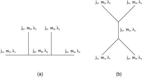
Figure 1: Diagrammatic representation of the conformal blocks for the s-channel (a) and for the t-channel (b).

Notice (see figure 1a) that the fields $1$ and $2$ are attached to the same three-point vertex in ${}^{s}{\cal F}^{1234}_{p}$. Therefore one can assure that $\pi_{12}$ acts diagonally on the s-channel blocks. The same conclusion is valid for $\pi_{34}$ and, thus, we can write:

$$\pi_{12}\,\Bigl{[}\,{}^{s}{\cal F}^{1234}_{p}\,\Bigr{]}\,=\,\Lambda^{p}_{1,2}\,\,\,{}^{s}{\cal F}^{1234}_{p}\,\,\,\,\,\,\,\,\,\,\,\,\,\,\,\,\,\,\,\,\,\,\,\,\,\,\,\,\,\,\,\,\,\,\,\,\,\,\,\,\,\,\,\,\,\,\,\,\,\,\,\,\pi_{34}\,\Bigl{[}\,{}^{s}{\cal F}^{1234}_{p}\,\Bigr{]}\,=\,\Lambda^{p}_{3,4}\,\,\,{}^{s}{\cal F}^{1234}_{p}\,\,,$$ (3.2)

where $\Lambda^{p}_{1,2}$ and $\Lambda^{p}_{3,4}$ are constants. We can also exchange the fields located at positions $2$ and $3$. This is equivalent to the crossing symmetry between the s and u channels. Based on this s-u duality, one can write:

$${}^{s}{\cal F}^{1234}_{p}\,\,=\,\,\sum_{l}\,\,B_{j_{p},j_{l}}\Bigl{[}\,{2\,\,3\atop 1\,\,4}\Bigr{]}\,\,{}^{s}{\cal F}^{1324}_{l}\,\,,$$ (3.3)

where $B_{j_{p},j_{l}}\Bigl{[}\,{2\,\,3\atop 1\,\,4}\Bigr{]}$ are the elements of the so-called braiding matrix [1, 2]. Notice that the different elements of this matrix are labelled by the isospins of the intermediate channels.

One can also use a t-channel basis to describe the space of four-point conformal blocks. These t-channel blocks will be denoted by ${}^{t}{\cal F}^{1234}_{l}$ (see figure 1b). The s-t duality of CFT implies that these basis are related, i.e. that one can write:

$${}^{s}{\cal F}^{1234}_{p}\,\,=\,\,\sum_{l}\,\,F_{j_{p},j_{l}}\Bigl{[}\,{2\,\,3\atop 1\,\,4}\Bigr{]}\,\,{}^{t}{\cal F}^{1234}_{l}\,\,,$$ (3.4)

where the $F\Bigl{[}\,{2\,\,3\atop 1\,\,4}\Bigr{]}$ matrix is the so-called fusion matrix [1, 2].

In order to obtain the explicit form of the duality transformations of eqs. (3.2), (3.3) and (3.4), we shall make use of a free field realization of the osp$(1|2)$ current algebra. This realization was introduced in ref. [7] and used in ref. [9] to study the conformal blocks of the model. Let us describe briefly its basic features. The field content of this representation consists of an scalar field $\phi$, a pair of two conjugate bosonic fields $(w,\chi)$ and two fermionic fields $(\psi,\bar{\psi})$ whose non-vanishing operator product expansions are:

$$w(z_{1})\,\chi(z_{2})\,=\,\psi(z_{1})\,\bar{\psi}(z_{2})\,=\,{1\over z_{1}-z_{2}}\,\,\,\,\,\,\,\,\,\,\,\,\,\,\,\,\,\,\phi(z_{1})\,\phi(z_{2})\,=\,-{\rm log}\,(z_{1}-z_{2})\,.$$ (3.5)

In terms of these fields, one can represent [9] easily the primary fields of the model as:

$$\Phi^{j}_{m}\,=\,\cases{\chi^{j-m}\,e^{-2ij\alpha_{0}\,\phi}&if $j-m\in{\rm Z}\kern-3.8pt{\rm Z}\kern 2.0pt$\cr\cr\chi^{j-m-{1\over 2}}\,\psi\,e^{-2ij\alpha_{0}\,\phi}&if $j-m\in{\rm Z}\kern-3.8pt{\rm Z}\kern 2.0pt\,+{1\over 2}\,$,}$$ (3.6)

where $\alpha_{0}\,=\,-1/\sqrt{2k+3}$. As it is discussed in ref. [9], the representation (3.6) is not unique. In fact, there also exists a conjugate representation which, for a highest weight field, takes the form:

$$\tilde{\Phi}_{j}^{j}\,=\,w^{2j+s}\,\,e^{2i(j+s)\alpha_{0}\,\phi}\,,$$ (3.7)

where $s\,=\,-k-1$. Within this free field approach, the conformal blocks of the model are computed as vacuum expectation values of products of fields of the type (3.6) and (3.7) and an screening charge $Q$, whose expression is:

$$Q\,=\,\oint\,dz\,(\,\bar{\psi}(z)\,-\,w(z)\psi(z)\,)\,e^{i\alpha_{0}\phi(z)}\,.$$ (3.8)

A general four-point block is obtained from a correlator of the form:

$$<\Phi^{j_{1}}_{m_{1}}(z_{1})\,\Phi^{j_{2}}_{m_{2}}(z_{2})\,\Phi^{j_{3}}_{m_{3}}(z_{3})\,\tilde{\Phi}^{j_{4}}_{m_{4}}(z_{4})\,Q^{n}\,>\,,$$ (3.9)

where [9] the number of screening charges is $n\,=\,2\,(\,j_{1}\,+\,j_{2}\,+\,j_{3}\,-\,j_{4}\,)$. The basic information about the duality behaviour of the model can be obtained by studying the block with $j_{3}=j_{2}$ and $j_{4}=j_{1}$ and when the primary fields entering the block are either highest or lowest weights. Due to this fact, we shall restrict ourselves to the situation in which $m_{4}=-m_{1}=j_{1}$ and $m_{2}=-m_{3}=j_{2}$. Moreover, by using the $sl(2)$ projective invariance of the Virasoro algebra, we can fix the positions of the four fields to the values $z_{1}=0$, $z_{2}=z$, $z_{3}=1$ and $z_{4}=\infty$. We shall suppose, finally, that the four representations involved in the correlator (3.9) are even. Therefore, according to these considerations, we have to study the function:

$${\cal F}^{1234}(z)\,\equiv\,<\,\Phi^{j_{1}}_{-j_{1}}(0)\,\Phi^{j_{2}}_{j_{2}}(z)\,\Phi^{j_{2}}_{-j_{2}}(1)\,\tilde{\Phi}^{j_{1}}_{j_{1}}(\infty)\,Q^{4j_{2}}\,>\,.$$ (3.10)

In the framework of this free field representation, the correlator (3.10) can be given as a multiple contour integral of the type:

$${\cal F}^{1234}(z)\,=\,\prod_{i=1}^{n}\,\,\oint_{C_{i}}\,\,d\tau_{i}\,\lambda(z,\{\tau_{i}\})\,\eta(\{\tau_{i}\})\,.$$ (3.11)

In eq. (3.11) (and in what follows), the number $n$ of integrations is $n=4j_{2}$. The function $\lambda(z,\{\tau_{i}\})$ in (3.11) is the contribution of the field $\phi$ to the correlator (3.10). Taking eqs. (3.6) and (3.7) into account, one can write this contribution as:

$$\lambda(z,\{\tau_{i}\})\,=\,<\,e^{-2ij_{1}\alpha_{0}\,\phi(0)} e^{-2ij_{2}\alpha_{0}\,\phi(z)}\,e^{-2ij_{2}\alpha_{0}\,\phi(1)}\,e^{2i(s+j_{1})\alpha_{0}\,\phi(\infty)}\,\times$$ (3.12)

$$\times e^{i\alpha_{0}\,\phi(\tau_{1})}\cdots e^{i\alpha_{0}\,\phi(\tau_{n})}\,>\,.$$

The function $\eta(\{\tau_{i}\})$ in (3.11) represents the contribution of the fields $w$, $\chi$, $\psi$ and $\bar{\psi}$ to (3.10). Using the Fock space selection rules of the free field realization, it was found in ref. [9] that this function can be written as:

$$\eta(\{\tau_{i}\})\, = \,(-1)^{2j_{2}}\,<\,(\chi(0))^{2j_{1}}\,(\chi(1))^{2j_{2}}\,(w(\infty))^{2j_{1}+s}\,w(\tau_{1})\,\cdots\,w(\tau_{2j_{2}})\,\,>\times$$ (3.13)

$$\times\,<\,\psi(\tau_{1})\cdots\psi(\tau_{2j_{2}})\,\bar{\psi}(\tau_{2j_{2}+1})\cdots\bar{\psi}(\tau_{4j_{2}})\,>\,+\,{\rm permutations.}$$

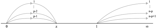
Figure 2: Contours of integration needed to represent ${}^{s}{\cal F}^{1234}_{p}(z)$.

So far we have not specified the contours appearing in eq. (3.11). This specification is equivalent to the choice of a basis in the space of conformal blocks. The contours corresponding to well defined s-channel intermediate states for the blocks (3.11) have been represented in figure 2. We shall take the first $n-p+1$ integrals (whose integration variable will be denoted by $\tau_{i}=u_{i}$ for $i=1,\cdots,n-p+1$) along the contour joining the points $\tau=1$ and $\tau=\infty$ and lying on the real axis. The remaining integration variables will be denoted by $v_{i}$ (i.e.  $v_{i}=\tau_{n-p+1+i}$ for $i=1,\cdots,p-1$ ) and will be integrated in the interval $(0,z)$. All the integrations in a given interval are considered as ordered with respect to the location on the real axis of the singular points of the block (i.e. $\tau=0,z,1$ and $\infty$ ). The ordering along the real line of these singular points is determined by the ordering of the fields in the correlator (3.10). Thus, for example, the first field from the left in eq. (3.10) is evaluated at $\tau=0$, which is also the first point from the left in figure 2. Let us denote by $\lambda_{p}(z,\{u_{i}\},\{v_{i}\})$ and $\eta_{p}(\{u_{i}\},\{v_{i}\})$ the functions $\lambda(z,\{\tau_{i}\})$ and $\eta(\{\tau_{i}\})$ after the relabelling of variables described above. The $p^{{\rm th}}$ s-channel block can be represented as:

$${}^{s}{\cal F}^{1234}_{p}(z)\,=\,\int_{1}^{\infty}\,du_{1}\cdots\int_{1}^{u_{n-p}}\,du_{n-p+1}\int_{0}^{z}\,dv_{1}\cdots\int_{0}^{v_{p-2}}\,dv_{p-1}\,\lambda_{p}(z,\{u_{i}\},\{v_{i}\})\,\eta_{p}(\{u_{i}\},\{v_{i}\}).$$

(3.14)

By using Wick’s Theorem, one can readily evaluate $\lambda_{p}(z,\{u_{i}\},\{v_{i}\})$ with the result:

$$\lambda_{p}(z,\{u_{i}\},\{v_{i}\}) = z^{8j_{1}j_{2}\rho}\,(1-z)^{8j_{2}^{2}\rho}\,\prod_{i=1}^{n-p+1}\,u_{i}^{a}\,(u_{i}-z)^{b}\,(u_{i}-1)^{b}\,\prod_{i<j}(u_{i}-u_{j})^{2\rho}\times$$

$$\times\prod_{i=1}^{p-1}\,v_{i}^{a}\,(z-v_{i})^{b}\,(1-v_{i})^{b}\prod_{i<j}(v_{i}-v_{j})^{2\rho}\,\prod_{i=1}^{n-p+1}\,\prod_{j=1}^{p-1}(u_{i}-v_{j})^{2\rho},$$

where $\rho\,=\,\alpha_{0}^{2}/2\,=\,1/2(2k+3)$ and the constants $a$ and $b$ are defined as $a\,=\,-2j_{1}\alpha_{0}^{2}\,$ and $b\,=\,-2j_{2}\alpha_{0}^{2}\,$. Notice that the phases chosen in the different powers in (LABEL:cuarenta) correspond to the ordering of contours shown in figure 2. The s-channel intermediate isospin $j_{p}$, which corresponds to the $p^{{\rm th}}$ block, can be easily obtained [9] by looking at the $z\rightarrow 0$ behaviour of the function (3.14). One gets:

$$j_{p}\,=\,j_{1}\,+\,j_{2}\,+{1\,-\,p\over 2}\,.$$ (3.16)

It is now possible to study the implementation of the different exchange operations defined at the beginning of this section. Let us, first of all, consider the $\pi_{12}$ operation introduced in eq. (3.1). It is clear that, as the result of acting with $\pi_{12}$, the blocks (3.10) are transformed into:

$${\cal F}^{2134}(z)\,\equiv\,<\,\Phi^{j_{2}}_{j_{2}}(z)\,\Phi^{j_{1}}_{-j_{1}}(0)\,\Phi^{j_{2}}_{-j_{2}}(1)\,\tilde{\Phi}^{j_{1}}_{j_{1}}(\infty)\,Q^{4j_{2}}\,>\,.$$ (3.17)

As in eq. (3.14), one can get an integral representation of the blocks (3.17) for a well-defined s-channel intermediate state. Notice that now the contour ordering corresponding to the correlator (3.17) is the one shown in figure 3. Therefore we can write:

$${}^{s}{\cal F}^{2134}_{p}(z)\,=\,\int_{1}^{\infty}\,du_{1}\cdots\int_{1}^{u_{n-p}}\,du_{n-p+1}\int_{z}^{0}\,d\bar{v}_{1}\cdots\int_{z}^{\bar{v}_{p-2}}\,d\bar{v}_{p-1}\,\bar{\lambda}_{p}(z,\{u_{i}\},\{\bar{v}_{i}\})\,\eta_{p}(\{u_{i}\},\{\bar{v}_{i}\}),$$ (3.18)

where the function $\eta_{p}$ is the same used in eq. (3.14) and $\bar{\lambda}_{p}(z,\{u_{i}\},\{\bar{v}_{i}\})$ is given by:

$$\bar{\lambda}_{p}(z,\{u_{i}\},\{\bar{v}_{i}\}) = (-z)^{8j_{1}j_{2}\rho}\,(1-z)^{8j_{2}^{2}\rho}\,\prod_{i=1}^{n-p+1}\,u_{i}^{a}\,(u_{i}-z)^{b}\,(u_{i}-1)^{b}\,\prod_{i<j}(u_{i}-u_{j})^{2\rho}\times$$

$$\times\prod_{i=1}^{p-1}\,(-\bar{v}_{i})^{a}\,(\bar{v}_{i}-z)^{b}\,(1-\bar{v}_{i})^{b}\prod_{i<j}(\bar{v}_{i}-\bar{v}_{j})^{2\rho}\,\prod_{i=1}^{n-p+1}\,\prod_{j=1}^{p-1}(u_{i}-\bar{v}_{j})^{2\rho},$$

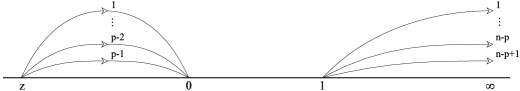
Figure 3: Contours of integration used in the free field representation of ${}^{s}{\cal F}^{2134}_{p}(z)$.

Let us now try to relate the functions (3.14) and (3.18). First of all, it is clear from the contours of figure 3 that the integral (3.18) is naturally defined in the situation in which $z<0$, whereas, on the contrary, the integration limits in (3.14) correspond to the case $z>0$. It is not difficult to analytically continue the expression (3.18) from the $z<0$ domain to the range $z>0$. The first step in this analytical continuation consists in exchanging the upper and lower limits of the $\bar{v}_{i}$ integrations in (3.18):

$$\int_{z}^{0}\,d\bar{v}_{1}\cdots\int_{z}^{\bar{v}_{p-2}}\,d\bar{v}_{p-1}\,[\,\cdots\,]\,=\,(-1)^{p-1}\,\int^{z}_{0}\,d\bar{v}_{1}\cdots\int^{z}_{\bar{v}_{p-2}}\,d\bar{v}_{p-1}\,[\,\cdots\,]\,\,.$$ (3.20)

Notice that, in the right-hand side of eq. (3.20), the variables are ordered as $z>\bar{v}_{p-1}>\bar{v}_{p-2}>\cdots>\bar{v}_{1}>0$. This is not the ordering appearing in the integral (3.14). The latter can be obtained by means of the following redefinition of the $\bar{v}_{i}$ variables:

$$v_{i}\,=\,\bar{v}_{p-i}\,\,\,\,\,\,\,\,\,\,\,\,\,\,\,i=1,\cdots,p-1\,\,.$$ (3.21)

Performing this change of variables in the right-hand side of eq. (3.20) and reversing the order of the iterated integrals in the resulting expression, one gets:

$$\int_{z}^{0}\,d\bar{v}_{1}\cdots\int_{z}^{\bar{v}_{p-2}}\,d\bar{v}_{p-1}\,[\,\cdots\,]\,=\,(-1)^{p-1}\,\int_{0}^{z}\,dv_{1}\cdots\int_{0}^{v_{p-2}}\,dv_{p-1}\,\,[\,\cdots\,]\,\,.$$ (3.22)

Moreover, it is clear from their definitions that, when the relabelling (3.21) is performed, the function $\bar{\lambda}_{p}(z,\{u_{i}\},\{\bar{v}_{i}\})$ is transformed into the function $\lambda_{p}(z,\{u_{i}\},\{v_{i}\})$ multiplied by a phase, while the function $\eta_{p}$ is multiplied by a sign. It is easy to evaluate these factors. The result is:

$$\bar{\lambda}_{p}(z,\{u_{i}\},\{\bar{v}_{i}\}) = e^{8i\pi j_{1}j_{2}\rho}\,e^{i\pi(a+b)(p-1)}\,e^{i\pi(p-1)(p-2)\rho}\,\lambda_{p}(z,\{u_{i}\},\{v_{i}\})$$

$$\eta_{p}(\{u_{i}\},\{\bar{v}_{i}\}) = (-1)^{{(p-1)(p-2)\over 2}}\,\eta_{p}(\{u_{i}\},\{v_{i}\})\,\,.$$ (3.23)

Putting together all the factors appearing in eqs. (3.22) and (3.23), we obtain the explicit expression of $\Lambda_{1,2}^{p}$:

$$\Lambda^{p}_{1,2}\,=\,(-1)^{{p(p-1)\over 2}}\,e^{i\pi\,(h_{j_{p}}\,-\,h_{j_{1}}\,-\,h_{j_{2}})}\,\,,$$ (3.24)

where $h_{j_{1}}$, $h_{j_{2}}$ and $h_{j_{p}}$ are given by eq. (2.5). It is interesting to write the sign in eq. (3.24) in a slightly different form. Let us denote by $<x>$ the integer part of any integer or half-integer number $x$. As $(-1)^{p(p-1)/2}\,=\,(-1)^{<p/2>}$ for any $p\in{\rm Z}\kern-3.8pt{\rm Z}\kern 2.0pt$, and after taking eq. (3.16) into account, eq. (3.24) can be rewritten as:

$$\Lambda^{p}_{1,2}\,=\,(-1)^{<j_{1}+j_{2}-j_{p}+{1\over 2}>}\,e^{i\pi\,(h_{j_{p}}\,-\,h_{j_{1}}\,-\,h_{j_{2}})}\,\,.$$ (3.25)

It is also very interesting to write eq. (3.25) in terms of the deformation parameter $q$, introduced in eq. (2.16). After a short calculation, one concludes that the corresponding expression is:

$$\Lambda^{p}_{1,2}\,=\,(-1)^{<j_{1}+j_{2}-j_{p}+{1\over 2}>}\,q^{j_{p}(2j_{p}+1)\,-\,j_{1}(2j_{1}+1)\,-\,j_{2}(2j_{2}+1)}\,\,.$$ (3.26)

In the form (3.26), the value of $\Lambda^{p}_{1,2}$ has a very neat interpretation. Indeed, one can regard the sign in (3.26) as the classical part of $\Lambda^{p}_{1,2}$ and the power of $q$ as its quantum deformation. The quantum part of $\Lambda^{p}_{1,2}$ is the one expected from the general formalism of CFT [1], whereas the classical contribution should be determined from the (undeformed) ${\rm osp}(1|2)$ representation theory. In general, the state $|\,j_{p},m_{p}>$, obtained by tensor multiplication of two representations of isospins $j_{1}$ and $j_{2}$, is given by an expression of the form:

$$|\,j_{p},m_{p}\,>\,=\,\sum_{m_{1},m_{2}}\,C_{j_{1},m_{1},\lambda_{1};j_{2},m_{2},\lambda_{2}}^{j_{p},m_{p},\lambda_{p}}\,\,\,\,|j_{1},m_{1}>\otimes\,|j_{2},m_{2}>\,\,,$$ (3.27)

where $C_{j_{1},m_{1},\lambda_{1};j_{2},m_{2},\lambda_{2}}^{j_{p},m_{p},\lambda_{p}}$ are the ${\rm osp}(1|2)$ Clebsch-Gordan coefficients. Under the exchange of the two representations in the tensor product, these Clebsch-Gordan coefficients change by a sign. Let us write this behaviour as:

$$C_{j_{2},m_{2},\lambda_{2};j_{1},m_{1},\lambda_{1}}^{j_{p},m_{p},\lambda_{p}}\,\,=\,\,\epsilon_{j_{1},m_{1},\lambda_{1};j_{2},m_{2},\lambda_{2}}^{j_{p},m_{p},\lambda_{p}}\,\,\,\,C_{j_{1},m_{1},\lambda_{1};j_{2},m_{2},\lambda_{2}}^{j_{p},m_{p},\lambda_{p}}\,\,.$$ (3.28)

The $\epsilon_{j_{1},m_{1},\lambda_{1};j_{2},m_{2},\lambda_{2}}^{j_{p},m_{p},\lambda_{p}}$ signs of the right-hand side of (3.28) can be obtained from the values of the Clebsch-Gordan coefficients of ${\rm osp}(1|2)$ [19]. One has:

$$\epsilon_{j_{1},m_{1},\lambda_{1};j_{2},m_{2},\lambda_{2}}^{j_{p},m_{p},\lambda_{p}}\,\,=\,\,\,(-1)^{<j_{1}+j_{2}-j_{p}+{1\over 2}>}(-1)^{(\lambda_{p}+1)(\lambda_{1}+\lambda_{2})+\lambda_{1}\lambda_{2}}\,(-1)^{(\lambda_{1}+2(j_{1}-m_{1}))(\lambda_{2}+2(j_{2}-m_{2}))}\,\,.$$

(3.29)

Notice that, indeed, when $\lambda_{1}\,=\,\lambda_{2}\,=\,0$ and $j_{1}-m_{1}\,,\,j_{2}-m_{2}\in{\rm Z}\kern-3.8pt{\rm Z}\kern 2.0pt$, the signs of the right-hand sides of (3.29) and (3.26) coincide.

It is interesting to point out the dependence on the Cartan eigenvalues $m_{i}$ of the right-hand side of eq. (3.29). This dependence, which does not occur in the su$(2)$ case, has its origin in the sign generated in the exchange of two ${\rm osp}(1|2)$ states due to their different Grassmann parities. It follows that, in general, the eigenvalues in eq. (3.2) will depend on the $m_{i}$’s. It can be checked that, for general Cartan eigenvalues of the fields inserted in the four-point correlator, our free field representation gives rise to the same $m_{i}$ dependence as in eq. (3.29).

The behaviour of the blocks under the exchange operation $\pi_{34}$ can be determined by the same method employed to study the action of $\pi_{12}$. In fact, it is easy to verify that, with the appropriate substitutions, the value of the constants $\Lambda_{3,4}^{p}$ is also given by eq. (3.25). The determination of the braiding matrix defined in eq. (3.3) is much more involved. In general, one has to employ contour manipulation techniques in order to relate the multiple integrals appearing in the free field representation of both sides of eq. (3.3). We shall restrict ourselves here to analyze the braiding matrix of blocks of the type (3.10) with $j_{1}=j_{2}=j$. Let us denote by ${\cal B}^{{j}}$ the $(4j+1)\times(4j+1)$ dimensional matrix that implements the s-u crossing symmetry in the free field representation of this type of blocks. In appendix A, the $j=1/2$ case is worked out. Using the results of this appendix one can write the ${\cal B}^{{1\over 2}}$ matrix as:

$${\cal B}^{{1\over 2}}\,=\,\pmatrix{{q^{2}\over[{3\over 2}]_{+}}&-q&-q^{-1}\,{[{5\over 2}]_{+}\over[{3\over 2}]_{+}}\cr\cr{q\over[{3\over 2}]_{+}}&-{[1]_{+}+[2]_{+}\over[2]_{+}}&-q^{-2}\,{[{5\over 2}]_{+}[1]_{+}\over[2]_{+}[{3\over 2}]_{+}}\cr\cr-{q^{-1}\over[{3\over 2}]_{+}}&{q^{-2}\,[1]_{+}\over[2]_{+}}&-q^{-4}\,{[1]_{+}\over[2]_{+}[{3\over 2}]_{+}}\cr}\,\,,$$ (3.30)

where the graded q-numbers have been defined in eq. (2.17). As a consistency check of eq. (3.30) one can verify that, as expected, when $j_{1}=j_{2}=1/2$, the quantities $\Lambda_{1,2}^{p}$, given in eq. (3.25), are eigenvalues of ${\cal B}^{{1\over 2}}$. Moreover, it is interesting to point out that, performing a change of basis in the space of blocks, the braiding matrix of eq. (3.30) can be recast as a symmetric matrix which is much more convenient for our purposes. Indeed, let us conjugate the braiding matrix ${\cal B}^{{1\over 2}}$ in the form:

$$B^{{1\over 2}}\,=\,\gamma\,{\cal B}^{{1\over 2}}\,\gamma^{-1}\,\,,$$ (3.31)

where $\gamma$ is the following diagonal matrix:

$$\gamma\,=\,\pmatrix{1&&\cr&i\sqrt{\Bigl{[}\,{3\over 2}\,\Bigr{]}_{+}}&\cr&&\sqrt{\Bigl{[}\,{5\over 2}\,\Bigr{]}_{+}}\,\,\cr}\,\,.$$ (3.32)

After the conjugation (3.31), the resulting braiding matrix $B^{{1\over 2}}$ is:

$$B^{{1\over 2}}\,=\,\pmatrix{{q^{2}\over[{3\over 2}]_{+}}&i{q\over\sqrt{[{3\over 2}]_{+}}}&-q^{-1}{\sqrt{[{5\over 2}]_{+}}\over[{3\over 2}]_{+}}\cr\cr i{q\over\sqrt{[{3\over 2}]_{+}}}&-{[1]_{+}+[2]_{+}\over[2]_{+}}&-iq^{-2}\,{[1]_{+}\sqrt{[{5\over 2}]_{+}}\over[2]_{+}\sqrt{[{3\over 2}]_{+}}}\cr\cr-q^{-1}{\sqrt{[{5\over 2}]_{+}}\over[{3\over 2}]_{+}}&-iq^{-2}\,{[1]_{+}\sqrt{[{5\over 2}]_{+}}\over[2]_{+}\sqrt{[{3\over 2}]_{+}}}&-q^{-4}\,{[1]_{+}\over[2]_{+}[{3\over 2}]_{+}}\cr}\,\,.$$ (3.33)

On the other hand, as argued in ref. [17], the fusion matrix for the blocks (3.10) can be obtained by looking at the relation between the functions ${}^{s}{\cal F}^{1234}(z)$ and ${}^{s}{\cal F}^{1234}(1-z)$. In the simplest case, in which $j_{1}=j_{2}=1/2$, the corresponding matrix elements have been explicitly given in ref. [17]. Adapting eq. (5.11) of the first paper in ref. [17] to our case, and after conjugating with the same diagonal matrix $\gamma$ as in eq. (3.32), one arrives at the following symmetric expression:

$$F^{{1\over 2}}\,=\,\pmatrix{-{1\over[{3\over 2}]_{+}}&-{i\over\sqrt{[{3\over 2}]_{+}}}&-{\sqrt{[{5\over 2}]_{+}}\over[{3\over 2}]_{+}}\cr\cr-{i\over\sqrt{[{3\over 2}]_{+}}}&{[1]_{+}+[2]_{+}\over[2]_{+}}&-i{[1]_{+}\sqrt{[{5\over 2}]_{+}}\over[2]_{+}\sqrt{[{3\over 2}]_{+}}}\cr\cr-{\sqrt{[{5\over 2}]_{+}}\over[{3\over 2}]_{+}}&-i{[1]_{+}\sqrt{[{5\over 2}]_{+}}\over[2]_{+}\sqrt{[{3\over 2}]_{+}}}&{[1]_{+}\over[2]_{+}[{3\over 2}]_{+}}\cr}\,\,,$$ (3.34)

where we have denoted by $F^{j}$ the fusion matrix for the blocks (3.10) with $j_{1}=j_{2}=j$.

From the particular cases of $B^{j}$ and $F^{j}$ just found it is not difficult to find out their values for an arbitrary value of the isospin $j$. The key observation in this respect is the comparison between the matrices of eqs. (3.33) and (3.34) and those corresponding to the su$(2)$ CFT. Let us denote by $\tilde{B}^{j}(t)$ and $\tilde{F}^{j}(t)$ the braiding and fusion matrices of the su$(2)$ conformal blocks of correlators of four primary fields with the same isospin $j$. For convenience, we have chosen a notation for these matrices in which the deformation parameter $t$ appears explicitly. As was shown in ref. [3], the su$(2)$ fusion matrices can be put in terms of the Racah-Wigner $6j$ symbols of $U_{t}({\rm su}(2))$. These symbols were computed in ref. [4]. Using these results we can write:

$$\tilde{F}_{j_{1}\,j_{2}}^{\,j}(t)\, = \,(-1)^{j_{1}+j_{2}-2j}\,\,\sqrt{[2j_{1}+1]}\,\sqrt{[2j_{2}+1]}\,\,\Bigl{(}\,\Delta(j,j,j_{1})\,\Delta(j,j,j_{2})\,\Bigr{)}^{2}\,\times$$ (3.35)

$$\times\sum_{m\geq 0}\,\,(-1)^{m}\,[m+1]\,!\,\,\Bigl{(}\,[m-2j-j_{1}]\,!\,\Bigr{)}^{-2}\,\,\Bigl{(}\,[m-2j-j_{2}]\,!\,\Bigr{)}^{-2}\,\,\times$$

$$\times\,\,\Bigl{(}\,[2j+j_{1}+j_{2}-m]\,!\,\Bigr{)}^{-2}\,\,\Bigl{(}\,[4j-m]\,!\,\Bigr{)}^{-1}\,\,.$$

The q-numbers appearing in the right-hand side of eq. (3.35) have been defined in eq. (2.23). The function $\Delta\,(a,b,c)$ is defined as:

$$\Delta\,(a,b,c)\,=\,\sqrt{{[-a+b+c]\,!\,\,[a-b+c]\,!\,\,[a+b-c]\,!\over[a+b+c+1]\,!}}\,\,.$$ (3.36)

Let us now argue that the same identification used in section 2 to pass from the su$(2)$ to the ${\rm osp}(1|2)$ quantum numbers (i.e. $t=-q$) can be utilized to connect the fusion matrices. Actually, our claim is that:

$$F_{j_{1}\,j_{2}}^{j}\,=\,\tilde{F}_{2j_{1}\,2j_{2}}^{\,2j}(-q)\,\,.$$ (3.37)

In order to evaluate the right-hand side of eq. (3.37), we shall use the fact that, when $t=-q$, the quantum factorials are related as:

$$[x]\,!\,=\,(-1)^{x(x-1)\over 4}\,\,\Bigl{[}\,{x\over 2}\,\Bigr{]}_{+}\,!\,\,,$$ (3.38)

where we have denoted:

$$[y]_{+}\,!\,=\,\prod_{j=1/2\atop 2j\,\in\,{\rm Z}\kern-3.8pt{\rm Z}\kern 2.0pt}^{y}\,\,[\,j\,]_{+}\,\,.$$ (3.39)

In terms of the factorials (3.39), we define the function $\Delta_{+}\,(a,b,c)$ by means of the expression:

$$\Delta_{+}\,(a,b,c)\,=\,\sqrt{{[-a+b+c]_{+}\,!\,\,[a-b+c]_{+}\,!\,\,[a+b-c]_{+}\,!\over[a+b+c+{1\over 2}]_{+}\,!}}\,\,.$$ (3.40)

Using these definitions, eq. (3.37) can be written as:

$$F_{j_{1}\,j_{2}}^{j}\, = \,(-1)^{2(j_{1}+j_{2})^{2}\,-\,j_{1}\,-\,j_{2}}\,i^{\,2(j_{1}-<j_{1}>)}\,i^{\,2(j_{2}-<j_{2}>)}\,\,\,\sqrt{\Bigl{[}\,{4j_{1}+1\over 2}\Bigr{]}_{+}}\,\,\sqrt{\Bigl{[}\,{4j_{2}+1\over 2}\Bigr{]}_{+}}\,\times$$

$$\times\,\Bigl{(}\,\Delta_{+}(j,j,j_{1})\,\Delta_{+}(j,j,j_{2})\,\Bigr{)}^{2}\,\sum_{{m\geq 0\atop 2m\in{\rm Z}\kern-3.8pt{\rm Z}\kern 2.0pt}}\,\,(-1)^{m(2m-1)}\,\Bigl{[}{2m+1\over 2}\Bigr{]}_{+}\,!\,\,\Bigl{(}\,[m-2j-j_{1}]_{+}\,!\,\Bigr{)}^{-2}\,\times$$

$$\times\Bigl{(}\,[m-2j-j_{2}]_{+}\,!\,\Bigr{)}^{-2}\,\,\Bigl{(}\,[2j+j_{1}+j_{2}-m]_{+}\,!\,\Bigr{)}^{-2}\,\,\Bigl{(}\,[4j-m]_{+}\,!\,\Bigr{)}^{-1}\,\,.$$

Several remarks concerning eq. (LABEL:sseis) are in order. First of all, one must be specially careful with the $t=-q$ identification in the square root terms of the right-hand side of eq. (3.35), since minus signs are generated inside the square root and one must give a prescription to deal with them. To obtain eq. (LABEL:sseis), we have taken $\sqrt{(-1)^{2x}}$ for $2x\in{\rm Z}\kern-3.8pt{\rm Z}\kern 2.0pt$ to be $i^{2(x-<x>)}$. Moreover, when $F_{j_{1}\,j_{2}}^{j}$ is given by eq. (LABEL:sseis), one can prove a set of properties satisfied by the fusion matrix. The most interesting for our purposes have been compiled in appendix B.

Let us now provide evidence supporting our claim of eq. (3.37). Our first argument is the fact that a direct substitution for $j=1/2$ shows that the matrix elements computed from eq. (LABEL:sseis) coincide with the ones displayed in eq. (3.34). Another piece of evidence is obtained by computing the braiding matrix from eq. (LABEL:sseis). Indeed, a general argument in CFT allows to relate the fusion and braiding matrices [1]. This relation involves the signs (3.29), which encode the behaviour of the Clebsch-Gordan coefficients under the permutation of the two representations that are multiplied in the tensor product. In our case, the relation between the braiding and fusion matrices takes the form:

$$B_{j_{p}j_{l}}\Bigl{[}\,{2\,\,3\atop 1\,\,4}\Bigr{]}\,=\,\epsilon_{j_{3},m_{3},\lambda_{3};j_{4},m_{4},\lambda_{4}}^{j_{p},m_{p},\lambda_{p}}\,\,\,\,\epsilon_{j_{l},m_{l},\lambda_{l};j_{3},m_{3},\lambda_{3}}^{j_{1},m_{1},\lambda_{1}}\,\,\,\,e^{i\pi(h_{j_{1}}+h_{j_{4}}-h_{j_{p}}-h_{j_{l}})}\,\,\,F_{j_{p}j_{l}}\Bigl{[}\,{2\,\,4\atop 1\,\,3}\Bigr{]}\,\,.$$ (3.42)

Taking $j_{1}=j_{2}=j_{3}=j_{4}=j$ and using eq. (3.29) in eq. (3.42), one can prove that:

$$B_{j_{p}j_{l}}^{j}\,=\,(-1)^{2j}\,(-1)^{<j_{p}>}\,(-1)^{<j_{l}>}\,\,q^{4c_{j}-2c_{j_{p}}-2c_{j_{l}}}\,\,F_{j_{p}j_{l}}^{j}\,\,,$$ (3.43)

from which we can obtain the general form of $B^{j}$ once $F^{j}$ is known. One can easily check that, for $j=1/2$, eq. (3.43) reproduces the expression of the braiding matrix elements given in eq. (3.33). For a general value of $j$ one can verify that the eigenvalues of the matrix (3.43) coincide with our free field expression (i.e. with eq. (3.26) for $j_{1}=j_{2}=j$). For low values of $j$ this statement can be checked by an explicit calculation. There is, however, a more powerful indirect argument that makes use of the relation between the matrix $B^{j}$ and its counterpart $\tilde{B}^{\,j}(t)$ in the su$(2)$ theory. The matrix elements of the latter are given in terms of those of the su$(2)$ fusion matrix $\tilde{F}^{\,j}(t)$ by:

$$\tilde{B}_{j_{p}j_{l}}^{\,j}(t)\,=\,(-1)^{j_{p}+j_{l}-2j}\,\,t^{j(j+1)-{j_{p}(j_{p}+1)\over 2}-{j_{l}(j_{l}+1)\over 2}}\,\,\tilde{F}_{j_{p}j_{l}}^{\,j}(t)\,\,.$$ (3.44)

It is not difficult now to prove the following relation between the matrices of eqs. (3.44) and (3.43):

$$B_{j_{p}j_{l}}^{\,j}\,=\,(-1)^{2j}\,\tilde{B}_{2j_{p},2j_{l}}^{\,2j}(-q)\,\,.$$ (3.45)

Eq. (3.45), which was obtained under the assumption that eq. (LABEL:sseis) is correct, implies that the eigenvalues of the matrices $B^{j}$ and $(-1)^{2j}\,\tilde{B}^{\,2j}(-q)$ are equal. As the eigenvalues of $\tilde{B}^{\,j}(t)$, which we shall denote by $\tilde{\Lambda}_{j}^{\,l}(t)$ for $l=0,\cdots,2j$, are known, we can obtain in this way the eigenvalues of $B^{j}$. We are now going to check that the latter agree with the values written in eq. (3.26). Indeed, it is well-known that the $\tilde{\Lambda}_{j}^{\,l}(t)$ are given by:

$$\tilde{\Lambda}_{j}^{\,l}(t)\,=\,(-1)^{2j-l}\,t^{{l(l+1)\over 2}-j(j+1)}\,\,.$$ (3.46)

The eigenvalues of $(-1)^{2j}\,\tilde{B}^{\,2j}(-q)$ are $(-1)^{2j}\,\tilde{\Lambda}_{2j}^{\,2l}(-q)$. A straightforward calculation shows that:

$$(-1)^{2j}\,\tilde{\Lambda}_{2j}^{\,2l}(-q)\,=\,(-1)^{<2j-l+{1\over 2}>}\,q^{l(2l+1)-2j(2j+1)}\,\,,$$ (3.47)

which, for $l=0,\cdots,2j$ and $2l\in{\rm Z}\kern-3.8pt{\rm Z}\kern 2.0pt$, coincide with the set of values given in eq. (3.26). This proves our statement.

4 osp$\bf{(1|2)}$ invariants for torus knots and links

In the previous section we have characterized the exchange symmetry of the ${\rm osp}(1|2)$ CFT. It is nowadays an established fact that there exists a non-trivial connection between the duality properties of two-dimensional CFT’s and three-dimensional topology. The best way to uncover this connection is by formulating a suitable Chern-Simons (CS) topological field theory in three dimensions [6]. This CS theory must be such that, after quantization, its states are in one-to-one correspondence with the conformal blocks of the two-dimensional CFT. In our case there is an obvious choice for the three-dimensional theory. Indeed, since the CFT we are dealing with is endowed of an ${\rm osp}(1|2)$ current algebra, it is natural to consider a theory based on the action:

$$S={k\over 4\pi}\int_{M}{\rm Str}\Big{[}A\wedge dA+{2\over 3}A\wedge A\wedge A\Big{]},$$ (4.1)

where $A$ is a one-form connection taking values in the ${\rm osp}(1|2)$ superalgebra and $M$ is a three-dimensional manifold without boundary. In eq. (4.1), $k$ is a non-negative integer. Once the connection with the two-dimensional theory be established, $k$ will be identified with the level of the ${\rm osp}(1|2)$ affine symmetry.

         

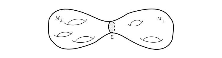
Figure 4: The three dimensional manifold $M$ is split into $M_{1}$ and $M_{2}$, joined along their common boundary $\Sigma$

The basic observables in the CS theories are the Wilson line operators. These are operators defined for each closed curve in $M$ and for each irreducible representation of the superalgebra. For an isospin $j$ representation, the Wilson line operator for a curve $\gamma$ is given by:

$$W_{j}^{\gamma}\,\equiv\,{\rm Str_{j}}\,\Bigl{[}\,P\,{\rm exp}\Bigl{(}\,{\int_{\gamma}\,A}\Bigr{)}\,\Bigr{]}\,\,,$$ (4.2)

where $P$ denotes a path-ordered product along $\gamma$, and the supertrace is taken as the trace over the bosonic states minus the trace over the fermionic states of the isospin $j$ representation of ${\rm osp}(1|2)$. Notice that the operators $W_{j}^{\gamma}$ are both gauge invariant and metric independent.

In order to quantize the theory based on the action (4.1), one must decompose the manifold $M$ as the connected sum of two three-manifolds $M_{1}$ and $M_{2}$ sharing a common boundary $\Sigma$ (see figure 4). In general, the identification of the boundaries of $M_{1}$ and $M_{2}$ will be performed through a homeomorphism. The surface $\Sigma$ in this decomposition will be our equal-time quantization surface. The topological nature of the CS theory allows the possibility of choosing different decompositions of the same three-manifold $M$. The quantum Hilbert space of states of the theory will depend on these decompositions.

The quantization of the CS theory is performed in the presence of Wilson line operators of the type (4.2). In general, the curves on which these Wilson lines are defined can intersect with $\Sigma$. In this case, we shall have on $\Sigma$ a quantization problem with punctures. Each of these punctures is characterized by a representation of the gauge group and by the coordinates of a point of $\Sigma$. According to ref. [6], there exists a correspondence between the CS states on $\Sigma$ and the conformal blocks of a CFT defined on the same two-dimensional surface. These conformal blocks correspond to correlators of fields, with the quantum numbers of the Wilson lines, which are inserted at the points of $\Sigma$ where the intersection with the three-dimensional curves takes place. The interesting aspect from the topological point of view is that the vacuum expectation values of products of Wilson lines are topological invariant and, therefore, one expects that they could be related to some link polynomials. The connection between the CS gauge theory and CFT provides a powerful method to compute these link invariants.

In this section we shall consider the case in which the manifolds $M_{1}$ and $M_{2}$ are two solid tori whose boundary $\Sigma$ is a torus $T^{2}$. We shall assume that the Wilson lines do not intersect with the boundary torus. According to the general arguments reviewed above, the states associated to this two-dimensional quantization surface should be in correspondence with the zero-point conformal blocks of the torus, i.e. with the supercharacters of the model. In what follows we shall verify this fact and we shall find a set of operators which, acting on the torus states, represent the fusion rules of the ${\rm osp}(1|2)$ CFT. Within this approach we shall be able to compute vacuum expectation values of torus links in the three-sphere $S^{3}$. In the next section, based on this result, we shall develop a formalism which will allow us to compute expectation values of more general classes of links.

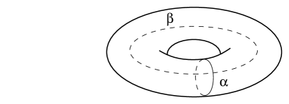
Figure 5: Canonical homology basis for the torus

When $\Sigma=T^{2}$ one can argue, as in ref. [15], that the only relevant components of the connection $A$ on the torus are its zero-modes, which parametrize the holonomy of the gauge field around the non-trivial homology cycles of $T^{2}$. Let us choose a basis for the first homology of the torus as shown in figure 5, in which the $\alpha$ cycle is the one which is contractible in the solid torus. The holomorphic one-form $\omega$ is defined by its integrals along the $\alpha$ and $\beta$ cycles:

$$\int_{\alpha}\,\omega\,=\,1\,\,\,\,\,\,\,\,\,\,\,\,\,\,\int_{\beta}\,\omega\,=\,\tau\,\,,$$ (4.3)

where $\tau$ is the modular parameter of the torus. Since the first homology group of $T^{2}$ is abelian, we can take the zero-mode part of $A$ in the Cartan subalgebra of ${\rm osp}(1|2)$. We shall use the parametrization:

$$A\,=\,{\pi a\over\tau_{2}}\,\bar{\omega}\,J_{0}^{0}\,-\,{\pi\bar{a}\over\tau_{2}}\,\omega\,J_{0}^{0}\,\,,$$ (4.4)

where $\tau_{2}\,=\,{\rm Im}\,\tau$, $a$ and $\bar{a}$ are constants and $J_{0}^{0}$ is the ${\rm osp}(1|2)$ Cartan generator. In the framework of the path integral quantization of the CS action (4.1), one can formulate [15] an effective problem for the zero-modes of the gauge field. One of the outcomes of this formalism is the fact that, in the effective theory, the coefficient $k$ of the CS action is shifted by $c_{v}$, the quadratic Casimir in the adjoint representation. For the ${\rm osp}(1|2)$ superalgebra, $c_{v}$ is equal to $3/2$ and, therefore, the above-mentioned shift is $k\rightarrow k+{3\over 2}$. The states appearing in the zero-mode problem are functions of the variable $a$, whose form can be obtained by solving the Gauss law associated to the action (4.1). In fact, adapting the result of ref. [15] to our ${\rm osp}(1|2)$ case, one can readily prove that the states are given by the numerator of the supercharacters (2.11) multiplied by a convenient prefactor. These functions are:

$$\xi_{j,k}(a,\tau)\,\equiv\,e^{{\pi(2k+3)\over 8\tau_{2}}\,a^{2}}\,\,[\,\,\vartheta_{4j+1,2k+3}(a,\tau)\,-\,\vartheta_{-4j-1,2k+3}(a,\tau)\,\,]\,\,,$$ (4.5)

where $j$ is integer or half integer. From the periodicity properties of the characters (eq. (2.13)), one can immediately conclude that there only exist $k+1$ independent states in the effective Hilbert space whose wavefunctions are given by $\xi_{j,k}(a,\tau)$ for $j=0,{1\over 2},\cdots,{k\over 2}$.

It is not difficult to obtain the operator realization of the gauge field (4.4) in the Hilbert space spanned by the functions (4.5). Actually, the canonical commutation relations corresponding to the action (4.1), after taking into account the $k\rightarrow k+{3\over 2}$ shift, determine the commutator of the zero-mode components of the gauge field. This commutator is:

$$[\,\bar{a}\,,\,a\,]\,=\,{4\tau_{2}\over\pi(2k+3)}\,\,,$$ (4.6)

which implies that $\bar{a}$ can be represented as:

$$\bar{a}\,=\,{4\tau_{2}\over\pi(2k+3)}\,{\partial\over\partial a}\,\,.$$ (4.7)

Using eqs. (4.3), (4.4) and (4.7) one can easily find the expression of the Wilson line operators in terms of $a$ and $\partial/\partial a$. Actually, this can only be done for Wilson line operators corresponding to torus knots, i.e. for curves that can be drawn on the surface of $T^{2}$ without self-intersections. Let $\gamma_{r,s}$ be a torus knot on $T^{2}$ which belongs to the same homology class as $r\alpha+s\beta$, for two coprime integers $r$ and $s$. We shall denote by $W_{j}^{(r,s)}$ the Wilson line operator (4.2) for $\gamma=\gamma_{r,s}$. If $\Lambda_{j}$ represents the set of eigenvalues of the Cartan generator $J_{0}^{0}$ in the isospin $j$ representation, i.e. the $4j+1$ values $\Lambda_{j}\,=\,\{\,j-{p\over 2}\,,\,p=0\,\cdots\,,4j\}$, the expression of the $W_{j}^{(r,s)}$ operator is given by:

$$W_{j}^{(r,s)}\,=\,\sum_{n\in\Lambda_{j}}\,\,(-1)^{2(j-n)}\,\,{\rm exp}\,\Bigl{[}\,{n\pi(r+s\bar{\tau})\over\tau_{2}}\,a\,-\,{4n(r+s\tau)\over 2k+3}\,{\partial\over\partial a}\,\Bigr{]}\,\,.$$ (4.8)

It is not difficult to obtain the action of the operators of eq. (4.8) on the states $\xi_{j,k}(a,\tau)$. The result is:

$$W_{l}^{(r,s)}\,\xi_{j,k}(a,\tau)\,=\,(-1)^{2l}\,\sum_{n\in\Lambda_{l}}\,(-1)^{2n(s-1)}\,q^{4rsn^{2}\,+\,2(4j+1)nr}\,\,\xi_{j+ns,k}(a,\tau)\,\,,$$ (4.9)

where $q$ is the same as in eq. (2.16). In order to prove eq. (4.9) one has to use the well-known behaviour of the theta functions under shifts in their arguments. Notice that, remarkably, the action of the operators (4.8) does not take us out of the Hilbert space spanned by the functions (4.5).

Two particular cases of (4.9) will be of great interest for our purposes. First of all, let us consider the situation in which $r=0$ and $s=1$, i.e. a Wilson line along the $\beta$ cycle of the torus. Eq. (4.9) particularized to this case gives:

$$W_{l}^{(0,1)}\,\xi_{j,k}(a,\tau)\,=\,(-1)^{2l}\,\sum_{n\in\Lambda_{l}}\,\xi_{j+n,k}(a,\tau)\,\,.$$ (4.10)

If one takes $j=0$ in (4.10), which corresponds to acting with $W_{l}^{(0,1)}$ on the vacuum state, one easily arrives at:

$$W_{l}^{(0,1)}\,\xi_{0,k}(a,\tau)\,=\,(-1)^{2l}\,\xi_{l,k}(a,\tau)\,\,.$$ (4.11)

In order to prove eq. (4.11) from eq. (4.10), one has to make use of the periodicity properties of the characters (eq. (2.13)). Eq. (4.11) suggests the interpretation of $W_{l}^{(0,1)}$ as a creation operator of the state $\xi_{l,k}(a,\tau)$. Notice, however, the $(-1)^{2l}$ sign appearing in the right-hand side of eq. (4.11). We can absorb this sign by defining new operators in the form:

$$\Phi_{l}^{(r,s)}\,\equiv\,(-1)^{2l}\,W_{l}^{(r,s)}\,\,.$$ (4.12)

The operators $\Phi_{j}^{(r,s)}$ are the Verlinde operators [18] for the torus Hilbert space. Indeed, as the result of the action of $\Phi_{j}^{(0,1)}$ on the vacuum state $\xi_{0,k}$, the state $\xi_{j,k}$ of isospin $j$ is obtained. Moreover, it can be checked from (4.10) that the operators $\Phi_{j}^{(0,1)}$ satisfy the ${\rm osp}(1|2)$ fusion rules of eq. (2.6). It is interesting to point out that, on the contrary, the Wilson line operators $W_{l}^{(0,1)}$ do not satisfy these fusion rules. Actually, the composition law which they obey has signs. The redefinition of eq. (4.12) eliminates these signs and, as a consequence, the correct fusion rules are reproduced. It is important to point out here the difference with the situation for bosonic gauge groups, where the representation of the Verlinde operators is given directly by the Wilson lines.

Another interesting particular case of eq. (4.9) is $r=1$, $s=0$, which corresponds to Wilson lines for the $\alpha$ cycle of the torus. It follows from (4.9) that, in this case, the Wilson line operators act diagonally on the states (4.5):

$$W_{l}^{(1,0)}\,\xi_{j,k}(a,\tau)\,=\,\sum_{n\in\Lambda_{l}}\,(-1)^{2(l+n)}\,q^{2(4j+1)\,n}\,\xi_{j,k}(a,\tau)\,\,.$$ (4.13)

Remarkably enough, one can show that the alternate sum appearing in the right-hand side of eq. (4.13) can be put in terms of ratios of the entries of the modular matrix $S$:

$$W_{l}^{(1,0)}\,\xi_{j,k}(a,\tau)\,=\,(-1)^{2l}\,{S_{lj}\over S_{0j}}\,\ \xi_{j,k}(a,\tau)\,\,.$$ (4.14)

Notice from eq. (4.14) that the action of $W_{l}^{(1,0)}$ on the vacuum state $\xi_{0,k}$ is equivalent to a multiplication of the latter by the quantum dimension $SD_{q}[l]$(see eq. (2.22)). Another interesting consequence of eq. (4.14) is the fact that the Verlinde operators $\Phi_{l}^{(1,0)}$ also act diagonally on the states (4.5). This is, actually, the content of the Verlinde theorem, which states that the modular $S$ matrix diagonalizes the fusion rules.

Our formalism can be used to compute vacuum expectation values of Wilson lines on the three-sphere $S^{3}$. In this calculation, we shall make use of the well-known fact that the three-sphere $S^{3}$ can be obtained by joining together two solid tori whose boundaries are identified by means of a modular $S$ transformation. This $S$ transformation has a well-defined realization in our Hilbert space. Actually, its matrix elements are precisely the ones displayed in eq. (2.15). The expectation values of Wilson line operators in the vacuum, when the total three manifold is $S^{3}$, can be simply obtained by inserting the $S$ transformation as follows:

$$<\,W_{j}^{(r,s)}\,>_{S^{3}}\,\,=\,\,{(\,SW_{j}^{(r,s)}\,)_{00}\over S_{00}}\,\,.$$ (4.15)

Notice that, in eq. (4.15), we have normalized the vacuum expectation values in such a way that they take the value one for the unit operator (i.e. when $j=0$ in (4.15)). It is understood in the right-hand side of eq. (4.15) that one is taking the diagonal matrix element with respect to the vacuum state $\xi_{0,k}$. Using the results of eqs. (2.15) and (4.9), it is straightforward to compute these matrix elements. One gets:

$$<\,W_{j}^{(r,s)}\,>_{S^{3}}\,\,=\,\,\sum_{n\in\Lambda_{j}}\,(-1)^{2(j+n)}\,q^{4rsn^{2}+2nr}\,\,{\,q^{{4sn+1\over 2}}\,+\,q^{-{4sn+1\over 2}}\over q^{{1\over 2}}\,+\,q^{-{1\over 2}}}\,\,.$$ (4.16)

The sum over $\Lambda_{j}$ appearing in the right-hand side of eq. (4.16) can be done explicitly in some cases. For example, if $s=1$, i.e. for torus knots of type $(r,1)$, one can easily verify that eq. (4.16) reduces to:

$$<\,W_{j}^{(r,1)}\,>_{S^{3}}\,\,=\,\,q^{2j(2j+1)r}\,{\,q^{{4j+1\over 2}}\,+\,q^{-{4j+1\over 2}}\over q^{{1\over 2}}\,+\,q^{-{1\over 2}}}\,\,.$$ (4.17)

Eq. (4.17) contains very interesting information. Let us take, first of all, the case $r=0$. The $(0,1)$ torus knot is nothing but the unknot. On the other hand, it is evident from (4.17) and (2.17) that:

$$<\,W_{j}^{{\rm unknot}}\,>_{S^{3}}\,=\,\Bigl{[}\,{4j+1\over 2}\,\Bigr{]}_{+}\,=\,SD_{q}[j]\,\,.$$ (4.18)

Therefore, as happens for the CS theories with bosonic gauge groups, the expectation values of unknot Wilson lines are the quantum dimensions. Notice, however, that these expectation values are not given by ratios of $S$ matrix elements (see eq. (2.22)). This only occurs when we take expectation values of the Verlinde operators (4.12) for the unknot. It is also interesting to look at the $r$ dependence of the right-hand side of eq. (4.17). This dependence can be written as:

$$<\,W_{j}^{(r,1)}\,>_{S^{3}}\,\,=\,\,e^{2\pi ih_{j}r}\,<\,W_{j}^{(0,1)}\,>_{S^{3}}\,\,,$$ (4.19)

where $h_{j}$ are the conformal weights (2.5).

Two knots or links are isotopically equivalent if they can be transformed into each other by means of a series of moves. The notion of isotopic equivalence depends on the type of moves considered as basic deformations. In knot theory, Reidemeister introduced three basic moves (denoted usually by I, II and III) which define an equivalence relation called ambient isotopy [24]. If one does not include the type I Reidemeister move in the equivalence relation, another notion of topological equivalence, the so-called regular isotopy, is defined [24]. The $(r,1)$ torus knot is ambient isotopy equivalent to the unknot. This fact is illustrated in figure 6, where it is shown how one can convert the $(r,1)$ torus knot into the unknot by means of $r$ type I Reidemeister moves.

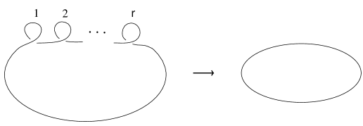
Figure 6: The $(r,1)$ torus knot is transformed into the unknot by means of $r$ Reidemeister moves of type I

As is shown in eq. (4.19), the vacuum expectation value on $S^{3}$ of the Wilson line $W_{j}^{(r,1)}$ depends on $r$ and, therefore, this means that $<\,W_{j}^{(r,1)}\,>_{S^{3}}$ is not invariant under ambient isotopy. This is, actually, a general feature of CS gauge theories which is usually interpreted as due to the fact that the CS theory introduces a frame to the knots along which Wilson lines are defined. Notice that the framing dependence is a multiplicative factor depending on the conformal weight $h_{j}$ of the ${\rm osp}(1|2)$ current algebra. This means that the effect of framing is controlled by the monodromy behaviour of the CFT conformal blocks. For a general $(r,s)$ torus knot, it is clear that the effect due to framing will be a factor $exp[2\pi irsh_{j}]=q^{2j(2j+1)rs}$. The knot polynomials associated to our ${\rm osp}(1|2)$ gauge theory can be obtained by extracting this factor. They are polynomials in the variable $q$ defined as:

$$P_{j}^{{(r,s)}}\,(q)\,\equiv\,q^{2j(2j+1)rs}\,\,{<\,W_{j}^{(-r,s)}\,>_{S^{3}}\over<\,W_{j}^{(0,1)}\,>_{S^{3}}}\,\,.$$ (4.20)

Notice that in the right-hand side of eq. (4.20) we have changed the sign of $r$ in order to adequate our orientation conventions for torus knots to the standard ones in the mathematics literature [24]. We have normalized the knot polynomial in such a way that the polynomial of the unknot is 1. Using the result written in eq. (4.16), it is now straightforward to obtain the following expression of the polynomial for a general torus knot:

$$P_{j}^{{(r,s)}}\,(q)\,=\,{q^{2j(r-1)(s-1)}\over q^{4j+1}+1}\,\,\sum_{p=0}^{4j}\,\,(-1)^{p}\,q^{r(1+sp)(4j-p)}\,\,(\,q^{1+sp}\,+\,q^{s(4j-p)}\,)\,\,.$$ (4.21)

From eq. (4.21), it is easy to find the relation between the ${\rm osp}(1|2)$ and su$(2)$ polynomials. It is interesting to point out that this relation can be obtained by using the same identification of the deformation parameters of $U_{q}({\rm osp}(1|2))$ and $U_{t}({\rm su}(2))$ that was found in sections 2 and 3. Indeed, let $\tilde{P}_{j}^{{(r,s)}}\,(t)$ be the su$(2)$ polynomial of isospin $j$, in the variable $t$, for an $(r,s)$ torus knot. The explicit expressions of the su$(2)$ polynomials for torus knots were obtained in ref. [25]. Comparing these results with eq. (4.21), one easily realizes that:

$$P_{j}^{{(r,s)}}\,(q)\,=\,\tilde{P}_{2j}^{{(r,s)}}\,(-q)\,\,.$$ (4.22)

Notice that eq. (4.22) implies that our ${\rm osp}(1|2)$ polynomials can be identified with the su$(2)$ polynomials for integer isospins. Therefore, for example, the ${\rm osp}(1|2)$ polynomial for the fundamental representation is identified in eq. (4.22) with the Akutsu-Wadati polynomial obtained from the three-state vertex model (i.e. from the nineteen-vertex model) [26]. So far we have only related ${\rm osp}(1|2)$ and su$(2)$ polynomials for torus knots. In next section we shall be able to verify this relation for more general classes of knots of links. Within our present formalism, we can generalize eq. (4.22) to arbitrary torus links. Let us remember that, in general, an $(r,s)$ torus link can be represented as the closure of the braid with $s$ strands $(\sigma_{1}\,\cdots\,\sigma_{s-1})^{r}$, where $\sigma_{i}$ is the operation that interchanges the strands numbered $i$ and $i+1$. When $r$ and $s$ are coprime, the link is an $(r,s)$ torus knot. On the contrary, when the greatest common divisor of $r$ and $s$, which we shall denote by $gcd(r,s)$, is different from one, the link has more that one component. In fact, it is not difficult to convince oneself that the number of components of the $(r,s)$ torus link is given precisely by:

$$\nu_{r,s}\,=\,gcd(r,s)\,\,.$$ (4.23)

Furthermore, one can verify that each of the $\nu_{r,s}$ components of the link is an $(r/\nu_{r,s}\,,\,s/\nu_{r,s})$ torus knot.

The polynomial for a link can be obtained by means of a slight generalization of our prescription for knots (eq. (4.20)). Basically, one must compute the expectation value of a product of more that one Wilson line operators. Actually, one must insert in the correlator a Wilson line operator for every component of the link. Taking into account the framing factor, these considerations lead us to define the polynomial for an $(r,s)$ torus link as [25]:

$$P^{(r,s)}_{j}(q)={q^{2j(2j+1)rs}\over{\langle W^{(0,1)}_{j}\rangle}_{S^{3}}}\,\,\Bigl{\langle}\,\Biggl{(}W^{(-{r\over\nu_{r,s}}\,,\,{s\over\nu_{r,s}})}_{j}\Biggr{)}^{\nu_{r,s}}\,\Bigr{\rangle}_{S^{3}}.$$ (4.24)

The calculation of the right-hand side of eq. (4.24) can be performed by using the same techniques as in ref. [25]. If $\tilde{P}^{(r,s)}_{j}(t)$ is the su$(2)$ polynomial for an $(r,s)$ torus knot in the isospin $j$ representation, one can prove that:

$$P^{(r,s)}_{j}(q)\,=\,(-1)^{2j(\nu_{r,s}-1)}\,\,\tilde{P}^{(r,s)}_{2j}(-q)\,\,.$$ (4.25)

The values of the su$(2)$ polynomials for torus links were given in ref. [25] and will not be reproduced here. Notice that now, in eq. (4.25), apart from the $q\rightarrow-q$, $j\rightarrow 2j$ correspondence, there appears a $(-1)^{2j}$ sign, which was not present in the case of knots. In next section we shall develop an approach which will allow us to confirm this ${\rm osp}(1|2)/{\rm su}(2)$ connection for arbitrary links.

5 osp$\bf{(1|2)}$ invariants for arbitrary knots and links

The topological nature of CS gauge theories allows to describe a given three-dimensional situation in terms of different two-dimensional problems. Exploiting this richness of the CS theories, a series of powerful computational techniques can be developed. Indeed, as we recalled at the beginning of section 4, in the quantization of the CS theory on the three-sphere, one must split $S^{3}$ as a connected sum of two three-manifolds with a common boundary $\Sigma$. In section 4 we have been considering the particular case in which $\Sigma=T^{2}$ and there are no Wilson lines cut by the intermediate torus. In the present section, we shall cut the $S^{3}$ manifold along a two-sphere $S^{2}$, chosen in such a way that it intersects the Wilson lines in four points. In order to characterize the CS states in these punctured two-spheres, we shall make use of the results of section 3 on the behaviour under crossing symmetry of the four-point conformal blocks in the ${\rm osp}(1|2)$ CFT.

         

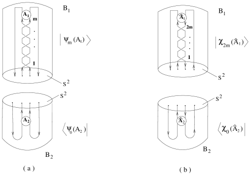
Figure 7: Composition of balls $B_{1}$ and $B_{2}$ which yields the links $L_{m}\,(A_{1}\,,\,A_{2}\,)$ (a) and $\hat{L}_{2m}\,(\hat{A}_{1}\,,\,\hat{A}_{2}\,)$ (b) in $S^{3}$.

Let us build up our formalism, following ref. [16]. First of all, we shall introduce some definitions. We shall call a compact three-dimensional submanifold in $S^{3}$ with some points of the boundary marked as “in” or “out”, a “room” [27]. An “inhabitant” of the room is, by definition, a properly embedded smooth, compact oriented one-dimensional manifold which meets the boundary of the room at the given set of marked points with its orientation matching the “in” and “out” designations. Given two rooms $A_{1}$ and $A_{2}$ with two “in” and two “out” points, let us consider the link $L_{m}\,(A_{1}\,,\,A_{2}\,)$, obtained by joining $A_{1}$ and $A_{2}$ by four strands, with $m$ half-twists in two of the parallelly oriented strands. In figure 7a, we have represented the embedding of $L_{m}\,(A_{1}\,,\,A_{2}\,)$ in $S^{3}$. As shown in this figure, we shall decompose $S^{3}$ into two solid balls $B_{1}$ and $B_{2}$ in such a way that $B_{1}$ contains the room $A_{1}$ and the $m$ half-twists in its parallel strands and $B_{2}$ contains the room $A_{2}$. Notice that the common boundary $S^{2}$ intersects with the four strands and that the lower two strands of $A_{1}$ and $A_{2}$ are parallelly oriented. We shall also consider the links $\hat{L}_{2m}\,(\hat{A}_{1}\,,\,\hat{A}_{2}\,)$, where $\hat{A}_{1}$ and $\hat{A}_{2}$ are rooms whose lower two strands have opposite orientation. The link $\hat{L}_{2m}\,(\hat{A}_{1}\,,\,\hat{A}_{2}\,)$ is obtained, as shown in figure 7b, by joining the rooms $\hat{A}_{1}$ and $\hat{A}_{2}$ with four strands, with $2m$ half-twists in the oppositely oriented lower two strands of $\hat{A}_{1}$.

Let us now describe how one can obtain the ${\rm osp}(1|2)$ polynomials for the links of figure 7. We are going to consider first the link $L_{m}\,(A_{1}\,,\,A_{2}\,)$. As shown in figure 7a, one can associate a state to each of the two balls $B_{1}$ and $B_{2}$ in which $S^{3}$ is split. These states, denoted by $|\,\psi_{m}(A_{1})\,>$ and $<\psi_{0}(A_{2})\,|$, can be obtained by performing the CS functional integral over the balls $B_{1}$ and $B_{2}$ respectively. The expectation value of the link will be given by the inner product of these two states. The corresponding invariant polynomial can be obtained after extracting the framing dependence and after performing a convenient normalization. Therefore, if we denote the isospin $j$ polynomial of the link by $P_{j}\,[\,L_{m}\,(A_{1}\,,\,A_{2}\,)\,]\,(q)$, it is clear that:

$$P_{j}\,[\,L_{m}\,(A_{1}\,,\,A_{2}\,)\,]\,(q)\,=\,{<\psi_{0}(A_{2})\,|\,\psi_{m}(A_{1})\,>\over SD_{q}[j]}\,\,.$$ (5.1)

In eq. (5.1), we have taken into account the result (4.18) for the expectation value of the unknot. The dependence of the right-hand side of eq. (5.1) in the number $m$ of twists can be obtained as follows. Let $B_{j}^{(+)}$ be the operator that introduces a frame corrected half twist in the middle two strands of the CS states on $S^{2}$. Obviously, the action of $B_{j}^{(+)}$ on the states is:

$$B_{j}^{(+)}\,|\,\psi_{l}(A_{1})\,>\,=\,|\,\psi_{l+1}(A_{1})\,>\,\,.$$ (5.2)

It is interesting for our purposes to introduce the eigenvectors $|\,\phi_{l}^{(+)}\,>$ of the $B_{j}^{(+)}$ operator:

$$B_{j}^{(+)}\,|\,\phi_{l}^{(+)}\,>\,=\,\Lambda_{l,j}^{(+)}\,(q)\,|\,\phi_{l}^{(+)}\,>\,\,.$$ (5.3)

From our analysis of the four-point conformal blocks of the ${\rm osp}(1|2)$ CFT (sect. 3), it is clear that $B_{j}^{(+)}$ acts in a $4j+1$-dimensional space. Actually, we shall label the braiding eigenstates and eigenvalues as in section 3 and, therefore, $l$ in eq. (5.3) will take the values $l\,=\,0,\cdots,2j$ with $2l\in{\rm Z}\kern-3.8pt{\rm Z}\kern 2.0pt$. Let us denote the braiding eigenvalues of eq. (3.26) for $j_{1}=j_{2}=j$ and $j_{p}=l$ by $\Lambda_{j}^{l}(q)$. After taking into account the framing corrections (eq. (4.19)) and our orientation conventions (eq. (4.20)), it is clear that:

$$\Lambda_{l,j}^{(+)}(q)\,=\,exp[\,2\pi ih_{j}\,]\,\Lambda_{j}^{l}(q^{-1})\,\,.$$ (5.4)

Therefore, making use of eq. (3.26), one can write:

$$\Lambda_{l,j}^{(+)}(q) = (-1)^{<2j-l+{1\over 2}>}\,q^{4j(2j+1)-l(2l+1)}$$

$$l\, = \,0,\cdots,2j,\,\,\,\,\,\,\,\,\,\,\,\,\,\,\,\,\,\,\,2l\in{\rm Z}\kern-3.8pt{\rm Z}\kern 2.0pt\,\,.$$ (5.5)

With the eigenvalues (5.5) at our disposal, we can use the characteristic equation of $B_{j}^{(+)}$ in order to get recursion relations (skein rules) that the ${\rm osp}(1|2)$ polynomials must obey. However, these skein rules, which relate the polynomials (5.1) for different values of $m$, cannot completely determine the CS invariants for arbitrary knots and links. Fortunately, as was shown in ref. [16], the polynomials can be directly obtained from the monodromy properties of the two-dimensional four-point correlators. Indeed, if we expand the vectors appearing in the decomposition of figure 7a for $m=0$ as:

$$|\,\psi_{0}(A_{1})\,>\, = \,\sum_{{l=0\atop 2l\in{\rm Z}\kern-3.8pt{\rm Z}\kern 2.0pt}}^{2j}\,\,\mu_{l}^{(+)}(A_{1})\,|\,\phi_{l}^{(+)}\,>$$

$$<\,\psi_{0}(A_{2})\,|\, = \,\sum_{{l=0\atop 2l\in{\rm Z}\kern-3.8pt{\rm Z}\kern 2.0pt}}^{2j}\,\,\mu_{l}^{(+)}(A_{2})\,<\,\phi_{l}^{(+)}\,|\,\,,$$ (5.6)

then, using eqs. (5.2) and (5.3), the state $|\,\psi_{m}(A_{1})\,>$ can be written as:

$$|\,\psi_{m}(A_{1})\,>\,=\,\sum_{{l=0\atop 2l\in{\rm Z}\kern-3.8pt{\rm Z}\kern 2.0pt}}^{2j}\,\,\mu_{l}^{(+)}(A_{1})\,[\,\Lambda_{l,j}^{(+)}\,(q)\,]^{m}\,|\,\phi_{l}^{(+)}\,>\,\,.$$ (5.7)

In eq. (5.6), $\mu_{l}^{(+)}(A_{1})$ and $\mu_{l}^{(+)}(A_{2})$ are certain coefficients which depend on the rooms $A_{1}$ and $A_{2}$. The states $|\,\phi_{l}^{(+)}\,>$, $l=0,\cdots,2j$ can be chosen in such a way that they form a complete orthonormal set. Therefore, their inner product with the elements $<\,\phi_{l}^{(+)}\,|$ of the dual basis is given by $<\,\phi_{m}^{(+)}\,|\,\phi_{l}^{(+)}\,>\,=\,\delta_{ml}$. Using this fact, one can write the following expression for the polynomial of the link $L_{m}\,(A_{1}\,,\,A_{2}\,)$:

$$P_{j}\,[\,L_{m}\,(A_{1}\,,\,A_{2}\,)\,]\,(q)\,=\,{1\over SD_{q}[j]}\,\,\sum_{{l=0\atop 2l\in{\rm Z}\kern-3.8pt{\rm Z}\kern 2.0pt}}^{2j}\,\,\mu_{l}^{(+)}(A_{1})\,\mu_{l}^{(+)}(A_{2})\,[\,\Lambda_{l,j}^{(+)}\,(q)\,]^{m}\,\,.$$ (5.8)

Notice that, in eq. (5.8), the dependence of $P_{j}\,[\,L_{m}\,(A_{1}\,,\,A_{2}\,)\,]\,(q)$ on the number $m$ of half-twists has been explicitly determined. However, we need to obtain the coefficients appearing in the linear combinations (5.6) in order to get the actual expression of the polynomial. Let us consider, first of all, the case in which $A_{1}$ and $A_{2}$ are the “trivial” rooms, i.e. when $A_{1}$ and $A_{2}$ are:

         
(5.9)

When $A_{1}$ and $A_{2}$ are the rooms (5.9), the link $L_{m}\,(A_{1}\,,\,A_{2}\,)$ is simply the link ${\cal L}_{m}$ obtained as the closure of an $m$-twisted braid of two parallelly oriented strands. Notice that ${\cal L}_{m}$ is nothing but the $(m,2)$ torus link, which has one(two) components when $m$ is odd(even). If we denote by $\mu_{l}^{(+)}$ the coefficients $\mu_{l}^{(+)}(A_{1})$ and $\mu_{l}^{(+)}(A_{2})$ when $A_{1}$ and $A_{2}$ are given by (5.9), it is evident that, in this case, eq. (5.8) reduces to:

$$P_{j}^{(m,2)}(q)\,=\,P_{j}\,[\,{\cal L}_{m}\,](q)\,=\,{1\over SD_{q}[j]}\,\,\sum_{l=0\atop 2l\,\in\,{\rm Z}\kern-3.8pt{\rm Z}\kern 2.0pt}^{2j}\,[\,\mu_{l}^{(+)}\,]^{2}\,[\,\Lambda_{l,j}^{(+)}(q)\,]^{m}\,\,.$$ (5.10)

We have determined the expression of $P_{j}^{(m,2)}(q)$ in section 4 (see eq. (4.21) for knots and eq. (4.25) in the case of links). It can be easily proved that the results of section 4 can be written as:

$$P_{j}^{(m,2)}(q)\,=\,{1\over SD_{q}[j]}\,\,\sum_{l=0\atop 2l\,\in\,{\rm Z}\kern-3.8pt{\rm Z}\kern 2.0pt}^{2j}\,(-1)^{2l}\,\Bigl{[}\,{4l+1\over 2}\,\Bigr{]}_{+}\,(-1)^{m<2j-l+{1\over 2}>}\,q^{m[4j(2j+1)-l(2l+1)]}\,\,.$$ (5.11)

In the right-hand side of eq. (5.11), one can immediately recognize the $m^{{\rm th}}$ power of the braiding eigenvalue $\Lambda_{l,j}^{(+)}(q)$. Therefore, the $\mu_{l}^{(+)}$ coefficients satisfy:

$$[\,\mu_{l}^{(+)}\,]^{2}\,=\,(-1)^{2l}\,\Bigl{[}\,{4l+1\over 2}\,\Bigr{]}_{+}\,\,,$$ (5.12)

which means that the $\mu_{l}^{(+)}$ are given by:

$$\mu_{l}^{(+)}\,=\,i^{2(l-<l>)}\,\sqrt{\Bigl{[}\,{4l+1\over 2}\,\Bigr{]}_{+}}\,\,.$$ (5.13)

Later in this section we shall use the result (5.13) to determine the CS states associated to general classes of rooms.

Let us now consider the link $\hat{L}_{m}\,(\hat{A}_{1}\,,\,\hat{A}_{2}\,)$ represented in 7b. It is clear that, in this case, the corresponding polynomial is:

$$P_{j}\,[\,\hat{L}_{2m}\,(\hat{A}_{1}\,,\,\hat{A}_{2}\,)\,]\,(q)\,=\,{<\chi_{0}(\hat{A}_{2})\,|\,\chi_{2m}(\hat{A}_{1})\,>\over SD_{q}[j]}\,\,.$$ (5.14)

We can evaluate the right-hand side of eq. (5.14) following the same strategy used to arrive at eq. (5.8). Let us introduce the operator $B_{j}^{(-)}$ that implements the half-twists in the oppositely oriented middle two strands on the ball $B_{1}$ in figure 7b. As in the case of $B_{j}^{(+)}$, we shall assume that in the action of $B_{j}^{(-)}$ the framing dependence has been eliminated. In analogy with eq. (5.2), one has $|\,\chi_{2m}(\hat{A}_{1})\,>\,=\,[\,B_{j}^{(-)}\,]^{2m}\,|\,\chi_{0}(\hat{A}_{1})\,>$. Let us also introduce a complete set of orthonormal eigenstates of $B_{j}^{(-)}$:

$$B_{j}^{(-)}\,|\,\phi_{l}^{(-)}\,>\,=\,\Lambda_{l,j}^{(-)}\,(q)\,|\,\phi_{l}^{(-)}\,>\,\,.$$ (5.15)

In terms of the $|\,\phi_{l}^{(-)}\,>$’s, the zero-twist states $|\,\chi_{0}(\hat{A}_{1})\,>$ and $<\,\chi_{0}(\hat{A}_{2})\,|$ can be expanded as follows:

$$|\,\chi_{0}(\hat{A}_{1})\,>\, = \,\sum_{{l=0\atop 2l\in{\rm Z}\kern-3.8pt{\rm Z}\kern 2.0pt}}^{2j}\,\,\mu_{l}^{(-)}(\hat{A}_{1})\,|\,\phi_{l}^{(-)}\,>$$

$$<\,\chi_{0}(\hat{A}_{2})\,|\, = \,\sum_{{l=0\atop 2l\in{\rm Z}\kern-3.8pt{\rm Z}\kern 2.0pt}}^{2j}\,\,\mu_{l}^{(-)}(\hat{A}_{2})\,<\,\phi_{l}^{(-)}\,|\,\,,$$ (5.16)

and the polynomial $P_{j}\,[\,\hat{L}_{2m}\,(\hat{A}_{1}\,,\,\hat{A}_{2}\,)\,]\,(q)$ is given by:

$$P_{j}\,[\,\hat{L}_{2m}\,(\hat{A}_{1}\,,\,\hat{A}_{2}\,)\,]\,(q)\,=\,{1\over SD_{q}[j]}\,\,\sum_{{l=0\atop 2l\in{\rm Z}\kern-3.8pt{\rm Z}\kern 2.0pt}}^{2j}\,\,\mu_{l}^{(-)}(\hat{A}_{1})\,\mu_{l}^{(-)}(\hat{A}_{2})\,[\,\Lambda_{l,j}^{(-)}\,(q)\,]^{2m}\,\,.$$ (5.17)

The eigenvalues $\Lambda_{l,j}^{(-)}\,(q)$, which determine the $m$ dependence in the right-hand side of eq. (5.17), can be determined as was done in ref. [16] for the su$(2)$ case. Actually, as now one of the directions of the two strands is reversed, it is easy to convince oneself that the $\Lambda_{l,j}^{(-)}\,(q)$’s are given by:

$$\Lambda_{l,j}^{(-)}(q)\,=\,(-1)^{2j}\,exp[\,2\pi ih_{j}\,]\,\Lambda_{j}^{l}(q)\,\,.$$ (5.18)

Using eq. (3.26) and the relation $(-1)^{2j}(-1)^{<2j-l+{1\over 2}>}\,=\,(-1)^{<l>}$, it is straightforward to arrive at the following expression:

$$\Lambda_{l,j}^{(-)}(q)\, = \,(-1)^{<l>}q^{l(2l+1)}$$

$$l\, = \,0,\cdots,2j\,\,\,\,\,\,\,\,\,\,\,\,\,\,2l\in{\rm Z}\kern-3.8pt{\rm Z}\kern 2.0pt\,\,.$$ (5.19)

Let us now restrict ourselves to the case in which the rooms $\hat{A}_{1}$ and $\hat{A}_{2}$ are given by:

         
(5.20)

In this case, $\hat{L}_{2m}\,(\hat{A}_{1}\,,\,\hat{A}_{2}\,)$ is simply the link $\hat{\cal L}_{2m}$ obtained as the closure of two oppositely oriented strands with $2m$ twists. If we denote by $\mu_{l}^{(-)}$ the coefficients $\mu_{l}^{(-)}(\hat{A}_{1})$ and $\mu_{l}^{(-)}(\hat{A}_{2})$ when $\hat{A}_{1}$ and $\hat{A}_{2}$ are the rooms (5.20), it follows from eqs. (5.17) and (5.19) that the polynomial of the link $\hat{\cal L}_{2m}$ can be written as:

$$P_{j}\,[\,\hat{\cal L}_{2m}\,](q)\,=\,{1\over SD_{q}[j]}\,\,\sum_{l=0\atop 2l\,\in\,{\rm Z}\kern-3.8pt{\rm Z}\kern 2.0pt}^{2j}\,[\,\mu_{l}^{(-)}\,]^{2}\,[\,\Lambda_{l,j}^{(-)}(q)\,]^{2m}\,=\,{1\over SD_{q}[j]}\,\,\sum_{l=0\atop 2l\,\in\,{\rm Z}\kern-3.8pt{\rm Z}\kern 2.0pt}^{2j}\,[\,\mu_{l}^{(-)}\,]^{2}\,q^{2ml(2l+1)}\,\,.$$

(5.21)

The link $\hat{\cal L}_{+2}$ ($\hat{\cal L}_{-2}$) is nothing but the right(left)-handed Hopf link $H$ ($H^{*}$). The expectation value for the Wilson lines corresponding to $H$ and $H^{*}$ can be obtained from our results of section 4. Indeed, it follows from the expression of the Verlinde operators in the torus Hilbert space (eq. (4.12)) that the expectation value for these links is $S_{jj}/S_{00}$, where the $S_{ij}$’s are given by eq. (2.15). After taking into account the framing corrections and our normalization conventions for the invariant polynomial, we can write:

$$P_{j}[H](q)\,=\,{e^{4\pi ih_{j}}\over SD_{q}[j]}\,\,{S_{jj}\over S_{00}}\,=\,{q^{4j(2j+1)}\over SD_{q}[j]}\,\,\Bigl{[}\,{(4j+1)^{2}\over 2}\,\Bigr{]}_{+}\,\,.$$ (5.22)

After some manipulations of the graded quantum numbers, eq. (5.22) can be recast as:

$$P_{j}[H](q)\,=\,{1\over SD_{q}[j]}\,\,\sum_{l=0\atop 2l\,\in\,{\rm Z}\kern-3.8pt{\rm Z}\kern 2.0pt}^{4j(2j+1)}\,(-1)^{2l}\,q^{2l}\,=\,{1\over SD_{q}[j]}\,\,\sum_{l=0\atop 2l\,\in\,{\rm Z}\kern-3.8pt{\rm Z}\kern 2.0pt}^{2j}\,(-1)^{2l}\,\Bigl{[}\,{4l+1\over 2}\,\Bigr{]}_{+}\,\,q^{2l(2l+1)}\,\,.$$ (5.23)

The polynomial for the left-handed Hopf link can be obtained by changing $q\rightarrow q^{-1}$, namely:

$$P_{j}[H^{*}](q)\,=\,{1\over SD_{q}[j]}\,\,\sum_{l=0\atop 2l\,\in\,{\rm Z}\kern-3.8pt{\rm Z}\kern 2.0pt}^{2j}\,(-1)^{2l}\,\Bigl{[}\,{4l+1\over 2}\,\Bigr{]}_{+}\,\,q^{-2l(2l+1)}\,\,.$$ (5.24)

Eqs. (5.23) and (5.24) should correspond to eq. (5.21) when $m=\pm 1$. By a simple inspection of these equations one can determine the values of the $\mu_{l}^{(-)}$ coefficients. The result that one gets is:

$$\mu_{l}^{(-)}\,=\,i^{2(l-<l>)}\,\sqrt{\Bigl{[}\,{4l+1\over 2}\,\Bigr{]}_{+}}\,\,.$$ (5.25)

Therefore, substituting eq. (5.25) in eq. (5.21), the following expression for $P_{j}[\,\hat{\cal L}_{2m}\,](q)$ is obtained:

$$P_{j}[\,\hat{\cal L}_{2m}\,](q)\,=\,{1\over SD_{q}[j]}\,\,\sum_{l=0\atop 2l\,\in\,{\rm Z}\kern-3.8pt{\rm Z}\kern 2.0pt}^{2j}\,(-1)^{2l}\,\Bigl{[}\,{4l+1\over 2}\,\Bigr{]}_{+}\,\,q^{2ml(2l+1)}\,\,.$$ (5.26)

         

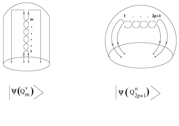
Figure 8: Balls containing the rooms $Q_{m}^{V}$ and $Q_{2p+1}^{H}$.

The results found so far in this section can be used to determine the CS states corresponding to the rooms $Q_{m}^{V}$ and $Q_{2p+1}^{H}$, displayed in figure 8. In general, these states can be given as a linear combination of the elements of the basis $\{|\,\phi_{l}^{(+)}\,>\}$:

$$|\,\psi\,(Q^{V}_{m})\,>\, = \,\sum_{l=0\atop 2l\,\in\,{\rm Z}\kern-3.8pt{\rm Z}\kern 2.0pt}^{2j}\,\mu_{l}(Q^{V}_{m})\,|\,\phi_{l}^{(+)}\,>$$

$$|\,\psi\,(Q^{H}_{2p+1})\,>\, = \,\sum_{l=0\atop 2l\,\in\,{\rm Z}\kern-3.8pt{\rm Z}\kern 2.0pt}^{2j}\,\mu_{l}(Q^{H}_{2p+1})\,|\,\phi_{l}^{(+)}\,>\,\,.$$ (5.27)

Let us now explain how the coefficients in (5.27) can be determined. We are going to consider first the case of $Q_{m}^{V}$. It is clear that $|\,\psi\,(Q^{V}_{m})\,>$ should coincide with $|\,\psi_{m}\,(A_{1})\,>$ when $A_{1}$ is the room of eq. (5.9). This observation immediately implies that:

$$|\,\psi\,(Q^{V}_{m})\,>\,=\,\sum_{l=0\atop 2l\,\in\,{\rm Z}\kern-3.8pt{\rm Z}\kern 2.0pt}^{2j}\,\mu_{l}^{(+)}\,[\,\Lambda_{l,j}^{(+)}(q)\,]^{m}\,|\,\phi_{l}^{(+)}\,>\,\,.$$ (5.28)

and, therefore, $\mu_{l}(Q^{V}_{m})$ can be written as:

$$\mu_{l}(Q^{V}_{m})\,=\,i^{2(l-<l>)}\,\sqrt{\Bigl{[}\,{4l+1\over 2}\,\Bigr{]}_{+}}\,\,\,(\,\Lambda_{l,j}^{(+)}(q)\,)^{m}\,\,.$$ (5.29)

The room $Q_{2p+1}^{H}$ has $2p+1$ half-twists in the first two strands on the left (see figure 8). Therefore, it is more convenient in this case to expand the state $|\,\psi\,(Q^{H}_{2p+1})\,>$ in terms of a basis in which the action of the braiding of the first two strands on the left is diagonal. Let us denote the elements of such a basis by $\,|\,\tilde{\phi}_{l}^{(-)}\,>$. Notice that the two strands which are braided in $Q_{2p+1}^{H}$ are antiparallel and, thus, each half twist will introduce a factor $\Lambda_{l,j}^{(-)}(q)$ multiplying the $l^{{\rm th}}$ eigenvector. Proceeding as before, it is easy to obtain the vector $|\,\psi\,(Q^{H}_{2p+1})\,>$ in terms of the $\,|\,\tilde{\phi}_{l}^{(-)}\,>$’s. One gets:

$$|\,\psi\,(Q^{H}_{2p+1})\,>\,=\,\sum_{l=0\atop 2l\,\in\,{\rm Z}\kern-3.8pt{\rm Z}\kern 2.0pt}^{2j}\,\mu_{l}^{(-)}\,[\,\Lambda_{l,j}^{(-)}(q)\,]^{2p+1}\,|\,\tilde{\phi}_{l}^{(-)}\,>\,\,.$$ (5.30)

The basis $\{|\,\tilde{\phi}_{l}^{(-)}\,>\}$, referring to the first two strands on the left, and the one constituted by the vectors $|\,\phi_{l}^{(+)}\,>$, which are eigenvectors of the braiding operator of the middle two strands, must be linearly related. Let us represent this relation as:

$$|\,\tilde{\phi}_{r}^{(-)}\,>\,=\,\sum_{l=0\atop 2l\,\in\,{\rm Z}\kern-3.8pt{\rm Z}\kern 2.0pt}^{2j}\,a_{rl}\,|\,\phi_{l}^{(+)}\,>\,\,.$$ (5.31)

The matrix $a_{rl}=<\,\phi_{l}^{(+)}|\,\tilde{\phi}_{r}^{(-)}\,>$ is a duality matrix whose explicit expression shall be determined below. Substituting eq. (5.31) in eq. (5.30), one can get the value of the coefficients $\mu_{l}(Q^{H}_{2p+1})$ appearing in eq. (5.27):

$$\mu_{l}(Q^{H}_{2p+1})\,=\,\sum_{r=0\atop 2r\,\in\,{\rm Z}\kern-3.8pt{\rm Z}\kern 2.0pt}^{2j}\,i^{2(r-<r>)}\,\sqrt{\Bigl{[}\,{4r+1\over 2}\,\Bigr{]}_{+}}\,\,\,(\,\Lambda_{r,j}^{(-)}(q)\,)^{2p+1}\,a_{rl}\,\,.$$ (5.32)

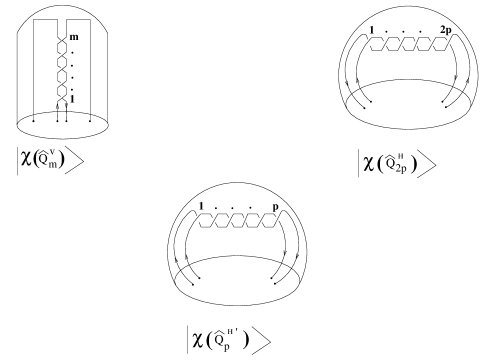
Figure 9: Balls containing the rooms $\hat{Q}^{\,V}_{m}$, $\hat{Q}^{\,H}_{2p}$ and $\hat{Q}^{\,H^{\prime}}_{p}$.

Following the same methods, one can obtain the CS states corresponding to the rooms $\hat{Q}^{\,V}_{m}$, $\hat{Q}^{\,H}_{2p}$ and $\hat{Q}^{\,H^{\prime}}_{p}$ (see figure 9). Let us express them in terms of the basis $\{|\,\phi_{l}^{(-)}\,>\}$, defined in eq. (5.15):

$$|\,\chi\,(\hat{Q}^{\,V}_{m})\,>\, = \,\sum_{l=0\atop 2l\,\in\,{\rm Z}\kern-3.8pt{\rm Z}\kern 2.0pt}^{2j}\,\hat{\mu}_{l}(\hat{Q}^{\,V}_{m})\,|\,\phi_{l}^{(-)}\,>$$

$$|\,\chi\,(\hat{Q}^{\,H}_{2p})\,>\, = \,\sum_{l=0\atop 2l\,\in\,{\rm Z}\kern-3.8pt{\rm Z}\kern 2.0pt}^{2j}\,\hat{\mu}_{l}(\hat{Q}^{\,H}_{2p})\,|\,\phi_{l}^{(-)}\,>$$

$$|\,\chi\,(\hat{Q}^{\,H^{\prime}}_{p})\,>\, = \,\sum_{l=0\atop 2l\,\in\,{\rm Z}\kern-3.8pt{\rm Z}\kern 2.0pt}^{2j}\,\hat{\mu}_{l}(\hat{Q}^{\,H^{\prime}}_{p})\,|\,\phi_{l}^{(-)}\,>\,\,.$$ (5.33)

The coefficients $\hat{\mu}_{l}(\hat{Q}^{\,V}_{m})$, $\hat{\mu}_{l}(\hat{Q}^{\,H}_{2p})$ and $\hat{\mu}_{l}(\hat{Q}^{\,H^{\prime}}_{p})$ entering the linear combinations (5.33) are given by:

$$\hat{\mu}_{l}(\hat{Q}^{\,V}_{m})\, = \,i^{2(l-<l>)}\,\sqrt{\Bigl{[}\,{4l+1\over 2}\,\Bigr{]}_{+}}\,\,\,(\,\Lambda_{l,j}^{(-)}(q)\,)^{m}$$

$$\hat{\mu}_{l}(\hat{Q}^{\,H}_{2p})\, = \,\sum_{r=0\atop 2r\,\in\,{\rm Z}\kern-3.8pt{\rm Z}\kern 2.0pt}^{2j}\,i^{2(r-<r>)}\,\sqrt{\Bigl{[}\,{4r+1\over 2}\,\Bigr{]}_{+}}\,\,\,(\,\Lambda_{r,j}^{(-)}(q)\,)^{2p}\,\,a_{rl}$$

$$\hat{\mu}_{l}(\hat{Q}^{\,H^{\prime}}_{p})\, = \,\sum_{r=0\atop 2r\,\in\,{\rm Z}\kern-3.8pt{\rm Z}\kern 2.0pt}^{2j}\,i^{2(r-<r>)}\,\sqrt{\Bigl{[}\,{4r+1\over 2}\,\Bigr{]}_{+}}\,\,\,(\,\Lambda_{r,j}^{(+)}(q)\,)^{p}\,\,a_{rl}\,\,.$$ (5.34)

The matrix $a_{rl}$ in eq. (5.34) is the same as in eq. (5.32), i.e. is the matrix that relates the braiding in the first two strands to the braiding in the middle two strands. It is clear from its definition that $a_{rl}$ should be related to some of the duality matrices we have found in section 3 for the ${\rm osp}(1|2)$ CFT. There are several non-trivial requirements that $a_{rl}$ must satisfy. These requirements can be obtained as consistency checks of our formalism. Indeed, taking the rooms of figures 8 and 9 as building blocks, one can construct a large variety of knots and links. The polynomial of the knot or link obtained by gluing some of the balls of figures 8 and 9 can be evaluated by substituting eqs. (5.29), (5.32) and (5.34) in eqs. (5.8) and (5.17). In most of the cases there exists more that one way of constructing a given knot or link. This fact can be used to generate many relations which, in particular, allow to determine the matrix $a_{rl}$ uniquely. Let us see some examples. First of all, it is a simple exercise to verify graphically that the link $\hat{L}_{0}(\hat{Q}_{2m}^{H},\hat{Q}_{2p}^{H})$ is the same as $\hat{\cal L}_{2m+2p}$. The equality of the corresponding polynomials requires that:

$$\sum_{{l=0\atop 2l\in{\rm Z}\kern-3.8pt{\rm Z}\kern 2.0pt}}^{2j}\,a_{rl}\,a_{nl}\,=\,\delta_{rn}\,\,.$$ (5.35)

On the other hand, it is obvious that $\hat{L}_{0}(\hat{Q}_{2m}^{H},\hat{Q}_{2p}^{V})$ and $\hat{L}_{0}(\hat{Q}_{2p}^{H},\hat{Q}_{2m}^{H})$ are the same link. However, the corresponding polynomials are equal only if the $a_{rl}$ matrix is symmetric, i.e. if:

$$a_{rl}\,=\,a_{lr}\,\,.$$ (5.36)

Taken together eqs. (5.35) and (5.36) imply that $a_{rl}$ is a symmetric orthogonal matrix. Moreover, it is easy to verify that $\hat{L}_{0}\,(\,\hat{Q}^{\,H}_{2m},\hat{Q}^{\,V}_{0}\,)$ is nothing but the unknot. The requirement:

$$P_{j}[\,\hat{L}_{0}\,(\,\hat{Q}^{\,H}_{2m},\hat{Q}^{\,V}_{0}\,)\,](q)\,=\,P_{j}[\,{\rm unknot}\,](q)\,=\,1\,\,,$$ (5.37)

is fulfilled only if the $a_{rl}$ matrix satisfies:

$$\sum_{l=0\atop 2l\,\in\,{\rm Z}\kern-3.8pt{\rm Z}\kern 2.0pt}^{2j}\,i^{2(l-<l>)}\,\sqrt{\Bigl{[}\,{4l+1\over 2}\,\Bigr{]}_{+}}\,\,\,a_{nl}\,=\,\delta_{n,0}\,\Bigl{[}\,{4j+1\over 2}\,\Bigr{]}_{+}\,\,.$$ (5.38)

It is not difficult to find a solution of eqs. (5.35) , (5.36) and (5.38) in terms of the ${\rm osp}(1|2)$ fusion matrix $F_{rl}^{j}$ of eq. (LABEL:sseis). Actually, one can check that:

$$a_{rl}\,=\,(-1)^{2j}\,F_{rl}^{j}\,\,,$$ (5.39)

satisfies our requirements. Indeed, the symmetry and orthogonality of the matrix (5.39) are a consequence of similar properties of the matrix $F_{rl}^{j}$ (eqs. (B.1) and (B.2)). Moreover, eq. (5.38) is a consequence of eq. (B.4). Other checks of the solution (5.39) for $a_{rl}$, some of them highly non-trivial, are presented in appendix C.

Once the duality matrix $a_{rl}$ is determined, we can evaluate the invariant polynomials for all types of knots and links [16]. The result we get from our building blocks can be simply related to the results found in ref. [16] for the su$(2)$ polynomials. In fact, what we get for arbitrary knots and links is exactly the same relation found in section 4 for torus links (eq. (4.25)). If $P_{j}[L](q)$ ($\tilde{P}_{j}[L](t))$ is the isospin $j$ ${\rm osp}(1|2)$ (su$(2)$) polynomial, in the variable $q$ (respectively, $t$), of the link $L$, one has:

$$P_{j}[L](q)\,=\,(-1)^{2j(\nu_{L}-1)}\,\tilde{P}_{2j}[L](-q)\,\,,$$ (5.40)

where $\nu_{l}$ is the number of components of the link $L$. In order to establish eq. (5.40) in the formalism of this section, one must relate the su$(2)$ and ${\rm osp}(1|2)$ braiding eigenvalues, both for parallel and antiparallel strands. The frame corrected su$(2)$ braiding eigenvalues, which we shall denote by $\tilde{\Lambda}_{l,j}^{+}(t)$ and $\tilde{\Lambda}_{l,j}^{-}(t)$, are well known:

$$\tilde{\Lambda}_{l,j}^{+}(t)\, = \,(-1)^{2j-l}\,t^{2j(j+1)-{l(l+1)\over 2}}$$

$$\tilde{\Lambda}_{l,j}^{-}(t)\, = \,(-1)^{l}\,t^{{l(l+1)\over 2}}$$

$$l\, = \,0,\cdots,2j,\,\,\,\,\,\,\,\,\,\,\,\,\,\,\,\,\,l\in{\rm Z}\kern-3.8pt{\rm Z}\kern 2.0pt\,\,.$$ (5.41)

It is easy to verify that, when $t$ is identified with $-q$, the ${\rm osp}(1|2)$ and su$(2)$ eigenvalues are related as:

$$\Lambda_{l,j}^{+}(q)\, = \,(-1)^{2j}\,\tilde{\Lambda}_{2l,2j}^{+}(-q)$$

$$\Lambda_{l,j}^{-}(q)\, = \,\tilde{\Lambda}_{2l,2j}^{-}(-q)$$

$$l\, = \,0,\cdots,2j,\,\,\,\,\,\,\,\,\,\,\,\,\,\,\,\,\,2l\in{\rm Z}\kern-3.8pt{\rm Z}\kern 2.0pt\,\,.$$ (5.42)

In the process of demonstrating the statement contained in (5.40), it is also necessary to use the relation between the su$(2)$ and ${\rm osp}(1|2)$ CS duality matrices. Let us denote the former by $\tilde{a}_{r,l}(t)$. As proved in ref. [16] $\tilde{a}_{r,l}(t)$ is given by:

$$\tilde{a}_{r,l}(t)\,=\,\tilde{F}_{rl}^{j}(t)\,\,,$$ (5.43)

where $\tilde{F}_{rl}^{j}(t)$ is the su$(2)$ fusion matrix of eq. (3.35). Therefore, as the su$(2)$ and ${\rm osp}(1|2)$ fusion matrices are related as in eq. (3.37), it follows that:

$$a_{rl}\,=\,(-1)^{2j}\,\tilde{a}_{2r,2l}(-q)\,\,.$$ (5.44)

         

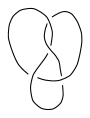
Figure 10: Representation of the figure eight knot.

Using eqs. (5.42), (5.44) and the relation between the su$(2)$ and ${\rm osp}(1|2)$ q-numbers (eq. (2.24)), one can prove eq. (5.10) case by case. The su$(2)$ polynomials for non-trivial knots and links, obtained from four-strand braids, carrying arbitrary isospin representations have been tabulated in ref. [16] and can be compared with our results. In order to illustrate this comparison, we explicitly compute the ${\rm osp}(1|2)$ polynomial for the first simplest knot which is not a torus knot: the figure eight knot. This knot, which in the mathematics literature is usually denoted by $4_{{\scriptstyle 1}}$, has been depicted in figure 10. It is not difficult to verify that the knot of figure 10 can be obtained by gluing together the rooms $\hat{Q}_{2}^{V}$ and $\hat{Q}_{-2}^{H}$. Indeed, the $4_{{\scriptstyle 1}}$ knot is nothing but what we were calling $\hat{L}_{0}(\hat{Q}_{2}^{V},\hat{Q}_{-2}^{H})$ and, thus, we can write:

$$P_{j}[\,4_{{\scriptstyle 1}}\,](q)\,=\,{1\over SD_{q}[j]}\,\sum_{{l=0\atop 2l\in{\rm Z}\kern-3.8pt{\rm Z}\kern 2.0pt}}^{2j}\,\mu_{l}^{(-)}(\hat{Q}_{2}^{V})\,\mu_{l}^{(-)}(\hat{Q}_{-2}^{H})\,\,.$$ (5.45)

Taking the values of $\mu_{l}^{(-)}(\hat{Q}_{2}^{V})$ and $\mu_{l}^{(-)}(\hat{Q}_{-2}^{H})$ from eq. (5.34) and substituting them in the right-hand side of eq. (5.45), one arrives at:

$$P_{j}[\,4_{{\scriptstyle 1}}\,](q)\, = \,{1\over SD_{q}[j]}\,\sum_{{l=0\atop 2l\in{\rm Z}\kern-3.8pt{\rm Z}\kern 2.0pt}}^{2j}\,\sum_{{r=0\atop 2r\in{\rm Z}\kern-3.8pt{\rm Z}\kern 2.0pt}}^{2j}\,i^{2(l-<l>)}\,i^{2(r-<r>)}\,\times$$

$$\times\sqrt{\Bigl{[}\,{4l+1\over 2}\,\Bigr{]}_{+}}\,\sqrt{\Bigl{[}\,{4r+1\over 2}\,\Bigr{]}_{+}}\,a_{lr}\,\Bigl{(}\,\Lambda_{l,j}^{(-)}(q)\,\Bigr{)}^{2}\,\Bigl{(}\,\Lambda_{r,j}^{(-)}(q)\,\Bigr{)}^{-2}\,\,.$$

Moreover, since $SD_{q}[j]=(-1)^{2j}[4j+1]$ when $t=-q$ (see eqs. (2.22) and (2.25)), and making use of eqs. (2.24), (5.42) and (5.44), it is straightforward to verify that eq. (LABEL:ctctres) can be put in the form:

$$P_{j}[\,4_{{\scriptstyle 1}}\,](q)\,=\,{1\over[4j+1]}\,\sum_{{l=0\atop l\in{\rm Z}\kern-3.8pt{\rm Z}\kern 2.0pt}}^{4j}\,\sum_{{r=0\atop r\in{\rm Z}\kern-3.8pt{\rm Z}\kern 2.0pt}}^{4j}\,\sqrt{[\,4l+1\,]}\,\sqrt{[\,4r+1\,]}\,\tilde{a}_{l,r}(-q)\,\Bigl{(}\,\tilde{\Lambda}_{l,2j}^{(-)}(-q)\,\Bigr{)}^{2}\,\Bigl{(}\,\tilde{\Lambda}_{r,2j}^{(-)}(-q)\,\Bigr{)}^{-2}\,\,,$$ (5.47)

which, indeed, shows that $P_{j}[\,4_{{\scriptstyle 1}}\,](q)\,=\,\tilde{P}_{2j}[\,4_{{\scriptstyle 1}}\,](-q)$, in agreement with eq. (5.40).

6 Summary and conclusions

We have studied the behaviour of the conformal blocks under the crossing symmetry operations in osp$(1|2)$ CFT. We have concentrated our efforts in the four-point correlators on the two-sphere. Our main tool has been the Coulomb gas representation of the conformal blocks which is obtained in the free field realization of the osp$(1|2)$ current algebra. We have found closed expressions for the braiding and fusion matrices which, at least for the equal isospin case studied in section 3, are very similar to the ones corresponding to the su$(2)$ CFT.

As mentioned at the end of section 2, the $q=-t$ correspondence between osp$(1|2)$ and su$(2)$ has been previously noticed in the context of the quantum group theory. The fact that our fusion and braiding matrices can also be connected to their su$(2)$ counterparts by means of this identification (see eqs. (3.37) and (3.45)) is an indication of their quantum group origin, i.e. it can be considered as a clue that reveals the existence of a hidden $U_{q}({\rm osp}(1|2))$ symmetry in the model studied. In order to confirm this conclusion, one should verify whether or not the fusion matrix of the osp$(1|2)$ CFT is given by the $6j$ symbols of $U_{q}({\rm osp}(1|2))$. It is interesting to point out in this respect that an analytical expression of the $6j$ symbols of $U_{q}({\rm osp}(1|2))$ has been recently reported in ref. [28]. This expression is very similar to the one we have found for the fusion matrix (eq. (LABEL:sseis)). However, it has been obtained with normalization conventions different from the ones we have adopted here. Therefore, the comparison between the $6j$ symbols of ref. [28] and eq. (LABEL:sseis) cannot be done easily and, as a consequence, more work is required in order to reach a firm conclusion about this subject.

Our analysis of section 4 has served to verify explicitly the connection between the osp$(1|2)$ CS theory and the corresponding CFT. It is interesting to notice that this connection is not exactly the same as in the su$(2)$ case. Indeed, we have found that the osp$(1|2)$ Wilson line operators are not, in general, Verlinde operators (they can differ in a sign, see eq. (4.12)). This difference, which is crucial in order to reproduce the fusion algebra in the space of the characters, could shed light in the analysis of the validity of the Verlinde theorem in other non-unitary CFTs. Notice that one can interpret the sign appearing in the right-hand side of eq. (4.25) as coming from the relative sign between the Verlinde and Wilson line operators in eq. (4.12).

It is also interesting to point out the consistency between the genus one analysis of section 4 and the genus zero formalism of section 5. Actually, both approaches are complementary since the information obtained with the knot operators can be used to fix the parameters of the genus zero formalism. It is interesting to notice the highly non-trivial checks that the duality matrix of eq. (5.31) must satisfy. The fact that we were able to find a consistent solution for this duality matrix (eq. (5.39)) is a new confirmation of the correctness of our ansatz of eq. (LABEL:sseis) for the fusion matrix.

There are, of course, many possible extensions of our work. The most obvious one is the analysis of the invariants corresponding to multicoloured links, i.e. to links with a different osp$(1|2)$ representation in each of their components. This analysis requires to extend our study of the two-dimensional crossing symmetry to a more general class of conformal blocks. It would be interesting to see if there also exists in this case a relation with the su$(2)$ results. On the other hand, this analysis could be the starting point in the formulation of a quantum topology program that could lead to the discovery of new invariants for three-manifolds in the line of ref. [29]. Within the quantum group approach the osp$(1|2)$ invariants for three-manifolds have been considered in ref. [30]. In the CS framework one must compute the vacuum expectation values of tetrahedral configurations of Wilson lines (see the second paper of ref. [6]). The values of this tetrahedra should be related to the $6j$ symbols of $U_{q}({\rm osp}(1|2))$ and, presumably, also to the fusion matrix of our osp$(1|2)$ CFT.

7 Acknowledgements

P. R. would like to thank the Department of Particle Physics of the University of Santiago, where this work was initiated, for hospitality. We would also like to thank J. M. F. Labastida for discussions. This work was supported in part by DGICYT under grant PB93-0344, by CICYT under grant AEN96-1673 and by the European Union TMR grant ERBFMRXCT960012.

APPENDIX A

Let us consider the integrals appearing in the vacuum expectation values of the type (3.10) for $j_{1}=j_{2}=1/2$. In the free field representation described in the main text, these correlators are given by contour integrals that involve the function:

$$\eta(\tau_{1},\tau_{2}) = -\Bigl{\{}\,<\,\chi(0)\,\chi(1))\,(w(\infty))^{1+s}\,w(\tau_{1})\,>\,<\,\psi(\tau_{1})\bar{\psi}(\tau_{2})\,>\,+\,$$ (A.1)

$$+<\,\chi(0)\,\chi(1))\,(w(\infty))^{1+s}\,w(\tau_{2})\,>\,<\,\bar{\psi}(\tau_{1})\psi(\tau_{2})\,>\,\Bigr{\}}\,\,.$$

(Compare eq. (A.1) with eq. (3.13)). The function (A.1) is multiplied in the integrand of the free-field representation of (3.10) by functions of the type:

$$f_{1}(\tau_{1},\tau_{2})\, = \,\tau_{1}^{a}\,\tau_{2}^{a}\,(\tau_{1}-z)^{b}\,(\tau_{2}-z)^{b}\,(\tau_{1}-1)^{b}\,(\tau_{2}-1)^{b}\,(\tau_{1}-\tau_{2})^{2\rho}$$

$$f_{2}(\tau_{1},\tau_{2})\, = \,\tau_{1}^{a}\,\tau_{2}^{a}\,(\tau_{1}-z)^{b}\,(z-\tau_{2})^{b}\,(\tau_{1}-1)^{b}\,(1-\tau_{2})^{b}\,(\tau_{1}-\tau_{2})^{2\rho}$$ (A.2)

$$f_{3}(\tau_{1},\tau_{2})\, = \,\tau_{1}^{a}\,\tau_{2}^{a}\,(z-\tau_{1})^{b}\,(z-\tau_{2})^{b}\,(1-\tau_{1})^{b}\,(1-\tau_{2})^{b}\,(\tau_{1}-\tau_{2})^{2\rho}\,\,.$$

The phases of the functions (A.2) have been chosen in agreement with eq. (LABEL:cuarenta). Let us denote by ${\cal I}_{p}(z)$ the integrals defining the blocks ${}^{s}{\cal F}^{1234}_{p}(z)$. The ${\cal I}_{p}$’s are given by ordered contour integrals (see eq. (3.14)). Closely related to these functions are the integrals:

$$I_{1}(z)\, = \,z^{2\rho}\,(1-z)^{2\rho}\,\int_{1}^{\infty}\,du_{1}\,\int_{1}^{\infty}du_{2}\,f_{1}(u_{1},u_{2})\,\,\eta(u_{1},u_{2})\,$$

$$I_{2}(z)\, = \,z^{2\rho}\,(1-z)^{2\rho}\,\int_{1}^{\infty}\,du_{1}\,\int_{0}^{z}dv_{1}\,\,f_{2}(u_{1},v_{1})\,\eta(u_{1},v_{1})$$ (A.3)

$$I_{3}(z)\, = \,z^{2\rho}\,(1-z)^{2\rho}\,\int_{0}^{z}\,dv_{1}\,\int_{0}^{z}dv_{2}\,f_{3}(v_{1},v_{2})\,\eta(v_{1},v_{2})\,\,.$$

The only difference between the ${\cal I}_{p}$’s and the $I_{p}$’s is the fact that in the former all double integrations in a given interval are ordered, whereas, as shown in eq. (A.3), no such an ordering appears in the expression that defines the $I_{p}$’s. It is easy to prove that these two types of integrals are proportional to each other. In fact one has:

$$I_{1}(z)\, = 2e^{i\pi(\rho-{1\over 2})}\,c(\rho-{1\over 2})\,{\cal I}_{1}(z)$$

$$I_{2}(z)\, = {\cal I}_{2}(z)$$ (A.4)

$$I_{3}(z)\, = 2e^{i\pi(\rho-{1\over 2})}\,c(\rho-{1\over 2})\,{\cal I}_{3}(z)\,\,,$$

where $c(x)\equiv cos\pi x$. It will be convenient in what follows to use the functions $I_{p}(z)$ rather than the ordered integrals ${\cal I}_{p}(z)$. The contours of integration in eq. (A.3) are the ones shown in figure 2 for the particular case $n=2$. Notice that, in order to simplify the notation, we have suppressed the $p$-dependence of the function $\eta_{p}(\{u_{i}\},\{v_{i}\})$ in the right-hand side of eq. (A.3).

In order to obtain the matrix elements of the braiding matrix ${\cal B}^{{1\over 2}}$, one has to relate the integrals ${\cal I}_{p}(z)$ to the $s$-channel blocks corresponding to the correlator:

$${\cal F}^{1324}(z)\,\equiv\,<\,\Phi^{{1\over 2}}_{-{1\over 2}}(0)\,\Phi^{{1\over 2}}_{-{1\over 2}}(1)\,\Phi^{{1\over 2}}_{{1\over 2}}(z)\,\tilde{\Phi}^{{1\over 2}}_{{1\over 2}}(\infty)\,Q^{2}\,>\,.$$ (A.5)

         

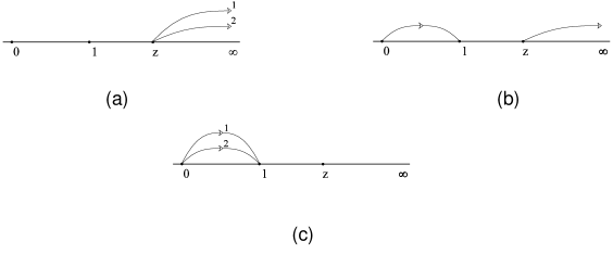
Figure 11: Contours of integration used in the definition of ${\cal J}_{p}(z)$ and $J_{p}(z)$ for $p=1$(a), $p=2$(b) and $p=3$(c).

The integral appearing in the free field representation of the block ${}^{s}{\cal F}^{1324}_{p}(z)$ will be denoted by ${\cal J}_{p}(z)$. In this case, the contours of integration differ from the ones of figure 2 in the exchange of the points $\tau=1$ and $\tau=z$. The contours corresponding to the s-channel intermediate states of the correlator (A.5) are shown in figure 11. As in the case of figure 2, the integrals along the contours of figure 11 can be ordered or not. The ordered ones are those appearing in the free field blocks, i.e. in the ${\cal J}_{p}$’s, while the integrals that are not ordered will be denoted by $J_{p}(z)$. The actual expressions of the latter are:

$$J_{1}(z)\, = \,z^{2\rho}\,(z-1)^{2\rho}\,\int_{z}^{\infty}\,du_{1}\,\int_{z}^{\infty}du_{2}\,f_{1}(u_{1},u_{2})\,\eta(u_{1},u_{2})\,$$

$$J_{2}(z)\, = \,z^{2\rho}\,(z-1)^{2\rho}\,\int_{z}^{\infty}\,du_{1}\,\int_{0}^{1}dv_{1}\,f_{2}(u_{1},v_{1})\,\eta(u_{1},v_{1})$$ (A.6)

$$J_{3}(z)\, = \,z^{2\rho}\,(z-1)^{2\rho}\,\int_{0}^{1}\,dv_{1}\,\int_{0}^{1}dv_{2}\,f_{3}(v_{1},v_{2})\,\eta(v_{1},v_{2})\,\,.$$

The relation between the $J_{p}$ and ${\cal J}_{p}$ integrals is similar to the one written in eq. (A.4), namely:

$$J_{1}(z)\, = 2e^{i\pi(\rho-{1\over 2})}\,c(\rho-{1\over 2})\,{\cal J}_{1}(z)$$

$$J_{2}(z)\, = {\cal J}_{2}(z)$$ (A.7)

$$J_{3}(z)\, = 2e^{i\pi(\rho-{1\over 2})}\,c(\rho-{1\over 2})\,{\cal J}_{3}(z)\,\,.$$

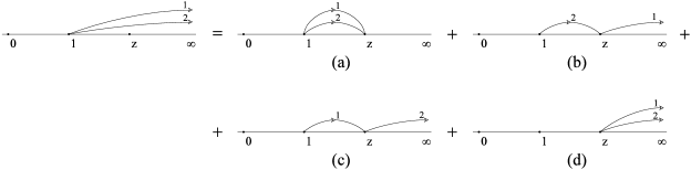
Figure 12: Decomposition of $I_{1}(z)$ for $z>1$ into a sum of integrals in the intervals $(1,z)$ and $(z,\infty)$.

The phase convention used to define the integrals $I_{p}(z)$ and ${\cal I}_{p}(z)$ corresponds to the situation in which $z<1$, which is the ordering of these two points in the contours of figure 2. On the contrary, as shown in figure 11, one should define the integrals $J_{p}(z)$ and ${\cal J}_{p}(z)$ with a phase convention adapted to the ordering in which $z$ is greater than one. In order to relate the integrals ${\cal I}_{p}(z)$ and ${\cal J}_{p}(z)$ one must, first of all, analytically continue the ${\cal I}_{p}(z)$’s to the region $z>1$. After this is done, these two integrals are related linearly as follows:

$${\cal I}_{p}(z)\,=\,\sum_{l=1}^{3}\,c_{pl}\,{\cal J}_{l}(z)\,\,.$$ (A.8)

Taking into account the definitions of the functions ${\cal I}_{p}(z)$ and ${\cal J}_{p}(z)$ and of the braiding matrix (eq. (3.3)), it is clear that:

$${\cal B}^{{1\over 2}}_{j_{p}\,j_{l}}\,=\,c_{pl}\,\,,$$ (A.9)

where the relation between the isospin and the number of contours is given in eq. (3.16).

As mentioned above, in order to obtain the explicit value of the coefficients $c_{pl}$, it is more convenient to deal with the integrals (A.3) and (A.6). The relation between these two types of integrals can be obtained by using contour manipulation techniques [17]. We shall illustrate this procedure by showing in detail how the $I_{1}(z)$ integral can be put in terms of $J_{1}(z)$, $J_{2}(z)$ and $J_{3}(z)$. First of all, one must assume that in $I_{1}(z)$, the variable $z$ is analytically continued to the region $z>1$. The function $I_{1}(z)$ is defined by means of a double integration in the interval $(1,\infty)$. As shown in figure 12, each of these two integrals in the interval $(1,\infty)$ can be represented as the sum of two integrals performed along the $(1,z)$ and $(z,\infty)$ intervals. One gets in this way four contributions of the type:

$$I_{1}(z)\,=\,I_{1}^{(a)}(z)\,+\,I_{1}^{(b)}(z)\,+\,I_{1}^{(c)}(z)\,+\,I_{1}^{(d)}(z)\,\,,$$ (A.10)

where the superindices $a$, $b$, $c$ and $d$ refer to the four contributions displayed in figure 12. In all the integrals of the right-hand side of eq. (A.10), the integrand is the same as in $I_{1}(z)$. It is clear by inspection that the integral $I_{1}^{(d)}(z)$ is of the same type of $J_{1}(z)$ (see figure 11a). Taking into account the different conventions for the relative phase of $z$ and $1$, one can write:

$$I_{1}^{(d)}(z)\,=\,e^{2i\pi\rho}\,J_{1}(z)\,\,.$$ (A.11)

The other three remaining integrals are defined along contours that do not correspond to any of those shown in figure 11. It is in these cases where the manipulation of contours is needed. Let us explain in detail this technique for the integral $I_{1}^{(b)}$. In this case, the variable which is not integrated over the intervals represented in figure 11 (i.e. $(0,1)$ and $(z,\infty)$) is the one we have called $2$. This variable is integrated in $I_{1}^{(b)}$ over the interval $(1,z)$. By “opening” the contour, one can convert this integral into an integral in which the variable $2$ runs over the intervals $(\infty,1)$ and $(z,\infty)$. One must, however, be careful with the phases that are picked up when the branch points of the integrand are crossed. In fact, we have two different possibilities to open the contour of the variable $2$. If we open the contour from above, we get the following representation of $I_{1}^{(b)}$:

(A.12)

while, on the contrary, opening the contour of the variable 2 from below, we obtain:

(A.13)

In eqs. (A.12) and (A.13) the left-hand side is the same. The first two integrals of the right-hand side of these equations correspond to some of the contours of figure 11, whereas the third term does not coincide with any of the integration paths that define the functions $J_{p}(z)$. In order to get rid of this unwanted integral, we shall multiply eq. (A.12) by $e^{-i\pi(a+b)}$ and let us subtract it from the result of multiplying eq. (A.13) by $e^{i\pi(a+b)}$. After these manipulations, one can obtain $I_{1}^{(b)}(z)$ in terms of $J_{1}(z)$ and $J_{2}(z)$. This result is the following:

$$I_{1}^{(b)}(z)\,=\,-e^{i\pi(b+\rho+{1\over 2})}\,\,{s(a+2b+\rho-{1\over 2})\over s(a+b)}\,\,J_{1}(z)\,-\,e^{i\pi(b+2\rho)}\,\,{s(a)\over s(a+b)}\,\,J_{2}(z)\,\,,$$ (A.14)

where $s(x)\equiv sin\pi x$. The other contributions appearing in the right-hand side of eq. (A.10) can be treated similarly. For the integral $I_{1}^{(a)}(z)$ one gets:

$$I_{1}^{(a)}(z) = e^{2i\pi(b+\rho)}\,\,{s(a+2b+2\rho-1)\,s(a+2b+\rho-{1\over 2})\over s(a+b)\,s(a+b+\rho-{1\over 2})}\,\,J_{1}(z)\,+$$

$$+\,e^{i\pi(2b+3\rho-{1\over 2})}\,\,{s(a)\,s(a+2b+2\rho-1)\over s(a+b+\rho-{1\over 2})}\,\Biggl{[}\,{1\over s(a+b)}\,+\,{1\over s(a+b+2\rho-1)}\,\Biggr{]}\,J_{2}(z)\,+$$

$$+\,e^{2i\pi(b+\rho)}\,\,{s(a)\,s(a+\rho-{1\over 2})\over s(a+b+\rho-{1\over 2})\,s(a+b+2\rho-1)}\,J_{3}(z)\,\,,$$

while $I_{1}^{(c)}(z)$ can be written as:

$$I_{1}^{(c)}(z)\,=\,-e^{i\pi(b+3\rho-{1\over 2})}\,\,{s(a+2b+\rho-{1\over 2})\over s(a+b)}\,\,J_{1}(z)\,-\,e^{i\pi(b+4\rho-1)}\,\,{s(a)\over s(a+b)}\,\,J_{2}(z)\,\,.$$ (A.16)

Putting together the results of eqs. (A.11), (A.14), (LABEL:apaquince) and (A.16), and taking into account the relation with the ordered integrals (eqs. (A.4) and (A.7)), one obtains the following values for the matrix elements $c_{1l}$:

$$c_{11} = e^{2i\pi(a+2b+2\rho-{1\over 2})}\,\,{s(b)\,s(b+\rho-{1\over 2})\over s(a+b+\rho-{1\over 2})\,s(a+b)}$$

$$c_{12} = e^{i\pi(a+3b+4\rho-1)}\,\,{s(a)\,s(b)\over s(a+b+2\rho-1)\,s(a+b)}$$ (A.17)

$$c_{13} = e^{2i\pi(b+\rho)}\,\,{s(a)\,s(a+\rho-{1\over 2})\over s(a+b+\rho-{1\over 2})\,s(a+b+2\rho-1)}\,\,.$$

Using these techniques, although in some cases the calculations are much more involved, the other elements of the braiding matrix can be obtained. The result is:

$$c_{21} = 2\,e^{i\pi(a+3b+4\rho-1)}\,\,\,{s(a+2b+\rho-{1\over 2})\,s(b+\rho-{1\over 2})\,\,c(\rho-{1\over 2})\over s(a+b)\,s(a+b+\rho-{1\over 2})}$$

$$c_{22} = e^{i\pi(2b+4\rho-1)}\,\,\,{s(a)\,s(a+2b+2\rho-1)\,-\,[s(b)]^{2}\over s(a+b)\,s(a+b+2\rho-1)}$$

$$c_{23} = -2\,e^{i\pi(b-a+2\rho)}\,\,\,{s(b+\rho-{1\over 2})\,s(a+\rho-{1\over 2})\,\,\,c(\rho-{1\over 2})\over s(a+b+\rho-{1\over 2})\,s(a+b+2\rho-1)}$$ (A.18)

$$c_{31} = e^{2i\pi(b+\rho)}\,\,\,{s(a+2b+2\rho-1)\,s(a+2b+\rho-{1\over 2})\over s(a+b)\,s(a+b+\rho-{1\over 2})}$$

$$c_{32} = -\,e^{i\pi(b-a+2\rho)}\,\,\,{s(a+2b+2\rho-1)\,s(b)\over s(a+b)\,s(a+b+2\rho-1)}$$

$$c_{33} = e^{-2i\pi(a-{1\over 2})}\,\,\,{s(b+\rho-{1\over 2})\,s(b)\over s(a+b+\rho-{1\over 2})\,s(a+b+2\rho-1)}\,\,.$$

Substituting $a=b=-\alpha_{0}^{2}=-2\rho$ in eqs. (A.17) and (A.18), and taking eq. (A.9) into account, one arrives at the matrix ${\cal B}^{{1\over 2}}$ of eq. (3.30).

APPENDIX B

In this appendix we shall collect some properties of the duality matrix $F^{j}$. Some of these properties can be obtained directly from eq. (LABEL:sseis), while others can be easily derived from the identification (3.37) between the ${\rm osp}(1|2)$ and su$(2)$ fusion matrices.

It is evident after inspecting eq. (LABEL:sseis) that $F^{j}$ is a symmetric matrix, namely one has:

$$F_{j_{1}\,j_{2}}^{j}\,=F_{j_{2}\,j_{1}}^{j}\,\,.$$ (B.1)

Moreover, $F^{j}$ is an orthogonal matrix, i.e. it satisfies:

$$\sum_{j_{3}}\,F_{j_{1}\,j_{3}}^{j}\,\,F_{j_{2}\,j_{3}}^{j}\,=\,\delta_{j_{1},j_{2}}\,\,.$$ (B.2)

By means of a direct substitution in eq. (LABEL:sseis), one can obtain the value of the first row (or column):

$$F_{0\,j_{1}}^{j}\,=\,(-1)^{2j}\,\,i^{\,2(j_{1}-<j_{1}>)}\,\,\,{\sqrt{\Bigl{[}\,{4j_{1}+1\over 2}\Bigr{]}_{+}}\over\Bigl{[}\,{4j+1\over 2}\Bigr{]}_{+}}\,\,.$$ (B.3)

Substituting the above value in the orthogonality condition (eq. (B.2)), one gets:

$$\sum_{j_{2}}\,i^{\,2(j_{2}-<j_{2}>)}\,\,\sqrt{\Bigl{[}\,{4j_{2}+1\over 2}\Bigr{]}_{+}}\,\,F_{j_{1}\,j_{2}}^{j}\,=\,(-1)^{2j}\,\Bigl{[}\,{4j+1\over 2}\Bigr{]}_{+}\,\,\delta_{j_{1},0}\,\,.$$ (B.4)

Let the Casimir of the isospin $j$ representation be defined as in the main text, namely $c_{j}\,=\,j\,(\,j+{1\over 2}\,)$. The fusion matrix also satisfies:

$$\sum_{j_{3}}\,(-1)^{<j_{3}>}\,\,q^{\pm 2c_{j_{3}}\mp 8c_{j}}\,\,F_{j_{3}\,j_{1}}^{j}\,F_{j_{3}\,j_{2}}^{j}\,=\,(-1)^{<j_{1}>+<j_{2}>}\,q^{\mp 2c_{j_{1}}\mp 2c_{j_{2}}}\,\,F_{j_{1}\,j_{2}}^{j}(q)\,\,.$$ (B.5)

Eq. (B.5) can be proved from a similar relation verified by the su$(2)$ fusion matrix. In particular, taking $j_{2}=0$ and using the value of $F_{0\,j_{1}}^{j}$, one arrives at:

$$\sum_{j_{3}}\,(-1)^{<j_{3}>}\,\,i^{\,2(j_{3}-<j_{3}>)}\,\,q^{\pm 2c_{j_{3}}\mp 8c_{j}}\,\,\sqrt{\Bigl{[}\,{4j_{3}+1\over 2}\Bigr{]}_{+}}\,F_{j_{3}\,j_{1}}^{j}\,=\,$$

$$=\,(-1)^{<j_{1}>}\,\,q^{\mp 2c_{j_{1}}}\,\,i^{\,2(j_{1}-<j_{1}>)}\,\,\sqrt{\Bigl{[}\,{4j_{1}+1\over 2}\Bigr{]}_{+}}\,\,.$$ (B.6)

APPENDIX C

In this appendix we verify that our solution (5.39) for the CS duality matrix satisfies several consistency relations, which constitutes a confirmation of the correctness of our result (5.39) for $a_{rl}$. The relations we are going to check can be obtained by following the same procedure as the one used in ref. [16] for the su$(2)$ case. Some of the possible checks are satisfied as a consequence of the orthogonality and symmetry properties of the $a_{rl}$ matrix. For example, the link $L_{0}(Q_{2p+1}^{H},Q_{2m+1}^{H})$ is the same as the link $\hat{\cal L}_{2p+2m+2}$. It is easy to prove that the corresponding polynomials are the same if the matrix $a_{rl}$ is orthogonal. The verification of other consistency conditions requires the use of more specific properties of the ${\rm osp}(1|2)$ fusion matrix, such as the ones listed in appendix B. So, for instance, as:

$$L_{0}(\,Q_{1}^{H},Q_{m}^{V}\,)\,=\,{\cal L}_{m+1}\,\,,$$ (C.1)

one must have:

$$\sum_{l,r=0\atop 2l,2r\,\in\,{\rm Z}\kern-3.8pt{\rm Z}\kern 2.0pt}^{2j}\,\,i^{2(r-<r>)}\,i^{2(l-<l>)}\,\sqrt{\Bigl{[}\,{4r+1\over 2}\,\Bigr{]}_{+}}\,\,\,\sqrt{\Bigl{[}\,{4l+1\over 2}\,\Bigr{]}_{+}}\,\,\,\Lambda_{r,j}^{(-)}(q)\,\,(\,\Lambda_{l,j}^{(+)}(q)\,)^{m}\,a_{rl}\,=\,$$

$$=\,\sum_{l=0\atop 2l\,\in\,{\rm Z}\kern-3.8pt{\rm Z}\kern 2.0pt}^{2j}\,\,(-1)^{2l}\,\Bigl{[}\,{4l+1\over 2}\,\Bigr{]}_{+}\,\,(\,\Lambda_{l,j}^{(+)}(q)\,)^{m+1}\,\,.$$ (C.2)

Let us prove that the matrix (5.39) satisfies eq. (C.2). If we substitute $\Lambda_{r,j}^{(-)}(q)\,=\,(-1)^{<r>}\,q^{2c_{r}}$ and $a_{rl}\,=\,(-1)^{2j}\,F_{rl}^{j}$ in the left-hand side of eq. (C.2), the sum in $r$ can be evaluated with the help of eq. (B.6):

$$\sum_{r=0\atop 2r\,\in\,{\rm Z}\kern-3.8pt{\rm Z}\kern 2.0pt}^{2j}\,\,(-1)^{<r>}\,i^{2(r-<r>)}\,\sqrt{\Bigl{[}\,{4r+1\over 2}\,\Bigr{]}_{+}}\,\,\,\,q^{2c_{r}}\,\,a_{rl}\,=\,$$

$$=\,(-1)^{2j+<l>}\,q^{8c_{j}-2c_{l}}\,i^{2(l-<l>)}\,\sqrt{\Bigl{[}\,{4l+1\over 2}\,\Bigr{]}_{+}}\,=$$

$$=\,\Lambda_{l,j}^{(+)}(q)\,i^{2(l-<l>)}\,\sqrt{\Bigl{[}\,{4l+1\over 2}\,\Bigr{]}_{+}}\,\,,$$ (C.3)

where, in the last step, we have taken into account that $\Lambda_{l,j}^{(+)}(q)\,=\,(-1)^{2j+<l>}\,q^{8c_{j}-2c_{l}}$. Using this result in the left-hand side of eq. (C.2), one verifies the consistency required.

Another non-trivial check of our solution for the CS duality matrix has its origin in the link equivalence:

$$L_{0}(\,Q_{2p+1}^{H},Q_{1}^{V}\,)\,=\,\hat{\cal L}_{2p+2}\,\,,$$ (C.4)

which implies the following equation for $a_{rl}$:

$$\sum_{l,r=0\atop 2l,2r\,\in\,{\rm Z}\kern-3.8pt{\rm Z}\kern 2.0pt}^{2j}\,\,i^{2(r-<r>)}\,i^{2(l-<l>)}\,\sqrt{\Bigl{[}\,{4r+1\over 2}\,\Bigr{]}_{+}}\,\,\,\sqrt{\Bigl{[}\,{4l+1\over 2}\,\Bigr{]}_{+}}\,\,\,(\,\Lambda_{r,j}^{(-)}(q)\,)^{2p+1}\,\,\Lambda_{l,j}^{(+)}(q)\,\,\,a_{rl}\,=\,$$

$$=\,\sum_{r=0\atop 2r\,\in\,{\rm Z}\kern-3.8pt{\rm Z}\kern 2.0pt}^{2j}\,\,(-1)^{2r}\,\Bigl{[}\,{4r+1\over 2}\,\Bigr{]}_{+}\,\,(\,\Lambda_{r,j}^{(-)}(q)\,)^{2p+2}\,\,.$$ (C.5)

Taking $a_{rl}\,=\,(-1)^{2j}\,F_{rl}^{j}$ and $\Lambda_{l,j}^{(+)}(q)\,=\,(-1)^{2j+<l>}\,q^{8c_{j}-2c_{l}}\,\,$, and using again eq. (B.6), the sum in $l$ in the left-hand side of eq. (C.5) can be performed:

$$\sum_{l=0\atop 2l\,\in\,{\rm Z}\kern-3.8pt{\rm Z}\kern 2.0pt}^{2j}\,\,(-1)^{<l>}\,i^{2(l-<l>)}\, q^{8c_{j}-2c_{l}}\,\sqrt{\Bigl{[}\,{4l+1\over 2}\,\Bigr{]}_{+}}\,\,\,F_{rl}^{j}\,=\,(-1)^{<r>}\,q^{2c_{r}}\,\,i^{2(r-<r>)}\,\sqrt{\Bigl{[}\,{4r+1\over 2}\,\Bigr{]}_{+}}\,=\,$$ (C.6)

$$=\,i^{2(r-<r>)}\,\Lambda_{r,j}^{(-)}(q)\,\sqrt{\Bigl{[}\,{4r+1\over 2}\,\Bigr{]}_{+}}\,\,,$$

and, as a consequence, eq. (C.5) is satisfied by the CS duality matrix (5.39).

References

[1] G. Moore and N. Seiberg, Phys. Lett.B212 (1988) 451; Commun. Math. Phys.123 (1989) 177.
[2] For a review see J. Fuchs, “Affine Lie algebras and quantum groups”, (Cambridge
University Press, Cambridge, 1992), S. Ketov, “Conformal Field Theory”, (World Scientific,
Singapore, 1995) and C. Gomez, M. Ruiz-Altaba and G.
Sierra, “Quantum groups in two-dimensional
physics”, (Cambridge University Press, Cambridge, 1996).
[3] L. Alvarez-Gaumé, C. Gomez and G. Sierra,
Phys. Lett.B220 (1989) 142;
Nucl. Phys.B319 (1989) 155;
Nucl. Phys.B330 (1990) 347.
[4] A. N. Kirillov and N. Yu. Reshetikhin,
“ Representation of the algebra ,q-orthogonal polynomials and invariants of links”, in
“Infinite dimensional Lie algebras and groups”,
ed. V. G. Kac (World Scientific, Singapore, 1989).
[5] N. Yu. Reshetikhin, “Quantized universal
enveloping algebras and invariants of links I, II”,
LOMI preprints E-4-87 and E-17-87.
[7]M. Bershadsky and H.
Ooguri, Phys. Lett.B229 (1989) 374.
[8]A. M. Polyakov and A. B.
Zamolodchikov, Mod. Phys. Lett.A3 (1988) 1213.
[9] I. P. Ennes, A. V. Ramallo and J. M. Sanchez
de Santos, Phys. Lett.B389 (1996) 485;
Nucl. Phys.B491 [PM] (1997) 574.
[10] J. H. Horne, Nucl. Phys.B334 (1990)
669.
[11] L. H. Kauffman and H. Saleur,
Commun. Math. Phys.141 (1991) 293;
Int. J. Mod. Phys.A7 (1992) 493.
[12] L. Rozansky and H. Saleur,
Nucl. Phys.B376 (1992) 461.
[13]
T. Deguchi, J. Phys. Soc. Jap.58 (1989) 3441;
T. Deguchi and Y. Akutsu,
J. Phys.A: Math. Gen.23
(1990) 1861.
[14]
R. B. Zhang, M. D. Gould and A. J. Bracken,
Commun. Math. Phys.137 (1991) 13;
R. B. Zhang, J. Math. Phys.32 (1991) 2605;
R. B. Zhang, J. Math. Phys.33 (1992) 3918;
J. R. Links, M. D. Gould and R. B. Zhang,
Rev. Math. Phys.5 (1993) 345;
M. D. Gould, I. Tshohantjis and A. J. Bracken,
Rev. Math. Phys.5 (1993) 533;
J. R. Links and R. B. Zhang,
J. Math. Phys.35 (1994) 1377.
[15] J.M.F. Labastida and A.V. Ramallo,
Phys. Lett.B227 (1989) 92;
Phys. Lett.B228 (1989) 214;
J.M.F. Labastida, P. M. Llatas and A.V. Ramallo,
Nucl. Phys.B348 (1991) 651.
[16] R.K. Kaul and T.R. Govindarajan,
Nucl. Phys.B380 (1992) 293;
Nucl. Phys.B393 (1993) 392;
P. Ramadevi, T. R. Govindarajan and R.K. Kaul,
Nucl. Phys.B402 (1993) 548;
R. K. Kaul, Commun. Math. Phys.162 (1994) 289.
[17] Vl.S.Dotsenko and V. A. Fateev,
Nucl. Phys.B240 (1984) 312;
Nucl. Phys.B251 (1985) 691; Phys. Lett.B154
(1985) 291.
[18] E. Verlinde,
Nucl. Phys.B300 (1988) 360.
[19]A. Pais and V.
Rittenberg, J. Math. Phys.16 (1975) 2063; M.
Scheunert, W. Nahn and V.
Rittenberg, J. Math. Phys.18 (1977) 155.
[20]J. B. Fan and M. Yu, “Modules over
affine Lie superalgebras” , Academia Sinica preprint
AS-ITP-93-14, hep-th/9304122.
[21] R. Dijkgraaf and E. Verlinde,
Nucl. Phys. (Proc. Suppl. )5B (1988) 87.
[22]P. Kulish and N.
Reshetikhin, Lett. Math. Phys.18 (1989) 143.
[23] H. Saleur,
Nucl. Phys.B336 (1990) 363.
[24] See, for example, L. H. Kauffman,
“Knots and Physics” (World Scientific, Singapore,
1991).
[26] Y. Akutsu and M. Wadati,
J. Phys. Soc. Jap.56 (1987) 839; Y. Akutsu, T. Deguchi and M.
Wadati, J. Phys. Soc. Jap.56 (1987) 3464;
J. Phys. Soc. Jap.57 (1988) 757; for a review see
M. Wadati, T. Deguchi and Y. Akutsu,
Phys. Rep.180 (1989) 247.
[27] W.B.R. Lickorish and K.C. Millet, Topology26 (1987) 107.
[28] P. Minnaert and M. Mozrzymas,
J. Math. Phys.38 (1997) 2676.
[29] V. Turaev and O. Viro,
Topology31 (1992) 865;
N. Reshetikin and V. Turaev,
Invent. Math.103 (1991) 547;
L. H. Kauffman and S. Lins,
“ Temperley-Lieb recoupling
theory and invariants of 3-manifolds”, Annals of Math.
Studies vol. 134, ( Princeton University Press, Princeton,
1994).