CERN-TH/97-218

hep-th/9709062

INTRODUCTION TO SUPERSTRING THEORY

Elias Kiritsis Theory Division, CERN,
CH-1211, Geneva 23, SWITZERLAND

In these lecture notes, an introduction to superstring theory is presented. Classical strings, covariant and light-cone quantization, supersymmetric strings, anomaly cancelation, compactification, T-duality, supersymmetry breaking, and threshold corrections to low-energy couplings are discussed. A brief introduction to non-perturbative duality symmetries is also included.

Lectures presented at the Catholic University of Leuven and

at the University of Padova during the academic year 1996-97.

To be published by Leuven University Press.

CERN-TH/97-218

March 1997

1 Introduction

String theory has been the leading candidate over the past years for a theory that consistently unifies all fundamental forces of nature, including gravity. In a sense, the theory predicts gravity and gauge symmetry around flat space. Moreover, the theory is UV-finite. The elementary objects are one-dimensional strings whose vibration modes should correspond to the usual elementary particles.

At distances large with respect to the size of the strings, the low-energy excitations can be described by an effective field theory. Thus, contact can be established with quantum field theory, which turned out to be successful in describing the dynamics of the real world at low energy.

I will try to explain here the basic structure of string theory, its predictions and problems.

In chapter 2 the evolution of string theory is traced, from a theory initially built to describe hadrons to a “theory of everything”. In chapter 3 a description of classical bosonic string theory is given. The oscillation modes of the string are described, preparing the scene for quantization. In chapter 4, the quantization of the bosonic string is described. All three different quantization procedures are presented to varying depth, since in each one some specific properties are more transparent than in others. I thus describe the old covariant quantization, the light-cone quantization and the modern path-integral quantization. In chapter 6 a concise introduction is given, to the central concepts of conformal field theory since it is the basic tool in discussing first quantized string theory. In chapter 8 the calculation of scattering amplitudes is described. In chapter 9 the low-energy effective action for the massless modes is described.

In chapter 10 superstrings are introduced. They provide spacetime fermions and realize supersymmetry in spacetime and on the world-sheet. I go through quantization again, and describe the different supersymmetric string theories in ten dimensions. In chapter 11 gauge and gravitational anomalies are discussed. In particular it is shown that the superstring theories are anomaly-free. In chapter 12 compactifications of the ten-dimensional superstring theories are described. Supersymmetry breaking is also discussed in this context. In chapter 13, I describe how to calculate loop corrections to effective coupling constants. This is very important for comparing string theory predictions at low energy with the real world. In chapter 14 a brief introduction to non-perturbative string connections and non-perturbative effects is given. This is a fast-changing subject and I have just included some basics as well as tools, so that the reader orients him(her)self in the web of duality connections. Finally, in chapter 15 a brief outlook and future problems are presented.

I have added a number of appendices to make several technical discussions self-contained. In Appendix A useful information on the elliptic $\vartheta$-functions is included. In Appendix B, I rederive the various lattice sums that appear in toroidal compactifications. In Appendix C the Kaluza-Klein ansatz is described, used to obtain actions in lower dimensions after toroidal compactification. In Appendix D some facts are presented about four-dimensional locally supersymmetric theories with N=1,2,4 supersymmetry. In Appendix E, BPS states are described along with their representation theory and helicity supertrace formulae that can be used to trace their appearance in a supersymmetric theory. In Appendix F facts about elliptic modular forms are presented, which are useful in many contexts, notably in the one-loop computation of thresholds and counting of BPS multiplicities. In Appendix G, I present the computation of helicity-generating string partition functions and the associated calculation of BPS multiplicities. Finally, in Appendix H, I briefly review electric–magnetic duality in four dimensions.

I have not tried to be complete in my referencing. The focus was to provide, in most cases, appropriate reviews for further reading. Only in the last chapter, which covers very recent topics, I do mostly refer to original papers because of the scarcity of relevant reviews.

2 Historical perspective

In the sixties, physicists tried to make sense of a big bulk of experimental data relevant to the strong interaction. There were lots of particles (or “resonances”) and the situation could best be described as chaotic. There were some regularities observed, though:

$\bullet$ Almost linear Regge behavior. It was noticed that the large number of resonances could be nicely put on (almost) straight lines by plotting their mass versus their spin

$$m^{2}={J\over\alpha^{\prime}}\;,$$ (2.1)

with $\alpha^{\prime}\sim 1$ GeV^-2, and this relation was checked up to $J=11/2$.

$\bullet$ s-t duality. If we consider a scattering amplitude of two$\to$ two hadrons ($1,2\to 3,4$), then it can be described by the Mandelstam invariants

$$s=-(p_{1}+p_{2})^{2}\;\;\;,\;\;\;t=-(p_{2}+p_{3})^{2}\;\;\;,\;\;\;u=-(p_{1}+p_{3})^{2}\;,$$ (2.2)

with $s+t+u=\sum_{i}m_{i}^{2}$. We are using a metric with signature $(-+++)$. Such an amplitude depends on the flavor quantum numbers of hadrons (for example SU(3)). Consider the flavor part, which is cyclically symmetric in flavor space. For the full amplitude to be symmetric, it must also be cyclically symmetric in the momenta $p_{i}$. This symmetry amounts to the interchange $t\leftrightarrow s$. Thus, the amplitude should satisfy $A(s,t)=A(t,s)$. Consider a $t$-channel contribution due to the exchange of a spin-$J$ particle of mass $M$. Then, at high energy

$$A_{J}(s,t)\sim{(-s)^{J}\over t-M^{2}}\,.$$ (2.3)

Thus, this partial amplitude increases with $s$ and its behavior becomes worse for large values of $J$. If one sews amplitudes of this form together to make a loop amplitude, then there are uncontrollable UV divergences for $J>1$. Any finite sum of amplitudes of the form (2.3) has this bad UV behavior. However, if one allows an infinite number of terms then it is conceivable that the UV behavior might be different. Moreover such a finite sum has no $s$-channel poles.

A proposal for such a dual amplitude was made by Veneziano [1]

$$A(s,t)={\Gamma(-\alpha(s))\Gamma(-\alpha(t))\over\Gamma(-\alpha(s)-\alpha(t))}\,,$$ (2.4)

where $\Gamma$ is the standard $\Gamma$-function and

$$\alpha(s)=\alpha(0)+\alpha^{\prime}s\,.$$ (2.5)

By using the standard properties of the $\Gamma$-function it can be checked that the amplitude (2.4) has an infinite number of $s,t$-channel poles:

$$A(s,t)=-\sum_{n=0}^{\infty}{(\alpha(s)+1)\dots(\alpha(s)+n)\over n!}{1\over\alpha(t)-n}\,.$$ (2.6)

In this expansion the $s\leftrightarrow t$ interchange symmetry of (2.4) is not manifest. The poles in (2.6) correspond to the exchange of an infinite number of particles of mass $M^{2}=(n-\alpha(0)/\alpha^{\prime})$ and high spins. It can also be checked that the high-energy behavior of the Veneziano amplitude is softer than any local quantum field theory amplitude, and the infinite number of poles is crucial for this.

It was subsequently realized by Nambu and Goto that such amplitudes came out of theories of relativistic strings. However such theories had several shortcomings in explaining the dynamics of strong interactions.

$\bullet$ All of them seemed to predict a tachyon.

$\bullet$ Several of them seemed to contain a massless spin-2 particle that was impossible to get rid of.

$\bullet$ All of them seemed to require a spacetime dimension of 26 in order not to break Lorentz invariance at the quantum level.

$\bullet$ They contained only bosons.

At the same time, experimental data from SLAC showed that at even higher energies hadrons have a point-like structure; this opened the way for quantum chromodynamics as the correct theory that describes strong interactions.

However some work continued in the context of “dual models” and in the mid-seventies several interesting breakthroughs were made.

$\bullet$ It was understood by Neveu, Schwarz and Ramond how to include spacetime fermions in string theory.

$\bullet$ It was also understood by Gliozzi, Scherk and Olive how to get rid of the omnipresent tachyon. In the process, the constructed theory had spacetime supersymmetry.

$\bullet$ Scherk and Schwarz, and independently Yoneya, proposed that closed string theory, always having a massless spin-2 particle, naturally describes gravity and that the scale $\alpha^{\prime}$ should be identified with the Planck scale. Moreover, the theory can be defined in four dimensions using the Kaluza–Klein idea, namely considering the extra dimensions to be compact and small.

However, the new big impetus for string theory came in 1984. After a general analysis of gauge and gravitational anomalies [2], it was realized that anomaly-free theories in higher dimensions are very restricted. Green and Schwarz showed in [3] that open superstrings in 10 dimensions are anomaly-free if the gauge group is O(32). $\rm E_{8}\times E_{8}$ was also anomaly-free but could not appear in open string theory. In [4] it was shown that another string exists in ten dimensions, a hybrid of the superstring and the bosonic string, which can realize the E${}_{8}\times$E₈ or O(32) gauge symmetry.

Since the early eighties, the field of string theory has been continuously developing and we will see the main points in the rest of these lectures. The reader is encouraged to look at a more detailed discussion in [5]–[8].

One may wonder what makes string theory so special. One of its key ingredients is that it provides a finite theory of quantum gravity, at least in perturbation theory. To appreciate the difficulties with the quantization of Einstein gravity, we will look at a single-graviton exchange between two particles (Fig. 1a). We will set $h=c=1$. Then the amplitude is proportional to $E^{2}/M_{\rm Planck}^{2}$, where $E$ is the energy of the process and $M_{\rm Planck}$ is the Planck mass, $M_{\rm Planck}\sim 10^{19}~{}$GeV. It is related to the Newton constant $G_{N}\sim M_{\rm Planck}^{2}$. Thus, we see that the gravitational interaction is irrelevant in the IR ($E<<M_{\rm Planck}$) but strongly relevant in the UV. In particular it implies that the two-graviton exchange diagram (Fig. 1b) is proportional to

$${1\over M_{\rm Planck}^{4}}\int_{0}^{\Lambda}dE~{}E^{3}\sim{\Lambda^{4}\over M_{\rm Planck}^{4}}\,,$$ (2.7)

which is strongly UV-divergent. In fact it is known that Einstein gravity coupled to matter is non-renormalizable in perturbation theory. Supersymmetry makes the UV divergence softer but the non-renormalizability persists.

Figure 1: Gravitational interaction between two particles via graviton exchange.

There are two ways out of this:

$\bullet$ There is a non-trivial UV fixed-point that governs the UV behavior of quantum gravity. To date, nobody has managed to make sense out of this possibility.

$\bullet$ There is new physics at $E\sim M_{\rm Planck}$ and Einstein gravity is the IR limit of a more general theory, valid at and beyond the Planck scale. You could consider the analogous situation with the Fermi theory of weak interactions. There, one had a non-renormalizable current–current interaction with similar problems, but today we know that this is the IR limit of the standard weak interaction mediated by the $W^{\pm}$ and $Z^{0}$ gauge bosons. So far, there is no consistent field theory that can make sense at energies beyond $M_{\rm Planck}$ and contains gravity. Strings provide precisely a theory that induces new physics at the Planck scale due to the infinite tower of string excitations with masses of the order of the Planck mass and carefully tuned interactions that become soft at short distance.

Moreover string theory seems to have all the right properties for Grand Unification, since it produces and unifies with gravity not only gauge couplings but also Yukawa couplings. The shortcomings, to date, of string theory as an ideal unifying theory are its numerous different vacua, the fact that there are three string theories in 10 dimensions that look different (type-I, type II and heterotic), and most importantly supersymmetry breaking. There has been some progress recently in these directions: there is good evidence that these different-looking string theories might be non-perturbatively equivalent.

3 Classical string theory

As in field theory there are two approaches to discuss classical and quantum string theory. One is the first quantized approach, which discusses the dynamics of a single string. The dynamical variables are the spacetime coordinates of the string. This is an approach that is forced to be on-shell. The other is the second-quantized or field theory approach. Here the dynamical variables are functionals of the string coordinates, or string fields, and we can have an off-shell formulation. Unfortunately, although there is an elegant formulation of open string field theory, the closed string field theory approaches are complicated and difficult to use. Moreover the open theory is not complete since we know it also requires the presence of closed strings. In these lectures we will follow the first-quantized approach, although the reader is invited to study the rather elegant formulation of open string field theory [11].

3.1 The point particle

Before discussing strings, it is useful to look first at the relativistic point particle. We will use the first-quantized path integral language. Point particles classically follow an extremal path when traveling from one point in spacetime to another. The natural action is proportional to the length of the world-line between some initial and final points:

$$S=m\int^{s_{f}}_{s_{i}}ds=m\int^{\tau_{1}}_{\tau_{0}}d\tau\sqrt{-\eta_{\mu\nu}\dot{x}^{\mu}\dot{x}^{\nu}},$$ (3.1.1)

where $\eta_{\mu\nu}=\mbox{diag}(-1,+1,+1,+1)$. The momentum conjugate to $x^{\mu}(\tau)$ is

$$p_{\mu}=-\frac{\delta L}{\delta\dot{x}^{\mu}}=\frac{m\dot{x}_{\mu}}{\sqrt{-\dot{x}^{2}}},$$ (3.1.2)

and the Lagrange equations coming from varying the action (3.1.1) with respect to $X^{\mu}(\tau)$ read

$$\partial_{\tau}\left(\frac{m\dot{x}_{\mu}}{\sqrt{-\dot{x}^{2}}}\right)=0.$$ (3.1.3)

Equation (3.1.2) gives the following mass-shell constraint :

$$p^{2}+m^{2}=0.$$ (3.1.4)

The canonical Hamiltonian is given by

$$H_{can}=\frac{\partial L}{\partial\dot{x}^{\mu}}\dot{x}^{\mu}-L.$$ (3.1.5)

Inserting (3.1.2) into (3.1.5) we can see that $H_{can}$ vanishes identically. Thus, the constraint (3.1.4) completely governs the dynamics of the system. We can add it to the Hamiltonian using a Lagrange multiplier. The system will then be described by

$$H=\frac{N}{2m}(p^{2}+m^{2}),$$ (3.1.6)

from which it follows that

$$\dot{x}^{\mu}=\{x^{\mu},H\}=\frac{N}{m}p^{\mu}=\frac{N\dot{x}^{\mu}}{\sqrt{-\dot{x}^{2}}},$$ (3.1.7)

or

$$\dot{x}^{2}=-N^{2},$$ (3.1.8)

so we are describing time-like trajectories. The choice N=1 corresponds to a choice of scale for the parameter $\tau$, the proper time.

The square root in (3.1.1) is an unwanted feature. Of course for the free particle it is not a problem, but as we will see later it will be a problem for the string case. Also the action we used above is ill-defined for massless particles. Classically, there exists an alternative action, which does not contain the square root and in addition allows the generalization to the massless case. Consider the following action :

$$S=-{\textstyle{1\over 2}}\int d\tau e(\tau)\left(e^{-2}(\tau)(\dot{x}^{\mu})^{2}-m^{2}\right).$$ (3.1.9)

The auxiliary variable $e(\tau)$ can be viewed as an einbein on the world-line. The associated metric would be $g_{\tau\tau}=e^{2}$, and (3.1.9) could be rewritten as

$$S=-{\textstyle{1\over 2}}\int d\tau\sqrt{\mbox{det}g_{\tau\tau}}(g^{\tau\tau}\partial_{\tau}x\cdot\partial_{\tau}x-m^{2}).$$ (3.1.10)

The action is invariant under reparametrizations of the world-line. An infinitesimal reparametrization is given by

$$\delta x^{\mu}(\tau)=x^{\mu}(\tau+\xi(\tau))-x^{\mu}(\tau)=\xi(\tau)\dot{x}^{\mu}+{\cal{O}}(\xi^{2}).$$ (3.1.11)

Varying $e$ in (3.1.9) leads to

$$\delta S={\textstyle{1\over 2}}\int d\tau\left(\frac{1}{e^{2}(\tau)}(\dot{x}^{\mu})^{2}+m^{2}\right)\delta e(\tau).$$ (3.1.12)

Setting $\delta S=0$ gives us the equation of motion for $e$ :

$$e^{-2}x^{2}+m^{2}=0\;\;\;\to\;\;\;e=\frac{1}{m}\sqrt{-\dot{x}^{2}}\;.$$ (3.1.13)

Varying $x$ gives

$$\delta S={\textstyle{1\over 2}}\int d\tau e(\tau)\left(e^{-2}(\tau)2\dot{x}^{\mu}\right)\partial_{\tau}\delta x^{\mu}.$$ (3.1.14)

After partial integration, we find the equation of motion

$$\partial_{\tau}(e^{-1}\dot{x}^{\mu})=0.$$ (3.1.15)

Substituting (3.1.13) into (3.1.15), we find the same equations as before (cf. eq. (3.1.3)). If we substitute (3.1.13) directly into the action (3.1.9), we find the previous one, which establishes the classical equivalence of both actions.

We will derive the propagator for the point particle. By definition,

$$\langle x|x^{\prime}\rangle=N\int_{x(0)=x}^{x(1)=x^{\prime}}DeDx^{\mu}\mbox{exp}\left({1\over 2}\int_{0}^{1}\left(\frac{1}{e}(\dot{x}^{\mu})^{2}-em^{2}\right)d\tau\right),$$ (3.1.16)

where we have put $\tau_{0}=0$, $\tau_{1}=1$.

Under reparametrizations of the world-line, the einbein transforms as a vector. To first order, this means

$$\delta e=\partial_{\tau}(\xi e).$$ (3.1.17)

This is the local reparametrization invariance of the path. Since we are integrating over $e$, this means that (3.1.16) will give an infinite result. Thus, we need to gauge-fix the reparametrization invariance (3.1.17). We can gauge-fix $e$ to be constant. However, (3.1.17) now indicates that we cannot fix more. To see what this constant may be, notice that the length of the path of the particle is

$$L=\int_{0}^{1}d\tau\sqrt{\mbox{det}g_{\tau\tau}}=\int_{0}^{1}d\tau e,$$ (3.1.18)

so the best we can do is $e=L$. This is the simplest example of leftover (Teichmüller) parameters after gauge fixing. The $e$ integration contains an integral over the constant mode as well as the rest. The rest is the “gauge volume” and we will throw it away. Also, to make the path integral converge, we rotate to Euclidean time $\tau\to i\tau$. Thus, we are left with

$$\langle x|x^{\prime}\rangle=N\int_{0}^{\infty}dL\int_{x(0)=x}^{x(1)=x^{\prime}}Dx^{\mu}\mbox{exp}\left(-{1\over 2}\int_{0}^{1}\left(\frac{1}{L}\dot{x}^{2}+Lm^{2}\right)d\tau\right).$$ (3.1.19)

Now write

$$x^{\mu}(\tau)=x^{\mu}+(x^{\prime\mu}-x^{\mu})\tau+\delta x^{\mu}(\tau),$$ (3.1.20)

where $\delta x^{\mu}(0)=\delta x^{\mu}(1)=0$. The first two terms in this expansion represent the classical path. The measure for the fluctuations $\delta x^{\mu}$ is

$$\parallel\delta x\parallel^{2}=\int_{0}^{1}d\tau e(\delta x^{\mu})^{2}=L\int_{0}^{1}d\tau(\delta x^{\mu})^{2},$$ (3.1.21)

so that

$$Dx^{\mu}\sim\prod_{\tau}\sqrt{L}d\delta x^{\mu}(\tau).$$ (3.1.22)

Then

$$\langle x|x^{\prime}\rangle=N\int_{0}^{\infty}dL\int\prod_{\tau}\sqrt{L}d\delta x^{\mu}(\tau)e^{-\frac{(x^{\prime}-x)^{2}}{2L}-m^{2}L/2}e^{-\frac{1}{2L}\int_{0}^{1}(\delta\dot{x^{\mu}})^{2}}.$$ (3.1.23)

The Gaussian integral involving $\delta\dot{x}^{\mu}$ can be evaluated immediately :

$$\int\prod_{\tau}\sqrt{L}d\delta x^{\mu}(\tau)e^{-\frac{1}{L}\int_{0}^{1}(\delta\dot{x^{\mu}})^{2}}\sim\left(\mbox{det}\left(-\frac{1}{L}\partial^{2}_{\tau}\right)\right)^{-\frac{D}{2}}.$$ (3.1.24)

We have to compute the determinant of the operator $-\partial^{2}_{\tau}/L$. To do this we will calculate first its eigenvalues. Then the determinant will be given as the product of all the eigenvalues. To find the eigenvalues we consider the eigenvalue problem

$$-{1\over L}\partial^{2}_{\tau}\psi(\tau)=\lambda\psi(\tau)$$ (3.1.25)

with the boundary conditions $\psi(0)=\psi(1)=0$. Note that there is no zero mode problem here because of the boundary conditions. The solution is

$$\psi_{n}(\tau)=C_{n}\sin(n\pi\tau)\;\;\;,\;\;\;\lambda_{n}={n^{2}\over L}\;\;\;,\;\;\;n=1,2,\ldots$$ (3.1.26)

and thus

$$\mbox{det}\left(-\frac{1}{L}\partial^{2}_{\tau}\right)=\prod_{n=1}^{\infty}{n^{2}\over L}\,.$$ (3.1.27)

Obviously the determinant is infinite and we have to regularize it. We will use $\zeta$-function regularization in which

$$\prod_{n=1}^{\infty}L^{-1}=L^{-\zeta(0)}=L^{1/2}\;\;\;,\;\;\;\prod_{n=1}^{\infty}n^{a}=e^{-a\zeta^{\prime}(0)}=(2\pi)^{a/2}\,.$$ (3.1.28)

Adjusting the normalization factor we finally obtain

$$\langle x|x^{\prime}\rangle={1\over 2(2\pi)^{D/2}}\int_{0}^{\infty}dLL^{-\frac{D}{2}}e^{-\frac{(x^{\prime}-x)^{2}}{2L}-m^{2}L/2}=$$ (3.1.29)

$$={1\over(2\pi)^{D/2}}\left({|x-x^{\prime}|\over m}\right)^{(2-D)/2}K_{(D-2)/2}(m|x-x^{\prime}|).$$

This is the free propagator of a scalar particle in D dimensions. To obtain the more familiar expression, we have to pass to momentum space

$$|p\rangle=\int d^{D}xe^{ip\cdot x}|x\rangle\,,$$ (3.1.30)

$$\langle p|p^{\prime}\rangle = \int d^{D}xe^{-ip\cdot x}\int d^{D}x^{\prime}~{}e^{ip^{\prime}\cdot x^{\prime}}\langle x|x^{\prime}\rangle$$

$$= {1\over 2}\int d^{D}x^{\prime}e^{i(p^{\prime}-p)\cdot x^{\prime}}\int_{0}^{\infty}dL~{}e^{-{L\over 2}(p^{2}+m^{2})}$$

$$= (2\pi)^{D}\delta(p-p^{\prime})~{}\frac{1}{p^{2}+m^{2}},$$

just as expected.

Here we should make one more comment. The momentum space amplitude $\langle p|p^{\prime}\rangle$ can also be computed directly if we insert in the path integral $e^{ip\cdot x}$ for the initial state and $e^{-ip^{\prime}\cdot x}$ for the final state. Thus, amplitudes are given by path-integral averages of the quantum-mechanical wave-functions of free particles.

3.2 Relativistic strings

We now use the ideas of the previous section to construct actions for strings. In the case of point particles, the action was proportional to the length of the world-line between some initial point and final point. For strings, it will be related to the surface area of the “world-sheet” swept by the string as it propagates through spacetime. The Nambu-Goto action is defined as

$$S_{NG}=-T\int dA.$$ (3.2.1)

The constant factor $T$ makes the action dimensionless; its dimensions must be $[\mbox{length}]^{-2}$ or $[\mbox{mass}]^{2}$. Suppose $\xi^{i}$ ($i=0,1$) are coordinates on the world-sheet and $G_{\mu\nu}$ is the metric of the spacetime in which the string propagates. Then, $G_{\mu\nu}$ induces a metric on the world-sheet :

$$ds^{2}=G_{\mu\nu}(X)dX^{\mu}dX^{\nu}=G_{\mu\nu}\frac{\partial X^{\mu}}{\partial\xi^{i}}\frac{\partial X^{\nu}}{\partial\xi^{j}}d\xi^{i}d\xi^{j}=G_{ij}d\xi^{i}d\xi^{j}\,,$$ (3.2.2)

where the induced metric is

$$G_{ij}=G_{\mu\nu}\partial_{i}X^{\mu}\partial_{j}X^{\nu}.$$ (3.2.3)

This metric can be used to calculate the surface area. If the spacetime is flat Minkowski space then $G_{\mu\nu}=\eta_{\mu\nu}$ and the Nambu-Goto action becomes

$$S_{NG}=-T\int\sqrt{-\mbox{det}G_{ij}}d^{2}\xi=-T\int\sqrt{(\dot{X}.X^{\prime})^{2}-(\dot{X}^{2})(X^{\prime 2})}d^{2}\xi,$$ (3.2.4)

where $\dot{X}^{\mu}=\frac{\partial X^{\mu}}{\partial\tau}$ and $X^{\prime\mu}=\frac{\partial X^{\mu}}{\partial\sigma}$ ($\tau=\xi^{0}$, $\sigma=\xi^{1}$ ). The equations of motion are

$$\partial_{\tau}\left(\frac{\delta L}{\delta\dot{X}^{\mu}}\right)+\partial_{\sigma}\left(\frac{\delta L}{\delta X^{\prime\mu}}\right)=0.$$ (3.2.5)

Depending on the kind of strings, we can impose different boundary conditions. In the case of closed strings, the world-sheet is a tube. If we let $\sigma$ run from $0$ to $\bar{\sigma}=2\pi$, the boundary condition is periodicity

$$X^{\mu}(\sigma+\bar{\sigma})=X^{\mu}(\sigma).$$ (3.2.6)

For open strings, the world-sheet is a strip, and in this case we will put $\bar{\sigma}=\pi$. Two kinds of boundary conditions are frequently used :

• Neumann :

  $$\left.\frac{\delta L}{\delta X^{\prime\mu}}\right|_{\sigma=0,\bar{\sigma}}=0;$$ (3.2.7)

• Dirichlet :

  $$\left.\frac{\delta L}{\delta\dot{X}^{\mu}}\right|_{\sigma=0,\bar{\sigma}}=0.$$ (3.2.8)

As we shall see at the end of this section, Neumann conditions imply that no momentum flows off the ends of the string. The Dirichlet condition implies that the end-points of the string are fixed in spacetime. We will not discuss them further, but they are relevant for describing (extended) solitons in string theory also known as D-branes [10].

The momentum conjugate to $X^{\mu}$ is

$$\Pi^{\mu}=\frac{\delta L}{\delta\dot{X}^{\mu}}=-T\frac{(\dot{X}\cdot X^{\prime})X^{\prime\mu}-(X^{\prime})^{2}\dot{X}^{\mu}}{[(X^{\prime}\cdot\dot{X})^{2}-(\dot{X})^{2}(X^{\prime})^{2}]^{1/2}}.$$ (3.2.9)

The matrix $\frac{\delta^{2}L}{\delta\dot{X}^{\mu}\delta\dot{X}^{\nu}}$ has two zero eigenvalues, with eigenvectors $\dot{X}^{\mu}$ and $X^{\prime\mu}$. This signals the occurrence of two constraints that follow directly from the definition of the conjugate momenta. They are

$$\Pi\cdot X^{\prime}=0\;\;\;,\;\;\;\Pi^{2}+T^{2}X^{\prime 2}=0\,.$$ (3.2.10)

The canonical Hamiltonian

$$H=\int_{0}^{\bar{\sigma}}d\sigma(\dot{X}\cdot\Pi-L)$$ (3.2.11)

vanishes identically, just in the case of the point particle. Again, the dynamics is governed solely by the constraints.

The square root in the Nambu-Goto action makes the treatment of the quantum theory quite complicated. Again, we can simplify the action by introducing an intrinsic fluctuating metric on the world-sheet. In this way, we obtain the Polyakov action for strings moving in flat spacetime [12]

$$S_{P}=-{T\over 2}\int d^{2}\xi\sqrt{-\mbox{det}g}~{}g^{\alpha\beta}\partial_{\alpha}X^{\mu}\partial_{\beta}X^{\nu}\eta_{\mu\nu}.$$ (3.2.12)

As is well known from field theory, varying the action with respect to the metric yields the stress-tensor :

$$T_{\alpha\beta}\equiv-\frac{2}{T}\frac{1}{\sqrt{-\mbox{det}g}}\frac{\delta S_{P}}{\delta g^{\alpha\beta}}=\partial_{\alpha}X\cdot\partial_{\beta}X-{\textstyle{1\over 2}}g_{\alpha\beta}g^{\gamma\delta}\partial_{\gamma}X\cdot\partial_{\delta}X.$$ (3.2.13)

Setting this variation to zero and solving for $g_{\alpha\beta}$, we obtain, up to a factor,

$$g_{\alpha\beta}=\partial_{\alpha}X\cdot\partial_{\beta}X.$$ (3.2.14)

In other words, the world-sheet metric $g_{\alpha\beta}$ is classically equal to the induced metric. If we substitute this back into the action, we find the Nambu-Goto action. So both actions are equivalent, at least classically. Whether this is also true quantum-mechanically is not clear in general. However, they can be shown to be equivalent in the critical dimension. From now on we will take the Polyakov approach to the quantization of string theory.

By varying (3.2.12) with respect to $X^{\mu}$, we obtain the equations of motion:

$$\frac{1}{\sqrt{-\mbox{det}g}}\partial_{\alpha}(\sqrt{-\mbox{det}g}g^{\alpha\beta}\partial_{\beta}X^{\mu})=0.$$ (3.2.15)

Thus, the world-sheet action in the Polyakov approach consists of D two-dimensional scalar fields $X^{\mu}$ coupled to the dynamical two-dimensional metric and we are thus considering a theory of two-dimensional quantum gravity coupled to matter. One could ask whether there are other terms that can be added to (3.2.12). It turns out that there are only two: the cosmological term

$$\lambda_{1}\int\sqrt{-\mbox{det}g}$$ (3.2.16)

and the Gauss-Bonnet term

$$\lambda_{2}\int\sqrt{-\mbox{det}g}R^{(2)},$$ (3.2.17)

where $R^{(2)}$ is the two-dimensional scalar curvature associated with $g_{\alpha\beta}$. This gives the Euler number of the world-sheet, which is a topological invariant. So this term cannot influence the local dynamics of the string, but it will give factors that weight various topologies differently. It is not difficult to prove that (3.2.16) has to be zero classically. In fact the classical equations of motion for $\lambda_{1}\not=0$ imply that $g_{\alpha\beta}=0$, which gives trivial dynamics. We will not consider it further. For the open string, there are other possible terms, which are defined on the boundary of the world-sheet.

We will discuss the symmetries of the Polyakov action:

• Poincaré invariance :

  $$\delta X^{\mu}=\omega^{\mu}_{\nu}X^{\nu}+\alpha^{\mu}\;\;\;,\;\;\;\delta g_{\alpha\beta}=0\;,$$ (3.2.18)

  where $\omega_{\mu\nu}=-\omega_{\nu\mu}$;

• local two-dimensional reparametrization invariance :

  $$\delta g_{\alpha\beta} = \xi^{\gamma}\partial_{\gamma}g_{\alpha\beta}+\partial_{\alpha}\xi^{\gamma}g_{\beta\gamma}+\partial_{\beta}\xi^{\gamma}g_{\alpha\gamma}=\nabla_{\alpha}\xi_{\beta}+\nabla_{\beta}\xi_{\alpha},$$

  $$\delta X^{\mu} = \xi^{\alpha}\partial_{\alpha}X^{\mu},$$

  $$\delta(\sqrt{-\mbox{det}g}) = \partial_{\alpha}(\xi^{\alpha}\sqrt{-\mbox{det}g});$$ (3.2.19)

• conformal (or Weyl) invariance :

  $$\delta X^{\mu}=0\;\;\;,\;\;\;\delta g_{\alpha\beta}=2\Lambda g_{\alpha\beta}.$$ (3.2.20)

Due to the conformal invariance, the stress-tensor will be traceless. This is in fact true in general. Consider an action $S(g_{\alpha\beta},\phi^{i})$ in arbitrary spacetime dimensions. We assume that it is invariant under conformal transformations

$$\delta g_{\alpha\beta}=2\Lambda(x)g_{\alpha\beta}\;\;\;,\;\;\;\delta\phi^{i}=d_{i}\Lambda(x)\phi^{i}\;.$$ (3.2.21)

The variation of the action under infinitesimal conformal transformations is

$$0=\delta S=\int d^{2}\xi\left[2\frac{\delta S}{\delta g^{\alpha\beta}}g^{\alpha\beta}+\sum_{i}d_{i}\frac{\delta S}{\delta\phi_{i}}\phi_{i}\right]\Lambda.$$ (3.2.22)

Using the equations of motion for the fields $\phi_{i}$, i.e. $\frac{\delta S}{\delta\phi_{i}}=0$, we find

$$T^{\alpha}_{\alpha}\sim\frac{\delta S}{\delta g^{\alpha\beta}}g^{\alpha\beta}=0\;,$$ (3.2.23)

which follows without the use of the equations of motion, if and only if $d_{i}=0$. This is the case for the bosonic string, described by the Polyakov action, but not for fermionic extensions.

Just as we could fix $e(\tau)$ for the point particle using reparametrization invariance, we can reduce $g_{\alpha\beta}$ to $\eta_{\alpha\beta}=\mbox{diag}(-1,+1)$. This is called conformal gauge. First, we choose a parametrization that makes the metric conformally flat, i.e.

$$g_{\alpha\beta}=e^{2\Lambda(\xi)}\eta_{\alpha\beta}.$$ (3.2.24)

It can be proven that in two dimensions, this is always possible for world-sheets with trivial topology. We will discuss the subtle issues that appear for non-trivial topologies later on.

Using the conformal symmetry, we can further reduce the metric to $\eta_{\alpha\beta}$. We also work with “light-cone coordinates”

$$\xi_{+}=\tau+\sigma\;\;\;,\;\;\;\xi_{-}=\tau-\sigma.$$ (3.2.25)

The metric becomes

$$ds^{2}=-d\xi_{+}d\xi_{-}.$$ (3.2.26)

The components of the metric are

$$g_{++}=g_{--}=0\;\;\;,\;\;\;g_{+-}=g_{-+}=-{1\over 2}$$ (3.2.27)

and

$$\partial_{\pm}={1\over 2}(\partial_{\tau}\pm\partial_{\sigma})\;.$$ (3.2.28)

The Polyakov action in conformal gauge is

$$S_{P}\sim T\int d^{2}\xi~{}\partial_{+}X^{\mu}\partial_{-}X^{\nu}\eta_{\mu\nu}.$$ (3.2.29)

By going to conformal gauge, we have not completely fixed all reparametrizations. In particular, the reparametrizations

$$\xi_{+}\longrightarrow f(\xi_{+})\;\;\;,\;\;\;\xi_{-}\longrightarrow g(\xi_{-})$$ (3.2.30)

only put a factor $\partial_{+}f\partial_{-}g$ in front of the metric, so they can be compensated by the transformation of $d^{2}\xi$.

Notice that here we have exactly enough symmetry to completely fix the metric. A metric on a d-dimensional world-sheet has d(d+1)/2 independent components. Using reparametrizations, d of them can be fixed. Conformal invariance fixes one more component. The number of remaining components is

$$\frac{d(d+1)}{2}-d-1.$$ (3.2.31)

This is zero in the case $d=2$ (strings), but not for $d>2$ (membranes). This makes an analogous treatment of higher-dimensional extended objects problematic.

We will derive the equations of motion from the Polyakov action in conformal gauge (eq. (3.2.29)). By varying $X^{\mu}$, we get (after partial integration):

$$\delta S=T\int d^{2}\xi(\delta X^{\mu}\partial_{+}\partial_{-}X_{\mu})-T\int_{\tau_{0}}^{\tau_{1}}d\tau X^{\prime}_{\mu}\delta X^{\mu}.$$ (3.2.32)

Using periodic boundary conditions for the closed string and

$$\left.X^{\prime\mu}\right|_{\sigma=0,\bar{\sigma}}=0$$ (3.2.33)

for the open string, we find the equations of motion

$$\partial_{+}\partial_{-}X^{\mu}=0.$$ (3.2.34)

Even after gauge fixing, the equations of motion for the metric have to be imposed. They are

$$T_{\alpha\beta}=0,$$ (3.2.35)

or

$$T_{10}=T_{01}={\textstyle{1\over 2}}\dot{X}\cdot X^{\prime}=0\;\;\;,\;\;\;T_{00}=T_{11}=\frac{1}{4}(\dot{X}^{2}+X^{\prime 2})=0,$$ (3.2.36)

which can also be written as

$$(\dot{X}\pm X^{\prime})^{2}=0.$$ (3.2.37)

These are known as the Virasoro constraints. They are the analog of the Gauss law in the string case.

In light-cone coordinates, the components of the stress-tensor are

$$T_{++}={\textstyle{1\over 2}}\partial_{+}X\cdot\partial_{+}X\;\;\;,\;\;\;T_{--}={\textstyle{1\over 2}}\partial_{-}X\cdot\partial_{-}X\;\;\;,\;\;\;T_{+-}=T_{-+}=0.$$ (3.2.38)

This last expression is equivalent to $T^{\alpha}_{\alpha}=0$; it is trivially satisfied. Energy-momentum conservation, $\nabla^{\alpha}T_{\alpha\beta}=0$, becomes

$$\partial_{-}T_{++}+\partial_{+}T_{-+}=\partial_{+}T_{--}+\partial_{-}T_{+-}=0.$$ (3.2.39)

Using (3.2.38), this states

$$\partial_{-}T_{++}=\partial_{+}T_{--}=0\;$$ (3.2.40)

which leads to conserved charges

$$Q_{f}=\int_{0}^{\bar{\sigma}}f(\xi^{+})T_{++}(\xi^{+}),$$ (3.2.41)

and likewise for $T_{--}$. To convince ourselves that $Q_{f}$ is indeed conserved, we need to calculate

$$0=\int d\sigma\partial_{-}(f(\xi^{+})T_{++})=\partial_{\tau}Q_{f}+\left.f(\xi^{+})T_{++}\right|^{\bar{\sigma}}_{0}.$$ (3.2.42)

For closed strings, the boundary term vanishes automatically; for open strings, we need to use the constraints. Of course, there are other conserved charges in the theory, namely those associated with Poincaré invariance :

$$P^{\alpha}_{\mu}=-T\sqrt{\mbox{det}g}g^{\alpha\beta}\partial_{\beta}X_{\mu}\,,$$ (3.2.43)

$$J^{\alpha}_{\mu\nu}=-T\sqrt{\mbox{det}g}g^{\alpha\beta}(X_{\mu}\partial_{\beta}X_{\nu}-X_{\nu}\partial_{\beta}X_{\mu}).$$ (3.2.44)

We have $\partial_{\alpha}P^{\alpha}_{\mu}=0=\partial_{\alpha}J^{\alpha}_{\mu\nu}$ because of the equation of motion for $X$. The associated charges are

$$P_{\mu}=\int_{0}^{\bar{\sigma}}d\sigma P^{\tau}_{\mu}\;\;\;,\;\;\;J_{\mu\nu}=\int_{0}^{\bar{\sigma}}d\sigma J^{\tau}_{\mu\nu}.$$ (3.2.45)

These are conserved, e.g.

$$\frac{\partial P_{\mu}}{\partial\tau} = T\int_{0}^{\bar{\sigma}}d\sigma\partial_{\tau}^{2}X_{\mu}=T\int_{0}^{\bar{\sigma}}d\sigma\partial_{\sigma}^{2}X_{\mu}$$ (3.2.46)

$$= T(\partial_{\sigma}X_{\mu}(\sigma=\bar{\sigma})-\partial_{\sigma}X_{\mu}(\sigma=0)).$$

(In the second line we used the equation of motion for $X$.) This expression automatically vanishes for the closed string. For open strings, we need Neumann boundary conditions. Here we see that these conditions imply that there is no momentum flow off the ends of the string. The same applies to angular momentum.

3.3 Oscillator expansions

We will now solve the equations of motion for the bosonic string,

$$\partial_{+}\partial_{-}X^{\mu}=0\;,$$ (3.3.1)

taking into account the proper boundary conditions. To do this we have to treat the open and closed string cases separately. We will first consider the case of the closed string.

• $\@@underline{\hbox{Closed Strings }}$

  The most general solution to equation (3.3.1) that also satisfies the periodicity condition

  $$X^{\mu}(\tau,\sigma+2\pi)=X^{\mu}(\tau,\sigma)$$

  can be separated in a left- and a right-moving part:

  $$X^{\mu}(\tau,\sigma)=X^{\mu}_{L}(\tau+\sigma)+X^{\mu}_{R}(\tau-\sigma),$$ (3.3.2)

  where

  $$X^{\mu}_{L}(\tau+\sigma)=\frac{x^{\mu}}{2}+\frac{p^{\mu}}{4\pi T}(\tau+\sigma)+\frac{i}{\sqrt{4\pi T}}\sum_{k\neq 0}\frac{\bar{\alpha}^{\mu}_{k}}{k}e^{-ik(\tau+\sigma)},$$

  (3.3.3)

  $$X^{\mu}_{R}(\tau-\sigma)=\frac{x^{\mu}}{2}+\frac{p^{\mu}}{4\pi T}(\tau-\sigma)+\frac{i}{\sqrt{4\pi T}}\sum_{k\neq 0}\frac{\alpha^{\mu}_{k}}{k}e^{-ik(\tau-\sigma)}.$$

  The $\alpha^{\mu}_{k}$ and $\bar{\alpha}^{\mu}_{k}$ are arbitrary Fourier modes, and $k$ runs over the integers. The function $X^{\mu}(\tau,\sigma)$ must be real, so we know that $x^{\mu}$ and $p^{\mu}$ must also be real and we can derive the following reality condition for the $\alpha$’s:

  $$(\alpha^{\mu}_{k})^{*}=\alpha^{\mu}_{-k}\quad\quad\mbox{and}\quad\quad(\bar{\alpha}^{\mu}_{k})^{*}=\bar{\alpha}^{\mu}_{-k}$$ (3.3.4)

  If we define $\alpha^{\mu}_{0}=\bar{\alpha}^{\mu}_{0}=\frac{1}{\sqrt{4\pi T}}p^{\mu}$ we can write

  $$\partial_{-}X^{\mu}_{R}=\frac{1}{\sqrt{4\pi T}}\sum_{k\in\hbox{\mybb Z}}\alpha^{\mu}_{k}e^{-ik(\tau-\sigma)},$$ (3.3.5)

  $$\partial_{+}X^{\mu}_{L}=\frac{1}{\sqrt{4\pi T}}\sum_{k\in\hbox{\mybb Z}}\bar{\alpha}^{\mu}_{k}e^{-ik(\tau+\sigma)}.$$ (3.3.6)

• $\@@underline{\hbox{Open Strings}}$

  We will now derive the oscillator expansion (3.3.3) in the case of the open string. Instead of the periodicity condition, we now have to impose the Neumann boundary condition

  $$X^{\prime\mu}(\tau,\sigma)|_{\sigma=0,\pi}=0.$$

  If we substitute the solutions of the wave equation we obtain the following condition:

  $$X^{\prime\mu}|_{\sigma=0}=\frac{p^{\mu}-\bar{p}^{\mu}}{\sqrt{4\pi T}}+\frac{1}{\sqrt{4\pi T}}\sum_{k\neq 0}e^{ik\tau}(\bar{\alpha}^{\mu}_{k}-\alpha^{\mu}_{k}),$$

  from which we can draw the following conclusion:

  $$p^{\mu}=\bar{p}^{\mu}\quad\quad\mbox{and}\quad\quad\alpha^{\mu}_{k}=\bar{\alpha}^{\mu}_{k}$$

  and we see that the left- and right-movers get mixed by the boundary condition. The boundary condition at the other end, $\sigma=\pi$, implies that $k$ is an integer. Thus, the solution becomes:

  $$X^{\mu}(\tau,\sigma)=x^{\mu}+\frac{p^{\mu}\tau}{\pi T}+\frac{i}{\sqrt{\pi T}}\sum_{k\neq 0}\frac{\alpha^{\mu}_{k}}{k}e^{-ik\tau}\cos(k\sigma).$$ (3.3.7)

  If we again use $\alpha^{\mu}_{0}=\frac{1}{\sqrt{\pi T}}p^{\mu}$ we can write:

  $$\partial_{\pm}X^{\mu}=\frac{1}{\sqrt{4\pi T}}\sum_{k\in\hbox{\mybb Z}}\alpha^{\mu}_{k}e^{-ik(\tau\pm\sigma)}.$$ (3.3.8)

For both the closed and open string cases we can calculate the center-of-mass position of the string:

$$X^{\mu}_{CM}\equiv\frac{1}{\bar{\sigma}}\int_{0}^{\bar{\sigma}}d\sigma X^{\mu}(\tau,\sigma)=x^{\mu}+\frac{p^{\mu}\tau}{\pi T},$$ (3.3.9)

Thus, $x^{\mu}$ is the center-of-mass position at $\tau=0$ and is moving as a free particle. In the same way we can calculate the center-of-mass momentum, or just the momentum of the string. From (3.2.45) we obtain

$$p^{\mu}_{CM} = T\int_{0}^{\bar{\sigma}}d\sigma\dot{X}^{\mu}=\frac{T}{\sqrt{4\pi T}}\int d\sigma\sum_{k}(\alpha^{\mu}_{k}+\bar{\alpha}^{\mu}_{k})e^{-ik(\tau\pm\sigma)}$$ (3.3.10)

$$= \frac{2\pi T}{\sqrt{4\pi T}}(\alpha^{\mu}_{0}+\bar{\alpha}^{\mu}_{0})=p^{\mu}\,.$$

In the case of the open string there are no $\bar{\alpha}$’s.

We observe that the variables that describe the classical motion of the string are the center-of-mass position $x^{\mu}$ and momentum $p^{\mu}$ plus an infinite collection of variables $\alpha_{n}^{\mu}$ and $\bar{\alpha}_{n}^{\mu}$. This reflects the fact that the string can move as a whole, but it can also vibrate in various modes, and the oscillator variables represent precisely the vibrational degrees of freedom.

A similar calculation can be done for the angular momentum of the string:

$$J^{\mu\nu}=T\int_{0}^{\bar{\sigma}}d\sigma(X^{\mu}\dot{X}^{\nu}-X^{\nu}\dot{X}^{\mu})=l^{\mu\nu}+E^{\mu\nu}+\bar{E}^{\mu\nu}\,,$$

where

$$l^{\mu\nu}=x^{\mu}p^{\nu}-x^{\nu}p^{\mu}\,,$$ (3.3.11)

$$E^{\mu\nu}=-i\sum_{n=1}^{\infty}\frac{1}{n}(\alpha^{\mu}_{-n}\alpha^{\nu}_{n}-\alpha^{\nu}_{-n}\alpha^{\mu}_{n})\;,$$ (3.3.12)

$$\bar{E}^{\mu\nu}=-i\sum_{n=1}^{\infty}\frac{1}{n}(\bar{\alpha}^{\mu}_{-n}\bar{\alpha}^{\nu}_{n}-\bar{\alpha}^{\nu}_{-n}\bar{\alpha}^{\mu}_{n})\,.$$ (3.3.13)

In the Hamiltonian picture we have equal-$\tau$ Poisson brackets (PB) for the dynamical variables, the $X^{\mu}$ fields and their conjugate momenta:

$$\{X^{\mu}(\sigma,\tau),\dot{X}^{\nu}(\sigma^{\prime},\tau)\}_{PB}=\frac{1}{T}\delta(\sigma-\sigma^{\prime})\eta^{\mu\nu}\,.$$ (3.3.14)

The other brackets $\{X,X\}$ and $\{\dot{X},\dot{X}\}$ vanish. We can easily derive from (3.3.14) the PB for the oscillators and center-of-mass position and momentum:

$$\{\alpha^{\mu}_{m},\alpha^{\nu}_{n}\} = \{\bar{\alpha}^{\mu}_{m},\bar{\alpha}^{\nu}_{n}\}\enspace=\enspace-im\delta_{m+n,0}~{}\eta^{\mu\nu}\,,$$

$$\{\bar{\alpha}^{\mu}_{m},\alpha^{\nu}_{n}\} = 0\;\;\;,\;\;\;\{x^{\mu},p^{\nu}\}=\eta^{\mu\nu}\,.$$ (3.3.15)

Again for the open string case, the $\bar{\alpha}$’s are absent.

The Hamiltonian

$$H=\int d\sigma(\dot{X}\Pi-L)=\frac{T}{2}\int d\sigma(\dot{X}^{2}+X^{\prime 2})$$ (3.3.16)

can also be expressed in terms of oscillators. In the case of closed strings it is given by

$$H={\textstyle{1\over 2}}\sum_{n\in Z}(\alpha_{-n}\alpha_{n}+\bar{\alpha}_{-n}\bar{\alpha}_{n}),$$ (3.3.17)

while for open strings it is

$$H={\textstyle{1\over 2}}\sum_{n\in Z}\alpha_{-n}\alpha_{n}.$$ (3.3.18)

In the previous section we saw that the Virasoro constraints in the conformal gauge were just $T_{--}={\textstyle{1\over 2}}(\partial_{-}X)^{2}=0$ and $T_{++}={\textstyle{1\over 2}}(\partial_{+}X)^{2}=0$. We then define the Virasoro operators as the Fourier modes of the stress-tensor. For the closed string they become

$$L_{m}=2T\int_{0}^{2\pi}d\sigma~{}T_{--}e^{im(\tau-\sigma)}\;\;\;,\;\;\;\bar{L}_{m}=2T\int_{0}^{2\pi}d\sigma~{}T_{++}e^{im(\sigma+\tau)}\,,$$ (3.3.19)

or, expressed in oscillators:

$$L_{m}={\textstyle{1\over 2}}\sum_{n}\alpha_{m-n}\alpha_{n}\;\;\;,\;\;\;\bar{L}_{m}={\textstyle{1\over 2}}\sum_{n}\bar{\alpha}_{m-n}\bar{\alpha}_{n}\,.$$ (3.3.20)

They satisfy the reality conditions

$$L_{m}^{*}=L_{-m}\quad\quad{\rm and}\quad\quad\bar{L}_{m}^{*}=\bar{L}_{-m}\,.$$ (3.3.21)

If we compare these expressions with (3.3.17), we see that we can write the Hamiltonian in terms of Virasoro modes as

$$H=L_{0}+\bar{L}_{0}.$$ (3.3.22)

This is one of the classical constraints. The other operator, $\bar{L}_{0}-L_{0}$, is the generator of translations in $\sigma$, as can be shown with the help of the basic Poisson brackets (3.3.14). There is no preferred point on the string, which can be expressed by the constraint $\bar{L}_{0}-L_{0}=0$.

In the case of open strings, there is no difference between the $\alpha$’s and $\bar{\alpha}$’s and the Virasoro modes are defined as

$$L_{m}=2T\int_{0}^{\pi}d\sigma\{T_{--}e^{im(\tau-\sigma)}+T_{++}e^{im(\sigma+\tau)}\}\;.$$ (3.3.23)

Expressed in oscillators, this becomes:

$$L_{m}={\textstyle{1\over 2}}\sum_{n}\alpha_{m-n}\alpha_{n}.$$ (3.3.24)

The Hamiltonian is then

$$H=L_{0}.$$

With the help of the Poisson brackets for the oscillators, we can derive the brackets for the Virasoro constraints. They form an algebra known as the classical Virasoro algebra:

$$\{L_{m},L_{n}\}_{PB} = -i(m-n)L_{m+n}\,,$$

$$\{\bar{L}_{m},\bar{L}_{n}\}_{PB} = -i(m-n)\bar{L}_{m+n}\,,$$ (3.3.25)

$$\{L_{m},\bar{L}_{n}\}_{PB} = 0\,.$$

In the open string case, the $\bar{L}$’s are absent.

4 Quantization of the bosonic string

There are several ways to quantize relativistic strings:

$\bullet$ Covariant Canonical Quantization, in which the classical variables of the string motion become operators. Since the string is a constrained system there are two options here. The first one is to quantize the unconstrained variables and then impose the constraints in the quantum theory as conditions on states in the Hilbert space. This procedure preserves manifest Lorentz invariance and is known as the old covariant approach.

$\bullet$ Light-Cone Quantization. There is another option in the context of canonical quantization, namely to solve the constraints at the level of the classical theory and then quantize. The solution of the classical constraints is achieved in the so-called “light-cone” gauge. This procedure is also canonical, but manifest Lorentz invariance is lost, and its presence has to be checked a posteriori.

$\bullet$ Path Integral Quantization. This can be combined with BRST techniques and has manifest Lorentz invariance, but it works in an extended Hilbert space that also contains ghost fields. It is the analogue of the Faddeev-Popov method of gauge theories.

All three methods of quantization agree whenever all three can be applied and compared. Each one has some advantages, depending on the nature of the questions we ask in the quantum theory, and all three will be presented.

4.1 Covariant canonical quantization

The usual way to do the canonical quantization is to replace all fields by operators and replace the Poisson brackets by commutators

$$\{\quad,\quad\}_{PB}\quad\longrightarrow\quad-i[\quad,\quad].$$

The Virasoro constraints are then operator constraints that have to annihilate physical states.

Using the canonical prescription, the commutators for the oscillators and center-of-mass position and momentum become

$$[x^{\mu},p^{\nu}] = i\eta^{\mu\nu},$$ (4.1.1)

$${[}\alpha^{\mu}_{m},\alpha^{\nu}_{n}] = m\delta_{m+n,0}\eta^{\mu\nu}\;;$$ (4.1.2)

there is a similar expression for the $\bar{\alpha}$’s in the case of closed strings, while $\alpha_{n}^{\mu}$ and $\bar{\alpha}_{n}^{\mu}$ commute. The reality condition (3.3.4) now becomes a hermiticity condition on the oscillators. If we absorb the factor $m$ in (4.1.2) in the oscillators, we can write the commutation relation as

$$[a^{\mu}_{m},a^{\nu\dagger}_{n}]=\delta_{m,n}\eta^{\mu\nu}\,,$$ (4.1.3)

which is just the harmonic oscillator commutation relation for an infinite set of oscillators.

The next thing we have to do is to define a Hilbert space on which the operators act. This is not very difficult since our system is an infinite collection of harmonic oscillators and we do know how to construct the Hilbert space. In this case the negative frequency modes $\alpha_{m}$, $m<0$ are raising operators and the positive frequency modes are the lowering operators of $L_{0}$. We now define the ground-state of our Hilbert space as the state that is annihilated by all lowering operators. This does not yet define the state completely: we also have to consider the center-of-mass operators $x^{\mu}$ and $p^{\mu}$. This however is known from elementary quantum mechanics, and if we diagonalize $p^{\mu}$ then the states will be also characterized by the momentum. If we denote the state by $|p^{\mu}\rangle$, we have

$$\alpha_{m}\,|p\rangle=0\quad\forall m>0.$$ (4.1.4)

We can build more states by acting on this ground-state with the negative frequency modes

$$|p\rangle\,,\quad\alpha^{\mu}_{-1}|p^{\mu}\rangle\,,\quad\alpha^{\mu}_{-1}\alpha^{\nu}_{-1}\alpha^{\nu}_{-2}|p^{\mu}\rangle\;,\,\;\;\;{\rm etc.}$$ (4.1.5)

There seems to be a problem, however: because of the Minkowski metric in the commutator for the oscillators we obtain

$$|\enspace\alpha^{0}_{-1}|p\rangle\enspace|^{2}=\langle p|\alpha^{0}_{1}\alpha^{0}_{-1}|p\rangle=-1\,,$$ (4.1.6)

which means that there are negative norm states. But we still have to impose the classical constraints $L_{m}=0$. Imposing these constraints should help us to throw away the states with negative norm from the physical spectrum.

Before we go further, however, we have to face a typical ambiguity when quantizing a classical system. The classical variables are functions of coordinates and momenta. In the quantum theory, coordinates and momenta are non-commuting operators. A specific ordering prescription has to be made in order to define them as well-defined operators in the quantum theory. In particular we would like their eigenvalues on physical states to be finite; we will therefore have to pick a normal ordering prescription as in usual field theory. Normal ordering puts all positive frequency modes to the right of the negative frequency modes. The Virasoro operators in the quantum theory are now defined by their normal-ordered expressions

$$L_{m}={\textstyle{1\over 2}}\sum_{n\in\hbox{\mybb Z}}:\alpha_{m-n}\cdot\alpha_{n}:\,.$$ (4.1.7)

Only $L_{0}$ is sensitive to normal ordering,

$$L_{0}={\textstyle{1\over 2}}\alpha_{0}^{2}+\sum_{n=1}^{\infty}\alpha_{-n}\cdot\alpha_{n}\,.$$ (4.1.8)

Since the commutator of two oscillators is a constant, and since we do not know in advance what this constant part should be, we include a normal-ordering constant $a$ in all expressions containing $L_{0}$; thus, we replace $L_{0}$ by $(L_{0}-a)$.

We can now calculate the algebra of the $L_{m}$’s. Because of the normal ordering this has to be done with great care. The Virasoro algebra then becomes:

$$[L_{m},L_{n}]=(m-n)L_{m+n}+\frac{c}{12}m(m^{2}-1)\delta_{m+n,0},$$ (4.1.9)

where $c$ is the central charge and in this case $c=d$, the dimension of the target space or the number of free scalar fields on the world-sheet.

We can now see that we cannot impose the classical constraints $L_{m}=0$ as operator constraints $L_{m}|\phi\rangle=0$ because

$$0=\langle\phi|[L_{m},L_{-m}]|\phi\rangle=2m~{}\langle\phi|L_{0}|\phi\rangle+\frac{d}{12}m(m^{2}-1)\langle\phi|\phi\rangle\neq 0\,.$$

This is analogous to a similar phenomenon that takes place in gauge theory. There, one assumes the Gupta-Bleuler approach, which makes sure that the constraints vanish “weakly” (their expectation value on physical states vanishes). Here the maximal set of constraints we can impose on physical states is

$$L_{m>0}|\mbox{phys}\rangle=0\;\;\;,\;\;\;(L_{0}-a)|\mbox{phys}\rangle=0$$ (4.1.10)

and, in the case of closed strings, equivalent expressions for the $\bar{L}$’s. This is consistent with the classical constraints because $\langle\mbox{phys}^{\prime}|L_{n}|\mbox{phys}\rangle=0$.

Thus, the physical states in the theory are the states we constructed so far, but which also satisfy (4.1.10). Apart from physical states, there are the so-called “spurious states”, $|\mbox{spur}\rangle=L_{-n}|\enspace\rangle$, which are orthogonal to all physical states. There are even states which are both physical and spurious, but we would like them to decouple from the physical Hilbert space since they can be shown to correspond to null states. There is a detailed and complicated analysis of the physical spectrum of string theory, which culminates with the famous “no-ghost” theorem; this states that if $d=26$, the physical spectrum defined by (4.1.10) contains only positive norm states. We will not pursue this further.

We will further analyze the $L_{0}$ condition. If we substitute the expression for $L_{0}$ in (4.1.10) with $p^{2}=-m^{2}$ and $\alpha^{\prime}=\frac{1}{2\pi T}$ we obtain the mass-shell condition

$$\alpha^{\prime}m^{2}=4(N-a)\,,$$ (4.1.11)

where $N$ is the level-number operator:

$$N=\sum_{m=1}^{\infty}\alpha_{-m}\cdot\alpha_{m}\,.$$ (4.1.12)

We can deduce a similar expression for $(\bar{L}_{0}-a)$, from which it follows that $\bar{N}=N$.

4.2 Light-cone quantization

In this approach we first solve the classical constraints. This will leave us with a smaller number of classical variables. Then we quantize them.

There is a gauge in which the solution of the Virasoro constraints is simple. This is the light-cone gauge. Remember that we still had some invariance leftover after going to the conformal gauge:

$$\xi_{+}^{\prime}=f(\xi_{+})\,,\quad\quad\xi_{-}^{\prime}=g(\xi_{-})\,.$$

This invariance can be used to set

$$X^{+}=x^{+}+\alpha^{\prime}p^{+}\tau\,.$$ (4.2.1)

This gauge can indeed be reached because, according to the gauge transformations, the transformed coordinates $\sigma^{\prime}$ and $\tau^{\prime}$ have to satisfy the wave equation in terms of the old coordinates and $X^{+}$ clearly does so. The light-cone coordinates are defined as

$$X^{\pm}=X^{0}\pm X^{1}\,.$$

Imposing now the classical Virasoro constraints (3.2.37) we can solve for $X^{-}$ in terms of the transverse coordinates $X^{i}$, which means that we can eliminate both $X^{+}$ and $X^{-}$ and only work with the transverse directions. Thus, after solving the constraints we are left with all positions and momenta of the string, but only the transverse oscillators.

The light-cone oscillators can then be expressed in the following way (closed strings):

$$\alpha^{+}_{n} = \bar{\alpha}^{+}_{n}\enspace=\enspace\sqrt{\frac{\alpha^{\prime}}{2}}p^{+}\delta_{n,0}\,,$$

$$\alpha^{-}_{n} = \frac{1}{\sqrt{2\alpha^{\prime}}p^{+}}\left\{\sum_{m\in\hbox{\mybb Z}}:\alpha^{i}_{n-m}\alpha^{i}_{m}:-2a\delta_{n,0}\right\}\,,$$ (4.2.2)

and a similar expression for $\bar{\alpha}^{-}$.

We have now explicitly solved the Virasoro constraints and we can now quantize, that is replace $x^{\mu}$, $p^{\mu}$ , $\alpha_{n}^{i}$ and $\bar{\alpha}^{i}_{n}$ by operators. The index $i$ takes values in the transverse directions. However, we have given up the manifest Lorentz covariance of the theory. Since this theory in the light-cone gauge originated from a manifest Lorentz-invariant theory in d dimensions, one would expect that after fixing the gauge this invariance is still present. However, it turns out that in the quantum theory this is only true in 26 dimensions, i.e. the Poincaré algebra only closes if $d=26$.

4.3 Spectrum of the bosonic string

So we will assume $d=26$ and analyze the spectrum of the theory. In the light-cone gauge we have solved almost all of the Virasoro constraints. However we still have to impose $(L_{0}-a)|{\rm phys}\rangle=0$ and a similar one $(\bar{L}_{0}-\bar{a})|{\rm phys}\rangle$ for the closed string. It is left to the reader as an exercise to show that only $a=\bar{a}$ gives a non-trivial spectrum consistent with Lorentz invariance. In particular this implies that $L_{0}=\bar{L}_{0}$ on physical states. The states are constructed in a fashion similar to that of the previous section. One starts from the state $|p^{\mu}\rangle$, which is the vacuum for the transverse oscillators, and then creates more states by acting with the negative frequency modes of the transverse oscillators.

We will start from the closed string. The ground-state is $|p^{\mu}\rangle$, for which we have the mass-shell condition $\alpha^{\prime}m^{2}=-4a$ and, as we will see later, $a=1$ for a consistent theory; this state is the infamous tachyon.

The first excited level will be (imposing $L_{0}=\bar{L}_{0}$)

$$\alpha^{i}_{-1}\bar{\alpha}^{j}_{-1}\,|p\rangle\,.$$ (4.3.1)

We can decompose this into irreducible representations of the transverse rotation group SO(24) in the following manner

$$\alpha^{i}_{-1}\bar{\alpha}^{j}_{-1}\,|p\rangle=\alpha^{[i}_{-1}\bar{\alpha}^{j]}_{-1}\,|p\rangle+\left[\alpha^{\{i}_{-1}\bar{\alpha}^{j\}}_{-1}-\frac{1}{d-2}\delta^{ij}\alpha^{k}_{-1}\bar{\alpha}^{k}_{-1}\right]\,|p\rangle+$$

$$\hskip 142.26378pt+\frac{1}{d-2}\delta^{ij}\alpha^{k}_{-1}\bar{\alpha}^{k}_{-1}|p\rangle\,.$$ (4.3.2)

These states can be interpreted as a spin-2 particle $G_{\mu\nu}$ (graviton), an antisymmetric tensor $B_{\mu\nu}$ and a scalar $\Phi$.

Lorentz invariance requires physical states to be representations of the little group of the Lorentz group SO(d-1,1), which is SO(d-1) for massive states and SO(d-2) for massless states. Thus, we conclude that states at this first excited level must be massless, since the representation content is such that they cannot be assembled into SO(25) representations. Their mass-shell condition is

$$\alpha^{\prime}m^{2}=4(1-a)\,,$$

from which we can derive the value of the normal-ordering constant, $a=1$, as we claimed before. This constant can also be expressed in terms of the target space dimension $d$ via $\zeta$-function regularization: one then finds that $a=\frac{d-2}{24}$. We conclude that Lorentz invariance requires that $a=1$ and $d=26$.

What about the next level? It turns out that higher excitations, which are naturally tensors of SO(24), can be uniquely combined in representations of SO(25). This is consistent with Lorentz invariance for massive states and can be shown to hold for all higher-mass excitations [5].

Now consider the open string: again the ground-state is tachyonic. The first excited level is

$$\alpha^{i}_{-1}|p\rangle\,,$$

which is again massless and is the vector representation of SO(24), as it should be for a massless vector in 26 dimensions. The second-level excitations are given by

$$\alpha^{i}_{-2}|p\rangle\,,\quad\alpha^{i}_{-1}\alpha^{j}_{-1}|p\rangle\,,$$

which are tensors of SO(24); however , the last one can be decomposed into a symmetric part and a trace part and, together with the SO(24) vector, these three parts uniquely combine into a symmetric SO(25) massive tensor.

In the case of the open string we see that at level $n$ with mass-shell condition $\alpha^{\prime}m^{2}=(n-1)$ we always have a state described by a symmetric tensor of rank $n$ and we can conclude that the maximal spin at level $n$ can be expressed in terms of the mass

$$j^{{\rm max}}=\alpha^{\prime}m^{2}+1\,.$$

Open strings are allowed to carry charges at the end-points. These are known as Chan-Paton factors and give rise to non-abelian gauge groups of the type Sp(N) or O(N) in the unoriented case and U(N) in the oriented case. To see how this comes about, we will attach charges labeled by an index $i=1,2,\cdots,$N at the two end-points of the open string. Then, the ground-state is labeled, apart from the momentum, by the end-point charges: $|p,i,j\rangle$, where $i$ is on one end and $j$ on the other. In the case of oriented strings, the massless states are $a^{\mu}_{-1}|p,i,j\rangle$ and they give a collection of $N^{2}$ vectors. It can be shown that the gauge group is U(N) by studying the scattering amplitude of three vectors.

In the unoriented case, we will have to project by the transformation that interchanges the two string end-points $\Omega$ and also reverses the orientation of the string itself:

$$\Omega|p,i,j\rangle=\epsilon|p,j,i\rangle$$ (4.3.3)

where $\epsilon^{2}=1$ since $\Omega^{2}=1$. Thus, from the N² massless vectors, only N(N+1)/2 survive when $\epsilon=1$ forming the adjoint of Sp(N), while when $\epsilon=-1$, N(N-1)/2 survive forming the adjoint of O(N).

We have seen that a consistent quantization of the bosonic string requires 26 spacetime dimensions. This dimension is called the critical dimension. String theories can also be defined in less then 26 dimensions and are therefore called non-critical. They are not Lorentz-invariant. For more details see [8].

4.4 Path integral quantization

In this section we will use the path integral approach to quantize the string, starting from the Polyakov action. Consider the bosonic string partition function

$$Z=\int{{\cal D}g{\cal D}X^{\mu}\over V_{\rm gauge}}e^{iS_{p}(g,X^{\mu})}\,,$$ (4.4.1)

The measures are defined from the norms:

$$||\delta g|| = \int d^{2}\sigma\sqrt{g}g^{\alpha\beta}g^{\delta\gamma}\delta g_{\alpha\gamma}\delta g_{\beta\delta}\,,$$

$$||\delta X^{\mu}|| = \int d^{\sigma}\sqrt{g}\delta X^{\mu}\delta X^{\nu}\eta_{\mu\nu}\,.$$

The action is Weyl-invariant, but the measures are not. This implies that generically in the quantum theory the Weyl factor will couple to the rest of the fields. We can use conformal reparametrizations to rescale our metric

$$g_{\alpha\beta}=e^{2\phi}h_{\alpha\beta}\,.$$

The variation of the metric under reparametrizations and Weyl rescalings can be decomposed into

$$\delta g_{\alpha\beta}=\nabla_{\alpha}\xi_{\beta}+\nabla_{\beta}\xi_{\alpha}+2\Lambda g_{\alpha\beta}=(\hat{P}\xi)_{\alpha\beta}+2\tilde{\Lambda}g_{\alpha\beta},$$ (4.4.2)

where $(\hat{P}\xi)_{\alpha\beta}=\nabla_{\alpha}\xi_{\beta}+\nabla_{\beta}\xi_{\alpha}-(\nabla_{\gamma}\xi^{\gamma})g_{\alpha\beta}$ and $\tilde{\Lambda}=\Lambda+{\textstyle{1\over 2}}\nabla_{\gamma}\xi^{\gamma}$. The integration measure can be written as

$${\cal D}g={\cal D}(\hat{P}\xi){\cal D}(\tilde{\Lambda})={\cal D}\xi{\cal D}\Lambda\left|\frac{\partial(P\xi,\tilde{\Lambda})}{\partial(\xi,\Lambda)}\right|\,,$$ (4.4.3)

where the Jacobian is

$$\left|\frac{\partial(P\xi,\tilde{\Lambda})}{\partial(\xi,\Lambda)}\right|=\left|\,\det\left(\begin{array}[]{cc}\hat{P}&0\\ {*}&1\end{array}\right)\right|=\left|\det P\right|=\sqrt{\det\hat{P}\hat{P}^{\dagger}}\,.$$ (4.4.4)

The $*$ here means some operator that is not important for the determinant.

There are two sources of Weyl non-invariance in the path integral: the Faddeev-Popov determinant and the $X^{\mu}$ measure. As shown by Polyakov [12], the Weyl factor of the metric decouples also in the quantum theory only if $d=26$. This is the way that the critical dimension is singled out in the path integral approach. If $d\not=26$, then the Weyl factor has to be kept; we are dealing with the so-called non-critical string theory, which we will not discuss here (but those who are interested are referred to [8]). In our discussion here, we will always assume that we are in the critical dimension. We can factor out the integration over the reparametrizations and the Weyl group, in which case the partition function becomes:

$$Z=\int{\cal D}X^{\mu}\sqrt{\det PP^{\dagger}}e^{iS_{p}(\hat{h}_{\alpha\beta},X^{\mu})}\,,$$ (4.4.5)

where $\hat{h}_{\alpha\beta}$ is some fixed reference metric that can be chosen at will. We can now use the so-called Faddeev-Popov trick: we can exponentiate the determinant using anticommuting ghost variables $c^{\alpha}$ and $b_{\alpha\beta}$, where $b_{\alpha\beta}$ (the antighost) is a symmetric and traceless tensor:

$$\sqrt{\det PP^{\dagger}}=\int{\cal D}c{\cal D}be^{i\int d^{2}\sigma\sqrt{g}g^{\alpha\beta}b_{\alpha\gamma}\nabla_{\beta}c^{\alpha}}\,.$$ (4.4.6)

If we now choose $h_{\alpha\beta}=\eta_{\alpha\beta}$ the partition function becomes:

$$Z=\int{\cal D}X{\cal D}c{\cal D}be^{i(S_{p}[X]+S_{gh}[c,b])}\,,$$ (4.4.7)

where

$$S_{p}[X] = T\int d^{2}\sigma\partial_{+}X^{\mu}\partial_{-}X_{\mu}\,,$$ (4.4.8)

$$S_{gh}[b,c] = \int b_{++}\partial_{-}c^{+}+b_{--}\partial_{+}c^{-}\,.$$ (4.4.9)

4.5 Topologically non-trivial world-sheets

We have seen above that gauge fixing the diffeomorphisms and Weyl rescalings gives rise to a Faddeev-Popov determinant. Subtleties arise when this determinant is zero, and we will discuss the appropriate treatment here.

As already mentioned, under the combined effect of reparametrizations and Weyl rescalings the metric transforms as

$$\delta g_{\alpha\beta}=\nabla_{\alpha}\xi_{\beta}+\nabla_{\beta}\xi_{\alpha}+2\Lambda g_{\alpha\beta}=(\hat{P}\xi)_{\alpha\beta}+2\tilde{\Lambda}g_{\alpha\beta},$$ (4.5.1)

where $(\hat{P}\xi)_{\alpha\beta}=\nabla_{\alpha}\xi_{\beta}+\nabla_{\beta}\xi_{\alpha}-(\nabla_{\gamma}\xi^{\gamma})g_{\alpha\beta}$ and $\tilde{\Lambda}=\Lambda+{\textstyle{1\over 2}}\nabla_{\gamma}\xi^{\gamma}$. The operator $\hat{P}$ maps vectors to traceless symmetric tensors. Those reparametrizations satisfying

$$\hat{P}\xi^{*}=0$$ (4.5.2)

do not affect the metric. Equation (4.5.2) is called the conformal Killing equation, and its solutions are the conformal Killing vectors. These are the zero modes of $\hat{P}$. When a surface admits conformal Killing vectors then there are reparametrizations that cannot be fixed by fixing the metric but have to be fixed separately.

Now define the natural inner product for vectors and tensors:

$$(V_{\alpha},W_{\alpha})=\int d^{2}\xi\sqrt{\mbox{det}g}g^{\alpha\beta}V_{\alpha}W_{\beta}$$ (4.5.3)

and

$$(T_{\alpha\beta},S_{\alpha\beta})=\int d^{2}\xi\sqrt{\mbox{det}g}g^{\alpha\gamma}g^{\beta\delta}T_{\alpha\beta}S_{\gamma\delta}.$$ (4.5.4)

The decomposition (4.5.1) separating the traceless part from the trace is orthogonal. The Hermitian conjugate with respect to this product maps traceless symmetric tensors $T_{\alpha\beta}$ to vectors:

$$(\hat{P}^{\dagger}t)_{\alpha}=-2\nabla^{\beta}t_{\alpha\beta}.$$ (4.5.5)

The zero modes of $\hat{P}^{\dagger}$ are the solutions of

$$\hat{P}^{\dagger}t^{*}=0$$ (4.5.6)

and correspond to symmetric traceless tensors, which cannot be written as $(\hat{P}\xi)_{\alpha\beta}$ for any vector field $\xi$. Indeed, if (4.5.6) is satisfied, then for all $\xi^{\alpha}$, $0=(\xi,\hat{P}^{\dagger}t^{*})=-(\hat{P}\xi,t^{*})$. Thus, zero modes of $\hat{P}^{\dagger}$ correspond to deformations of the metric that cannot be compensated for by reparametrizations and Weyl rescalings. Such deformations cannot be fixed by fixing the gauge and are called Teichmüller deformations. We have already seen an example of this in the point-particle case. The length of the path was a Teichmüller parameter, since it could not be changed by diffeomorphisms.

The following table gives the number of conformal Killing vectors and zero modes of $\hat{P}^{\dagger}$, depending on the topology of the closed string world-sheet. The genus is essentially the number of handles of the closed surface.

Genus	$\#$ zeros of $\hat{P}$	$\#$ zeros of $\hat{P}^{\dagger}$
0	3	0
1	1	1
$\geq 2$	0	$3g-3$

The results described above will be important for the calculation of loop corrections to scattering amplitudes.

4.6 BRST primer

We will take a brief look at the BRST formalism in general. Consider a theory with fields $\phi_{i}$, which has a certain gauge symmetry. The gauge transformations will satisfy an algebra

$$[\delta_{\alpha},\delta_{\beta}]=f_{\alpha\beta}{}^{\gamma}\delta_{\gamma}\,.$$ (4.6.1)

We can now fix the gauge by imposing some appropriate gauge conditions

$$F^{A}(\phi_{i})=0\,.$$ (4.6.2)

Using again the Faddeev–Popov trick, we can write the path integral as

$$\int\frac{{\cal D}\phi}{V_{{\rm gauge}}}e^{-S_{0}} \sim \int{\cal D}\phi\delta(F^{A}(\phi)=0){\cal D}b_{A}{\cal D}c^{\alpha}e^{-S_{0}-\int b_{A}(\delta_{\alpha}F^{A})c^{\alpha}}\quad\quad\quad$$ (4.6.3)

$$\sim \int{\cal D}\phi{\cal D}B_{A}{\cal D}b_{A}{\cal D}c^{\alpha}e^{-S_{0}-i\int B_{A}F^{A}(\phi)-\int b_{A}(\delta_{\alpha}F^{A})c^{\alpha}}$$

$$= \int{\cal D}\phi{\cal D}B_{A}{\cal D}b_{A}{\cal D}c^{\alpha}e^{-S}\,,$$

where

$$S=S_{0}+S_{1}+S_{2}\;\;\;,\;\;\;S_{1}=i\int B_{A}F^{A}(\phi)\;\;\;,\;\;\;S_{2}=\int b_{A}(\delta_{\alpha}F^{A})c^{\alpha}\,.$$ (4.6.4)

Note that the index $\alpha$ associated with the ghost $c_{\alpha}$ is in one-to-one correspondence with the parameters of the gauge transformations in (4.6.1). The index $A$ associated with the ghost $b_{A}$ and the antighost $B_{A}$ are in one-to-one correspondence with the gauge-fixing conditions.

The full gauge-fixed action $S$ is invariant under the Becchi-Rouet-Stora-Tyupin (BRST) transformation,

$$\delta_{BRST}~{}\phi_{i} = -i\epsilon c^{\alpha}\delta_{\alpha}\phi_{i}\,,$$

$$\delta_{BRST}~{}b_{A} = -\epsilon B_{A}\,,$$ (4.6.5)

$$\delta_{BRST}~{}c^{\alpha} = -{\textstyle{1\over 2}}\epsilon c^{\beta}c^{\gamma}f_{\beta\gamma}{}^{\alpha}\,,$$

$$\delta_{BRST}~{}B_{A} = 0\,.$$

In these transformations, $\epsilon$ has to be anticommuting. The first transformation is just the original gauge transformation on $\phi_{i}$, but with the gauge parameter replaced by the ghost $c_{\alpha}$.

The extra terms in the action due to the ghosts and gauge fixing in (4.6.3) can be written in terms of a BRST transformation:

$$\delta_{BRST}(b_{A}F^{A})=\epsilon[B_{A}F^{A}(\phi)+b_{A}c^{\alpha}\delta_{\alpha}F^{A}(\phi)]\,.$$ (4.6.6)

The concept of the BRST symmetry is important for the following reason. When we introduce the ghosts during gauge-fixing the theory is no longer invariant under the original symmetry. The BRST symmetry is an extension of the original symmetry, which remains intact.

Consider now a small change in the gauge-fixing condition $\delta F$, and look at the change induced in a physical amplitude

$$\epsilon\delta_{F}\langle\psi|\psi^{\prime}\rangle=-i\langle\psi|\delta_{BRST}(b_{A}\delta F^{A})|\psi^{\prime}\rangle=\langle\psi|\{Q_{B},b_{A}\delta F^{A}\}|\psi^{\prime}\rangle\,,$$ (4.6.7)

where $Q_{B}$ is the conserved charge corresponding to the BRST variation. The amplitude should not change under variation of the gauge condition and we conclude that ($Q^{\dagger}_{B}=Q_{B}$)

$$Q_{B}|\mbox{phys}\rangle=0\,.$$ (4.6.8)

Thus, all physical states must be BRST-invariant.

Next, we have to check whether this BRST charge is conserved, or equivalently whether it commutes with the change in the Hamiltonian under variation of the gauge condition. The conservation of the BRST charge is equivalent to the statement that our original gauge symmetry is intact and we do not want to compromise its conservation in the quantum theory just by changing our gauge-fixing condition:

$$0 = [Q_{B},\delta H]=[Q_{B},\delta_{B}(b_{A}\delta F^{A})]$$ (4.6.9)

$$= [Q_{B},\{Q_{B},b_{A}\delta F^{A}\}]=[Q_{B}^{2},b_{A}\delta F^{A}]\,.$$

This should be true for an arbitrary change in the gauge condition and we conclude

$$Q_{B}^{2}=0\,,$$ (4.6.10)

that is, the BRST charge has to be nilpotent for our description of the quantum theory to be consistent. If for example there is an anomaly in the gauge symmetry at the quantum level this will show up as a failure of the nilpotency of the BRST charge in the quantum theory. This implies that the quantum theory as it stands is inconsistent: we have fixed a classical symmetry that is not a symmetry at the quantum level.

The nilpotency of the BRST charge has strong consequences. Consider the state $Q_{B}|\chi\rangle$. This state will be annihilated by $Q_{B}$ whatever $|\chi\rangle$ is, so it is physical. However, this state is orthogonal to all physical states including itself and therefore it is a null state. Thus, it should be ignored when we discuss quantum dynamics. Two states related by

$$|\psi^{\prime}\rangle=|\psi\rangle+Q_{B}|\chi\rangle$$

have the same inner products and are indistinguishable. This is the remnant in the gauge-fixed version of the original gauge symmetry. The Hilbert space of physical states is then the cohomology of $Q_{B}$, i.e. physical states are the BRST closed states modulo the BRST exact states:

$$Q_{B}|\mbox{phys}\rangle = 0\,,$$

$$\mbox{and}\quad\quad|\mbox{phys}\rangle \neq Q_{B}|\mbox{something}\rangle\,.$$ (4.6.11)

4.7 BRST in string theory and the physical spectrum

We are now ready to apply this formalism to the bosonic string. We can also get rid of the antighost $B$ by explicitly solving the gauge-fixing condition as we did before, by setting the two-dimensional metric to be equal to some fixed reference metric. Expressed in the world-sheet light-cone coordinates, we obtain the following BRST transformations:

$$\delta_{B}X^{\mu} = i\epsilon(c^{+}\partial_{+}+c^{-}\partial_{-})X^{\mu}\,,$$

$$\delta_{B}c^{\pm} = \pm i\epsilon(c^{+}\partial_{+}+c^{-}\partial_{-})c^{\pm}\,,$$ (4.7.1)

$$\delta_{B}b_{\pm} = \pm i\epsilon(T_{\pm}^{X}+T_{\pm}^{gh})\,.$$

We used the short-hand notation $T^{X}_{\pm}=T_{\pm\pm}(X)$, etc. The action containing the ghost terms is

$$S_{gh}=\int d^{2}\sigma\left(b_{++}\partial_{-}c^{+}+b_{--}\partial_{+}c^{-}\right)\,.$$ (4.7.2)

The stress-tensor for the ghosts has the non-vanishing terms

$$T^{gh}_{++} = i(2b_{++}\partial_{+}c^{+}+\partial_{+}b_{++}c^{+})\,,$$

$$T^{gh}_{--} = i(2b_{--}\partial_{-}c^{-}+\partial_{-}b_{--}c^{-})\,,$$ (4.7.3)

and its conservation becomes

$$\partial_{-}T^{gh}_{++}=\partial_{+}T^{gh}_{--}=0\,.$$ (4.7.4)

The equations of motion for the ghosts are

$$\partial_{-}b_{++}=\partial_{+}b_{--}=\partial_{-}c^{+}=\partial_{+}c^{-}=0\,.$$ (4.7.5)

We have to impose again the appropriate periodicity (closed strings) or boundary (open strings) conditions on the ghosts, and then we can expand the fields in Fourier modes again:

$$c^{+}=\sum\bar{c}_{n}e^{-in(\tau+\sigma)}\,, c^{-}=\sum c_{n}e^{-in(\tau-\sigma)}\,,$$

$$b_{++}=\sum\bar{b}_{n}e^{-in(\tau+\sigma)}\,, b_{--}=\sum c_{n}e^{-in(\tau-\sigma)}\,.$$

The Fourier modes can be shown to satisfy the following anticommutation relations

$$\{b_{m},c_{n}\}=\delta_{m+n,0}\;\;\;,\;\;\;\{b_{m},b_{n}\}=\{c_{m},c_{n}\}=0\,.$$ (4.7.6)

We can define the Virasoro operators for the ghost system as the expansion modes of the stress-tensor. We then find

$$L^{gh}_{m}=\sum_{n}(m-n):b_{m+n}c_{-n}:\;\;\;,\;\;\;\bar{L}^{gh}_{m}=\sum_{n}(m-n):\bar{b}_{m+n}\bar{c}_{-n}:\,.$$ (4.7.7)

From this we can compute the algebra of Virasoro operators:

$$[L^{gh}_{m},L^{gh}_{n}]=(m-n)L^{gh}_{m+n}+{\textstyle{1\over 6}}(m-13m^{3})\delta_{m+n,0}\,.$$ (4.7.8)

The total Virasoro operators for the combined system of $X^{\mu}$ fields and ghost then become

$$L_{m}=L_{m}^{X}+L_{m}^{gh}-a\delta_{m}\,,$$ (4.7.9)

where the constant term is due to normal ordering of $L_{0}$. The algebra of the combined system can then be written as

$$[L_{m},L_{n}]=(m-n)L_{m+n}+A(m)\delta_{m+n}\,,$$ (4.7.10)

with

$$A(m)=\frac{d}{12}m(m^{2}-1)+\frac{1}{6}(m-13m^{3})+2am\,.$$ (4.7.11)

This anomaly vanishes, if and only if $d=26$ and $a=1$, which is exactly the same result we obtained from requiring Lorentz invariance after quantization in the light-cone gauge.

This can also be shown using the BRST formalism. Invariance under BRST transformation induces, via Noether’s theorem, a BRST current:

$$j_{B}=cT^{X}+{\textstyle{1\over 2}}:cT^{gh}:=cT^{X}+:bc\partial c:\,,$$ (4.7.12)

and the BRST charge becomes

$$Q_{B}=\int d\sigma j_{B}\,.$$

The anomaly now shows up in $Q_{B}^{2}$: the BRST charge is nilpotent if and only if $d=26$.

We can express the BRST charge in terms of the $X^{\mu}$ Virasoro operators and the ghost oscillators as

$$Q_{B}=\sum_{n}c_{n}L^{X}_{-n}+\sum_{m,n}\frac{m-n}{2}:c_{m}c_{n}b_{-m-n}:-c_{0}\,,\\$$ (4.7.13)

where the $c_{0}$ term comes from the normal ordering of $L^{X}_{0}$. In the case of closed strings there is of course also a $\bar{Q}_{B}$, and the BRST charge is $Q_{B}+\bar{Q}_{B}$.

We will find the physical spectrum in the BRST context. According to our previous discussion, the physical states will have to be annihilated by the BRST charge, and not be of the form $Q_{B}|\phantom{\chi}\rangle$. It turns out that we have to impose one more condition, namely

$$b_{0}|{\rm phys}\rangle=0\,.$$ (4.7.14)

This is known as the “Siegel gauge” and although it seems mysterious to impose it at this level, it is needed for the following reason: when computing scattering amplitudes of physical states the propagators always come with factors of $b_{0}$, which effectively projects the physical states to those satisfying (4.7.14) since $b_{0}^{2}=0$. Another way to see this from the path integral is that, when inserting vertex operators to compute scattering amplitudes, the position of the vertex operator is a Teichmüller modulus and there is always a $b$ insertion associated to every such modulus.

First we have to describe our extended Hilbert space that includes the ghosts. As far as the $X^{\mu}$ oscillators are concerned the situation is the same as in the previous sections, so we need only be concerned with the ghost Hilbert space. The full Hilbert space will be a tensor product of the two.

First we must describe the ghost vacuum state. This should be annihilated by the positive ghost oscillator modes

$$b_{n>0}|{\rm ghost~{}vacuum}\rangle=c_{n>0}|{\rm ghost~{}vacuum}\rangle=0\;.$$ (4.7.15)

However, there is a subtlety because of the presence of the zero modes $b_{0}$ and $c_{0}$ which, according to (4.7.6), satisfy $b_{0}^{2}=c_{0}^{2}=0$ and $\{b_{0},c_{0}\}=1$.

These anticommutation relations are the same as those of the $\gamma$-matrix algebra in two spacetime dimensions in light-cone coordinates. The simplest representation of this algebra is two-dimensional and is realized by $b_{0}=(\sigma^{1}+i\sigma^{2})/\sqrt{2}$ and $c_{0}=(\sigma^{1}-i\sigma^{2})/\sqrt{2}$. Thus, in this representation, there should be two states: a “spin up” and a “spin down” state, satisfying

$$b_{0}|\downarrow\rangle=0\,,\;\;\; \;\;\;b_{0}|\uparrow\rangle=|\downarrow\rangle\,,$$

$$c_{0}|\uparrow\rangle=0\,,\;\;\; \;\;\;c_{0}|\downarrow\rangle=|\uparrow\rangle\,.$$

Imposing also (4.7.14) implies that the correct ghost vacuum is $|\downarrow\rangle$. We can now create states from this vacuum by acting with the negative modes of the ghosts $b_{m},c_{n}$. We cannot act with $c_{0}$ since the new state does not satisfy the Siegel condition (4.7.14). Now, we are ready to describe the physical states in the open string. Note that since $Q_{B}$ in (4.7.13) has “level” zero , we can impose BRST invariance on physical states level by level.

At level zero there is only one state, the total vacuum $|\downarrow,p^{\mu}\rangle$

$$0=Q_{B}|\downarrow,p\rangle=(L^{X}_{0}-1)c_{0}|\downarrow,p\rangle\,.$$ (4.7.16)

BRST invariance gives the same mass-shell condition, namely $L_{0}^{X}-1=0$ that we obtained in the previous quantization scheme. This state cannot be a BRST exact state; it is therefore physical: it is the tachyon.

At the first level, the possible operators are $\alpha^{\mu}_{-1}$, $b_{-1}$ and $c_{-1}$. The most general state of this form is then

$$|\psi\rangle=(\zeta\cdot\alpha_{-1}+\xi_{1}c_{-1}+\xi_{2}b_{-1})|\downarrow,p\rangle\,,$$ (4.7.17)

which has 28 parameters: a 26-vector $\zeta_{\mu}$ and two more constants $\xi_{1}$,$\xi_{2}$. The BRST condition demands

$$0=Q_{B}|\psi\rangle=2(p^{2}c_{0}+(p\cdot\zeta)c_{-1}+\xi_{1}p\cdot\alpha_{-1})|\downarrow,p\rangle\,.$$ (4.7.18)

This only holds if $p^{2}=0$ (massless) and $p\cdot\zeta=0$ and $\xi_{1}=0$. So there are only 26 parameters left. Next we have to make sure that this state is not Q-exact: a general state $|\chi\rangle$ is of the same form as (4.7.17), but with parameters $\zeta^{\prime\mu}$, $\xi_{1,2}^{\prime}$. So the most general Q-exact state at this level with $p^{2}=0$ will be

$$Q_{B}|\chi\rangle=2(p\cdot\zeta^{\prime}c_{-1}+\xi_{1}^{\prime}p\cdot\alpha_{-1})|\downarrow,p\rangle\,.$$

This means that the $c_{-1}$ part in (4.7.17) is BRST-exact and that the polarization has the equivalence relation $\zeta_{\mu}\sim\zeta_{\mu}+2\xi_{1}^{\prime}p_{\mu}$. This leaves us with the 24 physical degrees of freedom we expect for a massless vector particle in 26 dimensions.

The same procedure can be followed for the higher levels. In the case of the closed string we have to include the barred operators, and of course we have to use $Q_{B}+\bar{Q}_{B}$.

5 Interactions and loop amplitudes

The obvious next question is how to compute scattering amplitudes of physical states. Consider two closed strings, which enter, interact and leave at tree level (Fig. 2a).

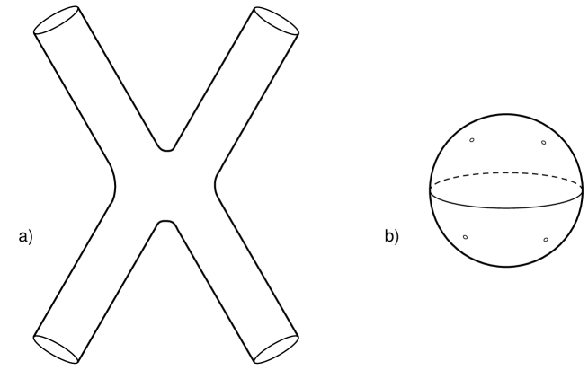
Figure 2: a) Tree closed string diagram describing four-point scattering. b) Its conformal equivalent, the four-punctured sphere

By a conformal transformation we can map the diagram to a sphere with four infinitesimal holes (punctures) (Fig. 2b). At each puncture we have to put appropriate boundary conditions that will specify which is the external physical state that participates in the interaction. In the language of the path integral we will have to insert a “vertex operator”, namely the appropriate wavefunction as we have done in the case of the point particle. Then, we will have to take the path-integral average of these vertex operators weighted with the Polyakov action on the sphere. In the operator language, this amplitude (S-matrix element) will be given by a correlation function of these vertex operators in the two-dimensional world-sheet quantum theory. We will also have to integrate over the positions of these vertex operators. On the sphere there are three conformal Killing vectors, which implies that there are three reparametrizations that have not been fixed. We can fix them by fixing the positions of three vertex operators. The positions of the rest are Teichmüller moduli and should be integrated over.

What is the vertex operator associated to a given physical state? This can be found directly from the two-dimensional world-sheet theory. The correct vertex operator will produce the appropriate physical state as it comes close to the out vacuum, but more on this will follow in the next section.

One more word about loop amplitudes. Consider the string diagram in Fig. 3a. This is the string generalization of a one-loop amplitude contribution to the scattering of four particles in Fig. 2a. Again by a conformal transformation it can be deformed into a torus with four punctures (Fig. 3b). The generalization is straightforward. An N-point amplitude (S matrix element) at g-loop order is given by the average of the N appropriate vertex operators, the average taken with the Polyakov action on a two-dimensional surface with g handles (genus g Riemann surface). For more details, we refer the reader to [5].

From this discussion, we have seen that the zero-, one- and two-point amplitudes on the sphere are not defined. This is consistent with the fact that such amplitudes do not exist on-shell. The zero-point amplitude at one loop is not defined either. When we will be talking about the one-loop vacuum amplitude below, we will implicitly consider the one-point dilaton amplitude at zero momentum.

6 Conformal field theory

We have seen so far that the world-sheet quantum theory that describes the bosonic string is a conformally invariant quantum field theory in two dimensions. In order to describe more general ground-states of the string, we will need to study this concept in more detail. In this chapter we will give a basic introduction to conformal field theory and its application in string theory. We will assume Euclidean signature in two dimensions. A more complete discussion can be found in [13].

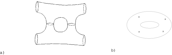
Figure 3: a) World-sheet relevant for the one-loop contribution to four-point scattering; b) Its conformal transform where the holes become punctures on a torus.

6.1 Conformal transformations

Under general coordinate transformations, $x\to x^{\prime}$, the metric transforms as

$$g_{\mu\nu}\to g^{\prime}_{\mu\nu}(x^{\prime})=\frac{\partial x^{\alpha}}{\partial x^{\prime\mu}}\frac{\partial x^{\beta}}{\partial x^{\prime\nu}}g_{\alpha\beta}(x)\,.$$

The group of conformal transformations, in any dimension, is then defined as the subgroup of these coordinate transformations that leave the metric invariant up to a scale change:

$$g_{\mu\nu}(x)\to g^{\prime}_{\mu\nu}(x^{\prime})=\Omega(x)g_{\mu\nu}(x)\,.$$ (6.1.1)

These are precisely the coordinate transformations that preserve the angle between two vectors, hence the name conformal transformations. Note that the Poincaré group is a subgroup of the conformal group (with $\Omega=1$).

We will examine the generators of these transformations. Under infinitesimal coordinate transformations, $x^{\mu}\to x^{\prime\mu}=x^{\mu}+\epsilon^{\mu}$, we obtain

$$ds^{\prime 2}=ds^{2}-(\partial_{\mu}\epsilon_{\nu}+\partial_{\nu}\epsilon_{\mu})dx^{\mu}dx^{\nu}\,.$$

For it to be a conformal transformation, the second term on the right-hand side has to be proportional to $\eta_{\mu\nu}$, or

$$\partial_{\mu}\epsilon_{\nu}+\partial_{\nu}\epsilon_{\mu}=\frac{2}{d}(\partial\cdot\epsilon)\eta_{\mu\nu}\,,$$ (6.1.2)

where the proportionality factor can be found by contracting both sides with $\eta^{\mu\nu}$. If we act on both sides of this equation with $\partial^{\mu}$ we obtain

$$\Box\epsilon_{\nu}+\left(1-\frac{2}{d}\right)\partial_{\nu}(\partial\cdot\epsilon)=0\,,$$

or if we act on both sides of (6.1.2) with $\Box=\partial_{\mu}\partial^{\mu}$ we obtain

$$\partial_{\mu}\Box\epsilon_{\nu}+\partial_{\nu}\Box\epsilon_{\mu}=\frac{2}{d}\eta_{\mu\nu}\Box(\partial\cdot\epsilon)\,.$$

With these two equations, we can write the constraints on the parameter as follows

$$\left[\eta_{\mu\nu}\Box+(d-2)\partial_{\mu}\partial_{\nu}\right]\partial\cdot\epsilon=0\,.$$ (6.1.3)

We can already see in (6.1.3) that $d=2$ will be a special case. Indeed for $d>2$, (6.1.3) implies that the parameter $\epsilon$ can be at most quadratic in $x$. We can then identify the following possibilities for $\epsilon$:

$$\epsilon^{\mu}=a^{\mu} \mbox{translations}\,,$$

$$\epsilon^{\mu}=\omega^{\mu}_{\nu}x^{\nu} \mbox{rotations}\quad(\omega_{\mu\nu}=-\omega_{\nu\mu})\,,$$ (6.1.4)

$$\epsilon^{\mu}=\lambda x^{\mu}$$ scale transformations

and

$$\epsilon^{\mu}=b^{\mu}x^{2}-2x^{\mu}(b\cdot x)\,,$$ (6.1.5)

which are the special conformal transformations. Thus, we have a total of

$$d+{\textstyle{1\over 2}}d(d-1)+1+d={\textstyle{1\over 2}}(d+2)(d+1)$$

parameters. In a space of signature $(p,q)$ with $d=p+q$, the Lorentz group is O(p,q).

Exercise: Show that the algebra of conformal transformations is isomorphic to the Lie algebra of O(p+1,q+1).

We will now investigate the special case $d=2$. The restriction that $\epsilon$ can be at most of second order does not apply anymore, but (6.1.2) in Euclidean space ($g_{\mu\nu}=\delta_{\mu\nu}$) reduces to

$$\partial_{1}\epsilon_{1}=\partial_{2}\epsilon_{2}\,,\quad\quad\partial_{1}\epsilon_{2}=-\partial_{2}\epsilon_{1}\,.$$ (6.1.6)

This can be further simplified by going to complex coordinates, $z,\bar{z}=x^{1}\pm ix^{2}$. If we define the complex parameters $\epsilon,\bar{\epsilon}=\epsilon_{1}\pm i\epsilon_{2}$, the equations for the parameters become

$$\partial\bar{\epsilon}=0\,,\quad\quad\bar{\partial}\epsilon=0\,,$$ (6.1.7)

where we used the short-hand notation $\bar{\partial}=\partial_{\bar{z}}$. This means that $\epsilon$ can be an arbitrary function of $z$, but it is independent of $\bar{z}$ and vice versa for $\bar{\epsilon}$. Globally, this means that conformal transformations in two dimensions consist of the analytic coordinate transformations

$$z\to f(z)\quad\mbox{and}\quad\bar{z}\to\bar{f}(\bar{z})\,.$$ (6.1.8)

We can expand the infinitesimal transformation parameter

$$\epsilon(z)=-\sum a_{n}z^{n+1}\,.$$

The generators corresponding to these transformations are then

$${\ell}_{n}=-z^{n+1}\partial_{z}\,,$$ (6.1.9)

i.e. ${\ell}_{n}$ generates the transformation with $\epsilon=-z^{n+1}$. The generators satisfy the following algebra

$$[{\ell}_{m},{\ell}_{n}]=(m-n){\ell}_{m+n}\,,\quad\quad[\bar{\ell}_{m},\bar{\ell}_{n}]=(m-n)\bar{\ell}_{m+n}\,,$$ (6.1.10)

and $[\bar{\ell}_{m},{\ell}_{n}]=0$. Thus, the conformal group in two dimensions is infinite-dimensional.

An interesting subalgebra of this algebra is spanned by the generators ${\ell}_{0,\pm 1}$ and $\bar{\ell}_{0,\pm 1}$. These are the only generators that are globally well-defined on the Riemann sphere $S^{2}=\hbox{\mybb C}\cup\infty$. They form the algebra of O(2,2)$\sim$SL(2,$\hbox{\mybb C})$. They generate the following transformations:

	Infinitesimal	Finite
Generator	transformation	transformation
${\ell}_{-1}$	$z\to z-\epsilon$	$z\to z+\alpha$	Translations
${\ell}_{0}$	$z\to z-\epsilon z$	$z\to\lambda z$	Scaling
${\ell}_{1}$	$z\to z-\epsilon z^{2}$	$z\to\frac{z}{1-\beta z}$	Special conformal

with equivalent expressions for the barred generators. From this, it is immediately clear that the generator $i(\ell_{0}-\bar{\ell}_{0})$ generates a rescaling of the phase or, in other words, it generates rotations in the $z$-plane. Dilatations are generated by $\ell_{0}+\bar{\ell}_{0}$. These transformations generated by ${\ell}_{0,\pm 1}$ can be summarized by the expression

$$z\to\frac{az+b}{cz+d}\,,$$ (6.1.11)

where $a,b,c,d\in\hbox{\mybb C}$ and $ad-bc=1$. This is the group SL(2,$\hbox{\mybb C})/\hbox{\mybb Z}_{2}$, where the $\hbox{\mybb Z}_{2}$ fixes the freedom to replace all parameters $a,b,c,d$ by minus themselves, leaving the transformation (6.1.11) unchanged. We will call this finite-dimensional subgroup of the conformal group the restricted conformal group.

6.2 Conformally invariant field theory

A two-dimensional theory will be called conformally invariant if the trace of its stress-tensor vanishes in the quantum theory in flat space. Such a theory has the following properties:

1) There is an (infinite) set of fields $\{A_{i}\}$. In particular, this set will contain all the derivatives of the fields.

2) There exists a subset $\{\phi_{j}\}\subset\{A_{i}\}$, called quasi-primary fields, that transforms under $restricted$ conformal transformations

$$z\to f(z)={az+b\over cz+d}\;\;\;,\;\;\;\bar{z}\to\bar{f}(\bar{z})={\bar{a}\bar{z}+\bar{b}\over\bar{c}\bar{z}+\bar{d}}$$ (6.2.1)

in the following way,

$$\Phi(z,\bar{z})\to\left(\frac{\partial f}{\partial z}\right)^{h}\left(\frac{\partial\bar{f}}{\partial\bar{z}}\right)^{\bar{h}}\Phi\left(f(z),\bar{f}(\bar{z})\right)\,.$$ (6.2.2)

As we shall see later all fields that are not derivatives of other fields are quasi-primary.

3) Finally there are the so-called primary fields, which transform as in (6.2.2) for all conformal transformations; $h,\bar{h}$ are real-valued ($\bar{h}$ is not the complex conjugate of $h$). Note that this transformation property is very similar to the transformation property of tensors. As for tensors, the expression

$$\Phi(z,\bar{z})dz^{h}d\bar{z}^{\bar{h}}$$

is invariant under conformal transformations; $(h,\bar{h})$ are the conformal weights of the primary field.

The theory is covariant under conformal transformations. Consequently, the correlation functions satisfy

$$\left\langle\,\prod_{i=1}^{N}\Phi_{i}(z_{i},\bar{z}_{i})\,\right\rangle=\prod_{i=1}^{N}\left(\frac{\partial f}{\partial z}\right)^{h_{i}}_{z\to z_{i}}\left(\frac{\partial\bar{f}}{\partial\bar{z}}\right)^{\bar{h}_{i}}_{\bar{z}\to\bar{z}_{i}}\left\langle\,\prod_{j=1}^{N}\Phi_{j}\left(f(z_{j}),\bar{f}(\bar{z}_{j})\right)\right\rangle\;.$$ (6.2.3)

As we shall see later on, the conformal anomaly spontaneously breaks the invariance of the full conformal group. On the sphere, the unbroken subgroup is the restricted conformal group and (6.2.3) is, thus, valid only for SL(2,$\hbox{\mybb C})$. However, there will be Ward identities that will encode the full conformal covariance of the theory.

Infinitesimally, under $z\to z+\epsilon(z)$ and $\bar{z}\to\bar{z}+\bar{\epsilon}(\bar{z})$, a primary field transforms as

$$\delta_{\epsilon,\bar{\epsilon}}\Phi(z,\bar{z})=\left[(h\partial\epsilon+\epsilon\partial)+(\bar{h}\bar{\partial}\bar{\epsilon}+\bar{\epsilon}\bar{\partial})\right]\Phi(z,\bar{z})\,,$$ (6.2.4)

and the two-point function $G^{(2)}(z_{i},\bar{z}_{i})=\langle\,\Phi(z_{1},\bar{z}_{1})\Phi(z_{2},\bar{z}_{2})\,\rangle$ transforms as

$$\delta_{\epsilon,\bar{\epsilon}}G^{(2)}(z_{i},\bar{z}_{i})=\langle\,\delta_{\epsilon,\bar{\epsilon}}\Phi_{1},\Phi_{2}\,\rangle+\langle\,\Phi_{1},\delta_{\epsilon,\bar{\epsilon}}\Phi_{2}\,\rangle=0\,.$$

If we put these two together, it results in the following differential equation for the two-point function

$$\left[\left(\epsilon(z_{1})\partial_{z_{1}}+h_{1}\partial\epsilon(z_{1})+\epsilon(z_{2})\partial_{z_{2}}+h_{2}\partial\epsilon(z_{2})\right)+\left(\mbox{barred terms}\right)\right]G^{(2)}(z_{i},\bar{z}_{i})=0\,.$$ (6.2.5)

We can now use the series expansion of $\epsilon(z)$ to analyze this equation. If we first take $\epsilon(z)=1$ and $\bar{\epsilon}(\bar{z})=1$ (remember, this corresponded to translations), then (6.2.5) tells us that $G^{(2)}(z_{i},\bar{z}_{i})$ only depends on $z_{12}=z_{1}-z_{2}$, $\bar{z}_{12}=\bar{z}_{1}-\bar{z}_{2}$. This is not very surprising because in a translationally invariant theory we would expect the correlation functions to only depend on the relative distance. If we next use $\epsilon(z)=z$, $\bar{\epsilon}(\bar{z})=\bar{z}$ (rotational invariance), we find $G^{(2)}\sim 1/(z_{12}^{h_{1}+h_{2}}\bar{z}_{12}^{\bar{h}_{1}+\bar{h}_{2}})$ and if we finally use $\epsilon(z)=z^{2}$ (special conformal transformation) we find the restriction $h_{1}=h_{2}=h$ and $\bar{h}_{1}=\bar{h}_{2}=\bar{h}$. The conclusion is that the two-point function is completely fixed up to a constant:

$$G^{(2)}(z_{i},\bar{z}_{i})=\frac{C_{12}}{z_{12}^{2h}\bar{z}_{12}^{2\bar{h}}}\,.$$ (6.2.6)

This constant can be set to 1, by normalizing the operators.

A similar analysis can be done for the three-point function and it turns out to be also completely determined up to a constant:

Exercise: Solve the Ward identities and show that the most general form allowed for the three-point function is

$$G^{(3)}(z_{i},\bar{z}_{i})=\frac{C_{123}}{z_{12}^{\Delta_{12}}z_{23}^{\Delta_{23}}z_{31}^{\Delta_{31}}\bar{z}_{12}^{\bar{\Delta}_{12}}\bar{z}_{12}^{\bar{\Delta}_{12}}\bar{z}_{12}^{\bar{\Delta}_{12}}}\,,$$ (6.2.7)

where $\Delta_{12}=h_{1}+h_{2}-h_{3}$, $\bar{\Delta}_{12}=\bar{h}_{1}+\bar{h}_{2}-\bar{h}_{3}$, etc.

The next correlation function, however, the four-point function, is not fully determined. Conformal invariance restricts it, using the procedure outlined above, to have the following form

$$G^{(4)}(z_{i},\bar{z}_{i})=f(x,\bar{x})\prod_{i<j}z_{ij}^{-(h_{i}+h_{j})+h/3}\prod_{i<j}\bar{z}_{ij}^{-(\bar{h}_{i}+\bar{h}_{j})+\bar{h}/3}\,,$$ (6.2.8)

where $h=\sum h_{i}$, $\bar{h}=\sum\bar{h}_{i}$. The function $f$ is arbitrary, but only depends on the cross-ratio $x=z_{12}z_{23}/z_{13}z_{24}$ and $\bar{x}$.

The general N-point function of quasiprimary fields on the sphere

$$G^{N}(z_{1},\bar{z}_{1},\dots z_{N},\bar{z}_{N})=\left\langle\prod_{i=1}^{N}\Phi_{i}(z_{i},\bar{z}_{i})\right\rangle$$ (6.2.9)

satisfies the following constraints coming from SL(2,$\hbox{\mybb C})$ covariance

$$\sum_{i=1}^{N}\partial_{i}~{}G^{N}=0\,,$$ (6.2.10)

$$\sum_{i=1}^{N}(z_{i}\partial_{i}+h_{i})~{}G^{N}=0\,,$$ (6.2.11)

$$\sum_{i=1}^{N}(z_{i}^{2}\partial_{i}+2z_{i}h_{i})~{}G^{N}=0$$ (6.2.12)

and similar ones with $z_{i}\to\bar{z}_{i}$, $h_{i}\to\bar{h}_{i}$. These are the Ward identities reflecting SL(2,$\hbox{\mybb C})$ invariance of the correlation functions on the sphere.

6.3 Radial quantization

We will now study the Hilbert space of a conformally invariant theory. We start from a two-dimensional Euclidean space with coordinates $\tau$ and $\sigma$. (Note that we can go from a two-dimensional Euclidean space to Minkowski space by means of a Wick rotation, $\tau\to i\tau$.) To avoid IR problems we will compactify the space direction, $\sigma=\sigma+2\pi$, and the two-dimensional space becomes a cylinder. Next, we make the conformal transformation

$$z=e^{\tau+i\sigma}\,,\quad\quad\bar{z}=e^{\tau-i\sigma}\,,$$

which maps the cylinder onto the complex plane (topologically a sphere) as shown in Fig. 4.

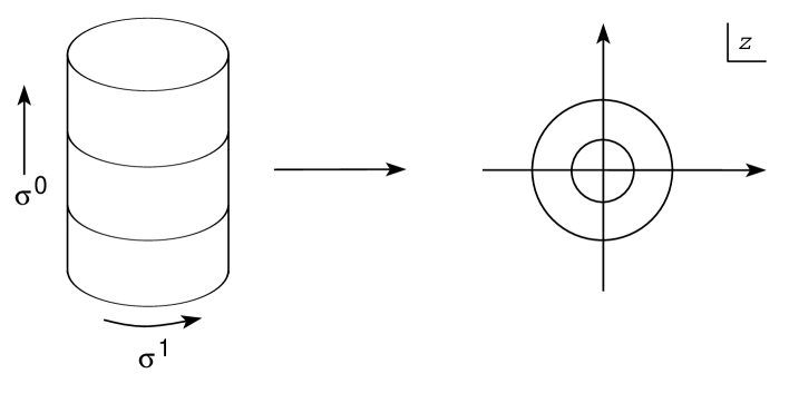
Figure 4: The map from the cylinder to the compactified complex plane

Surfaces of equal time on the cylinder will become circles of equal radius on the complex plane. This means that the infinite past ($\tau=-\infty$) gets mapped onto the origin of the plane ($z=0$) and the infinite future becomes $z=\infty$. Time reversal becomes $z\to 1/z^{*}$ on the complex plane, and parity $z\to z^{*}$.

We already saw that $\ell_{0}$ was the generator of dilatations on the cylinder, $z\to\lambda z$ so $\ell_{o}+\bar{\ell}_{0}$ will move us in the radial direction on the plane, which corresponds to the time direction on the cylinder. This means that the dilatation operator is the Hamiltonian of our system

$$H=\ell_{0}+\bar{\ell}_{0}\,.$$

An integral over the space direction $\sigma$ will become a contour integral on the complex plane. This enables us to use all the powerful techniques developed in complex analysis.

Infinitesimal coordinate transformations are generated by the stress-tensor, which is traceless in the case of a Conformal Field Theory (CFT),

$$T_{\mu}{}^{\mu}=0.$$ (6.3.1)

In complex coordinates this means that the stress-tensor has non-vanishing components $T_{zz}$ and $T_{\bar{z}\bar{z}}$, while $T_{z\bar{z}}=0$ since $T_{z\bar{z}}$ is the trace of the stress-tensor. This can be shown by expressing them back in Euclidean coordinates, $z=x+iy$,

$$T_{z\bar{z}}=T_{\bar{z}z}={\textstyle{1\over 4}}(T_{00}+T_{11})={\textstyle{1\over 4}}T_{\mu}{}^{\mu}\,.$$

The conservation law $\partial^{\mu}T_{\mu\nu}=0$ gives us, together with the traceless condition,

$$\partial_{z}T_{\bar{z}\bar{z}}=0\quad\mbox{and}\quad\partial_{\bar{z}}T_{zz}=0\,,$$ (6.3.2)

which implies that the two non-vanishing components of the stress-tensor are holomorphic and antiholomorphic respectively:

$$T(z)\equiv T_{zz}\quad\mbox{and}\quad\bar{T}(\bar{z})\equiv T_{\bar{z}\bar{z}}\,.$$ (6.3.3)

Thus, we can construct an infinite number of conserved currents, because if $T(z)$ is conserved, then $\epsilon(z)T(z)$ is also conserved, for every holomorphic function $\epsilon(z)$.

These currents produce the following conserved charges

$$Q_{\epsilon}=\frac{1}{2\pi i}\oint dz\epsilon(z)T(z)\;\;\;,\;\;\;Q_{\bar{\epsilon}}=\frac{1}{2\pi i}\oint d\bar{z}\bar{\epsilon}(\bar{z})\bar{T}(\bar{z})\,.$$ (6.3.4)

These charges are the generators of the infinitesimal conformal transformations

$$z\to z+\epsilon(z)\,,\quad\quad\quad\bar{z}\to\bar{z}+\bar{\epsilon}(\bar{z})\,.$$

The variation of fields under these transformations is given, as usual, by the commutator of the fields with the generators:

$$\delta_{\epsilon,\bar{\epsilon}}\Phi(z,\bar{z})=\left[Q_{\epsilon}+Q_{\bar{\epsilon}},\Phi(z,\bar{z})\right]\,.$$ (6.3.5)

We know that products of operators are only well-defined in a quantum theory if they are time-ordered. The analog of this in radial quantization on the complex plane is radial ordering. The radial-ordering operator $R$ is defined as:

$$R(A(z)B(w))=\left\{\begin{array}[]{cc}A(z)B(w)&|z|>|w|\\ (-1)^{F}B(w)A(z)&|z|<|w|\end{array}\;.\right.$$ (6.3.6)

In the case of fermionic operators, there appears of course a minus sign if we interchange them. With the help of this ordering we can write an equal-time commutator of an operator with a spatial integral over another operator as a contour integral over the radially-ordered product of the two operators:

$$\left[\int d\sigma B,A\right]=\oint dzR(B(z)A(w))$$

as shown in Fig. 5. This means that we can rewrite (6.3.5) as

$$\delta_{\epsilon,\bar{\epsilon}}\Phi(z,\bar{z}) = \frac{1}{2\pi i}\oint\left(dz\epsilon(z)R(T(z)\Phi(w,\bar{w}))+d\bar{z}\bar{\epsilon}(\bar{z})R(\bar{T}(\bar{z})\Phi(w,\bar{w}))\right)$$

$$= \left[(h\partial\epsilon(w)+\epsilon(w)\partial)+(\bar{h}\bar{\partial}\bar{\epsilon}(\bar{w})+\bar{\epsilon}(\bar{w})\bar{\partial})\right]\Phi(w,\bar{w})\,,$$

where the last line is the desired result copied from (6.2.4). This equality will only hold if $T$ and $\bar{T}$ have the following short-distance singularities with $\Phi$:

$$R(T(z)\Phi(w,\bar{w}))=\frac{h}{(z-w)^{2}}\Phi(w,\bar{w})+\frac{1}{z-w}\partial_{w}\Phi(w,\bar{w})+\dots\,,$$ (6.3.7)

$$R(\bar{T}(\bar{z})\Phi(w,\bar{w}))=\frac{\bar{h}}{(\bar{z}-\bar{w})^{2}}\Phi(w,\bar{w})+\frac{1}{\bar{z}-\bar{w}}\partial_{\bar{w}}\Phi(w,\bar{w})+\dots\,,$$ (6.3.8)

where the dots (which we write at first, but end up being implicit) denote regular terms. From now on we shall drop the $R$ symbol and assume that the operator product expansion (OPE) is always radially ordered. The OPE with the stress-tensor can be used as a definition of a conformal field of weight $(h,\bar{h})$ instead of (6.2.2).

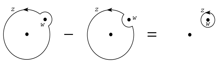
Figure 5: Rearrangement of contours relevant for commutators.

We will describe here the general Ward identities for insertions of the stress-tensor. Consider the correlation function

$$F^{N}(z,z_{i},\bar{z}_{i})=\left\langle T(z)\prod_{i=1}^{N}\Phi_{i}(z_{i},\bar{z}_{i})\right\rangle\,,$$ (6.3.9)

where $\Phi_{i}$ are primary fields. Viewed as a function of $z$, $F^{N}$ is meromorphic with poles when $z\to z_{i}$. The residues of these poles can be calculated with the help of (6.3.8). A meromorphic function on the sphere is uniquely specified by its poles and residues. Thus, we obtain

$$F^{N}(z,z_{i},\bar{z}_{i})=\sum_{i=1}^{N}\left({h_{i}\over(z-z_{i})^{2}}+{\partial_{z_{i}}\over z-z_{i}}\right)\left\langle\prod_{i=1}^{N}\Phi_{i}(z_{i},\bar{z}_{i})\right\rangle\,.$$ (6.3.10)

This Ward identity expresses correlation functions of primary fields with an insertion of the stress-tensor in terms of the correlator of the primary fields themselves. Multiple insertions can also be handled using in addition (6.5.1).

In general, the product of two operators can be expanded in terms of a complete set of orthonormal local operators

$$\Phi_{i}(z,\bar{z})\Phi_{j}(w,\bar{w})=\sum_{k}C_{ijk}(z-w)^{h_{k}-h_{i}-h_{j}}(\bar{z}-\bar{w})^{\bar{h}_{k}-\bar{h}_{i}-\bar{h}_{j}}\Phi_{k}(w,\bar{w})\,,$$ (6.3.11)

where the numerical constants $C_{ijk}$ can be shown to coincide with the constants in the three-point function $\langle\,\Phi_{i}\Phi_{j}\Phi_{k}\,\rangle$. This is true in any quantum field theory; here, however, because of conformal invariance there is no mass scale that appears in the OPE. This type of expansion can be thought of as a way to encode the correlation functions, since knowledge of (6.3.11) determines them completely in a unitary theory and vice versa.

6.4 Example: the free boson

The action for a non-compact free boson in two dimensions as we encountered it in string theory is

$$S=\frac{1}{4\pi}\int d^{2}z~{}\partial X\bar{\partial}X\,.$$ (6.4.1)

The field $X(z,\bar{z})$ has the propagator

$$\langle\,X(z,\bar{z})X(w,\bar{w})\,\rangle=-\log(|z-w|^{2}\mu^{2})\,.$$ (6.4.2)

This is obtained by taking the massless limit of the massive scalar propagator in two dimensions; $\mu$ is an IR cutoff. Equation (6.4.2) can be obtained by starting with the massive propagator, with mass $\mu$, and taking the limit $\mu\to 0$, keeping terms that do not vanish in the limit. The dependence on $\mu$ should disappear from correlation functions. Note that $X$ itself is not a conformal field since its correlation functions are IR-divergent. Its derivative $\partial_{z}X$, however, is well behaved. The OPE of the derivative with itself is

$$\partial_{z}X(z)\partial_{w}X(w) = \partial_{z}\partial_{w}\langle XX\rangle+:\partial_{z}X\partial_{w}X:$$ (6.4.3)

$$= -\frac{1}{(z-w)^{2}}+:\partial_{z}X\partial_{w}X:$$

and $\partial_{z}X$ is a conformal field of weight $(1,0)$. Note that $\mu$ has disappeared. We will now calculate its OPE with the stress-tensor.

According to the action (6.4.1) the stress-tensor for the free boson is given by

$$T(z)=-{\textstyle{1\over 2}}:\partial X\partial X:=-{\textstyle{1\over 2}}\lim_{z\to w}\left[\partial_{z}X\partial_{w}X+\frac{1}{(z-w)^{2}}\right]\,,$$ (6.4.4)

$$\bar{T}(\bar{z})=-{\textstyle{1\over 2}}:\bar{\partial}X\bar{\partial}X:=-{\textstyle{1\over 2}}\lim_{\bar{z}\to\bar{w}}\left[\partial_{\bar{z}}X\partial_{\bar{w}}X+\frac{1}{(\bar{z}-\bar{w})^{2}}\right]\,.$$ (6.4.5)

Using Wick’s theorem, we can calculate

$$T(z)\partial X(w) = -{\textstyle{1\over 2}}:\partial X(z)\partial X(z):\partial X(w)$$ (6.4.6)

$$= -\partial X(z)\langle\partial X(z)\partial X(w)\rangle+\dots$$

$$= \partial X(z)\frac{1}{(z-w)^{2}}+\dots$$

$$= \frac{\partial X(w)}{(z-w)^{2}}+\frac{1}{z-w}\partial^{2}X(w)+\dots\,,$$

where the dots indicate terms that are not singular as $z\to w$. Similarly we find $\bar{T}\partial X=\mbox{regular}$. Thus, $\partial X$ is a $(1,0)$ primary field. In the same way we find that $\bar{\partial}X$ is a $(0,1)$ primary field.

Are there any other primary fields? The answer is yes. There are certainly several, constructed out of products of derivatives of $X$. We will consider another interesting class, the “vertex” operators $V_{a}(z)$=$:e^{iaX(z)}:$. The OPE with the stress-tensor is

$$T(z)V_{a}(w,\bar{w})=-{\textstyle{1\over 2}}:\partial X(z)\partial X(z):\sum_{n=0}^{\infty}\frac{i^{n}a^{n}}{n!}:X^{n}(w,\bar{w}):\,.$$ (6.4.7)

For all terms in the expansion there can be either one or two contractions. We obtain

$$T(z)V_{a}(w) = -{\textstyle{1\over 2}}\left[ia\partial\langle XX\rangle\right]^{2}e^{iaX(w)}-{\textstyle{1\over 2}}2ia:\partial X(z)\partial\langle XX\rangle e^{iaX(w)}:+\dots$$ (6.4.8)

$$= \frac{a^{2}/2}{(z-w)^{2}}e^{iaX(w)}+\frac{ia\partial X(z)}{z-w}e^{iaX(w)}+\dots$$

$$= \frac{a^{2}/2}{(z-w)^{2}}V_{a}(w)+\frac{1}{z-w}\partial V_{a}(w)+\dots\,.$$

Thus, the vertex operator $V_{a}$ is a conformal field of weight $(a^{2}/2,0)$.

Consider now a correlation function of vertex operators

$$G^{N}=\left\langle\prod_{i=1}^{N}V_{a_{i}}(z_{i},\bar{z}_{i})\right\rangle=\exp\left[{1\over 2}\sum_{i,j=1;i\neq j}^{N}a_{i}a_{j}\langle X(z_{i},\bar{z}_{i})X(z_{j},\bar{z}_{j})\rangle\right]\,,$$ (6.4.9)

where the second step in the above formula is due to the fact that we have a free (Gaussian) field theory. Using the propagator (6.4.2) we can see that the IR divergences cancel only if

$$\sum_{i}a_{i}=0.$$ (6.4.10)

This a charge-conservation condition.

For the two-point function we obtain

$$\langle V_{a}(z)V_{-a}(w)\rangle = \langle:e^{iaX(z)}:\,:e^{-iaX(w)}:\rangle$$ (6.4.11)

$$= e^{-a^{2}\log|z-w|^{2}}=\frac{1}{|z-w|^{2a^{2}}}\,,$$

which confirms that $a^{2}=2h=2\bar{h}$.

In this theory the operator $i\partial X$ is a U(1) current, which is chirally conserved. It is associated to the symmetry of the action under $X\to X+\epsilon$. The zero mode of the current is the charge operator. From

$$i\partial_{z}X~{}V_{a}(w,\bar{w})=a~{}{V_{a}(w,\bar{w})\over(z-w)}+{\rm finite}$$ (6.4.12)

we can tell that the operator $V_{a}$ carries charge $a$. The charge-conservation condition (6.4.10) is precisely due to the U(1) invariance of the theory. In the case of string theory, this type of U(1) invariance is essentially momentum conservation.

6.5 The central charge

The stress-tensor $T_{\mu\nu}$ is conserved so it has scaling dimension two. In particular $T(z)$ has conformal weight (2,0) and $\bar{T}(\bar{z})$ (0,2). They are obviously quasiprimary fields. From these properties we can write the most general OPE between two stress-tensors compatible with conservation (holomorphicity) and conformal invariance.

$$T(z)T(w)=\frac{c/2}{(z-w)^{4}}+2\frac{T(w)}{(z-w)^{2}}+\frac{\partial T(w)}{z-w}+\dots\,.$$ (6.5.1)

The fourth-order pole can only be a constant. This constant has to be positive in a unitary theory since $\langle T(z)T(w)\rangle=c/2(z-w)^{4}$. There can be no third-order pole since the OPE has to be symmetric under $z\leftrightarrow w$. Finally the rest of the singular terms are fixed by the fact that $T$ has conformal weight (2,0). We have a similar OPE for $\bar{T}$ with $z\to\bar{z}$ and $c\to\bar{c}$ and

$$T(z)\bar{T}(\bar{w})={\rm regular}\,.$$ (6.5.2)

Comparing (6.5.1) with (6.3.8) we can conclude that $T(z)$ itself is not a primary field due to the presence of the most singular term. The constant $c$ is called the (left) central charge and $\bar{c}$ the right central charge. Modular invariance implies that for a left-right asymmetric theory $c-\bar{c}=0(\,\,{\rm mod}\,\,24)$ and two-dimensional Lorentz invariance requires $c=\bar{c}$.

We will calculate the value of $c,\bar{c}$ for the free boson theory. With the stress-tensor $T(z)=-{\textstyle{1\over 2}}:\partial X\partial X:$ we can calculate the OPE

$$T(z)T(w) = {\textstyle{1\over 4}}\left\{2\left(\partial\partial\langle XX\rangle\right)^{2}+4:\partial X(z)\partial X(w):\partial\partial\langle XX\rangle+\dots\right\}\quad\quad$$ (6.5.3)

$$= \frac{1/2}{(z-w)^{4}}+\frac{2}{(z-w)^{2}}T(w)+\frac{1}{z-w}\partial T(w)+\dots\,,$$

and we see that a single free boson has central charge $c=\bar{c}=1$. In the bosonic string theory we have $d$ free bosons, consequently the central charge is $c=\bar{c}=d$.

Exercise: Consider another (2,0) operator

$$\tilde{T}=-{\textstyle{1\over 2}}:\partial X\partial X:+iQ\partial^{2}X\,,$$

where the second term is a total derivative. This is the stress-tensor of a modified theory for the free boson where there is some background charge $Q$. Follow the same procedure as above and show that the OPE of the two stress-tensors is again of the same form as (6.5.1), but with central charge:

$$c=1-12Q^{2}\,.$$ (6.5.4)

Verify that the conformal weight of the vertex operator $V_{\alpha}$ is now $\Delta=\alpha(\alpha-2Q)/2$. In particular, $V_{\alpha}$ and $V_{-\alpha+2Q}$ have the same conformal weight. The charge neutrality condition (6.4.10) now becomes $\sum_{i}\alpha_{i}=2Q$.

6.6 The free fermion

We will now analyze the conformal field theory, which describes a free massless fermion. In two dimensions, it is possible to have spinors that are both Majorana and Weyl, and these will have only one component. The gamma matrices can be represented by the Pauli matrices, i.e. $\gamma^{1}=\sigma^{1}$, $\gamma^{2}=\sigma^{2}$, so that the chirality projectors are ${\textstyle{1\over 2}}(1\pm\sigma^{3})$. The Dirac operator becomes

$${\partial/}=\sigma^{1}\partial_{1}+\sigma^{2}\partial_{2}=\left(\begin{array}[]{cc}0&\partial_{1}-i\partial_{2}\\ \partial_{1}+i\partial_{2}&0\end{array}\right)\sim\left(\begin{array}[]{cc}0&\partial\\ \bar{\partial}&0\end{array}\right).$$ (6.6.1)

The action for a Majorana spinor $\left(\begin{array}[]{c}\psi\\ \bar{\psi}\end{array}\right)$ is

$$S=-\frac{1}{8\pi}\int d^{2}z(\psi\bar{\partial}\psi+\bar{\psi}\partial\bar{\psi}).$$ (6.6.2)

The equations of motion are

$$\bar{\partial}\psi=\partial\bar{\psi}=0,$$ (6.6.3)

which means that the left and right chiralities are represented by a holomorphic and an anti-holomorphic spinor, respectively.

The operator product expansion of $\psi$ and $\bar{\psi}$ with themselves can be found either by transforming the action into momentum space or by explicitly writing down the most general power expression with the correct conformal dimension. They are given by

$$\psi(z)\psi(w)=\frac{1}{z-w}\;\;\;,\;\;\;\bar{\psi}(\bar{z})\bar{\psi}(\bar{w})=\frac{1}{\bar{z}-\bar{w}}\,.$$ (6.6.4)

Up to a constant factor, the only expressions with conformal dimension $(2,0)$ and $(0,2)$ respectively are

$$T(z)=-{\textstyle{1\over 2}}:\psi(z)\partial\psi(z):\;\;\;,\;\;\;\bar{T}(\bar{z})=-{\textstyle{1\over 2}}:\bar{\psi}(\bar{z})\bar{\partial}\bar{\psi}(\bar{z}):\,.$$ (6.6.5)

This stress-tensor has the correct operator product expansion

$$T(z)T(w)=\frac{1/4}{(z-w)^{4}}+\frac{2}{(z-w)^{2}}T(w)+\frac{1}{z-w}\partial T(w),$$ (6.6.6)

and a similar expression for $\bar{T}(\bar{z})$, so that $c=\bar{c}={\textstyle{1\over 2}}$.

Exercise: By calculating the expansions of $T(z)\psi(w)$ and $\bar{T}(\bar{z})\bar{\psi}(\bar{w})$, show that $\psi$ and $\bar{\psi}$ are primary fields of conformal weight $({\textstyle{1\over 2}},0)$ and $(0,{\textstyle{1\over 2}})$, respectively.

6.7 Mode expansions

We will write the mode expansion for the stress-tensor as

$$T(z)=\sum_{n\in\hbox{\mybb Z}}z^{-n-2}L_{n}\;\;\;,\;\;\;\bar{T}(\bar{z})=\sum_{n\in\hbox{\mybb Z}}\bar{z}^{-n-2}\bar{L}_{n}.$$ (6.7.1)

The exponent $-n-2$ is chosen such that for the scale change $z\rightarrow\frac{z}{\lambda}$, under which $T(z)\rightarrow\lambda^{2}T\left(\frac{z}{\lambda}\right)$, we have $L_{-n}\rightarrow\lambda^{n}L_{-n}$. $L_{-n}$ and $\bar{L}_{-n}$, then have scaling dimension $n$. If we consider a theory on a closed string world-sheet, the transformation from the Euclidean space cylinder to the complex plane is given by

$$w=\tau+i\sigma\rightarrow z=e^{w}.$$ (6.7.2)

For a holomorphic field $\Phi$ with conformal weight $h$, we would write

$$\Phi_{\mbox{\tiny cyl}}(w)=\sum_{n\in\hbox{\mybb Z}}\phi_{n}e^{-nw}=\sum_{n\in\hbox{\mybb Z}}\phi_{n}e^{in(i\tau-\sigma)}=\sum_{n\in\hbox{\mybb Z}}\phi_{n}z^{-n}.$$ (6.7.3)

When going to the plane and using (6.2.2) this becomes, for primary fields:

$$\Phi(z)=\sum_{n\in\hbox{\mybb Z}}\phi_{n}z^{-n-h}.$$ (6.7.4)

Non-primary fields also have an inhomogeneous piece in (6.2.2). In particular the correct transformation of the stress-tensor is [14]

$$T(z)\to(f^{\prime})^{2}T(f(z))+{c\over 12}\left[{f^{\prime\prime\prime}\over f^{\prime}}-{3\over 2}\left({f^{\prime\prime}\over f^{\prime}}\right)^{2}\right]\,.$$ (6.7.5)

This justifies the expansion of the stress-tensor (6.7.1).

The mode expansion can be inverted by

$$L_{n}=\oint\frac{dz}{2\pi i}z^{n+1}T(z)\;\;\;,\;\;\;\bar{L}_{n}=\oint\frac{d\bar{z}}{2\pi i}\bar{z}^{n+1}\bar{T}(\bar{z}).$$ (6.7.6)

The operator product expansions of $T(z)T(w)$ and $\bar{T}(\bar{z})\bar{T}(\bar{w})$ can now be written in terms of the modes. We have

$$[L_{n},L_{m}] = \left(\oint\frac{dz}{2\pi i}\oint\frac{dw}{2\pi i}-\oint\frac{dw}{2\pi i}\oint\frac{dz}{2\pi i}\right)z^{n+1}T(z)w^{m+1}T(w)$$ (6.7.7)

$$= \oint\frac{dw}{2\pi i}\oint_{C_{w}}\frac{dz}{2\pi i}z^{n+1}w^{m+1}\left(\frac{c/2}{(z-w)^{4}}+\frac{2T(w)}{(z-w)^{2}}+\frac{\partial T(w)}{z-w}+\ldots\right)$$

$$= \oint\frac{dw}{2\pi i}\left(\frac{c}{12}(n+1)n(n-1)w^{n-2}w^{m+1}+\right.$$

$$\left.\quad\quad+2~{}(n+1)w^{n}w^{m+1}T(w)+w^{n+1}w^{m+1}\partial T(w)\right)\,.$$

The residue of the first term comes from $\left.\frac{1}{3!}\partial^{3}_{z}z^{n+1}\right|_{z=w}=\frac{1}{6}(n+1)n(n-1)w^{n-2}$. We integrate the last term by parts and combine it with the second term. This gives $(n-m)w^{n+m+1}T(w)$. Performing the $w$ integration leads to the Virasoro algebra

$$[L_{n},L_{m}]=(n-m)L_{n+m}+\frac{c}{12}(n^{3}-n)\delta_{n+m,0}.$$ (6.7.8)

The analogous calculation for $\bar{T}(\bar{z})$ yields

$$[\bar{L}_{n},\bar{L}_{m}]=(n-m)\bar{L}_{n+m}+\frac{\bar{c}}{12}(n^{3}-n)\delta_{n+m,0}.$$ (6.7.9)

Since $T\bar{T}$ has no singularities in its OPE,

$$[L_{n},\bar{L}_{m}]=0.$$ (6.7.10)

Every conformally invariant theory realizes the conformal algebra, and its spectrum forms representations of it. For $c=\bar{c}=0$, it reduces to the classical algebra. A consequence of the conformal anomaly is that

$$T^{\alpha}_{\alpha}={c\over 96\pi^{3}}\sqrt{g}~{}R^{(2)},$$ (6.7.11)

where $R^{(2)}$ is the two-dimensional scalar curvature. In a generic non-conformally invariant theory the trace can be a generic function of its various fields. In a CFT it is proportional only to the scalar curvature. This implies that in a CFT with $c\not=0$ the theory depends on the conformal factor of the metric, but in a very specific form implied by (6.7.11). If we remember that the stress-tensor is the variation of the action with respect to the metric, we can integrate (6.7.11) to obtain the dependence of the quantum theory on the conformal factor. Let $\hat{g}_{\alpha\beta}=e^{\phi}g_{\alpha\beta}$. Then

$$\int[DX]_{\hat{g}}e^{-S[\hat{g}_{\alpha\beta},X]}=e^{-cS_{L}[g_{\alpha\beta},\phi]}\int[DX]_{g}e^{-S[g_{\alpha\beta},X]}\,,$$ (6.7.12)

where $X$ is a generic set of fields and

$$S_{L}[g_{\alpha\beta},\phi]={1\over 96\pi}\int\sqrt{\det g}g^{\alpha\beta}\partial_{\alpha}\phi\partial_{\beta}\phi+{1\over 48\pi}\int\sqrt{\det g}R^{(2)}~{}\phi\,.$$ (6.7.13)

This is the Liouville action. In critical string theory, the ghost system cancels the central charge of the string coordinates and the full theory is independent of the scale factor.

6.8 The Hilbert space

To describe the Hilbert space we will use the standard formalism of in and out states of quantum field theory adapted to our coordinate system. For quasi-primary fields $A(z,\bar{z})$, the in-states are defined as

$$|A_{\mbox{\tiny in}}\rangle=\lim_{\tau\rightarrow-\infty}A(\tau,\sigma)|0\rangle=\lim_{z\rightarrow 0}A(z,\bar{z})|0\rangle.$$ (6.8.1)

For the out-states, we need a description in the neighborhood of $z\rightarrow\infty$. If we define $z=\frac{1}{w}$, then this is the point $w=0$. The map $f:w\rightarrow z=\frac{1}{w}$ is a conformal transformation, under which $A(z,\bar{z})$ transforms as

$$\tilde{A}(w,\bar{w})=A(f(w),\bar{f}(\bar{w}))(\partial f(w))^{h}(\bar{\partial}\bar{f}(\bar{w}))^{\bar{h}}.$$ (6.8.2)

Substituting $f(w)=\frac{1}{w}$, we find

$$\tilde{A}(w,\tilde{w})=A\left(\frac{1}{w},\frac{1}{\bar{w}}\right)(-w^{-2})^{h}(-\bar{w}^{-2})^{\bar{h}}.$$ (6.8.3)

It is natural to define

$$\langle A_{\mbox{\tiny out}}|=\lim_{w,\bar{w}\rightarrow 0}\langle 0|\tilde{A}(w,\bar{w}).$$ (6.8.4)

We would like $\langle A_{\mbox{\tiny out}}|$ to be the Hermitian conjugate of $|A_{\mbox{\tiny in}}\rangle$. Hermitian conjugation of operators of weight $(h,\bar{h})$ is defined by

$$\left[A(z,\bar{z})\right]^{\dagger}=A\left(\frac{1}{\bar{z}},\frac{1}{z}\right)\bar{z}^{-2h}z^{-2\bar{h}}.$$ (6.8.5)

This definition finds its justification in the continuation from Euclidean space back to Minkowski space. The missing factor of $i$ in Euclidean time evolution $A(\sigma,\tau)=e^{\tau H}A(\sigma,0)e^{-\tau H}$ must be compensated for in the definition of the adjoint by a Euclidean time reversal, which is implemented on the plane by $z\rightarrow 1/z^{\ast}$. With the definition (6.8.5), we find

$$\langle A_{\mbox{\tiny out}}| = \lim_{w\rightarrow 0}\langle 0|\tilde{A}(w,\bar{w})=\lim_{z\rightarrow 0}\langle 0|A\left(\frac{1}{z},\frac{1}{\bar{z}}\right)\bar{z}^{-2h}z^{-2\bar{h}}$$ (6.8.6)

$$= \lim_{z\rightarrow 0}\langle 0|\left[A(z,\bar{z})\right]^{\dagger}=|A_{\mbox{\tiny in}}\rangle^{\dagger}.$$

The fact that the stress-tensor is a Hermitian operator can be expressed using (6.8.5) in the following way :

$$T^{\dagger}(z)=\sum_{m}\frac{L^{\dagger}_{m}}{\bar{z}^{m+2}}\equiv\sum_{m}\frac{L_{m}}{\bar{z}^{-m-2}}\frac{1}{\bar{z}^{4}},$$ (6.8.7)

or in terms of the oscillator modes :

$$L_{m}^{\dagger}=L_{-m},$$ (6.8.8)

and analogously $\bar{L}_{m}^{\dagger}=\bar{L}_{-m}$.

These conditions can also be derived from the hermiticity of $T$ in Minkowski space.

Conditions on the vacuum follow from the regularity of

$$T(z)|0\rangle=\sum_{m\in\hbox{\mybb Z}}L_{m}z^{-m-2}|0\rangle$$ (6.8.9)

at $z=0$. Only positive powers of $z$ are allowed, so we must demand

$$L_{m}|0\rangle=0,\quad m\geq-1.$$ (6.8.10)

The same condition for $\lim_{w\rightarrow 0}\langle 0|\tilde{T}(w)$ gives

$$\langle 0|L_{m}=0,\quad m\leq 1.$$ (6.8.11)

Equation (6.8.10) states that the in-vacuum is SL(2,$\hbox{\mybb C})$-invariant, along with extra conditions for $m>1$. The rest of the Virasoro operators create non-trivial states out of the vacuum. The only operators that annihilate both $\langle 0|$ and $|0\rangle$ are generated by $L_{\pm 1,0}$ and $\bar{L}_{\pm 1,0}$ and constitute the SL(2,$\hbox{\mybb C})$ subgroup of the conformal group.

If we consider holomorphic fields with mode expansion (6.7.4), conformal invariance and the SL(2,$\hbox{\mybb C})$ invariance of the vacuum imply

$$\Phi_{n>-h}|0\rangle=0\,.$$ (6.8.12)

6.9 Representations of the conformal algebra

In CFT, the spectrum decomposes into representations of the generic symmetry algebra, namely two copies of the Virasoro algebra. We will describe here only the left algebra with operators $L_{m}$ to avoid repetition.

The Cartan subalgebra of the Virasoro algebra is generated by $L_{0}$. The positive modes are raising operators and the negative ones are lowering operators. Highest-weight (HW) representations are constructed by starting from a state that is annihilated by all raising operators. The representation is then generated by acting on the HW state by the lowering operators.

Suppose $\Phi$ is a primary field (operator) of left weight $h$. From the operator product expansion with the stress-tensor (6.3.8), we find

$$[L_{n},\Phi(w)]=\oint\frac{dz}{2\pi i}z^{n+1}T(z)\Phi(w)=h(n+1)w^{n}\Phi(w)+w^{n+1}\partial\Phi(w).$$ (6.9.1)

The state associated with this operator is

$$|h\rangle\equiv\Phi(0)|0\rangle.$$ (6.9.2)

First of all, $[L_{n},\Phi(0)]=0$, $n>0$, so

$$L_{m>0}|h\rangle=L_{m>0}\Phi(0)|0\rangle=[L_{m},\Phi(0)]|0\rangle+\Phi(0)L_{m>0}|0\rangle=0\,.$$ (6.9.3)

Thus, primary fields are in one-to-one correspondence with HW states. Each primary field then generates a representation of the Virasoro algebra. Also, $L_{0}|h\rangle=h|h\rangle$. More generally, in-states $|h,\bar{h}\rangle$, defined by (6.9.2) with $\Phi$ of conformal dimension $(h,\bar{h})$, also satisfy $\bar{L}_{0}|h,\bar{h}\rangle=\bar{h}|h,\bar{h}\rangle$ and $\bar{L}_{n>0}|h,\bar{h}\rangle=0$.

The rest of the states in the representation generated by $|h\rangle$ are of the form

$$|\chi\rangle=L_{-n_{1}}L_{-n_{2}}\ldots L_{-n_{k}}|h\rangle,$$ (6.9.4)

where all $n_{i}>0$, and are called descendants. They are $L_{0}$ eigenstates with eigenvalues $h+\sum_{k}n_{k}$. This type of representation is called a Verma module.

We have seen that we can have a one-to-one correspondence with HW states $|h\rangle$ and primary fields $\Phi_{h}(z)$ given by (6.9.2). A similar statement can be made for descendants. Consider the state $L_{-1}|h\rangle$. It is not difficult to show that the operator that creates this state out of the vacuum is

$$(L_{-1}\Phi)(z)\equiv\oint_{C_{z}}{dw\over 2\pi i}~{}T(w)\Phi_{h}(z)\;,$$ (6.9.5)

using (6.7.6). For the general state (6.9.4) we have to use nested contours

$$\Phi_{\chi}(z)=\prod_{i=1}^{k}\oint~{}{dw_{i}\over 2\pi i}~{}(w_{i}-z)^{-n_{i}+1}T(w_{i})\Phi_{h}(z)\;.$$ (6.9.6)

Thus, a general correlation function of descendant operators can be written in terms of multiple contour integrals of a correlation function of the associated primary fields and several insertions of the stress-tensor. However, in a previous section we have seen that conformal Ward identities express such a correlation function in terms of the one with primary fields only. Thus, knowledge of the correlators of primary fields determines all correlators of the CFT.

We will also discuss quasiprimary fields. We have seen that on the sphere $L_{-1}$ is the translation operator

$$[L_{-1},O(z,\bar{z})]=\partial_{z}~{}O(z,\bar{z})\;.$$ (6.9.7)

The quasiprimary states are the HW states of the global conformal group. Consider the part generated by $L_{\pm 1},L_{0}$. The raising operator is $L_{1}$, while $L_{-1}$ is the lowering operator. The HW states are annihilated by $L_{1}$. The rest of the representation is generated by acting several times with $L_{-1}$. Thus, the descendant (non-quasiprimary) states are derivatives of quasiprimary ones.

An interesting function of a conformal representation generated by a primary of dimension $h$ is the character

$$\chi_{h}(q)\equiv{\rm Tr}[q^{L_{0}-{c\over 24}}]\,,$$ (6.9.8)

where the trace is taken over the whole representation. There is an extra shift of $L_{0}$ in (6.9.8) proportional to the central charge. The reason is that characters will appear when discussing the partition function on the torus which can be thought of as the cylinder with the two end-points identified (with a twist). Going from the sphere to the cylinder there is precisely this shift of $L_{0}$ and is due to the fact that the stress-tensor is not a primary field but transforms as in (6.7.5).

Exercise: For a generic representation without null vectors, calculate the character and show that it is given by

$$\chi_{h}(q)={q^{h-c/24}\over\prod_{n=1}^{\infty}(1-q^{n})}\,.$$ (6.9.9)

From this expression we can read off the multiplicities of states at any given level.

There is a special representation, which is called the vacuum representation. If one starts with the unit operator, the state associated with it via (6.9.2) is the vacuum state. The rest of the representation is generated by the negative Virasoro modes. Note, however, that from (6.9.1) $L_{-1}$ acts as a $z$ derivative. However the $z$ derivative of the unit operator is zero. This is equivalent to the statement that $L_{-1}$ annihilates the vacuum state. For $c\geq 1$ the vacuum character is given by

$$\chi_{0}(q)={q^{-c/24}\over\prod_{n=2}^{\infty}(1-q^{n})}\,.$$ (6.9.10)

The term with $n=1$ is missing here since $L_{-1}$ does not generate any states out of the vacuum.

In a positive (unitary) theory the norms of states have to be positive. The norm of the state $L_{-n}|0\rangle$, $n>0$, is

$$\parallel L_{-n}|0\rangle\parallel^{2} = \langle 0|L_{-n}^{\dagger}L_{-n}|0\rangle=\langle 0|\left[\frac{c}{12}(n^{3}-n)+2nL_{0}\right]|0\rangle$$ (6.9.11)

$$= \frac{c}{12}(n^{3}-n),$$

where we have used the commutation relations of the Virasoro algebra and the SL(2,$\hbox{\mybb C})$-invariance of the vacuum. Unitarity demands this to be positive. For large enough $n$, this means $c\geq 0$ (if $c=0$, the Hilbert space is one-dimensional and spanned by $|0\rangle$). A more detailed investigation shows that for $c\geq 1$ we cannot obtain direct constraints from unitarity. However, when $0<c<1$, unitarity implies that $c$ must be of the form

$$c=1-\frac{6}{m(m+1)}.$$ (6.9.12)

An example for $m=3$ is the Ising model, for $m=4$ the tricritical Ising model, and for $m=5$ the 3-state Potts model; $m=2$ is the trivial theory with $c=0$.

Generically the Verma modules described above correspond to irreducible representations of the Virasoro algebra. However, in special cases, it may happen that the Verma module contains “null” states (states of zero norm that are orthogonal to any other state). Then, the irreducible representation is obtained by factoring out null states. Such representations are called degenerate. We will give here an example of a null state. Consider the Ising model, $m=3$ above, with $c=1/2$. This is essentially the conformal field theory of a Majorana fermion that we discussed earlier. Consider the primary state with $h=1/2$ corresponding to the fermion $|1/2\rangle$ and the following descendant state

$$|\chi\rangle=\left(L_{-2}-{3\over 4}L_{-1}^{2}\right)|1/2\rangle\,.$$ (6.9.13)

Exercise: Show that $|\chi\rangle$ in (6.9.13), although being a descendant, is also primary and that its norm is zero.

6.10 Affine algebras

So far we have seen that in any CFT there is a holomorphic stress-tensor of weight (2,0). However a CFT can also have chiral symmetries whose conserved currents have weight (1,0). Chiral conservation implies $\bar{\partial}J=0$. Thus, such currents are holomorphic. Consider the whole set of such holomorphic currents, $J^{a}(z)$, present in the theory. We can write the most general OPE of these currents compatible with chiral conservation and conformal invariance:

$$J^{a}(z)J^{b}(w)=\frac{G^{ab}}{(z-w)^{2}}+\frac{if^{ab}{}_{c}J^{c}(w)}{z-w}+\mbox{finite},$$ (6.10.1)

where $f^{ab}{}_{c}$ is antisymmetric in the upper indices and $G^{ab}$ is symmetric. Using associativity of the operator products, it can be shown that the $f^{ab}{}_{c}$ also satisfy a Jacobi identity and $f^{abc}={f^{ab}}_{d}G^{dc}$ is totally antisymmetric. Therefore they must be the structure constants of a Lie group with invariant metric $G^{ab}$.

Expanding $J^{a}(z)=\sum_{n}J^{a}_{n}z^{-n-1}$ we can translate (6.10.1) into commutation relations for the modes of the currents

$$[J^{a}_{m},J^{b}_{n}]=m~{}G^{ab}~{}\delta_{m+n,0}+if^{ab}{}_{c}J^{c}_{m+n}.$$ (6.10.2)

This algebra is an infinite-dimensional generalization of Lie algebras and is known as an affine algebra. Clearly, the subalgebra of the zero modes $J^{a}_{0}$ constitutes a Lie algebra with structure constants $f^{ab}{}_{c}$.

Exercise: Show that a conformal field of weight (1,0) is necessarily primary in a positive theory.

Thus, the OPE with the stress-tensor should be

$$T(z)J^{a}(w)=\frac{J^{a}(w)}{(z-w)^{2}}+\frac{\partial J^{a}(w)}{z-w}$$ (6.10.3)

and $\bar{T}(\bar{z})J^{a}(w)=$ regular.

This type of algebra is realized as we will see in many CFTs. The prototype is the non-linear $\sigma$-model with a Wess-Zumino term [15]. This is a theory in two dimensions, where the basic field $g(x)$ is in a matrix representation of a group $G$. The action is

$$S=\frac{1}{4\lambda^{2}}\int_{M_{2}}d^{2}\xi~{}\mbox{Tr}(\partial_{\mu}g\partial^{\mu}g^{-1})+\frac{ik}{8\pi}\int_{B;\partial B=M_{2}}d^{3}\xi~{}\mbox{Tr}(\epsilon_{\alpha\beta\gamma}U^{\alpha}U^{\beta}U^{\gamma}),$$ (6.10.4)

where $U_{\mu}=g^{-1}\partial_{\mu}g$. The second term in the action is an integral over a three-dimensional manifold B whose boundary is the two-dimensional space $M_{2}$ we define the theory on. This is the WZ term and it has the special property that its variation gives two-dimensional instead of three-dimensional equations of motion. There is a consistency condition that has to be imposed, however. Consider another three-manifold with the same boundary. We would like the theory to be the same. This gives a quantization condition on the coupling $k$. The above theory has two different couplings, $\lambda$ and $k$. It can be shown that when $\lambda^{2}=4\pi/k$ then the theory is conformally invariant (this is called the WZW model). In this case it can be verified that the matrix currents $J=g^{-1}\partial g$ and $\bar{J}=\bar{\partial}gg^{-1}$ are chirally conserved $\bar{\partial}J=\partial\bar{J}=0$. This is a reflection of the symmetry of the action (6.10.4) under $g\to h_{1}~{}g~{}h_{2}$, where $h_{1,2}$ are arbitrary $G$ elements. Thus, the currents $J$ generate a $G_{L}$ affine algebra while the currents $\bar{J}$ generate a $G_{R}$ current algebra.

An interesting phenomenon in this theory (which turns out to be generic) is that the stress-tensor can be written as a bilinear in terms of the currents. This is known as the affine-Sugawara construction. Consider the group $G$ to be simple. Then by a change of basis in (6.10.1) we can set $G^{ab}=k\delta^{ab}$. Choose a basis where the long roots have square equal to 2. Then the (2,0) operator

$$T_{G}(z)={1\over 2(k+\tilde{h})}:J^{a}(z)J^{a}(z):$$ (6.10.5)

satisfies the Virasoro algebra with central charge

$$c_{G}=\frac{kD_{G}}{k+\tilde{h}}\;.$$ (6.10.6)

$\tilde{h}$ is the dual Coxeter number of the group $G$. In the case of SU(N), we have $\tilde{h}=$N; for SO(N), $\tilde{h}=$N-2 etc. With this normalization, $k$ should be a positive integer in order to have a positive theory. It is called the level of the affine algebra.

In this type of theories, the affine symmetry is “larger” than the Virasoro symmetry since we can construct the Virasoro operators out of the current operators. In particular the spectrum will form representations of the affine algebra. To describe such representations we will use a procedure similar to the case of a Virasoro algebra. The representation is generated by a set of states $|R_{i}\rangle$ that transform in the representation $R$ of the zero-mode subalgebra and are annihilated by the positive modes of the currents

$$J^{a}_{m>0}|R_{i}\rangle=0\;\;\;,\;\;\;J_{0}^{a}|R_{i}\rangle=i(T^{a}_{R})_{ij}|R_{j}\rangle\,.$$ (6.10.7)

The rest of the affine representation is generated from the states $|R_{i}\rangle$ by the action of the negative modes of the currents. The states $|R_{i}\rangle$ are generated as usual, out of the vacuum, by local operators $R_{i}(z,\bar{z})$. Then conditions (6.10.7) translate into the following OPE

$$J^{a}(z)R_{i}(w,\bar{w})=i~{}{(T^{a}_{R})_{ij}\over(z-w)}R_{j}(w,\bar{w})+\dots\,.$$ (6.10.8)

This is the definition of affine primary fields that play the same role as the primary fields in the case of the conformal algebra [16].

The conformal weight of affine primaries can be calculated from the affine-Sugawara form of the stress-tensor and is given by

$$h_{R}={C_{R}\over k+\tilde{h}}\,,$$ (6.10.9)

where $C_{R}$ is the quadratic Casimir for the representation $R$. For example the spin $j$ representation of SU(2) has $h_{j}=j(j+1)/(k+2)$.

We have seen so far that the irreducible representations of the affine algebra $\hat{g}$ are in one-to-one correspondence with those of the finite Lie algebra $g$. This is not the end of the story, however. It turns out that not all representations of the finite algebra can appear, but only the “integrable” ones. In the case of SU(2) this implies $j\leq k/2$. For $\rm SU(N)_{k}$ the integrable representations are those with at most k columns in their Young tableau.

The non-integrable representations are not unitary, and they can be shown to decouple from the correlation functions.

Exercise: The Coset Construction: Consider the affine-Sugawara stress-tensor $T_{G}$ associated to the group G. Pick a subgroup $\rm H\subset G$ with regular embedding and consider its associated affine-Sugawara stress-tensor $T_{\rm H}$ constructed out of the H currents, which are a subset of the G currents. Consider also $T_{\rm G/H}=T_{\rm G}-T_{\rm H}$. Show that

$$T_{\rm G/H}(z)J^{\rm H}(w)={\rm regular}\;\;\;,\;\;\;T_{\rm G/H}(z)T_{\rm H}(w)={\rm regular}\,.$$ (6.10.10)

Show also that $T_{\rm G/H}$ satisfies the Virasoro algebra with central charge $c_{\rm G/H}=c_{\rm G}-c_{\rm H}$. The interpretation of the above construction is that, roughly speaking, the G-WZW theory can be decomposed into the H-theory and the G/H theory described by the stress-tensor $T_{\rm G/H}$. As an application, show that if you choose $\rm G=SU(2)_{m}\times SU(2)_{1}$ and H to be the diagonal subgroup $\rm SU(2)_{m+1}$ then the G/H theory is that of the minimal models with central charge (6.9.12). For a generalization of this construction, see [17].

The interested reader can find more details on affine algebras and related theories in [18, 19].

6.11 Free fermions and O(N) affine symmetry

Free fermions and bosons can be used to realize particular representations of current algebras. It will be useful for our later purposes to consider the CFT of $N$ free Majorana-Weyl fermions $\psi^{i}$:

$$S=-{1\over 8\pi}\int d^{2}z~{}\psi^{i}\bar{\partial}\psi^{i}\,.$$ (6.11.1)

Clearly, this model exhibits a global O(N) symmetry, $\psi^{i}\to\Omega_{ij}\psi_{j}$, $\Omega^{T}\Omega=1$, which leads to the chirally conserved Hermitian ($J^{ij\dagger}_{m}=J^{ij}_{-m}$) currents

$$J^{ij}(z)=i~{}:\psi^{i}(z)\psi^{j}(z):\,\;\;,\;\;\;i<j\,.$$ (6.11.2)

Using the OPE

$$\psi^{i}(z)\psi^{j}(w)=\frac{\delta^{ij}}{z-w}$$ (6.11.3)

and Wick’s theorem, we can calculate

$$J^{ij}(z)J^{kl}(w)={G^{ij,kl}\over(z-w)^{2}}+i~{}{f^{ij,kl}}_{mn}{J^{mn}(w)\over(z-w)}+\dots\,,$$ (6.11.4)

where $G^{ij,kl}=(\delta^{ik}\delta^{jl}-\delta^{il}\delta^{jk})$ is the invariant O(N) metric and

$$2~{}{f^{ij,kl}}_{mn}=(\delta^{ik}\delta^{ln}-\delta^{il}\delta^{kn})\delta^{jm}+(\delta^{jl}\delta^{kn}-\delta^{jk}\delta^{ln})\delta^{im}-(m\leftrightarrow n)$$ (6.11.5)

are the structure constants of O(N) in a basis where the long roots have square equal to 2. Thus, $N$ free fermions realize the O(N) current algebra at level $k=1$.

We can construct the affine-Sugawara stress-tensor

$$T(z)=\frac{1}{2(N-1)}\sum_{i<j}^{N}:J^{ij}(z)J^{ij}(z):\,.$$ (6.11.6)

As discussed previously, $T(z)$ will satisfy an operator product expansion

$$T(z)T(w)=\frac{c_{G}/2}{(z-w)^{4}}+\frac{2T(w)}{(z-w)^{2}}+\frac{\partial T(w)}{z-w}\,,$$ (6.11.7)

where

$$c_{G}=\frac{kD}{k+\tilde{h}}\,.$$ (6.11.8)

For SO(N), one has $\tilde{h}=N-2$ and $D={\textstyle{1\over 2}}N(N-1)$. With $k=1$, this gives

$$c_{G}=\frac{N(N-1)/2}{1+N-2}=\frac{N}{2},$$ (6.11.9)

i.e. each fermion contributes ${\textstyle{1\over 2}}$ to the central charge. This is expected since the central charge of the tensor product of two theories is the sum of the two central charges. Moreover if we use the explicit form of the currents in terms of the fermions we can directly evaluate the normal-ordered product in (6.11.6) with the result

$$T(z)=-{1\over 2}\sum_{i=1}^{N}~{}:\psi^{i}\partial\psi^{i}:\,,$$ (6.11.10)

which is the stress-tensor we would compute directly from the free fermion action.

Since $N$ free fermions realize the $\rm O(N)_{1}$ affine symmetry, we should be able to classify the spectrum into irreducible representations of the $\rm O(N)_{1}$ current algebra. From the representation theory of current algebra we learn that at level 1 there exist the following integrable (unitary) representations. The unit (vacuum) representation constructed by acting on the vacuum with the negative current modes, the vector $V$ representation and the spinor representation. If N is odd there is a single spinor representation of dimension $2^{(N-1)/2}$. When N is even, there are two inequivalent spinor representations of dimension $2^{N/2-1}$: the spinor $S$ and the conjugate spinor $C$. From now on we will assume N to be even because this is the case of interest in what follows. Applying (6.10.9) to our case we find that the conformal weight of the vector is

$$h_{V}={(N-1)/2\over 1+N-2}={1\over 2}\,.$$ (6.11.11)

The candidate affine primary fields for the vectors are the fermions themselves, whose conformal weight is $1/2$ and which transform as a vector under the global O(N) symmetry. This can be verified by computing

$$J^{ij}(z)\psi^{k}(w)=i~{}{T^{ij}_{kl}\over z-w}\psi^{l}(w)+\dots\,,$$ (6.11.12)

where $T^{ij}_{kl}=(\delta^{il}\delta^{jk}-\delta^{ik}\delta^{jl})$ are the representation matrices of the vector. Comparing (6.11.12) with (6.10.8) we indeed see that $\psi^{i}$ are the affine primaries of the vector representation.

The conformal weights of the spinor and conjugate spinor are equal and, from (6.10.9), we obtain $h_{S}=h_{C}=N/16$. Operators with such a conformal weight do not exist in the free fermion theory in the way it has been described so far.

Things get better if we notice that the action (6.11.1) has a $\hbox{\mybb Z}_{2}$ symmetry

$$\psi^{i}\rightarrow-\psi^{i}.$$ (6.11.13)

Because of this symmetry, we can choose two different boundary conditions on the cylinder:

• Neveu-Schwarz : $\psi^{i}(\sigma+2\pi)=-\psi^{i}(\sigma)$,

• Ramond : $\psi^{i}(\sigma+2\pi)=\psi^{i}(\sigma)$.

We will impose the same boundary condition on all fermions, otherwise we will break the O(N) symmetry.

The mode expansion of a periodic holomorphic field on the cylinder is

$$\psi(\tau+i\sigma)=\sum_{n}\psi_{n}e^{-n(\tau+i\sigma)},$$ (6.11.14)

where $n$ is an integer. Thus, in the Ramond ($R$) sector $\psi$ is integer modded. In the Neveu-Schwarz ($NS$) sector, $\psi$ is antiperiodic so its Fourier expansion is like (6.11.14) but now $n$ is half-integer. As discussed before, when we go from the cylinder to the sphere, $z=e^{\tau+i\sigma}$ the mode expansion becomes

$$\psi^{i}(z)=\sum_{n}\psi^{i}_{n}z^{-n-h}=\sum_{n}\psi^{i}_{n}z^{-n-1/2}\,.$$ (6.11.15)

We observe that in the $NS$ sector (half-integer n) the field $\psi^{i}(z)$ is single-valued (invariant under $z\to ze^{2\pi i}$) while in the $R$ sector it has a $Z_{2}$ branch cut. To summarize

• $n\in\hbox{\mybb Z}$ (Ramond),

• $n\in\hbox{\mybb Z}+{\textstyle{1\over 2}}$ (Neveu-Schwarz).

The OPE (6.11.3) implies the following anticommutation relations for the fermionic modes

$$\{\psi^{i}_{m},\psi^{j}_{n}\}=\delta^{ij}\delta_{m+n,0}\,,$$ (6.11.16)

in both the $NS$ and the $R$ sector.

We will first look at the $NS$ sector. Here the fermionic oscillators are half-integrally modded and (6.11.16) shows that $\psi^{i}_{-n-\frac{1}{2}}$, $n\leq 0$, are creation operators, while $\psi^{i}_{n+\frac{1}{2}}$ are annihilation operators. Consequently, the vacuum satisfies

$$\psi^{i}_{n>0}|0\rangle=0$$ (6.11.17)

and the full spectrum is generated by acting on the vacuum with the negative modded oscillators. We would like to decompose the spectrum into affine representations. We have argued above that we expect to obtain here the vacuum and the vector representation. The primary states of the vector are

$$|i\rangle=\psi^{i}_{-{1\over 2}}|0\rangle$$ (6.11.18)

and the rest of the representation is constructed from the above states by acting with the negative current modes.

At this point it is useful to introduce the fermion number operator $F$ and $(-1)^{F}$, which essentially counts the number of fermionic modes modulo 2. The precise way to say this is

$$\{(-1)^{F},\psi^{i}_{n}\}=0$$ (6.11.19)

and that the vacuum has eigenvalue 1: $(-1)^{F}|0\rangle=|0\rangle$. Using (6.11.19) we can calculate that the vector primary states (6.11.18) have $(-1)^{F}=-1$. Since the currents contain an even number of fermion modes we can state the following:

• All states of the vacuum (unit) representation have $(-1)^{F}=1$. The first non-trivial states correspond to the currents themselves:

  $$J^{ij}_{-1}|0\rangle=i\psi^{i}_{-{1\over 2}}\psi^{j}_{-{1\over 2}}|0\rangle\,.$$ (6.11.20)

• All states of the vector representation have $(-1)^{F}=-1$. The first non-trivial states below the primaries are

  $$J^{ij}_{-1}|k\rangle=i\left[\delta^{jk}\psi^{i}_{-{3\over 2}}-\delta^{ik}\psi^{j}_{-{3\over 2}}+\psi^{i}_{-{1\over 2}}\psi^{j}_{-{1\over 2}}\psi^{k}_{-{1\over 2}}\right]|0\rangle\,.$$ (6.11.21)

We will now calculate the characters (multiplicities) in the $NS$ sector. We will first calculate the trace of $q^{L_{0}-c/24}$ in the full $NS$ sector. This is not difficult to do since every negative modded fermionic oscillator $\psi^{i}_{-n-{1\over 2}}$ contributes $1+q^{n+1/2}$. The first term corresponds to the oscillator being absent, while the second corresponds to it being present. Since the oscillators are fermionic, their square is zero and therefore no more terms can appear. Putting everything together, we obtain

$${\rm Tr}_{NS}[q^{L_{0}-c/24}]=q^{-{N\over 48}}\prod_{n=1}^{\infty}(1+q^{n-{1\over 2}})^{N}\,.$$ (6.11.22)

Using (A.8) and (A.10) from Appendix A, we can write this as

$${\rm Tr}_{NS}[q^{L_{0}-c/24}]=\left[{\vartheta_{3}\over\eta}\right]^{N/2}\,,$$ (6.11.23)

where $\vartheta_{i}=\vartheta_{i}(0|\tau)$. In order to separate the contributions of the unit and vector representations, we also need to calculate the same trace but with $(-1)^{F}$ inserted. Then $\psi^{i}_{-n-{1\over 2}}$ contributes $1-q^{n+1/2}$ and

$${\rm Tr}_{NS}[(-1)^{F}~{}q^{L_{0}-c/24}]=q^{-{N\over 48}}\prod_{n=1}^{\infty}(1-q^{n-{1\over 2}})^{N}=\left[{\vartheta_{4}\over\eta}\right]^{N/2}\,.$$ (6.11.24)

Now we can project onto the vector or the unit representation:

$$\chi_{0}={\rm Tr}_{NS}\left[{(1+(-1)^{F})\over 2}~{}q^{L_{0}-c/24}\right]={1\over 2}\left(\left[{\vartheta_{3}\over\eta}\right]^{N/2}+\left[{\vartheta_{4}\over\eta}\right]^{N/2}\right)\,,$$ (6.11.25)

$$\chi_{V}={\rm Tr}_{NS}\left[{(1-(-1)^{F})\over 2}~{}q^{L_{0}-c/24}\right]={1\over 2}\left(\left[{\vartheta_{3}\over\eta}\right]^{N/2}-\left[{\vartheta_{4}\over\eta}\right]^{N/2}\right)\,.$$ (6.11.26)

It turns out that, sometimes, inequivalent current algebra representations have the same conformal weight and same multiplicities, and therefore the same characters. This will happen for the spinors. To distinguish them we will define a refined character (the $affine$ character), where we insert an arbitrary affine group element in the trace. By an adjoint action (that leaves the trace invariant) we can bring this element into the Cartan torus. In this case the group element can be written as an exponential of the Cartan generators $g=e^{2\pi i\sum_{i}v_{i}J^{i}_{0}}$. We will consider

$$\chi_{R}(v_{i})={\rm Tr}_{R}\left[q^{L_{0}-c/24}~{}e^{2\pi i\sum_{i}v_{i}J^{i}_{0}}\right]\,,$$ (6.11.27)

where $i$ runs over the Cartan subalgebra and $J^{i}_{0}$ are the zero modes of the Cartan currents. The Cartan subalgebra of O(N) for N even is generated by $J^{12}_{0}$, $J^{34}_{0},\dots$ ,$J^{N/2-1,N/2}_{0}$ and has dimension $N/2$. We will calculate the affine characters of the unit and vector representations. Consider the contribution of the fermions $\psi^{1}$ and $\psi^{2}$. By going to the basis $\psi^{\pm}=\psi^{1}\pm i\psi^{2}$ we can see that the $J_{0}^{12}$ eigenvalues of $\psi^{\pm}_{n}$ are $\pm 1$. Putting everything together and using the $\vartheta$-function product formulae from Appendix A we obtain

$$\chi_{0}(v_{i})={1\over 2}\left[\prod_{i=1}^{N/2}{\vartheta_{3}(v_{i})\over\eta}+\prod_{i=1}^{N/2}{\vartheta_{4}(v_{i})\over\eta}\right]\,,$$ (6.11.28)

$$\chi_{V}(v_{i})={1\over 2}\left[\prod_{i=1}^{N/2}{\vartheta_{3}(v_{i})\over\eta}-\prod_{i=1}^{N/2}{\vartheta_{4}(v_{i})\over\eta}\right]\,.$$ (6.11.29)

We will now move to the Ramond sector and construct the Hilbert space. Here the fermions are integrally modded. For $\psi^{i}_{n}$ with $n\not=0$ the same discussion as before applies. We separate creation and annihilation operators, and the vacuum should be annihilated by the annihilation operators. However, an important difference here is the presence of anticommuting zero modes

$$\{\psi^{i}_{0},\psi^{j}_{0}\}=\delta^{ij}\;.$$ (6.11.30)

This situation occurred when discussing the ghost system. Equation (6.11.30) is the O(N) Clifford algebra and it is realized by the Hermitian O(N) $\gamma$-matrices. Consequently, the “vacuum” must be a (Dirac) spinor $\hat{S}$ of O(N) with $2^{N/2}$ components. We label the $R$ vacuum by $|\hat{S}_{\alpha}\rangle$ and we have

$$\psi^{i}_{m>0}|\hat{S}_{\alpha}\rangle=0\;\;\;,\;\;\;\psi^{i}_{0}|\hat{S}_{\alpha}\rangle=\gamma^{i}_{{\alpha}\beta}|S_{\beta}\rangle\,.$$ (6.11.31)

Consider also

$$\gamma^{N+1}=\prod_{i=1}^{N}~{}(\psi^{i}_{0}/\sqrt{2})\;\;\;,\;\;\;\{\gamma^{N+1},\psi^{i}_{0}\}=0\;\;\;,\;\;\;[\gamma^{N+1}]^{2}=1\,.$$ (6.11.32)

This matrix plays the role of $\gamma^{5}$ in order to define Weyl spinors. Thus, we obtain the spinor $S=(1+\gamma^{N+1})/2~{}\hat{S}$ and the conjugate spinor $C=(1-\gamma^{N+1})/2~{}\hat{S}$. In fact, in the Ramond sector

$$(-1)^{F}=\gamma^{N+1}~{}(-1)^{\sum_{n=1}^{\infty}\psi^{i}_{-n}\psi^{i}_{n}}$$ (6.11.33)

and with this definition

$$(-1)^{F}|S\rangle=|S\rangle\;\;\;,\;\;\;(-1)^{F}|C\rangle=-|C\rangle\,.$$ (6.11.34)

By now acting with the negative modded fermionic oscillators we construct the full spectrum of the Ramond sector.

Does the $R$ vacuum, the way we constructed it, have the correct conformal weight? We can verify this as follows. Consider the two-point function of fermions in the Ramond vacuum

$$G^{ij}_{R}(z,w)=\langle\hat{S}|\psi^{i}(z)\psi^{j}(w)|\hat{S}\rangle\,.$$ (6.11.35)

This can be evaluated directly using the mode expansion (6.11.15) and the commutation relations (6.11.16) and (6.11.31) to be

$$G^{ij}_{R}(z,w)=\delta^{ij}\frac{z+w}{2\sqrt{zw}}{1\over z-w}\,.$$ (6.11.36)

Note also that for any state $|X\rangle$ in CFT corresponding to an operator with conformal weight $h$ we have

$$\langle X|T(z)|X\rangle={h\over z^{2}}\,.$$ (6.11.37)

Finally, remember the definition of the stress-tensor

$$T(w)=\lim_{z\to w}\left[-{1\over 2}\sum_{i=1}^{N}\psi^{i}(z)\partial_{w}\psi^{i}(w)+{N\over 2(z-w)^{2}}\right]\,,$$ (6.11.38)

where we subtract the singular part of the OPE. Putting all these ingredients together we can calculate

$$\langle\hat{S}|T(z)|\hat{S}\rangle={N\over 16~{}z^{2}}\,,$$ (6.11.39)

which gives the correct conformal weight for the spinor. We will now compute the multiplicities in the Ramond sector. We will first evaluate the direct trace. Every fermionic oscillator $\psi^{i}_{-n}$ with $n>0$ will give a contribution $1+q^{n}$. There will also be the multiplicity $2^{N/2}$ from the S and C ground-states. Thus,

$${\rm Tr}_{R}[q^{L_{0}-c/24}]=2^{N/2}~{}q^{{N\over 16}-{N\over 48}}\prod_{n=1}^{\infty}(1+q^{n})^{N}=\left[{\vartheta_{2}\over\eta}\right]^{N/2}\,.$$ (6.11.40)

If we consider the trace with $(-1)^{F}$ inserted, we will obtain 0 since, for any state, there is another one of opposite $(-1)^{F}$ eigenvalue related by the zero modes. The fact that ${\rm Tr}[(-1)^{F}]=0$ translates into the statement that the $R$ spectrum is non-chiral (both C and S appear). So

$$\chi_{S}=\chi_{C}={1\over 2}\left[{\vartheta_{2}\over\eta}\right]^{N/2}\,.$$ (6.11.41)

The affine character does distinguish between the C and S representations:

$$\chi_{S}(v_{i})={1\over 2}\left[\prod_{i=1}^{N/2}{\vartheta_{2}(v_{i})\over\eta}+\prod_{i=1}^{N/2}{\vartheta_{1}(v_{i})\over\eta}\right]\,,$$ (6.11.42)

$$\chi_{C}(v_{i})={1\over 2}\left[\prod_{i=1}^{N/2}{\vartheta_{2}(v_{i})\over\eta}-\prod_{i=1}^{N/2}{\vartheta_{1}(v_{i})\over\eta}\right]\,.$$ (6.11.43)

For $v_{i}=0$ they reduce to (6.11.41).

Finally, the $R$ vacua corresponding to the C and S representations are created out of the $NS$ vacuum $|0\rangle$ by affine primary fields $\hat{S}_{\alpha}(z)$:

$$|\hat{S}_{\alpha}\rangle=\lim_{z\to 0}\hat{S}_{\alpha}(z)|0\rangle\,.$$ (6.11.44)

We will raise and lower spinor indices with the O(N) antisymmetric charge conjugation matrix $C^{\alpha\beta}$. We have then the following OPEs:

$$\psi^{i}(z)\hat{S}_{\alpha}(w)=\gamma^{i}_{\alpha\beta}{\hat{S}_{\beta}(w)\over\sqrt{z-w}}+\dots$$ (6.11.45)

$$J^{ij}(z)\hat{S}_{\alpha}(w)={i\over 2}[\gamma^{i},\gamma^{j}]_{\alpha\beta}{\hat{S}_{\beta}(w)\over(z-w)}+\dots$$ (6.11.46)

$$\hat{S}_{\alpha}(z)\hat{S}_{\beta}(w)={\delta_{\alpha\beta}\over(z-w)^{N/8}}+\gamma^{i}_{\alpha\beta}{\psi^{i}(w)\over(z-w)^{N/8-1/2}}+{i\over 2}[\gamma^{i},\gamma^{j}]_{\alpha\beta}{J^{ij}(w)\over(z-w)^{N/8-1}}+\dots$$ (6.11.47)

6.12 N=1 superconformal symmetry

We have seen that the conformal symmetry of a CFT is encoded in the OPE of the stress-tensor $T$ which is a chiral (2,0) operator. Other chiral operators encountered which generate symmetries include chiral fermions (1/2,0) and currents (1,0). Here we will study symmetries whose conserved chiral currents have spin $3/2$. They are associated with fermionic symmetries known as supersymmetries.

Consider the theory of a free scalar and Majorana fermion with action

$$S={1\over 2\pi}\int d^{2}z\partial X\bar{\partial}X+{1\over 2\pi}\int d^{2}z(\psi\bar{\partial}\psi+\bar{\psi}\partial\bar{\psi})\,.$$ (6.12.1)

The action is invariant under a left-moving supersymmetry

$$\delta X=\epsilon(z)\psi\;\;\;,\;\;\;\delta\psi=-\epsilon(z)\partial X\;\;\;,\;\;\;\delta\bar{\psi}=0$$ (6.12.2)

and a right-moving one

$$\delta X=\bar{\epsilon}(\bar{z})\bar{\psi}\;\;\;,\;\;\;\delta\bar{\psi}=-\bar{\epsilon}(\bar{z})\bar{\partial}X\;\;\;,\;\;\;\delta\psi=0\;,$$ (6.12.3)

where are $\epsilon$ and $\bar{\epsilon}$ are anticommuting.

The associated conservation laws can be written as $\partial\bar{G}=\bar{\partial}G=0$ and the conserved chiral currents are

$$G(z)=i\psi\partial X\;\;\;,\;\;\;\bar{G}(\bar{z})=i\bar{\psi}\bar{\partial}X\,.$$ (6.12.4)

We can easily obtain the OPE

$$G(z)G(w)={1\over(z-w)^{3}}+2{T(w)\over z-w}+\dots\;,$$

$$T(z)G(w)={3\over 2}{G(w)\over(z-w)^{2}}+{\partial G(w)\over z-w}+\dots\,,$$ (6.12.5)

where $T(z)$ is the total stress-tensor of the theory satisfying (6.5.1) with $c=3/2$,

$$T(z)=-{\textstyle{1\over 2}}:\partial X\partial X:-{\textstyle{1\over 2}}:\psi\partial\psi:\,.$$ (6.12.6)

(6.12.5) implies that $G(z)$ is a primary field of dimension 3/2. The algebra generated by $T$ and $G$ is known as the N=1 superconformal algebra since it encodes the presence of conformal invariance and one supersymmetry. The most general such algebra can be written down using conformal invariance and associativity. Define $\hat{c}=2c/3$. Then, the algebra, apart from (6.5.1), contains the following OPEs

$$G(z)G(w)={\hat{c}\over(z-w)^{3}}+2{T(w)\over z-w}+\dots\;,$$

$$T(z)G(w)={3\over 2}{G(w)\over(z-w)^{2}}+{\partial G(w)\over z-w}+\dots\,.$$ (6.12.7)

Introducing the modes of the supercurrent $G(z)=\sum G_{r}/z^{r+3/2}$ we obtain the following (anti)commutation relations

$$\{G_{r},G_{s}\} = {\hat{c}\over 2}\left(r^{2}-{1\over 4}\right)\delta_{r+s,0}+2L_{r+s}\,,$$

$${[}L_{m},G_{r}{]} = \left({m\over 2}-r\right)G_{m+r}\,,$$ (6.12.8)

along with the Virasoro algebra.

This algebra has the symmetry (external automorphism) $G\to-G$ and $T\to T$. Consequently, $NS$ or $R$ boundary conditions are possible for the supercurrent. In the explicit realization (6.12.4), they correspond to the respective boundary conditions for the fermion.

In the $NS$ sector, the supercurrent modes are half-integral and $G_{r}|0\rangle=0$ for $r>0$. Primary states are annihilated by the positive modes of $G$ and $T$ and the superconformal representation is generated by the action of the negative modes of $G$ and $T$. The generic character is

$$\chi^{NS}_{N=1}={\rm Tr}[q^{L_{0}-c/24}]=q^{h-c/24}\prod_{n=1}^{\infty}{1+q^{n-{1\over 2}}\over 1-q^{n}}\,.$$ (6.12.9)

In the Ramond sector, $G$ is integrally modded and has in particular a zero mode, $G_{0}$, which satisfies according to (6.12.8)

$$\{G_{0},G_{0}\}=2L_{0}-{\hat{c}\over 8}\,.$$ (6.12.10)

Primary states are again annihilated by the positive modes. In a unitary theory, (6.12.10) indicates that for any state $h\geq\hat{c}/16$. When the right-hand side of (6.12.10) is non-zero the state is doubly degenerate and $G_{0}$ moves between the two degenerate states. There is no degeneracy when $h=\hat{c}/16$ since from (6.12.10) $G_{0}^{2}=0$, which implies that $G_{0}=0$ on such a state. As in the case of free fermions, we can introduce the operator $(-1)^{F}$, which anticommutes with $G$ and counts fermion number modulo 2.

The pairing of states in the $R$ sector due to $G_{0}$ can be stated as follows: the trace of $(-1)^{F}$ in the $R$ sector has contributions only from the ground-states with $\Delta=\hat{c}/16$. This trace is known as the $elliptic$ $genus$ of the N=1 superconformal field theory and is the CFT generalization of the Dirac index.

The generic $R$ character is given by

$$\chi^{R}_{N=1}={\rm Tr}[q^{L_{0}-c/24}]=q^{h-c/24}\prod_{n=1}^{\infty}{1+q^{n}\over 1-q^{n}}\,.$$ (6.12.11)

The N=1 superconformal theories have an elegant formulation in N=1 superspace where, along with the coordinates $z,\bar{z}$, we introduce two anticommuting variables $\theta,\bar{\theta}$ and the covariant derivatives

$$D_{\theta}={\partial\over\partial\theta}+\theta\partial_{z}\;\;\;,\;\;\;\bar{D}_{\bar{\theta}}={\partial\over\partial\bar{\theta}}+\bar{\theta}\partial_{\bar{z}}\,.$$ (6.12.12)

The fields $X$ and $\psi,\bar{\psi}$ can now be described by a function in superspace, the scalar superfield

$$\hat{X}(z,\bar{z},\theta,\bar{\theta})=X+\theta\psi+\bar{\theta}\bar{\psi}+\theta\bar{\theta}F\,,$$ (6.12.13)

where $F$ is an auxiliary field with no dynamics. The action (6.12.1) becomes

$$S={1\over 2\pi}\int d^{2}z\int d\theta d\bar{\theta}~{}D_{\theta}\hat{X}~{}\bar{D}_{\bar{\theta}}\hat{X}\,.$$ (6.12.14)

Exercise. Write the action (6.12.14) in components by doing the integral over the anticommuting coordinates, and show that it is equivalent to (6.12.1).

6.13 N=2 superconformal symmetry

There are further generalizations of superconformal symmetry. The next simplest case is the N=2 superconformal algebra that contains, apart from the stress-tensor, two supercurrents $G^{\pm}$ and a U(1) current $J$. Its OPEs, apart from the Virasoro one, are

$$G^{+}(z)G^{-}(w)={2c\over 3}{1\over(z-w)^{3}}+\left({2J(w)\over(z-w)^{2}}+{\partial J(w)\over z-w}\right)+\frac{2}{z-w}T(w)+\dots\,,$$ (6.13.1)

$$G^{+}(z)G^{+}(w)={\rm regular}\;\;\;,\;\;\;G^{-}(z)G^{-}(w)={\rm regular}\,,$$ (6.13.2)

$$T(z)G^{\pm}(w)=\frac{3}{2}{G^{\pm}(w)\over(z-w)^{2}}+\frac{\partial G^{\pm}(w)}{z-w}+\dots\,,$$ (6.13.3)

$$J(z)G^{\pm}(w)=\pm{G^{\pm}(w)\over z-w}+\dots\,,$$ (6.13.4)

$$T(z)J(w)=\frac{J(w)}{(z-w)^{2}}+\frac{\partial J(w)}{z-w}+\dots\,,$$ (6.13.5)

$$J(z)J(w)={c/3\over(z-w)^{2}}+\dots\,.$$ (6.13.6)

The symmetry of the N=2 superconformal algebra is a continuous O(2) symmetry, which rotates the two supercharges, in a real basis $G^{1}=G^{+}+G^{-}$, $G^{2}=i(G^{+}-G^{-})$. The SO(2) part is an internal automorphism. The extra $Z_{2}$ transformation $G^{1}\to G^{1}$, $G^{2}\to-G^{2}$ is an external automorphism. We can use the symmetry to impose various boundary conditions. Twisting with the external automorphism provides an inequivalent algebra, the twisted N=2 algebra, where $G^{1,2}$ have opposite boundary conditions. More interesting for our purposes is to use the SO(2)$\sim$U(1) symmetry in order to impose

$$G^{\pm}(e^{2\pi i}z)=e^{\mp 2\pi i\alpha}G^{\pm}(z)\;,$$ (6.13.7)

while $T,J$ are single-valued. The parameter $\alpha$ takes values in [0,1]. For $\alpha=0$ we have the $NS$ sector, where both supercharges are half-integrally modded. For $\alpha=\pm 1/2$ we obtain the Ramond sector, where both supercharges are integrally modded. Since the U(1) symmetry we used is an internal automorphism, the algebras obtained for the various boundary conditions, labeled by $\alpha$, are isomorphic. We can write this isomorphism (known as “spectral flow”) explicitly:

$$J^{\alpha}_{n}=J_{n}-\alpha{c\over 3}\delta_{n,0} L^{\alpha}_{n}=L_{n}-\alpha J_{n}+\alpha^{2}{c\over 6}\delta_{n,0}\;\;,$$ , (6.13.8)

$$G^{\alpha,+}_{r+\alpha}=G^{+}_{r} G^{\alpha,-}_{r-\alpha}=G^{-}_{r}\;\;,$$ , (6.13.9)

where $n\in Z$ and $r\in Z+{1\over 2}$. The spectral flow provides a continuous map between the $NS$ and $R$ sectors.

In the $NS$ sector HW irreducible representations are generated by a HW state $|h,q\rangle$, annihilated by the positive modes of $T,J,G^{\pm}$ and characterized by the eigenvalues $h$ of $L_{0}$ and $q$ of $J_{0}$. The SL(2,ℂ)-invariant vacuum has $h=q=0$. The rest of the states of the representations are generated by the action of the negative modes of the superconformal generators.

In the $R$ sector, HW states are again annihilated by the positive modes. Here, however, we have also the zero modes of the supercurrents $G^{\pm}_{0}$ satisfying

$$G^{\pm}_{0}G^{\pm}_{0}=0\;\;\;,\;\;\;\{G^{+}_{0},G^{-}_{0}\}=2\left(L_{0}-{c\over 24}\right)\;.$$ (6.13.10)

Unitarity again implies that $\Delta\geq c/24$ in the $R$ sector. When $\Delta>c/24$ both $G^{\pm}_{0}$ act non-trivially and the HW state is a collection of four states. When $\Delta=c/24$, then $G^{\pm}_{0}$ are null and the HW vector is a singlet. Here again we can introduce the $(-1)^{F}$ operator in a way analogous to N=1. The trace of $(-1)^{F}$ in the $R$ sector (elliptic genus) obtains contributions only from states with $\Delta=c/24$.

Using (6.13.9) we deduce that

$$J_{0}^{R^{\pm}}=J^{NS}_{0}\mp{c\over 6}\;\;\;,\;\;\;L_{0}^{R^{\pm}}-{c\over 24}=L_{0}^{NS}-{1\over 2}J^{NS}_{0}\;\;.$$ (6.13.11)

Thus, the positivity condition $L_{0}^{R}-c/24\geq 0$ translates in the $NS$ sector to $2h-|q|\geq 0$. The Ramond ground-states correspond to $NS$ states with $2h=|q|$ known as chiral states. They are generated from the vacuum by the chiral field operators. Because of charge conservation, their OPE at short distance is regular and can be written as a ring, the chiral ring

$$O_{q_{1}}(z)O_{q_{2}}(z)=O_{q_{1}+q_{2}}(z)\;\;.$$ (6.13.12)

This chiral ring contains most of the important information about the N=2 superconformal theory.

From (6.13.11) we can deduce that the unit operator (h=q=0) in the $NS$ sector is mapped, under spectral flow, to an operator with (h=c/24,q=$\pm$c/6) in the $R$ sector. This is the maximal charge ground-state in the $R$ sector, and applying the spectral flow once more we learn that there must be a chiral operator with (h=c/6,q=$\pm$c/3) in the $NS$ sector. As we will see later on, this operator is very important for spacetime supersymmetry in string theory.

N=2 superconformal theories can be realized as $\sigma$-models on manifolds with SU(N) holonomy. The six-dimensional case corresponds to Calabi-Yau (CY) manifolds, that are Ricci-flat. The central charge of the N=2 algebra in the CY case is c=9. The (h=3/2,q=$\pm$3) state, mentioned above, corresponds to the unique (3,0) form of the CY manifold.

This symmetry will be relevant for superstring ground-states with N=1 spacetime supersymmetry in four dimensions. An extended description of the superspace geometry, representation theory, and dynamics of CFTs with N=2 superconformal symmetry can be found in [21, 22, 23].

6.14 N=4 superconformal symmetry

Finally another extended superconformal algebra that is useful in string theory is the “short” N=4 superconformal algebra that contains, apart from the stress-tensor, four supercurrents and three currents that form the current algebra of $\rm SU(2)_{k}$. The four supercurrents transform as two conjugate spinors under the $\rm SU(2)_{k}$. The Virasoro central charge $c$ is related to the level $k$ of the SU(2) current algebra as $c=6k$. The algebra is defined in terms of the usual Virasoro OPE, the statement that $J^{a}$, $G^{\alpha},\bar{G}^{\alpha}$ are primary with the appropriate conformal weight and the following OPEs

$$J^{a}(z)J^{b}(w)={k\over 2}{\delta^{ab}\over(z-w)^{2}}+i\epsilon^{abc}{J^{c}(w)\over(z-w)}+\dots\,,$$ (6.14.1)

$$J^{a}(z)G^{\alpha}(w)={1\over 2}\sigma^{a}_{\beta\alpha}{G^{\beta}(w)\over(z-w)}+\dots\;\;,\;\;J^{a}(z)\bar{G}^{\alpha}(w)=-{1\over 2}\sigma^{a}_{\alpha\beta}{\bar{G}^{\beta}(w)\over(z-w)}+\dots\,,$$ (6.14.2)

$$G^{\alpha}(z)\bar{G}^{\beta}(w)={4k\delta^{\alpha\beta}\over(z-w)^{3}}+2\sigma^{a}_{\beta\alpha}\left[{2J^{a}(w)\over(z-w)^{2}}+{\delta J^{a}(w)\over(z-w)}\right]+2\delta^{\alpha\beta}{T(w)\over(z-w)}+\dots\,,$$ (6.14.3)

$$G^{\alpha}(z)G^{\beta}(w)={\rm regular}\;\;\;,\;\;\;\bar{G}^{\alpha}(z)\bar{G}^{\beta}(w)=\rm regular\;\;.$$ (6.14.4)

As in the N=2 case there are various conditions we can impose, but we are eventually interested in $NS$ and $R$ boundary conditions. There is again a spectral flow, similar to the N=2 one, that interpolates between $NS$ and $R$ boundary conditions.

In the $NS$ sector, primary states are annihilated by the positive modes and are characterized by their conformal weight $h$ and $\rm SU(2)_{k}$ spin $j$. As usual, for unitarity we have $j\leq k/2$.

Exercise: Use the same procedure as that used in the N=2 superconformal case to show that in the $NS$ sector $h-j\geq 0$, while in the $R$ sector, $h\geq k/4$.

The representations saturating the above bounds are called “massless”, since they would correspond to massless states in the appropriate string context. In the particular case of k=1, relevant for string compactification, the N=4 superconformal algebra can be realized in terms of a $\sigma$-model on a four-dimensional Ricci-flat, Kähler manifold with SU(2) holonomy. In the compact case this is the K3 class of manifolds. In the $NS$ sector, the two massless representations have (h,j)=(0,0) and (1/2,1/2), while in the $R$ sector, (h,j)=(1/4,0) and (1/4,1/2).

Again the trace in the $R$ sector of $(-1)^{F}$ obtains contributions from ground-states only and provides the elliptic genus of the N=4 superconformal theory.

More information on the N=4 representation theory can be found in [24]

6.15 The CFT of ghosts

We have seen that in the covariant quantization of the string we had to introduce an anticommuting ghost system containing the $b$ ghost with conformal weight 2 and the $c$ ghost with conformal weight $-1$. Here, anticipating further applications, we will describe in general the CFT of such ghost systems. The field $b$ has conformal weight $h=\lambda$ while $c$ has $h=1-\lambda$. We will also consider them to be anticommuting ($\epsilon=1$) or commuting $\epsilon=-1$. They are governed by the free action

$$S_{\lambda}={1\over\pi}\int d^{2}z~{}b\bar{\partial}c\,,$$ (6.15.1)

from which we obtain the OPEs

$$c(z)b(w)={1\over z-w}\;\;\;,\;\;\;b(z)c(w)={\epsilon\over z-w}\,.$$ (6.15.2)

The equations of motion $\bar{\partial}b=\bar{\partial}c=0$ imply that the fields are holomorphic. Their conformal weights determine their mode expansions on the sphere and hermiticity properties

$$c(z)=\sum_{n\in Z}~{}z^{-n-(1-\lambda)}~{}c_{n}\;\;\;,\;\;\;c^{\dagger}_{n}=c_{-n}\,,$$ (6.15.3)

$$b(z)=\sum_{n\in Z}~{}z^{-n-\lambda}~{}b_{n}\;\;\;,\;\;\;b^{\dagger}_{n}=\epsilon b_{-n}\,.$$ (6.15.4)

Thus, their (anti)commutation relations are

$$c_{m}b_{n}+\epsilon b_{n}c_{m}=\delta_{m+n,0}\;\;\;,\;\;\;c_{m}c_{n}+\epsilon c_{n}c_{m}=b_{m}b_{n}+\epsilon b_{n}b_{m}=0\,.$$ (6.15.5)

Here also, due to the $Z_{2}$ symmetry $b\to-b,c\to-c$, we can introduce the analog of $NS$ and $R$ sectors (corresponding to antiperiodic and periodic boundary conditions on the cylinder):

$${\rm NS}\;:\;\;b_{n},\;\;\;n\in\hbox{\mybb Z}-\lambda\;\;\;,\;\;\;c_{n},\;\;\;n\in\hbox{\mybb Z}+\lambda\,,$$ (6.15.6)

$${\rm R}\;:\;\;b_{n},\;\;\;n\in{1\over 2}+\hbox{\mybb Z}-\lambda\;\;\;,\;\;\;c_{n},\;\;\;n\in{1\over 2}+\hbox{\mybb Z}+\lambda\,.$$ (6.15.7)

The stress-tensor is fixed by the conformal properties of the $bc$ system to be

$$T=-\lambda b\partial c+(1-\lambda)(\partial b)c\,.$$ (6.15.8)

Under this stress-tensor, $b$ and $c$ transform as primary fields with conformal weight ($\lambda$,0) and (0,1-$\lambda$).

Exercise. Show that $T$ satisfies the Virasoro algebra with central charge

$$c=-2\epsilon(6\lambda^{2}-6\lambda+1)=\epsilon(1-3Q^{2})\;\;\;,\;\;\;Q=\epsilon(1-2\lambda)\,.$$ (6.15.9)

There are two special cases of this system that we have encountered so far. The first is $\lambda=2$ and $\epsilon=1$, which corresponds to the reparametrization ghosts with $c=-26$. The second is $\lambda=1/2$ and $\epsilon=1$, which corresponds to a complex (Dirac) fermion or equivalently to two Majorana fermions with $c=1$.

There is a classical U(1) symmetry in (6.15.1): $b\to e^{i\theta}b$, $c\to e^{-i\theta}c$. The associated U(1) current is

$$J(z)=-:b(z)c(z):=\sum_{n\in\hbox{\mybb Z}}z^{-n-1}J_{n}\,,$$ (6.15.10)

where the normal ordering is chosen with respect to the standard SL(2,$\hbox{\mybb C})$-invariant vacuum $|0\rangle$, in which $\langle c(z)b(w)\rangle=1/(z-w)$. It generates a U(1) current algebra

$$J(z)J(w)={\epsilon\over(z-w)^{2}}+\dots\,,$$ (6.15.11)

under which $b,c$ are affine primary

$$J(z)b(w)=-{b(w)\over z-w}+\dots\;\;\;,\;\;\;J(z)c(w)={c(w)\over z-w}\dots\,.$$ (6.15.12)

A direct computation of the $TJ$ OPE gives

$$T(z)J(w)={Q\over(z-w)^{3}}+{J(w)\over(z-w)^{2}}+{\partial_{w}J(w)\over z-w}+\dots\,.$$ (6.15.13)

Note the appearance of the central term in (6.15.13), which makes it different from (6.10.3). Translating into commutation relations, we obtain

$$[L_{m},J_{n}]=-nJ_{m+n}+{Q\over 2}m(m+1)\delta_{m+n,0}\,.$$ (6.15.14)

The central term implies an “anomaly” in the current algebra: from (6.15.14) we obtain

$$[L_{1},J_{-1}]=J_{0}+Q\;\;\;,\;\;\;Q+J_{0}^{\dagger}=[L_{1},J_{-1}]^{\dagger}=-J_{0}\,,$$ (6.15.15)

so that $J_{0}^{\dagger}=-(J_{0}+Q)$ and the U(1) charge conservation condition is modified to $\sum_{i}q_{i}=Q$ ($Q$ is a background charge for the system). This is a reflection of the zero-mode structure of the $bc$ system and translates into

$$\#\mbox{ zero modes of }c-\#\mbox{ zero modes of }b=-{\epsilon\over 2}Q\chi\,,$$ (6.15.16)

where $\chi=2(1-g)$ is the Euler number of a genus $g$ surface.

According to (6.8.12) we obtain ($NS$ sector)

$$b_{n>-\lambda}|0\rangle=c_{n>\lambda-1}|0\rangle=0\,.$$ (6.15.17)

Consequently, for the standard reparametrization ghosts ($\lambda=2$) the lowest state is not the vacuum but $c_{1}|0\rangle$ with $L_{0}$ eigenvalue equal to $-1$.

We will also describe here the rebosonization of the bosonic ghost systems since it will be needed in the superstring case. From now on we assume $\epsilon=-1$. We first bosonize the U(1) current:

$$J(z)=-\partial\phi\;\;\;,\;\;\;\langle\phi(z)\phi(w)\rangle=-\log(z-w)\,.$$ (6.15.18)

The stress-tensor that gives the OPE (6.15.13) is

$$\hat{T}={1\over 2}:J^{2}:+{1\over 2}Q\partial J={1\over 2}(\partial\phi)^{2}-{Q\over 2}\partial^{2}\phi\,.$$ (6.15.19)

The boson $\phi$ has “background charge” because of the derivative term in its stress-tensor. It is described by the following action

$$S_{Q}={1\over 2\pi}\int d^{2}z\left[\partial\phi\bar{\partial}\phi-{Q\over 4}\sqrt{g}R^{(2)}~{}\phi\right]\,,$$ (6.15.20)

where $R^{(2)}$ is the two-dimensional scalar curvature. Using (9.2) we see that there is a background charge of $-Q\chi/2$, where $\chi=2(1-g)$ is the Euler number of the surface.

However, a direct computation shows that $\hat{T}$ has central charge $\hat{c}=1+3Q^{2}$. The original central charge of the theory was $c=\hat{c}-2$, as can be seen from (6.15.9). Thus, we must also add an auxiliary Fermi system with $\lambda=1$, composed of a dimension-one field $\eta(z)$ and a dimension-zero field $\xi(z)$. This system has central charge $-$2. The stress-tensor of the original system can be written as

$$T=\hat{T}+T_{\eta\xi}\,.$$ (6.15.21)

Exponentials of the scalar $\phi$ have the following OPEs with the stress-tensor and the U(1) current.

$$T(z):e^{q\phi(w)}:=\left[-{q(q+Q)\over(z-w)^{2}}+{1\over z-w}\partial_{w}\right]:e^{q\phi(w)}:+\dots\,,$$ (6.15.22)

$$J(z):e^{q\phi(w)}:={q\over z-w}:e^{q\phi(w)}:\dots\;\;\to\;\;[J_{0},:e^{q\phi(w)}:]=q~{}:e^{q\phi(w)}:\,.$$ (6.15.23)

In terms of the new variables we can express the original $b,c$ ghosts as

$$c(z)=e^{\phi(z)}\eta(z)\;\;\;,\;\;\;b(z)=e^{-\phi(z)}\partial\xi(z)\,.$$ (6.15.24)

Exercise. Use the expressions of (6.15.24) to verify by direct computation (6.15.2), (6.15.8) and (6.15.10).

Finally, the spin fields of $b,c$ that interpolate between $NS$ and $R$ sectors are given by $e^{\pm\phi/2}$ with conformal weight $-(1\pm 2Q)/8$. Note that the zero mode of the field $\xi$ does not enter in the definition of $b,c$. Thus, the bosonized Hilbert space provides two copies of the original Hilbert space since any state $|\rho\rangle$ has a degenerate partner $\xi_{0}|\rho\rangle$.

We will not delve any further into the structure of the CFT of the $bc$ system, but we will refer the interested reader to [26],

7 CFT on the torus

Consider the next simplest closed Riemann surface after the sphere. It has genus $g=1$ and Euler number $\chi=0$. By using conformal symmetry we can pick a constant metric so that the volume is normalized to 1. Pick coordinates $\sigma_{1},\sigma_{2}\in[0,1]$. Then the volume is 1 if the determinant of the metric is 1. We can parametrize the metric, which is also a symmetric and positive-definite matrix, by a single complex number $\tau=\tau_{1}+i~{}\tau_{2}$, with positive imaginary part $\tau_{2}\geq 0$ as follows:

$$g_{ij}={1\over\tau_{2}}\left(\matrix{1&\tau_{1}\cr\tau_{1}&|\tau|^{2}\cr}\right)\,.$$ (7.1)

The line element is

$$ds^{2}=g_{ij}d\sigma_{i}d\sigma_{j}={1\over\tau_{2}}|d\sigma_{1}+\tau~{}d\sigma_{2}|^{2}={dw~{}d\bar{w}\over\tau_{2}}\,,$$ (7.2)

where

$$w=\sigma_{1}+\tau\sigma_{2}\;\;\;,\;\;\;\bar{w}=\sigma_{1}+\bar{\tau}\sigma_{2}$$ (7.3)

are the complex coordinates of the torus. This is the reason why the parameter $\tau$ is known as the complex structure (or modulus) of the torus. It cannot be changed by infinitesimal diffeomorphisms or Weyl rescalings and is thus the complex Teichmüller parameter of the torus. The periodicity properties of $\sigma_{1},\sigma_{2}$ translate to

$$w\to w+1\;\;\;\;,\;\;\;\;w\to w+\tau\,.$$ (7.4)

The torus can be thought of as the points of the complex plane $w$ identified under two translation vectors corresponding to the complex numbers 1 and $\tau$, as suggested in Fig. 6.

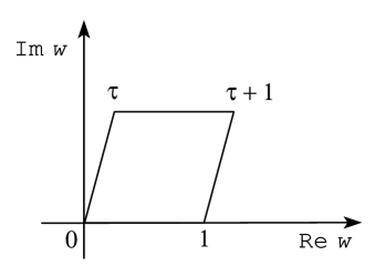
Figure 6: The torus as a quotient of the complex plane.

Although $\tau$ is invariant under infinitesimal diffeomorphisms, it does transform under some “large” transformations. Consider instead of the parallelogram in Fig. 6 defining the torus, the one in Fig. 7a. Obviously, they are equivalent, due to the periodicity conditions (7.4). However, the second one corresponds to a modulus $\tau+1$. We conclude that two tori with moduli differing by 1 are equivalent. Thus, the transformation

$$T\;\;:\;\;\tau\to\tau+1$$ (7.5)

leaves the torus invariant. Consider now another equivalent choice of a parallelogram, that depicted in Fig. 7b, characterized by complex numbers $\tau$ and $\tau+1$. To bring it to the original form (one side on the real axis) and preserve its orientation, we have to scale both sides down by a factor of $\tau+1$. It will then correspond to an equivalent torus with modulus $\tau/(\tau+1)$. We have obtained a second modular transformation

$$TST\;\;:\;\;\tau\to{\tau\over\tau+1}\,.$$ (7.6)

It can be shown that taking products of these transformations generates the full modular group of the torus. A convenient set of generators is given also by $T$ in (7.5) and

$$S\;\;:\;\;\tau\to-{1\over\tau}\;\;\;,\;\;\;S^{2}=1\;\;\;,\;\;\;(ST)^{3}=1\,.$$ (7.7)

The most general transformation is of the form

$$\tau^{\prime}={a\tau+b\over c\tau+d}\;\;\;\leftrightarrow\;\;\;A=\left(\matrix{a&b\cr c&d\cr}\right)\,,$$ (7.8)

where the matrix $A$ has integer entries and determinant 1. Such matrices form the group SL(2,$\hbox{\mybb Z})$. Since changing the sign of the matrix does not affect the modular transformation in (7.8) the modular group is PSL(2,$\rm\hbox{\mybb Z})=SL(2,\hbox{\mybb Z})/\hbox{\mybb Z}_{2}$.

Figure 7: a) The modular transformation $\tau\to\tau+1$. b) The modular transformation $\tau\to\tau/(\tau+1)$.

As mentioned above, the modulus takes values in the upper-half plane ${\cal H}$ ($\tau_{2}\geq 0$), which is the Teichmüller space of the torus. However, to find the moduli space of truly inequivalent tori we have to quotient this with the modular group. It can be shown that the fundamental domain ${\cal F}={\cal H}$/PSL(2,$\hbox{\mybb Z})$ of the modular group is the area contained in between the lines $\tau_{1}=\pm 1/2$ and above the unit circle with center at the origin. It is shown in Fig. 8.

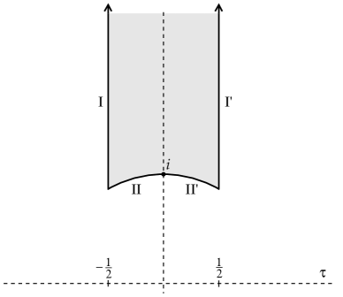
Figure 8: The moduli space of the torus.

There is an interesting construction of the torus starting from the cylinder. Consider a cylinder of length $2\pi\tau_{2}$ and circumference 1. Take one end, rotate it by an angle $2\pi\tau_{1}$ and glue it to the other end. This produces a torus with modulus $\tau=\tau_{1}+i\tau_{2}$. This construction gives a very useful relation between the path integral of a CFT on the torus and a trace over the Hilbert space. First, the propagation along the cylinder is governed by the “Hamiltonian” (transfer matrix) $H=L_{0}^{cyl}+\bar{L}_{0}^{cyl}$. The rotation around the cylinder is implemented by the “momentum” operator $P=L_{0}^{cyl}-\bar{L}_{0}^{cyl}$. Gluing together the two ends gives a trace in the Hilbert space. From (6.7.5)

$$L_{0}^{cyl}=L_{0}-{c\over 24}\;\;\;,\;\;\;\bar{L}_{0}^{cyl}=\bar{L}_{0}-{\bar{c}\over 24}\,,$$ (7.9)

where $L_{0},\bar{L}_{0}$ are the operators on the sphere. Putting everything together, we obtain

$$\int~{}e^{-S} = {\rm Tr}\left[e^{-2\pi\tau_{2}~{}H}~{}e^{2\pi i\tau_{1}~{}P}\right]={\rm Tr}\left[e^{2\pi i\tau L_{0}^{cyl}}~{}e^{-2\pi i\bar{\tau}\bar{L}_{0}^{cyl}}\right]=$$

$$= {\rm Tr}\left[q^{L_{0}-c/24}~{}\bar{q}^{\bar{L}_{0}-\bar{c}/24}\right]\,,$$

where $q=\exp[2\pi i\tau]$. The trace includes also possible continuous parts of the spectrum. This is a very useful relation and also provides the correct normalization of the path integral.

7.1 Compact scalars

In section 6.4 we have described the CFT of a non-compact real scalar field. Here we will consider a compact scalar field $X$ taking values on a circle of radius $R$. Consequently, the values $X$ and $X+2\pi mR$, $m\in Z$ will be considered equivalent.

We will first evaluate the path integral of the theory on the torus. The action is

$$S = \frac{1}{4\pi}\int d^{2}\sigma\sqrt{g}~{}g^{ij}\partial_{i}X{\partial}_{j}X$$ (7.1.1)

$$= \frac{1}{4\pi}\int_{0}^{1}d\sigma_{1}\int_{0}^{1}d\sigma_{2}{1\over\tau_{2}}|\tau\partial_{1}X-\partial_{2}X|^{2}$$

$$= -{1\over 4\pi}\int d^{2}\sigma~{}X\hbox{{$\sqcup$}\hbox to0.0pt{\hss$\sqcap$}}~{}X\,,$$

where the Laplacian is given by

$$\hbox{{$\sqcup$}\hbox to0.0pt{\hss$\sqcap$}}={1\over\tau_{2}}|\tau\partial_{1}-\partial_{2}|^{2}\,.$$ (7.1.2)

We wish to evaluate the path integral

$$Z(R)=\int~{}DX~{}e^{-S}$$ (7.1.3)

on the torus. As usual, we will have to find the classical solutions of finite action (instantons) and calculate the fluctuations around them. The field $X$ should be periodic on the torus and is a map from the torus (topologically $S^{1}\times S^{1}$) to the circle $S^{1}$. Such maps are classified by two integers that specify how many times $X$ winds around the two cycles of the torus. The equation of motion $\hbox{{$\sqcup$}\hbox to0.0pt{\hss$\sqcap$}}X=0$ has the following instanton solutions

$$X_{class}=2\pi R(n\sigma_{1}+m\sigma_{2})\;\;\;,\;\;\;m,n\in\hbox{\mybb Z}\;\;\;.$$ (7.1.4)

They have the correct periodicity properties

$$X_{class}(\sigma_{1}+1,\sigma_{2})=X(\sigma_{1},\sigma_{2})+2\pi nR\;\;,\;\;X_{class}(\sigma_{1},\sigma_{2}+1)=X(\sigma_{1},\sigma_{2})+2\pi mR\;,$$ (7.1.5)

and the following classical action

$$S_{m,n}={\pi R^{2}\over\tau_{2}}|m-n\tau|^{2}\,.$$ (7.1.6)

Thus, we can separate $X=X_{class}+\chi$, and the path integral can be written as

$$Z(R) = \sum_{m,n\in\hbox{\mybb Z}}\int~{}D\chi~{}e^{-S_{m,n}-S(\chi)}$$ (7.1.7)

$$= \sum_{m,n\in\hbox{\mybb Z}}e^{-S_{m,n}}~{}\int~{}D\chi~{}e^{-S(\chi)}\,.$$

What remains to be done is the path integral over $\chi$. There is always the constant zero mode that we can separate, $\chi(\sigma_{1},\sigma_{2})=\chi_{0}+\delta\chi(\sigma_{1},\sigma_{2})$, with $0\leq\chi_{0}\leq 2\pi R$. The field $\delta\chi$ can be expanded in the eigenfunctions of the Laplacian

$$\hbox{{$\sqcup$}\hbox to0.0pt{\hss$\sqcap$}}\psi_{i}=-\lambda_{i}~{}\psi_{i}\,.$$ (7.1.8)

It is not difficult to see that these eigenfunctions are

$$\psi_{m_{1},m_{2}}=e^{2\pi i(m_{1}\sigma_{1}+m_{2}\sigma_{2})}\;\;\;,\;\;\;\lambda_{m_{1},m_{2}}={4\pi^{2}\over\tau_{2}}|m_{1}\tau-m_{2}|^{2}\,.$$ (7.1.9)

The eigenfunctions satisfy

$$\int d^{2}\sigma~{}\psi_{m_{1},m_{2}}\psi_{n_{1},n_{2}}=\delta_{m_{1}+n_{1},0}\delta_{m_{2}+n_{2},0}\,,$$ (7.1.10)

so we expand

$$\delta\chi={\sum_{m_{1},m_{2}\in{\hbox{\mybb Z}}}}^{\prime}A_{m_{1},m_{2}}\psi_{m_{1},m_{2}}\,,$$ (7.1.11)

where the prime implies omission of the constant mode $(m_{1},m_{2})=(0,0)$. Reality implies $A^{*}_{m_{1},m_{2}}=A_{-m_{1},-m_{2}}$. The action becomes

$$S(\chi)={1\over 4\pi}{\sum_{m_{1},m_{2}}}^{{}^{\prime}}~{}\lambda_{m_{1},m_{2}}~{}|A_{m_{1},m_{2}}|^{2}\,.$$ (7.1.12)

We can specify the measure from

$$\|\delta X\|=\int d^{2}\sigma\sqrt{\mbox{det}G}(d\chi)^{2}={\sum_{m_{1},m_{2}}}^{{}^{\prime}}|dA_{m_{1},m_{2}}|^{2}$$ (7.1.13)

to be

$$\int~{}D\chi=\int_{0}^{2\pi R}d\chi_{0}~{}{\prod_{m_{1},m_{2}}}^{{}^{\prime}}{dA_{m_{1},m_{2}}\over 2\pi}\,.$$ (7.1.14)

Putting everything together we obtain

$$\int D\chi e^{-S(\chi)}={2\pi R\over{\prod_{m_{1},m_{2}}}^{{}^{\prime}}\lambda_{m_{1},m_{2}}^{1/2}}={2\pi R\over\sqrt{{\rm det}^{\prime}\hbox{{$\sqcup$}\hbox to0.0pt{\hss$\sqcap$}}}}\,.$$ (7.1.15)

Using the explicit form of the eigenvalues, the determinant of the Laplacian can be calculated using a $\zeta$-function regularization [13],

$${\rm det}^{\prime}\hbox{{$\sqcup$}\hbox to0.0pt{\hss$\sqcap$}}=4\pi^{2}\tau_{2}\eta^{2}(\tau)\bar{\eta}^{2}(\bar{\tau})\,,$$ (7.1.16)

where $\eta$ is the Dedekind function defined in (A.10). Collecting all terms in (7.1.7) we obtain

$$Z(R)={R\over\sqrt{\tau_{2}}|\eta|^{2}}\sum_{m,n\in Z}e^{-{\pi R^{2}\over\tau_{2}}|m-n\tau|^{2}}\,.$$ (7.1.17)

This is the Lagrangian form of the partition function. We have mentioned in the previous chapter that the partition function on the torus can also be written in Hamiltonian form as in (7). To do this we have to perform a Poisson resummation (see appendix A) on the integer $m$. We obtain

$$Z(R)=\sum_{m,n\in\hbox{\mybb Z}}~{}{q^{{P^{2}_{L}\over 2}}~{}\bar{q}^{P^{2}_{R}\over 2}\over\eta\bar{\eta}}$$ (7.1.18)

with

$$P_{L}={1\over\sqrt{2}}\left({m\over R}+nR\right)\;\;\;,\;\;\;P_{R}={1\over\sqrt{2}}\left({m\over R}-nR\right)\,\,.$$ (7.1.19)

This is in the form (7) and from it we can read off the spectrum of conformal weights and multiplicities of the theory. Before we do this, however, let us return to the sphere and discuss the current algebra structure of the theory. As in section 6.4 there is a holomorphic and anti-holomorphic U(1) current:

$$J(z)=i\partial X\;\;\;,\;\;\;\bar{J}(\bar{z})=i\bar{\partial}X$$ (7.1.20)

satisfying the U(1) current algebra

$$J(z)J(w)={1\over(z-w)^{2}}+{\rm finite}\;\;,\;\;\bar{J}(\bar{z})\bar{J}(\bar{w})={1\over(\bar{z}-\bar{w})^{2}}+{\rm finite}\,.$$ (7.1.21)

We can write the stress-tensor in the affine-Sugawara form

$$T(z)=-{1\over 2}(\partial X)^{2}={1\over 2}:J^{2}:\;\;\;,\;\;\;\bar{T}(\bar{z})=-{1\over 2}(\bar{\partial}X)^{2}={1\over 2}:\bar{J}^{2}:\,.$$ (7.1.22)

The spectrum can be decomposed into affine HW representations as discussed in section 6.10. An affine primary field is specified by its charges $Q_{L}$ and $Q_{R}$ under the left- and right-moving current algebras. From (7.1.22) we obtain that its conformal weights are given by

$$\Delta={1\over 2}Q_{L}^{2}\;\;\;,\;\;\;\bar{\Delta}={1\over 2}Q_{R}^{2}\,.$$ (7.1.23)

The rest of the representation is constructed by acting on the affine primary state with the negative current modes $J_{-n}$ and $\bar{J}_{-n}$. We can easily compute the character of such a representation ($c=\bar{c}=1$):

$$\chi_{Q_{L},Q_{R}}(q,\bar{q})={\rm Tr}[q^{L_{0}-1/24}\bar{q}^{\bar{L}_{0}-1/24}]={q^{Q_{L}^{2}/2}~{}\bar{q}^{Q_{R}^{2}/2}\over\eta\bar{\eta}}\,.$$ (7.1.24)

A comparison with (7.1.18) shows that the spectrum contains an infinite number of affine U(1) representations labeled by $m,n$ with $Q_{L}=P_{L}$ and $Q_{R}=P_{R}$. For $m=n=0$ we have the vacuum representation whose HW state is the standard vacuum. The other HW states, labeled by $m,n$ satisfy

$$J_{0}|m,n\rangle=P_{L}~{}|m,n\rangle\;\;\;,\;\;\;\bar{J}_{0}|m,n\rangle=P_{R}~{}|m,n\rangle\,\,.$$ (7.1.25)

In the operator picture, they are created out of the vacuum by the vertex operators (we split $X(z,\bar{z})\sim X(z)+\bar{X}(\bar{z})$ as usual):

$$V_{m,n}=:\exp[i~{}p_{L}~{}X+i~{}p_{R}~{}\bar{X}]:\,,$$ (7.1.26)

$$J(z)V_{m,n}(w,\bar{w}) = p_{L}{V_{m,n}(w,\bar{w})\over z-w}+\dots\;,$$

$$\bar{J}(\bar{z})V_{m,n}(w,\bar{w}) = p_{R}{V_{m,n}(w,\bar{w})\over\bar{z}-\bar{w}}+\dots\,.$$ (7.1.27)

Their correlators are again given by the Gaussian formula

$$\left\langle~{}\prod_{i=1}^{N}~{}V_{m_{i},n_{i}}(z_{i},\bar{z}_{i})~{}\right\rangle=\prod_{i<j}^{N}~{}z_{ij}^{p^{i}_{L}p^{j}_{L}}~{}\bar{z}_{ij}^{p^{i}_{R}p^{j}_{R}}\,,$$ (7.1.28)

where as usual $z_{ij}=z_{i}-z_{j}$. Using the Gaussian formula

$$:e^{ia\phi(z)}::e^{ib\phi(w)}: = (z-w)^{ab}:e^{ia\phi(z)+ib\phi(w)}:$$ (7.1.29)

$$= (z-w)^{ab}\left[:e^{i(a+b)\phi(w)}:+{\cal O}(z-w)\right]\;,$$

we obtain the following OPE rule for U(1) representations

$$[V_{m_{1},n_{1}}]\cdot[V_{m_{2},n_{2}}]\sim[V_{m_{1}+m_{2},n_{1}+n_{2}}]\,,$$ (7.1.30)

compatible with U(1) charge conservation. Under the $\rm U(1)_{L}\times U(1)_{R}$ transformation $e^{i\theta_{L}+i\theta_{R}}$ the oscillators are invariant but the states $|m,n\rangle$ pick up a phase $e^{i(m+n)\theta_{L}+i(m-n)\theta_{R}}$.

In the canonical representation, the momentum operator is taking values $m/R$ as required by the usual (point-particle) quantum mechanical quantization condition on a circle of radius $R$. The existence of the extra spatial dimension of the string allows for the possibility of $X$ winding around the circle $n$ times. This is precisely the interpretation of the integer $n$ in (7.1.19). It has no point-particle (one-dimensional) analogue.

In a CFT, there is a special class of operators, known as marginal operators, with $(\Delta,\bar{\Delta})=(1,1)$. For such an operator $\phi_{1,1}$, the density $\phi_{1,1}dzd\bar{z}$ is conformally invariant. If we perturb our action by $g\int\phi_{1,1}$ we would expect that the theory remains conformally invariant. There are subtleties in the quantum theory, however (short distance singularities) which sometimes spoil conformal invariance. When conformal invariance persists, we call $\phi_{1,1}$ exactly marginal. In this way, perturbing by $\phi_{1,1}$ we obtain a continuous family of CFTs parametrized by the coupling $g$. The central charge cannot change during a marginal perturbation.

In our present example we have an occurrence of this phenomenon. There is a (1,1) operator namely $\phi=\partial X\bar{\partial}X=J\bar{J}$. By adding this to the action (7.1.1), it is easy to see that the effect of the perturbation is to change the effective radius $R$. The theory, being again a free field theory, remains conformally invariant. In this case the operation seems trivial, however, marginal operators exist in more complicated CFTs.

Finally let us go back to the torus and take another look at the partition function. For string theory purposes we would like it to be invariant under the full diffeomorphism group. In particular it should be invariant under the large transformations, namely the modular transformations. This is important in string theory since modular invariance is at the very heart of finiteness of string theory and is essential for the cancelation of spacetime anomalies.

It suffices to prove invariance under the two generating transformations $T$ and $S$, since these generate the modular group. We will use the Lagrangian representation of the partition function (7.1.17). It is not difficult to verify, using the formulae of appendix A, that $\sqrt{\tau_{2}}\eta\bar{\eta}$ is separately modular-invariant. Thus, we only need to consider the instanton sum. Under $\tau\to\tau+1$ we can change the summation $(m,n)\to(m+n,n)$, and the full sum is invariant. Under $\tau\to-1/\tau$ we can again change the summation $(m,n)\to(-n,m)$ and again the sum is invariant. We conclude that the torus partition function of the compact boson is modular-invariant. It is interesting to note that invariance under the $T$ transformation in the Hamiltonian representation (7) implies

$$\Delta-\bar{\Delta}-{c-\bar{c}\over 24}={\rm integer}$$ (7.1.31)

for the whole spectrum. In particular, for the vacuum state $\Delta=\bar{\Delta}=0$, it implies that $c-\bar{c}=0~{}$mod$~{}(24)$. In our case $c=\bar{c}=1$ and from (7.1.19), (7.1.23) $P^{2}_{L}/2-P^{2}_{R}/2=mn\in\hbox{\mybb Z}$.

Another comment concerns the partition function on the torus of a non-compact boson. This can be obtained by taking the limit $R\to\infty$. We expect that the partition function in this limit diverges like the volume of our space, so we have to divide first by the volume. The free energy per unit volume is finite. From (7) we note that as $R$ gets large, the only term that is not exponentially suppressed is the one with $m=n=0$, so

$$\lim_{R\to\infty}{Z(R)\over R}={1\over\sqrt{\tau_{2}}\eta\bar{\eta}}\,.$$ (7.1.32)

Before we proceed, we will derive the torus propagator for the boson. It can be directly written in terms of the non-zero eigenvalues and the associated eigenfunctions of the Laplacian:

$$\Delta(\sigma_{1},\sigma_{2})\equiv\langle\delta\chi(\sigma_{1},\sigma_{2})\delta\chi(0,0)\rangle=-{\sum_{m,n}}^{\prime}{1\over|m\tau-n|^{2}}e^{2\pi i(m\sigma_{1}+n\sigma_{2})}\,.$$ (7.1.33)

The sum is conditionally convergent and has to be regularized using $\zeta$-function regularization. We obtain

$$\hbox{{$\sqcup$}\hbox to0.0pt{\hss$\sqcap$}}~{}\Delta(\sigma_{1},\sigma_{2})={4\pi^{2}\over\tau_{2}}\left[\delta(\sigma_{1})\delta(\sigma_{2})-1\right]\,,$$ (7.1.34)

so that the integral over the torus gives zero, in accordance with the fact that we have omitted the zero mode. It can also be expressed in complex coordinates in terms of $\vartheta$-functions as

$$\Delta(\sigma_{1},\sigma_{2})=-\log G(z,\bar{z})\;\;\;,\;\;\;G=e^{-2\pi{Imz^{2}\over\tau_{2}}}{}~{}\left|{\vartheta_{1}(z)\over\vartheta_{1}^{\prime}(0)}\right|^{2}\,\,.$$ (7.1.35)

The above discussion can easily be generalized to the case of $N$ free compact scalar fields $X^{i}$, $i=1,2,\dots,N$. We will take them to have values in $[0,2\pi]$. They parametrize an $N$-dimensional torus. The most general quadratic action is

$$S={1\over 4\pi}\int d^{2}\sigma\sqrt{\mbox{det}~{}g}g^{ab}G_{ij}\partial_{a}X^{i}\partial_{b}X^{j}+{1\over 4\pi}\int d^{2}\sigma\epsilon^{ab}B_{ij}\partial_{a}X^{i}\partial_{b}X^{j}\;,$$ (7.1.36)

where $g_{ab}$ is the torus metric (7.1), $\epsilon^{ab}$ is the usual $\epsilon$-symbol, $\epsilon^{12}=1$; $G_{ij}$ is a constant symmetric positive-definite matrix that plays the role of metric in the space of the $X^{i}$ (target-space torus). The constant matrix $B_{ij}$ is antisymmetric. It is the analogue of the $\theta$-term in four-dimensional gauge theories.

An analogous calculation of the path integral produces

$$\hbox{\mybb Z}_{\mbox{\tiny d,d}}(G,B)=\frac{\sqrt{\mbox{det}~{}G}}{(\sqrt{\tau_{2}}\eta\bar{\eta})^{N}}\sum_{\vec{m},\vec{n}}e^{-\frac{\pi(G_{ij}+B_{ij})}{\tau_{2}}(m_{i}+n_{i}\tau)(m_{j}+n_{j}\bar{\tau})}\,.$$ (7.1.37)

This partition function reduces for N=1, $G=R^{2}$, $B=0$ to (7). Using a multiple Poisson resummation on the $m_{i}$, it can be transformed in the Hamiltonian representation:

$$\hbox{\mybb Z}_{\mbox{\tiny d,d}}(G,B)={\Gamma_{d,d}(G,B)\over\eta^{d}\bar{\eta}^{d}}=\sum_{\vec{m},\vec{n}\in\hbox{\mybb Z}^{N}}{q^{{1\over 2}P_{L}^{2}}~{}\bar{q}^{{1\over 2}P_{R}^{2}}\over\eta^{N}\bar{\eta}^{N}}\,,$$ (7.1.38)

where

$$P_{L,R}^{2}\equiv P^{i}_{L,R}~{}G_{ij}P^{j}_{L,R}\,,$$ (7.1.39)

$$P^{i}_{L}={G^{ij}\over\sqrt{2}}(m_{j}+(B_{jk}+G_{jk})n_{k})\;\;\;,\;\;\;P^{i}_{R}={G^{ij}\over\sqrt{2}}(m_{j}+(B_{jk}-G_{jk})n_{k})\,.$$ (7.1.40)

The theory has a left-moving and a right-moving U(1)^N current algebra generated by the currents

$$J^{i}(z)=i\partial X^{i}\;\;\;,\;\;\;\bar{J}^{i}=i\bar{\partial}X^{i}\,\,,$$ (7.1.41)

$$J^{i}(z)J^{j}(w)={G^{ij}\over(z-w)^{2}}+\dots$$ (7.1.42)

and similarly for $\bar{J}^{i}$. The stress-tensor is again of the affine-Sugawara form

$$T(z)=-{1\over 2}G_{ij}\partial X^{i}\partial X^{j}={1\over 2}G_{ij}:J^{i}J^{j}:\,.$$ (7.1.43)

Affine primaries are characterized by charges $Q^{i}_{L,R}$ and

$$\Delta={1\over 2}G_{ij}Q^{i}_{L}Q^{j}_{L}\;\;\;,\;\;\;\bar{\Delta}={1\over 2}G_{ij}Q^{i}_{R}Q^{j}_{R}\,.$$ (7.1.44)

Comparing this with (7.1.38) we obtain $Q^{i}_{L,R}=P^{i}_{L,R}$.

It can be shown that the partition function (7.1.38) is modular-invariant.

7.2 Enhanced symmetry and the string Higgs effect

Something special happens to the CFT of the single compact boson when the radius is $R=1$. The conformal weights of the primaries are now given by

$$\Delta={1\over 4}(m+n)^{2}\;\;\;,\;\;\;\bar{\Delta}={1\over 4}(m-n)^{2}\,.$$ (7.2.1)

Notice that the two states with $m=n=\pm 1$ are (1,0) operators. For generic $R$ the only (1,0) (chiral) operator is the U(1) current $J(z)=i\partial X$. Now we have two more. We expect that the current algebra becomes larger if we also include these operators. Similarly, the states with $m=-n=\pm 1$ are (0,1) operators and the right-moving current algebra is also enhanced. We will discuss only the left-moving part, since the right-moving part behaves in a similar way. The two operators that become (1,0) can be written as vertex operators (7.1.26)

$$J^{\pm}(z)={1\over\sqrt{2}}:e^{\pm i\sqrt{2}X(z)}:\,.$$ (7.2.2)

Define also

$$J^{3}(z)={1\over\sqrt{2}}J(z)={i\over\sqrt{2}}\partial X(z)\,.$$ (7.2.3)

They satisfy the following OPEs, which can be computed directly using $\langle X(z)X(0)\rangle=-\log z$,

$$J^{3}(z)J^{\pm}(w)=\pm{J^{\pm}(w)\over z-w}+\dots\;\;\;,\;\;\;J^{+}(z)J^{+}(w)=\dots\;\;,$$

$$J^{-}(z)J^{-}(w)=\dots\,,$$ (7.2.4)

$$J^{+}(z)J^{-}(w)={1/2\over(z-w)^{2}}+{J^{3}(w)\over z-w}+\dots\;\;,$$

$$J^{3}(z)J^{3}(w)={1/2\over(z-w)^{2}}+\dots\,.$$ (7.2.5)

It is not difficult to realize that this is the SU(2) current algebra with level $k=1$. This is not too surprising, since the central charge of $\rm SU(2)_{k}$ is given by (6.10.6) to be $c=3k/(k+2)$. It indeed becomes $c=1$ when $k=1$. This realization of current algebra at level 1 in terms of free bosons is known as the Halpern-Frenkel-Kac-Segal construction.

We have seen before that $\rm SU(2)_{1}$ has two integrable affine representations, the vacuum representation with $j=0$ and the $j=1/2$ representation with conformal weight $\Delta=1/4$ (from (6.10.9)). The primary state of the $j=0$ representation is the vacuum. The primary operators of the $j=1/2$ representation transform as a two-component spinor of $\rm SU(2)_{L}$ and a two-component spinor of $\rm SU(2)_{R}$ with conformal weights (1/4,1/4). They are represented by the four vertex operators $V_{m,n}$ with $(m,n)=(0,\pm 1)$ and $(\pm 1,0)$. They have the correct conformal weight and OPEs with the currents (7.2.2).

This phenomenon generalizes to the N-dimensional toroidal models. The U(1) charges $p^{i}_{L,R}$ take values on an N-dimensional lattice that depends on $G_{ij},B_{ij}$. For special values of G,B this lattice coincides with the root lattice of a Lie group $G$ with rank N. Then some vertex operators become extra chiral currents and along with the $N$ abelian currents $J^{i}$ form an affine $G$ algebra at level $k=1$.

When the toroidal CFT acquires enhanced current algebra symmetry then the associated string theory acquires enhanced gauge symmetry. Consider the bosonic string with one of the 26 dimensions (say $X^{25}$) compactified on a circle of radius $R$. Then the massless states are again similar, but with a slightly different interpretation. There are now 25 non-compact dimensions, so we have 25-dimensional Lorentz invariance. The massless states are

$$a^{\mu}_{-1}\bar{a}^{\nu}_{-1}|0\rangle\;\;\;,\;\;\;a^{\mu}_{-1}\bar{a}^{25}_{-1}|0\rangle\;\;\;,\;\;\;a^{25}_{-1}\bar{a}^{\mu}_{-1}|0\rangle\;\;\;,\;\;\;a^{25}_{-1}\bar{a}^{25}_{-1}|0\rangle\,,$$ (7.2.6)

which are the graviton, antisymmetric tensor, dilaton, two U(1) gauge fields and a scalar. Note that the scalar state is generated by $\partial X^{25}\bar{\partial}X^{25}$, which is the perturbation that changes the radius. Thus, the expectation value of the scalar is the radius $R$. There are other massive states, among them

$$|A^{\pm}_{\mu}\rangle=\bar{a}^{\mu}|m=\pm 1,n=\pm 1\rangle\,,$$ (7.2.7)

which are massive vectors with mass $m^{2}=(R-1/R)^{2}/4$ and

$$|\bar{A}^{\pm}_{\mu}\rangle=a^{\mu}|m=\pm 1,n=\mp 1\rangle$$ (7.2.8)

with the same mass as above. As we vary $R$ the mass changes, and at $R=1$ they become massless. At that point, the string theory acquires an SU(2)$\times$SU(2) gauge symmetry. Moving away from $R=1$, SU(2)$\times$SU(2) gauge symmetry is spontaneously broken to U(1)$\times$U(1). This is the usual Higgs effect and the scalar whose expectation value is the radius plays the role of the Higgs scalar (although there is no potential here).

7.3 T-duality

We now return to the example of a single scalar, compactified on a circle of radius $R$, discussed in the previous section. As we have seen the primaries have

$$H=L_{0}+\bar{L}_{0}={1\over 2}\left({m^{2}\over R^{2}}+n^{2}R^{2}\right)\;\;\;,\;\;\;P=L_{0}-\bar{L}_{0}=mn\,.$$ (7.3.1)

It is obvious that the above spectrum is invariant under

$$R\to{1\over R}\;\;\;,\;\;\;m\leftrightarrow n\,.$$ (7.3.2)

This corresponds to the following transformation of the U(1) charges

$$P_{L}\to P_{L}\;\;\;,\;\;\;P_{R}\to-P_{R}\,.$$ (7.3.3)

Only the right charge changes sign. The action on the respective currents is analogous

$$J(z)\to J(z)\;\;\;,\;\;\;\bar{J}(\bar{z})\to-\bar{J}(\bar{z})\,.$$ (7.3.4)

It can be easily checked that not only the spectrum but also the interactions respect this property. This is a peculiar property since it implies that a CFT cannot distinguish a circle of radius $R$ from another of radius $1/R$. This is, strictly speaking, not a symmetry of the two-dimensional theory. It states that two a priori different theories are in fact equivalent. However, in the context of string theory it will become a true symmetry and is known under the name $T$-duality. Notice that the presence of winding modes is essential for the presence of $T$-duality. Therefore it can appear in string theory but not in point-particle field theory.

There is an interesting interpretation of $T$-duality in string theory. We start from the CFT with $R=1$. We have seen that at this point there is an enhanced symmetry $\rm SU(2)_{L}\times SU(2)_{R}$. Then, at this point, the duality transformation (7.3.4) is an $\rm SU(2)_{R}$ Weyl transformation, which is an obvious symmetry of the CFT. This explains the self-duality at $R=1$. Move now infinitesimally away from $R=1$ by perturbing the CFT with the marginal operator $\epsilon\int J^{3}\bar{J}^{3}=\epsilon\int\partial X\bar{\partial}X$. Because of the self-duality of the unperturbed theory, the $\epsilon$ perturbation and $-\epsilon$ perturbation give identical theories. This is the infinitesimal version of $R\to 1/R$ duality around $R=1$. We can further extend this duality on the whole line. In this sense the duality is a consequence of SU(2) symmetry at $R=1$ and the duality transformation is an $\rm SU(2)_{R}$ transformation. Consider again the bosonic string with one dimension compactified. At $R=1$ the $\rm SU(2)_{L}$ transformation is a gauge transformation. Away from $R=1$ the gauge symmetry is broken and the duality symmetry is a discrete remnant of the original gauge symmetry.

We can generalize the $T$-duality symmetry to the N-dimensional toroidal models; here the duality transformations form an infinite discrete group, unlike the one-dimensional case where the group was $Z_{2}$.

First observe that the partition function (7.1.37) is invariant under shifts of $B_{ij}$ by any antisymmetric matrix with integer entries. Also by construction the theory is invariant under $GL(N)$ rotations of the scalars $G_{ij}$ and $B_{ij}$. However, since the rotations also act on $m_{i},n_{i}$ they have to rotate them back to integers. The $GL(N)$ matrix must have integer entries and such matrices form the discrete group $GL(N,\hbox{\mybb Z})$. Finally there are transformations such as the radius inversion, which leave the spectrum invariant. Together, all of these transformations combine into an infinite discrete group O(N,N,$\hbox{\mybb Z})$. It is described by $2N\times 2N$ integer-valued matrices of the form

$$\Omega=\left(\begin{array}[]{cc}A&B\\ C&D\end{array}\right)\,,$$ (7.3.5)

where $A,B,C,D$ are $N\times N$ matrices. Define also the O(N,N)-invariant metric

$$L=\left(\matrix{0&{\bf 1}_{N}\cr{\bf 1}_{N}&0\cr}\right)\,,$$ (7.3.6)

where ${\bf 1}_{N}$ is the $N$-dimensional unit matrix. $\Omega$ belongs to O(N,N,$\hbox{\mybb Z})$ if it has integer entries and satisfies

$$\Omega^{T}~{}L~{}\Omega=L\,.$$ (7.3.7)

Define $E_{ij}=G_{ij}+B_{ij}$. Then the duality transformations are

$$E\rightarrow(AE+B)(CE+D)^{-1}\;\;\;,\;\;\;\left(\begin{array}[]{c}\vec{m}\\ \vec{n}\end{array}\right)\rightarrow\Omega\left(\begin{array}[]{c}\vec{m}\\ \vec{n}\end{array}\right)\,.$$ (7.3.8)

In the special (but useful) case N=2 we can parametrize

$$G_{ij}={T_{2}\over U_{2}}\left(\matrix{1&U_{1}\cr U_{1}&U_{1}^{2}+U_{2}^{2}\cr}\right)\;\;\;,\;\;\;B_{ij}=\left(\matrix{0&T_{1}\cr-T_{1}&0\cr}\right)\;,$$ (7.3.9)

with $T_{2},U_{2}\geq 0$. Defining the complex parameters $T=T_{1}+iT_{2}$, $U=U_{1}+iU_{2}$, the lattice sum (7.1.38) becomes

$$\Gamma_{2,2}(T,U)=\sum_{\vec{m},\vec{n}}\exp\left[-{\pi\tau_{2}\over T_{2}U_{2}}|-m_{1}U+m_{2}+T(n_{1}+Un_{2})|^{2}+\right.$$

$$\left.\rule[-6.45831pt]{0.0pt}{17.22217pt}+2\pi i\tau(m_{1}n_{1}+m_{2}n_{2})\right]\,.$$ (7.3.10)

The duality group O(2,2,$\hbox{\mybb Z})$ acts on $T$ and $U$ with independent PSL(2,$\hbox{\mybb Z})$ transformations (7.8) as well as with the exchange $T\leftrightarrow U$.

$T$-duality can be generalized to $s$-models that have a curved target space. For a more detailed discussion, see [25].

7.4 Free fermions on the torus

In section 6.11 we have analyzed the CFT of $N$ free Majorana-Weyl fermions. We will now consider the partition function of this theory on the torus. The action was given in (6.11.1). To do the path integral, we have to choose boundary conditions for the fermions around the two cycles of the torus. For each cycle we have the choice between periodic and antiperiodic boundary conditions. In total we have four possible sectors. The fermionic path integral will give a power of the fermionic determinant defined with the appropriate boundary conditions (also known as spin-structures).

$$\int e^{-S}=({\rm det}~{}\partial)^{N/2}\,.$$ (7.4.1)

This can be computed by finding the appropriate eigenvalues and taking the $\zeta$-regularized product. We will first consider antiperiodic boundary conditions on both cycles (A,A). Then the eigenvalues are

$$\lambda_{AA}\sim\left(\left(m_{1}+{1\over 2}\right)\tau+\left(m_{2}+{1\over 2}\right)\right)\;\;\;,\;\;\;m_{1,2}\in\hbox{\mybb Z}\,.$$ (7.4.2)

A calculation of the regularized product gives

$$({\rm det}~{}\partial)_{AA}={\vartheta_{3}(\tau)\over\eta(\tau)}\,.$$ (7.4.3)

For (A,P) boundary conditions we obtain

$$\lambda_{AP}\sim\left(\left(m_{1}+{1\over 2}\right)\tau+m_{2}\right)\;\;\;,\;\;\;m_{1,2}\in\hbox{\mybb Z}\,,$$ (7.4.4)

$$({\rm det}~{}\partial)_{AP}={\vartheta_{4}(\tau)\over\eta(\tau)}\,.$$ (7.4.5)

For (P,A) boundary conditions we have

$$\lambda_{PA}\sim\left(m_{1}\tau+\left(m_{2}+{1\over 2}\right)\right)\;\;\;,\;\;\;m_{1,2}\in\hbox{\mybb Z}\,,$$ (7.4.6)

$$({\rm det}~{}\partial)_{PA}={\vartheta_{2}(\tau)\over\eta(\tau)}\,.$$ (7.4.7)

Finally for (P,P) boundary conditions the determinant vanishes, since these boundary conditions now allow zero modes. By coupling to constant gauge fields (which act as sources for the zero modes) it can be seen that the determinant here is proportional to $\vartheta_{1}(\tau)$, which indeed is identically zero.

We can summarize the above results as follows. Let $a=0,1$ indicate A,P boundary conditions respectively around the first cycle and $b=0,1$ indicate A,P around the second. Then

$$(\det\partial)[^{a}_{b}]={\vartheta[^{a}_{b}](\tau)\over\eta(\tau)}\,.$$ (7.4.8)

The (P,P) spin-structure is known as the odd spin-structure, the rest as even spin-structures. From appendix A we can see that modular transformations permute the various boundary conditions since they permute the various cycles. To construct something that is modular-invariant, we will have to sum over all boundary conditions. Including also the right-moving fermions we can write the full partition function as

$$Z_{N}^{\rm fermionic}={\textstyle{1\over 2}}\sum_{a,b=0}^{1}\left|{\vartheta[^{a}_{b}]\over\eta}\right|^{N}\,.$$ (7.4.9)

It can be checked directly that it is modular-invariant. To expose the spectrum, we can express the partition function in terms of the characters (6.11.28), (6.11.29), (6.11.42), (6.11.43) as

$$Z_{N}^{\rm fermionic}=|\chi_{0}|^{2}+|\chi_{V}|^{2}+|\chi_{S}|^{2}+|\chi_{C}|^{2}\,,$$ (7.4.10)

from which we see that all $\rm O(N)_{1}$ integrable representations participate.

The two-point functions of the fermions in the even spin-structures can be fixed in terms of their pole structure and transformation properties under modular transformations. They are given by the Szegö kernel

$$\langle\psi^{i}(z)\psi^{j}(0)\rangle=\delta^{ij}~{}S[^{a}_{b}](z)\;\;\;,\;\;\;S[^{a}_{b}](z)={\vartheta[^{a}_{b}](z)\vartheta_{1}^{\prime}(0)\over\vartheta_{1}(z)\vartheta[^{a}_{b}](0)}\,.$$ (7.4.11)

We will also discuss the zero modes in the odd spin-structure further. Each real fermion has a zero mode, and the path integral vanishes. The first non-zero correlation function must contain $N$ fermions so that they soak up all the zero modes. The integral over the zero modes gives a completely antisymmetric tensor, which we normalize to the invariant $\epsilon$-tensor. The rest of the contribution is given by the partition function in the absence of zero modes. Since the oscillators are integrally moded and since there is a $(-1)^{F}$ insertion, the non-zero mode contribution is

$$q^{-N/24}\prod_{n=1}^{\infty}(1-q^{n})^{N}=\eta^{N}=\left[{1\over 2\pi}{\partial_{v}\vartheta_{1}(v)|_{v=0}\over\eta}\right]^{N/2}\,.$$ (7.4.12)

Thus,

$$\left\langle\prod_{k=1}^{N}\psi^{i_{k}}(z_{k})\right\rangle_{\rm odd}=\epsilon^{i_{1},\dots,i_{N}}~{}\eta^{N}\,.$$ (7.4.13)

7.5 Bosonization

Consider two Majorana-Weyl fermions $\psi^{i}(z)$ with

$$\psi^{i}(z)\psi^{j}(w)={\delta^{ij}\over z-w}+\dots\,.$$ (7.5.1)

We can change basis to

$$\psi={1\over\sqrt{2}}(\psi^{1}+i\psi^{2})\;\;\;,\;\;\;\bar{\psi}={1\over\sqrt{2}}(\psi^{1}-i\psi^{2})\,.$$ (7.5.2)

The theory contains a U(1) current algebra generated by the (1,0) current

$$J(z)=:\psi\bar{\psi}:\;\;\;,\;\;\;J(z)J(w)={1\over(z-w)^{2}}+\dots\,,$$ (7.5.3)

$$J(z)\psi(w)={\psi(w)\over z-w}+\dots\;\;\;,\;\;\;J(z)\bar{\psi}(w)=-{\bar{\psi}(w)\over z-w}+\dots\,.$$ (7.5.4)

Equation (7.5.4) states that $\psi,\bar{\psi}$ are affine primaries with charges 1 and $-1$. The stress-tensor is

$$T(z)=-{1\over 2}:\psi^{i}\partial\psi^{i}:={1\over 2}:J^{2}:\,.$$ (7.5.5)

It has central charge $c=1$.

We can represent the same operator algebra using a single chiral boson $X(z)$. Namely

$$J(z)=i\partial X\;\;\;,\;\;\;\psi=:e^{iX}:\;\;\;,\;\;\;\bar{\psi}=:e^{-iX}:\,.$$ (7.5.6)

Exercise: Verify that the above definitions reproduce the same OPEs as in the fermionic theory.

Moreover, applying these definitions to (7.5.5) they produce the correct stress-tensor of the scalar, namely $T=-{\textstyle{1\over 2}}:\partial X^{2}:$. This chiral operator construction suggests that two Majorana-Weyl fermions and a chiral boson might give equivalent theories. However, the full theories contain also right-moving parts. When included, we are considering on the one hand a Dirac fermion and on the other a scalar. For the scalar theory, however, we have to specify the radius $R$. To do this we start from the partition function of the torus for a Dirac fermion (7.4.9) for N=2.

Applying a Poisson resummation to the $\vartheta$-functions we can show that

$$|\vartheta[^{a}_{b}]|^{2}={1\over\sqrt{2\tau_{2}}}\sum_{m,n\in Z}\exp\left[-{\pi\over 2\tau_{2}}|n-b+\tau(m-a)|^{2}+i\pi mn\right]$$ (7.5.7)

$$={1\over\sqrt{2\tau_{2}}}\sum_{m,n\in Z}\exp\left[-{\pi\over 2\tau_{2}}|n+\tau m|^{2}+i\pi(m+a)(n+b)\right]\;.$$

The second equation is valid when $a,b\in Z$. Then,

$$Z = {1\over 2}\sum_{a,b=0}^{1}\left|{\vartheta[^{a}_{b}]\over\eta}\right|^{2}$$ (7.5.8)

$$= {1\over 2\sqrt{2\tau_{2}}}\sum_{a,b=0}^{1}\sum_{m,n\in\hbox{\mybb Z}}\exp\left[-{\pi\over 2\tau_{2}}|n+\tau m|^{2}+i\pi(m+a)(n+b)\right]\,.\quad\quad$$

Summation over $b$ gives a factor of $2$ and sets $m+a$ to be even. Thus, $m=2\tilde{m}+a$. Summing over $a$ resets $m$ to be an arbitrary integer. Thus,

$$Z_{\rm Dirac}={1\over\sqrt{2\tau_{2}}}\sum_{m,n\in\hbox{\mybb Z}}\exp\left[-{\pi\over 2\tau_{2}}|n+\tau m|^{2}\right]$$ (7.5.9)

and comparing with (7.1.17) we see that it is the same as that of a boson with radius $R=1/\sqrt{2}$.

To summarize, a Dirac fermion is equivalent to a compact boson with radius $R=1/\sqrt{2}$.

7.6 Orbifolds

The notion of orbifold arises when we consider a manifold $M$ that has a discrete symmetry group $G$. We may consider a new manifold $\tilde{M}\equiv M/G$, which is obtained from the old one by modding out the symmetry group $G$. If $G$ is freely acting ($M$ has no fixed-points under the $G$ action) then $M/G$ is a smooth manifold. On the other hand, if $G$ has fixed-points, then $M/G$ is no longer a smooth manifold but has conical singularities at the fixed-points known as orbifold singularities. We will now provide examples of the above.

Consider the real line ℝ. It has a $Z_{2}$ symmetry $x\to-x$. This symmetry has one fixed-point, namely $x=0$. The orbifold $\hbox{\mybb R}/Z_{2}$ is the half-line with an orbifold point (singularity) at the boundary $x=0$. On the other hand the real line ℝ has another discrete infinite symmetry group, namely translations $x\to x+2\pi\lambda$. This symmetry is freely acting, and the resulting orbifold is a smooth manifold, namely a circle of radius $\lambda$.

Orbifolds are interesting in the context of CFT and string theory, since they provide spaces for string compactification that are richer than tori, but admit an exact CFT description. Moreover, although their classical geometry can be singular, strings propagate smoothly on them. In other words, the correlation functions of the associated CFT are finite.

We will describe here some simple examples of orbifolds in order to indicate the important issues. They will be useful later on, in order to break supersymmetry in string theory. More can be found in the original papers [27].

Consider first a simple example of a non-freely acting orbifold. Consider a circle of radius $R$, parametrized by $x\in[0,2\pi]$, and mod out the symmetry $x\to-x$. There are two fixed-points under the symmetry action, $x=0$ and $x=\pi$. The resulting orbifold is a line segment with the fixed-points at the boundaries, (Fig. 9).

It is not very difficult to construct the CFT of the orbifold. Every operator in the original Hilbert space has a well defined behaviour under the $Z_{2}$ orbifold transformation, $X\to-X$, and for the vertex operators, $V_{m,n}\to V_{-m,-n}$.

The orbifold construction indicates that we should keep only the operators invariant under the orbifold transformation. Thus, the orbifold theory contains the $Z_{2}$ invariant operators and their correlators are the same as in the original theory. In particular the invariant vertex operators are $V^{+}_{m,n}={\textstyle{1\over 2}}(V_{m,n}+V_{-m,-n})$.

Figure 9: The orbifold $S^{1}/Z_{2}$.

However, this is not the end of the story. What we have constructed so far is the “untwisted sector”. An indication that we must have more can be seen from the torus partition function. We will start from (7.1.18) in the Hamiltonian representation. In order to keep only the invariant states we will have to insert a projector in the trace. This projector is $(1+g)/2$, where $g$ is the non-trivial orbifold group element acting on states as

$$g\left[~{}\prod_{i=1}^{N}a_{-n_{i}}\prod_{j=1}^{\bar{N}}\bar{a}_{\bar{n}_{j}}|m,n\rangle\right]=(-1)^{N+\bar{N}}\prod_{i=1}^{N}a_{-n_{i}}\prod_{j=1}^{\bar{N}}\bar{a}_{\bar{n}_{j}}|-m,-n\rangle\,.$$ (7.6.1)

Thus,

$$Z(R)^{\rm invariant}={1\over 2}Z(R)+{1\over 2}{\rm Tr}[g~{}q^{L_{0}-1/24}~{}\bar{q}^{\bar{L}_{0}-1/24}]\,.$$ (7.6.2)

To evaluate the second trace we note that $\langle m_{1},n_{1}|m_{2},n_{2}\rangle\sim\delta_{m_{1}+m_{2}}\delta_{n_{1}+n_{2}}$, which implies that only states with $m=n=0$ contribute to that trace. These are pure oscillator states (the vacuum module) and every oscillator is weighted with a factor of $-1$ due to the action of $g$. We obtain

$${1\over 2}{\rm Tr}[g~{}q^{L_{0}-1/24}~{}\bar{q}^{\bar{L}_{0}-1/24}]={1\over 2}(q\bar{q})^{-1/24}\prod_{n=1}^{\infty}{1\over(1+q^{n})(1+\bar{q}^{n})}=\left|{\eta\over\vartheta_{2}}\right|$$ (7.6.3)

and

$$Z(R)^{\rm invariant}={1\over 2}Z(R)+\left|{\eta\over\vartheta_{2}}\right|\,.$$ (7.6.4)

A simple look at the modular properties of the $\vartheta$-functions indicates that this partition function is not modular-invariant. Something is missing. This is precisely the set of $twisted$ states. There is now another boundary condition possible for the field $X$, namely $X(\sigma+2\pi)=-X(\sigma)$. This is again a periodicity condition, since now $X$ and $-X$ are identified. In this sector (which is similar to the Ramond sector for the fermions) the momentum and winding are forced to be zero by the boundary condition and the oscillators are half-integrally modded. Imposing the boundary condition above to the solution of the Laplace equation, we obtain the following mode expansion in the twisted sector

$$X(\sigma,\tau)=x_{0}+{i\over\sqrt{4\pi T}}\sum_{n\in Z}\left({a_{n+1/2}\over n+1/2}e^{i(n+1/2)(\sigma+\tau)}+{\bar{a}_{n+1/2}\over n+1/2}e^{-i(n+1/2)(\sigma-\tau)}\right)\;.$$ (7.6.5)

The zero mode $x_{0}$ is forced to lie at the two fixed-points: $x_{0}=0,\pi R$. This indicates the presence of two ground-states $|H^{0,\pi}\rangle$ in this sector, which are primaries under the Virasoro algebra and invariant under the orbifold transformation. They satisfy

$$a_{n+1/2}|H^{0,\pi}\rangle=\bar{a}_{n+1/2}|H^{0,\pi}\rangle=0\;\;\;\;\;n\geq 0\;\;.$$ (7.6.6)

Their conformal weight can be computed in the same way as we did for the spin fields in the fermionic case. It is $h=\bar{h}=1/16$. The rest of the states are generated by the action of the negative modded oscillators on the ground-states. However, not all of the states are invariant. To pick the invariant states we will have to do a trace with our projector in the twisted sector:

$$Z^{\rm twisted} = {1\over 2}{\rm Tr}[(1+g)q^{L_{0}-1/24}~{}\bar{q}^{\bar{L}_{0}-1/24}]$$ (7.6.7)

$$= {1\over 2}\frac{1}{(q\bar{q})^{48}}\left[\prod_{n=1}^{\infty}{1\over(1-q^{n-{1\over 2}})(1-\bar{q}^{n-{1\over 2}})}+\prod_{n=1}^{\infty}{1\over(1+q^{n-{1\over 2}})(1+\bar{q}^{n-{1\over 2}})}\right]$$

$$= \left|{\eta\over\vartheta_{4}}\right|+\left|{\eta\over\vartheta_{3}}\right|\,.$$

The full partition function

$$Z^{\rm orb}(R)=Z^{\rm untwisted}+Z^{\rm twisted}={1\over 2}Z(R)+\left|{\eta\over\vartheta_{2}}\right|+\left|{\eta\over\vartheta_{4}}\right|+\left|{\eta\over\vartheta_{3}}\right|$$ (7.6.8)

is modular-invariant. In fact, the four different parts in (7.6.8) can be interpreted as the result of performing the path integral on the torus, with the four different boundary conditions around the two cycles, as in the case of the fermions. We will introduce the notation $Z[^{h}_{g}]$ where $h,g$ take values $0,1$; $h=0$ labels the untwisted sector, $h=1$ the twisted sector; $g=0$ implies no projection, while $g=1$ implies a projection. In this notation the orbifold partition function can be written as

$$Z^{\rm orb}={1\over 2}\sum_{h,g=0}^{1}~{}Z[^{h}_{g}]\;\;,$$ (7.6.9)

with $Z[^{0}_{0}]=Z(R)$ and

$$Z[^{h}_{g}]=2\left|{\eta\over\vartheta[^{1-h}_{1-g}]}\right|\;\;\;,\;\;\;(h,g)\not=(0,0)\,.$$ (7.6.10)

They transform as follows under modular transformations

$$\tau\to\tau+1\;\;:\;\;\;Z[^{h}_{g}]\to Z[^{h}_{h+g}]\,,$$ (7.6.11)

$$\tau\to-{1\over\tau}\;\;:\;\;\;Z[^{h}_{g}]\to Z[^{g}_{h}]$$ (7.6.12)

and we conclude that (7.6.9) is modular-invariant.

Notice also that the whole twisted sector does not depend on the radius. This is a general characteristic of non-freely acting orbifolds. As we will see later, the situation is different for freely acting orbifolds.

The twisted ground-states are generated from the SL(2,$\hbox{\mybb C})$-invariant vacuum by the twist operators $H^{0,\pi}(z,\bar{z})$. Correlation functions of twist operators are more difficult to compute, but this calculation can be done (see [28, 29] for more details). The following schematic OPEs can be established [28, 29]

$$[H^{0}]\cdot[H^{0}]\sim\sum_{n,m}~{}C^{2m,2n}[V^{+}_{2m,2n}]+C^{2m,2n+1}[V^{+}_{2m,2n+1}]\,,$$ (7.6.13)

$$[H^{\pi}]\cdot[H^{\pi}]\sim\sum_{n,m}~{}C^{2m,2n}[V^{+}_{2m,2n}]-C^{2m,2n+1}[V^{+}_{2m,2n+1}]\,,$$ (7.6.14)

$$[H^{0}]\cdot[H^{\pi}]\sim\sum_{n,m}~{}C^{2m+1,2n}[V^{+}_{2m+1,2n}]\,.$$ (7.6.15)

Here $[V^{+}_{m,n}]$ stands for the whole U(1) representation generated from the primary vertex operator $V^{+}_{m,n}=(V_{m,n}+V_{-m,-n})/\sqrt{2}$ by the action of the U(1) current modes. The OPE coefficients are given by

$$C^{m,n}=\sqrt{2}2^{-2(h_{m,n}+\bar{h}_{m,n})}\;\;\;,\;\;\;C_{0,0}=1$$ (7.6.16)

and

$$h_{m,n}=(m/R+nR)^{2}/4\;\;\;,\;\;\;\bar{h}_{m,n}=(m/R-nR)^{2}/4\;.$$ (7.6.17)

Notice that the two U(1) currents $\partial X$ and $\bar{\partial}X$ of the original theory have been projected out. Consequently, in the orbifold theory we do not expect to have the continuous $\rm U(1)_{L}\times U(1)_{R}$ invariance any longer. This is already obvious in the twisted OPEs, which show that the charges m,n are no longer conserved. There remains however a residual $Z_{2}\times Z_{2}$ symmetry

$$(H^{0},H^{\pi},V^{+}_{m,n})\to(-H^{0},H^{\pi},(-1)^{m}~{}V^{+}_{m,n})\,,$$ (7.6.18)

$$(H^{0},H^{\pi},V^{+}_{m,n})\to(H^{\pi},H^{0},(-1)^{n}~{}V^{+}_{m,n})\,.$$ (7.6.19)

When these transformations are combined with the extra symmetry that changes the sign of the twist fields

$$(H^{0},H^{\pi},V^{+}_{m,n})\to(-H^{0},-H^{\pi},V^{+}_{m,n})\,,$$ (7.6.20)

they generate the group $D_{4}$, which is the invariance group of the orbifold.

The orbifold theory depends also on a continuous parameter, the radius $R$. Moreover, we also have here the duality symmetry $R\to 1/R$, since from (7.6.8):

$$Z^{\rm orb}(R)=Z^{\rm orb}(1/R)\,.$$ (7.6.21)

Exercise: Use the OPEs in (7.6.13)-(7.6.15) to deduce the following transformation rule for the twist fields under $R\to 1/R$ duality,

$$\left(\matrix{H^{0}\cr H^{\pi}\cr}\right)\to{1\over\sqrt{2}}\left(\matrix{1&1\cr 1&-1\cr}\right)\left(\matrix{H^{0}\cr H^{\pi}\cr}\right)\;.$$ (7.6.22)

Exercise. Consider further “orbifolding” the orbifold theory by the $Z_{2}$ transformation in (7.6.20). Show that the resulting theory is the original toroidal theory. In this respect the toroidal theory is not any more fundamental than the orbifold one.

Exercise. Show that when $R=\sqrt{2}$ the orbifold partition function becomes the square of the Ising partition function

$$Z^{\rm Ising}={1\over 2}\left[\left|{\vartheta_{2}\over\eta}\right|+\left|{\vartheta_{3}\over\eta}\right|+\left|{\vartheta_{4}\over\eta}\right|\right]\,,$$ (7.6.23)

which was computed in (7.4.9). Here N=1. You will also need (A.14).

The orbifold from above can be easily generalized in various directions. First we can consider other starting CFTs, such as higher-dimensional tori or interacting CFTs. Moreover the symmetry we mod out can be a bigger abelian or non-abelian discrete group. We will not delve further in this direction for the moment.

We will now discuss a simple example of a freely acting orbifold group. We will start again from the theory of a scalar on a circle of radius $R$. However, here we will use a $Z_{2}$ subgroup of the U(1) symmetry that acts as $|m,n\rangle\to(-1)^{m}~{}|m,n\rangle$ and leaves the oscillators invariant. The geometrical action is a half-lattice shift: $X\to X+\pi~{}R$. We will calculate the partition function using the same method as above. It will be written again in the form (7.6.9) with $Z[^{0}_{0}]=Z(R)$. $Z[^{0}_{1}]$ must contain the group element:

$$Z[^{0}_{1}]=\sum_{m,n\in\hbox{\mybb Z}}~{}(-1)^{m}~{}{\exp\left[{i\pi\tau\over 2}\left({m\over R}+nR\right)^{2}-{i\pi\bar{\tau}\over 2}\left({m\over R}-nR\right)^{2}\right]\over\eta\bar{\eta}}\,.$$ (7.6.24)

The computation of $Z[^{1}_{0}]$ can be made by noting that the twisted boundary condition is similar to that of a circle of half the radius, so that $n\to n+1/2$, or by performing a $\tau\to-1/\tau$ transformation on $Z[^{0}_{1}]$. Both methods give

$$Z[^{1}_{0}]=\sum_{m,n\in\hbox{\mybb Z}}~{}{\exp\left[{i\pi\tau\over 2}\left({m\over R}+\left(n+{1\over 2}\right)R\right)^{2}-{i\pi\bar{\tau}\over 2}\left({m\over R}-\left(n+{1\over 2}\right)R\right)^{2}\right]\over\eta\bar{\eta}}\,.$$ (7.6.25)

Finally $Z[^{1}_{1}]$ can be obtained from $Z[^{1}_{0}]$ by a $\tau\to\tau+1$ transformation or by inserting the group element:

$$Z[^{1}_{1}]=\sum_{m,n\in\hbox{\mybb Z}}~{}(-1)^{m}~{}{\exp\left[{i\pi\tau\over 2}\left({m\over R}+\left(n+{1\over 2}\right)R\right)^{2}-{i\pi\bar{\tau}\over 2}\left({m\over R}-\left(n+{1\over 2}\right)R\right)^{2}\right]\over\eta\bar{\eta}}\,.$$ (7.6.26)

We can summarize the above by

$$Z[^{h}_{g}]=\sum_{m,n\in\hbox{\mybb Z}}~{}(-1)^{gm}~{}{\exp\left[{i\pi\tau\over 2}\left({m\over R}+\left(n+{h\over 2}\right)R\right)^{2}-{i\pi\bar{\tau}\over 2}\left({m\over R}-\left(n+{h\over 2}\right)R\right)^{2}\right]\over\eta\bar{\eta}}$$ (7.6.27)

or, in the Lagrangian representation, by

$$Z[^{h}_{g}]={R\over\sqrt{\tau_{2}}\eta\bar{\eta}}\sum_{m,n,\in\hbox{\mybb Z}}{}~{}\exp\left[-{\pi R^{2}\over\tau_{2}}\left|m+{g\over 2}+\left(n+{h\over 2}\right)\tau\right|^{2}\right]\,.$$ (7.6.28)

Summing up the contributions as in (7.6.9) we obtain, not to our surprise, the partition function for a boson compactified on a circle of radius $R/2$. This is what we would have expected from the geometrical action of the orbifold element. Note also that here the twisted sectors have a non-trivial dependence on the radius. This is a generic feature of freely acting orbifolds.

Although this orbifold example looks trivial, it can be combined with other projections to make non-trivial orbifold CFTs.

Exercise. Consider the CFT of a two-dimensional torus, which is a direct product of two circles of radii $R_{1,2}$ and coordinates $X_{1,2}$. This theory has, among others, the $Z_{2}$ symmetry, which acts simultaneously as $X_{1}\to-X_{1}$ and $X_{2}\to X_{2}+\pi R_{2}$. It is a freely acting symmetry. Construct the orbifold partition function.

We will comment here on the most general orbifold group of a toroidal model. The generic symmetry of a d-dimensional toroidal CFT contains the $\rm U(1)^{d}_{L}\times U(1)_{R}^{d}$ chiral symmetry. The transformations associated with it are arbitrary lattice translations. They act on a state with momenta $m_{i}$ and windings $n_{i}$ as

$$g_{\rm translation}=\exp\left[2\pi i\sum_{i=1}^{d}(m_{i}\theta_{i}+n_{i}\phi_{i})\right]\,,$$ (7.6.29)

where $\theta_{i},\phi_{i}$ are rational in order to obtain a discrete group. There are also symmetries that are subgroups of the O(d,d) group not broken by the moduli $G_{ij}$ and $B_{ij}$. These depend on the point of the moduli space. Consequently, the generic element is a combination of a translation and a rotation acting on the left part of the theory and an a priori different rotation and translation acting on the right part of the theory.

Exercise. Consider the CFT of the product of two circles with equal radii. It is invariant under the interchange of the two circles. This transformation forms a $Z_{2}$ subgroup of the rotation group O(2). Orbifold by this symmetry and construct the orbifold blocks of the partition function. Is the partition function modular-invariant? You will need (A.17).

There are constraints imposed by modular invariance that restrict the choice of orbifold groups. The orbifolding procedure can be viewed as a gauging of a discrete symmetry. It can happen that the discrete symmetry is anomalous. Then, the theory will not be modular-invariant.

Exercise. Redo the freely acting orbifold of a free scalar, but now use the following group element: $g=(-1)^{m+n}$. It corresponds to a non-geometric translation. Show that it is impossible to construct a modular-invariant partition function. Thus, this is an anomalous symmetry, something to be expected since it corresponds to a gauging of a $Z_{2}$ subgroup of the chiral $\rm U(1)_{L}$.

Figure 10: a) The double torus. b) The degeneration limit into two tori.

7.7 CFT on higher-genus Riemann surfaces

So far we have analyzed CFT on surfaces of low genus, namely the Riemann sphere $(g=0)$ and the torus ($g=1$). Similarly, we can define and analyze various CFTs on surfaces with more handles. A general N-point function on a genus $g\geq 2$ Riemann surface depends on the N (complex) positions of the operators and on $3(g-1)$ complex numbers that are the moduli of the surface. They are the generalizations of the modulus $\tau$ of the torus. There is also the notion of a modular group that acts on the moduli. The partition function must be invariant under the modular group of a genus $g$ surface with N punctures.

There is a set of relations, however, between correlation functions of the same CFT defined on various Riemann surfaces. This is known as factorization. Consider as an example the partition function of a CFT on a genus-2 surface depicted in Fig. 10a. It depends on three complex moduli. In particular there is a modulus, which we will denote by $q$, such that as $q\to 0$ the surface develops a long cylinder in between and, at $q=0$, degenerates into two tori with one puncture each (Fig. 10b). This implies a Hamiltonian degeneration formula for the partition function

$$\langle~{}1~{}\rangle_{g=2}=\sum_{i}q^{h_{i}-c/24}~{}\bar{q}^{\bar{h}_{i}-\bar{c}/24}~{}\langle\phi_{i}\rangle_{g=1}~{}\langle\phi_{i}\rangle_{g=1}\,,$$ (7.7.1)

where the sum is over all states of the theory and the one-point functions are evaluated on the once-punctured tori. This happens because as the intermediate cylinder becomes long we can use the cylinder Hamiltonian to describe this part of the theory. Equation (7.7.1) is schematically represented in Fig. 11. This can be generalized to arbitrary correlation functions and arbitrary degenerations.

Figure 11: The Hamiltonian description of its degeneration into a pair of tori.

Factorization is important since it will imply perturbative unitarity in the underlying string theory. For example a $g=2$ amplitude is a two-loop correction to a scattering amplitude and we should be able to construct it, in perturbation theory, by sewing one-loop amplitudes.

8 Scattering amplitudes and vertex operators of bosonic strings

We have seen in the previous chapter that to each state in the CFT there corresponds a local operator that creates the respective state out of the SL(2,$\hbox{\mybb C})$-invariant vacuum. So to all states in string theory there correspond local operators on the world-sheet. However, we need only consider physical states. How do the physical state conditions translate to local operators?

We will work in the old covariant approach and consider the case of closed strings. We have seen that physical states had to satisfy $L_{0}=\bar{L}_{0}=1$ and they should be annihilated by the positive modes of the Virasoro operators. In CFT language they have to be primary of conformal weight (1,1). Moreover, from their definition, spurious states correspond to Virasoro descendants.

The Polyakov action in the conformal gauge is

$$S_{P}={1\over 4\pi\alpha^{\prime}}\int d^{2}\sigma~{}\partial X^{\mu}\bar{\partial}X^{\nu}\eta_{\mu\nu}\,,$$ (8.1)

from which we obtain the two-point function

$$\langle X^{\mu}(z,\bar{z})X^{\nu}(w,\bar{w})\rangle=-{\alpha^{\prime}\over 4}\eta^{\mu\nu}\log|z-w|^{2}$$ (8.2)

and the stress-tensor

$$T=-{2\over\alpha^{\prime}}\eta_{\mu\nu}\partial X^{\mu}\partial X^{\nu}$$ (8.3)

and similarly for $\bar{T}$.

The states at level zero $|p\rangle$ correspond to the operators $V_{p}=:e^{ip^{\mu}X^{\mu}}:$. Under $T,\bar{T}$ they are primary of conformal weights $\Delta=\bar{\Delta}=\alpha^{\prime}p^{2}/4$. In order for them to be (1,1), and thus physical, we need $p^{2}=-m^{2}=4/\alpha^{\prime}$, which is the tachyon mass-shell condition.

The next set of states is $a^{\mu}_{-1}\bar{a}^{\nu}_{-1}|p\rangle$ and corresponds to the operators $:\partial X^{\mu}\bar{\partial}X^{\nu}V_{p}:$. We consider the linear combination $O(\epsilon)=\epsilon_{\mu\nu}:\partial X^{\mu}\bar{\partial}X^{\nu}V_{p}:$ of these operators and compute their OPE with $T,\bar{T}$:

$$T(z)O(w,\bar{w})=-ip^{\mu}\epsilon_{\mu\nu}{\alpha^{\prime}\over 4}{\bar{\partial}x^{\nu}V_{p}\over(z-w)^{3}}+\left(1+{\alpha^{\prime}p^{2}\over 4}\right){O(w,\bar{w})\over(z-w)^{2}}+{\partial_{w}O(w,\bar{w})\over z-w}+\dots$$ (8.4)

and a similar one for $\bar{T}$. In order to have a primary (1,1) operator we must have the third-order pole vanish

$$p^{\mu}\epsilon_{\mu\nu}=p^{\nu}\epsilon_{\mu\nu}=0$$ (8.5)

and $p^{2}=0$, which are the mass-shell and transversality conditions for the graviton ($\epsilon$ symmetric and traceless), the antisymmetric tensor ($\epsilon$ antisymmetric) and the dilaton ($\epsilon_{\mu\nu}\sim\eta_{\mu\nu}-p_{\mu}\bar{p}_{\nu}-\bar{p}_{\mu}p_{\nu}$ with $\bar{p}^{2}=0$, $p\cdot\bar{p}=1$). Higher levels work in a similar fashion.

In modern (BRST) covariant quantization the physical state condition translates into $[Q_{BRST},V_{phys}(z,\bar{z})]=0$, which reduces to the usual condition on physical states. In this case the physical vertex operators are the ones we found in the old covariant case multiplied by $c\bar{c}$.

$N$-point scattering amplitudes ($S$-matrix elements) on the sphere are constructed by calculating the appropriate $N$-point correlator of the associated vertex operators and integrating it over the positions of the insertions. As we mentioned before, there is a residual SL(2,$\hbox{\mybb C})$ invariance on the sphere that was not fixed by going to the conformal gauge. This can be used to set the positions of three vertex operators to three fixed points taken conventionally to be $0,1,\infty$. Then we integrate over the remaining N-3 positions. See [5] for explicit calculations of tree (sphere) scattering amplitudes.

Moving to one-loop diagrams we have a similar prescription. For an $N$-point one-loop amplitude we first have to calculate the $N$-point function of the appropriate vertex operators on the torus. Due to translational symmetry of the torus ($c,\bar{c}$ zero modes) the correlator depends on N-1 positions as well as on the modulus of the torus $\tau$. These are moduli, and they should be integrated over. Diffeomorphism invariance implies that the correlator integrated over the N-1 positions should be invariant under modular transformation. Finally we have to integrate over $\tau$ in the fundamental domain (Fig. 8).

We will calculate the one-loop vacuum energy of the closed bosonic string. This is the one-loop bubble diagram, and corresponds to calculating the torus partition function of the underlying CFT and integrating over the torus moduli space. We will do this computation in the covariant approach. We have seen that the torus partition function for a single non-compact boson is given by $1/(\sqrt{\tau_{2}}\eta\bar{\eta})$, and we have 26 of these. The $b,c$ ghosts contribute $\eta^{2}$ to the partition function and cancel the contribution of two left-moving oscillators. Similarly the $\bar{b},\bar{c}$ ghosts contribute $\bar{\eta}^{2}$. Finally the integration measure contains an integral over $\tau_{1}$, which imposes $L_{0}=\bar{L}_{0}$ and the usual Schwinger measure $d\tau_{2}/\tau_{2}$. Putting everything together, we obtain

$$\Lambda^{4}=\int_{\cal F}{d^{2}\tau\over\tau_{2}^{2}}~{}Z_{\rm bosonic}(\tau,\bar{\tau})=\int_{\cal F}{d^{2}\tau\over\tau_{2}^{2}}~{}{1\over(\sqrt{\tau_{2}}\eta\bar{\eta})^{24}}\,,$$ (8.6)

where $\cal F$ is the fundamental domain. Note that $Z_{\rm bosonic}$ is just the contribution of the 24 transverse non-compact coordinates. In the light-cone gauge a similar calculation would include $Z_{\rm bosonic}$ for the transverse coordinates, an extra $1/\tau_{2}$ factor from the light-cone zero modes and the Schwinger measure giving again the same result as in (8.6).

In field theory, the $\tau_{2}$ integration extends down to $\tau_{2}=0$ and this is the region where UV divergences come from. We see that in string theory this region is absent, due to modular invariance. This provides a (technical) explanation for the absence of UV divergences in string theory. Of course in the case of bosonic strings the vacuum energy is IR divergent due to the presence of the tachyon.

In a similar fashion, g-loop diagrams can be calculated by integrating correlators on the CFT on a genus-g Riemann surface. One final ingredient is the string coupling $g_{\rm string}$. A g-loop contribution has to be additionally weighted by a factor $g_{\rm string}^{-\chi}$, where $\chi=2(1-g)$ is the Euler number of the Riemann surface. The perturbative expansion is a topological expansion. Notice also that the insertion of a vertex operator creates an infinitesimal hole in the Riemann surface and increases its Euler number by 1. It is thus accompanied by a factor of $1/g_{\rm string}$, as it should.

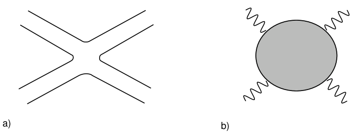
Figure 12: a) The four-point open string tree amplitude. b) Its conformal transform to a disk with four points marked on the boundary.

We will briefly describe here the topological expansion for the case of open strings. A tree-level four-point diagram in this case is shown in Fig. 12a. By a conformal transformation it can be mapped to a disk with four points marked on the boundary (Fig. 12b). These are the positions of insertion of the appropriate vertex operators. Thus, the open string vertex operators are inserted at the boundary of the surface. Open strings can also emit closed strings. In such amplitudes, closed string emission is represented by the insertion of closed string vertex operators in the interior of the surface.

Here the topological expansion also includes Riemann surfaces with boundary. Moreover, we can consider orientable strings (where the string is oriented) as well as non-orientable strings (where the orientation of the string is immaterial). In the second case we will have to include non-orientable Riemann surfaces in the topological expansion. Such a surface is characterized by the number of handles $g$ the number of boundaries $B$, and the number of cross-caps $C$ that introduce the non-orientability of the surface. A cross-cap is a boundary that instead of being $S^{1}$, is $S^{1}/Z_{2}=RP^{1}$. The Euler number is given by

$$\chi=2(1-g)-B-C\,.$$ (8.7)

In Fig. 13 we show the four simplest surfaces with boundaries: the disk with $\chi=1$, the annulus with $\chi=0$, as well as two non-orientable surfaces, the Möbius strip with $\chi=0$ and the Klein bottle with $\chi=0$.

As we will see later on, consistent theories of open unoriented strings necessarily include couplings to closed unoriented strings. An easy way to see this is to consider the annulus diagram (Fig. 13b). If we take time to run upwards, then it describes a one-loop diagram of an open string. If, however, we take time to run sideways then it describes the tree-level propagation of a closed string.

Figure 13: a) The disk. b) The annulus. c) The Möbius strip. d) the Klein bottle.

9 Strings in background fields and low-energy effective actions

So far, we have described the propagation of strings in flat 26-dimensional Minkowski space. We would like, however, to be able to describe string physics when the massless fields $G_{\mu\nu}$, $B_{\mu\nu}$ and $\Phi$ have non-trivial VEVs. This can be done by a finite perturbation of the flat CFT, using the vertex operators for the massless fields. The correct prescription for coupling the dilaton was given by Fradkin and Tseytlin. The Polyakov action becomes

$$S_{P}={1\over 4\pi\alpha^{\prime}}\int d^{2}\xi\left[\sqrt{g}g^{ab}G_{\mu\nu}(X)+\epsilon^{ab}B_{\mu\nu}(X)\right]\partial_{a}X^{\mu}\partial_{b}X_{\nu}+$$

$$+{1\over 8\pi}\int d^{2}\xi\sqrt{g}R^{(2)}\Phi(X)\,,$$ (9.1)

where $R^{(2)}$ is the scalar curvature of the intrinsic word-sheet metric $g_{ab}$. An interesting observation is the following: consider the constant part of the dilaton field (VEV) $\Phi_{0}$. Since the Euler character of the world-sheet is given by

$$\chi={1\over 4\pi}\int\sqrt{g}~{}R^{(2)}\,,$$ (9.2)

we observe that we have a factor $e^{-\chi\Phi_{0}/2}$ in front of $e^{-S_{P}}$. Thus, the string coupling is essentially given by the dilaton VEV

$$g_{\rm string}=e^{\Phi_{0}/2}\,.$$ (9.3)

For general backgrounds, this $\sigma$-model is not conformally invariant. Rather

$${{T_{a}}^{a}\over\sqrt{g}}={\beta^{\Phi}\over 96\pi^{3}}R^{(2)}+{1\over 2\pi}(\beta_{\mu\nu}^{G}{}~{}g^{ab}+\beta_{\mu\nu}^{B}\epsilon^{ab})\partial_{a}X^{\mu}\partial_{b}X_{\nu}\,,$$ (9.4)

where the $\beta$-functions can be obtained perturbatively in the weak coupling expansion of the $\sigma$-model, $\alpha^{\prime}\to 0$. To leading non-trivial order,

$${\beta_{\mu\nu}^{G}\over\alpha^{\prime}}=R_{\mu\nu}-{1\over 4}H_{\mu\rho\sigma}{H_{\nu}}^{\rho\sigma}+\nabla_{\mu}\nabla_{\nu}\Phi+{\cal O}(\alpha^{\prime})\,,$$ (9.5)

$${\beta_{\mu\nu}^{B}\over\alpha^{\prime}}=\nabla^{\mu}\left[e^{-\Phi}~{}H_{\mu\nu\rho}\right]+{\cal O}(\alpha^{\prime})$$ (9.6)

and

$$\beta^{\Phi}=D-26+3\alpha^{\prime}\left[(\nabla\Phi)^{2}-2\hbox{{$\sqcup$}\hbox to0.0pt{\hss$\sqcap$}}\Phi-R+{1\over 12}H^{2}\right]+{\cal O}(\alpha^{\prime 2})\,,$$ (9.7)

where $H_{\mu\nu\rho}$ is the totally antisymmetric field strength of $B_{\mu\nu}$,

$$H_{\mu\nu\rho}=\partial_{\mu}B_{\nu\rho}+\partial_{\nu}B_{\rho\mu}+\partial_{\rho}B_{\mu\nu}$$ (9.8)

and $D$ is the spacetime dimension.

When $G,B,\Phi$ are such that $\beta^{G}_{\mu\nu}=\beta^{B}_{\mu\nu}=0$, then the $\sigma$-model describes a CFT with central charge $c=\beta^{\Phi}$. It can be shown in particular that $\beta^{\Phi}$ is a constant when the other $\beta$-functions vanish.

The conditions for conformal invariance and thus consistent string propagation are given by the equations

$$\beta^{\Phi}=\beta^{G}_{\mu\nu}=\beta^{B}_{\mu\nu}=0\,.$$ (9.9)

These conditions are second-order equations for the background fields and can be obtained from an action

$$\alpha^{\prime D-2}S^{tree}\sim\int d^{D}x\sqrt{-{\rm det}~{}G}e^{-\Phi}\left[R+(\nabla\Phi)^{2}-{1\over 12}H^{2}+{D-26\over 3}\right]+{\cal O}(\alpha^{\prime})\,.$$ (9.10)

At this point it is useful to pause and ask the question: Why do we need conformal invariance? After all, since we are integrating over two-dimensional metrics we expect conformal invariance to be enforced by the integration. In fact we will consider two distinct cases:

$\bullet$ The background fields and spacetime dimension are such that all $\beta$-functions vanish. Then we have conformal invariance at the quantum level, the conformal factor decouples, and we have to factor out its volume from the definition of the path integral. This is the case we considered so far. Moreover, the vanishing of the $\beta$-functions implies, to leading order in $\alpha^{\prime}$, second-order equations for the background fields.

$\bullet$ The $\beta$-functions are not zero. Then the conformal factor does not decouple. Since ${T_{a}}^{a}\sim\delta_{\phi}\log Z$, where $\phi$ is the conformal factor, we can solve this equation to derive the dependence of the effective action on $\phi$. Apart from the Liouville action discussed in (6.7.13), we will also have couplings of $\phi$ to the scalars $X^{\mu}$ if $\beta^{B,G}$ do not vanish. Effectively we have a new $\sigma$-model in $D+1$ dimensions ($\phi$ provides the extra coordinate), which is by construction Weyl-invariant. Thus, we are back to the first case.

We will now consider the notion of the effective action for the light fields. We have seen that (ignoring the tachyon for the moment) the massless fields are $G,B,\Phi$. All other particles have masses of the order of the string scale. We can imagine integrating out the heavy fields that will induce corrections to the action of the light fields. This is the definition of the low-energy effective action. This effective action contains only the light fields and is valid up to energies of the order of the mass of the heavy fields. At tree level, this procedure can be implemented by considering the full (on-shell) scattering amplitudes of the light fields from string calculations, expanding them in $\alpha^{\prime}$ and finding the extra interactions induced on the light fields. A comprehensive exposition of this procedure can be found in [33]. Since the amplitudes used are on-shell, the effective action can be calculated up to terms that vanish by using the equations of motion.

It can be shown that, up to terms that vanish on-shell, the $\sigma$-model conformal invariance conditions and the string amplitude calculations produce the same low-energy effective action (9.10).

In (9.10) the fields that appear are those that couple to the string $\sigma$-model. This is known as the “string frame”. In this frame, the kinetic terms of the metric $G$ and the dilaton are not diagonal. They become diagonal in the “Einstein frame”, related to the string frame by a conformal rescaling of the metric. Separating the expectation value of the dilaton $\Phi\to\Phi_{0}+\Phi$ and defining the Einstein metric as

$$G^{E}_{\mu\nu}=e^{-{2\Phi\over D-2}}G_{\mu\nu}\,,$$ (9.11)

we obtain the action in the Einstein frame:

$$S_{E}^{\rm tree}\sim{1\over\kappa^{2}}\int d^{D}x\sqrt{G^{E}}\left[R-{1\over D-2}(\nabla\Phi)^{2}-{e^{-4\Phi/(D-2)}\over 12}H^{2}\right.$$

$$\left.+e^{2\Phi/(D-2)}{D-26\over 3}\right]+{\cal O}(\alpha^{\prime})\,,$$ (9.12)

where the gravitational constant is given by

$$\kappa=g_{\rm string}\alpha^{\prime(D-2)/2}\,.$$ (9.13)

10 Superstrings and supersymmetry

We have seen so far that bosonic strings suffer from two major problems:

$\bullet$ Their spectrum always contains a tachyon. In that respect their vacuum is unstable.

$\bullet$ They do not contain spacetime fermions.

On the other hand, we have already seen, during our study of free fermion CFTs that they contain states that transform as spinors under the associated orthogonal symmetry. Therefore we should be willing to add free fermions on the world-sheet of the string in order to obtain states that transform as spinors. These fermions should carry a spacetime index, i.e. $\psi^{\mu}$, $\bar{\psi}^{\mu}$, in order for the spinor to be a spacetime spinor. However, in such a case there will be additional negative norm states associated with the modes of $\psi^{0}$. In order for these to be removed from the physical spectrum, we need more constraints than the Virasoro constraints alone. The appropriate result comes from considering an N=1 superconformal algebra of constraints. In the bosonic case, we started with two-dimensional gravity coupled to $D$ scalars $X^{\mu}$ on the world-sheet, which eventually boiled down to a set of Virasoro constraints on the Hilbert space. Here, we would like to start from the two-dimensional N=1 supergravity coupled to $D$ N=1 superfields, each containing a bosonic coordinate $X^{\mu}$ and two fermionic coordinates, one left-moving $\psi^{\mu}$ and one right-moving $\bar{\psi}^{\mu}$. The two-dimensional N=1 supergravity multiplet contains the metric and a gravitino $\chi_{a}$.

The analog of the bosonic Polyakov action is

$$S^{II}_{P}={1\over 4\pi\alpha^{\prime}}\int\sqrt{g}\left[g^{ab}\partial_{a}X^{\mu}\partial_{b}X^{\mu}+{i\over 2}\psi^{\mu}{\partial/}\psi^{\mu}+\quad\quad\quad\quad\right.$$

$$\left.{i\over 2}(\chi_{a}\gamma^{b}\gamma^{a}\psi^{\mu})\left(\partial_{b}X^{\mu}-{i\over 4}\chi_{b}\psi^{\mu}\right)\right]\,.$$ (10.1)

It is invariant under local N=1 left-moving (1,0) supersymmetry

$$\delta g_{ab}=i\epsilon(\gamma_{a}\chi_{b}+\gamma_{b}\chi_{a})\;\;\;,\;\;\;\delta\chi_{a}=2\nabla_{a}\epsilon\,,$$ (10.2)

$$\delta X^{\mu}=i\epsilon\psi^{\mu}\;\;\;,\;\;\;\delta\psi^{\mu}=\gamma^{a}\left(\partial_{a}X^{\mu}-{i\over 2}\chi_{a}\psi^{\mu}\right)\epsilon\;\;\;,\;\;\;\delta\bar{\psi}^{\mu}=0\,,$$ (10.3)

where $\epsilon$ is a left-moving Majorana-Weyl spinor. There is a similar right-moving (0,1) supersymmetry involving a right-moving Majorana-Weyl spinor $\bar{\epsilon}$ and the fermions $\bar{\psi}^{\mu}$. In our notation we have (1,1) supersymmetry.

The analog of the conformal gauge is the superconformal gauge

$$g_{ab}=e^{\phi}\delta_{ab}\;\;\;,\;\;\;\chi_{a}=\gamma_{a}\zeta\,,$$ (10.4)

where $\zeta$ is a constant Majorana spinor; $\phi$ and $\zeta$ decouple from the classical action (10.1). Apart from the Virasoro operators we also have the supercurrents

$$G_{\rm matter}=i\psi^{\mu}\partial X^{\mu}\;\;\;,\;\;\;\bar{G}_{\rm matter}=i\bar{\psi}^{\mu}\bar{\partial}X^{\mu}\,.$$ (10.5)

We also have to introduce the appropriate ghosts. We will still have the usual $b,c$ system with $\lambda=2$ associated with diffeomorphisms, but now we also need a commuting set of ghosts $\beta,\gamma$ with $\epsilon=-1$, $\lambda={\textstyle{3\over 2}}$ associated with the supersymmetry. Superconformal invariance will be present at the quantum level, provided the ghost central charge cancels the matter central charge. Each bosonic and fermionic coordinate contributes $3/2$ to the central charge. Since we have $D$ of them, the matter central charge is $c_{\rm matter}={\textstyle{3\over 2}}D$. The $b,c$ system contributes $-26$ to the central charge while the $\beta,\gamma$ system contributes $+11$. The total central charge vanishes, provided that $D=10$.

The classical constraints imply the vanishing of $T,G,\bar{T},\bar{G}$. Consequently, we have enough constraints to remove the negative norm states.

The BRST current is [26]

$$j_{BRST}=\gamma G_{\rm matter}+cT_{\rm matter}+{1\over 2}\left(cT_{\rm ghost}+\gamma G_{\rm ghost}\right)\,,$$ (10.6)

where

$$G_{\rm matter}=i\psi^{\mu}\partial X^{\mu}\;\;\;,\;\;\;T_{\rm matter}=-{1\over 2}\partial X^{\mu}\partial X^{\mu}-{1\over 2}\psi^{\mu}\partial\psi^{\mu}\,,$$ (10.7)

$$G_{\rm ghost}=-i(c~{}\partial\beta-{1\over 2}\gamma~{}b+{3\over 2}\partial c{}~{}\beta)\;\;\;,\;\;\;T_{\rm ghost}=T_{bc}-{1\over 2}\gamma~{}\partial\beta-{3\over 2}\partial\gamma~{}\beta\,.$$ (10.8)

Exercise. Verify that $G_{\rm ghost}$ and $T_{\rm ghost}$ satisfy the OPEs of the N=1 superconformal algebra (6.5.1),(6.12.7) with the correct central charge.

The BRST charge is

$$Q={1\over 2\pi i}\left[\oint dz~{}j_{BRST}+\oint d\bar{z}~{}\bar{j}_{BRST}\right]\,.$$ (10.9)

It is nilpotent for $D=10$ and can be used in the standard way to define physical states.

10.1 Closed (type-II) superstrings

We will consider first the closed (type-II) superstring case. We will work in a physical gauge and derive the spectrum. The analogue of the light-cone gauge in the supersymmetric case is:

$$X^{+}=x^{+}+p^{+}\tau\;\;\;,\;\;\;\psi^{+}=\bar{\psi}^{+}=0\,.$$ (10.1.1)

As in the bosonic case, we can explicitly solve the constraints by expressing $X^{-},\psi^{-},\bar{\psi}^{-}$ in terms of the transverse modes. Then, the physical states can be constructed out of the transverse bosonic and fermionic oscillators. However, all zero modes are present.

As we mentioned before, we have two left-moving sectors corresponding to $NS$ and $R$ boundary conditions for $\psi^{\mu}$ and $G$ and another two sectors corresponding to $\overline{NS}$ and $\bar{R}$ boundary conditions for $\bar{\psi}^{\mu}$ and $\bar{G}$.

For the moment we will discuss only the left sector to avoid repetition. We will introduce as usual the modes $L_{n}$ and $G_{r}$ of the superconformal generators.

In the light-cone gauge we have solved the constraints, apart from those associated with the zero modes. In the $NS$ sector, $G$ is half-integrally modded and the only zero mode is $L_{0}$. There is also a normal-ordering constant, which can be calculated either by demanding Lorentz invariance of the physical spectrum, as we have done for the bosonic string, or by realizing that in the covariant formulation the lowest “energy” state is not the usual vacuum $|0\rangle$ but $c_{1}\gamma_{-1/2}|0\rangle$. Both approaches result in a normal-ordering constant equal to $a={\textstyle{1\over 2}}$, and $L_{0}-{\textstyle{1\over 2}}$ should be zero on physical states. The state $|p\rangle$ is a physical state with $p^{2}=-m^{2}=2/\alpha^{\prime}$, and it is a tachyon. The next states are of the form $\psi^{i}_{-1/2}|p\rangle$ and satisfy $L_{0}={\textstyle{1\over 2}}$ if $p^{2}=0$. These states are massless. However, we would prefer not to have a tachyonic state. Since the tachyon has $(-1)^{F_{L}}=1$ we would like to impose the extra constraint (GSO projection): physical states in the $NS$ sector should have odd fermion number.

In the $R$ sector we have two zero modes: $L_{0}$ and $G_{0}$. The $L_{0}$ constraint is the same as in the $NS$ sector. A quick look at the expression for $G_{0}$ in (10.5) is enough to convince us that there can be no normal-ordering constant, and that $G_{0}$ should be zero on physical states. On the other hand we know from the superconformal algebra

$$0=\{G_{0},G_{0}\}=2\left(L_{0}-{D-2\over 16}\right)\,.$$ (10.1.2)

Compatibility with the $L_{0}$ constraint implies again that $D=10$. The $R$ ground-states are spinors of O(10). Consequently, these states satisfy the $L_{0}$ constraint. Also remember that $G_{0}=\psi^{\mu}_{0}a_{0}^{\mu}+2\sum_{n\not=0}^{\infty}\psi^{i}_{n}a^{i}_{-n}$. As shown in section 6.11, the operator $\psi^{\mu}_{0}$ is represented by $\gamma^{\mu}$ and $a_{0}^{\mu}$ by $p_{\mu}$. The other terms in $G_{0}$ do not contribute to the ground-states. $G_{0}=0$ implies the Dirac equation $p\!\!\!/\equiv\gamma^{\mu}~{}p_{\mu}=0$. Thus, the potentially massless states in the $R$ sector are a spinor $S$ and a conjugate spinor $C$ of O(10) satisfying the massless Dirac equation. Under $(-1)^{F_{L}}$, $S$ has eigenvalue 1 and $C$ has $-1$. All other states are built on these ground-states and are massive. So far, there is no a priori reason to impose also a GSO projection in the $R$ sector. As we will see later on, one-loop modular invariance will force us to do so. Anticipating this fact, we will also fix the fermion parity in the $R$ sector. Since $(-1)^{F}=$ $plus$ or $minus$ is a matter of convention in the $R$ sector, we will allow both possibilities. We will only keep the $S$ or $C$ spinor ground-states, but not both.

A similar discussion applies to the right-moving sector. Combining the two we have overall four sectors:

$\bullet$ ($NS$-$\overline{NS}$): These are bosons since they transform in tensor representations of the rotation group. The projection here is $(-1)^{F_{L}}=(-1)^{F_{R}}=-1$. The lowest states allowed by the constraint and the GSO projection are of the form $\psi^{i}_{-1/2}\bar{\psi}^{j}_{-1/2}|p\rangle$, they are massless and correspond to a symmetric traceless tensor (the graviton), an antisymmetric tensor and a scalar. The tachyon is gone!

$\bullet$ ($NS$-$\overline{R}$): These are fermions. The GSO projection here is $(-1)^{F_{L}}=-1$ and by convention we keep the $S$ representation in the $\bar{R}$ sector. The lowest-lying states, $\psi^{i}_{-1/2}|p,\bar{S}\rangle$ are massless spacetime fermions and contain a $C$ Majorana-Weyl gravitino and an $S$ fermion.

$\bullet$ ($R$-$\overline{NS}$): Here the GSO projection in $\overline{NS}$ is $(-1)^{F_{R}}=-1$, but in the $R$ sector we have two physically distinct options: keep the S spinor (type-IIB) or the $C$ spinor (type-IIA). Again the lowest-lying states $\bar{\psi}^{i}_{-1/2}|p,S~{}{\rm or}~{}C\rangle$ are massless spacetime fermions.

$\bullet$ ($R$-$\bar{R}$): In the IIA case the massless states are $|S,\bar{C}\rangle$, which decomposes into a vector and a three-index antisymmetric tensor, as will be shown below. In type-IIB they are $|S,\bar{S}\rangle$, which decomposes into a scalar, a two-index antisymmetric tensor, and a self-dual four-index antisymmetric tensor.

There are also the bosonic oscillators for us to use but, as we have seen, they are not involved in the massless states. They do, however, contribute to the massive spectrum.

Both type-IIA and IIB theories have two gravitini and are thus expected to have N=2 local supersymmetry in ten dimensions. In type-IIB the gravitini have the same spacetime chirality, while the two spin ${\textstyle{1\over 2}}$ fermions have opposite chirality. Thus, the theory is chiral. The type-IIA theory is non-chiral since the gravitini and ${\textstyle{1\over 2}}$ fermions have opposite chiralities.

In the light-cone gauge, the left-over constraints are essentially the linearized equations of motion. In the $NS$-$\overline{NS}$ sector the constraints are

$$L_{0}=\bar{L}_{0}\;\;\;,\;\;\;L_{0}-{1\over 2}=0\;;$$ (10.1.3)

and, as we have seen already in the bosonic case, it gives the mass-shell condition. This corresponds to the free Klein-Gordon equation. The $R$-$\overline{NS}$ sector contains spacetime fermions and the constraints are as in (10.1.3), plus the $G_{0}=0$ constraint, which provides as we showed above, the Dirac equation both for massless and massive states. Its square, from (10.1.2), gives the Klein-Gordon equation; the independent equations are thus $G_{0}=0$ and $L_{0}=\bar{L}_{0}$. Similar remarks apply for the $NS$-$\overline{R}$ sector. Finally in the $R$-$\overline{R}$ sector the states are bispinors and they satisfy two Dirac equations: $G_{0}=\bar{G}_{0}=0$. Ramond-Ramond massless states are special for two reasons. First, they are always forms and always coupled to other states via derivatives. No perturbative states are charged under them. As we will see later on, they are in the heart of non-perturbative duality conjectures. A more detailed discussion of their properties can be found in the next section.

We will examine more closely the spacetime meaning of the operators $(-1)^{F_{L,R}}$. In the $NS$ sector

$$(-1)^{F}=\exp\left[i\pi\sum_{r\in Z+1/2}\psi^{i}_{r}\psi^{i}_{-r}\right]\,.$$ (10.1.4)

In the $R$ sector

$$(-1)^{F}=\prod_{\mu=0}^{9}\psi^{\mu}_{0}~{}\exp\left[i\pi\sum_{n=1}^{\infty}\psi^{i}_{n}\psi^{i}_{-n}\right]=\Gamma^{11}~{}\exp\left[i\pi\sum_{n=1}^{\infty}\psi^{i}_{n}\psi^{i}_{-n}\right]\,,$$ (10.1.5)

where $\Gamma^{11}$ is the analog of $\gamma^{5}$ in ten dimensions. We can deduce from the form of the supercurrents (10.5) that the zero modes satisfy

$$\{(-1)^{F_{L}},G_{0}\}=0\;\;\;,\;\;\;\{(-1)^{F_{R}},\bar{G}_{0}\}=0\,.$$ (10.1.6)

These generalize the field theoretic relation

$$\{\Gamma^{11},{\partial/}\}=0\,.$$ (10.1.7)

Note that in string theory this equation holds also for the massive Dirac operator $G_{0}$.

Exercise. Show that at the massless level there is an equal number of on-shell fermionic and bosonic degrees of freedom. This would be necessary if the theory has (at least one) spacetime supersymmetry. Find also the physical states at the next (massive) level both in type-IIA and type-IIB theory. Show that they combine into SO(9) representations, as they should, and that there is again an equal number of fermionic and bosonic degrees of freedom.

We will now study the one-loop vacuum amplitude (or partition function). For the bosonic part of the action we have eight transverse oscillators and, in analogy with the case of the bosonic string, we will get a contribution of $(\sqrt{\tau_{2}}\eta\bar{\eta})^{-8}$. Here, however, we also have the contribution of the world-sheet fermions. We will consider first the IIB case. In the $NS$-$\overline{NS}$ sector the two GSO projections imply that we have the vector on both sides. So the contribution to the partition function is $\chi_{V}\bar{\chi}_{V}$. From the $R$-$\overline{R}$ sector we have projected out the $C$ representation so the contribution is $\chi_{S}\bar{\chi}_{S}$. In the $R$-$\overline{NS}$ and $NS$-$\overline{R}$ sectors we obtain $-\chi_{S}\bar{\chi}_{V}$ and $-\chi_{V}\bar{\chi}_{S}$ respectively. The minus sign is there since spacetime fermions contribute with a minus sign relative to spacetime bosons. So

$$Z^{IIB}={(\chi_{V}-\chi_{S})(\bar{\chi}_{V}-\bar{\chi}_{S})\over(\sqrt{\tau_{2}}\eta~{}\bar{\eta})^{8}}\,.$$ (10.1.8)

Using the formulae (6.11.26) and (6.11.42) for the SO(8) characters, we can write the partition function as

$$Z^{IIB}={1\over(\sqrt{\tau_{2}}\eta\bar{\eta})^{8}}~{}{1\over 2}\sum_{a,b=0}^{1}~{}(-1)^{a+b+ab}~{}{1\over 2}\sum_{\bar{a},\bar{b}=0}^{1}~{}(-1)^{\bar{a}+\bar{b}+\bar{a}\bar{b}}~{}{\vartheta^{4}[^{a}_{b}]~{}\bar{\vartheta}^{4}[^{\bar{a}}_{\bar{b}}]\over\eta^{4}~{}\bar{\eta}^{4}}\,,$$ (10.1.9)

$a=0$ labels the $NS$ sector, $a=1$ the $R$ sector and similarly for the right-movers.

In the type-IIA case, the only difference is that $\chi_{S}$ should be substituted by $\chi_{C}$. The partition function becomes

$$Z^{IIA}={1\over(\sqrt{\tau_{2}}\eta\bar{\eta})^{8}}~{}{1\over 2}\sum_{a,b=0}^{1}~{}(-1)^{a+b}~{}{1\over 2}\sum_{\bar{a},\bar{b}=0}^{1}~{}(-1)^{\bar{a}+\bar{b}+\bar{a}\bar{b}}~{}{\vartheta^{4}[^{a}_{b}]~{}\bar{\vartheta}^{4}[^{\bar{a}}_{\bar{b}}]\over\eta^{4}~{}\bar{\eta}^{4}}\,.$$ (10.1.10)

Exercise. Show that $Z^{IIB},Z^{IIA}$ are modular-invariant. Using (A.18), show that they also are identically zero. This implies that there is at each mass level an equal number of bosonic and fermionic degrees of freedom, consistent with the presence of spacetime supersymmetry.

10.2 Massless $R$-$R$ states

We will now consider in more detail the massless $R$-$R$ states of type-IIA,B string theory, since they have unusual properties and play a central role in non-perturbative duality symmetries. Further reading is to be found in [30].

I will first start by describing in detail the $\Gamma$-matrix conventions in flat ten-dimensional Minkowski space [5].

The ($32\times 32$)-dimensional $\Gamma$-matrices satisfy

$$\{\Gamma^{\mu},\Gamma^{\nu}\}=-2\eta^{\mu\nu}\;\;\;,\;\;\;\eta^{\mu\nu}=(-++\ldots+)\,.$$ (10.2.1)

The $\Gamma$-matrix indices are raised and lowered with the flat Minkowski metric $\eta^{\mu\nu}$:

$$\Gamma_{\mu}=\eta_{\mu\nu}\Gamma^{\nu}\;\;\;\,\;\;\;\Gamma^{\mu}=\eta^{\mu\nu}\Gamma_{\nu}\;.$$ (10.2.2)

We will be in the Majorana representation where the $\Gamma$-matrices are purely imaginary, $\Gamma^{0}$ is antisymmetric, the rest symmetric. Also

$$\Gamma^{0}\Gamma_{\mu}^{\dagger}\Gamma^{0}=\Gamma_{\mu}\;\;\;,\;\;\;\Gamma^{0}\Gamma_{\mu}\Gamma^{0}=-\Gamma_{\mu}^{T}\,.$$ (10.2.3)

Majorana spinors $S_{\alpha}$ are real: $S^{*}_{\alpha}=S_{\alpha}$;

$$\Gamma_{11}=\Gamma_{0}\ldots\Gamma_{9}\;\;\;,\;\;\;(\Gamma_{11})^{2}=1\;\;\;,\;\;\;\{\Gamma_{11},\Gamma^{\mu}\}=0\;;\,.$$ (10.2.4)

$\Gamma_{11}$ is symmetric and real. This is the reason why, in ten dimensions, the Weyl condition $\Gamma_{11}S=\pm S$ is compatible with the Majorana condition. We use the convention that for the Levi-Civita tensor, $\epsilon^{01\ldots 9}=1$. We will define the antisymmetrized products of $\Gamma$-matrices

$$\Gamma^{\mu_{1}\ldots\mu_{k}}={1\over k!}\Gamma^{[\mu_{1}}\ldots\Gamma^{\mu_{k}]}={1\over k!}\left(\Gamma^{\mu_{1}}\ldots\Gamma^{\mu_{k}}\pm{\rm permutations}\right)\,.$$ (10.2.5)

We can derive by straightforward computation the following identities among $\Gamma$-matri-
ces:

$$\Gamma_{11}\Gamma^{\mu_{1}...\mu_{k}} = {(-1)^{[{k\over 2}]}\over(10-k)!}\epsilon^{\mu_{1}...\mu_{10}}\Gamma_{\mu_{k+1}...\mu_{10}}\;,$$ (10.2.6)

$$\Gamma^{\mu_{1}...\mu_{k}}\Gamma_{11} = {(-1)^{[{k+1\over 2}]}\over(10-k)!}\epsilon^{\mu_{1}...\mu_{10}}\Gamma_{\mu_{k+1}...\mu_{10}}\,,$$ (10.2.7)

with $[x]$ denoting the integer part of $x$. Then

$$\Gamma^{\mu}\Gamma^{\nu_{1}...\nu_{k}}=\Gamma^{\mu\nu_{1}...\nu_{k}}-{1\over(k-1)!}\eta^{\mu[\nu_{1}}\Gamma^{\nu_{2}...\nu_{k}]}\,,$$ (10.2.8)

$$\Gamma^{\nu_{1}...\nu_{k}}\Gamma^{\mu}=\Gamma^{\nu_{1}...\nu_{k}\mu}-{1\over(k-1)!}\eta^{\mu[\nu_{k}}\Gamma^{\nu_{1}...\nu_{k-1}]}\,,$$ (10.2.9)

with square brackets denoting the alternating sum over all permutations of the enclosed indices. The invariant Lorentz scalar product of two spinors $\chi,\phi$ is $\chi^{*}_{\alpha}(\Gamma^{0})_{\alpha\beta}\phi_{\beta}$.

Now consider the ground-states of the $R$-$R$ sector. On the left, we have a Majorana spinor $S_{\alpha}$ satisfying $\Gamma_{11}S=S$ by convention. On the right, we have another Majorana spinor $\tilde{S}_{\alpha}$ satisfying $\Gamma_{11}\tilde{S}=\xi\tilde{S}$, where $\xi=1$ for the type-IIB string and $\xi=-1$ for the type-IIA string. The total ground-state is the product of the two. To represent it, it is convenient to define the following bispinor field

$$F_{\alpha\beta}=S_{\alpha}(i\Gamma^{0})_{\beta\gamma}\tilde{S}_{\gamma}\,.$$ (10.2.10)

With this definition, $F_{\alpha\beta}$ is real and the trace $F_{\alpha\beta}\delta^{\alpha\beta}$ is Lorentz-invariant. The chirality conditions on the spinor translate into

$$\Gamma_{11}F=F\;\;\;,\;\;\;F\Gamma_{11}=-\xi F\,,$$ (10.2.11)

where we have used the fact that $\Gamma_{11}$ is symmetric and anticommutes with $\Gamma^{0}$.

We can now expand the bispinor $F$ into the complete set of antisymmetrized $\Gamma$’s:

$$F_{\alpha\beta}=\sum_{k=0}^{10}{i^{k}\over k!}F_{\mu_{1}\ldots\mu_{k}}(\Gamma^{\mu_{1}\ldots\mu_{k}})_{\alpha\beta}\,,$$ (10.2.12)

where the $k=0$ term is proportional to the unit matrix and the tensors $F_{\mu_{1}\ldots\mu_{k}}$ are real.

We can now translate the first of the chirality conditions in (10.2.11) using (10.2.7) to obtain the following equation:

$$F^{\mu_{1}\ldots\mu_{k}}={(-1)^{\left[{k+1\over 2}\right]}\over(10-k)!}\epsilon^{\mu_{1}\ldots\mu_{10}}F_{\mu_{k+1}\ldots\mu_{10}}\,.$$ (10.2.13)

The second chirality condition implies

$$F^{\mu_{1}\ldots\mu_{k}}=\xi{(-1)^{\left[{k\over 2}\right]+1}\over(10-k)!}\epsilon^{\mu_{1}\ldots\mu_{10}}F_{\mu_{k+1}\ldots\mu_{10}}\,.$$ (10.2.14)

Compatibility between (10.2.13) and (10.2.14) implies that type-IIB theory ($\xi=1$) contains tensors of odd rank (the independent ones being k=1,3 and k=5 satisfying a selfduality condition) and type-IIA theory ($\xi=-1)$ contains tensors of even rank (the independent ones having k=0,2,4). The number of independent tensor components adds up in both cases to $16\times 16=256$.

As mentioned in section 10.1, the mass-shell conditions imply that the bispinor field ( 10.2.1) obeys two massless Dirac equations coming from $G_{0}$ and $\bar{G}_{0}$:

$$(p_{\mu}\Gamma^{\mu})F=F(p_{\mu}\Gamma^{\mu})=0\ \,.$$ (10.2.15)

To convert these to equations for the tensors, we use the gamma identities (10.2.8) and (10.2.9). After some straightforward algebra one finds

$$p^{[\mu}F^{\nu_{1}...\nu_{k}]}=p_{\mu}F^{\mu\nu_{2}...\nu_{k}}=0\,,$$ (10.2.16)

which are the Bianchi identity and the free massless equation for an antisymmetric tensor field strength. We may write these in economic form as

$$dF=d\ ^{*}F=0\,.$$ (10.2.17)

Solving the Bianchi identity locally allows us to express the $k$-index field strength as the exterior derivative of a $(k-1)$-form potential

$$F_{\mu_{1}...\mu_{k}}={1\over(k-1)!}\partial_{[\mu_{1}}C_{\mu_{2}...\mu_{k}]}\,,$$ (10.2.18)

or in short-hand notation

$$F_{(k)}=dC_{(k-1)}\,.$$ (10.2.19)

Consequently, the type-IIA theory has a vector ($C^{\mu}$) and a three-index tensor potential ($C^{\mu\nu\rho}$) , in addition to a constant non-propagating zero-form field strength ($F$), while the type-IIB theory has a zero-form ($C$), a two-form ($C^{\mu\nu}$) and a four-form potential ($C^{\mu\nu\rho\sigma}$), the latter with self-dual field strength. The number of physical transverse degrees of freedom adds up in both cases to $64=8\times 8$.

It is not difficult to see that in the perturbative string spectrum there are no states charged under the $R$-$R$ forms. First, couplings of the form $\langle s|R\overline{R}|s\rangle$ are not allowed by the separately conserved left and right fermion numbers. Second, the $R$-$R$ vertex operators contain the field strengths rather than the potentials and equations of motion and Bianchi identities enter on an equal footing. If there were electric states in perturbation theory we would also have magnetic states.

$R$-$R$ forms have another peculiarity. There are various ways to deduce that their couplings to the dilaton are exotic. The dilaton dependence of an $F^{2m}$ term at the k-th order of perturbation theory is $e^{(k-1)\Phi}e^{m\Phi}$ instead of the usual $e^{(k-1)\Phi}$ term for $NS$-$NS$ fields. For example, at tree-level, the quadratic terms are dilaton-independent.

10.3 Type-I superstrings

We will now consider open superstrings. There are two possibilities: oriented and unoriented open superstrings. Unoriented open strings are obtained by identifying open strings by the operation that exchanges the two end-points. The bosonic case was discussed earlier. We had seen that we can add Chan-Paton factors at the end-points. In the oriented case we obtained a U(N) gauge group, while in the unoriented case we obtained O(N) or Sp(N) gauge groups. As usual, in the superstring case, the GSO projection will remove the tachyonic ground-state and the lowest bosonic states will be a collection of massless vectors.

From the Ramond sector we will obtain a Majorana-Weyl spinor in the adjoint of the gauge group. Thus, the massless spectrum in the open sector would consist of a ten-dimensional Yang-Mills supermultiplet. Anticipating the discussion on anomalies in the next chapter we will point out that Yang-Mills theory in ten dimensions has gravitational and gauge anomalies for any gauge group. It is necessary to couple the open strings with appropriate closed strings for the resulting theory to be anomaly-free. The only anomaly-free possibility turns out to be the unoriented O(32) open string theory.

The modern way to make this construction uses the concept of the orientifold. An orientifold is a generalization of the orbifold concept: along with the projection acting on the target space, there is a projection acting also on the world-sheet. This projection is an orientation-reversal (parity) operation on the world-sheet $\Omega$: $z\leftrightarrow\bar{z}$ or in terms of the cylinder coordinates $\tau,\sigma$: $\sigma\to-\sigma$. For this to be a symmetry we must start with a left-right-symmetric closed superstring theory. From the type-IIA,B theories that we have considered so far only IIB is left-right-symmetric (Ramond ground-states of same chirality on left and right). We will thus consider the IIB string and construct its orientifold using the world-sheet parity operation as the projection operator. As in the case of standard orbifolds, we will have an untwisted sector that contains the invariant states of the original theory. We will first find what the untwisted sector is, in our case.

In the $NS$-$\overline{NS}$ sector, the states that survive are the graviton and a scalar (the dilaton). The antisymmetric tensor, being an antisymmetrized product of left and right oscillators, is projected out. In the $R$-$\overline{R}$ sector the two-index antisymmetric tensor survives, but the scalar and the four-index self-dual antisymmetric tensor are projected out. Finally from the fermionic sectors that contain two Majorana-Weyl gravitini and two Majorana-Weyl fermions we obtain just half of them. Thus, in total, we have the graviton, a scalar and antisymmetric tensor, as well as a Majorana-Weyl gravitino and a Majorana-Weyl fermion. This is the content of the (chiral) N=1 supergravity multiplet in ten dimensions. To summarize, the untwisted sector of the orientifold contains unoriented closed strings.

What is the twisted sector? We usually define it by imposing a periodicity condition together with the orbifold transformation, which we will also do here:

$$X(\sigma+2\pi)=X(2\pi-\sigma)$$ (10.3.1)

and similarly for the fermions. Using also the fact that they satisfy the two-dimensional Laplace equation $\partial^{2}_{\tau}-\partial_{\sigma}^{2}=0$, we can show that the solutions with these boundary conditions can be written as a sum of open string coordinates satisfying Neumann boundary conditions at both end-points and open string coordinates satisfying Dirichlet-Neumann boundary conditions. It turns out that consistency (tadpole cancelation) demands that the second kind of oscillators to be absent. The upshot of all this is that the twisted sector is the open superstring. In this context, we can interpret the Chan-Paton factors as labels of the twisted sector ground-states. Thus, together with the untwisted (closed string) sector, we obtain that the massless sector is ten-dimensional N=1 supergravity coupled to N=1 super-Yang-Mills. This is the (unoriented) type-I superstring theory. As we will see later on, anomaly cancelation restricts the gauge group to be O(32).

10.4 Heterotic superstrings

So far, we have seen that we could use either the Virasoro algebra (bosonic strings) or the N=1 superconformal algebra (superstrings) to remove ghosts from string theories. Moreover, the closed theories were left-right symmetric, in the sense that a similar algebra is acting on both the left and right. We might however envisage the possibility of using a Virasoro algebra on the left and the superconformal algebra on the right.

Consider a string theory where we have on the left side a number of bosonic coordinates and an equal number of left-moving word-sheet fermions. The left constraint algebra will be that of the superstring and, the absence of Weyl anomaly will imply that the number of left-moving coordinates must be 10. In the right-moving sector, we will include just a number of bosonic coordinates. The constraint algebra will be the Virasoro algebra and the Weyl anomaly cancelation implies that the number of right-moving coordinates is 26. Together, we have ten left+right bosonic coordinates $X^{\mu}(z,\bar{z})$, ten left-moving fermions $\psi^{\mu}(z)$ and an extra sixteen right-moving coordinates $\phi^{I}(\bar{z})$, $I=1,2,\dots,16$. The $X^{\mu}$ are non-compact, but the $\phi^{I}$ are necessarily compact (for reasons of modular invariance) and must take values in some sixteen-dimensional lattice $L_{16}$. To remove the tachyon, we will also impose the usual GSO projection on the left, namely $(-1)^{F}=-1$. Here, we will have two sectors, generated by the left-moving fermions, the $NS$ sector (spacetime bosons) and the $R$ sector (spacetime bosons). Also the non-compact spacetime dimension is ten, the $\phi^{I}$ being compact (“internal”) coordinates.

We will try to compute the one-loop partition function in this case (light-cone gauge). The eight transverse non-compact bosons contribute as usual $(\sqrt{\tau_{2}}\eta\bar{\eta})^{-8}$. The left-moving fermions contribute (due to the GSO projection) $\chi_{V}-\chi_{S}$. Finally the contribution of the right-moving compact bosons $\phi^{I}$ can be obtained by taking the right-moving part of the toroidal CFT (7.1.38):

$$Z_{\rm compact}(\bar{q})=\sum_{L_{16}}~{}{\bar{q}^{\vec{p}_{R}^{2}\over 2}\over\bar{\eta}^{16}}={\bar{\Gamma}_{16}(\bar{q})\over\bar{\eta}^{16}}\,,$$ (10.4.1)

where $\vec{p}_{R}$ is a lattice vector. Putting everything together we obtain

$$Z^{\rm heterotic}={1\over(\sqrt{\tau_{2}}\eta\bar{\eta})^{8}}~{}{\bar{\Gamma}_{16}\over\bar{\eta}^{16}}~{}{1\over 2}\sum_{a,b=0}^{1}~{}(-1)^{a+b+ab}{\vartheta[^{a}_{b}]^{4}\over\eta^{4}}\,.$$ (10.4.2)

In order for $Z^{\rm heterotic}$ to be modular-invariant, the lattice sum $\bar{\Gamma}_{16}$ must be invariant under $\tau\to\tau+1$, which implies that the lattice must be even (${\vec{p}_{R}}^{2}=$ even integer). It must also transform as

$$\tau\to-{1\over\tau}\;\;:\;\;\bar{\Gamma}_{16}\to\bar{\tau}^{8}~{}\bar{\Gamma}_{16}\,,$$ (10.4.3)

which implies that the lattice is self-dual (the dual of the lattice coincides with the lattice itself). There are two sixteen-dimensional lattices that satisfy the above requirements:

$\bullet$ $\rm E_{8}\times E_{8}$ lattice. This is the root lattice of the group $\rm E_{8}\times E_{8}$. The roots of E₈ are composed of the roots of O(16), $\vec{\epsilon}_{ij}$, which are eight-dimensional vectors with a $\pm 1$ in position i, a $\pm 1$ in position j and zero elsewhere, as well as the spinor weights of O(16), $\vec{\epsilon}^{s}_{\alpha}=(\zeta_{1},\zeta_{2},\cdots,\zeta_{8})/2$, $\alpha=1,2,\cdots,128$, with $\zeta_{i}=\pm 1$, and $\sum_{i}\zeta_{i}=0~{}{\rm mod}~{}(4)$. The roots have squared length equal to 2. A general lattice vector can be written as $\sum_{i<j}n_{ij}\vec{\epsilon}_{ij}+\sum_{\alpha}m_{\alpha}\vec{\epsilon}^{s}_{\alpha}$, with $n_{ij},m_{\alpha}\in Z$. The lattice sum can be written in terms of $\vartheta$-functions as

$$\bar{\Gamma}_{\rm E_{8}\times E_{8}}=(\bar{\Gamma}_{8})^{2}=\left[{1\over 2}\sum_{a,b=0,1}~{}\bar{\vartheta}[^{a}_{b}]^{8}\right]^{2}=1+2\cdot 240~{}\bar{q}+{\cal O}(\bar{q}^{2})\,.$$ (10.4.4)

Combining it with the oscillators, we observe that there are $2\cdot 240+16=2\cdot 248$ states with $\bar{L}_{0}=1$, which make the adjoint representation of $\rm E_{8}\times E_{8}$. In fact this left-moving theory realizes the current algebra of $\rm E_{8}\times E_{8}$ both at level 1. The only integrable representation is the vacuum representation, and the first non-trivial states above the vacuum are generated by the current modes $\bar{J}_{-1}^{a}$.

$\bullet$ $\rm O(32)/Z_{2}$ lattice. This is the root lattice of O(32) augmented by one of the two spinor weights. The roots of O(32) are $\vec{\epsilon}_{ij}$, which are sixteen-dimensional vectors with a $\pm 1$ in position i, a $\pm 1$ in position j and zero elsewhere. The spinor weights are $\vec{\epsilon}^{s}_{\alpha}=(\zeta_{1},\zeta_{2},\cdots,\zeta_{16})/2$, $\alpha=1,2,3,\cdots,2^{16}$, with $\zeta_{i}=\pm 1$, and $\sum_{i}\zeta_{i}=0~{}{\rm mod}~{}(4)$. The roots have squared length equal to 2. The generic lattice vector is $\sum_{i<j}n_{ij}\vec{\epsilon}_{ij}+\sum_{\alpha}m_{\alpha}\vec{\epsilon}^{s}_{\alpha}$, with $n_{ij},m_{\alpha}\in Z$. The lattice sum can be written as

$$\bar{\Gamma}_{\rm O(32)/Z_{2}}={1\over 2}\sum_{a,b=0,1}~{}\bar{\vartheta}[^{a}_{b}]^{16}=1+480~{}\bar{q}+{\cal O}(\bar{q}^{2})\,.$$ (10.4.5)

This theory has a O(32) right-moving current algebra at level 1. The integrable representations that participate are the vacuum and the spinor and again the states at $\bar{L}_{0}=1$ come from the current modes $\bar{J}^{a}_{-1}$. The spinor ground-states have $\bar{L}_{0}=2$.

Both right-moving current algebra theories can also be constructed from 32 free right-moving fermions $\bar{\psi}^{i}$, $i=1,2,\dots,32$. We will start from the O(32)/Z₂ theory. The currents

$$\bar{J}^{ij}=i\bar{\psi}^{i}\bar{\psi}^{j}$$ (10.4.6)

form the level-one O(32) current algebra. In the Ramond sector, all fermions are periodic, in which case O(32) invariance is not broken and we obtain the two spinors $S,C$ of O(32). Finally imposing a GSO-like projection $(-1)^{F}=1$ keeps the vacuum representation in the $NS$ sector and one of the spinors in the $R$ sector.

For the $\rm E_{8}\times E_{8}$ theory we will consider separate periodic or antiperiodic conditions for the two groups of sixteen fermions. In this case the O(32) invariance is broken to $\rm O(16)\times O(16)$. In the Ramond sector, however, we obtain one of the spinors of O(16) with $\bar{L}_{0}=1$. This spinor combines with the adjoint of O(16) to make the adjoint of $\rm E_{8}$.

We can now describe the massless spectrum of the heterotic string theory (light-cone gauge). In the $NS$ sector the constraints are

$$L_{0}={1\over 2}\;\;\;,\;\;\;\bar{L}_{0}=1\,.$$ (10.4.7)

Taking also into account the GSO projection, we find that there is no tachyon and the massless states are $\psi^{i}_{-1/2}\bar{a}^{j}_{-1}|p\rangle$, which gives the graviton, antisymmetric tensor and dilaton, and $\psi^{i}_{-1/2}\bar{J}^{a}_{-1}|p\rangle$, which gives vectors in the adjoint of $\rm G=E_{8}\times E_{8}$ or O(32).

In the $R$ sector the independent constraints are

$$G_{0}=0\;\;\;,\;\;\;\bar{L}_{0}=1\,,$$ (10.4.8)

which, together with the GSO condition, give a Majorana-Weyl gravitino, a Majorana-Weyl fermion, and a set of Majorana-Weyl fermions in the adjoint of the gauge group G. The theory has N=1 supersymmetry in ten dimensions and contains at the massless level the supergravity multiplet, and a vector supermultiplet in the adjoint of G. Moreover, the theory is chiral.

There is another interesting heterotic theory we can construct in ten dimensions. This can be obtained as a $Z_{2}$ orbifold of the $\rm E_{8}\times E_{8}$ theory. The first symmetry we will use is $(-1)^{F}$. In each of the two $\rm E_{8}$’s there is also a symmetry that leaves the vector of the O(16) subgroup invariant and changes the sign of the O(16) spinor. We will call this symmetry generator ${\cal S}_{i}$, $i=1,2$ acting on the first, respectively second $\rm E_{8}$’s. The $Z_{2}$ element by which we will orbifold is $(-1)^{F+1}~{}{\cal S}_{1}~{}{\cal S}_{2}$. We will construct the orbifold blocks. In the sector of the left-moving world-sheet fermions only $(-1)^{F+1}$ acts non-trivially. Using (6.11.26) and (6.11.42) we can see that $(-1)^{F+1}$ acts as unity on the vector and as $-1$ on the spinor. The twisted blocks are

$$Z_{\rm fermions}[^{h}_{g}]={1\over 2}\sum_{a,b=0}^{1}~{}(-1)^{a+b+ab+ag+bh+gh}~{}{\vartheta^{4}[^{a}_{b}]\over\eta^{4}}\,.$$ (10.4.9)

On each of the $\rm E_{8}$’s the non-trivial projection is ${\cal S}_{i}$, which gives the following orbifold blocks

$$\bar{Z}_{E_{8}}[^{h}_{g}]={1\over 2}\sum_{\gamma,\delta=0}^{1}~{}(-1)^{\gamma g+\delta h}{}~{}{\bar{\vartheta}^{8}[^{\gamma}_{\delta}]\over\bar{\eta}^{8}}\,.$$ (10.4.10)

The total partition function is

$$Z^{\rm heterotic}_{\rm O(16)\times O(16)}={1\over 2}\sum_{h,g=0}^{1}~{}{\bar{Z}_{E_{8}}[^{h}_{g}]^{2}\over(\sqrt{\tau_{2}}\eta\bar{\eta})^{8}}~{}{1\over 2}\sum_{a,b=0}^{1}~{}(-1)^{a+b+ab+ag+bh+gh}~{}{\vartheta^{4}[^{a}_{b}]\over\eta^{4}}\,.$$ (10.4.11)

Exercise. Show that (10.4.11) is modular-invariant. Show also that it describes a ten-dimensional theory with gauge group $\rm O(16)\times O(16)$ and find the massless spectrum. Is this theory supersymmetric ?

Exercise. To construct the partition functions of ten-dimensional heterotic theories we need in general the characters of O(8) for the left-moving fermions and the characters of a rank 16, level one current algebra for the internal right-moving part (the bosonic contribution is always the same). Consider first the case G=O(32). Write the most general partition function as linear combinations of the characters, and then impose the following constraints:

$\bullet$ Normalization of the vacuum contribution to 1.

$\bullet$ Modular invariance.

$\bullet$ Correct spin-statistics relation.

$\bullet$ Absence of tachyons.

How many theories do you find? How many are supersymmetric?

Repeat the procedure above for $\rm G=E_{8}\times O(16)$ and $\rm O(16)\times O(16)$.

10.5 Superstring vertex operators

In analogy with the bosonic string, the vertex operators must be primary states of the superconformal algebra. Using chiral superfield language (see (6.12.12),(6.12.13)) where

$$\hat{X}^{\mu}(z,\theta)=X^{\mu}(z)+\theta\psi^{\mu}(z)\,.$$ (10.5.1)

The left-moving vertex operators can be written in the form:

$$\int dz~{}\int d\theta~{}V(z,\theta)=\int dz~{}\int d\theta{}~{}(V_{0}(z)+\theta V_{-1}(z))=\int dz~{}V_{-1}\,.$$ (10.5.2)

The conformal weight of $V_{0}$ is ${\textstyle{1\over 2}}$ while that of $V_{-1}$ is 1. The integral of $V_{-1}$ has conformal weight zero. For the massless spacetime bosons the vertex operator is

$$V^{\rm boson}(\epsilon,p,z,\theta)=\epsilon_{\mu}:D\hat{X}^{\mu}~{}e^{ip\cdot\hat{X}}\,,$$ (10.5.3)

$$V_{0}^{\rm boson}=\epsilon_{\mu}\psi^{\mu}e^{ip\cdot X}\;\;\;,\;\;\;V^{\rm boson}_{-1}(\epsilon,p,z)=\epsilon_{\mu}:(\partial X^{\mu}+ip\cdot\psi~{}\psi^{\mu})e^{ip\cdot X}:\,,$$ (10.5.4)

where $\epsilon\cdot p=0$. In the covariant picture this vertex operator becomes

$$V^{\rm boson}_{-1}(\epsilon,p,z)=[Q_{\rm BRST},\xi(z)e^{-\phi(z)}\epsilon\cdot\psi~{}e^{ip\cdot X}]\,.$$ (10.5.5)

The spacetime fermion vertex operators can only be constructed in the covariant formalism. For the massless states ($p^{2}=0$) they are of the form

$$V^{\rm fermion}_{-1/2}(u,p,z)=u^{\alpha}(p):e^{-{\phi(z)/2}}~{}S_{\alpha}(z)~{}e^{ip\cdot X}:\,,$$ (10.5.6)

$\phi$ is the boson coming from the bosonization of the $\beta,\gamma$ superconformal ghosts, $e^{-\phi/2}$ is the spin field of the $\beta,\gamma$ system of conformal weight 3/8 (see section 6.15) and $S_{\alpha}$ is the spin field of the fermions $\psi^{\mu}$ forming an O(10)₁ current algebra, with weight 5/8 (see section 6.11). The subscript $-1/2$ indicates the $\phi$-charge. The total conformal weight of $V_{-1/2}$ is 1. Finally, $u^{\alpha}$ is a spinor satisfying the massless Dirac equation $p/u=0$.

There is a subtlety in the case of fermionic strings having to do with the $\beta,\gamma$ system. As we have seen, in the bosonized form, the presence of the background charge alters the charge neutrality condition. This is related to the existence of supermoduli or superkilling spinors. Thus, depending on the correlation function and surface we must have different representatives for the vertex operators of a given physical state with different $\phi$-charges. This can be done in the following way. Consider a physical vertex operator with $\phi$ charge $q$, $V_{q}$. It is BRST invariant, $[Q_{\rm BRST},V_{q}]=0$. We can construct another physical vertex operator representing the same physical state but with charge $q+1$ as $V_{q+1}=[Q_{\rm BRST},\xi V_{q}]$ since $Q_{\rm BRST}$ carries charge 1. Since it is a BRST commutator, $V_{q+1}$ is also BRST-invariant. However, we have seen that states that are BRST commutators of physical states are spurious. In this case this is avoided since the $\xi$ field appears in the commutator and its zero mode lies outside the ghost Hilbert space. The different $\phi$ charges are usually called pictures in the literature. The ${\textstyle{1\over 2}}$ picture for the fermion vertex can be computed to be

$$V_{1/2}^{\rm fermion}(u,p) = [Q_{\rm BRST},\xi(z)V_{-1/2}^{\rm fermion}(u,p,z)]$$ (10.5.7)

$$= u^{\alpha}(p)e^{\phi/2}S_{\alpha}e^{ip\cdot X}+\cdots\,,$$

where the ellipsis involves terms that do not contribute to four-point amplitudes. The ten-dimensional spacetime supersymmetry charges can be constructed from the fermion vertex at zero momentum,

$$Q_{\alpha}={1\over 2\pi i}\oint dz~{}:e^{-{\phi(z)/2}}~{}S_{\alpha}(z)\,.$$ (10.5.8)

It transforms fermions into bosons and vice versa

$$[Q_{\alpha},V^{\rm fermion}_{-1/2}(u,p,z)]=V^{\rm boson}_{-1}(\epsilon^{\mu}=u^{\beta}\gamma^{\mu}_{\beta\alpha},p,z)\,,$$ (10.5.9)

$$[Q_{\alpha},V^{\rm boson}_{0}(\epsilon,p,z)]=V^{\rm fermion}_{-1/2}(u^{\beta}=ip^{\mu}\epsilon^{\nu}(\gamma_{\mu\nu})^{\beta}_{\alpha},p,z)\,.$$ (10.5.10)

There are various pictures for the supersymmetry charges also.

10.6 Supersymmetric effective actions

So far we have seen that, in ten dimensions, there are the following spacetime supersymmetric string theories.

$\bullet$ Type-I theory (chiral) with N=1 supersymmetry and gauge group O(32).

$\bullet$ Heterotic theories (chiral) with N=1 supersymmetry and gauge groups O(32) and E${}_{8}\times$E₈.

$\bullet$ Type-IIA theory (non-chiral) with N=2 supersymmetry.

$\bullet$ Type-IIB theory (chiral) with N=2 supersymmetry.

We would like to find the effective field theories that describe the dynamics of the massless fields. A straightforward approach would be the one we used in the bosonic case, namely either extracting them from scattering amplitudes or requiring Weyl invariance of the associated $\sigma$-model in general background fields. In the presence of supersymmetry, however, these effective actions are uniquely fixed. They have been constructed during the late seventies, early eighties, as supergravity theories.

First we would like to obtain the low-energy effective action at the leading order approximation. When only bosonic fields are present, we just have to keep terms of up to two derivatives. In the presence of fermions, however, we would like to modify our counting rules a bit so that the kinetic terms $\phi\hbox{{$\sqcup$}\hbox to0.0pt{\hss$\sqcap$}}\phi$ for bosons and $\bar{\psi}{\partial/}\psi$ for fermions are equally important at low energy. We will give weight 0 to bosons, weight ${\textstyle{1\over 2}}$ to fermions and 1 to a derivative. Then, both kinetic terms have the same weight, namely 2. These weights are also respected by supersymmetry (SUSY) as can be directly verified from the generic SUSY transformations

$$\delta_{\epsilon}\phi\sim\phi^{m}~{}\psi\epsilon\;\;\;,\;\;\;\delta_{\epsilon}\psi\sim\partial\phi^{m}~{}\epsilon+\phi^{m}~{}\psi^{2}\epsilon\,.$$ (10.6.1)

The effective actions in the leading order must have weight 2, and this is true for all supergravity actions.

In ten dimensions, in order to have massless fields with spin not greater than 2 we have to restrict ourselves to N$\leq 2$ SUSY.

We will first consider N=1 supersymmetry. There are two massless supersymmetry representations (supermultiplets). The vector multiplet contains a vector ($A_{\mu}$) and a Majorana-Weyl fermion ($\chi_{\alpha}$). The supergravity multiplet contains the graviton ($g_{\mu\nu}$), antisymmetric tensor ($B_{\mu\nu}$) and a scalar $\phi$ (dilaton) as well as a Majorana-Weyl gravitino ($\psi^{\mu}_{\alpha}$) and a Majorana-Weyl fermion ($\lambda_{\alpha}$). The effective action of an N=1 supergravity coupled to super Yang-Mills is fixed by supersymmetry, the only choice that remains being that of the gauge group. The super Yang-Mills action is (in the absence of gravity)

$$L_{\rm YM}=-{1\over 4}F^{a}_{\mu\nu}F^{a,\mu\nu}-\bar{\chi}^{a}\Gamma^{\mu}D_{\mu}\chi^{a}\,,$$ (10.6.2)

where

$$F^{a}_{\mu\nu}=\partial_{\mu}A^{a}_{\nu}-\partial_{\nu}A^{a}_{\mu}+g{f^{a}}_{bc}A^{b}_{\mu}A^{c}_{\nu}\,,$$ (10.6.3)

$$D_{\mu}\chi^{a}=\partial_{\mu}\chi^{a}+g{f^{a}}_{bc}A^{b}_{\mu}\chi^{c}$$ (10.6.4)

and $g$ is the Yang-Mills coupling constant. The pure N=1 supergravity action is

$$L_{\rm SUGRA}^{N=1} = -{1\over 2\kappa^{2}}R-{3\over 4}\phi^{-3/2}H_{\mu\nu\rho}H^{\mu\nu\rho}-{9\over 16\kappa^{2}}{\partial_{\mu}\phi\partial^{\mu}\phi\over\phi^{2}}-{1\over 2}\bar{\psi}^{\mu}\Gamma^{\mu\nu\rho}\nabla_{\nu}\psi_{\rho}-$$ (10.6.5)

$$-{1\over 2}\bar{\lambda}\Gamma^{\mu}\nabla_{\mu}\lambda-{3\sqrt{2}\over 8}{\partial_{\nu}\over\phi}\bar{\psi}^{\mu}\Gamma^{\nu}\Gamma^{\mu}\lambda+{\sqrt{2}\kappa\over 16}\phi^{-3/4}H_{\nu\rho\sigma}\left[\bar{\psi}_{\mu}\Gamma^{\mu\nu\rho\sigma\tau}\psi_{\tau}+\right.$$

$$\left.+6\bar{\psi}^{\nu}\Gamma^{\rho}\psi^{\sigma}-\sqrt{2}\bar{\psi}_{\mu}\Gamma^{\nu\rho\sigma}\Gamma^{\mu}\lambda\right]+({\rm Fermi})^{4}\,,$$

where $\kappa$ is Newton’s constant, $\Gamma^{\mu_{1}\dots\mu_{n}}$ stands for the completely antisymmetrized product of $\Gamma$ matrices, $H_{\mu\nu\rho}$ is given in (9.8) and we did not write explicitly terms involving four fermions.

The two actions can be coupled together

$$L^{N=1}_{\rm SUGRA+YM}={L^{N=1}_{\rm SUGRA}}^{\prime}+\phi^{-3/4}~{}L^{\prime}_{\rm YM}\,.$$ (10.6.6)

The prime in the Yang-Mills action implies that covariant derivatives now contain the spin connection. The prime in the supergravity action implies that we have to modify the definition of the field strength of $B$:

$$\hat{H}_{\mu\nu\rho}=H_{\mu\nu\rho}-{\kappa\over\sqrt{2}}\omega^{CS}_{\mu\nu\rho}\,,$$ (10.6.7)

where the Chern-Simons form is

$$\omega^{CS}_{\mu\nu\rho}=A^{a}_{\mu}F^{a}_{\nu\rho}-{g\over 3}f_{abc}A^{a}_{\mu}A^{b}_{\nu}A^{c}_{\rho}+{\rm cyclic}\,.$$ (10.6.8)

This modification implies that in order for the full theory to be gauge-invariant the antisymmetric tensor must transform under gauge transformations $\delta A\to d\Lambda+[A,\Lambda]$ as

$$\delta B={\kappa\over\sqrt{2}}{\rm Tr}[\Lambda dA]\,,$$ (10.6.9)

so that the modified field strength $\hat{H}$ is invariant.

The theory contains a single parameter, since the combination $g^{4}/\kappa^{3}$ is dimensionless and can be scaled to 1 by a rescaling of the field $\phi$.

When we have two supersymmetries, there are only two possibilities:

$\bullet$ $\@@underline{\hbox{Type-IIA supergravity}}$. This is the low energy limit of the type-IIA superstring in ten dimensions. It contains a single supermultiplet of N=2 supersymmetry containing the graviton ($g_{\mu\nu}$), an antisymmetric tensor ($B_{\mu\nu}$), a scalar $\phi$ (dilaton), a vector $A_{\mu}$ and a three-index antisymmetric tensor $C_{\mu\nu\rho}$ as well as a Majorana gravitino ($\psi^{\mu}_{\alpha}$) and a Majorana fermion ($\lambda_{\alpha}$). The supergravity action is completely fixed and can be obtained by dimensional reduction of the eleven-dimensional N=1 supergravity [31] containing the eleven-dimensional metric $G_{\mu\nu}$ and a three-index antisymmetric tensor $\hat{C}_{\mu\nu\rho}$. The action is

$$L^{D=11} = {1\over 2\kappa^{2}}\left[R-{1\over 2\cdot 4!}G_{4}^{2}\right]-i\bar{\psi}_{\mu}\Gamma^{\mu\nu\rho}\tilde{\nabla}_{\nu}\psi_{\rho}+{1\over 2\kappa^{2}(144)^{2}}G_{4}\wedge G_{4}\wedge\hat{C}+$$ (10.6.10)

$$+{1\over 192}\left[\bar{\psi}_{\mu}\Gamma^{\mu\nu\rho\sigma\tau\upsilon}\psi_{\upsilon}+12\bar{\psi}^{\nu}\Gamma^{\rho\sigma}\psi^{\tau}\right](G+\hat{G})_{\nu\rho\sigma\tau}\,,$$

where $\tilde{\nabla}$ is defined with respect to the connection $(\omega+\tilde{\omega})/2$, and $\omega$ is the spin connection while

$$\tilde{\omega}_{\mu,ab}=\omega_{\mu,ab}+{i\kappa^{2}\over 4}\left[-\bar{\psi}^{\nu}\Gamma_{\nu\mu ab\rho}\psi^{\rho}+2(\bar{\psi}_{\mu}\Gamma_{b}\psi_{a}-\bar{\psi}_{\mu}\Gamma_{a}\psi_{b}+\bar{\psi}_{b}\Gamma_{\mu}\psi_{a})\right]$$ (10.6.11)

is its supercovariantization. Finally, $G_{4}$ is the field strength of $\hat{C}$,

$$G_{\mu\nu\rho\sigma}=\partial_{\mu}\hat{C}_{\nu\rho\sigma}-\partial_{\nu}\hat{C}_{\rho\sigma\mu}+\partial_{\rho}\hat{C}_{\sigma\mu\nu}-\partial_{\sigma}\hat{C}_{\mu\nu\rho}$$ (10.6.12)

and $\tilde{G}_{4}$ is its supercovariantization

$$\tilde{G}_{\mu\nu\rho\sigma}=G_{\mu\nu\rho\sigma}-6\kappa^{2}\bar{\psi}_{[\mu}\Gamma_{\nu\rho}\psi_{\sigma]}\;.$$ (10.6.13)

Upon dimensional reduction, the eleven-dimensional metric gives rise to a ten-dimensional metric, a gauge field and a scalar as follows (see Appendix C):

$$G_{\mu\nu}=\left(\matrix{g_{\mu\nu}+e^{2\sigma}A_{\mu}A_{\nu}&e^{2\sigma}A_{\mu}\cr e^{2\sigma}A_{\mu}&e^{2\sigma}\cr}\right)\,.$$ (10.6.14)

The three-form $\hat{C}$ gives rise to a three-form and a two-form in ten dimensions

$$C_{\mu\nu\rho}=\hat{C}_{\mu\nu\rho}-\left(\hat{C}_{\nu\rho,11}A_{\mu}+{\rm cyclic}\right)\;\;,\;\;B_{\mu\nu}=\hat{C}_{\mu\nu,11}\;.$$ (10.6.15)

The ten-dimensional action can be directly obtained from the eleven-dimensional one using the formulae of Appendix C. For the bosonic part we obtain,

$$S^{IIA} = {1\over 2\kappa^{2}}\int d^{10}x\sqrt{g}e^{\sigma}\left[R-{1\over 2\cdot 4!}\hat{G}^{2}-{1\over 2\cdot 3!}e^{-2\sigma}H^{2}-{1\over 4}e^{2\sigma}F^{2}\right]+$$ (10.6.16)

$$+{1\over 2\kappa^{2}(48)^{2}}\int B\wedge G\wedge G\;,$$

where

$$F_{\mu\nu}=\partial_{\mu}A_{\nu}-\partial_{\nu}A_{\mu}\;\;\;,\;\;\;H_{\mu\nu\rho}=\partial_{\mu}B_{\nu\rho}+{\rm cyclic}\;,$$ (10.6.17)

$$\hat{G}_{\mu\nu\rho\sigma}=G_{\mu\nu\rho\sigma}+(F_{\mu\nu}B_{\rho\sigma}+{\rm 5~{}~{}permutations})\;.$$ (10.6.18)

This is the type-IIA effective action in the Einstein frame. We can go to the string frame by $g_{\mu\nu}\to e^{-\sigma}g_{\mu\nu}$. The ten-dimensional dilaton is $\Phi=3\sigma$. The action is

$$\tilde{S}_{10} = {1\over 2\kappa^{2}}\int d^{10}x\sqrt{g}e^{-\Phi}\left[\left(R+(\nabla\Phi)^{2}-{1\over 12}H^{2}\right)-{1\over 2\cdot 4!}\hat{G}^{2}-{1\over 4}F^{2}\right]+$$ (10.6.19)

$$+{1\over 2\kappa^{2}(48)^{2}}\int B\wedge G\wedge G\,.$$

Note that the kinetic terms of the $R$-$R$ fields $A_{\mu}$ and $C_{\mu\nu\rho}$ do not have dilaton dependence at the tree level, as advocated in section 10.2.

$\bullet$ $\@@underline{\hbox{Type-IIB supergravity}}$. It contains the graviton ($g_{\mu\nu}$), two antisymmetric tensors ($B^{i}_{\mu\nu}$), two scalars $\phi^{i}$, a self-dual four-index antisymmetric tensor $T^{+}$, two Majorana-Weyl gravitini and two Majorana-Weyl fermions of the same chirality. The theory is chiral but anomaly-free, as we will see further on. The self-duality condition implies that the field strength $F$ of the four-form is equal to its dual. This equation cannot be obtained from a covariant action. Consequently, for type-IIB supergravity, the best we can do is to write down the equations of motion [32].

There is an SL(2,ℝ) global invariance in this theory, which transforms the antisymmetric tensor and scalar doublets (the metric as well as the four-form are invariant). We will denote by $\phi$ the dilaton that comes from the ($NS-NS$) sector and by $\chi$ the scalar that comes from the $R$-$R$ sector. Define the complex scalar

$$S=\chi+ie^{-\phi/2}\,.$$ (10.6.20)

Then, SL(2,$\hbox{\mybb R})$ acts by fractional transformations on $S$ and linearly on $B^{i}$

$$S\to{aS+b\over cS+d}\;\;\;,\;\;\;\left(\matrix{B^{N}_{\mu\nu}\cr B^{R}_{\mu\nu}\cr}\right)\to\left(\matrix{d&-c\cr-b&a\cr}\right)\left(\matrix{B^{N}_{\mu\nu}\cr B^{R}_{\mu\nu}\cr}\right)\,,$$ (10.6.21)

where $a,b,c,d$ are real with $ad-bc=1$. $B^{N}$ is the $NS$-$NS$ antisymmetric tensor while $B^{R}$ is the $R$-$R$ antisymmetric tensor. When we set the four-form to zero, the rest of the equations of motion can be obtained from the following action

$$S^{IIB}={1\over 2\kappa^{2}}\int d^{10}x\sqrt{-\det g}\left[R-{1\over 2}{\partial S\partial\bar{S}\over S_{2}^{2}}-{1\over 12}{|H^{R}+SH^{N}|^{2}\over S_{2}}\right]\,,$$ (10.6.22)

where $H$ stands for the field strength of the antisymmetric tensors. Obviously (10.6.22) is SL(2,ℝ) invariant.

11 Anomalies

An anomaly is the breakdown of a classical symmetry in the quantum theory. Two types of symmetries can have anomalies, global or local (gauge) symmetries. In the following we will be interested in anomalies of local symmetries. If a local symmetry has an anomaly, this implies that longitudinal degrees of freedom no longer decouple. This signals problems with unitarity. In two dimensions, anomalies are not fatal. The example of the chiral Schwinger model (U(1) gauge theory coupled to a massless fermion) indicates that one can include the extra degrees of freedom and obtain a consistent theory. However, we do not yet know how to implement this procedure in more than two dimensions. Thus, we will impose an absence of anomalies.

Consider the physical effective action of a theory containing gauge fields as well as a metric $\Gamma^{\rm eff}[A_{\mu},g_{\mu\nu},\dots]$. The gauge current and the energy-momentum tensor are

$$J^{\mu}={\delta\Gamma^{\rm eff}\over{\delta A_{\mu}}}\;\;\;,\;\;\;T^{\mu\nu}={1\over\sqrt{-g}}{\delta\Gamma^{\rm eff}\over{\delta g_{\mu\nu}}}\,.$$ (11.1)

The variation of the effective action under a gauge transformation $\delta_{\Lambda}A=[a,\Lambda]$ is

$$\delta_{\Lambda}\Gamma^{\rm eff}={\rm Tr}\int~{}D_{\mu}\Lambda~{}{\delta\Gamma^{\rm eff}\over{\delta A_{\mu}}}={\rm Tr}\int~{}\Lambda~{}D_{\mu}{\delta\Gamma^{\rm eff}\over{\delta A_{\mu}}}=\int~{}Tr~{}[\Lambda~{}D_{\mu}J^{\mu}]\,,$$ (11.2)

where we have used integration by parts. Consequently, iff $D_{\mu}J^{\mu}\not=0$ there is an anomaly in the gauge symmetry. Similar remarks apply to the invariance under diffeomorphisms:

$$\delta_{diff}\Gamma^{\rm eff}=\int~{}(\nabla^{\mu}\epsilon^{\nu}+\nabla^{\nu}\epsilon^{\mu}){\delta\Gamma^{\rm eff}\over{\delta g_{\mu\nu}}}=\int\epsilon^{\mu}\nabla_{\nu}T^{\mu\nu}\,.$$ (11.3)

Thus, a gravitational anomaly implies the non-conservation of the stress-tensor in the quantum theory.

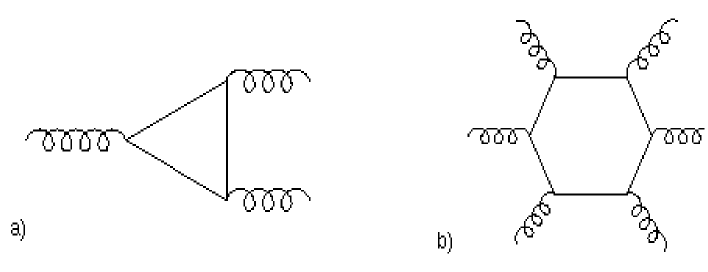
Figure 14: a) The anomalous triangle diagram in four dimensions. b) The anomalous hexagon diagram in ten dimensions.

Anomalies in field theory appear due to UV problems. Consider the famous triangle graph in four dimensions (Fig. 14a). It is superficially linearly divergent, and gauge invariance reduces this to a logarithmic divergence. If the fermions going around the loop are non-chiral, we can regularize the diagram using Pauli-Villars regularization and we can easily show that the graph vanishes when one of the gauge field polarizations is longitudinal. There is no anomaly in this case. However, if the fermions are chiral, Pauli-Villars (or any other regularization) will break gauge invariance, which will not be recovered when the regulator mass is going to infinity.

In ten dimensions, the leading graph that can give a contribution to anomalies is the hexagon diagram depicted in Fig. 14b. The external lines can be either gauge bosons or gravitons. It can be shown that only the completely symmetric part of the graph gives a non-trivial contribution to the anomaly. Non-symmetric contributions can be canceled by local counterterms. If the diagram were non-zero when one of the external lines is longitudinal, then this will imply that the unphysical polarizations will propagate in the two-loop diagram in Fig. 15.

We will consider the linearized approximation, which is relevant for the leading hexagon diagram: $F=F_{0}+A^{2}$, $F_{0}=dA$ and $A\to A+d\Lambda$. Here, $\Lambda$ is the gauge parameter matrix (zero-form). The anomaly due to the hexagon diagram with gauge fields in the external lines can have the following general form

$$\left.\delta\Gamma\right|_{\rm gauge}\sim\int d^{10}x~{}\left[c_{1}{\rm Tr}[\Lambda F_{0}^{5}]+c_{2}{\rm Tr}[\Lambda F_{0}]{\rm Tr}[F_{0}^{4}]+c_{3}{\rm Tr}[\Lambda F_{0}](Tr[F_{0}^{2}])^{2}\right]\,,$$ (11.4)

where powers of forms are understood as wedge products. For comparison, the similar expression in four dimensions is proportional to ${\rm Tr}[\Lambda F_{0}^{2}]$. The three different coefficients $c_{i}$ correspond to the three group invariants ${\rm Tr}[T^{6}]$, ${\rm Tr}[T^{4}]Tr[T^{2}]$ and $({\rm Tr}[T^{2}])^{3}$ of a given group generator $T$ in a symmetric group trace. There is a similar result for the gravitational anomaly, where the role of $F$ is played by the O(D) two-form $R^{ab}_{\mu\nu}=e^{a}_{\rho}e^{b}_{\sigma}{R^{\rho\sigma}}_{\mu\nu}$. The matrix valued two-form $R$ is obtained by multiplying $R^{ab}$ with the O(D) adjoint matrices $T^{ab}$. It can be written in terms of the spin connection one-form $\omega$ as $R=d\omega+\omega^{2}$.

Figure 15: Two-loop diagram with physical external legs in which longitudinal modes propagate.

Considering the anomaly diagram with graviton external lines we obtain

$$\left.\delta\Gamma\right|_{\rm grav}\sim\int d^{10}x~{}\left[d_{1}Tr[\Theta R_{0}^{5}]+d_{2}{\rm Tr}[\Theta R_{0}]{\rm Tr}[R_{0}^{4}]+d_{3}{\rm Tr}[\Theta R_{0}]({\rm Tr}[R_{0}^{2}])^{2}\right]\,.$$ (11.5)

Finally, by considering some of the external lines to be gauge bosons and some to be gravitons we obtain the mixed anomaly

$$\left.\delta\Gamma\right|_{\rm mixed} \sim \int d^{10}x~{}\left[e_{1}{\rm Tr}[\Lambda F_{0}]{\rm Tr}[R_{0}^{4}]+e_{2}{\rm Tr}[\Theta R_{0}]{\rm Tr}[F_{0}^{4}]+\right.$$ (11.6)

$$\left.+e_{3}{\rm Tr}[\Theta R_{0}]({\rm Tr}[F_{0}^{2}])^{2}+e_{4}{\rm Tr}[\Lambda F_{0}]({\rm Tr}[R_{0}])^{2}\right]\,.$$

There is also another potential term ${\rm Tr}[\Lambda F_{0}]{\rm Tr}[F_{0}^{2}]{\rm Tr}[R_{0}^{2}]$, but it can be removed by a local counterterm.

There is a geometric construction that provides the full anomaly from the leading linearized piece (for a more complete discussion see, [5], p. 343). First, the anomaly satisfies the so-called Wess-Zumino consistency condition, which reflects the group structure of gauge transformations. Let $G(\Lambda)=\delta\Gamma/\delta\lambda$. Then

$$\delta_{\Lambda_{1}}G(\Lambda_{2})-\delta_{\Lambda_{2}}G(\Lambda_{1})=G([\Lambda_{1},\Lambda_{2}])\,.$$ (11.7)

The field strengths transform as follows under gauge transformations and diffeomorphisms

$$\delta F=[F,\Lambda]\;\;\;,\;\;\;\delta R=[R,\Theta]\,.$$ (11.8)

It is straightforward to show that the traces ${\rm Tr}[R^{m}]$, ${\rm Tr}[F^{m}]$ are gauge-invariant and closed:

$$d~{}{\rm Tr}[R^{m}]=d~{}{\rm Tr}[F^{m}]=0\,.$$ (11.9)

Also, the traces are non-zero for even $m$. In order to construct the anomaly $D$-form in $D$-dimensions we start with the most general gauge-invariant and closed $(D+2)$-form $I^{D+2}(R,F)$, which can be written as a linear combination of products of even traces of $F,R$. Since $I^{D+2}$ is closed, it can be written (locally) as

$$I^{D+2}(R,F)=d\Omega^{D+1}(\omega,A)\,,$$ (11.10)

where the $(D+1)$-form $\Omega^{D+1}$ is no longer gauge-invariant, but changes under gauge transformations as

$$\delta_{\Lambda}\Omega^{D+1}(\omega,A)=d\Omega^{D}(\omega,A,\Lambda)\,.$$ (11.11)

This is required by the fact that $I^{D+2}$ is gauge-invariant. Finally, the $D$-dimensional anomaly is the piece of $\Omega^{D}$ linear in $\Lambda$.

Except for the irreducible part of the gauge anomaly proportional to ${\rm Tr}\Lambda F_{0}^{5}$ and ${\rm Tr}[\Theta R_{0}^{5}]$, the rest can be canceled, if it appears in a suitable linear combination. This is known as the Green-Schwarz mechanism.

Assume that the reducible part of the anomaly factorizes as follows

$$\left.\delta\Gamma\right|_{\rm reduc} \sim \int d^{10}x~{}\left({\rm Tr}[\Lambda F_{0}]+{\rm Tr}[\Theta R_{0}]\right)\left(a_{1}{\rm Tr}[F_{0}^{4}]+a_{2}{\rm Tr}[R_{0}^{4}]+\right.$$ (11.12)

$$\left.+a_{3}({\rm Tr}[F_{0}^{2}])^{2}+a_{4}({\rm Tr}[R_{0}^{2}])^{2}+a_{5}Tr[F_{0}^{2}]{\rm Tr}[R_{0}^{2}]\right)\,.$$

We have seen that, in N=1 supergravity, the field strength of the antisymmetric tensor is shifted by the gauge Chern-Simons form. We can also add the gravitational Chern-Simons form (it will contribute four derivative terms):

$$\hat{H}=dB+\Omega^{CS}(A)+\Omega^{CS}(\omega)\,.$$ (11.13)

We have also seen that this addition makes the $B$-form transform under gauge transformations and diffeomorphisms to keep $\hat{H}$ invariant. Since

$$\delta_{\Lambda}\Omega^{CS}(A)=d{\rm Tr}[\Lambda dA]\;\;\;,\;\;\;\delta_{\Theta}\Omega^{CS}(\omega)=d{\rm Tr}[\Theta d\omega]$$ (11.14)

the antisymmetric tensor must transform as

$$\delta B=-{\rm Tr}[\Lambda F_{0}+\Theta R_{0}]\,.$$ (11.15)

Thus, the counterterm

$$\Gamma_{\rm counter}\sim\int d^{10}x~{}B~{}\left(a_{1}{\rm Tr}[F_{0}^{4}]+a_{2}{\rm Tr}[R_{0}^{4}]+a_{3}({\rm Tr}[F_{0}^{2}])^{2}+\right.$$ (11.16)

$$\left.+a_{4}({\rm Tr}[R_{0}^{2}])^{2}+a_{5}{\rm Tr}[F_{0}^{2}]{\rm Tr}[R_{0}^{2}]\right)$$

can cancel the reducible anomaly. This mechanism can work also in other dimensions, provided there exists an antisymmetric tensor in the theory. There are also generalizations of this mechanism in theories with more than one antisymmetric tensor. Such theories can be obtained by compactifying superstring theories down to six dimensions.

What kind of fields can contribute to the anomalies? First of all they have to be massless, secondly they must be chiral. Chirality exists in even dimensions, and fields that can be chiral are (spin 1/2) fermions, (spin 3/2) gravitini and (anti)self-dual antisymmetric tensors $B_{\mu_{1}\dots\mu_{D/2-1}}$. Their field strength $F=dB$ is a $D/2$-form that is (anti)self-dual

$$F_{\mu_{1}\dots\mu_{D/2}}=\pm{i\over(D/2)!}\epsilon_{\mu_{1}\dots\mu_{D}}F^{\mu_{D/2+1}\dots\mu_{D}}\,.$$ (11.17)

For gravitational anomalies to appear, we must have chiral representations of the Lorentz group O(1,D-1). They exist in $D=4k+2$ dimensions. For gauge anomalies, we must have chiral representations of the gauge group G. This can happen in even dimensions and when the gauge group admits complex representations.

We will now give the contributions to the anomalies coming from the various chiral fields. As we argued before, the anomaly is completely characterized by a closed, gauge-invariant (D+2)-form. By an orthogonal transformation we can bring the $D\times D$ antisymmetric matrix $R_{0}$ to the following block-diagonal form

$$R_{0}=\left(\matrix{0&x_{1}&0&0&&\dots&\cr-x_{1}&0&0&0&&\dots&\cr 0&0&0&x_{2}&&\dots&\cr 0&0&-x_{2}&0&&\dots&\cr&\dots&\dots&\dots&\dots&\dots&\cr&\dots&&&&0&x_{D/2}\cr&\dots&&&&-x_{D/2}&0\cr}\right)\,.$$ (11.18)

Then ${\rm Tr}[R_{0}^{2m}]=2(-1)^{m}\sum_{i}x_{i}^{2m}$. The contribution to the gravitational anomaly of a spin ${\textstyle{1\over 2}}$ fermion is given by [34]

$$\hat{I}_{1/2}(R)=\prod_{i=1}^{D/2}\left({x_{i}/2\over\sinh(x_{i}/2)}\right)\,.$$ (11.19)

In the previous formula, we have to expand it in a series that contains forms of various orders and pick the piece that is a (D+2)-form. Similarly, we have the following contributions for chiral gravitini:

$$I_{3/2}(R)=\hat{I}_{1/2}(R)\left(-1+2\sum_{i=1}^{D/2}\cosh(x_{i})\right)$$ (11.20)

and self-dual tensors

$$I_{A}(R)=-{1\over 8}\prod_{i=1}^{D/2}\left({x_{i}\over\tanh(x_{i})}\right)\,.$$ (11.21)

The gravitini and self-dual tensors do not contribute to gauge or mixed anomalies, since they cannot be charged under the gauge group. However the spin 1/2 fermions can transform non-trivially and their total contribution to anomalies is given by

$$I_{1/2}(R,F)=Tr\left[e^{iF}\right]\hat{I}_{1/2}(R)\,.$$ (11.22)

Assuming $D=10$ and expanding the formulae above we obtain

$$\left.I_{1/2}(R,F)\right|_{\rm 12-form} = -{{\rm Tr}[F^{6}]\over 720}+{Tr[F^{4}]Tr[R^{2}]\over 24\cdot 48}+$$

$$-{Tr[F^{2}]\over 256}\left({Tr[R^{4}]\over 45}+{(Tr[R^{2}])^{2}\over 36}\right)+$$

$$+{n\over 64}\left({Tr[R^{6}]\over 5670}+{Tr[R^{2}]Tr[R^{4}]\over 4320}+{(Tr[R^{2}])^{3}\over 10368}\right)\,,$$

where $n$ is the total number of spin 3/2 fermions.

$$\left.I_{3/2}(R)\right|_{\rm 12-form} = -{495\over 64}\left({Tr[R^{6}]\over 5670}+{Tr[R^{2}]Tr[R^{4}]\over 4320}+{(Tr[R^{2}])^{3}\over 10368}\right)+$$

$$+{Tr[R^{2}]\over 384}\left(Tr[R^{4}]+{(Tr[R^{2}])^{2}\over 4}\right)\,,$$

$$\left.I_{A}(R)\right|_{\rm 12-form}=\left.\hat{I}_{1/2}(R)\right|_{\rm 12-form}-\left.I_{3/2}(R)\right|_{\rm 12-form}\,.$$ (11.23)

The anomaly contributions $I_{1/2}$ and $I_{3/2}$ given above correspond to Weyl fermions. Since in ten dimensions we also have Majorana-Weyl fermions, their contribution to anomalies is half of the above.

We are now in a position to examine which ten-dimensional theories are free of anomalies.

The theory of N=1 supergravity without matter contains a Majorana-Weyl gravitino and a Majorana-Weyl spin ${\textstyle{1\over 2}}$ fermion of opposite chirality. It can easily be checked from the formulae above that this is anomalous.

Type-IIA supergravity is non-chiral and thus trivially anomaly-free. Type-IIB, however, is chiral and contains two Majorana-Weyl gravitini contributing $I_{3/2}$ to the anomaly, two Majorana-Weyl fermions of the opposite chirality contributing $-I_{1/2}$, and a self-dual tensor contributing $-I_{A}$. The total anomaly can be seen to vanish from (11.23).

We will now consider N=1 supergravity coupled to vector multiplets. The gaugini have the same chirality as the gravitino. The total anomaly is

$$2I^{N=1}=I_{3/2}(R)-I_{1/2}(R)+I_{1/2}(R,F)\,.$$ (11.24)

We should at least require that the irreducible anomaly corresponding to the traces of $R^{6}$ and $F^{6}$ cancels. The ${\rm Tr}[R^{6}]$ cannot be written as a product of lower traces, since the group O(10) has an independent Casimir of order 6. Thus, the coefficient of the ${\rm Tr}[R^{6}]$ term in (11.24) must vanish. This implies that $n=496$. Since the gaugini are in the adjoint representation of the gauge group, their number $n$ is the dimension of the gauge group. We obtain that a necessary (but not sufficient) condition for anomaly cancelation is $\mbox{dim}G=496$. Inserting $n=496$ in (11.24) we obtain

$$96I^{\rm total}=-{{\rm Tr}[F^{6}]\over 15}+{{\rm Tr}[R^{2}]{\rm Tr}[F^{4}]\over 24}+{{\rm Tr}[R^{2}]{\rm Tr}[R^{4}]\over 8}+{({\rm Tr}[R^{2}])^{3}\over 32}-$$ (11.25)

$$-{{\rm Tr}[F^{2}]\over 960}\left(4{\rm Tr}[R^{4}]+5({\rm Tr}[R^{2}])^{2}\right)\,.$$

It is obvious from the above that the only hope for canceling the leftover anomaly is to be able to use the Green-Schwarz mechanism. It would work if we could factorize $I^{\rm total}$. This will happen iff

$${\rm Tr}[F^{6}]={1\over 48}{\rm Tr}[F^{2}]{\rm Tr}[F^{4}]-{1\over 14400}({\rm Tr}[F^{2}])^{3}\,.$$ (11.26)

Then

$$96I^{\rm total}=\left({\rm Tr}[R^{2}]-{1\over 30}{\rm Tr}[F^{2}]\right)~{}X_{8}\,,$$ (11.27)

with

$$X_{8}={{\rm Tr}[F^{4}]\over 24}-{({\rm Tr}[F^{2}])^{2}\over 720}-{{\rm Tr}[F^{2}]{\rm Tr}[R^{2}]\over 240}+{{\rm Tr}[R^{4}]\over 8}+{({\rm Tr}[R^{2}])^{2}\over 32}\;,$$ (11.28)

and the rest of the anomaly can be canceled via the Green-Schwarz mechanism. The only non-trivial condition that remains is (11.26).

Consider first the gauge group to be O(N). Then the following formulae apply [5]

$${\rm Tr}[F^{6}]=(N-32){\rm tr}[F^{6}]+15{\rm tr}[F^{2}]{\rm tr}[F^{4}]\,,$$ (11.29)

$${\rm Tr}[F^{4}]=(N-8){\rm tr}[F^{4}]+3({\rm tr}[F^{2}])^{2}\;\;\;,\;\;\;{\rm Tr}[F^{2}]=(N-2){\rm tr}[F^{2}]\,,$$ (11.30)

where Tr stands for the trace in the adjoint and tr for the trace in the fundamental of O(N).

Exercise. Show that the factorization condition (11.26) and $\mbox{dim}G=496$ are satisfied by G=O(32). Thus, the type-I and heterotic string theories with G=O(32) are anomaly free.

Consider now $\rm G=E_{8}\times E_{8}$, which has also dimension 496. $\rm E_{8}$ has no independent Casimirs of order 4 and 6,

$${\rm Tr}[F^{6}]={1\over 7200}({\rm Tr}[F^{2}])^{3}\;\;\;,\;\;\;{\rm Tr}[F^{4}]={1\over 100}({\rm Tr}[F^{2}])^{2}\,.$$ (11.31)

Exercise. Verify that $\rm E_{8}\times E_{8}$ satisfies (11.26). Thus, the E${}_{8}\times$E₈ heterotic string is also anomaly-free. Check also that the groups E${}_{8}\times$U(1)²⁴⁸ and U(1)⁴⁹⁶ are anomaly-free. No known ten-dimensional string theory corresponds to these groups.

The presence of the Green-Schwarz counterterm (11.16) necessary for the cancelation of the reducible anomaly, was checked by a one-loop computation in the heterotic string [35]. Moreover a direct relation between modular invariance and the absence of anomalies was obtained.

From (11.13) we obtain that (G=O(32))

$$d\hat{H}={\rm tr}[R^{2}]-{1\over 30}{\rm Tr}[F^{2}]\,.$$ (11.32)

Integrating (11.24) over any closed four-dimensional submanifold, we obtain the important constraint to be satisfied by the background fields:

$$\int~{}{\rm tr}[R^{2}]={1\over 30}\int~{}{\rm Tr}[F^{2}]\,.$$ (11.33)

Exercise. Consider the non-supersymmetric $\rm O(16)\times O(16)$ heterotic string in ten dimensions. It is a chiral theory with fermionic content transforming as $(V,V)$, $(\bar{S},1)$ and $(1,\bar{S})$ under the gauge group. $S$ stands for the 128-dimensional spinor representation of O(16). Use

$${\rm tr}_{S}[F^{6}]=16{\rm tr}[F^{6}]-15{\rm tr}[F^{2}]{\rm tr}[F^{4}]+{15\over 4}({\rm tr}[F^{2}])^{3}\,,$$ (11.34)

$${\rm tr}_{S}[F^{4}]=-8{\rm tr}[F^{4}]+6({\rm tr}[F^{2}])^{2}\;\;\;,\;\;\;{\rm tr}_{S}[F^{2}]=16{\rm tr}[F^{2}]\,,$$ (11.35)

with tr_S the trace in the spinor representation space and tr the trace in the fundamental representation space to show that the theory is anomaly-free. What is the Green-Schwarz counterterm? Are there any other chiral, non-supersymmetric anomaly-free theories in ten dimensions?

Exercise. Consider the $\rm E_{8}\times E_{8}$ heterotic string in ten dimensions. This theory has a symmetry ${\cal I}$ that interchanges the two $\rm E_{8}$ factors. Consider the $Z_{2}$ orbifold of this theory with respect to the symmetry transformation $g=(-1)^{F+1}\cdot{\cal I}$. Construct the modular-invariant partition function (you will need the duplication formulae for the $\vartheta$-functions that you can find in appendix A). What is the gauge group and the massless spectrum? Is this theory supersymmetric? Chiral? Anomaly-free?

12 Compactification and supersymmetry breaking

So far, we have considered superstring theories in ten non-compact dimensions. However, our direct physical interest is in four-dimensional theories. One way to obtain them is to make use of the Kaluza-Klein idea: consider some of the dimensions to be curled-up into a compact manifold, leaving only four non-compact dimensions. As we have seen in the case of the bosonic strings, exact solutions to equations of motion of a string theory correspond to a CFT. In the case of type-II string theory, they would correspond to a (1,1) superconformal FT, and to a (1,0) superconformal FT in the heterotic case. The generalization of the concept of compactification to four dimensions, for example, is to replace the original flat non-compact CFT with another one, where four dimensions are still flat but the rest is described by an arbitrary CFT with the appropriate central charge. This type of description is more general than that of a geometrical compactification, since there are CFTs with no geometrical interpretation. In the following, we will examine both the geometric point of view and the CFT point of view, mainly via orbifold compactifications.

12.1 Toroidal compactifications

The simplest possibility is that the “internal compact” manifold be a flat torus. This can be considered as a different background of the ten-dimensional theory, where we have given constant expectation values to internal metric and other background fields.

Consider first the case of the heterotic string compactified to $D<10$ dimensions. It is rather straightforward to construct the partition function of the compactified theory. There are now $D-2$ transverse non-compact coordinates, each contributing $\sqrt{\tau_{2}}\eta\bar{\eta}$. There is no change in the contribution of the left-moving world-sheet fermions and 16 right-moving compact coordinates. Finally the contribution of the $10-D$ compact coordinates is given by (7.1.38). Putting everything together we obtain

$$Z^{\rm heterotic}_{D}={\Gamma_{10-D,10-D}(G,B)~{}\bar{\Gamma}_{H}\over\tau_{2}^{D-2\over 2}\eta^{8}\bar{\eta}^{8}}~{}{1\over 2}\sum_{a,b=0}^{1}~{}(-1)^{a+b+ab}~{}{\vartheta^{4}[^{a}_{b}]\over\eta^{4}}\,,$$ (12.1.1)

where $\bar{\Gamma}_{H}$ stands for the lattice sum for either O(32) or $\rm E_{8}\times E_{8}$; $G_{\alpha\beta}$, $B_{\alpha\beta}$ are the constant expectation values of the internal $(10-D)$-dimensional metric and antisymmetric tensor. It is not difficult to find the massless spectrum of the theory. The original ten-dimensional metric gives rise to the $D$-dimensional metric, $(10-D)$ U(1) gauge fields and ${\textstyle{1\over 2}}(10-D)(11-D)$ scalars. The antisymmetric tensor produces a $D$-dimensional antisymmetric tensor, $(10-D)$ $U(1)$ gauge fields and ${\textstyle{1\over 2}}(10-D)(9-D)$ scalars (the internal components of the gauge fields). The ten-dimensional dilaton gives rise to another scalar. Finally the dim $H$ ten-dimensional gauge fields give rise to dim $H$ gauge fields and $(10-D)\cdot$ dim $H$ scalars. Similar reduction works for the fermions.

We will consider in more detail the scalars $Y^{a}_{\alpha}$ coming from the ten-dimensional vectors, where $a$ is the adjoint index and $\alpha$ the internal index taking values $1,2,\dots,10-D$. The non-abelian field strength (10.6.3) contains a term without derivatives. Upon dimensional reduction this gives rise to a potential term for the (Higgs) scalars $Y^{a}_{\alpha}$:

$$V_{\rm Higgs}\sim{f^{a}}_{bc}{f^{a}}_{b^{\prime}c^{\prime}}~{}G^{\alpha\gamma}~{}G^{\beta\delta}~{}Y_{\alpha}^{b}~{}Y_{\beta}^{c}~{}Y_{\gamma}^{b^{\prime}}~{}Y^{c^{\prime}}_{\delta}\,.$$ (12.1.2)

This potential has flat directions (continuous families of minima) when $Y^{a}_{\alpha}$ takes constant expectation values in the Cartan subalgebra of the Lie algebra. We will label these values by $Y^{I}_{\alpha}$, $I=1,2,\dots,16$. This is a normal Higgs phenomenon and it generates a mass matrix for the gauge fields

$$\left[m^{2}\right]^{ab}\sim G^{\alpha\beta}~{}{f^{ca}}_{d}~{}{f^{cb}}_{d}^{\prime}~{}Y^{d}_{\alpha}~{}Y^{d^{\prime}}_{\beta}\,.$$ (12.1.3)

This mass matrix has rank-H generic zero eigenvalues. The gauge fields belonging to the Cartan remain massless while all the other gauge fields get a non-zero mass. Consequently, the gauge group is broken to the Cartan $\sim\rm U(1)^{{\rm rank}-H}$. If we also turn on these expectation values, then the heterotic compactified partition function becomes

$$Z^{\rm heterotic}_{D}={\Gamma_{10-D,26-D}(G,B,Y)\over\tau_{2}^{D-2\over 2}\eta^{8}\bar{\eta}^{8}}~{}{1\over 2}\sum_{a,b=0}^{1}~{}(-1)^{a+b+ab}~{}{\vartheta^{4}[^{a}_{b}]\over\eta^{4}}\,,$$ (12.1.4)

where the derivation of the $\Gamma_{10-D,26-D}$ lattice sum is described in detail in Appendix B.

The $(10-D)(26-D)$ scalar fields $G,B,Y$ are called moduli since they can have arbitrary expectation values. Thus, the heterotic string compactified down to $D$ dimensions is essentially a continuous family of $vacua$ parametrized by the expectation values of the moduli that describe the geometry of the internal manifold $(G,B)$ and the (flat) gauge bundle ($Y$).

Consider now the tree-level effective action for the bosonic massless modes in the toroidally compactified theory. It can be obtained by direct dimensional reduction of the ten-dimensional heterotic effective action, which in the $\sigma$-model frame is given by (9.10) with the addition of the gauge fields

$$\alpha^{\prime 8}~{}S_{10-d}^{\rm heterotic}=\int d^{10}x\sqrt{-{\rm det}~{}G_{10}}e^{-\Phi}\left[R+(\nabla\Phi)^{2}-{1\over 12}\hat{H}^{2}-{1\over 4}{\rm Tr}[F^{2}]\right]+{\cal O}(\alpha^{\prime})\,.$$ (12.1.5)

The massless fields in $D$ dimensions are obtained from those of the ten-dimensional theory by assuming that the latter do not depend on the internal coordinates $X^{\alpha}$. Moreover we keep only the Cartan gauge fields since they are the only ones that will remain massless for generic values of the Wilson lines $Y^{I}_{\alpha}$, $I=1,2,\dots,16$. So, the gauge kinetic terms abelianize ${\rm Tr}[F^{2}]\to\sum_{I=1}^{16}F^{I}_{\mu\nu}F^{I,\mu\nu}$ with

$$F^{I}_{\mu\nu}=\partial_{\mu}A^{I}_{\nu}-\partial_{\nu}A^{I}_{\mu}\,.$$ (12.1.6)

Also

$$\hat{H}_{\mu\nu\rho}=\partial_{\mu}B_{\nu\rho}-{1\over 2}\sum_{I}A^{I}_{\mu}F^{I}_{\nu\rho}+{\rm cyclic}\,,$$ (12.1.7)

where we have neglected the gravitational Chern-Simons contribution, since it is of higher order in $\alpha^{\prime}$.

There is a standard ansatz to define the $D$-dimensional fields, such that the gauge invariances of the compactified theory are simple. This is given in Appendix C. In this way we obtain

$$S^{\rm heterotic}_{D}=\int~{}d^{D}x~{}\sqrt{-{\rm det}~{}G}e^{-\Phi}\left[R+\partial^{\mu}\Phi\partial_{\mu}\Phi-{1\over 12}\hat{H}^{\mu\nu\rho}\hat{H}_{\mu\nu\rho}-\right.$$

$$\left.-{1\over 4}(\hat{M}^{-1})_{ij}F^{i}_{\mu\nu}F^{j\mu\nu}+{1\over 8}{\rm Tr}(\partial_{\mu}\hat{M}\partial^{\mu}\hat{M}^{-1})\right]\,,\quad\quad$$ (12.1.8)

where $i=1,2,\dots,36-2D$ and

$$\hat{H}_{\mu\nu\rho}=\partial_{\mu}B_{\nu\rho}-{1\over 2}L_{ij}A^{i}_{\mu}F^{j}_{\nu\rho}+{\rm cyclic}\,.$$ (12.1.9)

The moduli scalar matrix $\hat{M}$ is given in (B.4). This action has a continuous O(10-D,26-D) symmetry. If $\Lambda\in$ O(10-D,26-D) is a $(36-2D)\times(36-2D)$ matrix then

$$\hat{M}\to\Omega~{}\hat{M}~{}\Omega^{T}\;\;\;,\;\;\;A_{\mu}\to\Omega\cdot A_{\mu}$$ (12.1.10)

leaves the effective action invariant. However, we know from the exact string theory treatment that the presence of the massive states coming from the lattice break this symmetry to the discrete infinite subgroup O(10-D,26-D,$\hbox{\mybb Z})$. This is the group of T-duality symmetries. The $(10-D)(26-D)$ scalar action in (12.1.8) is the $\rm O(10-D,26-D)/(O(10-D)\times O(26-D)$ $\sigma$-model.

We can also go to the Einstein frame by (9.11), in which the action becomes

$$S^{\rm heterotic}_{D}=\int~{}d^{D}x~{}\sqrt{-{\rm det}~{}G_{E}}\left[R-{1\over D-2}\partial^{\mu}\Phi\partial_{\mu}\Phi-{e^{-{4\Phi\over D-2}}\over 12}\hat{H}^{\mu\nu\rho}\hat{H}_{\mu\nu\rho}-\right.$$

$$\left.-{e^{-{2\Phi\over D-2}}\over 4}(\hat{M}^{-1})_{ij}F^{i}_{\mu\nu}F^{j\mu\nu}+{1\over 8}Tr(\partial_{\mu}\hat{M}\partial^{\mu}\hat{M}^{-1})\right]\,.\quad\quad\quad\quad$$ (12.1.11)

For $D=4$, the ten-dimensional gravitino gives rise to 4 four-dimensional Majorana gravitini. Consequently, the four-dimensional compactified theory has N=4 local SUSY. The relevant massless N=4 supermultiplets are the supergravity multiplet and the vector multiplet. The supergravity multiplet contains the metric, six vectors (the graviphotons), a scalar and an antisymmetric tensor, as well as four Majorana gravitini and four Majorana spin ${\textstyle{1\over 2}}$ fermions. The vector multiplet contains a vector, four Majorana spin ${\textstyle{1\over 2}}$ fermions and six scalars. In total we have, apart from the SUGRA multiplet, 22 vector multiplets.

In $D=4$ the antisymmetric tensor is equivalent (on-shell) via a duality transformation to a pseudoscalar $a$, the “axion”. It is defined (in the Einstein frame) by

$$e^{-2\phi}\hat{H}_{\mu\nu\rho}={{\epsilon_{\mu\nu\rho}}^{\sigma}\over\sqrt{-{\rm det}~{}g_{E}}}\nabla_{\sigma}a\,.$$ (12.1.12)

This definition is such that the $B_{\mu\nu}$ equations of motion $\nabla^{\mu}e^{-\Phi}\hat{H}_{\mu\nu\rho}=0$ are automatically solved by substituting (12.1.12). However the Bianchi identity for $\hat{H}$ from (12.1.9)

$${\epsilon^{\mu\nu\rho\sigma}\over\sqrt{-{\rm det}~{}g_{E}}}\partial_{\mu}\hat{H}_{\nu\rho\sigma}=-L_{ij}F^{i}_{\mu\nu}\tilde{F}^{j,\mu\nu}\,,$$ (12.1.13)

where

$$\tilde{F}^{\mu\nu}={1\over 2}{\epsilon^{\mu\nu\rho\sigma}\over\sqrt{-{\rm det}~{}g_{E}}}F_{\rho\sigma}\;,$$ (12.1.14)

becomes, after substituting (12.1.12), an equation of motion for the axion:

$$\nabla^{\mu}~{}e^{2\phi}\nabla_{\mu}a=-{1\over 4}F^{i}_{\mu\nu}\tilde{F}^{j,\mu\nu}\,.$$ (12.1.15)

This equation can be obtained from the “dual” action

$$\tilde{S}^{\rm heterotic}_{D=4}=\int d^{4}x\sqrt{-{\rm det}~{}g_{E}}\;\left[R-{1\over 2}\partial^{\mu}\phi\partial_{\mu}\phi-{1\over 2}e^{2\phi}\partial^{\mu}a\partial_{\mu}a+\right.$$

$$\left.-{1\over 4}e^{-\phi}(M^{-1})_{ij}F^{i}_{\mu\nu}F^{j,\mu\nu}+{1\over 4}a\;L_{ij}F^{i}_{\mu\nu}\tilde{F}^{j,\mu\nu}+\right.$$

$$\left.+{1\over 8}{\rm Tr}(\partial_{\mu}M\partial^{\mu}M^{-1})\right]\,.\quad\quad$$ (12.1.16)

Finally defining the complex $S$ field

$$S=a+i\;e^{-\phi}\;,$$ (12.1.17)

we can write the action as

$$\tilde{S}^{\rm heterotic}_{D=4}=\int d^{4}x\sqrt{-{\rm det}~{}g_{E}}\;\left[R-{1\over 2}{\partial^{\mu}S\partial_{\mu}\bar{S}\over{\rm Im}S^{2}}-{1\over 4}{\rm Im}S(M^{-1})_{ij}F^{i}_{\mu\nu}F^{j,\mu\nu}\right.$$

$$\left.+{1\over 4}{\rm Re}S\;L_{ij}F^{i}_{\mu\nu}\tilde{F}^{j,\mu\nu}+{1\over 8}{\rm Tr}(\partial_{\mu}M\partial^{\mu}M^{-1})\right]\;.\quad\quad\quad$$ (12.1.18)

From the definition (12.1.17), $1/{\rm Im}S$ is the string loop-expansion parameter (heterotic string coupling constant). As we will see later on, the 4-d heterotic string has a non-perturbative SL(2,$\hbox{\mybb Z})$ symmetry acting on $S$ by fractional transformations and as electric-magnetic duality on the abelian gauge fields. The scalar field $S$ takes values in the upper-half plane, SL(2,ℝ)/U(1). The rest of the scalars take values in the coset space O(6,22)/O(6)$\times$O(22).

We will briefly describe here the toroidal compactification of type-II string theory to four dimensions. It can be shown that in closed string theory with a compact dimension of radius $R$, a duality transformation $R\to 1/R$ is accompanied by a reversal of the chirality of the left-moving spinor groundstate. This is explained in more detail in the last section. Thus, type-IIA theory with radius $R$ is equivalent to type-IIB theory with radius $1/R$. Once we compactify on a torus, both theories are non-chiral. We need only examine the type-IIA theory reduction to $D=4$. First the two Majorana-Weyl gravitini and fermions give rise to eight $D=4$ Majorana gravitini and 48 spin ${\textstyle{1\over 2}}$ Majorana fermions. Thus, the $D=4$ theory has maximal N=8 supersymmetry. The ten-dimensional metric produces the four-dimensional metric, 6 U(1) vectors and 21 scalars. The antisymmetric tensor produces (after four-dimensional dualization), 6 U(1) vectors and 16 scalars. The dilaton gives an extra scalar. The $R$-$R$ U(1) gauge field gives one gauge field and 6 scalars. The $R$-$R$ three-form gives a three-form (no physical degrees of freedom in four dimensions) 15 vectors and 26 scalars. All of the above degrees of freedom form the N=8 supergravity multiplet that contains the graviton, 28 vectors, 70 scalars, 8 gravitini and 48 fermions.

Exercise. Start from the ten-dimensional type-IIA effective action in (10.6.19) and by using toroidal dimensional reduction (you will find relevant formulae in appendix C) derive the four-dimensional effective action. Dualize all two-forms.

12.2 Compactification on non-trivial manifolds

The next step would be to attempt to compactify the ten-dimensional theories on non-flat manifolds. Such backgrounds, however, must satisfy the string equations of motion. As we described in a previous section, this is equivalent to conformal invariance of the associated $\sigma$-model. When the background fields are slowly varying, the $\alpha^{\prime}$ expansion is applicable and to leading order the background must satisfy the low-energy effective field equations of motion.

We will be interested in ground-states for which the four-dimensional world is flat. In the most general case, such a ground-state is given by the tensor product of a four-dimensional non-compact flat CFT and an internal conformal field theory. A CFT with appropriate central charge and symmetries is an exact solution of the (tree-level) string equations of motion to all orders in $\alpha^{\prime}$. In the heterotic case, this internal CFT must have left N=1 invariance and $(c,\bar{c})=(9,22)$. In the type-II case it must have both left and right N=1 superconformal invariance and $(c,\bar{c})=(9,9)$. If the CFT has a “large volume limit”, then an $\alpha^{\prime}$ expansion is possible and we can recover the leading $\sigma$-model (geometrical) results.

It is also of interest, for the compactified theory, to have some left-over supersymmetry at the compactification scale. For phenomenological purposes we eventually need N=1 supersymmetry, since it is the only case that admits chiral representations. Although the very low energy world is not supersymmetric, we do need some supersymmetry beyond Standard-Model energies for hierarchy reasons.

In the effective field theory approach, we assume that some bosonic fields acquire expectation values that satisfy the equations of motion, while the expectation values of the fermions are zero (to preserve $D=4$ Lorentz invariance). In the generic case, a background breaks all the supersymmetries of flat ten-dimensional space. A supersymmetry will be preserved, if the associated variation of the fermion fields vanish. This gives a set of first order equations. If they are satisfied for at least one supersymmetry, then the full equations of motion will also be satisfied. Another way to state this is by saying that every compact manifold that preserves at least one SUSY, is a solution of the equations of motion.

We will consider here the case of the heterotic string on a space that is locally $M_{4}\times K$ with $M_{4}$ the four-dimensional Minkowski space and $K$ some six-dimensional compact manifold. Splitting indices into Greek indices for $M_{4}$ and Latin indices for $K$, we have the following supersymmetry variations (in the Einstein frame) of the ten-dimensional heterotic action

$$\delta\psi_{\mu}=\nabla_{\mu}\epsilon+{\sqrt{2}\over 32}e^{2\Phi}\left(\gamma_{\mu}\gamma_{5}\otimes H\right)\epsilon\,,$$ (12.2.1)

$$\delta\psi_{m}=\nabla_{m}\epsilon+{\sqrt{2}\over 32}e^{2\Phi}\left(\gamma_{m}H-12H_{m}\right)\epsilon\,,$$ (12.2.2)

$$\delta\lambda=\sqrt{2}(\gamma^{m}\nabla_{m}\Phi)\epsilon+{1\over 8}e^{2\Phi}H\epsilon\,,$$ (12.2.3)

$$\delta\chi^{a}=-{1\over 4}e^{\Phi}F^{a}_{m,n}\gamma^{mn}\epsilon\,,$$ (12.2.4)

where $\psi$ is the gravitino, $\lambda$ is the dilatino and $\chi^{a}$ are the gaugini; $\epsilon$ is a spinor (the parameter of the supersymmetry transformation). Furthermore we used

$$H=H_{mnr}~{}\gamma^{mnr}\;\;\;,\;\;\;H_{m}=H_{mnr}~{}\gamma^{nr}\,.$$ (12.2.5)

The ten-dimensional $\Gamma$-matrices can be constructed from the $D=4$ matrices $\gamma^{\mu}$, and the internal matrices $\gamma^{m}$, as

$$\Gamma^{\mu}=\gamma^{\mu}\otimes{\bf 1}_{6}\;\;\;,\;\;\;\Gamma^{m}=\gamma^{5}\otimes\gamma^{m}\,,$$ (12.2.6)

$$\gamma^{5}={i\over 4!}\epsilon_{\mu\nu\rho\sigma}\gamma^{\mu\nu\rho\sigma}\;\;\;,\;\;\;\gamma={i\over 6!}\sqrt{\rm detg}\epsilon_{mnrpqs}\gamma^{mnrpqs}\;.$$ (12.2.7)

$\gamma$ is the analog of $\gamma^{5}$ for the internal space.

If, for some value of the background fields, the equations $\delta({\rm fermions})=0$ admit a solution, namely a non-trivial, globally defined spinor $\epsilon$, then the background is N=1 supersymmetric. If more than one solution exist, then we will have extended supersymmetry. This problem was considered in [36] with the assumption that $H_{mnr}=0$. The conditions for the existence of N=1 supersymmetry in four dimensions for $H=0$ can be summarized as follows: the dilaton must be constant and the manifold $K$ must admit a Killing spinor $\xi$,

$$\nabla_{m}~{}\xi=0\,.$$ (12.2.8)

Moreover this condition implies that $K$ is a Ricci-flat ($R_{mn}=0$) Kähler manifold. Finally the background (internal) gauge fields must satisfy

$$F^{a}_{mn}\gamma^{mn}~{}\xi=0$$ (12.2.9)

and (11.32) then becomes

$${R^{rs}}_{[mn}R_{pq]rs}={1\over 30}F^{a}_{[mn}F^{a}_{pq]}\,.$$ (12.2.10)

In a generic six-dimensional manifold, the spin connection is in $\rm O(6)\sim SU(4)$. If the manifold is Kähler, then the spin connection is in $\rm U(3)\subset SU(4)$. Finally, if the Ricci tensor vanishes, the spin connection is an SU(3) connection. Such manifolds are known as Calabi-Yau (CY) manifolds.

A simple way to solve (12.2.9) and (12.2.10) is to embed the spin connection $\omega\in\rm SU(3)$ into the gauge connection $A\in\rm O(32)$ or $\rm E_{8}\times E_{8}$. The only embedding of SU(3) in O(32) that satisfies (12.2.10) is the one in which $\rm O(32)\ni 32\to 3+\bar{3}+{\rm singlets}\in SU(3)$. In this case O(32) is broken down to $\rm U(1)\times O(26)$ (this is the subgroup that commutes with SU(3)). The U(1) is “anomalous”, namely the sum of the U(1) charges $\rho=\sum_{i}q^{i}$ of the massless states is not zero. This anomaly is apparent, since we know that the string theory is not anomalous. What happens is that the Green-Schwarz mechanism implies here that there is a one-loop coupling of the form $\rho~{}B\wedge F$. This gives a mass to the U(1) gauge field and it cannot appear as a low-energy symmetry. There is a more detailed discussion of this phenomenon in section 13.4. The leftover gauge group O(26) has only non-chiral representations.

More interesting is the case of $\rm E_{8}\times E_{8}$. $\rm E_{8}$ has a maximal $\rm SU(3)\times E_{6}$ subgroup, under which the adjoint of $\rm E_{8}$ decomposes as $\rm E_{8}\ni{\bf 248}\to({\bf 8,1})\otimes({\bf 3,27})\otimes({\bf\bar{3},\overline{27}})\otimes({\bf 1,78})\in SU(3)\times E_{6}$. Embedding the spin connection in one of the $\rm E_{8}$ in this fashion solves (12.2.10). The unbroken gauge group in this case is $\rm E_{6}\times E_{8}$. Let $N_{L}$ be the number of massless left-handed Weyl fermions in four dimensions transforming in the $\bf 27$ of $\rm E_{6}$ and $N_{R}$ the same number for the $\bf\overline{27}$. The number of net chirality (number of “generations”) is $|N_{L}-N_{R}|$; it can be obtained by an index theorem on the CY manifold. The $\bf 27$’s transform as the $\bf 3$ of SU(3) and the $\bf\overline{27}$ transform in the $\bf\bar{3}$ of SU(3). Thus, the number of generations is the index of the Dirac operator on $K$ for the fermion field $\psi_{\alpha A}$, where $\alpha$ is a spinor index and $A$ is a $\bf 3$ index. It can be shown [36], that the index of the Dirac operator, and thus the number of generations, is equal to $|\chi(K)/2|$, where $\chi(K)$ is the Euler number of the manifold $K$.

The above considerations are correct to leading order in $\alpha^{\prime}$. At higher orders we expect, generically, corrections and only some statements about the massless states survive these corrections.

As another example we will consider the compactification of type-II theory on the K3 manifold down to six dimensions. K3 is a topological class of four-dimensional compact, Ricci-flat, Kähler manifolds without isometries. Such manifolds have SU(2)$\subset$O(4) holonomy and are also hyper-Kähler. The hyper-Kähler condition is equivalent to the existence of three integrable complex structures that satisfy the SU(2) algebra. It can be shown that a left-right symmetric N=1 supersymmetric $\sigma$-model on such manifolds is exactly conformally invariant and has N=4 superconformal symmetry on both sides. Moreover, K3 has a covariantly constant spinor, so that the type-II theory compactified on it has N=2 supersymmetry in six dimensions (and N=4 if further compactified on a two-torus). It would be useful for latter purposes to briefly describe the cohomology of K3. There is a harmonic zero-form that is constant (since the manifold is compact and connected). There are no harmonic one-forms. There is one (2,0) and one (0,2) harmonic forms as well as 20 (1,1) forms. The (2,0), (0,2) and one of the (1,1) Kähler forms are self-dual, the other 19 (1,1) forms are anti-self-dual. There are no harmonic three-forms and a unique four-form (the volume form). More details on the geometry and topology of K3 can be found in [37].

Consider first the type-IIA theory and derive the massless bosonic spectrum in six dimensions. To find the massless states coming from the ten-dimensional metric $G$, we make the following decomposition

$$G_{MN}\sim h_{\mu\nu}(x)\otimes\phi(y)+A_{\mu}(x)\otimes f_{m}(y)+\Phi(x)\otimes h_{mn}(y)\,,$$ (12.2.11)

where $x$ denotes the six-dimensional non-compact flat coordinates and $y$ are the internal coordinates. Also $\mu=0,1,\dots,5$ and $m=1,2,3,4$ is a K3 index. Applying the ten-dimensional equations of motion to the metric $G$ we obtain that $h_{\mu\nu}$ (the six-dimensional graviton) is massless if

$$\hbox{{$\sqcup$}\hbox to0.0pt{\hss$\sqcap$}}_{y}~{}\phi(y)=0\,.$$ (12.2.12)

The solutions to this equation are the harmonic zero-forms, and there is only one of them. Thus, there is one massless graviton in six dimensions. $A_{\mu}(x)$ is massless if $f_{m}(y)$ is covariantly constant on K3. Thus, it must be a harmonic one-form and there are none on K3. Consequently, there are no massless vectors coming from the metric. $\Phi(x)$ is a massless scalar if $h_{mn}(y)$ satisfies the Lichnerowicz equation

$$-\hbox{{$\sqcup$}\hbox to0.0pt{\hss$\sqcap$}}h_{mn}+2R_{mnrs}h^{rs}=0\;\;\;,\;\;\;\nabla^{m}h_{mn}=g^{mn}h_{mn}=0\,.$$ (12.2.13)

The solutions of this equation can be constructed out of the three self-dual harmonic two-forms $S_{mn}$ and the 19 anti-self-dual two-forms $A_{mn}$. Being harmonic, they satisfy the following equations ($R_{mnrs}$ is anti-self-dual)

$$\hbox{{$\sqcup$}\hbox to0.0pt{\hss$\sqcap$}}f_{mn}-R_{mnrs}f^{rs}=\hbox{{$\sqcup$}\hbox to0.0pt{\hss$\sqcap$}}f_{mn}+2R_{mrsn}f^{rs}=0\,,$$ (12.2.14)

$$\nabla_{m}A_{np}+\nabla_{p}A_{mn}+\nabla_{n}A_{pm}=0\;\;\;,\;\;\;\nabla^{m}A_{mn}=0\,.$$ (12.2.15)

Using these equations and the self-duality properties it can be verified that solutions to the Lichnerowicz equation are given by

$$h_{mn}=A^{p}_{m}S_{pm}+A^{p}_{n}S_{pm}\,.$$ (12.2.16)

Thus, there are $3\cdot 19=57$ massless scalars. There is an additional massless scalar (the volume of K3) corresponding to constant rescalings of the K3 metric, that obviously preserves the Ricci-flatness condition. We obtain in total $58$ scalars. The ten-dimensional dilaton also gives an extra massless scalar in six dimensions.

There is a similar expansion for the 2-index antisymmetric tensor:

$$B_{MN}\sim B_{\mu\nu}(x)\otimes\phi(y)+B_{\mu}(x)\otimes f_{m}(y)+\Phi(x)\otimes B_{mn}(y)\,.$$ (12.2.17)

The masslessness condition implies that the zero-, one- and two-forms ($\phi$, $f_{m}$, $B_{mn}$ respectively) be harmonic. We obtain one massless two-index antisymmetric tensor and 22 scalars in six dimensions.

From the $R$-$R$ sector we have a one-form that, following the same procedure, gives a massless vector and a three-form that gives a massless three-form, and 22 vectors in six dimensions. A massless three-form in six dimensions is equivalent to a massless vector via a duality transformation.

In total we have a graviton, an antisymmetric tensor, 24 vectors and 81 scalars. The two gravitini in ten dimensions give rise to two Weyl gravitini in six dimensions. Their internal wavefunctions are proportional to the covariantly constant spinor that exists on K3. The gravitini preserve their original chirality. They have therefore opposite chirality. The relevant representations of (non-chiral or (1,1)) N=2 supersymmetry in six dimensions are:

$\bullet$ $\@@underline{\hbox{The vector multiplet}}$. It contains a vector, two Weyl spinors of opposite chirality and four scalars.

$\bullet$ $\@@underline{\hbox{The supergravity multiplet}}$. It contains the graviton, two Weyl gravitini of opposite chirality, 4 vectors, an antisymmetric tensor, a scalar and 4 Weyl fermions of opposite chirality.

We conclude that the six-dimensional massless content of type-IIA theory on K3 consists of the supergravity multiplet and 20 U(1) vector multiplets. N=(1,1) supersymmetry in six dimensions is sufficient to fix the two-derivative low-energy couplings of the massless fields. The bosonic part is

$$S^{IIA}_{\rm K3}=\int d^{6}x\sqrt{-{\rm det}~{}G_{6}}e^{-\Phi}\left[R+\nabla^{\mu}\Phi\nabla_{\mu}\Phi-{1\over 12}H^{\mu\nu\rho}H_{\mu\nu\rho}+\right.\quad\quad$$

$$\left.+{1\over 8}{\rm Tr}(\partial_{\mu}\hat{M}\partial^{\mu}\hat{M}^{-1})\right]-{1\over 4}\int d^{6}x\sqrt{-{\rm det}~{}G}(\hat{M}^{-1})_{IJ}F^{I}_{\mu\nu}F^{J\mu\nu}+$$

$$+{1\over 16}\int d^{6}x\epsilon^{\mu\nu\rho\sigma\tau\upsilon}B_{\mu\nu}F^{I}_{\rho\sigma}\hat{L}_{IJ}F^{J}_{\tau\upsilon}\,,\quad\quad$$ (12.2.18)

where $I=1,2,\dots,24$. Supersymmetry and the fact that there are 20 vector multiplets restricts the $4\cdot 20$ scalars to live on the coset space $\rm O(4,20)/O(4)\times O(20)$ and there will be a continuous O(4,20) global symmetry. Thus, they were parametrized by the matrix $\hat{M}$ as in (B.4) with $p=4$, where $\hat{L}$ is the invariant O(4,20) metric. Here $H_{\mu\nu\rho}$ does not contain the Chern-Simons term. Note also the absence of the dilaton-gauge field coupling. This is due to the fact that the gauge fields come from the $R$-$R$ sector.

Observe that type-IIA theory on K3 gives exactly the same massless spectrum as the heterotic string theory compactified on $T^{4}$. The low-energy actions (12.1.8) and (12.2.18) are different, though. As we will see later on, there is a non-trivial and interesting relation between the two.

Now consider the type-IIB theory compactified on K3 down to six dimensions. The $NS$-$NS$ sector bosonic fields ($G,B,\Phi$) are the same as in the type-IIA theory and we obtain again a graviton, an antisymmetric tensor and 81 scalars.

From the $R$-$R$ sector we have another scalar, which gives a massless scalar in D=6, another two-index antisymmetric tensor, which gives, in six dimensions, a two-index antisymmetric tensor and 22 scalars and a self-dual 4-index antisymmetric tensor, which gives 3 self-dual 2-index antisymmetric tensors and 19 anti-self-dual 2-index antisymmetric tensors and scalar. Since we can split a 2-index antisymmetric tensor into a self-dual and an anti-self dual part we can summarize the bosonic spectrum in the following way: a graviton, 5 self-dual and 21 anti-self-dual antisymmetric tensors, and 105 scalars.

Here, unlike the type-IIA case we obtain two massless Weyl gravitini of the same chirality. They generate a chiral N=(2,0) supersymmetry in six dimensions. The relevant massless representations are:

$\bullet$ (2,0) $\@@underline{\hbox{The SUGRA multiplet}}$. It contains the graviton, 5 self-dual antisymmetric tensors, and two left-handed Weyl gravitini.

$\bullet$ (2,0) $\@@underline{\hbox{The tensor multiplet}}$. It contains an anti-self-dual antisymmetric tensor, 5 scalars and 2 Weyl fermions of chirality opposite to that of the gravitini.

The total massless spectrum forms the supergravity multiplet and 21 tensor multiplets. The theory is chiral but anomaly-free. The scalars live on the coset space $\rm O(5,21)/O(5)\times O(21)$ and there is a global O(5,21) symmetry. Since the theory involves self-dual tensors, there is no covariant action principle, but we can write covariant equations of motion.

Exercise. Use the results on anomalies to show that the O(5,21), (2,0), six-dimensional supergravity is anomaly-free.

Exercise. Consider compactifications of type-IIA,B theories to four dimensions. Greek indices describe the four-dimensional part, Latin ones the six-dimensional internal part. Repeat the analysis at the beginning of this section and find the conditions for the internal fields $g_{mn},B_{mn},\Phi$ as well as $A_{m},C_{mnr}$ for type-IIA and $\chi,B^{RR}_{mn},F^{+}_{mnrst}$ for type-IIB so that the effective four-dimensional theory has N=1,2,4 supersymmetry in flat space.

12.3 World-sheet versus spacetime supersymmetry

There is an interesting relation between world-sheet and spacetime supersymmetry. We will again consider first the case of the heterotic string with D=4 flat Minkowski space. An N-extended supersymmetry algebra in four dimensions is generated by N Weyl supercharges $Q^{I}_{a}$ and their Hermitian conjugates $\bar{Q}^{I}_{\dot{\alpha}}$ satisfying the algebra

$$\{Q_{\alpha}^{I},Q_{\beta}^{J}\} = \epsilon_{\alpha\beta}Z^{IJ}\;,$$

$$\{\bar{Q}_{\dot{\alpha}}^{I},Q_{\dot{\beta}}^{J}\} = \epsilon_{\dot{\alpha}\dot{\beta}}\bar{Z}^{IJ}\;,$$

$$\{Q_{\alpha}^{I},\bar{Q}_{\dot{\alpha}}^{J}\} = \delta^{IJ}~{}\sigma^{\mu}_{\alpha\dot{\alpha}}P_{\mu}\,,$$ (12.3.1)

where $Z^{IJ}$ is the antisymmetric central charge matrix.

As we have seen in section 10.5, the spacetime supersymmetry charges can be constructed from the massless fermion vertex at zero momentum. In our case we have

$$Q^{I}_{\alpha}={1\over 2\pi i}\oint dz~{}e^{-\phi/2}S_{\alpha}\Sigma^{I}\;\;\;,\;\;\;\bar{Q}^{I}_{\dot{\alpha}}={1\over 2\pi i}\oint dz~{}e^{-\phi/2}C_{\dot{\alpha}}\bar{\Sigma}^{I}\,,$$ (12.3.2)

where $S,C$ are the spinor and conjugate spinor of O(4) and $\Sigma^{I},\bar{\Sigma}^{I}$ are operators in the $R$ sector of the internal CFT with conformal weight ${\textstyle{3\over 8}}$. We will also need

$$:e^{q_{1}\phi(z)}::e^{q_{2}\phi(w)}:=(z-w)^{-q_{1}q_{2}}:e^{(q_{1}+q_{2})\phi(w)}:+\dots\,,$$ (12.3.3)

$$S_{\alpha}(z)C_{\dot{\alpha}}(w)=\sigma^{\mu}_{\alpha\dot{\alpha}}~{}\psi^{\mu}(w)+{\cal O}(z-w)\,,$$ (12.3.4)

$$S_{\alpha}(z)S_{\beta}(w) = {\epsilon_{\alpha\beta}\over\sqrt{z-w}}+{\cal O}(\sqrt{z-w})\;,$$

$$C_{\dot{\alpha}}(z)C_{\dot{\beta}}(w) = {\epsilon_{\dot{\alpha}\dot{\beta}}\over\sqrt{z-w}}+{\cal O}(\sqrt{z-w})\,,$$ (12.3.5)

Using the above and imposing the anticommutation relations (12.3.1) we find that the internal operators must satisfy the following OPEs:

$$\Sigma^{I}(z)\bar{\Sigma}^{J}(w)={\delta^{IJ}\over(z-w)^{3/4}}+(z-w)^{1/4}~{}J^{IJ}(w)+\dots\,,$$ (12.3.6)

$$\Sigma^{I}(z)\Sigma^{J}(w) = (z-w)^{-1/4}\Psi^{IJ}(w)+\dots\;,$$

$$\bar{\Sigma}^{I}(z)\bar{\Sigma}^{J}(w) = (z-w)^{-1/4}\bar{\Psi}^{IJ}(w)+\dots\,,$$ (12.3.7)

where $J^{IJ}$ are some internal theory operators with weight 1 and $\Psi^{IJ},\bar{\Psi}^{IJ}$ have weight 1/2. The central charges are given by $Z^{IJ}=\oint\Psi^{IJ}$. The $R$ fields $\Sigma,\bar{\Sigma}$ have square root branch cuts with respect to the internal supercurrent

$$G^{int}(z)\Sigma^{I}(w)\sim(z-w)^{-1/2}\;\;\;,\;\;\;G^{int}(z)\bar{\Sigma}^{I}(w)\sim(z-w)^{-1/2}\;\;\;.\;\;\;$$ (12.3.8)

BRST invariance of the fermion vertex implies that the OPE $(e^{-\phi/2}S_{\alpha}\Sigma^{I})(e^{\phi}G)$ does have a single pole term. This in turn implies that there are no more singular terms in (12.3.8).

Consider an extra scalar X with two-point function $\langle X(z)X(w)\rangle=-\log(z-w)$. Construct the dimension-${\textstyle{1\over 2}}$ operators

$$\lambda^{I}(z)=\Sigma^{I}(z)e^{iX/2}\;\;\;,\;\;\;\bar{\lambda}(z)=\bar{\Sigma}^{I}(z)e^{-iX/2}\,.$$ (12.3.9)

Using (12.3.6) and (12.3.7) we can verify the following OPEs

$$\lambda^{I}(z)\bar{\lambda}^{J}(w) = {\delta^{IJ}\over z-w}+\hat{J}^{IJ}+{\cal O}(z-w)\,,$$ (12.3.10)

$$\lambda^{I}(z)\lambda^{J}(w) = e^{iX}\Psi^{IJ}+{\cal O}(z-w)\;,$$ (12.3.11)

$$\bar{\lambda}^{I}(z)\bar{\lambda}^{J}(w) = e^{-iX}\bar{\Psi}^{IJ}+{\cal O}(z-w)\,,$$ (12.3.12)

where $\hat{J}^{IJ}=J^{IJ}+{\textstyle{i\over 2}}\delta^{IJ}\partial X$. Thus, $\lambda^{I},\bar{\lambda}^{I}$ are N complex free fermions and they generate an O(2N)₁ current algebra. Moreover, this immediately shows that $\Psi^{IJ}=-\Psi^{JI}$. Thus the original fields belong to the coset $\rm O(2N)_{1}/U(1)$. It is not difficult to show that O(2N)${}_{1}\sim$U(1)$\times$SU(N)₁. The U(1) is precisely the one generated by $\partial X$. We can now compute the OPE of the Cartan currents $\hat{J}^{II}$

$$\hat{J}^{II}(z)\hat{J}^{JJ}(w)={\delta^{IJ}\over(z-w)^{2}}+{\rm regular}\,,$$ (12.3.13)

from which we obtain

$$J^{II}(z)J^{JJ}(w)={\delta^{IJ}-3/4\over(z-w)^{2}}+{\rm regular}\,.$$ (12.3.14)

$\bullet$ $\@@underline{\hbox{N=1 spacetime supersymmetry}}$. In this case, there is a single field $\Sigma$ and a single current that we will call $J$

$$J=2J^{11}\;\;\;,\;\;\;J(z)J(w)={3\over(z-w)^{2}}+{\rm regular}$$ (12.3.15)

and no $\Psi$ operator. Computing the three-point function

$$\langle J(z_{1})\Sigma(z_{2})\bar{\Sigma}(z_{3})\rangle={3\over 2}{z_{23}^{1/4}\over z_{12}z_{13}}$$ (12.3.16)

we learn that $\Sigma,\bar{\Sigma}$ are affine primaries with U(1) charges $3/2$ and $-3/2$ respectively. Bosonize the U(1) current and separate the charge degrees of freedom

$$J=i{\sqrt{3}}\partial\Phi\;\;\;,\;\;\;\Sigma=e^{{i\sqrt{3}}\Phi/2}W^{+}\;\;\;,\;\;\;\bar{\Sigma}=e^{-i\sqrt{3}\Phi/2}W^{-}\,,$$ (12.3.17)

where $W^{\pm}$ do not depend on $\Phi$. If we write the internal Virasoro operator as $T^{int}=\hat{T}+T_{\Phi}$ with $T_{\Phi}=-(\partial\Phi)^{2}/2$, then $\hat{T}$ and $T_{\Phi}$ commute. The fact that the dimension of the $\Sigma$ fields is equal to the U(1) charge squared over 2 implies that $W^{\pm}$ have dimension zero and thus must be proportional to the identity. Consequently $\Sigma,\bar{\Sigma}$ are pure vertex operators of the field $\Phi$.

Now consider the internal supercurrent and expand it in U(1) charge eigenoperators

$$G^{int}=\sum_{q\geq 0}e^{iq\Phi}T^{(q)}+e^{-q\Phi}T^{(-q)}\,,$$ (12.3.18)

where the operators $T^{(\pm q)}$ do not depend on $\Phi$. Then, (12.3.8) implies that $q$ in (12.3.18) can only take the value $q=1/\sqrt{3}$. We can write $G^{int}=G^{+}+G^{-}$ with

$$J(z)G^{\pm}(w)=\pm{G^{\pm}(w)\over(z-w)}+\dots\,.$$ (12.3.19)

Finally the N=1 superconformal algebra satisfied by $G^{int}$ implies that, separately, $G^{\pm}$ are Virasoro primaries with weight 3/2. Moreover the fact that $G^{int}$ satisfies (6.12.7) implies that $J,G^{\pm},T^{int}$ satisfy the N=2 superconformal algebra (6.13.1)-(6.13.6) with $c=9$. The reverse argument is obvious: if the internal CFT has N=2 invariance, then one can use the (chiral) operators of charge $\pm 3/2$ to construct the spacetime supersymmetry charges. In section 6.13 we have shown, using the spectral flow, that such Ramond operators are always in the spectrum since they are the images of the $NS$ ground-state.

We will describe here how the massless spectrum emerges from the general properties of the internal N=2 superconformal algebra. As discussed in section 6.13, in the $NS$ sector of the internal N=2 CFT, there are two relevant ground-states, the vacuum $|0\rangle$ and the chiral ground-states $|h,q\rangle=|1/2,\pm 1\rangle$. We have also the four-dimensional left-moving world-sheet fermion oscillators $\psi^{\mu}_{r}$, the four-dimensional right-moving bosonic oscillators $\bar{a}_{n}$. Also in the right-moving sector of the internal CFT we have, apart from the vacuum state, a collection of $\bar{h}=1$ states. Combining the internal ground-states, we obtain:

$$|h,q;\bar{h}\rangle~{}~{}~{}:~{}~{}~{}|0,0;0\rangle\;\;,\;\;|0,0;1\rangle^{I}\;\;,\;\;|1/2,\pm 1;1\rangle^{i}\;\;,$$ (12.3.20)

where the indices $I=1,2,\cdots,M$, $i=1,2\cdots,\bar{M}$ count the various such states. The physical massless bosonic states are:

• $\psi^{\mu}_{-1/2}\bar{a}^{\nu}_{-1}|0,0;0\rangle$, which provide the graviton, antisymmetric tensor and dilaton.

• $\psi^{\mu}_{-1/2}|0,0;1\rangle^{I}$. They provide massless vectors of gauge group with dimension $M$.

• $|1/2,\pm 1;1\rangle^{i}$. They provide $\bar{M}$ complex scalars.

Taking into account also the fermions, from the $R$ sector, we can organize the massless spectrum in multiplets of N=1 four-dimensional supersymmetry. Using the results of Appendix D, we obtain the N=1 supergravity multiplet, one tensor multiplet (equivalent under a duality transformation to a chiral multiplet), $M$ vector multiplets and $\bar{M}$ chiral multiplets.

$\bullet$ $\@@underline{\hbox{N=2 spacetime supersymmetry}}$. In this case there are two fields $\Sigma^{1,2}$ and four currents $J^{IJ}$. Define $J^{s}=J^{11}+J^{22}$, $J^{3}=(J^{11}-J^{22})/2$ in order to diagonalize (12.3.14):

$$J^{s}(z)J^{s}(w) = {1\over(z-w)^{2}}+\dots\,,\;\;$$

$$J^{3}(z)J^{3}(w) = {1/2\over(z-w)^{2}}+\dots\,,\;\;$$

$$J^{s}(z)J^{3}(w) = \cdots\,.$$ (12.3.21)

In a similar fashion we can show that under ($J^{s},J^{3}$), $\Sigma^{1}$ has charges $(1/2,1/2)$, $\Sigma_{2}$ $(1/2,-1/2)$, $\bar{\Sigma}^{1}$ $(-1/2,-1/2)$ and $\bar{\Sigma}^{2}$ $(-1/2,1/2)$. Moreover their charges saturate their conformal weights so that if we bosonize the currents then the fields $\Sigma,\bar{\Sigma}$ are pure vertex operators

$$J^{s}=i\partial\phi\;\;\;,\;\;\;J^{3}={i\over\sqrt{2}}\partial\chi\,,$$ (12.3.22)

$$\Sigma^{1}=\exp\left[{i\over 2}\phi+{i\over\sqrt{2}}\chi\right]\;\;\;,\;\;\;\Sigma^{2}=\exp\left[{i\over 2}\phi-{i\over\sqrt{2}}\chi\right]\,,$$ (12.3.23)

$$\bar{\Sigma}^{1}=\exp\left[-{i\over 2}\phi-{i\over\sqrt{2}}\chi\right]\;\;\;,\;\;\;\bar{\Sigma}^{2}=\exp\left[-{i\over 2}\phi+{i\over\sqrt{2}}\chi\right]\;.$$ (12.3.24)

Using these in (12.3.6) we obtain that $J^{12}=\exp[i\sqrt{2}\chi]$ and $J^{21}=\exp[-i\sqrt{2}\chi]$. Thus, $J^{3},J^{12},J^{21}$ form the current algebra $\rm SU(2)_{1}$. Moreover, $\Psi^{12}=\exp[i\phi]$, $\bar{\Psi}^{12}=\exp[-i\phi]$.

We again consider the internal supercurrent and expand it in charge eigenstates. Using (12.3.5) we can verify that the charges that can appear are $(\pm 1,0)$ and $(0,\pm 1/2)$. We can split

$$G^{int}=G_{(2)}+G_{(4)}\;\;\;,\;\;\;G_{(2)}=G_{(2)}^{+}+G_{(2)}^{-}\;,$$

$$G_{(4)}=G_{(4)}^{+}+G_{(4)}^{-}\,,$$ (12.3.25)

$$J^{s}(z)G_{(2)}^{\pm}(w) = \pm{G_{(2)}^{\pm}(w)\over z-w}+\dots\,,\;\;\;$$

$$J^{3}(z)G_{(4)}^{\pm}(w) = \pm{1\over 2}{G_{(4)}^{\pm}(w)\over z-w}+\dots\,,$$ (12.3.26)

$$J^{s}(z)G_{(4)}^{\pm}(w)={\rm finite}\;\;\;,\;\;\;J^{3}(z)G_{(2)}^{\pm}(w)={\rm finite}$$ (12.3.27)

$$G_{(2)}^{\pm}=e^{\pm i\phi}Z^{\pm}\,.$$ (12.3.28)

$Z^{\pm}$ are dimension-1 operators. They can be written in terms of scalars as $Z^{\pm}=i\partial X^{\pm}$. The vertex operators $e^{\pm i\phi}$ are those of a complex free fermion. Thus, the part of the internal theory corresponding to $G^{(2)}$ is a free two-dimensional CFT with $c=3$. Finally it can be shown that the SU(2) algebra acting on $G_{(4)}^{\pm}$ supercurrents generates two more supercurrents that form the N=4 superconformal algebra (6.14.1)-(6.14.3) with $c=6$.

Since there is a complex free fermion $\psi=e^{i\phi}$ in the $c=3$ internal CFT we can construct two massless vector boson states $\psi_{-1/2}\bar{a}^{\mu}_{-1}|p\rangle$ and $\bar{\psi}_{-1/2}\bar{a}^{\mu}_{-1}|p\rangle$. One of them is the graviphoton belonging to the N=2 supergravity multiplet while the other is the vector belonging to the vector-tensor multiplet (to which the dilaton and $B_{\mu\nu}$ also belong). The vectors of massless vector multiplets correspond to states of the form $\psi^{\mu}_{-1/2}\bar{J}^{a}_{-1}|p\rangle$, where $\bar{J}^{a}$ is a right-moving affine current. The associated massless complex scalar of the vector multiplet corresponds to the state $\psi_{-1/2}\bar{J}^{a}_{-1}|p\rangle$. Massless hypermultiplet bosons arise from the N=4 internal CFT. As already described in section 6.14, an N=4 superconformal CFT with $c=6$ always contains states with $\Delta={\textstyle{1\over 2}}$ that transform as two conjugate doublets of the SU(2)₁ current algebra. Combining them with a right-moving operator with $\bar{\Delta}=1$ gives the four massless scalars of a hypermultiplet.

$\bullet$ $\@@underline{\hbox{N=4 spacetime supersymmetry}}$. In this case going through the same analysis we find that one out of the four diagonal currents, namely $J^{11}+J^{22}+J^{33}+J^{44}$, is null and thus identically zero.

Exercise. Bosonize the leftover three currents, write the $\Sigma,\bar{\Sigma}$ fields as vertex operators and show that in this case the left-moving internal CFT has to be a toroidal one.

The six graviphotons participating in the N=4 supergravity multiplet are states of the form $\bar{a}^{\mu}_{-1}\psi^{I}_{-1/2}|p\rangle$ where $I=1,\dots,6$ and the $\psi^{I}$ are the fermionic partners of the six left-moving currents of the toroidal CFT mentioned above.

In all the above, there are no constraints due to spacetime SUSY on the right-moving side of the heterotic string. We will use the notation ($p,q$) to denote $p$ left-moving superconformal symmetries and $q$ right-moving ones. To summarize, in the D=4 heterotic string the internal CFT has at least (1,0) invariance. If it has (2,0) then we have N=1 spacetime SUSY. If we have $c=3$ $(2,0)\oplus c=6$ $(4,0)$ then we have N=2 in spacetime. Finally, if we have six free left-moving coordinates then we have N=4 in four-dimensional spacetime.

In the type-II theory, the situation is similar, but here the supersymmetries can come from either the right-moving and/or the left-moving side. For example, N=1 spacetime supersymmetry needs (2,1) world-sheet SUSY. For N=2 spacetime supersymmetry there are two possibilities. Either (2,2), in which one supersymmetry comes from the left and one from the right, or $c=3$ $(2,0)\oplus c=6$ $(4,0)$ on one side only, in which both spacetime supersymmetries come from this side.

More details on this can be found in [39, 40].

12.4 Heterotic orbifold compactifications with N=2 supersymmetry

In this section we will consider exact orbifold CFTs to provide compactification spaces that reduce the maximal supersymmetry in four dimensions. We will focus for concreteness on the heterotic string.

We have already seen in section 12.1 that toroidal compactification of the heterotic string down to four dimensions, gives a theory with N=4 supersymmetry. What we would like to do is to consider orbifolds of this theory that have N=1,2 spacetime supersymmetry. We will have to find orbifold symmetries under which some of the four four-dimensional gravitini are not invariant. They will be projected out of the spectrum and we will be left with a theory that has less supersymmetry. To find such symmetries we will have to look carefully at the vertex operators of the gravitini first. We will work in the light-cone gauge and it will be convenient to bosonize the eight transverse left-moving fermions $\psi_{i}$ into four left-moving scalars. Pick a complex basis for the fermions

$$\psi^{0}={1\over\sqrt{2}}(\psi^{3}+i\psi^{4})\;\;\;,\;\;\;\psi^{1}={1\over\sqrt{2}}(\psi^{5}+i\psi^{6})\,,$$ (12.4.1)

$$\psi^{2}={1\over\sqrt{2}}(\psi^{7}+i\psi^{8})\;\;\;,\;\;\;\psi^{3}={1\over\sqrt{2}}(\psi^{9}+i\psi^{10})$$ (12.4.2)

and similarly for $\bar{\psi}^{I}$. They satisfy

$$\langle\psi^{I}(z)\bar{\psi}^{J}(w)\rangle={\delta^{IJ}\over z-w}\;\;\;,\;\;\;\langle\psi^{I}(z)\psi^{J}(w)\rangle=\langle\bar{\psi}^{I}(z)\bar{\psi}^{J}(w)\rangle=0\,.$$ (12.4.3)

The four Cartan currents of the left-moving $\rm O(8)_{1}$ current algebra $J^{I}=\psi^{I}\bar{\psi}^{I}$ can be written in terms of four free bosons as

$$J^{I}(z)=i\partial_{z}\phi^{I}(z)\;\;\;,\;\;\;\langle\phi^{I}(z)\phi^{J}(w)\rangle=-\delta^{IJ}\log(z-w)\,.$$ (12.4.4)

In terms of the bosons

$$\psi^{I}=:e^{i\phi^{I}}:\;\;\;,\;\;\;\bar{\psi}^{I}=:e^{-i\phi^{I}}:$$ (12.4.5)

The spinor primary states are given by

$$V(\epsilon_{I})=:\exp\left[{i\over 2}\sum_{I=0}^{3}\epsilon_{I}~{}\phi^{I}\right]:\,,$$ (12.4.6)

with $\epsilon_{I}=\pm 1$. This operator has $2^{4}=16$ components and contains both the $S$ and the $C$ $\rm O(8)$ spinor.

The fermionic system has an O(8) global symmetry (the zero mode part of the $\rm O(8)_{1}$ current algebra. Its $\rm U(1)^{4}$ abelian subgroup acts as

$$\psi^{I}\to e^{2\pi i\theta^{I}}\psi^{I}\;\;\;,\;\;\;\bar{\psi}^{I}\to e^{-2\pi i\theta^{I}}\bar{\psi}^{I}\,.$$ (12.4.7)

This acts equivalently on the bosons as

$$\phi^{I}\to\phi^{I}+2\pi~{}\theta^{I}\,.$$ (12.4.8)

A $Z_{2}$ subgroup of the $\rm U(1)^{4}$ symmetry, namely $\theta^{I}=1/2$ for all $I$, is the $(-1)^{F}$ symmetry. Under this transformation, the fermions are odd as they should be and the spinor vertex operator transforms with a phase $\exp[i\pi(\sum_{I}~{}\epsilon^{I})/2]$. Thus,

$\bullet$ $\sum_{I}~{}\epsilon^{I}=4k$, $k\in\hbox{\mybb Z}$ corresponds to the spinor $S$.

$\bullet$ $\sum_{I}~{}\epsilon^{I}=4k+2$, $k\in\hbox{\mybb Z}$ corresponds to the conjugate spinor $C$.

The standard GSO projection picks one of the two spinors, let us say the $S$. Consider the massless physical vertex operators given by

$$V^{\pm,\epsilon}=\bar{\partial}X^{\pm}~{}V_{S}(\epsilon)e^{ip\cdot X}\;\;\;,\;\;\;X^{\pm}={1\over\sqrt{2}}(X^{3}\pm iX^{4})\,.$$ (12.4.9)

The boson $\phi^{0}$ was constructed from the $D=4$ light-cone spacetime fermions and thus carries four-dimensional helicity. The $X^{\pm}$ bosons also carry four-dimensional helicity $\pm 1$. The subset of the vertex operators in (12.4.9) that corresponds to the gravitini are $\bar{\partial}X^{+}V(\epsilon^{0}=1)$, with helicity $3/2$, and $\bar{\partial}X^{-}V(\epsilon^{0}=-1)$, with helicity $-3/2$. Taking also into account the GSO projection we find four helicity ($\pm 3/2$) states, as we expect in an N=4 theory.

Consider the maximal subgroup O(2)$\times$O(6)$\subset$O(8) where the O(2) corresponds to the four-dimensional helicity. The O(6) symmetry is an internal symmetry from the four-dimensional point of view. It is the so-called $R$-symmetry of N=4 supersymmetry, since the N=4 supercharges transform as the four-dimensional spinor of O(6), and O(6) is an automorphism of the N=4 supersymmetry algebra (with vanishing central charges) . Since the supercharges are used to generate the states of an N=4 supermultiplet, the various states inside the multiplet have well-defined transformation properties under the O(6) $R$-symmetry. Here are some useful examples:

$\bullet$ $\@@underline{\hbox{The N=4 SUGRA multiplet}}$. It contains the graviton (singlet of O(6)) four Majorana gravitini (spinor of O(6)), six graviphotons (vector of O(6)), four Majorana fermions (conjugate spinor of O(6)), and two scalars (singlets).

$\bullet$ $\@@underline{\hbox{The massless spin 3/2 multiplet}}$. It contains a gravitino (singlet), four vectors (spinor), seven Majorana fermions (vector plus singlet) and eight scalars (spinor + conjugate spinor).

$\bullet$ $\@@underline{\hbox{The massless vector multiplet}}$. It contains a vector (singlet), four Majorana fermions (spinor) and six scalars (vector).

If we break the O(6) $R$-symmetry, then we will break the N=4 structure of supermultiplets. This will break N=4 supersymmetry.

We will now search for symmetries of the CFT that will reduce, after orbifolding, the supersymmetry. In order to preserve Lorentz invariance, the symmetry should not act on the four-dimensional supercoordinates $X^{\mu}$, $\psi^{\mu}$. The rest are symmetries acting on the internal left-moving fermions and a simple class are the discrete subgroups of the $\rm U(1)^{3}$ subgroup of O(6) acting on the fermions. There are also symmetries acting on the bosonic $(6,22)$ compact CFT. An important constraint on such symmetries is to leave the internal supercurrent

$$G^{\rm int}=\sum_{i=5}^{10}\psi^{i}~{}\partial~{}X^{i}$$ (12.4.10)

invariant. The reason is that $G^{\rm int}$ along with $G^{D=4}$ (which is invariant since we are not acting on the $D=4$ part) define the constraints (equations of motion) responsible for the absence of ghosts. Messing them up can jeopardize the unitarity of the orbifold theory.

We will start with a simple example of a $Z_{2}$ orbifold that will produce N=2 supersymmetry in four dimensions. Consider setting the Wilson lines to zero for the moment and pick appropriately the internal six-torus $G,B$ so that the $(6,22)$ lattice factorizes as $(2,2)\otimes(4,4)\otimes(0,16)$. This lattice has a symmetry that changes the sign of all the (4,4) bosonic coordinates. To keep the internal supercurrent invariant we must also change the sign of the fermions $\psi^{i}$, $i=7,8,9,10$. This corresponds to shifting the associated bosons

$$\phi^{2}\to\phi^{2}+\pi\;\;\;,\;\;\;\phi^{3}\to\phi^{3}-\pi\,.$$ (12.4.11)

An immediate look at the four gravitini vertex operators indicates that two of them are invariant while the other two transform with a minus sign. We have exactly what we need. We are not yet done, though.

Exercise. Compute the partition function of the above orbifold. Show that it is not modular-invariant.

We must make a further action somewhere else. What remains is the $(0,16)$ part. Consider the case in which it corresponds to the $\rm E_{8}\times E_{8}$ lattice. As we have mentioned already, E${}_{8}\ni{\bf[248]\to[120]\oplus[128]}\in$O(16). Decomposing further with respect to the $\rm SU(2)\times SU(2)\times O(12)$ subgroup of O(16), we obtain:

$${\bf[120]\to[3,1,1]\oplus[1,3,1]\oplus[1,1,66]\oplus[2,1,12]\oplus[1,2,12]}$$

$$\in{\rm SU(2)\times SU(2)\times O(12)}\,,\quad\quad$$ (12.4.12)

$${\bf[128]\to[2,1,32]\oplus[1,\bar{2},32]}\in{\rm SU(2)\times SU(2)\times O(12)}\,.$$ (12.4.13)

The action on $\rm E_{8}$ will be to take the spinors (the [$\bf 2$]’s) of the two SU(2) subgroups to minus themselves, but keep the conjugate spinors (the [$\bf\bar{2}$]’s) invariant. This projection keeps the $\bf[3,1,1],[1,3,1],[1,1,66],[1,\bar{2},32]$ representations that combine to form the group $\rm E_{7}\times SU(2)$. This can be seen by decomposing the adjoint of $\rm E_{8}$ under its $\rm SU(2)\times E_{7}$ subgroup.

$${\rm E_{8}}\ni{\bf[248]\to[1,133]\oplus[3,1]\oplus[2,56]}\in{\rm SU(2)\times E_{7}}\,,$$ (12.4.14)

where in this basis the above transformation corresponds to $\bf[3]\to[3]$ and $\bf[2]\to-[2]$. The reason why we considered a more complicated way in terms of orthogonal groups is that, in this language, the construction of the orbifold blocks is straightforward.

We will now construct the various orbifold blocks. The left-moving fermions contribute

$${1\over 2}\sum_{a,b=0}^{1}~{}(-1)^{a+b+ab}~{}{\vartheta^{2}[^{a}_{b}]\vartheta[^{a+h}_{b+g}]\vartheta[^{a-h}_{b-g}]\over\eta^{4}}\,.$$ (12.4.15)

The bosonic (4,4) blocks can be constructed in a fashion similar to (7.6.10). We obtain

$$Z_{(4,4)}[^{0}_{0}]={\Gamma_{4,4}\over\eta^{4}\bar{\eta}^{4}}\;\;\;,\;\;\;Z_{(4,4)}[^{h}_{g}]=2^{4}{\eta^{2}\bar{\eta}^{2}\over\vartheta^{2}[^{1-h}_{1-g}]\bar{\vartheta}^{2}[^{1-h}_{1-g}]}\;\;\;,\;\;\;(h,g)\not=(0,0)\,.$$ (12.4.16)

The blocks of the $\rm E_{8}$ factor in which our projection acts are given by

$${1\over 2}\sum_{\gamma,\delta=0}^{1}~{}{\bar{\vartheta}[^{\gamma+h}_{\delta+g}]\bar{\vartheta}[^{\gamma-h}_{\delta-g}]\bar{\vartheta}^{6}[^{\gamma}_{\delta}]\over\bar{\eta}^{8}}\,.$$ (12.4.17)

Finally there is a (2,2) toroidal and an $\rm E_{8}$ part that are not touched by the projection. Putting all things together we obtain the heterotic partition function of the $Z_{2}$ orbifold

$$Z^{\rm heterotic}_{N=2}={1\over 2}\sum_{h,g=0}^{1}~{}{\Gamma_{2,2}~{}\bar{\Gamma}_{E_{8}}Z_{(4,4)}[^{h}_{g}]\over\tau_{2}\eta^{4}\bar{\eta}^{12}}~{}{1\over 2}\sum_{\gamma,\delta=0}^{1}~{}{\bar{\vartheta}[^{\gamma+h}_{\delta+g}]\bar{\vartheta}[^{\gamma-h}_{\delta-g}]\bar{\vartheta}^{6}[^{\gamma}_{\delta}]\over\bar{\eta}^{8}}\times$$ (12.4.18)

$$\times{1\over 2}\sum_{a,b=0}^{1}~{}(-1)^{a+b+ab}~{}{\vartheta^{2}[^{a}_{b}]\vartheta[^{a+h}_{b+g}]\vartheta[^{a-h}_{b-g}]\over\eta^{4}}\,.$$

Exercise. Show that the above partition function is modular-invariant. Find the bosonic ($a=0$) massless spectrum. In particular show that, from the untwisted sector ($h=0$) we obtain the graviton, an antisymmetric tensor, vectors in the adjoint of $\rm G=U(1)^{4}\times SU(2)\times E_{7}\times E_{8}$, a complex scalar in the adjoint of the gauge group G, 16 more neutral scalars and scalars transforming as four copies of the $\bf[56,2]$ representation of $\rm E_{7}\times SU(2)$. From the twisted sector $(h=1)$, show that we obtain scalars only transforming as 32 copies of the $\bf[56,1]$ and 128 copies of the $\bf[1,2]$.

As mentioned before, this four-dimensional theory has N=2 local supersymmetry. The associated $R$-symmetry is SU(2), which rotates the two supercharges. We will describe the relevant massless representations and their transformation properties under the $R$-symmetry.

$\bullet$ $\@@underline{\hbox{The SUGRA multiplet}}$ contains the graviton (singlet), two Majorana gravitini (doublet) and a vector (singlet).

$\bullet$ $\@@underline{\hbox{The vector multiplet}}$ contains a vector (singlet) two Majorana fermions (doublet), and a complex (two real) scalars (singlets).

$\bullet$ $\@@underline{\hbox{The vector-tensor multiplet}}$ contains a vector (singlet), two Majorana fermions (doublet), a real scalar (singlet) and an antisymmetric tensor (singlet).

$\bullet$ $\@@underline{\hbox{The hypermultiplet}}$ contains two Majorana fermions (singlets) and four scalars (two doublets).

We can now arrange the massless states into N=2 multiplets. We have the SUGRA multiplet, a vector-tensor multiplet (containing the dilaton), a vector multiplet in the adjoint of U(1)${}^{2}\times$SU(2)$\times$E${}_{7}\times$E₈; the rest are hypermultiplets transforming under SU(2)$\times$E₇ as $\bf 4[1,1]+[2,56]+8[1,56]+32[2,1]$.

We will also further investigate the origin of the SU(2) $R$-symmetry. Consider the four real left-moving fermions $\psi^{7,\dots,10}$. Although they transform with a minus sign under the orbifold action, their O(4)$\sim$SU(2)$\times$SU(2) currents, being bilinear in the fermions, are invariant. Relabel the four real fermions as $\psi^{0}$ and $\psi^{a}$, $a=1,2,3$. Then, the $\rm SU(2)_{1}\times SU(2)_{1}$ current algebra is generated by

$$J^{a}=-{i\over 2}\left[\psi^{0}\psi^{a}+{1\over 2}\epsilon^{abc}\psi^{b}\psi^{c}\right]\;\;\;,\;\;\;\tilde{J}^{a}=-{i\over 2}\left[\psi^{0}\psi^{a}-{1\over 2}\epsilon^{abc}\psi^{b}\psi^{c}\right]\,.$$ (12.4.19)

Although both SU(2)’s are invariant in the untwisted sector, the situation in the twisted sector is different. The O(4) spinor ground-state decomposes as $\bf[4]\to[2,1]+[1,2]$ under $\rm SU(2)\times SU(2)$. The orbifold projection acts trivially on the spinor of the first SU(2) and with a minus sign on the spinor of the second. The orbifold projection breaks the second SU(2) invariance. The remnant $\rm SU(2)_{1}$ invariance becomes the $R$-symmetry of the N=2 theory. Moreover, the only operators (relevant for massless states) that transform non-trivially under the SU(2) are the (quaternionic) linear combinations

$$V^{\pm}_{\alpha\beta}=\pm i(\delta_{\alpha\beta}\psi^{0}\pm i\sigma^{a}_{\alpha\beta}~{}\psi^{a})\;,$$ (12.4.20)

which transform as the $\bf[2]$ and $\bf[\bar{2}]$ respectively, as well as the $\bf[2]$ spinor in the $R$-sector. We obtain

$$V^{+}_{\alpha\gamma}(z)V^{+}_{\gamma\beta}(w)=V^{-}_{\alpha\gamma}(z)V^{-}_{\gamma\beta}(w)={\delta_{\alpha\beta}\over z-w}-2\sigma^{a}_{\alpha\beta}(J^{a}(w)-\tilde{J}^{a}(w))+{\cal O}(z-w)\,,$$ (12.4.21)

$$V^{+}_{\alpha\gamma}(z)V^{-}_{\gamma\beta}(w)={3\delta_{\alpha\beta}\over z-w}+4\sigma^{a}_{\alpha\beta}~{}\tilde{J}^{a}(w)+{\cal O}(z-w)\,,$$ (12.4.22)

$$V^{-}_{\alpha\gamma}(z)V^{+}_{\gamma\beta}(w)={3\delta_{\alpha\beta}\over z-w}-4\sigma^{a}_{\alpha\beta}~{}J^{a}(w)+{\cal O}(z-w)\,,$$ (12.4.23)

where a summation over $\gamma$ is implied.

This $\rm SU(2)_{1}$ current algebra combines with four operators of conformal weight $3/2$ to make the N=4 superconformal algebra in any theory with N=2 spacetime supersymmetry agree with the general discussion of section 12.3.

In an N=2 theory, the complex scalars that are partners of the gauge bosons belonging to the Cartan of the gauge group are moduli (they have no potential). If they acquire generic expectation values, they break the gauge group down to the Cartan. All charged hypermultiplets also get masses.

A generalization of the above orbifold, where all Higgs expectation values are turned on, corresponds to splitting the original (6,22) lattice to (4,4)$\oplus$(2,18). We perform a $Z_{2}$ reversal in the $(4,4)$, which will break $\rm N=4\to N=2$. In the leftover lattice we can only perform a $Z_{2}$ translation (otherwise the supersymmetry will be broken further). We will perform a translation by $\epsilon/2$, where $\epsilon\in L_{2,18}$. Then the partition function is

$$Z^{\rm heterotic}_{N=2}={1\over 2}\sum_{h,g=0}^{1}~{}{\Gamma_{2,18}(\epsilon)[^{h}_{g}]~{}Z_{(4,4)}[^{h}_{g}]\over\tau_{2}\eta^{4}\bar{\eta}^{20}}~{}{1\over 2}\sum_{a,b=0}^{1}~{}(-1)^{a+b+ab}~{}{\vartheta^{2}[^{a}_{b}]\vartheta[^{a+h}_{b+g}]\vartheta[^{a-h}_{b-g}]\over\eta^{4}}\,,$$ (12.4.24)

the shifted lattice sum $\Gamma_{2,18}(\epsilon)[^{h}_{g}]$ is described in Appendix B.

Exercise. Show that (12.4.24) is modular-invariant if $\epsilon^{2}/2=$1 mod(4).

The theory depends on the $2\times 18$ moduli of $\Gamma_{2,18}(\epsilon)[^{h}_{g}]$ and the 16 moduli in $Z_{4,4}[^{0}_{0}]$. There are, apart from the tensor multiplet, another 18 massless vector multiplets. The $2\times 18$ moduli are the scalars of these vector multiplets. There are also 4 neutral hypermultiplets whose scalars are the untwisted (4,4) orbifold moduli. At special submanifolds of the vector multiplet moduli space, extra massless vector multiplets and/or hypermultiplets can appear. We have seen such a symmetry enhancement already at the level of the CFT.

The local structure of the vector moduli space is that of $\rm O(2,18)/O(2)\times O(18)$. From the real moduli, $G_{\alpha\beta},B_{\alpha\beta},Y^{I}_{\alpha}$ we can construct the 18 complex moduli $T=T_{1}+iT_{2},U=U_{1}+iU_{2},W^{I}=W^{I}_{1}+iW^{I}_{2}$ as follows

$$G = {T_{2}-{W_{2}^{I}W_{2}^{I}\over 2U_{2}}\over U_{2}}\left(\matrix{1&U_{1}\cr U_{1}&|U|^{2}\cr}\right)\,,\;\;\;$$

$$B = \left(T_{1}-{W_{1}^{I}W_{2}^{I}\over 2U_{2}}\right)\left(\matrix{0&1\cr-1&0\cr}\right)$$ (12.4.25)

and $W^{I}=-Y^{I}_{2}+UY_{1}^{I}$. There is also one more complex scalar, the $S$ field with ${\rm Im}~{}S=S_{2}=e^{-\phi}$, whose real part is the axion $a$, which comes from dualizing the antisymmetric tensor. The tree-level prepotential and Kähler potential are

$$f=S(TU-{\textstyle{1\over 2}}W^{I}W^{I})\;\;\;,\;\;\;K=-\log(S_{2})-\log\left[U_{2}T_{2}-{\textstyle{1\over 2}}W_{2}^{I}W_{2}^{I}\right]\,.$$ (12.4.26)

The hypermultiplets belong to the quaternionic manifold $\rm O(4,4)/O(4)\times O(4)$. Since N=2 supersymmetry does not permit neutral couplings between vector- and hypermultiplets, and the dilaton belongs to a vector multiplet, the hypermultiplet moduli space does not receive perturbative or non-perturbative corrections.

In this class of N=2 ground-states, we will consider the helicity supertrace $B_{2}$ which traces the presence of N=2 (short) BPS multiplets. The computation is straightforward, using the results of Appendices E and F. We obtain

$$\tau_{2}~{}B_{2} = \tau_{2}~{}\langle\lambda^{2}\rangle=\Gamma_{2,18}[^{0}_{1}]{\bar{\vartheta}^{2}_{3}\bar{\vartheta}_{4}^{2}\over\bar{\eta}^{24}}-\Gamma_{2,18}[^{1}_{0}]{\bar{\vartheta}^{2}_{2}\bar{\vartheta}_{3}^{2}\over\bar{\eta}^{24}}-\Gamma_{2,18}[^{1}_{1}]{\bar{\vartheta}^{2}_{2}\bar{\vartheta}_{4}^{2}\over\bar{\eta}^{24}}$$ (12.4.27)

$$= {\Gamma_{2,18}[^{0}_{0}]+\Gamma_{2,18}[^{0}_{1}]\over 2}\bar{F}_{1}-{\Gamma_{2,18}[^{0}_{0}]-\Gamma_{2,18}[^{0}_{1}]\over 2}\bar{F}_{1}+$$

$$-{\Gamma_{2,18}[^{1}_{0}]+\Gamma_{2,18}[^{1}_{0}]\over 2}\bar{F}_{+}-{\Gamma_{2,18}[^{1}_{0}]-\Gamma_{2,18}[^{1}_{0}]\over 2}\bar{F}_{-}$$

with

$$\bar{F}_{1}={\bar{\vartheta}^{2}_{3}\bar{\vartheta}_{4}^{2}\over\bar{\eta}^{24}}\;\;\;,\;\;\;\bar{F}_{\pm}={\bar{\vartheta}^{2}_{2}(\bar{\vartheta}_{3}^{2}\pm\bar{\vartheta}_{4}^{2})\over\bar{\eta}^{24}}\,.$$ (12.4.28)

For all N=2 heterotic ground-states, $B_{2}$ transforms as

$$\tau\to\tau+1\;\;:\;\;B_{2}\to B_{2}\;\;\;,\;\;\;\tau\to-{1\over\tau}\;\;:\;\;B_{2}\to\tau^{2}~{}B_{2}\,.$$ (12.4.29)

All functions $\bar{F}_{i}$ have positive coefficients and have the expansions

$$F_{1}={1\over q}+\sum_{n=0}^{\infty}d_{1}(n)q^{n}={1\over q}+16+156q+{\cal O}(q^{2})\,,$$ (12.4.30)

$$F_{+}={8\over q^{3/4}}+q^{1/4}\sum_{n=0}^{\infty}d_{+}(n)q^{n}={8\over q^{3/4}}+8q^{1/4}(30+481q+{\cal O}(q^{2}))\,,$$ (12.4.31)

$$F_{-}={32\over q^{1/4}}+q^{3/4}\sum_{n=0}^{\infty}d_{-}(n)q^{n}={32\over q^{1/4}}+32q^{3/4}(26+375q+{\cal O}(q^{2}))\,.$$ (12.4.32)

Also the lattice sums ${\textstyle{1\over 2}}(\Gamma_{2,18}[^{h}_{0}]\pm\Gamma_{2,18}[^{h}_{1}])$ have positive multiplicities. Overall plus signs correspond to vector-like multiplets, while minus signs correspond to hyper-like multiplets. The contribution of the generic massless multiplets is given by the constant coefficient of $F_{1}$; it agrees with what we expected: $16=20-4$ since we have the supergravity multiplet and 19 vector multiplets contributing 20 and 4 hypermultiplets contributing $-4$.

We will analyze the BPS mass-formulae associated with (12.4.27). We will use the notation for the shift vector $\epsilon=(\vec{\epsilon}_{L};\vec{\epsilon}_{R},\vec{\zeta})$, where $\epsilon_{L},\epsilon_{R}$ are two-dimensional integer vectors and $\zeta$ is a vector in the $\rm O(32)/Z_{2}$ lattice. We also have the modular-invariance constraint $\epsilon^{2}/2=\vec{\epsilon}_{L}\cdot\vec{\epsilon}_{R}-\vec{\zeta}^{2}/2=1~{}(\mbox{mod}~{}4)$.

Using the results of Appendix B we can write the BPS mass-formulae associated to the lattice sums above. For $h=0$ the mass-formula is

$$M^{2}={|-m_{1}U+m_{2}+Tn_{1}+(TU-{1\over 2}\vec{W}^{2})n_{2}+\vec{W}\cdot\vec{Q}|^{2}\over 4\;S_{2}\left(T_{2}U_{2}-{1\over 2}{\rm Im}\vec{W}^{2}\right)}\,,$$ (12.4.33)

where $\vec{W}$ is the 16-dimensional complex vector of Wilson lines. When the integer

$$\rho=\vec{m}\cdot\vec{\epsilon}_{R}+\vec{n}\cdot\epsilon_{L}-\vec{Q}\cdot\vec{\zeta}$$ (12.4.34)

is even, these states are vector-like multiplets with multiplicity function $d_{1}(s)$ of (12.4.30) and

$$s=\vec{m}\cdot\vec{n}-{1\over 2}\vec{Q}\cdot\vec{Q}\;;$$ (12.4.35)

when $\rho$ is odd, these states are hyper-like multiplets with multiplicities $d_{1}(s)$. In the $h=1$ sector the mass-formula is

$$M^{2} = \left|(m_{1}+{\textstyle{1\over 2}}\epsilon_{L}^{1})U-(m_{2}+{\textstyle{1\over 2}}\epsilon_{L}^{2})-T(n_{1}+{\textstyle{1\over 2}}\epsilon_{R}^{1})+\right.$$ (12.4.36)

$$-(TU-{\textstyle{1\over 2}}\vec{W}^{2})(n_{2}+{\textstyle{1\over 2}}\epsilon_{R}^{2})+$$

$$\left.-\vec{W}\cdot(\vec{Q}+{\textstyle{1\over 2}}\vec{\zeta})\right|^{2}/4\;S_{2}\left(T_{2}U_{2}-{\textstyle{1\over 2}}{\rm Im}\vec{W}^{2}\right)\,.$$

The states with $\rho$ even are vector-multiplet-like with multiplicities $d_{+}(s^{\prime})$, with

$$s^{\prime}=\left(\vec{m}+{\vec{\epsilon}_{L}\over 2}\right)\cdot\left(\vec{n}+{\vec{\epsilon}_{R}\over 2}\right)-{1\over 2}\left(\vec{Q}+{\vec{\zeta}\over 2}\right)\cdot\left(\vec{Q}+{\vec{\zeta}\over 2}\right)\,,$$ (12.4.37)

while the states with $\rho$ odd are hypermultiplet-like with multiplicities $d_{-}(s^{\prime})$.

12.5 Spontaneous supersymmetry breaking

We have seen in the previous section that we can break maximal supersymmetry by the orbifolding procedure. The extra gravitini are projected out of the spectrum. However, there is a major difference between freely acting and non-freely acting orbifolds with respect to the restoration of the broken supersymmetry.

To make the difference transparent, consider the $Z_{2}$ twist on $T^{4}$ described before, under which two of the gravitini transform with a minus sign and are thus projected out. Consider now doing at the same time a $Z_{2}$ shift in one direction of the extra (2,2) torus. Take the two cycles to be orthogonal, with radii $R,R^{\prime}$, and do an $X\to X+\pi$ shift on the first cycle. The oscillator modes are invariant but the vertex operator states $|m,n\rangle$ transform with a phase $(-1)^{m}$. This is a freely-acting orbifold, since the action on the circle is free. Although the states of the two gravitini, $\bar{a}^{\mu}_{-1}|S_{a}^{I}\rangle$ $I=1,2$ transform with a minus sign under the twist, the states $\bar{a}^{\mu}_{-1}|S_{a}^{I}\rangle\otimes|m=1,n\rangle$ are invariant! They have the spacetime quantum numbers of two gravitini, but they are not massless any more. In fact, in the absence of the state $|m=1,n\rangle$ they would be massless, but now we have an extra contribution to the mass coming from that state:

$$m^{2}_{L}={1\over 4}\left({1\over R}+nR\right)^{2}\;\;\;,\;\;\;m^{2}_{R}={1\over 4}\left({1\over R}-nR\right)^{2}\,.$$ (12.5.1)

The matching condition $m_{L}=m_{R}$ implies $n=0$, so that the mass of these states is $m^{2}=1/4R^{2}$. These are massive gravitini and in this theory, the N=4 supersymmetry is broken spontaneously to N=2. In field theory language, the effective field theory is a gauged version of N=4 supergravity where the supersymmetry is spontaneously broken to N=2 at the minimum of the potential.

Although there seems to be little difference between such ground-states and the previously discussed ones, this is misleading.

We will note here some important differences between explicit and spontaneous breaking of supersymmetry.

$\bullet$ In spontaneously broken supersymmetric theories, the behavior at high energies is softer than the opposite case. If supersymmetry is spontaneously broken, there are still leftover broken Ward identities that govern the short distance properties of the theory. In such theories there is a characteristic energy scale, namely the gravitino mass $m_{3/2}$ above which supersymmetry is effectively restored. A scattering experiment at energies $E>>m_{3/2}$ will reveal supersymmetric physics. This has important implications for such effects as the running of low-energy couplings. We will come back to this later on.

$\bullet$ There is also a technical difference. As we already argued, in the case of the freely-acting orbifolds, the states coming from the twisted sector have moduli-dependent masses that are generically non-zero (although they can become zero at special values of the moduli space). This is unlike non-freely acting orbifolds, where the twisted sector masses are independent of the original moduli and one obtains generically massless states from the twisted sector.

$\bullet$ In ground-states with spontaneously broken supersymmetry, the super-symmetry-breaking scale $m_{3/2}$ is a freely-sliding scale since it depends on moduli with arbitrary expectation values. In particular, there are corners of the moduli space where $m_{3/2}\to 0$, and physics becomes supersymmetric at all scales. These points are an infinite distance away using the natural metric of the moduli scalars. In our simple example from above $m_{3/2}\sim 1/R\to 0$ when $R\to\infty$. At this point, an extra dimension of spacetime becomes non-compact and supersymmetry is restored in five dimensions. This behavior is generic in all ground-states where the free action comes from translations.

Consider the class of N=2 orbifold ground-states we described in (12.4.24). If the (2,18) translation vector $\epsilon$ lies within the (0,16) part of the lattice, then the breaking of $\rm N=4\to N=2$ is “explicit”. When, however, $(\vec{\epsilon}_{L},\vec{\epsilon}_{R})\not=(\vec{0},\vec{0})$ then the breaking is spontaneous.

In the general case, there is no global identification of the massive gravitini inside the moduli space due to surviving duality symmetries. Consider the following change in the previous simple example. Instead of the $(-1)^{m}$ translation action, pick instead $(-1)^{m+n}$. In this case there are two candidate states with the quantum numbers of the gravitini: $\bar{a}^{\mu}_{-1}|S_{a}^{I}\rangle\otimes|m=1,n=0\rangle$ with mass $m_{3/2}\sim 1/R$, and $\bar{a}^{\mu}_{-1}|S_{a}^{I}\rangle\otimes|m=0,n=1\rangle$ with mass $\tilde{m}_{3/2}\sim R$. In the region of large $R$ the first set of states behaves like massive gravitini, while in the region of small $R$ it is the second set that is light.

12.6 Heterotic N=1 theories and chirality in four dimensions

So far, we have seen how, using orbifold techniques, we can get rid of two gravitini and end up with N=2 supersymmetry. We can carry this procedure one step further in order to reduce the supersymmetry to N=1.

Exercise. Consider splitting the (6,22) lattice in the N=4 heterotic string as (6,22)= $\oplus_{i=1}^{3}$(2,2)${}_{i}\oplus$(0,16). Label the coordinates of each two-torus as $X^{\pm}_{i}$, $i=1,2,3$. Consider the following $Z_{2}\times Z_{2}$ orbifolding action: The element $g_{1}$ of the first $Z_{2}$ acts with a minus sign on the coordinates of the first and second two-torus, the element $g_{2}$ of the second $Z_{2}$ acts with a minus sign on the coordinates of the first and third torus, and $g_{1}g_{2}$ acts with a minus sign on the coordinates of the second and third torus. Show that only one of the four gravitini survives this $Z_{2}\times Z_{2}$ projection.

To ensure modular invariance we will have to act also on the gauge sector. We will assume to start from the $\rm E_{8}\times E_{8}$ string, with the $\rm E_{8}$’s fermionically realized. We will split the 16 real fermions realizing the first $\rm E_{8}$ into groups of 10+2+2+2. The $Z_{2}\times Z_{2}$ projection will act in a similar way in the three groups of two fermions each, while the other ten will be invariant.

The partition function for this $Z_{2}\times Z_{2}$ orbifold is straightforward:

$$Z^{N=1}_{Z_{2}\times Z_{2}} = {1\over\tau_{2}~{}\eta^{2}\bar{\eta}^{2}}~{}{1\over 4}\sum_{h_{1},g_{1}=0,h_{2},g_{2}=0}^{1}{1\over 2}\sum_{\alpha,\beta=0}^{1}(-)^{\alpha+\beta+\alpha\beta}\times$$ (12.6.1)

$$\times\frac{\vartheta[^{\alpha}_{\beta}]}{\eta}\frac{\vartheta[^{\alpha+h_{1}}_{\beta+g_{1}}]}{\eta}\frac{\vartheta[^{\alpha+h_{2}}_{\beta+g_{2}}]}{\eta}\frac{\vartheta[^{\alpha-h_{1}-h_{2}}_{\beta-g_{1}-g_{2}}]}{\eta}~{}{}~{}{\bar{\Gamma}_{8}\over\bar{\eta}^{8}}{}~{}{Z^{1}_{2,2}[^{h_{1}}_{g_{1}}]Z^{2}_{2,2}[^{h_{2}}_{g_{2}}]Z^{3}_{2,2}[^{h_{1}+h_{2}}_{g_{1}+g_{2}}]}\times$$

$$\times{1\over 2}\sum_{\bar{\alpha},\bar{\beta}=0}^{1}~{}\frac{{\bar{\vartheta}}[^{\bar{\alpha}}_{\bar{\beta}}]^{5}}{{\bar{\eta}}^{5}}\frac{{\bar{\vartheta}}[^{{\bar{\alpha}}+h_{1}}_{{\bar{\beta}}+g_{1}}]}{{\bar{\eta}}}\frac{{\bar{\vartheta}}[^{{\bar{\alpha}}+h_{2}}_{{\bar{\beta}}+g_{2}}]}{{\bar{\eta}}}\frac{{\bar{\vartheta}}[^{{\bar{\alpha}}-h_{1}-h_{2}}_{{\bar{\beta}}-g_{1}-g_{2}}]}{{\bar{\eta}}}\,.$$

We will find the massless spectrum, classified in multiplets of N=1 supersymmetry. We have of course the N=1 supergravity multiplet. Next we consider the gauge group of this ground-state. It comes from the untwisted sector, so we will have to impose the extra projection on the gauge group of the N=2 ground-state. The graviphoton, vector partner of the dilaton, and the two U(1)’s coming from the $T^{2}$ are now projected out. The E₈ survives.

Exercise. Show that the extra $Z_{2}$ projection on $E_{7}\times SU(2)$ gives $E_{6}\times U(1)\times U(1)^{\prime}$. The adjoint of E₆ can be written as the adjoint of O(10) plus the O(10) spinor plus a U(1).

Thus, the gauge group of this ground-state is E${}_{8}\times$E${}_{6}\times$U(1)$\times$U(1)’ and we have the appropriate vector multiplets. There is also the linear multiplet containing the antisymmetric tensor and the dilaton. Consider the rest of the states that form N=1 scalar multiplets. Notice first that there are no massless states charged under the E₈.

Exercise. Show that the charges of scalar multiplets under $E_{6}\times U(1)\times U(1)^{\prime}$ and their multiplicities are those of tables 1 and 2 below.

${\rm E_{6}}$ ${\rm U(1)}$ U(1)’ Sector Multiplicity 27 1/2 1/2 Untwisted 1 27 -1/2 1/2 Untwisted 1 27 0 -1 Untwisted 1 1 -1/2 3/2 Untwisted 1 1 1/2 3/2 Untwisted 1 1 1 0 Untwisted 1 1 1/2 0 Twisted 32 1 1/4 3/4 Twisted 32 1 1/4 -3/4 Twisted 32

Table 1: Non-chiral massless content of the $Z_{2}\times Z_{2}$ orbifold.

${\rm E_{6}}$ ${\rm U(1)}$ U(1)’ Sector Multiplicity 27 0 1/2 Twisted 16 27 1/4 -1/4 Twisted 16 27 -1/4 -1/4 Twisted 16 1 0 3/2 Twisted 16 1 3/4 -3/4 Twisted 16 1 -3/4 -3/4 Twisted 16

Table 2: Chiral massless content of the $Z_{2}\times Z_{2}$ orbifold.

As we can see, the spectrum of the theory is chiral. For example, the number of $\bf 27$’s minus the number of $\overline{\bf 27}$’s is 3$\times$16. However, the theory is free of gauge anomalies.

More complicated orbifolds give rise to different gauge groups and spectra, even with some phenomenological interpretations. A way to construct such ground-states, which can be systematized, is provided by the fermionic construction [41]. We will not continue further in this direction, but we refer the reader to [42] which summarizes known N=1 heterotic ground-states with a realistic spectrum.

12.7 Orbifold compactifications of the type-II string

In section 12.2 we have considered the compactification of the ten-dimensional type-II string on the four-dimensional manifold K3. This provided a six-dimensional theory with N=2 supersymmetry. Upon toroidal compactification on an extra $T^{2}$ we obtain a four-dimensional theory with N=4 supersymmetry.

We will consider here a $Z_{2}$ orbifold compactification to six dimensions with N=2 supersymmetry and we will argue that it describes the geometric compactification on K3 that we considered before.

If we project out the orbifold transformation that acts on the $T^{4}$ by reversing the sign of the coordinates (and similarly for the world-sheet fermions both on the left and the right), we will obtain a ground-state (in six dimensions) with half the supersymmetries, namely two. The partition function is the following

$$Z^{II-\lambda}_{6-d}={1\over 2}\sum_{h,g=0}^{1}~{}{Z_{(4,4)}[^{h}_{g}]\over\tau_{2}^{2}\eta^{4}\bar{\eta}^{4}}~{}\times{1\over 2}\sum_{a,b=0}^{1}~{}(-1)^{a+b+ab}~{}{\vartheta^{2}[^{a}_{b}]\vartheta[^{a+h}_{b+g}]\vartheta[^{a-h}_{b-g}]\over\eta^{4}}\times$$ (12.7.1)

$$\times{1\over 2}\sum_{\bar{a},\bar{b}=0}^{1}~{}(-1)^{\bar{a}+\bar{b}+\lambda\bar{a}\bar{b}}~{}{\bar{\vartheta}^{2}[^{\bar{a}}_{\bar{b}}]\bar{\vartheta}[^{\bar{a}+h}_{\bar{b}+g}]\bar{\vartheta}[^{\bar{a}-h}_{\bar{b}-g}]\over\bar{\eta}^{4}}\;,$$

where $Z_{4,4}[^{h}_{g}]$ are the $T^{4}/Z_{2}$ orbifold blocks in (12.4.16) and $\lambda=0,1$ corresponds to type-IIB,A respectively.

We will find the massless bosonic spectrum. In the untwisted $NS$-$NS$ sector we obtain the graviton, antisymmetric tensor the dilaton and 16 scalars (the moduli of the $T^{4}/Z_{2}$). In the $NS$-$NS$ twisted sector we obtain 4$\cdot$16 scalars. The total number of scalars (apart from the dilaton) is 4$\cdot$20. Thus, the massless spectrum of the $NS$-$NS$ sector is the same as that of the K3 compactification in section 12.2.

In the $R$-$R$ sector we will have to distinguish A from B. In the type-IIA theory, we obtain 7 vectors and a three-form from the $R$-$R$ untwisted sector and another 16 vectors from the $R$-$R$ twisted sector. In type-IIB we obtain 4 two-index antisymmetric tensors and 8 scalars from the $R$-$R$ untwisted sector and 16 anti-self-dual two-index antisymmetric tensors and 16 scalars from the $R$-$R$ twisted sector. Again this agrees with the K3 compactification.

To further motivate the fact that we are describing a CFT realization of the string moving on the K3 manifold, let us look more closely into the cohomology of $T^{4}/Z_{2}$. We will use the two complex coordinates that describe the $T^{4}$, $z_{1,2}$. The $T^{4}$ has one zero-form, the constant, 2 (1,0) one-forms ($dz_{1},dz_{2}$), two (0,1) one-forms ($d\overline{z_{1}},d\overline{z_{2}}$), one (2,0) form ($dz_{1}\wedge dz_{2}$) one (0,2) form ($d\overline{z_{1}}\wedge d\overline{z_{2}}$), and 4 (1,1) forms ($dz_{i}\wedge d\overline{z_{j}}$). Finally there are four three-forms and one four-form. Under the orbifolding $Z_{2}$, the one- and three-forms are projected out and we are left with a zero-form, a four-form, a (0,2), (2,0) and 4 (1,1) forms. However the $Z_{2}$ action has 16 fixed-points on $T^{4}$, which become singular in the orbifold. To make a regular manifold we excise a small neighborhood around each singular point. The boundary is $S^{3}/Z_{2}$ and we can paste a Ricci-flat manifold with the same boundary. The relevant manifold with this property is the zero-size limit of the Eguchi-Hanson gravitational instanton. This is the simplest of a class of four-dimensional non-compact hyper-Kähler manifolds known as Asymptotically Locally Euclidean (ALE) manifolds. The three-dimensional manifold at infinity has the structure $S^{3}/\Gamma$. $\Gamma$ is one of the simple finite subgroups of SU(2). The SU(2) action on $S^{3}$ is the usual group action (remember that $S^{3}$ is the group manifold of SU(2)). This action induces an action of the finite subgroup $\Gamma$. The finite simple SU(2) subgroups have an A-D-E classification. The A series corresponds to the $Z_{N}$ subgroups. The Eguchi-Hanson space corresponds to $N=2$. The D-series corresponds to the $D_{N}$ subgroups of SU(2), which are $Z_{N}$ groups augmented by an extra $Z_{2}$ element. Finally, the three exceptional cases correspond to the dihedral, tetrahedral and icosahedral groups. The reader can find more information on the Eguchi-Hanson space in [43]. This space carries an anti-self dual (1,1) form. Thus, in total, we will obtain 16 of them. We have eventually obtained the cohomology of the K3 manifold, which is of course at a singular limit. We can also compute the Euler number. Suppose we have a manifold $M$ that we divide by the action of an abelian group $G$ of order $g$; we excise a set of fixed-points $F$ and we paste some regular manifold $N$ back. Then the Euler number is given by

$$\chi={1\over g}[\chi(M)-\chi(F)]+\chi(N)\,.$$ (12.7.2)

Here $\chi(T^{4})=0$, $F$ is 16 fixed-points with $\chi=1$ each, while $\chi=2$ for each Eguchi-Hanson instanton and we have sixteen of them so that in total $\chi(T^{4}/Z_{2})=24$, which is the Euler number of K3. The orbifold can be desingularized by moving away from zero instanton size. This procedure is called a “blow-up” of the orbifold singularities. In the orbifold CFT description, it corresponds to marginal perturbations by the twist operators, or in string theory language to changing the expectation values of the scalars that are generated by the sixteen orbifold twist fields. Note that at the orbifold limit, although the K3 geometry is singular, the associated string theory is not. There are points in the moduli space though, where string theory becomes singular. We will return later to the interpretation of such singularities.

13 Loop corrections to effective couplings in string theory

So far, we have described ways of obtaining four-dimensional string ground-states with or without supersymmetry and with various particle contents. Several ground-states have the correct structure at tree level to describe the supersymmetric Standard Model particles and interactions. However, to test further agreement with experimental data, loop corrections should be incorporated. In particular, we know that, at low energy, coupling constants run with energy due to loop contributions of charged particles. So we need a computational framework to address similar issues in the context of string theory. We have mentioned before the relation between a “fundamental theory” (FT) and its associated effective field theory (EFT), at least at tree level. Now we will have to take loop corrections into account. In the EFT we will have to add the quantum corrections coming from heavy particle loops. Then we can calculate with the EFT where the quantum effects are generated only by the light states. In order to derive the loop-corrected EFT, we will have, for every given amplitude of light states, to do a computation in the FT where both light and heavy states propagate in the loops; we will also have to subtract the same amplitude calculated in the EFT with only light states propagating in the loops. The difference (known as $threshold$ $correction$) is essentially the contribution to a particular process of heavy states only. We will have to incorporate this into the effective action.

We will look in some more detail at the essential issues of such computations. Start from a given string theory calculation. We will only deal here with one-loop corrections, although higher-loop ones can be computed as well. A one-loop amplitude in string theory will be some integrated correlation function on the torus, which will be modular-invariant and integrated in the fundamental domain. As we have mentioned before, there are no UV divergences in string theory and, unlike a similar calculation in field theory, there is no need for an UV cutoff. Such calculations are done in the first quantized framework, which means that we are forced to work on-shell. This means that there will be (physical) IR divergences, since massless particles on-shell propagate in the loop. Formally, the amplitude will be infinite. This IR divergence is physical, and the way we deal with it in field theory is to allow the external momenta to be off-shell. In any case, the IR divergence will cancel when we subtract the EFT result from the ST result.

There are several methods to deal with the IR divergence in one-loop calculations, each with its merits and drawbacks.

$\bullet$ The original approach, due to Kaplunovsky [44], was to compute appropriate two-point functions of gauge fields on the torus, remove wave function factors that would make this amplitude vanish (such a two-point function on-shell is required to vanish by gauge invariance), and regularize the IR divergence by inserting a regularizing factor for the massless states. This procedure gave the gauge-group-dependent corrections and the first concrete calculation of the moduli-dependent threshold corrections was done in [45]. However, modular invariance is broken by such a regularization, and the prescription of removing vanishing wavefunction factors does not rest on a solid basis.

$\bullet$ Another approach, followed in [46], is to calculate derivatives of threshold corrections with respect to moduli. Threshold corrections depend on moduli, since the masses of massive string states do. This procedure is free of IR divergences (the massless states drop out) and modular-invariant. However, there are still vanishing wavefunction factors that need to be removed by hand, and this approach cannot calculate moduli-independent constant contributions to the thresholds.

$\bullet$ In [47] another approach was described which solved all previous problems. It provides the rigorous framework to calculate one-loop thresholds. The idea is to curve four-dimensional spacetime, which provides a physical IR cutoff on the spectrum. This procedure is IR-finite, modular-invariant, free of ambiguities, and allows the calculation of thresholds. On the other hand, this IR regularization breaks maximal supersymmetry (N=4 in heterotic and N=8 in type-II). It preserves, however, any smaller fraction of supersymmetry. It also becomes messy when applied to higher derivative operators.

The last method is the rigorous method of calculation. We will describe it, in a subsequent section without going into all the details. Since the result in several cases is not much different from that obtained by the other methods, for simplicity, we will do some of the calculations using the second method.

We will consider string ground-states that have N$\geq 1$ supersymmetry. Although we know that supersymmetry is broken in the low-energy world, for hierarchy reasons it should be broken at a low enough scale $\sim$ 1 TeV. If we assume that the superpartners have masses that are not far away from the supersymmetry breaking scale, their contribution to thresholds are small. Thus, without loss of generality, we will assume the presence of unbroken N=1 supersymmetry.

13.1 Calculation of gauge thresholds

We will first consider N=2 heterotic ground-states with an explicit $T^{2}$. This will provide a simple way to calculate derivatives of the correction with respect to the moduli. Afterwards, we will derive a general formula for the corrections. Such groundstates have a geometrical interpretation as a compactification on K3$\times T^{2}$ with a gauge bundle of instanton number 24.

In N=2 ground-states, the complex moduli that belong to vector multiplets are the $S$ field ($1/S_{2}$ is the string coupling), the moduli $T,U$ of the two-torus and several Wilson lines $W^{I}$, which we will keep to zero, so that we have an unbroken non-abelian group. Because of N=2 supersymmetry, the gauge couplings can depend only on the vector moduli. We will focus here on the dependence on $S,T,U$. At tree level, the gauge coupling for the non-abelian factor $G_{i}$ is given by

$$\left.{1\over g_{i}^{2}}\right|_{\rm tree}={k_{i}\over g_{\rm string}^{2}}={k_{i}S_{2}}\,,$$ (13.1.1)

where $k_{i}$ is the central element of the right-moving affine $G_{i}$ algebra, which generates the gauge group $G_{i}$. The gauge boson vertex operators are

$$V^{\mu,a}_{G}\sim(\partial X^{\mu}+i(p\cdot\psi)\psi^{\mu})~{}\bar{J}^{a}~{}e^{ip\cdot X}\,.$$ (13.1.2)

In the simplest ground-states, all non-abelian factors have $k=1$. We will keep $k$ arbitrary.

The term in the effective action we would like to calculate is

$$\int~{}d^{4}x{1\over g^{2}(T_{i})}F^{a}_{\mu\nu}F^{a,\mu\nu}\,,$$ (13.1.3)

where the coupling will depend in general on the vector moduli. Therefore we must calculate a three-point amplitude on the torus, with two gauge fields and one modulus. We must also be in the even spin-structures. The odd spin-structure gives a contribution proportional to the $\epsilon$-tensor and is thus a contribution to the renormalization of the $\theta$ angle. The term that is quadratic in momenta will give us the derivative with respect to the appropriate modulus of the correction to the gauge coupling. The vertex operators for the torus moduli $T,U$ are given by

$$V_{\rm modulus}^{IJ}=(\partial X^{I}+i(p\cdot\psi)\psi^{I})~{}\bar{\partial}X^{J}~{}e^{ip\cdot X}\,.$$ (13.1.4)

So we must calculate

$$I_{\rm 1-loop} = \int\langle V^{a,\mu}(p_{1},z)V^{b,\nu}(p_{2},w)V_{\rm modulus}^{IJ}(p_{3},0)\rangle$$ (13.1.5)

$$\sim \delta^{ab}(p_{1}\cdot p_{2}\eta^{\mu\nu}-p_{1}^{\mu}p_{2}^{\nu})F^{IJ}(T,U)+{\cal O}(p^{4})\,,$$

where $p_{1}+p_{2}+p_{3}=0$, $p_{i}^{2}=0$. Because of supersymmetry, in order to get a non-zero result we will have to contract the 4 $\psi^{\mu}$ fermions in (13.1.5), which gives us two powers of momenta. Therefore, to quadratic order, we can set the vertex operators $e^{ip\cdot X}$ to 1. The only non-zero contribution to $F^{IJ}$ is

$$F^{IJ}=\int_{\cal F}{d^{2}\tau\over\tau_{2}^{2}}\int{d^{2}z\over\tau_{2}}\int d^{2}w~{}\langle\psi(z)\psi(w)\rangle^{2}~{}\langle\bar{J}^{a}(\bar{z})\bar{J}^{b}(\bar{w})\rangle{}~{}\langle\partial X^{I}(0)\bar{\partial}X^{J}(0)\rangle\,.$$ (13.1.6)

The normalized fermionic two-point function on the torus for an even spin-structure is given by the Szegö kernel

$$S[^{a}_{b}](z)=\left.\langle\psi(z)\psi(0)\rangle\right|^{a}_{b}={\vartheta[^{a}_{b}](z)\vartheta_{1}^{\prime}(0)\over\vartheta_{1}(z)\vartheta[^{a}_{b}](0)}={1\over z}+\ldots\,.$$ (13.1.7)

It satisfies the following identity:

$$S^{2}[^{a}_{b}](z)={\cal P}(z)+4\pi i\partial_{\tau}\log{\theta[^{a}_{b}](\tau)\over\eta(\tau)}\,,$$ (13.1.8)

so that all the spin-structure dependence is in the $z$-independent second term. We will have to weight this correlator with the partition function. Since the first term is spin-structure independent it will not contribute for ground-states with N$\geq 1$ supersymmetry, where the partition function vanishes. For the N=2 ground-states described earlier, the spin-structure sum of the square of the fermion correlator can be evaluated directly:

$$\langle\langle\psi(z)\psi(0)\rangle\rangle = {\textstyle{1\over 2}}\sum_{(a,b)\not=(1,1)}~{}(-1)^{a+b+ab}{\vartheta^{2}[^{a}_{b}]\vartheta[^{a+h}_{b+g}]\vartheta[^{a-h}_{b-g}]\over\eta^{4}}S^{2}[^{a}_{b}](z)$$ (13.1.9)

$$= 4\pi^{2}~{}\eta^{2}~{}\vartheta[^{1+h}_{1+g}]\vartheta[^{1-h}_{1-g}]\,,$$

where we have used (A.11) and the Jacobi identity (A.21).

The two-point function of the currents is also simple:

$$\langle\bar{J}^{a}(\bar{z})\bar{J}^{b}(0)\rangle = {k\delta^{ab}\over 4\pi^{2}}\bar{\partial}^{2}_{\bar{z}}\log\bar{\vartheta}_{1}(\bar{z})+{\rm Tr}[J_{0}^{a}J_{0}^{b}]$$ (13.1.10)

$$= \delta^{ab}\left({k\over 4\pi^{2}}\bar{\partial}^{2}_{\bar{z}}\log\bar{\vartheta}_{1}(\bar{z})+{\rm Tr}[Q^{2}]\right)\,,$$

where Tr$[Q^{2}]$ stands for the conventionally normalized trace into the whole string spectrum of the quadratic Casimir of the group $G$. This can be easily computed by picking a single Cartan generator squared and performing the trace. In terms of the affine characters $\chi_{R}(v_{i})$ this trace is $\partial_{v_{1}}^{2}\chi_{R}(v_{i})/(2\pi i)^{2}|_{v_{i}=0}$. This is the normalization for the quadratic Casimir standard in field theory, which for a representation R is defined as Tr$[T^{a}T^{b}]=I_{2}(R)\delta^{ab}$, where $T^{a}$ are the matrices in the R representation. The field theory normalization corresponds to picking the squared length of the highest root to be 1. For the fundamental of SU(N) this implies the value 1 for the Casimir. Also the spin $j$ representation of SU(2) gives $2j(j+1)(2j+1)/3$.

Finally, $\langle\partial X^{I}(0)\bar{\partial}X^{J}(0)\rangle$ gets contributions from zero modes only, and it can be easily calculated, using the results of section 7.1, to be

$$\langle\partial X^{I}(0)\bar{\partial}X^{J}(0)\rangle=\frac{\sqrt{\mbox{det}G}}{(\sqrt{\tau_{2}}\eta\bar{\eta})^{2}}\sum_{\vec{m},\vec{n}}~{}(m^{I}+n^{I}\tau)(m^{J}+n^{J}\bar{\tau})\times$$

$$\times~{}\exp\left[-\frac{\pi(G_{KL}+B_{KL})}{\tau_{2}}(m_{K}+n_{K}\tau)(m_{L}+n_{L}\bar{\tau})\right]\,.$$ (13.1.11)

A convenient basis for the $T^{2}$ moduli is given by (7.3.9). In this basis we have

$$V_{T_{i}}=v_{IJ}(T_{i})\partial X^{I}\bar{\partial}X^{J}\,,$$ (13.1.12)

with

$$v(T)=-{i\over 2U_{2}}\left(\matrix{1&U\cr\overline{U}&|U|^{2}\cr}\right)\;\;\;,\;\;\;v(U)={iT_{2}\over U_{2}^{2}}\left(\matrix{1&\overline{U}\cr\overline{U}&\overline{U}^{2}\cr}\right)\,,$$ (13.1.13)

$v(\overline{T})=\overline{v(T)}$, $v(\overline{U})=\overline{v(U)}$. Then

$$\langle V_{T_{i}}\rangle=-{\tau_{2}\over 2\pi}\partial_{T_{i}}{\Gamma_{2,2}\over\eta^{2}\bar{\eta}^{2}}\,.$$ (13.1.14)

Using (A.34) we obtain for the one-loop correction to the gauge coupling in the N=2 ground-state

$${\partial\over\partial T_{i}}\left.{16\pi^{2}\over g^{2}_{i}}\right|_{\rm 1-loop}\sim{\partial\over\partial T_{i}}\int_{\cal F}{d^{2}\tau\over\tau_{2}^{2}}{\tau_{2}\Gamma_{2,2}\over\bar{\eta}^{4}}~{}Tr^{int}_{R}\left[(-1)^{F}\left(Q_{i}^{2}-{k_{i}\over 4\pi\tau_{2}}\right)\right]+{\rm constant}\,.$$ (13.1.15)

The internal theory consists of the (4,20) part of the original theory, which carries N=4 superconformal invariance on the left. The derivative with respect to the moduli kills the IR divergence due to the massless states.

For the remainder of this section, we will be cavalier about IR divergences and vanishing wavefunctions. This will be dealt with rigorously in the next section. For a general string ground-state (with or without supersymmetry), we can parametrize its partition function as in (G.2), where we have separated the bosonic and fermionic contributions coming from the non-compact four-dimensional part. In particular, the $\vartheta$-function carries the helicity-dependent contributions due to the fermions. What we are now computing is the two-point amplitude of two gauge bosons at one loop. When there is no supersymmetry, the $\partial X$ factors of the vertex operators contribute $\langle\partial_{z}X(z)X(0)\rangle^{2}$, where we have to use the torus propagator for the non-compact bosons:

$$\langle X(z,\bar{z})X(0)\rangle=-\log|\vartheta_{1}(z)|^{2}+2\pi{{\rm Im}z^{2}\over\tau_{2}}\,.$$ (13.1.16)

In this case the $z$-integral we will have to perform is

$$\int{d^{2}z\over\tau_{2}}(S^{2}[^{a}_{b}](z)-\langle X\partial X\rangle^{2})~{}\left({k\over 4\pi^{2}}\bar{\partial}^{2}\log\bar{\vartheta}_{1}(\bar{z})+{\rm Tr}[Q^{2}]\right)=$$

$$=4\pi i\partial_{\tau}\log{\vartheta[^{a}_{b}]\over\eta}~{}\left({\rm Tr}[Q^{2}]-{k\over 4\pi\tau_{2}}\right)$$ (13.1.17)

where we have used (13.1.8), (A.32) and (A.33). The total threshold correction is, using (G.2)

$$Z_{2}^{I}=\left.{16\pi^{2}\over g_{I}^{2}}\right|_{\rm 1-loop}={1\over 4\pi^{2}}\int_{\cal F}{d^{2}\tau\over\tau_{2}}{1\over\eta^{2}\bar{\eta}^{2}}\sum_{\rm even}4\pi i\partial_{\tau}\left({\vartheta[^{a}_{b}]\over\eta}\right)~{}{\rm Tr}_{\rm int}\left[Q_{I}^{2}-{k_{I}\over 4\pi\tau_{2}}\right][^{a}_{b}]\,,$$ (13.1.18)

where the trace is taken in the $[^{a}_{b}]$ sector of the internal CFT. Note that the integrand is modular-invariant. This result is general. The measure $\int_{\cal F}{d^{2}\tau\over\tau_{2}}$ will give an IR divergence as $\tau_{2}\to\infty$ coming from constant parts of the integrand. The constant part precisely corresponds to the contributions of the massless states. The derivative on the $\vartheta$-function gives a factor proportional to $s^{2}-1/12$, where $s$ is the helicity of a massless state. The $k/\tau_{2}$ factor accompanying the group trace gives an IR-finite part. Thus, the IR-divergent contribution to the one-loop result is

$$\left.{16\pi^{2}\over g^{2}_{I}}\right|^{\rm IR}_{\rm 1-loop}=\int_{\cal F}{d^{2}\tau\over\tau_{2}}~{}{\rm Str}~{}Q_{I}^{2}~{}\left({1\over 12}-s^{2}\right)\,,$$ (13.1.19)

where Str stands for the supertrace.

Figure 16: a) One-loop gauge coupling correction due to charged particles. b) Universal one-loop correction.

Inserting by hand a regularizing factor $e^{-\alpha^{\prime}\mu^{2}\tau_{2}}$ we obtain

$$\left.{16\pi^{2}\over g^{2}_{I}}\right|^{\rm IR}_{\rm 1-loop}=b_{I}~{}\log(\mu^{2}\alpha^{\prime})+{\rm finite}\,,$$ (13.1.20)

where $b_{I}$ is the conventional one-loop $\beta$-function coefficient

$$\left.b_{I}={\rm Str}~{}Q^{2}_{I}~{}\left({1\over 12}-s^{2}\right)\right|_{\rm massless}\,.$$ (13.1.21)

We will try to better understand the origin of the various terms in (13.1.18). The term proportional to Tr$[Q^{2}]$ comes from conventional diagrams where the two external gauge bosons are coupled to a loop of charged particles (Fig. 16a).

The second term proportional to $k$ seems bizarre, since all particles contribute to it, charged or not. This is a stringy correction to the gauge couplings due to the presence of the gravitational sector. There is no analog of it in field theory. Roughly speaking this term would arise from diagrams like the one shown in Fig. 16b. Two external gauge bosons couple to the dilaton (remember that there is a tree-level universal coupling of the dilaton to all gauge bosons) and then the dilaton couples to a loop of any string state (the dilaton coupling is universal). One may object that this diagram, being one-particle-reducible, should not be included as a correction to the coupling constants. Moreover, it seems to imply that there is a non-zero dilaton tadpole at one loop (Fig. 17). When at least N=1 supersymmetry is unbroken, we can show that the dilaton tadpole in Fig. 17 is zero. However, the diagram in Fig. 16b still contributes owing to a delicate cancelation of the zero from the tadpole and the infinity coming from the dilaton propagator on-shell. This type of term is due to a modular-invariant regularization, of the world-sheet short-distance singularity present when two vertex operators collide. We will see in the next section that these terms arise in a background field calculation due to the gravitational back-reaction to background gauge fields. It is important to notice that such terms are truly universal, in the sense that they are independent of the gauge group in question. Their presence is essential for modular invariance.

There is an analogous diagram contributing to the one-loop renormalization of the $\theta$-angles. At tree-level, there is a (universal) coupling of the antisymmetric tensor to two gauge fields due to the presence of Chern-Simons terms. This gives rise to a parity-odd contribution like the one in Fig. 16b, where now the intermediate state is the antisymmetric tensor.

It was obvious from the previous calculation that the universal terms came as contact terms from the singular part of the correlator of affine currents. In open string theory, the gauge symmetry is not realized by a current algebra on the world-sheet, but by charges (Chan-Paton) factors attached to the end-points of the open string. Thus, one would think that such universal contributions are absent. However, even in the open string case, such terms appear in an indirect way, since the Planck scale has a non-trivial correction at one-loop for $N\leq 2$ supersymmetry, unlike the heterotic case [48].

We will show here that there are no corrections, at one loop, to the Planck mass in heterotic ground-states with $N\geq 1$ supersymmetry. The vertex operator for the graviton is

$$V_{\rm grav}=\epsilon_{\mu\nu}(\partial X^{\mu}+ip\cdot\psi\psi^{\mu})\bar{\partial}X^{\nu}\,.$$ (13.1.22)

We have to calculate the two-point function on the torus and keep the ${\cal O}(p^{2})$ piece. On the supersymmetric side only the fermions contribute and produce a $z$-independent contribution. On the right, we obtain a correlator of scalars, which has to be integrated over the torus. The result is proportional to

$$\int{d^{2}z\over\tau_{2}}\langle X\bar{\partial}_{\bar{z}}^{2}X\rangle=\int{d^{2}z\over\tau_{2}}\left(\bar{\partial}_{\bar{z}}^{2}\log\bar{\vartheta}_{1}(\bar{z})+{\pi\over\tau_{2}}\right)=0\,.$$ (13.1.23)

In the presence of at least N=1 supersymmetry there is no one-loop renormalization of the Planck mass in the heterotic string. Similarly it can be shown that there are no wavefunction renormalizations for the other universal fields, namely the antisymmetric tensor and the dilaton.

Figure 17: One-loop dilaton tadpole

13.2 On-shell infrared regularization

As mentioned in the previous section, the one-loop corrections to the effective coupling constants are calculated on-shell and are IR-divergent. Also, for comparison with low-energy data, the moduli-independent piece is also essential. In this section we will provide a framework for this calculation.

Any four-dimensional heterotic string ground-state is described by a world-sheet CFT, which is a product of a flat non-compact CFT describing Minkowski space with $(c,\bar{c})=(6,4)$ and an internal compact CFT with $(c,\bar{c})=(9,22)$. Both must have N=1 superconformal invariance on the left, necessary for the decoupling of ghosts.

To regulate the IR divergence on-shell, we will modify the four-dimensional part. We will consider the theory in a background with non-trivial four-dimensional curvature and other fields $B_{\mu\nu},\Phi$ so that the string spectrum acquires a mass gap. Thus, all states are massive on-shell and there will be no IR divergences. The curved background must satisfy the exact string equations of motion. Consequently, it should correspond to an exact CFT. We will require the following properties:

$\bullet$ The string spectrum must have a mass gap $\mu^{2}$. In particular, chiral fermions should be regularized consistently.

$\bullet$ We should be able to take the limit $\mu^{2}\to 0$.

$\bullet$ It should have $(c,\bar{c})=(6,4)$ so that we will not have to modify the internal CFT.

$\bullet$ It should preserve as many spacetime supersymmetries of the original theory as possible.

$\bullet$ We should be able to calculate the regularized quantities relevant for the effective field theory.

$\bullet$ The theory should be modular-invariant (which guarantees the absence of anomalies).

$\bullet$ Such a regularization should be possible also at the effective field theory level. In this way, calculations in the fundamental theory can be matched without any ambiguity to those of the effective field theory.

There are several CFTs with the properties required above. It can be shown that the thresholds will not depend on which we choose. We will pick a simple one, which corresponds to the $\rm SO(3)_{N}$ WZW model times a free boson with background charge. The background fields corresponding to this CFT are:

$$ds^{2}=G_{\mu\nu}dx^{\mu}dx^{\nu}=(dX^{0})^{2}+{N\over 4}\left(d\alpha^{2}+d\beta^{2}+d\gamma^{2}+2\sin(\beta/\sqrt{\alpha^{\prime}})~{}d\alpha d\gamma\right)\,,$$ (13.2.1)

where the Euler angles take values $\beta\in[0,\sqrt{\alpha^{\prime}}\pi]$, $\alpha,\gamma\in[0,2\sqrt{\alpha^{\prime}}\pi]$. Thus, the three-space is almost a sphere of radius squared equal to $N$. For unitarity, N must be a positive even integer.

$$B_{\mu\nu}dX^{\mu}\wedge dX^{\nu}={N\over 2}\cos(\beta/\sqrt{\alpha^{\prime}})~{}d\alpha\wedge d\gamma\;\;\;,\;\;\;\Phi={X^{0}\sqrt{\alpha^{\prime}}\over\sqrt{N+2}}\,.$$ (13.2.2)

The linear dilaton implies that the scalar $X^{0}$ has a background charge $Q^{2}=1/(N+2)$. We will also work in Euclidean space. The spectrum of operators in the $X^{0}$ part of the CFT with background charge is given by $\Delta=E^{2}+/4\alpha^{\prime}(N+2)+$integers, where $E$ is a continuous variable, the “energy”. In the SO(3) theory the conformal weights are $j(j+1)/\alpha^{\prime}(N+2)+$ integers. The ratio $j(j+1)/\alpha^{\prime}(N+2)$ plays the role of $\vec{p}^{2}$ of flat space. So

$$L_{0}=-{1\over 2\alpha^{\prime}}+E^{2}+{1\over 4\alpha^{\prime}(N+2)}+{j(j+1)\over\alpha^{\prime}(N+2)}+\ldots\,.$$ (13.2.3)

All the states now have masses shifted by a mass gap $\mu^{2}$

$$\mu^{2}={M_{\rm string}^{2}\over 2(N+2)}\;\;\;,\;\;\;M_{\rm string}={1\over\sqrt{\alpha^{\prime}}}\,.$$ (13.2.4)

Taking $N\to\infty$, $\mu\to 0$, we recover the flat space theory. Moreover, this CFT preserves the original supersymmetries up to N=2. The partition function of the new CFT is known, and after some manipulations we can write the partition function of the IR-regularized theory as

$$Z(\mu)=\Gamma(\mu/M_{\rm string})~{}Z(0)\,,$$ (13.2.5)

where $Z(0)$ is the original partition function and

$$\Gamma(\mu/M_{\rm string}) = \left.4\sqrt{x}{\partial\over\partial x}[\rho(x)-\rho(x/4)]\right|_{x=N+2}\;,$$

$$\rho(x) = \sqrt{x}\sum_{m,n\in Z}\exp\left[-{\pi x\over\tau_{2}}|m+n\tau|^{2}\right]\,.$$ (13.2.6)

Here, $\Gamma(\mu/M_{\rm string},\tau)$ is modular-invariant and $\Gamma(0)=1$.

The background we have employed has another interesting interpretation. It is a neutral heterotic five-brane of charge N and zero size [49]. The background fields are those of an axion-dilaton instanton.

We will now need to turn on background gauge fields and compute the one-loop amplitude as a function of these background fields. The quadratic part will provide the one-loop correction to the gauge coupling constants. The perturbation of the theory that turns on gauge fields is

$$\delta I=\int d^{2}z\left(A^{a}_{\mu}(X)\partial X^{\mu}+F^{a}_{\mu\nu}\psi^{\mu}\psi^{\nu}\right)\bar{J}^{a}\,.$$ (13.2.7)

In this background, there is such a class of perturbations, which are an exact solution of the string equations of motion:

$$\delta I=\int d^{2}z~{}B^{a}\left(J^{3}+i\psi^{1}\psi^{2}\right)\bar{J}^{a}\,,$$ (13.2.8)

where $J^{3}$ is the current belonging to the SO(3) current algebra of the WZW model and $\psi^{i}$, $i=1,2,3$, are the associated free fermions. It turns out that for this choice, the one-loop free energy can be computed exactly as a function of $B^{a}$. I will spare you the details of the calculation, which can by found in [47]. Going through the procedure described above, we finally obtain the expression (13.1.18), but with a factor of $\Gamma(\mu/M_{\rm string})$ inserted into the modular integral, which renders this expression IR-finite. We will denote the one-loop regularized result as $Z^{I}_{2}(\mu/M_{\rm string})$. So, to one-loop order, the gauge coupling can be written as the sum of the tree-level and one-loop result

$$k_{I}{16\pi^{2}\over g_{\rm string}^{2}}+Z_{2}^{I}(\mu/M_{\rm string})\,,$$ (13.2.9)

where $g_{\rm string}$ is the string coupling.

In order to evaluate the thresholds, we must perform a similar calculation in the EFT and subtract the string from the EFT result. The EFT result (with the same IR regulator) can be obtained from the string result by the following operations:

$\bullet$ Do the trace on the massless sector only.

$\bullet$ Only the momentum modes contribute to the regularizing function $\Gamma(\mu/M_{\rm string})$. We will denote this piece by $\Gamma_{\rm EFT}(\mu/M_{\rm string})$.

$\bullet$ The EFT result is UV-divergent. We will have to regularize separately this UV divergence. We will use dimensional regularization in the $\overline{DR}$ scheme. With these changes, the field theory result for the tree-level and one-loop contributions reads

$${16\pi^{2}\over g_{I~{}\rm bare}^{2}}+b_{I}(4\pi)^{\epsilon}\int_{0}^{\infty}{dt\over t^{1-\epsilon}}\Gamma_{\rm EFT}\left({\mu\over\sqrt{\pi}M_{\rm string}},t\right)\,.$$ (13.2.10)

The extra factor of $\sqrt{\pi}$ comes in since $t=\pi\tau_{2}$ and we chose $M_{\rm string}$ as the EFT renormalization scale. In the $\overline{DR}$ scheme the relation between the bare and running coupling constant is

$${16\pi^{2}\over g_{I~{}\rm bare}^{2}}={16\pi^{2}\over g_{I}^{2}(\mu)}-b_{I}(4\pi)^{\epsilon}\int_{0}^{\infty}{dt\over t^{1-\epsilon}}e^{-t\mu^{2}/M^{2}}\,.$$ (13.2.11)

Putting (13.2.11) into (13.2.10) and identifying the result with (13.2.9), we obtain

$$\left.{16\pi^{2}\over g_{I}^{2}(\mu)}\right|_{\overline{DR}}=k_{I}{16\pi^{2}\over g_{\rm string}^{2}}+Z^{I}_{2}(\mu/M_{\rm string})-b_{I}(2\gamma+2)\,,$$ (13.2.12)

where $\gamma=0.577\ldots$ is the Euler-Mascheroni constant. We can separate the IR piece from $Z_{2}^{I}$ using

$$\int_{\cal F}{d^{2}\tau\over\tau_{2}}\Gamma(\mu/M_{\rm string})=\log{M_{\rm string}^{2}\over\mu^{2}}+\log{2e^{\gamma+3}\over\pi\sqrt{27}}+{\cal O}\left({\mu\over M_{\rm string}}\right)\,,$$ (13.2.13)

in order to rewrite the effective running coupling in the limit $\mu\to 0$ as

$$\left.{16\pi^{2}\over g_{I}^{2}(\mu)}\right|_{\overline{DR}}=k_{I}{16\pi^{2}\over g_{\rm string}^{2}}+b_{I}\log{M_{\rm string}^{2}\over\mu^{2}}+b_{I}\log{2e^{1-\gamma}\over\pi\sqrt{27}}+\Delta_{I}\,,$$ (13.2.14)

$$\Delta_{I}=\int_{\cal F}{d^{2}\tau\over\tau_{2}}\left[{1\over|\eta|^{4}}\sum_{\rm even}{i\over\pi}\partial_{\tau}\left({\vartheta[^{a}_{b}]\over\eta}\right)~{}{\rm Tr}_{\rm int}\left[Q_{I}^{2}-{k_{I}\over 4\pi\tau_{2}}\right][^{a}_{b}]-b_{I}\right]\,.$$ (13.2.15)

This is the desired result, which produces the string corrections to the EFT running coupling in the $\overline{DR}$ scheme. We will call $\Delta_{I}$ the string threshold correction to the associated gauge coupling. It is IR-finite for generic values of the moduli. However, as we will see below, at special values of the moduli, extra states can become massless. If such states are charged, then there will be an additional IR divergence in the string threshold, which will modify the $\beta$-function.

13.3 Gravitational thresholds

We have seen above that the two-derivative terms in the effective action concerning the universal sector ($G_{\mu\nu},B_{\mu\nu},\Phi$) do not receive corrections in supersymmetric ground-states. However, there are higher derivative terms that do. A specific example is the $R^{2}$ term and its parity-odd counterpart $R\wedge R$ (four derivatives) whose one-loop $\beta$-function is the conformal anomaly in four dimensions. In theories without supersymmetry, the corrections to these terms are unrelated. In theories with supersymmetry the two couplings are related by supersymmetry. The one-loop correction to $R^{2}$ can be obtained from the ${\cal O}(p^{4})$ part of the one-loop two-graviton amplitude, summed over the even spin-structures. The odd spin-structure will give the renormalization of $R\wedge R$. Going through the same steps as above we obtain (assuming $N\geq 1$ supersymmetry)

$$\Delta_{\rm grav}=\int_{\cal F}{d^{2}\tau\over\tau_{2}}\left[{1\over|\eta|^{4}}\sum_{\rm even}{i\over\pi}\partial_{\tau}\left({\vartheta[^{a}_{b}]\over\eta}\right)~{}{\hat{\bar{E}}_{2}\over 12}~{}C^{\rm int}[^{a}_{b}]-b_{\rm grav}\right]\,,$$ (13.3.1)

where the modular form $\hat{\bar{E}}_{2}$ is defined in (F.9). The $R^{2}$ and $R\wedge R$ run logarithmically in four dimensions, and the coefficient of the logarithmic term $90b_{\rm grav}$ is the conformal anomaly. A scalar contributes 1 to the conformal anomaly, a Weyl fermion ${7\over 4}$, a vector $-13$, a gravitino $-{233\over 4}$, an antisymmetric tensor 91, and a graviton 212. Again $\Delta_{\rm grav}$ is IR-finite, since we have subtracted the contribution of the massless states $b_{\rm grav}$.

13.4 Anomalous U(1)’s

It turns out that some N=1 ground-states contain U(1) gauge fields that are “anomalous”. We have seen this already in our earlier discussion on compactifications of the heterotic string. The term “anomalous” indicates that the sum of U(1) charges of all massless states charged under the U(1) is not zero. In a standard field theory, this would imply the existence of a mixed (gauge-gravitational) anomaly in the theory. However, in string theory things work a bit differently.

In the presence of an “anomalous” U(1), under a gauge transformation the effective action is not invariant. There is a one-loop term (gauge anomaly) proportional to $(\sum_{i}q^{i})F\wedge F$. For the theory to be gauge-invariant there should be some other term in the effective action that cancels the anomalous variation. Such a term is $(\sum_{i}q^{i})B\wedge F$. You remember from the chapter on anomaly cancelation that $B$ has an anomalous transformation law under gauge transformations, $\delta B=\epsilon F$. This gives precisely the term we need to cancel the one-loop gauge anomaly. There is another way to argue on the existence of this term. In 10-d there was an anomaly canceling term of the form $B\wedge F^{4}$. Upon compactifying to four dimensions, this will give rise to a term $B\wedge F$ with proportionality factor $\int~{}F\wedge F\wedge F$ computed in the internal theory. The coefficient of such a term at one loop can be computed directly. The torus one-point function of the associated world-sheet current, being proportional to the charge trace, is non-zero. Moreover the coupling is parity-violating so it will come from the odd spin-structure. Consider the two-point function of an antisymmetric tensor and the “anomalous” U(1) gauge boson in the odd spin-structure of the torus. In this case, one of the vertex operators must be put in the zero picture and an insertion of the zero mode of the supercurrent is needed:

$$\zeta_{U(1)}=\left.\epsilon^{1}_{\mu\nu}\epsilon^{2}_{\rho}\int{\delta^{2}z\over\tau_{2}}\left\langle(\partial x^{\mu}+ip_{1}\cdot\psi\psi^{\mu})\bar{\partial}X^{\nu}e^{ip_{1}\cdot X}\right|_{z}\times\right.$$

$$\times\left.\left.\left.\psi^{\rho}\bar{J}e^{ip_{2}\cdot X}\right|_{0}\oint dw(\psi^{\sigma}\partial X^{\sigma}+G^{\rm int})\right|_{w}\right\rangle\,.$$ (13.4.1)

If N$\geq 2$ there are more than four fermion zero modes and the amplitude vanishes. For N=1 there are exactly four zero modes, and we will have to use the four fermions in order to obtain a non-zero answer. This produces an $\epsilon$-tensor. The leading (in momentum) non-zero piece is

$$\zeta_{U(1)}=\epsilon^{1}_{\mu\nu}\epsilon^{2}_{\rho}\epsilon^{a\mu\rho\sigma}p_{1}^{a}\langle\partial X^{\sigma}\bar{\partial}X^{\nu}(\bar{z})\rangle\langle\bar{J}\rangle+{\cal O}(p^{2})\,.$$ (13.4.2)

The integral over the scalar propagator produces a constant. Putting everything together we obtain

$$\zeta_{U(1)}\sim\int_{\cal F}{d^{2}\tau\over\tau_{2}^{2}}~{}{1\over\bar{\eta}^{2}}{\rm Tr}[(-1)^{F}~{}Q]_{R}\,,$$ (13.4.3)

where the trace is taken in the R sector of the internal CFT. The odd spin-structure projects on the internal elliptic genus, which is antiholomorphic. Thus, the full integrand is anti-holomorphic, modular-invariant and has no pole at infinity (the tachyon is chargeless). Such a function is a constant and it can be found by looking at the limit $\tau_{2}\to\infty$, where only massless states contribute. This constant is the sum of the U(1) charges of the massless states:

$$\zeta_{U(1)}\sim\sum_{i,\rm massless}~{}q^{i}\,.$$ (13.4.4)

It is easy to see that an “anomalous” U(1) symmetry is spontaneously broken. Consider the relevant part of the EFT in the Einstein frame:

$$S=\int\sqrt{\det G}\left[-{1\over 12}e^{-2\phi}H_{\mu\nu\rho}H^{\mu\nu\rho}+\zeta B\wedge F\right]\,;$$ (13.4.5)

dualizing the $B$ to a pseudo-scalar axion field $a$ we obtain

$$\tilde{S}=\int\sqrt{\det G}~{}e^{2\phi}(\partial_{\mu}a+\zeta A_{\mu})^{2}\,.$$ (13.4.6)

Consequently, the gauge field acquires a mass $\sim\zeta M_{\rm string}$. There is also a Fayet-Iliopoulos D-term generated, that produces a potential for the dilaton and the scalars charged under the anomalous U(1). The coefficient of this term can be calculated using the (auxiliary) vertex for a D-term [50], $J\bar{J}$, where $J$ is the internal U(1) current of the N=2 superconformal algebra and $\bar{J}$ is the U(1) world-sheet current of the anomalous U(1).

Exercise Calculate the one-point function of $J\bar{J}$ on the torus and show that the result is again given by (13.4.3).

The generated potential is of the form

$$V_{D}\sim\zeta e^{\phi}\left(e^{-\phi}+\sum_{i}q^{i}h_{i}|c_{i}|^{2}\right)^{2}\,,$$ (13.4.7)

where $c_{i}$ are massless scalars with charge $q_{i}$ under the anomalous U(1) with helicity $h_{i}$.

13.5 N=1,2 examples of threshold corrections

We will examine here some sample evaluations of the one-loop threshold corrections described in the previous sections. Consider the N=2 heterotic ground-state described in section 12.4. The partition function was given in (12.4.18). The gauge group is E${}_{8}\times$E${}_{7}\times$SU(2)$\times$U(1)² (apart from the graviphoton and the vector partner of the dilaton). From (13.1.21) we find that, up to the group trace, a vector multiplet contributes $-1$ and a hypermultiplet 1 to the $\beta$-function.

First we will compute the sum over the fermionic $\vartheta$-functions appearing in (13.2.15).

$${i\over 2\pi}{1\over 2}\sum_{\rm even}~{}(-1)^{a+b+ab}~{}\partial_{\tau}\left({\vartheta[^{a}_{b}]\over\eta}\right){\vartheta[^{a}_{b}]\vartheta[^{a+h}_{b+g}]\vartheta[^{a-h}_{b-g}]\over\eta^{3}}~{}{Z_{4,4}[^{h}_{g}]\over|\eta|^{4}}=4{\eta^{2}\over\bar{\vartheta}[^{1+h}_{1+g}]\bar{\vartheta}[^{1-h}_{1-g}]}\,,$$ (13.5.1)

for $(h,g)\not=(0,0)$ and gives zero for $(h,g)=(0,0)$.

We will also compute the group trace for E₈. The level is $k=1$ and the E₈ affine character is

$$\bar{\chi}^{\rm E_{8}}_{0}(v_{i})={1\over 2}\sum_{a,b=0}^{1}{\prod_{i=1}^{8}\bar{\vartheta}[^{a}_{b}](v_{i})\over\bar{\eta}^{8}}\,.$$ (13.5.2)

Then

$$\left[\left.{1\over(2\pi i)^{2}}\partial_{v_{1}}^{2}-{1\over 4\pi\tau_{2}}\right]\bar{\chi}^{E_{8}}_{0}(v_{i})\right|_{v_{i}=0}={1\over 12}(\hat{\bar{E}}_{2}\bar{E}_{4}-\bar{E}_{6})\,,$$ (13.5.3)

which gives the correct value for the Casimir of the adjoint of E₈, namely 60. Using also

$${1\over 2}\sum_{(h,g)\not=(0,0)}\sum_{a,b=0}^{1}{\bar{\vartheta}[^{a}_{b}]^{6}\bar{\vartheta}[^{a+h}_{b+g}]\bar{\vartheta}[^{a-h}_{b-g}]\over\bar{\vartheta}[^{1+h}_{1+g}]\bar{\vartheta}[^{1-h}_{1-g}]}=-{1\over 4}{\bar{E}_{6}\over\bar{\eta}^{6}}\,,$$ (13.5.4)

and putting everything together, we obtain $b_{\rm E_{8}}=-60$ and

$$\Delta_{\rm E_{8}}=\int_{\cal F}{d^{2}\tau\over\tau_{2}}\left[-{1\over 12}\Gamma_{2,2}{\hat{\bar{E}}_{2}\bar{E}_{4}\bar{E}_{6}-\bar{E}_{6}^{2}\over\bar{\eta}^{24}}+60\right]\,.$$ (13.5.5)

Exercise Calculate the threshold for the $\rm E_{7}$ group. The $\rm E_{7}$ group trace is given by

$$\left[{\rm Tr}Q_{\rm E_{7}}^{2}-{1\over 4\pi\tau_{2}}\right]=\left[\left.{1\over(2\pi i)^{2}}\partial_{v}^{2}-{1\over 4\pi\tau_{2}}\right]{1\over 2}\sum_{a,b}{\bar{\vartheta}[^{a}_{b}](v)\bar{\vartheta}^{5}[^{a}_{b}]\bar{\vartheta}[^{a+h}_{b+g}]\bar{\vartheta}[^{a-h}_{b-g}]\over\bar{\eta}^{8}}\right|_{v=0}\;.$$ (13.5.6)

Show that the $\beta$-function coefficient is 84 ($I_{2}(133)=36,I_{2}(56)=12$) and

$$\Delta_{\rm E_{7}}=\int_{\cal F}{d^{2}\tau\over\tau_{2}}\left[-{1\over 12}\Gamma_{2,2}{\hat{\bar{E}}_{2}\bar{E}_{4}\bar{E}_{6}-\bar{E}_{4}^{3}\over\bar{\eta}^{24}}-84\right]\,.$$ (13.5.7)

Show also that $b_{\rm SU(2)}$=84.

The difference between the two thresholds has a simpler form:

$$\Delta_{\rm E_{8}}-\Delta_{\rm E_{7}}=-144\Delta\;\;\;,\;\;\;\Delta=\int_{\cal F}{d^{2}\tau\over\tau_{2}}(\Gamma_{2,2}-1)\;.$$ (13.5.8)

The integral can be computed [45] with the result

$$\Delta=-\log\left[4\pi^{2}T_{2}U_{2}|\eta(T)\eta(u)|^{4}|\right]\;.$$ (13.5.9)

As we will show in the next section, (13.5.8) written as $\Delta_{i}-\Delta_{j}=(b_{i}-b_{j})\Delta$ applies to all K3$\times T^{2}$ ground-states of the heterotic string. Taking the large volume limit $T_{2}\to\infty$ in (13.5.9) we obtain

$$\lim_{T_{2}\to\infty}\Delta={\pi\over 3}T_{2}+{\cal O}(\log T_{2})\;.$$ (13.5.10)

In the decompactification limit, the difference of gauge thresholds behaves as the volume of the two-torus. A similar result applies to the individual thresholds. This can be understood from the fact that a six-dimensional gauge coupling scales as [length].

Consider now the N=1 $Z_{2}\times Z_{2}$ orbifold ground-state with gauge group E${}_{8}\times$E${}_{6}\times$U(1)$\times$
U(1)’. The partition function depends on the moduli ($T_{i},U_{i}$) of the 3 two-tori (“planes”). In terms of the orbifold projection there are three types of sectors:

$\bullet$ N=4 sectors. They correspond to $(h_{i},g_{i})=(0,0)$ and have $N=4$ supersymmetry structure. They give no correction to the gauge couplings.

$\bullet$ N=2 sectors. They correspond to one plane being untwisted while the other two are twisted. There are three of them and they have an N=2 structure. For this reason their contribution to the thresholds is similar to the ones we described above.

$\bullet$ N=1 sectors. They correspond to all planes being twisted. Such sectors do not depend on the untwisted moduli ($T_{i},U_{i}$), but they may depend on twisted moduli.

The structure above is generic in N=1 orbifold ground-states of the heterotic string.

In our example, the N=1 sectors do not contribute to the thresholds, so we can directly write down the the E₈ and E₆ threshold corrections as

$$\Delta_{\rm E_{8}}^{N=1}=\int_{\cal F}{d^{2}\tau\over\tau_{2}}\left[-{1\over 12}\sum_{i=1}^{3}\Gamma_{2,2}(T_{i},U_{i}){\hat{\bar{E}}_{2}\bar{E}_{4}\bar{E}_{6}-\bar{E}_{6}^{2}\over\bar{\eta}^{24}}+{3\over 2}60\right]\,,$$ (13.5.11)

$$\Delta_{\rm E_{6}}^{N=1}=\int_{\cal F}{d^{2}\tau\over\tau_{2}}\left[-{1\over 12}\sum_{i=1}^{3}\Gamma_{2,2}(T_{i},U_{i}){\hat{\bar{E}}_{2}\bar{E}_{4}\bar{E}_{6}-\bar{E}_{4}^{3}\over\bar{\eta}^{24}}-{3\over 2}84\right]\,.$$ (13.5.12)

The extra factor $3/2$ in the $\beta$-function coefficient comes as follows. There is a $1/2$ because of the extra $Z_{2}$ orbifold projection relative to the $Z_{2}$ N=2 orbifold ground-state and a factor of 3 due to the three planes contributing. This is what we would expect from the massless spectrum. Remember that there are no scalar multiplets charged under the E₈. So the E₈ $\beta$-function comes solely from the N=1 vector multiplet and using (13.1.21) we can verify that it is 3/2 times that of an N=2 vector multiplet.

The structure we have seen in the $Z_{2}\times Z_{2}$ orbifold ground-state generalizes to more complicated N=1 orbifolds. It is always true that the untwisted moduli dependence of the threshold corrections comes only from the N=2 sectors.

We will also analyze here thresholds in N=2 ground-states where N=4 supersymmetry is spontaneously broken to N=2. We will pick a simple ground-state described in section 12.4. It is the usual $Z_{2}$ orbifold acting on $T^{4}$ and one of the E₈ factors, but it is also accompanied by a $Z_{2}$ lattice shift $X^{1}\to X^{1}+\pi$ in one of the coordinates of the left over two-torus. This is a freely-acting orbifold and we have two massive gravitini in the spectrum. The geometrical interpretation is that of a compactification on a manifold that is locally of the form K3$\times T^{2}$ but not globally. Its partition function is

$$Z_{N=4\to N=2} = {1\over 2}\sum_{h,g=0}^{1}~{}{1\over\tau_{2}|\eta|^{4}}{\Gamma_{2,2}[^{h}_{g}]\over|\eta|^{4}}~{}{\bar{\Gamma}_{\rm E_{8}}\over\bar{\eta}^{8}}Z_{(4,4)}[^{h}_{g}]~{}{1\over 2}\sum_{\gamma,\delta=0}^{1}~{}{\bar{\vartheta}[^{\gamma+h}_{\delta+g}]\bar{\vartheta}[^{\gamma-h}_{\delta-g}]\bar{\vartheta}^{6}[^{\gamma}_{\delta}]\over\bar{\eta}^{8}}\times$$ (13.5.13)

$$\times{1\over 2}\sum_{a,b=0}^{1}~{}(-1)^{a+b+ab}~{}{\vartheta^{2}[^{a}_{b}]\vartheta[^{a+h}_{b+g}]\vartheta[^{a-h}_{b-g}]\over\eta^{4}}\;,$$

where $\Gamma_{2,2}[^{h}_{g}]$ are the translated torus blocks described in Appendix B. In particular there is a $Z_{2}$ phase $(-1)^{g~{}m_{1}}$ in the lattice sum and $n_{1}$ is shifted to $n_{1}+h/2$.

Exercise Show that the gauge group of this ground-state is the same as the usual $Z_{2}$ orbifold, namely E${}_{8}\times$E${}_{7}\times$SU(2) $\times$U(1)². Show that there are also four neutral massless hypermultiplets and one transforming as [2,56]. Confirm that there are no massless states coming from the twisted sector. Use (7.3.10) to show that the mass of the two massive gravitini is given by

$$m_{3/2}^{2}={|U|^{2}\over T_{2}U_{2}}\,.$$ (13.5.14)

Show that the $\beta$-functions here are:

$$b_{\rm E_{8}}=-60\;\;\;,\;\;\;b_{\rm E_{7}}=-12\;\;\;,\;\;\;b_{\rm SU(2)}=52.$$ (13.5.15)

After a straightforward evaluation [52] we obtain that the thresholds can be written as

$$\Delta_{I}=b_{I}\Delta+\left({\tilde{b}_{I}\over 3}-b_{I}\right)\delta-k_{I}Y\,,$$ (13.5.16)

where $b_{I}$ are the $\beta$ functions of this ground-state, while $\tilde{b}_{I}$ are those of the standard $Z_{2}$ orbifold (without the torus translation). Moreover

$$\Delta=\int_{\cal F}{d^{2}\tau\over\tau_{2}}\left[\sum^{\prime}_{h,g}\Gamma_{2,2}[^{h}_{g}]-1\right]=-\log\left[{\pi^{2}\over 4}|\vartheta_{4}(T)|^{4}|\vartheta_{2}(U)|^{4}T_{2}U_{2}\right]\,,$$ (13.5.17)

$$\delta=\int_{\cal F}{d^{2}\tau\over\tau_{2}}~{}\sum^{\prime}_{h,g}\Gamma_{2,2}[^{h}_{g}]\bar{\sigma}[^{h}_{g}]\,,$$ (13.5.18)

$$Y=\int_{\cal F}{d^{2}\tau\over\tau_{2}}~{}\sum^{\prime}_{h,g}\Gamma_{2,2}\left[{1\over 12}{\hat{\bar{E}}_{2}\over\bar{\eta}^{24}}\bar{\Omega}[^{h}_{g}]+\bar{\rho}[^{h}_{g}]+40\bar{\sigma}[^{h}_{g}]\right]\,,$$ (13.5.19)

where

$$\Omega[^{0}_{1}]={1\over 2}E_{4}\vartheta_{3}^{4}\vartheta_{4}^{4}(\vartheta_{3}^{4}+\vartheta_{4}^{4})\,,$$ (13.5.20)

and its modular transforms

$$\sigma[^{h}_{g}]=-{1\over 4}{\vartheta^{12}[^{h}_{g}]\over\eta^{12}}\,,$$ (13.5.21)

$$\rho[^{0}_{1}]=f(1-x)\;\;\;,\;\;\;\rho[^{1}_{0}]=f(x)\;\;\;,\;\;\;\rho[^{1}_{1}]=f(x/(x-1))\,,$$ (13.5.22)

with $x=\vartheta_{2}^{4}/\vartheta_{3}^{4}$ and

$$f(x)={4(8-49x+66x^{2}-49x^{3}+8x^{4})\over 3x(1-x)^{2}}\,.$$ (13.5.23)

We would be interested in the behavior of the above thresholds, in the limit in which N=4 supersymmetry is restored: $m_{3/2}\to 0$ or $T_{2}\to\infty$. From (13.5.17), $\Delta\to-\log[T_{2}]+\ldots$ while the other contributions vanish in this limit. This is different from the large volume behaviour of the standard $Z_{2}$ thresholds (13.5.5), which we have shown to diverge linearly with the volume $T_{2}$. The difference of behavior can be traced to the enhanced supersymmetry in the second example. There are two parts of the spectrum of the second ground-state: states with masses below $m_{3/2}$, which have effective N=2 supersymmetry and contribute logarithmically to the thresholds, and states with masses above $m_{3/2}$, which have effective N=4 supersymmetry and do not contribute. When we lower $m_{3/2}$, if there are always charged states below it, they will give a logarithmic divergence. This is precisely the case here. We could have turned on Wilson lines in such a way that there are no charged states below $m_{3/2}$ as $m_{3/2}\to 0$. In such a case the thresholds will vanish in the limit.

13.6 N=2 universality of thresholds

For ground-states with N=2 supersymmetry the threshold corrections have some universality properties. We will demonstrate this in ground-states that come from N=1 six-dimensional theories compactified further to four dimensions on $T^{2}$. First we observe that the derivative of the helicity $\vartheta$-function that appears in the threshold formula essentially computes the supertrace of the helicity squared. Only short N=2 multiplets contribute to the supertrace and consequently to the thresholds (see Appendix D). This projects on the elliptic genus of the internal CFT, which was defined in section 6.13. Thus, the gauge and gravitational thresholds can be written as

$$\Delta_{I}=\int_{\cal F}{d^{2}\tau\over\tau_{2}}\left[{\Gamma_{2,2}\over\bar{\eta}^{24}}\left({\rm Tr}[Q^{2}_{I}]-{k_{I}\over 4\pi\tau_{2}}\right)\bar{\Omega}-b_{I}\right]\,,$$ (13.6.1)

$$\Delta_{\rm grav}=\int_{\cal F}{d^{2}\tau\over\tau_{2}}\left[{\Gamma_{2,2}\over\bar{\eta}^{24}}{\hat{\bar{E}}_{2}\over 12}\bar{\Omega}-b_{\rm grav}\right]\,.$$ (13.6.2)

The function $\bar{\Omega}$ is constrained by modular invariance to be a weight-ten modular form, without singularities inside the fundamental domain. This is unique up to a constant

$$\bar{\Omega}=\xi\bar{E}_{4}\bar{E}_{6}\,.$$ (13.6.3)

Consider further the integrand of $\Delta_{I}-k_{I}\Delta_{\rm grav}$ (without the $b_{I}$ and $b_{\rm grav}$). We find that it is antiholomorphic with at most a single pole at $\tau=i\infty$; thus, it must be of the form $A_{I}\overline{j}+B_{I}$, where $A_{I},B_{I}$ are constants and $j$ is the modular-invariant function defined in (F.10). Consequently, the thresholds can be written as [51]

$$\Delta_{I}=\int_{\cal F}{d^{2}\tau\over\tau_{2}}\left[\Gamma_{2,2}\left({\xi k_{I}\over 12}{\hat{\bar{E}}_{2}\bar{E}_{4}\bar{E}_{6}\over\bar{\eta}^{24}}+A_{I}\overline{j}+B_{I}\right)-b_{I}\right]\,,$$ (13.6.4)

$$\Delta_{\rm grav}=\xi\int_{\cal F}{d^{2}\tau\over\tau_{2}}\left[\Gamma_{2,2}{\hat{\bar{E}}_{2}\bar{E}_{4}\bar{E}_{6}\over 12\bar{\eta}^{24}}-b_{\rm grav}\right]\,.$$ (13.6.5)

We can now fix the constants as follows. In the gauge threshold, there should be no $1/\bar{q}$ pole (the tachyon is not charged), which gives

$$A_{I}=-{\xi k_{I}\over 12}\,.$$ (13.6.6)

Also the constant term is the $\beta$-function, which implies

$$744\,A_{I}+B_{I}-b_{I}+k_{i}\,b_{\rm grav}=0\,,$$ (13.6.7)

with $b_{\rm grav}=-22\xi$ from (13.6.5). Finally $b_{\rm grav}$ can be computed from the massless spectrum. Using the results of the previous section we find that

$$b_{\rm grav}={22-N_{V}+N_{H}\over 12}\,,$$ (13.6.8)

where $N_{V}$ is the number of massless vector multiplets (excluding the graviphoton and the vector partner of the dilaton) and $N_{H}$ is the number of massless hypermultiplets.

Figure 18: Plots of the universal thresholds $Y(R_{1},R_{2})$ as a function of $R_{2}$ for $R_{1}=1,2,3,4$.

$R_{2}$ $Y$                        $R_{1}=4$
                       $R_{1}=3$
                       $R_{1}=2$
                       $R_{1}=1$

Moreover 6-d gravitational anomaly cancelation implies that $N^{d=6}_{H}-N^{d=6}_{V}-29N_{T}^{d=6}=273$ where $N^{d=6}_{V,H}$ are the number of six-dimensional vector and hypermultiplets while $N_{T}^{d=6}$ is the number of six-dimensional tensor multiplets. For perturbative heterotic ground-states $N_{T}^{d=6}=1$ and we obtain $N^{d=6}_{H}-N^{d=6}_{V}=244$. Upon toroidal compactification to four dimensions we obtain an extra 2 vector multiplets (from the supergravity multiplet). Thus, in four dimensions, $N_{H}-N_{V}=242$ and from (13.6.8) we obtain $b_{\rm grav}=22$, $\xi=-1$ for all such ground-states. The thresholds are now completely fixed in terms of the $\beta$-functions of massless states:

$$\Delta_{I}=b_{I}~{}\Delta-k_{I}~{}Y\,,$$ (13.6.9)

with

$$\Delta = \int_{\cal F}{d^{2}\tau\over\tau_{2}}\left[\Gamma_{2,2}(T,U)-1\right]$$ (13.6.10)

$$= -\log(4\pi^{2}|\eta(T)|^{4}|\eta(U)|^{4}~{}{\rm Im}T~{}{\rm Im}U)\,,$$

$$Y={1\over 12}\int_{\cal F}{d^{2}\tau\over\tau_{2}}~{}\Gamma_{2,2}(T,U)\left[{\hat{\bar{E}}_{2}\bar{E}_{4}\bar{E}_{6}\over\bar{\eta}^{24}}-\overline{j}+1008\right]\,,$$ (13.6.11)

and

$$\Delta_{\rm grav}=-\int_{\cal F}{d^{2}\tau\over\tau_{2}}\left[\Gamma_{2,2}{\hat{\bar{E}}_{2}\bar{E}_{4}\bar{E}_{6}\over 12~{}\bar{\eta}^{24}}-22\right]\,.$$ (13.6.12)

As can be seen from (13.2.14), the universal term $Y$ can be absorbed into a redefinition of the tree-level string coupling. We can then write

$${16\,\pi^{2}\over g_{I}^{2}(\mu)}=k_{I}{16\,\pi^{2}\over g_{\rm renorm}^{2}}+b_{I}\log{M_{s}^{2}\over\mu^{2}}+\hat{\Delta}_{I}\,,$$ (13.6.13)

where we have defined a “renormalized” string coupling by

$$g_{\rm renorm}^{2}={g_{\rm string}^{2}\over 1-{Y\over 16\,\pi^{2}}\,g_{\rm string}^{2}}\,.$$ (13.6.14)

Of course, such a coupling is meaningful, provided it appears as the natural expansion parameter in several amplitudes that are relevant for the low-energy string physics. In general, this might not be the case as a consequence of some arbitrariness in the decomposition (13.6.9), which is not valid in general. Examples of this kind arise in N=1 ground-states as well as in certain more general N=2 ground-states. It is important to keep in mind that this “renormalized” string coupling is defined here in a moduli-dependent way. This moduli dependence affects the string unification [47]. Indeed, as we will see in the sequel, when proper unification of the couplings appears, namely when $\hat{\Delta}_{I}$ can be written as $b_{I}\Delta$, their common value at the unification scale is $g_{\rm renorm}$, which therefore plays the role of a phenomenologically relevant parameter. Moreover, the unification scale turns out to be proportional to $M_{s}$. The latter can be expressed in terms of the “low-energy” parameters $g_{\rm renorm}$ and $M_{P}$, by using the fact that the Planck mass is not renormalized:

$$M_{\rm string}={M_{P}\,g_{\rm renorm}\over\sqrt{1+\frac{Y}{16\,\pi^{2}}\,g_{\rm renorm}^{2}}}\,.$$ (13.6.15)

How much $Y$, which is moduli-dependent, can affect the running of the gauge couplings can be seen from its numerical evaluation. We take $T=iR_{1}R_{2}$ and $U=iR_{1}/R_{2}$, which corresponds to two orthogonal circles of radii $R_{1,2}$. The values of $Y$ are plotted as functions of $R_{1,2}$ in Fig. 18.

13.7 Unification

Conventional unification of gauge interactions in a Grand Unified Theory (GUT) works by embedding the low-energy gauge group into a simple unified group G, which at tree level gives the following relation between the unified gauge coupling $g_{U}$ of G and the low-energy gauge couplings

$${1\over g_{I}^{2}}={k_{I}\over g_{U}^{2}}\,,$$ (13.7.1)

where $k_{I}$ are group theory coefficients that describe the embedding of the low-energy gauge group into G. Taking into account the one-loop running of couplings this relation becomes, in the $\overline{DR}$ scheme:

$${16\pi^{2}\over g_{I}^{2}(\mu)}=k_{I}{16\pi^{2}\over g_{U}^{2}}+b_{I}\log{M_{U}^{2}\over\mu^{2}}\,.$$ (13.7.2)

In string theory, the high-energy gauge group need not be simple. We have seen that (13.7.1) is valid without this hypothesis, where now the interpretation of $k_{I}$ is different. $k_{I}$ here are the levels of the associated current algebras responsible for the gauge group. Moreover, in string theory we have unification of gravitational and Yukawa interactions as well. We will further study the string running of gauge couplings given in (13.2.14). We would like to express it in terms of a measurable mass scale such as the Planck mass, which is given in (13.6.15). We will assume for simplicity the case of N=2 thresholds (13.6.9). We obtain a formula similar to (13.7.2) with

$$g_{U}=g_{\rm renorm}={g_{\rm string}\over\sqrt{1-{g_{\rm string}^{2}Y\over 16\pi^{2}}}}\,,$$ (13.7.3)

$$M^{2}_{U}={2e^{1-\gamma}\over\pi\sqrt{27}}e^{\Delta}M_{P}^{2}g_{\rm string}^{2}={2e^{1-\gamma}\over\pi\sqrt{27}}e^{\Delta}M_{P}^{2}{g_{U}\over\sqrt{1+{g_{U}^{2}Y\over 16\pi^{2}}}}\,.$$ (13.7.4)

Both the “unified” coupling and “unification mass” are functions of the moduli. Moreover, they depend not only on the gauge-dependent threshold $\Delta$ but also on the gauge independent-correction $Y$.

The analysis of the running of couplings in more realistic string ground-states is summarized in [42] where we refer the reader for a more detailed account.

14 Non-perturbative string dualities: a foreword

In this chapter we will give a brief guide to some recent developments towards understanding the non-perturbative aspects of string theories. This was developed in parallel with similar progress in the context of supersymmetric field theories [53, 54]. We will not discuss here the field theory case. The interested reader may consult several comprehensive review articles [55, 56]. We would like to point out however that the field theory non-perturbative dynamics is naturally understood in the context of string theory and there was important cross-fertilization between the two disciplines.

We have seen that in ten dimensions there are five distinct, consistent supersymmetric string theories, type-IIA,B, heterotic (O(32),E${}_{8}\times$E₈) and the unoriented O(32) type-I theory that contains also open strings. The two type-II theories have N=2 supersymmetry while the others have only N=1. An important question we would like to address is: Are these strings theories different or they are just different aspects of the same theory?

In fact, by compactifying one dimension on a circle we can show that we can connect the two heterotic theories as well as the two type-II theories. This is schematically represented with the broken arrows in Fig. 19.

We will first show how the heterotic O(32) and E${}_{8}\times$E₈ theories are connected in $D=9$. Upon compactification on a circle of radius $R$ we can also turn on 16 Wilson lines according to our discussion in section 12.1. The partition function of the O(32) heterotic theory then can be written as

$$Z^{\rm O(32)}_{D=9}={1\over(\sqrt{\tau_{2}}\eta\bar{\eta})^{7}}{\Gamma_{1,17}(R,Y^{I})\over\eta\bar{\eta}^{17}}~{}{1\over 2}\sum_{a,b=0}^{1}~{}(-1)^{a+b+ab}~{}{\vartheta^{4}[^{a}_{b}]\over\eta^{4}}\,,$$ (14.1)

where the lattice sum $\Gamma_{1,17}$ was given explicitly in (B.3). We will focus on some special values for the Wilson lines $Y^{I}$, namely we will take eight of them to be zero and the other eight to be 1/2. Then the lattice sum (in Lagrangian representation (B.1)) can be rewritten as

$$\Gamma_{1,17}(R)=R\sum_{m,n\in Z}\exp\left[-{\pi R^{2}\over\tau_{2}}|m+\tau n|^{2}\right]{1\over 2}\sum_{a,b}~{}\bar{\vartheta}^{8}[^{a}_{b}]~{}\bar{\vartheta}^{8}[^{a+n}_{b+m}]$$

$$={1\over 2}\sum_{h,g=0}^{1}\Gamma_{1,1}(2R)[^{h}_{g}]~{}{1\over 2}\sum_{a,b}~{}\bar{\vartheta}^{8}[^{a}_{b}]~{}\bar{\vartheta}^{8}[^{a+h}_{b+g}]\,,$$ (14.2)

where $\Gamma_{1,1}[^{h}_{g}]$ are the $Z_{2}$ translation blocks of the circle partition function

$$\Gamma_{1,1}(R)[^{h}_{g}]=R\sum_{m,n\in Z}\exp\left[-{\pi R^{2}\over\tau_{2}}\left|\left(m+{g\over 2}\right)+\tau\left(n+{h\over 2}\right)\right|^{2}\right]$$ (14.3)

$$={1\over R}\sum_{m,n\in Z}~{}(-1)^{mh+ng}~{}\exp\left[-{\pi\over\tau_{2}R^{2}}|m+\tau n|^{2}\right]\,.$$ (14.4)

In the $R\to\infty$ limit, (14.3) implies that $(h,g)=(0,0)$ contributes in the sum in (14.2) and we end up with the O(32) heterotic string in ten dimensions. In the $R\to 0$ limit the theory decompactifies again, but from (14.4) we deduce that all $(h,g)$ sectors contribute equally in the limit. The sum on $(a,b)$ and $(h,g)$ factorizes and we end up with the E${}_{8}\times$ E₈ theory in ten dimensions. Both theories are different limiting points (boundaries) in the moduli space of toroidally compactified heterotic strings.

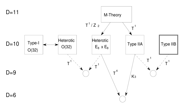
Figure 19: The web of duality symmetries between string theories. Broken lines correspond to perturbative duality connections. Type-IIB in ten dimensions is supposed to be self-dual under SL(2,ℤ).

In the type-II case the situation is similar. We compactify on a circle. Under an $R\to 1/R$ duality

$$\partial X^{9}\to\partial X^{9}\;\;\;,\;\;\;\psi^{9}\to\psi^{9}\;\;\;,\;\;\;\bar{\partial}X^{9}\to-\bar{\partial}X^{9}\;\;\;,\;\;\;\bar{\psi}^{9}\to-\bar{\psi}^{9}\,.$$ (14.5)

Due to the change of sign of $\bar{\psi}^{9}$ the projection in the $\bar{R}$ sector is reversed. Consequently the duality maps type-IIA to type-IIB and vice versa. We can also phrase this in the following manner: the $R\to\infty$ limit of the toroidally compactified type-IIA string gives the type-IIA theory in ten dimensions. The $R\to 0$ limit gives the type-IIB theory in ten dimensions.

Apart from these perturbative connections, today we have evidence that all supersymmetric string theories are connected. Since they look very different in perturbation theory, the connections necessarily involve strong coupling.

First, there is evidence that the type-IIB theory has an SL(2,ℤ) symmetry that, among other things, inverts the coupling constant [57]. Consequently, the strong coupling limit of type-IIB is isomorphic to the perturbative type-IIB theory. Upon compactification this symmetry combines with the perturbative $T$-duality symmetries to produce a large discrete duality group known as the $U$-duality group, which is the discretization of the non-compact continuous symmetries of the maximal effective supergravity theory. In table 3 below, the $U$-duality groups are given for various dimensions. They were conjectured to be exact symmetries in [58]. A similar remark applies to non-trivial compactifications.

Dimension SUGRA symmetry T-duality U-duality 10A SO(1,1,ℝ)/Z₂ 1 1 10B SL(2,ℝ) 1 SL(2,ℤ) 9 SL(2,ℝ)$\times$O(1,1,ℝ) Z₂ SL(2,ℤ)$\times$Z₂ 8 SL(3,ℝ)$\times$SL(2,ℝ) O(2,2,ℤ) SL(3,ℤ)$\times$SL(2,ℤ) 7 SL(5,ℝ) O(3,3,ℤ) SL(5,ℤ) 6 O(5,5,ℝ) O(4,4,ℤ) O(5,5,ℤ) 5 E₆₍₆₎ O(5,5,ℤ) E₆₍₆₎(ℤ) 4 E₇₍₇₎ O(6,6,ℤ) E₇₍₇₎(ℤ) 3 E₈₍₈₎ O(7,7,ℤ) E₈₍₈₎(ℤ)

Table 3: Duality symmetries for the compactified type-II string.

Also, it can be argued that the strong coupling limit of type-IIA theory is described by an eleven-dimensional theory named “M-theory” [59]. Its low-energy limit is eleven-dimensional supergravity. Compactification of M-theory on a circle of very small radius gives the perturbative type-IIA theory.

If instead we compactify M-theory on the $Z_{2}$ orbifold of the circle $T^{1}/Z_{2}$ then we obtain the heterotic E${}_{8}\times$E₈ theory [60]. When the circle is large the heterotic theory is strongly coupled, while for small radius it is weakly coupled.

Finally, the strong coupling limit of the O(32) heterotic string theory is the type-I O(32) theory and vice versa [61].

There is another non-trivial non-perturbative connection in six dimensions: the strong coupling limit of the six-dimensional toroidally compactified heterotic string is given by the type-IIA theory compactified on K3 and vice versa [58].

Thus, we are led to suspect that there is an underlying “universal” theory whose various limits in its “moduli” space produce the weakly coupled ten-dimensional supersymmetric string theories as depicted in Fig. 20 (borrowed from [10]). The correct description of this theory is unknown, although there is a proposal that it might have a matrix description [62], inspired from D-branes [63], which reproduces the perturbative IIA string in ten dimensions [64].

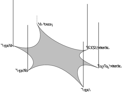
Figure 20: A unique theory and its various limits.

We will provide with a few more explanations and arguments supporting the non-perturbative connections mentioned above. But before we get there, we will need some “non-perturbative tools”, namely the notion of BPS states and p-branes, which I will briefly describe.

14.1 Antisymmetric tensors and p-branes

We have seen that the various string theories have massless antisymmetric tensors in their spectrum. We will use the language of forms and we will represent a rank-p antisymmetric tensor $A_{\mu_{1}\mu_{2}\ldots\mu_{p}}$ by the associated p-form

$$A_{p}\equiv A_{\mu_{1}\mu_{2}\ldots\mu_{p}}dx^{\mu_{1}}\wedge\ldots\wedge dx^{\mu_{p}}\,.$$ (14.1.1)

Such p-forms transform under generalized gauge transformations:

$$A_{p}\to A_{p}+d~{}\Lambda_{p-1},\,,$$ (14.1.2)

where $d$ is the exterior derivative ($d^{2}=0$) and $\Lambda_{p-1}$ is a $(p-1)$-form that serves as the parameter of gauge transformations. The familiar case of (abelian) gauge fields corresponds to p=1. The gauge-invariant field strength is

$$F_{p+1}=d~{}A_{p}\,.$$ (14.1.3)

satisfying the free Maxwell equations

$$d^{*}F_{p+1}=0$$ (14.1.4)

The natural objects, charged under a (p+1)-form $A_{p+1}$, are $p$-branes. A $p$-brane is an extended object with $p$ spatial dimensions. Point particles correspond to p=0, strings to p=1. The natural coupling of $A_{p+1}$ and a p-brane is given by

$$\exp\left[iQ_{p}\int_{\rm world-volume}A_{p+1}\right]=\exp\left[iQ_{p}\int A_{\mu_{0}\ldots\mu_{p}}dx^{\mu_{0}}\wedge\ldots\wedge dx^{\mu_{p}}\right]\,,$$ (14.1.5)

which generalizes the Wilson line coupling in the case of electromagnetism. The world-volume of $p$-brane is (p+1)-dimensional. Note also that this is precisely the $\sigma$-model coupling of the usual string to the $NS$ antisymmetric tensor in (9.1). The charge $Q_{p}$ is the usual electric charge for p=0 and the string tension for p=1. For the p-branes we will be considering, the (electric) charges will be related to their tensions (mass per unit volume).

In analogy with electromagnetism, we can also introduce magnetic charges. First, we must define the analog of the magnetic field: the magnetic (dual) form. This is done by first dualizing the field strength and then rewriting it as the exterior derivative of another form :

$$d\tilde{A}_{D-p-3}=\tilde{F}_{D-p-2}=^{*}F_{p+2}=^{*}dA_{p+1}\,,$$ (14.1.6)

where D is the the dimension of spacetime. Thus, the dual (magnetic) form couples to $(D-p-4)$-branes that play the role of magnetic monopoles with “magnetic charges” $\tilde{Q}_{D-p-4}$.

There is a generalization of the Dirac quantization condition to general p-form charges discovered by Nepomechie and Teitelboim [65]. The argument parallels that of Dirac. Consider an electric p-brane with charge $Q_{p}$ and a magnetic $(D-p-4)$-brane with charge $\tilde{Q}_{D-p-4}$. Normalize the forms so that the kinetic term is ${1\over 2}\int^{*}F_{p+2}F_{p+2}$. Integrating the field strength $F_{p+2}$ on a (D-p-2)-sphere surrounding the p-brane we obtain the total flux $\Phi=Q_{p}$. We can also write

$$\Phi=\int_{S^{D-p-2}}~{}^{*}F_{p+2}=\int_{S^{D-p-3}}~{}\tilde{A}_{D-p-3}\,,$$ (14.1.7)

where we have used (14.1.6) and we have integrated around the “Dirac string”. When the magnetic brane circles the Dirac string it picks up a phase $e^{i\Phi\tilde{Q}_{D-p-4}}$, as can be seen from (14.1.5). Unobservability of the string implies the Dirac-Nepomechie-Teitelboim quantization condition

$$\Phi\tilde{Q}_{D-p-4}=Q_{p}\tilde{Q}_{D-p-4}=2\pi N\;\;\;,\;\;\;n\in Z\,.$$ (14.1.8)

14.2 BPS states and bounds

The notion of BPS states is of capital importance in discussions of non-perturbative duality symmetries. Massive BPS states appear in theories with extended supersymmetry. It just so happens that supersymmetry representations are sometimes shorter than usual. This is due to some of the supersymmetry operators being “null”, so that they cannot create new states. The vanishing of some supercharges depends on the relation between the mass of a multiplet and some central charges appearing in the supersymmetry algebra. These central charges depend on electric and magnetic charges of the theory as well as on expectation values of scalars (moduli). In a sector with given charges, the BPS states are the lowest lying states and they saturate the so-called BPS bound which, for point-like states, is of the form

$$M\geq~{}{\rm maximal~{}~{}eigenvalue~{}~{}of}\;\;Z\,,$$ (14.2.1)

where $Z$ is the central charge matrix. This is shown in Appendix D where we discuss in detail the representations of extended supersymmetry in four dimensions.

BPS states behave in a very special way:

$\bullet$ At generic points in moduli space they are absolutely stable. The reason is the dependence of their mass on conserved charges. Charge and energy conservation prohibits their decay. Consider as an example, the BPS mass formula

$$M^{2}_{m,n}={|m+n\tau|^{2}\over\tau_{2}}\;\;,$$ (14.2.2)

where $m,n$ are integer-valued conserved charges, and $\tau$ is a complex modulus. This BPS formula is relevant for N=4, SU(2) gauge theory, in a subspace of its moduli space. Consider a BPS state with charges $(m_{0},n_{0})$, at rest, decaying into N states with charges $(m_{i},n_{i})$ and masses $M_{i}$, $i=1,2,\cdots,N$. Charge conservation implies that $m_{0}=\sum_{i=1}^{N}m_{i}$, $n_{0}=\sum_{i=1}^{N}n_{i}$. The four-momenta of the produced particles are $(\sqrt{M_{i}^{2}+\vec{p}_{i}^{2}},\vec{p}_{i})$ with $\sum_{i=1}^{N}\vec{p}_{i}=\vec{0}$. Conservation of energy implies

$$M_{m_{0},n_{0}}=\sum_{i=1}^{N}\sqrt{M_{i}^{2}+\vec{p}^{2}_{i}}\geq\sum_{i=1}^{N}M_{i}\;\;.$$ (14.2.3)

Also in a given charge sector (m,n) the BPS bound implies that any mass $M\geq M_{m,n}$, with $M_{m,n}$ given in (14.2.2). Thus, from (14.2.3) we obtain

$$M_{m_{0},n_{0}}\geq\sum_{i=1}^{N}M_{m_{i},n_{i}}\;\;,$$ (14.2.4)

and the equality will hold if all particles are BPS and are produced at rest ($\vec{p}_{i}=\vec{0}$). Consider now the two-dimensional vectors $v_{i}=m_{i}+\tau n_{i}$ on the complex $\tau$-plane, with length $||v_{i}||^{2}=|m_{i}+n_{i}\tau|^{2}$. They satisfy $v_{0}=\sum_{i=1}^{N}v_{i}$. Repeated application of the triangle inequality implies

$$||v_{0}||\leq\sum_{i=1}^{N}||v_{i}||\;\;.$$ (14.2.5)

This is incompatible with energy conservation (14.2.4) unless all vectors $v_{i}$ are parallel. This will happen only if $\tau$ is real. For energy conservation it should also be a rational number. On the other hand, due to the SL(2,ℤ) invariance of (14.2.2), the inequivalent choices for $\tau$ are in the SL(2,$\hbox{\mybb Z})$ fundamental domain and $\tau$ is never real there. In fact, real rational values of $\tau$ are mapped by SL(2,$\hbox{\mybb Z})$ to $\tau_{2}=\infty$, and since $\tau_{2}$ is the inverse of the coupling constant, this corresponds to the degenerate case of zero coupling. Consequently, for $\tau_{2}$ finite, in the fundamental domain, the BPS states of this theory are absolutely stable. This is always true in theories with more than eight conserved supercharges (corresponding to N$>2$ supersymmetry in four dimensions). In cases corresponding to theories with 8 supercharges, there are regions in the moduli space, where BPS states, stable at weak coupling, can decay at strong coupling. However, there is always a large region around weak coupling where they are stable.

$\bullet$ Their mass-formula is supposed to be exact if one uses renormalized values for the charges and moduli. The argument is that quantum corrections would spoil the relation of mass and charges, if we assume unbroken SUSY at the quantum level. This would give incompatibilities with the dimension of their representations. Of course this argument seems to have a loophole: a specific set of BPS multiplets can combine into a long one. In that case, the above argument does not prohibit corrections. Thus, we have to count BPS states modulo long supermultiplets. This is precisely what helicity supertrace formulae do for us. They are reviewed in detail in Appendix E. Even in the case of N=1 supersymmetry there is an analog of BPS states, namely the massless states.

There are several amplitudes that in perturbation theory obtain contributions from BPS states only. In the case of eight conserved supercharges (N=2 supersymmetry in four dimensions), all two-derivative terms as well as $R^{2}$ terms are of that kind. In the case of sixteen conserved supercharges (N=4 supersymmetry in four dimensions), except the above terms, also the four derivative terms as well as $R^{4}$, $R^{2}F^{2}$ terms are of a similar kind. The normalization argument of the BPS mass-formula makes another important assumption: as the coupling grows, there is no phase transition during which supersymmetry is (partially) broken.

The BPS states described above can be realized as point-like soliton solutions of the relevant effective supergravity theory. The BPS condition is the statement that the soliton solution leaves part of the supersymmetry unbroken. The unbroken generators do not change the solution, while the broken ones generate the supermultiplet of the soliton, which is thus shorter than the generic supermultiplet.

So far we discussed point-like BPS states. There are however BPS versions for extended objects (BPS p-branes). In the presence of extended objects the supersymmetry algebra can acquire central charges that are not Lorentz scalars (as we assumed in Appendix D). Their general form can be obtained from group theory, in which case one sees that they must be antisymmetric tensors, $Z_{\mu_{1}\ldots\mu_{p}}$. Such central charges have values proportional to the charges $Q_{p}$ of p-branes. Then, the BPS condition would relate these charges with the energy densities (p-brane tensions) $\mu_{p}$ of the relevant p-branes. Such p-branes can be viewed as extended soliton solutions of the effective theory. The BPS condition is the statement that the soliton solution leaves some of the supersymmetries unbroken.

14.3 Heterotic/type-I duality in ten dimensions.

We will start our discussion by describing heterotic/type-I duality in ten dimensions. It can be shown [66] that heterotic/type-I duality, along with T-duality can reproduce all known string dualities.

Consider first the O(32) heterotic string theory. At tree-level (sphere) and up to two-derivative terms, the (bosonic) effective action in the $\sigma$-model frame is

$$S^{\rm het}=\int d^{10}x\sqrt{G}e^{-\Phi}\left[R+(\nabla\Phi)^{2}-{1\over 12}\hat{H}^{2}-{1\over 4}F^{2}\right]\,.$$ (14.3.1)

On the other hand, for the O(32) type-I string the leading order two-derivative effective action is

$$S^{I}=\int d^{10}x\sqrt{G}\left[e^{-\Phi}\left(R+(\nabla\Phi)^{2}\right)-{1\over 4}e^{-\Phi/2}F^{2}-{1\over 12}\hat{H}^{2}\right]\,.$$ (14.3.2)

The different dilaton dependence here comes as follows: the Einstein and dilaton terms come from the closed sector on the sphere ($\chi=2$). The gauge kinetic terms come from the disk ($\chi=1$). Since the antisymmetric tensor comes from the $R$-$R$ sector of the closed superstring it does not have any dilaton dependence on the sphere.

We will now bring both actions to the Einstein frame, $G_{\mu\nu}=e^{\Phi/4}g_{\mu\nu}$:

$$S^{\rm het}_{E}=\int d^{10}x\sqrt{g}\left[R-{1\over 8}(\nabla\Phi)^{2}-{1\over 4}e^{-\Phi/4}F^{2}-{1\over 12}e^{-\Phi/2}\hat{H}^{2}\right]\,,$$ (14.3.3)

$$S^{I}_{E}=\int d^{10}x\sqrt{g}\left[R-{1\over 8}(\nabla\Phi)^{2}-{1\over 4}e^{\Phi/4}F^{2}-{1\over 12}e^{\Phi/2}\hat{H}^{2}\right]\,.$$ (14.3.4)

We observe that the two actions are related by $\Phi\to-\Phi$ while keeping the other fields invariant. This seems to suggest that the weak coupling of one is the strong coupling of the other and vice versa. Of course, the fact that the two actions are related by a field redefinition is not a surprise. It is known that N=1 ten-dimensional supergravity is completely fixed once the gauge group is chosen. It is interesting though, that the field redefinition here is just an inversion of the ten-dimensional coupling. Moreover, the two theories have perturbative expansions that are very different.

We would like to go further and check if there are non-trivial checks of what is suggested by the classical N=1 supergravity. However, once we compactify one direction on a circle of radius $R$ we seem to have a problem. In the heterotic case, we have a spectrum that depends both on momenta $m$ in the ninth direction as well as on windings $n$. The winding number is the charge that couples to the string antisymmetric tensor. In particular, it is the electric charge of the gauge boson obtained from $B_{9\mu}$. On the other hand, in type-I theory, as we have shown earlier, we have momenta $m$ but no windings. One way to see this is that the open string Neumann boundary conditions forbid the string to wind around the circle. Another way is by noting that the $NS$-$NS$ antisymmetric tensor that could couple to windings has been projected out by our orientifold projection.

However, we do have the $R$-$R$ antisymmetric tensor, but as we argued in section 10.2, no perturbative states are charged under it. There may be, however, non-perturbative states that are charged under this antisymmetric tensor. According to our general discussion in section 14.1 this antisymmetric tensor would naturally couple to a string, but this is certainly not the perturbative string. How can we construct this non-perturbative string?

An obvious guess is that this is a solitonic string excitation of the low-energy type-I effective action. Indeed, such a solitonic solution was constructed [68] and shown to have the correct zero mode structure.

We can give a more complete description of this non-perturbative string. The hint is given from $T$-duality on the heterotic side, which interchanges windings and momenta. When it acts on derivatives of $X$ it interchanges $\partial_{\sigma}X\leftrightarrow\partial_{\tau}X$. Consequently, Neumann boundary conditions are interchanged with Dirichlet ones. To construct such a non-perturbative string we would have to use also Dirichlet boundary conditions. Such boundary conditions imply that the open string boundary is fixed in spacetime. In terms of waves traveling on the string, it implies that a wave arriving at the boundary is reflected with a minus sign. The interpretation of fixing the open string boundary in some (submanifold) of spacetime has the following interpretation: there is a solitonic (extended) object there whose fluctuations are described by open strings attached to it. Such objects are known today as D-branes.

Thus, we would like to describe our non-perturbative string as a D1-brane. We will localize it to the hyperplane $X^{2}=X^{3}=\ldots=X^{9}=0$. Its world-sheet extends in the $X^{0},X^{1}$ directions. Such an object is schematically shown in Fig. 21. Its fluctuations can be described by two kinds of open strings:

Figure 21: Open string fluctuations of a D1-brane

$\bullet$ DD strings that have D-boundary conditions on both end-points and are forced to move on the D1-brane.

$\bullet$ DN strings that have a D-boundary condition on one end, which is stuck on the D1-brane, and N-boundary conditions on the other end, which is free.

As we will see, this solitonic configuration breaks half of N=2 spacetime supersymmetry possible in ten dimensions. It also breaks $SO(9,1)\to SO(8)\times SO(1,1)$. Moreover, we can put it anywhere in the transverse eight-dimensional space, so we expect eight bosonic zero-modes around it associated with the broken translational symmetry. We will try to understand in more detail the modes describing the world-sheet theory of the D1 string. We can obtain them by looking at the massless spectrum of the open string fluctuations around it.

Start with the DD strings. Here $X^{I},\psi^{I},\bar{\psi}^{I}$, $I=2,\ldots,9$ have DD boundary conditions while $X^{\mu},\psi^{\mu},\bar{\psi}^{\mu}$, $\mu=0,1$ have NN boundary conditions.

For the world-sheet fermions NN boundary conditions imply

$${\rm NN~{}~{}NS~{}~{}sector}~{}~{}~{}~{}~{}~{}~{}~{}~{}\left.\psi+\bar{\psi}\right|_{\sigma=0}=\left.\psi-\bar{\psi}\right|_{\sigma=\pi}=0\,,$$ (14.3.5)

$${\rm NN~{}~{}R~{}~{}sector}~{}~{}~{}~{}~{}~{}~{}~{}~{}\left.\psi-\bar{\psi}\right|_{\sigma=0}=\left.\psi-\bar{\psi}\right|_{\sigma=\pi}=0\,.$$ (14.3.6)

The DD boundary condition is essentially the same with $\bar{\psi}\to-\bar{\psi}$:

$${\rm DD~{}~{}NS~{}~{}sector}~{}~{}~{}~{}~{}~{}~{}~{}~{}\left.\psi-\bar{\psi}\right|_{\sigma=0}=\left.\psi+\bar{\psi}\right|_{\sigma=\pi}=0\,,$$ (14.3.7)

$${\rm DD~{}~{}R~{}~{}sector}~{}~{}~{}~{}~{}~{}~{}~{}~{}\left.\psi+\bar{\psi}\right|_{\sigma=0}=\left.\psi+\bar{\psi}\right|_{\sigma=\pi}=0\,,$$ (14.3.8)

and a certain action on the Ramond ground-state, which we will describe below.

Exercise Show that we have the following mode expansions

$$X^{I}(\sigma,\tau)=x^{I}+w^{I}\sigma+2\sum_{n\not=0}{a^{I}_{n}\over n}e^{in\tau}\sin(n\sigma)\,,$$ (14.3.9)

$$X^{\mu}(\sigma,\tau)=x^{\mu}+p^{\mu}\tau-2i\sum_{n\not=0}{a^{\mu}_{n}\over n}e^{in\tau}\cos(n\sigma)\,.$$ (14.3.10)

In the $NS$ sector

$$\psi^{I}(\sigma,\tau)=\sum_{n\in Z}b^{I}_{n+1/2}e^{i(n+1/2)(\sigma+\tau)}\;\;\;,\;\;\;\psi^{\mu}(\sigma,\tau)=\sum_{n\in Z}b^{\mu}_{n+1/2}e^{i(n+1/2)(\sigma+\tau)}\,,$$ (14.3.11)

while in the $R$ sector

$$\psi^{I}(\sigma,\tau)=\sum_{n\in Z}b^{I}_{n}e^{in(\sigma+\tau)}\;\;\;,\;\;\;\psi^{\mu}(\sigma,\tau)=\sum_{n\in Z}b^{\mu}_{n}e^{in(\sigma+\tau)}\,.$$ (14.3.12)

Also

$$\bar{b}^{I}_{n+1/2}=b^{I}_{n+1/2}\;\;\;,\;\;\;\bar{b}^{I}_{n}=-b^{I}_{n}\,,$$ (14.3.13)

$$\bar{b}^{\mu}_{n+1/2}=-b^{\mu}_{n+1/2}\;\;\;,\;\;\;\bar{b}^{\mu}_{n}=b^{\mu}_{n}\,.$$ (14.3.14)

The $x^{I}$ in (14.3.9) are the position of the D-string in transverse space. There is no momentum in (14.3.9), which implies that the state wavefunctions would depend only on the $X^{0,1}$ coordinates, since there is a continuous momentum in (14.3.10). Thus, the states of this theory “live” on the world-sheet of the D1-string. The usual bosonic massless spectrum would consist of a vector $A_{\mu}(x^{0},x^{1})$ corresponding to the state $\psi^{\mu}_{-1/2}|0\rangle$ and eight bosons $\phi^{I}(x^{0},X^{1})$ corresponding to the states $\psi^{I}_{-1/2}|0\rangle$. We will now consider the action of the orientation reversal $\Omega$: $\sigma\to-\sigma$, $\psi\leftrightarrow\bar{\psi}$. Using (14.3.5)-(14.3.8),

$$\Omega~{}b^{\mu}_{-1/2}|0\rangle=\bar{b}^{\mu}_{-1/2}|0\rangle=-b^{\mu}_{-1/2}|0\rangle\,,$$ (14.3.15)

$$\Omega~{}b^{I}_{-1/2}|0\rangle=\bar{b}^{I}_{-1/2}|0\rangle=b^{I}_{-1/2}|0\rangle\,.$$ (14.3.16)

The vector is projected out, while the eight bosons survive the projection.

We will now analyze the Ramond sector, where fermionic degrees of freedom would come from. The massless ground-state $|R\rangle$ is an SO(9,1) spinor satisfying the usual GSO projection

$$\Gamma^{11}|R\rangle=|R\rangle\,.$$ (14.3.17)

Consider now the $\Omega$ projection on that spinor. In the usual $NN$ case $\Omega$ can be taken to commute with $(-1)^{F}$ and acts on the spinor ground-state as $-1$. In the DD case the action of $\Omega$ on the transverse DD fermionic coordinates is reversed compared to the NN case. On the spinor this action is

$$\Omega|R\rangle=-\Gamma^{2}\ldots\Gamma^{9}|R\rangle=|R\rangle\,.$$ (14.3.18)

From (14.3.17), (14.3.18) we also obtain

$$\Gamma^{0}\Gamma^{1}|R\rangle=-|R\rangle\,.$$ (14.3.19)

If we decompose the spinor under SO(8)$\times$SO(1,1) the surviving piece transforms as $8_{-}$ where $-$ refers to the SO(1,1) chirality (14.3.19). As for the bosons, these fermions are functions of $X^{0,1}$ only.

To recapitulate, in the DD sector we have found the following massless fluctuations moving on the world-sheet of the D1-string: 8 bosons and 8 chirality minus fermions.

Consider now the DN fluctuations. In this case Chan-Paton factors are allowed in the free string end, and the usual tadpole cancelation argument implies that there are 32 of them. In this case, the boundary conditions for the transverse bosons and fermions become

$$\left.\partial_{\tau}X^{I}\right|_{\sigma=0}=0\;\;\;,\;\;\;\left.\partial_{\sigma}X^{I}\right|_{\sigma=\pi}=0\,,$$ (14.3.20)

$${\rm DN~{}~{}NS~{}~{}sector}~{}~{}~{}~{}~{}~{}~{}~{}~{}\left.\psi+\bar{\psi}\right|_{\sigma=0}=\left.\psi+\bar{\psi}\right|_{\sigma=\pi}=0\,,$$ (14.3.21)

$${\rm DN~{}~{}R~{}~{}sector}~{}~{}~{}~{}~{}~{}~{}~{}~{}\left.\psi-\bar{\psi}\right|_{\sigma=0}=\left.\psi+\bar{\psi}\right|_{\sigma=\pi}=0\,,$$ (14.3.22)

while they are NN in the longitudinal directions.

We observe that here, the bosonic oscillators are half-integrally modded as in the twisted sector of $Z_{2}$ orbifolds. Thus, the ground-state conformal weight is 8/16=1/2. Also the modding for the fermions has been reversed between the $NS$ and $R$ sectors. In the $NS$ sector the fermionic ground-state is also a spinor with ground-state conformal weight 1/2. The total ground-state has conformal weight 1 and only massive excitations are obtained in this sector.

In the $R$ sector there are massless states coming from the bosonic ground-state combined with the O(1,1) spinor ground-state from the longitudinal Ramond fermions. The usual GSO projection here is $\Gamma^{0}\Gamma^{1}=1$. Thus, the massless modes in the DN sector are 32 chirality plus fermions.

In total, the world-sheet theory of the D-string contains exactly what we would expect from the heterotic string in the physical gauge! This is a non-trivial argument in favor of heterotic/type-I duality.

Exercise. We have considered so far a D1-brane in type-I theory. Consider the general case of Dp-branes along similar lines. Show that non-trivial configurations exist (compatible with GSO and $\Omega$ projections) preserving half of the supersymmetry, for p=1,5,9. The case p=9 corresponds to the usual open strings moving in 10-d space.

The $R$-$R$ two-form couples to a one-brane (electric) and a five-brane (magnetic). As we saw above, both can be constructed as D-branes.

We will describe now in some more detail the D5-brane, since it involves some novel features. To construct a five-brane, we will have to impose Dirichlet boundary conditions in four transverse directions. We will again have DD and NN sectors, as in the D1 case. The massless fluctuations will have continuous momentum in the six longitudinal directions, and will describe fields living on the six-dimensional world-volume of the five-brane. Since we are breaking half of the original supersymmetry, we expect that the world-volume theory will have N=1 six-dimensional supersymmetry, and the massless fluctuations will form multiplets of this supersymmetry. The relevant multiplets are the vector multiplet, containing a vector and a gaugino, as well as the hypermultiplet, containing four real scalars and a fermion. Supersymmetry implies that the manifold of the hypermultiplet scalars is a hyper-Kähler manifold. When the hypermultiplets are charged under the gauge group, the gauge transformations are isometries of the hyper-Kähler manifold, of a special type: they are compatible with the hyper-Kähler structure.

It will be important for our latter purposes to describe the Higgs effect in this case. When a gauge theory is in the Higgs phase, the gauge bosons become massive by combining with some of the massless Higgs modes. The low-energy theory (for energies well below the gauge boson mass) is described by the scalars that have not been devoured by the gauge bosons. In our case, each (six-dimensional) gauge boson that becomes massive, will eat-up four scalars (a hypermultiplet). The left over low-energy theory of the scalars will be described by a smaller hyper-Kähler manifold (since supersymmetry is not broken during the Higgs phase transition). This manifold is constructed by a mathematical procedure known as the hyper-Kähler quotient. The procedure “factors out” the isometries of a hyper-Kähler manifold to produce a lower-dimensional manifold which is still hyper-Kähler. Thus, the hyper-Kähler quotient construction is describing the ordinary Higgs effect in six-dimensional N=1 gauge theory.

The D5-brane we are about to construct is mapped via heterotic/type-I duality to the NS5-brane of the heterotic theory. The NS5-brane has been constructed [49] as a soliton of the effective low-energy heterotic action. The non-trivial fields, in the transverse space, are essentially configurations of axion-dilaton instantons, together with four-dimensional instantons embedded in the O(32) gauge group. Such instantons have a size that determines the “thickness” of the NS5-brane. The massless fluctuations are essentially the moduli of the instantons. There is a mathematical construction of this moduli space, as a hyper-Kähler quotient. This leads us to suspect [67] that the interpretation of this construction is a Higgs effect in the six-dimensional world-volume theory. In particular, the mathematical construction implies that for N coincident NS5-branes, the hyper-Kähler quotient construction implies that an Sp(N) gauge group is completely Higgsed. For a single five-brane, the gauge group is $\rm Sp(1)\sim SU(2)$. Indeed, if the size of the instanton is not zero, the massless fluctuations of the NS5-brane form hypermultiplets only. When the size becomes zero, the moduli space has a singularity, which can be interpreted as the restoration of the gauge symmetry: at this point the gauge bosons become massless again. All of this indicates that the world-volume theory of a single five-brane should contain an SU(2) gauge group, while in the case of N five-branes the gauge group is enhanced to Sp(N), [67].

We will now return to our description of the massless fluctuations of the D5-brane. The situation parallels the D1 case that we have described in detail. In particular, from the DN sectors we will obtain hypermultiplets only. From the DD sector we can in principle obtain massless vectors. However, as we have seen above, the unique vector that can appear is projected out by the orientifold projection. To remedy this situation we are forced to introduce a Chan-Paton factor for the Dirichlet end-points of the open string fluctuations. For a single D5-brane, this factor takes two values, $i=1,2$. Thus, the massless bosonic states in the DD sector are of the form

$$b_{-1/2}^{\mu}|p;i,j\rangle\;\;\;\;\;\;,\;\;\;\;\;\;b_{-1/2}^{I}|p;i,j\rangle\;.$$ (14.3.23)

We have also seen that the orientifold projection $\Omega$ changes the sign of $b_{-1/2}^{\mu}$ and leaves $b_{-1/2}^{I}$ invariant. The action of $\Omega$ on the ground-state is $\Omega|p;i,j\rangle=\epsilon|p;j,i\rangle$. It interchanges the Chan-Paton factors and can have a sign $\epsilon=\pm 1$. The number of vectors that survive the $\Omega$ projection depends on this sign. For $\epsilon=1$, only one vector survives and the gauge group is O(2). If $\epsilon=-1$, three vectors survive and the gauge group is $\rm Sp(1)\sim SU(2)$. Taking into account our previous discussion, we must take $\epsilon=-1$. Thus, we have an Sp(1) vector multiplet. The scalar states on the other hand will be forced to be antisymmetrized in the Chan-Paton indices. This will provide a single hypermultiplet, whose four scalars describe the position of the D5-brane in the four-dimensional transverse space. Finally, the DN sector has an $i=1,2$ Chan-Paton factor on the D-end and an $\alpha=1,2,\cdots,32$ factor on the Neumann end-point. Consequently, we will obtain a hypermultiplet transforming as $\bf(2,32)$ under $\rm Sp(1)\times O(32)$ where Sp(1) is the world-volume gauge group and O(32) is the original (spacetime) gauge group of the type-I theory.

In order to describe N parallel coinciding D5-branes, the only difference is that the Dirichlet Chan-Paton factor now takes 2N values. Going through the same procedure as above we find in the DD sector, Sp(N) vector multiplets, and hypermultiplets transforming as a singlet (the center-of-mass position coordinates) as well as the traceless symmetric tensor representation of Sp(N) of dimension $2N^{2}-N-1$. In the DN sector we find a hypermultiplet transforming as $\bf(2N,32)$ under $\rm Sp(N)\times O(32)$.

Exercise: Consider N parallel coincident D1-branes in the type-I theory. Show that the massless excitations are a two-dimensional vector in the adjoint representation of SO(N), eight scalars in the symmetric representation of SO(N), eight left-moving fermions in the adjoint of SO(N) and right-moving fermions transforming as $({\bf N,32})$ of SO(N)$\times$SO(32). This is in agreement with matrix theory compactified on $S^{1}/Z_{2}$ [72].

There are further checks of heterotic/type-I duality in ten dimensions. BPS-saturated terms in the effective action match appropriately between the two theories [69]. You can find a more detailed exposition of similar matters in [10].

The comparison becomes more involved and non-trivial upon toroidal compactification. First, the spectrum of BPS states is richer and different in perturbation theory in the two theories. Secondly, by adjusting moduli both theories can be compared in the weak coupling limit. The terms in the effective action that can be most easily compared are the $F^{4}$, $F^{2}R^{2}$ and $R^{4}$ terms. These are BPS-saturated and anomaly-related. In the heterotic string, they obtain perturbative corrections at one loop only. Also, their non-perturbative corrections are due to instantons that preserve half of the supersymmetry. Corrections due to generic instantons, that break more than 1/2 supersymmetry, vanish because of zero modes. In the heterotic string the only relevant non-perturbative configuration is the NS5-brane. Taking its world-volume to be Euclidean and wrapping it supersymmetrically around a compact manifold (so that the classical action is finite), it provides the relevant instanton configurations. Since we need at least a six-dimensional compact manifold to wrap it, we can immediately deduce that the BPS-saturated terms do not have non-perturbative corrections for toroidal compactifications with more than four non-compact directions. Thus, for $D>4$ the full heterotic result is tree-level and one-loop.

In the type-I string the situation is slightly different. Here we have both the D1-brane and the D5-brane that can provide instanton configurations. Again, the D5-brane will contribute in four dimensions. However, the D1-brane has a two-dimensional world-sheet and can contribute already in eight dimensions. We conclude that, in nine dimensions, the two theories can be compared in perturbation theory. This has been done [70]. They do agree at one loop. On the type-I side, however, duality also implies contact contributions for the factorizable terms $({\rm tr}R^{2})^{2}$, tr$F^{2}{\rm tr}R^{2}$ and $({\rm tr}F^{2})^{2}$ coming from surfaces with Euler number $\chi=-1,-2$.

In eight dimensions, the perturbative heterotic result is mapped via duality to perturbative as well as non-perturbative type-I contributions coming from the D1-instanton. These have been computed and duality has been verified [71].

14.4 Type-IIA versus M-theory.

We have mentioned in section 10.6, that the effective type-IIA supergravity is the dimensional reduction of eleven-dimensional, N=1 supergravity. We will see here that this is not just an accident [58, 59].

We will first review the spectrum of forms in type-IIA theory in ten dimensions.

$\bullet$ $NS$-$NS$ two-form B. Couples to a string (electrically) and a five-brane (magnetically). The string is the perturbative type-IIA string.

$\bullet$ $R$-$R$ U(1) gauge field A_μ. Can couple electrically to particles (zero-branes) and magnetically to six-branes. Since it comes from the $R$-$R$ sector no perturbative state is charged under it.

$\bullet$ $R$-$R$ three-form C_μνρ. Can couple electrically to membranes (p=2) and magnetically to four-branes.

$\bullet$ There is also the non-propagating zero-form field strength and ten-form field strength that would couple to eight-branes (see section 10.2).

As stated in section 10.6, the lowest-order type-IIA Lagrangian is

$$\tilde{S}^{IIA}={1\over 2\kappa^{2}_{10}}\left[\int d^{10}x\sqrt{g}e^{-\Phi}\left[\left(R+(\nabla\Phi)^{2}-{1\over 12}H^{2}\right)-{1\over 2\cdot 4!}\hat{G}^{2}-{1\over 4}F^{2}\right]+\right.$$

$$+\left.{1\over(48)^{2}}\int B\wedge G\wedge G\right].$$ (14.4.1)

We are in the string frame. Note that the $R$-$R$ kinetic terms do not couple to the dilaton as already argued in section 10.2.

In the type-IIA supersymmetry algebra there is a central charge proportional to the U(1) charge of the gauge field A:

$$\{Q^{1}_{\alpha},Q^{2}_{\dot{\alpha}}\}=\delta_{\alpha\dot{\alpha}}W\,.$$ (14.4.2)

This can be understood, since this supersymmetry algebra is coming from D=11 where instead of $W$ there is the momentum operator of the eleventh dimension. Since the U(1) gauge field is the $G_{11,\mu}$ component of the metric, the momentum operator becomes the U(1) charge in the type-IIA theory. There is an associated BPS bound

$$M\geq{c_{0}\over\lambda}|W|\,,$$ (14.4.3)

where $\lambda=e^{\Phi/2}$ is the ten-dimensional string coupling and $c_{0}$ some constant. States that satisfy this equality are BPS-saturated and form smaller supermultiplets. As mentioned above all perturbative string states have $W=0$. However, there is a soliton solution (black hole) of type-IIA supergravity with the required properties. In fact, the BPS saturation implies that it is an extremal black hole. We would expect that quantization of this solution would provide a (non-perturbative) particle state. Moreover, it is reasonable to expect that the U(1) charge is quantized in some units. Then the spectrum of these BPS states looks like

$$M={c\over\lambda}|n|\;\;\;,\;\;\;n\in Z\,.$$ (14.4.4)

At weak coupling these states are very heavy (but not as heavy as standard solitons whose masses scale with the coupling as $1/\lambda^{2}$). However, being BPS states, their mass can be reliably followed at strong coupling, where they become light, piling up at zero mass as the coupling becomes infinite. This is precisely the behavior of Kaluza-Klein (momentum) modes as a function of the radius. Since also the effective type-IIA field theory is a dimensional reduction of the eleven-dimensional supergravity, with $G_{11,11}$ becoming the string coupling, we can take this seriously [59] and claim that as $\lambda\to\infty$ type-IIA theory becomes some eleven-dimensional theory whose low-energy limit is eleven-dimensional supergravity. We can calculate the relation between the radius of the eleventh dimension and the string coupling. This was done essentially in section 10.6, where we described the dimensional reduction of eleven-dimensional N=1 supergravity to ten dimensions. The radius of the eleventh dimension $R$ can be obtained from (10.6.14) to be $R=e^{\sigma}$. The ten-dimensional type-IIA dilaton was found there to be $\Phi=3\sigma$. Thus,

$$R=\lambda^{2/3}\,.$$ (14.4.5)

At strong type-IIA coupling, $R\to\infty$ and the theory decompactifies to eleven dimensions, while in the perturbative regime the radius is small.

The eleven-dimensional theory (which has been named M-theory) contains the three-form that can couple to a membrane and a five-brane. Upon toroidal compactification to ten dimensions, the membrane, wrapped around the circle, becomes the perturbative type-IIA string that couples to $B_{\mu\nu}$. When it is not winding around the circle, then it is the type-IIA membrane coupling to the type-IIA three-form. The M-theory five-brane descends to the type-IIA five-brane or, wound around the circle, to the type-IIA four-brane.

14.5 M-theory and the E${}_{8}\times$E₈ heterotic string

M-theory has $Z_{2}$ symmetry under which the three-form changes sign. We might consider an orbifold of M-theory compactified on a circle of radius R, where the orbifolding symmetry is $x^{11}\to-x^{11}$ as well as the $Z_{2}$ symmetry mentioned above [60].

The untwisted sector can be obtained by keeping the fields invariant under the projection. It is not difficult to see that the ten-dimensional metric and dilaton survive the projection, while the gauge boson is projected out. Also the three-form is projected out, while the two-form survives. Half of the fermions survive, a Majorana-Weyl gravitino and a Mayorana-Weyl fermion of opposite chirality. Thus, in the massless spectrum, we are left with the N=1 supergravity multiplet. We do know by now that this theory is anomalous in ten dimensions. We must have some “twisted sector” that should arrange itself to cancel the anomalies. As we discussed in the section on orbifolds, $S^{1}/Z_{2}$ is a line segment, with the fixed-points $0,\pi$ at the boundary. The fixed-planes are two copies of ten-dimensional flat space. States coming from the twisted sector must be localized on these planes. We also have a symmetry exchanging the fixed planes, so we expect isomorphic massless content coming from the two fixed planes. It can also be shown that half of the anomalous variation is localized at one fixed plane and the other half at the other. The only N=1 multiplets that can cancel the anomaly symmetrically are vector multiplets, and we must have 248 of them at each fixed plane. The possible anomaly-free groups satisfying this constraint are $\rm E_{8}\times E_{8}$ and U(1)⁴⁹⁶. Since there is no known string theory associated with the second possibility, it is natural to assume that we have obtained the E${}_{8}\times$E₈ heterotic string theory. A similar argument to that of the previous section shows that there is a relation similar to (14.4.5) between the radius of the orbifold and the heterotic coupling. In the perturbative heterotic string, the two ten-dimensional planes are on top of each other and they move further apart as the coupling grows.

The M-theory membrane survives in the orbifold only if one of its dimensions is wound around the $S^{1}/Z_{2}$. It provides the perturbative heterotic string. On the other hand, the five-brane survives, and it cannot wind around the orbifold direction. It provides the heterotic NS5-brane. This is in accord with what we would expect from the heterotic string. Upon compactification to four dimensions, the NS5-brane will give rise to magnetically charged point-like states (monopoles).

14.6 Self-duality of the type-IIB string

In section 10.6 we have seen that the low-energy effective action of the type-IIB theory in ten dimensions has an SL(2,$\hbox{\mybb R})$ global symmetry. Its SL(2,ℤ) subgroup was conjectured [57, 58] to be an exact non-perturbative symmetry.

As described in section 10.2, the type-IIB theory in ten dimensions contains the following forms:

$\bullet$ The $NS$-$NS$ two-form $B^{1}$. It couples electrically to the perturbative type-IIB string (which we will call for later convenience the (1,0) string) and magnetically to a five-brane.

$\bullet$ The $R$-$R$ scalar. It is a zero-form (there is a Peccei-Quinn symmetry associated with it) and couples electrically to a ($-1$)-brane. Strictly speaking this is an instanton whose “world-volume” is a point in spacetime. It also couples magnetically to a seven-brane.

$\bullet$ The $R$-$R$ two-form $B^{2}$. It couples electrically to a (0,1) string (distinct from the perturbative type-II string) and magnetically to another (0,1) five-brane.

$\bullet$ The self-dual four-form. It couples to a self-dual three-brane.

As we have mentioned before, the low-energy effective theory is invariant under a continuous SL(2,$\hbox{\mybb R})$ symmetry, which acts by fractional transformations on the complex scalar $S$ defined in (10.6.20) and linearly on the vector of two-forms $(B^{1},B^{2})$, the four-form being invariant. The part of SL(2,ℝ) that translates the scalar is a symmetry of the full perturbative theory.

There is a (charge-one) BPS instanton solution in type-IIB theory given by the following configuration [73]

$$e^{\phi/2}=\lambda+{c\over r^{8}}\;\;\;,\;\;\;\chi=\chi_{0}+i{c\over\lambda(\lambda r^{8}+c)}\,,$$ (14.6.1)

where $r=|x-x_{0}|$, $x_{0}^{\mu}$ being the position of the instanton, $\lambda$ is the string coupling far away from the instanton, $c=\pi\sqrt{\pi}$ is fixed by the requirement that the solution has minimal instanton number and the other expectation values are trivial.

There is also a fundamental string solution, which is charged under $B^{1}$ (the (1,0) string) found in [74]. It has a singularity at the core, which is interpreted as a source for the fundamental type-IIB string. Acting with $S\to-1/S$ transformation on this solution we obtain [57] a solitonic string solution (the (0,1) string) that is charged under the $R$-$R$ antisymmetric tensor $B^{2}$. It is given by the following configuration [57]:

$$ds^{2}=A(r)^{-3/4}[-(dx^{0})^{2}+(dx^{1})^{2}]+A(r)^{1/4}dy\cdot dy\,,$$ (14.6.2)

$$S=\chi_{0}+i{e^{-\phi_{0}/2}\over\sqrt{A(r)}}\,,$$ (14.6.3)

$$B^{1}=0\;\;\;,\;\;\;B^{2}_{01}={1\over\sqrt{\Delta}A(r)}\,,$$ (14.6.4)

where

$$A(r)=1+{Q\sqrt{\Delta}\over 3r^{6}}\;\;\;,\;\;\;Q={3\kappa^{2}T\over\pi^{4}}\;\;\;,\;\;\;\Delta=e^{\phi_{0}/2}\left[\chi_{0}^{2}+e^{-\phi_{0}}\right]\,.$$ (14.6.5)

Here, $\kappa$ is Newton’s constant and $T=1/(2\pi\alpha^{\prime})$ is the tension of the perturbative type-IIB string. The tension of the (0,1) string can be calculated to be

$$\tilde{T}=T\sqrt{\Delta}\,.$$ (14.6.6)

In the perturbative regime, $e^{\phi_{0}}\to 0$, $\tilde{T}\sim Te^{-\phi_{0}/4}$ is large, and the (0,1) string is very stiff. Its vibrating modes cannot be seen in perturbation theory. However, at strong coupling, its fluctuations become the relevant low-energy modes. Acting further by SL(2,$\hbox{\mybb Z})$ transformations we can generate a multiplet of (p,q) strings with p,q relatively prime. If such solitons are added to the perturbative theory, the continuous SL(2,ℝ) symmetry is broken to SL(2,ℤ). All the (p,q) strings have a common massless spectrum given by the type-IIB supergravity content. Their massive excitations are distinct. Their string tension is given by

$$T_{p,q}=T{|p+qS|\over\sqrt{S_{2}}}\;\;.$$ (14.6.7)

By compactifying the type-IIB theory on a circle of radius $R_{B}$, it becomes equivalent to the IIA theory compactified on a circle. On the other hand, the nine-dimensional type-IIA theory is M-theory compactified on a two-torus.

From the type-IIB point of view, wrapping (p,q) strings around the tenth dimension provides a spectrum of particles in nine dimensions with masses

$$M^{2}_{B}={m^{2}\over R_{B}^{2}}+(2\pi R_{B}nT_{p,q})^{2}+4\pi T_{p,q}(N_{L}+N_{R})\;\;,$$ (14.6.8)

where $m$ is the Kaluza-Klein momentum integer, $n$ the winding number and $N_{L,R}$ the string oscillator numbers. The matching condition is $N_{L}-N_{R}=mn$, and BPS states are obtained for $N_{L}=0$ or $N_{R}=0$. We thus obtain the following BPS spectrum

$$\left.M^{2}_{B}\right|_{\rm BPS}=\left({m\over R_{B}}+2\pi R_{B}nT_{p,q}\right)^{2}\;\;.$$ (14.6.9)

Since an arbitrary pair of integers $(n_{1},n_{2})$ can be written as $n(p,q)$, where $n$ is the greatest common divisor and $p,q$ are relatively prime, we can rewrite the BPS mass formula above as

$$\left.M^{2}_{B}\right|_{BPS}=\left({m\over R_{B}}+2\pi R_{B}T{|n_{1}+n_{2}S|\over\sqrt{S_{2}}}\right)^{2}\;\;.$$ (14.6.10)

In M-theory, compactified on a two-torus with area $A_{11}$ and modulus $\tau$, we have two types of (point-like) BPS states in nine dimensions: KK states with mass $(2\pi)^{2}|n_{1}+n_{2}\tau|^{2}/(\tau_{2}A_{11})$ as well as states that are obtained by wrapping the M-theory membrane $m$ times around the two-torus, with mass $(mA_{11}T_{11})^{2}$, where $T_{11}$ is the tension of the membrane. We can also write $R_{11}$ that becomes the IIA coupling as $R_{11}^{2}=A_{11}/(4\pi^{2}\tau_{2})$. Thus, the BPS spectrum is

$$M_{11}^{2}=(m(2\pi R_{11})^{2}\tau_{2}T_{11})^{2}+{|n_{1}+n_{2}\tau|^{2}\over R_{11}^{2}\tau_{2}^{2}}+\cdots\;\;\;,$$ (14.6.11)

where the dots are mixing terms that we cannot calculate. The two BPS mass spectra should be related by $M_{11}^{2}=\beta M_{B}^{2}$, where $\beta\not=1$ since the masses are measured in different units in the two theories. Comparing, we obtain

$$S=\tau\;\;\;,\;\;\;{1\over R_{B}^{2}}=TT_{11}A_{11}^{3/2}\;\;\;,\;\;\;\beta=2\pi R_{11}{\sqrt{\tau_{2}}T_{11}\over T}\;\;.$$ (14.6.12)

An outcome of this is the calculation of the M-theory membrane tension $T_{11}$ in terms of string data.

There are several more tests of the consistency of assuming the SL(2,$\hbox{\mybb Z})$ symmetry in the IIB string, upon compactification. These include instanton calculations in ten or lower dimensions [75] as well as the existence of the “F-theory” structure [76] describing non-perturbative vacua of the IIB string.

14.7 D-branes are the type-II $R$-$R$ charged states

We have seen in section 14.3 that D-branes defined by imposing Dirichlet boundary conditions on some of the string coordinates provided non-perturbative extended solitons required by heterotic/type-I string duality.

Similar D-branes can also be constructed in type-II string theory, the only difference being that, here, there is no orientifold projection. Also, open string fluctuations around them cannot have Neumann (free) end-points. As we will see, such D-branes will provide all $R$-$R$ charged states required by the non-perturbative dualities of type-II string theory.

In the type-IIA theory we have seen that there are (in principle) allowed $R$-$R$ charged p-branes, with p$=0,2,4,6,8$, while in the type-IIB p$=-1,1,3,5,7$. D-branes can be constructed with a number of coordinates having D-boundary conditions being $9-$p$=1,2,\ldots,10$, which precisely matches the full allowed p-brane spectrum of type-II theories. The important question is: Are such D-branes charged under $R$-$R$ forms?

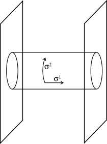
Figure 22: D-branes interacting via the tree-level exchange of a closed string.

To answer this question, we will have to study the tree-level interaction of two parallel Dp-branes via the exchange of a closed string [63], depicted schematically in Fig. 22. For this interpretation time runs horizontally. However, if we take time to run vertically, then, the same diagram can be interpreted as a (one-loop) vacuum fluctuation of open strings with their end-points attached to the D-branes. In this second picture we can calculate this diagram to be

$${\cal A}=2V_{p+1}\int{d^{p+1}k\over(2\pi)^{p+1}}\int_{0}^{\infty}{dt\over 2t}e^{-2\pi\alpha^{\prime}tk^{2}-t{|Y|^{2}\over 2\pi\alpha^{\prime}}}{1\over\eta^{12}(it)}{1\over 2}\sum_{a,b}(-1)^{a+b+ab}\vartheta^{4}[^{a}_{b}](it)$$ (14.7.1)

$$=2V_{p+1}\int_{0}^{\infty}{dt\over 2t}(8\pi^{2}\alpha^{\prime}t)^{-{p+1\over 2}}e^{-t{|Y|^{2}\over 2\pi\alpha^{\prime}}}{1\over\eta^{12}(it)}{1\over 2}\sum_{a,b=0}^{1}(-1)^{a+b+ab}\vartheta^{4}[^{a}_{b}](it)\,.$$

$V_{p+1}$ is the world-volume of the p-brane, the factor of 2 is due to the two end-points, $|Y|^{2}$ is the distance between the D-branes. Of course the total result is zero, because of the $\vartheta$-identity (A.15). This reflects the fact that the D-branes are BPS states and exert no static force on each other. However, our purpose is to disentangle the contributions of the various intermediate massless states in the closed string channel. This can be obtained by taking the leading $t\to 0$ behavior of the integrand. In order to do this, we have to perform a modular transformation $t\to 1/t$ in the $\vartheta$- and $\eta$-functions. We obtain

$$\left.{\cal A}\right|^{\rm closed~{}~{}string}_{\rm massless}=8(1-1)V_{p+1}\int_{0}^{\infty}{dt\over t}(8\pi^{2}\alpha^{\prime}t)^{-{p+1\over 2}}~{}t^{4}~{}e^{-{t|Y|^{2}\over 2\pi\alpha^{\prime}}}$$ (14.7.2)

$$=2\pi(1-1)V_{p+1}(4\pi^{2}\alpha^{\prime})^{3-p}G_{9-p}(|Y|)\;,$$

where

$$G_{d}(|Y|)={1\over 4\pi^{d/2}}\int_{0}^{\infty}{dt\over t^{(4-d)/2}}e^{-t|Y|^{2}}$$ (14.7.3)

is the massless scalar propagator in d dimensions. The $(1-1)$ comes from the $NS$-$NS$ and $R$-$R$ sectors respectively. Now consider the $R$-$R$ forms coupled to p-branes with action

$$S={\alpha_{p}\over 2}\int F_{p+2}\;^{*}F_{p+2}+iT_{p}\int_{\rm branes}A_{p+1}\,,$$ (14.7.4)

with $F_{p+2}=dA_{p+1}$. Using this action, the same amplitude for an exchange of $A_{p+1}$ between two D-branes at distance $|Y|$ in the transverse space of dimension $10-(p+1)=9-p$ is given by

$$\left.{\cal A}\right|_{\rm field~{}~{}theory}={(iT_{p})^{2}\over\alpha_{p}}V_{p+1}G_{9-p}(|Y|)\,,$$ (14.7.5)

where the factor of volume is present since the $R$-$R$ field can be absorbed or emitted at any point in the world-volume of the D-brane. Matching with the string calculation we obtain

$${T^{2}_{p}\over\alpha_{p}}=2\pi(4\pi^{2}\alpha^{\prime})^{3-p}\,.$$ (14.7.6)

We will now look at the DNT quantization condition which, with our normalization of the $R$-$R$ forms and $D=10$, becomes

$${T_{p}T_{6-p}\over\alpha_{p}}=2\pi n\,.$$ (14.7.7)

From (14.7.6) we can verify directly that D-branes satisfy this quantization condition for the minimum quantum $n=1$!

Thus, we are led to accept that D-branes, with a nice (open) CFT description of their fluctuations, describe non-perturbative extended BPS states of the type-II string carrying non-trivial $R$-$R$ charge.

We will now describe a uniform normalization of the D-brane tensions. Our starting point is the type-IIA ten-dimensional effective action (14.4.1). The gravitational coupling $\kappa_{10}$ is given in terms of $\alpha^{\prime}$ as

$$2\kappa_{10}^{2}=(2\pi)^{7}\alpha^{\prime 4}\;\;.$$ (14.7.8)

We will also normalize all forms so that their kinetic terms are $(1/4\kappa_{10}^{2})$ $\int d^{10}xF\otimes\tilde{F}$. This corresponds to $\alpha_{p}=1/(2\kappa_{10}^{2})$. We will also define the tensions of various p-branes via their world-volume action of the form

$$S_{p}=-T_{p}\int_{W_{p+1}}d^{p+1}\xi~{}e^{-\Phi/2}\sqrt{{\rm det}\hat{G}}-iT_{p}\int{}~{}A_{p+1}\;\;\;,$$ (14.7.9)

where $\hat{G}$ is the metric induced on the world-volume

$$\hat{G}_{\alpha\beta}=G_{\mu\nu}{\partial X^{\mu}\over\partial\xi^{\alpha}}{\partial X^{\nu}\over\partial\xi^{\beta}}$$ (14.7.10)

and

$$\int A_{p+1}={1\over(p+1)!}\int d^{p+1}\xi{}~{}A_{\mu_{1}\cdots\mu_{p+1}}{\partial X^{\mu_{1}}\over\partial\xi^{\alpha_{1}}}\cdots{\partial X^{\mu_{p+1}}\over\partial\xi^{\alpha_{p+1}}}\epsilon^{\alpha_{1}\cdots\alpha_{p+1}}\;\;.$$ (14.7.11)

The dilaton dependence will be explained in the next section. The DNT quantization condition in (14.7.7) becomes

$$2\kappa_{10}^{2}T_{p}T_{6-p}=2\pi n\;\;,$$ (14.7.12)

while (14.7.6) and (14.7.8) give

$$T_{p}={1\over(2\pi)^{p}(\alpha^{\prime})^{(p+1)/2}}\;\;.$$ (14.7.13)

We have obtained the IIA theory from the reduction of eleven-dimensional supergravity on a circle of volume $2\pi R_{11}=2\pi\sqrt{a^{\prime}}e^{\Phi/3}$. Consequently, the M-theory gravitational constant is

$$2\kappa_{11}^{2}=(2\pi)^{8}(\alpha^{\prime})^{9/2}\;\;.$$ (14.7.14)

The M-theory membrane, upon compactification of M-theory on a circle, becomes the type-IIA D2-brane. Thus, its tension $T^{M}_{2}$ should be equal to the D2-brane tension:

$$T^{M}_{2}=T_{2}={1\over(2\pi)^{2}(\alpha^{\prime})^{3/2}}\;\;.$$ (14.7.15)

Consider now the M-theory five-brane. It has a tension $T^{M}_{5}$ that can be computed from the DNT quantization condition

$$2\kappa_{11}^{2}T_{2}^{M}T^{M}_{5}=2\pi\;\;\;\to\;\;\;\;T^{M}_{5}={1\over(2\pi)^{5}(\alpha^{\prime})^{3}}\;.$$ (14.7.16)

On the other hand, wrapping one of the coordinates of the M5-brane around the circle should produce the D4-brane and we can confirm that

$$2\pi\sqrt{\alpha^{\prime}}T^{M}_{5}=T_{4}\;.$$ (14.7.17)

14.8 D-brane actions

We will now derive the massless fluctuations of a single Dp-brane. This parallels our detailed discussion of the type-I D1-brane. The difference here is that the open string fluctuations cannot have free ends. Thus, only the DD sector is relevant. Also there is no orientifold projection. In the $NS$ sector, the massless bosonic states are a (p+1)-vector, $A_{\mu}$ corresponding to the state $b^{\mu}_{-1/2}|p\rangle$ and 9-p scalars, $X^{I}$ corresponding to the states $b^{I}_{-1/2}|p\rangle$. The $X^{I}$ represent the position coordinates of the Dp-brane in transverse space. These are the states we would obtain by reducing a ten-dimensional vector to p+1 dimensions. Similarly, from the Ramond sector we obtain world-volume fermions that are the reduction of a ten-dimensional gaugino to (p+1) dimensions. In total we obtain the reduction of a ten-dimensional U(1) vector multiplet to p+1 dimensions. The world-volume supersymmetry has 16 conserved supercharges. Thus, the Dp-brane breaks half of the original supersymmetry as expected.

In order to calculate the world-volume action, we would have to calculate the scattering of the massless states of the world-volume theory. The leading contribution comes from the disk diagram and is thus weighted with a factor of $e^{-\Phi/2}$. The calculation is similar with the calculation of the effective action in the ten-dimensional open oriented string theory. The result there is the Born-Infeld action for the gauge field [77]

$$S_{BI}=\int d^{10}x~{}e^{-\Phi/2}\sqrt{\det(\delta_{\mu\nu}+2\pi\alpha^{\prime}F_{\mu\nu})}\;\;.$$ (14.8.1)

Dimensionally reducing this action, we obtain the relevant Dp-brane action from the disk. There is a coupling to the spacetime background metric, which gives the induced metric, (14.7.10). There is also a coupling to the spacetime $NS$ antisymmetric tensor. This can be seen as follows. The closed string coupling to $B_{\mu\nu}$ and the vector $A_{\mu}$ can be summarized in

$$S_{B}={i\over 2\pi\alpha^{\prime}}\int_{M_{2}}d^{2}\xi~{}\epsilon^{\alpha\beta}B_{\mu\nu}\partial_{a}x^{\mu}\partial_{\beta}x^{\nu}-{i\over 2}\int_{B_{1}}ds~{}A_{\mu}\partial_{s}x^{\mu}\;\;,$$ (14.8.2)

where $M_{2}$ is the two-dimensional world-sheet with one-dimensional boundary $B_{1}$. Under a gauge transformation $\delta B_{\mu\nu}=\partial_{\mu}\Lambda_{\nu}-\partial_{\nu}\Lambda_{\mu}$, the above action changes by a boundary term,

$$\delta S_{B}={i\over\pi\alpha^{\prime}}\int_{B_{1}}ds~{}\Lambda_{\mu}\partial_{s}x^{\mu}\;\;.$$ (14.8.3)

To reinstate gauge invariance, the vector $A_{\mu}$ has to transform as $\delta A_{\mu}={1\over 2\pi\alpha^{\prime}}\Lambda_{\mu}$. Thus, the gauge-invariant combination is

$${\cal F}_{\mu\nu}=2\pi\alpha^{\prime}F_{\mu\nu}-B_{\mu\nu}=2\pi\alpha^{\prime}(\partial_{\mu}A_{\nu}-\partial_{\nu}A_{\mu})-B_{\mu\nu}\;\;.$$ (14.8.4)

We can now summarize the leading order Dp-brane action as

$$S_{p}=-T_{p}\int_{W_{p+1}}d^{p+1}\xi~{}e^{-\Phi/2}\sqrt{{\rm det}(\hat{G}+{\cal F})}-iT_{p}\int~{}A_{p+1}\;\;.$$ (14.8.5)

As we saw in the previous section, the CP-odd term in the action comes from the next diagram, the annulus. There are however more CP-odd couplings coming from the annulus that involve q-forms with q$<$p. Their appearance is due to cancelation of anomalies, and we refer the reader to [78] for a detailed discussion. We will present the result here. It involves the roof-genus $\hat{I}_{1/2}(R)$ in (11.19) and the Chern character. Thus, (14.8.5) is extended to

$$S_{p}=-T_{p}\int_{W_{p+1}}d^{p+1}\xi~{}e^{-\Phi/2}\sqrt{{\rm det}(\hat{G}+{\cal F})}+$$

$$-iT_{p}\int~{}A\wedge{\rm Tr}[e^{i{\cal F}/2\pi}]\sqrt{\hat{I}_{1/2}(R)}\;,$$ (14.8.6)

where $A$ stands for a formal sum of all $R$-$R$ forms, and the integration picks up the (p+1)-form in the sum.

As an example we will consider the action of the D1-string of type-IIB theory. The relevant forms that couple here is the $R$-$R$ two-form $B^{R}_{\mu\nu}$ as well as the $R$-$R$ scalar (zero-form) $S_{1}$. The action is

$$S_{1}=-{1\over 2\pi\alpha^{\prime}}\left[\int d^{2}\xi~{}{|S|\over\sqrt{S_{2}}}~{}\sqrt{{\rm det}(\hat{G}+{\cal F})}+i\int\left(B^{N}+{iS_{1}\over 2\pi}{\cal F}\right)\right]\;\;,$$ (14.8.7)

where $e^{-\Phi/2}=S_{2}$. Note that ${|S|\over\sqrt{S_{2}}}=e^{-\Phi/2}$ when $S_{1}=0$.

We will now consider the effect of T-duality transformations on the Dp-branes. Consider the type-II theory with $x^{9}$ compactified on a circle of radius R. As we have mentioned earlier, the effect of a T-duality transformation on open strings is to interchange N and D boundary conditions. Consider first a Dp-brane not wrapping around the circle. This implies that one of its transverse coordinates (Dirichlet) is in the compact direction. Doing a T-duality transformation $R\to\alpha^{\prime}/R$, would change the boundary conditions along $X^{9}$ to Neumann and would produce a D(p+1)-brane wrapping around the circle of radius $\alpha^{\prime}/R$. Thus, the Dp-brane has been transformed into a D(p+1)-brane. The original Dp-brane action contains $T_{p}\int d^{p+1}\xi~{}e^{-\Phi/2}$. The dilaton transforms under duality as

$$e^{-\Phi/2}\to{\sqrt{\alpha^{\prime}}\over R}e^{-\Phi/2}\;\;.$$ (14.8.8)

Consequently, $T_{p}\sqrt{\alpha^{\prime}}/R=T_{p+1}(2\pi\alpha^{\prime}/R)$ and we obtain

$$T_{p+1}={T_{p}\over 2\pi\sqrt{\alpha^{\prime}}}\;\;,$$ (14.8.9)

which is in agreement with (14.7.13).

On the other hand, if the Dp-brane was wrapped around the compact direction, T-duality transforms it into a D(p-1)-brane. This action of T-duality on the various D-branes is a powerful tool for investigating non-perturbative physics.

So far, we have discussed a single Dp-brane, interacting with the background type-II fields. An obvious question is: What happens when we have more than one parallel Dp-branes? Consider first the case where we have N Dp-branes at the same point in transverse space. Then, the only difference with the previous analysis, is that we now include a Chan-Paton factor $i=1,2,\cdots,N$ at the open string end-points. We now have $N^{2}$ massless vector states, $b^{\mu}_{-1/2}|p;i,j\rangle$. Going through the same procedure as before, we will find that the massless fluctuations are described by the dimensional reduction of the ten-dimensional N=1 U(N) Yang-Mills multiplet on the world-volume of the brane (we have oriented open strings here). The U(1) factor of U(N) describes the overall center of mass of the system. If we take one of the Dp-branes and we separate it from the rest, the open strings stretching between it and the rest N-1 of the branes acquire a mass-gap (non-trivial tension), and the massless vectors have a gauge group which is $\rm U(N-1)\times U(1)$. In terms of the world-sheet theory, this is an ordinary Higgs effect. For generic positions of the Dp-branes, the gauge group is $\rm U(1)^{N}$. The scalars that described the individual positions now become U(N) matrices. The world-volume action has a non-abelian generalization. In particular, to lowest order, it is the dimensional reduction of U(N) ten-dimensional Yang-Mills:

$$S^{N}_{p}=-T_{p}{\rm Str}\int_{W_{p+1}}d^{p+1}\xi~{}e^{-\Phi/2}(F_{\mu\nu}^{2}+2F_{\mu I}^{2}+F_{IJ}^{2})\;\;,$$ (14.8.10)

where

$$F_{\mu\nu}=\partial_{\mu}A_{\nu}-\partial_{\nu}A_{\mu}+[A_{\mu},A_{\nu}]\;\;,$$ (14.8.11)

$$F_{\mu I}=\partial_{\mu}X^{I}+[A_{\mu},X^{I}]\;\;\;,\;\;\;F_{IJ}=[X^{I},X^{J}]\;.$$ (14.8.12)

Both $A_{\mu}$ and $X^{I}$ are U(N) matrices. At the minimum of the potential, the matrices $X^{I}$ are commuting, and can be simultaneously diagonalized. Their eigenvalues can be interpreted as the coordinates of the N Dp-branes. Further information on D-branes can be found in [10].

The dynamics of D-branes turns out to be very interesting. In particular, they behave differently from fundamental strings in sub-Planckian energies [79]. They are interesting probes that can reach regimes not accessible by strings.

One very interesting application of D-branes is the following. Wrapped around compact manifolds, D-branes produce point-like $R$-$R$ charged particles in lower dimensions. Such particles have an effective description as microscopic black holes. Using D-brane techniques, their multiplicity can be computed for fixed charge and mass. It can be shown that this multiplicity agrees to leading order with the Bekenstein-Hawking entropy formula for classical black holes [80]. The interested reader may consult [81] for a review.

14.9 Heterotic/type-II duality in six and four dimensions

There is another non-trivial duality relation that we are going to discuss in some detail: that of the heterotic string compactified to six dimensions on $T^{4}$ and the type-IIA string compactified on K3. Both theories have N=2 supersymmetry in six dimensions. Both theories have the same massless spectrum, containing the N=2 supergravity multiplet and twenty vector multiplets, as shown in sections 12.1 and 12.2.

The six-dimensional tree-level heterotic effective action in the $\sigma$-model frame was given in (12.1.8). Going to the Einstein frame by $G_{\mu\nu}\to e^{\Phi/2}G_{\mu\nu}$, we obtain

$$S^{\rm het}_{D=6} = \int~{}d^{6}x~{}\sqrt{-G}\left[R-{1\over 4}\partial^{\mu}\Phi\partial_{\mu}\Phi-{e^{-\Phi}\over 12}\hat{H}^{\mu\nu\rho}\hat{H}_{\mu\nu\rho}+\right.$$ (14.9.1)

$$\left.-{e^{-{\Phi\over 2}}\over 4}(\hat{M}^{-1})_{ij}F^{i}_{\mu\nu}F^{j\mu\nu}+{1\over 8}{\rm Tr}(\partial_{\mu}\hat{M}\partial^{\mu}\hat{M}^{-1})\right]\,.$$

The tree-level type-IIA effective action in the $\sigma$-model frame was also given in (12.2.18). Going again to the Einstein frame we obtain

$$S^{IIA}_{D=6} = \int d^{6}x\sqrt{-G}\left[R-{1\over 4}\partial^{\mu}\Phi\partial_{\mu}\Phi-{1\over 12}e^{-\Phi}H^{\mu\nu\rho}H_{\mu\nu\rho}+\right.$$ (14.9.2)

$$\left.-{1\over 4}e^{\Phi/2}(\hat{M}^{-1})_{ij}F^{i}_{\mu\nu}F^{j\mu\nu}+{1\over 8}{\rm Tr}(\partial_{\mu}\hat{M}\partial^{\mu}\hat{M}^{-1})\right]+$$

$$+{1\over 16}\int d^{6}x\epsilon^{\mu\nu\rho\sigma\tau\varepsilon}B_{\mu\nu}F^{i}_{\rho\sigma}\hat{L}_{ij}F^{j}_{\tau\varepsilon}\;,$$

where $\hat{L}$ is the O(4,20) invariant metric. Notice the following differences: the heterotic $\hat{H}_{\mu\nu\rho}$ contains the Chern-Simons term (12.1.9), while the type-IIA one does not. The type-IIA action instead contains a parity-odd term coupling the gauge fields and $B_{\mu\nu}$. Both effective actions have a continuous O(4,20,ℝ) symmetry, which is broken in the string theory to the T-duality group O(4,20,ℤ).

We will denote by a prime the fields of the type-IIA theory (Einstein frame) and without a prime those of the heterotic theory.

Exercise. Derive the equations of motion stemming from the actions (14.9.1) and (14.9.2). Show that the two sets of equations of motion are equivalent via the following (duality) transformations

$$\Phi^{\prime}=-\Phi\;\;\;,\;\;\;G^{\prime}_{\mu\nu}=G_{\mu\nu}\;\;\;,\;\;\;\hat{M}^{\prime}=\hat{M}\;\;\;,\;\;\;A^{\prime i}_{\mu}=A^{i}_{\mu}\,,$$ (14.9.3)

$$e^{-\Phi}\hat{H}_{\mu\nu\rho}={1\over 6}{{\epsilon_{\mu\nu\rho}}^{\sigma\tau\varepsilon}\over\sqrt{-G}}H^{\prime}_{\sigma\tau\varepsilon}\,,$$ (14.9.4)

where the data on the right-hand side are evaluated in the type-IIA theory.

There is a way to see some indication of this duality by considering the compactification of M-theory on $S^{1}\times$K3, which is equivalent to type-IIA on K3. As we have seen in a previous section, all vectors descend from the $R$-$R$ one- and three-forms of the ten-dimensional type-IIA theory, and these descend from the three-form of M-theory to which the membrane and five-brane couple. The membrane wrapped around $S^{1}$ would give a string in six dimensions. As in ten dimensions, this is the perturbative type-IIA string. There is another string however, obtained by wrapping the five-brane around the whole K3. This is the heterotic string [82].

There is further evidence for this duality. The effective action of type-IIA theory on K3 has a string solution, singular at the core. The zero mode structure of the string is similar to the perturbative type-IIA string. There is also a string solution that is regular at the core. This is a solitonic string and analysis of its zero modes indicates that it has the same (chiral) word-sheet structure as the heterotic string. The string-string duality map (14.9.3)-(14.9.4) exchanges the roles of the two strings. The type-IIA string now becomes regular (solitonic), while the heterotic string solution becomes singular.

We will now further compactify both theories on a two-torus down to four dimensions and examine the consequences of the duality. In both cases we use the standard Kaluza-Klein ansatz described in Appendix C. The four-dimensional dilaton becomes, as usual,

$$\phi=\Phi-{1\over 2}\log[\det G_{\alpha\beta}]\,,$$ (14.9.5)

where $G_{\alpha\beta}$ is the metric of $T^{2}$ and $B_{\alpha\beta}=\epsilon_{\alpha\beta}B$ is the antisymmetric tensor. We obtain

$$S_{D=4}^{\rm het}=\int d^{4}x\sqrt{-g}e^{-\phi}\left[R+L_{B}+L_{\rm gauge}+L_{\rm scalar}\right]\,,$$ (14.9.6)

where

$${\cal L}_{g+\phi}=R+\partial^{\mu}\phi\partial_{\mu}\phi\,,$$ (14.9.7)

$${\cal L}_{B}=-{1\over 12}H^{\mu\nu\rho}H_{\mu\nu\rho}\,,$$ (14.9.8)

with

$$H_{\mu\nu\rho}=\partial_{\mu}B_{\nu\rho}-{1\over 2}\left[B_{\mu\alpha}F^{A,\alpha}_{\nu\rho}+A^{\alpha}_{\mu}F^{B}_{a,\nu\rho}+\hat{L}_{ij}A^{i}_{\mu}F^{j}_{\nu\rho}\right]+{\rm cyclic}$$ (14.9.9)

$$\equiv\partial_{\mu}B_{\nu\rho}-{1\over 2}L_{IJ}A^{I}_{\mu}F^{J}_{\nu\rho}+{\rm cyclic}\,.$$

The matrix

$$L=\left(\matrix{0&0&1&0&{\vec{0}}\cr 0&0&0&1&\vec{0}\cr 1&0&0&0&\vec{0}\cr 0&1&0&0&\vec{0}\cr\vec{0}&\vec{0}&\vec{0}&\vec{0}&\hat{L}\cr}\right)$$ (14.9.10)

is the O(6,22) invariant metric. Also

$$C_{\alpha\beta}=\epsilon_{\alpha\beta}B-{1\over 2}\hat{L}_{ij}Y^{i}_{\alpha}Y^{j}_{\beta}\,,$$ (14.9.11)

so that

$${\cal L}_{\rm gauge} = -{1\over 4}\left\{\left[(\hat{M}^{-1})_{ij}+\hat{L}_{ki}\hat{L}_{lj}Y^{k}_{\alpha}G^{\alpha\beta}Y^{l}_{\beta}\right]\;\;F^{i}_{\mu\nu}F^{j,\mu\nu}+G^{\alpha\beta}\;\;F^{B}_{\alpha,\mu\nu}F_{B,\beta}^{\mu\nu}+\right.$$ (14.9.12)

$$+\left[G_{\alpha\beta}+C_{\gamma\alpha}G^{\gamma\delta}C_{\delta\beta}+Y^{i}_{\alpha}(\hat{M}^{-1})_{ij}Y^{j}_{\beta}\right]F^{A,a}_{\mu\nu}F_{A}^{\beta,\mu\nu}+$$

$$-2G^{\alpha\gamma}C_{\gamma\beta}F^{B}_{\alpha,\mu\nu}F^{A,\beta,\mu\nu}-2\hat{L}_{ij}Y^{i}_{\alpha}G^{\alpha\beta}F^{j}_{\mu\nu}F^{B,\mu\nu}_{\beta}+$$

$$\left.+2(Y^{i}_{\alpha}(\hat{M}^{-1})_{ij}+C_{\gamma\alpha}G^{\gamma\beta}\hat{L}_{ij}Y^{i}_{\beta})\;\;F^{a,A}_{\mu\nu}F^{j,\mu\nu}\right\}$$

$$\equiv -{1\over 4}(M^{-1})_{IJ}F^{I}_{\mu\nu}F^{J,\mu\nu}\,,$$

where the index I takes 28 values. For the scalars

$${\cal L}_{\rm scalar} = \partial_{\mu}\phi\partial^{\mu}\phi+{1\over 8}{\rm Tr}[\partial_{\mu}\hat{M}\partial^{\mu}\hat{M}^{-1}]+$$ (14.9.13)

$${1\over 2}G^{\alpha\beta}(\hat{M}^{-1})_{ij}\partial_{\mu}Y^{i}_{\alpha}\partial^{\mu}Y^{j}_{\beta}+{1\over 4}\partial_{\mu}G_{\alpha\beta}\partial^{\mu}G^{\alpha\beta}+$$

$$+\frac{1}{2{\rm det}G}\left[\partial_{\mu}B+\epsilon^{\alpha\beta}\hat{L}_{ij}Y^{i}_{\alpha}\partial_{\mu}Y^{j}_{\beta}\right]\left[\partial^{\mu}B+\epsilon^{\alpha\beta}\hat{L}_{ij}Y^{i}_{\alpha}\partial^{\mu}Y^{j}_{\beta}\right]$$

$$= \partial_{\mu}\phi\partial^{\mu}\phi+{1\over 8}{\rm Tr}[\partial_{\mu}M\partial^{\mu}M^{-1}]\,.$$

We will now go to the standard axion basis in terms of the usual duality transformation in four dimensions. First we will go to the Einstein frame by

$$g_{\mu\nu}\to e^{-\phi}g_{\mu\nu}\,,$$ (14.9.14)

so that the action becomes

$$S^{\rm het,E}_{D=4} = \int d^{4}x\sqrt{-g}\;\left[R-{1\over 2}\partial^{\mu}\phi\partial_{\mu}\phi-{1\over 12}e^{-2\phi}H^{\mu\nu\rho}H_{\mu\nu\rho}+\right.$$ (14.9.15)

$$\left.-{1\over 4}e^{-\phi}(M^{-1})_{IJ}F^{I}_{\mu\nu}F^{J,\mu\nu}+{1\over 8}{\rm Tr}(\partial_{\mu}M\partial^{\mu}M^{-1})\right]\,.$$

The axion is introduced as usual:

$$e^{-2\phi}H_{\mu\nu\rho}={{\epsilon_{\mu\nu\rho}}^{\sigma}\over\sqrt{-g}}\partial_{\sigma}a\,.$$ (14.9.16)

The transformed equations come from the following action:

$$\tilde{S}^{\rm het}_{D=4} = \int d^{4}x\sqrt{-g}\;\left[R-{1\over 2}\partial^{\mu}\phi\partial_{\mu}\phi-{1\over 2}e^{2\phi}\partial^{\mu}a\partial_{\mu}a+\right.$$ (14.9.17)

$$-{1\over 4}e^{-\phi}(M^{-1})_{IJ}F^{I}_{\mu\nu}F^{J,\mu\nu}+{1\over 4}a\;L_{IJ}F^{I}_{\mu\nu}\tilde{F}^{J,\mu\nu}+$$

$$\left.+{1\over 8}{\rm Tr}(\partial_{\mu}M\partial^{\mu}M^{-1})\right]\;,$$

where

$$\tilde{F}^{\mu\nu}={1\over 2}{\epsilon^{\mu\nu\rho\sigma}\over\sqrt{-g}}F_{\rho\sigma}\,.$$ (14.9.18)

Finally, defining the complex S field

$$S=a+i\;e^{-\phi}\,,$$ (14.9.19)

we obtain

$$\tilde{S}^{\rm het}_{D=4} = \int d^{4}x\sqrt{-g}\;\left[R-{1\over 2}{\partial^{\mu}S\partial_{\mu}\bar{S}\over{\rm Im}S^{2}}-{1\over 4}{\rm Im}S(M^{-1})_{IJ}F^{I}_{\mu\nu}F^{J,\mu\nu}+\right.$$ (14.9.20)

$$\left.+{1\over 4}{\rm Re}S\;L_{IJ}F^{I}_{\mu\nu}\tilde{F}^{J,\mu\nu}+{1\over 8}{\rm Tr}(\partial_{\mu}M\partial^{\mu}M^{-1})\right]\,.$$

Now consider the type-IIA action (12.2.18). Going through the same procedure and introducing the axion through

$$e^{-2\phi}H_{\mu\nu\rho}={{\epsilon_{\mu\nu\rho}}^{\sigma}\over\sqrt{-g}}\left[\partial_{\sigma}a+{1\over 2}\hat{L}_{ij}Y^{i}_{\alpha}\delta_{\sigma}Y^{j}_{\beta}\epsilon^{\alpha\beta}\right]\,,$$ (14.9.21)

we obtain the following four-dimensional action in the Einstein frame:

$$\tilde{S}_{D=4}^{IIA}=\int d^{4}x\sqrt{-g}\left[R+{\cal L}^{\rm even}_{\rm gauge}+{\cal L}^{\rm odd}_{\rm gauge}+{\cal L}_{\rm scalar}\right]\,,$$ (14.9.22)

with

$${\cal L}^{\rm even}_{\rm gauge} = -{1\over 4}\int d^{4}x\sqrt{-g}\left[e^{-\phi}G^{\alpha\beta}\left(F^{B}_{\alpha,\mu\nu}-B_{\alpha\gamma}F^{A,\gamma}_{\mu\nu}\right)\left(F^{B,\mu\nu}_{\beta}-B_{\alpha\delta}F^{\delta,\mu\nu}_{A}\right)+\right.$$ (14.9.23)

$$+e^{-\phi}G_{\alpha\beta}F^{A,\alpha}_{\mu\nu}F^{\beta,\mu\nu}_{A}+$$

$$\left.\sqrt{{\rm det}G_{\alpha\beta}}(\hat{M}^{-1})_{ij}\left(F^{i}_{\mu\nu}+Y^{i}_{\alpha}F^{A,\alpha}_{\mu\nu}\right)\left(F^{j,\mu\nu}+Y^{j}_{\beta}F^{\beta,\mu\nu}_{A}\right)\right]\,,$$

$${\cal L}^{\rm odd}_{\rm gauge} = {1\over 2}\int d^{4}x\epsilon^{\mu\nu\rho\sigma}\left[{1\over 4}aF^{B}_{\alpha,\mu\nu}F^{A,\alpha}_{\rho\sigma}+{1\over 2}\epsilon^{\alpha\beta}\hat{L}_{ij}Y^{i}_{\beta}F^{B}_{\alpha,\mu\nu}\left(F^{j}_{\rho\sigma}+{1\over 2}Y^{j}_{\gamma}F^{A,\gamma}_{\rho\sigma}\right)+\right.$$ (14.9.24)

$$\left.-{1\over 8}\epsilon^{\alpha\beta}\hat{L}_{ij}B_{\alpha\beta}\left(F^{i}_{\mu\nu}+Y^{i}_{\gamma}F^{A,\gamma}_{\mu\nu}\right)\left(F^{j}_{\rho\sigma}+Y^{j}_{\delta}F^{A,\delta}_{\rho\sigma}\right)\right]\;,$$

$${\cal L}_{\rm scalar} = -{1\over 2}(\partial\phi)^{2}+{1\over 4}\partial^{\mu}G_{\alpha\beta}\partial_{\mu}G^{\alpha\beta}-{1\over 2{\rm det}G}\partial_{\mu}B\partial^{\mu}B+$$ (14.9.25)

$${1\over 8}{\rm Tr}[\partial_{\mu}\hat{M}\partial^{\mu}\hat{M}^{-1}]-{1\over 2}e^{2\phi}\left(\partial_{\mu}a+{1\over 2}\hat{L}_{ij}\epsilon^{\alpha\beta}Y^{i}_{\alpha}\partial^{\mu}Y^{j}_{\beta}\right)^{2}+$$

$$-{1\over 2}e^{\phi}\sqrt{{\rm det}G_{\alpha\beta}}(\hat{M}^{-1})_{ij}G^{\alpha\beta}\partial_{\mu}Y^{i}_{\alpha}\partial^{\mu}Y^{j}_{\beta}\,.$$

Now we will use unprimed fields to refer to the heterotic side and primed ones for the type-II side. We will now work out the implications of the six-dimensional duality relations (14.9.3), (14.9.4) in four dimensions. From (14.9.3), we obtain

$$e^{-\phi}=\sqrt{{\rm det}G^{\prime}_{\alpha\beta}}\;\;\;,\;\;\;e^{-\phi^{\prime}}=\sqrt{{\rm det}G_{\alpha\beta}}\,,$$ (14.9.26)

$${G_{\alpha\beta}\over\sqrt{{\rm det}G_{\alpha\beta}}}={G^{\prime}_{\alpha\beta}\over\sqrt{{\rm det}G^{\prime}_{\alpha\beta}}}\;\;\;,\;\;\;A^{\prime\alpha}_{\mu}=A^{\alpha}_{\mu}\,,$$ (14.9.27)

$$g_{\mu\nu}=g^{\prime}_{\mu\nu}\;\;\;\;\;{\rm Einstein~{}~{}frame}\,,$$ (14.9.28)

$$\hat{M}^{\prime}=\hat{M}\;\;\;,\;\;\;A^{i}_{\mu}=A^{\prime i}_{\mu}\;\;\;,\;\;\;Y^{i}_{\alpha}=Y^{\prime i}_{\alpha}\,.$$ (14.9.29)

Finally, the relation (14.9.4) implies

$$A=B^{\prime}\;\;\;,\;\;\;A^{\prime}=B$$ (14.9.30)

and

$${1\over 2}{{\epsilon_{\mu\nu}}^{\rho\sigma}\over\sqrt{-g}}\epsilon^{\alpha\beta}F^{B^{\prime}}_{\beta,\rho\sigma}=e^{-\phi}G^{\alpha\beta}\left[F^{B}_{\beta,\mu\nu}-C_{\beta\gamma}F^{A,\gamma}_{\mu\nu}-\hat{L}_{ij}Y^{i}_{\beta}F^{j}_{\mu\nu}\right]-{1\over 2}a{{\epsilon_{\mu\nu}}^{\rho\sigma}\over\sqrt{-g}}F^{A,\alpha}_{\rho\sigma}\,,$$ (14.9.31)

which is an electric-magnetic duality transformation on the $B_{\alpha,\mu}$ gauge fields (see appendix H). It is easy to check that this duality maps the scalar heterotic terms to the type-IIA ones and vice versa.

In the following, we will keep the four moduli of the two-torus and the sixteen Wilson lines $Y^{i}_{\alpha}$. In the heterotic case we will define the $T,U$ moduli of the torus and the complex Wilson lines as

$$W^{i}=W^{i}_{1}+iW_{2}^{i}=-Y^{i}_{2}+UY^{i}_{1}\,,$$ (14.9.32)

$$G_{\alpha\beta}={T_{2}-{\sum_{i}(W^{i}_{2})^{2}\over 2U_{2}}\over U_{2}}\left(\matrix{1&U_{1}\cr U_{1}&|U|^{2}\cr}\right)\;\;\;,\;\;\;B=T_{1}-{\sum_{i}W_{1}^{i}W_{2}^{i}\over 2U_{2}}\,.$$ (14.9.33)

Altogether we have the complex field $S\in SU(1,1)/U(1)$ (14.9.19) and the $T$, $U$, $W^{i}$ moduli $\in$ ${{\rm O(2,18)}\over{\rm O(2)\times O(18)}}$. Then the relevant scalar kinetic terms can be written as

$${\cal L}^{\rm het}_{\rm scalar}=-{1\over 2}\partial_{z^{i}}\partial_{\bar{z}^{j}}K(z_{k},\bar{z}_{k})~{}\partial_{\mu}z^{i}\partial^{\mu}\bar{z}^{j}\,,$$ (14.9.34)

where the Kähler potential is

$$K=\log\left[S_{2}\left(T_{2}U_{2}-{1\over 2}\sum_{i}(W_{2}^{i})^{2}\right)\right]\,.$$ (14.9.35)

In the type-IIA case the complex structure is different: (14.9.32) remains the same but

$$G_{\alpha\beta}={T_{2}\over U_{2}}\left(\matrix{1&U_{1}\cr U_{1}&|U|^{2}\cr}\right)\;\;\;,\;\;\;B=T_{1}\,.$$ (14.9.36)

Also

$$S=a-{\sum_{i}W_{1}^{i}W_{2}^{i}\over 2U_{2}}+i\left(e^{-\phi}-{\sum_{i}(W^{i}_{2})^{2}\over 2U_{2}}\right)\,.$$ (14.9.37)

Here $T\in$SU(1,1)/U(1) and $S,U,W^{i}\in{{\rm O(2,18)\over O(2)\times O(18)}}$. In this language the duality transformations become

$$S^{\prime}=T\;\;\;,\;\;\;T^{\prime}=S\;\;\;,\;\;\;U=U^{\prime}\;\;\;,\;\;\;W^{i}=W^{\prime i}\,.$$ (14.9.38)

In the type-IIA string, there is an SL(2,$\hbox{\mybb Z})$ $T$-duality symmetry acting on T by fractional transformations. This is a good symmetry in perturbation theory. We also expect it to be a good symmetry non-perturbatively since, as we argued in section 7.3, it is a discrete remnant of a gauge symmetry and is not expected to be broken by non-perturbative effects. Then heterotic/type-II duality implies that there is an SL(2,$\hbox{\mybb Z})_{S}$ symmetry that acts on the coupling constant and the axion. This is a non-perturbative symmetry from the point of view of the heterotic string. It acts as an electric-magnetic duality on all the 28 gauge fields. In the field theory limit it implies an S-duality symmetry for N=4 super Yang-Mills theory in four dimensions.

We will finally see how heterotic/type-II duality acts on the 28 electric and 28 magnetic charges. Label the electric charges by a vector ($m_{1},m_{2},n_{1},n_{2},q^{i}$), where $m_{i}$ are the momenta of the two-torus, $n_{i}$ are the respective winding numbers, and $q^{i}$ are the rest of the 24 charges. For the magnetic charges we write the vector ($\tilde{m}_{1},\tilde{m}_{2},\tilde{n}_{1},\tilde{n}_{2},\tilde{q}^{i}$). Because of (14.9.31) we have the following duality map.

$$\left(\matrix{m_{1}\cr m_{2}\cr n_{1}\cr n_{2}\cr q^{i}\cr}\right)\to\left(\matrix{m_{1}\cr m_{2}\cr\tilde{n}_{2}\cr-\tilde{n}_{1}\cr q^{i}\cr}\right)\;\;,\;\;\left(\matrix{\tilde{m}_{1}\cr\tilde{m}_{2}\cr\tilde{n}_{1}\cr\tilde{n}_{2}\cr\tilde{q}^{i}\cr}\right)\to\left(\matrix{\tilde{m}_{1}\cr\tilde{m}_{2}\cr-n_{2}\cr n_{1}\cr\tilde{q}^{i}\cr}\right)\,.$$ (14.9.39)

One can compute the spectrum of both short and intermediate BPS multiplets. The results of Appendix F are useful in this respect.

Exercise. Find the BPS multiplicities on the heterotic and type-IIA side in four dimensions.

There are indirect quantitative tests of this duality. Compactifying the heterotic string to four dimensions with N=2 supersymmetry can be dual to the type-IIA string compactified on a CY manifold of a special kind (K3 fibration over $P^{1}$) [83, 84, 85]. In the heterotic theory, the dilaton is in a vector multiplet. Consequently, the vector multiplet moduli space has perturbative and non-perturbative corrections, while the hypermultiplet moduli space is exact. In the dual type-II theory, the dilaton is in a hypermultiplet. Consequently, the vector moduli space geometry has no corrections and can be computed at tree level. The duality map should reproduce all quantum corrections on the heterotic side. This has been done in some examples. In this way, the one-loop heterotic correction was obtained, which agreed with the heterotic computation. Moreover, all instanton effects were obtained this way. Taking the field theory limit and decoupling gravity, the Seiberg-Witten solution was verified for N=2 gauge theory. This procedure gives also a geometric interpretation of the Seiberg-Witten solution. A review of these developments can be found in [86].

There are also calculations in the type-II N=4 theory that translate into non-perturbative effects on the heterotic side. Such an example is the threshold correction to the $R^{2}$ term in the effective action of the four dimensional theory, [87]. On the type-II side, it can be argued that such a threshold comes from one loop only. In the heterotic language, it reproduces the tree level result as well as non-perturbative corrections due to the Euclidean heterotic five-brane.

15 Outlook

I hope I managed to provide a certain flavor of what string theory is. There is a lot of new structure appearing when compared to standard field theory.

Despite the many miraculous characteristics of string theory, there are some major unresolved problems. The most important in my opinion is to make contact with the real world and more concretely to pin down the mechanism of supersymmetry breaking and stability of the vacuum in that case. Recent advances in our non-perturbative understanding of the theory could help in this direction.

Also, the recent non-perturbative advances seem to require other extended objects apart from strings. This makes the following question resurface: What is string theory? A complete formulation, which would include the required extended objects is still lacking.

I think this is an exciting period, because we seem to be at the verge of understanding some of the mysteries of string theory and plausibly of the high-energy real world.

Appendix A: Theta functions

Definition

$$\vartheta[^{a}_{b}](v|\tau)=\sum_{n\in Z}q^{{1\over 2}\left(n-{a\over 2}\right)^{2}}e^{2\pi i\left(v-{b\over 2}\right)\left(n-{a\over 2}\right)}\,,$$ (A.1)

where $a,b$ are real and $q=e^{2\pi i\tau}$.

Periodicity properties

$$\vartheta[^{a+2}_{\phantom{+}b}](v|\tau)=\vartheta[^{a}_{b}](v|\tau)\;\;\;,\;\;\;\vartheta[^{\phantom{+}a}_{b+2}](v|\tau)=e^{i\pi a}\vartheta[^{a}_{b}](v|\tau)\,,$$ (A.2)

$$\vartheta[^{-a}_{-b}](v|\tau)=\vartheta[^{a}_{b}](-v|\tau)\;\;\;,\;\;\;\vartheta[^{a}_{b}](-v|\tau)=e^{i\pi ab}\vartheta[^{a}_{b}](v|\tau)~{}~{}~{}(a,b\in Z)\,.$$ (A.3)

In the usual Jacobi/Erderlyi notation we have $\vartheta_{1}=\vartheta[^{1}_{1}]$, $\vartheta_{2}=\vartheta[^{1}_{0}]$, $\vartheta_{3}=\vartheta[^{0}_{0}]$, $\vartheta_{4}=\vartheta[^{0}_{1}]$.

Behaviour under modular transformations

$$\vartheta[^{a}_{b}](v|\tau+1)=e^{-{i\pi\over 4}a(a-2)}~{}\vartheta[^{\phantom{a+}a}_{a+b-1}](v|\tau)\,,$$ (A.4)

$$\vartheta[^{a}_{b}]\left({v\over\tau}|-{1\over\tau}\right)=\sqrt{-i\tau}~{}e^{{i\pi\over 2}ab+i\pi{v^{2}\over\tau}}~{}\vartheta[^{\phantom{*}b}_{-a}](v|\tau)\,.$$ (A.5)

Product formulae

$$\vartheta_{1}(v|\tau)=2q^{1\over 8}\sin[\pi v]\prod_{n=1}^{\infty}(1-q^{n})(1-q^{n}e^{2\pi iv})(1-q^{n}e^{-2\pi iv})\,,$$ (A.6)

$$\vartheta_{2}(v|\tau)=2q^{1\over 8}\cos[\pi v]\prod_{n=1}^{\infty}(1-q^{n})(1+q^{n}e^{2\pi iv})(1+q^{n}e^{-2\pi iv})\,,$$ (A.7)

$$\vartheta_{3}(v|\tau)=\prod_{n=1}^{\infty}(1-q^{n})(1+q^{n-1/2}e^{2\pi iv})(1+q^{n-1/2}e^{-2\pi iv})\,,$$ (A.8)

$$\vartheta_{4}(v|\tau)=\prod_{n=1}^{\infty}(1-q^{n})(1-q^{n-1/2}e^{2\pi iv})(1-q^{n-1/2}e^{-2\pi iv})\,.$$ (A.9)

Define also the Dedekind $\eta$-function:

$$\eta(\tau)=q^{1\over 24}\prod_{n=1}^{\infty}(1-q^{n})\,.$$ (A.10)

It is related to the $v$ derivative of $\vartheta_{1}$:

$${\partial\over\partial v}\vartheta_{1}(v)|_{v=0}\equiv\vartheta_{1}^{\prime}=2\pi{}~{}\eta^{3}(\tau)$$ (A.11)

and satisfies

$$\eta\left(-{1\over\tau}\right)=~{}\sqrt{-i\tau}~{}\eta(\tau)\,.$$ (A.12)

v-periodicity formula

$$\vartheta[^{a}_{b}]\left(v+{\epsilon_{1}\over 2}\tau+{\epsilon_{2}\over 2}|\tau\right)=e^{-{i\pi\tau\over 4}\epsilon_{1}^{2}-{i\pi\epsilon_{1}\over 2}(2v-b)-{i\pi\over 2}\epsilon_{1}\epsilon_{2}}{}~{}\vartheta[^{a-\epsilon_{1}}_{b-\epsilon_{2}}](v|\tau)\,.$$ (A.13)

Useful identities

$$\vartheta_{2}(0|\tau)\vartheta_{3}(0|\tau)\vartheta_{4}(0|\tau)=2~{}\eta^{3}\,,$$ (A.14)

$$\vartheta_{2}^{4}(v|\tau)-\vartheta_{1}^{4}(v|\tau)=\vartheta_{3}^{4}(v|\tau)-\vartheta_{4}^{4}(v|\tau)\,,$$ (A.15)

Duplication formulae

$$\vartheta_{2}(2\tau)={1\over\sqrt{2}}\sqrt{\vartheta^{2}_{3}(\tau)-\vartheta^{2}_{4}(\tau)}\;\;\;,\;\;\;\vartheta_{3}(2\tau)={1\over\sqrt{2}}\sqrt{\vartheta^{2}_{3}(\tau)+\vartheta^{2}_{4}(\tau)}\,,$$ (A.16)

$$\vartheta_{4}(2\tau)=\sqrt{\vartheta_{3}(\tau)\vartheta_{4}(\tau)}\;\;\;,\;\;\;\eta(2\tau)=\sqrt{{\vartheta_{2}(\tau)~{}\eta(\tau)\over 2}}\,.$$ (A.17)

Jacobi identity

$${1\over 2}\sum_{a,b=0}^{1}~{}(-1)^{a+b+ab}~{}\prod_{i=1}^{4}\vartheta[^{a}_{b}](v_{i})=-\prod_{i=1}^{4}{}~{}\vartheta_{1}(v_{i}^{\prime})\,,$$ (A.18)

where

$$v_{1}^{\prime}={1\over 2}(-v_{1}+v_{2}+v_{3}+v_{4})\;\;\;,\;\;\;v_{2}^{\prime}={1\over 2}(v_{1}-v_{2}+v_{3}+v_{4})\,,$$ (A.19)

$$v_{3}^{\prime}={1\over 2}(v_{1}+v_{2}-v_{3}+v_{4})\;\;\;,\;\;\;v_{4}^{\prime}={1\over 2}(v_{1}+v_{2}+v_{3}-v_{4})\,.$$ (A.20)

Using (A.18) and (A.13) we can show that

$${1\over 2}\sum_{a,b=0}^{1}(-1)^{a+b+ab}\prod_{i=1}^{4}\vartheta[^{a+h_{i}}_{b+g_{i}}](v_{i})=-\prod_{i=1}^{4}\vartheta[^{1-h_{i}}_{1-g_{i}}](v_{i}^{\prime})\,.$$ (A.21)

The Jacobi identity (A.21) is valid only when $\sum_{i}h_{i}=\sum_{i}g_{i}=0$. There is also a similar (IIA) identity

$${1\over 2}\sum_{a,b=0}^{1}~{}(-1)^{a+b}~{}\prod_{i=1}^{4}\vartheta[^{a}_{b}](v_{i})=-\prod_{i=1}^{4}{}~{}\vartheta_{1}(v_{i}^{\prime})+\prod_{i=1}^{4}\vartheta_{1}(v_{i})$$ (A.22)

and

$${1\over 2}\sum_{a,b=0}^{1}(-1)^{a+b}\prod_{i=1}^{4}\vartheta[^{a+h_{i}}_{b+g_{i}}](v_{i})=-\prod_{i=1}^{4}\vartheta[^{1-h_{i}}_{1-g_{i}}](v_{i}^{\prime})+\prod_{i=1}^{4}\vartheta[^{1+h_{i}}_{1+g_{i}}](v_{i})\,.$$ (A.23)

The $\vartheta$-functions satisfy the following heat equation

$$\left[{1\over(2\pi i)^{2}}{\partial^{2}\over\partial v^{2}}-{1\over i\pi}{\partial\over\partial\tau}\right]\vartheta[^{a}_{b}](v|\tau)=0$$ (A.24)

as well as

$${1\over 4\pi i}{\vartheta_{2}^{\prime\prime}\over\vartheta_{2}}=\partial_{\tau}\log\vartheta_{2}={i\pi\over 12}\left(E_{2}+\vartheta_{3}^{4}+\vartheta_{4}^{4}\right)\,,$$ (A.25)

$${1\over 4\pi i}{\vartheta_{3}^{\prime\prime}\over\vartheta_{3}}=\partial_{\tau}\log\vartheta_{3}={i\pi\over 12}\left(E_{2}+\vartheta_{2}^{4}-\vartheta_{4}^{4}\right)\,,$$ (A.26)

$${1\over 4\pi i}{\vartheta_{4}^{\prime\prime}\over\vartheta_{4}}=\partial_{\tau}\log\vartheta_{4}={i\pi\over 12}\left(E_{2}-\vartheta_{2}^{4}-\vartheta_{3}^{4}\right)\,,$$ (A.27)

where the function $E_{2}$ is defined in (F.2).

The Weierstrass function

$${\cal P}(z)=4\pi i\partial_{\tau}\log~{}\eta(\tau)-\partial^{2}_{z}\log\vartheta_{1}(z)={1\over z^{2}}+{\cal O}(z^{2})$$ (A.28)

is even and is the unique analytic function on the torus with a double pole at zero.

$${\cal P}(-z)={\cal P}(z)\;\;\;,\;\;\;{\cal P}(z+1)={\cal P}(z+\tau)={\cal P}(z)\,,$$ (A.29)

$${\cal P}(z,\tau+1)={\cal P}(z,\tau)\;\;\;,\;\;\;{\cal P}\left({z\over\tau},-{1\over\tau}\right)=\tau^{2}~{}{\cal P}(z,\tau)\,.$$ (A.30)

We will need the following torus integrals

$$\int{d^{2}z\over\tau_{2}}~{}{\cal P}(z,\tau)=4\pi i\partial_{\tau}\log(\sqrt{\tau_{2}}\eta)\,,$$ (A.31)

$$\int{d^{2}z\over\tau_{2}}~{}|{\cal P}(z,\tau)|^{2}=|4\pi i\partial_{\tau}\log(\sqrt{\tau_{2}}\eta)|^{2}\,,$$ (A.32)

$$\int{d^{2}z\over\tau_{2}}~{}\overline{{\cal P}}(\bar{z},\bar{\tau})\left[\partial_{z}\log\vartheta_{1}(z)+2\pi i{Imz\over\tau_{2}}\right]^{2}=4\pi i\partial_{\tau}\log(\eta\sqrt{\tau_{2}})\,,$$ (A.33)

$$\int{d^{2}z\over\tau_{2}}~{}\partial^{2}_{z}~{}\log\vartheta_{1}(z)=-{\pi\over\tau_{2}}\,.$$ (A.34)

Poisson Resumation

Consider a function $f(x)$ and its Fourier transform $\tilde{f}$ defined as

$$\tilde{f}(k)\equiv{1\over 2\pi}\int_{-\infty}^{+\infty}f(x)e^{ikx}dx\,.$$ (A.35)

Then:

$$\sum_{n\in Z}~{}f(2\pi n)=\sum_{n\in Z}~{}\tilde{f}(n)\,.$$ (A.36)

Choosing as $f$ an appropriate Gaussian function we obtain:

$$\sum_{n\in Z}e^{-\pi an^{2}+\pi bn}={1\over\sqrt{a}}\sum_{n\in Z}e^{-{\pi\over a}\left(n+i{b\over 2}\right)^{2}}\,,$$ (A.37)

$$\sum_{n\in Z}~{}n~{}e^{-\pi an^{2}+\pi bn}=-{i\over\sqrt{a}}\sum_{n\in Z}{}~{}{\left(n+i{b\over 2}\right)\over a}~{}e^{-{\pi\over a}\left(n+i{b\over 2}\right)^{2}}\,,$$ (A.38)

$$\sum_{n\in Z}~{}n^{2}~{}e^{-\pi an^{2}+\pi bn}={1\over\sqrt{a}}\sum_{n\in Z}{}~{}\left[{1\over 2\pi a}-{\left(n+i{b\over 2}\right)^{2}\over a^{2}}\right]~{}e^{-{\pi\over a}\left(n+i{b\over 2}\right)^{2}}\,.$$ (A.39)

The multidimensional generalization is (repeated indices are summed over):

$$\sum_{m_{i}\in Z}e^{-\pi m_{i}m_{j}A_{ij}+\pi B_{i}m_{i}}=({\rm det}~{}A)^{-{1\over 2}}\sum_{m_{i}\in Z}e^{-\pi(m_{k}+iB_{k}/2)(A^{-1})_{kl}(m_{l}+iB_{l}/2)}\,.$$ (A.40)

Appendix B: Toroidal lattice sums

We will consider here asymmetric lattice sums corresponding to $p$ left-moving bosons and $q$ right-moving ones. To have good modular properties $p-q$ should be a multiple of eight. We will consider here the case $q-p=16$ relevant for the heterotic string. Other cases can be easily worked out using the same methods.

We will write the genus-one action using p bosons and 16 complex right-moving fermions, $\psi^{I}(\bar{z}),\bar{\psi}^{I}(\bar{z})$:

$$S_{p,q}={1\over 4\pi}\int d^{2}\sigma\sqrt{{\rm det}~{}g}g^{ab}G_{\alpha\beta}\partial_{a}X^{\alpha}\partial_{b}X^{\beta}+{1\over 4\pi}\int d^{2}\sigma\epsilon^{ab}B_{\alpha\beta}\partial_{a}X^{\alpha}\partial_{b}X^{\beta}+$$ (B.1)

$$+{1\over 4\pi}\int d^{2}\sigma\sqrt{{\rm det}~{}g}~{}\sum_{I}~{}\psi^{I}(\bar{\nabla}+Y^{I}_{\alpha}(\bar{\nabla}X^{\alpha})\bar{\psi}^{I}\,,$$

where the torus metric is given in (7.1). We will take the fermions to be all periodic or antiperiodic. A direct evaluation of the torus path integral along the line of section 7.1 gives

$$Z_{p,p+16}(G,B,Y) = {\sqrt{{\rm det~{}G}}\over\tau_{2}^{p/2}\eta^{p}\bar{\eta}^{p+16}}\times$$

$$\times\sum_{m^{\alpha},n^{\alpha}\in Z}\exp\left[-{\pi\over\tau_{2}}(G+B)_{\alpha\beta}(m^{\alpha}+\tau n^{\alpha})(m^{\beta}+\bar{\tau}n^{\beta})\right]\times$$

$$\times{1\over 2}\sum_{a,b=0}^{1}~{}\prod_{I=1}^{16}~{}e^{i\pi(m^{\alpha}Y^{I}_{\alpha}Y^{I}_{\beta}n^{\beta}-b~{}n^{\alpha}Y^{I}_{\alpha})}~{}\bar{\vartheta}\left[{}^{a-2n^{\alpha}Y^{I}_{\alpha}}_{b-2m^{\beta}Y^{I}_{\beta}}\right]$$

$$={\sqrt{{\rm det~{}G}}\over\tau_{2}^{p/2}\eta^{p}\bar{\eta}^{p+16}}\sum_{m^{\alpha},n^{\alpha}\in Z}\exp\left[-{\pi\over\tau_{2}}(G+B)_{\alpha\beta}(m^{\alpha}+\tau n^{\alpha})(m^{\beta}+\bar{\tau}n^{\beta})\right]\times$$

$$\times\exp\left[-i\pi\sum_{I}n^{\alpha}\left(m^{\beta}+\bar{\tau}n^{\beta}\right)Y^{I}_{\alpha}Y^{I}_{\beta}\right]~{}{1\over 2}\sum_{a,b=0}^{1}\prod_{I=1}^{16}\bar{\vartheta}[^{a}_{b}](Y^{I}_{\gamma}(m^{\gamma}+\bar{\tau}n^{\gamma})|\bar{\tau})\,.$$

Under modular transformations

$$\tau\to\tau+1\;\;\;,\;\;\;Z_{p,p+16}\to e^{4\pi i/3}~{}Z_{p,p+16}\,,$$ (B.2)

while it is invariant under $\tau\to-1/\tau$.

Performing a Poisson resummation in $m^{\alpha}$ we can cast it in Hamiltonian form $Z_{p,p+16}=\Gamma_{p,p+16}/\eta^{p}\bar{\eta}^{p+16}$ with

$$\Gamma_{p,p+16}(G,B,Y)=\sum_{m_{\alpha},n_{\alpha},Q_{I}}~{}q^{P_{L}^{2}/2}~{}\bar{q}^{P_{R}^{2}/2}\,,$$ (B.3)

where $m_{\alpha},n^{\alpha}$ take arbitrary integer values, while $Q_{I}$ take values in the even self-dual lattice $\rm O(32)/Z_{2}$. To be concrete, the numbers $Q_{I}$ are either all integer or all half-integer satisfying in both cases the constraint $\sum_{I}~{}Q_{I}=$ even. We will introduce the $(2p+16)\times(2p+16)$ symmetric matrix

$$M=\left(\matrix{G^{-1}&G^{-1}C&G^{-1}Y^{t}\cr C^{t}G^{-1}&G+C^{t}G^{-1}C+Y^{t}Y&C^{t}G^{-1}Y^{t}+Y^{t}\cr YG^{-1}&YG^{-1}C+Y&{\bf 1}_{16}+YG^{-1}Y^{t}\cr}\right)\,,$$ (B.4)

where ${\bf 1}_{16}$ is the sixteen-dimensional unit matrix and

$$C_{\alpha\beta}=B_{\alpha\beta}-{1\over 2}Y^{I}_{\alpha}Y^{I}_{\beta}\,.$$ (B.5)

Introduce the O(p,p+16) invariant metric

$$L=\left(\matrix{0&{\bf 1}_{p}&0\cr{\bf 1}_{p}&0&0\cr 0&0&{\bf 1}_{16}\cr}\right)\,.$$ (B.6)

Then the matrix M satisfies:

$$M^{T}LM=MLM=L\;\;\;,\;\;\;M^{-1}=LML\,.$$ (B.7)

Thus, $M\in$O(p,p+16). In terms of $M$ the conformal weights are given by

$${1\over 2}P_{L}^{2}={1\over 4}(m^{\alpha},n_{\alpha},Q_{I})\cdot(M-L)\cdot\left(\matrix{m^{\alpha}\cr n_{\alpha}\cr Q_{I}\cr}\right)\,,$$ (B.8)

$${1\over 2}P_{R}^{2}={1\over 4}(m^{\alpha},n_{\alpha},Q_{I})\cdot(M+L)\cdot\left(\matrix{m^{\alpha}\cr n_{\alpha}\cr Q_{I}\cr}\right)\,.$$ (B.9)

The spin

$${1\over 2}P_{R}^{2}-{1\over 2}P_{L}^{2}=m^{\alpha}n_{\alpha}-{1\over 2}Q_{I}Q_{I}$$ (B.10)

is an integer. When $Y=0$ the lattice sum factorizes

$$\Gamma_{p,p+16}(G,B,Y=0)=\Gamma_{p,p}(G,B)~{}\bar{\Gamma}_{\rm O(32)/Z_{2}}\,.$$ (B.11)

It can be shown [38] that for some special (non-zero) values $\tilde{Y}^{I}_{\alpha}$ the lattice sum factorizes into the $(p,p)$ toroidal sum and the lattice sum of $\rm E_{8}\times E_{8}$

$$\Gamma_{p,p+16}(G,B,Y=\tilde{Y})=\Gamma_{p,p}(G^{\prime},B^{\prime})~{}\bar{\Gamma}_{E_{8}\times E_{8}}\,.$$ (B.12)

Thus, we can continuously interpolate in $\Gamma_{p,p+16}$ between the O(32) and E${}_{8}\times$E₈ symmetric points.

Finally, the duality group here is O(p,p+16,$\hbox{\mybb Z})$. An element of O(p,p+16,$\hbox{\mybb Z})$ is an integer-valued O(p,p+16) matrix. Consider such a matrix $\Omega$. It satisfies $\Omega^{T}~{}L~{}\Omega=L$. The lattice sum is invariant under the $T$-duality transformation

$$\left(\matrix{m^{\alpha}\cr n_{\alpha}\cr Q_{I}\cr}\right)\to\Omega\cdot\left(\matrix{m^{\alpha}\cr n_{\alpha}\cr Q_{I}\cr}\right)\;\;\;,\;\;\;M\to\Omega~{}M~{}\Omega^{T}\,.$$ (B.13)

In what follows, we will describe translation orbifold blocks for toroidal CFTs. Start from the $(d,d+16)$ lattice. We will use the notation $\lambda=(m^{\alpha},n_{\alpha},Q_{I})$ for a lattice vector with its O(p,p+16) inner product, which gives the invariant square $\lambda^{2}=2m^{\alpha}n_{\alpha}-Q_{I}Q_{I}\in 2\hbox{\mybb Z}$. Perform a $Z_{N}$ translation by $\epsilon/N\notin L$, where $\epsilon$ is a lattice vector. The generalization of one-dimensional orbifold blocks (7.6.27) is straightforward:

$$Z^{N}_{d,d+16}(\epsilon)[^{h}_{g}]={\Gamma_{p,p+16}(\epsilon)[^{h}_{g}]\over\eta^{p}\bar{\eta}^{p+16}}={\sum_{\lambda\in L+\epsilon{h\over N}}~{}e^{2\pi ig~{}\epsilon\cdot\lambda\over N}~{}q^{p^{2}_{L}/2}~{}\bar{q}^{p_{R}^{2}/2}\over\eta^{p}\bar{\eta}^{p+16}}\,$$ (B.14)

where $h,g=0,1,\ldots,N-1$. It has the following properties

$$Z^{N}(-\epsilon)[^{h}_{g}]=Z^{N}(\epsilon)[^{h}_{g}]\;\;\;,\;\;\;Z^{N}(\epsilon)[^{-h}_{-g}]=Z^{N}(\epsilon)[^{h}_{g}]\,,$$ (B.15)

$$Z^{N}(\epsilon)[^{h+1}_{g}]=\exp\left[-{i\pi g\epsilon^{2}\over N}\right]Z^{N}(\epsilon)[^{h}_{g}]\;\;\;,\;\;\;Z^{N}(\epsilon)[^{h}_{g+1}]=Z^{N}(\epsilon)[^{h}_{g}]\,,$$ (B.16)

$$Z^{N}(\epsilon+N\epsilon^{\prime})[^{h}_{g}]=\exp\left[{2\pi i~{}gh~{}\epsilon\cdot\epsilon^{\prime}\over N}\right]Z^{N}(\epsilon)[^{h}_{g}]\,.$$ (B.17)

Under modular transformations

$$\tau\to\tau+1\;\;\;:\;\;\;Z^{N}(\epsilon)[^{h}_{g}]\to\exp\left[{4\pi i\over 3}+{i\pi h^{2}~{}\epsilon^{2}\over N^{2}}\right]Z^{N}(\epsilon)[^{h}_{h+g}]\,,$$ (B.18)

$$\tau\to-{1\over\tau}\;\;\;:\;\;\;Z^{N}(\epsilon)[^{h}_{g}]\to\exp\left[-{2\pi i~{}hg~{}\epsilon^{2}\over N^{2}}\right]Z^{N}(\epsilon)[^{g}_{-h}]\,.$$ (B.19)

Under O(p,p+16,ℤ) duality transformations it transforms as

$$Z^{N}(\epsilon,\Omega M\Omega^{T})[^{h}_{g}]=Z^{N}(\Omega\cdot\epsilon,M)[^{h}_{g}]\,,$$ (B.20)

where $\Omega\in$O(p,p+16,ℤ) and $M$ is the moduli matrix (B.4). The unbroken duality group consists of the subgroup of O(p,p+16,ℤ) transformations that preserve $\epsilon$ modulo $N^{2}$ times a lattice vector.

Appendix C: Toroidal Kaluza-Klein reduction

In this appendix we will describe the Kaluza-Klein ansatz for toroidal dimensional reduction from 10 to $D<10$ dimensions. A more detailed discussion can be found in [88]. Hatted fields will denote the $(10-D)$-dimensional fields and similarly for the indices. Greek indices from the beginning of the alphabet will denote the $10-D$ internal (compact) dimensions. Unhatted Greek indices from the middle of the alphabet will denote the $D$ non-compact dimensions.

The standard form for the 10-bein is

$$\hat{e}^{\hat{r}}_{\hat{\mu}}=\left(\matrix{e^{r}_{\mu}&A^{\beta}_{\mu}E^{a}_{\beta}\cr 0&E^{a}_{\alpha}\cr}\right)\;\;\;,\;\;\;\hat{e}^{\hat{\mu}}_{\hat{r}}=\left(\matrix{e^{\mu}_{r}&-e^{\nu}_{r}A^{\alpha}_{\nu}\cr 0&E^{\alpha}_{a}\cr}\right)\,.$$ (C.1)

For the metric we have

$$\hat{G}_{\hat{\mu}\hat{\nu}}=\left(\matrix{g_{\mu\nu}+A_{\mu}^{\alpha}G_{\alpha\beta}A^{\beta}_{\nu}&G_{\alpha\beta}A^{\beta}_{\mu}\cr G_{\alpha\beta}A^{\beta}_{\nu}&G_{\alpha\beta}\cr}\right)\;\;,\;\;\hat{G}^{\hat{\mu}\hat{\nu}}=\left(\matrix{g^{\mu\nu}&-A^{\mu\alpha}\cr-A^{\nu\alpha}&G^{\alpha\beta}+A^{\alpha}_{\rho}A^{\beta,\rho}\cr}\right)\,.$$ (C.2)

Then the part of the action containing the Hilbert term as well as the dilaton becomes

$$\alpha^{\prime D-2}S_{D}^{\rm heterotic}=\int d^{D}x\sqrt{-{\rm det}~{}g}~{}e^{-\phi}\left[R+\partial_{\mu}\phi\partial^{\mu}\phi+{1\over 4}\partial_{\mu}G_{\alpha\beta}\partial^{\mu}G^{\alpha\beta}+\right.$$

$$\left.-{1\over 4}G_{\alpha\beta}{F^{A}_{\mu\nu}}^{\alpha}F_{A}^{\beta,\mu\nu}\right]\,,$$ (C.3)

where

$$\phi=\hat{\Phi}-{1\over 2}\log({\rm det}G_{\alpha\beta})\,,$$ (C.4)

$${F^{A}_{\mu\nu}}^{\alpha}=\partial_{\mu}A^{\alpha}_{\nu}-\partial_{\nu}A^{\alpha}_{\mu}\,.$$ (C.5)

We will now turn to the antisymmetric tensor part of the action:

$$-{1\over 12}\int d^{10}x\sqrt{-{\rm det}~{}\hat{G}}e^{-\hat{\Phi}}\hat{H}^{\hat{\mu}\hat{\nu}\hat{\rho}}\hat{H}_{\hat{\mu}\hat{\nu}\hat{\rho}}=$$

$$=-\int d^{D}x\sqrt{-{\rm det}~{}g}~{}e^{-\phi}\left[{1\over 4}H_{\mu\alpha\beta}H^{\mu\alpha\beta}+{1\over 4}H_{\mu\nu\alpha}H^{\mu\nu\alpha}+{1\over 12}H_{\mu\nu\rho}H^{\mu\nu\rho}\right]\;,$$ (C.6)

where we have used $H_{\alpha\beta\gamma}=0$ and

$$H_{\mu\alpha\beta}=e^{r}_{\mu}\hat{e}^{\hat{\mu}}_{\hat{r}}\hat{H}_{\hat{\mu}\alpha\beta}=\hat{H}_{\mu\alpha\beta}\,,$$ (C.7)

$$H_{\mu\nu\alpha}=e^{r}_{\mu}e^{s}_{\nu}\hat{e}^{\hat{\mu}}_{r}\hat{e}^{\hat{\nu}}_{s}\hat{H}_{\hat{\mu}\hat{\nu}\alpha}=\hat{H}_{\mu\nu\alpha}-A_{\mu}^{\beta}\hat{H}_{\nu\alpha\beta}+A_{\nu}^{\beta}\hat{H}_{\mu\alpha\beta}\,,$$ (C.8)

$$H_{\mu\nu\rho}=e^{r}_{\mu}e^{s}_{\nu}e^{t}_{\rho}\hat{e}^{\hat{\mu}}_{r}\hat{e}^{\hat{\nu}}_{s}\hat{e}^{\hat{\rho}}_{t}\hat{H}_{\hat{\mu}\hat{\nu}\hat{\rho}}=\hat{H}_{\mu\nu\rho}+\left[-A_{\mu}^{\alpha}\hat{H}_{\alpha\nu\rho}+A_{\mu}^{\alpha}A_{\nu}^{\beta}\hat{H}_{\alpha\beta\rho}+{\rm cyclic}\right]\,.$$ (C.9)

Similarly,

$$\int d^{10}x\sqrt{-{\rm det}~{}\hat{G}}~{}e^{-\hat{\Phi}}\sum_{I=1}^{16}\hat{F}^{I}_{\hat{\mu}\hat{\nu}}F^{I,\hat{\mu}\hat{\nu}}=\quad\quad\quad\quad\quad\quad\quad\quad\quad\quad\quad\quad$$

$$=\int d^{D}x\sqrt{-{\rm det}~{}g}~{}e^{-\phi}\sum_{I=1}^{16}\left[\tilde{F}^{I}_{\mu\nu}\tilde{F}^{I,\mu\nu}+2\tilde{F}^{I}_{\mu\alpha}\tilde{F}^{I,\mu\alpha}\right]\,,$$ (C.10)

with

$$Y^{I}_{\alpha}=\hat{A}^{I}_{\alpha}\;\;\;,\;\;\;A^{I}_{\mu}=\hat{A}^{I}_{\mu}-Y^{I}_{\alpha}A^{a}_{\mu}\;\;\;,\;\;\;\tilde{F}^{I}_{\mu\nu}=F^{I}_{\mu\nu}+Y^{I}_{\alpha}F^{A,\alpha}_{\mu\nu}$$ (C.11)

$$\tilde{F}^{I}_{\mu\alpha}=\partial_{\mu}Y^{I}_{\alpha}\;\;\;,\;\;\;F_{\mu\nu}^{I}=\partial_{\mu}A^{I}_{\nu}-\partial_{\nu}A^{I}_{\mu}\,.$$ (C.12)

We can now evaluate the D-dimensional antisymmetric tensor pieces using (C.7)-(C.9):

$$\hat{H}_{\mu\alpha\beta}=\partial_{\mu}\hat{B}_{\alpha\beta}+{1\over 2}\sum_{I}\left[Y^{I}_{\alpha}\partial_{\mu}Y^{I}_{\beta}-Y^{I}_{\beta}\partial_{\mu}Y^{I}_{\alpha}\right]\,.$$ (C.13)

Introducing

$$C_{\alpha\beta}\equiv\hat{B}_{\alpha\beta}-{1\over 2}\sum_{I}Y^{I}_{\alpha}Y^{J}_{\beta}\,,$$ (C.14)

we obtain from (C.6)

$$H_{\mu\alpha\beta}=\partial_{\mu}C_{\alpha\beta}+\sum_{I}Y^{I}_{\alpha}\partial_{\mu}Y^{I}_{\beta}\,.$$ (C.15)

Also

$$\hat{H}_{\mu\nu\alpha}=\partial_{\mu}\hat{B}_{\nu\alpha}-\partial_{\nu}\hat{B}_{\mu\alpha}+{1\over 2}\sum_{I}\left[\hat{A}_{\nu}^{I}\partial_{\mu}Y_{\alpha}^{I}-\hat{A}_{\mu}^{I}\partial_{\nu}Y^{I}_{\alpha}-Y^{I}_{\alpha}\hat{F}^{I}_{\mu\nu}\right]\,.$$ (C.16)

Define

$$B_{\mu,\alpha}\equiv\hat{B}_{\mu\alpha}+B_{\alpha\beta}A_{\mu}^{\beta}+{1\over 2}\sum_{I}Y^{I}_{\alpha}A^{I}_{\mu}\,,$$ (C.17)

$$F^{B}_{\alpha,\mu\nu}=\partial_{\mu}B_{\alpha,\nu}-\partial_{\nu}B_{\alpha,\mu}\,,$$ (C.18)

we obtain from (C.7)

$$H_{\mu\nu\alpha}=F_{\alpha\mu\nu}^{B}-C_{\alpha\beta}F^{A,\beta}_{\mu\nu}-\sum_{I}Y^{I}_{\alpha}F_{\mu\nu}^{I}\,.$$ (C.19)

Finally,

$$B_{\mu\nu}=\hat{B}_{\mu\nu}+{1\over 2}\left[A^{\alpha}_{\mu}B_{\nu\alpha}+\sum_{I}A^{I}_{\mu}A^{\alpha}_{\nu}Y^{I}_{\alpha}-(\mu\leftrightarrow\nu)\right]-A^{\alpha}_{\mu}A^{\beta}_{\nu}B_{\alpha\beta}$$ (C.20)

and

$$H_{\mu\nu\rho}=\partial_{\mu}B_{\nu\rho}-{1\over 2}\left[B_{\mu\alpha}F^{A,\alpha}_{\nu\rho}+A^{\alpha}_{\mu}F^{B}_{a,\nu\rho}+\sum_{I}A^{I}_{\mu}F^{I}_{\nu\rho}\right]+{\rm cyclic}$$ (C.21)

$$\equiv\partial_{\mu}B_{\nu\rho}-{1\over 2}L_{ij}A^{i}_{\mu}F^{j}_{\nu\rho}+{\rm cyclic}$$

where we combined the $36-2D$ gauge fields $A^{\alpha}_{\mu},B_{\alpha,\mu},A^{I}_{\mu}$ into the uniform notation $A^{i}_{\mu}$, $i=1,2,\ldots,36-2D$ and $L_{ij}$ is the O(10-D,26-D)-invariant metric (B.6). We can combine the scalars $G_{\alpha\beta},B_{\alpha\beta},Y^{I}_{\alpha}$ into the matrix $M$ given in (B.4). Putting everything together, the D-dimensional action becomes

$$S^{\rm heterotic}_{D}=\int~{}d^{D}x~{}\sqrt{-{\rm det}~{}g}e^{-\phi}\left[R+\partial^{\mu}\phi\partial_{\mu}\phi-{1\over 12}\tilde{H}^{\mu\nu\rho}\tilde{H}_{\mu\nu\rho}-\right.$$ (C.22)

$$\left.-{1\over 4}(M^{-1})_{ij}F^{i}_{\mu\nu}F^{j\mu\nu}+{1\over 8}{\rm Tr}(\partial_{\mu}M\partial^{\mu}M^{-1})\right]\;.$$

We will also consider here the KK reduction of a three-index antisymmetric tensor $C_{\mu\nu\rho}$. Such a tensor appears in type-II string theory and eleven-dimensional supergravity. The action for such a tensor is

$$S_{C}=-{1\over 2\cdot 4!}\int d^{d}x\sqrt{-G}~{}\hat{F}^{2}\;\;,$$ (C.23)

where

$$\hat{F}_{\mu\nu\rho\sigma}=\partial_{\mu}\hat{C}_{\nu\rho\sigma}-\partial_{\sigma}\hat{C}_{\mu\nu\rho}+\partial_{\rho}\hat{C}_{\sigma\mu\nu}-\partial_{\nu}\hat{C}_{\rho\sigma\mu}\;\;.$$ (C.24)

We define the lower-dimensional components as

$$C_{\alpha\beta\gamma}=\hat{C}_{\alpha\beta\gamma}\;\;\;,\;\;\;C_{\mu\alpha\beta}=\hat{C}_{\mu\alpha\beta}-C_{\alpha\beta\gamma}A^{\gamma}_{\mu}\;\;,$$ (C.25)

$$C_{\mu\nu\alpha}=\hat{C}_{\mu\nu\alpha}+\hat{C}_{\mu\alpha\beta}A^{\beta}_{\nu}-\hat{C}_{\nu\alpha\beta}A^{\beta}_{\mu}+C_{\alpha\beta\gamma}A^{\beta}_{\mu}A^{\gamma}_{\nu}\;\;,$$ (C.26)

$$C_{\mu\nu\rho}=\hat{C}_{\mu\nu\rho}+\left(-\hat{C}_{\nu\rho\alpha}A^{\alpha}_{\mu}+\hat{C}_{\alpha\beta\rho}A^{\alpha}_{\mu}A^{\beta}_{\nu}+{\rm cyclic}\right)-C_{\alpha\beta\gamma}A^{\alpha}_{\mu}A^{\beta}_{\nu}A^{\gamma}_{\rho}\;\;.$$ (C.27)

Then,

$$S_{C}=-{1\over 2\cdot 4!}\int d^{D}x\sqrt{-g}\sqrt{{\rm det}G_{\alpha\beta}}\left[F_{\mu\nu\rho\sigma}F^{\mu\nu\rho\sigma}+4F_{\mu\nu\rho\alpha}F^{\mu\nu\rho\alpha}+\right.$$

$$\left.+6F_{\mu\nu\alpha\beta}F^{\mu\nu\alpha\beta}+4F_{\mu\alpha\beta\gamma}F^{\mu\alpha\beta\gamma}\right]\;,$$ (C.28)

where

$$F_{\mu\alpha\beta\gamma}=\partial_{\mu}C_{\alpha\beta\gamma}\;\;\;,\;\;\;F_{\mu\nu\alpha\beta}=\partial_{\mu}C_{\nu\alpha\beta}-\partial_{\nu}C_{\mu\alpha\beta}+C_{\alpha\beta\gamma}F^{\gamma}_{\mu\nu}\;,$$ (C.29)

$$F_{\mu\nu\rho\alpha}=\partial_{\mu}C_{\nu\rho\alpha}+C_{\mu\alpha\beta}F^{\beta}_{\nu\rho}+{\rm cyclic}\;\;,$$ (C.30)

$$F_{\mu\nu\rho\sigma}=(\partial_{\mu}C_{\nu\rho\sigma}+{\rm 3~{}~{}perm.})+(C_{\rho\sigma\alpha}F^{\alpha}_{\mu\nu}+{\rm 5~{}~{}perm.})\;\;.$$ (C.31)

Appendix D: N=1,2,4, D=4 supergravity coupled to matter

We will review here some facts about four-dimensional supergravity theories coupled to matter.

$\bullet$ $\@@underline{\hbox{N=1 supergravity}}$. Apart from the supergravity multiplet, we can have vector multiplets containing the vectors and their Majorana gaugini, and chiral multiplets containing a complex scalar and a Weyl spinor. There is also the linear multiplet containing an antisymmetric tensor, a scalar and a Weyl fermion. However, this can be dualized into a chiral multiplet, but with an accompanying Peccei-Quinn symmetry. The bosonic Lagrangian can be written as follows

$${\cal L}_{N=1}=-{1\over 2\kappa^{2}}R+G_{i\bar{j}}D_{\mu}\phi^{i}D^{\mu}\bar{\phi}^{\bar{j}}+V(\phi,\bar{\phi})+\sum_{a}{1\over 4g^{2}_{a}}[F_{\mu\nu}F^{\mu\nu}]_{a}+{\theta_{a}\over 4}[F_{\mu\nu}\tilde{F}^{\mu\nu}]_{a}\,.$$ (D.1)

The gauge group $G=\prod_{a}G_{a}$ is a product of simple or U(1) factors; $\phi^{i}$ are the complex scalars of the chiral multiplets, which in general transform in some representation of the gauge group; $D_{\mu}$ are the associated covariant derivatives.

Supersymmetry requires the manifold of scalars to be Kählerian,

$$G_{i\bar{j}}=\partial_{i}\partial_{\bar{j}}K(\phi,\bar{\phi})\,.$$ (D.2)

The gauge couplings and $\theta$-angles must depend on the moduli via a holomorphic function

$${1\over g_{a}^{2}}={\rm Re}~{}f_{a}(\phi)\;\;\;,\;\;\;\theta_{a}=-{\rm Im}~{}f_{a}(\phi)\,.$$ (D.3)

The holomorphic function $f_{a}$ must be gauge-invariant. The scalar potential $V$ is also determined by a holomorphic function. the superpotential $W(\phi)$:

$$V(\phi,\bar{\phi})=e^{\kappa^{2}~{}K}\left(D_{i}WG^{i\bar{i}}\bar{D}_{\bar{i}}\bar{W}-3\kappa^{2}|W|^{2}\right)\,,$$ (D.4)

where

$$D_{i}~{}W={\partial W\over\partial\phi^{i}}+\kappa^{2}{\partial K\over\partial\phi^{i}}W\,.$$ (D.5)

Note that the potential of N=1 supergravity is not positive-definite.

There is an overall redundancy in the data ($K,f_{a},W$). The action is invariant under Kähler transformations

$$K\to K+\Lambda(\phi)+\bar{\Lambda}(\bar{\phi})\;\;\;,\;\;\;W\to W~{}e^{-\Lambda}\;\;\;,\;\;\;f_{a}\to f_{a}\,.$$ (D.6)

It seems that this redundancy allows one to get rid of the superpotential. This is true if it has no singularities. Otherwise one obtains a singular metric for the scalars. Further information can be found in [89].

$\bullet$ $\@@underline{\hbox{N=2 supergravity}}$. Apart from the supergravity multiplet we will have a number $N_{V}$ of abelian vector multiplets and a number $N_{H}$ of hypermultiplets. There is also an extra gauge boson, the graviphoton residing in the supergravity multiplet. Picking the gauge to be abelian is without loss of generality since any non-abelian gauge group can be broken to the maximal abelian subgroup by giving expectation values to the scalar partners of the abelian gauge bosons. Denote the graviphoton by $A^{0}_{\mu}$, the rest of the gauge bosons by $A^{i}_{\mu}$, $i=1,2,\dots,N_{V}$, and the scalar partners of $A^{i}_{\mu}$ as $T^{i},\bar{T}^{i}$. Although the graviphoton does does not have a scalar partner, it is convenient to introduce one. The theory has a scaling symmetry, which allows us to set this scalar equal to 1. We will introduce the complex coordinates $Z^{I}$, $I=0,1,2,\dots,N_{V}$, which will parametrize the vector moduli space (VMS), ${\cal M}_{V}$. The $4N_{H}$ scalars of the hypermultiplets parametrize the hypermultiplet moduli space ${\cal M}_{H}$ and supersymmetry requires this to be a quaternionic manifold. The geometry of the full scalar manifold is that of a product, ${\cal M}_{V}\times{\cal M}_{H}$.

N=2 supersymmetry implies that the VMS is not just a Kähler manifold, but that it satisfies what is known as special geometry. Special geometry eventually leads to the property that the full action of N=2 supergravity (we exclude hypermultiplets for the moment) can be written in terms of one function, which is holomorphic in the VMS coordinates. This function, which we will denote by $F(Z)$, is called the prepotential. It must be a homogeneous function of the coordinates of degree 2: $Z^{I}~{}F_{I}=2$, where $F_{I}={\partial F\over\partial Z^{I}}$. For example, the Kähler potential is

$$K=-\log\left[i(\bar{Z}^{I}~{}F_{I}-Z^{I}\bar{F}_{I})\right]\,,$$ (D.7)

which determines the metric $G_{I\bar{J}}=\partial_{I}\partial_{\bar{J}}K$ of the kinetic terms of the scalars. We can fix the scaling freedom by setting $Z^{0}=1$, and then $Z^{I}=T^{I}$ are the physical moduli. The Kähler potential becomes

$$K=-\log\left[2\left(f(T^{i})+\bar{f}(\bar{T}^{i})\right)-(T^{i}-\bar{T}^{i})(f_{i}-\bar{f}_{i})\right]\,,$$ (D.8)

where $f(T^{i})=-iF(Z^{0}=1,Z^{i}=T^{i})$. The Kähler metric $G_{i\bar{j}}$ has the following property

$$R_{i\bar{j}k\bar{l}}=G_{i\bar{j}}G_{k\bar{l}}+G_{i\bar{l}}G_{k\bar{j}}-e^{-2K}W_{ikm}G^{m\bar{m}}\bar{W}_{\bar{m}\bar{j}\bar{l}}\,,$$ (D.9)

where $W_{ijk}=\partial_{i}\partial_{j}\partial_{k}f$. Since there is no potential, the only part of the bosonic action left to be specified is the kinetic terms for the vectors:

$${\cal L}^{\rm vectors}=-{1\over 4}\Xi_{IJ}F^{I}_{\mu\nu}F^{J,\mu\nu}-{\theta_{IJ}\over 4}F^{I}_{\mu\nu}\tilde{F}^{J,\mu\nu}\,,$$ (D.10)

where

$$\Xi_{IJ}={i\over 4}[N_{IJ}-\bar{N}_{IJ}]\;\;\;,\;\;\;\theta_{IJ}={1\over 4}[N_{IJ}+\bar{N}_{IJ}]\,,$$ (D.11)

$$N_{IJ}=\bar{F}_{IJ}+2i{{\rm Im}~{}F_{IK}~{}{\rm Im}~{}F_{JL}Z^{K}Z^{L}\over{\rm Im}~{}F_{MN}Z^{M}Z^{N}}\,.$$ (D.12)

Here we see that the gauge couplings, unlike the N=1 case, are not harmonic functions of the moduli.

N=2 BPS states have masses of the form

$$M^{2}_{BPS}={|e_{I}~{}Z^{I}+q^{I}~{}F_{I}|^{2}\over{\rm Im}(Z^{I}\bar{F}_{I})}\,,$$ (D.13)

where $e_{I},q^{I}$ are the electric and magnetic charges of the state. Further reading can be found in [90].

$\bullet$ $\@@underline{\hbox{N=4 supergravity}}$. As we mentioned previously, in the supergravity multiplet there is a complex scalar and six graviphotons. In general we can also have $N_{V}$ vector multiplets containing six scalars and a vector each. The local geometry of the scalar manifold is completely fixed to be SL(2)/U(1) $\rm\otimes O(6,6+N_{V})/O(6)\times O(6+N_{V})$. The first factor is associated with the supergravity complex scalar $S$, while the second, with the vector multiplet scalars. The bosonic action was given in (12.1.18). The BPS mass-formula is

$$M^{2}_{BPS}={1\over 4{\rm Im}~{}S}(\alpha^{t}+S\beta^{t})M_{+}(\alpha+\bar{S}\beta)+{1\over 2}\;\sqrt{(\alpha^{t}M_{+}\alpha)(\beta^{t}M_{+}\beta)-(\alpha^{t}M_{+}\beta)^{2}}\,,$$ (D.14)

where $\alpha,\beta$ are integer-valued, $(12+N_{V})$-dimensional vectors of electric and magnetic charges, $M$ is the moduli matrix in (B.4) and $M_{+}=M+L_{6,6+N_{V}}$.

$\bullet$ $\@@underline{\hbox{$4<N\leq 8$ supergravity}}$. There are no massless matter multiplets, and the Lagrangian is completely fixed by supersymmetry. We will not discuss any further detail, however.

Appendix E: BPS multiplets and
helicity supertrace formulae

BPS states are important probes of non-perturbative physics in theories with extended ($N\geq 2$) supersymmetry.

BPS states are special for the following reasons:

$\bullet$ Due to their relation with central charges, and although they are massive, they form multiplets under extended SUSY which are shorter than the generic massive multiplet. Their mass is given in terms of their charges and moduli expectation values.

$\bullet$ At generic points in moduli space they are stable because of energy and charge conservation.

$\bullet$ Their mass-formula is supposed to be exact if one uses renormalized values for the charges and moduli. The argument is that quantum corrections would spoil the relation of mass and charges, and if we assume unbroken SUSY at the quantum level there would be incompatibilities with the dimension of their representations.

In order to present the concept of BPS states we will briefly review the representation theory of $N$-extended supersymmetry. A more complete treatment can be found in [91]. A general discussion of central charges in various dimensions can be found in [92]. We will concentrate here to four dimensions. The anticommutation relations are

$$\{Q_{\alpha}^{I},Q_{\beta}^{J}\}=\epsilon_{\alpha\beta}Z^{IJ}\;\;\;,\;\;\;\{\bar{Q}_{\dot{\alpha}}^{I},Q_{\dot{\beta}}^{J}\}=\epsilon_{\dot{\alpha}\dot{\beta}}\bar{Z}^{IJ}\;\;\;,\;\;\;\{Q_{\alpha}^{I},\bar{Q}_{\dot{\alpha}}^{J}\}=\delta^{IJ}~{}2\sigma^{\mu}_{\alpha\dot{\alpha}}P_{\mu}\,,$$ (E.1)

where $Z^{IJ}$ is the antisymmetric central charge matrix.

The algebra is invariant under the U(N) $R$-symmetry that rotates $Q,\bar{Q}$. We begin with a description of the representations of the algebra. We will first assume that the central charges are zero.

$\bullet$ $\@@underline{\hbox{Massive representations}}$. We can go to the rest frame $P\sim(-M,\vec{0})$. The relations become

$$\{Q_{\alpha}^{I},\bar{Q}^{J}_{\dot{\alpha}}\}=2M\delta_{\alpha\dot{\alpha}}\delta^{IJ}\;\;\;,\;\;\;\{Q^{I}_{\alpha},Q^{J}_{\beta}\}=\{\bar{Q}^{I}_{\dot{\alpha}},\bar{Q}^{J}_{\dot{\beta}}\}=0\,.$$ (E.2)

Define the 2N fermionic harmonic creation and annihilation operators

$$A^{I}_{\alpha}={1\over\sqrt{2M}}Q^{I}_{\alpha}\;\;\;,\;\;\;A^{\dagger I}_{\alpha}={1\over\sqrt{2M}}\bar{Q}^{I}_{\dot{\alpha}}\,.$$ (E.3)

Building the representation is now easy. We start with Clifford vacuum $|\Omega\rangle$, which is annihilated by the $A^{I}_{\alpha}$ and we generate the representation by acting with the creation operators. There are ${2N}\choose{n}$ states at the $n$-th oscillator level. The total number of states is $\sum_{n=0}^{2N}$${2N}\choose{n}$, half of them being bosonic and half of them fermionic. The spin comes from symmetrization over the spinorial indices. The maximal spin is the spin of the ground-states plus $N$.

Example. Suppose N=1 and the ground-state transforms into the $[j]$ representation of SO(3). Here we have two creation operators. Then, the content of the massive representation is $[j]\otimes([1/2]+2[0])=[j\pm 1/2]+2[j]$. The two spin-zero states correspond to the ground-state itself and to the state with two oscillators.

$\bullet$ $\@@underline{\hbox{Massless representations}}$. In this case we can go to the frame $P\sim(-E,0,0,E)$. The anticommutation relations now become

$$\{Q^{I}_{\alpha},\bar{Q}^{J}_{\dot{\alpha}}\}=2\left(\matrix{2E&0\cr 0&0\cr}\right)\delta^{IJ}\,,$$ (E.4)

the rest being zero. Since $Q_{2}^{I},\bar{Q}_{\dot{2}}^{I}$ totally anticommute, they are represented by zero in a unitary theory. We have $N$ non-trivial creation and annihilation operators $A^{I}=Q_{1}^{I}/2\sqrt{E}$,$A^{\dagger~{}I}=\bar{Q}_{1}^{I}/2\sqrt{E}$, and the representation is $2^{N}$-dimensional. It is much shorter than the massive one.

$\bullet$ $\@@underline{\hbox{Non-zero central charges}}$. In this case the representations are massive. The central charge matrix can be brought by a U(N) transformation to block diagonal form as in (11.18), and we will label the real positive eigenvalues by $Z_{m}$. We assume that $N$ is even so that $m=1,2,\ldots,N/2$. We will split the index $I\to(a,m)$: $a=1,2$ labels positions inside the $2\times 2$ blocks while $m$ labels the blocks. Then

$$\{Q_{\alpha}^{am},\bar{Q}_{\dot{\alpha}}^{bn}\}=2M\delta^{\alpha\dot{\alpha}}\delta^{ab}\delta^{mn}\;\;\;,\;\;\;\{Q_{\alpha}^{am},Q_{\beta}^{bn}\}=Z_{n}\epsilon^{\alpha\beta}\epsilon^{ab}\delta^{mn}\,.$$ (E.5)

Define the following fermionic oscillators

$$A^{m}_{\alpha}={1\over\sqrt{2}}[Q^{1m}_{\alpha}+\epsilon_{\alpha\beta}Q^{2m}_{\beta}]\;\;\;,\;\;\;B^{m}_{\alpha}={1\over\sqrt{2}}[Q^{1m}_{\alpha}-\epsilon_{\alpha\beta}Q^{2m}_{\beta}]\,,$$ (E.6)

and similarly for the conjugate operators. The anticommutators become

$$\{A^{m}_{\alpha},A^{n}_{\beta}\}=\{A^{m}_{\alpha},B^{n}_{\beta}\}=\{B^{m}_{\alpha},B^{n}_{\beta}\}=0\,,$$ (E.7)

$$\{A^{m}_{\alpha},A^{\dagger n}_{\beta}\}=\delta_{\alpha\beta}\delta^{mn}(2M+Z_{n})\;\;\;,\;\;\;\{B^{m}_{\alpha},B^{\dagger n}_{\beta}\}=\delta_{\alpha\beta}\delta^{mn}(2M-Z_{n})\,.$$ (E.8)

Unitarity requires that the right-hand sides in (E.8) be non-negative. This in turn implies the Bogomolnyi bound

$$M\geq{\rm max}\left[{Z_{n}\over 2}\right]\,.$$ (E.9)

Consider $0\leq r\leq N/2$ of the $Z_{n}$’s to be equal to $2M$. Then $2r$ of the $B$-oscillators vanish identically and we are left with $2N-2r$ creation and annihilation operators. The representation has $2^{2N-2r}$ states. The maximal case $r=N/2$ gives rise to the short BPS multiplet whose number of states are the same as in the massless multiplet. The other multiplets with $0<r<N/2$ are known as intermediate BPS multiplets.

Another ingredient that makes supersymmetry special is specific properties of supertraces of powers of the helicity. Such supertraces appear in loop amplitudes and they will be quite useful. They can also be used to distinguish BPS states [70, 96]. We will define the helicity supertrace on a supersymmetry representation $R$ as

$$B_{2n}(R)={\rm Tr}_{R}[(-1)^{2\lambda}\lambda^{2n}]\,.$$ (E.10)

It is useful to introduce the “helicity-generating function” of a given supermultiplet R

$$Z_{R}(y)={\rm str}\ y^{2\lambda}\,.$$ (E.11)

For a particle of spin $j$ we have

$$Z_{[j]}=\cases{&$(-)^{2j}\Bigl{(}{y^{2j+1}-y^{-2j-1}\over y-1/y}\Bigr{)}$ \ \ {\rm massive}\cr&\cr&$(-)^{2j}(y^{2j}+y^{-2j})$ \ \ \ \ {\rm massless}\cr}\,.$$ (E.12)

When tensoring representations the generating functionals get multiplied,

$$Z_{r\otimes{\tilde{r}}}=Z_{r}Z_{\tilde{r}}\,.$$ (E.13)

The supertrace of the $n$-th power of helicity can be extracted from the generating functional through

$$B_{n}(R)=(y^{2}{d\over dy^{2}})^{n}\ Z_{R}(y)|_{y=1}\,.$$ (E.14)

For a supersymmetry representation constructed from a spin $[j]$ ground-state by acting with $2m$ oscillators we obtain

$$Z_{m}(y)=Z_{[j]}(y)(1-y)^{m}(1-1/y)^{m}\,.$$ (E.15)

We will now analyse in more detail N=2,4 supersymmetric representations

$\bullet$ $\@@underline{\hbox{N=2 supersymmetry}}$. There is only one central charge eigenvalue $Z$. The long massive representations have the following content:

$$L_{j}\;\;\;:\;\;\;[j]\otimes([1]+4[1/2]+5[0])\,.$$ (E.16)

When $M=Z/2$ we obtain the short (BPS) massive multiplet

$$S_{j}\;\;\;:\;\;\;[j]\otimes(2[1/2]+4[0])\,.$$ (E.17)

Finally the massless multiplets have the following content

$$M^{0}_{\lambda}\;\;\;:\;\;\;\pm(\lambda+1/2)+2(\pm\lambda)+\pm(\lambda-1/2)\,.$$ (E.18)

$\lambda=0$ corresponds to the hypermultiplet, $\lambda=1/2$ to the vector multiplet and $\lambda=3/2$ to the supergravity multiplet.

We have the following helicity supertraces

$$B_{0}({\rm any~{}~{}rep})=0\,,$$ (E.19)

$$B_{2}(M^{0}_{\lambda})=(-1)^{2\lambda+1}\;\;\;,\;\;\;B_{2}(S_{j})=(-1)^{2j+1}~{}D_{j}\;\;\;,\;\;\;B_{2}(L_{j})=0\,.$$ (E.20)

$\bullet$ $\@@underline{\hbox{N=4 supersymmetry}}$. Here we have two eigenvalues for the central charge matrix $Z_{1}\geq Z_{2}\geq 0$. For the generic massive multiplet, $M>Z_{1}$, and all eight raising operators act non-trivially. The representation is long, containing 128 bosonic and 128 fermionic states. The generic, long, massive multiplet can be generated by tensoring the representation $[j]$ of its ground-state with the long fermionic oscillator representation of the N=4 algebra:

$${\rm L_{j}}\;\;:\;\;[j]\otimes\left(42[0]+48[1/2]+27[1]+8[3/2]+[2]\right)\,.$$ (E.21)

It contains $128D_{j}$ bosonic degrees of freedom and $128D_{j}$ fermionic ones ($D_{j}=2j+1$). The minimum-spin massive long (ML) multiplet has $j=0$ and maximum spin 2 with the following content:

$$s=2\;\;{\rm massive}\;\;{\rm long}\;:\;\;42[0]+48[1/2]+27[1]+8[3/2]+[2]\,.$$ (E.22)

The generic representation saturating the mass bound, $M=Z_{1}>Z_{2}$, leaves one unbroken supersymmetry and is referred to as massive intermediate BPS multiplet. It can be obtained as

$$I_{j}\;\;:\;\;[j]\otimes(14[0]+14[1/2]+6[1]+[3/2])$$ (E.23)

and contains 32$D_{j}$ bosonic and $32D_{j}$ fermionic states. The minimum spin multiplet (j=0) has maximum spin 3/2 and content

$$I_{3/2}\;\;:\;\;14[0]+14[1/2]+6[1]+[3/2]\,.$$ (E.24)

Finally, when $M=|Z_{1}|=|Z_{2}|$ the representation is a short BPS representation. It breaks half of the supersymmetries. For massive such representations we have the content

$$S_{j}\;\;:\;\;[j]\otimes(5[0]+4[1/2]+[1])\,,$$ (E.25)

with $8D_{j}$ bosonic and $8D_{j}$ fermionic states. The representation with minimum greatest spin is the one with $j=0$, and maximum spin 1:

$$S_{1}\;\;:\;\;5[0]+4[1/2]+[1]\,.$$ (E.26)

Massless multiplets, which arise only when both central charges vanish, are thus always short. They have the following O(2) helicity content:

$$M^{0}_{\lambda}\;\;:\;\;[\pm(\lambda+1)]+4[\pm(\lambda+1/2)]+6[\pm(\lambda)]+4[\pm(\lambda-1/2)]+[\pm(\lambda-1)]\,,$$ (E.27)

with 16 bosonic and 16 fermionic states. There is also the CPT self-conjugate vector representation ($V^{0}$) (corresponding to $\lambda=0$) with content $6[0]+4[\pm 1/2]+[\pm 1]$ and 8 bosonic and 8 fermionic states. For $\lambda=1$ we obtain the spin-two massless supergravity multiplet, which has the helicity content

$$M^{0}_{1}\;\;\;:\;\;[\pm 2]+4[\pm 3/2]+6[\pm 1]+4[\pm 1/2]+2[0]\,.$$ (E.28)

Long representations can be decomposed into intermediate representations as

$$L_{j}\to 2\;I_{j}+I_{j+1/2}+I_{j-1/2}\,.$$ (E.29)

When further, by varying the moduli, we can arrange that $M=|Z_{1}|=|Z_{2}|$, then the massive intermediate representations can break into massive short representations as

$$I_{j}\to 2S_{j}+S_{j+1/2}+S_{j-1/2}\,.$$ (E.30)

Finally, when a short representation becomes massless, it decomposes as follows into massless representations:

$$S_{j}\to\sum_{\lambda=0}^{j}M^{0}_{\lambda}\;\;\;,\;\;j-\lambda\in\hbox{\mybb Z}\,.$$ (E.31)

By direct calculation we obtain the following helicity supertrace formulae:

$$B_{n}({\rm any\;\;rep})=0\;\;\;{\rm for}\;\;\;n=0,2\,.$$ (E.32)

The non-renormalization of the two derivative effective actions in N=4 supersymmetry is based on (E.32).

$$B_{4}(L_{j})=B_{4}(I_{j})=0\;\;\;,\;\;\;B_{4}(S_{j})=(-1)^{2j}{3\over 2}D_{j}$$ (E.33)

$$B_{4}(M^{0}_{\lambda})=(-1)^{2\lambda}\;3\;\;\;,\;\;\;B_{4}(V^{0})={3\over 2}\,.$$ (E.34)

These imply that only short multiplets contribute in the renormalization of some terms in the four-derivative effective action in the presence of N=4 supersymmetry. It also strongly suggests that such corrections come only from one order (usually one loop) in perturbation theory.

The following helicity sums will be useful when counting intermediate multiplets in string theory:

$$B_{6}(L_{j})=0\;\;\;,\;\;\;B_{6}(I_{j})=(-1)^{2j+1}{45\over 4}D_{j}\;\;\;,\;\;\;B_{6}(S_{j})=(-1)^{2j}{15\over 8}D^{3}_{j}\,,$$ (E.35)

$$B_{6}(M^{0}_{\lambda})=(-1)^{2\lambda}{15\over 4}(1+12\lambda^{2})\;\;\;,\;\;\;B_{6}(V^{0})={15\over 8}\,.$$ (E.36)

Finally,

$$B_{8}(L_{j})=(-1)^{2j}{315\over 4}D_{j}\;\;\;,\;\;\;B_{8}(I_{j})=(-1)^{2j+1}{105\over 16}D_{j}(1+D^{2}_{j})\,,$$ (E.37)

$$B_{8}(S_{j})=(-1)^{2j}{21\over 64}D_{j}(1+2\;D^{4}_{j})\,,$$ (E.38)

$$B_{8}(M^{0}_{\lambda})=(-1)^{2\lambda}{21\over 16}(1+80\lambda^{2}+160\lambda^{4})\;\;\;,\;\;\;B_{8}(V^{0})={63\over 32}\,.$$ (E.39)

The massive long N=4 representation is the same as the short massive N=8 representation, which explains the result in (E.37).

Observe that the trace formulae above are in accord with the decompositions (E.29)-(E.31).

$\bullet$$\@@underline{\hbox{N=8 supersymmetry}}$. The highest possible supersymmetry in four dimensions is N=8. Massless representations ($T_{0}^{\lambda}$) have the following helicity content

$$(\lambda\pm 2)+8\left(\lambda\pm{3\over 2}\right)+28(\lambda\pm 1)+56\left(\lambda\pm{1\over 2}\right)+70(\lambda)\;\;.$$ (E.40)

Physical (CPT-invariant) representations are given by $M_{0}^{\lambda}=T_{0}^{\lambda}+T_{0}^{-\lambda}$ and contain $2^{8}$ bosonic states and an equal number of fermionic ones with the exception of the supergravity representation $M_{0}^{0}=T_{0}^{0}$ which is CPT-self-conjugate:

$$(\pm 2)+8\left(\pm{3\over 2}\right)+28(\pm 1)+56\left(\pm{1\over 2}\right)+70(0)\;\;,$$ (E.41)

and contains $2^{7}$ bosonic states.

Massive short representations ($S^{j}$), are labeled by the SU(2) spin j of the ground-state and have the following content

$$[j]\otimes\left([2]+8[3/2]+27[1]+48[1/2]+42[0]\right)\;\;.$$ (E.42)

They break four (half) of the supersymmetries and contain $2^{7}\cdot D_{j}$ bosonic states. $S^{j}$ decomposes to massless representations as

$$S^{j}\to\sum_{\lambda=0}^{j}\;M_{0}^{\lambda}\;\;,$$ (E.43)

where the sum runs on integer values of $\lambda$ if $j$ is integer and on half-integer values if $j$ is half-integer.

There are three types of intermediate multiplets, which we list below:

$$I_{1}^{j}\;:\;[j]\otimes\left([5/2]+10[2]+44[3/2]+110[1]+165[1/2]+132[0]\right)\,,$$ (E.44)

$$I_{2}^{j}\;:\;[j]\otimes\left([3]+12[5/2]+65[2]+208[3/2]+429[1]+\quad\quad\quad\right.$$

$$\left.+572[1/2]+429[0]\right)\,,$$ (E.45)

$$I_{3}^{j}\;:\;[j]\otimes\left([7/2]+14[3]+90[5/2]+350[2]+910[3/2]+\quad\quad\quad\right.$$

$$\left.+1638[1]+2002[1/2]+1430[0]\right)\,.$$ (E.46)

They break respectively 5,6,7 supersymmetries. They contain $2^{9}\cdot D_{j}$ ($I_{1}^{j}$), $2^{11}\cdot D_{j}$ ($I_{2}^{j}$) and $2^{13}\cdot D_{j}$ ($I_{3}^{j}$) bosonic states.

Finally, the long representations ($L^{j}$) (which break all supersymmetries ) are given by

$$[j]\otimes\left([4]+16[7/2]+119[3]+544[5/2]+1700[2]+\right.$$

$$\left.+3808[3/2]+6188[1]+7072[1/2]+4862[0]\right).$$ (E.47)

$L^{j}$ contains $2^{15}\cdot D_{j}$ bosonic states.

We also have the following recursive decomposition formulae:

$$L^{j}\to I_{3}^{j+{1\over 2}}+2I_{3}^{j}+I_{3}^{j-{1\over 2}}\;\;,$$ (E.48)

$$I_{3}^{j}\to I_{2}^{j+{1\over 2}}+2I_{2}^{j}+I_{2}^{j-{1\over 2}}\;\;,$$ (E.49)

$$I_{2}^{j}\to I_{1}^{j+{1\over 2}}+2I_{1}^{j}+I_{1}^{j-{1\over 2}}\;\;,$$ (E.50)

$$I_{1}^{j}\to S^{j+{1\over 2}}+2S^{j}+S^{j-{1\over 2}}\;\;.$$ (E.51)

All even helicity supertraces up to order six vanish for N=8 representations. For the rest we obtain:

$$B_{8}(M_{0}^{\lambda})=(-1)^{2\lambda}\;315\;\;,$$ (E.52)

$$B_{10}(M_{0}^{\lambda})=(-1)^{2\lambda}\;{4725\over 2}(6\lambda^{2}+1)\;\;,$$ (E.53)

$$B_{12}(M_{0}^{\lambda})=(-1)^{2\lambda}\;{10395\over 16}(240\lambda^{4}+240\lambda^{2}+19)\;\;,$$ (E.54)

$$B_{14}(M_{0}^{\lambda})=(-1)^{2\lambda}\;{45045\over 16}(336\lambda^{6}+840\lambda^{4}+399\lambda^{2}+20)\;\;,$$ (E.55)

$$B_{16}(M_{0}^{\lambda})=(-1)^{2\lambda}\;{135135\over 256}(7680\lambda^{8}+35840\lambda^{6}+42560\lambda^{4}+12800\lambda^{2}+457)\;\;.$$ (E.56)

The supertraces of the massless supergravity representation $M_{0}^{0}$ can be obtained from the above by setting $\lambda=0$ and dividing by a factor of 2 to account for the smaller dimension of the representation.

$$B_{8}(S^{j})=(-1)^{2j}\cdot{315\over 2}D_{j}\;\;,$$ (E.57)

$$B_{10}(S^{j})=(-1)^{2j}\cdot{4725\over 8}D_{j}(D_{j}^{2}+1)\;\;,$$ (E.58)

$$B_{12}(S^{j})=(-1)^{2j}\cdot{10395\over 32}D_{j}(3D_{j}^{4}+10D_{j}^{2}+6)\;\;,$$ (E.59)

$$B_{14}(S^{j})=(-1)^{2j}\cdot{45045\over 128}D_{j}(3D_{j}^{6}+21D_{j}^{4}+42D_{j}^{2}+14)\;\;,$$ (E.60)

$$B_{16}(S^{j})=(-1)^{2j}\cdot{45045\over 512}D_{j}(10D_{j}^{8}+120D_{j}^{6}+504D_{j}^{4}+560D_{j}^{2}+177)\;\;,$$ (E.61)

$$B_{8}(I_{1}^{j})=0\;\;,$$ (E.62)

$$B_{10}(I_{1}^{j})=(-1)^{2j+1}\cdot{14175\over 4}D_{j}\;\;,$$ (E.63)

$$B_{12}(I_{1}^{j})=(-1)^{2j+1}\cdot{155925\over 16}D_{j}(2D_{j}^{2}+3)\;\;,$$ (E.64)

$$B_{14}(I_{1}^{j})=(-1)^{2j+1}\cdot{2837835\over 64}D_{j}(D_{j}^{2}+1)(D_{j}^{2}+4)\;\;,$$ (E.65)

$$B_{16}(I_{1}^{j})=(-1)^{2j+1}\cdot{2027025\over 128}D_{j}(4D_{j}^{6}+42D_{j}^{4}+112D_{j}^{2}+57)\;\;,$$ (E.66)

$$B_{8}(I_{2}^{j})=B_{10}(I_{2}^{j})=0\;\;,$$ (E.67)

$$B_{12}(I_{2}^{j})=(-1)^{2j}\cdot{467775\over 4}D_{j}\;\;,$$ (E.68)

$$B_{14}(I_{2}^{j})=(-1)^{2j}\cdot{14189175\over 16}D_{j}(D_{j}^{2}+2)\;\;,$$ (E.69)

$$B_{16}(I_{2}^{j})=(-1)^{2j}\cdot{14189175\over 32}D_{j}(6D_{j}^{4}+40D_{j}^{2}+41)\;\;,$$ (E.70)

$$B_{8}(I_{3}^{j})=B_{10}(I_{3}^{j})=B_{12}(I_{3}^{j})=0\;\;,$$ (E.71)

$$B_{14}(I_{3}^{j})=(-1)^{2j+1}\cdot{42567525\over 8}D_{j}\;\;,$$ (E.72)

$$B_{16}(I_{3}^{j})=(-1)^{2j+1}\cdot{212837625\over 8}D_{j}(2D_{j}^{2}+5)\;\;,$$ (E.73)

$$B_{8}(L^{j})=B_{10}(L^{j})=B_{12}(L^{j})=B_{14}(L^{j})=0\;\;,$$ (E.74)

$$B_{16}(L^{j})=(-1)^{2j}\cdot{638512875\over 2}D_{j}\;\;.$$ (E.75)

A further check of the above formulae is provided by the fact that they respect the decomposition formulae of the various representations (E.43) and (E.48)-E.51).

Appendix F: Modular forms

In this appendix we collect some formulae for modular forms, which are useful for analysing the spectrum of BPS states and BPS-generated one-loop corrections to the effective supergravity theories. A (holomorphic) modular form $F_{d}(\tau)$ of weight $d$ behaves as follows under modular transformations:

$$F_{d}(-1/\tau)=\tau^{d}F_{d}(\tau)\;\;\;F_{d}(\tau+1)=F_{d}(\tau)\,.$$ (F.1)

We first list the Eisenstein series:

$$E_{2}={12\over i\pi}\partial_{\tau}\log\eta=1-24\sum_{n=1}^{\infty}{nq^{n}\over 1-q^{n}}\,,$$ (F.2)

$$E_{4}={1\over 2}\left(\vartheta_{2}^{8}+\vartheta_{3}^{8}+\vartheta_{4}^{8}\right)=1+240\sum_{n=1}^{\infty}{n^{3}q^{n}\over 1-q^{n}}\,,$$ (F.3)

$$E_{6}={1\over 2}\left(\vartheta_{2}^{4}+\vartheta_{3}^{4}\right)\left(\vartheta_{3}^{4}+\vartheta_{4}^{4}\right)\left(\vartheta_{4}^{4}-\vartheta_{2}^{4}\right)=1-504\sum_{n=1}^{\infty}{n^{5}q^{n}\over 1-q^{n}}\,.$$ (F.4)

In counting BPS states in string theory the following combinations arise

$$H_{2}\equiv{1-E_{2}\over 24}=\sum_{n=1}^{\infty}{nq^{n}\over 1-q^{n}}\equiv\sum_{n=1}^{\infty}d_{2}(n)q^{n}\,,$$ (F.5)

$$H_{4}\equiv{E_{4}-1\over 240}=\sum_{n=1}^{\infty}{n^{3}q^{n}\over 1-q^{n}}\equiv\sum_{n=1}^{\infty}d_{4}(n)q^{n}\,,$$ (F.6)

$$H_{6}\equiv{1-E_{6}\over 504}=\sum_{n=1}^{\infty}{n^{5}q^{n}\over 1-q^{n}}\equiv\sum_{n=1}^{\infty}d_{6}(n)q^{n}\,.$$ (F.7)

We have the following arithmetic formulae for $d_{2k}$:

$$d_{2k}(N)=\sum_{n|N}\;n^{2k-1}\;\;\;,\;\;\;k=1,2,3\,.$$ (F.8)

The $E_{4}$ and $E_{6}$ modular forms have weight four and six, respectively. They generate the ring of modular forms. However, $E_{2}$ is not exactly a modular form, but

$$\hat{E}_{2}=E_{2}-{3\over\pi\tau_{2}}$$ (F.9)

is a modular form of weight 2 but is not holomorphic any more. The (modular-invariant) $j$ function and $\eta^{24}$ can be written as

$$j={E_{4}^{3}\over\eta^{24}}={1\over q}+744+\ldots\;\;\;,\;\;\;\eta^{24}={1\over 2^{6}\cdot 3^{3}}\left[E_{4}^{3}-E_{6}^{2}\right]\,.$$ (F.10)

We will also introduce the covariant derivative on modular forms:

$$F_{d+2}=\left({i\over\pi}\partial_{\tau}+{d/2\over\pi\tau_{2}}\right)F_{d}\equiv D_{d}\;F_{d}\;.$$ (F.11)

$F_{d+2}$ is a modular form of weight $d+2$ if $F_{d}$ has weight $d$. The covariant derivative introduced above has the following distributive property:

$$D_{d_{1}+d_{2}}~{}(F_{d_{1}}~{}F_{d_{2}})=F_{d_{2}}(D_{d_{1}}F_{d_{1}})+F_{d_{1}}(D_{d_{2}}F_{d_{2}})\,.$$ (F.12)

The following relations and (F.12) allow the computation of any covariant derivative

$$D_{2}\;\hat{E}_{2}={1\over 6}E_{4}-{1\over 6}\hat{E}_{2}^{2}\;\;\;,\;\;\;D_{4}\;E_{4}={2\over 3}E_{6}-{2\over 3}\hat{E}_{2}\;E_{4}\;\;\;,\;\;\;D_{6}\;E_{6}=E_{4}^{2}-\hat{E}_{2}\;E_{6}\,.$$ (F.13)

Here we will give some identities between derivatives of $\vartheta$-functions and modular forms. They are useful for trace computations in string theory:

$${\vartheta_{1}^{\prime\prime\prime}\over\vartheta_{1}^{\prime}}=-\pi^{2}\;E_{2}\;\;\;,\;\;\;{\vartheta^{(5)}_{1}\over\vartheta_{1}^{\prime}}=-\pi^{2}\;E_{2}\left(4\pi i\partial_{\tau}\log E_{2}-\pi^{2}E_{2}\right)\,,$$ (F.14)

$$-3{\vartheta^{(5)}_{1}\over\vartheta_{1}^{\prime}}+5\left({\vartheta_{1}^{\prime\prime\prime}\over\vartheta_{1}^{\prime}}\right)^{2}=2\pi^{4}E_{4}\,,$$ (F.15)

$$-15{\vartheta^{(7)}_{1}\over\vartheta_{1}^{\prime}}-{350\over 3}\left({\vartheta_{1}^{\prime\prime\prime}\over\vartheta_{1}^{\prime}}\right)^{3}+105{\vartheta_{1}^{(5)}\vartheta_{1}^{\prime\prime\prime}\over\vartheta_{1}^{\prime 2}}={80\pi^{6}\over 3}E_{6}\,,$$ (F.16)

$${1\over 2}\sum_{i=2}^{4}~{}{\vartheta_{i}^{\prime\prime}~{}\vartheta_{i}^{7}\over(2\pi i)^{2}}={1\over 12}(E_{2}E_{4}-E_{6})\,.$$ (F.17)

The function $\xi(v)$ that appears in string helicity-generating partition functions is defined as

$$\xi(v)=\prod_{n=1}^{\infty}{(1-q^{n})^{2}\over(1-q^{n}e^{2\pi iv})(1-q^{n}e^{-2\pi iv})}={\sin\pi v\over\pi}{\vartheta_{1}^{\prime}\over\vartheta_{1}(v)}\;\;\;\,\;\;\;\xi(v)=\xi(-v)\,.$$ (F.18)

It satisfies

$$\xi(0)=1\;\;\;,\;\;\;\xi^{(2)}(0)=-{1\over 3}\left(\pi^{2}+{\vartheta_{1}^{\prime\prime\prime}\over\vartheta_{1}^{\prime}}\right)=-{\pi^{2}\over 3}(1-E_{2})\,,$$ (F.19)

$$\xi^{(4)}(0)={\pi^{4}\over 5}+{2\pi^{2}\over 3}{\vartheta_{1}^{\prime\prime\prime}\over\vartheta_{1}^{\prime}}+{2\over 3}\left({\vartheta_{1}^{\prime\prime\prime}\over\vartheta_{1}^{\prime}}\right)^{2}-{1\over 5}{\vartheta^{(5)}_{1}\over\vartheta_{1}^{\prime}}={\pi^{4}\over 15}(3-10E_{2}+2E_{4}+5E_{2}^{2})\,,$$ (F.20)

$$\xi^{(6)}(0) = -{\pi^{6}\over 7}-\pi^{4}{\vartheta_{1}^{\prime\prime\prime}\over\vartheta_{1}^{\prime}}-{10\pi^{2}\over 3}\left({\vartheta_{1}^{\prime\prime\prime}\over\vartheta_{1}^{\prime}}\right)^{2}+\pi^{2}{\vartheta^{(5)}_{1}\over\vartheta_{1}^{\prime}}+$$ (F.21)

$$-{10\over 3}\left({\vartheta_{1}^{\prime\prime\prime}\over\vartheta_{1}^{\prime}}\right)^{3}+2{\vartheta_{1}^{(5)}\vartheta_{1}^{\prime\prime\prime}\over\vartheta_{1}^{\prime 2}}-{1\over 7}{\vartheta^{(7)}_{1}\over\vartheta_{1}^{\prime}}$$

$$= {\pi^{6}\over 63}(-9+63E_{2}-105E_{2}^{2}-42E_{4}+16E_{6}+$$

$$+42E_{2}E_{4}+35E_{2}^{3})\;,$$

where $\xi^{(n)}(0)$ stands for taking the $n$-th derivative with respect to $v$ and then setting $v=0$.

Appendix G: Helicity string partition functions

We have seen in section 14.2 that BPS states are important ingredients in non-perturbative dualities. The reason is that their special properties, most of the time, guarantee that such states survive at strong coupling. In this section we would like to analyze ways of counting BPS states in string perturbation theory.

An important point that should be stressed from the beginning is the following: a generic BPS state $is$ $not$ protected from quantum corrections. The reason is that sometimes groups of short BPS multiplets can combine into long multiplets of supersymmetry. Such long multiplets are not protected from non-renormalization theorems. We would thus like to count BPS multiplicities in such a way that only “unpaired” multiplets contribute. As explained in Appendix E, this can be done with the help of helicity supertrace formulae. These have precisely the properties we need in order to count BPS multiplicities that are protected from non-renormalization theorems. Moreover, multiplicities counted via helicity supertraces are insensitive to moduli. They are the generalizations of the elliptic genus, which is the stringy generalization of the Dirac index. In this sense, they are indices, insensitive to the details of the physics. We will show here how we can compute helicity supertraces in perturbative string ground-states, and we will work out some interesting examples.

We will introduce the helicity-generating partition functions for D=4 string theories with N$\geq 1$ spacetime supersymmetry. The physical helicity in closed string theory $\lambda$ is a sum of the left helicity $\lambda_{L}$ coming from the left-movers and the right helicity $\lambda_{R}$ coming from the right-movers. Then, we can consider the following helicity-generating partition function

$$Z(v,\bar{v})=Str[q^{L_{0}}\;\bar{q}^{\bar{L}_{0}}e^{2\pi iv\lambda_{R}-2\pi i\bar{v}\lambda_{L}}]\,.$$ (G.1)

We will first examine the heterotic string. Four-dimensional vacua with at least N=1 spacetime supersymmetry have the following partition function

$$Z^{\rm heterotic}_{D=4}={1\over\tau_{2}\eta^{2}\bar{\eta}^{2}}\sum_{a,b=0}^{1}{}~{}(-1)^{a+b+ab}~{}{\vartheta[^{a}_{b}]\over\eta}~{}C^{\rm int}[^{a}_{b}]\,,$$ (G.2)

where we have separated the (light-cone) bosonic and fermionic contributions of the four-dimensional part. $C[^{a}_{b}]$ is the partition function of the internal CFT with $(c,\bar{c})=(9,22)$ and at least (2,0) superconformal symmetry. $a=0$ corresponds to the $NS$ sector, $a=1$ to the R sector and $b=0,1$ indicates the presence of the projection $(-1)^{F_{L}}$, where $F_{L}$ is the zero mode of the N=2, U(1) current.

The oscillators that would contribute to the left helicity are the left-moving light-cone bosons $\partial X^{\pm}=\partial X^{3}\pm i\partial X^{4}$ contributing helicity $\pm 1$ respectively, and the light-cone fermions $\psi^{\pm}$ contributing again $\pm 1$ to the left helicity. Only $\bar{\partial}X^{\pm}$ contribute to the right-moving helicity. Calculating (G.1) is straightforward, with the result

$$Z^{\rm heterotic}_{D=4}(v,\bar{v})={\xi(v)\bar{\xi}(\bar{v})\over\tau_{2}\eta^{2}\bar{\eta}^{2}}\sum_{a,b=0}^{1}{}~{}(-1)^{a+b+ab}~{}{\vartheta[^{a}_{b}](v)\over\eta}~{}C^{\rm int}[^{a}_{b}]\,,$$ (G.3)

where $\xi(v)$ is given in (F.18). This can be simplified using spacetime supersymmetry to

$$Z^{\rm heterotic}_{D=4}(v,\bar{v})={\xi(v)\bar{\xi}(\bar{v})\over\tau_{2}\eta^{2}\bar{\eta}^{2}}{\vartheta[^{1}_{1}](v/2)\over\eta}~{}C^{\rm int}[^{1}_{1}](v/2)\,,$$ (G.4)

with

$$C^{\rm int}[^{1}_{1}](v)={\rm Tr}_{R}[(-1)^{F^{\rm int}}~{}e^{2\pi iv~{}J_{0}}~{}q^{L_{0}^{\rm int}-{3/8}}{}~{}\bar{q}^{\bar{L}_{0}^{\rm int}-11/12}]\,,$$ (G.5)

where the trace is in the Ramond sector, and $J_{0}$ is the zero mode of the U(1) current of the N=2 superconformal algebra; $C^{\rm int}[^{1}_{1}](v)$ is the elliptic genus of the internal (2,0) theory and is antiholomorphic. The leading term of $C^{\rm int}[^{1}_{1}](0)$ coincides with the Euler number in CY compactifications.

If we define

$$Q={1\over 2\pi i}{\partial\over\partial v}\;\;\;,\;\;\;\bar{Q}=-{1\over 2\pi i}{\partial\over\partial\bar{v}}\,,$$ (G.6)

then the helicity supertraces can be written as

$$B_{2n}\equiv{\rm Str}[\lambda^{2n}]=\left.(Q+\bar{Q})^{2n}\;Z^{\rm heterotic}_{D=4}(v,\bar{v})\right|_{v=\bar{v}=0}\,.$$ (G.7)

Consider as an example the heterotic string on $T^{6}$ with N=4, D=4 spacetime supersymmetry. Its helicity partition function is

$$Z^{\rm heterotic}_{N=4}(v,\bar{v})={\vartheta^{4}_{1}(v/2)\over\eta^{12}\bar{\eta}^{24}}\xi(v)\bar{\xi}(\bar{v}){\Gamma_{6,22}\over\tau_{2}}\,.$$ (G.8)

It is obvious that we need at least four powers of $Q$ in order to get a non-vanishing contribution, implying $B_{0}=B_{2}=0$, in agreement with the N=4 supertrace formulae derived in Appendix E. We will calculate $B_{4}$ which, according to (E.33),(E.34) is sensitive to short multiplets only:

$$B_{4}=\langle(Q+\bar{Q})^{4}\rangle=\langle Q^{4}\rangle={3\over 2}{1\over\bar{\eta}^{24}}\,.$$ (G.9)

For the massless states the result agrees with (E.34), as it should. Moreover, from (E.33) we observe that massive short multiplets with a bosonic ground-state give an opposite contribution from multiplets with a fermionic ground-state. We learn that all such short massive multiplets in the heterotic spectrum are “bosonic”, with multiplicities given by the coefficients of the $\eta^{-24}$.

Consider further

$$B_{6}=\langle(Q+\bar{Q})^{6}\rangle=\langle Q^{6}+15Q^{4}\bar{Q}^{2}\rangle={15\over 8}{2-\bar{E}_{2}\over\bar{\eta}^{24}}\,.$$ (G.10)

Since there can be no intermediate multiplets in the perturbative heterotic spectrum we get only contributions from the short multiplets. An explicit analysis at low levels confirms the agreement between (E.33) and (G.10).

For type-II vacua, there are fermionic contributions to the helicity from both the left-moving and the right-moving world-sheet fermions. We will consider as a first example the type-II string, compactified on $T^{6}$ to four dimensions with maximal N=8 supersymmetry.

The light-cone helicity-generating partition function is

$$Z^{II}_{N=8}(v,\bar{v}) = {\rm Str}[q^{L_{0}}\;\bar{q}^{\bar{L}_{0}}e^{2\pi iv\lambda_{R}-2\pi i\bar{v}\lambda_{L}}]=$$ (G.11)

$$= {1\over 4}\sum_{\alpha,\beta=0}^{1}\sum_{\bar{\alpha},\bar{\beta}=0}^{1}\;(-1)^{\alpha+\beta+\alpha\beta}{\vartheta[^{\alpha}_{\beta}](v)\vartheta^{3}[^{\alpha}_{\beta}](0)\over\eta^{4}}\times$$

$$\times(-1)^{\bar{\alpha}+\bar{\beta}+\bar{\alpha}\bar{\beta}}{\bar{\vartheta}[^{\bar{\alpha}}_{\bar{\beta}}]\bar{\vartheta}^{3}[^{\bar{\alpha}}_{\bar{\beta}}](0)\over\bar{\eta}^{4}}\;\;{\xi(v)\bar{\xi}(\bar{v})\over{\rm Im}\tau|\eta|^{4}}\;\;{\Gamma_{6,6}\over|\eta|^{12}}=$$

$$= {\Gamma_{6,6}\over{\rm Im}\tau}\;\;{\vartheta_{1}^{4}(v/2)\over\eta^{12}}{\bar{\vartheta}_{1}^{4}(\bar{v}/2)\over\bar{\eta}^{12}}\;\;\xi(v)\bar{\xi}(\bar{v})\,.$$

It is obvious that in order to obtain a non-zero result, we need at least a $Q^{4}$ on the left and a $\bar{Q}^{4}$ on the right. This is in agreement with our statement in appendix E: $B_{0}=B_{2}=B_{4}=B_{6}=0$ for an $N=8$ theory. The first non-trivial case is $B_{8}$ and by straightforward computation we obtain

$$B_{8}=\langle(Q+\bar{Q})^{8}\rangle=70\langle Q^{4}\bar{Q}^{4}\rangle={315\over 2}{\Gamma_{6,6}\over{\rm Im}\tau}\;\;.$$ (G.12)

At the massless level, the only N=8 representation is the supergravity representation, which contributes $315/2$, in accordance with (E.56). At the massive levels we have seen in appendix E that only short representations $S^{j}$ can contribute, each contributing $315/2\;(2j+1)$. We learn from (G.12) that all short massive multiplets have $j=0$ and they are left and right ground-states of the type-II CFT, thus breaking N=8 supersymmetry to N=4. Since the mass for these states is

$$M^{2}={1\over 4}p_{L}^{2}\;\;\;,\;\;\;\vec{m}\cdot\vec{n}=0\;\;,$$ (G.13)

such multiplets exist for any (6,6) lattice vector satisfying the matching condition. The multiplicity coming from the rest of the theory is 1.

We will now compute the next non-trivial supertrace

$$B_{10} = \langle(Q+\bar{Q})^{10}\rangle=210\langle Q^{6}\bar{Q}^{4}+Q^{4}\bar{Q}^{6}\rangle=$$ (G.14)

$$= -{4725\over 8\pi^{2}}{\Gamma_{6,6}\over{\rm Im}\tau}\left({\vartheta_{1}^{\prime\prime\prime}\over\vartheta_{1}^{\prime}}+3\xi^{\prime\prime}+\;cc\right)={4725\over 4}{\Gamma_{6,6}\over{\rm Im}\tau}\;.$$

In this trace, $I_{1}$ intermediate representations can also in principle contribute. Comparing (G.14) with (E.53), (E.63) we learn that there are no $I_{1}$ representations in the perturbative string spectrum.

Moving further:

$$B_{12} = \langle 495(Q^{4}\bar{Q}^{8}+Q^{8}\bar{Q}^{4})+924Q^{6}\bar{Q}^{6}\rangle=$$ (G.15)

$$= \left[{10395\over 2}+{31185\over 64}(E_{4}+\bar{E}_{4})\right]{\Gamma_{6,6}\over{\rm Im}\tau}=$$

$$= \left[{10395\cdot 19\over 32}+{10395\cdot 45\over 4}\left({E_{4}-1\over 240}+cc\right)\right]{\Gamma_{6,6}\over{\rm Im}\tau}\;.$$

Comparison with (E.59) indicates that the first term in the above formula contains the contribution of the short multiplets. Here however, $I_{2}$ multiplets can also contribute and the second term in (G.15) precisely describes their contribution. These are string states that are ground-states either on the left or on the right and comparing with (E.68) we learn that their multiplicities are given by $(E_{4}-1)/240$. More precisely, for a given mass level with $p_{L}^{2}-p_{R}^{2}=4N>0$ the multiplicity of these representations at that mass level is given by the sum of cubes of all divisors of N, $d_{4}(N)$ (see Appendix F):

$$I_{2}^{j}\;\;:\;\;\sum_{j}(-1)^{2j}D_{j}=d_{4}(N)\;\;.$$ (G.16)

They break N=8 supersymmetry to N=2.

The last trace to which long multiplets do not contribute is

$$B_{14} = \langle(Q+\bar{Q})^{14}\rangle=$$

$$= \left[{45045\over 32}20+{14189175\over 16}\left(2{E_{4}-1\over 240}+{1-E_{6}\over 504}+cc\right)\right]{\Gamma_{6,6}\over{\rm Im}\tau}\,.$$

Although in this trace $I_{3}$ representations can contribute, there are no such representations in the perturbative string spectrum. The first term in (Appendix G: Helicity string partition functions) comes from short representations, the second from $I_{2}$ representations. Taking into account (E.69) we can derive the following sum rule

$$I_{2}^{j}\;\;:\;\;\sum_{j}(-1)^{2j}D_{j}^{3}=d_{6}(N)\;\;.$$ (G.18)

The final example we will consider is also instructive because it shows that although a string ground-state can contain many BPS multiplets, most of them are not protected from renormalization. The relevant vacuum is the type-II string compactified on K3$\times T^{2}$ down to four dimensions.

We will first start from the $Z_{2}$ special point of the $K_{3}$ moduli space. This is given by a $Z_{2}$ orbifold of the four-torus. We can write the one-loop vacuum amplitude as

$$Z^{II}={1\over 8}\sum_{g,h=0}^{1}\sum_{\alpha,\beta=0}^{1}\sum_{\bar{\alpha},\bar{\beta}=0}^{1}\;(-1)^{\alpha+\beta+\alpha\beta}{\vartheta^{2}[^{\alpha}_{\beta}]\over\eta^{2}}{\vartheta[^{\alpha+h}_{\beta+g}]\over\eta}{\vartheta[^{\alpha-h}_{\beta-g}]\over\eta}\times$$ (G.19)

$$\times(-1)^{\bar{\alpha}+\bar{\beta}+\bar{\alpha}\bar{\beta}}{\bar{\vartheta}^{2}[^{\bar{\alpha}}_{\bar{\beta}}]\over\bar{\eta}^{2}}{\bar{\vartheta}[^{\bar{\alpha}+h}_{\bar{\beta}+g}]\over\bar{\eta}}{\bar{\vartheta}[^{\bar{\alpha}-h}_{\bar{\beta}-g}]\over\bar{\eta}}\;\;{1\over{\rm Im}\tau|\eta|^{4}}\;\;{\Gamma_{2,2}\over|\eta|^{4}}\;\;Z_{4,4}[^{h}_{g}]\;,$$

where

$$Z_{4,4}[^{0}_{0}]={\Gamma_{4,4}\over|\eta|^{8}}\;\;\;,\;\;\;Z_{4,4}[^{0}_{1}]=16{|\eta|^{4}\over|\vartheta_{2}|^{4}}={|\vartheta_{3}\vartheta_{4}|^{4}\over|\eta|^{8}}\;,$$ (G.20)

$$Z_{4,4}[^{1}_{0}]=16{|\eta|^{4}\over|\vartheta_{4}|^{4}}={|\vartheta_{2}\vartheta_{3}|^{4}\over|\eta|^{8}}\;\;\;,\;\;\;Z_{4,4}[^{1}_{1}]=16{|\eta|^{4}\over|\vartheta_{3}|^{4}}={|\vartheta_{2}\vartheta_{4}|^{4}\over|\eta|^{8}}\;.$$ (G.21)

We have N=4 supersymmetry in four dimensions. The mass formula of BPS states depends only on the two-torus moduli. Moreover states that are ground-states both on the left and the right will give short BPS multiplets that break half of the supersymmetry. On the other hand, states that are ground-states on the left but otherwise arbitrary on the right (and vice versa) will provide BPS states that are intermediate multiplets breaking 3/4 of the supersymmetry. Obviously there are many such states in the spectrum. Thus, we naively expect many perturbative intermediate multiplets.

We will now evaluate the helicity supertrace formulae. We will first write the helicity-generating function,

$$Z^{II}(v,\bar{v}) = {1\over 4}\sum_{\alpha\beta\bar{\alpha}\bar{\beta}}(-1)^{\alpha+\beta+\alpha\beta+\bar{\alpha}+\bar{\beta}+\bar{\alpha}\bar{\beta}}{\vartheta[^{\alpha}_{\beta}](v)\vartheta[^{\alpha}_{\beta}](0)\over\eta^{6}}\times$$ (G.22)

$$\times{\bar{\vartheta}[^{\bar{\alpha}}_{\bar{\beta}}](\bar{v})\bar{\vartheta}[^{\bar{\alpha}}_{\bar{\beta}}](0)\over\bar{\eta}^{6}}\xi(v)\bar{\xi}(\bar{v})C[^{\alpha\;\;\bar{\alpha}}_{\beta\;\;\bar{\beta}}]{\Gamma_{2,2}\over\tau_{2}}$$

$$= {\vartheta_{1}^{2}(v/2)\bar{\vartheta}^{2}_{1}(\bar{v}/2)\over\eta^{6}\;\bar{\eta}^{6}}\xi(v)\bar{\xi}(\bar{v})C[^{1\;\;1}_{1\;\;1}](v/2,\bar{v}/2){\Gamma_{2,2}\over\tau_{2}}\;,$$

where we have used the Jacobi identity in the second line; $C[^{\alpha\;\;\bar{\alpha}}_{\beta\;\;\bar{\beta}}]$ is the partition function of the internal (4,4) superconformal field theory in the various sectors. Moreover $C[^{1\;\;1}_{1\;\;1}](v/2,\bar{v}/2)$ is an even function of $v,\bar{v}$ due to the SU(2) symmetry and

$$C[^{1\;\;1}_{1\;\;1}](v,0)=8\sum_{i=2}^{4}\;{\vartheta_{i}^{2}(v)\over\vartheta_{i}^{2}(0)}$$ (G.23)

is the elliptic genus of the (4,4) internal theory on K3. Although we calculated the elliptic genus in the $Z_{2}$ orbifold limit, the calculation is valid on the whole of K3 since the elliptic genus does not depend on the moduli.

Let us first compute the trace of the fourth power of the helicity:

$$\langle\lambda^{4}\rangle=\rangle(Q+\bar{Q})^{4}\rangle=6\langle Q^{2}\bar{Q}^{2}+Q^{2}\bar{Q}^{4}\rangle=36{\Gamma_{2,2}\over\tau_{2}}\;.$$ (G.24)

As expected, we obtain contributions from the the ground-states only, but with arbitrary momentum and winding on the (2,2) lattice. At the massless level, we have the N=4 supergravity multiplet contributing 3 and 22 vector multiplets contributing 3/2 each, making a total of 36, in agreement with (G.24). There is a tower of massive short multiplets at each mass level, with mass $M^{2}=p_{L}^{2}$, where $p_{L}$ is the (2,2) momentum. The matching condition implies, $\vec{m}\cdot\vec{n}=0$.

We will further compute the trace of the sixth power of the helicity, to investigate the presence of intermediate multiplets:

$$\langle\lambda^{6}\rangle=\rangle(Q+\bar{Q})^{6}\rangle=15\langle Q^{4}\bar{Q}^{2}+Q^{2}\bar{Q}^{4}\rangle=90{\Gamma_{2,2}\over\tau_{2}}\;,$$ (G.25)

where we have used

$$\partial_{v}^{2}C[^{1\;\;1}_{1\;\;1}](v,0)|_{v=0}=-16\pi^{2}\;E_{2}\;.$$ (G.26)

The only contribution again comes from the short multiplets, as evidenced by (E.36), since $22\cdot 15/8+13\cdot 15/4=90$. We conclude that there are no contributions from intermediate multiplets in (G.26), although there are many such states in the spectrum. The reason is that such intermediate multiplets pair up into long multiplets.

We will finally comment on a problem where counting BPS multiplicities is important. This is the problem of counting black-hole microscopic states in the case of maximal supersymmetry in type-II string theory. For an introduction we refer the reader to [81]. The essential ingredient is that, states can be constructed at weak coupling, using various D-branes. At strong coupling, these states have the interpretation of charged macroscopic black holes. The number of states for given charges can be computed at weak coupling. These are BPS states. Their multiplicity can then be extrapolated to strong coupling, and gives an entropy that scales as the classical area of the black hole as postulated by Bekenstein and Hawking. In view of our previous discussion, such an extrapolation is naive. It is the number of unpaired multiplets that can be extrapolated at strong coupling. Here, however, the relevant states are the lowest spin vector multiplets, which as shown in appendix E always have positive supertrace. Thus, the total supertrace is proportional to the overall number of multiplets and justifies the naive extrapolation to strong coupling.

Appendix H: Electric-magnetic duality in D=4

In this appendix we will describe electric-magnetic duality transformations for free gauge fields. We consider here a collection of abelian gauge fields in $D=4$. In the presence of supersymmetry we can write terms quadratic in the gauge fields as

$$L_{\rm gauge}=-{1\over 8}{\rm Im}\int d^{4}x\sqrt{-{\rm det}g}\;{\bf F}^{i}_{\mu\nu}N_{ij}{\bf F}^{j,\mu\nu}\,,$$ (H.1)

where

$${\bf F}_{\mu\nu}=F_{\mu\nu}+i{}^{\star}F_{\mu\nu}\;\;\;,\;\;\;{}^{\star}F_{\mu\nu}={1\over 2}{{\epsilon_{\mu\nu}}^{\rho\sigma}\over\sqrt{-g}}F_{\rho\sigma}\,,$$ (H.2)

with the property (in Minkowski space) that ${}^{\star}{}^{\star}F=-F$ and ${}^{\star}F_{\mu\nu}{}^{\star}F^{\mu\nu}=-F_{\mu\nu}F^{\mu\nu}$. In components, the Lagrangian (H.1) becomes

$$L_{\rm gauge}=-{1\over 4}\int d^{4}x\left[\sqrt{-g}\;F^{i}_{\mu\nu}N^{ij}_{2}\;F^{j,\mu\nu}+F^{i}_{\mu\nu}N_{1}^{ij}\;{}^{\star}F^{j,\mu\nu}\right]\,.$$ (H.3)

Define now the tensor that gives the equations of motion

$${\bf G}^{i}_{\mu\nu}=N_{ij}{\bf F}^{j}_{\mu\nu}=N_{1}\;F-N_{2}\;{}^{\star}F+i(N_{2}\;F+N_{1}\;{}^{\star}F)\,,$$ (H.4)

with $N=N_{1}+iN_{2}$. The equations of motion can be written in the form ${\rm Im}\nabla^{\mu}{\bf G}^{i}_{\mu\nu}=0$, while the Bianchi identity is ${\rm Im}\nabla^{\mu}{\bf F}^{i}_{\mu\nu}=0$, or

$${\rm Im}\nabla^{\mu}\left(\matrix{{\bf G}^{i}_{\mu\nu}\cr{\bf F}^{i}_{\mu\nu}\cr}\right)=\left(\matrix{0\cr 0\cr}\right)\,.$$ (H.5)

Obviously any Sp(2r,R) transformation of the form

$$\left(\matrix{{\bf G^{\prime}}_{\mu\nu}\cr{\bf F^{\prime}}_{\mu\nu}\cr}\right)=\left(\matrix{A&B\cr C&D\cr}\right)\left(\matrix{{\bf G}_{\mu\nu}\cr{\bf F}_{\mu\nu}\cr}\right)\,,$$ (H.6)

where $A,B,C,D$ are $r\times r$ matrices ($CA^{t}-AC^{t}=0$, $B^{t}D-D^{t}B=0$, $A^{t}D-C^{t}B={\bf 1}$), preserves the collection of equations of motion and Bianchi identities. At the same time

$$N^{\prime}=(AN+B)(CN+D)^{-1}\,.$$ (H.7)

The duality transformations are

$$F^{\prime}=C(N_{1}\;F-N_{2}\;{}^{\star}F)+D\;F\;\;\;,\;\;\;{}^{\star}F^{\prime}=C(N_{2}\;F+N_{1}\;{}^{\star}F)+D\;{}^{\star}F\,.$$ (H.8)

In the simple case $A=D={\bf 0}$, $-B=C={\bf 1}$ they become

$$F^{\prime}=N_{1}\;F-N_{2}\;{}^{\star}F\;\;\;,\;\;\;{}^{\star}F^{\prime}=N_{2}\;F+N_{1}\;{}^{\star}F\;\;\;,\;\;\;N^{\prime}=-{1\over N}\,.$$ (H.9)

When we perform duality with respect to one of the gauge fields (we will call its component $0$) we have

$$\left(\matrix{A&B\cr C&D\cr}\right)=\left(\matrix{{\bf 1}-e&-e\cr e&{\bf 1}-e\cr}\right)\;\;\;,\;\;\;e=\left(\matrix{1&0&...\cr 0&0&...\cr.&.&\cr}\right)\;,\,.$$ (H.10)

$$N_{00}^{\prime}=-{1\over N_{00}}\;\;,\;\;N^{\prime}_{0i}={N_{0i}\over N_{00}}\;\;,\;\;N_{i0}^{\prime}={N_{i0}\over N_{00}}\;\;,\;\;N_{ij}^{\prime}=N_{ij}-{N_{i0}N_{0j}\over N_{00}}\,.$$ (H.11)

Finally consider the duality generated by

$$\left(\matrix{A&B\cr C&D\cr}\right)=\left(\matrix{{\bf 1}-e_{1}&e_{2}\cr-e_{2}&{\bf 1}-e_{1}\cr}\right)\;,$$ (H.12)

$$e_{1}=\left(\matrix{1&0&0&...\cr 0&1&0&...\cr 0&0&0&.\cr.&.&.&.\cr}\right)\;\;,\;\;e_{2}=\left(\matrix{0&1&0&...\cr-1&0&0&...\cr 0&0&0&.\cr.&.&.&.\cr}\right)\,.$$ (H.13)

We will denote the indices in the two-dimensional subsector where the duality acts by $\alpha,\beta,\gamma,...$ Then

$$N^{\prime}_{\alpha\beta}=-{N_{\alpha\beta}\over{\rm det}N_{\alpha\beta}}\;\;\;N^{\prime}_{\alpha i}=-{N_{\alpha\beta}\epsilon^{\beta\gamma}N_{\gamma i}\over{\rm det}N_{\alpha\beta}}\;\;\;,\;\;\;N^{\prime}_{i\alpha}={N_{i\beta}\epsilon^{\beta\gamma}N_{\alpha\gamma}\over{\rm det}N_{\alpha\beta}}\,,$$ (H.14)

$$N^{\prime}_{ij}=N_{ij}+{N_{i\alpha}\epsilon^{\alpha\beta}N_{\beta\gamma}\epsilon^{\gamma\delta}N_{\delta j}\over{\rm det}N_{\alpha\beta}}\,.$$ (H.15)

Consider now the N=4 heterotic string in D=4. The appropriate matrix N is

$$N=S_{1}L+iS_{2}M^{-1}\;\;\;,\;\;\;S=S_{1}+iS_{2}\,.$$ (H.16)

Performing an overall duality as in (H.9) we obtain

$$N^{\prime}=-N^{-1}=-{S_{1}\over|S|^{2}}L+i{S_{2}\over|S|^{2}}M=-{S_{1}\over|S|^{2}}L+i{S_{2}\over|S|^{2}}LM^{-1}L\,.$$ (H.17)

Thus, we observe that apart from an $S\to-1/S$ transformation on the S field it also affects an O(6,22,$\hbox{\mybb Z})$ transformation by the matrix $L$, which interchanges windings and momenta of the six-torus.

The duality transformation that acts only on S is given by $A=D=0$, $-B=C=L$ under which

$$N^{\prime}=-LN^{-1}L=-{S_{1}\over|S|^{2}}L+i{S_{2}\over|S|^{2}}M^{-1}\,.$$ (H.18)

The full SL(2,ℤ) group acting on $S$ is generated by

$$\left(\matrix{A&B\cr C&D\cr}\right)=\left(\matrix{a\;{\bf 1}_{28}&b\;L\cr c\;L&d\;{\bf 1}_{28}\cr}\right)\;\;\;,\;\;\;ad-bc=1\,.$$ (H.19)

Finally the duality transformation, which acts as an O(6,22,ℤ) transformation, is given by $A=\Omega$, $D^{-1}=\Omega^{t}$, $B=C=0$.

References

- [1] G. Veneziano, Nuovo Cimento 57A (1968) 190.
- [2] L. Alvarez-Gaumé and E. Witten, Nucl. Phys. B234 (1984) 269.
- [3] M. Green and J. Schwarz, Phys. Lett. B149 (1984) 117.
- [4] D. Gross, J. Harvey, E. Martinec and R. Rohm, Nucl. Phys. B256 (1985) 253; ibid. B267 (1986) 75.
- [5] M. Green, J. Schwarz and E. Witten, Superstring Theory, Vols I and II, Cambridge University Press, 1987.
- [6] D. Lüst and S. Theisen, Lectures in String Theory, Lecture Notes in Physics, 346, Springer Verlag, 1989.
- [7] L. Alvarez-Gaumé and M. Vazquez-Mozo, Topics in String Theory and Quantum Gravity, in the 1992 Les Houches School, Session LVII, eds. B. Julia and J. Zinn-Justin, Elsevier Science Publishers, 1995.
- [8] J. Polchinski, hep-th/9411028.
- [9] J. Polchinski, Rev. Mod. Phys. 68 (1996) 1245, hep-th/9607050.
- [10] J. Polchinski, hep-th/9611050.
- [11] E. Witten, Nucl. Phys. B276 (1986) 291.
- [12] A. Polyakov, Phys. Lett. B103 (1981) 207, 211.
- [13] P. Ginsparg, Applied Conformal Field Theory, Proceedings of the XLIX Les Houches Summer School, eds. E. Brezin and J. Zinn-Justin, North Holland, 1990.
- [14] A. Belavin, A. Polyakov and A. Zamolodchikov, Nucl. Phys. B241 (1984) 333.
- [15] E. Witten, Comm. Math. Phys. 92 (1984) 455.
- [16] V. Knizhnik and A. Zamolodchikov, Nucl. Phys. B247 (1984) 83.
- [17] E. Kiritsis, Mod. Phys. Lett. A4 (1989) 437.
- [18] P. Goddard and D. Olive, Int. J. Mod. Phys. A1 (1986) 303.
- [19] M. Halpern, E. Kiritsis, N. Obers and C. Clubock, Phys. Rep. 265 (1996) 1, hep-th/9501144.
- [20] W. Lerche, A.N. Schellekens and N.P. Warner, Phys. Rep. 177 (1989) 1.
- [21] E. Kiritsis, Phys. Rev. D36 (1987) 3048; Int. J. Mod. Phys. A3 (1988) 1871.
- [22] N. Warner, Lectures on N=2 Superconformal Theories and Singularity Theory, Lectures given at Spring School on Superstrings, Trieste, Italy, April 3-14 1989.
- [23] S. Ketov, Conformal Field Theory, World Scientific Publishing Company, 1995.
- [24] T. Eguchi and A. Taormina, Phys. Lett. B200 (1988) 315.
- [25] A. Giveon, M. Porrati and E. Rabinovici, Phys. Rept. 244 (1994) 77, hep-th/9401139.
- [26] D. Friedan, E. Martinec and S. Shenker, Nucl. Phys. B271 (1986) 93.
- [27] L. Dixon, J. Harvey, C. Vafa and E. Witten, Nucl. Phys. B261 (1985) 678; ibid. B274 (1986) 285.
- [28] L. Dixon, D. Friedan, E. Martinec and S. Shenker, Nucl. Phys. B282 (1987) 13.
- [29] R. Dijgkraaf, E. Verlinde and H. Verlinde, Comm. Math. Phys. 115 (1988) 649.
- [30] C. Bachas, hep-th/9701019.
- [31] E. Cremmer, B. Julia and J. Scherk, Phys. Lett. B76 (1978) 409.
-
[32]
J.H. Schwarz, Nucl. Phys. B226 (1983) 269;
P.S. Howe and P.C. West, Nucl. Phys. B238 (1984) 181. - [33] D. Gross and J. Sloan, Nucl. Phys. B291 (1987) 41.
- [34] L. Alvarez-Gaumé and P. Ginsparg, Ann. Phys. 161 (1985) 423.
- [35] W. Lerche, B. Nilsson and A. Schellekens, Nucl. Phys. B289 (1987) 609; ibid. B299 (1988) 91.
- [36] P. Candelas, G. Horowitz, A. Strominger and E. Witten, Nucl. Phys. B258 (1985) 46.
- [37] P. Aspinwall, hep-th/9611137.
- [38] P. Ginsparg, Phys. Rev. D35 (1987) 648.
- [39] T. Banks, L. Dixon, D. Friedan and E. Martinec, Nucl. Phys. B299 (1988) 613.
- [40] T. Banks and L. Dixon, Nucl. Phys. B307 (1988) 93.
-
[41]
H. Kawai, D.C. Lewellen and S.-H.H. Tye, Phys. Rev.
Lett. 57 (1986) 1832; (E) Phys. Rev. Lett. 58 (1987) 492;
Nucl. Phys. B288 (1987) 1;
I. Antoniadis, C. Bachas and C. Kounnas, Nucl. Phys. B289 (1987) 87;
H. Kawai, D.C. Lewellen, J.A. Schwarz and S.-H.H. Tye, Nucl. Phys. B299 (1988) 431. - [42] K. Dienes, Phys. Rept. 287 (1997) 447, hep-th/9602045.
- [43] T. Eguchi, P. Gilkey and A. Hanson, Phys. Rep. 66 (1980) 213.
- [44] V. Kaplunovsky, Nucl. Phys. B307 (1988) 145; ERRATUM-ibid. B382 (1992) 436.
- [45] L. Dixon, V. Kaplunovsky and J. Louis, Nucl. Phys. B355 (1991) 649.
-
[46]
I. Antoniadis, E. Gava, and K. Narain, Nucl. Phys. B383 (1992) 93;
I. Antoniadis, E. Gava, K. Narain and T. Taylor, Nucl. Phys. B407 (1993) 706. - [47] E. Kiritsis and C. Kounnas, Nucl. Phys. B442 (1995) 472; Nucl. Phys. [Proc. Suppl.] 41 (1995) 331, hep-th/9410212; hep-th/9507051.
-
[48]
C. Bachas and C. Fabre, Nucl. Phys. B476 (1996) 418,
hep-th/9605028;
I. Antoniadis, C. Bachas, C. Fabre, H. Partouche and T. R. Taylor, Nucl. Phys. B489 (1997) 160, hep-th/9608012. - [49] C.G. Callan, J. Harvey and A. Strominger, hep-th/9112030.
- [50] J. Atick, L. Dixon and A. Sen, Nucl. Phys. B292 (1987) 109.
-
[51]
M. Petropoulos and J. Rizos, Phys. Lett. B374
(1996) 49, hep-th/9601037;
E. Kiritsis, C. Kounnas, P. M. Petropoulos and J. Rizos, Nucl. Phys. B483 (1997) 141, hep-th/9608034. - [52] E. Kiritsis, C. Kounnas, P. M. Petropoulos and J. Rizos, Phys. Lett. B385 (1996) 87, hep-th/9606087.
- [53] N. Seibeg, Phys. Rev. D49 (1994) 6857, hep-th/9402044.
- [54] N. Seiberg and E. Witten, Nucl. Phys. B426 (1994) 19, hep-th/9407087; ibid. B431 (1994) 484, hep-th/9408099.
-
[55]
K. Intriligator and N. Seiberg, Nucl. Phys. [Proc. Suppl.]
45BC (1996) 1;
M. Shifman, hep-th/9704114. -
[56]
L. Alvarez-Gaumé and S.F. Hassan, hep-th/9701069;
A. Bilal, hep-th/9601007. - [57] J. Schwarz, Phys. Lett. B360 (1995) 13, hep-th/9508143; ibid. B367 (1996) 97, hep-th/9510086; hep-th/9607201.
- [58] C. Hull and P. Townsend, Nucl. Phys. B438 (1995) 109, hep-th/9410167.
- [59] E. Witten, Nucl. Phys. B443 (1995) 85, hep-th/9503124; hep-th/9507121.
- [60] P. Horava and E. Witten, Nucl. Phys. B475 (1996) 94, hep-th/9603142.
- [61] J. Polchinski and E. Witten, Nucl. Phys. B460 (1996) 525, hep-th/9510169.
-
[62]
T. Banks, W. Fischler, S. Shenker and L. Susskind,
Phys. Rev. D55 (1997) 5112, hep-th/9610043;
T. Banks, Nucl. Phys. 62 [Proc. Suppl.] (1998) 341, hep-th/9706168. - [63] J. Polchinski, Phys. Rev. Lett. 75 (1995) 4724, hep-th/9510017.
- [64] R. Dijkgraaf, E. Verlinde and H. Verlinde, Nucl. Phys. B500 (1997) 43, hep-th/9703030.
-
[65]
R. Nepomechie, Phys. Rev. D31 (1985) 1921;
C. Teitelboim, Phys. Lett. B167 (1986) 69. - [66] A. Sen, Nucl. Phys. 58 [Proc. Suppl.] (1997) 5, hep-th/9609176.
- [67] E. Witten, Nucl. Phys. B460 (1996) 541, hep-th/9511030.
- [68] A. Dabholkar, Phys. Lett. B357 (1995) 307, hep-th/9511053.
- [69] A. Tseytlin, Phys. Lett. B367 (1996) 84, hep-th/9510173; Nucl. Phys. B467 (1996) 383, hep-th/9512081.
- [70] C. Bachas and E. Kiritsis, Nucl. Phys. [Proc. Suppl.] 55B (1997) 194, hep-th/9611205.
-
[71]
C. Bachas, C. Fabre, E. Kiritsis, N. Obers and P.
Vanhove, Nucl. Phys. B509 (1998) 33, hep-th/9707126;
E. Kiritsis and N. Obers, JHEP 10 (1997) 004, hep-th/9709058. -
[72]
N. Kim and S. J. Rey, hep-th/9701139;
S. J. Rey, hep-th/9704158. - [73] G.W. Gibbons, M.B. Green and M.J. Perry, Phys. Lett. B370 (1996) 37, hep-th/9511080.
-
[74]
A. Dabholkar, G. Gibbons, J.A. Harvey and F. Ruiz
Ruiz,
Nucl. Phys. B340 (1990) 33;
A. Dabholkar and J.A. Harvey, Phys. Rev. Lett. 63 (1989) 478. -
[75]
H. Ooguri and C. Vafa, Phys. Rev. Lett. 77
(1996) 3296;
M.B. Green and M. Gutperle, Phys. Lett. B398 (1997) 69, hep-th/9612127; hep-th/9701093;
M.B. Green, M. Gutperle and P. Vanhove, hep-th/9706175;
E. Kiritsis and B. Pioline, Nucl. Phys. B508 (1997) 509, hep-th/9707018; Phys. Lett. B418 (1998) 61, hep-th/9710078;
J. Russo and A. Tseytlin, Nucl. Phys. B508 (1997) 245, hep-th9707134. -
[76]
C. Vafa, Nucl. Phys. B469 (1996) 403,
hep-th/9602022;
D. Morrison and C. Vafa, Nucl. Phys. B473 (1996) 74, hep-th/9602114; Nucl. Phys. B476 (1996) 437, hep-th/9603161;
M. Bershadsky, A. Johansen, T. Pantev, V. Sadov and C. Vafa, Nucl. Phys. B505 (1997) 153, hep-th/9612052. -
[77]
E.S. Fradkin and A.A. Tseytlin, Phys. Lett. B163
(1985) 123;
A.A. Abouelsaood, C.G. Callan, C.R. Nappi and S.A. Yost, Nucl. Phys. B280 (1987) 599. - [78] M.B. Green, J. Harvey and G. Moore, Class. Quant. Grav. 14 (1997) 47, hep-th/9605033.
-
[79]
C. Bachas, Phys. Lett. B374 (1996) 37,
hep-th/9511043;
M. R. Douglas, D. Kabat, P. Pouliot and S. Shenker, Nucl. Phys. B485 (1997) 85, hep-th/9608024. - [80] A. Strominger and C. Vafa, Phys. Lett. B379 (1996) 99, hep-th/9601029.
- [81] J. Maldacena, hep-th/9607235.
- [82] S. Cherkis and J.H. Schwarz, Phys. Lett. B403 (1997) 225, hep-th/9703062.
- [83] S. Kachru and C. Vafa, Nucl. Phys. B450 (1995) 69, hep-th/9505105.
- [84] S. Ferrara, J. Harvey, A. Strominger and C. Vafa, Phys.Lett. B361 (1995) 59, hep-th/9505162.
-
[85]
A. Klemm, W. Lerche and P. Mayr,
Phys.Lett. B357 (1996) 313, hep-th/9506112;
S. Kachru, A. Klemm, W. Lerche, P. Mayr and C. Vafa, Nucl. Phys. B459 (1996) 537, hep-th/9508155;
G. Aldazabal, A. Font, L. Ibañez and F. Quevedo, Nucl. Phys. B461 (1996) 85, hep-th/9510093, Phys. Lett. B380 (1996) 33, hep-th/9602097. - [86] W. Lerche, Nucl. Phys. [Proc. Suppl.] 55B (1997) 83, hep-th/9611190.
-
[87]
J. Harvey and G. Moore, Phys. Rev. D57
(1998) 2323, hep-th/9610237;
A. Gregori, E. Kiritsis, C. Kounnas, N. A. Obers, P. M. Petropoulos and B. Pioline, Nucl. Phys. B510 (1998) 423, hep-th/9708062. -
[88]
J. Scherk and J. Schwarz, Nucl. Phys. B153 (1979)
61;
J. Maharana and J. Schwarz, Nucl. Phys. B390 (1993) 3. - [89] V. Kaplunovsky and J. Louis, Nucl. Phys. B355 (1991) 649; ibid. B422 (1994) 57, hep-th/9402005.
-
[90]
L. Andrianopoli, M. Bertolini, A. Ceresole, R. D’Auria,
S. Ferrara, P. Fre and T. Magri, J. Geom. Phys. 23 (1997) 111, hep-th/9605032;
J. Louis and K. Foerger, Nucl. Phys. 55 [Proc. Suppl.] (1997) 33, hep-th/9611184. - [91] J. Bagger and J. Wess, Supersymmetry and Supergravity , Princeton Series in Physics, second edition, 1992.
- [92] L. Andrianopoli, R. D’Auria and S. Ferrara, Int. J. Mod. Phys. A13 (1998) 431, hep-th/9612105.
- [93] T. Curtright, Phys. Lett. B102 (1981) 17.
- [94] S. Ferrara, C.A. Savoy and L. Girardello, Phys. Lett. B105 (1981) 363.
- [95] J. Harvey and G. Moore, Nucl. Phys. B463 (1996) 315, hep-th/9510182.
- [96] E. Kiritsis, hep-th/9708130.