CERN-TH/97-233

hep-th/9709058

Heterotic/Type-I Duality in $D<10$ Dimensions,
Threshold Corrections and D-Instantons
E. KIRITSIS and N.A. OBERS
Theory Division, CERN${}^{\ \dagger}$
CH-1211, Geneva 23, Switzerland
Abstract

We continue our study of heterotic/type-I duality in $D<10$ dimensions. We consider the heterotic and type-I theories compactified on tori to lower dimensions. We calculate the special (“BPS-saturated”) ${\cal F}^{4}$ and ${\cal R}^{4}$ terms in the effective one-loop heterotic action. These terms are expected to be non-perturbatively exact for $D>4$.

The heterotic result is compared with the associated type-I result. In $D<9$ dimensions, the type-I theory has instanton corrections due to D1 instantons. In $D=8$ we use heterotic/type-I duality to give a simple prescription of the D-instanton calculation on the type-I side. We allow arbitrary Wilson lines and show that the D1-instanton determinant is the affine character-valued elliptic genus evaluated at the induced complex structure of the D1-brane world-volume. The instanton result has an expansion in terms of Hecke operators that suggests an interpretation in terms of an $SO(N)$ matrix model of the D1-brane. The total result can be written in terms of generalized prepotentials, revealing an underlying holomorphic structure.

In $D<8$ we calculate again the heterotic perturbative thresholds and show that they agree with the D1-instanton calculation using the rules derived in $D=8$.

CERN-TH/97-233

September 1997

 ^† e-mail addresses: kiritsis,obers@mail.cern.ch.

1 Introduction and Results

D-brane solitons and instantons are a key element of all non-perturbative duality conjectures. While solitons have been studied vigorously, the attention paid to instantons has been lesser and more recent: it includes work on the point-like D-instanton of type IIB [2]–[8], on the resolution of the type-IIA conifold singularity by Euclidean 2-branes [9]–[11], and on non-perturbative effects associated with Euclidean 5-branes [12]–[15]. Here we will look at a simpler case, that of Euclidean D-strings present in type-I $SO(32)$ string theory: these are physically less interesting, since they are mapped by strong/weak-coupling dualities to standard world-sheet instanton effects on the type-IIB, respectively heterotic side. Our motivation is however different: we would like to gain a better understanding of the rules of semi-classical D-instanton calculations, which could prove useful in more interesting contexts. We will at the same time elucidate some subtleties of the above duality maps, when applied below the critical dimension.

There have been many qualitative checks of various non-perturbative dualities, but so far quantitative checks are scarce. In order to do a tractable quantitative test of a non-perturbative duality we need to carefully choose the quantity to be computed. Since usually a weak coupling computation has to be compared with a strong coupling one, one has to choose a quantity whose strong coupling computation can also be done at weak coupling. Such quantities are very special and generally turn out to be terms in the effective action that obtain loop contributions from BPS states only. They are also special from the supersymmetry point of view, since the dependence of their couplings on moduli must satisfy certain holomorphicity or harmonicity conditions. Moreover, when supersymmetry commutes with the loop expansion, they get perturbative corrections from a single order in perturbation theory. Such terms also have special properties concerning instanton corrections to their effective couplings. In particular, they obtain corrections only from instantons that leave some part of the original supersymmetry unbroken. Sometimes, such terms are directly linked to anomalies.

For ground states with $N=2$ supersymmetry, the two-derivative terms in the effective action have the properties mentioned above. All the information about the two-derivative effective action is contained in a prepotential which is holomorphic in the vector-moduli, and another one which contains the hypermultiplet moduli. Moreover, there is a tower of higher-derivative terms [16] that also have such special properties, and their action can be written as an F-term. The simplest such bosonic term is the $R^{2}$ term.

In the case of $N=4$ supersymmetry, the two-derivative effective action does not receive any corrections, either perturbative or non-perturbative. The higher-derivative terms that have the special properties mentioned above are, among others, the four-derivative $F^{4}$ and $R^{2}$ terms, the six-derivative $F^{2}R^{2}$ terms and the eight-derivative $R^{4}$ terms [17]. In this paper we will focus on such terms in vacua with $N=4$ supersymmetry.

In [19] the relevant heterotic as well as some type-I one-loop thresholds were calculated. In $D=9$ no instanton corrections are expected and the two sides could be matched in perturbation theory. The thresholds of the irreducible terms, $trR^{4}$, $trF^{4}$ obtain only one-loop contributions on both sides. Via the duality map, the heterotic result for the factorizable terms $(trF^{2})^{2}$, $(trR^{2})^{2}$, $trF^{2}trR^{2}$ were shown to contain terms that come from higher genus ($\chi=-1,-2$) on the type-I side. These are contact (boundary) terms on the type-I side and their appearance was motivated. Their presence is associated with the (mild) non-holomorphicity of the elliptic genus on the heterotic side, while they are related to the different structure of supersymmetry on the type-I side. World-sheet contact terms are responsible for this non-holomorphicity on the heterotic side. It was shown that the one-loop (non-contact) terms matched on both sides. This worked because the winding sum in the heterotic side can be traded for unfolding the torus fundamental domain to a strip, which is the relevant annulus fundamental domain on the type-I side. It is crucial for this that no windings appear in the type-I theory. This is essentially the old trick used in finite temperature string theory, which maps a case with windings and a torus fundamental domain to a case without windings and an annulus domain.

The $D=8$ case was further considered, where D1-brane instanton corrections are expected on the type-I side. The Wilson lines were set to zero and the heterotic thresholds were calculated as functions of the two-torus moduli $T$, $U$. Using the heterotic/type-I duality map, the heterotic result was separated into perturbative and non-perturbative type-I parts. The perturbative part depends only on $U$ and has a structure similar to that in $D=9$. The non-contact terms were again shown to agree with a one-loop calculation on the type-I side. The non-perturbative part was given an elegant interpretation in terms of D1-brane instantons. The relevant configurations turn out to be a single Euclidean D1-brane wrapped (holomorphically) in all possible ways around the two-torus. Wrapped configurations related by large diffeomorphisms of the D1-brane world-sheet should be considered equivalent and not be summed over. Multiple D1-branes at a non-zero distance do not contribute, because of zero modes. However, configurations that factorize into several independently wrapped (overlapping) D1-branes should also be included. This is necessary for restoring the $SL(2,Z)_{T}$ $T$-duality symmetry. The necessity of including independent wrapped D1-branes can be interpreted (in the Minkowski case) as the presence of bound states at threshold.

By directly evaluating the classical D1-brane world-sheet action (which is known independently) the exponential terms $e^{2\pi iT}$ of the heterotic result were reproduced. Most interestingly, the fluctuation determinant turned out to be, not unexpectedly, the heterotic elliptic genus evaluated at the complex structure modulus of the wrapped D1-brane.

In this paper we continue and generalize the analysis of [19]. In $D=8$ we turn on all possible moduli, the $T,U$ torus moduli as well as the 16 complex Wilson lines, $y^{i}$. We again evaluate the heterotic perturbative thresholds for the gravitational terms $trR^{4}$ and $(trR^{2})^{2}$. The piece that is non-perturbative on the type-I side is shown to be given again by D1-instantons. The fluctuation determinant is again holomorphic and is given by the affine character-valued heterotic elliptic genus. We show that the full threshold correction can be written in terms of generalized holomorphic prepotentials indicating a hitherto unknown holomorphic structure of these higher-derivative terms in the context of $D=8$, $N=1$ supergravity. The existence of such prepotentials is shown to be intimately related to the presence of the two-torus. Differential identities satisfied by the torus lattice sum translate into existence conditions of prepotentials.

The instanton results can be expressed in terms of Hecke operators. As pointed out in [20], it is in this form that they should be derivable from a D1-matrix model.

We further compactify both theories to $D<8$. The heterotic threshold is perturbative for $D>4$. We evaluate it and subsequently show that it translates into perturbative type-I contributions as well as D1-instanton corrections, where now the world-volume of the D1-brane (with $T^{2}$ topology) is mapped supersymmetrically in all possible ways into $T^{10-D}$. The one-loop determinant around the instanton is again given by the heterotic elliptic genus evaluated at the induced complex structure on the world-volume of the Euclidean D1-brane.

The structure of the paper is the following. In Section 2 we present some general remarks on perturbative and non-perturbative corrections for the special terms in the effective action in the presence of $N=4$ spacetime supersymmetry. In Section 3 we discuss the form of one-loop thresholds for the relevant $R^{4}$ and $F^{4}$ terms and their relation to the elliptic genus. In Section 4 we present the calculation of the $D=8$ heterotic thresholds, while these are further discussed in Section 5, along with supersymmetric recursion relations and generalized prepotentials. The corresponding D1-brane instanton interpretation on the type-I side is given in Section 6. The case with non-zero Wilson lines and its D1-brane interpretation is given in Section 7. Section 8 discusses toroidal compactifications of the heterotic string to lower dimensions and the corresponding D1-brane interpretation. Finally, Section 9 contains further remarks and directions. In Appendix A we present useful facts about modular forms and various modular covariant derivatives. In Appendix B we give the duality map of heterotic/type-I duality in less than ten dimensions. In Appendix C we outline the calculation of one-loop threshold corrections for general heterotic $N=4$ ground states. In Appendix D we list various useful properties of the (2,2) lattice. In Appendix E we evaluate the integrals relevant for the heterotic threshold calculation in $D=8$. In Appendix F we derive the large volume expansion of the heterotic thresholds. In Appendix G we discuss recursion relations satisfied by heterotic thresholds and how these translate into the existence of generalized prepotentials. Finally, in Appendix H we calculate the one-loop heterotic thresholds for toroidal compactifications to $D<8$.

2 The Setup and Some General Remarks

The effective action for $F^{4}$, $R^{4}$, and $R^{2}F^{2}$ terms in an $N=4$ theory can receive corrections that are either perturbative or non-perturbative. Of course, the distinction between perturbative and non-perturbative corrections depends on a given string theory one starts with. Perturbative corrections in one description can contain non-perturbative contributions when translated in a dual description in terms of a different string theory. When, however, such terms obtain one-loop contributions in a given description, then these contributions are proportional to a supertrace of the helicity to the fourth power[17]. Since the helicity supertraces are essentially indices to which only short BPS multiplets contribute [17, 21], the one-loop contribution to such terms is due to BPS states only. The appropriate helicity supertraces count essentially the numbers of “unpaired” BPS multiplets. It is only these that are protected from renormalization and can provide reliable information in strong coupling regions. In fact, calling the helicity supertraces indices is more than an analogy. In our context, unpaired BPS states in lower dimensions are intimately connected with the chiral asymmetry (conventional index) of the ten-dimensional theory. It is well known that the ten-dimensional elliptic genus is the stringy generalization of the Dirac index [22, 23]. Projecting the elliptic genus on physical states in ten dimensions gives precisely the massless states, responsible for anomalies. In lower dimensions, BPS states are determined uniquely by the elliptic genus, as well as the compact manifold data (in our case the toroidal lattice sum). Moreover, the amplitudes that only have BPS contributions are governed by the ten-dimensional elliptic genus and its covariant derivatives as will be shown later on in this paper. It would be interesting to generalize in a model-independent way the relationship of standard indices and helicity supertraces giving rise to the elliptic genus.

For several four- or six-dimensional ground states with $N=2,4$ supersymmetry, there is a trio of dual descriptions corresponding to a type-II, heterotic and type-I (open) description. In the type-II description the special terms described above seem to obtain perturbative contributions from a single order in perturbation theory. This order is proportional to the number of fields appearing in such a term if it belongs to the gravitational sector. Moreover, these different loop-order contributions satisfy recursion relations [16]. In the heterotic description such terms seem to obtain perturbative contributions only at one loop. Successful comparisons of such corrections have been made [25] between heterotic/type-II $N=2$ dual pairs.

The case of the type-I duals is more special. One of the reasons is that supersymmetry in type-I theory does not “commute” with the genus expansion. This can easily be seen by observing that, for example, the Green–Schwarz anomaly term $B\wedge F^{4}$ appears at one loop while the CP-even term $F^{4}$ appears at the disk level. However, the two are related by supersymmetry [26]. Since supersymmetry is essential in duality, we would expect subtleties in comparing the type-I with the heterotic string past the tree level. Already in [27] a comparison was made between $N=2$ heterotic and type-I vacua in four dimensions, using the techniques and results of [28]. It was shown that the duality map has to be modified since on the type-I side there are one-loop corrections to the Einstein term that modify the passage to the Einstein frame where dual theories are compared. Moreover, similar comparisons in $N=2$ ground states have been made for the higher F-terms [29]. In [19] it was shown that even for $N=4$ ground states such subtleties arise and have to be resolved.

On the heterotic side we consider compactifications of the ten-dimensional heterotic string on a torus down to $D<10$ non-compact dimensions. In heterotic perturbation theory, the $R^{2}$ term appears only at tree level and does not get further perturbative corrections. To argue about non-perturbative corrections, we will have to identify the appropriate instantons that could contribute. Since the $R^{2}$ term is of a special kind, only maximal supersymmetric instantons can contribute, and in the heterotic string this is the Euclidean five-brane. In a toroidal compactification, an instanton correction from the five-brane can arise if its six-dimensional Euclidean world-sheet can wrap (supersymmetrically) around a compact six-torus. We would thus conclude that there are no perturbative or non-perturbative corrections to the $R^{2}$ term for $D>4$. At $D=4$ we expect instanton corrections and these were calculated using heterotic/type-II duality in [14, 15] although a direct five-brane calculation is still lacking.

The $R^{4}$, $R^{2}F^{2}$ and $F^{4}$ terms do get one-loop contributions. So far, we have been vague concerning the tensor structure of such terms. Here, however, we will be more precise [26, 30, 17]. There are three types of $R^{4}$ terms in ten dimensions: $t_{8}(trR^{2})^{2}$, $t_{8}trR^{4}$ and $(t_{8}t_{8}-\epsilon_{10}\epsilon_{10}/8)R^{4}$, where $t_{8}$ is the standard eight-index tensor [31] and $\epsilon_{10}$ is the ten-dimensional totally antisymmetric $\epsilon$ symbol. The precise expressions can be found for example in [30]. There are also the $t_{8}trR^{2}trF^{2}$, $t_{8}trF^{4}$ and $t_{8}(trF^{2})^{2}$ terms. These different structures can be completed in supersymmetric invariants [26, 30]. The bosonic parts of these invariants are as follows:

$$J_{0}=\left(t_{8}t_{8}-{1\over 8}\epsilon_{10}\epsilon_{10}\right)R^{4}\;\;\;,\;\;\;I_{1}=t_{8}trF^{4}-{1\over 4}\epsilon_{10}BtrF^{4}$$ (2.1a)

$$I_{2}=t_{8}(trF^{2})^{2}-{1\over 4}\epsilon_{10}B(trF^{2})^{2}\;\;\;,\;\;\;I_{3}=t_{8}trR^{4}-{1\over 4}\epsilon_{10}BtrR^{4}$$ (2.1b)

$$I_{4}=t_{8}(trR^{2})^{2}-{1\over 4}\epsilon_{10}B(trR^{2})^{2}\;\;\;,\;\;\;I_{5}=t_{8}(trR^{2})(trF^{2})-{1\over 4}\epsilon_{10}B(trR^{2})(trF^{2})\,.$$ (2.1c)

As is obvious from the above formulae, apart from the $J_{0}$ combination, the other four-derivative terms are related to the Green–Schwarz anomaly by supersymmetry. Thus, in ten dimensions, they are expected to receive corrections only at one loop if their perturbative calculation is set up properly (in an Adler–Bardeen-like scheme). The $J_{0}$ invariant is not protected by $N=4$ supersymmetry. Heterotic/type-II duality in six dimensions implies that it receives perturbative corrections beyond one loop. It is however protected in the presence of $N=8$ supersymmetry [6].

Here we would like to remind the reader of a few facts about heterotic perturbation theory. There are many subtleties in calculating higher-loop contributions that arise from the presence of supermoduli. There is no rigorous general setup so far, but several facts are known. As discussed in [32] there are several prescriptions for handling the supermoduli. They differ by total derivatives on moduli space. Such total derivatives can sometimes obtain contributions from the boundaries of moduli space where the Riemann surface degenerates or vertex operator insertions collide. Thus, different prescriptions differ by contact terms. In [33] it was shown that such ambiguities eventually reduce to tadpoles of massless fields at lower orders in perturbation theory. The issue of supersymmetry is also the subject of such ambiguities. It is claimed [32, 33] that in a class of prescriptions $N\geq 1$ supersymmetry is respected genus by genus provided there are no disturbing tadpoles at tree level and one loop. The only exception to this is the case of an anomalous $U(1)$ in $N=1$ supersymmetric ground states. In this case there is a non-zero D-term at one loop, which naively breaks supersymmetry. Restoration of supersymmetry implies the presence of a two-loop contact term that was found by explicit calculation [34]. To conclude, if all (multi) tadpoles vanish at one loop and we use the appropriate prescription for higher loops, we expect supersymmetry to be valid order by order in perturbation theory. It is to be remembered, however, that the above statements apply on-shell. Sometimes there can be terms in the effective action that vanish on-shell, violate the standard lore above, but are required by non-perturbative dualities. An example was given in [15].

We now turn again to the terms on which we focus in this paper, which occur in the presence of $N=4$ supersymmetry. The CP-odd terms in (2.1c) were explicitly evaluated at arbitrary order of perturbation theory in [35]. There, by carefully computing the surface terms, it was shown that such contributions vanish for $g>1$. The CP-even terms are related to the CP-odd ones by supersymmetry (except for $J_{0}$). If there are no subtleties with supersymmetry at higher loops, then these terms also satisfy the non-renormalization theorem. This was in fact conjectured in [35]. In view of our previous discussion on the structure of supersymmetry, we would expect that once supersymmetry is working well at $g\leq 1$, it continues to work for $g>1$ for a suitable definition of the higher-genus amplitudes. In view of the above, we will assume that the CP-even terms do not get contributions beyond one loop. On the other hand, the $J_{0}$ term (which is non-zero at tree level) is not protected by the anomaly. Thus, it can appear at various orders in the perturbative expansion. It can be verified by direct calculation that it does not appear at one loop on the heterotic side. However, heterotic/type-IIA duality in six dimensions seems to imply that there is a two-loop contribution to this term on the heterotic side. In all of the subsequent discussion, when we refer to $R^{4}$ terms we mean the anomaly-related tensor structures, $I_{3}$, $I_{4}$, which can always be distinguished from $J_{0}$.

If we now compactify on a torus, although it seems that there might be no standard anomalies in the lower-dimensional theory, this is misleading. Consider for example a compactification on a circle to nine dimensions. There are no anomalies in nine dimensions, as can be seen by a standard analysis of massless diagrams. In field theory, that would be the end of the story. In string theory however things are a bit different. Consider the original ten-dimensional gauge symmetry. From a nine-dimensional point of view, we still have massless gauge bosons, but also an infinite tower of massive gauge bosons (Kaluza–Klein modes and winding modes of the original gauge bosons). If we consider how ten-dimensional gauge transformations act on the nine-dimensional gauge bosons, we find that they are still the standard gauge transformations for the massless nine-dimensional bosons, but they act as transformations of a broken gauge symmetry on the massive gauge bosons. Thus, the correct interpretation is that we are in a spontaneously broken phase of (part of) the ten-dimensional gauge symmetry. We know, on the other hand, that a spontaneously broken gauge symmetry remembers very well potential anomalies visible in the unbroken phase. However, such anomalies would not come from massless nine-dimensional diagrams. They would be visible when an infinite series of nine-dimensional diagrams are included. The conclusion is that the anomaly-related terms in ten dimensions are again anomaly-related in a lower dimension upon toroidal compactification. The important question is: Are they still expected to get only one-loop contributions in the lower-dimensional theory? This question cannot have a unique answer, unless we specify some properties of the theory in question. In fact, as shown in [19], the answer to this question is different for the two dual theories under consideration, the heterotic and the type-I string.

In the heterotic theory, the answer is simpler. Following our discussion, the anomaly CP-odd terms obtain perturbative contributions only at one loop, for any toroidal compactification of the heterotic string. This can be calculated directly, since it requires minor modifications of the calculation in [35]. For the CP-even supersymmetry-related terms the answer is again expected to be the same and this is what we assume. Thus, all perturbative corrections to the CP-even terms in $I_{i}$ are expected to come only from one loop for any $D\leq 10$. As shown in [19], this is not the case in the type-I dual. We have already observed that there, supersymmetry does not “commute” with the genus expansion. The net result of this upon compactification is that there will be “contact” contributions from higher genera. In particular, among the terms we are investigating in this paper, there are the factorizable ones $(trR^{2})^{2}$, $trR^{2}trF^{2}$, $(trF^{2})^{2}$ for which there are extra contributions from surfaces with Euler number $\chi=-1,-2$. The appearance of such extra contributions is controlled on the heterotic side by world-sheet contact terms at one loop. Although we do not know the detailed supersymmetry constraints for the terms in question for $D<10$ we can guess, by analogy with the $N=2$ case, certain recursion relations between different thresholds. Such recursion relation imply, in the type-I context, the presence of higher-genus contact terms [19]. This situation is highly reminiscent of the anomalous $U(1)$ case in the heterotic string. This state of affairs also affects the type-I non-perturbative contributions [19].

We will now consider potential non-perturbative contributions. The type of instantons that could contribute is governed by supersymmetry and the fermionic structure of super-invariants, which can be inferred from supergravity analysis. Two derivative terms in the lowest-order effective action contain terms with up to four fermions. The $R^{2}$ invariant must contain terms with up to eight fermions. For the rest of the terms of interest, we have: the super-invariants $I_{i}$, $i=1,2,\cdots,5$, must contain terms with up to eight fermions, while $J_{0}$ must contain terms with up to sixteen fermions. We are considering a class of theories that are invariant under a supersymmetry generated by sixteen supercharges. In general, an instanton configuration will break part or all of the supersymmetry. If it breaks all of the supersymmetry, there will be at least sixteen fermionic zero modes in the fluctuation spectrum around the instanton configuration. In general the number of zero modes is determined by some appropriate index theorem. However, the set will always contain at least a number equal to the number of supersymmetries broken by the instanton. In multi-instanton solutions, there are in general more bosonic moduli describing relative positions and orientation. If the multi-instanton leaves some supersymmetry unbroken, there will be more fermionic zero modes, supersymmetric partners of the bosonic moduli related by the unbroken supersymmetry. This is the reason why for the terms we will be considering in this paper, instanton contributions will come from configurations with a minimal number of instanton moduli.

The next question to be answered is: What part of the supersymmetry can an instanton configuration break? The answer to this depends on the number of non-compact dimensions. For $D>4$ an instanton can break all or half of the supersymmetries. In $D=4$ breaking of 1/4 of the supersymmetries is also allowed.

Now, let us first consider multi-instanton configurations that break all supersymmetries. Then we have at least sixteen fermionic zero modes. Such configurations can give non-zero contributions to terms in the effective action that contain terms with at least sixteen fermions. From our last analysis, only $J_{0}$ is in that class. Let us now consider instantons that break half of the spacetime supersymmetries. In that case we have at least eight zero modes and they can give non-trivial corrections to $R^{2}$, as well as the terms $I_{i}$. If we restrict ourselves to $D>4$, we can ask the question whether there are such instantons in the heterotic theory. The answer was already given in [36], and the relevant instanton configuration is the heterotic five-brane. In order to interpret it as an instanton, on the other hand, we would have to wrap its six-dimensional world-volume around a compact six-dimensional manifold (so that the instanton action is finite). This is obviously not possible for $D>4$. The conclusion is that for $D>4$, in the heterotic theory, there are no non-perturbative corrections to the terms $R^{2}$, $I_{i}$ and of course to the two-derivative terms. In $D\leq 4$ we do expect non-perturbative corrections due to the five-brane. In [37] it was argued that the instanton corrections to the $F^{4}$ terms are absent in the globally supersymmetric case when $D=4$ but are non-vanishing when $D=3$. This implies that in $D=4$, the full stringy instanton result is zero or that it vanishes in the limit that gravity is decoupled. The five-brane instanton calculation of $F^{4}$ terms in $D=4$ remains to be done.

In the type-I theory the situation is slightly different. The configurations that break half of the supersymmetries are the D1-brane and the D5-brane. As in the heterotic case, the D5-brane can only give instanton corrections when $D<5$. The D1-brane has an effective description as a soliton of the type-I effective theory [38] and also as a standard D-brane [39]. In both descriptions, the spectrum of its zero modes reproduces the world-sheet structure of the heterotic string. The D1-brane can produce instanton corrections when $D<9$. In that case, it can wrap around a two-cycle of $T^{10-D}$ producing at least eight fermionic zero modes. Multi-D1-brane instantons, if they are some distance apart in target space, cannot contribute to the amplitudes in question since, according to our previous discussion, they have more fermion zero modes and thus, do not contribute. This is in agreement with heterotic/type-I duality [19]. Thus, D1-branes will be responsible for non-trivial instanton corrections to the higher-derivative terms, on the type-I side.

According to the above discussion, we do not expect instanton corrections on the type-I side for $D=9$. For $4<D<8$ there will be instanton corrections due to the D1-brane. These were computed for $D=8$ in [19] for vanishing Wilson lines. In this paper we will concern ourselves with $D=8$ and arbitrary Wilson lines as well as with $4<D<8$.

One final comment concerns a comparison between the instantons we are using here and standard field-theory instantons. In field theory, we are usually considering two types of instantons. The first are instantons with finite action, and a typical example is the BPST instanton [40], present in non-Abelian four-dimensional gauge theories. Examples of the other type are provided by the Euclidean Dirac monopole in three dimensions, which is relevant, as shown in [41], to the understanding of the non-perturbative behaviour of three-dimensional gauge theories in the Coulomb phase. This type of instanton has an ultra-violet (short-distance)-divergent action, since it is a singular solution to the Euclidean equations of motion. However, by cutting off this divergence and subsequent renormalization, it can contribute to non-perturbative effects. Another famous case in the same class is the two-dimensional vortex of the XY model, responsible for the KT phase transition [42]. In four dimensions we also have the BCD merons [43], with similar characteristics, although their role in the non-perturbative four-dimensional dynamics is not very well understood.

Also in the context of string theory, we have these two types of instantons. Here, however, the behaviour seems to be somewhat different. Let us consider first the heterotic five-brane [36]. This solution is intimately connected to BPST instantons in the transverse space and is smooth provided the instanton size is non-zero. At zero size the solution has an exact CFT description but the string coupling is strong. Non-perturbative effects are important and a conjecture has been put forth to explain their nature [44]. Another type of instanton whose effective field-theory description is regular is the D3-brane of type-IIB theory. On the other hand, the other D-brane instantons have an effective description that is of the singular type. However, their ultra-violet divergence is cured in their stringy description. This is already clear in the case of the type-I D1-brane relevant for this paper, where the effective description is singular [38] while the stringy description turns out to be regular and in particular, as we will see later, their classical action is finite.

There seems to be a correspondence of the various field-theory instantons to stringy ones. We have already mentioned the example of the heterotic five-brane, but the list does not stop there. In [45] it was shown that the three-dimensional Polyakov QED instanton as well as various non-Abelian merons have an exact CFT description and thus correspond to exact classical solutions of string theory. Moreover, the three-dimensional instanton can be interpreted as an avatar of the five-brane zero-size instanton when the theory is compactified to three dimensions. Similar remarks apply to the stringy merons, which require the presence of five-branes with fractional charge [45]. In that respect they are solutions of the singular type in the effective field theory. In the context of the string theory, the spectrum of instanton configurations is of course richer, since the theory includes gravity. However, the correspondence of field-theory and some string-theory instantons implies that the field-theory non-perturbative phenomena associated with them are already included in a suitable stringy description.

3 One-Loop Heterotic Thresholds

In this section we review the calculation of BPS-saturated one-loop effective couplings in heterotic string theory. These have the form [46, 47]

$${\cal I}^{\rm het}_{D}=-{\cal N}(2\pi)^{d}\int_{{F}}{d^{2}\tau\over\tau_{2}^{2}}\;(\tau_{2})^{d/2}\Gamma_{d,d}\ {\cal A}({\cal F},{\cal R},\tau)\,,$$ (3.1)

where $d=10-D$ is the number of compact dimensions, ${\cal A}$ is an (almost) holomorphic modular form of weight zero related to the elliptic genus [22, 23] and ${\cal F}$ and ${\cal R}$ stand for the gauge-field strength and curvature two-forms respectively. $\Gamma_{d,d}$ is the lattice sum over momentum and winding modes for $d$ toroidally compactified dimensions, ${F}$ is the usual fundamental domain, and

$${\cal N}={V^{(D)}\over 2^{10}\pi^{6}}$$ (3.2)

is a normalization that includes the volume of the uncompactified dimensions [17]. For simplicity, we first discuss here the case of vanishing Wilson lines on the $d$-hypertorus, reinstating the Wilson line dependence further below. Then, the sum over momenta ($p$) and windings ($w$) is given by

$$\Gamma_{d,d}=\sum_{p,w}e^{-{\pi\tau_{2}}(p^{2}+w^{2}/\pi^{2})+i\tau_{1}p\cdot w}\,,$$ (3.3)

and factorizes inside the integrand. Our conventions are

$$\alpha^{\prime}=1\ ,\ \ q=e^{2\pi i\tau}\ ,\ \ d^{2}\tau=d\tau_{1}d\tau_{2}\,,$$ (3.4)

while winding and momentum are normalized so that $p\in{1\over R}{{Z}}$ and $w\in 2\pi R\ {{Z}}$ for a circle of radius $R$. The Lagrangian form of the above lattice sum, obtained by a Poisson resummation, reads

$$\Gamma_{d,d}={1\over\tau_{2}^{d/2}}\sqrt{\det G}\sum_{m^{I},n^{I}\in{{Z}}}e^{-{\pi\over\tau_{2}}\sum_{I,J}(G+B)_{IJ}(m^{I}+n^{I}\tau)(m^{I}+n^{I}\bar{\tau})}$$ (3.5)

with $G_{IJ}$ the metric and $B_{IJ}$ the (constant) antisymmetric-tensor background on the compactification torus. For a circle of radius $R$ the metric is $G=R^{2}$.

The modular function ${\cal A}$ inside the integrand depends on the vacuum. It is quartic, quadratic or linear in ${\cal F}$ and ${\cal R}$, for vacua with maximal, half or a quarter of unbroken supersymmetries. The corresponding amplitudes have the property of saturating exactly the fermionic zero modes in a Green–Schwarz light-cone formalism, so that the contribution from left-moving oscillators cancels out [47]. In the covariant NSR formulation this same fact follows from $\vartheta$-function identities. As a result ${\cal A}$ should have been holomorphic in $q$, but the use of a modular-invariant regulator introduces some extra $\tau_{2}$-dependence [47]. As described in more detail in Appendix C, ${\cal A}$ takes the generic form of a finite polynomial in $1/\tau_{2}$, with coefficients that have Laurent expansions with at most simple poles in $q$,

$${\cal A}({\cal F},{\cal R},\tau)=\sum_{\nu=0}^{\nu_{\rm max}}\ \sum_{n=-1}^{\infty}{1\over\tau_{2}^{\nu}}\;q^{n}\ {\cal A}^{(\nu)}_{n}({\cal F},{\cal R})\,.$$ (3.6)

The poles in $q$ come from the would-be tachyon. Since this is not charged under the gauge group, the poles are only present in the purely gravitational terms of the effective action. This can be verified explicitly in eq. (3.7) below. The $1/\tau_{2}^{\nu}$ terms play an important role in what follows. They come from corners of the moduli space where vertex operators, whose fusion can produce a massless state, collide. Each pair of colliding operators contributes one factor of $1/\tau_{2}$. For maximally supersymmetric vacua, the effective action of interest starts with terms having four external legs, so that $\nu_{\rm max}=2$. For vacua respecting half the supersymmetries ($N=1$ in six dimensions or $N=2$ in four) the one-loop effective action starts with terms having two external legs and thus $\nu_{\rm max}=1$.

Much of what we will say in the sequel depends only on the above generic properties of ${\cal A}$. It will apply in particular to the most often studied case of four-dimensional vacua with $N=2$. For definiteness we will, however, focus our attention on the toroidally compactified $SO(32)$ theory, for which [46, 47]

 

$${\ \ \ {\cal A}({\cal F},{\cal R},\tau)=}$$

    (3.7)

Here $t_{8}$ is the well-known tensor appearing in four-point amplitudes of the heterotic string [31], and $E_{2k}$ are the Eisenstein series, which are (holomorphic for $k>1$) modular forms of weight $2k$. Their explicit expressions are collected for convenience in Appendix A. The second Eisenstein series $\hat{E}_{2}$ is special, in that it requires non-holomorphic regularization. The entire non-holomorphicity of ${\cal A}$ in eq. (3.7), arises through this modified Eisenstein series.

We will also give here the gravitational thresholds in the case of non-trivial Wilson lines:

$${\cal I}^{\rm het}_{D}=-{\cal N}(2\pi)^{d}\int_{{F}}{d^{2}\tau\over\tau_{2}^{2}}\;(\tau_{2})^{d/2}\Gamma_{d,d+16}\ \hat{\cal A}({\cal R},\tau)$$ (3.8)

where

$$\hat{\cal A}({\cal R},\tau)=t_{8}\;\frac{1}{2^{7}\cdot 3^{2}\cdot 5}\ {E_{4}\over\eta^{24}}\ t_{8}\;tr{\cal R}^{4}\;+\;{1\over 2^{9}\cdot 3^{2}}{\hat{E}^{2}_{2}\over\eta^{24}}t_{8}\;(tr{\cal R}^{2})^{2}\,.$$ (3.9)

An explicit form of the lattice sum in the Lagrangian representation is given by

$$\Gamma_{d+16,d}(G,B,Y)={\sqrt{{\rm det~{}G}}\over\tau_{2}^{d/2}}\sum_{m^{I},n^{I}\in{Z}}\exp\left[-{\pi\over\tau_{2}}(G+B)_{IJ}(m^{I}+n^{I}\tau)(m^{J}+n^{J}\bar{\tau})\right]\;\;\;\;\;\;\;\;\;\;\;\;$$ (3.10a)

$$\times{1\over 2}\sum_{a,b=0}^{1}~{}\prod_{i=1}^{16}~{}e^{-i\pi(m^{I}Y^{i}_{I}Y^{i}_{J}n^{J}+b~{}n^{I}Y^{i}_{I})}~{}\vartheta\left[{}^{a+2n^{K}Y^{i}_{K}}_{b+2m^{K}Y^{i}_{K}}\right](0|\tau)\;\;\;\;\;$$

$$\;\;\;\;\;\;\;\;\;\;\;\;\;\;\;\;\;\;\;\;\;\;\;\;\;\;\;={\sqrt{{\rm det~{}G}}\over\tau_{2}^{d/2}}\sum_{m^{I},n^{I}\in{Z}}\exp\left[-{\pi\over\tau_{2}}(G+B)_{IJ}(m^{I}+n^{I}\tau)(m^{J}+n^{J}\bar{\tau})\right]$$ (3.10b)

$$\;\;\;\;\;\;\;\;\;\;\;\;\;\;\;\;\;\;\;\;\times\exp\left[i\pi\sum_{i}n^{I}\left(m^{J}+n^{J}\tau\right)Y^{i}_{I}Y^{i}_{J}\right]~{}{1\over 2}\sum_{a,b=0}^{1}\prod_{i=1}^{16}\vartheta[^{a}_{b}](Y^{i}_{K}(m^{K}+\tau n^{K})|\tau)$$

where $G,B$ are the constant metric and antisymmetric tensor and $Y$ are the constant Wilson lines.

In the toroidally compactified heterotic string, all one-loop on-shell amplitudes with fewer than four external legs vanish identically [48]. This is not true for off-shell amplitudes. In [15] it was shown that heterotic/type-II duality implies an antisymmetric tensor-gravitational Chern–Simons CP-even coupling, which vanishes on shell. Consequently eq. (3.1) directly gives the effective action, without having to subtract one-particle-reducible diagrams, as is the case at tree level [49]. Notice also that this four-derivative effective action has infrared divergences when more than one dimensions are compactified. Such IR divergences can be regularized in a modular-invariant way with a curved background [50, 51]. This should be kept in mind, even though for the sake of simplicity we will be working in this paper with a simpler cutoff procedure to be specified later.

4 Two-Torus Compactification

The comparison of the two theories in perturbation theory for $D=9$ was discussed in detail in [19]. They agree at one loop. Moreover duality implies higher contact contributions on the type-I side. It was argued in [19] that such contributions are required by supersymmetry. Here, we will review the next simplest situation, corresponding to compactification on a two-dimensional torus with zero Wilson lines, which was treated in [19]. In this case, there are world-sheet instanton contributions on the heterotic side, and our aim in this and the following sections will be to understand them as (Euclidean) D1-brane contributions on the type-I side.

The target-space torus is characterized by two complex moduli, the Kähler-class

$$T=T_{1}+iT_{2}=\frac{1}{\alpha^{\prime}}(B_{89}+i\sqrt{G})$$ (4.1)

and the complex structure

$$U=U_{1}+iU_{2}=(G_{89}+i\sqrt{G})/G_{88}\ ,$$ (4.2)

where $G_{IJ}$ and $B_{IJ}$ are the $\sigma$-model metric and antisymmetric tensor on the heterotic side. The one-loop thresholds now read

$${\cal I}^{\rm het}=-{V^{(8)}\over 2^{8}\pi^{4}}\;\int_{{\cal{F}}}{d^{2}\tau\over\tau_{2}}\Gamma_{2,2}(T,U)\;{\cal A}({\cal F},{\cal R},\tau)\ ,$$ (4.3)

where the lattice sum takes the form [52]

$${\Gamma_{2,2}}(T,U)={T_{2}\over\tau_{2}}\sum_{A\in{\rm Mat}(2\times 2,{{Z}})}e^{2\pi iT{\rm det}A}e^{-\frac{\pi T_{2}}{\tau_{2}U_{2}}\big{|}(1\;U)A\big{(}{\tau\atop 1}\big{)}\big{|}^{2}}\,.$$ (4.4)

Following Dixon, Kaplunovsky and Louis [52], we decompose the set of all matrices $A$ into orbits of $PSL(2,Z)$, which is the group of the above transformations up to an overall sign. There are three types of orbits,

 

$${{}{\rm invariant}:\ A=0}$$

 

A canonical choice of representatives for the degenerate orbits is

$$A=\left(\matrix{0&j\cr 0&p\cr}\right)\,,$$ (4.5)

where the integers $j,p$ should not both vanish, but are otherwise arbitrary. Distinct elements of a degenerate orbit are in one-to-one correspondence with the set of modular transformations that map the fundamental domain on the strip. In what concerns the non-degenerate orbits, a canonical choice of representatives is

$$\pm A=\left(\matrix{k&j\cr 0&p\cr}\right)\ \ {\rm with}\ \ 0\leq j<k\quad,\quad\ p\not=0\ .$$ (4.6)

Distinct elements of a non-degenerate orbit are in one-to-one correspondence with the fundamental domains of $\tau$ in the double cover of the upper-half complex plane.

Trading the sum over orbit elements for an extension of the integration region of $\tau$, we can thus express eqs. (4.3), (4.4) as follows:

 

$${{\cal I}^{\rm het}=-{V^{(8)}T_{2}\over 2^{8}\pi^{4}}\times}$$

  (4.7)

The three terms inside the curly brackets are constant, power-suppressed and exponentially suppressed in the large compactification-volume limit. They correspond respectively to tree-level, higher-perturbative and non-perturbative contributions on the type-I side. Substituting the form (3.6) of the elliptic genus in (4.7), we may write, for each of the three contributions:

$${\cal I}=-{V^{(8)}T_{2}\over 2^{8}\pi^{4}}\sum_{\nu=0}^{\nu_{\rm max}}\sum_{n=-1}^{\infty}I_{\nu,n}{\cal A}^{(\nu)}_{n}({\cal F},{\cal R})\,,$$ (4.8)

where the corresponding integrals $I_{\nu,n}$ are computed in Appendix E and further rewritten in Appendix F to exhibit the instanton expansion.

In particular, for the higher perturbative contributions we need

$$I^{\rm pert}_{\nu}=\int_{0}^{\infty}{d\tau_{2}\over\tau_{2}^{2+\nu}}\;\sum_{(j,p)\neq(0,0)}e^{-\frac{\pi T_{2}}{\tau_{2}U_{2}}\big{|}j+pU\big{|}^{2}}=\nu!\left({U_{2}\over\pi T_{2}}\right)^{\nu+1}\;\sum_{(j,p)\neq(0,0)}|j+pU|^{-2(\nu+1)}\,.$$ (4.9)

In the open-string channel of the type-I side, this properly takes into account the (double) sum over Kaluza–Klein momenta [17]. Notice that the holomorphic anomalies in ${\cal A}$ lead again to higher powers of the inverse volume, which translate to higher-genus contributions on the type-I side. Notice also that the $\nu=0$ term has a logarithmic infrared divergence, which must be appropriately regularized. In all $D=8$ calculations we regularize the thresholds by removing the contribution from the massless states.

We now turn to the contributions of the world-sheet instantons, in which case we are led to consider the integrals

$$I_{\nu,n}^{\rm inst}=2\sum_{0\leq j<k\atop p\neq 0}\int_{{C}^{+}}{d^{2}\tau\over\tau_{2}^{\ 2}}\;e^{2\pi iTpk}\;e^{-\frac{\pi T_{2}}{\tau_{2}U_{2}}\big{|}k\tau+j+pU\big{|}^{2}}\;{1\over\tau_{2}^{\nu}}e^{2i\pi\tau n}\,.$$ (4.10)

To write the final result, we expand the elliptic genus as

$${\cal A}\equiv{\cal A}_{0}=\sum_{\nu=0}^{\nu_{\rm max}}\hat{E}_{2}^{\nu}\Phi_{\nu}(\tau)$$ (4.11)

and define the following relatives of the elliptic genus

$${\cal A}_{s}=D_{\tau}^{s}\sum_{\nu=s}^{\nu_{\rm max}}\left(\nu\atop s\right)\hat{E}_{2}^{\nu-s}\Phi_{\nu}(\tau)\,,$$ (4.12)

where $D_{\tau}$ are the appropriate (non-holomorphic) covariant derivatives defined in Appendix A.1. In the next section we show that ${\cal A}_{s}$ is also an elliptic genus relevant to thresholds involving the moduli. Then, we find the following expression for the instantonic contributions

$${\cal I}_{\rm inst}=-{V^{(8)}\over 2^{6}\pi^{4}}{\rm Re}\sum_{s=0}^{\nu_{\rm max}}\left({3\over 2\pi}\right)^{s}\sum_{{0\leq j<k}\atop{p>0}}{1\over(kp)^{s+1}T_{2}^{s}}\;e^{2\pi iTpk}\;{\cal A}_{s}\left({pU+j\over k}\right)\,,$$ (4.13)

which is one of the main results of Ref. [19]. In particular, it was shown there that this form reproduces the sum of D1-instantons on the type-I side.

Expression (4.13) has an elegant rewriting in terms of Hecke operators $H_{N}$. On any modular form $F_{d}(z)$ of weight $d$, the action of a Hecke operator, defined by [53]

$$H_{N}[F_{d}](z)={1\over N}\sum_{k,p>0\atop kp=N}\sum_{0\leq j<k}{p^{d}}\;F_{d}\left(pz+j\over k\right)\ ,$$ (4.14)

gives another modular form of the same weight. The Hecke operator is self-adjoint with respect to the inner product defined by integration of modular forms on a fundamental domain. Using the definition (4.14) one finds

$${\cal I}_{\rm inst}=-{V^{(8)}\over 2^{6}\pi^{4}}{\rm Re}\sum_{s=0}^{\nu_{\rm max}}\left({3\over 2\pi}\right)^{s}\sum_{N=1}^{\infty}{1\over(NT_{2})^{s}}\;e^{2\pi iNT}\;H_{N}[{\cal A}_{s}](U)\,.$$ (4.15)

As we will argue in the next section, this form of the instanton sum should be related to a matrix-model interpretation of the D-instantons.

5 Further $D=8$ Thresholds, Supersymmetric Recursion Relations and Generalized Prepotentials

In this section we will further analyze one-loop threshold corrections to low-energy couplings beyond the ones described up to now. We will show that elliptic genera ${\cal A}_{s}$, with $s=1,2$, that are defined in (4.12) and control the higher-genus corrections in (4.13) are appearing in threshold corrections of other terms in the effective action. Such thresholds are related via recursion relations to those of the $F^{4}$ and $R^{4}$ terms. We will argue in analogy with $N=2$ supersymmetry in four dimensions that such relations are dictated by supersymmetry.

We start by reminding the reader of an analogous situation in heterotic ground states with four-dimensional $N=2$ supersymmetry, which can be obtained from six-dimensional ground states upon compactification on a two-torus. It was shown in [54] that the one-loop Wilsonian threshold correction to the four-dimensional gauge couplings (for zero Wilson lines) is almost universal and has the form

$$\Delta^{F^{2}}_{i}=\int_{\cal F}{d^{2}\tau\over\tau_{2}}\left[\Gamma_{2,2}{\cal A}_{0}-b_{i}\right]=\int_{\cal F}{d^{2}\tau\over\tau_{2}}\left[\Gamma_{2,2}\left(\Phi_{1}(\tau)\hat{E}_{2}+\Phi_{0}(\tau)\right)-b_{i}\right]\,,$$ (5.1)

where

$$\Phi_{1}=-{k_{i}\over 12}{E_{4}E_{6}\over\eta^{24}}\;\;\;,\;\;\;\Phi_{0}={k_{i}\over 12}(j-1008)+b_{i}$$ (5.2)

and $i$ labels a non-Abelian factor of the gauge group. In particular, $k_{i}$ is the level of the associated current algebra that determines the tree-level gauge coupling, $b_{i}$ is the $\beta$-function of massless states and $j$ is the modular-invariant. The expression (5.1) parallels the threshold expressions studied in this paper.

On the other hand, there is a one-loop correction to the Kähler potential that governs the kinetic terms of the two-torus moduli $T,U$. We will focus for simplicity on the kinetic terms of $T$. The Kähler metric has been calculated in [55, 54, 56], with the result

$$K^{(1)}_{T\overline{T}}=-{1\over T_{2}^{2}}\int_{\cal F}{d^{2}\tau\over\tau_{2}^{2}}{i\over\pi}\partial_{\tau}\left(\tau_{2}\Gamma_{2,2}\right){E_{4}E_{6}\over\eta^{24}}={1\over T_{2}^{2}}\int_{\cal F}{d^{2}\tau\over\tau_{2}}\Gamma_{2,2}D_{\tau}\Phi_{1}={1\over T_{2}^{2}}\int_{\cal F}{d^{2}\tau\over\tau_{2}}\Gamma_{2,2}{\cal A}_{1}\,,$$ (5.3)

where ${\cal A}_{1}$ is the descendant of the $F^{2}$ elliptic genus. The two threshold corrections are related as a consequence of supersymmetry [55]:

$$\partial_{T}\partial_{\overline{T}}~{}{\Delta^{F^{2}}_{i}\over k_{i}}={3\over 2}K^{(1)}_{T\overline{T}}+{b_{i}\over k_{i}~{}T_{2}^{2}}\,,$$ (5.4)

which is valid away from enhanced symmetry points. That (5.1) and (5.3) satisfy (5.4) can be shown as follows. The lattice sum satisfies the following identity:

$$T_{2}^{2}\partial_{T}\partial_{\overline{T}}(\tau_{2}\Gamma_{2,2})=\tau_{2}^{2}\partial_{\tau}\partial_{\bar{\tau}}(\tau_{2}\Gamma_{2,2})\,.$$ (5.5)

Act on (5.1) using (5.5) and integrate twice by parts, then eq. (5.4) follows, where the last constant terms come from the boundary and where one has to use the relation

$${\cal A}_{1}={2\over 3}\tau_{2}^{2}\partial_{\tau}\partial_{\bar{\tau}}~{}{\cal A}_{0}\,.$$ (5.6)

In this relation, ${\cal A}_{1}$ would have been zero were it not for the non-holomorphicity of the elliptic genus ${\cal A}_{0}$. To put it otherwise, the world-sheet contact terms responsible for the non-holomorphicity of the elliptic genus are crucial for spacetime supersymmetry.

Similar arguments should be applicable to $N=4$ supersymmetry in $D=8$. Unfortunately in this case the detailed structure of supersymmetry relevant for higher-derivative terms is not known in detail. Our results for the thresholds on the heterotic side, presented in Appendix G, strongly suggest that there is a structure similar to $N=2$ supersymmetry in four dimensions, and that several couplings can be written in terms of holomorphic prepotentials. Despite this lack of knowledge, there is, as we will now show, a generalization of the structure we presented above for $D=4$, $N=2$ ground states, and similar recursion relations exist as well. We conjecture that such recursion relations are due to supersymmetry.

From now on we will specialize to the $O(32)$ string compactified on a torus. Let us consider first the one-loop correction of a four-derivative term involving the toroidal moduli only. At tree level such a term is obtained from a dimensional reduction of the $trR^{2}$ term, which does not receive loop corrections. As we shall see, the one-loop correction is entirely due to world-sheet instantons. The torus moduli are $G_{IJ},B_{IJ}$. We will use some arbitrary basis $\phi_{i}$ for the moduli. The appropriate vertex operators for $\phi_{i}$ are

$$V_{\phi_{i}}=v^{i}_{IJ}\partial X^{I}(\bar{\partial}X^{J}-ip_{\mu}\bar{\psi}^{\mu}\bar{\psi}^{J})e^{ip\cdot X}\,,$$ (5.7)

where

$$v^{i}_{IJ}={\partial\over\partial\phi_{i}}(G_{IJ}+B_{IJ})\,.$$ (5.8)

Doing the direct calculation of the torus amplitude, we obtain the following term in the effective action

$$Z^{ijkl}(g^{\mu\nu}g^{\rho\sigma}-g^{\mu\rho}g^{\nu\sigma}+g^{\mu\sigma}g^{\nu\rho})\partial_{\mu}\phi_{i}\partial_{\nu}\phi_{j}\partial_{\rho}\phi_{k}\partial_{\sigma}\phi_{l}$$ (5.9)

where

$$Z^{ijkl}=v^{i}_{I_{1}J_{1}}v^{j}_{I_{2}J_{2}}v^{k}_{I_{3}J_{3}}v^{l}_{I_{4}J_{4}}(G^{I_{1}I_{2}}G^{I_{3}I_{4}}-G^{I_{1}I_{3}}G^{I_{2}I_{4}}+G^{I_{1}I_{4}}G^{I_{2}I_{3}}){\cal I}^{J_{1}J_{2}J_{3}J_{4}}$$ (5.10)

and

$${\cal I}^{J_{1}J_{2}J_{3}J_{4}}=\sqrt{G}\int_{\cal F}{d^{2}\tau\over\tau_{2}^{2}}\sum_{m^{J},n^{J}}\left[\prod_{i=1}^{4}{m^{J_{i}}+n^{J_{i}}\bar{\tau}\over\tau_{2}}\right]e^{-{\pi\over\tau_{2}}(G+B)_{KL}(m^{K}+n^{K}\tau)(m^{L}+n^{L}\bar{\tau})}\,\left({E_{4}^{2}\over\eta^{24}}\right)\,.$$ (5.11)

Let us now focus on $D=8$ where the lattice is two-dimensional and the relevant moduli are $T,U$. Then, for the $(\partial T\partial\bar{T})^{2}$ we obtain, using (5.11), the relevant integral:

$$Z^{T^{2}\bar{T}^{2}}={1\over T_{2}^{4}}\int_{\cal F}{d^{2}\tau\over\tau_{2}^{2}}D^{2}(\tau_{2}\Gamma_{2,2}){E_{4}^{2}\over\eta^{24}}={1\over T_{2}^{4}}\int_{\cal F}{d^{2}\tau\over\tau_{2}}\Gamma_{2,2}~{}D^{2}\left({E_{4}^{2}\over\eta^{24}}\right)={1\over T_{2}^{4}}\int_{\cal F}{d^{2}\tau\over\tau_{2}}\Gamma_{2,2}~{}{\cal A}_{2}$$ (5.12)

where, in the second step, we have integrated by parts twice. The boundary terms

$$\int_{\cal F}d^{2}\tau~{}\partial_{\tau}\left[{1\over\tau_{2}^{2}}{E^{2}_{4}\over\eta^{24}}~{}\partial_{\tau}(\tau_{2}\Gamma_{2,2})-\tau_{2}\Gamma_{2,2}\left(\partial_{\tau}+{i\over\tau_{2}}\right)\left({1\over\tau_{2}^{2}}{E_{4}^{2}\over\eta^{24}}\right)\right]$$ (5.13)

can be verified to vanish and ${\cal A}_{2}$ is given in (4.12).

We also have terms of the form $(\partial\phi)^{2}trF^{2}$ and $(\partial\phi)^{2}trR^{2}$. By direct calculation we obtain the one-loop term of the form

$$Z^{ij}\partial_{\mu}\phi_{i}\partial_{\nu}\phi_{j}tr\left(F^{2}_{\mu\nu}-{1\over 4}g_{\mu\nu}F^{2}\right)\,,$$ (5.14)

where

$$Z^{ij}=v^{i}_{I_{1}J_{1}}v^{j}_{I_{2}J_{2}}G^{I_{1}I_{2}}{\cal I}_{F}^{J_{1}J_{2}}$$ (5.15a)

$${\cal I}_{F}^{J_{1}J_{2}}=-\sqrt{G}\int_{\cal F}{d^{2}\tau\over\tau_{2}^{2}}\sum_{m^{J},n^{J}}\left[\prod_{i=1}^{2}{m^{J_{i}}+n^{J_{i}}\bar{\tau}\over\tau_{2}}\right]e^{-{\pi\over\tau_{2}}(G+B)_{KL}(m^{K}+n^{K}\tau)(m^{L}+n^{L}\bar{\tau})}tr\left[Q^{2}-{k\over 4\pi\tau_{2}}\right]\,.$$ (5.15b)

In the $O(32)$ case at hand

$$tr\left[Q^{2}-{k\over 4\pi\tau_{2}}\right]={1\over 12}{\hat{E}_{2}E_{4}^{2}-E_{4}E_{6}\over\eta^{24}}\,.$$ (5.16)

A similar computation gives a term as in (5.14), with $F\to R$ and

$${\cal I}_{R}^{J_{1}J_{2}}=-{\sqrt{G}\over 12}\int_{\cal F}{d^{2}\tau\over\tau_{2}^{2}}\sum_{m^{J},n^{J}}\left[\prod_{i=1}^{2}{m^{J_{i}}+n^{J_{i}}\bar{\tau}\over\tau_{2}}\right]e^{-{\pi\over\tau_{2}}(G+B)_{kl}(m^{k}+n^{k}\tau)(m^{l}+n^{l}\bar{\tau})}\,\left({\hat{E}_{2}E_{4}^{2}\over\eta^{24}}\right)\,.$$ (5.17)

Specializing to $D=8$ we find that for the terms $\partial T\partial\bar{T}trR^{2}$ and $\partial T\partial\bar{T}trF^{2}$ the threshold correction is given by

$$Z^{T\bar{T}F^{2}}=-{1\over T_{2}^{2}}\int_{\cal F}{d^{2}\tau\over\tau_{2}^{2}}\partial_{\tau}(\tau_{2}\Gamma_{2,2}){\hat{E}_{2}E_{4}^{2}-E_{4}E_{6}\over 12~{}\eta^{24}}={1\over T_{2}^{2}}\int_{\cal F}{d^{2}\tau\over\tau_{2}}\Gamma_{2,2}~{}D\left({{\hat{E}_{2}E_{4}^{2}-E_{4}E_{6}\over 12~{}\eta^{24}}}\right)$$ (5.18a)

$$Z^{T\bar{T}R^{2}}=-{1\over T_{2}^{2}}\int_{\cal F}{d^{2}\tau\over\tau_{2}^{2}}\partial_{\tau}(\tau_{2}\Gamma_{2,2}){\hat{E}_{2}E_{4}^{2}\over 12~{}\eta^{24}}={1\over T_{2}^{2}}\int_{\cal F}{d^{2}\tau\over\tau_{2}}\Gamma_{2,2}~{}D\left({{\hat{E}_{2}E_{4}^{2}\over 12~{}\eta^{24}}}\right)\,.$$ (5.18b)

The elliptic genera appearing in eqs. (5.18b) are essentially ${\cal A}_{1}$ in (4.12) for the appropriate terms.

We can now discuss recursion relations, which are supposed to hold because of supersymmetry. We consider as a starting point the $(trF^{2})^{2}$ threshold

$$Z^{(F^{2})^{2}}=\int_{\cal F}{d^{2}\tau\over\tau_{2}}\Gamma_{2,2}{\cal A}_{0}^{(F^{2})^{2}}\,.$$ (5.19)

It can be verified that the elliptic genus (4.11) and its relatives defined in (4.12) satisfy the following recursion relation

$${\cal A}_{s}={1\over s!}\left({2\over 3}\right)^{s}~{}D^{s}(-i\pi\tau_{2}^{2}\partial_{\bar{\tau}})^{s}~{}{\cal A}_{0}\,.$$ (5.20)

By straightforward algebra, using the form of the covariant derivatives from Appendix A ($D=D_{-2}$, $D^{2}=D_{-2}D_{-4}$ etc.), we find

$${\cal A}_{1}={2\over 3}\tau_{2}^{2}\partial_{\tau}\partial_{\bar{\tau}}~{}{\cal A}_{0}\;\;\;\;\;\;\;\;\;\;\;\;\;\;\;\;\;\;\;\;\;\;\;\;\;\;\;\;\;\;\;\;\;\;\;\;$$ (5.21a)

$${\cal A}_{2}={1\over 2}\left({2\over 3}\right)^{2}\left[(\tau_{2}^{2}\partial_{\tau}\partial_{\bar{\tau}})^{2}-{1\over 2}\tau_{2}^{2}\partial_{\tau}\partial_{\bar{\tau}}\right]{\cal A}_{0}\,.$$ (5.21b)

These are special cases of the relations (G.2) and (G.3).

Again we emphasize that these recursion relations are due to the non-holomorphicity of the elliptic genus. Following the same procedure as in the $N=2$ case we can derive the following recursion relations

$$\partial_{T}\partial_{\overline{T}}Z^{(F^{2})^{2}}={3\over 2}Z^{T\overline{T}}+{{\rm constant}\over T_{2}^{2}}\;\;\;\;\;\;\;\;\;\;\;\;\;\;\;\;\;\;\;\;\;\;\;\;\;\;\;\;\;\;\;\;\;\;\;\;$$ (5.22a)

$$\left(T_{2}^{2}\partial_{T}\partial_{\overline{T}}-{1\over 2}\right)(T_{2}^{2}Z^{T\overline{T}F^{2}})=3T_{2}^{4}~{}Z^{T^{2}\overline{T}^{2}}+{\rm constant^{\prime}}\,.$$ (5.22b)

The constants come from boundary terms. Similar recursion relations can be written down for all the factorizable terms we are considering in the paper.

We believe that these relations are a consequence of supersymmetry, as in the $N=2$ case. They only exist owing to the world-sheet contact terms in the heterotic result. These contact terms imply a higher-genus contribution in the type-I side. It is natural to conjecture that their presence in the type-I theory is due to the different realization of supersymmetry.

Such recursion relations between elliptic genera and differential equations satisfied by the (2,2) torus lattice sum imply the existence of prepotentials, generalizing the $N=2$ situation in four dimensions.

We consider the following integrals

$$\Psi_{s}=\int_{\cal F}{d^{2}\tau\over\tau_{2}}\left[\Gamma_{2,2}(T,U){\cal A}_{s}-C\delta_{s,0}\right]\,,$$ (5.23)

where $s=0,1,2,\cdots,\nu_{\rm max}$ and ${\cal A}_{s}$ are the relative elliptic genera. $C$ is the coefficient of the $q^{0}$ term in ${\cal A}_{0}$. The IR is regulated by subtracting the contribution of the massless states; $\Psi_{s}$ is real.

The (2,2) lattice sum satisfies various differential identities summarized in Appendix D. It is shown in Appendix G that, using such equations, the thresholds (5.23) can in general be written as

$$\Psi_{s}=-C\delta_{s,0}\log(T_{2}U_{2})+\sum_{\nu=s}^{\nu_{\rm max}}{(\nu+s)!\over 6^{s}(\nu-s)!s!}\left[D_{T}^{\nu}D_{U}^{\nu}f_{\nu}(T,U)+cc\right]\,,$$ (5.24)

where $D_{T}$, $D_{U}$ are the appropriate covariant derivatives defined in Appendix A. The functions $f_{\nu}$ depend holomorphically on the moduli $T,U$. They are prepotentials generalizing the usual case of $N=2$ four-dimensional supersymmetry, which corresponds to $\nu_{\rm max}=1$ [67, 56]. They transform as modular forms of weight $-2\nu$ in $T$ and $U$, up to additive pieces that are annihilated by the covariant derivatives. The full threshold is duality-invariant. Explicit expressions of the prepotentials can be found in Appendix E.2.

6 D1-Instanton Interpretation

In the type-I theory a flat Euclidean D1-brane, wrapped around the target space two-torus, provides us with a supersymmetric instanton that has maximal supersymmetry. Since the Dirichlet boundary conditions are imposed in the eight spacetime dimensions, this is a defect localized in spacetime and thus an instanton. Maximal supersymmetry implies that the number of zero modes is minimal and we expect that it is the only such instanton that would contribute corrections to the effective terms under consideration. For example, an instanton contribution to $trF^{4}$ at $\chi=0$ should be generated by the diagram depicted in Fig. 1. We will be guided in our computation of the instanton corrections by the heterotic result (4.13).

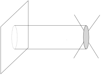
Figure 1: A D1-brane instanton correction to $trF^{4}$.

The Nambu–Goto world-sheet Euclidean action of the D1-brane is known [58] to be

$$S_{D1}={1\over 2\pi\alpha^{\prime}}\int d^{2}\sigma e^{-\Phi/2}\sqrt{|{\rm det}\hat{G}|}-{i\over 2\pi\alpha^{\prime}}\int B\,,$$ (6.1)

where $\hat{G}$ is the induced metric on the world-sheet

$$\hat{G}_{ij}=G_{\mu\nu}\partial_{i}X^{\mu}\partial_{j}X^{\nu}\,,$$ (6.2)

$G_{\mu\nu}$ is the type-I spacetime metric ($\sigma$-model frame), $B$ is the type-I (RR) antisymmetric tensor and the factor $e^{-\Phi/2}$ is due to the fact that the action comes from the disk. The tension $1/2\pi\alpha^{\prime}$ has been computed directly in [59].

We will now evaluate the classical action of the D1-brane wrapped around the target space torus. Using Cartesian coordinates $X^{1},X^{2}\in[0,2\pi]$ for the target space torus and $\sigma_{1,2}\in[0,2\pi]$ for the D1-brane, the $\sigma$-model type-I torus metric is

$$G={\sqrt{{\rm det}G}\over U_{2}}\left(\matrix{1&U_{1}\cr U_{1}&|U|^{2}\cr}\right)\,.$$ (6.3)

The complex structure $U$ defines complex coordinates as usual

$$Z=X^{1}+UX^{2}\;\;\;,\;\;\;\bar{Z}=X^{1}+\overline{U}X^{2}\,.$$ (6.4)

The map that wraps the D1-brane world-sheet around the two-torus is

$$\left(\matrix{X^{1}\cr X^{2}\cr}\right)=\left(\matrix{n_{1}&m_{1}\cr n_{2}&m_{2}\cr}\right)\left(\matrix{\sigma_{1}\cr\sigma_{2}\cr}\right)\,.$$ (6.5)

To have a non-trivial wrapped configuration with the same orientation, $n_{1}m_{2}-n_{2}m_{1}>0$. For $n_{1}m_{2}-n_{2}m_{1}<0$, the orientation is reversed and the induced complex structure is complex-conjugated. As we will see below, the first case corresponds to instantons, the second to anti-instantons.

The complex structure of the original torus (6.4) induces a complex structure of the D1-brane. Defining

$$z=\sigma_{1}+{\cal U}\sigma_{2}\;\;\;,\;\;\;\bar{z}=\sigma_{1}+\overline{{\cal U}}\sigma_{2}$$ (6.6)

the map from $Z$ to $z$ is holomorphic, $Z=f(z)$. If the map changes the orientation, this acts as complex conjugation on the complex structure. Using (6.4) and (6.5) we find that

$$Z=({n_{1}+Un_{2}})\left[\sigma_{1}+{m_{1}+Um_{2}\over n_{1}+Un_{2}}\sigma_{2}\right]\,,$$ (6.7)

which implies that the induced complex modulus is

$${\cal U}={m_{1}+Um_{2}\over n_{1}+Un_{2}}\;\;\;,\;\;\;n_{1}m_{2}-n_{2}m_{1}>0\;\;\;,\;\;\;{\rm Im}\,{\cal U}>0$$ (6.8)

and

$$\;\;\;\;{\cal U}={m_{1}+\overline{U}m_{2}\over n_{1}+\overline{U}n_{2}}\;\;\;,\;\;\;n_{1}m_{2}-n_{2}m_{1}<0\;\;\;,\;\;\;{\rm Im}\,{\cal U}>0\,.$$ (6.9)

Modular transformations of the target-space torus act on $X^{1},X^{2}$ by $SL(2,Z)$ transformations. From (6.5) we deduce that they also act on the matrix of “winding numbers” by left $SL(2,Z)$ transformations. Modular transformations on the D1-brane coordinates $\sigma_{1},\sigma_{2}$, act on the winding number matrix by right modular transformations. Configurations are equivalent if they are related by $SL(2,Z)$ transformations of the D1-brane coordinates $\sigma_{i}$. The reason is that, since we are using the Nambu–Goto type action, we have already “integrated out” the world-sheet metric. Thus, we can use the right $SL(2,Z)$ action to pick representative configurations with

$$\left(\matrix{n_{1}&m_{1}\cr n_{2}&m_{2}\cr}\right)=\left(\matrix{k&j\cr 0&p\cr}\right)\;\;\;,\;\;\;p>0\;\;\quad,\quad 0\leq j<|k|\,.$$ (6.10)

For such configurations ${\cal U}=(pU+j)/k$.

We can now evaluate the D1-brane classical action. Using (6.2), (6.5), (6.10) we find

$$\sqrt{|{\rm det}\hat{G}|}=\sqrt{{\rm det}G}|pk|$$ (6.11a)

$$\int B_{ij}dX^{i}\wedge dX^{j}=pk~{}B_{12}\,.$$ (6.11b)

Denoting also $\lambda_{\rm I}=e^{\Phi/2}$ we obtain

$$S_{\rm class}={2\pi\over\alpha^{\prime}}\left[|pk|{\sqrt{{\rm det}G}\over\lambda_{\rm I}}-ipkB_{12}\right]\,.$$ (6.12)

As described in Appendix B the mapping between heterotic and type-I variables is $\left.T_{1}\right|_{\rm het}=\left.T_{1}\right|_{\rm I}$ , $U_{\rm het}=U_{\rm I}$ and $\left.T_{2}\right|_{\rm het}=\left.T_{2}\over\lambda\right|_{\rm I}$. We can express this in terms of heterotic variables

$$\left.T_{2}\right|_{\rm het}={\sqrt{{\rm det}G}\over\alpha^{\prime}\lambda_{\rm I}}\;\;\;,\;\;\;\left.T_{1}\right|_{\rm het}={B_{12}\over\alpha^{\prime}}$$ (6.13)

to obtain

$$e^{-S_{\rm class}}=\exp\left[-2\pi\left(|pk|T_{2}-ipkT_{1}\right)\right]\,.$$ (6.14)

When $k>0$, we have instantons and

$$e^{-S_{\rm class}}=e^{2\pi ipkT}\,,$$ (6.15)

which is to be summed over $k,p>0$, $0\leq j<k$. For $k<0$, we have anti-instantons and

$$e^{-S_{\rm class}}=e^{-2\pi ipk\overline{T}}\,,$$ (6.16)

which is again to be summed over $k,p>0$, $0\leq j<k$. This precisely matches the instanton expansion on the heterotic side in (4.13).

We now come to the issue of determinants. Since the D1-brane has the same world-sheet structure as the heterotic string [39], we would expect that, up to volume factors, the $\chi=0$ (one-loop) contribution to the determinant should be the heterotic elliptic genus evaluated at the modulus of the wrapped D1-brane, $\tau\to{\cal U}$. This is suggested by the heterotic expansion (4.13) and is also natural on the type-I side. For anti-instantons, $\tau\to\overline{\cal U}$. Finally, there is an overall factor of $\sqrt{{\rm det}G}/\sqrt{{\rm det}\hat{G}}$, the ratio of volumes of the target space torus to the D1-brane torus. This can be understood as follows. The inverse of $\sqrt{{\rm det}\hat{G}}$ is coming from the normalization of zero modes, while the $\sqrt{{\rm det}G}$ factor is the standard volume factor of the target space torus.

This concludes the discussion for the $trF^{4}$ and $trR^{4}$ terms. For the rest, there are extra contributions coming from an instanton calculation for $\chi=-1,-2$. The holomorphic determinants here are related to the heterotic elliptic genus via (4.13) and are the relevant quantities that appear in the calculation of the generalization of the Kähler potential in the $N=4$ case (see Section 5). Moreover, there is an extra overall factor of $({\rm det}\hat{G})^{\chi/2}$ related to zero modes. It would be interesting to directly understand the type-I calculation of these terms.

One final comment is in order here. The world-sheet theory of $N$ D1-branes is a gauge theory with (8,0) supersymmetry in two dimensions. It has an $SO(N)$ gauge group, eight scalars that transform in the symmetric tensor of $SO(N)$ and parametrize the relative distance moduli as well as another eight, which are $SO(N)$ singlets and parametrize the centre-of-mass position in transverse space. These are accompanied by left-moving fermions coming from the DD Ramond sector. There are also DN fermions transforming in the $(N,32)$ under $SO(N)\times SO(32)$. Thus, an $SO(N)$ matrix theory describes the dynamics of $N$ D1-branes, [61]. As was observed in [20], in analogy with the type-II case, we would expect that the IR limit is parametrized by separate coordinates of the $N$ D1-strings, with an orbifold identification when two of them coincide [62]. On the other hand, it was shown in [63] that for symmetric CFTs the elliptic genus of an $S_{N}$ orbifold is given by the action of a Hecke operator of order $N$ on the original elliptic genus. Although this was shown in the type-II context, it is also valid for heterotic orbifolds.

The above discussion provides an interpretation of eq. (4.15), which expresses the instanton sum as a sum over Hecke operators acting on the elliptic genus. The $N$-th term in the sum should come from $N$ D1-brane instanton configurations. This interpretation should be directly derivable from the appropriate matrix model [20].

7 $D=8$ Heterotic Thresholds with
Non-Zero Wilson Lines

We will now include generic Wilson lines $Y^{i}_{I}$, $i=1\ldots 16$, $I=1,2$ which generically break the gauge group to the Cartan, $O(32)\to U(1)^{16}$. We define the following complex moduli

$$G={(2T_{2}U_{2}-\bar{y}_{2}\cdot\bar{y}_{2})\over 2U_{2}^{2}}\pmatrix{1&U_{1}\cr U_{1}&|U|^{2}\cr}\quad,\quad B_{12}=T_{1}-{\bar{y}_{1}\cdot\bar{y}_{2}\over 2U_{2}}$$ (7.1a)

$$y^{i}=(y_{1}+iy_{2})^{i}=-Y_{2}^{i}+UY_{1}^{i}$$ (7.1b)

where we denote with $\bar{y}$ the sixteen-dimensional complex vector of Wilson lines. Note that the volume of the two-torus in this parametrization is

$${\cal V}\equiv\sqrt{\det G}=T_{2}-{\bar{y}_{2}\cdot\bar{y}_{2}\over 2U_{2}}\,.$$ (7.2)

We focus for simplicity on the gravitational one-loop thresholds given in (3.8) and (3.9):

$${\cal I}^{\rm het}_{D=8}=-{\cal N}_{8}\int_{{\cal F}}{d^{2}\tau\over\tau_{2}^{2}}\;(\tau_{2}\Gamma_{2,18}(T,U,\bar{y}))\ \hat{\cal A}({\cal R},\tau)\,.$$ (7.3)

The appropriate elliptic genus for a given term can be written as

$$\hat{{\cal A}}=\sum_{\nu=0}^{\nu_{\rm max}}\hat{E}_{2}^{\nu}\Phi_{\nu}(\tau)\,,$$ (7.4)

where $\nu_{\rm max}=0$ for $trR^{4}$ and $\nu_{\rm max}=2$ for $(trR^{2})^{2}$. Here $\Phi_{\nu}$ is a modular form of weight $-8-2\nu$ and the explicit form of the relevant $\Phi_{\nu}$’s can be read from (3.9). The integral can be done explicitly and the result can be expressed in terms of polylogarithms. This is described in Appendix E. The trivial and degenerate orbits produce a result that is perturbative on the type-I side. The non-degenerate orbits give a result that is non-perturbative on the type-I side. We are interested in the large volume expansion of the non-degenerate orbit contribution. This is derived in Appendix F, and we will reproduce it here. We introduce the $O(32)_{1}$ affine lattice sum

$$\chi(\bar{y}|\tau)=\sum_{\bar{r}}e^{i\pi\tau\bar{r}\cdot\bar{r}}e^{2i\pi\bar{r}\cdot\bar{y}}={1\over 2}\sum_{a,b=0}^{1}\prod_{i=1}^{16}\vartheta[^{a}_{b}](y^{i}|\tau)$$ (7.5)

where $\bar{r}$ is a vector in the Spin(32)/Z₂ lattice. The full affine character is given by $\chi$ divided by $\eta^{16}$. Under modular transformations

$$\chi(\bar{y}+\bar{\epsilon}_{1}+\tau\bar{\epsilon}_{2}|\tau)=e^{-i\pi(\tau\bar{\epsilon}_{2}\cdot\bar{\epsilon}_{2}+2\bar{\epsilon}_{2}\cdot\bar{y})}\chi(\tau,\bar{y})\;\;\;,\;\;\;\chi(\bar{y}|\tau+1)=\chi(\bar{y}|\tau)$$ (7.6a)

$$\chi\left({\bar{y}\over\tau}|-{1\over\tau}\right)=\tau^{8}e^{i\pi{\bar{y}\cdot\bar{y}\over\tau}}\chi(\tau,\bar{y})$$ (7.6b)

where $\bar{\epsilon}_{1,2}$ are lattice vectors. These transformations define a generalized Jacobi form of type $(d,m)=(8,1)$. Properties of such forms are reviewed in Appendix A.2. We will introduce also the covariant derivative on generalized Jacobi forms

$$\tilde{D}=D_{\tau}+{i\over\pi\tau_{2}}\bar{y}_{2}\cdot\partial_{\bar{y}}-m{\bar{y}_{2}\cdot\bar{y}_{2}\over\tau_{2}^{2}}\,,$$ (7.7)

which is such that $\tilde{D}F_{d,m}$ is a Jacobi form of type $(d+2,m)$. $D_{\tau}$ is the usual covariant derivative on weight $d$ modular forms defined in Appendix A.1. We will now define the relatives of the character-valued elliptic genus as

$$\hat{\cal A}_{s}(\bar{y},\tau)=\tilde{D}^{s}\sum_{\nu=s}^{\nu_{\rm max}}\left(\nu\atop s\right)\chi(\bar{y}|\tau)\hat{E}^{\nu-s}_{2}\Phi_{\nu}(\tau)\,,$$ (7.8)

with $\hat{\cal A}_{0}=\chi(\bar{y}|\tau)\hat{\cal A}(\tau)$. Note that by setting the Wilson lines $\bar{y}$ to zero (7.8) reduces to (4.12). The non-degenerate orbit part of the threshold can be written as

$${\cal I}_{\rm inst}=-4{\cal N}_{8}{\rm Re}\sum_{s=0}^{\nu_{\rm max}}\left({3\over 2\pi}\right)^{s}\sum_{{0\leq j<k}\atop{p>0}}{1\over(kp)^{s+1}{\cal V}^{s}}\;e^{2\pi iTpk}\;\hat{\cal A}_{s}\left(p\bar{y},{pU+j\over k}\right)\,.$$ (7.9)

which generalizes the zero Wilson-line result (4.13). It is also written as an expansion in inverse powers of ${\cal V}$, which is the volume of the two-torus (see eq. (7.2)). Using the generalized Hecke operators $V_{N}$ [64] of Appendix A.3, the result can also be recast in the following form:

$${\cal I}_{\rm inst}=-4{\cal N}_{8}{\rm Re}\sum_{s=0}^{\nu_{\rm max}}\left({3\over 2\pi}\right)^{s}\sum_{N=1}^{\infty}{1\over(N{\cal V})^{s}}\;e^{2\pi iNT}V_{N}[\hat{\cal A}_{s}](\bar{y}|U)\,,$$ (7.10)

which is the analogue of (4.15) obtained with zero Wilson lines.

Before we proceed with the D1-instanton interpretation of the result, we should mention that the thresholds in the presence of Wilson lines can also be written in terms of generalized prepotentials. As shown in Appendix E.2, the generalization of (5.24) is

$$\Psi_{s}=-C\delta_{s,0}\log(T_{2}U_{2}-\bar{y}\cdot\bar{y}/2)+\sum_{\nu=s}^{\nu_{\rm max}}{(\nu+s)!\over 6^{s}(\nu-s)!s!}\left[\mathchoice{\vbox{\vbox{\hrule height=0.4pt\hbox{\vrule width=0.4pt,height=6.0pt\kern 6.0pt\vrule width=0.4pt} \hrule height=0.4pt}}}{\vbox{\vbox{\hrule height=0.4pt\hbox{\vrule width=0.4pt,height=6.0pt\kern 6.0pt\vrule width=0.4pt} \hrule height=0.4pt}}}{\vbox{\vbox{\hrule height=0.3pt\hbox{\vrule width=0.3pt,height=2.1pt\kern 2.1pt\vrule width=0.3pt} \hrule height=0.3pt}}}{\vbox{\vbox{\hrule height=0.3pt\hbox{\vrule width=0.3pt,height=1.5pt\kern 1.5pt\vrule width=0.3pt} \hrule height=0.3pt}}}^{\nu}f_{\nu}(T,U,\bar{y})+cc\right]\,,$$ (7.11)

where       acting on a $(d,m)$ Jacobi form is

$$\mathchoice{\vbox{\vbox{\hrule height=0.4pt\hbox{\vrule width=0.4pt,height=6.0pt\kern 6.0pt\vrule width=0.4pt} \hrule height=0.4pt}}}{\vbox{\vbox{\hrule height=0.4pt\hbox{\vrule width=0.4pt,height=6.0pt\kern 6.0pt\vrule width=0.4pt} \hrule height=0.4pt}}}{\vbox{\vbox{\hrule height=0.3pt\hbox{\vrule width=0.3pt,height=2.1pt\kern 2.1pt\vrule width=0.3pt} \hrule height=0.3pt}}}{\vbox{\vbox{\hrule height=0.3pt\hbox{\vrule width=0.3pt,height=1.5pt\kern 1.5pt\vrule width=0.3pt} \hrule height=0.3pt}}}=\frac{1}{2\pi^{2}}\left(\partial_{\bar{y}}\cdot\partial_{\bar{y}}-2\partial_{T}\partial_{U}+{16-2d\over(\bar{y}_{2}\cdot\bar{y}_{2}-2T_{2}U_{2})}\left[\frac{d}{2}+i(\bar{y}_{2}\cdot\partial_{\bar{y}}+T_{2}\partial_{T}+U_{2}\partial_{U})\right]\right)\,.$$ (7.12)

It reduces to $D_{T}D_{U}$ in the absence of Wilson lines. More explicit forms for the generalized prepotentials in this case are given in Appendix E.2.

We will now interpret the result in terms of the D1-brane. The coupling of the D1-brane to bulk gauge fields is a one-loop effect given by the diagram in Fig. 1. Thus, the coupling to Wilson lines is also a one-loop effect; consequently, it is independent of the type-I dilaton. We can evaluate the induced Wilson lines on the D1-brane world-sheet as

$$\bar{w}=-\bar{W}_{2}+{\cal U}\bar{W}_{1}=p\bar{y}$$ (7.13)

where we have used $\bar{W}_{i}=\bar{Y}_{\alpha}\partial_{i}X^{\alpha}$, ${\cal U}=(pU+j)/k$ and the map (6.5), (6.10). This explains the dependence of the generalized elliptic genus in (7.9). Thus, part of the one-loop determinant is the heterotic genus evaluated at the induced world-sheet modulus ${\cal U}$ and the induced Wilson lines $\bar{w}$.

The exponential factor $\exp[2\pi ikpT]$ is composed of two parts. Using (7.1b) we find that the first part is the same as was discussed in Section 6 and that it is generated by the D1-brane classical action. There is a left-over piece depending on the Wilson lines, which after some algebra can be written in terms of induced data as $\exp[i\pi{\bar{w}\cdot\bar{w}_{2}\over{\cal U}_{2}}]$. This is the Quillen anomaly of the one-loop determinant of the 32 world-sheet fermion fluctuations of the D1-brane coupled to the induced Wilson lines $\bar{w}$. There are also the usual factors of volume, as in the case with zero Wilson lines. The terms in (7.9) with $s>0$ correspond to higher-loop contributions around the instanton, on the type-I side. We conclude that the one-loop determinants around the D1-instanton are composed of the heterotic elliptic genus evaluated at $\tau={\cal U}$ multiplied on the one hand by the $O(32)$ affine character evaluated at $\tau={\cal U}$ and at the induced Wilson lines $\bar{y}\to\bar{w}$ and also multiplied by the anomaly factor of the world-sheet fermions. Again we sum over all possible wrappings of the D1-brane, modded out by the world-sheet diffeomorphisms.

Since, here, we can also write the result in terms of the generalized Hecke operators $V_{N}$ as in (7.10), it is this form that should correspond to the D1 matrix model with non-trivial Wilson lines.

8 Heterotic Thresholds in $D<8$

We will now discuss heterotic thresholds in toroidal compactifications to $D<8$. As we argued earlier, if $D>4$ then the heterotic result is still one-loop only and can be evaluated. Using heterotic/type-I duality we find again the non-perturbative type-I corrections and we show that their corresponding D1-brane interpretation is in agreement with the D1-brane rules given in Section 6.

Our starting point is the general form of the one-loop thresholds

$${\cal I}^{\rm het}_{D}=-{\cal N}_{D}\int_{{\cal F}}{d^{2}\tau\over\tau_{2}^{2}}\;(\tau_{2}^{d/2}\Gamma_{d,d}(G,B))\ {\cal A}(\tau)\,,$$ (8.1)

where the $D+d=10$ and the $d$-dimensional lattice sum $\Gamma_{d,d}$ is given by

$$\Gamma_{d,d}(G,B)={\sqrt{G}\over\tau_{2}^{d/2}}\sum_{m^{i},n^{i}\in{Z}}\exp\left[-{\pi\over\tau_{2}}(G+B)_{ij}(m^{i}+n^{i}\tau)(m^{j}+n^{j}\bar{\tau})\right]\,,$$ (8.2)

where $G$ and $B$ are the $d$-dimensional metric and antisymmetric tensor respectively. Alternate forms of the lattice sum can be found in Appendix H.

The corresponding integral (8.1) can be evaluated again, using the method of orbits. We refer to Appendix H for the main steps, and quote here only the result of the non-degenerate orbit, which comprises the type-I instantonic contributions:

$${\cal I}_{\rm inst}=-2{\cal N}_{D}\sum_{s=0}^{\nu_{\rm max}}\left({3\over 2\pi}\right)^{s}\sum_{m,n}^{\prime}{\sqrt{G}\over(T^{m,n}_{2})^{s+1}}e^{2\pi iT^{m,n}}{\cal A}_{s}(U^{m,n})$$ (8.3)

where we have used the definition (4.12) of the elliptic genera. Here, the induced Kähler and complex structure moduli are given by

$$T^{m,n}=mBn+i\sqrt{(mGm)(nGn)-(mGn)^{2}}\;\;\;\;\;\;\;\;\;\;\;\;\;\;\;\;\;$$ (8.4a)

$$U^{m,n}=\left(-mGn+i\sqrt{(mGm)(nGn)-(mGn)^{2}}\;\right)/nGn$$ (8.4b)

and the $\sum_{m,n}^{\prime}$ is over the non-degenerate orbits, which are parametrized by the following integer-valued $2\times d$ matrices

$$\mbox{non-degenerate orbit}:\;\;\;\;A^{T}=\left(\matrix{n_{1}&\ldots&n_{k}&0&\ldots&0\cr m_{1}&\ldots&m_{k}&m_{k+1}&\ldots&m_{d}\cr}\right)\;\;\;\;\;\;\;\;\;\;\;\;\;\;\;\;\;\;\;\;\;\;\;\;\;\;\;\;\;\;\;\;$$ (8.5a)

$$\;\;\;\;\;\;\;\;\;\;\;\;\;\;\;\;\;\;\;\;\;\;\;\;\;\;\;\;\;\;\;\;\;\;1\leq k<d\quad,\quad n_{k}>m_{k}\geq 0\quad,\quad(m_{k+1},\ldots,m_{d})\neq(0,\ldots,0)\,.$$ (8.5b)

Note that for $d=2$ the general result (8.3) reduces to the one given in (4.13).

Turning to the D1-brane interpretation of the result, we first wish to establish that the exponential factor $e^{2\pi iT^{m,n}}$ agrees with the classical action of a D1-brane. The map that describes the wrapping of the D1-brane world-sheet around a 2-cycle in the $d$-torus is

$$X^{i}=n_{i}\sigma_{1}+m_{i}\sigma_{2}\quad,\quad i=1\ldots d\,,$$ (8.6)

where $X^{i}$ are the coordinates on $T^{d}$ and $\sigma_{1,2}$ the D1-brane coordinates. We observe that modular transformations on the D1-brane coordinates act on the matrix $A$ that enters (8.6)

$$A=\left(\matrix{n_{1}&m_{1}\cr\vdots&\vdots\cr n_{d}&m_{d}\cr}\right)$$ (8.7)

by right $SL(2,Z)$ transformations, which forces us to pick the representative configurations described by the matrices in (8.5b).

In terms of the matrix $M_{I}^{i}=(A_{i}^{I})^{T}=(n^{i},m^{i})$, $I=1,2$, we see that the induced metric and antisymmetric tensor fields are

$$\hat{G}_{IJ}=M_{I}^{i}G_{ij}M_{J}^{j}\quad,\quad\hat{B}_{IJ}=M_{I}^{i}B_{ij}M_{J}^{j}\,.$$ (8.8)

In particular, going through the same steps as in Section 6, we find from the D1-brane classical action (6.1) and (8.4b), (8.8) that $e^{-S_{\rm class}}$ precisely reduces to the exponential factor $e^{2\pi iT^{m,n}}$, which is to be summed over the ranges indicated in (8.5b). We also note that we correctly observe the overall factor $\sqrt{G}/\sqrt{\hat{G}}=\sqrt{G}/T^{m,n}_{2}$. Moreover, the fluctuation determinant is evaluated at the induced modulus $U^{m,n}$ of the wrapped D1-brane.

This establishes the claim that the D1-brane rules in $D<8$ are consistent with those obtained for $D=8$. In summary, we have found the intuitively expected result that the instantonic contributions consist of all possible inequivalent wrappings of the D1-brane around two-tori that are embedded in the $d$-dimensional target space torus modulo reparametrizations of the D1-brane world-sheet.

In the eight-dimensional case we have shown that differential equations satisfied by the (2,2) toroidal lattice sum translate into recursion relations for the thresholds, which can be solved in terms of holomorphic prepotentials. There is a generalization of such equations for the $(d,d)$ toroidal lattice sum.

It was noted in Refs. [50, 65] that the toroidal partition function $\Gamma_{d,d}(G,B;\tau)$ satisfies the following differential equation:

$$\left[\left(\sum_{i\leq j}G_{ij}{\partial\over\partial G_{ij}}+{1-d\over 2}\right)^{2}+\frac{1}{2}\sum_{ijkl}G_{ik}G_{jl}{\partial^{2}\over\partial B_{ij}\partial B_{kl}}-\frac{1}{4}-4\tau_{2}^{2}{\partial^{2}\over\partial\tau\partial\bar{\tau}}\right]\Gamma_{d,d}(G,B;\tau)=0$$ (8.9)

which in the case $d=2$ reduces to

$$\left[T_{2}^{2}\partial_{T}\partial_{\bar{T}}-\tau_{2}^{2}\partial_{\tau}\partial_{\bar{\tau}}\right]\Gamma_{2,2}(T,U;\tau)=0\,.$$ (8.10)

However, the general differential equation in (8.9) is not invariant under the full $O(d,d,Z)$ duality group. It may be verified that it is invariant under integer $B$ shifts and $SL(d,Z)$ basis changes, but there is no invariance under the remaining generators of the duality group, which are the inversion and factorized duality. The latter two transformations act on the matrix $E\equiv G+B$ as follows:

$$E\rightarrow E^{-1}\quad,\quad E\rightarrow[(1-e_{i})E+e_{i}][e_{i}E+(1-e_{i})]^{-1}\quad,\quad(e_{i})_{k,l}=\delta_{ik}\delta_{il}\,.$$ (8.11)

For example, in the $d=2$ case the factorized dualities correspond to $T\rightarrow U$ and $T\rightarrow 1/U$ for $i=1$ and 2 respectively, which do not leave the differential equation in (8.10) invariant.

This implies that there must be further constraints on $\Gamma_{d,d}$ generalizing the $d=2$ relation

$$\left[T_{2}^{2}\partial_{T}\partial_{\bar{T}}-U_{2}^{2}\partial_{U}\partial_{\bar{U}}\right]\Gamma_{2,2}(T,U;\tau)=0\,.$$ (8.12)

To find the generalization of this relation we note that there is another $O(d,d,Z)$ invariant differential equation on the lattice sum, which reads

$$\left[\sum_{ijkl}G_{ik}G_{jl}{\partial^{2}\over\partial E_{ij}\partial E_{kl}}+\sum_{ij}G_{ij}{\partial\over\partial E_{ij}}+\frac{1}{4}d(d-2)-4\tau_{2}^{2}\partial_{\tau}\partial_{\bar{\tau}}\right]\Gamma_{d,d}(E;\tau)=0\,.$$ (8.13)

As a consequence we find that the difference between (8.9) and (8.13) is the differential equation,

$$\left[\sum_{ijkl}(G_{ij}G_{kl}-G_{jk}G_{il}){\partial^{2}\over\partial E_{ij}\partial E_{kl}}+(1-d)\sum_{ij}G_{ij}{\partial\over\partial E_{ij}}\right]\Gamma_{d,d}(E;\tau)=0\,,$$ (8.14)

which, for $d=2$, turns out to precisely reduce to (8.12). In fact, there is an entire family of constraints

$$\left[\sum_{ijkl}(P_{ij}P_{kl}-P_{kj}P_{il}){\partial^{2}\over\partial E_{ij}\partial E_{kl}}+\sum_{ij}[(PG^{-1}-{\rm Tr}(PG^{-1}){\mathchoice{\rm 1\mskip-4.0mul}{\rm 1\mskip-4.0mu}{\rm 1\mskip-4.5mul}{\rm 1\mskip-5.0mul}})P]_{ij}{\partial\over\partial E_{ij}}\right]\Gamma_{d,d}(E;\tau)=0\,,$$ (8.15)

which include (8.14) for $P=G$. Here $P$ is an arbitrary matrix.

Clearly (8.14) and its generalization (8.15) are not invariant under the duality group, since (as (8.9)) the inversion and factorized duality are broken, but these transformations should be used to form a complete irreducible set of differential equations. For example, under the inversion, we find that (8.15) with matrix $P$ is transformed into the same differential equation with matrix

$$P^{\prime}=E\tilde{P}E\quad,\quad\tilde{P}=P|_{E\rightarrow E^{-1}}\,.$$ (8.16)

It is an open problem to find the general solution of such equations which will define the analog of prepotentials in the lower dimensional case.

9 Conclusions and Remarks

We have analyzed here heterotic/type-I duality in eight dimensions with arbitrary Wilson lines as well as in $D<8$ dimensions with zero Wilson lines.

We focused in particular on $R^{4}$ terms in the effective action that obtain corrections from short multiplets.

In eight dimensions, the heterotic result is one-loop only. However, non-perturbative instanton corrections are necessary on the type-I side. We identified the relevant instanton configurations with a D1-brane wrapped around the compact two-torus. The heterotic result implies a concrete way to count different instanton configurations. Multiple overlapping D1-branes have to be included, however, in order to restore $T$-duality. Moreover, we have to sum over D1-branes wrapped in any possible way around ${\cal T}^{2}$ modulo the modular transformations of the D1-world-volume. Most interestingly, the fluctuation determinant around a given D1-instanton configuration is given by the heterotic elliptic genus evaluated at the complex structure modulus induced on the world-sheet of the wrapped D1-brane. The instanton result can be written in terms of Hecke operators. In this form it provides a potentially interesting link with a $SO(N)$ matrix model of D1-branes. Finally, we have shown that the thresholds can be expressed in terms of generalized holomorphic prepotentials.

We have also considered the heterotic perturbative thresholds in $D=8$ in the presence of arbitrary Wilson lines. We have calculated exactly the one-loop perturbative contribution. In this case, heterotic/type-I duality predicts that the D1-instanton determinant is the affine character-valued genus evaluated at the induced complex structure of the D1-brane world-volume and the induced Wilson lines on this world-sheet. Moreover, we found the exponential factors to be in agreement with the classical D1-brane action as well as the Quillen anomaly of the 32 fermions.

Finally, we have discussed the heterotic perturbative thresholds in toroidal compactifications to $D<8$. In this case, again using heterotic/type-I duality, we find agreement with the D1-brane rules obtained from $D=8$. In particular, we observe all possible wrappings of the D1-brane around the various two-tori that are embedded in the $d$-torus. Moreover, the exponential factor corresponding to the classical action as well as the fluctuation determinants are in agreement with the $D=8$ result as well.

There are several questions, however, that remain open. An essential quantitative test of heterotic/type-I duality can be obtained by directly calculating relevant higher-genus terms on the type-I side. Already in ten dimensions, the $\chi=-1$, $(trF^{2}-trR^{2})^{2}$ term should match the corresponding tree-level term on the heterotic side. In $D<10$, further higher-genus contact terms, corresponding to one-loop world-sheet contact terms on the heterotic side, should be checked. This state of affairs in duality comparisons is not new. Similar situations arise in $N=2$ heterotic/type-II dual pairs with $N=2$ supersymmetry, and heterotic/type-I dual pairs with $N=2$ supersymmetry.

At the effective supergravity level, knowledge of the holomorphic ($D=8$) or quaternionic ($D=6$) structure of the special derivative terms is missing. An analogue of the higher F-terms of $N=2$ supersymmetry should exist for $N=4$ supersymmetry. The expressions that we have obtained in Appendix E.2 for the heterotic thresholds in terms of generalized prepotentials are very suggestive in this respect.

Since our results on the heterotic side are supposed to be non-perturbatively exact for $D>4$, a direct quantitative check could be made of the conjectured F-theory/heterotic duality in eight dimensions [60]. Techniques however are necessary on the F-theory side to calculate the relevant amplitudes.

The heterotic result can provide a (missing) quantitative test of string–string duality in six dimensions. The type-IIA theory compactified on $K3$ down to six dimensions is conjectured to be equivalent to the heterotic string compactified on ${\cal T}^{4}$. As in the heterotic case, we do not expect non-perturbative corrections either on the type-II side for the $F^{4},R^{4},R^{2}F^{2}$ terms. This can be seen as follows: the relevant D$p$-branes of the ten-dimensional IIA theory have $p=0,2,4,6,8$ with world-sheets being $1,3,5,7,9$-dimensional. To obtain an instanton contribution we need appropriate supersymmetric cycles on $K3$ with dimension belonging to the list above. It is known that there are no such cycles. Moreover, we also have the five-brane, which is magnetically coupled to the NS-NS antisymmetric tensor. Since its world-sheet is six-dimensional it can only give instanton corrections in $D<5$ dimensions. Thus, in $D=6$, heterotic/type-II duality can be tested for the special terms in perturbation theory. Preliminary investigation suggests that the relevant objects on the type-II side are the $N=4$ topological amplitudes defined in [18]. Preliminary investigation shows that for example the tree-level $F^{4}$ terms on the type-II side match the one-loop corrections to such terms on the heterotic side as required by duality. We can further compactify both theories on a circle to five dimensions. There are still no non-perturbative corrections on the heterotic side. In the type-II theory, we expect instanton corrections from the D2- and D4-branes, which are electrically (magnetically) charged under the 3-form. The D2-brane can wrap around ${\cal S}^{1}$ and a supersymmetric two-cycle of $K3$. The D4-brane can wrap on ${\cal S}^{1}$ and the whole of $K3$. These non-perturbative type-II corrections are expected to reproduce the heterotic cross-terms coupling the (4,4) and the (1,1) lattice. A more thorough investigation is needed, however.

Finally, although we do think that we understand the conceptual rules of instanton calculations in string theory, there are several issues that remain to be answered in this respect. A direct D-brane calculation of the D1-instanton determinant should be done. Such techniques are also of importance for five-brane instanton calculations in four-dimensional ground states. Knowing how to do this calculation for the D5-brane will provide, via various dualities, the rules for NS5-brane instantons in heterotic and type-II string theory.

Acknowledgements

This research was partially supported by EEC grant TMR-ERBFMRXCT96-0090. N. Obers acknowledges the hospitality of the Niels Bohr institute during part of this work. We thank C. Bachas and P. Vanhove for participating in the earlier stages of this project and for numerous discussions and insights. We would also like to thank M. Henningson for contributing to the threshold evaluation in $D<8$.

Appendix A Modular functions

A.1 $SL(2,Z)$ modular functions and covariant derivatives

We list in this appendix the $\vartheta$-function definitions we use, and those associated with modular forms. We also discuss modular-covariant derivatives and a number of identities involving these.

Our conventions for the $\vartheta$-function are

$$\vartheta[^{a}_{b}](v|\tau)=\sum_{p\in{Z}}e^{\pi i\tau\left(p-{a\over 2}\right)^{2}+2\pi i\left(v-{b\over 2}\right)\left(p-{a\over 2}\right)}$$ (A.1)

so that the Jacobi $\vartheta$-functions are given by

$$\vartheta_{1}=\vartheta[^{1}_{1}]\quad,\quad\vartheta_{2}=\vartheta[^{1}_{0}]\quad,\quad\vartheta_{3}=\vartheta[^{0}_{0}]\quad,\quad\vartheta_{4}=\vartheta[^{0}_{1}]\,,$$ (A.2)

and the Dedekind function is

$$\eta(\tau)=q^{1/24}\prod_{n=1}^{\infty}(1-q^{n})$$ (A.3)

where $q=e^{2i\pi\tau}$.

Holomorphic modular forms $F_{d}(\tau)$ of weight $d$ transform under the modular group as

$$F_{d}(\tau+1)=F_{d}(\tau)\quad,\quad F_{d}(-1/\tau)=\tau^{d}~{}F_{d}(\tau)$$ (A.4)

A set of modular forms, relevant for our purposes, are the Eisenstein series

$$E_{2k}=-{(2k)!\over(2\pi i)^{2k}B_{2k}}\ G_{2k}\ ,$$ (A.5)

with $B_{2k}$ the Bernoulli numbers and

$$G_{2k}(\tau)=\sum_{(m,n)\not=0}\ (m\tau+n)^{-2k}$$ (A.6)

for $k>1$. For $k=1$ the Eisenstein series diverges. Its modular-invariant regularization, denoted with a hat and used in this paper, is

$${\hat{G}}_{2}(\tau)=\smash{\mathop{\rm lim}\limits_{s\to 0}}\sum_{(m,n)\not=0}\ (m\tau+n)^{-2}|m\tau+n|^{-s}\,.$$ (A.7)

The (hatted) Eisenstein series are modular forms of weight $2k$. The ring of holomorphic modular forms is generated by $E_{4}$ and $E_{6}$. If we include (non-holomorphic) covariant derivatives (to be discussed below) then the generators of this ring are $\hat{E}_{2}$, $E_{4}$, $E_{6}$.

Expressed as power series in $q$, the first few of the Eisenstein series are

$$E_{2}(q)={12\over i\pi}\partial_{\tau}\log\eta=1-24\sum_{n=1}^{\infty}{n\,q^{n}\over 1-q^{n}}\,\$$ (A.8a)

$$E_{4}(q)={1\over 2}\left({\vartheta}_{2}^{8}+{\vartheta}_{3}^{8}+{\vartheta}_{4}^{8}\right)=1+240\sum_{n=1}^{\infty}{n^{3}q^{n}\over 1-q^{n}}\,\$$ (A.8b)

$$E_{6}(q)=\frac{1}{2}\left({\vartheta}_{2}^{4}+{\vartheta}_{3}^{4}\right)\left({\vartheta}_{3}^{4}+{\vartheta}_{4}^{4}\right)\left({\vartheta}_{4}^{4}-{\vartheta}_{2}^{4}\right)=1-504\sum_{n=1}^{\infty}{n^{5}q^{n}\over 1-q^{n}}\,.$$ (A.8c)

The modified first Eisenstein series is

$${\hat{E}}_{2}=E_{2}-{3\over\pi\tau_{2}}\,.$$ (A.9)

We can write the (weight 12) cusp form $\eta^{24}$ and the modular-invariant $j$-function in terms of $E_{4}$ and $E_{6}$

$$\eta^{24}={1\over 2^{6}\cdot 3^{3}}\left[E_{4}^{3}-E_{6}^{2}\right]\;\;\;,\;\;\;j={E_{4}^{3}\over\eta^{24}}={1\over q}+744+{\cal O}(q)\,.$$ (A.10)

There is a (non-holomorphic) covariant derivative that maps modular forms of weight $d$ to forms of weight $d+2$, defined as

$$F_{d+2}=\left({i\over\pi}\partial_{\tau}+{d/2\over\pi\tau_{2}}\right)F_{d}=-2\left(q\partial_{q}-{d\over 4\pi\tau_{2}}\right)F_{d}\equiv D_{d}\;F_{d}\,.$$ (A.11)

The covariant derivative satisfies the distributive property

$$D_{d_{1}+d_{2}}~{}(F_{d_{1}}~{}F_{d_{2}})=F_{d_{2}}(D_{d_{1}}F_{d_{1}})+F_{d_{1}}(D_{d_{2}}F_{d_{2}})\,.$$ (A.12)

We will suppress the index $d$ from the covariant derivative and write multiple derivatives as $D^{n}$. For example a double derivative on a weight $d$ form is

$$D^{2}F_{d}\equiv\left({i\over\pi}\partial_{\tau}+{(d+2)/2\over\pi\tau_{2}}\right)\left({i\over\pi}\partial_{\tau}+{d/2\over\pi\tau_{2}}\right)F_{d}\,.$$ (A.13)

The following formulae allow the computation of the covariant derivative of any form:

$$D\;\hat{E}_{2}={1\over 6}E_{4}-{1\over 6}\hat{E}_{2}^{2}\;\;\;,\;\;\;D\;E_{4}={2\over 3}E_{6}-{2\over 3}\hat{E}_{2}\;E_{4}$$ (A.14a)

$$D\;E_{6}=E_{4}^{2}-\hat{E}_{2}\;E_{6}\,.$$ (A.14b)

There is also a holomorphic covariant derivative on forms of weight $d$: the quantity

$$F_{d+2}=\left({i\over\pi}\partial_{\tau}+{d\over 6}E_{2}\right)F_{d}\equiv\hat{D}_{d}\;F_{d}$$ (A.15)

is a modular form of weight $d+2$. It satisfies a distributive property similar to that in (A.12). For the difference between the two covariant derivatives, we obtain:

$$\hat{D}_{d}-D_{d}={d\over 6}\hat{E}_{2}\,.$$ (A.16)

We also list a number of identities involving modular forms and covariant derivatives, which are used in Appendices E and F. In these expressions the quantity $D^{s}$ always stands for $D_{-2}D_{-4}\cdots D_{-2s}$.
1) Expansion formula

$$(D^{s}\hat{E}_{2}^{\nu-s}\Phi_{\nu})(\tau)=\sum_{r=0}^{s}\sum_{m=0}^{\nu-s}a^{\nu,s}_{r,m}{1\over(\pi\tau_{2})^{s+m-r}}(q\partial_{q})^{r}E_{2}^{\nu-s-m}\Phi_{\nu}(\tau)$$ (A.17a)

 

$${a^{\nu,s}_{r,m}}$$

  (A.17b)

Two useful special cases are

$${\rm Re}D^{s}i\tau^{2s+1}=-{(-2)^{s}s!\over\pi^{s}}\tau_{2}^{s+1}\quad,\quad D^{s}1={(2s)!\over(-2)^{s}s!\pi^{s}}\frac{1}{\tau_{2}^{s}}\,.$$ (A.18)

2) A special function and its derivatives. The following combined polylogarithm functions $L_{(s)}$ play a very special role in the modular-invariant integrals of Appendix E. Their definition is

$$L_{(s)}(x)\equiv\sum_{r=0}^{s}{(s+r)!\over r!(s-r)!(4\pi)^{r}}({\rm Im}\,x)^{s-r}Li_{s+r+1}(e^{2\pi ix})\,,$$ (A.19)

where

$$Li_{s}(x)=\sum_{p=1}^{\infty}\frac{1}{p^{s}}x^{p}$$ (A.20)

are the polylogarithm functions. They satisfy the interesting relations that,

$$D_{U}^{s}D_{T}^{s}Li_{2s+1}(q_{T}^{k}q_{U}^{l})=\sum_{m=0}^{s}{(s+m)!\over m!(s-m)!}(4kl)^{s-m}{L_{(m)}(Tk+Ul)\over(\pi T_{2}U_{2})^{m}}$$ (A.21)

and their inversion

$${L_{(s)}(Tk+Ul)\over(\pi T_{2}U_{2})^{s}}=\sum_{m=0}^{s}{s!\over(s-m)!}{2m+1\over(s+m+1)!}(-4kl)^{s-m}D_{U}^{m}D_{T}^{m}Li_{2m+1}(q_{T}^{k}q_{U}^{l})\,.$$ (A.22)

A.2 Generalized Jacobi forms and covariant derivatives

We give in this appendix a generalization of Jacobi forms [64] and their associated modular-covariant derivatives, and give various properties and application to characters.

We define a generalized Jacobi form of type $(d,m)$ to be a holomorphic function $F_{d,m}(y^{i}|\tau)$ ($i=1\ldots S$) with the following transformation properties

$$F_{d,m}(y^{i}+\epsilon^{i}|\tau)=F_{d,m}(y^{i}|\tau)$$ (A.23a)

$$F_{d,m}(y^{i}+\tau\epsilon^{i}|\tau)=e^{-i\pi m(\tau\epsilon\cdot\epsilon+2\epsilon\cdot y)}F_{d,m}(y^{i}|\tau)$$ (A.23b)

$$F_{d,m}(y^{i},\tau+1)=F_{d,m}(y^{i},\tau)$$ (A.23c)

$$F_{d,m}(y^{i}/\tau|-1/\tau)=\tau^{d}~{}e^{i\pi my\cdot y/\tau}F_{d,m}(y^{i}|\tau)\,,$$ (A.23d)

where $\epsilon^{i}$ is a vector in the lattice $\Gamma^{S,0}$. For our purposes, this will generally be one of the even self-dual Euclidean lattices, which are the $E_{8}$ root lattice with $S=8$ or the root lattice of $E_{8}\times E_{8}$ or weight lattice of ${\rm Spin}(32)/Z_{2}$ with $S=16$.

Then it can be explicitly verified that there exists the following non-holomorphic covariant derivative

$$\tilde{D}=D_{\tau}+{i\over\pi\tau_{2}}\bar{y}_{2}\cdot\partial_{\bar{y}}-m{\bar{y}_{2}\cdot\bar{y}_{2}\over\tau_{2}^{2}}\,,$$ (A.24)

which is such that $\tilde{D}F_{d,m}$ is a Jacobi form of type $(d+2,m)$. Here $D_{\tau}$ is the usual $SL(2,Z)$ covariant derivative (A.11) on a weight $d$ modular function, and $\bar{y}_{2}$ stands for the imaginary part of the $S$-dimensional vector $\bar{y}$. The inner product on this space is taken with the metric $\eta_{(S)}$ on $\Gamma^{S,0}$.

The generators of $O(S+2,2,Z)$ transformations are

$$U\rightarrow U+1\quad,\quad T\rightarrow T\quad,\quad\bar{y}\rightarrow\bar{y}$$ (A.25a)

$$U\rightarrow-1/U\quad,\quad T\rightarrow T-{\bar{y}\cdot\bar{y}\over 2U}\quad,\quad\bar{y}\rightarrow\bar{y}/U$$ (A.25b)

$$U\rightarrow U\quad,\quad T\rightarrow T+\bar{\epsilon}\cdot\bar{y}+\frac{1}{2}\bar{\epsilon}^{2}U\quad,\quad\bar{y}\rightarrow\bar{y}+\bar{\epsilon}U$$ (A.25c)

$$U\rightarrow U\quad,\quad T\rightarrow T\quad,\quad\bar{y}\rightarrow\bar{y}+\bar{\epsilon}$$ (A.25d)

$$U\rightarrow T\quad,\quad T\rightarrow U\quad,\quad\bar{y}\rightarrow\bar{y}$$ (A.25e)

$$U\rightarrow U\quad,\quad T\rightarrow T+1\quad,\quad\bar{y}\rightarrow\bar{y}$$ (A.25f)

$$U\rightarrow U-{\bar{y}\cdot\bar{y}\over 2T}\quad,\quad T\rightarrow-1/T\quad,\quad\bar{y}\rightarrow\bar{y}/T\,.$$ (A.25g)

Note that the first four of these transformations, which leave the variable ${\cal V}=T_{2}-{\bar{y}_{2}\bar{y}_{2}\over 2U_{2}}$ invariant, are the ones used in (A.23d) (ignoring $T$). A function $F_{d}(\bar{y},T,U)$ is of weight $d$ in both $T$ and $U$ if it transforms with a factor $U^{d}$ and $T^{d}$ under the transformations (A.25b) and (A.25g) respectively, and is invariant under the remaining transformations in (A.25g).

We introduce the following notation for the $O(S+2,2)$ moduli,

$$y^{a}=(y^{i},y^{+},y^{-})=(\bar{y},T,U)\quad,\quad\eta^{ab}=\left(\matrix{\eta_{(S)}^{ij}&0\cr 0&-\eta_{(2)}\cr}\right)\quad,\quad\eta_{(2)}=\left(\matrix{0&1\cr 1&0\cr}\right)\,,$$ (A.26)

where $\eta_{(S)}$ is the metric on the lattice, generally taken to be unity. Inner products on this $(S+2)$-dimensional space are taken with the above metric and denoted by $(,)$, so that, for example

$$(y_{2},y_{2})=\bar{y}_{2}\cdot\bar{y}_{2}-2T_{2}U_{2}\,.$$ (A.27)

On the space of $O(S+2,2,Z)$ covariant functions, we define the following operator

$$\mathchoice{\vbox{\vbox{\hrule height=0.4pt\hbox{\vrule width=0.4pt,height=6.0pt\kern 6.0pt\vrule width=0.4pt} \hrule height=0.4pt}}}{\vbox{\vbox{\hrule height=0.4pt\hbox{\vrule width=0.4pt,height=6.0pt\kern 6.0pt\vrule width=0.4pt} \hrule height=0.4pt}}}{\vbox{\vbox{\hrule height=0.3pt\hbox{\vrule width=0.3pt,height=2.1pt\kern 2.1pt\vrule width=0.3pt} \hrule height=0.3pt}}}{\vbox{\vbox{\hrule height=0.3pt\hbox{\vrule width=0.3pt,height=1.5pt\kern 1.5pt\vrule width=0.3pt} \hrule height=0.3pt}}}_{d}=\frac{1}{2\pi^{2}}\left(\eta^{ab}\partial_{y_{a}}\partial_{y_{b}}+{S-2d\over(y_{2},y_{2})}\left[\frac{d}{2}+iy_{2}^{a}\partial_{y_{a}}\right]\right)\,,$$ (A.28)

which satisfies the property that when $F_{(d)}(\bar{y},T,U)$ is a function of weight $d$ in $T$ and $U$, then the function $\mathchoice{\vbox{\vbox{\hrule height=0.4pt\hbox{\vrule width=0.4pt,height=6.0pt\kern 6.0pt\vrule width=0.4pt} \hrule height=0.4pt}}}{\vbox{\vbox{\hrule height=0.4pt\hbox{\vrule width=0.4pt,height=6.0pt\kern 6.0pt\vrule width=0.4pt} \hrule height=0.4pt}}}{\vbox{\vbox{\hrule height=0.3pt\hbox{\vrule width=0.3pt,height=2.1pt\kern 2.1pt\vrule width=0.3pt} \hrule height=0.3pt}}}{\vbox{\vbox{\hrule height=0.3pt\hbox{\vrule width=0.3pt,height=1.5pt\kern 1.5pt\vrule width=0.3pt} \hrule height=0.3pt}}}F_{(d)}(\bar{y},T,U)$ is of weight $d+2$ in both $T$ and $U$. Also note that for $\bar{y}=0$, $S=0$ the operator       reduces to the double covariant derivative $D_{U}D_{T}$.

We also recall the definition of character and affine character lattice sums

$$\chi(\tau)=\sum_{\bar{r}}q^{\bar{r}\cdot\bar{r}/2}\quad,\quad\chi(\bar{y}|\tau)=\sum_{\bar{r}}q^{\bar{r}\cdot\bar{r}/2}e^{2\pi i\bar{r}\cdot\bar{y}}$$ (A.29)

where $\bar{r}$ runs over the appropriate lattice. For example, when $\bar{r}\in\Gamma^{S,0}$, we have for the two relevant cases, $S=8$ and $S=16$, the affine character lattice sums

$$\chi_{E_{8}}(\bar{y}|\tau)={1\over 2}\sum_{a,b=0}^{1}\prod_{i=1}^{8}\theta[^{a}_{b}](y^{i}|\tau)$$ (A.30a)

$$\chi_{E_{8}\times E_{8}}(\bar{y}|\tau)={1\over 2}\sum_{a,b=0}^{1}\prod_{i=1}^{8}\theta[^{a}_{b}](y_{(1)}^{i}|\tau){1\over 2}\sum_{a,b}\prod_{i=1}^{8}\theta[^{a}_{b}](y_{(2)}^{i}|\tau)$$ (A.30b)

$$\chi_{S0(32)}(\bar{y}|q)={1\over 2}\sum_{a,b=0}^{1}\prod_{i=1}^{16}\theta[^{a}_{b}](y^{i}|\tau)\,.$$ (A.30c)

Comparison of the transformation properties of these affine character lattice sums and (A.23d) shows that that they are in fact Jacobi forms of weight $(S/2,1)$. The full affine characters are obtained from the lattice sums by dividing by $\eta^{S}$.

Some identities satisfied by the operators $\tilde{D}$ and       are given below. All of these expressions have been explicitly checked for $s\leq 2$, which covers the cases needed for this paper. We conjecture, however, that they are valid generally, and as a non-trivial check one may verify that they correctly reduce to the identities given in (A.21), (A.22) for $S=0$. Below, the quantities $\tilde{D}^{s}$ stand for $\tilde{D}_{-2}\tilde{D}{-4}\cdots\tilde{D}_{-2s}$ and similarly for $\mathchoice{\vbox{\vbox{\hrule height=0.4pt\hbox{\vrule width=0.4pt,height=6.0pt\kern 6.0pt\vrule width=0.4pt} \hrule height=0.4pt}}}{\vbox{\vbox{\hrule height=0.4pt\hbox{\vrule width=0.4pt,height=6.0pt\kern 6.0pt\vrule width=0.4pt} \hrule height=0.4pt}}}{\vbox{\vbox{\hrule height=0.3pt\hbox{\vrule width=0.3pt,height=2.1pt\kern 2.1pt\vrule width=0.3pt} \hrule height=0.3pt}}}{\vbox{\vbox{\hrule height=0.3pt\hbox{\vrule width=0.3pt,height=1.5pt\kern 1.5pt\vrule width=0.3pt} \hrule height=0.3pt}}}^{s}$.
1) Expansion formula

 

$${(\tilde{D}^{s}\hat{E}_{2}^{\nu-s}\chi(\bar{y})\Phi_{\nu})(\tau)}$$

  (A.31a)

$$\alpha^{\nu,s}_{r,m,p,n}=(-1)^{s+m}{3^{m}4^{r}2^{n}\over 2^{s}}{s!\over r!n!}\left(\nu-s\atop m\right)\left(2s+m-r-n\atop s+m\right)\left(r\atop p\right)$$ (A.31b)

$$0\leq s\leq\nu\quad,\quad 0\leq r\leq s\quad,\quad 0\leq m\leq\nu-s\quad,\quad 0\leq p\leq r\quad,\quad 0\leq n\leq s-r$$

where $\chi(\bar{y}|\tau)$ is the affine character (A.29) of weight $(S/2,1)$.
2) Covariant derivatives of special functions. The combined polylogarithm function defined in (A.19) also satisfies

$$\mathchoice{\vbox{\vbox{\hrule height=0.4pt\hbox{\vrule width=0.4pt,height=6.0pt\kern 6.0pt\vrule width=0.4pt} \hrule height=0.4pt}}}{\vbox{\vbox{\hrule height=0.4pt\hbox{\vrule width=0.4pt,height=6.0pt\kern 6.0pt\vrule width=0.4pt} \hrule height=0.4pt}}}{\vbox{\vbox{\hrule height=0.3pt\hbox{\vrule width=0.3pt,height=2.1pt\kern 2.1pt\vrule width=0.3pt} \hrule height=0.3pt}}}{\vbox{\vbox{\hrule height=0.3pt\hbox{\vrule width=0.3pt,height=1.5pt\kern 1.5pt\vrule width=0.3pt} \hrule height=0.3pt}}}^{s}Li_{2s+1}(e^{2\pi i(r,y)})=\sum_{m=0}^{s}\left(s\atop m\right){(S/2+s+m)!\over(S/2+s)!}(-2)^{s}(r^{2})^{s-m}{L_{(m)}((r,y))\over(\pi(y_{2},y_{2}))^{m}}\,,$$ (A.32)

where $r=(\bar{r},-l,-k)$ so that $(r,y)=\bar{r}\cdot\bar{y}+Tk+Ul$ and $r^{2}=\bar{r}\cdot\bar{r}-2kl$. The inverse of this relation is

$${L_{(s)}((r,y))\over(\pi(y_{2},y_{2}))^{s}}=\sum_{m=0}^{s}\left(s\atop m\right){(S/2+m)!(S/2+2m+1)\over(S/2+s+m+1)!}{(-1)^{s}\over 2^{m}}(r^{2})^{s-m}\mathchoice{\vbox{\vbox{\hrule height=0.4pt\hbox{\vrule width=0.4pt,height=6.0pt\kern 6.0pt\vrule width=0.4pt} \hrule height=0.4pt}}}{\vbox{\vbox{\hrule height=0.4pt\hbox{\vrule width=0.4pt,height=6.0pt\kern 6.0pt\vrule width=0.4pt} \hrule height=0.4pt}}}{\vbox{\vbox{\hrule height=0.3pt\hbox{\vrule width=0.3pt,height=2.1pt\kern 2.1pt\vrule width=0.3pt} \hrule height=0.3pt}}}{\vbox{\vbox{\hrule height=0.3pt\hbox{\vrule width=0.3pt,height=1.5pt\kern 1.5pt\vrule width=0.3pt} \hrule height=0.3pt}}}^{m}Li_{2m+1}(e^{2\pi i(r,y)})\,.$$ (A.33)

We also have the following identity

 

$${{\rm Re}\mathchoice{\vbox{\vbox{\hrule height=0.4pt\hbox{\vrule width=0.4pt,height=6.0pt\kern 6.0pt\vrule width=0.4pt} \hrule height=0.4pt}}}{\vbox{\vbox{\hrule height=0.4pt\hbox{\vrule width=0.4pt,height=6.0pt\kern 6.0pt\vrule width=0.4pt} \hrule height=0.4pt}}}{\vbox{\vbox{\hrule height=0.3pt\hbox{\vrule width=0.3pt,height=2.1pt\kern 2.1pt\vrule width=0.3pt} \hrule height=0.3pt}}}{\vbox{\vbox{\hrule height=0.3pt\hbox{\vrule width=0.3pt,height=1.5pt\kern 1.5pt\vrule width=0.3pt} \hrule height=0.3pt}}}^{s}id^{(s)}_{a_{1}\ldots a_{2s+1}}}$$

  (A.34)

where the tensors $d^{(m)}$ are totally symmetric and recursively defined from $d^{(s)}$ by

$$d^{(m-1)}_{a_{1}\ldots a_{2m-1}}=d^{(m)}_{a_{1}\ldots a_{2m+1}}\eta^{a_{2m}a_{2m+1}}\quad,\quad 1\leq m\leq s\,.$$ (A.35)

The inverse relation reads

$${d^{(s)}_{a_{1}\ldots a_{2s+1}}\over(y_{2},y_{2})^{s}}y_{2}^{a_{1}}\cdots y_{2}^{a_{2s+1}}=-\sum_{m=0}^{s}\left(s\atop m\right){(S/2+m)!(S/2+2m+1)\over(S/2+s+m+1)!}{(-2\pi^{2})^{m}(2s+1)!\over 4^{s}s!(2m+1)!}$$ (A.36)

$$\times{\rm Re}\,\mathchoice{\vbox{\vbox{\hrule height=0.4pt\hbox{\vrule width=0.4pt,height=6.0pt\kern 6.0pt\vrule width=0.4pt} \hrule height=0.4pt}}}{\vbox{\vbox{\hrule height=0.4pt\hbox{\vrule width=0.4pt,height=6.0pt\kern 6.0pt\vrule width=0.4pt} \hrule height=0.4pt}}}{\vbox{\vbox{\hrule height=0.3pt\hbox{\vrule width=0.3pt,height=2.1pt\kern 2.1pt\vrule width=0.3pt} \hrule height=0.3pt}}}{\vbox{\vbox{\hrule height=0.3pt\hbox{\vrule width=0.3pt,height=1.5pt\kern 1.5pt\vrule width=0.3pt} \hrule height=0.3pt}}}^{s}d^{(m)}_{a_{1}\ldots a_{2m+1}}y^{a_{1}}\cdots y^{a_{2m+1}}\,.$$

We finally note the relation

$$\mathchoice{\vbox{\vbox{\hrule height=0.4pt\hbox{\vrule width=0.4pt,height=6.0pt\kern 6.0pt\vrule width=0.4pt} \hrule height=0.4pt}}}{\vbox{\vbox{\hrule height=0.4pt\hbox{\vrule width=0.4pt,height=6.0pt\kern 6.0pt\vrule width=0.4pt} \hrule height=0.4pt}}}{\vbox{\vbox{\hrule height=0.3pt\hbox{\vrule width=0.3pt,height=2.1pt\kern 2.1pt\vrule width=0.3pt} \hrule height=0.3pt}}}{\vbox{\vbox{\hrule height=0.3pt\hbox{\vrule width=0.3pt,height=1.5pt\kern 1.5pt\vrule width=0.3pt} \hrule height=0.3pt}}}^{s}1={(-1)^{s}\over 2^{s}\pi^{2s}}{(S/2+2s)!\over(S/2+s)!}{(2s)!\over s!}{1\over(y_{2},y_{2})^{s}}\,.$$ (A.37)

A.3 Hecke operators

Consider a Jacobi form as defined in (A.23d). Let $J_{d,m}$ be the space of Jacobi forms of type $(d,m)$. We will define the following operators [64]

$$V_{N}~{}[F_{d,m}](y^{i}|\tau)=\frac{1}{N}\sum_{k,p>0\atop kp=N}~{}\sum_{0\leq j<k}~{}p^{d}F_{d,m}\left(py^{i}\left.\right|{p\tau+j\over k}\right)$$ (A.38a)

$$U_{N}~{}[F_{d,m}](y^{i}|\tau)=F_{d,m}(N~{}y^{i}|\tau)$$ (A.38b)

$$U_{N}~{}~{}:~{}~{}J_{d,m}\to J_{d,mN^{2}}\;\;\;,\;\;\;V_{N}~{}~{}~{}:~{}~{}~{}J_{d,m}\to J_{d,mN}$$ (A.38c)

$$U_{N}\cdot U_{M}=U_{MN}\;\;\;,\;\;\;V_{M}\cdot V_{N}=V_{N}\cdot V_{M}=\sum_{D|(M,N)}D^{d-1}~{}U_{D}\cdot V_{MN/D^{2}}\,.$$ (A.38d)

where $D$ in (A.38d) runs over the common divisors of $(M,N)$. The operator $V_{N}$ is the generalization of the Hecke operator $H_{N}$ given in (4.14) and one may check that $V_{N}[F_{d,m}]$ gives a Jacobi form of type $(d,mN)$.

Appendix B Heterotic/type-I duality in $D<10$ dimensions

In this appendix we will derive the heterotic/type-I duality map once we have compactified both theories on a torus to $D<10$ dimensions.

The heterotic string action in $D$ dimensions is

$$S^{\rm het}_{D}=\int d^{D}x\sqrt{-g}e^{-\phi}\left[R+\partial^{\mu}\phi\partial_{\mu}\phi-{1\over 12}\hat{H}^{\mu\nu\rho}\hat{H}_{\mu\nu\rho}\;\;\;\;\;\;\;\;\;\;\;\;\;\;\;\;\;\;\;\;\;\;\;\;\;\;\;\;\;\;\right.$$ (B.1)

$$\;\;\;\;\;\;\;\;\;\;\;\;\;\;\;\;\;\;\;\;\;\;\;\;\;\;\;\;\;\;\left.-{1\over 4}(M^{-1})_{IJ}F^{I}_{\mu\nu}F^{J\mu\nu}+{1\over 8}Tr(\partial_{\mu}M\partial^{\mu}M^{-1})\right]$$

where

$$\hat{H}_{\mu\nu\rho}=\partial_{\mu}B_{\nu\rho}-{1\over 2}A^{I}_{\mu}L_{IJ}F^{J}_{\nu\rho}+{\rm cyclic}\,.$$ (B.2)

The $(2d+16)\times(2d+16)$ moduli matrix $M_{IJ}$ is

$$M=\left(\matrix{G^{-1}&-G^{-1}C&-G^{-1}Y^{t}\cr-C^{t}G^{-1}&G+C^{t}G^{-1}C+Y^{t}Y&C^{t}G^{-1}Y^{t}+Y^{t}\cr-YG^{-1}&YG^{-1}C+Y&{\bf 1}+YG^{-1}Y^{t}\cr}\right)\,,$$ (B.3)

written in terms of the metric $G_{\alpha\beta}$ of the $d$-torus $(d=10-D)$, the antisymmetric tensor $B_{\alpha\beta}$, and gauge moduli $Y^{i}_{\alpha}$ with

$$C_{\alpha\beta}=B_{\alpha\beta}-{1\over 2}Y^{i}_{\alpha}Y^{i}_{\beta}\,,$$ (B.4)

with $\alpha,\beta=1,2,\cdots,d$ and $i=1,2,\cdots,16$:

$$L=\left(\matrix{0&{\bf 1}_{d}&0\cr{\bf 1}_{d}&0&0\cr 0&0&{\bf 1}_{16}\cr}\right)\,.$$ (B.5)

Going to the Einstein frame we obtain

$$S^{\rm het}_{D,{\rm E}}=\int\sqrt{-g_{\rm E}}\left[R-{1\over D-2}\nabla^{\mu}\phi\nabla_{\mu}\phi-{e^{-4\phi\over D-2}\over 12}\hat{H}^{\mu\nu\rho}\hat{H}_{\mu\nu\rho}\right.\;\;\;\;\;\;\;\;\;\;\;\;\;\;\;\;\;\;\;\;\;\;\;$$ (B.6)

$$\;\;\;\;\;\;\;\;\;\;\;\;\;\;\;\;\;\;\;\;\;\;\;\;\;\;\;\;\;\;\left.-{e^{-2\phi\over D-2}\over 4}(M^{-1})_{IJ}F^{I}_{\mu\nu}F^{J\mu\nu}+{1\over 8}Tr(\partial_{\mu}M\partial^{\mu}M^{-1})\right]\,.$$

The ten-dimensional lowest-order effective action of the type-I string is

$$S^{\rm I}_{10}=\int\sqrt{-G_{10}}\left[e^{-\Phi}\left(R+\partial_{\mu}\Phi\partial^{\mu}\right)-{1\over 4}e^{-{\Phi\over 2}}F^{i}_{\mu\nu}F^{i,\mu\nu}-{1\over 12}H_{\mu\nu\rho}H^{\mu\nu\rho}\right]\,.$$ (B.7)

Doing the standard toroidal reduction to $D$ dimensions, we obtain

$$S^{\rm I}_{D}=\int\sqrt{-g}\left[e^{-\phi}\left[R+(\partial\phi)^{2}+{1\over 4}\partial G_{\alpha\beta}\partial G^{\alpha\beta}-{1\over 4}G_{\alpha\beta}F^{A,\alpha}_{\mu\nu}F^{A,\beta\mu\nu}\right]\right.\;\;\;\;\;\;\;\;\;\;\;\;\;\;\;\;\;\;\;\;\;\;\;\;\;\;\;\;\;\;$$ (B.8)

$$\left.-{1\over 4}e^{-{\phi\over 2}}G^{1/4}\left[\tilde{F}^{i}_{\mu\nu}\tilde{F}^{i\mu\nu}+2\tilde{F}^{i}_{\mu\alpha}\tilde{F}^{i\mu\alpha}\right]-\sqrt{G}\left[{1\over 12}H_{\mu\nu\rho}H^{\mu\nu\rho}+{1\over 4}H_{\mu\nu\alpha}H^{\mu\nu\alpha}+{1\over 4}H_{\mu\alpha\beta}H^{\mu\alpha\beta}\right]\right]\,,$$

where $G$ stands for the determinant of the metric $G_{\alpha\beta}$ and

$$\tilde{F}^{i}_{\mu\nu}=F^{i}_{\mu\nu}+Y^{i}_{\alpha}F^{A,\alpha}_{\mu\nu}\;\;\;,\;\;\;\tilde{F}^{i}_{\mu\alpha}=\partial_{\mu}Y^{i}_{\alpha}\;\;\;,\;\;\;F_{\mu\nu}^{i}=\partial_{\mu}A^{i}_{\nu}-\partial_{\nu}A^{i}_{\mu}$$ (B.9a)

$$C_{\alpha\beta}\equiv B_{\alpha\beta}-{1\over 2}\delta_{ij}Y^{i}_{\alpha}Y^{j}_{\beta}\;\;\;,\;\;\;H_{\mu\alpha\beta}=\partial_{\mu}C_{\alpha\beta}+\delta_{ij}Y^{i}_{\alpha}\partial_{\mu}Y^{j}_{\beta}$$ (B.9b)

$$B_{\mu,\alpha}\equiv\hat{B}_{\mu\alpha}+B_{\alpha\beta}A_{\mu}^{\beta}+{1\over 2}\delta_{ij}Y^{i}_{\alpha}A^{j}_{\mu}\;\;\;,\;\;\;F^{B}_{\alpha,\mu\nu}=\partial_{\mu}B_{\alpha,\nu}-\partial_{\nu}B_{\alpha,\mu}$$ (B.9c)

$$H_{\mu\nu\alpha}=F_{\alpha,\mu\nu}^{B}-C_{\alpha\beta}F^{A,\beta}_{\mu\nu}-\delta_{ij}Y^{i}_{\alpha}F_{\mu\nu}^{j}\quad,\quad F^{A,\alpha}_{\mu\nu}=\partial_{\mu}A^{\alpha}_{\nu}-\partial_{\nu}A^{\alpha}_{\mu}$$ (B.9d)

$$B_{\mu\nu}=\hat{B}_{\mu\nu}+{1\over 2}\left[A^{\alpha}_{\mu}B_{\nu\alpha}+\delta_{ij}A^{i}_{\mu}A^{\alpha}_{\nu}Y^{j}_{\alpha}-(\mu\leftrightarrow\nu)\right]-A^{\alpha}_{\mu}A^{\beta}_{\nu}B_{\alpha\beta}$$ (B.9e)

$$H_{\mu\nu\rho}=\partial_{\mu}B_{\nu\rho}-{1\over 2}\left[B_{\mu\alpha}F^{A,\alpha}_{\nu\rho}+A^{\alpha}_{\mu}F^{B}_{\alpha,\nu\rho}+\delta_{ij}A^{i}_{\mu}F^{j}_{\nu\rho}\right]+{\rm cyclic}$$ (B.9f)

$$\equiv\partial_{\mu}B_{\nu\rho}-{1\over 2}A^{I}_{\mu}L_{IJ}F^{J}_{\nu\rho}+{\rm cyclic}\,.$$

Here we have extended the index $i=1,2,\cdots,16$ to $I=1,2,\cdots,2d+16$ to incorporate the $2d$ extra gauge fields $A_{\mu}^{\alpha}$, $B_{\alpha,\mu}$ coming from the metric and the antisymmetric tensor respectively. The hat over the $B$ in (B.9c), (B.9e) indicates the original components of the ten-dimensional antisymmetric tensor. Furthermore

$$\phi=\Phi-{1\over 2}\log({\rm det}G)\,.$$ (B.10)

We will go to the Einstein frame $g=e^{2\phi/(D-2)}g_{\rm E}$ to obtain

$$S^{\rm I}_{D,{\rm E}}=\int\sqrt{-g_{\rm E}}\left[R-{(\partial\phi)^{2}\over D-2}-{e^{(D-6)\phi\over D-2}\over 12}\sqrt{G}H_{\mu\nu\rho}H^{\mu\nu\rho}+{1\over 4}\partial G_{\alpha\beta}\partial G^{\alpha\beta}-{e^{\phi\over 2}\over 2}G^{1\over 4}\tilde{F}^{i}_{\mu\alpha}\tilde{F}^{i\mu\alpha}\right.$$ (B.11)

$$\left.-{1\over 4}\sqrt{G}e^{\phi}H_{\mu\alpha\beta}H^{\mu\alpha\beta}-{1\over 4}e^{-2\phi\over D-2}G_{\alpha\beta}F^{A,\alpha}_{\mu\nu}F^{A,\beta\mu\nu}-{1\over 4}e^{{(D-6)\phi\over 2(D-2)}}G^{1/4}\tilde{F}^{i}_{\mu\nu}\tilde{F}^{i\mu\nu}-{1\over 4}e^{(D-4)\phi\over(D-2)}\sqrt{G}H_{\mu\nu\alpha}H^{\mu\nu\alpha}\right]\,.$$

Define now in the type-I context

$$\tilde{G}_{\alpha\beta}=({\rm det}~{}G)^{-{1\over 4}}e^{-{\phi\over 2}}~{}G_{\alpha\beta}$$ (B.12a)

$$\tilde{\phi}={6-D\over 4}\phi+{2-D\over 8}\log({\rm det}~{}G)\,.$$ (B.12b)

Then the type-I Einstein frame action becomes identical to the heterotic one. Thus, the duality dictionary in $D$ dimensions is

$${g_{\rm E}}^{\prime}=g_{\rm E}\;\;\;,\;\;\;{Y^{I}_{\alpha}}^{\prime}=Y^{I}_{\alpha}\;\;\;,\;\;\;B_{\alpha\beta}^{\prime}=B_{\alpha\beta}\;\;\;,\;\;\;{A^{i}_{\mu}}^{\prime}=A^{i}_{\mu}\;\;\;,\;\;\;B_{\mu\nu}^{\prime}=B_{\mu\nu}$$ (B.13a)

$$G^{\prime}_{\alpha\beta}=({\rm det}~{}G)^{-{1\over 4}}e^{-{\phi\over 2}}~{}G_{\alpha\beta}\;\;\;,\;\;\;\phi^{\prime}={6-D\over 4}\phi+{2-D\over 8}\log({\rm det}~{}G)\,.$$ (B.13b)

where primed indices refer to the heterotic side.

From now on we will set the Wilson lines to zero. In $D=9$ we will parametrize the metric $G_{\alpha\beta}$ in terms of the circle length, $G=R^{2}$. Then (B.13b) implies

$$R^{2}_{\rm het}={R^{2}_{\rm I}\over\lambda_{\rm I}}\,,$$ (B.14)

where $\lambda_{\rm I}=e^{\Phi/2}$ is the ten-dimensional type-I coupling constant that organizes the genus expansion. In $D=8$ we will use the $T,U$ basis for the moduli $G_{\alpha\beta},B_{\alpha\beta}$

$$G_{\alpha\beta}={T_{2}\over U_{2}}\left(\matrix{1&U_{1}\cr U_{1}&|U|^{2}\cr}\right)\;\;\;,\;\;\;B_{\alpha\beta}=T_{1}\left(\matrix{0&1\cr-1&0\cr}\right)\,.$$ (B.15)

Then

$$\left.\left.T_{1}\right|_{\rm het}=T_{1}\right|_{\rm I}\;\;\;,\;\;\;U_{\rm het}=U_{\rm I}\;\;\;,\;\;\;\left.\left.T_{2}\right|_{\rm het}={T_{2}\over\lambda}\right|_{\rm I}\,.$$ (B.16)

Finally, we note that in any dimension we have

$$G_{\alpha\beta}^{\prime}=e^{-\Phi/2}G_{\alpha\beta}\,.$$ (B.17)

Appendix C Elliptic genera for general $N=4$ ground states

We will consider here $N=4$ heterotic ground states. The simplest case, which is considered in the text, is the one obtained from toroidal compactification of the $O(32)$ ten-dimensional heterotic string. There are, however, more general ground states with maximal supersymmetry once we are in less than ten dimensions. Such ground states can be constructed as freely acting orbifolds of the toroidally compactified theory. In order not to reduce the supersymmetry, the orbifold group must contain rotations that act only on the (non-supersymmetric) right-movers and arbitrary lattice translations. Such $N=4$ ground states have reduced rank and can contain current algebras with higher levels.

In all such ground states the one-loop corrections to the $F^{4}$ and $R^{4}$ terms can be obtained from

$${\cal A}_{D}=t_{8}\int_{\cal F}{d^{2}\tau\over\tau_{2}^{2}}\tau_{2}^{(10-D)/2}{\cal A}(\tau,\bar{\tau},F_{I},R)\,,$$ (C.1)

where $t_{8}$ is the standard tensor [31]. In the above formula, ${\cal A}$ is the elliptic genus of the internal CFT, which has $(c,\bar{c})=(15-3D/2,26-D)$ in the presence of background gauge fields and curvature. The left-moving internal CFT is free (toroidal). The elliptic genus is defined as a trace in the internal CFT

$$\left.{\cal A}(\tau,\bar{\tau},F_{I},R)\right|_{R=F=0}=Tr[(-1)^{F}q^{L_{0}-c/24}\bar{q}^{\bar{L}_{0}-\bar{c}/24}]_{R}$$ (C.2)

in the Ramond sector. In (C.1) we are supposed to keep the terms that are fourth order in $R,F_{I}$. The elliptic genus obtains contributions only from ground states in the left-moving (supersymmetric) sector. The only $\tau$ dependence comes from the lattice sum.

In order to calculate the dependence of the elliptic genus on the background fields we have to calculate the appropriate integrated correlation functions of vertex operators. The $R$ dependence of the elliptic genus does not depend on the details of the $N=4$ ground state (apart from the overall normalization). It was calculated in [46] with the result

$${{\cal A}(R,0)\over{\cal A}(0,0)}=\exp\left[-{\hat{E}_{2}\over 48}tr\left({iR\over 2\pi}\right)^{2}-\sum_{k=2}^{\infty}{B_{2k}\over 4k(2k!)}tr\left({iR\over 2\pi}\right)^{2k}E_{2k}\right]\,,$$ (C.3)

where $B_{2k}$ are the Bernoulli numbers.

The dependence on the field strengths can be obtained from the associated characters of the right-moving affine algebra. Consider the characters $\chi^{a}(v_{i}|\tau)$ of the $I$-th component of the gauge group $G_{I}$, where $a$ labels the integrable affine representations, $i=1,2,\cdots,\,$rank $G_{I}$, and $v_{i}$ are the skew eigenvalues of $F_{I}/4\pi^{2}$,

$$tr\left({iF\over 2\pi}\right)^{2}=2(2\pi i)^{2}\sum_{i}v_{i}^{2}\quad,\quad tr\left({iF\over 2\pi}\right)^{4}=2(2\pi i)^{4}\sum_{i}v_{i}^{4}\,.$$ (C.4)

The characters transform homogeneously under the modular group. In particular (see for example [66])

$$\chi^{a}({v_{i}/\tau}|-1/\tau)=e^{i\pi k\sum_{i}v_{i}^{2}/\tau}\sum_{b}~{}S_{ab}~{}\chi^{b}(v_{i}|\tau)\,,$$ (C.5)

where $k$ is the level (a positive integer) of the associated current algebra. To obtain the associated traces we expand the characters as

 

$${\chi^{a}(v_{i}|\tau)=\chi^{a}(\tau)}$$

  (C.6)

The above transformations imply the following behaviour for the traces

$$\chi^{a}\left(-{1\over\tau}\right)=\sum_{b}~{}S_{ab}~{}\chi^{b}(\tau)\quad,\quad\chi^{a}_{4}\left(-{1\over\tau}\right)=\tau^{4}~{}\sum_{b}~{}S_{ab}~{}\chi^{b}_{4}(\tau)$$ (C.7a)

$$\chi^{a}_{2}\left(-{1\over\tau}\right)=\sum_{b}S_{ab}\left[\tau^{2}\chi^{b}_{2}(\tau)+{k~{}\tau\over 2\pi i}~{}\chi^{b}(\tau)\right]$$ (C.7b)

$$\chi^{a}_{2,2}\left(-{1\over\tau}\right)=\sum_{b}S_{ab}\left[\tau^{4}\chi^{b}_{2,2}(\tau)+{k~{}\tau^{3}\over 2\pi i}\chi^{b}_{2}(\tau)-{k^{2}~{}\tau^{2}\over 8\pi^{2}}~{}\chi^{b}(\tau)\right]\,.$$ (C.7c)

Thus, the $F^{2}$ and the $(F^{2})^{2}$ traces are not modular-covariant. Modifications by non-holomorphic pieces are needed. These arise in the straightforward evaluation of the thresholds by integrating the singular terms in the correlator of four currents on the torus. Another way to see their presence without invoking the regularization prescription is to compute them in an IR-regulated background where they come from the gravitational back-reaction [50]. We will denote $\chi_{2}$ by $Q^{2}\chi$, $\chi_{4}$ by $Q^{4}\chi$ and $\chi_{2,2}$ by $[Q^{2}]^{2}\chi$. Then,

$$Q^{2}\chi\to Q^{2}\chi-{k\over 4\pi\tau_{2}}\chi$$ (C.8a)

$$[Q^{2}]^{2}\chi\to[Q^{2}]^{2}\chi-{k\over 4\pi\tau_{2}}Q^{2}\chi+{k^{2}\over 8\pi^{2}\tau_{2}^{2}}\chi\,.$$ (C.8b)

We also need

$$\int{d^{2}z\over\tau_{2}}\langle\bar{J}^{a}_{I}(\bar{z})\bar{J}^{b}_{I}(0)\rangle={1\over 4}tr_{I}[T^{a}T^{b}]Tr\left[Q_{I}^{2}-{k_{I}\over 4\pi\tau_{2}}\right]$$ (C.9a)

 

$${\int\prod_{i=1}^{3}{d^{2}z_{i}\over\tau_{2}}\langle\bar{J}^{a}_{I}(\bar{z}_{1})\bar{J}^{b}_{I}(0)\rangle}$$

  (C.9b)

$$\int\prod_{i=1}^{3}{d^{2}z_{i}\over\tau_{2}}\langle\bar{J}^{a}_{I}(\bar{z}_{1})\bar{J}^{b}_{I}(\bar{z}_{2})\bar{J}^{c}_{I}(\bar{z}_{3})\bar{J}^{d}_{I}(0)\rangle={1\over 2}tr_{I}[T^{a}T^{b}T^{c}T^{d}]Tr[Q_{I}^{4}]\;\;\;\;\;\;\;\;\;\;\;\;\;\;\;\;\;\;\;\;\;\;\;\;\;\;\;\;\;\;\;\;\;\;$$

$$+{1\over 48}\left(tr_{I}[T^{a}T^{b}]tr_{I}[T^{c}T^{d}]+tr_{I}[T^{a}T^{c}]tr_{I}[T^{b}T^{d}]+tr_{I}[T^{a}T^{d}]tr_{I}[T^{b}T^{c}]\right)$$ (C.9c)

$$\times Tr\left[(Q_{I}^{2})^{2}-{k_{I}\over 4\pi\tau_{2}}Q_{I}^{2}+{k_{I}^{2}\over 8\pi^{2}\tau_{2}^{2}}\right]\,,$$

where $I$ labels the gauge-group factors, and $T^{a}$ are matrices in the adjoint of the gauge-group factor $G_{I}$.

Putting everything together we obtain

$${{\cal A}(\tau,R,F_{I})\over{\cal A}(\tau,R,0)}=1+{1\over 4}\sum_{I}tr\left({iF_{I}\over 2\pi}\right)^{2}~{}Tr\left[Q_{I}^{2}-{k_{I}\over 4\pi\tau_{2}}\right]\;\;\;\;\;\;\;\;\;\;\;\;\;\;\;\;\;\;\;\;\;\;\;\;\;\;\;\;\;\;\;\;\;\;\;\;\;\;\;\;\;\;\;\;\;\;\;\;\;\;\;$$

$$+{1\over 8}\sum_{I<J}tr\left({iF_{I}\over 2\pi}\right)^{2}~{}tr\left({iF_{J}\over 2\pi}\right)^{2}~{}Tr\left[\left(Q_{I}^{2}-{k_{I}\over 4\pi\tau_{2}}\right)\left(Q_{J}^{2}-{k_{J}\over 4\pi\tau_{2}}\right)\right]\;\;\;\;\;\;\;\;\;\;\;\;\;\;\;\;\;$$ (C.10)

$$+{1\over 16}\sum_{I}tr\left[\left({iF_{I}\over 2\pi}\right)^{2}\right]^{2}~{}Tr\left[(Q_{I}^{2})^{2}-{k_{I}\over 4\pi\tau_{2}}Q_{I}^{2}+{k_{I}^{2}\over 8\pi^{2}\tau_{2}^{2}}\right]+{1\over 2}\sum_{I}tr\left({iF_{I}\over 2\pi}\right)^{4}~{}Tr[Q_{I}^{4}]\,,$$

where $tr$ stands for the group trace and $Tr$ stands for the (normalized) trace in the Hilbert space relevant to the elliptic genus.

In ten dimensions there are two choices for the gauge group, $O(32)$ and $E_{8}\times E_{8}$ both at level one. For the case of $O(32)_{1}$ the elliptic genus was calculated in [46] with the result

$${\cal A}^{O(32)}(\tau,R,F)=tr\left({iF\over 2\pi}\right)^{4}+{1\over 2^{7}\cdot 3^{2}\cdot 5}{E_{4}^{3}\over\eta^{24}}tr\left({iR\over 2\pi}\right)^{4}\;\;\;\;\;\;\;\;\;\;\;\;\;\;\;\;\;\;\;\;\;\;\;\;\;\;\;\;\;\;\;\;\;\;\;\;\;\;\;\;\;\;\;\;\;\;\;\;\;\;\;$$ (C.11)

$$+{1\over 2^{9}\cdot 3^{2}}\left[{E_{4}^{3}\over\eta^{24}}+{\hat{E}^{2}_{2}E_{4}^{2}\over\eta^{24}}-2{\hat{E}_{2}E_{4}E_{6}\over\eta^{24}}-2^{7}\cdot 3^{2}\right]\left(tr\left({iF\over 2\pi}\right)^{2}\right)^{2}+{1\over 2^{9}\cdot 3^{2}}{\hat{E}^{2}_{2}E_{4}^{2}\over\eta^{24}}\left(tr\left({iR\over 2\pi}\right)^{2}\right)^{2}$$

$$+{1\over 2^{8}\cdot 3^{2}}\left[{\hat{E}_{2}E_{4}E_{6}\over\eta^{24}}-{\hat{E}^{2}_{2}E_{4}^{2}\over\eta^{24}}\right]tr\left({iR\over 2\pi}\right)^{2}tr\left({iF\over 2\pi}\right)^{2}\,,$$

while, for $E_{8}\times E_{8}$, a direct evaluation gives

$${\cal A}^{E_{8}\times E_{8}}(\tau,R,F)={1\over 2^{7}\cdot 3^{2}\cdot 5}{E_{4}^{3}\over\eta^{24}}tr\left({iR\over 2\pi}\right)^{4}+{1\over 2^{9}\cdot 3^{2}}{\hat{E}^{2}_{2}E_{4}^{2}\over\eta^{24}}\left(tr\left({iR\over 2\pi}\right)^{2}\right)^{2}$$ (C.12)

$$+{1\over 2^{9}\cdot 3^{2}}\left({(\hat{E}_{2}^{2}E_{4}-2\hat{E}_{2}E_{6}+E_{4}^{2})E_{4}\over\eta^{24}}\right)\left[\left(tr\left({iF_{1}\over 2\pi}\right)^{2}\right)^{2}+\left(tr\left({iF_{2}\over 2\pi}\right)^{2}\right)^{2}\right]$$

$$-{\hat{E}_{2}E_{4}(\hat{E}_{2}E_{4}-E_{6})\over 2^{8}\cdot 3^{2}~{}\eta^{24}}tr\left({iR\over 2\pi}\right)^{2}\left[tr\left({iF_{1}\over 2\pi}\right)^{2}+tr\left({iF_{2}\over 2\pi}\right)^{2}\right]+{(\hat{E}_{2}E_{4}-E_{6})^{2}\over 2^{8}\cdot 3^{2}~{}\eta^{24}}tr\left({iF_{1}\over 2\pi}\right)^{2}tr\left({iF_{2}\over 2\pi}\right)^{2}\,,$$

where $F_{1,2}$ are the field strengths of the first, respectively second $E_{8}$.

Upon toroidal compactification to $D$ dimensions the above formulae have to be multiplied by the $10-D$ toroidal lattice sum.

Appendix D Properties of the (2,2) lattice

The (2,2) lattice sum can be written as

$$\Gamma_{2,2}(T,U)=\sum_{m_{1},m_{2},n_{1},n_{2}\in Z}~{}q^{p_{l}^{2}/2}~{}\bar{q}^{p_{r}^{2}/2}$$ (D.1)

where

$${1\over 2}p_{r}^{2}={|-m_{1}U+m_{2}+T(n_{1}+n_{2}U)|^{2}\over 4T_{2}U_{2}}\quad,\quad{1\over 2}p_{l}^{2}={1\over 2}p_{r}^{2}+m_{1}n_{1}+m_{2}n_{2}\,.$$ (D.2)

Define the following “momenta”

$$p=m_{2}+Tn_{1}+U(-m_{1}+Tn_{2})\;\;\;,\;\;\;q=m_{2}+Tn_{1}+\bar{U}(-m_{1}+Tn_{2})\,.$$ (D.3)

Then we can write the lattice sum as

$$\Gamma_{2,2}(T,U)=\sum e^{2\pi i\tau(\vec{m}\cdot\vec{n})-{\pi\tau_{2}\over T_{2}U_{2}}|p|^{2}}=\sum e^{2\pi i\bar{\tau}(\vec{m}\cdot\vec{n})-{\pi\tau_{2}\over T_{2}U_{2}}|q|^{2}}\,.$$ (D.4)

We also define the generalized lattice sums

$$\langle p^{M_{1}}\bar{p}^{M_{2}}q^{N_{1}}\bar{q}^{N_{2}}\rangle\equiv\sum p^{M_{1}}\bar{p}^{M_{2}}q^{N_{1}}\bar{q}^{N_{2}}e^{2\pi i\tau(\vec{m}\cdot\vec{n})-{\pi\tau_{2}\over T_{2}U_{2}}|p|^{2}}\,.$$ (D.5)

In this notation, $\Gamma_{2,2}=\langle 1\rangle$. Finally we define the (rescaled) covariant derivatives

$$D^{a}_{u}=\partial_{u}-{ia\over u_{2}}\;\;\;,\;\;\;D^{a}_{\bar{u}}=\partial_{\bar{u}}+{ia\over u_{2}}\,.$$ (D.6)

Then, we can derive the following identities

$$\mathchoice{\vbox{\vbox{\hrule height=0.4pt\hbox{\vrule width=0.4pt,height=6.0pt\kern 6.0pt\vrule width=0.4pt} \hrule height=0.4pt}}}{\vbox{\vbox{\hrule height=0.4pt\hbox{\vrule width=0.4pt,height=6.0pt\kern 6.0pt\vrule width=0.4pt} \hrule height=0.4pt}}}{\vbox{\vbox{\hrule height=0.3pt\hbox{\vrule width=0.3pt,height=2.1pt\kern 2.1pt\vrule width=0.3pt} \hrule height=0.3pt}}}{\vbox{\vbox{\hrule height=0.3pt\hbox{\vrule width=0.3pt,height=1.5pt\kern 1.5pt\vrule width=0.3pt} \hrule height=0.3pt}}}_{T}(\tau_{2}\Gamma_{2,2}(T,U))=\mathchoice{\vbox{\vbox{\hrule height=0.4pt\hbox{\vrule width=0.4pt,height=6.0pt\kern 6.0pt\vrule width=0.4pt} \hrule height=0.4pt}}}{\vbox{\vbox{\hrule height=0.4pt\hbox{\vrule width=0.4pt,height=6.0pt\kern 6.0pt\vrule width=0.4pt} \hrule height=0.4pt}}}{\vbox{\vbox{\hrule height=0.3pt\hbox{\vrule width=0.3pt,height=2.1pt\kern 2.1pt\vrule width=0.3pt} \hrule height=0.3pt}}}{\vbox{\vbox{\hrule height=0.3pt\hbox{\vrule width=0.3pt,height=1.5pt\kern 1.5pt\vrule width=0.3pt} \hrule height=0.3pt}}}_{U}(\tau_{2}\Gamma_{2,2}(T,U))=\tau_{2}^{2}\partial_{\tau}\partial_{\bar{\tau}}(\tau_{2}\Gamma_{2,2}(T,U))$$ (D.7)

with $\mathchoice{\vbox{\vbox{\hrule height=0.4pt\hbox{\vrule width=0.4pt,height=6.0pt\kern 6.0pt\vrule width=0.4pt} \hrule height=0.4pt}}}{\vbox{\vbox{\hrule height=0.4pt\hbox{\vrule width=0.4pt,height=6.0pt\kern 6.0pt\vrule width=0.4pt} \hrule height=0.4pt}}}{\vbox{\vbox{\hrule height=0.3pt\hbox{\vrule width=0.3pt,height=2.1pt\kern 2.1pt\vrule width=0.3pt} \hrule height=0.3pt}}}{\vbox{\vbox{\hrule height=0.3pt\hbox{\vrule width=0.3pt,height=1.5pt\kern 1.5pt\vrule width=0.3pt} \hrule height=0.3pt}}}_{T}\equiv T_{2}^{2}\partial_{T}\partial_{\bar{T}}$. We also have

$$D^{N-1}_{U}D^{N-2}_{U}\cdots D^{0}_{U}~{}\langle 1\rangle=\left({\pi\tau_{2}\over 2iT_{2}U_{2}^{2}}\right)^{N}\langle\bar{p}^{N}q^{N}\rangle$$ (D.8a)

$$D^{N-1}_{\bar{U}}D^{N-2}_{\bar{U}}\cdots D^{0}_{\bar{U}}~{}\langle 1\rangle=\left({\pi\tau_{2}\over-2iT_{2}U_{2}^{2}}\right)^{N}\langle p^{N}\bar{q}^{N}\rangle$$ (D.8b)

$$D^{N-1}_{T}D^{N-2}_{T}\cdots D^{0}_{T}~{}\langle 1\rangle=\left({\pi\tau_{2}\over 2iT_{2}^{2}U_{2}}\right)^{N}\langle\bar{p}^{N}\bar{q}^{N}\rangle$$ (D.8c)

$$D^{N-1}_{\bar{T}}D^{N-2}_{\bar{T}}\cdots D^{0}_{\bar{T}}~{}\langle 1\rangle=\left({\pi\tau_{2}\over-2iT_{2}^{2}U_{2}}\right)^{N}\langle p^{N}q^{N}\rangle$$ (D.8d)

$$(D^{N-1}_{U}D^{N-2}_{U}\cdots D^{0}_{U})~{}(D^{N-1}_{T}D^{N-2}_{T}\cdots D^{0}_{T})~{}(\tau_{2}\langle 1\rangle)=\left({i\pi\over 2T_{2}^{2}U_{2}^{2}}\right)^{N}(\tau_{2}^{2}\partial_{\tau})^{N}\left(\tau_{2}\langle\bar{p}^{2N}\rangle\right)$$ (D.8e)

$$(D^{N-1}_{U}D^{N-2}_{U}\cdots D^{0}_{U})~{}(D^{N-1}_{\bar{T}}D^{N-2}_{\bar{T}}\cdots D^{0}_{\bar{T}})~{}(\tau_{2}\langle 1\rangle)=\left({i\pi\over 2T_{2}^{2}U_{2}^{2}}\right)^{N}(\tau_{2}^{2}\partial_{\bar{\tau}})^{N}\left(\tau_{2}\langle q^{2N}\rangle\right)$$ (D.8f)

$$(D^{N-1}_{\bar{U}}D^{N-2}_{\bar{U}}\cdots D^{0}_{\bar{U}})~{}(D^{N-1}_{T}D^{N-2}_{T}\cdots D^{0}_{T})~{}(\tau_{2}\langle 1\rangle)=\left({i\pi\over 2T_{2}^{2}U_{2}^{2}}\right)^{N}(\tau_{2}^{2}\partial_{\bar{\tau}})^{N}\left(\tau_{2}\langle\bar{q}^{2N}\rangle\right)$$ (D.8g)

$$(D^{N-1}_{\bar{U}}D^{N-2}_{\bar{U}}\cdots D^{0}_{\bar{U}})~{}(D^{N-1}_{\bar{T}}D^{N-2}_{\bar{T}}\cdots D^{0}_{\bar{T}})~{}(\tau_{2}\langle 1\rangle)=\left({i\pi\over 2T_{2}^{2}U_{2}^{2}}\right)^{N}(\tau_{2}^{2}\partial_{\tau})^{N}\left(\tau_{2}\langle p^{2N}\rangle\right)\,.$$ (D.8h)

Also note that in the above

$$(\tau_{2}^{2}\partial_{\bar{\tau}})^{N}=\tau_{2}^{2N}D^{N-1}_{\bar{\tau}}D^{N-2}_{\bar{\tau}}\cdots D^{0}_{\bar{\tau}}$$ (D.9)

and finally we give the identity

$$\partial_{\bar{\tau}}(\tau^{2}\partial_{\bar{\tau}})^{N}~{}D^{N}_{\tau}~{}\Phi_{N}(\tau)\sim D^{N+1}_{\bar{\tau}}D^{N}_{\tau}\Phi_{N}(\tau)=0\,.$$ (D.10)

Appendix E One-loop threshold integrals

E.1 Calculation of one-loop threshold integrals

In this appendix we compute the following two families of fundamental domain integrals

$$I_{\nu}(T,U)=\int_{\cal{F}}{{\rm d}^{2}\tau\over\tau_{2}}\left(\Gamma_{2,2}(T,U)\hat{E}_{2}^{\nu}(\tau)\Phi_{\nu}(q)-c_{0}^{(\nu)}\right)\;\;\;\;\;\;\;\;\;\;\;\;\;\;\;\;\;\;\;\;\;\;\;\;\;\;\;\;$$ (E.1a)

$$I_{\nu}(y)=\int_{\cal{F}}{{\rm d}^{2}\tau\over\tau_{2}}\left(\Gamma_{S+2,2}(y)\hat{E}_{2}^{\nu}(\tau)\Phi_{\nu}(q)-d_{0}^{(\nu)}\right)\quad,\quad S=8,16\,,$$ (E.1b)

where $\tau=\tau_{1}+i\tau_{2}$ is the complex modulus of the torus, $q=e^{2\pi i\tau}$, ${\cal F}$ is the fundamental domain of $SL(2,Z)$ and $\nu$ is an arbitrary non-negative integer. For $\nu=0,1$ these integrals were computed in Ref. [67], which we will closely follow in notation and computational method. In the case of the integral in (E.1b), we will first keep the results general for all $S$, but be more specific in explicit expressions for the case $S=16$ with the $SO(32)$ lattice, which is the one that has applications to the body of the paper.

(2,2) case We first present the calculation of (E.1a) in some detail. The integrand involves the (2,2) lattice sum

$$\Gamma_{2,2}(T,U)=\sum_{p_{l},p_{r}}q^{p_{l}^{2}/2}\bar{q}^{p_{r}^{2}/2}\;\;\;\;\;\;\;\;\;\;\;\;\;\;\;\;\;\;\;\;\;\;\;\;\;\;\;\;\;\;\;\;\;\;\;\;\;\;\;\;\;\;\;\;\;\;\;$$ (E.2a)

$$\;\;\;\;\;\;\;\;\;\;\;\;\;\;\;\;\;\;\;\;\;\;=\frac{1}{\tau_{2}}\sum_{A\in Mat_{2\times 2}}e^{-2\pi iT{\rm det}A}\exp[-{\pi T_{2}\over\tau_{2}U_{2}}|(1\;\;U)A\left({\tau\atop 1}\right)|^{2}]$$ (E.2b)

$$p_{r}^{2}={|-m_{1}U+m_{2}+T(n_{1}+n_{2}U)|^{2}\over 2T_{2}U_{2}}\quad,\quad p_{l}^{2}-p_{r}^{2}=2(m_{1}n_{1}+m_{2}n_{2})\,,$$ (E.2c)

for which we use the second (Poisson resummed) form (E.2b) in the computations below. Here $\hat{E}_{2}$ is as defined in (A.9), and $\Phi_{\nu}$ is a modular form of weight $-2\nu$, which is holomorphic everywhere except for a first-order pole at infinity; its Laurent series is given by,

$$\Phi_{\nu}(q)=\sum_{n=-1}^{\infty}~{}c_{n}~{}q^{n}\,.$$ (E.3)

We also define, for any non-negative integer $s$, the power series

$$E_{2}^{s}(q)\Phi_{\nu}(q)=\sum_{n=-1}^{\infty}~{}c_{n}^{(s)}~{}q^{n}\,,$$ (E.4)

so that in particular $c_{n}^{(0)}=c_{n}$ and the second term in (E.1a) proportional to $c_{0}^{(\nu)}$ is chosen as to cancel the IR-divergent part of the first term.

To evaluate this integral we use the method of orbits [52], splitting up the integral in the sum of three terms, $I_{\nu}=\sum_{i=1}^{3}I_{\nu}^{(i)}$, corresponding to the trivial, non-degenerate and degenerate orbits, respectively, for which we outline the computations below.

Trivial orbit. In this case $A=0$ in (E.2b) and the result is known [46] to be

 

$${I_{\nu}^{(1)}=T_{2}\int_{\cal{F}}{{\rm d}^{2}\tau\over\tau_{2}^{2}}{\hat{E}_{2}^{\nu}(\tau)\Phi_{\nu}}(q)}$$

    (E.5)

Non-degenerate orbit. Here, the representative matrices are

$$A_{0}=\left(\matrix{k&j\cr 0&p\cr}\right)\quad,\quad 0\leq j<k\quad,\quad p\neq 0$$ (E.6)

and the integral unfolds over the double cover of the upper half-plane. Expanding $\hat{E}_{2}^{\nu}$ we have

$$I_{\nu}^{(2)}=\sum_{s=0}^{\nu}\left(\nu\atop s\right)\left(-{3\over\pi}\right)^{s}I_{\nu,s}^{(2)}\,,$$ (E.7)

where

$$I_{\nu,s}^{(2)}=2T_{2}\sum_{n=-1}^{\infty}\sum_{j\leq 0<k\atop p\neq 0}\int_{-\infty}^{\infty}{\rm d}\tau_{1}\int_{0}^{\infty}{{\rm d}\tau_{2}\over\tau_{2}^{2+s}}e^{-2\pi iTkp}e^{-{\pi T_{2}\over\tau_{2}U_{2}}|k\tau+j+pU|^{2}}c_{n}^{(\nu-s)}e^{2\pi i\tau n}\,.$$ (E.8)

We first do the Gaussian integral over $\tau_{1}$, with the result:

 

$${\;\;\;\;I_{\nu,s}^{(2)}=2\sqrt{T_{2}U_{2}}\sum_{n=-1}^{\infty}\sum_{j\leq 0<k\atop p\neq 0}\int_{0}^{\infty}{\rm d}\tau_{2}}$$

    (E.9)

Then we do the $j$ summation, using the identity

$$\sum_{n=-1}^{\infty}\sum_{j=0}^{k-1}e^{-{2\pi inj\over k}}f(n)=\sum_{l=-1}^{\infty}\sum_{b=0}^{k-1}\sum_{j=0}^{k-1}e^{-{2\pi ibj\over k}}f(kl+b)=\sum_{l=-1}^{\infty}\sum_{b=0}^{k-1}k\delta_{b,0}f(kl+b)=k\sum_{l=-1}^{\infty}f(kl)\,,$$ (E.10)

after which we use $\sum_{p\neq 0}g(p)=\sum_{p>0}[g(-p)+g(p)]$ and we find

$$I^{(2)}_{\nu,s}=4{\rm Re}\sqrt{T_{2}U_{2}}\sum_{l=-1}^{\infty}\sum_{k,p=1}^{\infty}\int_{0}^{\infty}{\rm d}\tau_{2}\frac{1}{\tau_{2}^{3/2+s}}e^{2\pi i(Tk+U_{1}l)p}e^{-{\pi T_{2}\over\tau_{2}U_{2}}(k\tau_{2}-pU_{2})^{2}}e^{-\pi\tau_{2}(2lk+{U_{2}l^{2}\over T_{2}})}c^{(\nu-s)}_{kl}\,.$$ (E.11)

To do the $\tau_{2}$ integral we use

$$\int_{0}^{\infty}{\rm d}x\frac{1}{x^{1-\lambda}}e^{-cx-b/x}=2\left({b\over c}\right)^{\lambda/2}K_{\lambda}(2\sqrt{bc})\quad,\quad{\rm Re}\,b,{\rm Re}\,c>0\,,$$ (E.12)

where the Bessel function $K_{\lambda}$ is given by

$$K_{n+1/2}(x)=\sqrt{\pi\over 2x}e^{-x}\sum_{r=0}^{n}{(n+r)!\over r!(n-r)!(2x)^{r}}\quad,\quad K_{-n}(x)=K_{n}(x)\,.$$ (E.13)

If the moduli of the torus are in the fundamental chamber $T_{2}>U_{2}$, we then obtain the result

$$I^{(2)}_{\nu,s}=4{\rm Re}{1\over(T_{2}U_{2})^{s}}\sum_{l=-1}^{\infty}\sum_{k,p=1}^{\infty}(q_{T}^{k}q_{U}^{l})^{p}\sum_{r=0}^{s}{(s+r)!\over r!(s-r)!(4\pi)^{r}}(T_{2}k+U_{2}l)^{s-r}\frac{1}{p^{s+r+1}}c^{(\nu-s)}_{kl}$$ (E.14)

where we have defined

$$q_{T}=e^{2\pi iT}\quad\quad,\quad\quad q_{U}=e^{2\pi iU}\,.$$ (E.15)

On the other hand, when $U_{2}>T_{2}$, we find the same result with $T$ and $U$ interchanged. We will generally assume that the moduli are in the fundamental chamber, unless specified otherwise.

To further simplify the expression (E.14), we evaluate the $p$-sum by using the polylogarithm functions defined in (A.20), giving

$$I^{(2)}_{\nu,s}=4{\rm Re}{1\over(T_{2}U_{2})^{s}}\sum_{l=-1}^{\infty}\sum_{k>0}\sum_{r=0}^{s}{(s+r)!\over r!(s-r)!(4\pi)^{r}}(T_{2}k+U_{2}l)^{s-r}Li_{s+r+1}(q_{T}^{k}q_{U}^{l})c^{(\nu-s)}_{kl}\,.$$ (E.16)

Finally, using the definition (A.19) of the combined polylogarithm function $L_{(s)}$, we conclude that the total contribution of the non-degenerate orbits to the integral is given by

$$I_{\nu}^{(2)}=4{\rm Re}\sum_{s=0}^{\nu}\left(\nu\atop s\right)\left({-3\over\pi T_{2}U_{2}}\right)^{s}\sum_{l=-1}^{\infty}\sum_{k=1}^{\infty}L_{(s)}(Tk+Ul)c^{(\nu-s)}_{kl}\,.$$ (E.17)

Degenerate orbit. For the degenerate orbits the representative matrices are

$$A_{0}=\left(\matrix{0&j\cr 0&p\cr}\right)\quad,\quad(j,p)\neq(0,0)\,,$$ (E.18)

where $j,p$ run over both positive and negative integers to account for the double covering, and the integration extends over the strip.

In this case we need to compute

$$I_{\nu}^{(3)}=\sum_{s=0}^{\nu}\left(\nu\atop s\right)\left(-{3\over\pi}\right)^{s}I_{\nu,s}^{(3)}\,,$$ (E.19)

where

$$I_{\nu,s}^{(3)}=\int_{-1/2}^{1/2}{\rm d}\tau_{1}\int_{0}^{\infty}{{\rm d}\tau_{2}\over\tau_{2}^{2+s}}\left[T_{2}\sum_{n=-1}^{\infty}\sum_{(j,p)\neq(0,0)}e^{-{\pi T_{2}\over\tau_{2}U_{2}}|j+pU|^{2}}c_{n}^{(\nu-s)}e^{2\pi i\tau n}-c_{0}^{(\nu)}\delta_{s,0}\delta(\tau\in{\cal F})\tau_{2}\right]\,.$$ (E.20)

For $s=0$ we need to regularize the integral, and following [52] we multiply the integrand by the regulator $(1-e^{-N/\tau_{2}})$ in this case, taking the limit $N\rightarrow\infty$ after evaluation of the integral. To keep the computation below uniform for all $s$, we use the fact that the above prescription effectively amounts to omitting the constant term in the integrand and replacing in the end

$$\sum_{p=1}\frac{2}{p}=2\zeta(1)\rightarrow-[\log T_{2}U_{2}+{\cal K}]\quad,\quad{\cal K}\equiv\log{8\pi e^{1-\gamma_{E}}\over 3\sqrt{3}}$$ (E.21)

where $\gamma_{E}$ is the Euler–Mascheroni constant.

So we focus on the first term in (E.20) and, after performing the trivial $\tau_{1}$ integration and subsequently the standard $\tau_{2}$ integration, we arrive at

$$I_{\nu,s}^{(3)}=c_{0}^{(\nu-s)}T_{2}s!\left({U_{2}\over\pi T_{2}}\right)^{s+1}\sum_{(j,p)\neq(0,0)}{1\over|j+pU|^{2(1+s)}}\;\;\;\;\;\;\;\;\;\;\;\;\;\;\;\;\;\;\;\;\;\;\;\;\;\;\;\;\;\;\;\;\;\;\;\;\;\;\;\;\;\;\;\;\;\;\;\;\;\;\;$$ (E.22a)

$$\;\;\;\;\;\;\;\;=c_{0}^{(\nu-s)}T_{2}s!\left({U_{2}\over\pi T_{2}}\right)^{s+1}\left(2\sum_{j=1}^{\infty}\frac{1}{j^{2(1+s)}}+\sum_{j=-\infty}^{\infty}\sum_{p\neq 0}{1\over[(j+pU_{1})^{2}+(pU_{2})^{2}]^{(1+s)}}\right)\,.$$ (E.22b)

For the first term in (E.22b) we use the standard identity

$$\sum_{j=1}^{\infty}\frac{1}{j^{2m}}=\zeta(2m)\quad,\quad\zeta(2m)=(-)^{m+1}{2^{2m-1}\pi^{2m}\over(2m)!}B_{2m}$$ (E.23)

where $B_{m}$ are the Bernoulli numbers. For the explicit examples in the text, the relevant values are $B_{2}=1/6$, $B_{4}=-1/30$ and $B_{6}=1/42$.

To evaluate the second term in (E.22b) we use the identities

$$\sum_{j=-\infty}^{\infty}{1\over(j+B)^{2}+C^{2}}={i\pi\over 2C}[\cot\pi(B+iC)-\cot\pi(B-iC)]$$ (E.24a)

$$\sum_{p=1}^{\infty}{1\over p^{s}}{q_{U}^{p}\over 1-q_{U}^{p}}=\sum_{l=1}^{\infty}Li_{s}(q_{U}^{l})$$ (E.24b)

$$\left(\frac{1}{U_{2}}{\partial\over\partial U_{2}}\right)^{s}\frac{1}{U_{2}}Li_{m}(q_{U}^{l})={(-)^{s}(2\pi)^{s}\over U_{2}^{2\nu+1}}\sum_{r=0}^{s}{(s+r)!\over r!(s-r)!(4\pi)^{r}}(U_{2}l)^{s-r}Li_{m+r-s}(q_{U}^{l})\quad,\quad m\geq s\,.$$ (E.24c)

The identity (E.24c) may be derived by recursion, using in particular that ${\partial\over\partial U_{2}}Li_{s}(q_{U}^{l})\ =-2\pi lLi_{s-1}(q_{U}^{l})$. Then we can rewrite

 

$${\sum_{j=-\infty}^{\infty}\sum_{p\neq 0}}$$

  (E.25)

Here we have used (E.24a) and some rearrangement in the second step, (E.24b) in the third step; the last step uses (E.24c), along with the definition of $L_{(s)}$ in (A.19).

Inserting the results (E.25), (E.23), (E.22b) in (E.22a), we can write the total result for (E.20) as

 

$${I_{\nu}^{(3)}}$$

  (E.26)

which completes the calculation of the degenerate orbit.

Total result. Adding the three expressions (E.5), (E.17) and (E.26), we obtain our final result for the fundamental domain integral in (E.1a):

 

$${I_{\nu}(T,U)}$$

    (E.27)

where

$$\sum_{k,l}^{\prime}\equiv\sum_{k,l=0\atop(k,l)\neq(0,0)}^{\infty}+\;(\;\;)|_{(k,l)=(1,-1)}\,,$$ (E.28)

and $L_{(s)}$ is the combined polylogarithm function defined in (A.19). This expression is valid in the fundamental chamber $T_{2}>U_{2}$, while for $U_{2}>T_{2}$ we obtain the same result with $T$ and $U$ interchanged. For the special cases $\nu=0$ and 1, with $\Phi_{0}=E_{4}^{3}/\eta^{24}$ and $\Phi_{1}=E_{4}E_{6}/\eta^{24}$, respectively, the expression (E.27) agrees with that obtained in the appendix of [67].

$(S+2,2)$ case

We next evaluate the integrals in (E.1b), which involve the $(S+2,2)$ lattice sum:

$$\Gamma_{S+2,2}(y)=\sum_{p_{l},p_{r}}q^{p_{l}^{2}/2}\bar{q}^{p_{r}^{2}/2}\,,$$ (E.29)

where our notations and conventions are as follows. The $(S+2,2)$ lattice is obtained by an $SO(S+2,2)$ rotation of some standard lattice, which we take to be of the form $\Gamma^{S,0}\oplus\Gamma^{2,2}$. Here, $\Gamma^{S,0}$ is the $S=8$ or 16-dimensional, even self-dual Euclidean lattice, i.e. either the $E_{8}$ root lattice or the $E_{8}\times E_{8}$ root lattice or the ${\rm Spin}(32)/Z\!\!\!Z_{2}$ weight lattice. For $\Gamma^{2,2}$ we use the conventions of the (2,2) case discussed above. A general lattice vector is denoted by

$$\ell\in\Gamma^{S+2,2}:\quad\ell=(\bar{r},\vec{n},\vec{m})\quad,\quad\bar{r}\in\Gamma^{S,0}\quad,\quad(\vec{n},\vec{m})\in\Gamma^{2,2}$$ (E.30)

so that barred vectors are the components in $\Gamma^{S,0}$. The complex moduli $y$ are parametrized as in (A.26) so that

$$y=(\bar{y},T,U)\quad,\quad(y,y)=\bar{y}\cdot\bar{y}-2TU\quad,\quad(y_{2},y_{2})=\bar{y}_{2}\cdot\bar{y}_{2}-2T_{2}U_{2}\,,$$ (E.31)

with $\bar{y}$ an $S$-dimensional complex vector. The subscript “2” on the moduli denotes the imaginary part as usual, and we have the restrictions that $U_{2}>0$ and $(y_{2},y_{2})<0$. In these coordinates, the left- and right-moving components of $p\in\Gamma^{S+2,2}$ are given by

$$p_{r}^{2}={1\over-(y_{2},y_{2})}\left|\bar{r}\cdot\bar{y}+m_{1}U+n_{1}T-m_{2}-{1\over 2}n_{2}(y,y)\right|^{2}$$ (E.32a)

$$p_{l}^{2}-p_{r}^{2}=\bar{r}\cdot\bar{r}-2m_{1}n_{1}-2m_{2}n_{2}\,.$$ (E.32b)

After a Poisson resummation in $m_{1},m_{2}$, the lattice sum (E.29) takes the alternate form

$$\Gamma_{S+2,2}(y)={-(y_{2},y_{2})\over 2\tau_{2}U_{2}}\sum_{\bar{r}\in\Gamma^{S,0}}\sum_{A}q^{{1\over 2}\bar{r}\cdot\bar{r}}e^{{\cal G}(A,\tau)}$$ (E.33)

where

 

$${{\cal G}(A,\tau)=}$$

  (E.34a)

$$A=\pmatrix{n_{1}&m_{1}\cr n_{2}&m_{2}\cr}\quad,\quad{\cal A}=(1\;\,U)A\pmatrix{\tau\cr 1}\quad,\quad\tilde{\cal A}=(1\;\,U^{*})A\pmatrix{\tau\cr 1}\,.$$ (E.34b)

For completeness we also give an alternative form of the expression (E.33):

 

$${\Gamma_{S+2,2}(G,B,Y)}$$

  (E.35)

where the $\vartheta$-function is defined in (A.1). Here, the connection between the real moduli $G,B,Y$ in the form (E.35) and the complex moduli $y=(\bar{y},T,U)$ in (E.33) is as follows,

$$G={-(y_{2},y_{2})\over 2U_{2}^{2}}\pmatrix{1&U_{1}\cr U_{1}&|U|^{2}\cr}\quad,\quad B_{12}=T_{1}-{\bar{y}_{1}\cdot\bar{y}_{2}\over 2U_{2}}$$ (E.36a)

$$y^{i}=(y_{1}+iy_{2})^{i}=-Y_{2}^{i}+UY_{1}^{i}\,.$$ (E.36b)

To check the equivalence between the expressions (E.33) and (E.35), one uses eq. (A.1) and the relations in (E.36b).

The modular properties under $\tau$ are most easily derived from (E.33) or (E.35) and we find that $\Gamma_{S+2,2}$ is of weight $S/2$. The lattice sum is also properly invariant under the $O(S+2,2,Z)$ transformations (A.25g) of the moduli. For modular invariance of the integrand in (E.1b), the function $\Phi_{\nu}$ transforms with weight $-S/2-2\nu$, and we assume the same expansion as in (E.3), (E.4) for this function.

It turns out that since the lattice is even self-dual, the contribution to (E.33) from two matrices $A$ that are related by a modular transformation is again, as in the (2,2) case, given by a modular transformation on $\tau$. As a consequence we can use the method of orbits as above. We omit the details of the calculations, which are similar to the ones given for the (2,2) case, and generalize those in [67], but only give the final result.

To write the total result we introduce the following notation [67]. The triplet $r=(\bar{r},-l,-k)$ is positive if

$$k>0\;\;\;\;\;{\rm or}\;\;\;\;\;k=0,\;\;l>0\;\;\;\;\;{\rm or}\;\;\;\;\;k=l=0,\;\;\bar{r}>0.$$ (E.37)

and we use the definition

$$d^{(s)}(r)\equiv c^{(s)}_{-{1\over 2}(r,r)}\quad,\quad(r,r)=\bar{r}\cdot\bar{r}-2kl\,,$$ (E.38)

where the coefficients $c_{n}^{(s)}$ are as in (E.4). We will also use the functions in (E.38) with argument $\bar{r}$ instead of $r$, meaning that $k=l=0$. For example, the coefficient of the second term in (E.1b) (which subtracts the divergent part) is

$$d_{0}^{(\nu)}=\sum_{\bar{r}\atop\bar{r}\cdot\bar{y}=0}d^{(\nu)}(\bar{r})\,.$$ (E.39)

We define the product $(r;y)$ as

$$(r;y)=\cases{\bar{r}\cdot\bar{y}_{1}+lU_{1}+kT_{1}+i\left|\bar{r}\cdot\bar{y}_{2}+lU_{2}+kT_{2}\right|&for $k>0$\cr\bar{r}\cdot\bar{y}+lU-\left[{\bar{r}\cdot\bar{y}_{2}\over U_{2}}\right]U&for $k=0$, $\bar{r}\geq 0$\cr\bar{r}\cdot\bar{y}+lU+\left[-{\bar{r}\cdot\bar{y}_{2}\over U_{2}}\right]U&for $k=0$, $\bar{r}<0$ ,\cr}$$ (E.40)

where $[x]$ is the greatest integer smaller than or equal to $x$.

Then, we have the following result for the threshold including Wilson lines

 

$${I_{\nu}(y)=4{\rm Re}\sum_{s=0}^{\nu}}$$

  (E.41)

where $L_{(s)}$ is defined as in (A.19), and ${\cal K}$ is given in (E.21). The prime on the sum over $r>0$ indicates that terms with $k=l=0$ and $\bar{r}\cdot\bar{y}=0$ for generic values of the moduli are omitted.

Further simplifications of this expression occur when the moduli are in the (generalized) fundamental Weyl chamber [67]

$$0<{\bar{r}\cdot\bar{y}_{2}\over U_{2}}<1\quad,\quad{\rm for}\;\,\bar{r}>0\quad,\quad\bar{r}\cdot\bar{r}\leq 2$$ (E.42a)

$$0<U_{2}<T_{2}\,,$$ (E.42b)

which means that $(r;y)=(r,y)=\bar{r}\cdot\bar{y}+lU+kT$ for all $r$ such that $-\frac{1}{2}(r,r)\geq-1$.

For generic moduli we also have $\bar{r}\cdot\bar{y}=0$, which implies $\bar{r}=0$, and since $c_{n<1}=0$ the $\bar{r}$ sum in the last line of (E.41) restricts to the subset $\bar{r}^{2}=2$ only. Hence, we have in the generalized fundamental Weyl chamber the simplified expression:

 

$${I_{\nu}(y)=}$$

  (E.43)

where we also used that $Li_{s}(1)=\zeta(s)$ and eq. (E.23).

Simplification of rational terms. For the calculation (and existence) of the generalized prepotentials in Appendix E.2, it is necessary to simplify the rational terms, which are defined as follows

$$I_{\nu}^{\rm rat}(y)=-{(y_{2},y_{2})\over 2U_{2}}{\pi\over 3(\nu+1)}[E_{2}^{\nu+1}\chi\Phi_{\nu}]|_{q^{0}}+\sum_{s=0}^{\nu}c^{(\nu-s)}_{0}\left(\nu\atop s\right){4\pi(-24)^{s}s!B_{2s+2}\over(2s+2)!}{U_{2}^{2s+1}\over(y_{2},y_{2})^{s}}$$ (E.44)

$$+2{\rm Re}\sum_{s=0}^{\nu}\left(\nu\atop s\right)\left({6\over\pi(y_{2},y_{2})}\right)^{s}{U_{2}^{2s+1}s!\over\pi^{s+1}}\sum_{\bar{r}^{2}=2}Li_{2s+2}\left(e^{2\pi i\bar{r}\cdot\bar{y}_{2}/U_{2}}\right)c^{(\nu-s)}_{-1}\,.$$

In the fundamental Weyl chamber we can use the following identities (relevant for $\nu\leq 2$) on the even polylogarithms,

$${\rm Re}Li_{2}(e^{2\pi ix})=\pi^{2}\left(\frac{1}{6}-|x|+x^{2}\right)\;\;\;\;\;\;\;\;\;\;\;\;\;\;\;\;\;\;\;\;\;\;\;\;\;\;\;\;\;\;\;\;\;\;\;\;\;$$ (E.45a)

$${\rm Re}Li_{4}(e^{2\pi ix})=\pi^{4}\left(\frac{1}{90}-\frac{1}{3}x^{2}+\frac{2}{3}|x|^{3}-\frac{1}{3}x^{4}\right)\;\;\;\;\;\;\;\;\;\;\;\;\;\;\;\;\;\;\;$$ (E.45b)

$${\rm Re}Li_{6}(e^{2\pi ix})=\pi^{6}\left(\frac{1}{945}-\frac{1}{45}x^{2}+\frac{1}{9}x^{4}-\frac{2}{15}|x|^{5}+\frac{2}{45}x^{6}\right)\,,$$ (E.45c)

which hold for $|x|<1$. To simplify the expression in (E.44) for $\nu\leq 2$, we will also use the fact that $\chi(q)=1+2Dq+{\cal O}(q^{2})$, where $D$ is the number of positive roots (for $E_{8}$ this is 120, while for $E_{8}\times E_{8}$ or $SO(32)$ this is 240). Moreover, we use the explicit functions $\Phi_{\nu}$, which are

$$S=8:\;\;\;\;\;\Phi_{0}={E_{4}^{2}\over\eta^{24}}\quad,\quad\Phi_{1}={E_{6}\over\eta^{24}}\quad,\quad\Phi_{2}={E_{4}\over\eta^{24}}\;\;\;\;\;\;\;\;\;\;\;\;\;\;$$ (E.46a)

$$S=16:\;\;\;\;\;\Phi_{0}={E_{4}\over\eta^{24}}\quad,\quad\Phi_{1}=\mbox{non-existent}\quad,\quad\Phi_{2}={1\over\eta^{24}}\,.$$ (E.46b)

We will also need to define the following completely symmetric Lie algebra tensors

$$\sum_{\bar{r}^{2}=2\atop\bar{r}>0}r_{i_{1}}r_{i_{2}}\ldots r_{i_{n}}=\alpha^{(n)}_{i_{1}i_{2}\ldots i_{n}}\,.$$ (E.47)

In particular, by definition, $\alpha^{(1)}_{i}=2\rho_{i}$, where $\rho$ is the Weyl vector, while it is also known for any simply-laced group (we take $\bar{r}^{2}=2$) that $\alpha^{(2)}_{ij}=\tilde{h}\delta_{ij}$ where $\tilde{h}$ is the dual Coxeter number (equal to 30 for $E_{8}$ and $SO(32)$). We also have for $E_{8}$ and $SO(32)$ the identities

$$\sum_{ijkl}\alpha^{(4)}_{ijkl}v^{i}v^{j}v^{k}v^{l}=\left\{\matrix{18(\bar{v}\cdot\bar{v})^{2}&\quad,\quad&E_{8}\cr 6(\bar{v}\cdot\bar{v})^{2}+24\sum_{i}v_{i}^{4}&\quad,\quad&SO(32)\cr}\right.$$ (E.48a)

$$\sum_{ijklmn}\alpha^{(6)}_{ijklmn}v^{i}v^{j}v^{k}v^{l}v^{m}v^{n}=\left\{\matrix{15(\bar{v}\cdot\bar{v})^{3}&\quad,\quad&E_{8}\cr 30(\bar{v}\cdot\bar{v})\sum_{i}v_{i}^{4}&\quad,\quad&SO(32)\cr}\right.$$ (E.48b)

The tensors in (E.47) satisfy the contraction property

$$\alpha^{(n)}_{i_{1}i_{2}\ldots i_{n}}\eta^{i_{n-1}i_{n}}=2\alpha^{(n-2)}_{i_{1}i_{2}\ldots i_{n-2}}\,.$$ (E.49)

Then, after some algebra, we find the following results (for $\nu\leq 2$): in eq. (E.44) there appear a priori terms of the form $(y_{2}^{i})^{2\nu+2}\over U_{2}(y_{2},y_{2})^{\nu}$; however, these vanish because of non-trivial root identities. The vanishing of these terms is essential for the integrability of the thresholds in terms of (generalized) prepotentials as discussed in Appendix E.2. The final simplification for the rational terms can be summarized in terms of a set of symmetric tensors as follows:

$$I_{\nu}^{\rm rat}(y)=-{8\pi\over(y_{2},y_{2})^{\nu}}d^{(\nu,\nu)}_{a_{1}\ldots a_{2\nu+1}}y_{2}^{a_{1}}\cdots y_{2}^{a_{2\nu+1}}\,.$$ (E.50)

In particular, for the case $\nu=0$ we have the explicit result

$$S=8,16:\;\;\;\;d^{(0,0)}_{a}=(\bar{\rho},-30,-31)\equiv-\eta_{ab}\rho^{b}\,.$$ (E.51)

As pointed out in Ref. [67], for the case $S=8$ we have $\rho^{a}=-\eta_{ab}d^{(0)}_{b}=-(\bar{\rho}_{E_{8}},31,30)$, which is the Weyl vector of the $E_{10}$ KM algebra. For the case $\nu=1$ and $S=8$ the result agrees with [67], and will not be given explicitly here. Finally, we give the corresponding expressions for the case $\nu=2$. For $E_{8}$ we have

 

$${E_{8}:\;\;\;\;I_{2}^{\rm rat}(y)=-}$$

  (E.52)

where $i=1,\ldots,8$, while for $E_{8}\times E_{8}$ we find

 

$${E_{8}\times E_{8}:\;\;\;\;I_{2}^{\rm rat}(y)=-}$$

  (E.53)

where now $i=1,\ldots,16$, and $(\bar{y}_{2}\cdot\bar{y}_{2})_{1}$ and $(\bar{y}_{2}\cdot\bar{y}_{2})_{2}$ refer to the two $E_{8}$ factors respectively. For $SO(32)$ we find

 

$${SO(32):\;\;\;\;I_{2}^{\rm rat}(y)=-}$$

  (E.54)

We also note that the corresponding tensors satisfy the identities

$$d^{(2,2)}_{abcde}\eta^{bc}\eta^{de}=\left\{\matrix{-\frac{24}{5}\rho_{a}&\quad,\quad&S=8\cr\frac{8}{3}\rho_{a}&\quad,\quad&S=16\cr}\right.$$ (E.55)

where $\rho_{a}$ is the generalized Weyl vector defined in (E.51).

E.2 Generalized prepotentials

(2,2) case

Using identities (A.22) and (A.17b), it can be shown that the result (E.27) for the one-loop threshold integral (E.1a) can be written in terms of $\nu$ “prepotentials” $f_{(\nu,s)}(T,U)$ in the following way

$$I_{\nu}(T,U)=-c_{0}^{(\nu)}[\log T_{2}U_{2}+{\cal K}]-2\log|\tilde{f}_{(\nu,0)}(T,U)|^{2}+{\rm Re}\sum_{s=1}^{\nu}\left(\nu\atop s\right)D_{T}^{s}D_{U}^{s}f_{(\nu,s)}(T,U)\,,$$ (E.56)

where

$$\tilde{f}_{(\nu,0)}(T,U)=q_{T}^{[c_{0}^{(0)}/24-(\nu+1)c_{-1}^{(0)}]/(\nu+1)}q_{U}^{c_{0}^{(\nu)}/24}\prod_{m=0}^{\nu}\prod_{k,l}^{\prime}(1-q_{T}^{k}q_{U}^{l})^{c_{\nu}(m;k,l)}$$ (E.57a)

$$c_{\nu}(m;k,l)\equiv\left(\nu\atop m\right){(-3)^{m}\over(m+1)!}(-4kl)^{m}c^{(\nu-m)}_{kl}$$ (E.57b)

$$f_{(\nu,s\geq 1)}=4\sum_{m=0}^{\nu-s}\left(\nu-s\atop m\right){s!(2s+1)(-3)^{s+m}\over(2s+m+1)!}\sum_{kl}^{\prime}(-4kl)^{m}Li_{2s+1}(q_{T}^{k}q_{U}^{l})c^{(\nu-s-m)}_{kl}$$ (E.57c)

$$-c_{0}^{(\nu-s)}4i\pi^{2s+1}{(12)^{s}s!B_{2s+2}\over(2s)!(2s+2)!}U^{2s+1}+c_{0}^{(\nu-s)}2{s!(-3)^{s}\over(2s)!}\zeta(2s+1)\,.$$

The function $f_{(\nu,s)}$ is an (almost) modular function of $T$ and $U$, of weight $-2s$, and the appropriate covariant derivatives are defined in Appendix A. In particular, under modular transformations the functions $f_{(\nu,s)}$ transform with an additive piece. In the case of $N=2$ threshold integrals, $\nu=1$ and $f_{(1,1)}$ is the one-loop prepotential of the $N=2$ effective supergravity. Writing the integral in this form suggests that in $N=1$ supergravity in eight dimensions, the four-derivative terms can be written in terms of holomorphic prepotentials.

$(S+2,2)$ case Using the identities (A.33), (A.36) and (A.37), it can be shown that the result (E.43) of the thresholds (E.1b) can also be rewritten in terms of $\nu$ “prepotentials”, whose form in the generalized fundamental chamber is as follows

$$I_{\nu}(y)=-c_{0}^{(\nu)}[\log-(y_{2},y_{2})+{\cal K}]-2\log|\tilde{f}_{(\nu,0)}(y)|^{2}+{\rm Re}\sum_{s=1}^{\nu}\left(\nu\atop s\right)\mathchoice{\vbox{\vbox{\hrule height=0.4pt\hbox{\vrule width=0.4pt,height=6.0pt\kern 6.0pt\vrule width=0.4pt} \hrule height=0.4pt}}}{\vbox{\vbox{\hrule height=0.4pt\hbox{\vrule width=0.4pt,height=6.0pt\kern 6.0pt\vrule width=0.4pt} \hrule height=0.4pt}}}{\vbox{\vbox{\hrule height=0.3pt\hbox{\vrule width=0.3pt,height=2.1pt\kern 2.1pt\vrule width=0.3pt} \hrule height=0.3pt}}}{\vbox{\vbox{\hrule height=0.3pt\hbox{\vrule width=0.3pt,height=1.5pt\kern 1.5pt\vrule width=0.3pt} \hrule height=0.3pt}}}^{s}f_{(\nu,s)}(y)\,,$$ (E.58)

where the second-order operator       is defined in eq. (A.28) and

$$\tilde{f}_{(\nu,0)}(y)=e^{2\pi i(\sigma_{\nu},y)}\prod_{m=0}^{\nu}\prod_{r>0}^{\prime}(1-e^{2\pi i(r,y)})^{c_{\nu}(m,r)}$$ (E.59a)

$$\sigma_{\nu}^{a}\equiv-{(S/2+1)!\over(S/2+\nu+1)!}{(2\nu+1)!\over 4^{\nu}\nu!}\eta^{ab}d^{(\nu,0)}_{b}$$ (E.59b)

$$c_{\nu}(m,r)\equiv\left(\nu\atop m\right){(S/2+1)!\over(S/2+m+1)!}(-6r^{2})^{m}c^{(\nu-m)}_{-r^{2}/2}$$ (E.59c)

$$f_{(\nu,s\geq 1)}(y)=4\sum_{m=0}^{\nu-s}\left(\nu-s\atop m\right){(S/2+s)!(S/2+2s+1)\over(S/2+2s+m+1)!}(-3)^{s+m}\sum_{r>0}^{\prime}(2r^{2})^{m}Li_{2s+1}(e^{2\pi i(r,y)})c^{(\nu-s-m)}_{-r^{2}/2}$$ (E.59d)

$$+8\pi^{2s+1}{(S/2+s)!(S/2+2s+1)\over(S/2+\nu+s+1)!}{(-2)^{s}\over 4^{\nu}}{(2\nu+1)!\over\nu!(2s+1)!}d^{(\nu,s)}_{a_{1}\ldots a_{2s+1}}y^{a_{1}}\cdots y^{a_{2s+1}}$$

$$+2(-3)^{s}{(S/2+s)!\over(S/2+2s)!}\zeta(2s+1)c_{0}^{(\nu-s)}\,,$$

where we have used the simplified form (E.50) of the rational terms in the generalized fundamental Weyl chamber and used the recursive definition

$$d^{(\nu,s-1)}_{a_{1}\ldots a_{2s-1}}=d^{(\nu,s)}_{a_{1}\ldots a_{2s+1}}\eta^{a_{2s}a_{2s+1}}\quad,\quad 1\leq s\leq\nu\,.$$ (E.60)

For the case $\nu=1$, $S=8$, we have checked the agreement with the one-loop prepotential given in [67]. We note here again that the above expressions have only been proved for $\nu\leq 2$. For higher $\nu$, these expressions remain true if the conjectured relations (A.33), (A.36), (A.37) and the form (E.50) for the rational terms remain valid. We strongly believe this to be the case, and also note that the expressions in (E.2) correctly reduce to those in (E.2) for $S=0$.

Appendix F Large $T_{2}$ expansion of heterotic one-loop integrals

The main results (E.27) and (E.43) of Appendix E are the general form of the elliptic-genus contributions to the one-loop free energy of the heterotic string compactified on a two-torus, without and with Wilson lines. In this appendix we compute the large $T_{2}$ expansion of these two expressions, by re-expanding the result in a double power series in the variables $T_{2}$ and $q_{T}=e^{2\pi iT}$. Using heterotic/type-I duality the resulting expansion can be decomposed into the perturbative part (powers of $T_{2}$ only) and the non-perturbative part (powers of $q_{T}$) from the type-I point of view. We will use this terminology below, in accordance with the physical interpretation discussed in the text.

(2,2) case Our aim is to use the large $T_{2}$ expansion to rewrite the expression in (E.27) in the form

$$I_{\nu}(T,U)=I_{\nu}^{({\rm p})}(T_{2},U)+I_{\nu}^{({\rm n.p})}(T_{2},q_{T},U)+I^{({\rm d})}(T_{2})\,,$$ (F.1)

where $I_{\nu}^{({\rm p})}$ and $I_{\nu}^{({\rm n.p})}$ stand for the perturbative and non-perturbative parts, respectively, and $I^{({\rm d})}(T_{2})$ collects logarithmically divergent and constant pieces.

In fact, by examining the separate contributions $I_{\nu}^{(i=1,2,3)}$ in (E.5), (E.17) and (E.26) of the trivial, non-degenerate and degenerate orbits, respectively, it is not difficult to see that

$$I_{\nu}^{({\rm p})}(T_{2},U)+I^{({\rm d})}(T_{2})=I_{\nu}^{(1)}+I_{\nu}^{(3)}$$ (F.2a)

$$I_{\nu}^{({\rm n.p})}(T_{2},q_{T},U)=I_{\nu}^{(2)}\,,$$ (F.2b)

so that the perturbative contributions are included in the trivial and degenerate orbit, while the non-degenerate orbits generate non-perturbative terms.

In further detail, it follows from (E.5) and (E.26) that the perturbative terms are

$$I_{\nu}^{({\rm p})}(T_{2},U)={\pi T_{2}\over 3(\nu+1)}[c_{0}^{(0)}-24(\nu+1)c_{-1}^{(0)}]+\sum_{s=0}^{\nu}\left(\nu\atop s\right)\left(\frac{-3}{\pi T_{2}}\right)^{s}Y_{(s)}(U)c_{0}^{(\nu-s)}\,,$$ (F.3)

where the functions $Y_{(s)}$ are given by

$$Y_{(0)}(U)=4{\rm Re}\sum_{l=1}^{\infty}L_{(0)}(Ul)-\log U_{2}+\frac{\pi U_{2}}{3}=-\log U_{2}|\eta(U)|^{4}$$ (F.4a)

$$Y_{(s\geq 1)}(U)=4{\rm Re}{1\over U_{2}^{s}}\sum_{l=1}^{\infty}L_{(s)}(Ul)+{(-1)^{s}(4\pi)^{1+s}s!B_{2s+2}\over(2s+2)!}U_{2}^{s+1}+2{(2s)!\over s!}\left({1\over 4\pi U_{2}}\right)^{s}\zeta(2s+1)\,.$$ (F.4b)

Note that modular invariance in the $T$ and $U$ moduli of the total integral (E.1a) implies that these functions are modular-invariant in the $U$ modulus. For $Y_{(0)}$ this fact corresponds to the usual modular transformation of the $\eta$-function. For $s\geq 1$, however, this fact implies highly non-trivial modular properties of the polylogarithms, which in some sense generalize those of the $\eta$-function. Similar identities were noted in [67].

For the logarithmically divergent/constant pieces, we easily read off

$$I^{({\rm d})}(T_{2})=-c_{0}^{(\nu)}[\log T_{2}+{\cal K}]\,.$$ (F.5)

Using the intermediate result (E.22a) in the degenerate orbit , we can also write down the following alternative form of the perturbative terms:

 

$${\;\;\;\;I_{\nu}^{({\rm p})}(T_{2},U)}$$

  (F.6)

which expresses the contributions at order $1/T_{2}^{s}$ as a sum over inverse powers $1/P^{2(1+s)}$ of the internal momenta of the type-I string.

Moving on to the non-perturbative terms, we start with the expression (E.17) for the non-degenerate orbit and rewrite it as follows. First, we substitute the explicit form of $L_{(s)}$ in (A.19), yielding

$$I_{\nu}^{({\rm n.p})}=4{\rm Re}\sum_{s=0}^{\nu}\left({-3\over\pi T_{2}U_{2}}\right)^{s}\sum_{r=0}^{s}\left(\nu\atop s\right){(s+r)!\over r!(s-r)!(4\pi)^{r}}\sum_{k,l\atop k\neq 0}^{\prime}(T_{2}k+U_{2}l)^{s-r}Li_{s+r+1}(q_{T}^{k}q_{U}^{l})c^{(\nu-s)}_{kl}$$ (F.7a)

$$=4{\rm Re}\sum_{s=0}^{\nu}\sum_{r=0}^{s}\sum_{m=0}^{s-r}{(-3)^{s}\over 4^{r}}\left(\nu\atop s\right){(s+r)!\over r!(s-r)!}\left(s-r\atop m\right)\frac{1}{(\pi T_{2})^{s-m}}\frac{1}{(\pi U_{2})^{r+m}}$$ (F.7b)

$$\times\sum_{l,k\atop k\neq 0}^{\prime}\sum_{p=1}^{\infty}k^{m}l^{s-r-m}\frac{1}{p^{s+r+1}}q_{T}^{kp}q_{U}^{lp}c^{(\nu-s)}_{kl}\,,$$

where in the second step we have also used the summed form of the polylogarithms and expanded the $(T_{2}k+U_{2}l)^{r-s}$ factor.

Next we do the $l$ summation, by rewriting

 

$${\sum_{l=-1}^{\infty}l^{s-r-m}q_{U}^{lp}c_{kl}^{(\nu-s)}}$$

    (F.8)

where we have introduced, in the second step, $u^{\prime}=pU/k$ and, in the last step:

$$u={pU+j\over k}\,,$$ (F.9)

which is identified with the complex modulus of the world-volume of the D1-brane. In the third step we also used the identity

$$\sum_{l=-1}^{\infty}q_{U}^{kl}C_{kl}=\frac{1}{k}\sum_{j=0}^{k-1}F(U+\frac{j}{k})\quad,\quad F(U)=\sum_{n=-1}^{\infty}C_{n}q_{U}^{n}$$ (F.10)

and the definition (A.9).

Substituting the result (F.8) in (F.7b) we obtain

 

$${I_{\nu}^{({\rm n.p})}=4{\rm Re}\sum_{s=0}^{\nu}}$$

    (F.11a)

 

$${\;\;\;\;\;\;\;\;\;\;=4{\rm Re}\sum_{s=0}^{\nu}\left(\nu\atop s\right)}$$

    (F.11b)

where, in the second step, we used $u_{2}=pU_{2}/k$, the summation identity

$$\sum_{s=0}^{\nu}\sum_{r=0}^{s}\sum_{m=0}^{s-r}f(s,r,m)=\sum_{s=0}^{\nu}\sum_{r=0}^{s}\sum_{m=0}^{\nu-s}f(s+m,s-r,m)\,,$$ (F.12)

and performed some regrouping of terms.

Finally, we use the identity (A.17b) to obtain the interesting result that the non-perturbative part of the integral over the elliptic genus,

 

$${I_{\nu}^{({\rm n.p})}(T_{2},q_{T},U)=}$$

    (F.13)

depends again on the elliptic genus and covariant derivatives thereof.

We continue to simplify this by noting that (F.13) has the form

$$I_{\nu}^{({\rm n.p})}(T_{2},q_{T},U)=4{\rm Re}\sum_{s=0}^{\nu}\left(\nu\atop s\right)\left(\frac{3}{2\pi T_{2}}\right)^{s}\sum_{N=1}^{\infty}\frac{1}{N^{s}}q_{T}^{N}g_{(s,N)}(U)$$ (F.14a)

$$g_{(s,N)}(U)\equiv\frac{1}{N}\sum_{p,k=1\atop pk=N}^{\infty}\sum_{j=0}^{k-1}(D^{s}\hat{E}_{2}^{\nu-s}\Phi_{\nu})\left({pU+j\over k}\right)\,,$$ (F.14b)

where the functions $g_{(s,N)}(U)$ entering at the $N$-th instanton contribution $q_{T}^{N}$ are modular functions of $U$, given the fact that $\Phi_{\nu}$ are modular functions of weight $-2\nu$. In terms of the Hecke operator (4.14), we have $g_{(s,N)}(U)=H_{N}[D^{s}\hat{E}_{2}^{\nu-s}\Phi_{\nu}](U)$.

Although for a given instanton number $N$ (and any $s$) the function $g_{(s,N)}$ is modular-invariant in $U$, the sum in this expression is reducible when $N=nm^{2}$ for some $m>1$, in the sense that the function can then be split up into more than one part, each of which is separately modular-invariant. Here we will do the reduction using the modular invariance of the result on $U$. An algebraic explanation can also be given, by looking at the classifications of the mappings between the lattice characterizing the instanton world-sheet and the torus.

When the sum cannot be further reduced into separate modular-invariants, we will call the resulting sum an irreducible modular-invariant. In particular, when $N=nm^{2}=pk$, there will be one or more triplets of numbers $(p,k,j)$, which have a greatest common divisor ${\rm g.c.d.}(p,k,j)=m>1$, and it is not difficult to see that the corresponding subset of terms have already appeared as the modular-invariant $g_{(s,n)}$, i.e. at lower instanton number $n<N$. Hence, the irreducible modular invariants are characterized by the $n$-instanton modular function

$$G_{(s,n)}(U)\equiv\frac{1}{n}\sum_{p,k=1\atop pk=n}^{\infty}\sum_{j=0}^{k-1}\delta({\rm g.c.d.}(p,k,j)=1)(D^{s}\hat{E}_{2}^{\nu-s}\Phi_{\nu})\left({pU+j\over k}\right)\,,$$ (F.15)

which is the minimal modular-invariant completion of $(D^{s}\hat{E}_{2}^{\nu-s}\Phi_{\nu})(nU)$, in that all terms in the sum of (F.15) are necessary and sufficient to make the entire function $G_{(s,n)}(U)$ modular-invariant.

Using the definition (F.15) in (F.13) we can rearrange the non-perturbative contributions as follows:

 

$${I_{\nu}^{({\rm n.p})}(T_{2},q_{T},U)}$$

  (F.16)

We finally write the result as

$$I_{\nu}^{({\rm n.p})}(T_{2},q_{T},U)=4{\rm Re}\sum_{s=0}^{\nu}\left(\nu\atop s\right)\left(\frac{3}{2\pi T_{2}}\right)^{s}\sum_{N=1}^{\infty}\frac{1}{N^{s}}G_{(s,N)}(U)\Theta_{(s)}(q_{T}^{N})\,,$$ (F.17)

where we have introduced the function

$$\Theta_{(s)}(q)=\sum_{m=1}^{\infty}\frac{1}{m^{2(s+1)}}q^{m^{2}}$$ (F.18)

and we recall that $G_{(s,N)}$ are the irreducible modular-invariants defined in (F.15).

The sum over the integer $m$ in the above formulae is interpreted as a sum of multiple D1-branes wrapped around the torus. We can argue that from the type-I point of view they must be included, otherwise the $SL(2,Z)_{T}$ invariance will be broken. This can be seen most easily for the $TrF^{4}$ threshold, where the result is given by $\log(T_{2}|\eta(T)|^{4})$. Decomposing this threshold as above, it is obvious that on the one hand, the logarithmic divergence plus $SL(2,Z)_{T}$ invariance uniquely specifies that only the $\eta$-function can appear. If on the other hand we drop in the instanton expansion of the threshold the terms corresponding to the multiply wrapped branes, then the $SL(2,Z)_{T}$ symmetry will be broken. We conclude that $SL(2,Z)_{T}$ symmetry forces the inclusion of multiply wrapped D-instantons.

Similarly, we have computed the large $T_{2}$ limit of the generalized prepotentials in (E.2), where, for uniformity with $f_{(\nu,s\geq 1)}$, we will use $f_{(\nu,0)}\equiv-4\log\tilde{f}_{(\nu,0)}$ below. They exhibit a structure similar to that in (F.1):

$$f_{(\nu,s)}(T,U)=f_{(\nu,s)}^{({\rm p})}(U)+f_{(\nu,s)}^{({\rm n.p})}(U,q_{T})+f_{(\nu,s)}^{({\rm d})}(T)\,,$$ (F.19)

where we have separated perturbative, non-perturbative and divergent parts. Here, the divergent and perturbative parts are given by

$$f_{(\nu,s)}^{({\rm d})}(T)=-\delta_{s,0}{[c_{0}^{(0)}-24(\nu+1)c_{-1}^{(0)}]\over 6(\nu+1)}2\pi iT\;\;\;\;\;\;\;\;\;\;\;\;\;\;\;\;\;\;\;\;\;\;\;\;\;\;\;\;\;\;\;\;\;\;\;\;\;\;\;\;\;\;\;$$ (F.20a)

$$f_{(\nu,0)}^{({\rm p})}(U)=-{c_{0}^{(\nu)}\over 6}2\pi iU-\sum_{r=0}^{\nu}4\left(\nu\atop r\right){(-3)^{r}\over(r+1)!}\sum_{l=1}^{\infty}\log(1-q_{U}^{l})c_{0}^{(\nu-r)}\;\;\;\;\;\;\;\;$$ (F.20b)

 

$${\;\;\;\;\;\;\;\;\;\;\;\;f_{(\nu,s\geq 1)}^{({\rm p})}(U)}$$

  (F.20c)

and we note that the functions $f_{(\nu,s)}^{({\rm p})}$ are almost modular functions of weight $-2s$, transforming with additional pieces that are annihilated by the covariant derivatives.

For the non-perturbative part we find the instanton expansion

$$f_{(\nu,s)}^{({\rm n.p})}(U,q_{T})=\sum_{n=1}^{\infty}q_{T}^{N}f^{(N)}_{(\nu,s)}(U)\;\;\;\;\;\;\;\;\;\;\;\;\;\;\;\;\;\;\;\;\;\;\;\;\;\;\;\;\;\;\;\;\;\;$$ (F.21a)

$$f^{(N)}_{(\nu,s)}(U)\equiv\frac{1}{N}\sum_{k,p=1\atop kp=N}^{\infty}\sum_{j=0}^{k-1}\frac{1}{p^{2s}}F_{(\nu,s)}\left({pU+j\over k}\right)\,.$$ (F.21b)

Here $F_{(\nu,s)}(u)$ is given by

$$F_{(\nu,s)}(u)=4s!(-3)^{s}\sum_{m=0}^{\nu-s}\left(\nu-s\atop m\right){2s+1\over(2s+m+1)!}[12q_{u}\partial_{q_{u}}]^{m}(E_{2}^{\nu-s-m}\Phi_{\nu})(u)\,.$$ (F.22)

We conjecture that this is a holomorphic modular function in $u$ of weight $-2s$, which implies that the function is of the form

$$F_{(\nu,s)}(u)={4s!(2s+1)(-6)^{\nu}\over(\nu+s+1)!2^{s}}\sum_{p,q,r=0\atop p+2q+3r=\nu-s}^{\infty}b_{p,q,r}^{\nu,s}E_{6}^{r}E_{4}^{q}\hat{D}^{p}\Phi_{\nu}(u)\,,$$ (F.23)

where $\hat{D}$ is the holomorphic covariant derivative in (A.15) and the coefficients $b_{p,q,r}^{\nu,s}$ are computable in principle by comparison with (F.22) and use of eqs. (A.14a)–(A.15).

We have checked the conjecture for $\nu-s\leq 3$, obtaining the coefficients

$$b_{0,0,0}^{\nu,\nu}=1\quad,\quad b_{1,0,0}^{\nu,\nu-1}=1\quad,\quad b_{2,0,0}^{\nu,\nu-2}=1\quad,\quad b_{0,1,0}^{\nu,\nu-2}=-{(\nu-1)\over 18}$$ (F.24a)

$$b_{3,0,0}^{\nu,\nu-3}=1\quad,\quad b_{1,1,0}^{\nu,\nu-3}=-{(3\nu-5)\over 18}\quad,\quad b_{0,0,1}^{\nu,\nu-3}=-{(2\nu-3)\over 27}\,.$$ (F.24b)

Moreover, additional evidence in support of the conjecture is the fact that when $F_{(\nu,s)}(u)$ is of weight $-2s$ in $u$, it follows that the function $f_{(\nu,s)}^{(N)}(U)$ in (F.21b) is of weight $-2s$ in $U$ as it should. In particular, this function can be rewritten in the form $f_{(\nu,s)}^{(N)}(U)=H_{N}[F_{(\nu,s)}](U)$ where $H_{N}$ is the Hecke operator defined in (4.14).

$(S+2,2)$ case

In this case, for brevity, we restrict ourselves to the non-perturbative contributions, which clearly come from the $k>0$ sum in the first term of (E.41) only. Moreover, in this case with non-zero Wilson lines, we need to employ the following loop counting parameter,

$${\cal V}\equiv G^{1/2}\quad,\quad G^{1/2}=T_{2}-\frac{1}{2U_{2}}\bar{y}_{2}\cdot\bar{y}_{2}\,.$$ (F.25)

We omit the details of the resulting calculation, in which we closely follow the steps taken in the (2,2) case. We list, however, some of the main identities that are used: the analogue of (F.10) is here:

$$\sum_{l=-1}^{\infty}q_{U}^{kl-\frac{1}{2}\bar{r}\cdot\bar{r}}C_{kl-\frac{1}{2}\bar{r}\cdot\bar{r}}=\frac{1}{k}\sum_{j=0}^{k-1}F\left(U+\frac{j}{k}\right)e^{\pi i\bar{r}\cdot\bar{r}j/k}\quad,\quad F(U)=\sum_{n=-1}^{\infty}C_{n}q_{U}^{n}\,.$$ (F.26)

We also need to define as in (F.9) the complex modulus $u$ of the world-volume of the D1-brane, along with the induced D1-brane Wilson lines,

$$\bar{w}=p\bar{y}\,.$$ (F.27)

Finally, we now need the expansion formula (A.2), which involves the Jacobi covariant derivative $\tilde{D}$ of (A.24) and the affine characters $\chi(\bar{y}|t)$ in (A.29).

The final result is

 

$${I_{\nu}^{({\rm n.p})}({\cal V},q_{T},\bar{y},U)=}$$

  (F.28)

Since we used the conjectured identity (A.2), we emphasize here again that this has only been explicitly checked up to $\nu=2$, but we note the correct reduction for zero Wilson lines to the result (F.13), as well as the fact that (F.28) has the correct transformation properties. We strongly believe the above result to be generally valid.

We also give the large $T_{2}$ expansion of the non-perturbative part of the generalized prepotentials in (E.2). This is exactly of the form (F.21b), but with $F_{(\nu,s)}(u)\rightarrow F_{(\nu,s)}(\bar{w}|u)$ given by

$$F_{(\nu,s)}(\bar{w}|u)=4(S/2+s)!(-3)^{s}\sum_{m=0}^{\nu-s}\left(\nu-s\atop m\right){(S/2+2s+1)\over(S/2+2s+m+1)!}$$ (F.29)

$$\times\chi(\bar{w}|u)[12q_{u}\partial_{q_{u}}]^{m}(E_{2}^{\nu-s-m}\Phi_{\nu})(u)\,.$$

We conjecture that this is a holomorphic Jacobi form of type $(-2s,1)$ in $(u,\bar{w})$, which implies that the function is of the form

$$F_{(\nu,s)}(\bar{w}|u)={4(S/2+s)!(S/2+2s+1)(-6)^{\nu}\over(S/2+\nu+s+1)!2^{s}}\sum_{p,q,r=0\atop p+2q+3r=\nu-s}^{\infty}b_{p,q,r}^{\nu,s}\chi(\bar{w}|u)E_{6}^{r}E_{4}^{q}\hat{D}^{p}\Phi_{\nu}(u)\,,$$ (F.30)

where $\hat{D}$ is the holomorphic covariant derivative in (A.15) and the coefficients $b_{p,q,r}^{\nu,s}$ are obtained from (F.24b) using the replacement $\nu\rightarrow S/4+\nu$.

Appendix G Recursion relations and prepotentials

Let us consider the following integrals

$$\Psi_{s}=\int_{\cal F}{d^{2}\tau\over\tau_{2}}\left[\Gamma_{2,2}(T,U){\cal A}_{s}-C\delta_{s,0}\right]\,,$$ (G.1)

where $s=0,1,2,\cdots,\nu_{\rm max}$ and ${\cal A}_{s}$ are the relative elliptic genera defined in (4.12); $C$ is the coefficient of the $q^{0}$ term in ${\cal A}_{0}$ given in (4.11), and $\Psi_{s}$ is real. The relatives of the elliptic genus satisfy the following recursion relations

$$\tau_{2}^{2}\partial_{\tau}\partial_{\bar{\tau}}{\cal A}_{s}={s(s+1)\over 4}{\cal A}_{s}+{3\over 2}(s+1){\cal A}_{s+1}\,,$$ (G.2)

with ${\cal A}_{\nu_{\rm max}+1}=0$. They also satisfy

$$(\tau_{2}^{2}\partial_{\bar{\tau}})^{\nu_{\rm max}+1}{\cal A}_{s}=0\;\;\;,\;\;s=0,1,\cdots,\nu_{\rm max}\,,$$ (G.3)

which will be useful as well.

We first analyze the cases $\nu_{\rm max}=0,1,2$ separately and then describe the general case.

$\underline{\nu_{\rm max}=0}$

Using (G.2), (G.3), (D.7), (D.8g) on the integral representation and doing some integration by parts, keeping boundary terms, we obtain the following equations

$$\mathchoice{\vbox{\vbox{\hrule height=0.4pt\hbox{\vrule width=0.4pt,height=6.0pt\kern 6.0pt\vrule width=0.4pt} \hrule height=0.4pt}}}{\vbox{\vbox{\hrule height=0.4pt\hbox{\vrule width=0.4pt,height=6.0pt\kern 6.0pt\vrule width=0.4pt} \hrule height=0.4pt}}}{\vbox{\vbox{\hrule height=0.3pt\hbox{\vrule width=0.3pt,height=2.1pt\kern 2.1pt\vrule width=0.3pt} \hrule height=0.3pt}}}{\vbox{\vbox{\hrule height=0.3pt\hbox{\vrule width=0.3pt,height=1.5pt\kern 1.5pt\vrule width=0.3pt} \hrule height=0.3pt}}}_{T}\Psi_{0}=\mathchoice{\vbox{\vbox{\hrule height=0.4pt\hbox{\vrule width=0.4pt,height=6.0pt\kern 6.0pt\vrule width=0.4pt} \hrule height=0.4pt}}}{\vbox{\vbox{\hrule height=0.4pt\hbox{\vrule width=0.4pt,height=6.0pt\kern 6.0pt\vrule width=0.4pt} \hrule height=0.4pt}}}{\vbox{\vbox{\hrule height=0.3pt\hbox{\vrule width=0.3pt,height=2.1pt\kern 2.1pt\vrule width=0.3pt} \hrule height=0.3pt}}}{\vbox{\vbox{\hrule height=0.3pt\hbox{\vrule width=0.3pt,height=1.5pt\kern 1.5pt\vrule width=0.3pt} \hrule height=0.3pt}}}_{U}\Psi_{0}={C\over 4}\;\;\;,\;\;\;\partial_{T}\partial_{\bar{U}}\Psi_{0}=0\,.$$ (G.4)

The most general solution to the above equations is

$$\Psi_{0}=-C\log(T_{2}U_{2})+\left[f(T,U)+cc\right]\,,$$ (G.5)

which concludes the analysis.

$\underline{\nu_{\rm max}=1}$

Using (G.2), (G.3), (D.7), (D.8g) we obtain the following equations:

$$\mathchoice{\vbox{\vbox{\hrule height=0.4pt\hbox{\vrule width=0.4pt,height=6.0pt\kern 6.0pt\vrule width=0.4pt} \hrule height=0.4pt}}}{\vbox{\vbox{\hrule height=0.4pt\hbox{\vrule width=0.4pt,height=6.0pt\kern 6.0pt\vrule width=0.4pt} \hrule height=0.4pt}}}{\vbox{\vbox{\hrule height=0.3pt\hbox{\vrule width=0.3pt,height=2.1pt\kern 2.1pt\vrule width=0.3pt} \hrule height=0.3pt}}}{\vbox{\vbox{\hrule height=0.3pt\hbox{\vrule width=0.3pt,height=1.5pt\kern 1.5pt\vrule width=0.3pt} \hrule height=0.3pt}}}_{T}\Psi_{0}={C\over 4}+{3\over 2}\Psi_{1}\;\;\;\left(\mathchoice{\vbox{\vbox{\hrule height=0.4pt\hbox{\vrule width=0.4pt,height=6.0pt\kern 6.0pt\vrule width=0.4pt} \hrule height=0.4pt}}}{\vbox{\vbox{\hrule height=0.4pt\hbox{\vrule width=0.4pt,height=6.0pt\kern 6.0pt\vrule width=0.4pt} \hrule height=0.4pt}}}{\vbox{\vbox{\hrule height=0.3pt\hbox{\vrule width=0.3pt,height=2.1pt\kern 2.1pt\vrule width=0.3pt} \hrule height=0.3pt}}}{\vbox{\vbox{\hrule height=0.3pt\hbox{\vrule width=0.3pt,height=1.5pt\kern 1.5pt\vrule width=0.3pt} \hrule height=0.3pt}}}_{T}-{1\over 2}\right)\Psi_{1}=0$$ (G.6a)

$$D^{1}_{T}D^{0}_{T}D^{1}_{\bar{U}}D^{0}_{\bar{U}}\Psi_{0}=D^{1}_{T}D^{0}_{T}D^{1}_{\bar{U}}D^{0}_{\bar{U}}\Psi_{0}=0$$ (G.6b)

as well as those that are obtained by $T\leftrightarrow U$.

The second equation in (G.6a) for $\Psi_{1}$ has as general solution

$$\Psi_{1}^{*}={1\over 3}\left[D_{T}D_{U}f_{1}(T,U)+D_{T}D_{\bar{U}}\tilde{f}_{1}(T,\bar{U})\right]+cc$$ (G.7)

while (G.6b) implies that $\tilde{f}_{1}(T,\bar{U})$ can be set to zero. Thus we find that

$$\Psi_{1}={1\over 3}D_{T}D_{U}f_{1}(T,U)+cc\,.$$ (G.8)

Then the general solution to the equations for $\Psi_{0}$ is

$$\Psi_{0}=-C\log(T_{2}U_{2})+\left[f_{0}(T,U)+D_{T}D_{U}f_{1}(T,U)+cc\right]\,.$$ (G.9)

$\underline{\nu_{\rm max}=2}$

Using the above, we can now derive the following recursion relations

$$\mathchoice{\vbox{\vbox{\hrule height=0.4pt\hbox{\vrule width=0.4pt,height=6.0pt\kern 6.0pt\vrule width=0.4pt} \hrule height=0.4pt}}}{\vbox{\vbox{\hrule height=0.4pt\hbox{\vrule width=0.4pt,height=6.0pt\kern 6.0pt\vrule width=0.4pt} \hrule height=0.4pt}}}{\vbox{\vbox{\hrule height=0.3pt\hbox{\vrule width=0.3pt,height=2.1pt\kern 2.1pt\vrule width=0.3pt} \hrule height=0.3pt}}}{\vbox{\vbox{\hrule height=0.3pt\hbox{\vrule width=0.3pt,height=1.5pt\kern 1.5pt\vrule width=0.3pt} \hrule height=0.3pt}}}_{T}\Psi_{0}={3\over 2}\Psi_{1}+{C_{0}\over 4}$$ (G.10a)

$$\mathchoice{\vbox{\vbox{\hrule height=0.4pt\hbox{\vrule width=0.4pt,height=6.0pt\kern 6.0pt\vrule width=0.4pt} \hrule height=0.4pt}}}{\vbox{\vbox{\hrule height=0.4pt\hbox{\vrule width=0.4pt,height=6.0pt\kern 6.0pt\vrule width=0.4pt} \hrule height=0.4pt}}}{\vbox{\vbox{\hrule height=0.3pt\hbox{\vrule width=0.3pt,height=2.1pt\kern 2.1pt\vrule width=0.3pt} \hrule height=0.3pt}}}{\vbox{\vbox{\hrule height=0.3pt\hbox{\vrule width=0.3pt,height=1.5pt\kern 1.5pt\vrule width=0.3pt} \hrule height=0.3pt}}}_{T}\Psi_{1}={1\over 2}\Psi_{1}+3\Psi_{2}$$ (G.10b)

$$\mathchoice{\vbox{\vbox{\hrule height=0.4pt\hbox{\vrule width=0.4pt,height=6.0pt\kern 6.0pt\vrule width=0.4pt} \hrule height=0.4pt}}}{\vbox{\vbox{\hrule height=0.4pt\hbox{\vrule width=0.4pt,height=6.0pt\kern 6.0pt\vrule width=0.4pt} \hrule height=0.4pt}}}{\vbox{\vbox{\hrule height=0.3pt\hbox{\vrule width=0.3pt,height=2.1pt\kern 2.1pt\vrule width=0.3pt} \hrule height=0.3pt}}}{\vbox{\vbox{\hrule height=0.3pt\hbox{\vrule width=0.3pt,height=1.5pt\kern 1.5pt\vrule width=0.3pt} \hrule height=0.3pt}}}_{T}\Psi_{2}={3\over 2}\Psi_{2}$$ (G.10c)

$$(D^{2}_{T}D^{1}_{T}D^{0}_{T})(D^{2}_{\bar{U}}D^{1}_{\bar{U}}D^{0}_{\bar{U}})\Psi_{s}\;\;\;,\;\;\;s=0,1,2$$ (G.10d)

and similarly for $U$. The simplest equation to solve is (G.10c). Its general solution is

$$\Psi_{2}={1\over 3}\left(D^{2}_{T}D^{2}_{U}f_{2}(T,U)+D^{2}_{T}D^{2}_{\bar{U}}\tilde{f}_{2}(T,\bar{U})+cc\right)\,,$$ (G.11)

where as usual $D^{2}=D_{-2}D_{-4}$. The kernel of $D^{2}_{T}$ are functions of the form $A(\bar{T},U,\bar{U})(T-\bar{T})^{4}+B(\bar{T},U,\bar{U})(T-\bar{T})^{3}$. Using (G.10d) on the general solution (G.11) we obtain

$$D^{3}_{\bar{U}}D^{3}_{T}\Psi_{2}\sim\partial_{\bar{U}}^{5}\partial_{T}^{5}\tilde{f}_{2}(T,\bar{U})=0\,.$$ (G.12)

Thus, $\tilde{f}_{2}$ must satisfy this equation, so it is a polynomial of degree at most 4 in $T,\bar{U}$. In this case the function vanishes, when acted on by the covariant derivatives in (G.11), so, without loss of generality, it can be taken to be zero. Thus, we have shown that

$$\Psi_{2}={1\over 3}\left(D^{2}_{T}D^{2}_{U}f_{2}(T,U)+cc\right)\,.$$ (G.13)

Let us now solve the next equation, (G.10b), which reads

$$\left(\mathchoice{\vbox{\vbox{\hrule height=0.4pt\hbox{\vrule width=0.4pt,height=6.0pt\kern 6.0pt\vrule width=0.4pt} \hrule height=0.4pt}}}{\vbox{\vbox{\hrule height=0.4pt\hbox{\vrule width=0.4pt,height=6.0pt\kern 6.0pt\vrule width=0.4pt} \hrule height=0.4pt}}}{\vbox{\vbox{\hrule height=0.3pt\hbox{\vrule width=0.3pt,height=2.1pt\kern 2.1pt\vrule width=0.3pt} \hrule height=0.3pt}}}{\vbox{\vbox{\hrule height=0.3pt\hbox{\vrule width=0.3pt,height=1.5pt\kern 1.5pt\vrule width=0.3pt} \hrule height=0.3pt}}}_{T}-{1\over 2}\right)\Psi_{1}=D^{2}_{T}D^{2}_{U}f_{2}(T,U)+cc\,.$$ (G.14)

The general solution is

$$\Psi_{1}=D^{2}_{T}D^{2}_{U}f_{2}(T,U)+{1\over 3}\left(D_{T}D_{U}f_{1}(T,U)+D_{T}D_{\bar{U}}\tilde{f}_{1}(T,\bar{U})\right)+cc\,.$$ (G.15)

Moreover, (G.19) implies that $\tilde{f}_{1}(T,\bar{U})$ must be set to zero so that

$$\Psi_{1}=D^{2}_{T}D^{2}_{U}f_{2}(T,U)+{1\over 3}D_{T}D_{U}f_{1}(T,U)+cc\,.$$ (G.16)

Finally, the general solution to (G.10a) is

$$\Psi_{0}=-C_{0}\log(T_{2}U_{2})+\left[D^{2}_{T}D^{2}_{U}f_{2}(T,U)+D_{T}D_{U}f_{1}(T,U)+f_{0}(T,U)+cc\right]\,.$$ (G.17)

The general $\nu_{\rm max}$ case is now transparent. We have the following differential equations

$$\left(\mathchoice{\vbox{\vbox{\hrule height=0.4pt\hbox{\vrule width=0.4pt,height=6.0pt\kern 6.0pt\vrule width=0.4pt} \hrule height=0.4pt}}}{\vbox{\vbox{\hrule height=0.4pt\hbox{\vrule width=0.4pt,height=6.0pt\kern 6.0pt\vrule width=0.4pt} \hrule height=0.4pt}}}{\vbox{\vbox{\hrule height=0.3pt\hbox{\vrule width=0.3pt,height=2.1pt\kern 2.1pt\vrule width=0.3pt} \hrule height=0.3pt}}}{\vbox{\vbox{\hrule height=0.3pt\hbox{\vrule width=0.3pt,height=1.5pt\kern 1.5pt\vrule width=0.3pt} \hrule height=0.3pt}}}_{T}-{s(s+1)\over 4}\right)\Psi_{s}={3\over 2}(s+1)\Psi_{s+1}+{C\over 4}\delta_{s,0}$$ (G.18)

and

$$(D^{\nu_{\rm max}}_{\bar{U}}D^{\nu_{\rm max}-1}_{\bar{U}}\cdots D^{0}_{\bar{U}})~{}(D^{\nu_{\rm max}}_{T}D^{\nu_{\rm max}-1}_{T}\cdots D^{0}_{T})~{}\Psi_{s}=0\;\;\;,\;\;s=0,1,\cdots,\nu_{\rm max}\,.$$ (G.19)

The general solution is

$$\Psi_{s}=-C\delta_{s,0}\log(T_{2}U_{2})+\sum_{\nu=s}^{\nu_{\rm max}}{(\nu+s)!\over 6^{s}(\nu-s)!s!}\left[D_{T}^{\nu}D_{U}^{\nu}f_{\nu}(T,U)+cc\right]\,,$$ (G.20)

which establishes the existence of generalized holomorphic prepotentials.

Appendix H Heterotic threshold integrals for
general toroidal compactification

We wish to compute the integrals relevant for the heterotic thresholds in toroidal compactifications,

$$I_{\nu}(G,B)=\int_{\cal{F}}{\rm d}^{2}\tau\;\tau_{2}^{d/2-2}\Gamma_{d,d}(G,B)\hat{E}_{2}^{\nu}(\tau)\Phi_{\nu}(q)\,.$$ (H.1)

The integrand involves the $(d,d)$ lattice sum

$$\Gamma_{d,d}(G,B)=\sum_{m_{i},n^{i}}q^{p_{l}^{2}/2}\bar{q}^{p_{r}^{2}/2}\quad,\quad p_{l,r}^{2}=p_{l,r}^{i}G_{ij}p_{l,r}^{j}$$ (H.2a)

$$p_{l}^{i}={1\over\sqrt{2}}(G^{-1}(m+(G-B)n)^{i}\quad,\quad p_{r}^{i}={1\over\sqrt{2}}(G^{-1}(m-(G+B)n)^{i}\quad,\quad i=1\ldots d\,,$$ (H.2b)

where $G$ and $B$ are the $d$-dimensional metric and antisymmetric tensor of the $d$-torus respectively. The integral is IR-divergent and can be regulated by removing the massless contribution. For the function $\Phi_{\nu}$ we assume the same expansion as in (E.4).

For the computations and result described below, it will be useful to introduce the pull back of the $G$ and $B$ field

$$\hat{G}_{IJ}=M_{I}^{i}G_{ij}M_{J}^{j}\quad,\quad\hat{B}_{IJ}=M_{I}^{i}B_{ij}M_{J}^{j}\quad,\quad I,J=1,2$$ (H.3a)

$$M_{I}^{i}=(n^{i},m^{i})\,,$$ (H.3b)

and the corresponding induced Kähler form and complex structure

 

$${T^{(m,n)}}$$

  (H.4)

Below, we omit the superscripts $(m,n)$ on these induced moduli, for simplicity. Then, we may write the lattice sum after a Poisson resummation on $m_{i}$ in the form (8.2), which can be recast as

$$\Gamma_{d,d}(G,B)=\frac{1}{\tau_{2}^{d/2}}\sqrt{G}\sum_{A\in Mat_{d\times 2}}e^{2\pi i\bar{T}}\exp[-{\pi T_{2}\over\tau_{2}U_{2}}|\tau-\bar{U}|^{2}]$$ (H.5a)

$$A^{T}=M=\left(\matrix{n_{1}&n_{2}&\ldots&n_{d}\cr m_{1}&m_{2}&\ldots&m_{d}\cr}\right)\,,$$ (H.5b)

where $T,U$ depend on the entries of $A$ through the definitions in (H.3b), (H.4). Note also that we used here the $2\times d$ matrix $M$ defined in (H.3b) and that its transpose $A=M^{T}$ coincides with the matrix $A$ in (E.2b) for $d=2$. In particular, $SL(2,Z)$ transformations on $\tau$ act on the right of $A$ as $SL(2,Z)$ transformations on the lattice. Hence, we can use the method of orbits to evaluate the integral.

The orbits of $SL(2,Z)$ in the set of $2\times d$ matrices with integer entries are as follows:

$$\mbox{trivial orbit}:\;\;\;\;A^{T}=0\;\;\;\;\;\;\;\;\;\;\;\;\;\;\;\;\;\;\;\;\;\;\;\;\;\;\;\;\;\;\;\;\;\;\;\;\;\;\;\;\;\;\;\;\;\;\;\;\;\;\;\;\;\;\;\;\;\;\;\;\;\;\;\;\;\;\;\;\;\;\;\;\;\;\;\;\;\;\;\;\;\;\;\;\;$$ (H.6a)

$$\mbox{degenerate orbit}:\;\;\;\;A^{T}=\left(\matrix{0&0&\ldots&0\cr m_{1}&m_{2}&\ldots&m_{d}\cr}\right)\quad,\quad(m_{1},m_{2},\ldots,m_{d})\neq(0,0,\ldots,0)$$ (H.6b)

$$\mbox{non-degenerate orbit}:\;\;\;\;A^{T}=\left(\matrix{n_{1}&\ldots&n_{k}&0&\ldots&0\cr m_{1}&\ldots&m_{k}&m_{k+1}&\ldots&m_{d}\cr}\right)\;\;\;\;\;\;\;\;\;\;\;\;\;\;\;\;\;\;\;\;\;\;\;\;\;\;\;\;\;\;\;\;$$ (H.6c)

$$\;\;\;\;\;\;\;\;\;\;\;\;\;\;\;\;\;\;\;\;\;\;\;\;\;\;\;\;\;\;\;\;\;\;1\leq k<d\quad,\quad n_{k}>m_{k}\geq 0\quad,\quad(m_{k+1},\ldots,m_{d})\neq(0,\ldots,0)$$ (H.6d)

The stabilizer group in each of these three cases is the same as for the $d=2$ case, so again we split up the integral into three separate parts, for which we give the results below. Here, we will denote the degenerate and non-degenerate orbits by $\sum_{m}^{\prime}$ and $\sum_{m,n}^{\prime}$.

Trivial orbit. The result is identical to the one given in (E.5).

Non-degenerate orbit. Performing first the Gaussian $\tau_{1}$ integration and subsequently using (E.12), (E.13) to evaluate the $\tau_{2}$ integration, we find

$$I_{\nu}^{(2)}=2\sum_{s=0}^{\nu}\left(\nu\atop s\right)\sum_{m,n}^{\prime}{\sqrt{G}\over T_{2}}\left({-3\over\pi T_{2}U_{2}}\right)^{s}q_{T}\sum_{l=-1}^{\infty}\sum_{r=0}^{s}{(s+r)!\over r!(s-r)!(4\pi)^{r}}(T_{2}+U_{2}l)^{s-r}q_{U}^{l}c^{(\nu-s)}_{l}\,.$$ (H.7)

Using the summation identity (F.12) and the covariant derivative identity (A.17a), it is not difficult to see that this can be re-expressed in terms of the original function, as

$$I_{\nu}^{(2)}=2\sum_{s=0}^{\nu}\left(\nu\atop s\right)\sum_{m,n}^{\prime}{\sqrt{G}\over T_{2}}\left({3\over 2\pi T_{2}}\right)^{s}q_{T}(D^{s}\hat{E}_{2}^{\nu-s}\Phi_{\nu})(U)\,,$$ (H.8)

where we remind the reader again that the induced moduli $T,U$ defined in (H.4) are $m,n$-dependent.

Degenerate orbit. In this case we need to regulate the IR divergence. Since we do not need the exact regulated result for this paper, we confine ourselves here to giving the unregulated result for the degenerate orbit

$$I^{(3)}_{\nu}\simeq\sum_{s=0}^{\nu}c_{0}^{(\nu-s)}\left(\nu\atop s\right)s!\sum_{m}^{\prime}\sqrt{G}\left({-3\over\pi}\right)^{s}\left({U_{2}\over\pi T_{2}}\right)^{s+1}{1\over|U|^{2(1+s)}}$$ (H.9)

where $T_{2}|U|^{2}/U_{2}=mGm$ since $n=0$.

References

• [1]
• [2] M. Green and J. Polchinski, Phys. Lett. B335 (1994) 377, hep-th/9406012;
J. Polchinski, Phys. Rev. D50 (1994) 6041, hep-th/9407031;
M.B. Green, Phys. Lett. B354 (1995) 271, hep-th/9504108.
• [3] M.B. Green and M. Gutperle, hep-th/9612127; Nucl. Phys. B498 (1997) 195, hep-th/9701093.
• [4] J.L.F. Barbon, Phys. Lett. B404 (1997) 33, hep-th/9701075;
J.L.F. Barbon and M.A. Vasquez-Mozo, Nucl. Phys. B497 (1997) 236, hep-th/9701142.
• [5] M.B. Green and P. Vanhove, hep-th/9704145;
M.B. Green, M. Gutperle and P. Vanhove, hep-th/9706175.
• [6] E. Kiritsis and B. Pioline, hep-th/9707018.
• [7] I. Antoniadis, B. Pioline and T.R. Taylor, hep-th/9707222.
• [8] J. Russo and A.A. Tseytlin, hep-th/9707134.
• [9] K. Becker, M. Becker and A. Strominger, Nucl. Phys. B456 (1995) 130, hep-th/9507158.
• [10] H. Ooguri and C. Vafa, Phys. Rev. Lett. 77 (1996) 3296, hep-th/9608079;
B. Greene, D. Morrison and C. Vafa, Nucl. Phys. B481 (1996) 513, hep-th/9608039.
• [11] M. Oโ€™Loughlin, Phys. Lett. B385 (1996), hep-th/9601179.
• [12] E. Witten, Nucl. Phys. B474 (1996) 343, hep-th/9604030;
R. Donagi, A. Grassi and E. Witten, Mod. Phys. Lett. A11 (1996) 2199, hep-th/9607091;
P. Mayr, Nucl. Phys. B494 (1997) 489, hep-th/9610162.
• [13] S. Kachru, E. Silverstein and N. Seiberg, Nucl. Phys. B480 (1996) 170, hep-th/9605036;
S. Kachru and E. Silverstein, Nucl. Phys. B462 (1996) 92, hep-th/9608194.
• [14] J. Harvey and G. Moore, hep-th/9610237.
• [15] A. Gregori, E. Kiritsis, C. Kounnas, N. Obers, M. Petropoulos and B. Pioline, hep-th/9708062.
• [16] M. Bershadsky, S. Cecotti, H. Ooguri and C. Vafa, Commun. Math. Phys. 165 (1994) 311, hep-th/9309140;
I. Antoniadis, E. Gava, K.S. Narain and T.R. Taylor, Nucl. Phys. B413 (1994) 162, hep-th/9307158.
• [17] C. Bachas and E. Kiritsis, hep-th/9611205.
• [18] N. Berkovits and C. Vafa, Nucl. Phys. B433 (1995) 123, hep-th/9407190;
H. Ooguri and C. Vafa, Nucl. Phys. B451 (1995) 121, hep-th/9505183.
• [19] C. Bachas, C. Fabre, E. Kiritsis, N. Obers and P. Vanhove, hep-th/9707126.
• [20] C. Bachas, talks given at Strings 97, Amsterdam and at the Euroconference on Advanced Quantum Field Theory, Lalonde les Maures.
• [21] E. Kiritsis, hep-th/9708130.
• [22] O. Alvarez, T. P. Killingback, M. Mangano and P. Windey, in the Proceedings of the Irvine Conf. on Non-Perturbative Methods in Physics, Irvine, Calif., Jan 5-9, 1987 Nucl. Phys. B (Proc. Suppl.) 1A;
O. Alvarez, T. P. Killingback, M. Mangano and P. Windey, Commun. Math. Phys, 111 (1987) 1.
• [23] E. Witten, Commun. Math. Phys. 109 (1987) 525;
E. Witten, The Dirac Operator in Loop Space, in P. Landweber, Elliptic curves and modular forms in algebraic topology, Lecture Notes in Mathematics, Springer Verlag, 1988.
• [24] M. Douglas, J. Polchinski and A. Strominger, hep-th/9703031.
• [25] I. Antoniadis, E. Gava, K. S. Narain and T. R. Taylor, Nucl. Phys. B455 (1995) 109, hep-th/9507115.
• [26] E. Bergshoeff and M. de Roo, Nucl. Phys. B328 (1989) 439;
M. de Roo, H. Suelmann and A. Wiedemann, Phys. Lett. B280 (1992) 39; Nucl. Phys. B405 (1993) 326, hep-th/9210099.
• [27] I. Antoniadis, C. Bachas, C. Fabre, H. Partouche and T. Taylor, Nucl. Phys B489 (1997) 160, hep-th/9608012.
• [28] C. Bachas and C. Fabre, Nucl. Phys. B476 (1996) 418, hep-th/9605028.
• [29] I. Antoniadis, H. Partouche and T.R. Taylor, Nucl. Phys. B499 (1997) 29, hep-th/9703076;
M. Serone, Phys. Lett. B395 (1997) 42; Erratum-ibid B401 (1997) 363, hep-th/9611017;
M. Serone and J.F. Morales, hep-th/9703049.
• [30] A. Tseytlin, Phys. Lett. B367 (1996) 84, hep-th/9510173; Nucl. Phys. B467 (1996) 383, hep-th/9512081
• [31] M.B. Green, J.H. Schwarz and E. Witten, Superstring Theory, Cambridge U. Press, 1987.
• [32] E. Verlinde and H. Verlinde, Phys. Lett. B192 (1987) 95;
J. Atick, G. Moore and A. Sen, Nucl. Phys. B308 (1988) 1.
• [33] J. Atick, G. Moore and A. Sen, Nucl. Phys. B307 (1988) 221.
• [34] J. Atick and A. Sen, Nucl. Phys. B296 (1988) 157.
• [35] O. Yasuda, Phys. Lett. B215 (1988) 306; Phys. Lett. B218 (1989) 455.
• [36] C. Callan, J. Harvey and A. Strominger, Nucl. Phys. B359 (1991) 611.
• [37] M. Dine and N. Seiberg, hep-th/9705057.
• [38] A. Dabholkar, Phys. Lett. B357 (1995) 307, hep-th/9506160.
• [39] J. Polchinski and E. Witten, Nucl. Phys. B460 (1996) 525, hep-th/9510169.
• [40] A. Belavin, A. Polyakov, A. Schwartz and Y. Tyupkin, Phys. Lett. B59 (1975) 85.
• [41] A. Polyakov, Nucl. Phys. B120 (1977) 429.
• [42] J. Kosterlitz and D. Thouless, J. Phys. C6 (1973) 1181.
• [43] V. DeAlfaro, S. Fubini and G. Furlan, Phys. Lett. B65 (1976) 163;
C. Callan, R. Dashen and D. Gross, Phys. Rev. D17 (1978) 2717;
A. Actor, Rev. Mod. Phys. 51 (1979) 461.
• [44] E. Witten, Nucl. Phys. B460 (1996) 541, hep-th/9511030.
• [45] C. Bachas and E. Kiritsis, Phys. Lett. B325 (1994) 103, hep-th/9311185.
• [46] W. Lerche, B. Nilsson and A. Schellekens, Nucl. Phys. B289 (1987) 609;
W. Lerche, B.E.W. Nilson, A.N. Schellekens and N.P. Warner, Nucl. Phys. B299 (1988) 91;
W. Lerche, A. Schellekens and N. Warner, Phys. Rep. 177 (1989) 1.
• [47] W. Lerche, Nucl. Phys. B308 (1988) 102
• [48] J. Atick and A. Sen, Phys. Lett. B186 (1987) 339.
• [49] D. Gross and J. Sloan, Nucl. Phys. B291 (1987) 41.
• [50] E. Kiritsis and C. Kounnas, Nucl. Phys. B442 (1995) 472, hep-th/9501020; Nucl. Phys. [Proc. Suppl.] 41 (1995) 331, hep-th/9410212; hep-th/9507051.
• [51] M. Chemtob, hep-th/9703206.
• [52] L.J. Dixon, V.S. Kaplunovsky and J. Louis, Nucl. Phys. B355 (1991) 649.
• [53] J.P. Serre, Cours dโ€™ Arithmรฉtique, PUF Paris 1970.
• [54] E. Kiritsis, C. Kounnas, M. Petropoulos and J. Rizos, hep-th/9605011; Nucl. Phys. B483 (1997) 141, hep-th/9608034.
• [55] I. Antoniadis, E. Gava, K.S. Narain and T.R. Taylor, Nucl. Phys. B407 (1993) 706; hep-th/9212045.
• [56] K. Foerger and S. Stieberger, hep-th/9709004.
• [57] B. de Wit, V. Kaplunovsky, J. Louis and D. Lรผst, Nucl. Phys. B451 (1995) 53; hep-th/9504006;
I. Antoniadis, S. Ferrara, E. Gava, K. S. Narain and T. R. Taylor, Nucl. Phys. B447 (1995) 35; hep-th/9504034.
• [58] J. Polchinski, S. Chaudhuri and C. Johnson, hep-th/9602052;
J. Polchinski, hep-th/9611050
• [59] J. Polchinski, Phys. Rev. Lett. 75 (1995) 4724, hep-th/9510017.
• [60] C. Vafa, Nucl. Phys. B469 (1996) 403, hep-th/9602022.
• [61] N. Kim and S. J. Rey, hep-th/9701139;
S. J. Rey, hep-th/9704158.
• [62] R. Dijkgraaf, E. Verlinde and H. Verlinde, hep-th/9703030.
• [63] R. Dijkgraaf, G. Moore, E. Verlinde and H. Verlinde, hep-th/9608096.
• [64] M. Eichler and D. Zagier, The Theory of Jacobi Forms, Birkhรคuser, 1985.
• [65] E. Kiritsis and C. Kounnas, Nucl. Phys. [Proc. Suppl.] 45BC (1996) 207, hep-th/9509017; hep-th/9507051.
• [66] D. Gepner and E. Witten, Nucl. Phys. B278 (1986) 493.
• [67] J. Harvey and G. Moore, Nucl. Phys. B463 (1996) 315, hep-th/9510182.