Abstract

We consider type IIB theory compactified on a two-sphere in the presence of mutually nonlocal 7-branes. The BPS states associated with the gauge vectors of exceptional groups are seen to arise from open strings connecting the 7-branes, and multi-pronged open strings capable of ending on more than two 7-branes. These multi-pronged strings are built from open string junctions that arise naturally when strings cross 7-branes. The different string configurations can be multiplied as traditional open strings, and are shown to generate the structure of exceptional groups.

1 Introduction

It has been the experience of physicists that exceptional gauge groups do not arise in the perturbative open string setting. The traditional Chan-Paton construction allows open strings to carry only unitary, unitary-symplectic, and orthogonal gauge groups [1]. This conclusion was corroborated recently in a general analysis based on classical open string field theory. The analysis established that if open strings carry a symmetry structure without spacetime interpretation, unitarity and ghost number constraints require the classical theory to be on-shell equivalent to a theory with a Chan-Paton gauge group [2].

Generalized Chan-Paton constructions are possible. Open superstring theories with D-branes and/or orientifold projections can give rise to somewhat more intricate gauge groups and matter content, but again, no exceptional gauge groups were encountered [3]. We recently classified a class of generalized Chan-Paton constructions starting with the assumption that the open string state space decomposes into sectors that multiply according to a semigroup [4]. We showed that open string consistency requires the semigroup to be a Brandt semigroup, and the known classification of those semigroups indicates that such open string theories have the structure of theories with D-branes, carrying possibly some additional structure. It is not clear whether or not this structure could be used to generate novel theories of open strings.

There exists, however, a natural setup where an open-string interpretation for exceptional gauge groups has been investigated [5, 6]. This setup is that of IIB superstrings compactified on a two-sphere $S^{2}$ in a background of parallel 7-branes which extend in the uncompactified directions and are points on the two-sphere. Such compactifications can be viewed as F-theory compactifications on an elliptically fibered K3, where the base is $S^{2}$ and the fiber is a two-torus $T^{2}$ [8]. The complex structure of the $T^{2}$ varies as one moves on the base, and the points where this complex structure becomes singular represent the positions of the 7-branes in the IIB context. Twenty four such points are required in order to have a smooth K3, and it becomes singular only when the points coalesce. When this happens, non-contractible two-cycles shrink to zero size. The singularities of elliptic K3’s can be of $A_{n}$-type, $D_{n}$-type or $E_{n}$-type, and are labeled in this way because the intersection numbers between collapsing two-cycles generate the Cartan matrices associated to the Lie algebras $A_{n},D_{n},$ and $E_{n}$.

An F-theory background with an $A_{n-1}$ singularity corresponds to a configuration of $n$ mutually local 7-branes in IIB string theory, giving rise to a $su(n)$ gauge theory by means of conventional open strings ending on the 7-branes. The case of a $D_{4}$ singularity was considered very explicitly by Sen [9], who showed that in the perturbative regime this theory was equivalent to a IIB orientifold with four coincident D7 branes, and by a duality transformation, equivalent to a Type I open string theory. In the non-perturbative regime the orientifold is resolved into two 7-branes, which are nonlocal with respect to each other and the other four 7-branes. Following the analysis of Sen, F-theory backgrounds involving $E_{6},E_{7}$, and $E_{8}$ singularities were presented by Dasgupta and Mukhi [5]. The explicit brane description of the exceptional singularities as a IIB background of mutually nonlocal 7-branes was given by Johansen [6], who also described candidates for the open strings corresponding to the gauge vectors of the resulting exceptional groups.

In the above description of the $E_{n+1}$ gauge algebra, an $su(n)\times su(2)\times u(1)$ gauge subalgebra is realized manifestly by conventional open strings stretching between mutually local 7-branes. The other generators of the exceptional algebra are believed to arise as essentially conventional open strings stretching along nontrivial paths between sometimes mutually nonlocal branes; this requires that the open string crosses suitable branch-cuts that convert the string into an $\mbox{SL}(2,{\sf Z\!\!Z})$ transform that can end on the final 7-brane.

There are shortcomings, however, that prevent this from being a clear open string description of exceptional groups. In the standard description, the charges carried by an open string are determined by the branes it ends on. In the above description the candidate open strings for the non-manifest generators must carry charges of branes they do not end on. Moreover, the multiplication of open strings does not work in a natural way. Open strings corresponding to generators whose Lie bracket does not vanish are seen not to have common endpoints that would allow one to combine them in the usual fashion.

The main purpose of the present paper is to provide an open-string description of exceptional groups that avoids these difficulties. We do not modify the 7-brane configurations described above, but we propose that the fundamental objects that are necessary include not only open strings having two endpoints, but also multi-pronged open strings having more than two endpoints. These $n$-pronged open strings are built from open string junctions. Since they have $n$ free endpoints, they can be charged with respect to $n$ gauge groups. We will describe the multi-pronged open strings representing manifestly the hitherto non-manifest additional generators of the exceptional algebra, show that they have the desired charges, and that they can be combined by joining the prongs in the usual open string theory way.

Actually, the multi-pronged open strings are naturally related to conventional (two-pronged) open strings. A three-pronged string can arise when an ordinary string looping around a 7-brane it cannot end on, crosses the 7-brane, and in the process a one-brane or an extra prong is created. This new prong is necessary for charge conservation and arises in a way that is completely analogous to the way new branes are created in the Hanany-Witten effect [10]. (In fact, the two processes are related by U-duality, see also [11].) The two desciptions that can be obtained from one another by a crossing of branes describe the same BPS state in different regions of the moduli space of the positions of the 7-branes. Three string junctions have been considered before by Schwarz [20] who suggested that they represent BPS configurations and anticipated their physical relevance.

It is perhaps not too speculative to suggest that our results point to a possible non-perturbative formulation of open string theory based on open strings and their multi-pronged versions. The world sheet of a multi-pronged string is a two dimensional manifold except at the world line of the common endpoint. Moreover, in the covariant open string theory of Witten [13] where the string midpoint is singled out, an open string is naturally a two-pronged string. Finally, just as open string endpoints can join to form closed strings, joining all endpoints of several $n_{i}$-pronged open strings give objects that would look as polyhedral closed string junctions, objects that are formally reminiscent of the closed string polyhedra defining classical closed string field theory [14].

The paper is organized as follows. In section 2 we introduce notation, discuss open string junctions, and explain how they can arise as branes cross. We also review the configurations of 7-branes that are necessary for exceptional groups, and the embeddings of the perturbative subalgebras. In section 3, we study some of the open string geodesics that represent BPS states. The generators of the exceptional groups are constructed in section 4, where we also analyze their multiplication, and explain how they are related to ordinary geodesics. Section 5 contains some conclusions and open questions.

2 Strings, 1-branes and 7-branes

2.1 7-branes and monodromies

Let us consider IIB string theory compactified on a two-sphere in the presence of a set of parallel 7-branes which appear as points on the two-sphere. The IIB theory has different 7-branes which are labeled by $[p,q]$, where $p$ and $q$ are relatively prime. The theory also possesses different strings which are similarly labeled by $({p\atop q})$, where again $p$ and $q$ are relatively prime, and a $({p\atop q})$-string can end on a $[p,q]$ 7-brane.

We choose the convention that the elementary string is $({1\atop 0})$, and the D-string is $({0\atop 1})$. The $({p\atop q})$ strings can then be thought of as bound states of $p$ elementary strings and $q$ D-strings [15]. The ordinary D7-brane has labels $[1,0]$.

Suppose that an elementary string ends on an ordinary D7-brane. Using the $\mbox{SL}(2,{\sf Z\!\!Z})$ transformation with the matrix $g_{p,q}$, we can translate the string into a $({p\atop q})$ string

$$\pmatrix{p\cr q}=g_{p,q}\cdot\pmatrix{1\cr 0}\,,\quad g_{p,q}=\pmatrix{p&r\cr q&s},\,\,ps-qr=1\,.$$ (2.1)

After this transformation the $({p\atop q})$ string ends on a 7-brane which must be, by definition, a $[p,q]$ 7-brane. We must therefore view a $[p,q]$ 7-brane as the $\mbox{SL}(2,{\sf Z\!\!Z})$ transform with $g_{p,q}$ of the ordinary $[1,0]$ D7-brane. Concretely, the transformation can be thought of as the transformation of the background fields that define the brane.

As discussed in [16] the $\mbox{SL}(2,{\sf Z\!\!Z})$ matrix $g_{p,q}$ is not uniquely determined by the integers $p,q$, but presumably this non-uniqueness has no physical consequences. This can be seen explicitly as far as the monodromy associated to the $[p,q]$ 7-brane is concerned. Indeed, going around an ordinary D7 brane induces an $\mbox{SL}(2,{\sf Z\!\!Z})$ transformation of the doublet of background NS and RR antisymmetric tensors via the matrix

$$T=\pmatrix{1&1\cr 0&1}=M_{1,0}$$ (2.2)

which is the monodromy $M_{1,0}$ of the $[1,0]$ D7-brane. This then implies that the monodromy matrix of the $[p,q]$ 7-brane is

$$M_{p,q}=g_{p,q}\,T\,g_{p,q}^{-1}=\pmatrix{1-pq&p^{2}\cr-q^{2}&1+pq}\,,$$ (2.3)

which depends only on $p$ and $q$. It should also be noted that $M_{p,q}=M_{-p,-q}$.

If we introduce the complex combination $\tau=a+ie^{-\phi}$ of the dilaton field $\phi$ and the axion field $a$, then $\tau$ transforms under an $\mbox{SL}(2,{\sf Z\!\!Z})$ transformation $g$ as

$$\tau\mapsto{a\tau+b\over c\tau+d}\,,\qquad\mbox{where}\qquad g=\pmatrix{a&b\cr c&d}\,.$$ (2.4)

In order to keep track of the different monodromies we shall only draw the two-sphere on which the 7-brane is a point, and we shall introduce appropriate branch cuts. We shall choose the convention that if an $({r\atop s})$ string crosses in an anti-clockwise direction the branch cut of a $[p,q]$ 7-brane, it is turned into a $M_{p,q}\cdot({r\atop s})$ string; this is described in figure 1.

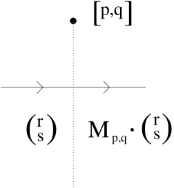
Figure 1: An $({r\atop s})$ string is shown crossing in the anti-clockwise direction the branch cut associated to a $[p,q]$ 7-brane. The outgoing string is the $M_{p,q}\cdot({r\atop s})$ string.

It is simple to show that $({p\atop q})$ is the only eigenvector of $M_{p,q}$, and that the corresponding eigenvalue is one. This is sensible for it says that only a $({p\atop q})$ string can go around a $[p,q]$ 7-brane without being changed.

2.2 Open string junctions

Let us next analyze under which conditions three string junctions are allowed. Suppose that three oriented open strings $({p_{i}\atop q_{i}})$, $i=1,2,3$ form a three string junction, where, as always, $p_{i}$ and $q_{i}$ are relatively prime. As explained in [12, 17], charge conservation implies then that the charges of the three strings must satisfy

$$\begin{array}[]{lcl}p_{1}+p_{2}+p_{3}&=&0\,,\\ q_{1}+q_{2}+q_{3}&=&0\,.\end{array}$$ (2.5)

It is however not clear whether this condition is already sufficient. In fact, one may also want to require that a junction is only allowed if one of the strings participating in the junction can end on another one, and in the following we shall also impose this condition. It is known that the fundamental string $({\pm 1\atop 0})$ can end on the D-string $({0\atop 1})$. Using the $\mbox{SL}(2,{\sf Z\!\!Z})$ transformation $\pmatrix{p&r\cr q&s}$, this then implies that a $({\pm p\atop\pm q})$ string can end on a $({r\atop s})$ string. We therefore conclude

A $({p\atop q})$ string can end on a $({r\atop s})$ string if $ps-qr=\pm 1$.

If $({\pm p\atop\pm q})$ can end on $({r\atop s})$, then it can also end on the outgoing $({p+r\atop q+s})$ string of the three string junction (whose charges are determined by (2.5)). Furthermore, the relation is symmetric: if $({p\atop q})$ can end on $({r\atop s})$, then $({r\atop s})$ can end on $({p\atop q})$. We shall therefore say that two types of strings are compatible if they can end on one another.

It was suggested in [12] that under suitable conditions on the geometry of the junction, the resulting configuration should be BPS.

Higher string junctions should also exist; for example, four-string junctions should arise when the intermediate string joining two allowed three-string junctions collapses. Similar considerations should also apply to higher string junctions. At present, we do not know if these are all the allowed $n\geq 4$ string junctions.

2.3 Brane crossings and creation of string junctions

Next we want to explain that the three-string junction arises naturally when a suitable string crosses a 7-brane. The effect is actually U-dual to the Hanany-Witten effect [10]; for the case of an D-string $({0\atop 1})$ and an D7-brane $[1,0]$ this follows from the arguments in [11]. The general case can then be deduced by $\mbox{SL}(2,Z)$ transformations.

Suppose then that an $({r\atop s})$ string is crossing the branch cut of a $[p,q]$ 7-brane on which it is not allowed to end, i.e. $(r,s)\not=\pm(p,q)$. If the $({r\atop s})$ string is compatible with the $({p\atop q})$ strings that can end on the 7-brane, i.e. if $ps-qr=e$, where $e=+1,\hbox{or}~{},-1$, an interesting possibility arises: as the $({r\atop s})$-string crosses the 7-brane, a $({p\atop q})$-string is created that joins the $({r\atop s})$ string to the 7-brane; this is represented pictorially in figure 2.

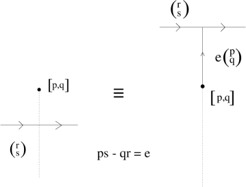
Figure 2: A 1-brane is created as the string crosses the 7-brane.

We should mention that the incoming and outgoing charges of the string are the same for both representations. This follows from the equation

$$M_{p,q}\cdot\pmatrix{r\cr s}=\pmatrix{r\cr s}+e\pmatrix{p\cr q}\,,$$ (2.6)

which in turn can be derived with the help of (2.3).

The two different representations are different descriptions of the same BPS state; as in the Hanany-Witten effect they are valid in different regions of the moduli space of positions of the 7-branes.

2.4 Mutually nonlocal 7-branes

In both the type IIB picture of compactification on $S^{2}$ and on the equivalent F-theory picture of an elliptically fibered K3 with base $S^{2}$, topological consistency conditions require a total of 24 7-branes. As the branes approach each other we get singularities that give rise to enhanced gauge symmetries.

In one familiar configuration the branes fall into four bunches of six branes each, each bunch defining a $D_{4}$ singularity of K3 and giving rise to an $so(8)$ gauge algebra [9]. The six 7-branes on each bunch can be viewed as four ordinary $[1,0]$ D7-branes, to be denoted as $A$-branes, one $[3,-1]$ 7-brane ($B$-brane), and one $[1,-1]$ 7-brane ($C$-brane)

$$A:[1,0]\,,\quad B:[3,-1]\,,\quad C:[1,-1]\,.$$ (2.7)

The corresponding monodromies, which we denote by abuse of notation as $A$, $B$ and $C$, are obtained from (2.3), and are given as

$$A=\pmatrix{1&1\cr 0&1}\,,\quad B=\pmatrix{4&9\cr-1&-2}\,,\quad C=\pmatrix{2&1\cr-1&0}\,.$$ (2.8)

Let us denote by $n_{A},n_{B},$ and $n_{C}$ the number of $A$, $B$ and $C$ branes, respectively. Then we have for $so(8)$

$$so(8):\,n_{A}=4,\quad n_{B}=1\,,\quad n_{C}=1\,.$$ (2.9)

As we encircle successively the $C$, $B$ and four $A$ branes, we obtain an effective monodromy

$$A^{4}BC=-{\mathchoice{{\rm 1\mskip-4.0mul}}{{\rm 1\mskip-4.0mul}}{{\rm 1\mskip-4.5mul}}{{\rm 1\mskip-5.0mul}}}\,.$$ (2.10)

All configurations of branes that will be relevant for us will have some number of $A$, $B$ and $C$ branes. (In fact we shall always have $n_{B}=1$.) The open strings joining the same types of branes along trivial paths generate the gauge algebra $su(n_{A})\times su(n_{C})\times u(1)$. In the following we shall mostly ignore the $u(1)$ factor which arises by some mixing of the $u(1)$ factors that are associated to the different groups of branes.

For the different singularities on K3, the corresponding configurations of (mutually non-local) 7-branes can be determined. As analyzed in [5] the branes can for example bunch into three groups of eight branes, where each bunch consist of five $A$-branes, one $B$-brane and two $C$-branes, and gives rise to the $E_{6}$ gauge algebra [6]

$$E_{6}:\,n_{A}=5,\quad n_{B}=1\,,\quad n_{C}=2\,.$$ (2.11)

As we encircle successively the two $C$ branes, the $B$ brane, and the five $A$ branes, we obtain an effective monodromy

$$A^{5}BC^{2}=\pmatrix{-1&-1\cr 1&0}=(ST)^{2},\quad\hbox{with}\quad S=\pmatrix{0&-1\cr 1&0}\,.$$ (2.12)

The monodromy $(ST)^{2}$ cubes to the identity, $[(ST)^{2}]^{3}=1$, and leaves $\tau=\exp(i\pi/3)$ invariant; we can thus chose $\tau=\exp(i\pi/3)$ as a constant coupling.

The 24 branes can also fall into one bunch of six, and two bunches of nine branes, giving rise to an $so(8)\times E_{7}\times E_{7}$ gauge algebra. One can in this way realize $E_{7}$ with nine non-local branes [6],

$$E_{7}:\,n_{A}=6,\quad n_{B}=1\,,\quad n_{C}=2\,,$$ (2.13)

and with the associated monodromy

$$A^{6}BC^{2}=S\,.$$ (2.14)

This monodromy requires a (constant) string coupling $\tau=i$ for the background.

Finally, one can group the 24 branes into a bunch of six, a bunch of eight, and a bunch of ten giving rise to an $so(8)\times E_{6}\times E_{8}$ algebra. One can thus realize $E_{8}$ with ten non-local branes [6],

$$E_{8}:\,n_{A}=7,\quad n_{B}=1\,,\quad n_{C}=2\,.$$ (2.15)

giving rise to an overall monodromy

$$A^{7}BC^{2}=TS\,.$$ (2.16)

The constant string coupling for this background is $\tau=\exp(i\pi/3)$.

2.5 Exceptional Lie-algebras and perturbative subalgebras

In this section we will consider the Lie algebras $so(8),E_{6},E_{7}$ and $E_{8}$, and we will show, for each of them, how the adjoint representation transforms under the Lie subalgebra that can be realized manifestly with the branes indicated in the previous section. The material in this section is essentially an elaboration and explanation of some of the results of Ref.[6].

We begin with the case of $so(8)$. Here the manifest subalgebra is $u(4)$ and therefore we consider $so(8)\to u(4)=su(4)\times u(1)$ where the vector of $so(8)$ decomposes as $8\to 4_{-1}+\overline{4}_{+1}$. The adjoint $28=(8\times 8)_{a}$ breaks as

$$28\to 15_{0}+1_{0}+6_{-2}+6_{+2}\,.$$ (2.17)

The Lie algebra $so(8)$ can thus be viewed as generated by the elements that generate $su(4)\times u(1)$ plus twelve other generators transforming as $6_{-2}+6_{+2}$. The Lie bracket of $6_{-2}$ with $6_{+2}$ gives both the $15_{0}$ and the $1_{0}$.

For $E_{6}$ we are interested in the subalgebra $su(5)\times su(2)\times u(1)$. This subalgebra is embedded in $E_{6}$ via the maximal regular subalgebra $su(6)\times su(2)\subset E_{6}$. For $E_{6}\to su(6)\times su(2)$ the adjoint decomposes as $78\to(35,1)+(1,3)+(20,2)$. Since for $su(6)\to su(5)\times u(1)$, we have $6\to 5_{1}+1_{-5}$, we thus find

$$78 \to \,(24,1)_{0}+(1,1)_{0}+(1,3)_{0}$$

$$+(10,2)_{-3}+(\overline{10},2)_{3}$$

$$+\,(\overline{5},1)_{-6}\,\,+\,(5,1)_{6}\,.$$

For the case of $E_{7}$ we are interested in the manifest subalgebra $su(6)\times su(2)\times u(1)$, which can be embedded into $E_{7}$ via the maximal regular subalgebras $su(8)\subset E_{7}$, $so(12)\times su(2)\subset E_{7}$ or $su(6)\times su(3)\subset E_{7}$.

The route via $su(8)$ uses the further decomposition $su(8)\to su(6)\times su(2)\times u(1)$ with $8\to(6,1)_{1}+(1,2)_{-3}$. In this decomposition, the adjoint of $E_{7}$ breaks into $su(6)\times su(2)\times u(1)$ representations which contain among others, bifundamentals $(6,2)$ and $(\overline{6},2)$. Such representations cannot be obtained with the mutually non-local branes we are considering, and therefore this embedding of the desired subalgebra is not relevant for our purposes. The embeddings of $su(6)\times su(2)\times u(1)$ in $E_{7}$ defined by using the last two maximal subalgebras give the same answer. Under $E_{7}\to so(12)\times su(2)$ we have $133\to(66,1)+(32^{\prime},2)+(1,3)$, and under $so(12)\to su(6)\times u(1)$ we have $12\to 6_{1}+6_{-1}$ and $32^{\prime}\to 1_{3}+1_{-3}$ $+15_{-1}+\overline{15}_{+1}$, and we therefore obtain

$$133 \to \,(35,1)_{0}+(1,1)_{0}+(1,3)_{0}$$

$$+(15,2)_{-1}+(\overline{15},2)_{1}$$

$$+(\overline{15},1)_{-2}+(15,1)_{2}$$

$$+\,(1,2)_{-3}\,+\,(1,2)_{3}\,.$$

Finally let us consider the case of $E_{8}$, where the manifest subalgebra is $su(7)\times su(2)\times u(1)$. This subalgebra can be embedded into $E_{8}$ via the maximal regular subalgebras $su(9)\subset E_{8}$ and $E_{7}\times su(2)\subset E_{8}$. In the first case, we obtain again bi-fundamentals which do not arise in the brane configurations we are considering. In the second case, the adjoint of $E_{8}$ decomposes as $248\to(133,1)+(1,3)+(56,2)$. We then have $E_{7}\to su(8)$ with $133\to 63+70$ and $56\to 28+\bar{2}8$, and finally $su(8)\to su(7)\times u(1)$ with $8\to 7_{1}+1_{-7}$. Using this chain of embeddings we thus find that under $E_{8}\to su(7)\times su(2)\times u(1)$ we have

$$248 \to \,(48,1)_{0}+(1,1)_{0}+(1,3)_{0}$$

$$+(21,2)_{2}+(\overline{21},2)_{-2}$$

$$+(\overline{35},1)_{4}+(35,1)_{-4}$$

$$+(\overline{7},2)_{6}+(\overline{7},2)_{-6}$$

$$+(7,1)_{8}+(\overline{7},1)_{-8}\,.$$

This information can be conveniently organized in the following table. The first column contains the manifestly realized subalgebra, and the other columns describe the representations of the additional generators. These are either in the fundamental (2nd and 4th column) or the singlet (3rd and 5th column) of the $su(2)$ algebra. The representation of $su(n_{A})$ is the completely antisymmetric 2nd, 4th, 6th rank tensor and the fundamental, respectively. In the top line, the representations are labeled by boxes which are reminiscent of the Young tableaux of $su(n)\times su(2)$, and we shall often use this notation below.

  Manifest subalgebra $$(\mathchoice{\vbox{\vbox{\hrule height=0.6pt\hbox{\vrule width=0.6pt,height=5.0pt\kern 5.0pt\vrule width=0.6pt} \hrule height=0.6pt}}}{\vbox{\vbox{\hrule height=0.6pt\hbox{\vrule width=0.6pt,height=5.0pt\kern 5.0pt\vrule width=0.6pt} \hrule height=0.6pt}}}{\vbox{\vbox{\hrule height=0.4pt\hbox{\vrule width=0.4pt,height=2.7pt\kern 2.7pt\vrule width=0.4pt} \hrule height=0.4pt}}}{\vbox{\vbox{\hrule height=0.4pt\hbox{\vrule width=0.4pt,height=1.9pt\kern 1.9pt\vrule width=0.4pt} \hrule height=0.4pt}}}^{2}_{a},\mathchoice{\vbox{\vbox{\hrule height=0.6pt\hbox{\vrule width=0.6pt,height=5.0pt\kern 5.0pt\vrule width=0.6pt} \hrule height=0.6pt}}}{\vbox{\vbox{\hrule height=0.6pt\hbox{\vrule width=0.6pt,height=5.0pt\kern 5.0pt\vrule width=0.6pt} \hrule height=0.6pt}}}{\vbox{\vbox{\hrule height=0.4pt\hbox{\vrule width=0.4pt,height=2.7pt\kern 2.7pt\vrule width=0.4pt} \hrule height=0.4pt}}}{\vbox{\vbox{\hrule height=0.4pt\hbox{\vrule width=0.4pt,height=1.9pt\kern 1.9pt\vrule width=0.4pt} \hrule height=0.4pt}}}) (\mathchoice{\vbox{\vbox{\hrule height=0.6pt\hbox{\vrule width=0.6pt,height=5.0pt\kern 5.0pt\vrule width=0.6pt} \hrule height=0.6pt}}}{\vbox{\vbox{\hrule height=0.6pt\hbox{\vrule width=0.6pt,height=5.0pt\kern 5.0pt\vrule width=0.6pt} \hrule height=0.6pt}}}{\vbox{\vbox{\hrule height=0.4pt\hbox{\vrule width=0.4pt,height=2.7pt\kern 2.7pt\vrule width=0.4pt} \hrule height=0.4pt}}}{\vbox{\vbox{\hrule height=0.4pt\hbox{\vrule width=0.4pt,height=1.9pt\kern 1.9pt\vrule width=0.4pt} \hrule height=0.4pt}}}^{4}_{a},\cdot) (\mathchoice{\vbox{\vbox{\hrule height=0.6pt\hbox{\vrule width=0.6pt,height=5.0pt\kern 5.0pt\vrule width=0.6pt} \hrule height=0.6pt}}}{\vbox{\vbox{\hrule height=0.6pt\hbox{\vrule width=0.6pt,height=5.0pt\kern 5.0pt\vrule width=0.6pt} \hrule height=0.6pt}}}{\vbox{\vbox{\hrule height=0.4pt\hbox{\vrule width=0.4pt,height=2.7pt\kern 2.7pt\vrule width=0.4pt} \hrule height=0.4pt}}}{\vbox{\vbox{\hrule height=0.4pt\hbox{\vrule width=0.4pt,height=1.9pt\kern 1.9pt\vrule width=0.4pt} \hrule height=0.4pt}}}^{6}_{a},\mathchoice{\vbox{\vbox{\hrule height=0.6pt\hbox{\vrule width=0.6pt,height=5.0pt\kern 5.0pt\vrule width=0.6pt} \hrule height=0.6pt}}}{\vbox{\vbox{\hrule height=0.6pt\hbox{\vrule width=0.6pt,height=5.0pt\kern 5.0pt\vrule width=0.6pt} \hrule height=0.6pt}}}{\vbox{\vbox{\hrule height=0.4pt\hbox{\vrule width=0.4pt,height=2.7pt\kern 2.7pt\vrule width=0.4pt} \hrule height=0.4pt}}}{\vbox{\vbox{\hrule height=0.4pt\hbox{\vrule width=0.4pt,height=1.9pt\kern 1.9pt\vrule width=0.4pt} \hrule height=0.4pt}}}) (\mathchoice{\vbox{\vbox{\hrule height=0.6pt\hbox{\vrule width=0.6pt,height=5.0pt\kern 5.0pt\vrule width=0.6pt} \hrule height=0.6pt}}}{\vbox{\vbox{\hrule height=0.6pt\hbox{\vrule width=0.6pt,height=5.0pt\kern 5.0pt\vrule width=0.6pt} \hrule height=0.6pt}}}{\vbox{\vbox{\hrule height=0.4pt\hbox{\vrule width=0.4pt,height=2.7pt\kern 2.7pt\vrule width=0.4pt} \hrule height=0.4pt}}}{\vbox{\vbox{\hrule height=0.4pt\hbox{\vrule width=0.4pt,height=1.9pt\kern 1.9pt\vrule width=0.4pt} \hrule height=0.4pt}}},\cdot) E_{6} su(5)\times su(2)\times u(1) (10,2)_{-3} (\overline{5},1)_{-6} -- -- E_{7} {su(6)\times su(2)\times u(1)} (15,2)_{-1} (\overline{15},1)_{-2} (1,2)_{-3} -- E_{8} {su(7)\times su(2)\times u(1)} (21,2)_{2} (\overline{35},1)_{4} (\overline{7},2)_{6} (7,1)_{8}$$

3 Geodesics and BPS states

In the IIB superstring approach to exceptional gauge groups of Ref.[6], the gauge vectors arise as geodesics on the compactifying two-sphere whose endpoints are 7-branes. The property of the different paths to be geodesics is somewhat difficult to analyze, and it was only checked numerically in [6].

In this section we shall take some small steps that improve this situation. We will be able to show on general grounds that certain classes of geodesics, for specific regions of the moduli of positions of the 7-branes, exist. However, not even these (simple) classes of geodesics seem to exist for completely arbitrary positions of the 7-branes. This is in accord with our proposal that the conventional open strings do not represent the relevant BPS states throughout the whole moduli spaces of positions of the 7-branes. Rather, there exist various regions of the moduli space where the relevant BPS states correspond to multi-pronged strings.

From the F-theory point of view, the ordinary open string geodesics correspond to two-spheres with two marked points (which are the locations of the 7-branes, where the torus degenerates). Our $n$-pronged open string configurations are the natural generalization to two-spheres with $n$ marked points; the locations of the open string junctions themselves do not represent degenerate tori. Similar configurations have also been considered before in a slightly different context in Ref. [18].

3.1 Metrics on the two-sphere

The geodesics that we aim to understand are geodesics on a two-sphere with a special metric. This metric was first obtained in [19], and it is best described by using the F-theory picture of an elliptically fibered K3 whose base is the $S^{2}$ in question. Taking $z$ to be the complex coordinate on $S^{2}$, the K3 is described by the equation

$$y^{2}=x^{3}+f(z)x+g(z)\,,$$ (3.1)

which defines a torus with a complex structure for each value of $z$. Here $f$ and $g$ are polynomials of degree eight and twelve, respectively, and the complex structure of the torus $\tau(z)$ is implicitly defined by the equation

$$j(\tau(z))=4\cdot(24f)^{3}/\Delta\,,\quad\hbox{with}\quad\Delta\equiv 27g^{2}+4f^{3}=\prod_{i=1}^{24}(z-z_{i})\,,$$ (3.2)

where the $z_{i}$’s are the positions of the 7-branes in the IIB description. Properly speaking, $\tau(z)$ is not a function, but defines a holomorphic section in an $\mbox{SL}(2,{\sf Z\!\!Z})$ bundle over the two-sphere.

The metric on the $S^{2}$ is then given as

$$ds^{2}=\tau_{2}\,\eta(\tau)^{2}\bar{\eta}(\bar{\tau})^{2}\prod_{i}(z-z_{i})^{-1/12}(\bar{z}-\bar{z}_{i})^{-1/12}\,dzd\bar{z}\,,$$ (3.3)

where $\tau_{2}=\mbox{Im}(\tau)$, and

$$\eta^{2}(\tau)=q^{1/12}\prod_{n=1}^{\infty}(1-q^{n})^{2}\,,\quad q=\exp(2\pi i\tau)\,,$$ (3.4)

is the square of the Dedekind eta-function which satisfies

$$\eta^{2}(-1/\tau)=-i\tau\eta^{2}(\tau)\,,\quad\eta^{2}(\tau+1)=e^{i\pi/6}\,\eta^{2}(\tau)\,.$$ (3.5)

It is straightforward to show that this metric is invariant under $\mbox{SL}(2,{\sf Z\!\!Z})$ transformations of $\tau$. The masses of the states associated to $({p\atop q})$ strings must also take into account the string tension $T_{p,q}$ of the $({p\atop q})$ string [20],

$$T_{p,q}={1\over\sqrt{\tau_{2}}}\,|p-q\tau\,|\,.$$ (3.6)

It is then natural to introduce the length element $ds_{p,q}=T_{p,q}ds$ which measures correctly the mass of the corresponding string, and the corresponding effective metric $ds^{2}_{p,q}$

$$ds_{p,q}^{2}=h(z)_{p,q}\,\overline{h_{p,q}(z)}\,dzd\bar{z}\,,\quad\hbox{with}\quad h_{p,q}(z)=(p-q\tau)\,\eta^{2}(\tau)\prod_{i}(z-z_{i})^{-1/12}\,.$$ (3.7)

Under an SL(2,Z) transformation we have

$$\tau\to\tau^{\prime}={a\tau+b\over c\tau+d}\,,\quad\pmatrix{p\cr q}\to\pmatrix{p^{\prime}\cr q^{\prime}}=\pmatrix{a&b\cr c&d}\cdot\pmatrix{p\cr q}\,,\,\,\,\hbox{and}\quad T_{p,q}\to T_{p^{\prime},q^{\prime}}\,,$$ (3.8)

and it follows that the effective metric is continuous across the branch cuts emerging from the 7-branes, i.e. $ds_{p,q}(\tau)=ds_{p^{\prime}q^{\prime}}(\tau^{\prime})$. Since the effective metric is the modulus of an analytic one-form, it is flat, except for possible singularities.

The metric (3.7) is typically rather complicated, but in some cases the metric behaves (at least at large distance) as if it had a conical singularity. By this one means that $h_{p,q}(z)$ is of the form

$$h_{p,q}(z)=z^{-{\theta\over 2\pi}}(c+c^{\prime}z+\cdots)\,,$$ (3.9)

where $\theta$ is the defect angle, and we have assumed, for simplicity, that the conical singularity is at $z=0$. Here the expression in parenthesis is simply the expansion of an analytic function that is regular at the origin. In particular, the metric (3.7) is of this form if the term $(p-q\tau)\eta^{2}(\tau)$ is a constant (as a function of $z$), and all 7-branes are located at $z_{i}=0$.

To proceed let us consider the configuration of a fundamental string in the vicinity of a $[1,0]$ D7-brane, which, for convenience we place at $z=0$. Since $M_{1,0}=T$, we have

$$\tau(z)\sim{1\over 2\pi i}\ln z\,.$$ (3.10)

and therefore $\eta^{2}\sim z^{1\over 12}$. It then follows that the factor $h_{1,0}(z)\sim\eta^{2}z^{-{1\over 12}}$ is regular in this situation, and the $({1\atop 0})$ string does not see a metric singularity at the position of the $[1,0]$ D7-brane. This is, of course, as expected.

We can next consider the case where a $({1\atop 0})$ string loops around a collection of $N$ branes located in the vicinity of $z=0$. The metric (3.7), far away from $z=0$ reads then

$$h_{1,0}\sim\eta^{2}(z)z^{-{N\over 12}}\,.$$ (3.11)

If the collection of $N$ branes create an effective monodromy matrix

$$M=\pmatrix{-1&\,l\cr 0&-1}\,,$$ (3.12)

we have, as we go (anti-clockwise) around these branes, $\tau\to\tau-l$, and therefore

$$\tau(z)\sim{-l\over 2\pi i}\ln z\,,\quad\quad\eta^{2}(\tau(z))\sim z^{-{l\over 12}}\,.$$ (3.13)

This implies that $h_{1,0}\sim z^{-{(N+l)\over 12}}$, and the group of $N$ branes creates a conical singularity that corresponds to a deficit angle of $(N+l)2\pi/12$.

3.2 Indirect $AA$ and $CC$ geodesics

The above considerations can be used to discuss the nature of $AA$ and $CC$ geodesics that encircle some number of 7-branes. As we shall see, in suitable limits we can describe both kinds of geodesics as geodesics on a cone with defect angle $\pi$. This is effectively an orientifold description.

Let us first consider the case of $AA$ geodesics. The different (potential) geodesics that begin and end on an $A$ brane fall into two classes, the direct and the indirect paths. The former are all paths which do not cut any branch cuts, and the indirect paths are those which begin on $A$, go around a $C$ brane, a $B$ brane, and then end again on an $A$ brane. These geodesics are for example relevant for the brane configuration of $so(8)$ which requires four $A$ branes, one $B$ brane and one $C$ brane. In this case, if all six branes coincide in a point, (2.10) implies that the effective monodromy of the complete configuration is minus the identity matrix. In the notation of (3.12) we then have $l=0$ and the metric for the fundamental string has a conical singularity with defect angle $\pi$.

As we remove the $A$ branes from the collapsed configuration the defect angle for the $ds_{1,0}$ metric does not change. This follows for example from the fact that an $A$ brane does not represent any singularity for the fundamental $({1\atop 0})$ string. We can also check this explicitly, as $BC$ is of the form (3.12) with $l=4$, and thus $N+l=2+4=6$ giving again the defect angle of $\pi$.

The situation for $CC$ strings is similar. Again there exist the direct paths, and the indirect paths encircle four $A$ branes and one $B$ brane, whose effective monodromy is $A^{4}B=\pmatrix{0&1\cr-1&-2}$. It is convenient to perform an $\mbox{SL}(2,{\sf Z\!\!Z})$ transformation $g=\pmatrix{1&0\cr-1&1}$ which turns the $C$-brane into a conventional $[1,0]$ D7-brane. The effective monodromy of the group of five 7-branes is then $g^{-1}(A^{4}B)g=\pmatrix{-1&1\cr 0&-1}$, which is of the form (3.12) with $l=1$. Altogether we therefore have again a conical singularity with a defect angle of $\pi$ (as $N+l=5+1=6$).

The geometry of geodesics in a cone of defect angle $\pi$ is simple to understand. Between any two branes located away from the apex there are two geodesics, one ‘direct’ geodesic which would become trivial should the branes approach each other, and the ‘indirect’ geodesic which goes around the other side of the cone. As long as the two $A$ branes are not contained on the same radial line away from the apex, both geodesics avoid the apex. On the other hand, the indirect geodesics going from a brane to itself will necessarily go through the apex, and their existence is therefore questionable. This suggests that for $n$ branes in the vicinity of a cone of defect angle $\pi$, we get $n^{2}$ direct geodesics (distinguishing orientation) and $n(n-1)$ indirect geodesics.

This analysis applies directly only to the situation, where for the $AA$ strings, $B$ and $C$ coincide (and for the $CC$ string, the four $A$s and $B$ coincide). If we separate $B$ and $C$, then the above picture is only approximately true whenever we are far away from the region around the apex. In the regions of moduli space where this approximation is not valid, some of the geodesics are likely to become questionable, and it seems plausible that open string junctions become the relevant objects.

4 Exceptional groups

In this section we shall analyze the various different geodesics (and their representatives involving string junctions) which are relevant for the description of the exceptional groups. As mentioned earlier, the direct geodesics between the $A$ branes and between the $C$ branes account for the “manifest” gauge subgroup. Here we shall only consider the additional generators. We shall demonstrate that these generators have the correct charges, and that they multiply correctly in order to account for the structure of the exceptional groups.

4.1 Versions of indirect $AA$ strings

We shall start by considering the indirect $AA$ strings in more detail. As explained before, these geodesics start on an $A$ brane, encircle a $C$ brane and a $B$ brane anti-clockwise, and end on a different $A$ brane; this is shown in Fig. 3 (a). From now on we shall always use the convention that heavy dots represent $A$ branes, small circles represent $B$ branes, and small squares represent $C$ branes. The dotted lines that emanate from the 7-brane represent the corresponding branch cut, and the strings that begin or end at a $[p,q]$ 7-brane are always $({p\atop q})$ strings.

The configuration in Fig. 3 (a) is allowed as the monodromy of $C$ and $B$ transforms the $({1\atop 0})$ string that starts at the right $A$ brane into a $BC\cdot({1\atop 0})=({-1\atop 0})$ string that arrives at the left $A$ brane; this is equivalent to a $({1\atop 0})$ string departing from the left $A$ brane. We note that both $A$ branes have departing $({1\atop 0})$ strings.

As explained in the previous section, only those paths are geodesics, for which the string begins and ends on different $A$ branes. This can now also be understood pictorially: we can compose the strings in Fig. 3 (a) with ‘direct’ $AA$ strings (which represent the gauge bosons of $su(n_{A})$), and the fact that the string in Fig. 3 (a) departs from both $A$ branes implies that the different strings transform as the antisymmetric tensor representation of $su(n_{A})$.

On the other hand, for fixed $A$ endpoints, there exist $n_{C}$ different such configurations, depending on which $C$ brane is encircled. One should expect that the indirect $AA$ strings transform in the fundamental representation of $su(n_{C})$ (which is generated by the direct $CC$ strings), but since the configurations of Fig. 3 (a) do not have any endpoints on a $C$ brane this is not manifest.

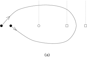
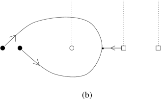
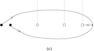
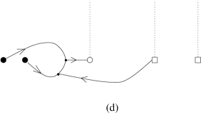
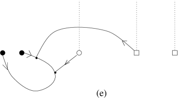
Figure 3: Five versions of the $AA$ geodesic which transforms as $(\mathchoice{\vbox{\vbox{\hrule height=0.6pt\hbox{\vrule width=0.6pt,height=5.0pt\kern 5.0pt\vrule width=0.6pt} \hrule height=0.6pt}}}{\vbox{\vbox{\hrule height=0.6pt\hbox{\vrule width=0.6pt,height=5.0pt\kern 5.0pt\vrule width=0.6pt} \hrule height=0.6pt}}}{\vbox{\vbox{\hrule height=0.4pt\hbox{\vrule width=0.4pt,height=2.7pt\kern 2.7pt\vrule width=0.4pt} \hrule height=0.4pt}}}{\vbox{\vbox{\hrule height=0.4pt\hbox{\vrule width=0.4pt,height=1.9pt\kern 1.9pt\vrule width=0.4pt} \hrule height=0.4pt}}}^{2}_{a},\mathchoice{\vbox{\vbox{\hrule height=0.6pt\hbox{\vrule width=0.6pt,height=5.0pt\kern 5.0pt\vrule width=0.6pt} \hrule height=0.6pt}}}{\vbox{\vbox{\hrule height=0.6pt\hbox{\vrule width=0.6pt,height=5.0pt\kern 5.0pt\vrule width=0.6pt} \hrule height=0.6pt}}}{\vbox{\vbox{\hrule height=0.4pt\hbox{\vrule width=0.4pt,height=2.7pt\kern 2.7pt\vrule width=0.4pt} \hrule height=0.4pt}}}{\vbox{\vbox{\hrule height=0.4pt\hbox{\vrule width=0.4pt,height=1.9pt\kern 1.9pt\vrule width=0.4pt} \hrule height=0.4pt}}})$ of $su(n_{A})\times su(n_{C})$.

We can now, however, change the presentation by letting the open string cross the $C$ brane it encloses. This is allowed by the rule described in Fig. 2 as the $({0\atop 1})$ string is compatible with the $({1\atop-1})$ string associated to a $C$ brane. After crossing we get the extra open string prong emerging from the $C$ brane, and we have obtained a three-string junction as a representation of the BPS state; this is illustrated in Fig. 3 (b). In this presentation the fact that the states transform as fundamentals of $su(n_{C})$ is now manifest, as we have an open string ending on the $C$ brane, and the states compose naturally with direct $CC$ strings.

Additional presentations are possible by doing further moves. We can go from (a) to (c) by pushing the open string across the $C$ brane that is not enclosed; this leads to a diagram where the prong goes into the $C$ brane. Two more presentations that are useful are shown in (d) and (e), both of which follow by crossing the $B$ brane in presentation (b).

The complex conjugate representation is described by exactly the same diagrams with the exception that the arrows are reversed. Thus, for example, while Fig. 3 (a) represents the $(10,2)_{-3}$ for the case of $E_{6}$, the same figure with the $({1\atop 0})$ strings going into the $A$ branes would represent the $(\overline{10},2)_{3}$. This is sensible on various accounts. First and foremost, the diagrams with arrows reversed are consistent if the original representations are consistent: reversal of arrows is compatible with charge conservation at junctions and with the crossing of branch cuts. By construction they represent the same number of states as the original representation, and finally we can combine a representation with its complex conjugate by gluing the string prongs at all 7-branes to obtain a singlet.

4.2 Versions of the $CC$ strings

As can be seen from the table given in section 2, the non-manifest generators of $E_{6}$ include the $AA$ states considered above and transforming as $(\mathchoice{\vbox{\vbox{\hrule height=0.6pt\hbox{\vrule width=0.6pt,height=5.0pt\kern 5.0pt\vrule width=0.6pt} \hrule height=0.6pt}}}{\vbox{\vbox{\hrule height=0.6pt\hbox{\vrule width=0.6pt,height=5.0pt\kern 5.0pt\vrule width=0.6pt} \hrule height=0.6pt}}}{\vbox{\vbox{\hrule height=0.4pt\hbox{\vrule width=0.4pt,height=2.7pt\kern 2.7pt\vrule width=0.4pt} \hrule height=0.4pt}}}{\vbox{\vbox{\hrule height=0.4pt\hbox{\vrule width=0.4pt,height=1.9pt\kern 1.9pt\vrule width=0.4pt} \hrule height=0.4pt}}}^{2}_{a},\mathchoice{\vbox{\vbox{\hrule height=0.6pt\hbox{\vrule width=0.6pt,height=5.0pt\kern 5.0pt\vrule width=0.6pt} \hrule height=0.6pt}}}{\vbox{\vbox{\hrule height=0.6pt\hbox{\vrule width=0.6pt,height=5.0pt\kern 5.0pt\vrule width=0.6pt} \hrule height=0.6pt}}}{\vbox{\vbox{\hrule height=0.4pt\hbox{\vrule width=0.4pt,height=2.7pt\kern 2.7pt\vrule width=0.4pt} \hrule height=0.4pt}}}{\vbox{\vbox{\hrule height=0.4pt\hbox{\vrule width=0.4pt,height=1.9pt\kern 1.9pt\vrule width=0.4pt} \hrule height=0.4pt}}})$ of $su(5)\times su(2)$, and, in addition, states transforming as $(\mathchoice{\vbox{\vbox{\hrule height=0.6pt\hbox{\vrule width=0.6pt,height=5.0pt\kern 5.0pt\vrule width=0.6pt} \hrule height=0.6pt}}}{\vbox{\vbox{\hrule height=0.6pt\hbox{\vrule width=0.6pt,height=5.0pt\kern 5.0pt\vrule width=0.6pt} \hrule height=0.6pt}}}{\vbox{\vbox{\hrule height=0.4pt\hbox{\vrule width=0.4pt,height=2.7pt\kern 2.7pt\vrule width=0.4pt} \hrule height=0.4pt}}}{\vbox{\vbox{\hrule height=0.4pt\hbox{\vrule width=0.4pt,height=1.9pt\kern 1.9pt\vrule width=0.4pt} \hrule height=0.4pt}}}^{4}_{a},\cdot)$. These are states that can be represented as open strings beginning and ending on $C$ branes, and enclosing four $A$ branes and one $B$ brane [6]; this geodesic is shown in Fig. 4 (a). A $({1\atop-1})$ string crosses a $B$ brane and four $A$ branes and in this process becomes a $A^{4}B\cdot({1\atop-1})=({-1\atop+1})$ string ending on the other $C$ brane, or equivalently, an $({1\atop-1})$ departing from it. As explained before in section 3, only those states are BPS which begin and end on two different $C$ branes. This is also consistent with the fact that the states in Fig. 4 (a) transform as the antisymmetric representation of $su(n_{C})$. As $n_{C}=2$ for the cases of $E_{6}$, $E_{7}$ and $E_{8}$, the indirect $CC$ strings will be singlets of $su(2)$.

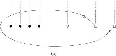
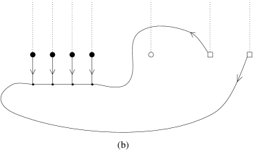
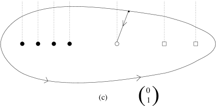
Figure 4: Different versions of the indirect $CC$ geodesic which transforms as $(\mathchoice{\vbox{\vbox{\hrule height=0.6pt\hbox{\vrule width=0.6pt,height=5.0pt\kern 5.0pt\vrule width=0.6pt} \hrule height=0.6pt}}}{\vbox{\vbox{\hrule height=0.6pt\hbox{\vrule width=0.6pt,height=5.0pt\kern 5.0pt\vrule width=0.6pt} \hrule height=0.6pt}}}{\vbox{\vbox{\hrule height=0.4pt\hbox{\vrule width=0.4pt,height=2.7pt\kern 2.7pt\vrule width=0.4pt} \hrule height=0.4pt}}}{\vbox{\vbox{\hrule height=0.4pt\hbox{\vrule width=0.4pt,height=1.9pt\kern 1.9pt\vrule width=0.4pt} \hrule height=0.4pt}}}^{4}_{a},\cdot)$ of $su(n_{A})\times su(n_{C})$.

The charge with respect to the $A$ branes can be made manifest by pushing the open string across the $A$ branes, thereby creating four open string prongs (Fig. 4(b)). The four prongs have the same direction and represent the antisymmetric part of the fourth power of the fundamental as can be seen by composing these configurations with direct $AA$ strings.

In part (c) of figure 4 we illustrate a somewhat surprising presentation of the indirect $CC$ states, where a single open string prong attaches the $B$ brane to a closed string loop by means of a three string junction. The fact that this is an allowed diagram follows, algebraically, from the fact that $({0\atop 1})$ is left invariant by $A^{4}B^{2}C^{2}$. In figure 5 we show a couple of steps that demonstrate that this representation can be related by our moves to Fig. 4 (a): as a first step we move the string in Fig. 4 (c) across the two $C$ branes thus creating two prongs. The point where the left prong joins the closed sting can be slided all the way until it stands to the left of the $A$ cuts. At this stage the upper part of the closed string can be pushed down across the $B$ brane, thereby eliminating the $B$ prong, and across the $A$ branes without creating prongs. After these steps the string looks like that in Fig. 5(b). The loop can be collapsed and we recover the familiar indirect $CC$ geodesic of Fig. 4(a).

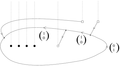
Figure 5: The left figure is a modified version of Fig. 4 (c). A couple of moves relates it to the right figure which is recognized as equivalent to Fig. 4 (a).

4.3 Construction of $E_{6}$

In the previous section we have discussed the relevant multi-pronged open strings that give rise to the representations $(10,2)_{-3}$ and $(\overline{5},1)_{-6}$ that together with their complex conjugates are necessary to enlarge the manifest subalgebra $su(5)\times su(2)\times u(1)$ to $E_{6}$. In this section we verify, using the various representatives we have discussed, that the multi-pronged open strings can be combined by the usual rules of joining open strings to give representatives in the class of the expected product. We will not discuss all possible products we may form, but rather illustrate how the rules work by means of two non-trivial examples. We should also mention that whilst we are able to generate all necessary generators, it is less clear why these are all generators, and why other (seemingly possible) diagrams are not relevant. This is presumably a difficult problem whose solution would require a better understanding of the BPS condition in this context. On the other hand, this problem is not really new: for example in the above description of $so(8)$, the $AA$ geodesic that winds twice around the $BC$ singularity does not correspond to a gauge vector, and further “selection rules” are necessary.

In the first example we discuss the product $(10,2)_{-3}\times(\overline{10},2)_{+3}$, i.e. the multiplication of $(\mathchoice{\vbox{\vbox{\hrule height=0.6pt\hbox{\vrule width=0.6pt,height=5.0pt\kern 5.0pt\vrule width=0.6pt} \hrule height=0.6pt}}}{\vbox{\vbox{\hrule height=0.6pt\hbox{\vrule width=0.6pt,height=5.0pt\kern 5.0pt\vrule width=0.6pt} \hrule height=0.6pt}}}{\vbox{\vbox{\hrule height=0.4pt\hbox{\vrule width=0.4pt,height=2.7pt\kern 2.7pt\vrule width=0.4pt} \hrule height=0.4pt}}}{\vbox{\vbox{\hrule height=0.4pt\hbox{\vrule width=0.4pt,height=1.9pt\kern 1.9pt\vrule width=0.4pt} \hrule height=0.4pt}}}^{2}_{a},\mathchoice{\vbox{\vbox{\hrule height=0.6pt\hbox{\vrule width=0.6pt,height=5.0pt\kern 5.0pt\vrule width=0.6pt} \hrule height=0.6pt}}}{\vbox{\vbox{\hrule height=0.6pt\hbox{\vrule width=0.6pt,height=5.0pt\kern 5.0pt\vrule width=0.6pt} \hrule height=0.6pt}}}{\vbox{\vbox{\hrule height=0.4pt\hbox{\vrule width=0.4pt,height=2.7pt\kern 2.7pt\vrule width=0.4pt} \hrule height=0.4pt}}}{\vbox{\vbox{\hrule height=0.4pt\hbox{\vrule width=0.4pt,height=1.9pt\kern 1.9pt\vrule width=0.4pt} \hrule height=0.4pt}}})$ with its conjugate; this is done in Fig. 6. As a first step we release the strings from the common $A$ brane and collapse it partially by crossing a $C$ brane and creating a prong. This gives Fig. 6 (b). We then move the string across the second $C$ brane, create a second prong, and obtain Fig. 6 (c). The junctions joining each of the $C$ prongs to the other string can be collapsed, and a direct open string joining the two $C$ branes can be separated out. The final result is a direct $AA$ string and a direct $CC$ string, and represents the fact that the product contains both the $(\hbox{Adj},\cdot)$ and the $(\cdot,\hbox{Adj})$ of $su(n_{A})\times su(n_{C})$.

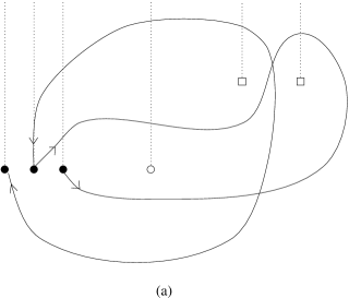
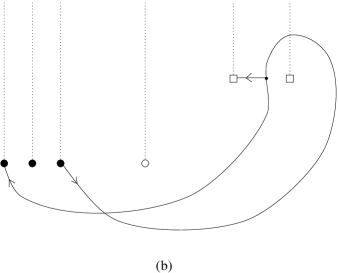
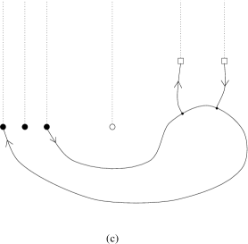
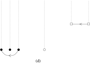
Figure 6: Multiplication of $(\mathchoice{\vbox{\vbox{\hrule height=0.6pt\hbox{\vrule width=0.6pt,height=5.0pt\kern 5.0pt\vrule width=0.6pt} \hrule height=0.6pt}}}{\vbox{\vbox{\hrule height=0.6pt\hbox{\vrule width=0.6pt,height=5.0pt\kern 5.0pt\vrule width=0.6pt} \hrule height=0.6pt}}}{\vbox{\vbox{\hrule height=0.4pt\hbox{\vrule width=0.4pt,height=2.7pt\kern 2.7pt\vrule width=0.4pt} \hrule height=0.4pt}}}{\vbox{\vbox{\hrule height=0.4pt\hbox{\vrule width=0.4pt,height=1.9pt\kern 1.9pt\vrule width=0.4pt} \hrule height=0.4pt}}}^{2}_{a},\mathchoice{\vbox{\vbox{\hrule height=0.6pt\hbox{\vrule width=0.6pt,height=5.0pt\kern 5.0pt\vrule width=0.6pt} \hrule height=0.6pt}}}{\vbox{\vbox{\hrule height=0.6pt\hbox{\vrule width=0.6pt,height=5.0pt\kern 5.0pt\vrule width=0.6pt} \hrule height=0.6pt}}}{\vbox{\vbox{\hrule height=0.4pt\hbox{\vrule width=0.4pt,height=2.7pt\kern 2.7pt\vrule width=0.4pt} \hrule height=0.4pt}}}{\vbox{\vbox{\hrule height=0.4pt\hbox{\vrule width=0.4pt,height=1.9pt\kern 1.9pt\vrule width=0.4pt} \hrule height=0.4pt}}})$ times its conjugate. The final result gives two representations, the $(\hbox{Adj},\cdot)$ and the $(\cdot,\hbox{Adj})$ of $su(n_{A})\times su(n_{C})$.

In the second example we discuss the product $(10,2)_{-3}\times({10},2)_{-3}$, i.e. the product of $(\mathchoice{\vbox{\vbox{\hrule height=0.6pt\hbox{\vrule width=0.6pt,height=5.0pt\kern 5.0pt\vrule width=0.6pt} \hrule height=0.6pt}}}{\vbox{\vbox{\hrule height=0.6pt\hbox{\vrule width=0.6pt,height=5.0pt\kern 5.0pt\vrule width=0.6pt} \hrule height=0.6pt}}}{\vbox{\vbox{\hrule height=0.4pt\hbox{\vrule width=0.4pt,height=2.7pt\kern 2.7pt\vrule width=0.4pt} \hrule height=0.4pt}}}{\vbox{\vbox{\hrule height=0.4pt\hbox{\vrule width=0.4pt,height=1.9pt\kern 1.9pt\vrule width=0.4pt} \hrule height=0.4pt}}}^{2}_{a},\mathchoice{\vbox{\vbox{\hrule height=0.6pt\hbox{\vrule width=0.6pt,height=5.0pt\kern 5.0pt\vrule width=0.6pt} \hrule height=0.6pt}}}{\vbox{\vbox{\hrule height=0.6pt\hbox{\vrule width=0.6pt,height=5.0pt\kern 5.0pt\vrule width=0.6pt} \hrule height=0.6pt}}}{\vbox{\vbox{\hrule height=0.4pt\hbox{\vrule width=0.4pt,height=2.7pt\kern 2.7pt\vrule width=0.4pt} \hrule height=0.4pt}}}{\vbox{\vbox{\hrule height=0.4pt\hbox{\vrule width=0.4pt,height=1.9pt\kern 1.9pt\vrule width=0.4pt} \hrule height=0.4pt}}})$ with itself. It is convenient to choose representatives carefully to facilitate the computation, and we use representatives (d) and (e) of Fig. 3, as is shown in Fig. 7. The prongs ending on the $B$ brane can be combined and released, and the result is immediately recognized as the $(\mathchoice{\vbox{\vbox{\hrule height=0.6pt\hbox{\vrule width=0.6pt,height=5.0pt\kern 5.0pt\vrule width=0.6pt} \hrule height=0.6pt}}}{\vbox{\vbox{\hrule height=0.6pt\hbox{\vrule width=0.6pt,height=5.0pt\kern 5.0pt\vrule width=0.6pt} \hrule height=0.6pt}}}{\vbox{\vbox{\hrule height=0.4pt\hbox{\vrule width=0.4pt,height=2.7pt\kern 2.7pt\vrule width=0.4pt} \hrule height=0.4pt}}}{\vbox{\vbox{\hrule height=0.4pt\hbox{\vrule width=0.4pt,height=1.9pt\kern 1.9pt\vrule width=0.4pt} \hrule height=0.4pt}}}^{4}_{a},\cdot)$ string in the representation shown in Fig. 4 (b). This, of course, is as it should be.

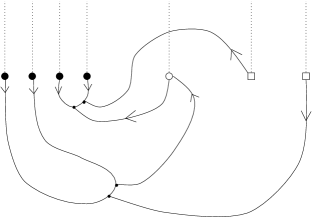
Figure 7: Multiplication of $(\mathchoice{\vbox{\vbox{\hrule height=0.6pt\hbox{\vrule width=0.6pt,height=5.0pt\kern 5.0pt\vrule width=0.6pt} \hrule height=0.6pt}}}{\vbox{\vbox{\hrule height=0.6pt\hbox{\vrule width=0.6pt,height=5.0pt\kern 5.0pt\vrule width=0.6pt} \hrule height=0.6pt}}}{\vbox{\vbox{\hrule height=0.4pt\hbox{\vrule width=0.4pt,height=2.7pt\kern 2.7pt\vrule width=0.4pt} \hrule height=0.4pt}}}{\vbox{\vbox{\hrule height=0.4pt\hbox{\vrule width=0.4pt,height=1.9pt\kern 1.9pt\vrule width=0.4pt} \hrule height=0.4pt}}}^{2}_{a},\mathchoice{\vbox{\vbox{\hrule height=0.6pt\hbox{\vrule width=0.6pt,height=5.0pt\kern 5.0pt\vrule width=0.6pt} \hrule height=0.6pt}}}{\vbox{\vbox{\hrule height=0.6pt\hbox{\vrule width=0.6pt,height=5.0pt\kern 5.0pt\vrule width=0.6pt} \hrule height=0.6pt}}}{\vbox{\vbox{\hrule height=0.4pt\hbox{\vrule width=0.4pt,height=2.7pt\kern 2.7pt\vrule width=0.4pt} \hrule height=0.4pt}}}{\vbox{\vbox{\hrule height=0.4pt\hbox{\vrule width=0.4pt,height=1.9pt\kern 1.9pt\vrule width=0.4pt} \hrule height=0.4pt}}})$ of $su(n_{A})\times su(n_{C})$ with itself. The result gives the $(\mathchoice{\vbox{\vbox{\hrule height=0.6pt\hbox{\vrule width=0.6pt,height=5.0pt\kern 5.0pt\vrule width=0.6pt} \hrule height=0.6pt}}}{\vbox{\vbox{\hrule height=0.6pt\hbox{\vrule width=0.6pt,height=5.0pt\kern 5.0pt\vrule width=0.6pt} \hrule height=0.6pt}}}{\vbox{\vbox{\hrule height=0.4pt\hbox{\vrule width=0.4pt,height=2.7pt\kern 2.7pt\vrule width=0.4pt} \hrule height=0.4pt}}}{\vbox{\vbox{\hrule height=0.4pt\hbox{\vrule width=0.4pt,height=1.9pt\kern 1.9pt\vrule width=0.4pt} \hrule height=0.4pt}}}^{4}_{a},\cdot)$ of $(su_{A},su_{C})$.

4.4 Construction of $E_{7}$

For the case of $E_{7}$, as we have seen in the table, we have one representation that has no analogue in $E_{6}$, the $(1,2)_{-3}$ representation which corresponds to $(\mathchoice{\vbox{\vbox{\hrule height=0.6pt\hbox{\vrule width=0.6pt,height=5.0pt\kern 5.0pt\vrule width=0.6pt} \hrule height=0.6pt}}}{\vbox{\vbox{\hrule height=0.6pt\hbox{\vrule width=0.6pt,height=5.0pt\kern 5.0pt\vrule width=0.6pt} \hrule height=0.6pt}}}{\vbox{\vbox{\hrule height=0.4pt\hbox{\vrule width=0.4pt,height=2.7pt\kern 2.7pt\vrule width=0.4pt} \hrule height=0.4pt}}}{\vbox{\vbox{\hrule height=0.4pt\hbox{\vrule width=0.4pt,height=1.9pt\kern 1.9pt\vrule width=0.4pt} \hrule height=0.4pt}}}^{6}_{a},\mathchoice{\vbox{\vbox{\hrule height=0.6pt\hbox{\vrule width=0.6pt,height=5.0pt\kern 5.0pt\vrule width=0.6pt} \hrule height=0.6pt}}}{\vbox{\vbox{\hrule height=0.6pt\hbox{\vrule width=0.6pt,height=5.0pt\kern 5.0pt\vrule width=0.6pt} \hrule height=0.6pt}}}{\vbox{\vbox{\hrule height=0.4pt\hbox{\vrule width=0.4pt,height=2.7pt\kern 2.7pt\vrule width=0.4pt} \hrule height=0.4pt}}}{\vbox{\vbox{\hrule height=0.4pt\hbox{\vrule width=0.4pt,height=1.9pt\kern 1.9pt\vrule width=0.4pt} \hrule height=0.4pt}}})$ of $su(6)\times su(2)$. Since there are only five $A$ branes in the $E_{6}$ case, this representation is not present.

In Fig. 8 we show explicitly how to find open string representatives for these generators. We construct them by multiplying $(\mathchoice{\vbox{\vbox{\hrule height=0.6pt\hbox{\vrule width=0.6pt,height=5.0pt\kern 5.0pt\vrule width=0.6pt} \hrule height=0.6pt}}}{\vbox{\vbox{\hrule height=0.6pt\hbox{\vrule width=0.6pt,height=5.0pt\kern 5.0pt\vrule width=0.6pt} \hrule height=0.6pt}}}{\vbox{\vbox{\hrule height=0.4pt\hbox{\vrule width=0.4pt,height=2.7pt\kern 2.7pt\vrule width=0.4pt} \hrule height=0.4pt}}}{\vbox{\vbox{\hrule height=0.4pt\hbox{\vrule width=0.4pt,height=1.9pt\kern 1.9pt\vrule width=0.4pt} \hrule height=0.4pt}}}^{2}_{a},\mathchoice{\vbox{\vbox{\hrule height=0.6pt\hbox{\vrule width=0.6pt,height=5.0pt\kern 5.0pt\vrule width=0.6pt} \hrule height=0.6pt}}}{\vbox{\vbox{\hrule height=0.6pt\hbox{\vrule width=0.6pt,height=5.0pt\kern 5.0pt\vrule width=0.6pt} \hrule height=0.6pt}}}{\vbox{\vbox{\hrule height=0.4pt\hbox{\vrule width=0.4pt,height=2.7pt\kern 2.7pt\vrule width=0.4pt} \hrule height=0.4pt}}}{\vbox{\vbox{\hrule height=0.4pt\hbox{\vrule width=0.4pt,height=1.9pt\kern 1.9pt\vrule width=0.4pt} \hrule height=0.4pt}}})$ with $(\mathchoice{\vbox{\vbox{\hrule height=0.6pt\hbox{\vrule width=0.6pt,height=5.0pt\kern 5.0pt\vrule width=0.6pt} \hrule height=0.6pt}}}{\vbox{\vbox{\hrule height=0.6pt\hbox{\vrule width=0.6pt,height=5.0pt\kern 5.0pt\vrule width=0.6pt} \hrule height=0.6pt}}}{\vbox{\vbox{\hrule height=0.4pt\hbox{\vrule width=0.4pt,height=2.7pt\kern 2.7pt\vrule width=0.4pt} \hrule height=0.4pt}}}{\vbox{\vbox{\hrule height=0.4pt\hbox{\vrule width=0.4pt,height=1.9pt\kern 1.9pt\vrule width=0.4pt} \hrule height=0.4pt}}}^{4}_{a},\cdot)$. For $(\mathchoice{\vbox{\vbox{\hrule height=0.6pt\hbox{\vrule width=0.6pt,height=5.0pt\kern 5.0pt\vrule width=0.6pt} \hrule height=0.6pt}}}{\vbox{\vbox{\hrule height=0.6pt\hbox{\vrule width=0.6pt,height=5.0pt\kern 5.0pt\vrule width=0.6pt} \hrule height=0.6pt}}}{\vbox{\vbox{\hrule height=0.4pt\hbox{\vrule width=0.4pt,height=2.7pt\kern 2.7pt\vrule width=0.4pt} \hrule height=0.4pt}}}{\vbox{\vbox{\hrule height=0.4pt\hbox{\vrule width=0.4pt,height=1.9pt\kern 1.9pt\vrule width=0.4pt} \hrule height=0.4pt}}}^{2}_{a},\mathchoice{\vbox{\vbox{\hrule height=0.6pt\hbox{\vrule width=0.6pt,height=5.0pt\kern 5.0pt\vrule width=0.6pt} \hrule height=0.6pt}}}{\vbox{\vbox{\hrule height=0.6pt\hbox{\vrule width=0.6pt,height=5.0pt\kern 5.0pt\vrule width=0.6pt} \hrule height=0.6pt}}}{\vbox{\vbox{\hrule height=0.4pt\hbox{\vrule width=0.4pt,height=2.7pt\kern 2.7pt\vrule width=0.4pt} \hrule height=0.4pt}}}{\vbox{\vbox{\hrule height=0.4pt\hbox{\vrule width=0.4pt,height=1.9pt\kern 1.9pt\vrule width=0.4pt} \hrule height=0.4pt}}})$ we choose the representative (c) of Fig. 3, where the bottom part of the string has been pushed upwards to cross the $B$ brane and create a prong; for $(\mathchoice{\vbox{\vbox{\hrule height=0.6pt\hbox{\vrule width=0.6pt,height=5.0pt\kern 5.0pt\vrule width=0.6pt} \hrule height=0.6pt}}}{\vbox{\vbox{\hrule height=0.6pt\hbox{\vrule width=0.6pt,height=5.0pt\kern 5.0pt\vrule width=0.6pt} \hrule height=0.6pt}}}{\vbox{\vbox{\hrule height=0.4pt\hbox{\vrule width=0.4pt,height=2.7pt\kern 2.7pt\vrule width=0.4pt} \hrule height=0.4pt}}}{\vbox{\vbox{\hrule height=0.4pt\hbox{\vrule width=0.4pt,height=1.9pt\kern 1.9pt\vrule width=0.4pt} \hrule height=0.4pt}}}^{4}_{a},\cdot)$ we use Fig. 4 (a). These two representatives join suitably at one of the $C$ branes, where the string can be released. Its junction on the upper string can then be slided to the left crossing a $C$ cut, a $B$ cut and four $A$ cuts. At this stage a move allows one to enclose the fifth $A$ brane (counting from the right), and we find the result of Fig. 8 (b). The open string prong at $B$ can then be traded via a move with a configuration where the remaining $A$ brane is now enclosed, giving us the result shown in Fig. 8 (c). This is a reasonable presentation as an intricate but conventional open string. Its transformation properties under $su(2)$ are manifest as the string ends on a $C$ brane, and the nature of the presentation is not changed by composition with a direct $CC$ open string.

An interesting and useful representative can be found starting from Fig. 8 (b), and this time pushing the string across the leftmost $A$ brane giving us the configuration indicated in Fig. 8 (d). The $B$ prong can then be removed by lowering the string across the $B$ brane, and after sliding the junction one finds the result indicated in (e). This is a one pronged object made of a closed loop and an open string joining it to a $C$ brane. It is the analogue of the presentation of Fig. 4 (c) for the $CC$ states. Its transformation properties under $su(n_{A})$ and $su(n_{C})$ are manifest.

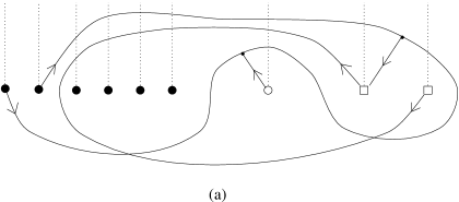
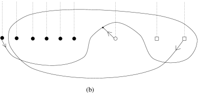
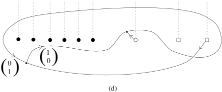
Figure 8: Multiplication of $(\mathchoice{\vbox{\vbox{\hrule height=0.6pt\hbox{\vrule width=0.6pt,height=5.0pt\kern 5.0pt\vrule width=0.6pt} \hrule height=0.6pt}}}{\vbox{\vbox{\hrule height=0.6pt\hbox{\vrule width=0.6pt,height=5.0pt\kern 5.0pt\vrule width=0.6pt} \hrule height=0.6pt}}}{\vbox{\vbox{\hrule height=0.4pt\hbox{\vrule width=0.4pt,height=2.7pt\kern 2.7pt\vrule width=0.4pt} \hrule height=0.4pt}}}{\vbox{\vbox{\hrule height=0.4pt\hbox{\vrule width=0.4pt,height=1.9pt\kern 1.9pt\vrule width=0.4pt} \hrule height=0.4pt}}}^{2}_{a},\mathchoice{\vbox{\vbox{\hrule height=0.6pt\hbox{\vrule width=0.6pt,height=5.0pt\kern 5.0pt\vrule width=0.6pt} \hrule height=0.6pt}}}{\vbox{\vbox{\hrule height=0.6pt\hbox{\vrule width=0.6pt,height=5.0pt\kern 5.0pt\vrule width=0.6pt} \hrule height=0.6pt}}}{\vbox{\vbox{\hrule height=0.4pt\hbox{\vrule width=0.4pt,height=2.7pt\kern 2.7pt\vrule width=0.4pt} \hrule height=0.4pt}}}{\vbox{\vbox{\hrule height=0.4pt\hbox{\vrule width=0.4pt,height=1.9pt\kern 1.9pt\vrule width=0.4pt} \hrule height=0.4pt}}})$ times $(\mathchoice{\vbox{\vbox{\hrule height=0.6pt\hbox{\vrule width=0.6pt,height=5.0pt\kern 5.0pt\vrule width=0.6pt} \hrule height=0.6pt}}}{\vbox{\vbox{\hrule height=0.6pt\hbox{\vrule width=0.6pt,height=5.0pt\kern 5.0pt\vrule width=0.6pt} \hrule height=0.6pt}}}{\vbox{\vbox{\hrule height=0.4pt\hbox{\vrule width=0.4pt,height=2.7pt\kern 2.7pt\vrule width=0.4pt} \hrule height=0.4pt}}}{\vbox{\vbox{\hrule height=0.4pt\hbox{\vrule width=0.4pt,height=1.9pt\kern 1.9pt\vrule width=0.4pt} \hrule height=0.4pt}}}^{4}_{a},\mathchoice{\vbox{\vbox{\hrule height=0.6pt\hbox{\vrule width=0.6pt,height=5.0pt\kern 5.0pt\vrule width=0.6pt} \hrule height=0.6pt}}}{\vbox{\vbox{\hrule height=0.6pt\hbox{\vrule width=0.6pt,height=5.0pt\kern 5.0pt\vrule width=0.6pt} \hrule height=0.6pt}}}{\vbox{\vbox{\hrule height=0.4pt\hbox{\vrule width=0.4pt,height=2.7pt\kern 2.7pt\vrule width=0.4pt} \hrule height=0.4pt}}}{\vbox{\vbox{\hrule height=0.4pt\hbox{\vrule width=0.4pt,height=1.9pt\kern 1.9pt\vrule width=0.4pt} \hrule height=0.4pt}}})$ of $su(n_{A})\times su(n_{C})$.

4.5 Construction of $E_{8}$

For the case of $E_{8}$, as we have seen in the table, there exists one representation that has no analogue for $E_{7}$, the $(7,1)_{8}$ which transforms as $(\mathchoice{\vbox{\vbox{\hrule height=0.6pt\hbox{\vrule width=0.6pt,height=5.0pt\kern 5.0pt\vrule width=0.6pt} \hrule height=0.6pt}}}{\vbox{\vbox{\hrule height=0.6pt\hbox{\vrule width=0.6pt,height=5.0pt\kern 5.0pt\vrule width=0.6pt} \hrule height=0.6pt}}}{\vbox{\vbox{\hrule height=0.4pt\hbox{\vrule width=0.4pt,height=2.7pt\kern 2.7pt\vrule width=0.4pt} \hrule height=0.4pt}}}{\vbox{\vbox{\hrule height=0.4pt\hbox{\vrule width=0.4pt,height=1.9pt\kern 1.9pt\vrule width=0.4pt} \hrule height=0.4pt}}},\cdot)$. In Fig. 9 we find an explicit open string representative for this representation by multiplying the $(\mathchoice{\vbox{\vbox{\hrule height=0.6pt\hbox{\vrule width=0.6pt,height=5.0pt\kern 5.0pt\vrule width=0.6pt} \hrule height=0.6pt}}}{\vbox{\vbox{\hrule height=0.6pt\hbox{\vrule width=0.6pt,height=5.0pt\kern 5.0pt\vrule width=0.6pt} \hrule height=0.6pt}}}{\vbox{\vbox{\hrule height=0.4pt\hbox{\vrule width=0.4pt,height=2.7pt\kern 2.7pt\vrule width=0.4pt} \hrule height=0.4pt}}}{\vbox{\vbox{\hrule height=0.4pt\hbox{\vrule width=0.4pt,height=1.9pt\kern 1.9pt\vrule width=0.4pt} \hrule height=0.4pt}}}^{2}_{a},\mathchoice{\vbox{\vbox{\hrule height=0.6pt\hbox{\vrule width=0.6pt,height=5.0pt\kern 5.0pt\vrule width=0.6pt} \hrule height=0.6pt}}}{\vbox{\vbox{\hrule height=0.6pt\hbox{\vrule width=0.6pt,height=5.0pt\kern 5.0pt\vrule width=0.6pt} \hrule height=0.6pt}}}{\vbox{\vbox{\hrule height=0.4pt\hbox{\vrule width=0.4pt,height=2.7pt\kern 2.7pt\vrule width=0.4pt} \hrule height=0.4pt}}}{\vbox{\vbox{\hrule height=0.4pt\hbox{\vrule width=0.4pt,height=1.9pt\kern 1.9pt\vrule width=0.4pt} \hrule height=0.4pt}}})$ and $(\mathchoice{\vbox{\vbox{\hrule height=0.6pt\hbox{\vrule width=0.6pt,height=5.0pt\kern 5.0pt\vrule width=0.6pt} \hrule height=0.6pt}}}{\vbox{\vbox{\hrule height=0.6pt\hbox{\vrule width=0.6pt,height=5.0pt\kern 5.0pt\vrule width=0.6pt} \hrule height=0.6pt}}}{\vbox{\vbox{\hrule height=0.4pt\hbox{\vrule width=0.4pt,height=2.7pt\kern 2.7pt\vrule width=0.4pt} \hrule height=0.4pt}}}{\vbox{\vbox{\hrule height=0.4pt\hbox{\vrule width=0.4pt,height=1.9pt\kern 1.9pt\vrule width=0.4pt} \hrule height=0.4pt}}}^{6}_{a},\mathchoice{\vbox{\vbox{\hrule height=0.6pt\hbox{\vrule width=0.6pt,height=5.0pt\kern 5.0pt\vrule width=0.6pt} \hrule height=0.6pt}}}{\vbox{\vbox{\hrule height=0.6pt\hbox{\vrule width=0.6pt,height=5.0pt\kern 5.0pt\vrule width=0.6pt} \hrule height=0.6pt}}}{\vbox{\vbox{\hrule height=0.4pt\hbox{\vrule width=0.4pt,height=2.7pt\kern 2.7pt\vrule width=0.4pt} \hrule height=0.4pt}}}{\vbox{\vbox{\hrule height=0.4pt\hbox{\vrule width=0.4pt,height=1.9pt\kern 1.9pt\vrule width=0.4pt} \hrule height=0.4pt}}})$ of $su(7)\times su(2)$. For the $(\mathchoice{\vbox{\vbox{\hrule height=0.6pt\hbox{\vrule width=0.6pt,height=5.0pt\kern 5.0pt\vrule width=0.6pt} \hrule height=0.6pt}}}{\vbox{\vbox{\hrule height=0.6pt\hbox{\vrule width=0.6pt,height=5.0pt\kern 5.0pt\vrule width=0.6pt} \hrule height=0.6pt}}}{\vbox{\vbox{\hrule height=0.4pt\hbox{\vrule width=0.4pt,height=2.7pt\kern 2.7pt\vrule width=0.4pt} \hrule height=0.4pt}}}{\vbox{\vbox{\hrule height=0.4pt\hbox{\vrule width=0.4pt,height=1.9pt\kern 1.9pt\vrule width=0.4pt} \hrule height=0.4pt}}}^{2}_{a},\mathchoice{\vbox{\vbox{\hrule height=0.6pt\hbox{\vrule width=0.6pt,height=5.0pt\kern 5.0pt\vrule width=0.6pt} \hrule height=0.6pt}}}{\vbox{\vbox{\hrule height=0.6pt\hbox{\vrule width=0.6pt,height=5.0pt\kern 5.0pt\vrule width=0.6pt} \hrule height=0.6pt}}}{\vbox{\vbox{\hrule height=0.4pt\hbox{\vrule width=0.4pt,height=2.7pt\kern 2.7pt\vrule width=0.4pt} \hrule height=0.4pt}}}{\vbox{\vbox{\hrule height=0.4pt\hbox{\vrule width=0.4pt,height=1.9pt\kern 1.9pt\vrule width=0.4pt} \hrule height=0.4pt}}})$ states we use the presentation of Fig. 3 (c), and for $(\mathchoice{\vbox{\vbox{\hrule height=0.6pt\hbox{\vrule width=0.6pt,height=5.0pt\kern 5.0pt\vrule width=0.6pt} \hrule height=0.6pt}}}{\vbox{\vbox{\hrule height=0.6pt\hbox{\vrule width=0.6pt,height=5.0pt\kern 5.0pt\vrule width=0.6pt} \hrule height=0.6pt}}}{\vbox{\vbox{\hrule height=0.4pt\hbox{\vrule width=0.4pt,height=2.7pt\kern 2.7pt\vrule width=0.4pt} \hrule height=0.4pt}}}{\vbox{\vbox{\hrule height=0.4pt\hbox{\vrule width=0.4pt,height=1.9pt\kern 1.9pt\vrule width=0.4pt} \hrule height=0.4pt}}}^{6}_{a},\mathchoice{\vbox{\vbox{\hrule height=0.6pt\hbox{\vrule width=0.6pt,height=5.0pt\kern 5.0pt\vrule width=0.6pt} \hrule height=0.6pt}}}{\vbox{\vbox{\hrule height=0.6pt\hbox{\vrule width=0.6pt,height=5.0pt\kern 5.0pt\vrule width=0.6pt} \hrule height=0.6pt}}}{\vbox{\vbox{\hrule height=0.4pt\hbox{\vrule width=0.4pt,height=2.7pt\kern 2.7pt\vrule width=0.4pt} \hrule height=0.4pt}}}{\vbox{\vbox{\hrule height=0.4pt\hbox{\vrule width=0.4pt,height=1.9pt\kern 1.9pt\vrule width=0.4pt} \hrule height=0.4pt}}})$ the presentation of Fig. 8 (e). These two representatives join suitably at one of the $C$ branes, where the string can be released. Moreover we can move the left part of the string across the leftmost $A$ brane, creating a junction and finding the representation shown in Fig. 9 (b). We can slide this junction all the way to the right, as in Fig. 9 (c), and continue to slide it until it hits the other junction, at which time we can collapse the resulting loop and obtain the presentation shown in Fig. 9 (d). Once more, we have found a one pronged object made of a closed loop and an open string, joining it to an $A$ brane. Its transformation properties under $su(n_{A})$ and $su(n_{C})$ are manifest.

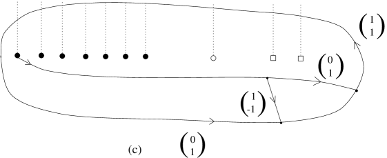
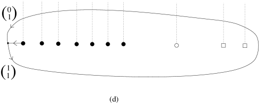
Figure 9: Multiplication of the representations $(\mathchoice{\vbox{\vbox{\hrule height=0.6pt\hbox{\vrule width=0.6pt,height=5.0pt\kern 5.0pt\vrule width=0.6pt} \hrule height=0.6pt}}}{\vbox{\vbox{\hrule height=0.6pt\hbox{\vrule width=0.6pt,height=5.0pt\kern 5.0pt\vrule width=0.6pt} \hrule height=0.6pt}}}{\vbox{\vbox{\hrule height=0.4pt\hbox{\vrule width=0.4pt,height=2.7pt\kern 2.7pt\vrule width=0.4pt} \hrule height=0.4pt}}}{\vbox{\vbox{\hrule height=0.4pt\hbox{\vrule width=0.4pt,height=1.9pt\kern 1.9pt\vrule width=0.4pt} \hrule height=0.4pt}}}^{2}_{a},\mathchoice{\vbox{\vbox{\hrule height=0.6pt\hbox{\vrule width=0.6pt,height=5.0pt\kern 5.0pt\vrule width=0.6pt} \hrule height=0.6pt}}}{\vbox{\vbox{\hrule height=0.6pt\hbox{\vrule width=0.6pt,height=5.0pt\kern 5.0pt\vrule width=0.6pt} \hrule height=0.6pt}}}{\vbox{\vbox{\hrule height=0.4pt\hbox{\vrule width=0.4pt,height=2.7pt\kern 2.7pt\vrule width=0.4pt} \hrule height=0.4pt}}}{\vbox{\vbox{\hrule height=0.4pt\hbox{\vrule width=0.4pt,height=1.9pt\kern 1.9pt\vrule width=0.4pt} \hrule height=0.4pt}}})$ and $(\mathchoice{\vbox{\vbox{\hrule height=0.6pt\hbox{\vrule width=0.6pt,height=5.0pt\kern 5.0pt\vrule width=0.6pt} \hrule height=0.6pt}}}{\vbox{\vbox{\hrule height=0.6pt\hbox{\vrule width=0.6pt,height=5.0pt\kern 5.0pt\vrule width=0.6pt} \hrule height=0.6pt}}}{\vbox{\vbox{\hrule height=0.4pt\hbox{\vrule width=0.4pt,height=2.7pt\kern 2.7pt\vrule width=0.4pt} \hrule height=0.4pt}}}{\vbox{\vbox{\hrule height=0.4pt\hbox{\vrule width=0.4pt,height=1.9pt\kern 1.9pt\vrule width=0.4pt} \hrule height=0.4pt}}}^{6}_{a},\mathchoice{\vbox{\vbox{\hrule height=0.6pt\hbox{\vrule width=0.6pt,height=5.0pt\kern 5.0pt\vrule width=0.6pt} \hrule height=0.6pt}}}{\vbox{\vbox{\hrule height=0.6pt\hbox{\vrule width=0.6pt,height=5.0pt\kern 5.0pt\vrule width=0.6pt} \hrule height=0.6pt}}}{\vbox{\vbox{\hrule height=0.4pt\hbox{\vrule width=0.4pt,height=2.7pt\kern 2.7pt\vrule width=0.4pt} \hrule height=0.4pt}}}{\vbox{\vbox{\hrule height=0.4pt\hbox{\vrule width=0.4pt,height=1.9pt\kern 1.9pt\vrule width=0.4pt} \hrule height=0.4pt}}})$ of $su(n_{A})\times su(n_{C})$. For $E_{8}$ where $su_{A}=su(7)$ the answer contains the $(\mathchoice{\vbox{\vbox{\hrule height=0.6pt\hbox{\vrule width=0.6pt,height=5.0pt\kern 5.0pt\vrule width=0.6pt} \hrule height=0.6pt}}}{\vbox{\vbox{\hrule height=0.6pt\hbox{\vrule width=0.6pt,height=5.0pt\kern 5.0pt\vrule width=0.6pt} \hrule height=0.6pt}}}{\vbox{\vbox{\hrule height=0.4pt\hbox{\vrule width=0.4pt,height=2.7pt\kern 2.7pt\vrule width=0.4pt} \hrule height=0.4pt}}}{\vbox{\vbox{\hrule height=0.4pt\hbox{\vrule width=0.4pt,height=1.9pt\kern 1.9pt\vrule width=0.4pt} \hrule height=0.4pt}}},\cdot)$.

5 Conclusions and open questions

We have shown in this paper that an open string interpretation for the gauge vectors of the exceptional Lie algebras $E_{6},E_{7}$ and $E_{8}$ can be given if multi-pronged open string are included as well as conventional open strings. The charge assignments and the transformation properties of the various states are manifest, and strings can be combined correctly by the conventional operation of joining open strings, or more precisely, open string prongs. We have also shown how some of the junction diagrams can be related to conventional open string diagrams using a modification of the Hanany-Witten effect.

We have seen that our method is powerful enough to generate very simple open string representations for the states whose conventional open string representations were not known. It is particularly striking that all states that are necessary to go beyond classical Lie algebras can be represented as closed string loops with an open string attaching it to a particular brane. $E_{6}$ requires such a loop attached to the $B$ brane, $E_{7}$ to the $B$ brane, and the $C$ branes, and $E_{8}$ to the $A$, $B$ and $C$ branes.

We have demonstrated that these configurations account for the necessary gauge vectors; however, as in previous analysis of classical groups, it is less clear under which conditions a particular open string geodesic or multi-pronged open string corresponds to a BPS state, and thus to a gauge vector.

We believe that the open string junctions are more than useful mathematical devices to account pictorially for the intricacies of the representation theory of exceptional Lie algebras. In fact, our analysis suggests that the multi-pronged open strings are the correct realization of BPS states in some regions of the moduli space of 7-brane positions. As we move in moduli space the representative of the BPS state can change, and we expect it to do so according to the crossing rules we have explained. If this physical interpretation is confirmed by further exploration, a tantalizing non-perturbative picture of open string theory including all kinds of open string junctions emerges.

References

- [1] J.E. Paton, H.M. Chan, Generalized Veneziano model with isospin, Nucl. Phys. B 10, 519 (1969); J.H. Schwarz, Gauge groups for type I superstrings, in: Proc. of the Johns Hopkins Workshop on Current Problems in Particle Theory 6, Florence, 233 (1982); N. Marcus, A. Sagnotti, Tree-level constraints on gauge groups for type I superstrings, Phys. Lett. B 119, 97 (1982).
- [2] M.R. Gaberdiel, B. Zwiebach, Tensor constructions of open string theories I: Foundations, hep-th/9705038, to appear in Nucl. Phys. B.
- [3] M. Bianchi, A. Sagnotti, On the systematics of open-string theories, Phys. Lett. B 247, 517 (1990); A. Sagnotti, Some properties of open-string theories, hep-th/9509080; E.G. Gimon, J. Polchinski, Consistency conditions for orientifolds and D manifolds, Phys. Rev. D 54, 1667 (1996), hep-th/9601038; O. Bergman, M.R. Gaberdiel, A Non-Supersymmetric Open String Theory and S-Duality, Nucl. Phys. B 499, 183 (1997), hep-th/9701137.
- [4] M.R. Gaberdiel, B. Zwiebach, Tensor constructions of open string theories II: Vector Bundles, D-branes and orientifold groups, hep-th/9707051, to appear in Phys. Lett. B.
- [5] K. Dasgupta and S. Mukhi, F-theory at constant coupling, Phys. Lett. B 385, 125 (1996), hep-th/9606044.
- [6] A. Johansen, A comment on BPS states in F-theory in 8 dimensions, Phys. Lett. B 395, 36 (1997), hep-th/9608186.
- [7] J.D. Blum, K.R. Dienes, From the type I string to M-theory: a continuous connection, hep-th/9708016.
- [8] C. Vafa, Evidence for F-theory Nucl. Phys. B 469, 403 (1996), hep-th/9602022.
- [9] A. Sen, F-theory and orientifolds, Nucl. Phys. B 475, 562 (1996), hep-th/9605150.
- [10] A. Hanany, E. Witten, Type IIB superstrings, BPS monopoles, and three-dimensional gauge dynamics, Nucl. Phys. B 492, 152 (1997), hep-th/9611230.
- [11] C. Bachas, M.R. Douglas, M.B. Green, Anomalous creation of branes, hep-th/9705074; U.H. Danielsson, G. Ferretti, I.R. Klebanov, Creation of fundamental strings by crosssing D-branes, hep-th/9705084; O. Bergman, M.R. Gaberdiel, G. Lifschytz, Branes, orientifolds and the creation of elementary strings, hep-th/9705130.
- [12] J. H. Schwarz, Lectures on Superstring and M-theory dualities, hep-th/9607201.
- [13] E. Witten, Non-commutative geometry and string field theory, Nucl. Phys. B 268, 253 (1986).
- [14] M. Saadi, B. Zwiebach, Closed string field theory from polyhedra, Ann. Phys. 192, 213 (1989); M. Kaku, Geometrical derivation of string field theory from first principles: closed strings and modular invariance, Phys. Rev. D 38, 3052 (1988); T. Kugo, H. Kunitomo, K. Suehiro, Non-polynomial closed string field theory, Phys. Lett. B 226, 48 (1989).
- [15] E. Witten , Bound states of strings and p-branes, Nucl. Phys. B 460, 335 (1996), hep-th/9510135.
- [16] M. R. Douglas, M. Li, D-brane realization of super Yang-Mills theory in four dimensions, hep-th/9604041.
- [17] O. Aharony, J. Sonnenschein, S. Yankielowicz, Interactions of strings and D-branes from M theory, Nucl. Phys. B 474, 309 (1996), hep-th/9603009.
- [18] H. Ooguri, C. Vafa, Geometry of Dualities in Four Dimensions, hep-th/9702180.
- [19] B. Greene, A. Shapere, C. Vafa, S.T. Yau, Nucl. Phys. B 337, 1 (1990).
- [20] J. H. Schwarz, An SL(2,Z) multiplet of type IIB superstrings, Phys. Lett. B 360, 13 (1995), hep-th/9508143.