BLACK HOLES IN STRING THEORY

Abstract

• Department of Physics, McGill University, Montréal, Québec
  H3A 2T8, CANADA

• Abstract. The black hole solutions to Einstein’s vacuum field equations are also solutions to the equations of motion of the low energy limit of superstring theory. At the same time, string theory boasts a much broader and richer collection of black hole solutions. Fortunately, string theories also possess a remarkable set of duality symmetries relating states within and between different string theories. These duality symmetries can be exploited to construct new black hole solutions from known solutions, giving us powerful tools with which to explore the black hole solutions of string theory. Here we introduce and demonstrate these techniques of solution generating.

• Department of Physics, McGill University, Montréal, Québec
  H3A 2T8, CANADA

• Abstract. The black hole solutions to Einstein’s vacuum field equations are also solutions to the equations of motion of the low energy limit of superstring theory. At the same time, string theory boasts a much broader and richer collection of black hole solutions. Fortunately, string theories also possess a remarkable set of duality symmetries relating states within and between different string theories. These duality symmetries can be exploited to construct new black hole solutions from known solutions, giving us powerful tools with which to explore the black hole solutions of string theory. Here we introduce and demonstrate these techniques of solution generating.

  1 INTRODUCTION

  Black holes are extremely interesting objects predicted by Einstein’s general theory of relativity as the endpoint of gravitational collapse. It has been shown that these objects possess a thermodynamic entropy [1], for which one would ideally like to have a microscopic and statistical interpretation. Classical general relativity offers no clues as to what this interpretation might be. String theory, however, is at present a strong candidate for a theory of quantum gravity. It is logical, therefore, to study black holes in the context of string theory, in the hope that some light may be shed on the physics of black holes, in particular their entropy, and in doing so validate the theory of strings as a physical theory.

  Some progress has in fact been made on this front. The dualities of strings [2] require additional objects to be added to the theory, one species of which are the $D$-branes [3]. These are objects extended in zero or more dimensions, and have been recently used to compute, for the first time, the statistical entropy of black holes. Thus it is clear that $D$-branes represent useful probes into string theory, in addition to their role in filling duality multiplets, serving as carriers of Ramond-Ramond charge [4].

  However, the $D$-brane technology is as yet applicable only to a small class of extremal, supersymmetric black holes [5, 6, 7], although the method has been applied to solutions perturbed slightly away from the extremal and supersymmetric limit [8]. One must therefore find black hole solutions for which the method applies. Here we will illustrate the methods by which black hole solutions amenable to $D$-brane analysis, and which therefore serve as a testing ground for the method, can be obtained.

  In section 2 we give a brief introduction to string theory symmetries. Section 3 then treats in detail the low energy effective actions and the duality symmetries to be used here. The procedure used to construct an example solution is then given, followed by a few remarks about the characteristics of the solution generated, a charged, rotating black hole in five spacetime dimensions.

  2 STRING THEORY SYMMETRIES

  One of the most fascinating aspects of the theory of strings is the number of symmetries [9] which can relate different regimes of a given string theory to each other, or relate one string theory to another. Recently, these have had a crucial role to play in understanding the structure of string theory. They have also led to the development of techniques which can be used to construct new solutions of the low-energy superstring equations of motion.

  

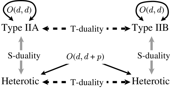
  Figure 2: An illustration of duality relations in string theory.

  Here we divide these symmetries, often known in the literature as dualities, into three main groups:

  • $O(d,d)$ symmetries are symmetries of the low-energy equations of motion which result from independence of solutions of higher compact dimensions. In a sense we can “rotate” and/or “boost” a solution in such a way that it becomes a different solution. $O(d,d)$ keeps solutions within a given string theory, rather than moving them between theories.

  • $T$-duality symmetry inverts the radius of compact dimensions, i.e., $R\to 1/R$. Because a string may wrap around a compact dimension, its spectrum of states is invariant under this change. This feature has no analog in point particle theory. $T$-duality sometimes moves a solution from one theory to another, but not always.

  • $S$-duality symmetry relates weak- and strong-coupling regimes of a string theory, or different string theories. As we will see, under $S$-dualities the string coupling constant $g=e^{\phi}$ is inverted, $g\to 1/g$, thus leading to the interchange of strong- and weak-coupling physics.

  In figure 1 we illustrate a small subset of the symmetries existing within and between string theories. For example, on the left we have an $S$-duality between the type IIA string and the heterotic string, one of a set of string/string dualities. This duality occurs in six dimensions between the heterotic string compactified from ten dimensions on the four-torus $T^{4}$, while the type IIA theory related to it is that compactified on the Calabi-Yau manifold $K3$. This duality, with $O(d,d,{\bf R})$ symmetry, will be particularly useful here.

  3 SOLUTION GENERATING

  Let us note a few salient features of low–energy actions for the heterotic and type IIA theories in six and five dimensions. We work with simplified versions of the six dimensional actions of the heterotic string compactified on $T^{4}$ and the type IIA string compactified on $K3$. All abelian gauge fields except one have been set to zero, and all scalars resulting from compactification, the moduli, are vanishing. The remaining gauge field is taken to be an internal gauge field on the heterotic side, and a Ramond–Ramond field, associated with $D$-branes, on the Type II side.

  The low energy action of the heterotic string compactified on $T^{4}$ may be written [10]:

  $$S_{h}=\int\!\!d^{6}x\sqrt{-{\cal G}_{6}}e^{-2\phi^{(h)}_{6}}\left\{R+4\big{(}\nabla\phi^{(h)}_{6}\big{)}^{2}-{{1}\over{12}}(H^{(h)}_{6})^{2}-{{1}\over{4}}{\cal F}_{6}^{2}\right\}$$ (1)

  where ${\cal G}_{6}$ is the metric, $\phi^{(h)}_{6}$ is the dilaton, $H^{(h)}_{6}$ is given by

  $$H^{(h)}_{6\,\mu\nu\lambda}=\partial_{\mu}B^{(h)}_{6\,\nu\lambda}-{{1}\over{2}}{\cal A}_{6\,\mu}{\cal F}_{6\,\nu\lambda}+({\rm cyclic})$$ (2)

  where $B^{(h)}_{6}$ is the antisymmetric tensor field and ${\cal F}_{6}=d{\cal A}_{6}$ is the field strength of the heterotic gauge field ${\cal A}_{6}$.

  For the Type IIA theory, we write the action compactified on $K3$ as

  $$S_{IIA} = \int\!\!d^{6}x\bigg{[}\sqrt{-G_{6}}\bigg{[}e^{-2\phi^{(a)}_{6}}\bigg{(}R+4\big{(}\nabla\phi^{(a)}_{6}\big{)}^{2}-{{1}\over{12}}(H^{(a)}_{6})^{2}\bigg{)}$$ (3)

  $$\qquad\quad\mbox{}-{{1}\over{4}}F_{6}^{2}\bigg{]}+{{1}\over{16}}\epsilon^{\mu\nu\lambda\rho\alpha\beta}B^{(a)}_{6\,\mu\nu}F_{6\,\lambda\rho}F_{6\,\alpha\beta}\bigg{]}$$

  where here $G_{6}$ and $\phi^{(a)}_{6}$ are the metric and dilaton, while we have

  $$H^{(a)}_{6\,\mu\nu\lambda}=\partial_{\mu}B^{(a)}_{6\,\nu\lambda}+({\rm cyclic})$$ (4)

  as the field strength of the antisymmetric tensor field $B^{(a)}_{6}$. These two actions are related by the string/string duality relation given as

  $$\phi^{(a)}_{6} = -\phi^{(h)}_{6}$$ (5)

  $$G_{6\mu\nu} = {\rm e}^{-2\phi^{(h)}_{6}}{\cal G}_{6\mu\nu}$$ (6)

  $$A_{6\mu} = {\cal A}_{6\mu}$$ (7)

  $$H^{(a)}_{6\mu\nu\rho} = {1\over 6}\epsilon_{\mu\nu\rho\sigma\kappa\delta}\,{\rm e}^{-2\phi^{(h)}_{6}}H^{(h)\,\sigma\kappa\delta}_{6},$$ (8)

  and the manifestation of strong-weak coupling exchange is then evident in (5). Since we also use the five-dimensional type IIA action compactified on $K3\otimes S^{1}$, we give here the standard Kaluza–Klein reduction on the circle $S^{1}$ with coordinate labelling $y=x^{5}$,

  $$ds_{6}^{2} = {{G}}_{\mu\nu}dx^{\mu}dx^{\nu}+e^{2\sigma}(dy+\Lambda_{G\mu}dx^{\mu})^{2}$$

  $$\phi_{6} = \phi+{{1}\over{2}}\sigma$$

  $$B_{6} = {{1}\over{2}}[B_{\mu\nu}-{{1}\over{2}}(\Lambda_{G\mu}\Lambda_{B\nu}-\Lambda_{B\mu}\Lambda_{G\nu})]dx^{\mu}\wedge dx^{\nu}+\Lambda_{B\mu}dx^{\mu}\wedge dy$$ (9)

  where $\Lambda_{G\mu}$ and $\Lambda_{B\mu}$ are the gauge fields coming from the compactification of the metric and antisymmetric tensor fields respectively. The five dimensional type IIA action (in the sector with $A_{y}=0$) is expressed in the string frame as

  $$S_{IIA} = \int\!\!d^{5}x\left[\sqrt{-G}\left[e^{-2\phi^{(a)}}\left({{R}}+4\big{(}\nabla\phi^{(a)}\big{)}^{2}-{{1}\over{12}}(H^{(a)})^{2}\right.\right.\right.$$ (10)

  $$\mbox{}\left.\left.\left.\qquad\qquad-(\partial_{\mu}\sigma)^{2}-{{1}\over{4}}e^{2\sigma}(\Xi_{G})^{2}-{{1}\over{4}}e^{-2\sigma}(\Xi_{B})^{2}\right)\right.\right.$$

  $$\mbox{}\left.\left.\qquad\qquad-{{1}\over{4}}e^{\sigma}F^{2}\right]+{{1}\over{8}}\epsilon^{\mu\nu\lambda\alpha\beta}\Lambda_{B\mu}F_{\nu\lambda}F_{\alpha\beta}\right]$$

  where $\Xi_{G}=d\Lambda_{G}$, $\Xi_{B}=d\Lambda_{B}$ and

  $$H^{(a)}_{\mu\nu\lambda}=\partial^{\vphantom{(a)}}_{\mu}B^{(a)}_{\nu\lambda}-{{1}\over{2}}\Lambda_{G\mu}\Xi_{B\nu\lambda}-{{1}\over{2}}\Lambda_{B\mu}\Xi_{G\mu\nu}+({\rm cyclic}).$$ (11)

  In five dimensions the Einstein frame metric is obtained from that appearing in (10) through the transformation $g_{\mu\nu}=e^{-4\phi/3}{G}_{\mu\nu}$.

  The solution of the five dimensional theory with which we will begin is a five dimensional black hole spinning in a single plane. It is a solution of the vacuum Einstein equations, and is found in [11]. We add a trivial flat compact dimension with coordinate $y$, and the six dimensional metric is then

  $$ds_{6}^{2} = -dt^{2}+(r^{2}+a^{2})\sin^{2}\theta d\varphi^{2}+{\beta\over{\rho^{2}}}(dt+a\sin^{2}\theta d\varphi)^{2}$$ (12)

  $$\mbox{}\qquad+{{\rho^{2}}\over{r^{2}+a^{2}-\beta}}dr^{2}+\rho^{2}d\theta^{2}+r^{2}\cos^{2}\theta d\psi^{2}+dy^{2}$$

  where $\rho^{2}=r^{2}+a^{2}\cos^{2}\theta$, and $\beta$ and $a$ are the mass and angular momentum parameters. We are using spherical polar coordinates in five dimensions, $t,r,\theta,\varphi,\psi$ with the additional coordinate $y$. This black hole is a solution of the six dimensional low energy type IIA string theory, with only the metric excited. No gauge fields, antisymmetric tensor, dilaton, or moduli fields are turned on. From it, we will obtain a charged spinning black hole solution of the type IIA theory in five dimensions, a spinning generalization of the solution in [5].

  3.1 Generating techniques

  To generate the desired black hole solution we use a series of transformations, namely $O(6,6,{\bf R})$ boosts involving the time $t$ and the circle coordinate $y$, and string/string duality. String/string duality is implemented simply by computing the mapping given in equation (8). For the $O(d,d,{\bf R})$ transformations, the procedure we have implemented is that outlined in [12]. Let us consider first the procedure for the heterotic string with one non-zero gauge field, the extension to more than one gauge field is straightforward. One first forms, from the fields of the solution with which one begins, the linear combinations

  $${K_{\pm}}_{\mu\nu}=-B^{(h)}_{\mu\nu}-{\cal G}_{\mu\nu}-{1\over 4}{\cal A}_{\mu}{\cal A}_{\nu}\pm\eta_{\mu\nu}$$ (13)

  from which the following matrix is constructed

  $${\cal M}=\left(\begin{array}[]{ccc}K_{-}^{t}{\cal G}^{-1}K_{-}&K_{-}^{t}{\cal G}^{-1}K_{+}&-K_{-}^{t}{\cal G}^{-1}{\cal A}\\ K_{+}^{t}{\cal G}^{-1}K_{-}&K_{+}^{t}{\cal G}^{-1}K_{+}&-K_{+}^{t}{\cal G}^{-1}{\cal A}\\ -{\cal A}^{t}{\cal G}^{-1}K_{-}&-{\cal A}^{t}{\cal G}^{-1}K_{+}&{\cal A}^{t}{\cal G}^{-1}{\cal A}\end{array}\right)$$ (17)

  where the superscript ^t indicates the transpose. At this point the effect of an $O(d,d,{\bf R})$ transformation on the solution in question is contained in the relation

  $${\cal M}\rightarrow\tilde{\cal M}=\Omega_{d}{\cal M}\Omega_{d}^{t}$$ (18)

  where the transformation matrix $\Omega_{d}\in O(d,d,{\bf R})$.

  After equation (16) has been computed, there remains the question of extracting the new metric and other fields from the new matrix ${\tilde{\cal M}}$. The way to do this is also found in [12] and consists of forming the matrix

  $$V=\left(\begin{array}[]{ccc}\eta/2&-\eta/2&0\\ 1/2&1/2&0\\ 0&0&1/\sqrt{2}\end{array}\right)$$ (19)

  which leaves $\tilde{\cal M}$ in a state looking like

  $${\tilde{\cal M}}^{\prime}=V\tilde{\cal M}V^{t}=\left(\begin{array}[]{ccc}{{\cal G}^{\prime}}^{-1}&-{{\cal G}^{\prime}}^{-1}K^{\prime}&{{\cal G}^{\prime}}^{-1}{{\cal A}}^{\prime}/\sqrt{2}\\ -{K^{\prime}}^{t}{{\cal G}^{\prime}}^{-1}&{K^{\prime}}^{t}{{\cal G}^{\prime}}^{-1}K^{\prime}&-{K^{\prime}}^{t}{{\cal G}^{\prime}}^{-1}{{\cal A}}^{\prime}/\sqrt{2}\\ {{{\cal A}}^{\prime}}^{t}{{\cal G}^{\prime}}^{-1}/\sqrt{2}&-{{{\cal A}}^{\prime}}^{t}{{\cal G}^{\prime}}^{-1}K^{\prime}/\sqrt{2}&{{{\cal A}}^{\prime}}^{t}{{\cal G}^{\prime}}^{-1}{\cal A}/2\\ \end{array}\right)$$ (20)

  where $K^{\prime}=({K^{\prime}}_{\pm}\mp\eta)$ and therefore the new metric, new $K^{\prime}$, and gauge field $A$ can be extracted from the upper left, upper center, and upper right parts respectively of $\tilde{\cal M}^{\prime}$. Then the antisymmetric tensor field and dilaton are

  $${B^{(h)}}^{\prime}=\,-{1\over 2}(K^{\prime}-{K^{\prime}}^{t}),\qquad\qquad{\rm e}^{2{\phi^{(h)}}^{\prime}}=\,{\det{\cal G}^{\prime}\over\det{\cal G}}{\rm e}^{2{\phi^{(h)}}}.$$ (21)

  For the heterotic string the group under which the equations of motion of the low energy effective action are invariant is $O(d,d+p,{\bf R})$ where $d$ is the number of coordinates in the full ten dimensional theory with respect to which the solution is independent, and $p$ can be thought of as the number of gauge fields in the solution. In the present case, therefore, on the heterotic side the group in question is $O(6,7,{\bf R})$.

  What of the type IIA side of the story? $T$-duality, when applied to a type II solution changes its chirality, altering its Ramond-Ramond field content. Since $T$-duality is in the $O(d,d,{\bf Z})$ subgroup of $O(d,d,{\bf R})$, it is not possible to carry out the more general $O(d,d,{\bf R})$ transformations on the RR sector. Therefore, one can apply this technique to the type II theories only when the Ramond-Ramond fields all vanish. In this case the formulae (13) through (19) apply when all ${\cal A}^{(1)\,\alpha}=0$, giving $O(6,6,{\bf R})$ symmetry.

  Let us now outline the series of steps that will produce our new solution. We begin with the metric (12) as a string-frame type IIA solution in six dimensions. We apply an $O(6,6)$ boost mixing the $(t,y)$ directions, following the five dimensional black hole construction of [13]. This causes the resulting six–dimensional solution to have no $G_{6\,y\mu}$ for $\mu<5$, but induces a $B^{(a)}_{6yt}$ and a $\phi^{(a)}_{6}$.

  The next step is to apply string/string duality to create a heterotic solution from the type IIA solution. This is done by applying the mapping (8), after which the new $B^{(h)}$ is computed up to gauge transformations by integrating the field strength $H^{(h)}$. Using now the $O(6,7)$ symmetry we apply a second boost, mixing the time $t$ and the internal direction involving ${\cal A}_{6}$, with parameter $z$. String/string duality is then applied a second time to convert the heterotic solution back to a Type IIA solution, followed by the standard Kaluza–Klein reduction to five dimensions as given in (9), which in turn is followed by transformation to the Einstein frame.

  The above boost parameters $x$ and $z$ are carefully chosen to satisfy $z=2x^{2}-1$ which reduces the five dimensional dilaton to a constant. The resulting configuration is a charged spinning five dimensional black hole with constant dilaton. This solution is quite complicated and will not be written here, but it simplifies substantially in the extremal limit.

  3.2 The extremal black hole

  The extremal limit of the black hole is computed by taking the boost parameter $x$ off to infinity, and simultaneously the mass parameter $\beta$ and the angular momentum parameter $a$ to zero such that the quantities

  $$\lim_{\stackrel{{\scriptstyle\scriptstyle x\to\infty}}{{\beta\to 0}}}\beta\,x^{2}\equiv\,\mu,\qquad\qquad\lim_{\stackrel{{\scriptstyle\scriptstyle x\to\infty}}{{a\to 0}}}a\,x\equiv\,\omega,$$ (22)

  remain finite, where $\beta,a$ are the quantities appearing in the metric (12). After doing a coordinate transformation to match with [5], $r^{2}\to r^{2}+\mu$, we obtain for the extremal metric and gauge fields

  $$ds_{5}^{2} = -{\left(1-{\mu\over{r^{2}}}\right)^{2}}\left[dt-{{\mu\omega\sin^{2}\theta}\over{(r^{2}-\mu)}}d\varphi+{{\mu\omega\cos^{2}\theta}\over{(r^{2}-\mu)}}d\psi\right]^{2}$$ (23)

  $$\mbox{}+\left(1-{\mu\over{r^{2}}}\right)^{-2}\!dr^{2}\!+\!r^{2}(d\theta^{2}+\sin^{2}\theta d\varphi^{2}+\cos^{2}\theta d\psi^{2})$$

  $${A} = {\sqrt{2}\over\lambda}{{\mu}\over{r^{2}}}\bigg{(}dt+\omega\sin^{2}\theta d\varphi-\omega\cos^{2}\theta d\psi\bigg{)}$$ (24)

  $${\Lambda_{B}} = {{\lambda^{3}}\over{\sqrt{2}}}{A}$$ (25)

  $$e^{\sigma+2\phi^{(a)}/3} = \lambda^{2}.$$ (26)

  While the result of our solution generating procedure yields zero dilaton and modulus, $\phi^{(a)}=0=\sigma$, we have shifted these scalars by a constant to those of (24), which introduces the scaling of the gauge fields by $\lambda$ given above [5]. The above fields are the only ones excited in this black hole background. Notice that when we take $\omega\to 0$, we recover the solution of [5].

  3.3 Properties of the solution

  The angular momenta in the independent planes defined by $\varphi,\psi$ are

  $$J_{1}\equiv J_{\varphi}=+{\pi\over{4}}\mu\omega,\qquad\qquad J_{2}\equiv J_{\psi}=-{\pi\over{4}}\mu\omega$$ (27)

  and for the ADM mass we find

  $$M_{ADM}={{3\pi\mu}\over{4}},$$ (28)

  while the charges under the form fields $\Xi$ and $F$ are

  $$q_{\Xi} \equiv {{1}\over{4\pi^{2}}}\int_{S^{3}}{}^{\star}(e^{-2\sigma-4\phi^{(a)}/3}\,\Xi_{B})=\mu/\lambda^{2},$$

  $$q_{F} \equiv {{1}\over{16\pi}}\int_{S^{3}}{}^{\star}(e^{\sigma+2\phi^{(a)}/3}F)=-{{\pi}\over{2\sqrt{2}}}\mu\,\lambda.$$ (29)

  Note that this black hole, although a solution of the low–energy string theory equations, is not a solution of the Einstein–Maxwell equations in five dimensions. In the spinning configuration, the magnetic dipole field combines with the electric monopole field so that the Chern–Simons contributions to the equations of motion are nontrivial.

  Let us now obtain the classical entropy of this extremal spinning black hole. In the above coordinates, the horizon is at $r=r_{0}=\sqrt{\mu}$, and its entropy is found to be ($|J_{1}|=|J_{2}|\equiv J$)

  $${\cal S}={{1}\over{2}}\pi^{2}\mu\sqrt{\mu-\omega^{2}}=2\pi\sqrt{{{q_{\Xi}\,q_{F}^{2}}\over{2}}-J^{2}}$$ (30)

  where in the second line we have written the entropy in terms of the physical charges and angular momenta. Note that both of these expressions are independent of $\lambda$. Counting of the entropy from a microscopic standpoint using $D$-brane methods reproduces exactly this result [7].

  This extremal rotating charged black hole has a horizon with finite area, a feature not easy to find. Ordinarily the addition of rotation (without energy) to an extremal Reissner-Nordstrom black hole destabilizes the horizon and yields a naked singularity. However string theory stabilizes the horizon with the help of a Chern-Simons coupling in the low-energy field theory.

  4 CONCLUSIONS

  We have demonstrated here the utility of the symmetries of low energy effective string theory in the construction of novel black hole solutions. Thus these symmetries have a very practical application, allowing us in effect to solve the equations of motion of string theory using purely algebraic methods. A demonstration of the power of these symmetry methods was made by constructing a new class of five-dimensional supersymmetric rotating black hole solutions.

  One might say that the symmetries of string theory do triple duty. First, they require the inclusion in string theory of additional states beyond fundamental strings called $D$-branes, which carry Ramond-Ramond charge. These $D$-branes allow us to compute from a microscopic, statistical standpoint the entropy of at least particular classes of black holes. Second, the symmetries give rise to methods of solution generating by which new black hole solutions may be constructed. It is then possible to construct new black hole solutions which fall into those classes to which the $D$-brane methods apply, namely (near) supersymmetric black holes, allowing the methods to be thoroughly tested. Third, these benefits of a more immediate and practical nature come in addition to the role these symmetries play in our further discovery of the structure of the theory of strings.

  ACKNOWLEDGEMENTS

  The author would like to thank R.C. Myers, R.R. Khuri and N. Kaloper for helpful discussions and constructive criticism. The financial support of NSERC of Canada and le Fonds FCAR du Québec is also appreciated.

References

-
[1]
Bekenstein, J.D., 1973,
Phys. Rev. D7, 2333;
Hawking, S.W., 1975 Commmun. Math. Phys. 43, 199. -
[2]
Duff, M.J., 1996,
Int. J. Mod. Phys. A11, 5623;
Schwarz, J.H., 1997, Nucl. Phys. Proc. Suppl. 55B 1. -
[3]
Johnson, C.V., 1997,
Nucl. Phys. Proc. Suppl. 52A, 326;
Polchinski, J., 1996, TASI Lectures on -branes, lectures at TASI-96, Boulder, Colorado, e-print hep-th/9611050. - [4] Polchinski, J., 1995, Phys. Rev. Lett. 75, 4724
- [5] Strominger, A. and Vafa, C., 1996, Phys. Lett. B379, 99.
- [6] Horowitz, G.T. and Strominger, A., 1996, Phys. Rev. Lett. 77, 2368.
- [7] Breckenridge, J.C., Myers, R.C., Peet, A.W. and Vafa, C., 1997, Phys. Lett. B391, 93.
-
[8]
Horowitz, G.T., Maldacena, J.M. and Strominger, A., 1996,
Phys. Lett. B383, 151;
Breckenridge, J.C., Lowe, D.A., Myers, R.C., Peet, A.W., Strominger, A. and Vafa, C., 1996, Phys. Lett. B381, 423. - [9] Giveon, A., Porrati, M. and Rabinovici, E., 1994, Phys. Rep. 244, 77.
- [10] Sen, A., 1994, Int. J. Mod. Phys. A9, 3707.
- [11] Myers, R.C. and Perry, M.J., 1986, Ann. Phys. 12, 304.
- [12] Hassan, S.F. and Sen, A., 1992, Nucl. Phys. B375, 103.
- [13] Horowitz, G.T. and Sen, A., 1996, Phys. Rev. D53, 808.
-