CERN-TH/97-217

hep-th/9708130

INTRODUCTION TO NON-PERTURBATIVE STRING THEORY

Elias Kiritsis Theory Division, CERN, CH-1211
Geneva 23, SWITZERLAND

A brief introduction to the non-perturbative structure of string theory is presented. Various non-perturbative dualities in ten and six dimensions as well as D-branes are discussed.

Lectures presented at the CERN-La Plata-Santiago de Compostella School of Physics, La Plata, May 1997.

CERN-TH/97-217

May 1997

1 Non-perturbative string dualities: a foreword

In these lectures I will give a brief guide to some recent developments towards understanding the non-perturbative aspects of string theories. There was a parallel developement in the context of supersymmetric field theories, [1, 2]. We will not discuss here the field theory case. The interested reader may consult several comprehensive review articles [3, 4]. We would point out however that the field theory non-perturbative dynamics is naturally understood in the context of string theory and there was important cross-fertilization between the two disciplines.

In ten dimensions there are five distinct consistent supersymmetric string theories, type-IIA,B, heterotic (O(32),E${}_{8}\times$E₈) and the unoriented O(32) type I theory that contains also open strings. The two type-II theories have N=2 supersymmetry while the others only N=1. An important question we would like to address is: Are these strings theories different or just different aspects of the same theory?

In fact, by compactifying one dimension on a circle we can show that we can connect the two heterotic theories as well as the two type-II theories. This is schematically represented with the broken arrows in Fig. 1.

We will first show how the heterotic O(32) and E${}_{8}\times$E₈ theories are connected in $D=9$. Upon compactification on a circle of radius $R$ we can also turn on 16 Wilson lines. The partition function of the O(32) heterotic theory then can be written as

$$Z^{\rm O(32)}_{D=9}={1\over(\sqrt{\tau_{2}}\eta\bar{\eta})^{7}}{\Gamma_{1,17}(R,Y^{I})\over\eta\bar{\eta}^{17}}~{}{1\over 2}\sum_{a,b=0}^{1}~{}(-1)^{a+b+ab}~{}{\vartheta^{4}[^{a}_{b}]\over\eta^{4}}\,,$$ (1.1)

where the lattice sum $\Gamma_{p,p+16}$ is

$$Z_{p,p+16}(G,B,Y)={\sqrt{{\rm det~{}G}}\over\tau_{2}^{p/2}\eta^{p}\bar{\eta}^{p+16}}\sum_{m^{\alpha},n^{\alpha}\in Z}\exp\left[-{\pi\over\tau_{2}}(G+B)_{\alpha\beta}(m^{\alpha}+\tau n^{\alpha})(m^{\beta}+\bar{\tau}n^{\beta})\right]\times$$ (1.2)

$$\times{1\over 2}\sum_{a,b=0}^{1}~{}\prod_{I=1}^{16}~{}e^{i\pi(m^{\alpha}Y^{I}_{\alpha}Y^{I}_{\beta}n^{\beta}-b~{}n^{\alpha}Y^{I}_{\alpha})}~{}\bar{\vartheta}\left[{}^{a-2n^{\alpha}Y^{I}_{\alpha}}_{b-2m^{\beta}Y^{I}_{\beta}}\right]$$

We will focus on some special values for the Wilson lines $Y^{I}$, namely we will take eight among them to be zero and the other eight to be 1/2. Then, the lattice sum (in Lagrangian representation) can be rewritten as

$$\Gamma_{1,17}(R)=R\sum_{m,n\in Z}\exp\left[-{\pi R^{2}\over\tau_{2}}|m+\tau n|^{2}\right]{1\over 2}\sum_{a,b}~{}\bar{\vartheta}^{8}[^{a}_{b}]~{}\bar{\vartheta}^{8}[^{a+n}_{b+m}]$$

$$={1\over 2}\sum_{h,g=0}^{1}\Gamma_{1,1}(2R)[^{h}_{g}]~{}{1\over 2}\sum_{a,b}~{}\bar{\vartheta}^{8}[^{a}_{b}]~{}\bar{\vartheta}^{8}[^{a+h}_{b+g}]\,,$$ (1.3)

where $\Gamma_{1,1}[^{h}_{g}]$ are the $Z_{2}$ translation blocks of the circle partition function

$$\Gamma_{1,1}(R)[^{h}_{g}]=R\sum_{m,n\in Z}\exp\left[-{\pi R^{2}\over\tau_{2}}\left|\left(m+{g\over 2}\right)+\tau\left(n+{h\over 2}\right)\right|^{2}\right]$$ (1.4)

$$={1\over R}\sum_{m,n\in Z}~{}(-1)^{mh+ng}~{}\exp\left[-{\pi\over\tau_{2}R^{2}}|m+\tau n|^{2}\right]\,.$$ (1.5)

In the $R\to\infty$ limit (1.4) implies that only $(h,g)=(0,0)$ contributes in the sum in (1.3) and we end up with the O(32) heterotic string in ten dimensions. In the $R\to 0$ limit the theory decompactifies again, but from (1.5) we deduce that all $(h,g)$ sectors contribute equally in the limit. The sum on $(a,b)$ and $(h,g)$ factorizes and we end up with the E${}_{8}\times$ E₈ theory in ten dimensions. Both theories are different limiting points (boundaries) in the moduli space of toroidally compactified heterotic strings.

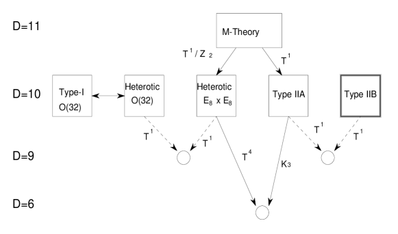
Figure 1: The Web of duality symmetries between string theories. Broken lines correspond to perturbative duality connections. Type-IIB in ten dimensions is supposed to be self-dual under SL(2,ℤ).

In the type-II case the situation is similar. We compactify on a circle. Under an $R\to 1/R$ duality

$$\partial X^{9}\to\partial X^{9}\;\;\;,\;\;\;\psi^{9}\to\psi^{9}\;\;\;,\;\;\;\bar{\partial}X^{9}\to-\bar{\partial}X^{9}\;\;\;,\;\;\;\bar{\psi}^{9}\to-\bar{\psi}^{9}\,.$$ (1.6)

Due to the change of sign of $\bar{\psi}^{9}$ the projection in the $\bar{R}$ sector is reversed. Consequently the duality maps type-IIA to type-IIB and vice versa. We can also phrase this in the following manner: The $R\to\infty$ limit of the toroidally compactified type-IIA string gives the type-IIA theory in ten dimensions. The $R\to 0$ limit gives the type-IIB theory in ten dimensions.

Apart from these perturbative connections, today we have evidence that all supersymmetric string theories are connected. Since they look very different in perturbation theory, the connections must necessarily involve strong coupling.

First, there is evidence that the type-IIB theory has an SL(2,ℤ) symmetry which, among other things, inverts the coupling constant [5, 6]. Consequently, the strong coupling limit of type-IIB is given also by the weakly-coupled type-IIB theory. Upon compactification, this symmetry combines with the perturbative $T$-duality symmetries to produce a large discrete duality group known as the $U$-duality group, which is the discretization of the non-compact continuous symmetries of the maximal effective supergravity theory. In table 3 below, the $U$-duality groups are given for various dimensions. They were conjecture to be exact symmetries in [6]. A similar remark applies to non-trivial compactifications.

Dimension SUGRA symmetry T-duality U-duality 10A SO(1,1,ℝ)/Z₂ 1 1 10B SL(2,ℝ) 1 SL(2,ℤ) 9 SL(2,ℝ)$\times$O(1,1,ℝ) Z₂ SL(2,ℤ)$\times$Z₂ 8 SL(3,ℝ)$\times$SL(2,ℝ) O(2,2,ℤ) SL(3,ℤ)$\times$SL(2,ℤ) 7 SL(5,ℝ) O(3,3,ℤ) SL(5,ℤ) 6 O(5,5,ℝ) O(4,4,ℤ) O(5,5,ℤ) 5 E₆₍₆₎ O(5,5,ℤ) E₆₍₆₎(ℤ) 4 E₇₍₇₎ O(6,6,ℤ) E₇₍₇₎(ℤ) 3 E₈₍₈₎ O(7,7,ℤ) E₈₍₈₎(ℤ)

Table 3: Duality symmetries for the compactified type-II string.

Also, it can be argued that the strong coupling limit of type-IIA theory is described by an eleven-dimensional theory named “M-theory” [7]. Its low-energy limit is eleven-dimensional supergravity. Compactification of M-theory on circle with very small radius gives the perturbative type-IIA theory.

If instead we compactify M-theory on the $Z_{2}$ orbifold of the circle $T^{1}/Z_{2}$ then we obtain the heterotic E${}_{8}\times$E₈ theory, [8]. When the circle is large the heterotic theory is strongly coupled while for small radius it is weakly coupled.

Finally, the strong coupling limit of the O(32) heterotic string theory is the type I O(32) theory and vice versa, [9].

There is another non-trivial non-perturbative connection in six dimensions: The strong coupling limit of the six-dimensional toroidally compactified heterotic string is given by the type-IIA theory compactified on K3 and vice versa [6].

Thus, we are led to suspect that there is an underlying “universal” theory whose various limits in its “moduli” space produce the weakly coupled ten-dimensional supersymmetric string theories as depicted in Fig. 2 (borrowed from [10]). The correct description of this theory is unknown although there is a proposal that it might have a matrix description [11], inspired from D-branes [12], which reproduces the perturbative IIA string in ten dimensions [13].

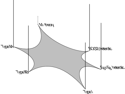
Figure 2: A unique theory and its various limits.

We will provide with a few more explanations and arguments supporting the non-perturbative connections mentioned above. But before we get there, we will need some “non-perturbative tools”, namely the notion of BPS states and p-branes, which I will briefly describe.

2 Antisymmetric tensors and p-branes .

The various string theories have massless antisymmetric tensors in their spectrum. We will use the language of forms and we will represent a rank-$p$ antisymmetric tensor $A_{\mu_{1}\mu_{2}\ldots\mu_{p}}$ by the associated $p$-form

$$A_{p}\equiv A_{\mu_{1}\mu_{2}\ldots\mu_{p}}dx^{\mu_{1}}\wedge\ldots\wedge dx^{\mu_{p}}\,.$$ (2.1)

Such $p$-forms transform under generalized gauge transformations:

$$A_{p}\to A_{p}+d~{}\Lambda_{p-1},\,,$$ (2.2)

where $d$ is the exterior derivative ($d^{2}=0$) and $\Lambda_{p-1}$ is a $(p-1)$-form which serves as the parameter of gauge transformations. The familiar case of (abelian) gauge fields corresponds to $p=1$. The gauge invariant field strength is

$$F_{p+1}=d~{}A_{p}\,.$$ (2.3)

satisfying the free Maxwell equations

$$d^{*}F_{p+1}=0$$ (2.4)

The natural objects, charged under a $(p+1)$-form $A_{p+1}$ are $p$-branes. A $p$-brane is an extended object with $p$ spatial dimensions. Point particles correspond to $p=0$, strings to $p=1$. The natural coupling of $A_{p+1}$ and a $p$-brane is given by

$$\exp\left[iQ_{p}\int_{\rm world-volume}A_{p+1}\right]=\exp\left[iQ_{p}\int A_{\mu_{0}\ldots\mu_{p}}dx^{\mu_{0}}\wedge\ldots\wedge dx^{\mu_{p}}\right]\,,$$ (2.5)

which generalizes the Wilson line coupling in the case of electromagnetism. The world-volume of $p$-brane is $p+1$-dimensional. Note also that this is precisely the $\sigma$-model coupling of the usual string to the NS antisymmetric tensor. The charge $Q_{p}$ is the usual electric charge for $p=0$ and the string tension for $p=1$. For the $p$-branes we will be considering, the (electric) charges will be related to their tensions (mass per unit volume).

In analogy with electromagnetism, we can also introduce magnetic charges. First, we must define the analog of the magnetic field: the magnetic (dual) form. This is done by first dualizing the field strength and then rewriting it as the exterior derivative of another form :

$$d\tilde{A}_{D-p-3}=\tilde{F}_{D-p-2}=^{*}F_{p+2}=^{*}dA_{p+1}\,,$$ (2.6)

where $D$ is the the dimension of spacetime. Thus, the dual (magnetic) form couples to $(D-p-4)$-branes that play the role of magnetic monopoles with “magnetic charges” $\tilde{Q}_{D-p-4}$.

There is a generalization of the Dirac quantization condition to general p-form charges discovered by Nepomechie and Teitelboim, [14]. The argument parallels that of Dirac. Consider an electric p-brane with charge $Q_{p}$ and a magnetic $(D-p-4)$-brane with charge $\tilde{Q}_{D-p-4}$. Normalize the forms so that the kinetic term is ${1\over 2}\int^{*}F_{p+2}F_{p+2}$. Integrating the field strength $F_{p+2}$ on a $(D-p-2)$-sphere surrounding the $p$-brane we obtain the total flux $\Phi=Q_{p}$. We can also write

$$\Phi=\int_{S^{D-p-2}}~{}^{*}F_{p+2}=\int_{S^{D-p-3}}~{}\tilde{A}_{D-p-3}\,,$$ (2.7)

where we have used (2.6) and we have integrated around the “Dirac string”. When the magnetic brane circles the Dirac string it picks up a phase $e^{i\Phi\tilde{Q}_{D-p-4}}$ as can be seen from (2.5). Unobservability of the string implies the Dirac-Nepomechie-Teitelboim quantization condition

$$\Phi\tilde{Q}_{D-p-4}=Q_{p}\tilde{Q}_{D-p-4}=2\pi N\;\;\;,\;\;\;n\in Z\,.$$ (2.8)

3 BPS states and bounds

The notion of BPS states is of capital importance in discussions of non-perturbative duality symmetries. Massive BPS states appear in theories with extended supersymmetry. It just happens that sometimes supersymmetry representations are shorter than usual. This is due to some of the supersymmetry operators being “null” so that they cannot create new states. The vanishing of some supercharges depends on the relation between the mass of a multiplet and some central charges appearing in the supersymmetry algebra. These central charges depend on electric and magnetic charges of the theory as well as expectation values of scalars (moduli). In a sector with given charges, the BPS states are the lowest lying states and they saturate the so-called BPS bound which for point-like states is of the form

$$M\geq~{}{\rm maximal~{}~{}eigenvalue~{}~{}of}\;\;Z\,,$$ (3.1)

where $Z$ is the central charge matrix. This is shown in appendix B where we discuss in detail the representations of extended supersymmetry in four dimensions.

BPS states behave in very special way.

$\bullet$ At generic points in moduli space they are absolutely stable. The reason is the dependence of their mass on conserved charges. Charge and energy conservation prohibits their decay. Consider as an example, the BPS mass formula

$$M^{2}_{m,n}={|m+n\tau|^{2}\over\tau_{2}}\;\;,$$ (3.2)

where $m,n$ are integer valued conserved charges, and $\tau$ is a complex modulus. This BPS formula is relevant for N=4, SU(2) gauge theory, in a subspace of its moduli space. Consider a BPS state with charges $(m_{0},n_{0})$, at rest, decaying into N states with charges $(m_{i},n_{i})$ and masses $M_{i}$, $i=1,2,\cdots,N$. Charge conservation implies, that $m_{0}=\sum_{i=1}^{N}m_{i}$, $n_{0}=\sum_{i=1}^{N}n_{i}$. The four-momenta of the particles produced are $(\sqrt{M_{i}^{2}+\vec{p}_{i}^{2}},\vec{p}_{i})$ with $\sum_{i=1}^{N}\vec{p}_{i}=\vec{0}$. Conservation of energy implies

$$M_{m_{0},n_{0}}=\sum_{i=1}^{N}\sqrt{M_{i}^{2}+\vec{p}^{2}_{i}}\geq\sum_{i=1}^{N}M_{i}\;\;.$$ (3.3)

Also in a given charge sector (m,n) the BPS bound implies that any mass $M\geq M_{m,n}$ with $M_{m,n}$ given in (3.2). Thus, from (3.3) we obtain

$$M_{m_{0},n_{0}}\geq\sum_{i=1}^{N}M_{m_{i},n_{i}}\;\;,$$ (3.4)

and the equality will hold if all particles are BPS and are produced at rest ($\vec{p}_{i}=\vec{0}$). Consider now the two-dimensional vectors $v_{i}=m_{i}+\tau n_{i}$ on the complex $\tau$-plane, with length $||v_{i}||^{2}=|m_{i}+n_{i}\tau|^{2}$. They satisfy, $v_{0}=\sum_{i=1}^{N}v_{i}$. Repeated application of the triangle inequality implies

$$||v_{0}||\leq\sum_{i=1}^{N}||v_{i}||\;\;.$$ (3.5)

This is incompatible with energy conservation (3.4) unless all vectors $v_{i}$ are parallel. This will happen only if $\tau$ is real. For energy conservation it should also be a rational number. On the other hand, due to the SL(2,ℤ) invariance of (3.2), the inequivalent choices for $\tau$ are in the SL(2,$\hbox{\mybb Z})$ fundamental domain and $\tau$ is never real there. In fact, real rational values of $\tau$ are mapped by SL(2,$\hbox{\mybb Z})$ to $\tau_{2}=\infty$, and since $\tau_{2}$ is the inverse of the coupling constant, this corresponds to the degenerate case of zero coupling. Consequently, for $\tau_{2}$ finite, in the fundamental domain, the BPS states of this theory are absolutely stable. This is always true in theories with more than 8 conserved supercharges (corresponding to N$>2$ supersymmetry in four dimensions). In cases, corresponding to theories with 8 supercharges, there are regions in the moduli space, where BPS states, stable at weak coupling, can decay at strong coupling. However, there is always a large region around weak coupling, where they are stable.

$\bullet$ The mass-formula of BPS states is supposed to be exact if one uses renormalized values for the charges and moduli. The argument is that quantum corrections would spoil the relation of mass and charges and if we assume unbroken SUSY at the quantum level that would give incompatibilities with the dimension of their representations. Of course this argument seems to have a loophole: a specific set of BPS multiplets can combine into a long one. In that case, the argument above does not prohibit corrections. Thus, we have to count BPS states modulo long supermultiplets. This is precisely what helicity supertrace formulae do for us. They are reviewed in detail in appendix B. Even in the case of N=1 supersymmetry there is an analog of BPS states, namely the massless states.

There are several amplitudes that in perturbation theory obtain contributions from BPS states only. In the case of 8 conserved supercharges (N=2 supersymmetry in four dimensions), all two-derivative terms as well as $R^{2}$ terms are of that kind. In the the case of 16 conserved supercharges (N=4 supersymmetry in four dimensions) except the terms above, also the four derivative terms as well as $R^{4}$, $R^{2}F^{2}$ terms are of a similar kind. The normalization argument of the BPS mass formula makes another important assumption: That as the coupling grows, there is no phase transition during which supersymmetry is (partially) broken.

The BPS states described above can be realized as point-like soliton solutions of the relevant effective supergravity theory. The BPS condition is the statement that the soliton solution leaves part of the supersymmetry unbroken. The unbroken generators do not change the solution, while the broken ones generate the supermultiplet of the soliton which is thus shorter than the generic supermultiplet.

So far we discussed point-like BPS states. There are however BPS versions for extended objects (BPS p-branes). In the presence of extended objects the supersymmetry algebra can acquire central charges that are not Lorentz scalars (as we assumed in Appendix B). Their general form can be obtained from group theory in which case we deduce that they must be antisymmetric tensors, $Z_{\mu_{1}\ldots\mu_{p}}$. Such central charges have values proportional to the charges $Q_{p}$ of p-branes. Then, the BPS condition would relate these charges with the energy densities (p-brane tensions) $\mu_{p}$ of the relevant p-branes. Such p-branes can be viewed as extended soliton solutions of the effective theory. The BPS condition is the statement that the soliton solution leaves some of the supersymmetries unbroken.

4 Massless RR states

We will now consider in more detail the massless R-R states of type-IIA,B string theory, since they have unusual properties and play a central role in non-perturbative duality symmetries. The reader is referred to [15] for further reading.

I will first start by describing in detail the $\Gamma$-matrix conventions in flat ten-dimensional Minkowski space [16].

The $32\times 32$-dimensional $\Gamma$-matrices satisfy

$$\{\Gamma^{\mu},\Gamma^{\nu}\}=-2\eta^{\mu\nu}\;\;\;,\;\;\;\eta^{\mu\nu}=(-++\ldots+)\,.$$ (4.1)

The $\Gamma$-matrix indices are raised and lowered with the flat Minkowski metric $\eta^{\mu\nu}$.

$$\Gamma_{\mu}=\eta_{\mu\nu}\Gamma^{\nu}\;\;\;\,\;\;\;\Gamma^{\mu}=\eta^{\mu\nu}\Gamma_{\nu}\;.$$ (4.2)

We will be in the Majorana representation where the $\Gamma$-matrices are pure imaginary, $\Gamma^{0}$ is antisymmetric, the rest symmetric. Also

$$\Gamma^{0}\Gamma_{\mu}^{\dagger}\Gamma^{0}=\Gamma_{\mu}\;\;\;,\;\;\;\Gamma^{0}\Gamma_{\mu}\Gamma^{0}=-\Gamma_{\mu}^{T}\,.$$ (4.3)

Majorana spinors $S_{\alpha}$ are real: $S^{*}_{\alpha}=S_{\alpha}$.

$$\Gamma_{11}=\Gamma_{0}\ldots\Gamma_{9}\;\;\;,\;\;\;(\Gamma_{11})^{2}=1\;\;\;,\;\;\;\{\Gamma_{11},\Gamma^{\mu}\}=0\,.$$ (4.4)

$\Gamma_{11}$ is symmetric and real. This is the reason that in ten dimensions the Weyl condition $\Gamma_{11}S=\pm S$ is compatible with the Majorana condition. We use the convention that for the Levi-Civita tensor, $\epsilon^{01\ldots 9}=1$. We will define the antisymmetrized products of $\Gamma$-matrices

$$\Gamma^{\mu_{1}\ldots\mu_{k}}={1\over k!}\Gamma^{[\mu_{1}}\ldots\Gamma^{\mu_{k}]}={1\over k!}\left(\Gamma^{\mu_{1}}\ldots\Gamma^{\mu_{k}}\pm{\rm permutations}\right)\,.$$ (4.5)

We can derive by straightforward computation the following identities among $\Gamma$-matrices:

$$\Gamma_{11}\Gamma^{\mu_{1}...\mu_{k}} = {(-1)^{[{k\over 2}]}\over(10-k)!}\epsilon^{\mu_{1}...\mu_{10}}\Gamma_{\mu_{k+1}...\mu_{10}}\;,$$ (4.6)

$$\Gamma^{\mu_{1}...\mu_{k}}\Gamma_{11} = {(-1)^{[{k+1\over 2}]}\over(10-k)!}\epsilon^{\mu_{1}...\mu_{10}}\Gamma_{\mu_{k+1}...\mu_{10}}\,,$$ (4.7)

with $[x]$ denoting the integer part of $x$.

$$\Gamma^{\mu}\Gamma^{\nu_{1}...\nu_{k}}=\Gamma^{\mu\nu_{1}...\nu_{k}}-{1\over(k-1)!}\eta^{\mu[\nu_{1}}\Gamma^{\nu_{2}...\nu_{k}]}\,,$$ (4.8)

$$\Gamma^{\nu_{1}...\nu_{k}}\Gamma^{\mu}=\Gamma^{\nu_{1}...\nu_{k}\mu}-{1\over(k-1)!}\eta^{\mu[\nu_{k}}\Gamma^{\nu_{1}...\nu_{k-1}]}\,,$$ (4.9)

with square brackets denoting the alternating sum over all permutations of the enclosed indices. The invariant Lorentz scalar product of two spinors $\chi,\phi$ is $\chi^{*}_{\alpha}(\Gamma^{0})_{\alpha\beta}\phi_{\beta}$.

Now consider the ground-states of the Ramond-Ramond sector. On the left, we have a Majorana spinor $S_{\alpha}$ satisfying $\Gamma_{11}S=S$ by convention. On the right we have another Majorana spinor $\tilde{S}_{\alpha}$ satisfying $\Gamma_{11}\tilde{S}=\xi\tilde{S}$ where $\xi=1$ for the type-IIB string and $\xi=-1$ for the type-IIA string. The total ground-state is the product of the two. To represent it, it is convenient to define the following bispinor field

$$F_{\alpha\beta}=S_{\alpha}(i\Gamma^{0})_{\beta\gamma}\tilde{S}_{\gamma}\,.$$ (4.10)

With this definition, $F_{\alpha\beta}$ is real and the trace $F_{\alpha\beta}\delta^{\alpha\beta}$ is Lorentz invariant. The chirality conditions on the spinor translate into

$$\Gamma_{11}F=F\;\;\;,\;\;\;F\Gamma_{11}=-\xi F\,,$$ (4.11)

where we have used that $\Gamma_{11}$ is symmetric and anticommutes with $\Gamma^{0}$.

We can now expand the bispinor $F$ into the complete set of antisymmetrized $\Gamma$’s

$$F_{\alpha\beta}=\sum_{k=0}^{10}{i^{k}\over k!}F_{\mu_{1}\ldots\mu_{k}}(\Gamma^{\mu_{1}\ldots\mu_{k}})_{\alpha\beta}\,,$$ (4.12)

where the $k=0$ term is proportional to the unit matrix and the tensors $F_{\mu_{1}\ldots\mu_{k}}$ are real.

We can now translate the first of the chirality conditions in (4.11) using (4.7) to obtain the following equation:

$$F^{\mu_{1}\ldots\mu_{k}}={(-1)^{\left[{k+1\over 2}\right]}\over(10-k)!}\epsilon^{\mu_{1}\ldots\mu_{10}}F_{\mu_{k+1}\ldots\mu_{10}}\,.$$ (4.13)

The second chirality condition implies

$$F^{\mu_{1}\ldots\mu_{k}}=\xi{(-1)^{\left[{k\over 2}\right]+1}\over(10-k)!}\epsilon^{\mu_{1}\ldots\mu_{10}}F_{\mu_{k+1}\ldots\mu_{10}}\,.$$ (4.14)

Compatibility between (4.13) and (4.14) implies that type-IIB theory ($\xi=1$) contains tensors of odd rank (the independent ones being k=1,3 and k=5 satisfying a self-duality condition) and type-IIA theory ($\xi=-1)$ contains tensors of even rank (the independent ones having k=0,2,4). The number of independent tensor components adds up in both cases to $16\times 16=256$.

The mass-shell conditions $G_{0}=\bar{G}_{0}=0$ imply that the bispinor field ( 4.1) obeys two massless Dirac equations coming from $G_{0}$ and $\bar{G}_{0}$:

$$(p_{\mu}\Gamma^{\mu})F=F(p_{\mu}\Gamma^{\mu})=0\ \,.$$ (4.15)

To convert these to equations for the tensors we use the gamma identities (4.8,4.9). After some straightforward algebra one finds

$$p^{[\mu}F^{\nu_{1}...\nu_{k}]}=p_{\mu}F^{\mu\nu_{2}...\nu_{k}}=0\,,$$ (4.16)

which are the Bianchi identity and free massless equation for an antisymmetric tensor field strength. We may write these in economic form as

$$dF=d\ ^{*}F=0\,.$$ (4.17)

Solving the Bianchi identity locally allows us to express the $k$-index field strength as the exterior derivative of a $(k-1)$-form potential

$$F_{\mu_{1}...\mu_{k}}={1\over(k-1)!}\partial_{[\mu_{1}}C_{\mu_{2}...\mu_{k}]}\,,$$ (4.18)

or in short-hand notation

$$F_{(k)}=dC_{(k-1)}\,.$$ (4.19)

Consequently, the type-IIA theory has a vector ($C^{\mu}$) and a three-index tensor potential ($C^{\mu\nu\rho}$) , in addition to a constant non-propagating zero-form field strength ($F$), while the type-IIB theory has a zero-form ($C$), a two-form ($C^{\mu\nu}$) and a four-form potential ($C^{\mu\nu\rho\sigma}$), the latter with self-dual field strength. The number of physical transverse degrees of freedom adds up in both cases to $64=8\times 8$.

It is not difficult to see that in the perturbative string spectrum there are no states charged under the RR forms. First, couplings of the form $\langle s|R\overline{R}|s\rangle$ are not allowed by the separately conserved left and right fermion numbers. Second, the RR vertex operators contain the field strengths rather than the potentials and equations of motion and Bianchi identities enter on an equal footing. If there were electric states in perturbation theory we would also have magnetic states.

RR forms have another peculiarity. There are various ways to deduce that their couplings to the dilaton are exotic. The dilaton dependence of a $F^{2m}$ term at the k-th order of perturbation theory is $e^{(k-1)\Phi}e^{m\Phi}$ instead of the usual $e^{(k-1)\Phi}$ term for NS-NS fields. For example, at tree-level, the quadratic terms are dilaton independent.

5 Heterotic/Type-I duality in ten dimensions.

We will start our discussion by describing heterotic/type-I duality in ten dimensions. It can be shown [17] that heterotic/type-I duality, along with T-duality can reproduce all known string dualities.

Consider first the O(32) heterotic string theory. At tree-level (sphere) and up to two-derivative terms, the (bosonic) effective action in the $\sigma$-model frame is

$$S^{\rm het}=\int d^{10}x\sqrt{G}e^{-\Phi}\left[R+(\nabla\Phi)^{2}-{1\over 12}\hat{H}^{2}-{1\over 4}F^{2}\right]\,.$$ (5.1)

On the other hand for the O(32) type I string the leading order two-derivative effective action is

$$S^{I}=\int d^{10}x\sqrt{G}\left[e^{-\Phi}\left(R+(\nabla\Phi)^{2}\right)-{1\over 4}e^{-\Phi/2}F^{2}-{1\over 12}\hat{H}^{2}\right]\,.$$ (5.2)

The different dilaton dependence here comes as follows: The Einstein and dilaton terms come from the closed sector on the sphere ($\chi=2$). The gauge kinetic terms come from the disk ($\chi=1$). Since the antisymmetric tensor comes from the RR sector of the closed superstring it does not have any dilaton dependence on the sphere.

We will now bring both actions to the Einstein frame, $G_{\mu\nu}=e^{\Phi/4}g_{\mu\nu}$:

$$S^{\rm het}_{E}=\int d^{10}x\sqrt{g}\left[R-{1\over 8}(\nabla\Phi)^{2}-{1\over 4}e^{-\Phi/4}F^{2}-{1\over 12}e^{-\Phi/2}\hat{H}^{2}\right]\,,$$ (5.3)

$$S^{I}_{E}=\int d^{10}x\sqrt{g}\left[R-{1\over 8}(\nabla\Phi)^{2}-{1\over 4}e^{\Phi/4}F^{2}-{1\over 12}e^{\Phi/2}\hat{H}^{2}\right]\,.$$ (5.4)

We observe that the two actions are related by $\Phi\to-\Phi$ while keeping the other fields invariant. This seems to suggest that the weak coupling of one is the strong coupling of the other and vice versa. Of course, the fact that the two actions are related by a field redefinition is not a surprise. It is known that N=1 ten-dimensional supergravity is completely fixed once the gauge group is chosen. It is interesting though that the field redefinition here is just an inversion of the ten-dimensional coupling. Moreover, the two theories have perturbative expansions that are very different.

We would like to go further and check if there are non-trivial checks of what is suggested by the classical N=1 supergravity. However, once we compactify one direction on a circle of radius $R$ we seem to have a problem. In the heterotic case, we have a spectrum that depends both on momenta $m$ in the ninth direction as well as on windings $n$. The winding number is the charge that couples to the string antisymmetric tensor. In particular, it is the electric charge of the gauge boson obtained from $B_{9\mu}$. On the other hand, in type I theory, as we have shown earlier, we have momenta $m$ but no windings. One way to see this, is that the open string Neumann boundary conditions forbid the string to wind around the circle. Another way is by noting that the NS-NS antisymmetric tensor that could couple to windings has been projected out by our orientifold projection.

However, we do have the RR antisymmetric tensor, but as we argue in section 4, no perturbative states are charged under it. There may be however non-perturbative states that are charged under this antisymmetric tensor. According to our general discussion in section 2 this antisymmetric tensor would couple naturally to a string but this is certainly not the perturbative string. How can we construct this non-perturbative string?

An obvious guess is that this is a solitonic string excitation of the low energy type-I effective action. Indeed, such a solitonic solution was constructed [19] and shown to have the correct zero mode structure.

We can give a more complete description of this non-perturbative string. The hint is given from $T$-duality on the heterotic side, that interchanges windings and momenta. When it acts on derivatives of $X$ it interchanges $\partial_{\sigma}X\leftrightarrow\partial_{\tau}X$. Consequently, Neumann boundary conditions are interchanged with Dirichlet ones. To construct such a non-perturbative string we would have to use also Dirichlet boundary conditions. Such boundary conditions imply that the open string boundary in fixed in spacetime. In terms of waves traveling on the string, it implies that a wave arriving at the boundary is reflected with a minus sign. The interpretation of fixing the open string boundary in some (submanifold) of spacetime has the following interpretation: There is a solitonic (extended) object there whose fluctuations are described by open strings attached to it. Such objects are known today as D-branes.

Thus, we would like to describe our non-perturbative string as a D1-brane. We will localize it to the hyperplane $X^{2}=X^{3}=\ldots=X^{9}=0$. Its world-sheet extends in the $X^{0},X^{1}$ directions. Such an object is schematically shown in Fig. 3. Its fluctuations can be described by two kinds of open strings:

Figure 3: Open string fluctuations of a D1-brane

$\bullet$ DD strings which have D-boundary conditions on both end-points and are forced to move on the D1-brane.

$\bullet$ DN strings which have a D-boundary condition on one end, which is stuck on the D1-brane, and N-boundary conditions on the other end, which is free.

As we will see, this solitonic configuration breaks half of N=2 spacetime supersymmetry possible in ten dimensions. It also breaks SO(9,1)$\to$SO(8)$\times$SO(1,1). Moreover, we can put it anywhere in the transverse eight-dimensional space, so we expect 8 bosonic zero-modes around it associated with the broken translational symmetry. We will try to understand in more detail the modes describing the world-sheet theory of the D1 string. We can obtain them by looking at the massless spectrum of the open string fluctuations around it.

Start with the DD strings. Here $X^{I},\psi^{I},\bar{\psi}^{I}$, $I=2,\ldots,9$ have DD boundary conditions while $X^{\mu},\psi^{\mu},\bar{\psi}^{\mu}$, $\mu=0,1$ have NN boundary conditions.

For the world-sheet fermions NN boundary conditions imply

$${\rm NN~{}~{}NS~{}~{}sector}~{}~{}~{}~{}~{}~{}~{}~{}~{}\left.\psi+\bar{\psi}\right|_{\sigma=0}=\left.\psi-\bar{\psi}\right|_{\sigma=\pi}=0\,,$$ (5.5)

$${\rm NN~{}~{}R~{}~{}sector}~{}~{}~{}~{}~{}~{}~{}~{}~{}\left.\psi-\bar{\psi}\right|_{\sigma=0}=\left.\psi-\bar{\psi}\right|_{\sigma=\pi}=0\,,$$ (5.6)

The DD boundary condition is essentially the same with $\bar{\psi}\to-\bar{\psi}$

$${\rm DD~{}~{}NS~{}~{}sector}~{}~{}~{}~{}~{}~{}~{}~{}~{}\left.\psi-\bar{\psi}\right|_{\sigma=0}=\left.\psi+\bar{\psi}\right|_{\sigma=\pi}=0\,,$$ (5.7)

$${\rm DD~{}~{}R~{}~{}sector}~{}~{}~{}~{}~{}~{}~{}~{}~{}\left.\psi+\bar{\psi}\right|_{\sigma=0}=\left.\psi+\bar{\psi}\right|_{\sigma=\pi}=0\,,$$ (5.8)

and a certain action on the Ramond ground-state that we will describe below.

Exercise Show that we have the following mode expansions

$$X^{I}(\sigma,\tau)=x^{I}+w^{I}\sigma+2\sum_{n\not=0}{a^{I}_{n}\over n}e^{in\tau}\sin(n\sigma)\,,$$ (5.9)

$$X^{\mu}(\sigma,\tau)=x^{\mu}+p^{\mu}\tau-2i\sum_{n\not=0}{a^{\mu}_{n}\over n}e^{in\tau}\cos(n\sigma)\,.$$ (5.10)

In the NS sector

$$\psi^{I}(\sigma,\tau)=\sum_{n\in Z}b^{I}_{n+1/2}e^{i(n+1/2)(\sigma+\tau)}\;\;\;,\;\;\;\psi^{\mu}(\sigma,\tau)=\sum_{n\in Z}b^{\mu}_{n+1/2}e^{i(n+1/2)(\sigma+\tau)}\,,$$ (5.11)

while in the R sector

$$\psi^{I}(\sigma,\tau)=\sum_{n\in Z}b^{I}_{n}e^{in(\sigma+\tau)}\;\;\;,\;\;\;\psi^{\mu}(\sigma,\tau)=\sum_{n\in Z}b^{\mu}_{n}e^{in(\sigma+\tau)}\,.$$ (5.12)

Also

$$\bar{b}^{I}_{n+1/2}=b^{I}_{n+1/2}\;\;\;,\;\;\;\bar{b}^{I}_{n}=-b^{I}_{n}\,,$$ (5.13)

$$\bar{b}^{\mu}_{n+1/2}=-b^{\mu}_{n+1/2}\;\;\;,\;\;\;\bar{b}^{\mu}_{n}=b^{\mu}_{n}\,.$$ (5.14)

The $x^{I}$ in (5.9) are the position of the D-string in transverse space. There is no momentum in (5.9) which means that the state wavefunctions would depend only on the $X^{0,1}$ coordinates, since there is a continuous momentum in (5.10). Thus, the states of this theory “live” on the world-sheet of the D1-string. The usual bosonic massless spectrum would consist of a vector $A_{\mu}(x^{0},x^{1})$ corresponding to the state $\psi^{\mu}_{-1/2}|0\rangle$ and eight bosons $\phi^{I}(x^{0},X^{1})$ corresponding to the states $\psi^{I}_{-1/2}|0\rangle$. We will now consider the action of the orientation reversal $\Omega$: $\sigma\to-\sigma$, $\psi\leftrightarrow\bar{\psi}$. Using (5.5-5.8)

$$\Omega~{}b^{\mu}_{-1/2}|0\rangle=\bar{b}^{\mu}_{-1/2}|0\rangle=-b^{\mu}_{-1/2}|0\rangle\,,$$ (5.15)

$$\Omega~{}b^{I}_{-1/2}|0\rangle=\bar{b}^{I}_{-1/2}|0\rangle=b^{I}_{-1/2}|0\rangle\,.$$ (5.16)

The vector is projected out, while the eight bosons survive the projection.

We will now analyze the Ramond sector where fermionic degrees of freedom would come from. The massless ground-state $|R\rangle$ is an SO(9,1) spinor satisfying the usual GSO projection

$$\Gamma^{11}|R\rangle=|R\rangle\,.$$ (5.17)

Consider now the $\Omega$ projection on that spinor. In the usual $NN$ case $\Omega$ can be taken to commute with $(-1)^{F}$ and acts on the spinor ground-state as -1. In the DD case the action of $\Omega$ on the transverse DD fermionic coordinates is reversed compared to the NN case. On the spinor this action is

$$\Omega|R\rangle=-\Gamma^{2}\ldots\Gamma^{9}|R\rangle=|R\rangle\,.$$ (5.18)

From (5.17,5.18) we also obtain

$$\Gamma^{0}\Gamma^{1}|R\rangle=-|R\rangle\,.$$ (5.19)

If we decompose the spinor under SO(8)$\times$SO(1,1) the surviving piece transforms as $8_{-}$ where $-$ refers to the SO(1,1) chirality (5.19). As for the bosons, these fermions are functions of $X^{0,1}$ only.

To recapitulate, in the DD sector we have found the following massless fluctuations moving on the world-sheet of the D1-string: 8 bosons and 8 chirality minus fermions.

Consider now the DN fluctuations. In this case Chan-Patton factors are allowed in the free string end, and the usual tadpole cancellation argument implies there are 32 of them. In this case, the boundary conditions for the transverse bosons and fermions become

$$\left.\partial_{\tau}X^{I}\right|_{\sigma=0}=0\;\;\;,\;\;\;\left.\partial_{\sigma}X^{I}\right|_{\sigma=\pi}=0\,,$$ (5.20)

$${\rm DN~{}~{}NS~{}~{}sector}~{}~{}~{}~{}~{}~{}~{}~{}~{}\left.\psi+\bar{\psi}\right|_{\sigma=0}=\left.\psi+\bar{\psi}\right|_{\sigma=\pi}=0\,,$$ (5.21)

$${\rm DN~{}~{}R~{}~{}sector}~{}~{}~{}~{}~{}~{}~{}~{}~{}\left.\psi-\bar{\psi}\right|_{\sigma=0}=\left.\psi+\bar{\psi}\right|_{\sigma=\pi}=0\,,$$ (5.22)

while they are NN in the longitudinal directions.

We observe that here, the bosonic oscillators are half-integrally moded as in the twisted sector of $Z_{2}$ orbifolds. Thus, the ground-state conformal weight is 8/16=1/2. Also the moding for the fermions has been reversed between the NS and R sectors. In the NS sector the fermionic ground-state is also a spinor with ground state conformal weight 1/2. The total ground-state has conformal weight one and only massive excitations are obtained in this sector.

In the R sector there are massless states coming from the bosonic ground-state combined with the O(1,1) spinor ground-state from the longitudinal Ramond fermions. The usual GSO projection here is $\Gamma^{0}\Gamma^{1}=1$. Thus, the massless modes in the DN sector are 32 chirality plus fermions.

In total, the world-sheet theory of the D-string contains exactly what we would expect from the heterotic string in the physical gauge! This is a non-trivial argument in favor of heterotic-type I duality.

Exercise. We have considered so far a D1-brane in Type I theory. Consider the general case of Dp-branes along similar lines. Show that non-trivial configurations exist (compatible with GSO and $\Omega$ projections) preserving half of the supersymmetry, for p=1,5,9. The case p=9 corresponds to the usual open strings moving in 10-d space.

The RR two-form couples to a one-brane (electric) and a five-brane (magnetic). As we saw above, both can be constructed as D-branes.

We will describe now in some more detail the D5-brane, since it involves some novel features. To construct a five-brane, we will have to impose Dirichlet boundary conditions in four transverse directions. We will again have DD and NN sectors as in the D1 case. The massless fluctuations will have continuous momentum in the six longitudinal directions, and will describe fields living on the six-dimensional world-volume of the five-brane. Since we are breaking half of the original supersymmetry, we expect that the world-volume theory will have N=1 six-dimensional supersymmetry, and the massless fluctuations will form multiplets of this supersymmetry. The relevant multiplets are the vector multiplet, containing a vector and a gaugino, as well as the hypermultiplet, containing four real scalars and a fermion. Supersymmetry implies that the manifold of the hypermultiplet scalars is a hyper-Kähler manifold. When the hypermultiplets are charged under the gauge group, the gauge transformations are isometries of the hyper-Kähler manifold, of a special type: they are compatible with the hyper-Kähler structure.

It will be important for our latter purposes to describe the Higgs effect in this case. When a gauge theory is in the Higgs phase, the gauge bosons become massive by combining with some of the massless Higgs modes. The low-energy theory (for energies well below the gauge boson mass) is described by the scalars that have not been devoured by the gauge bosons. In our case, each (six-dimensional) gauge boson that becomes massive, will eat-up four scalars (a hypermultiplet). The left-over low-energy theory of the scalars will be described by a smaller hyper-Kähler manifold (since supersymmetry is not broken during the Higgs phase transition). This manifold is constructed by a mathematical procedure known as the hyper-Kähler quotient. The procedure ”factors out” the isometries of a hyper-Kähler manifold to produce a lower dimensional manifold which is still hyper-Kähler. Thus, the hyper-Kähler quotient construction is describing the ordinary Higgs effect in six-dimensional N=1 gauge theory.

The D5-brane we are about to construct, is mapped via heterotic/type-I duality to the NS5-brane of the heterotic theory. The NS5-brane, has been constructed [20] as a soliton of the effective low-energy heterotic action. The non-trivial fields, in the transverse space, are essentially configurations of axion-dilaton instantons, together with four-dimensional instantons embedded in the O(32) gauge group. Such instantons have a size that determines the “thickness” of the NS5-brane. The massless fluctuations are essentially the moduli of the instantons. There is a mathematical construction of this moduli space, as a hyper-Kähler quotient. This leads us to suspect [18] that the interpretation of this construction is a Higgs effect in the six-dimensional world volume theory. In particular, the mathematical construction implies that for N coincident NS5 branes, the hyper-Kähler quotient construction implies that an Sp(N) gauge group is completely Higgsed. For a single five-brane, the gauge group is $\rm Sp(1)\sim SU(2)$. Indeed, if the size of the instanton is not zero, the massless fluctuations of the NS5-brane form hypermultiplets only. When, the size becomes zero, the moduli space has a singularity, which can be interpreted as the restoration of the gauge symmetry: at this point the gauge bosons become massless again. All of this indicates that the world-volume theory of a single five-brane should contain an SU(2) gauge group, while in the case of N five-branes the gauge group is enhanced to Sp(N), [18].

We will return now in our description of the massless fluctuations of the D5-brane. The situation parallels the D1 case that we have described in detail. In particular, from the DN sectors we will obtain hypermultiplets only. From the DD sector we can in principle obtain massless vectors. However, as we have seen above, the unique vector that can appear is projected out by the orientifold projection. To remedy this situation we are forced to introduce a Chan-Patton factor for the Dirichlet end-points of the open string fluctuations. For a single D5-brane, this factor takes two values, $i=1,2$. Thus, the massless bosonic states in the DD sector are of the form,

$$b_{-1/2}^{\mu}|p;i,j\rangle\;\;\;\;\;\;,\;\;\;\;\;\;b_{-1/2}^{I}|p;i,j\rangle\;.$$ (5.23)

We have also seen, that the orientifold projection $\Omega$ changes the sign of $b_{-1/2}^{\mu}$ and leaves $b_{-1/2}^{I}$ invariant. The action of $\Omega$ on the ground state is $\Omega|p;i,j\rangle=\epsilon|p;j,i\rangle$. It interchanges the Chan-Patton factors and can have a sign $\epsilon=\pm 1$. The number of vectors that survive the $\Omega$ projection depends on this sign. For $\epsilon=1$, only one vector survives and the gauge group is O(2). If $\epsilon=-1$, three vectors survive and the gauge group is $\rm Sp(1)\sim SU(2)$. Taking into account our previous discussion, we must take $\epsilon=-1$. Thus, we have an Sp(1) vector multiplet. The scalar states on the other hand will be forced to be antisymmetrized in the Chan-Patton indices. This will provide a single hypermultiplet, whose four scalars describe the position of the D5-brane in the four-dimensional transverse space. Finally, the DN sector, has an $i=1,2$ Chan-Patton factor on the D-end and an $\alpha=1,2\cdots 32$ factor on the N-end. Consequently, we will obtain a hypermultiplet transforming as $\bf(2,32)$ under $\rm Sp(1)\times O(32)$ where Sp(1) is the world-volume gauge group and O(32) is the original (spacetime) gauge group of the type-I theory.

In order to describe N parallel coinciding D5-branes, the only difference is that the Dirichlet Chan-Patton factor now takes 2N values. Going through the same procedure as above we find in the DD sector, Sp(N) vector multiplets, and hypermultiplets transforming as a singlet (the center of mass position coordinates) as well as the traceless symmetric tensor representation of Sp(N) of dimension $2N^{2}-N-1$. In the DN sector we find a hypermultiplet transforming as $\bf(2N,32)$ under $\rm Sp(N)\times O(32)$.

There are further checks of heterotic/type-I duality in ten dimensions. BPS saturated terms in the effective action match appropriately between the two theories [21]. You can find a more detailed exposition of similar matters in [10].

The comparison becomes more involved and non-trivial upon toroidal compactification. First, the spectrum of BPS states is richer and different in perturbation theory in the two theories. Second, by adjusting moduli both theories can be compared in the weak coupling limit. The terms in the effective action that can be easiest compared are the $F^{4}$, $F^{2}R^{2}$ and $R^{4}$ terms. These are BPS saturated and anomaly related. In the heterotic string, they obtain perturbative corrections at one-loop only. Also, their non-perturbative corrections are due to instantons that preserve half of the supersymmetry. Corrections due to generic instantons, that break more than 1/2 supersymmetry, vanish due to zero modes. In the heterotic string the only relevant non-perturbative configuration is the NS5-brane. Taking its world-volume to be Euclidean and wrapping it supersymmetrically around a compact manifold (so that the classical action is finite), it provides the relevant instanton configurations. Since we need at least a six-dimensional compact manifold to wrap it, we can immediately deduce that the BPS saturated terms do not have non-perturbative corrections for toroidal compactifications with more than four non-compact directions. Thus, for $D>4$ the full heterotic result is tree-level and one-loop.

In the type-I string the situation is slightly different. Here we have both the D1-brane and the D5-brane, that can provide instanton configurations. Again, the D5-brane will contribute in four dimensions. However, the D1-brane has a two-dimensional world-sheet and can contribute already in eight dimensions. We conclude that in nine-dimensions, the two theories can be compared in perturbation theory. This has been done in [22]. They do agree at one-loop. On the type-I side however, duality implies also contact contributions for the factorizable terms $(trR^{2})^{2}$, $trF^{2}trR^{2}$ and $(trF^{2})^{2}$ coming from surfaces with Euler number $\chi=-1,-2$.

In eight dimensions, the perturbative heterotic result, is mapped via duality to perturbative as well as non-perturbative type I contributions coming from the D1-instanton. These have been computed and duality has been verified [23].

6 Type-IIA versus M-theory.

We have mentioned in an earlier section, that the effective type-IIA supergravity is the dimensional reduction of eleven-dimensional, N=1 supergravity. We will see here that this is not just an accident [6, 7].

We will first review the spectrum of forms in type-IIA theory in ten dimensions.

$\bullet$ NS-NS two-form B. Couples to a string (electrically) and a five-brane (magnetically). The string is the perturbative type-IIA string.

$\bullet$ RR U(1) gauge field A_μ. Can couple electrically to particles (zero-branes) and magnetically to six-branes. Since it comes from the RR sector no perturbative state is charged under it.

$\bullet$ RR three-form C_μνρ. Can couple electrically to membranes (p=2) and magnetically to four-branes.

$\bullet$ There is also the non-propagating zero-form field strength and ten-form field strength that would couple to eight-branes (see section 4).

The lowest-order type-IIA Lagrangian is

$$\tilde{S}^{IIA}={1\over 2\kappa^{2}_{10}}\left[\int d^{10}x\sqrt{g}e^{-\Phi}\left[\left(R+(\nabla\Phi)^{2}-{1\over 12}H^{2}\right)-{1\over 2\cdot 4!}\hat{G}^{2}-{1\over 4}F^{2}\right]+{1\over(48)^{2}}\int B\wedge G\wedge G\right].$$ (6.1)

We are in the string frame. Note that the RR kinetic terms do not couple to the dilaton as argued already in section 4.

In the type-IIA supersymmetry algebra there is a central charge proportional to the U(1) charge of the gauge field A

$$\{Q^{1}_{\alpha},Q^{2}_{\dot{\alpha}}\}=\delta_{\alpha\dot{\alpha}}W\,.$$ (6.2)

This can be understood, since this supersymmetry algebra is coming from D=11 where instead of $W$ there is the momentum operator of the eleventh dimension. Since the U(1) gauge field is the $G_{11,\mu}$ component of the metric, the momentum operator becomes the U(1) charge in the type-IIA theory. There is an associated BPS bound

$$M\geq{c_{0}\over\lambda}|W|\,,$$ (6.3)

where $\lambda=e^{\Phi/2}$ is the ten-dimensional string coupling and $c_{0}$ some constant. States that satisfy this equality are BPS saturated and form smaller supermultiplets. As mentioned above all perturbative string states have $W=0$. However, there is a soliton solution (black hole) of type-IIA supergravity with the required properties. In fact, the BPS saturation implies that it is an extremal black hole. We would expect that quantization of this solution would provide a (non-perturbative) particle state. Moreover, it is reasonable to expect that the U(1) charge is quantized in some units. Then the spectrum of these BPS states looks like

$$M={c\over\lambda}|n|\;\;\;,\;\;\;n\in Z\,.$$ (6.4)

At weak coupling these states are very heavy (but not as heavy as standard solitons whose masses scale with the coupling as $1/\lambda^{2}$). However, being BPS states, their mass can be reliably followed at strong coupling where they become light, piling up at zero mass as the coupling becomes infinite. This is precisely the behavior of Kaluza-Klein (momentum) modes as a function of the radius. Since also the effective type-IIA field theory is a dimensional reduction of the eleven-dimensional supergravity with $G_{11,11}$ becoming the string coupling, we can take this seriously [7] and claim that as $\lambda\to\infty$ type-IIA theory becomes some eleven-dimensional theory whose low energy limit is eleven-dimensional supergravity. We can calculate the relation between the radius of the eleventh dimension and the string coupling.

The N=1 eleven-dimensional supergravity action is

$$L^{D=11}={1\over 2\kappa^{2}}\left[R-{1\over 2\cdot 4!}G_{4}^{2}\right]-i\bar{\psi}_{\mu}\Gamma^{\mu\nu\rho}\tilde{\nabla}_{\nu}\psi_{\rho}+{1\over 2\kappa(144)^{2}}G_{4}\wedge G_{4}\wedge\hat{C}+$$ (6.5)

$$+{1\over 192}\left[\bar{\psi}_{\mu}\Gamma^{\mu\nu\rho\sigma\tau\upsilon}\psi_{\upsilon}+12\bar{\psi}^{\nu}\Gamma^{\rho\sigma}\psi^{\tau}\right](G+\hat{G})_{\nu\rho\sigma\tau}\,,$$

where $\tilde{\nabla}$ is defined with respect to the connection $(\omega+\tilde{\omega})/2$, $\omega$ is the spin connection and

$$\tilde{\omega}_{\mu,ab}=\omega_{\mu,ab}+{i\kappa^{2}\over 4}\left[-\bar{\psi}^{\nu}\Gamma_{\nu\mu ab\rho}\psi^{\rho}+2(\bar{\psi}_{\mu}\Gamma_{b}\psi_{a}-\bar{\psi}_{\mu}\Gamma_{a}\psi_{b}+\bar{\psi}_{b}\Gamma_{\mu}\psi_{a})\right]$$ (6.6)

is its supercovariantization. Finally, $G_{4}$ is the field strength of $\hat{C}$,

$$G_{\mu\nu\rho\sigma}=\partial_{\mu}\hat{C}_{\nu\rho\sigma}-\partial_{\nu}\hat{C}_{\rho\sigma\mu}+\partial_{\rho}\hat{C}_{\sigma\mu\nu}-\partial_{\sigma}\hat{C}_{\mu\nu\rho}$$ (6.7)

and $\tilde{G}_{4}$ is its supercovariantization

$$\tilde{G}_{\mu\nu\rho\sigma}=G_{\mu\nu\rho\sigma}-6\kappa^{2}\bar{\psi}_{[\mu}\Gamma_{\nu\rho}\psi_{\sigma]}\;.$$ (6.8)

We will dimensionally reduce to D=10.

$$G_{\mu\nu}=\left(\matrix{g_{\mu\nu}+e^{2\sigma}A_{\mu}A_{\nu}&e^{2\sigma}A_{\mu}\cr e^{2\sigma}A_{\mu}&e^{2\sigma}\cr}\right)\,.$$ (6.9)

to be $R=e^{\sigma}$. The three-form $\hat{C}$ gives rise to a three-form and a two-form in ten dimensions

$$C_{\mu\nu\rho}=\hat{C}_{\mu\nu\rho}-\left(\hat{C}_{\nu\rho,11}A_{\mu}+{\rm cyclic}\right)\;\;,\;\;B_{\mu\nu}=\hat{C}_{\mu\nu,11}\;.$$ (6.10)

The ten-dimensional action can be directly obtained from the eleven-dimensional one using the formulae of Appendix A. For the bosonic part we obtain,

$$S^{IIA}={1\over 2\kappa^{2}}\int d^{10}x\sqrt{g}e^{\sigma}\left[R-{1\over 2\cdot 4!}\hat{G}^{2}-{1\over 2\cdot 3!}e^{-2\sigma}H^{2}-{1\over 4}e^{2\sigma}F^{2}\right]+$$ (6.11)

$$+{1\over 2\kappa(48)^{2}}\int B\wedge G\wedge G\;,$$

where

$$F_{\mu\nu}=\partial_{\mu}A_{\nu}-\partial_{\nu}A_{\mu}\;\;\;,\;\;\;H_{\mu\nu\rho}=\partial_{\mu}B_{\nu\rho}+{\rm cyclic}\;,$$ (6.12)

$$\hat{G}_{\mu\nu\rho\sigma}=G_{\mu\nu\rho\sigma}+(F_{\mu\nu}B_{\rho\sigma}+{\rm 5~{}~{}permutations})\;.$$ (6.13)

This is the type-IIA effective action in the Einstein frame. We can go to the string frame by $g_{\mu\nu}\to e^{-\sigma}g_{\mu\nu}$. The ten-dimensional dilaton is $\Phi=3\sigma$. The action is

$$\tilde{S}_{10}={1\over 2\kappa^{2}}\int d^{10}x\sqrt{g}e^{-\Phi}\left[\left(R+(\nabla\Phi)^{2}-{1\over 12}H^{2}\right)-{1\over 2\cdot 4!}\hat{G}^{2}-{1\over 4}F^{2}\right]+{1\over 2\kappa^{2}(48)^{2}}\int B\wedge G\wedge G\,.$$ (6.14)

Note that the kinetic terms of the RR fields $A_{\mu}$ and $C_{\mu\nu\rho}$ do not have dilaton dependence at the tree level, as advocated in section 4.

The radius of the eleventh dimension is given by $R=e^{\sigma}$. Thus,

$$R=\lambda^{2/3}\,.$$ (6.15)

At strong type-IIA coupling, $R\to\infty$ and the theory decompactifies to eleven dimensions, while in the perturbative regime the radius is small.

The eleven-dimensional theory (which has been named M-theory) contains the three-form which can couple to a membrane and a five-brane. Upon toroidal compactification to ten dimensions , the membrane, wrapped around the circle, becomes the perturbative type-IIA string that couples to $B_{\mu\nu}$. When it is not winding around the circle, then it is the type-IIA membrane coupling to the type-IIA three-form. The M-theory five-brane descends to the type-IIA five-brane or, wound around the circle, to the type-IIA four-brane.

7 M-theory and the E${}_{8}\times$E₈ heterotic string.

M-theory has $Z_{2}$ symmetry under which the three-form changes sign. We might consider an orbifold of M-theory compactified on a circle of radius R, where the orbifolding symmetry is $x^{11}\to-x^{11}$ as well as the $Z_{2}$ symmetry mentioned above [8].

The untwisted sector can be obtained by keeping the fields invariant under the projection. It is not difficult to see that the ten-dimensional metric and dilaton survive the projection, while the gauge boson is projected out. Also the three-form is projected out, while the two-form survives. Half of the fermions survive, a Majorana-Weyl gravitino and a Mayorana-Weyl fermion of opposite chirality. Thus, in the massless spectrum, we are left with the N=1 supergravity multiplet. We do know by now that this theory is anomalous in ten dimensions. We must have some “twisted sector” which should arrange itself to cancel the anomalies. As we discussed in the section on orbifolds, $S^{1}/Z_{2}$ is a line segment, with the fixed-points $0,\pi$ at the boundary. The fixed-planes are two copies of ten-dimensional flat space. States coming from the twisted sector must be localized on these planes. We have also a symmetry exchanging the fixed planes, so we expect isomorphic massless content coming from the two fixed planes. It can also be shown, that half of the anomalous variation is localized at one fixed plane and the other half at the other. The only N=1 multiplets which can cancel the anomaly symmetrically, are vector multiplets, and we must have 248 of them at each fixed plane. The possible anomaly free groups satisfying this constraint are $\rm E_{8}\times E_{8}$ and U(1)⁴⁹⁶. Since there is no known string theory associated with the second possibility, it is natural to assume that we have obtained the E${}_{8}\times$E₈ heterotic string theory. A similar argument to that of the previous section shows that that there is a relation similar to (6.15) between the radius of the orbifold and the heterotic coupling. In the perturbative heterotic string, the two ten-dimensional planes are on top of each other and they move further apart as the coupling grows.

The M-theory membrane survives in the orbifold only if one of its dimensions is wound around the $S^{1}/Z_{2}$. It provides the perturbative heterotic string. On the other hand, the five-brane survives, and cannot wind around the orbifold direction. It provides the heterotic NS5-brane. This is in accord with what we would expect from the heterotic string. Upon compactification to four-dimensions, the NS5-brane will give rise to magnetically charged point-like states (monopoles).

8 Self-duality of the type-IIB string.

As described in section 4, the type-IIB theory in ten dimensions contains the following forms:

$\bullet$ The NS-NS two-form $B^{1}$. It couples electrically to the perturbative type-IIB string (which we will call for later convenience the (1,0) string) and magnetically to a five-brane.

$\bullet$ The R-R scalar. It is a zero-form (there is a Peccei-Quinn symmetry associated with it) and couples electrically to a (-1)-brane. Strictly speaking this is an instanton whose “world-volume” is a point in spacetime. It also couples magnetically to a seven-brane.

$\bullet$ The R-R two-form $B^{2}$. It couples electrically to a (0,1) string (distinct from the perturbative type-II string) and magnetically to another (0,1) five-brane.

$\bullet$ The self-dual four-form. It couples to a self-dual three-brane.

The theory is chiral but anomaly-free as we will see later on. The self-duality condition implies that the field strength $F$ of the four-form is equal to its dual. This equation cannot be obtained from a covariant action. Consequently, for type-IIB supergravity, the best we can do is to write down the equations of motion [24].

There is an SL(2,ℝ) global invariance in this theory which transforms the antisymmetric tensor and scalar doublets (the metric as well as the four-form are invariant). We will denote by $\phi$ the dilaton which comes from the ($NS-\overline{NS}$) sector and by $\chi$ the scalar that comes from the ($R-\bar{R}$) sector. Define the complex scalar

$$S=\chi+ie^{-\phi/2}\,.$$ (8.1)

Then, SL(2,$\hbox{\mybb R})$ acts by fractional transformations on $S$ and linearly on $B^{i}$

$$S\to{aS+b\over cS+d}\;\;\;,\;\;\;\left(\matrix{B^{N}_{\mu\nu}\cr B^{R}_{\mu\nu}\cr}\right)\to\left(\matrix{d&-c\cr-b&a\cr}\right)\left(\matrix{B^{N}_{\mu\nu}\cr B^{R}_{\mu\nu}\cr}\right)\,,$$ (8.2)

where $a,b,c,d$ are real with $ad-bc=1$. $B^{N}$ is the NS-NS antisymmetric tensor while $B^{R}$ is the R-R antisymmetric tensor. When we set the four-form to zero, the rest of the equations of motion can be obtained from the following action

$$S^{IIB}={1\over 2\kappa^{2}}\int d^{10}x\sqrt{-\det g}\left[R-{1\over 2}{\partial S\partial\bar{S}\over S_{2}^{2}}-{1\over 12}{|H^{R}+SH^{N}|^{2}\over S_{2}}\right]\,,$$ (8.3)

where $H$ stands for the field strength of the antisymmetric tensors. Obviously (8.3) is SL(2,ℝ) invariant.

Its SL(2,ℤ) subgroup was conjectured [5, 6] to be an exact non-perturbative symmetry.

There is a (charge-one) BPS instanton solution in type-IIB theory given by the following configuration [25]

$$e^{\phi/2}=\lambda+{c\over r^{8}}\;\;\;,\;\;\;\chi=\chi_{0}+i{c\over\lambda(\lambda r^{8}+c)}\,,$$ (8.4)

where $r=|x-x_{0}|$, $x_{0}^{\mu}$ being the position of the instanton, $\lambda$ is the string coupling far away from the instanton, $c=\pi\sqrt{\pi}$ is fixed by the requirement that the solution has minimal instanton number and the other expectation values are trivial.

There is also a fundamental string solution which is charged under $B^{1}$ (the (1,0) string), found in [26]. It has a singularity at the core, which is interpreted as a source for the fundamental type-IIB string. Acting with $S\to-1/S$ transformation on this solution we obtain [5] a solitonic string solution (the (0,1) string) that is charged under the RR antisymmetric tensor $B^{2}$. It is given by the following configuration [5]

$$ds^{2}=A(r)^{-3/4}[-(dx^{0})^{2}+(dx^{1})^{2}]+A(r)^{1/4}dy\cdot dy\;\;\;,\;\;\;S=\chi_{0}+i{e^{-\phi_{0}/2}\over\sqrt{A(r)}}\,,$$ (8.5)

$$B^{1}=0\;\;\;,\;\;\;B^{2}_{01}={1\over\sqrt{\Delta}A(r)}\,,$$ (8.6)

where

$$A(r)=1+{Q\sqrt{\Delta}\over 3r^{6}}\;\;\;,\;\;\;Q={3\kappa^{2}T\over\pi^{4}}\;\;\;,\;\;\;\Delta=e^{\phi_{0}/2}\left[\chi_{0}^{2}+e^{-\phi_{0}}\right]\,.$$ (8.7)

$\kappa$ is Newton’s constant and $T=1/(2\pi\alpha^{\prime})$ is the tension of the perturbative type-IIB string. The tension of the (0,1) string can be calculated to be

$$\tilde{T}=T\sqrt{\Delta}\,.$$ (8.8)

In the perturbative regime, $e^{\phi_{0}}\to 0$, $\tilde{T}\sim Te^{-\phi_{0}/4}$ is large, and the (0,1) string is very stiff. Its vibrating modes cannot be seen in perturbation theory. However, at strong coupling, its fluctuations become the relevant low energy modes. Acting further by SL(2,$\hbox{\mybb Z})$ transformations we can generate a multiplet of (p,q) strings with p,q relatively prime. If such solitons are added to the perturbative theory, the continuous SL(2,ℝ) symmetry is broken to SL(2,ℤ). All the (p,q) strings have a common massless spectrum given by the type-IIB supergravity content. Their massive excitations are distinct. Their string tension is given by

$$T_{p,q}=T{|p+qS|^{2}\over S_{2}}\;\;.$$ (8.9)

By compactifying the type-IIB theory on a circle of radius $R_{B}$, it becomes equivalent to the IIA theory compactified on a circle. On the other hand, the nine-dimensional type-IIA theory is M-theory compactified on a two-torus.

From the type IIB point of view, wrapping (p,q) strings around the tenth dimension provides a spectrum of particles in nine-dimensions with masses

$$M^{2}_{B}={m^{2}\over R_{B}^{2}}+(2\pi R_{B}nT_{p,q})^{2}+4\pi T_{p,q}(N_{L}+N_{R})\;\;,$$ (8.10)

where m is the Kaluza-Klein momentum integer, n the winding number and $N_{L,R}$ the string oscillator numbers. The matching condition is $N_{L}-N_{R}=mn$ and BPS states are obtained for $N_{L}=0$ or $N_{R}=0$. Thus, we obtain the following BPS spectrum

$$\left.M^{2}_{B}\right|_{BPS}=\left({m\over R_{B}}+2\pi R_{B}nT_{p,q}\right)^{2}\;\;.$$ (8.11)

Since an arbitrary pair of integers $(n_{1},n_{2})$ can be written as $n(p,q)$ where $n$ is the greatest common divisor and p,q are relatively prime we can rewrite the BPS mass formula above as

$$\left.M^{2}_{B}\right|_{BPS}=\left({m\over R_{B}}+2\pi R_{B}T{|n_{1}+n_{2}S|^{2}\over S_{2}}\right)^{2}\;\;.$$ (8.12)

In M-theory, compactified on a two-torus with area $A_{11}$ and modulus $\tau$, we have two types of (point-like) BPS states in nine dimensions: KK states with mass $(2\pi)^{2}|n_{1}+n_{2}\tau|^{2}/(\tau_{2}A_{11})$ as well as states that are obtained by wrapping the M-theory membrane m times around the two torus, with mass $(mA_{11}T_{11})^{2}$, where $T_{11}$ is the tension of the membrane. We can also write $R_{11}$ that becomes the IIA coupling as $R_{11}=A_{11}/(4\pi^{2}\tau_{2})$. Thus, the BPS spectrum is

$$M_{11}^{2}=(m(2\pi R_{11})\tau_{2}T_{11})^{2}+{|n_{1}+n_{2}\tau|^{2}\over R_{11}^{2}\tau_{2}^{2}}+\cdots\;\;\;,$$ (8.13)

where the dots are mixing terms that we cannot calculate. The two BPS mass spectra should be related by $M_{B}=\beta M_{B}$, where $\beta\not=1$ since the masses are measured in different units in the two theories. Comparing, we obtain

$$S=\tau\;\;\;,\;\;\;{1\over R_{B}^{2}}=TT_{11}A_{11}^{3/2}\;\;\;,\;\;\;\beta=2\pi R_{11}{\sqrt{\tau_{2}}T_{11}\over T}\;\;.$$ (8.14)

An outcome of this is the calculation of the M-theory membrane tension $T_{11}$ in terms of string data.

9 D-branes are the type-II RR charged states.

We have seen in section 5 that D-branes defined by imposing Dirichlet boundary conditions on some of the string coordinates provided non-perturbative extended solitons required by heterotic-type I string duality.

Similar D-branes can be also constructed in type-II string theory, the only difference being that here, there is no orientifold projection. Also, open string fluctuations around them cannot have Neumann (free) end-points. As we will see, such D-branes will provide all RR charged states required by the non-perturbative dualities of type-II string theory.

In the type-IIA theory we have seen that there are (in principle) allowed RR charged $p$-branes with $p=0,2,4,6,8$, while in the type-IIB $p=-1,1,3,5,7$. D-branes can be constructed with a number of coordinates having D-boundary conditions being $9-p=1,2,\ldots,10$, which precisely matches the full allowed $p$-brane spectrum of type-II theories. The important question is: are such D-branes charged under RR forms?

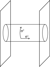
Figure 4: D-branes interacting via the tree-level exchange of a closed string.

To answer this question, we will have to study the tree-level interaction of two parallel D$p$-branes via the exchange of a closed string [12], depicted schematically in Fig. 4. For this interpretation time runs horizontally. However, if we take time to run vertically, then, the same diagram can be interpreted as a (one-loop) vacuum fluctuation of open strings with their end-points attached to the D-branes. In this second picture we can calculate this diagram to be

$${\cal A}=2V_{p+1}\int{d^{p+1}k\over(2\pi)^{p+1}}\int_{0}^{\infty}{dt\over 2t}e^{-2\pi\alpha^{\prime}tk^{2}-t{|Y|^{2}\over 2\pi\alpha^{\prime}}}{1\over\eta^{12}(it)}{1\over 2}\sum_{a,b}(-1)^{a+b+ab}\vartheta^{4}[^{a}_{b}](it)$$ (9.1)

$$=2V_{p+1}\int_{0}^{\infty}{dt\over 2t}(8\pi^{2}\alpha^{\prime}t)^{-{p+1\over 2}}e^{-t{|Y|^{2}\over 2\pi\alpha^{\prime}}}{1\over\eta^{12}(it)}{1\over 2}\sum_{a,b=0}^{1}(-1)^{a+b+ab}\vartheta^{4}[^{a}_{b}](it)\,.$$

$V_{p+1}$ is the world-volume of the $p$-brane, the factor of two is because of the two end-points, $|Y|^{2}$ is the distance between the D-branes. Of course the total result is zero, because of the $\vartheta$-identity. This reflects the fact that the D-branes are BPS states and exert no static force on each other. However, our purpose is to disentangle the contributions of the various intermediate massless states in the closed string channel. This can be obtained by taking the leading $t\to 0$ behavior of the integrand. In order to do this, we have to perform a modular transformation $t\to 1/t$ in the $\vartheta$- and $\eta$-functions. We obtain

$$\left.{\cal A}\right|^{\rm closed~{}~{}string}_{\rm massless}=8(1-1)V_{p+1}\int_{0}^{\infty}{dt\over t}(8\pi^{2}\alpha^{\prime}t)^{-{p+1\over 2}}~{}t^{4}~{}e^{-{t|Y|^{2}\over 2\pi\alpha^{\prime}}}$$ (9.2)

$$=2\pi(1-1)V_{p+1}(4\pi^{2}\alpha^{\prime})^{3-p}G_{9-p}(|Y|)$$

where

$$G_{d}(|Y|)={1\over 4\pi^{d/2}}\int_{0}^{\infty}{dt\over t^{(4-d)/2}}e^{-t|Y|^{2}}$$ (9.3)

is the massless scalar propagator in $d$ dimensions. The $(1-1)$ comes from the NS-NS and R-R sectors respectively. Now consider the RR forms coupled to p-branes with action

$$S={\alpha_{p}\over 2}\int F_{p+2}\;^{*}F_{p+2}+iT_{p}\int_{\rm branes}A_{p+1}\,,$$ (9.4)

with $F_{p+2}=dA_{p+1}$. Using this action, the same amplitude for exchange of $A_{p+1}$ between two D-branes at distance $|Y|$ in the transverse space of dimension $10-(p+1)=9-p$ is given by

$$\left.{\cal A}\right|_{\rm field~{}~{}theory}={(iT_{p})^{2}\over\alpha_{p}}V_{p+1}G_{9-p}(|Y|)\,,$$ (9.5)

where the factor of volume is there since the RR field can be absorbed or emitted at any point in the world-volume of the D-brane. Matching with the string calculation we obtain

$${T^{2}_{p}\over\alpha_{p}}=2\pi(4\pi^{2}\alpha^{\prime})^{3-p}\,.$$ (9.6)

We will now look at the DNT quantization condition which, with our normalization of the RR forms, and $D=10$ becomes

$${T_{p}T_{6-p}\over\alpha_{p}}=2\pi n\,.$$ (9.7)

From (9.6) we can verify directly that D-branes satisfy this quantization condition for the minimum quantum $n=1$!

Thus, we are led to accept that D-branes, with a nice (open) CFT description of their fluctuations, describe non-perturbative extended BPS states of the type-II string carrying non-trivial RR charge.

We will now describe a uniform normalization of the D-brane tensions. Our starting point is the type-IIA ten-dimensional effective action (6.1). The gravitational coupling $\kappa_{10}$ is given in terms of $\alpha^{\prime}$ as

$$2\kappa_{10}^{2}=(2\pi)^{7}\alpha^{\prime 4}\;\;.$$ (9.8)

We will also normalize all forms so that their kinetic terms are $(1/4\kappa_{10}^{2})\int d^{10}xF\otimes^{*}F$. This corresponds to $\alpha_{p}=1/(2\kappa_{10}^{2})$. We will define also the tensions of various p-branes via their world-volume action of the form

$$S_{p}=-T_{p}\int_{W_{p+1}}d^{p+1}\xi~{}e^{-\Phi/2}\sqrt{{\rm det}\hat{G}}-iT_{p}\int{}~{}A_{p+1}\;\;\;,$$ (9.9)

where $\hat{G}$ is the induced metric on the world-volume

$$\hat{G}_{\alpha\beta}=G_{\mu\nu}{\partial X^{\mu}\over\partial\xi^{\alpha}}{\partial X^{\nu}\over\partial\xi^{\beta}}$$ (9.10)

and

$$\int A_{p+1}={1\over(p+1)!}\int d^{p+1}\xi{}~{}A_{\mu_{1}\cdots\mu_{p+1}}{\partial X^{\mu_{1}}\over\partial\xi^{\alpha_{1}}}\cdots{\partial X^{\mu_{p+1}}\over\partial\xi^{\alpha_{p+1}}}\epsilon^{\alpha_{1}\cdots\alpha_{p+1}}\;\;.$$ (9.11)

The dilaton dependence will be explained in the next section. The DNT quantization condition in (9.7) becomes

$$2\kappa_{10}^{2}T_{p}T_{6-p}=2\pi n\;\;,$$ (9.12)

while (9.6) and (9.8) give

$$T_{p}={1\over(2\pi)^{p}(\alpha^{\prime})^{(p+1)/2}}\;\;.$$ (9.13)

We have obtained the IIA theory from the reduction of eleven-dimensional supergravity on a circle of volume $2\pi R_{11}=2\pi\sqrt{a^{\prime}}e^{\Phi/3}$. Consequently, the M-theory gravitational constant is

$$2\kappa_{11}^{2}=(2\pi)^{8}(\alpha^{\prime})^{9/2}\;\;.$$ (9.14)

The M-theory membrane, upon compactification of M-theory on a circle, becomes the type-IIA D2-brane. Thus, its tension $T^{M}_{2}$ should be equal to the D2-brane tension,

$$T^{M}_{2}=T_{2}={1\over(2\pi)^{2}(\alpha^{\prime})^{3/2}}\;\;.$$ (9.15)

Consider now the M-theory five-brane. It has a tension $T^{M}_{5}$ that can be computed from the DNT quantization condition

$$2\kappa_{11}^{2}T_{2}^{M}T^{M}_{5}=2\pi\;\;\;\to\;\;\;\;T^{M}_{5}={1\over(2\pi)^{5}(\alpha^{\prime})^{3}}\;.$$ (9.16)

On the other hand, wrapping one of the coordinates of the M5-brane around the circle should produce the D4-brane and we can confirm that

$$2\pi\sqrt{\alpha^{\prime}}T^{M}_{5}=T_{4}\;.$$ (9.17)

10 D-brane actions

We will now derive the massless fluctuations of a single Dp-brane. This parallels our detailed discussion of the type-I D1-brane. The difference here is that the open string fluctuations cannot have free ends. Thus, only the DD sector is relevant. Also there is no orientifold projection. In the NS sector, the massless bosonic states are a (p+1)-vector, $A_{\mu}$ corresponding to the state $b^{\mu}_{-1/2}|p\rangle$ and 9-p scalars, $X^{I}$ corresponding to the states $b^{I}_{-1/2}|p\rangle$. The $X^{I}$ represent the position coordinates of the Dp-brane in transverse space. These are the states we would obtain by reducing a ten-dimensional vector to p+1 dimensions. Similarly, from the R sector we obtain world-volume fermions which are the reduction of a ten-dimensional gaugino to (p+1) dimensions. In total we obtain the reduction of a ten-dimensional U(1) vector multiplet to p+1 dimensions. The world-volume supersymmetry has 16 conserved supercharges. Thus, the Dp-brane broke half-of the original supersymmetry as expected.

In order to calculate the world-volume action, we would have to calculate scattering of the massless states of the world-volume theory. The leading contribution comes from the disk diagram and is thus weighted with a factor of $e^{-\Phi/2}$. The calculation is similar with the calculation of the effective action in the ten-dimensional open oriented string theory. The result there is the Born-Infeld action for the gauge field [27]

$$S_{BI}=\int d^{10}x~{}e^{-\Phi/2}\sqrt{\det(\delta_{\mu\nu}+2\pi\alpha^{\prime}F_{\mu\nu})}\;\;.$$ (10.1)

Dimensionally reducing this action, we obtain the relevant Dp-brane action from the disk. There is a coupling to the spacetime background metric which gives the induced metric, (9.10). There is also a coupling to the spacetime NS antisymmetric tensor. This can be seen as follows. The closed string coupling to $B_{\mu\nu}$ and the vector $A_{\mu}$ can be summarized in

$$S_{B}={i\over 2\pi\alpha^{\prime}}\int_{M_{2}}d^{2}\xi~{}\epsilon^{\alpha\beta}B_{\mu\nu}\partial_{a}x^{\mu}\partial_{\beta}x^{\nu}-{i\over 2}\int_{B_{1}}ds~{}A_{\mu}\partial_{s}x^{\mu}\;\;,$$ (10.2)

where $M_{2}$ is the two-dimensional world-sheet with one-dimensional boundary $B_{1}$. Under a gauge transformation $\delta B_{\mu\nu}=\partial_{\mu}\Lambda_{\nu}-\partial_{\nu}\Lambda_{\mu}$, the action above changes by a boundary term,

$$\delta S_{B}={i\over\pi\alpha^{\prime}}\int_{B_{1}}ds~{}\Lambda_{\mu}\partial_{s}x^{\mu}\;\;.$$ (10.3)

To reinstate gauge invariance, the vector $A_{\mu}$ has to transform as $\delta A_{\mu}={1\over 2\pi\alpha^{\prime}}\Lambda_{\mu}$. Thus, the gauge invariant combination is

$${\cal F}_{\mu\nu}=2\pi\alpha^{\prime}F_{\mu\nu}-B_{\mu\nu}=2\pi\alpha^{\prime}(\partial_{\mu}A_{\nu}-\partial_{\nu}A_{\mu})-B_{\mu\nu}\;\;.$$ (10.4)

We can now sumarize the leading order Dp-brane action as

$$S_{p}=-T_{p}\int_{W_{p+1}}d^{p+1}\xi~{}e^{-\Phi/2}\sqrt{{\rm det}(\hat{G}+{\cal F})}-iT_{p}\int~{}A_{p+1}\;\;.$$ (10.5)

As we have seen in the previous section, the CP-odd term in the action comes from the next diagram, the annulus. There are however more CP-odd couplings coming from the annulus that involve q-forms with q$<$p. Their appearance is due to cancellation of anomalies, and we refer the reader to [28] for a detailed discussion. We will present here the result. It involves the roof-genus $\hat{I}_{1/2}(R)$ and the Chern character. Thus, (10.5) is extended to

$$S_{p}=-T_{p}\int_{W_{p+1}}d^{p+1}\xi~{}e^{-\Phi/2}\sqrt{{\rm det}(\hat{G}+{\cal F})}-iT_{p}\int~{}A\wedge Tr[e^{i{\cal F}/2\pi}]\sqrt{\hat{I}_{1/2}(R)}\;\;,$$ (10.6)

where $A$ stands for a formal sum of all RR forms, and the integration picks up the (p+1)-form in the sum.

As an example we will consider the action of the D1-string of type-IIB theory. The relevant forms that couple here is the RR two-form $B^{R}_{\mu\nu}$ as well as the RR scalar (zero-form) $S_{1}$. The action is

$$S_{1}=-{1\over 2\pi\alpha^{\prime}}\left[\int d^{2}\xi~{}{|S|\over\sqrt{S_{2}}}~{}\sqrt{{\rm det}(\hat{G}+{\cal F})}+i\int(B^{N}+{iS_{1}\over 2\pi}{\cal F})\right]\;\;,$$ (10.7)

where $e^{-\Phi/2}=S_{2}$. Note that ${|S|\over\sqrt{S_{2}}}=e^{-\Phi/2}$ when $S_{1}=0$.

We will now consider the effect of T-duality transformations on the Dp-branes. Consider the type-II theory with $x^{9}$ compactified on a circle of radius R. As we have mentioned earlier, the effect of a T-duality transformation on open strings is to interchange N and D boundary conditions. Consider first a Dp-brane not wrapping around the circle. This implies that one of its transverse coordinates (Dirichlet) is in the compact direction. Doing a T-duality transformation $R\to\alpha^{\prime}/R$, would change the boundary conditions along $X^{9}$ to Neumann and would produce a D(p+1)-brane wrapping around the circle of radius $\alpha^{\prime}/R$. Thus, the Dp-brane has been transformed into a D(p+1)-brane. The original Dp-brane action contains $T_{p}\int d^{p+1}\xi~{}e^{-\Phi/2}$. The dilaton transforms under duality as

$$e^{-\Phi/2}\to{\sqrt{\alpha^{\prime}}\over R}e^{-\Phi/2}\;\;.$$ (10.8)

Consequently, $T_{p}\sqrt{\alpha^{\prime}}/R=T_{p+1}(2\pi\alpha^{\prime}/R)$ and we obtain

$$T_{p+1}={T_{p}\over 2\pi\sqrt{\alpha^{\prime}}}\;\;,$$ (10.9)

which is in agreement with (9.13).

On the other hand, if the Dp-brane was wrapped around the compact direction, T-duality transforms it into a D(p-1)-brane. This action of T-duality on the various D-branes is a powerful tool for investigating non-perturbative physics due to them.

So far, we have discussed a single Dp-brane, interacting with the background type-II fields. An obvious question is: what happens when we have more than one parallel Dp-branes? Consider first the case where we have N Dp-branes being at the same point in transverse space. Then, the only difference in the previous analysis, is to include a Chan-Patton factor $i=1,2,\cdots,N$ at the open string end-points. We now have $N^{2}$ massless vector states, $b^{\mu}_{-1/2}|p;i,j\rangle$. Going through the same procedure as before, we will find that the massless fluctuations are described by the dimensional reduction of the ten-dimensional N=1 U(N) Yang-Mills multiplet on the world-volume of the brane (we have oriented open strings here). The U(1) factor of U(N) describes the overall center of mass of the system. If we take one of the Dp-branes and we separate it from the rest, the open strings stretching between it and the rest N-1 of the branes, acquire a mass-gap (non-trivial tension), and the massless vectors have a gauge group which is $\rm U(N-1)\times U(1)$. In terms of the world-sheet theory, this is an ordinary Higgs effect. For generic positions of the Dp-branes, the gauge group is $\rm U(1)^{N}$. The scalars that described the individual positions become now U(N) matrices. The world-volume action has a non-abelian generalization. In particular, to lowest order, it is the dimensional reduction of U(N) ten-dimensional Yang-Mills

$$S^{N}_{p}=-T_{p}Str\int_{W_{p+1}}d^{p+1}\xi~{}e^{-\Phi/2}(F_{\mu\nu}^{2}+2F_{\mu I}^{2}+F_{IJ}^{2})\;\;,$$ (10.10)

where

$$F_{\mu\nu}=\partial_{\mu}A_{\nu}-\partial_{\nu}A_{\mu}+[A_{\mu},A_{\nu}]\;\;,$$ (10.11)

$$F_{\mu I}=\partial_{\mu}X^{I}+[A_{\mu},X^{I}]\;\;\;,\;\;\;F_{IJ}=[X^{I},X^{J}]\;.$$ (10.12)

Both $A_{\mu}$ and $X^{I}$ are U(N) matrices. At the minimum of the potential, the matrices $X^{I}$ are commuting, and can be simultaneously diagonalized. Their eigenvalues can be interpreted as the coordinates of the N Dp-branes.

One very interesting application of D-branes is the following. D-branes wrapped around compact manifolds produce point-like RR charged particles in lower dimensions. Such particles have an effective description as microscopic black holes. Using D-brane techniques, their multiplicity can be computed for fixed charge and mass. It can be shown that this multiplicity agrees to leading order with the Bekenstein-Hawking entropy formula for classical black holes [29]. The interested reader may consult [30] for a review.

11 Heterotic/Type-II duality in six and four Dimensions

There is another non-trivial duality relation that we are going to discuss in some detail: that of the heterotic string compactified to six dimensions on $T^{4}$ and the type-IIA string compactified on K3. Both theories have N=2 supersymmetry in six dimensions. Both theories have the same massless spectrum, containing the N=2 supergravity multiplet and twenty vector multiplets.

The six-dimensional tree-level heterotic effective action in the $\sigma$-model frame is

$$S^{\rm heterotic}_{D}=\int~{}d^{D}x~{}\sqrt{-{\rm det}~{}G}e^{-\Phi}\left[R+\partial^{\mu}\Phi\partial_{\mu}\Phi-{1\over 12}\hat{H}^{\mu\nu\rho}\hat{H}_{\mu\nu\rho}-\right.$$ (11.1)

$$\left.-{1\over 4}(\hat{M}^{-1})_{ij}F^{i}_{\mu\nu}F^{j\mu\nu}+{1\over 8}Tr(\partial_{\mu}\hat{M}\partial^{\mu}\hat{M}^{-1})\right]\,,$$

where $i=1,2,\dots,36-2D$ and

$$\hat{H}_{\mu\nu\rho}=\partial_{\mu}B_{\nu\rho}-{1\over 2}L_{ij}A^{i}_{\mu}F^{j}_{\nu\rho}+{\rm cyclic}\,.$$ (11.2)

The moduli scalar matrix $\hat{M}$ is,

$$M=\left(\matrix{G^{-1}&G^{-1}C&G^{-1}Y^{t}\cr C^{t}G^{-1}&G+C^{t}G^{-1}C+Y^{t}Y&C^{t}G^{-1}Y^{t}+Y^{t}\cr YG^{-1}&YG^{-1}C+Y&{\bf 1}_{16}+YG^{-1}Y^{t}\cr}\right)\,,$$ (11.3)

where ${\bf 1}_{16}$ is the sixteen-dimensional unit matrix and

$$C_{\alpha\beta}=B_{\alpha\beta}-{1\over 2}Y^{I}_{\alpha}Y^{I}_{\beta}\,.$$ (11.4)

Going to the Einstein frame by $G_{\mu\nu}\to e^{\Phi/2}G_{\mu\nu}$, we obtain

$$S^{\rm het}_{D=6}=\int~{}d^{6}x~{}\sqrt{-G}\left[R-{1\over 4}\partial^{\mu}\Phi\partial_{\mu}\Phi-{e^{-\Phi}\over 12}\hat{H}^{\mu\nu\rho}\hat{H}_{\mu\nu\rho}-\right.$$ (11.5)

$$\left.-{e^{-{\Phi\over 2}}\over 4}(\hat{M}^{-1})_{ij}F^{i}_{\mu\nu}F^{j\mu\nu}+{1\over 8}Tr(\partial_{\mu}\hat{M}\partial^{\mu}\hat{M}^{-1})\right]\,.$$

The tree-level type-IIA effective action in the $\sigma$-model frame is

$$S^{IIA}_{K3}=\int d^{6}x\sqrt{-{\rm det}~{}G_{6}}e^{-\Phi}\left[R+\nabla^{\mu}\Phi\nabla_{\mu}\Phi-{1\over 12}H^{\mu\nu\rho}H_{\mu\nu\rho}+\right.$$ (11.6)

$$\left.+{1\over 8}Tr(\partial_{\mu}\hat{M}\partial^{\mu}\hat{M}^{-1})\right]-{1\over 4}\int d^{6}x\sqrt{-{\rm det}~{}G}(\hat{M}^{-1})_{IJ}F^{I}_{\mu\nu}F^{J\mu\nu}+{1\over 16}\int d^{6}x\epsilon^{\mu\nu\rho\sigma\tau\upsilon}B_{\mu\nu}F^{I}_{\rho\sigma}\hat{L}_{IJ}F^{J}_{\tau\upsilon}\,,$$

where $I=1,2,\dots,24$.

Going again to the Einstein frame we obtain

$$S^{IIA}_{D=6}=\int d^{6}x\sqrt{-G}\left[R-{1\over 4}\partial^{\mu}\Phi\partial_{\mu}\Phi-{1\over 12}e^{-\Phi}H^{\mu\nu\rho}H_{\mu\nu\rho}-\right.$$ (11.7)

$$\left.-{1\over 4}e^{\Phi/2}(\hat{M}^{-1})_{ij}F^{i}_{\mu\nu}F^{j\mu\nu}+{1\over 8}Tr(\partial_{\mu}\hat{M}\partial^{\mu}\hat{M}^{-1})\right]+{1\over 16}\int d^{6}x\epsilon^{\mu\nu\rho\sigma\tau\varepsilon}B_{\mu\nu}F^{i}_{\rho\sigma}\hat{L}_{ij}F^{j}_{\tau\varepsilon}\;,$$

where $\hat{L}$ is the O(4,20) invariant metric. Notice the following differences: The heterotic $\hat{H}_{\mu\nu\rho}$ contains the Chern-Simons term (11.2) while the type-IIA one doesn’t. The type-IIA action instead contains a parity-odd term coupling the gauge fields and $B_{\mu\nu}$. Both effective actions have a continuous O(4,20,ℝ) symmetry which is broken in the string theory to the T-duality group O(4,20,ℤ).

We will denote by a prime the fields of the type-IIA theory (Einstein frame) and without a prime those of the heterotic theory.

Exercise. Derive the equations of motion stemming from the actions (11.5) and (11.7). Show that the two sets of equations of motion are equivalent via the following (duality) transformations

$$\Phi^{\prime}=-\Phi\;\;\;,\;\;\;G^{\prime}_{\mu\nu}=G_{\mu\nu}\;\;\;,\;\;\;\hat{M}^{\prime}=\hat{M}\;\;\;,\;\;\;A^{\prime i}_{\mu}=A^{i}_{\mu}\,,$$ (11.8)

$$e^{-\Phi}\hat{H}_{\mu\nu\rho}={1\over 6}{{\epsilon_{\mu\nu\rho}}^{\sigma\tau\varepsilon}\over\sqrt{-G}}H^{\prime}_{\sigma\tau\varepsilon}\,,$$ (11.9)

where the data on the right-hand side are evaluated in the type-IIA theory.

There is a way to see some indication of this duality by considering the compactification of M-theory on $S^{1}\times$K3 which is equivalent to type-IIA on K3. As we have seen in a previous section, all vectors descend from the RR one- and three-forms of the ten-dimensional type-IIA theory, and these descend from the three-form of M-theory to which the membrane and five-brane couple. The membrane wrapped around $S^{1}$ would give a string in six dimensions. Like in ten dimensions, this is the perturbative type-IIA string. There is another string however, obtained by wrapping the five-brane around the whole K3. This is the heterotic string [31].

There is further evidence for this duality. The effective action of type-IIA theory on K3 has a string solution singular at the core. The zero mode structure of the string is similar to the perturbative type-IIA string. There is also a string solution which is regular at the core. This is a solitonic string and analysis of its zero modes indicates that it has the same (chiral) word-sheet structure as the heterotic string. The string-string duality map (11.8-11.9) exchanges the roles of the two strings. The type-IIA string now becomes regular (solitonic), while the heterotic string solution becomes singular.

We will now compactify further both theories on a two-torus down to four dimensions and examine the consequences of the duality. In both cases we use the standard Kaluza-Klein ansatz described in Appendix A. The four-dimensional dilaton becomes as usual

$$\phi=\Phi-{1\over 2}\log[\det G_{\alpha\beta}]\,,$$ (11.10)

where $G_{\alpha\beta}$ is the metric of $T^{2}$ and $B_{\alpha\beta}=\epsilon_{\alpha\beta}B$ is the antisymmetric tensor. We obtain

$$S_{D=4}^{het}=\int d^{4}x\sqrt{-g}e^{-\phi}\left[R+L_{B}+L_{\rm gauge}+L_{\rm scalar}\right]\,,$$ (11.11)

where

$$L_{g+\phi}=R+\partial^{\mu}\phi\partial_{\mu}\phi\,,$$ (11.12)

$$L_{B}=-{1\over 12}H^{\mu\nu\rho}H_{\mu\nu\rho}\,,$$ (11.13)

with

$$H_{\mu\nu\rho}=\partial_{\mu}B_{\nu\rho}-{1\over 2}\left[B_{\mu\alpha}F^{A,\alpha}_{\nu\rho}+A^{\alpha}_{\mu}F^{B}_{a,\nu\rho}+\hat{L}_{ij}A^{i}_{\mu}F^{j}_{\nu\rho}\right]+{\rm cyclic}$$ (11.14)

$$\equiv\partial_{\mu}B_{\nu\rho}-{1\over 2}L_{IJ}A^{I}_{\mu}F^{J}_{\nu\rho}+{\rm cyclic}\,.$$

The matrix

$$L=\left(\matrix{0&0&1&0&{\vec{0}}\cr 0&0&0&1&\vec{0}\cr 1&0&0&0&\vec{0}\cr 0&1&0&0&\vec{0}\cr\vec{0}&\vec{0}&\vec{0}&\vec{0}&\hat{L}\cr}\right)$$ (11.15)

is the O(6,22) invariant metric. Also

$$C_{\alpha\beta}=\epsilon_{\alpha\beta}B-{1\over 2}\hat{L}_{ij}Y^{i}_{\alpha}Y^{j}_{\beta}\,,$$ (11.16)

so that

$$L_{\rm gauge}=-{1\over 4}\left\{\left[(\hat{M}^{-1})_{ij}+\hat{L}_{ki}\hat{L}_{lj}Y^{k}_{\alpha}G^{\alpha\beta}Y^{l}_{\beta}\right]\;\;F^{i}_{\mu\nu}F^{j,\mu\nu}+G^{\alpha\beta}\;\;F^{B}_{\alpha,\mu\nu}F_{B,\beta}^{\mu\nu}+\right.$$

$$+\left[G_{\alpha\beta}+C_{\gamma\alpha}G^{\gamma\delta}C_{\delta\beta}+Y^{i}_{\alpha}(\hat{M}^{-1})_{ij}Y^{j}_{\beta}\right]\;\;F^{A,a}_{\mu\nu}F_{A}^{\beta,\mu\nu}-2G^{\alpha\gamma}C_{\gamma\beta}\;\;F^{B}_{\alpha,\mu\nu}F^{A,\beta,\mu\nu}-$$ (11.17)

$$\left.-2\hat{L}_{ij}Y^{i}_{\alpha}G^{\alpha\beta}\;\;F^{j}_{\mu\nu}F^{B,\mu\nu}_{\beta}+2(Y^{i}_{\alpha}(\hat{M}^{-1})_{ij}+C_{\gamma\alpha}G^{\gamma\beta}\hat{L}_{ij}Y^{i}_{\beta})\;\;F^{a,A}_{\mu\nu}F^{j,\mu\nu}\right\}$$

$$\equiv-{1\over 4}(M^{-1})_{IJ}F^{I}_{\mu\nu}F^{J,\mu\nu}\;\;,$$

where the index I takes 28 values. For the scalars

$$L_{\rm scalar}=\partial_{\mu}\phi\partial^{\mu}\phi+{1\over 8}Tr[\partial_{\mu}\hat{M}\partial^{\mu}\hat{M}^{-1}]-{1\over 2}G^{\alpha\beta}(\hat{M}^{-1})_{ij}\partial_{\mu}Y^{i}_{\alpha}\partial^{\mu}Y^{j}_{\beta}+$$

$$+{1\over 4}\partial_{\mu}G_{\alpha\beta}\partial^{\mu}G^{\alpha\beta}-{1\over 2detG}\left[\partial_{\mu}B+\epsilon^{\alpha\beta}\hat{L}_{ij}Y^{i}_{\alpha}\partial_{\mu}Y^{j}_{\beta}\right]\left[\partial^{\mu}B+\epsilon^{\alpha\beta}\hat{L}_{ij}Y^{i}_{\alpha}\partial^{\mu}Y^{j}_{\beta}\right]$$ (11.18)

$$=\partial_{\mu}\phi\partial^{\mu}\phi+{1\over 8}Tr[\partial_{\mu}M\partial^{\mu}M^{-1}]\,.$$

We will now go to the standard axion basis in terms of the usual duality transformation in four dimensions. First we will go to the Einstein frame by

$$g_{\mu\nu}\to e^{-\phi}g_{\mu\nu}\,,$$ (11.19)

so that the action becomes

$$S^{het,E}_{D=4}=\int d^{4}x\sqrt{-g}\;\left[R-{1\over 2}\partial^{\mu}\phi\partial_{\mu}\phi-{1\over 12}e^{-2\phi}H^{\mu\nu\rho}H_{\mu\nu\rho}-\right.$$ (11.20)

$$\left.-{1\over 4}e^{-\phi}(M^{-1})_{IJ}F^{I}_{\mu\nu}F^{J,\mu\nu}+{1\over 8}Tr(\partial_{\mu}M\partial^{\mu}M^{-1})\right]\,.$$

The axion is introduced as usual,

$$e^{-2\phi}H_{\mu\nu\rho}={{\epsilon_{\mu\nu\rho}}^{\sigma}\over\sqrt{-g}}\partial_{\sigma}a\,.$$ (11.21)

The transformed equations come from the following action:

$$\tilde{S}^{het}_{D=4}=\int d^{4}x\sqrt{-g}\;\left[R-{1\over 2}\partial^{\mu}\phi\partial_{\mu}\phi-{1\over 2}e^{2\phi}\partial^{\mu}a\partial_{\mu}a-{1\over 4}e^{-\phi}(M^{-1})_{IJ}F^{I}_{\mu\nu}F^{J,\mu\nu}\right.$$ (11.22)

$$\left.+{1\over 4}a\;L_{IJ}F^{I}_{\mu\nu}\tilde{F}^{J,\mu\nu}+{1\over 8}Tr(\partial_{\mu}M\partial^{\mu}M^{-1})\right]\;\;,$$

where

$$\tilde{F}^{\mu\nu}={1\over 2}{\epsilon^{\mu\nu\rho\sigma}\over\sqrt{-g}}F_{\rho\sigma}\,.$$ (11.23)

Finally, defining the complex S field

$$S=a+i\;e^{-\phi}\,,$$ (11.24)

we obtain

$$\tilde{S}^{het}_{D=4}=\int d^{4}x\sqrt{-g}\;\left[R-{1\over 2}{\partial^{\mu}S\partial_{\mu}\bar{S}\over{\rm Im}S^{2}}-{1\over 4}{\rm Im}S(M^{-1})_{IJ}F^{I}_{\mu\nu}F^{J,\mu\nu}\right.$$ (11.25)

$$\left.+{1\over 4}{\rm Re}S\;L_{IJ}F^{I}_{\mu\nu}\tilde{F}^{J,\mu\nu}+{1\over 8}Tr(\partial_{\mu}M\partial^{\mu}M^{-1})\right]\,.$$

Now consider the type-IIA action (11.6). Going through the same procedure and introducing the axion via

$$e^{-2\phi}H_{\mu\nu\rho}={{\epsilon_{\mu\nu\rho}}^{\sigma}\over\sqrt{-g}}\left[\partial_{\sigma}a+{1\over 2}\hat{L}_{ij}Y^{i}_{\alpha}\delta_{\sigma}Y^{j}_{\beta}\epsilon^{\alpha\beta}\right]\,,$$ (11.26)

we obtain the following four-dimensional action in the Einstein frame

$$\tilde{S}_{D=4}^{IIA}=\int d^{4}x\sqrt{-g}\left[R+L^{\rm even}_{\rm gauge}+L^{\rm odd}_{\rm gauge}+L_{\rm scalar}\right]\,,$$ (11.27)

with

$$L^{\rm even}_{\rm gauge}=-{1\over 4}\int d^{4}x\sqrt{-g}\left[e^{-\phi}G^{\alpha\beta}\left(F^{B}_{\alpha,\mu\nu}-B_{\alpha\gamma}F^{A,\gamma}_{\mu\nu}\right)\left(F^{B,\mu\nu}_{\beta}-B_{\alpha\delta}F^{\delta,\mu\nu}_{A}\right)+\right.$$ (11.28)

$$\left.+e^{-\phi}G_{\alpha\beta}F^{A,\alpha}_{\mu\nu}F^{\beta,\mu\nu}_{A}+\sqrt{{\rm det}G_{\alpha\beta}}(\hat{M}^{-1})_{ij}\left(F^{i}_{\mu\nu}+Y^{i}_{\alpha}F^{A,\alpha}_{\mu\nu}\right)\left(F^{j,\mu\nu}+Y^{j}_{\beta}F^{\beta,\mu\nu}_{A}\right)\right]\,,$$

$$L^{\rm odd}_{\rm gauge}={1\over 2}\int d^{4}x\epsilon^{\mu\nu\rho\sigma}\left[{1\over 4}aF^{B}_{\alpha,\mu\nu}F^{A,\alpha}_{\rho\sigma}+{1\over 2}\epsilon^{\alpha\beta}\hat{L}_{ij}Y^{i}_{\beta}F^{B}_{\alpha,\mu\nu}\left(F^{j}_{\rho\sigma}+{1\over 2}Y^{j}_{\gamma}F^{A,\gamma}_{\rho\sigma}\right)\right.$$ (11.29)

$$\left.-{1\over 8}\epsilon^{\alpha\beta}\hat{L}_{ij}B_{\alpha\beta}\left(F^{i}_{\mu\nu}+Y^{i}_{\gamma}F^{A,\gamma}_{\mu\nu}\right)\left(F^{j}_{\rho\sigma}+Y^{j}_{\delta}F^{A,\delta}_{\rho\sigma}\right)\right]$$

,

$$L_{\rm scalar}=-{1\over 2}(\partial\phi)^{2}+{1\over 4}\partial^{\mu}G_{\alpha\beta}\partial_{\mu}G^{\alpha\beta}-{1\over 2detG}\partial_{\mu}B\partial^{\mu}B+{1\over 8}Tr[\partial_{\mu}\hat{M}\partial^{\mu}\hat{M}^{-1}]+$$ (11.30)

$$-{1\over 2}e^{2\phi}(\partial_{\mu}a+{1\over 2}\hat{L}_{ij}\epsilon^{\alpha\beta}Y^{i}_{\alpha}\partial^{\mu}Y^{j}_{\beta})^{2}-{1\over 2}e^{\phi}\sqrt{{\rm det}G_{\alpha\beta}}(\hat{M}^{-1})_{ij}G^{\alpha\beta}\partial_{\mu}Y^{i}_{\alpha}\partial^{\mu}Y^{j}_{\beta}\,.$$

Now we will use unprimed fields to refer to the heterotic side and primed ones for the type-II side. We will now work out the implications of the six-dimensional duality relations (11.8,11.9) in four dimensions. From (11.8), we obtain

$$e^{-\phi}=\sqrt{{\rm det}G^{\prime}_{\alpha\beta}}\;\;\;,\;\;\;e^{-\phi^{\prime}}=\sqrt{{\rm det}G_{\alpha\beta}}\,,$$ (11.31)

$${G_{\alpha\beta}\over\sqrt{{\rm det}G_{\alpha\beta}}}={G^{\prime}_{\alpha\beta}\over\sqrt{{\rm det}G^{\prime}_{\alpha\beta}}}\;\;\;,\;\;\;A^{\prime\alpha}_{\mu}=A^{\alpha}_{\mu}\,,$$ (11.32)

$$g_{\mu\nu}=g^{\prime}_{\mu\nu}\;\;\;\;\;{\rm Einstein~{}~{}frame}\,,$$ (11.33)

$$\hat{M}^{\prime}=\hat{M}\;\;\;,\;\;\;A^{i}_{\mu}=A^{\prime i}_{\mu}\;\;\;,\;\;\;Y^{i}_{\alpha}=Y^{\prime i}_{\alpha}\,.$$ (11.34)

Finally, the relation (11.9) implies

$$A=B^{\prime}\;\;\;,\;\;\;A^{\prime}=B$$ (11.35)

and

$${1\over 2}{{\epsilon_{\mu\nu}}^{\rho\sigma}\over\sqrt{-g}}\epsilon^{\alpha\beta}F^{B^{\prime}}_{\beta,\rho\sigma}=e^{-\phi}G^{\alpha\beta}\left[F^{B}_{\beta,\mu\nu}-C_{\beta\gamma}F^{A,\gamma}_{\mu\nu}-\hat{L}_{ij}Y^{i}_{\beta}F^{j}_{\mu\nu}\right]-{1\over 2}a{{\epsilon_{\mu\nu}}^{\rho\sigma}\over\sqrt{-g}}F^{A,\alpha}_{\rho\sigma}\,,$$ (11.36)

which is an electric-magnetic duality transformation on the $B_{\alpha,\mu}$ gauge fields (see Appendix D). It is easy to check that this duality maps the scalar heterotic terms to the type-IIA ones and vice versa.

In the following, we will keep the 4 moduli of the two torus and the 16 Wilson lines $Y^{i}_{\alpha}$ In the heterotic case we will define the $T,U$ moduli of the torus and the complex Wilson lines as

$$W^{i}=W^{i}_{1}+iW_{2}^{i}=-Y^{i}_{2}+UY^{i}_{1}\,,$$ (11.37)

$$G_{\alpha\beta}={T_{2}-{\sum_{i}(W^{i}_{2})^{2}\over 2U_{2}}\over U_{2}}\left(\matrix{1&U_{1}\cr U_{1}&|U|^{2}\cr}\right)\;\;\;,\;\;\;B=T_{1}-{\sum_{i}W_{1}^{i}W_{2}^{i}\over 2U_{2}}\,.$$ (11.38)

Altogether we have the complex field S$\in$SU(1,1)/U(1) (11.24) and the $T,U,W^{i}$ moduli $\in$ ${{\rm O(2,18)}\over{\rm O(2)\times O(18)}}$. Then the relevant scalar kinetic terms can be written as

$$L^{het}_{\rm scalar}=-{1\over 2}\partial_{z^{i}}\partial_{\bar{z}^{j}}K(z_{k},\bar{z}_{k})~{}\partial_{\mu}z^{i}\partial^{\mu}\bar{z}^{j}\,,$$ (11.39)

where the Kähler potential is

$$K=\log\left[S_{2}\left(T_{2}U_{2}-{1\over 2}\sum_{i}(W_{2}^{i})^{2}\right)\right]\,.$$ (11.40)

In the type-IIA case the complex structure is different: (11.37) remains the same but

$$G_{\alpha\beta}={T_{2}\over U_{2}}\left(\matrix{1&U_{1}\cr U_{1}&|U|^{2}\cr}\right)\;\;\;,\;\;\;B=T_{1}\,.$$ (11.41)

Also

$$S=a-{\sum_{i}W_{1}^{i}W_{2}^{i}\over 2U_{2}}+i(e^{-\phi}-{\sum_{i}(W^{i}_{2})^{2}\over 2U_{2}})\,.$$ (11.42)

Here $T\in$SU(1,1)/U(1) and $S,U,W^{i}\in{{\rm O(2,18)\over O(2)\times O(18)}}$. In this language the duality transformations become

$$S^{\prime}=T\;\;\;,\;\;\;T^{\prime}=S\;\;\;,\;\;\;U=U^{\prime}\;\;\;,\;\;\;W^{i}=W^{\prime i}\,.$$ (11.43)

In the type-IIA string, there is a SL(2,$\hbox{\mybb Z})$ $T$-duality symmetry acting on T by fractional transformations. This is a good symmetry in perturbation theory. We also expect it to be a good symmetry non-perturbatively, since it is a discrete remnant of a gauge symmetry and is not expected to be broken by non-perturbative effects. Then heterotic/type-II duality implies that there is an SL(2,$\hbox{\mybb Z})$ S-symmetry that acts on the coupling constant and the axion. This is a non-perturbative symmetry from the point of view of the heterotic string. It acts as an electric magnetic duality on all the 28 gauge fields. In the field theory limit it implies an S-duality symmetry for N=4 super Yang-Mills theory in four dimensions.

We will finally see how heterotic/type-II duality acts on the 28 electric and 28 magnetic charges. Label the electric charges by a vector ($m_{1},m_{2},n_{1},n_{2},q^{i}$) where $m_{i}$ are the momenta of the two torus, $n_{i}$ are the respective winding numbers, and $q^{i}$ are the rest of the 24 charges. For the magnetic charges we write the vector ($\tilde{m}_{1},\tilde{m}_{2},\tilde{n}_{1},\tilde{n}_{2},\tilde{q}^{i}$). Because of (11.36) we have the following duality map.

$$\left(\matrix{m_{1}\cr m_{2}\cr n_{1}\cr n_{2}\cr q^{i}\cr}\right)\to\left(\matrix{m_{1}\cr m_{2}\cr\tilde{n}_{2}\cr-\tilde{n}_{1}\cr q^{i}\cr}\right)\;\;,\;\;\left(\matrix{\tilde{m}_{1}\cr\tilde{m}_{2}\cr\tilde{n}_{1}\cr\tilde{n}_{2}\cr\tilde{q}^{i}\cr}\right)\to\left(\matrix{\tilde{m}_{1}\cr\tilde{m}_{2}\cr-n_{2}\cr n_{1}\cr\tilde{q}^{i}\cr}\right)\,.$$ (11.44)

One can compute the spectrum of BPS multiplets both short and intermediate. The results of section 12 are useful in this respect.

Exercise. Find the BPS multiplicities on the heterotic and type-IIA side in four dimensions.

There are indirect quantitative tests of this duality. Compactifying the heterotic string to four dimensions with N=2 supersymmetry can be dual to the type-IIA string compactified on a CY manifold of a special kind (K3 fibration over $P^{1}$) [32, 33, 34]. In the heterotic theory, the dilaton is in a vector multiplet. Consequently, the vector multiplet moduli space has perturbative and non-perturbative corrections while the hypermultiplet moduli space is exact. In the dual type-II theory, the dilaton is in a hypermultiplet. Consequently, the vector moduli space geometry has no corrections and can be computed at tree-level. Doing the duality map that should reproduce all quantum corrections to the heterotic side. This has been done in some examples, and in this way the one-loop heterotic correction was obtained which agreed with the heterotic computation. Moreover, all instanton effects were obtained this way. Taking the field theory limit and decoupling gravity, the Seiberg-Witten solution was verified for N=2 gauge theory. This procedure gives also a geometric interpretation of the Seiberg-Witten solution. A review of these developements can be found in [35].

12 Helicity string partition functions and multiplicities of BPS states

We have seen in section 3 that BPS states are important ingredients in non-perturbative dualities. The reason is that their special properties, most of the time, guarantee that such states survive at strong coupling. In this section we would like to analyze ways of counting BPS states in string perturbation theory.

An important point that should be stressed from the beginning is the following: A generic BPS state $is$ $not$ protected from quantum corrections. The reason is that sometimes groups of short BPS multiplets can combine into long multiplets of supersymmetry. Such long multiplets are not protected from non-renormalization theorems. We would like thus to count BPS multiplicities in such a way that only “unpaired” multiplets contribute. As it is explained in Appendix B, this can be done with the help of helicity supertrace formulae. They have precisely the properties we need in order to count BPS multiplicities that are protected from non-renormalization theorems. Moreover, multiplicities counted via helicity supertraces are insensitive to moduli. They are the generalizations of the elliptic genus which is the stringy generalization of the Dirac index. In this sense, they are indices, insensitive to the details of the physics. We will show here how we can compute helicity supertraces in perturbative string groundstates and we will work out some interesting examples.

We will introduce the helicity generating partition functions for $D=4$ string theories with $N\geq 1$ spacetime supersymmetry. The physical helicity in closed string theory $\lambda$ is a sum of the left helicity $\lambda_{L}$ coming from the left movers and the right helicity $\lambda_{R}$ coming from the right movers. Then, we can consider the following helicity-generating partition function

$$Z(v,\bar{v})=Str[q^{L_{0}}\;\bar{q}^{\bar{L}_{0}}e^{2\pi iv\lambda_{R}-2\pi i\bar{v}\lambda_{L}}]\,.$$ (12.1)

We will first examine the heterotic string. Four-dimensional vacua with at least N=1 spacetime supersymmetry have the following partition function

$$Z^{\rm heterotic}_{D=4}={1\over\tau_{2}\eta^{2}\bar{\eta}^{2}}\sum_{a,b=0}^{1}{}~{}(-1)^{a+b+ab}~{}{\vartheta[^{a}_{b}]\over\eta}~{}C^{Int}[^{a}_{b}]\,,$$ (12.2)

where we have separated the (light-cone) bosonic and fermionic contributions of the four-dimensional part. $C[^{a}_{b}]$ is the partition function of the internal CFT with $(c,\bar{c})=(9,22)$ and at least (2,0) superconformal symmetry. $a=0$ corresponds to the NS sector, $a=1$ to the R sector and $b=0,1$ indicates the presence of the projection $(-1)^{F_{L}}$, where $F_{L}$ is the zero mode of the N=2, U(1) current.

The oscillators that would contribute to the left helicity are the left moving light-cone bosons $\partial X^{\pm}=\partial X^{3}\pm i\partial X^{4}$ contributing helicity $\pm 1$ respectively, and the the light-cone fermions $\psi^{\pm}$ contributing again $\pm 1$ to the left helicity. Only $\bar{\partial}X^{\pm}$ contribute to the right-moving helicity. Calculating (12.1) is straightforward with the result

$$Z^{\rm heterotic}_{D=4}(v,\bar{v})={\xi(v)\bar{\xi}(\bar{v})\over\tau_{2}\eta^{2}\bar{\eta}^{2}}\sum_{a,b=0}^{1}{}~{}(-1)^{a+b+ab}~{}{\vartheta[^{a}_{b}](v)\over\eta}~{}C^{Int}[^{a}_{b}]\,,$$ (12.3)

where $\xi(v)$ is given in (C.15). This can be simplified using spacetime supersymmetry to

$$Z^{\rm heterotic}_{D=4}(v,\bar{v})={\xi(v)\bar{\xi}(\bar{v})\over\tau_{2}\eta^{2}\bar{\eta}^{2}}{\vartheta[^{1}_{1}](v/2)\over\eta}~{}C^{Int}[^{1}_{1}](v/2)\,,$$ (12.4)

with

$$C^{Int}[^{1}_{1}](v)=Tr_{R}[(-1)^{F^{Int}}~{}e^{2\pi iv~{}J_{0}}~{}q^{L_{0}^{Int}-{3/8}}{}~{}\bar{q}^{\bar{L}_{0}^{Int}-11/12}]\,,$$ (12.5)

where the trace is in the Ramond sector, and $J_{0}$ is the zero mode of the U(1) current of the N=2 superconformal algebra. $C^{Int}[^{1}_{1}](v)$ is the elliptic genus of the internal (2,0) theory and is antiholomorphic. The leading term of $C^{Int}[^{1}_{1}](0)$ coincides with the Euler number in CY compactifications.

If we define

$$Q={1\over 2\pi i}{\partial\over\partial v}\;\;\;,\;\;\;\bar{Q}=-{1\over 2\pi i}{\partial\over\partial\bar{v}}\,,$$ (12.6)

then the helicity supertraces can be written as

$$Str[\lambda^{2n}]=\left.(Q+\bar{Q})^{2n}\;Z^{\rm heterotic}_{D=4}(v,\bar{v})\right|_{v=\bar{v}=0}\,.$$ (12.7)

Consider as an example the heterotic string on $T^{6}$ with N=4, $D=4$ spacetime supersymmetry. Its helicity partition function is

$$Z^{\rm heterotic}_{N=4}(v,\bar{v})={\vartheta^{4}_{1}(v/2)\over\eta^{12}\bar{\eta}^{24}}\xi(v)\bar{\xi}(\bar{v}){\Gamma_{6,22}\over\tau_{2}}\,.$$ (12.8)

It is obvious that we need at least four powers of $Q$ in order to get a non-vanishing contribution, implying $B_{0}=B_{2}=0$, in agreement with the N=4 supertrace formulae derived in Appendix B. We will calculate $B_{4}$ which, according to (B.33),(B.34) is sensitive to short multiplets only:

$$B_{4}=\langle(Q+\bar{Q})^{4}\rangle=\langle Q^{4}\rangle={3\over 2}{1\over\bar{\eta}^{24}}\,.$$ (12.9)

For the massless states the result agrees with (B.34), as it should. Moreover, from (B.33) we observe that massive short multiplets with a bosonic ground-state give an opposite contribution from multiplets with a fermionic ground-state. We learn that all such short massive multiplets in the heterotic spectrum are ”bosonic” with multiplicities given by the coefficients of the $\eta^{-24}$.

Consider further

$$B_{6}=\langle(Q+\bar{Q})^{6}\rangle=\langle Q^{6}+15Q^{4}\bar{Q}^{2}\rangle={15\over 8}{2-\bar{E}_{2}\over\bar{\eta}^{24}}\,.$$ (12.10)

Since there can be no intermediate multiplets in the perturbative heterotic spectrum we get only contributions from the short multiplets. An explicit analysis at low levels confirms the agreement between (B.33) and (12.10).

For type-II vacua, there are fermionic contributions to the helicity both from the left-moving and right-moving world-sheet fermions. We will consider as a first example the type-II string, compactified on $T^{6}$ to four dimensions with maximal N=8 supersymmetry.

The light-cone helicity generating partition function is

$$Z^{II}_{N=8}(v,\bar{v})=Str[q^{L_{0}}\;\bar{q}^{\bar{L}_{0}}e^{2\pi iv\lambda_{R}-2\pi i\bar{v}\lambda_{L}}]=$$ (12.11)

$$={1\over 4}\sum_{\alpha,\beta=0}^{1}\sum_{\bar{\alpha},\bar{\beta}=0}^{1}\;(-1)^{\alpha+\beta+\alpha\beta}{\vartheta[^{\alpha}_{\beta}](v)\vartheta^{3}[^{\alpha}_{\beta}](0)\over\eta^{4}}\;\;(-1)^{\bar{\alpha}+\bar{\beta}+\bar{\alpha}\bar{\beta}}{\bar{\vartheta}[^{\bar{\alpha}}_{\bar{\beta}}]\bar{\vartheta}^{3}[^{\bar{\alpha}}_{\bar{\beta}}](0)\over\bar{\eta}^{4}}\;\;{\xi(v)\bar{\xi}(\bar{v})\over{\rm Im}\tau|\eta|^{4}}\;\;{\Gamma_{6,6}\over|\eta|^{12}}=$$

$$={\Gamma_{6,6}\over{\rm Im}\tau}\;\;{\vartheta_{1}^{4}(v/2)\over\eta^{12}}{\bar{\vartheta}_{1}^{4}(\bar{v}/2)\over\bar{\eta}^{12}}\;\;\xi(v)\bar{\xi}(\bar{v})\;\;.$$

It is obvious that in order to obtain a non-zero result, we need at least a $Q^{4}$ on the left and a $\bar{Q}^{4}$ on the right. This is in agreement with our statement in appendix B: $B_{0}=B_{2}=B_{4}=B_{6}=0$ for an $N=8$ theory. The first non-trivial case is $B_{8}$ and by straightforward computation we obtain

$$B_{8}\equiv Str[\lambda^{8}]=\langle(Q+\bar{Q})^{8}\rangle=70\langle Q^{4}\bar{Q}^{4}\rangle={315\over 2}{\Gamma_{6,6}\over{\rm Im}\tau}\;\;.$$ (12.12)

At the massless level, the only N=8 representation is the supergravity representation, which contributes $315/2$ in accordance with (B.56). At the massive levels we have seen in appendix B that only short representations $S^{j}$ can contribute, each contributing $315/2\;(2j+1)$. We learn from (12.12) that all short massive multiplets have $j=0$ and they are left and right ground states of the type II CFT breaking thus N=8 supersymmetry to N=4. Since the mass for these states is

$$M^{2}={1\over 4}p_{L}^{2}\;\;\;,\;\;\;\vec{m}\cdot\vec{n}=0\;\;,$$ (12.13)

such multiplets exist for any (6,6) lattice vector satisfying the matching condition. The multiplicity coming from the rest of the theory is one.

We will now compute the next non-trivial supertrace

$$B_{10}=\langle(Q+\bar{Q})^{10}\rangle=210\langle Q^{6}\bar{Q}^{4}+Q^{4}\bar{Q}^{6}\rangle=-{4725\over 8\pi^{2}}{\Gamma_{6,6}\over{\rm Im}\tau}\left({\vartheta_{1}^{\prime\prime\prime}\over\vartheta_{1}^{\prime}}+3\xi^{\prime\prime}+\;cc\right)={4725\over 4}{\Gamma_{6,6}\over{\rm Im}\tau}\;.$$ (12.14)

In this trace, $I_{1}$ intermediate representations can also in principle contribute. Comparing (12.14) with (B.53,B.63) we learn that there are no $I_{1}$ representations in the perturbative string spectrum.

Moving further,

$$B_{12}=\langle 495(Q^{4}\bar{Q}^{8}+Q^{8}\bar{Q}^{4})+924Q^{6}\bar{Q}^{6}\rangle=\left[{10395\over 2}+{31185\over 64}(E_{4}+\bar{E}_{4})\right]{\Gamma_{6,6}\over{\rm Im}\tau}$$ (12.15)

$$=\left[{10395\cdot 19\over 32}+{10395\cdot 45\over 4}\left({E_{4}-1\over 240}+cc\right)\right]{\Gamma_{6,6}\over{\rm Im}\tau}\;.$$

Comparison with (B.59) indicates that the first term in the formula above contains the contribution of the short multiplets. Here however, $I_{2}$ multiplets can also contribute and the second term in (12.15) describes precisely their contribution. These are string states that are groundstates either on the left or on the right and comparing with (B.68) we learn that their multiplicities are given by $(E_{4}-1)/240$. More precisely, for a given mass level with $p_{L}^{2}-p_{R}^{2}=4N>0$ the multiplicity of these representations at that mass level is given by the sum of cubes of all divisors of N, $d_{4}(N)$ (see Appendix C).

$$I_{2}^{j}\;\;:\;\;\sum_{j}(-1)^{2j}D_{j}=d_{4}(N)\;\;.$$ (12.16)

They break N=8 supersymmetry to N=2.

The last trace that long multiplets do not contribute is

$$B_{14}=\langle(Q+\bar{Q})^{14}\rangle=\left[{45045\over 32}20+{14189175\over 16}\left(2{E_{4}-1\over 240}+{1-E_{6}\over 504}+cc\right)\right]{\Gamma_{6,6}\over{\rm Im}\tau}\;\;.$$ (12.17)

Although in this trace $I_{3}$ representations can contribute, there are no such representations in the perturbative string spectrum. The first term in (12.17) comes from short representations while the second from $I_{2}$ representations. Taking into account (B.69) we can derive the following sum rule

$$I_{2}^{j}\;\;:\;\;\sum_{j}(-1)^{2j}D_{j}^{3}=d_{6}(N)\;\;.$$ (12.18)

The final example we will consider is also instructive because it shows that although a string groundstate can contain many BPS multiplets, most of them are not protected from renormalization. The relevant vacuum is the type II string compactified on K3$\times T^{2}$ down to four dimensions.

We will first start from the $Z_{2}$ special point of the $K_{3}$ moduli space. This is given by a $Z_{2}$ orbifold of the four-torus. We can write the one-loop vacuum amplitude as

$$Z^{II}={1\over 8}\sum_{g,h=0}^{1}\sum_{\alpha,\beta=0}^{1}\sum_{\bar{\alpha},\bar{\beta}=0}^{1}\;(-1)^{\alpha+\beta+\alpha\beta}{\vartheta^{2}[^{\alpha}_{\beta}]\over\eta^{2}}{\vartheta[^{\alpha+h}_{\beta+g}]\over\eta}{\vartheta[^{\alpha-h}_{\beta-g}]\over\eta}\times$$ (12.19)

$$\times(-1)^{\bar{\alpha}+\bar{\beta}+\bar{\alpha}\bar{\beta}}{\bar{\vartheta}^{2}[^{\bar{\alpha}}_{\bar{\beta}}]\over\bar{\eta}^{2}}{\bar{\vartheta}[^{\bar{\alpha}+h}_{\bar{\beta}+g}]\over\bar{\eta}}{\bar{\vartheta}[^{\bar{\alpha}-h}_{\bar{\beta}-g}]\over\bar{\eta}}\;\;{1\over{\rm Im}\tau|\eta|^{4}}\;\;{\Gamma_{2,2}\over|\eta|^{4}}\;\;Z_{4,4}[^{h}_{g}]$$

where

$$Z_{4,4}[^{0}_{0}]={\Gamma_{4,4}\over|\eta|^{8}}\;\;\;,\;\;\;Z_{4,4}[^{0}_{1}]=16{|\eta|^{4}\over|\vartheta_{2}|^{4}}={|\vartheta_{3}\vartheta_{4}|^{4}\over|\eta|^{8}}$$ (12.20)

$$Z_{4,4}[^{1}_{0}]=16{|\eta|^{4}\over|\vartheta_{4}|^{4}}={|\vartheta_{2}\vartheta_{3}|^{4}\over|\eta|^{8}}\;\;\;,\;\;\;Z_{4,4}[^{1}_{1}]=16{|\eta|^{4}\over|\vartheta_{3}|^{4}}={|\vartheta_{2}\vartheta_{4}|^{4}\over|\eta|^{8}}$$ (12.21)

We have N=4 supersymmetry in four dimensions. The mass formula of BPS states depends only on the two-torus moduli. Moreover states that are groundstates both on the left and the right will give short BPS multiplets that break half of the supersymmetry. On the other hand states that are groundstates on the left but otherwise arbitrary on the right (and vice versa) will provide BPS states that are intermediate multiplets breaking 3/4 of the supersymmetry. Obviously there are many such states in the spectrum. Thus, we naively expect many perturbative intermediate multiplets.

We will now evaluate the helicity supertrace formulae. We will first write the helicity generating function,

$$Z^{II}(v,\bar{v})={1\over 4}\sum_{\alpha\beta\bar{\alpha}\bar{\beta}}(-1)^{\alpha+\beta+\alpha\beta+\bar{\alpha}+\bar{\beta}+\bar{\alpha}\bar{\beta}}{\vartheta[^{\alpha}_{\beta}](v)\vartheta[^{\alpha}_{\beta}](0)\over\eta^{6}}{\bar{\vartheta}[^{\bar{\alpha}}_{\bar{\beta}}](\bar{v})\bar{\vartheta}[^{\bar{\alpha}}_{\bar{\beta}}](0)\over\bar{\eta}^{6}}\xi(v)\bar{\xi}(\bar{v})C[^{\alpha\;\;\bar{\alpha}}_{\beta\;\;\bar{\beta}}]{\Gamma_{2,2}\over\tau_{2}}$$ (12.22)

$$={\vartheta_{1}^{2}(v/2)\bar{\vartheta}^{2}_{1}(\bar{v}/2)\over\eta^{6}\;\bar{\eta}^{6}}\xi(v)\bar{\xi}(\bar{v})C[^{1\;\;1}_{1\;\;1}](v/2,\bar{v}/2){\Gamma_{2,2}\over\tau_{2}}$$

where we have used the Jacobi identity in the second line. $C[^{\alpha\;\;\bar{\alpha}}_{\beta\;\;\bar{\beta}}]$ is the partition function of the internal (4,4) superconformal field theory in the various sectors. Moreover $C[^{1\;\;1}_{1\;\;1}](v/2,\bar{v}/2)$ is an even function of $v,\bar{v}$ due to the SU(2) symmetry and

$$C[^{1\;\;1}_{1\;\;1}](v,0)=8\sum_{i=2}^{4}\;{\vartheta_{i}^{2}(v)\over\vartheta_{i}^{2}(0)}$$ (12.23)

is the elliptic genus of the (4,4) internal theory on K3. Although we calculated the elliptic genus in the $Z_{2}$ orbifold limit the calculation is valid on the whole of K3 since the elliptic genus does not depend on the moduli.

Let us first compute the trace of the fourth power of the helicity:

$$\langle\lambda^{4}\rangle=\rangle(Q+\bar{Q})^{4}\rangle=6\langle Q^{2}\bar{Q}^{2}+Q^{2}\bar{Q}^{4}\rangle=36{\Gamma_{2,2}\over\tau_{2}}$$ (12.24)

As expected, we obtain contributions from the the groundstates only, but with arbitrary momentum and winding on the (2,2) lattice. At the massless level, we have the N=4 supergravity multiplet contributing 3 and 22 vector multiplets contributing 3/2 each, making a total of 36, in agreement with (12.24). There is a tower of massive short multiplets at each mass level, with mass $M^{2}=p_{L}^{2}$ where $p_{L}$ is the (2,2) momentum. The matching condition implies, $\vec{m}\cdot\vec{n}=0$.

We will further compute the trace of the sixth power of the helicity, to investigate the presence of intermediate multiplets.

$$\langle\lambda^{6}\rangle=\rangle(Q+\bar{Q})^{6}\rangle=15\langle Q^{4}\bar{Q}^{2}+Q^{2}\bar{Q}^{4}\rangle=90{\Gamma_{2,2}\over\tau_{2}}$$ (12.25)

where we have used

$$\partial_{v}^{2}C[^{1\;\;1}_{1\;\;1}](v,0)|_{v=0}=-16\pi^{2}\;E_{2}$$ (12.26)

The only contribution comes from the short multiplets again as evidenced by (B.36), since $22\cdot 15/8+13\cdot 15/4=90$. We conclude that there are no contributions from intermediate multiplets in (12.26) although there are many such states in the spectrum. The reason is that such intermediate multiplets pair up into long multiplets.

We will finally comment on a problem where counting BPS multiplicities is important. This is the problem of counting black-hole microscopic states in the case of maximal supersymmetry in type II string theory. For an introduction we refer the reader to [30]. The essential ingredient is that at weak coupling, states can be constructed using various D-branes. At strong coupling these states have the interpretation of charged macroscopic black holes. The number of states for given charges can be computed at weak coupling. These are BPS states. Their multiplicity can then be extrapolated to strong coupling, and gives an entropy that scales as the classical area of the black hole as postulated by Bekenstein and Hawking. In view of our previous discussion such an extrapolation is naive. It is the number of unpaired multiplets that can be extrapolated at strong coupling. Here however the relevant states are the lowest spin vector multiplets, which as shown in appendix B have always positive supertrace. Thus, the total supertrace is proportional to the overall number of multiplets and justifies the naive extrapolation to strong coupling.

13 Outlook

I hope to have provided a certain flavor of the the recent developments towards a non-perturbative understanding of string theory.

Despite the many miraculous characteristics of string theory, there are some major unresolved problems. The most important in my opinion is to make contact with the real world and more concretely to pin down the mechanism of supersymmetry breaking and stability of the vacuum in that case. Recent advances in our non-perturbative understanding of the theory could help in this direction.

Also, the recent non-perturbative advances seem to require other extended objects apart from strings. This, makes the following question resurface: What is string theory? A complete formulation which would include the extended objects required is still lacking.

I think this is an exciting period, because we seem being at the verge to understand some of the mysteries of string theory.

Appendix A: Toroidal Kaluza-Klein reduction

In this appendix we will describe the Kaluza-Klein ansätz for toroidal dimensional reduction from 10 to $D<10$ dimensions. A more detailed discussion can be found in [36]. Hatted fields will denote the $(10-D)$-dimensional fields and similarly for the indices. Greek indices from the beginning of the alphabet will denote the $10-D$ internal (compact) dimensions. Unhatted Greek indices from the middle of the alphabet will denote the $D$ non-compact dimensions.

The standard form for the 10-bein is

$$\hat{e}^{\hat{r}}_{\hat{\mu}}=\left(\matrix{e^{r}_{\mu}&A^{\beta}_{\mu}E^{a}_{\beta}\cr 0&E^{a}_{\alpha}\cr}\right)\;\;\;,\;\;\;\hat{e}^{\hat{\mu}}_{\hat{r}}=\left(\matrix{e^{\mu}_{r}&-e^{\nu}_{r}A^{\alpha}_{\nu}\cr 0&E^{\alpha}_{a}\cr}\right)\,.$$ (A.1)

For the metric we have

$$\hat{G}_{\hat{\mu}\hat{\nu}}=\left(\matrix{g_{\mu\nu}+A_{\mu}^{\alpha}G_{\alpha\beta}A^{\beta}_{\nu}&G_{\alpha\beta}A^{\beta}_{\mu}\cr G_{\alpha\beta}A^{\beta}_{\nu}&G_{\alpha\beta}\cr}\right)\;\;,\;\;\hat{G}^{\hat{\mu}\hat{\nu}}=\left(\matrix{g^{\mu\nu}&-A^{\mu\alpha}\cr-A^{\nu\alpha}&G^{\alpha\beta}+A^{\alpha}_{\rho}A^{\beta,\rho}\cr}\right)\,.$$ (A.2)

Then the part of the action containing the Hilbert term as well as the dilaton becomes

$$\alpha^{\prime D-2}S_{D}^{heterotic}=\int d^{D}x\sqrt{-{\rm det}~{}g}~{}e^{-\phi}\left[R+\partial_{\mu}\phi\partial^{\mu}\phi+{1\over 4}\partial_{\mu}G_{\alpha\beta}\partial^{\mu}G^{\alpha\beta}-{1\over 4}G_{\alpha\beta}{F^{A}_{\mu\nu}}^{\alpha}F_{A}^{\beta,\mu\nu}\right]\,,$$ (A.3)

where

$$\phi=\hat{\Phi}-{1\over 2}\log({\rm det}G_{\alpha\beta})\,,$$ (A.4)

$${F^{A}_{\mu\nu}}^{\alpha}=\partial_{\mu}A^{\alpha}_{\nu}-\partial_{\nu}A^{\alpha}_{\mu}\,.$$ (A.5)

We will now turn to the antisymmetric tensor part of the action:

$$-{1\over 12}\int d^{10}x\sqrt{-{\rm det}~{}\hat{G}}e^{-\hat{\Phi}}\hat{H}^{\hat{\mu}\hat{\nu}\hat{\rho}}\hat{H}_{\hat{\mu}\hat{\nu}\hat{\rho}}=-\int d^{D}x\sqrt{-{\rm det}~{}g}~{}e^{-\phi}\left[{1\over 4}H_{\mu\alpha\beta}H^{\mu\alpha\beta}+\right.$$ (A.6)

$$\left.+{1\over 4}H_{\mu\nu\alpha}H^{\mu\nu\alpha}+{1\over 12}H_{\mu\nu\rho}H^{\mu\nu\rho}\right]$$

where we have used $H_{\alpha\beta\gamma}=0$, and

$$H_{\mu\alpha\beta}=e^{r}_{\mu}\hat{e}^{\hat{\mu}}_{\hat{r}}\hat{H}_{\hat{\mu}\alpha\beta}=\hat{H}_{\mu\alpha\beta}\,,$$ (A.7)

$$H_{\mu\nu\alpha}=e^{r}_{\mu}e^{s}_{\nu}\hat{e}^{\hat{\mu}}_{r}\hat{e}^{\hat{\nu}}_{s}\hat{H}_{\hat{\mu}\hat{\nu}\alpha}=\hat{H}_{\mu\nu\alpha}-A_{\mu}^{\beta}\hat{H}_{\nu\alpha\beta}+A_{\nu}^{\beta}\hat{H}_{\mu\alpha\beta}\,,$$ (A.8)

$$H_{\mu\nu\rho}=e^{r}_{\mu}e^{s}_{\nu}e^{t}_{\rho}\hat{e}^{\hat{\mu}}_{r}\hat{e}^{\hat{\nu}}_{s}\hat{e}^{\hat{\rho}}_{t}\hat{H}_{\hat{\mu}\hat{\nu}\hat{\rho}}=\hat{H}_{\mu\nu\rho}+\left[-A_{\mu}^{\alpha}\hat{H}_{\alpha\nu\rho}+A_{\mu}^{\alpha}A_{\nu}^{\beta}\hat{H}_{\alpha\beta\rho}+{\rm cyclic}\right]\,.$$ (A.9)

Similarly,

$$\int d^{10}x\sqrt{-{\rm det}~{}\hat{G}}~{}e^{-\hat{\Phi}}\sum_{I=1}^{16}\hat{F}^{I}_{\hat{\mu}\hat{\nu}}F^{I,\hat{\mu}\hat{\nu}}=\int d^{D}x\sqrt{-{\rm det}~{}g}~{}e^{-\phi}\sum_{I=1}^{16}\left[\tilde{F}^{I}_{\mu\nu}\tilde{F}^{I,\mu\nu}+2\tilde{F}^{I}_{\mu\alpha}\tilde{F}^{I,\mu\alpha}\right]\,,$$ (A.10)

with

$$Y^{I}_{\alpha}=\hat{A}^{I}_{\alpha}\;\;\;,\;\;\;A^{I}_{\mu}=\hat{A}^{I}_{\mu}-Y^{I}_{\alpha}A^{a}_{\mu}\;\;\;,\;\;\;\tilde{F}^{I}_{\mu\nu}=F^{I}_{\mu\nu}+Y^{I}_{\alpha}F^{A,\alpha}_{\mu\nu}$$ (A.11)

$$\tilde{F}^{I}_{\mu\alpha}=\partial_{\mu}Y^{I}_{\alpha}\;\;\;,\;\;\;F_{\mu\nu}^{I}=\partial_{\mu}A^{I}_{\nu}-\partial_{\nu}A^{I}_{\mu}\,.$$ (A.12)

We can now evaluate the D-dimensional antisymmetric tensor pieces using (A.7)-(A.9):

$$\hat{H}_{\mu\alpha\beta}=\partial_{\mu}\hat{B}_{\alpha\beta}+{1\over 2}\sum_{I}\left[Y^{I}_{\alpha}\partial_{\mu}Y^{I}_{\beta}-Y^{I}_{\beta}\partial_{\mu}Y^{I}_{\alpha}\right]\,.$$ (A.13)

Introducing

$$C_{\alpha\beta}\equiv\hat{B}_{\alpha\beta}-{1\over 2}\sum_{I}Y^{I}_{\alpha}Y^{J}_{\beta}\,,$$ (A.14)

we obtain from (A.6)

$$H_{\mu\alpha\beta}=\partial_{\mu}C_{\alpha\beta}+\sum_{I}Y^{I}_{\alpha}\partial_{\mu}Y^{I}_{\beta}\,.$$ (A.15)

Also

$$\hat{H}_{\mu\nu\alpha}=\partial_{\mu}\hat{B}_{\nu\alpha}-\partial_{\nu}\hat{B}_{\mu\alpha}+{1\over 2}\sum_{I}\left[\hat{A}_{\nu}^{I}\partial_{\mu}Y_{\alpha}^{I}-\hat{A}_{\mu}^{I}\partial_{\nu}Y^{I}_{\alpha}-Y^{I}_{\alpha}\hat{F}^{I}_{\mu\nu}\right]\,.$$ (A.16)

Define

$$B_{\mu,\alpha}\equiv\hat{B}_{\mu\alpha}+B_{\alpha\beta}A_{\mu}^{\beta}+{1\over 2}\sum_{I}Y^{I}_{\alpha}A^{I}_{\mu}\,,$$ (A.17)

$$F^{B}_{\alpha,\mu\nu}=\partial_{\mu}B_{\alpha,\nu}-\partial_{\nu}B_{\alpha,\mu}\,,$$ (A.18)

we obtain from (A.7)

$$H_{\mu\nu\alpha}=F_{\alpha\mu\nu}^{B}-C_{\alpha\beta}F^{A,\beta}_{\mu\nu}-\sum_{I}Y^{I}_{\alpha}F_{\mu\nu}^{I}\,.$$ (A.19)

Finally,

$$B_{\mu\nu}=\hat{B}_{\mu\nu}+{1\over 2}\left[A^{\alpha}_{\mu}B_{\nu\alpha}+\sum_{I}A^{I}_{\mu}A^{\alpha}_{\nu}Y^{I}_{\alpha}-(\mu\leftrightarrow\nu)\right]-A^{\alpha}_{\mu}A^{\beta}_{\nu}B_{\alpha\beta}$$ (A.20)

and

$$H_{\mu\nu\rho}=\partial_{\mu}B_{\nu\rho}-{1\over 2}\left[B_{\mu\alpha}F^{A,\alpha}_{\nu\rho}+A^{\alpha}_{\mu}F^{B}_{a,\nu\rho}+\sum_{I}A^{I}_{\mu}F^{I}_{\nu\rho}\right]+{\rm cyclic}$$ (A.21)

$$\equiv\partial_{\mu}B_{\nu\rho}-{1\over 2}L_{ij}A^{i}_{\mu}F^{j}_{\nu\rho}+{\rm cyclic}$$

where we combined the $36-2D$ gauge fields $A^{\alpha}_{\mu},B_{\alpha,\mu},A^{I}_{\mu}$ into the uniform notation $A^{i}_{\mu}$, $i=1,2,\ldots,36-2D$ and $L_{ij}$ is the O(10-D,26-D)-invariant metric. We can combine the scalars $G_{\alpha\beta},B_{\alpha\beta},Y^{I}_{\alpha}$ into the matrix $M$ given in (11.3). Putting everything together, the D-dimensional action becomes

$$S^{\rm heterotic}_{D}=\int~{}d^{D}x~{}\sqrt{-{\rm det}~{}g}e^{-\phi}\left[R+\partial^{\mu}\phi\partial_{\mu}\phi-{1\over 12}\tilde{H}^{\mu\nu\rho}\tilde{H}_{\mu\nu\rho}-\right.$$ (A.22)

$$\left.-{1\over 4}(M^{-1})_{ij}F^{i}_{\mu\nu}F^{j\mu\nu}+{1\over 8}Tr(\partial_{\mu}M\partial^{\mu}M^{-1})\right]\;.$$

We will also consider here the KK reduction of a three-index antisymmetric tensor $C_{\mu\nu\rho}$. Such a tensor appears in type-II string theory and eleven-dimensional supergravity. The action for such a tensor is

$$S_{C}=-{1\over 2\cdot 4!}\int d^{d}x\sqrt{-G}~{}\hat{F}^{2}\;\;,$$ (A.23)

where

$$\hat{F}_{\mu\nu\rho\sigma}=\partial_{\mu}\hat{C}_{\nu\rho\sigma}-\partial_{\sigma}\hat{C}_{\mu\nu\rho}+\partial_{\rho}\hat{C}_{\sigma\mu\nu}-\partial_{\nu}\hat{C}_{\rho\sigma\mu}\;\;.$$ (A.24)

We define the lower-dimensional components as

$$C_{\alpha\beta\gamma}=\hat{C}_{\alpha\beta\gamma}\;\;\;,\;\;\;C_{\mu\alpha\beta}=\hat{C}_{\mu\alpha\beta}-C_{\alpha\beta\gamma}A^{\gamma}_{\mu}\;\;,$$ (A.25)

$$C_{\mu\nu\alpha}=\hat{C}_{\mu\nu\alpha}+\hat{C}_{\mu\alpha\beta}A^{\beta}_{\nu}-\hat{C}_{\nu\alpha\beta}A^{\beta}_{\mu}+C_{\alpha\beta\gamma}A^{\beta}_{\mu}A^{\gamma}_{\nu}\;\;,$$ (A.26)

$$C_{\mu\nu\rho}=\hat{C}_{\mu\nu\rho}+\left(-\hat{C}_{\nu\rho\alpha}A^{\alpha}_{\mu}+\hat{C}_{\alpha\beta\rho}A^{\alpha}_{\mu}A^{\beta}_{\nu}+{\rm cyclic}\right)-C_{\alpha\beta\gamma}A^{\alpha}_{\mu}A^{\beta}_{\nu}A^{\gamma}_{\rho}\;\;.$$ (A.27)

Then,

$$S_{C}=-{1\over 2\cdot 4!}\int d^{D}x\sqrt{-g}\sqrt{{\rm det}G_{\alpha\beta}}\left[F_{\mu\nu\rho\sigma}F^{\mu\nu\rho\sigma}+4F_{\mu\nu\rho\alpha}F^{\mu\nu\rho\alpha}+6F_{\mu\nu\alpha\beta}F^{\mu\nu\alpha\beta}+4F_{\mu\alpha\beta\gamma}F^{\mu\alpha\beta\gamma}\right]\;,$$ (A.28)

where

$$F_{\mu\alpha\beta\gamma}=\partial_{\mu}C_{\alpha\beta\gamma}\;\;\;,\;\;\;F_{\mu\nu\alpha\beta}=\partial_{\mu}C_{\nu\alpha\beta}-\partial_{\nu}C_{\mu\alpha\beta}+C_{\alpha\beta\gamma}F^{\gamma}_{\mu\nu}\;,$$ (A.29)

$$F_{\mu\nu\rho\alpha}=\partial_{\mu}C_{\nu\rho\alpha}+C_{\mu\alpha\beta}F^{\beta}_{\nu\rho}+{\rm cyclic}\;\;,$$ (A.30)

$$F_{\mu\nu\rho\sigma}=(\partial_{\mu}C_{\nu\rho\sigma}+{\rm 3~{}~{}perm.})+(C_{\rho\sigma\alpha}F^{\alpha}_{\mu\nu}+{\rm 5~{}~{}perm.})\;\;.$$ (A.31)

Appendix B: BPS multiplets and helicity supertrace formulae

BPS states are important probes of non-perturbative physics in theories with extended ($N\geq 2$) supersymmetry.

BPS states are special for the following reasons:

$\bullet$ Due to their relation with central charges, although massive they form multiplets under extended supersymmetry which are shorter than the generic massive multiplet. Their mass is given in terms of their charges and moduli expectation values.

$\bullet$ At generic points in moduli space they are stable due to energy and charge conservation.

$\bullet$ Their mass-formula is supposed to be exact if one uses renormalized values for the charges and moduli. The argument is that quantum corrections would spoil the relation of mass and charges, and if we assume unbroken supersymmetry at the quantum level that would give incompatibilities with the dimension of their representations.

In order to present the concept of BPS states we will briefly review the representation theory of $N$-extended supersymmetry. A more complete treatment can be found in [37]. The anti-commutation relations are

$$\{Q_{\alpha}^{I},Q_{\beta}^{J}\}=\epsilon_{\alpha\beta}Z^{IJ}\;\;\;,\;\;\;\{\bar{Q}_{\dot{\alpha}}^{I},Q_{\dot{\beta}}^{J}\}=\epsilon_{\dot{\alpha}\dot{\beta}}\bar{Z}^{IJ}\;\;\;,\;\;\;\{Q_{\alpha}^{I},\bar{Q}_{\dot{\alpha}}^{J}\}=\delta^{IJ}~{}2\sigma^{\mu}_{\alpha\dot{\alpha}}P_{\mu}\,,$$ (B.1)

where $Z^{IJ}$ is the antisymmetric central charge matrix.

The algebra is invariant under the U(N) $R$-symmetry that rotates $Q,\bar{Q}$. We begin with a description of the representations of the algebra. We will first assume that the central charges are zero.

$\bullet$ $\@@underline{\hbox{Massive representations}}$. We can go to the rest frame $P\sim(-M,\vec{0})$. The relations become

$$\{Q_{\alpha}^{I},\bar{Q}^{J}_{\dot{\alpha}}\}=2M\delta_{\alpha\dot{\alpha}}\delta^{IJ}\;\;\;,\;\;\;\{Q^{I}_{\alpha},Q^{J}_{\beta}\}=\{\bar{Q}^{I}_{\dot{\alpha}},\bar{Q}^{J}_{\dot{\beta}}\}=0\,.$$ (B.2)

Define the 2N fermionic harmonic creation and annihilation operators

$$A^{I}_{\alpha}={1\over\sqrt{2M}}Q^{I}_{\alpha}\;\;\;,\;\;\;A^{\dagger I}_{\alpha}={1\over\sqrt{2M}}\bar{Q}^{I}_{\dot{\alpha}}\,.$$ (B.3)

Building the representation is now easy. We start with Clifford vacuum $|\Omega\rangle$ which is annihilated by the $A^{I}_{\alpha}$ and we generate the representation by acting with the creation operators. There are ${2N}\choose{n}$ states at the $n$-th oscillator level. The total number of states is $\sum_{n=0}^{2N}$${2N}\choose{n}$, half of them being bosonic and half of them fermionic. The spin comes from symmetrization over the spinorial indices. The maximal spin is the spin of the ground-states plus $N$.

Example. Suppose N=1 and the ground-state transforms into the $[j]$ representation of SO(3). Here we have two creation operators. Then, the content of the massive representation is $[j]\otimes([1/2]+2[0])=[j\pm 1/2]+2[j]$. The two spin-zero states correspond to the ground-state itself and to the state with two oscillators.

$\bullet$ $\@@underline{\hbox{Massless representations}}$. In this case we can go to the frame $P\sim(-E,0,0,E)$. The anti-commutation relations now become

$$\{Q^{I}_{\alpha},\bar{Q}^{J}_{\dot{\alpha}}\}=2\left(\matrix{2E&0\cr 0&0\cr}\right)\delta^{IJ}\,,$$ (B.4)

the rest being zero. $Q_{2}^{I},\bar{Q}_{\dot{2}}^{I}$ totally anticommute so they are represented by zero. We have $N$ nontrivial creation and annihilation operators $A^{I}=Q_{1}^{I}/2\sqrt{E}$,$A^{\dagger~{}I}=\bar{Q}_{1}^{I}/2\sqrt{E}$, and the representation is $2^{N}$-dimensional. It is much shorter than the massive one.

$\bullet$ $\@@underline{\hbox{Non-zero central charges}}$. In this case the representations are massive. The central charge matrix can be brought be a U(N) transformation to block diagonal form and we will label the real positive eigenvalues by $Z_{m}$. We assume that $N$ is even so that $m=1,2,\ldots,N/2$. We will split the index $I\to(a,m)$. $a=1,2$ labels positions inside the $2\times 2$ blocks while $m$ labels the blocks. Then

$$\{Q_{\alpha}^{am},\bar{Q}_{\dot{\alpha}}^{bn}\}=2M\delta^{\alpha\dot{\alpha}}\delta^{ab}\delta^{mn}\;\;\;,\;\;\;\{Q_{\alpha}^{am},Q_{\beta}^{bn}\}=Z_{n}\epsilon^{\alpha\beta}\epsilon^{ab}\delta^{mn}\,.$$ (B.5)

Define the following fermionic oscillators

$$A^{m}_{\alpha}={1\over\sqrt{2}}[Q^{1m}_{\alpha}+\epsilon_{\alpha\beta}Q^{2m}_{\beta}]\;\;\;,\;\;\;B^{m}_{\alpha}={1\over\sqrt{2}}[Q^{1m}_{\alpha}-\epsilon_{\alpha\beta}Q^{2m}_{\beta}]\,,$$ (B.6)

and similarly for the conjugate operators. The anticommutators become

$$\{A^{m}_{\alpha},A^{n}_{\beta}\}=\{A^{m}_{\alpha},B^{n}_{\beta}\}=\{B^{m}_{\alpha},B^{n}_{\beta}\}=0\,,$$ (B.7)

$$\{A^{m}_{\alpha},A^{\dagger n}_{\beta}\}=\delta_{\alpha\beta}\delta^{mn}(2M+Z_{n})\;\;\;,\;\;\;\{B^{m}_{\alpha},B^{\dagger n}_{\beta}\}=\delta_{\alpha\beta}\delta^{mn}(2M-Z_{n})\,.$$ (B.8)

Unitarity requires that the right hand sides in (B.8) be non-negative. This in turn implies the Bogomolnyi bound

$$M\geq{\rm max}\left[{Z_{n}\over 2}\right]\,.$$ (B.9)

Consider $0\leq r\leq N/2$ of the $Z_{n}$’s to be equal to $2M$. Then $2r$ of the $B$-oscillators vanish identically and we are left with $2N-2r$ creation and annihilation operators. The representation has $2^{2N-2r}$ states. The maximal case $r=N/2$ gives rise to the short BPS multiplet whose number of states are the same as in the massless multiplet. The other multiplets with $0<r<N/2$ are known as intermediate BPS multiplets.

Another ingredient that makes supersymmetry special is some special properties of supertraces of powers of the helicity. Such supertraces appear in loop amplitudes and they will be quite useful. They can also be used to distiguish BPS states. We will define the helicity supertrace on a supersymmetry representation $R$ as

$$B_{2n}(R)=Tr_{R}[(-1)^{2\lambda}\lambda^{2n}]\,.$$ (B.10)

It is useful to introduce the “helicity generating function” of a given supermultiplet R

$$Z_{R}(y)=str\ y^{2\lambda}\,.$$ (B.11)

For a particle of spin $j$ we have

$$Z_{[j]}=\cases{&$(-)^{2j}\Bigl{(}{y^{2j+1}-y^{-2j-1}\over y-1/y}\Bigr{)}$ \ \ {\rm massive}\cr&\cr&$(-)^{2j}(y^{2j}+y^{-2j})$ \ \ \ \ {\rm massless}\cr}\,.$$ (B.12)

When tensoring representations the generating functionals get multiplied,

$$Z_{r\otimes{\tilde{r}}}=Z_{r}Z_{\tilde{r}}\,.$$ (B.13)

The supertrace of the $n$th power of helicity can be extracted from the generating functional through

$$B_{n}(R)=(y^{2}{d\over dy^{2}})^{n}\ Z_{R}(y)|_{y=1}\,.$$ (B.14)

For a supersymmetry representation constructed from a spin $[j]$ ground-state by acting with $2m$ oscillators we obtain

$$Z_{m}(y)=Z_{[j]}(y)(1-y)^{m}(1-1/y)^{m}\,.$$ (B.15)

We will now analyse in more detail N=2,4 supersymmetric representations

$\bullet$ $\@@underline{\hbox{N=2 Supersymmetry}}$. There is only one central charge eigenvalue $Z$. The long massive representations has the following content:

$$L_{j}\;\;\;:\;\;\;[j]\otimes([1]+4[1/2]+5[0])\,.$$ (B.16)

When $M=Z/2$ we obtain the short (BPS) massive multiplet

$$S_{j}\;\;\;:\;\;\;[j]\otimes(2[1/2]+4[0])\,.$$ (B.17)

Finally the massless multiplets have the following content

$$M^{0}_{\lambda}\;\;\;:\;\;\;\pm(\lambda+1/2)+2(\pm\lambda)+\pm(\lambda-1/2)\,.$$ (B.18)

$\lambda=0$ corresponds to the hypermultiplet, $\lambda=1/2$ to the vector multiplet and $\lambda=3/2$ to the supergravity multiplet.

We have the following helicity supertraces

$$B_{0}({\rm any~{}~{}rep})=0\,,$$ (B.19)

$$B_{2}(M^{0}_{\lambda})=(-1)^{2\lambda+1}\;\;\;,\;\;\;B_{2}(S_{j})=(-1)^{2j+1}~{}D_{j}\;\;\;,\;\;\;B_{2}(L_{j})=0\,.$$ (B.20)

$\bullet$ $\@@underline{\hbox{N=4 Supersymmetry}}$. Here we have two eigenvalues for the central charge matrix $Z_{1}\geq Z_{2}\geq 0$. For the generic massive multiplet, $M>Z_{1}$, and all eight raising operators act non-trivially. The representation is long, containing 128 bosonic and 128 fermionic states. The generic long massive multiplet can be generated by tensoring the representation $[j]$ of its ground-state with the long fermionic oscillator representation of the N=4 algebra:

$${\rm L_{j}}\;\;:\;\;[j]\otimes\left(42[0]+48[1/2]+27[1]+8[3/2]+[2]\right)\,.$$ (B.21)

It contains $128\;D_{j}$ bosonic degrees of freedom and $128\;D_{j}$ fermionic ones ($D_{j}=2j+1$). The minimum-spin massive long (ML) multiplet has $j=0$ and maximum spin 2 with the following content:

$$s=2\;\;{massive}\;\;{long}\;:\;\;42[0]+48[1/2]+27[1]+8[3/2]+[2]\,.$$ (B.22)

The generic representation saturating the mass bound, $M=Z_{1}>Z_{2}$, leaves one unbroken supersymmetry and is referred to as massive intermediate BPS multiplet . It can be obtained as

$$I_{j}\;\;:\;\;[j]\otimes(14[0]+14[1/2]+6[1]+[3/2])$$ (B.23)

and contains 32$D_{j}$ bosonic and $32D_{j}$ fermionic states. The minimum spin multiplet (j=0) has maximum spin 3/2 and content

$$I_{3/2}\;\;:\;\;14[0]+14[1/2]+6[1]+[3/2]\,.$$ (B.24)

Finally, when $M=|Z_{1}|=|Z_{2}|$ the representation is a short BPS representation. It breaks half of the supersymmetries. For massive such representations we have the content

$$S_{j}\;\;:\;\;[j]\otimes(5[0]+4[1/2]+[1])\,,$$ (B.25)

with $8D_{j}$ bosonic and $8D_{j}$ fermionic states. The representation with minimum greatest spin is the one with $j=0$, and maximum spin 1:

$$S_{1}\;\;:\;\;5[0]+4[1/2]+[1]\,.$$ (B.26)

Massless multiplets, which arise only when both central charges vanish, are thus always short. They have the following O(2) helicity content:

$$M^{0}_{\lambda}\;\;:\;\;[\pm(\lambda+1)]+4[\pm(\lambda+1/2)]+6[\pm(\lambda)]+4[\pm(\lambda-1/2)]+[\pm(\lambda-1)]\,,$$ (B.27)

with 16 bosonic and 16 fermionic states. There is also the CPT-self-conjugate vector representation ($V^{0}$) (corresponding to $\lambda=0$) with content $6[0]+4[\pm 1/2]+[\pm 1]$ and 8 bosonic and 8 fermionic states. For $\lambda=1$ we obtain the spin-two massless supergravity multiplet which has the helicity content

$$M^{0}_{1}\;\;\;:\;\;[\pm 2]+4[\pm 3/2]+6[\pm 1]+4[\pm 1/2]+2[0]\,.$$ (B.28)

Long representations can be decomposed into intermediate representations as

$$L_{j}\to 2\;I_{j}+I_{j+1/2}+I_{j-1/2}\,.$$ (B.29)

When further, by varying the moduli, we can arrange that $M=|Z_{1}|=|Z_{2}|$ then the massive intermediate representations can break into massive short representations as

$$I_{j}\to 2S_{j}+S_{j+1/2}+S_{j-1/2}\,.$$ (B.30)

Finally when a short representation becomes massless, it decomposes as follows into massless representations:

$$S_{j}\to\sum_{\lambda=0}^{j}M^{0}_{\lambda}\;\;\;,\;\;j-\lambda\in\hbox{\mybb Z}\,.$$ (B.31)

By direct calculation we obtain the following helicity supertrace formulae:

$$B_{n}({\rm any\;\;rep})=0\;\;\;{\rm for}\;\;\;n=0,2\,.$$ (B.32)

The non-renormalization of the two derivative effective actions in N=4 supersymmetry is based on (B.32).

$$B_{4}(L_{j})=B_{4}(I_{j})=0\;\;\;,\;\;\;B_{4}(S_{j})=(-1)^{2j}{3\over 2}D_{j}$$ (B.33)

$$B_{4}(M^{0}_{\lambda})=(-1)^{2\lambda}\;3\;\;\;,\;\;\;B_{4}(V^{0})={3\over 2}\,.$$ (B.34)

These imply that only short multiplets contribute in the renormalization of some terms in the four derivative effective action in the presence of N=4 supersymmetry. It also strongly suggests that such corrections come only from one order (usually one-loop) in perturbation theory.

The following helicity sums will be useful when counting intermediate multiplets in string theory:

$$B_{6}(L_{j})=0\;\;\;,\;\;\;B_{6}(I_{j})=(-1)^{2j+1}{45\over 4}D_{j}\;\;\;,\;\;\;B_{6}(S_{j})=(-1)^{2j}{15\over 8}D^{3}_{j}\,,$$ (B.35)

$$B_{6}(M^{0}_{\lambda})=(-1)^{2\lambda}{15\over 4}(1+12\lambda^{2})\;\;\;,\;\;\;B_{6}(V^{0})={15\over 8}\,.$$ (B.36)

Finally,

$$B_{8}(L_{j})=(-1)^{2j}{315\over 4}D_{j}\;\;\;,\;\;\;B_{8}(I_{j})=(-1)^{2j+1}{105\over 16}D_{j}(1+D^{2}_{j})\,,$$ (B.37)

$$B_{8}(S_{j})=(-1)^{2j}{21\over 64}D_{j}(1+2\;D^{4}_{j})\,,$$ (B.38)

$$B_{8}(M^{0}_{\lambda})=(-1)^{2\lambda}{21\over 16}(1+80\lambda^{2}+160\lambda^{4})\;\;\;,\;\;\;B_{8}(V^{0})={63\over 32}\,.$$ (B.39)

The massive long N=4 representation is the same as the short massive N=8 representation, which explains the result in (B.37).

Observe that the trace formulae above are in accord with the decompositions (B.29)-(B.31).

$\bullet$$\@@underline{\hbox{N=8 supersymmetry}}$. The highest possible supersymmetry in four dimensions is N=8. Massless representations ($T_{0}^{\lambda}$), have the following helicity content

$$(\lambda\pm 2)+8\left(\lambda\pm{3\over 2}\right)+28(\lambda\pm 1)+56\left(\lambda\pm{1\over 2}\right)+70(\lambda)\;\;.$$ (B.40)

Physical (CPT-invariant) representations are given by $M_{0}^{\lambda}=T_{0}^{\lambda}+T_{0}^{-\lambda}$ and contain $2^{8}$ bosonic states and an equal number of fermionic ones with the exception of the supergravity representation $M_{0}^{0}=T_{0}^{0}$ which is CPT-self-conjugate:

$$(\pm 2)+8\left(\pm{3\over 2}\right)+28(\pm 1)+56\left(\pm{1\over 2}\right)+70(0)\;\;,$$ (B.41)

and contains $2^{7}$ bosonic states.

Massive short representations ($S^{j}$), are labeled by the SU(2) spin j of the ground state and have the following content

$$[j]\otimes\left([2]+8[3/2]+27[1]+48[1/2]+42[0]\right)\;\;.$$ (B.42)

They break four (half) of the supersymmetries and contain $2^{7}\cdot D_{j}$ bosonic states. $S^{j}$ decomposes to massless representations as

$$S^{j}\to\sum_{\lambda=0}^{j}\;M_{0}^{\lambda}\;\;,$$ (B.43)

where the sum runs on integer values of $\lambda$ if $j$ is integer and on half-integer values if $j$ is half-integer.

There are three types of intermediate multiplets which we list below

$$I_{1}^{j}\;:\;[j]\otimes\left([5/2]+10[2]+44[3/2]+110[1]+165[1/2]+132[0]\right)\;\;,$$ (B.44)

$$I_{2}^{j}\;:\;[j]\otimes\left([3]+12[5/2]+65[2]+208[3/2]+429[1]+572[1/2]+429[0]\right)\;\;,$$ (B.45)

$$I_{3}^{j}\;:\;[j]\otimes\left([7/2]+14[3]+90[5/2]+350[2]+910[3/2]+1638[1]+2002[1/2]+1430[0]\right)\;.$$ (B.46)

They break respectively 5,6,7 supersymmetries. They contain $2^{9}\cdot D_{j}$ ($I_{1}^{j}$), $2^{11}\cdot D_{j}$ ($I_{2}^{j}$) and $2^{13}\cdot D_{j}$ ($I_{3}^{j}$) bosonic states.

Finally, the long representations ($L^{j}$) (that break all supersymmetries ) are given by

$$[j]\otimes\left([4]+16[7/2]+119[3]+544[5/2]+1700[2]+3808[3/2]+6188[1]+7072[1/2]+4862[0]\right).$$ (B.47)

$L^{j}$ contains $2^{15}\cdot D_{j}$ bosonic states.

We also have the following recursive decomposition formulae:

$$L^{j}\to I_{3}^{j+{1\over 2}}+2I_{3}^{j}+I_{3}^{j-{1\over 2}}\;\;,$$ (B.48)

$$I_{3}^{j}\to I_{2}^{j+{1\over 2}}+2I_{2}^{j}+I_{2}^{j-{1\over 2}}\;\;,$$ (B.49)

$$I_{2}^{j}\to I_{1}^{j+{1\over 2}}+2I_{1}^{j}+I_{1}^{j-{1\over 2}}\;\;,$$ (B.50)

$$I_{1}^{j}\to S^{j+{1\over 2}}+2S^{j}+S^{j-{1\over 2}}\;\;.$$ (B.51)

All even helicity supertraces up to order six vanish for N=8 representations. For the rest we obtain:

$$B_{8}(M_{0}^{\lambda})=(-1)^{2\lambda}\;315\;\;,$$ (B.52)

$$B_{10}(M_{0}^{\lambda})=(-1)^{2\lambda}\;{4725\over 2}(6\lambda^{2}+1)\;\;,$$ (B.53)

$$B_{12}(M_{0}^{\lambda})=(-1)^{2\lambda}\;{10395\over 16}(240\lambda^{4}+240\lambda^{2}+19)\;\;,$$ (B.54)

$$B_{14}(M_{0}^{\lambda})=(-1)^{2\lambda}\;{45045\over 16}(336\lambda^{6}+840\lambda^{4}+399\lambda^{2}+20)\;\;,$$ (B.55)

$$B_{16}(M_{0}^{\lambda})=(-1)^{2\lambda}\;{135135\over 256}(7680\lambda^{8}+35840\lambda^{6}+42560\lambda^{4}+12800\lambda^{2}+457)\;\;,$$ (B.56)

The supertraces of the massless supergravity representation $M_{0}^{0}$ can be obtained from the above by setting $\lambda=0$ and dividing by a factor of two to account for the smaller dimension of the representation.

$$B_{8}(S^{j})=(-1)^{2j}\cdot{315\over 2}D_{j}\;\;,$$ (B.57)

$$B_{10}(S^{j})=(-1)^{2j}\cdot{4725\over 8}D_{j}(D_{j}^{2}+1)\;\;,$$ (B.58)

$$B_{12}(S^{j})=(-1)^{2j}\cdot{10395\over 32}D_{j}(3D_{j}^{4}+10D_{j}^{2}+6)\;\;,$$ (B.59)

$$B_{14}(S^{j})=(-1)^{2j}\cdot{45045\over 128}D_{j}(3D_{j}^{6}+21D_{j}^{4}+42D_{j}^{2}+14)\;\;,$$ (B.60)

$$B_{16}(S^{j})=(-1)^{2j}\cdot{45045\over 512}D_{j}(10D_{j}^{8}+120D_{j}^{6}+504D_{j}^{4}+560D_{j}^{2}+177)\;\;,$$ (B.61)

$$B_{8}(I_{1}^{j})=0\;\;,$$ (B.62)

$$B_{10}(I_{1}^{j})=(-1)^{2j+1}\cdot{14175\over 4}D_{j}\;\;,$$ (B.63)

$$B_{12}(I_{1}^{j})=(-1)^{2j+1}\cdot{155925\over 16}D_{j}(2D_{j}^{2}+3)\;\;,$$ (B.64)

$$B_{14}(I_{1}^{j})=(-1)^{2j+1}\cdot{2837835\over 64}D_{j}(D_{j}^{2}+1)(D_{j}^{2}+4)\;\;,$$ (B.65)

$$B_{16}(I_{1}^{j})=(-1)^{2j+1}\cdot{2027025\over 128}D_{j}(4D_{j}^{6}+42D_{j}^{4}+112D_{j}^{2}+57)\;\;,$$ (B.66)

$$B_{8}(I_{2}^{j})=B_{10}(I_{2}^{j})=0\;\;,$$ (B.67)

$$B_{12}(I_{2}^{j})=(-1)^{2j}\cdot{467775\over 4}D_{j}\;\;,$$ (B.68)

$$B_{14}(I_{2}^{j})=(-1)^{2j}\cdot{14189175\over 16}D_{j}(D_{j}^{2}+2)\;\;,$$ (B.69)

$$B_{16}(I_{2}^{j})=(-1)^{2j}\cdot{14189175\over 32}D_{j}(6D_{j}^{4}+40D_{j}^{2}+41)\;\;,$$ (B.70)

$$B_{8}(I_{3}^{j})=B_{10}(I_{3}^{j})=B_{12}(I_{3}^{j})=0\;\;,$$ (B.71)

$$B_{14}(I_{3}^{j})=(-1)^{2j+1}\cdot{42567525\over 8}D_{j}\;\;,$$ (B.72)

$$B_{16}(I_{3}^{j})=(-1)^{2j+1}\cdot{212837625\over 8}D_{j}(2D_{j}^{2}+5)\;\;,$$ (B.73)

$$B_{8}(L^{j})=B_{10}(L^{j})=B_{12}(L^{j})=B_{14}(L^{j})=0\;\;,$$ (B.74)

$$B_{16}(L^{j})=(-1)^{2j}\cdot{638512875\over 2}D_{j}\;\;.$$ (B.75)

A further check of the formulae above is provided by the fact that they respect the decomposition formulae of the various representations , (B.43,B.48-B.51).

Appendix C: Modular forms

In this appendix we collect some formulae for modular forms, which are useful for analysing the spectrum of BPS states and BPS-generated one-loop corrections to the effective supergravity theories. A (holomorphic) modular form $F_{d}(\tau)$ of weight $d$ behaves as follows under modular transformations:

$$F_{d}(-1/\tau)=\tau^{d}F_{d}(\tau)\;\;\;F_{d}(\tau+1)=F_{d}(\tau)\,.$$ (C.1)

We list first the Eisenstein series:

$$E_{2}={12\over i\pi}\partial_{\tau}\log\eta=1-24\sum_{n=1}^{\infty}{nq^{n}\over 1-q^{n}}\,,$$ (C.2)

$$E_{4}={1\over 2}\left(\vartheta_{2}^{8}+\vartheta_{3}^{8}+\vartheta_{4}^{8}\right)=1+240\sum_{n=1}^{\infty}{n^{3}q^{n}\over 1-q^{n}}\,,$$ (C.3)

$$E_{6}={1\over 2}\left(\vartheta_{2}^{4}+\vartheta_{3}^{4}\right)\left(\vartheta_{3}^{4}+\vartheta_{4}^{4}\right)\left(\vartheta_{4}^{4}-\vartheta_{2}^{4}\right)=1-504\sum_{n=1}^{\infty}{n^{5}q^{n}\over 1-q^{n}}\,.$$ (C.4)

In counting BPS states in string theory the following combinations arise

$$H_{2}\equiv{1-E_{2}\over 24}=\sum_{n=1}^{\infty}{nq^{n}\over 1-q^{n}}\equiv\sum_{n=1}^{\infty}d_{2}(n)q^{n}\,,$$ (C.5)

$$H_{4}\equiv{E_{4}-1\over 240}=\sum_{n=1}^{\infty}{n^{3}q^{n}\over 1-q^{n}}\equiv\sum_{n=1}^{\infty}d_{4}(n)q^{n}\,,$$ (C.6)

$$H_{6}\equiv{1-E_{6}\over 504}=\sum_{n=1}^{\infty}{n^{5}q^{n}\over 1-q^{n}}\equiv\sum_{n=1}^{\infty}d_{6}(n)q^{n}\,.$$ (C.7)

We have the following arithmetic formulae for $d_{2k}$:

$$d_{2k}(N)=\sum_{n|N}\;n^{2k-1}\;\;\;,\;\;\;k=1,2,3\,.$$ (C.8)

$E_{4}$ and $E_{6}$ are modular forms of weight four and six respectively. They generate the ring of modular forms. $E_{2}$ is not exactly a modular form. However,

$$\hat{E}_{2}=E_{2}-{3\over\pi\tau_{2}}$$ (C.9)

is a modular form of weight two but is not holomorphic any more. The (modular invariant) $j$ function and $\eta^{24}$ can be written as

$$j={E_{4}^{3}\over\eta^{24}}={1\over q}+744+\ldots\;\;\;,\;\;\;\eta^{24}={1\over 2^{6}\cdot 3^{3}}\left[E_{4}^{3}-E_{6}^{2}\right]\,.$$ (C.10)

Here we will give some identities between derivatives of $\vartheta$-functions and modular forms. They are useful for trace computations in string theory.

$${\vartheta_{1}^{\prime\prime\prime}\over\vartheta_{1}^{\prime}}=-\pi^{2}\;E_{2}\;\;\;,\;\;\;{\vartheta^{(5)}_{1}\over\vartheta_{1}^{\prime}}=-\pi^{2}\;E_{2}\left(4\pi i\partial_{\tau}\log E_{2}-\pi^{2}E_{2}\right)\,,$$ (C.11)

$$-3{\vartheta^{(5)}_{1}\over\vartheta_{1}^{\prime}}+5\left({\vartheta_{1}^{\prime\prime\prime}\over\vartheta_{1}^{\prime}}\right)^{2}=2\pi^{4}E_{4}\,,$$ (C.12)

$$-15{\vartheta^{(7)}_{1}\over\vartheta_{1}^{\prime}}-{350\over 3}\left({\vartheta_{1}^{\prime\prime\prime}\over\vartheta_{1}^{\prime}}\right)^{3}+105{\vartheta_{1}^{(5)}\vartheta_{1}^{\prime\prime\prime}\over\vartheta_{1}^{\prime 2}}={80\pi^{6}\over 3}E_{6}\,,$$ (C.13)

$${1\over 2}\sum_{i=2}^{4}~{}{\vartheta_{i}^{\prime\prime}~{}\vartheta_{i}^{7}\over(2\pi i)^{2}}={1\over 12}(E_{2}E_{4}-E_{6})\,.$$ (C.14)

The function $\xi(v)$ that appears in string helicity generating partition functions is defined as

$$\xi(v)=\prod_{n=1}^{\infty}{(1-q^{n})^{2}\over(1-q^{n}e^{2\pi iv})(1-q^{n}e^{-2\pi iv})}={\sin\pi v\over\pi}{\vartheta_{1}^{\prime}\over\vartheta_{1}(v)}\;\;\;\,\;\;\;\xi(v)=\xi(-v)\,.$$ (C.15)

It satisfies

$$\xi(0)=1\;\;\;,\;\;\;\xi^{(2)}(0)=-{1\over 3}\left(\pi^{2}+{\vartheta_{1}^{\prime\prime\prime}\over\vartheta_{1}^{\prime}}\right)=-{\pi^{2}\over 3}(1-E_{2})\,,$$ (C.16)

$$\xi^{(4)}(0)={\pi^{4}\over 5}+{2\pi^{2}\over 3}{\vartheta_{1}^{\prime\prime\prime}\over\vartheta_{1}^{\prime}}+{2\over 3}\left({\vartheta_{1}^{\prime\prime\prime}\over\vartheta_{1}^{\prime}}\right)^{2}-{1\over 5}{\vartheta^{(5)}_{1}\over\vartheta_{1}^{\prime}}={\pi^{4}\over 15}(3-10E_{2}+2E_{4}+5E_{2}^{2})\,,$$ (C.17)

$$\xi^{(6)}(0)=-{\pi^{6}\over 7}-\pi^{4}{\vartheta_{1}^{\prime\prime\prime}\over\vartheta_{1}^{\prime}}-{10\pi^{2}\over 3}\left({\vartheta_{1}^{\prime\prime\prime}\over\vartheta_{1}^{\prime}}\right)^{2}+\pi^{2}{\vartheta^{(5)}_{1}\over\vartheta_{1}^{\prime}}-{10\over 3}\left({\vartheta_{1}^{\prime\prime\prime}\over\vartheta_{1}^{\prime}}\right)^{3}+2{\vartheta_{1}^{(5)}\vartheta_{1}^{\prime\prime\prime}\over\vartheta_{1}^{\prime 2}}-{1\over 7}{\vartheta^{(7)}_{1}\over\vartheta_{1}^{\prime}}=$$ (C.18)

$$={\pi^{6}\over 63}(-9+63E_{2}-105E_{2}^{2}-42E_{4}+16E_{6}+42E_{2}E_{4}+35E_{2}^{3})$$

where $\xi^{(n)}(0)$ stands for taking the $n$-th derivative with respect to $v$ and then setting $v=0$.

Appendix D: Electric-Magnetic duality in D=4

In this appendix we will describe electric-magnetic duality transformations for free gauge fields. We consider here a collection of abelian gauge fields in $D=4$. In the presence of supersymmetry we can write terms quadratic in the gauge fields as

$$L_{gauge}=-{1\over 8}{\rm Im}\int d^{4}x\sqrt{-{\rm det}g}\;{\bf F}^{i}_{\mu\nu}N_{ij}{\bf F}^{j,\mu\nu}\,,$$ (D.1)

where

$${\bf F}_{\mu\nu}=F_{\mu\nu}+i^{*}F_{\mu\nu}\;\;\;,\;\;\;^{*}F_{\mu\nu}={1\over 2}{{\epsilon_{\mu\nu}}^{\rho\sigma}\over\sqrt{-g}}F_{\rho\sigma}\,,$$ (D.2)

with the property (in Minkowski space) that ${}^{**}F=-F$ and ${}^{*}F_{\mu\nu}\;^{*}F^{\mu\nu}=-F_{\mu\nu}F^{\mu\nu}$.

In components, the langrangian (D.1) becomes

$$L_{\rm gauge}=-{1\over 4}\int d^{4}x\left[\sqrt{-g}\;F^{i}_{\mu\nu}N^{ij}_{2}\;F^{j,\mu\nu}+F^{i}_{\mu\nu}N_{1}^{ij})\;^{*}F^{j,\mu\nu}\right]\,.$$ (D.3)

Define now the tensor that gives the equations of motion

$${\bf G}^{i}_{\mu\nu}=N_{ij}{\bf F}^{j}_{\mu\nu}=N_{1}\;F-N_{2}\;^{*}F+i(N_{2}\;F+N_{1}\;^{*}F)\,,$$ (D.4)

with $N=N_{1}+iN_{2}$. The equations of motion can be written in the form ${\rm Im}\nabla^{\mu}{\bf G}^{i}_{\mu\nu}=0$, while the Bianchi identity is ${\rm Im}\nabla^{\mu}{\bf F}^{i}_{\mu\nu}=0$, or

$${\rm Im}\nabla^{\mu}\left(\matrix{{\bf G}^{i}_{\mu\nu}\cr{\bf F}^{i}_{\mu\nu}\cr}\right)=\left(\matrix{0\cr 0\cr}\right)\,.$$ (D.5)

Obviously any Sp(2r,R) transformation of the form

$$\left(\matrix{{\bf G^{\prime}}_{\mu\nu}\cr{\bf F^{\prime}}_{\mu\nu}\cr}\right)=\left(\matrix{A&B\cr C&D\cr}\right)\left(\matrix{{\bf G}_{\mu\nu}\cr{\bf F}_{\mu\nu}\cr}\right)\,,$$ (D.6)

where $A,B,C,D$ are $r\times r$ matrices ($CA^{t}-AC^{t}=0$, $B^{t}D-D^{t}B=0$, $A^{t}D-C^{t}B={\bf 1}$), preserves the collection of equations of motion and Bianchi identities. At the same time

$$N^{\prime}=(AN+B)(CN+D)^{-1}\,.$$ (D.7)

The duality transformations are

$$F^{\prime}=C(N_{1}\;F-N_{2}\;^{*}F)+D\;F\;\;\;,\;\;\;^{*}F^{\prime}=C(N_{2}\;F+N_{1}\;^{*}F)+D\;^{*}F\,.$$ (D.8)

In the simple case $A=D={\bf 0}$, $-B=C={\bf 1}$ they become

$$F^{\prime}=N_{1}\;F-N_{2}\;^{*}F\;\;\;,\;\;\;^{*}F^{\prime}=N_{2}\;F+N_{1}\;^{*}F\;\;\;,\;\;\;N^{\prime}=-{1\over N}\,.$$ (D.9)

When we perform duality with respect to one of the gauge fields (we will call its component $0$) we have

$$\left(\matrix{A&B\cr C&D\cr}\right)=\left(\matrix{{\bf 1}-e&-e\cr e&{\bf 1}-e\cr}\right)\;\;\;,\;\;\;e=\left(\matrix{1&0&...\cr 0&0&...\cr.&.&\cr}\right)\,.$$ (D.10)

$$N_{00}^{\prime}=-{1\over N_{00}}\;\;,\;\;N^{\prime}_{0i}={N_{0i}\over N_{00}}\;\;,\;\;N_{i0}^{\prime}={N_{i0}\over N_{00}}\;\;,\;\;N_{ij}^{\prime}=N_{ij}-{N_{i0}N_{0j}\over N_{00}}\,.$$ (D.11)

Finally consider the duality generated by

$$\left(\matrix{A&B\cr C&D\cr}\right)=\left(\matrix{{\bf 1}-e_{1}&e_{2}\cr-e_{2}&{\bf 1}-e_{1}\cr}\right)\;\;\;,\;\;\;e_{1}=\left(\matrix{1&0&0&...\cr 0&1&0&...\cr 0&0&0&.\cr.&.&.&.\cr}\right)\;\;,\;\;e_{2}=\left(\matrix{0&1&0&...\cr-1&0&0&...\cr 0&0&0&.\cr.&.&.&.\cr}\right)\,.$$ (D.12)

We will denote the indices in the 2-d subsector where the duality acts by $\alpha,\beta,\gamma...$. Then

$$N^{\prime}_{\alpha\beta}=-{N_{\alpha\beta}\over{\rm det}N_{\alpha\beta}}\;\;\;N^{\prime}_{\alpha i}=-{N_{\alpha\beta}\epsilon^{\beta\gamma}N_{\gamma i}\over{\rm det}N_{\alpha\beta}}\;\;\;,\;\;\;N^{\prime}_{i\alpha}={N_{i\beta}\epsilon^{\beta\gamma}N_{\alpha\gamma}\over{\rm det}N_{\alpha\beta}}\,,$$ (D.13)

$$N^{\prime}_{ij}=N_{ij}+{N_{i\alpha}\epsilon^{\alpha\beta}N_{\beta\gamma}\epsilon^{\gamma\delta}N_{\delta j}\over{\rm det}N_{\alpha\beta}}\,.$$ (D.14)

Consider now the N=4 heterotic string in D=4. The appropriate matrix N is

$$N=S_{1}L+iS_{2}M^{-1}\;\;\;,\;\;\;S=S_{1}+iS_{2}\,.$$ (D.15)

Performing an overall duality as in (D.9) we obtain

$$N^{\prime}=-N^{-1}=-{S_{1}\over|S|^{2}}L+i{S_{2}\over|S|^{2}}M=-{S_{1}\over|S|^{2}}L+i{S_{2}\over|S|^{2}}LM^{-1}L\,.$$ (D.16)

Thus, we observe that apart from an $S\to-1/S$ transformation on the S field it also affects an O(6,22,$\hbox{\mybb Z})$ transformation by the matrix $L$ which interchanges windings and momenta of the 6-torus.

The duality transformation which acts only on S is given by $A=D=0$, $-B=C=L$ under which

$$N^{\prime}=-LN^{-1}L=-{S_{1}\over|S|^{2}}L+i{S_{2}\over|S|^{2}}M^{-1}\,.$$ (D.17)

The full SL(2,ℤ) group acting on $S$ is generated by

$$\left(\matrix{A&B\cr C&D\cr}\right)=\left(\matrix{a\;{\bf 1}_{28}&b\;L\cr c\;L&d\;{\bf 1}_{28}\cr}\right)\;\;\;,\;\;\;ad-bc=1\,.$$ (D.18)

Finally the duality transformation which acts as an O(6,22,ℤ) transformation is given by $A=\Omega$, $D^{-1}=\Omega^{t}$, $B=C=0$.

References

• [1] N. Seibeg, Phys. Rev. D49 (1994) 6857, hep-th/9402044.
• [2] N. Seiberg and E. Witten, Nucl. Phys. B426 (1994) 19, hep-th/9407087; Nucl. Phys. B431 (1994) 484, hep-th/9408099.
• [3] K. Intriligator and N. Seiberg, Nucl. Phys. [Proc. Suppl.] 45BC (1996) 1;
M. Shifman, hep-th/9704114.
• [4] L. Alvarez-Gaumé and S. F. Hassan, hep-th/9701069;
A. Bilal, hep-th/9601007.
• [5] J. Schwarz, Phys. Lett. B360 (1995) 13, hep-th/9508143; Phys. Lett. B367 (1996) 97, hep-th/9510086; hep-th/9607201.
• [6] C. Hull and P. Townsend, Nucl. Phys. B438 (1995) 109, hep-th/9410167.
• [7] E. Witten, Nucl. Phys. B443 (1995) 85, hep-th/9503124; hep-th/9507121.
• [8] P. Horava and E. Witten, Nucl. Phys. B475 (1996) 94, hep-th/9603142.
• [9] J. Polchinski and E. Witten, Nucl. Phys. B460 (1996) 525, hep-th/9510169.
• [10] J. Polchinski, hep-th/9611050.
• [11] T. Banks, W. Fischler, S. Shenker and L. Susskind, Phys. Rev. D55 (1997) 5112, hep-th/9610043;
T. Banks, hep-th/9706168.
• [12] J. Polchinski, Phys. Rev. Lett. 75 (1995) 4724, hep-th/9510017.
• [13] R. Dijkgraaf, E. Verlinde and H. Verlinde, hep-th/9703030.
• [14] R. Nepomechie, Phys. Rev. D31 (1985) 1921;
C. Teitelboim, Phys. Lett. B167 (1986) 69.
• [15] C. Bachas, hep-th/9701019.
• [16] M. Green, J. Schwarz and E. Witten, Superstring Theory, Vols I, II, Cambridge University Press, 1987.
• [17] A. Sen, hep-th/9609176.
• [18] E. Witten, Nucl. Phys. B460 (1996) 541, hep-th/9511030.
• [19] A. Dabholkar, Phys. Lett. B357 (1995) 307, hep-th/9511053.
• [20] C. G. Callan, J. Harvey and A. Strominger, hep-th/9112030.
• [21] A. Tseytlin, Phys. Lett. B367 (1996) 84, hep-th/9510173; Nucl. Phys. B467 (1996) 383, hep-th/9512081.
• [22] C. Bachas and E. Kiritsis, Nucl. Phys. [Proc. Suppl.] 55B (1997) 194, hep-th/9611205.
• [23] C. Bachas, C. Fabre, E. Kiritsis, N. Obers and P. Vanhove, hep-th/9707126.
• [24] J.H. Schwarz, Nucl. Phys. B226 (1983) 269;
P.S. Howe and P.C. West, Nucl. Phys. B238 (1984) 181.
• [25] G. W. Gibbons, M. B. Green and M. J. Perry, Phys. Lett. B370 (1996) 37, hep-th/9511080.
• [26] A. Dabholkar, G. Gibbons, J.A. Harvey, and F. Ruiz Ruiz, Nucl. Phys. B340 (1990) 33;
A. Dabholkar and J.A. Harvey, Phys. Rev. Lett. 63 (1989) 478.
• [27] E.S. Fradkin and A.A. Tseytlin, Phys. Lett. B163 (1985) 123;
A.A. Abouelsaood, C.G. Callan, C.R. Nappi and S.A. Yost, Nucl. Phys. B280 (1987) 599.
• [28] M. B. Green, J. Harvey and G. Moore, Class. Quant. Grav. 14 (1997) 47, hep-th/9605033.
• [29] A. Strominger and C. Vafa, hep-th/9601029.
• [30] J. Maldacena, hep-th/9607235.
• [31] S. Cherkis and J. H. Schwarz, Phys. Lett. B403 (1997) 225, hep-th/9703062.
• [32] S. Kachru, C. Vafa, Nucl.Phys. B450x (1995) 69, hep-th/9505105.
• [33] S. Ferrara, J. Harvey, A. Strominger and C. Vafa, Phys.Lett. B361 (1995) 59, hep-th/9505162.
• [34] A. Klemm, W. Lerche and P. Mayr, Phys.Lett. B357 (1996) 313, hep-th/9506112;
S. Kachru, A. Klemm, W. Lerche, P. Mayr and C. Vafa, hep-th/9508155;
G. Aldazabal, A. Font, L. Ibañez and F. Quevedo, Nucl.Phys. B461 (1996) 85, hep-th/9510093, Phys.Lett. B380 (1996) 33, hep-th/9602097.
• [35] W. Lerche, Nucl. Phys. [Proc. Suppl.] 55B (1997) 83, hep-th/9611190.
• [36] J. Maharana and J. Schwarz, Nucl. Phys. B390 (1993) 3.
• [37] J. Bagger and J. Wess, “Supersymmetry and Supergravity” , Princeton Series in Physics, second edition, 1992.