Cross Section and Effective Potential in Asymptotically Free Scalar Field Theories

Abstract

In an effort to understand the physical implications of the newly discovered non-trivial directions in scalar field theory, we compute lowest order scattering amplitudes, cross sections, and the $1$-loop effective potential. To lowest order, the primary effect of the nonpolynomial nature of the theories is a renormalization of the field. The high energy scaling of the $2\rightarrow 2$ cross section is studied and found to differ significantly from that of pure $\phi^{4}$ theory. From the $1$-loop effective potential we determine that in some cases radiative corrections destroy classical symmetry breaking, resulting in a phase boundary between symmetry broken and unbroken theories. No radiatively induced symmetry breaking is observed.

I Introduction

In previous papers[1, 2], we demonstrated the existence of asymptotically free approaches to the Gaussian fixed point of scalar field theory, corresponding to nonpolynomial potentials. This calculation has been verified by Periwal[6] using Polchinski’s formulation[7] of the renormalization group. We studied the space of all actions consisting of local, non-derivative interactions $S=\int d^{d}x[{1\over 2}(\partial\phi)^{2}+U(\phi^{2})]$ with $U(\phi^{2})=\sum_{n=1}^{\infty}u_{2n}\phi^{2n}$. Using the Wegner-Houghton[10] renormalization group equations, we discovered a previously unexamined class of eigendirections to the Gaussian fixed point. The potential associated with an eigenvalue $\lambda$ (labeled for convenience by $a\equiv{\lambda-2\over d-2}$) is

$$U_{a}(\phi^{2}(x))=r{NS_{d}\over 2(a-1)(d-2)}\left[M(a-1,N/2,{(d-2)\phi^{2}\over 2S_{d}})-1\right]$$

where $M(a,b,z)$ is Kummer’s function(a type of confluent hypergeometric function), $S_{d}={2^{1-d}\pi^{-{d\over 2}}\over\Gamma({d\over 2})}$, $N$ is the number of field components, $d$ is the space-time dimension, and $r$ is the parameter representing “distance” along the eigendirection. The coefficients $u_{2n}$ are given by $u_{2n}={r\over 2}\Big{(}{d-2\over 2S_{d}}\Big{)}^{n-1}{\Gamma(a+n-1)\Gamma({N\over 2}+1)\over\Gamma(a)\Gamma(n+{N\over 2})n!}$. The theory scales along an eigendirection as $r(t)=r_{0}e^{\lambda t}$, with $t<0$ the direction of increasing cutoff. Asymptotically free theories correspond to $\lambda>0$ ($a>-1$ when $d=4$). In $d=4$, for $-1\leq a<0$ these theories also exhibit symmetry breaking on the classical level.

In this paper, we examine the lowest order scattering cross section and the $1$-loop effective potential for a single component scalar field theory in $4$ space-time dimensions. These are among the few tractable physical calculations using our nonpolynomial potentials. They represent a first step towards understanding the implications of our eigendirections for the Higgs sector of the Standard Model. Perturbation theory and Feynman diagrams are designed for theories with a finite number of vertices. Ordinary perturbative calculations in a nonpolynomial theory are intractable beyond lowest order. An entirely new perturbative machinary is necessary to perform higher order computations. The $1$-loop effective potential is calculable using Jackiw’s functional approach[4]. In such functional methods lies our greatest hope for analyzing nonpolynomial theories. We work in Euclidean space-time and employ dimensionless parameters, fields, and momenta (i.e we set the cutoff $\Lambda=1$).

II Scattering Amplitudes: Unbroken Theories ($\char 97\relax>0$ , $\char 114\relax>0$)

The lowest order calculation of scattering amplitudes involves a sum of diagrams as shown in figure (1). To an amplitude with $2n$ lines, there are contributions from vertices with $2m\geq 2n$ lines and $m-n$ internal contractions.

For a $2n$-point amplitude , there are ${(2m)!\over(2n)!(2m-2n)!}$ ways to choose which lines remain uncontracted, ${(2m-2n)!\over 2^{m-n}(m-n)!}$ ways to contract the remaining lines amongst themselves, and $(2n)!$ ways to connect to the external lines. The sum we need compute is ($n>1$)

$$A_{2n}=\sum_{m=n}^{\infty}u_{2m}I^{m-n}{(2m)!\over 2^{m-n}(m-n)!}$$ (1)

where $I$ is the internal contraction. $I$ is independent of the external momenta and may be computed

$$I\equiv\int_{0}^{1}{d^{4}k\over(2\pi)^{4}}{1\over k^{2}+r}={S_{4}\over 2}\Big{(}1+r\ln{r\over 1+r}\Big{)}$$ (2)

We substitute $u_{2n}$ from our eigenpotential and sum the series 1 to obtain

$$A_{2n}=r2^{2n-2}(S_{4})^{1-n}{\Gamma(a+n-1)\over\Gamma(a)}\Big{(}1-{2I\over S_{4}}\Big{)}^{1-a-n}$$ (3)

which may be written more succinctly as

$$A_{2n}=u_{2n}(2n)!\Big{(}-r\ln{r\over 1+r}\Big{)}^{1-a-n}$$ (4)

The primary effect of lowest order summation is a scaling of the field. Defining

$$\phi_{r}\equiv{\phi\over\sqrt{\Big{(}-r\ln{r\over 1+r}\Big{)}}},$$

the renormalized amplitudes are

$$A^{r}_{2n}=u_{2n}(2n)!\Big{(}-r\ln{r\over 1+r}\Big{)}^{1-a}$$ (5)

As $r\rightarrow 0$ the renormalized amplitudes vanish, demonstrating the expected asymptotic freedom.

III Broken Potentials

For $-1\leq a<0$, the eigenpotentials exhibit symmetry breaking at the classical level. For these, we must compute the broken potential, expanded around one of the classical minima, and use this as the basis for scattering calculations. Let $\rho$ be the location of the minimum, defined by ${dU\over d\phi}|_{\rho}=0$ (this depends on $a$ but not on $r$), and let $\phi^{\prime}$ be our new dynamical field.

$$U(\phi)=U(\rho+\phi^{\prime})\equiv V(\phi^{\prime})$$

$$V(\phi^{\prime})=\sum_{n=0}^{\infty}v_{n}\phi^{\prime n}$$

$$v_{n}={1\over n!}{d^{n}U(\phi^{\prime}+\rho)\over d\rho^{n}}\mathop{\big{|}}\limits_{\phi^{\prime}=0}={1\over n!}\sum_{m=[{n+1\over 2}]}^{\infty}u_{2m}{(2m)!\over(2m-n)!}\rho^{2m-n}$$ (6)

where $[x]$ is the greatest integer $\leq x$. Because odd vertices arise, we must examine $v_{2n}$ and $v_{2n+1}$ separately. These may be obtained either by summing the series or by employing the differential properties of Kummer functions ([8], 13.4.9):

$$v_{2n}=u_{2n}M\big{(}a+n-1,{1\over 2},{\rho^{2}\over S_{4}}\big{)}$$ (8)

$$v_{2n+1}=\rho u_{2n}{4(a+n-1)\over S_{4}(2n+1)}M\big{(}a+n,{3\over 2},{\rho^{2}\over S_{4}}\big{)}$$ (9)

For convenience, we define

$$\bar{r}\equiv 2v_{2}=rM\big{(}a,{1\over 2},{\rho^{2}\over S_{4}}\big{)}$$ (10)

IV Scattering Amplitudes: Broken Theories ($-1\leq\char 97\relax<0$ , $\char 114\relax<0$)

To compute the scattering amplitude for symmetry broken theories, we follow the same procedure as before but use the $v_{n}$ as our vertices, instead of the $u_{2n}$. The pertinent sum of diagrams is

$$A_{n}=\sum_{j=0}^{\infty}v_{n+2j}I^{\prime j}{(n+2j)!\over 2^{j}j!}$$ (11)

with

$$I^{\prime}\equiv\int_{0}^{1}{d^{4}k\over(2\pi)^{4}}{1\over k^{2}+\bar{r}}={S_{4}\over 2}\Big{(}1+\bar{r}\ln{\bar{r}\over 1+\bar{r}}\Big{)}$$ (12)

Performing the diagrammatic sum we obtain

$$A_{2n}=r{S_{4}^{1-n}2^{2n-2}(a+n-2)!\over(a-1)!}\Big{(}-\bar{r}\ln{\bar{r}\over 1+\bar{r}}\Big{)}^{1-a-n}M\big{(}a+n-1,{1\over 2},{\rho^{2}\over-S_{4}\bar{r}\ln{\bar{r}\over 1+\bar{r}}}\big{)}$$ (14)

$$A_{2n+1}=r\rho{S_{4}^{-n}2^{2n}(a+n-1)!\over(a-1)!}\Big{(}-\bar{r}\ln{\bar{r}\over 1+\bar{r}}\Big{)}^{-a-n}M\big{(}a+n,{3\over 2},{\rho^{2}\over-S_{4}\bar{r}\ln{\bar{r}\over 1+\bar{r}}}\big{)}$$ (15)

As in the unbroken case, the primary effect of summation is a renormalization of the field. Defining a renormalized wave function

$$\phi_{r}={\phi\over\sqrt{\big{(}-\bar{r}\ln{\bar{r}\over 1+\bar{r}}\big{)}}},$$

we obtain (denoting by $v_{n}(\rho)$ the coefficients’ functional dependence on the location of the minimum)

$$A^{r}_{n}=v_{n}(\rho_{r})n!\Big{(}-\bar{r}\ln{\bar{r}\over 1+\bar{r}}\Big{)}^{1-a}$$ (16)

Note that $\rho_{r}$ rather than $\rho$ appears in $v_{n}$. As $r\rightarrow 0$, $\rho_{r}\rightarrow\infty$. This remaining divergence has a physical explanation. When a polynomial theory is broken, it is possible to isolate the physics near the different minima. For small enough excitations, the wells are blind to one another. Our potentials are exponential for large $\phi$, so the walls are steep. Scattering amplitudes calculated near one of the minima see contributions from $v_{n}$ with arbitrarily large $n$. Because $v_{n}$ is the $n^{th}$ derivative of the potential, this means that the scattering amplitude involves derivatives of all orders and is not “local” in field space. Regardless of how large a hump separates the wells and how small our excitations are, the wells can see one another. We cannot construct a symmetry broken theory in which the physics arising from the two vacua are isolated.

As $r\rightarrow 0$, the depths of the minima vanish as $O(r)$ while the width of the hump separating them remains fixed. Consequently, tunneling effects become progressively more significant. The inability of perturbation theory to account for these tunneling effects manifests itself as an exponential divergence in the broken theory’s scattering amplitudes.

V Scattering Cross Sections

We are now in a position to compute scattering cross sections. At the order to which we have calculated, the scattering amplitudes contain no momentum dependence, and the cross sections are purely kinematic. As an example, we determine the cross section for $2\rightarrow 2$ scattering. Given a total energy of $E$, and working in the center of mass frame,

$$\sigma_{2\rightarrow 2}(E)={1\over 2}\Big{(}{1\over 2E\sqrt{E^{2}-4m^{2}}}\Big{)}(A^{r}_{4})^{2}\int_{0}^{1}{d^{3}p_{1}\over(2\pi)^{3}2\omega_{p_{1}}}{d^{3}p_{2}\over(2\pi)^{3}2\omega_{p_{2}}}(2\pi)^{4}\delta^{3}(\vec{p}_{1}+\vec{p}_{2})\delta(\omega_{p_{1}}+\omega_{p_{2}}-E)$$ (17)

Performing the integrations and substituting our unbroken scattering amplitudes

$$\sigma_{2\rightarrow 2}(E)={32a^{2}r^{2}\pi^{3}\over E^{2}}\Big{(}-r\ln{r\over 1+r}\Big{)}^{2-2a}$$ (18)

The result is similar for the broken case

$$\sigma_{2\rightarrow 2}(E)={32a^{2}r^{2}\pi^{3}\over E^{2}}M(a+1,{1\over 2},{\rho_{r}^{2}\over S_{4}})^{2}\Big{(}-\bar{r}\ln{\bar{r}\over 1+\bar{r}}\Big{)}^{2-2a}$$ (19)

Our potential corresponds to an eigenapproach to the Gaussian fixed point. We choose a point $r_{0}$ along the trajectory with associated physical energy $E_{0}$ as our reference. This choice is arbitrary; we cannot fix it within our theory. The mass scale changes under the RG procedure, so the energy scales as $E=E_{0}e^{t}$. The scaling of $r$ with energy $E$ is given by

$$r(E)=r_{0}\Big{(}{E\over E_{0}}\Big{)}^{\lambda}$$

For $r$ small ($E$ large), we may approximate $r\ln{r\over 1+r}\approx r\ln r$ and the scaling behavior of the cross section for large $E$ is

$$\sigma_{2\rightarrow 2}(E)\approx({8(\lambda-2)^{2}\pi^{3}}r_{0}^{6-\lambda}E_{0}^{4-\lambda}\lambda^{4-\lambda})E^{\lambda^{2}-6\lambda-2}(\ln E)^{4-\lambda}$$ (20)

and for the broken case

$$\sigma_{2\rightarrow 2}(E)\approx({8(\lambda-2)^{2}\pi^{3}}r_{0}^{6-\lambda}E_{0}^{4-\lambda}\lambda^{4-\lambda})M(a+1,{1\over 2},{\rho^{2}\over S_{4}})^{2}M(a,{1\over 2},{\rho^{2}\over S_{4}})^{4-\lambda}E^{\lambda^{2}-6\lambda-2}(\ln E)^{4-\lambda}$$ (21)

which may be summarized for both cases by (with $c$ some constant)

$$\sigma_{2\rightarrow 2}(E)\sim cE^{\lambda^{2}-6\lambda-2}(\ln E)^{4-\lambda}$$ (22)

This result only makes sense for $6.32>\lambda>-.317$. Outside this range, the cross section diverges, and our calculation is invalid.

VI $1$-loop effective potential

To compute the $1$-loop effective potential we use Jackiw’s functional method [4] (see eg. [3], 10.4). With $\Lambda=1$, the $1$-loop effective potential is

$$V(\phi)=U(\phi)+{1\over 32\pi^{2}}U^{\prime\prime}(\phi)+{U^{\prime\prime}(\phi)^{2}\over 64\pi^{2}}\Big{(}-{1\over 2}+\ln U^{\prime\prime}(\phi)\Big{)}$$ (23)

The first two terms are $O(r)$ while the last term has pieces that are $O(r^{2}\ln|r|)$ and $O(r^{2})$. We can render the $r$ dependence explicit by defining

$$V(\phi)\equiv rh_{0}(\phi)+(r^{2}\ln|r|)h_{1}(\phi)+r^{2}h_{2}(\phi)$$ (24)

$$U(\phi)\equiv rf(\phi)$$ (25)

with

$$h_{0}=f+{1\over 32\pi^{2}}f^{\prime\prime}$$

$$h_{1}={(f^{\prime\prime})^{2}\over 64\pi^{2}}$$

$$h_{2}={(f^{\prime\prime})^{2}\over 64\pi^{2}}\Big{(}-{1\over 2}+\ln|f^{\prime\prime}|\Big{)}$$

To study the behavior of symmetry breaking, we must expand around $\phi_{0}$, a minimum of $h_{0}(\phi)$, rather than around $\rho$, a minimum of the classical potential $U(\phi)$. Radiative corrections shift both the location of the minima and their depth. The shift in location affects the depth at $O(r^{3}(\ln|r|)^{2})$, and we ignore it. In our nonpolynomial theories, radiative corrections always dampen symmetry breaking. They do not induce it in the classically unbroken theories, but sometimes destroy it in the classically broken ones. To analyze this we study the difference between $V(0)$ and $V_{min}$ (using $f^{\prime}_{0}$ to denote $f^{\prime}(0)$ and $f^{\prime}$ to denote $f^{\prime}(\phi_{0})$):

$$\Delta V = V(\phi_{min})-V(0)\approx V(\phi_{0})-V(0)$$ (26)

$$= r\Big{[}f+{1\over 32\pi^{2}}(f^{\prime\prime}-f_{0}^{\prime\prime})+(r\ln|r|){f^{\prime\prime 2}-f_{0}^{\prime\prime 2}\over 64\pi^{2}}+r\Big{(}{f^{\prime\prime 2}\over 64\pi^{2}}\ln|f^{\prime\prime}|-{f_{0}^{\prime\prime 2}\over 64\pi^{2}}\ln|f_{0}^{\prime\prime}|\Big{)}\Big{]}$$ (27)

When $\Delta V<0$, there is no symmetry breaking at $1$-loop order. There is no closed form expression for $\phi_{0}$ as a function of $a$ and $r$; so, analytical calculation proves unenlightening and we must resort to numerical computation to study $\Delta V$. Figure 2 compares the classical and effective potentials for three choices of $(r,a)$. In the first case, the effective potential maintains but dampens the broken nature of the classical potential. In the second, the classical potential exhibits symmetry breaking but the effective potential does not. In the third case, the classical potential is unbroken, as is the effective potential. As is evident from the second case, radiative corrections can destroy classical symmetry breaking in our theories. In fact, in $(r,a)$ parameter space, with $r<0$ and $a<0$, there is a phase boundary, plotted in figure 3, below which radiative effects destroy symmetry breaking. To the extent that we can numerically probe, no radiatively induced symmetry breaking is present for the classically unbroken theories $a>0$, $r>0$. For $0>a>-0.585$, all theories exhibit symmetry breaking. Of course, our results rely on $r$ being small, so we only expect the top portion of the phase curve to be valid. Though we cannot probe its entire structure, we have been alerted to its existence.

One point requires elucidation. It may appear strange that symmetry breaking is most pronounced in the region of $a$-space bounded by the free theory ($a=0$) and not by the $\phi^{4}$ theory ($a=-1$). This is a result of the manner in which the eigenpotentials evolve from $\phi^{4}$ to free theories as $a$ progresses from $-1$ to $0$. For $r<0$, the minima move downward and outward approaching a negative parabola at $a=0$. This explains why the region near $a=0$ sees the most pronounced symmetry breaking.

VII Summary and Conclusions

In an ordinary polynomial theory, the monomial couplings are of direct physical significance, being the lowest order scattering amplitudes. In a nonpolynomial theory, the lowest order scattering amplitudes involve an infinite summation of diagrams. This is tantamount to a field renormalization. The resulting amplitudes demonstrate the expected asymptotic freedom. In symmetry broken theories, however, a divergence remains. This reflects an inability to isolate the physics associated with different vacua because of the steepness of the walls of our exponential potential.

We have computed scattering cross sections to leading order in $r$ and have studied their high energy scaling. In contrast to pure $\phi^{4}$ theory, their scaling is of the form $\sigma_{2\rightarrow 2}(E)\sim E^{\lambda^{2}-6\lambda-2}(\ln E)^{4-\lambda}$.

Examination of the $1$-loop effective potential has yielded insight into the symmetry breaking behavior of our eigenpotentials. We have found a phase boundary between symmetry broken and unbroken phases. If we choose an eigendirection with $-1<a<a_{c}=-.585$ and scale the energy up (scale $r\rightarrow 0$), we cross from an unbroken theory to a broken theory. This is the opposite of the usual paradigm in which symmetry is restored at higher energies. The physical implications of this are unclear and merit further examination.

One important caveat is in order. Our original eigenpotential calculation was valid to linear order in $r$. Beyond this order, the projection of the flow in the local, non-derivative subspace is apparently unchanged, but nonlocal interactions may arise. The calculations we have performed have been at leading order, not linear order, in $r$. However, the lowest order RG corrections that arise from moving away from the Gaussian fixed point are $O(r^{2})$, which is higher than the leading terms in our calculations. Because the RG does not generate our leading terms, it is reasonable to believe our calculations to be valid.

     

FIG. 1.: Contributors to the 4-point amplitude.

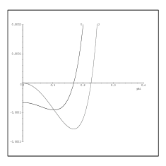
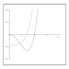
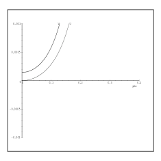
(a)                                   (b)                                   (c)

FIG. 2.: Comparison of classical potential $U$ and effective potential $V$ for (a) $r=-0.02$ and $a=-0.5$, (b) $r=-0.05$ and $a=-0.9$, and (c) $r=0.05$ and $a=0.5$.

FIG. 3.: Symmetry broken and unbroken regions in classical and $1$-loop effective theories.

REFERENCES

- [1] K. Halpern and K. Huang, Phys. Rev. Lett., 74, 3526 (1995).
- [2] K. Halpern and K. Huang, Phys. Rev. D, 53, 3252 (1996).
- [3] Kerson Huang, Quarks, Leptons, and Gauge Fields, World Scientific, 1992.
- [4] R. Jackiw, Phys. Rev. D9, 1686 (1974)
- [5] K.G. Wilson, Phys. Rev. Lett. 28, 248 (1972); K.G. Wilson and J. Kogut, Phys. Rep. C12, 75 (1974).
- [6] Vipul Periwal, Mod. Phys. Lett. A11, 2915, (1995).
- [7] J. Polchinski, Nucl. Phys. B231, 269 (1984).
- [8] M. Abramowitz and I.A. Stegun, Handbook of Mathematical Functions (National Bureau of Standards, Washington, 1964).
- [9] I.S. Gradshteyn and I.M. Ryzhik, Table of Integrals, Series, and Products, Fourth edition.
- [10] F.J. Wegner and A. Houghton, Phys. Rev., A8, 401 (1973).
(a) (b) (c)